TRANSPORTATION RESEARCH

RECORD No. 1413

Planning and Administration

Innovations in Travel Behavior Analysis,

Demand Forecasting, and Modeling Net-works

A peer-reviewed publication of the Transportation Research Board

TRANSPORTATION RESEARCH BOARD NATIONAL RESEARCH COUNCIL

NATIONAL ACADEMY PRESS· WASHINGTON, D.C. 1993

Transportation Research Record 1413 ISSN 0361-1981 ISBN 0-309-05560-1 Price: $31.00

Subscriber Category IA planning and administration

TRB Publications Staff Director of Reports and Editorial Services: Nancy A. Ackerman Associate Editor/Supervisor: Luanne Crayton Associate Editors: Naomi Kassabian, Alison G. Tobias Assistant Editors: Susan E. G. Brown, Norman Solomon Production Coordinator: Sharada Gilkey Office Manager: Phyllis D. Barber Senior Production Assistant: Betty L. Hawkins

Printed in the United States of America

Sponsorship of Transportation Research Record 1413

GROUP I-TRANSPORTATION SYSTEMS PLANNING AND ADMINISTRATION Chairman: Sally Hill Cooper, Virginia Department of

Transportation

Transportation Forecasting, Data, and Economics Section Chairman: Mary Lynn Tischer, Virginia Department of

Transportation

Committee on Passenger Travel Demand Forecasting Chairman: Eric Ivan Pas, Duke University Bernard Alpern, Moshe E. Ben-Akiva, Jeffrey M. Bruggeman, William A. Davidson, Christopher R. Fleet, David A. Hensher, Alan Joel Horowitz, Joel L. Horowitz, Ron Jensen-Fisher, Peter M. Jones, Frank S. Koppelman, David L. Kurth, T. Keith Lawton, David M. Levinsohn, Fred L. Mannering, Eric J. Miller, Michael R. Morris, Joseph N. Prashker, Charles L. Purvis, Martin G. Richards, Earl R. Ruiter, G. Scott Rutherford, Gala/ M. Said, Gordon W. Schultz, Peter R. Stopher, Antti Talvitie, A. Van Der Hoorn

Committee on Traveler Behavior and Values Chairman: Ryuichi Kitamura, University of California-Davis Elizabeth Deakin, Bernard Gerardin, Thomas F. Golob, David T. Hartgen, Joel L. Horowitz, Lidia P. Kostyniuk, Martin E. H. Lee-Gosselin, Hani S. Mahmassani, Patricia L. Mokhtarian, Frank Southworth, Peter R. Stopher, Janusz Supernak, Antti Talvitie, Mary Lynn Tischer, Carina Van Knippenberg, Martin Wachs, William Young

Committee on Transportation Supply Analysis Chairman: Hani S. Mahmassani, University of Texas at Austin David E. Boyce, Yupo Chan, Carlos F. Daganzo, Mark S. Daskin, Michel Gendreau, Theodore S. Glickman, Ali E. Haghani, Randolph W. Hall, Rudi Hamerslag, Bruce N. Janson, Haris N. Koutsopoulos, Chryssi Malandraki, Eric J. Miller, Anna Nagurney, Earl R. Ruiter, K. Nabil A. Safwat, Mark A. Turnquist

James A. Scott, Transportation Research Board staff

Sponsorship is indicated by a footnote at the end of each paper. The organizational units, officers, and members are as of December 31, 1992.

Transportation Research Record 1413

Contents

Foreword

Simulation Model of Activity Scheduling Behavior Dick Ettema, Aloys Borgers, and Harry Timmermans

Dynamic Interactive Simulator for Studying Commuter Behavior Under Real-Time Traffic Information Supply Strategies Peter Shen-Te Chen and Hani S. Mahmassani

Stated Preference Approach to Modeling the Adoption of Telecommuting Adriana Bernardino, Moshe Ben-Akiva, and Ilan Salomon

Employee Attitudes and Stated Preferences Toward Telecommuting: An Exploratory Analysis Hani S. Mahmassani, Jin-Ru Yen, Robert Herman, and Mark A. Sullivan

Choice Model of Employee Participation in Telecommuting Under a Cost-Neutral Scenario Mark A. Sullivan, Hani S. Mahmassani, and Jin-Ru Yen

Modeling Rail Access Mode and Station Choice Kai-Sheng Fan, Eric]. Miller, and Daniel Badoe

Central Area Mode Choice and Parking Demand Eric ]. Miller ·

Integrating Feedback into Transportation Planning Model: Structure and Application David Levinson and Ajay Kumar

v

1

12

22

31

42

49

60

70

Super-Regional, Very Long Range Transportation Modeling with a Geographic Information System David T. Hartgen, Yuanjun Li, and George Alexiou

Estimation of Travel Choice Models with Randomly Distributed Values of Time Moshe Ben-Akiva, Denis Bolduc, and Mark Bradley

Application and Interpretation of Nested Logit Models of Intercity Mode Choice Christopher V. Forinash and Frank S. Koppelman

Specifying, Estimating, and Validating a New Trip Generation Model: Case Study in Montgomery County, Maryland Ajay Kumar and David Levinson

Equilibrium Assignment Method for Pointwise Flow-Delay Relationships A. Regueros, ]. Prashker, and D. Mahalel

Properties of Vehicle Routes with Variable Shipment Sizes in Euclidean Plane Randolph W. Hall

An IP-Norm Origin-Destination Estimation Method That Minimizes Site-Specific Data Requirements Yupo Chan and M. Yunus Rahi

Integrated Structure of Long-Distance Travel Behavior Models in Sweden Staffan Algers

78

88

98

107

114

122

130

141

Foreword

The papers in this Record may be grouped into four topic areas: travel behavior models and simulation, modeling telecommunications attitudes and preferences, mode choice applica­tions, and transportation planning modeling and applications.

Papers in. the travel behavior models and simulation area address estimation of discrete travel choice models with no randomly distributed variables with time, a simulation model of activity scheduling behavior, and simulation for laboratory studies of the dynamics of commuter behavior under real-time information.

Papers in the telecommunications area are focused on a stated preference approach to . modify the adoption of telecommuting, employee attitudes and preferences toward tele­commuting, and a choice model of employee participation in telecommuting.

Papers in the mode choice area cover modeling rail access mode and station choice, central area mode choice and parking demand, and appreciation of nested logit models of intercity mode choice.

Papers in the transportation planning modeling area describe a new structure for trans­portation planning models; application of a geographic information system-based modeling system to a regional transportation problem; specification, estimation, and validation of a new trip generalization model; a new equilibrium assignment model; and a study of the geometric properties of vehicle routes that carry shipments of variable size.

v

TRANSPORTATION RESEARCH RECORD 1413

Simulation Model of Activity Scheduling Behavior

DICK ETTEMA, ALOYS BORGERS, AND HARRY TIMMERMANS

The simulation model of activity scheduling behavior presented is influenced by recent theories of activity scheduling and pro­duction system modeling. The basic assumption underlying the model is that activity scheduling is a sequential process in which consecutive steps lead to the final schedule. Every step in this respect is modeled as a choice of an action to perform on a preliminary schedule. The behavior of the model was tested using simulations in different hypothetical spatio-temporal settings. The simulations were conducted repeatedly, varying the values of the parameters of the model systematically. In general, the simula­tions resulted in realistic schedules. The proposed approach there­fore offers possibilities to model activity scheduling realistically. The next step, however, should be to develop calibration methods so that parameter values can be derived from observed behavior. Interactive simulations may be a promising technique in this respect.

Over the past few decades, travel has been increasingly re­garded as a derivative of activities, implying that knowledge about the way people choose activities to perform and sched­ule these in space and time is crucial for understanding and predicting travel behavior (J). As a result of changing roles and lifestyles of individuals, activity patterns and travel be­havior become increasingly more complex, making it difficult to forecast the impact of policy measures affecting travel be­havior. The goal of travel behavior research therefore has moved from predicting single travel decisions to understand­ing how many of the mutually related decisions that lead to activity patterns and their associated travel behavior are made. Consequently, activity scheduling behavior has become a topic of interest. Activity scheduling can be regarded as the plan­ning process preceding travel that determines what activities to perform and in which sequence the locations, the starting and ending hours of activities, and the route and travel modes are chosen.

Certain aspects of activity scheduling behavior have been addressed by such approaches as trip chaining models, activity choice models, time allocation models, and descriptive studies using activity diaries. [A discussion of these efforts is beyond the scope of this paper, refer to Kitamura (2) for a review.] To date, however, the only comprehensive model of activity scheduling is the STARCHILD model (3,4), which can be regarded as an extension of constraint-based approaches such as CARLA (J) and PESASP (5). Both CARLA and PESASP are based on Hagerstrand's space-time prism concept (6). ST AR CHILD uses a combinatorial algorithm to create all feasible patterns in a given situation and then selects the most

Department of Architecture and Urban Planning, Eindhoven Uni­versity of Technology, Postvak 20, P.O. Box 513, 5600 MB Eind­hoven, The Netherlands.

attractive pattern. The approach assumes optimal choice be­havior and the ability to select the best pattern out of a very large set.

This paper presents an alternate approach inspired by the theories of Root and Recker (7) and Garling et al. (8) and production system modeling. The model assumes a heuristic, suboptimal way of problem solving. In addition to activity schedule characteristics, the model also incorporates the cost of scheduling effort, implying that the expected utility of the schedule is weighted against the efforts needed to find a better schedule.

The remainder of this paper ·discusses the following:

• Theoretical considerations concerning activity schedul­ing. The two most comprehensive theories of activity sched­uling, the SCHEDULER framework (8) and the theory de­veloped by Root and Recker (7), are briefly described.

• A model based on the theoretical insights to activity scheduling. This model will also be compared with the existing scheduling model STARCHILD. ,

• Testing the activity scheduling model using simulations in different hypothetical spatio-temporal settings and the re­sults of these simulations.

• The results and possibilities of the modeling technique and some directions for future research are addressed.

THEORIES OF SCHEDULING BEHAVIOR

As activity pattern research has focused primarily on descrip­tive studies of revealed patterns, little documentation on the process underlying activity scheduling is available. The two most comprehensive frameworks to date have been developed by Root and Recker (7) and Garling et al. (8).

Root and Recker state that individuals will generate activity patterns that give them maximum utility, subject to con­straints such as opening hours of facilities and performance of the transportation system. That is, the utility gained from participation in activities is weighted against the disutility of travel needed for participation. Regarding the choice process preceding the formulation of an activity pattern, some re­marks are made. First, the disutility of the scheduling effort needed for complex trip chains may be greater than the utility of combining multiple sojourns in a single trip. Thus, the cost of scheduling will influence the outcome of the scheduling process. This is an important conclusion because it implies that activity scheduling cannot be regarded as an optimizing problem in the sense that travel is minimized or utility is maximized per se. Rather a satisficing process will take place

2

in which an acceptable schedule is created with acceptable effort.

Second, Root and Recker (7) distinguish a pretravel and a travel phase in the generation of activity patterns. In the pretravel phase, an activity program that maximizes the ex­pected utility is constructed based on expected activity du­rations and travel times. However, during execution, activities or trips may require more or less time than expected. De­pending on the pattern being "ahead" or "behind" schedule, the schedule may be adjusted by adding or removing activities or by changing the sequence or locations.

Finally, Root and Recker (7) point to the fact that the process of activity scheduling consists of several stages at which travel/activity decisions are taken. They assume that at each stage a utility is maximized, which consists of the utility of the travel decision itself and the expected utilities in later stages. The relation between the consecutive travel decisions can vary from completely independent, implying a suboptimal final result, to fully integrated, implying an optimal final re­sult. Thus, a stepwise decision process in which an optimi­zation occurs per step will lead to a more or less optimal solution.

The SCHEDULER theory [Garling et al. (8)] focuses spe­cifically on the scheduling process itself. The SCHEDULER framework assumes that some heuristic search is followed in the scheduling process. An individual is supposed to select a set of activities to be performed from the so-called long-term calendar (LTC). Also information is sought about when and where activities can be performed. On the basis of temporal constraints, the activities are first partially sequenced. The se­quence is then optimized using a nearest-neighbor heuristic (9).

Next, starting with the first activity, the schedule is mentally executed. This means that a more detailed schedule is formed in which mode choice, activity durations, travel times, and _waiting times are determined. In the stage of mental execu­tion, the first sequence formed may be altered if conflicts between activities (e.g., overlapping starting and finishing times) occur. Other possibilities are the replacement of an activity with an activity of lower priority or the adding of activities from the LTC when open time slots are present in the schedule. When the mental execution is finished, the first activity is carried out. It is important to note that the sched­uling process continues during the execution of the schedule. The schedule can then be revised if it cannot be executed as was initially expected.

It should be noted that the stepwise, suboptimal planning process of activity scheduling of the above theories is anal­ogous to problem-solving strategies that are studied in the field of cognitive science and artificial intelligence. It is as­sumed that individuals, when faced with complex problems, will use heuristic rules to find a solution path through the state space, mostly resulting in a satisfactory but not optimal solution (JO). Such heuristic search procedures are typically modeled by production systems, which are based on the way individuals store and process information. The application of production systems to activity scheduling has been suggested by Hayes-Roth and Hayes-Roth (11) and Golledge et al. (12). A problem with production systems, however, is that to date no calibration methods have been developed to match ob­served scheduling behavior and production systems. This is mostly due to the fact that the heuristics are defined in very

TRANSPORTATION RESEARCH RECORD 1413

specific IF ... THEN ... rules, making it difficult to gen­eralize the behavior of the model.

The model presented in this paper incorporates several ele­ments of the above frameworks: the stepwise construction and adaptation of the schedule, the suboptimal planning strat­egy, the use of heuristics avoiding the creation of all feasible patterns, and the incorporation of scheduling costs in the model. However, heuristics are defined in a more general way than is the case with production systems to make it easier to link the model to observed behavior.

SPECIFICATION OF MODEL

The task of the production system described in this section is to create a schedule for a 1-day period (7:00 a.m. to 12:00 p.m.). To complete this task, the following data are provided. An agenda containing activities to perform is assumed. The duration and the priorities of these activities are specified. Second, data are available on the opening times of facilities to perform activities, travel times between all pairs of loca­tions (so far no distinctions have been made among transport modes, and travel times are measured "as the crow flies"), and the attractiveness of the locations.

The scheduling process is assumed to be a sequential pro­cess consisting of a number of consecutive steps. In every step, the schedule, which is empty at the beginning of the process, can be adjusted by one of the following basic actions:

•Adding an activity from the agenda to the schedule. The activity can be inserted on every place in the sequence.

•Deleting an activity from the schedule. In this case, the deleted activity is placed on the agenda again.

• Substituting an activity from the schedule with an activity from the agenda. The new activity can be inserted on every place in the sequence.

•Stopping the scheduling process. In this case, the schedule created will be the final schedule.

Thus by repeatedly applying one of these basic actions, the schedule is constructed and adapted, until a satisfactory sched­ule is created. In the schedule, only the locations and the sequence of the activities are stored. It is believed that the exact starting and finishing times are determined by the actual duration of previous activities for temporally nonfixed activ­ities and are inherent to temporally fixed activities.

In every planning step, the production system creates all possibilities to perform the basic actions. For instance, in the case of substitution, all activities in the schedule can be re­placed by all activities on the agenda, which can be inserted on every place in the sequence. Of all possible variants, the action that gives the highest utility is performed. The utility of the stop action is zero by definition. This implies that the process is aborted if the utilities of all variants of the add, delete, and substitute actions are less than zero. The utilities of these actions are defined as follows:

9

+ ~j3 COUNTj + L -y1Y1 l=l

(1)

Ettema et al.

where

Vi = utility of action of type j (the action types will be denoted by subscripts add, del, and sub);

°'i = an alternative specific constant for action type j;

TIMESi = number of actions of specific type j that has been taken so far;

SINCEi = number of scheduling steps since last performance of action of type j;

COVNTi = number of scheduling steps applied so far in scheduling process, (this is an alternative specific variable for every action type);

COVNTi, TIMESi, and SINCEi = state-dependent variables of model;

13ik = a parameter indicating importance of state-dependent variable;

Y, = generic variables, namely, attri­butes of schedule resulting from ac­tion; and

'Yi = parameter indicating importance of attribute Y,.

Nine attributes of Y1 have been selected for the simulation experiment based on a literature search.

Attribute 1-The spatial configuration of the schedule. It is supposed that an individual tries to minimize distance within certain limits by spatially clustering activities. This clustering was observed in a "think aloud" protocol by Hayes-Roth and Hayes-Roth (11). The impact of the spatial configuration was also found by Garling et al. (9). The following measure of the degree of clustering (CONFIG) was developed:

(p 4= q) ifN?::.2 (2)

ifNs, 1

where

p, q = subscripts denoting locations visited in schedule, dpq = travel time between location p and location q, d = average travel time between all location pairs, and N = number of locations visited.

In the case of N;::::: 2, the first term is a measure of the deviation around the average mutual distance between all location pairs. The value will be 1 in the case of equal distances between all location pairs. In the case of outliers, this value and CONFIG will increase. The second part, being the average distance between all location pairs, implies that the value of CONFIG increases as the locations are more scattered about the area. Consequently, if the locations are situated very close to each other, d and therefore CONFIG will be almost zero. The value of CONFIG for situations with one location logically is determined at zero. Thus, the minimum value of CONFIG is zero in the case of optimal spatial concentration. In the case of more dispersed configurations or outliers, CONFIG increases.

3

Attribute 2-The time spent on activities. It is assumed that individuals try to maximize the amount of time spent on activities. The measure TIMEUSED is calculated as the sum of the durations of the scheduled activities, excluding travel time.

Attribute 3-The percentage of scheduled activities. As men­tioned before, individuals try to include as many activities as possible from the agenda in the schedule, especially those with a high priority; The measure· PERSCHED therefore is defined as the percentage of the activities on the agenda that are scheduled, in which the priority of every activity is used as a weighting factor:

_L Pr; PERSCHED = ~ · 100

_L Pr; iET

where

Pr; = priority of activity i, defined on a 0-10 scale, S = set of scheduled activities, and

(3)

T = set of activities, both scheduled and not, on agenda.

Attribute 4-The location of activities in the schedule in relation to the locations of activities not yet scheduled. This measure accounts for the propensity of individuals to incorporate fu­ture activities in .their scheduling decisions. It is assumed that one prefers to perform an activity on such a location that other activities can be performed in its vicinity. For instance, one might choose to do one's shopping at a particular mall because it offers the possibility to combine the trip with visits to the library, the post office, etc. A location is more attractive when other important activities can be included. This factor was also described in the experiment by Hayes-Roth and Hayes­Roth (11). Other empirical support comes from Kitamura (13), who found that the choice of a destination was influenced by the possibility to reach other locations afterward. The measure NEAROTH therefore can be defined as:

L L dr!/" Pri NEAROTH iES jER (4)

·where

di/" = travel time between location where i is performed and closest location where j can be performed,

Pr; = priority of activity i and is measured on a 0-10 scale, N5 = number of elements in S, NR = number of elements in R,

S = set of scheduled activities, and R = set of activities on agenda that have not yet been

scheduled.

Attribute 5-The attractiveness of the locations visited. It seems plausible that individuals try to optimize the utility of the schedule by visiting the locations with the highest utilities. For instance, Borgers and Timmermans (14,15) demonstrate

4

the influence of the floorspace of shops on the destination choice of pedestrians in shopping areas. To capture this effect, the measure UTILLOC (utility of locations) is given by:

LU; UTILLOC = ~

Ns

where

s = set of scheduled activities,

(5)

U; = utility of the location at which activity i is performed, and

N5 = number of activities scheduled.

Attribute 6-The total travel time implied by the schedule. It is recognized that individuals try to minimize the travel time and distance of their schedules within certain limits [see van der Hagen et al. (16)]. The measure TRA VTIME (travel time) accounting for this is simply the sum of the travel times between all consecutive pairs of locations in the schedule:

TRA VTIME = L D; (6)

where D; is the travel time for the ith trip.

Attribute 7-The latest possible finishing times of the scheduled activities. It is supposed that individuals prefer to schedule first those activities for which the least time is left. Lundberg (17) also uses this factor in his simulation model. To op­erationalize this measure, the latest possible finishing time (LASTEND) of the last activity in the schedule is taken.

Attribute 8-The length of open slots in the schedule. Recker et al. (3) mention the disutility derived from waiting times at locations out of home. It can therefore be assumed that people try to minimize waiting times implied by the schedule. To calculate a measure for this effect, all the wait­ing times implied by the sequence of activities, travel times, and opening hours of· facilities are summed. The measure W AITIIME is given by:

w AITIIME = 2: wi (7)

where W; is the duration of the ith waiting time.

Attribute 9-The chance of completing the schedule. In this stage of model development, it is checked whether the schedule can be executed given durations, travel times, and availability times. If a schedule can be performed, the measure CHANCE (chance of completing) is assigned the value 1, if it cannot be performed it is assigned the value 0. In a later phase, however, when durations and travel times are consid­ered to follow some statistical distribution, probabilities could be calculated more accurately.

The general behavior of the model will basically be_ deter­mined by the parameters O'. and ~ of Equation 1. Specifically, O'. and ~i2 will have positive values, and ~i1 and ~i3 will have

TRANSPORTATION RESEARCH RECORD 1413

negative values. This will lead to the execution of several ADD, DEL, and SUB actions before their utility decreases below zero due to the COUNT and TIMES variables. In that case, the STOP option is selected. By manipulating the exact parameter values, higher propensities to revise the schedule or to invest more effort in· the scheduling process itself can be simulated. The values Y1 determine which specific variant of an action type is selected. The values of the parameters 'Y in this respect indicate the importance of the attributes in every separate scheduling step. The parameters 'Y and the attribute values Y1 determine which variant of every action type is the most favorable. Finally, the action that has the highest utility implied by both the state-dependent and the other variables will be selected.

When compared with ST AR CHILD, the above model clearly adopts a different principle. According to the ST ARCHILD mechanism, an individual would be able to optimize his or her activity pattern by creating a large number of alternative patterns and select the most favorable. In reality, however, as mentioned by Root and Recker (7) and Garling et al. (8)

. individuals will use heuristic search procedures leading to suboptimal solutions.

The model presented here includes heuristic search pro­cedures by assuming a stepwise, sequential planning process. Analogous to the nearest neighbor heuristic, the best "fol­lowing step" is selected repeatedly, implying that suboptimal solutions will in principle be reached. In this process, the cost of scheduling is also accounted for. The heuristics used in the model are defined in a very general way, so that by manip­ulating the parameters of the model, the effect of the heu­ristics can be modified. In this regard, the model differs from production system models where heuristics are defined by very specific IF ... THEN ... rules. Therefore it will be easier to generalize the results of this model compared with production system models.

Finally, it is important to note that the mechanism of the model allows for the adjustment of the schedule during the travel phase. After completing an activity or a trip, the sched­ule for the rest of the planning period can be adjusted by the basic actions described earlier in this section. If and how the schedule is adjusted will depend on the utilities of possible adaptations and the utility of the existing schedule. The util­ities may be affected by congestion resulting in delayed travel times or unexpected durations of activities so that the chance of completing the schedule decreases. The impact of infor­mation on expected travel times in a congested area can be described in a similar way. Also, the priorities of activities may change during the course of day, affecting the utility of the schedule through the attributes PERSCHED and NEAROTH. In this way, activities with a short planning ho­rizon can be added to the schedule.

SIMULA TIO NS

The model described above was used to complete a simulation experiment that produced activity schedules in eight hypo­thetical spatio-temporal settings. Of these settings the follow­ing data were specified (see Table 1):

1. A travel time matrix containing travel times between every pair of locations.

TABLE 1 Description Scheduling Tasks

SITUATIONS 1,3 AND 4

activity

breakfast

work

going to grocery

preparing and having supper

sports

visiting friends

going to postoffice

going to bakery

going to library

deliver a parcel

utility loca­tion

10

5

1 5

10

10

2

1 5

5

8

2

earliest start time·

700

800

900 900

1800

1900

1900

900 900

900

900

900

latest end time

800

1800

1800 1800

2000

2300

2300

1750 1750

1800

2100

2100

priority (0-10 scale)

10

10

5

10

2

2

5

5

2

2

dura­tion· (0.01 hours)

25

800

25

150

150

100

15

10

25

5

SITUATIONS 5,7 AND 8

utility loca­tion

breakfast 10

bring children 5 to school

get children S from school

lunch 10

work 5

going to 5 grocery 1

preparing and 10 having supper

bring children to sports club

get children from sports club

go shopping 9

sports 3

visiting friends 8

earliest start time

700

825

1250

1300

800

900 900

1600

1900

2050

900

1900

1900

latest prio-end rity time (0-10

scale)

800 10

850 10

1300 10

1400 10

1300 10

1800 2 1800

1900 10

1905 10

2055 10

1800 2

2300 2

2300 2

dura­tion (0.01 hours)

100

5

s

75

300

15

ISO

s

s

40

100

100

SITUATION 2

utility loca­tion

10

5

1 5

10

10

2

1 5

5

8

2

ear­liest start time

700

800

900 900

1800

1900

1900

900 900

900

900

900

latest end time

800

1800

1900 1900

2000

2300

2300

1900 1900

1900

2100

2100

prio­rity (0-10 scale)

10

10

5

10

2

2

5

s

2

2

SITUATION 6

utility ear-loca- liest ti on start

10

5

5

10

s s 1

10

time

700

825

1225

1300

800

900 900

1600

latest prio-end rity time (0-10

scale)

800 10

875 10

1300 10

1400 10

1900 10

1900 2 1900

1900 10

1900 ~1905 10

9

3

8

2050 2055 10

900

1900

1900

1900 2

2300 2

2300 2

•for computational ease, an hour is determined to have 100 'minutes'

dura­tion

25

800

25

150

150

100

15

10

25

5

dura­tion

100

5

s

75

300

15

150

s

s

40

100

100

6

2. A list of activities to perform, with their priority and expected duration.

3. A specification of the utilities of all possible locations. 4. Information concerning where and when activities can

take place. For every activity, the locations and the opening hours of facilities are specified.

The eight situations relate to a hypothesized single working person and a hypothesized working parent, combining child care and work. The reason for this is that both groups are recognized to have problems executing their activity schedules under current spatio-temporal circumstances. In the first four situations, relating to a single working person, the same list of activities to perform is specified. The spatio-temporal set­tings however differ. Situations 1 and 2 relate to an urban setting, whereas situations 3 and 4 represent a suburban set­ting. In situation 2, shop hours are extended relative to sit­uation 1, and some facilities are located in the direct sur­roundings of the work location. Situations 3 and 4 are identical, except for the travel times, which are significantly shorter in situation 4. Because of the short travel time, either a bicycle or a car could be the transportation mode.

In situations 5 through 8, relating to a working parent com­bining child care and work, the same list of activities to per­form is specified. Situations 5 and 6 represent an urban set­ting, while situations 7 and 8 relate to a suburban/rural setting.

TRANSPORTATION RESEARCH RECORD 1413

Situations 5 and 6 differ in that situation 6 offers the more flexible work and shopping hours. In situation 7, most of the facilities are located in the city, but the residence is located in an adjacent village. In situation 8, all facilities are scattered about several municipalities.

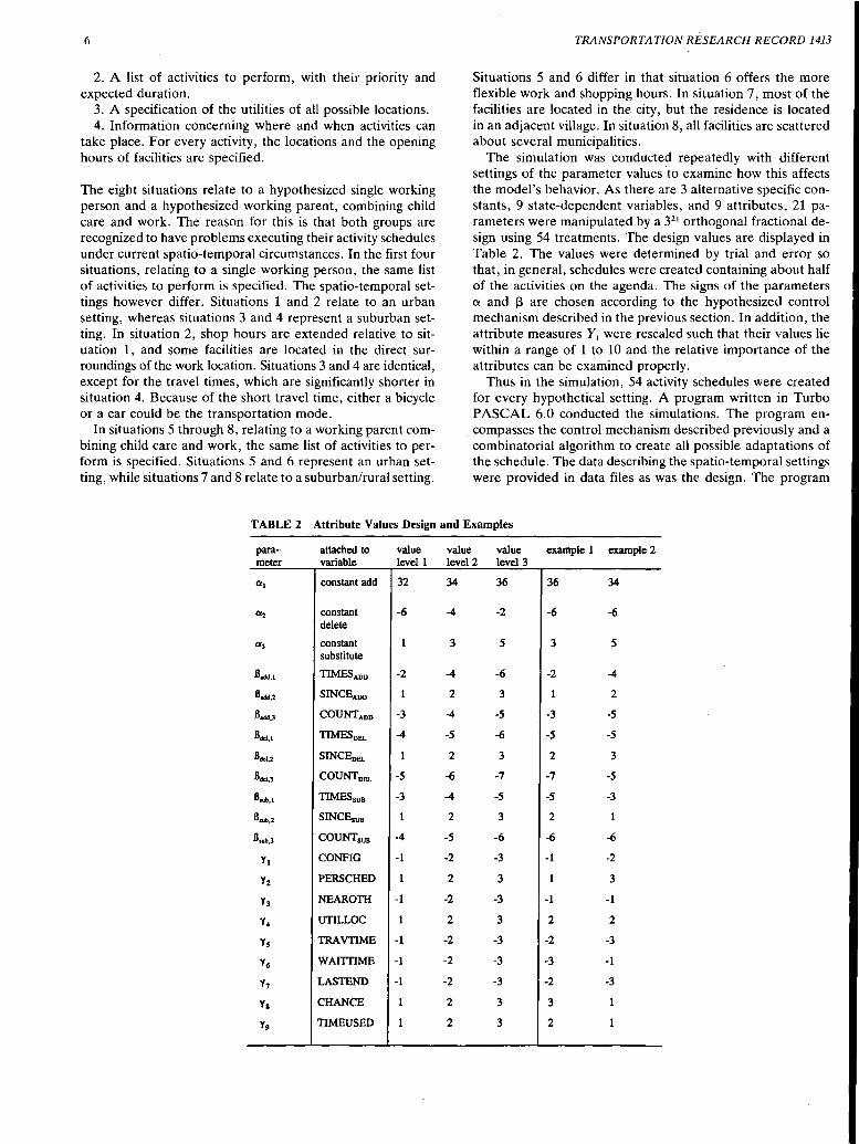
The simulation was conducted repeatedly with different settings of the parameter values to examine how this affects the model's behavior. As there are 3 alternative specific con­stants, 9 state-dependent variables, and 9 attributes, 21 pa­rameters were manipulated by a 321 orthogonal fractional de­sign using 54 treatments. The design values are displayed in Table 2. The values were determined by trial and error so that, in general, schedules were created containing about half of the activities on the agenda. The signs of the parameters a and '3 are chosen according to the hypothesized control mechanism described in the previous section. In addition, the attribute measures Y1 were rescaled such that their values lie within a range of 1 to 10 and the relative importance of the attributes can be examined properly.

Thus in the simulation, 54 activity schedules were created for every hypothetical setting. A program written in Turbo PASCAL 6.0 conducted the simulations. The program en­compasses the control mechanism described previously and a combinatorial algorithm to create all possible adaptations of the schedule. The data describing the spatio-temporal settings were provided in data files as was the design. The program

TABLE 2 Attribute Values Design and Examples

para- attached to value value value meter variable level 1 level 2 level 3

a 1 constant add 32 34 36

constant delete

a3 constant

.8..sd,1

.8add,3

.8dcl,l

substitute

TIMES ADD

COUNT DEL

TIMESsUB

COUNTsUB

CONFIG

Y2 PERSCHED

NEAROTH

Y4 UTILLOC

-6

-2

-3

-4

-5

-3

-4

-1

-1

Y, TRAVTIME -1

y6 WAITTIME -1

Y 7 LASTEND -1

Ya CHANCE

Y9 TIMEUSED

-4 -2

3 5

-4 -6

2 3

-4 -5

-5 -6

2 3

-6 -7

-4 -5

2 3

-5 -6

-2 -3

2 3

-2 -3

2 3

-2 -3

-2 -3

-2 -3

2 3

2 3

example 1 example 2

36 34

-6 -6

3 5

-2 -4

2

-3 -5

-5 -5

2 3

-7 -5

-5 -3

2

-6 -6

-1 -2

3

-1 -1

2 2

-2 -3

-3 -1

-2 -3

3

2

Ettema et al.

recorded the following data concerning the scheduling process and its outcome:

•The schedules created, that is, a list of activities that will be performed of which the sequence and location are determined;

•For every schedule, the attribute values (CONFIG, PERSCHED, NEAROTH, UTILLOC, TRAVTIME, WAITTIME, LASTEND, CHANCE, and TIMEUSED) of the schedule;

•For every schedule, the number of times every action type was applied (NRADD, NRDEL, and NRSUB); and

•For every schedule, the number of steps needed to create the schedule (NRSTEPS).

ANALYSIS

One of the main objectives of the simulation experiment was to find out if the proposed modeling approach generates re­alistic activity schedules. In this respect, it was examined what activities were included in the schedules and whether the char­acteristics of the schedules were affected logically by different hypothetical situations and different parameter sets.

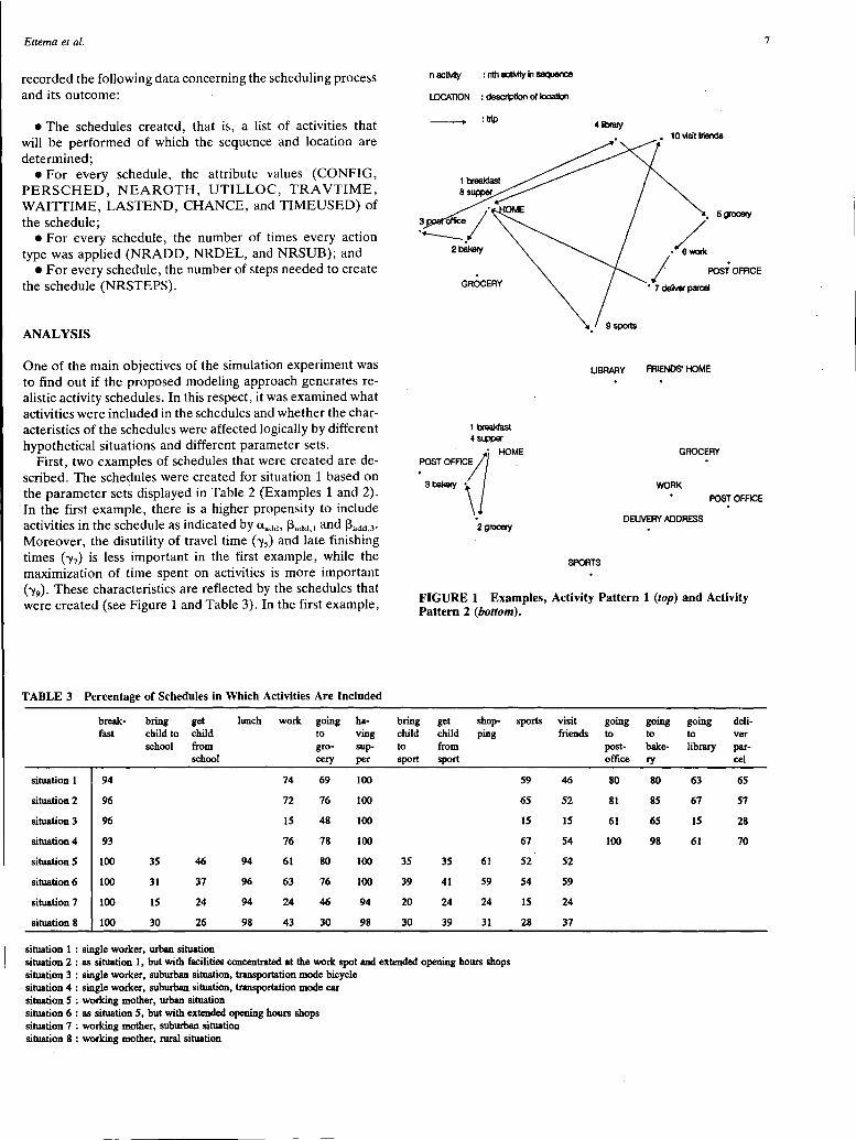
First, two examples of schedules that were created are de­scribed. The schedules were created for situation 1 based on the parameter sets displayed in Table 2 (Examples 1 and 2). In the first example, there is a higher propensity to include activities in the schedule as indicated by O'.actct• J3actct, 1 and J3actct,3 •

Moreover, the disutility of travel time ( -y5) and late finishing times ('Y7) is less important in the first example, ·while the maximization of time spent on activities is more important ('Y9). These characteristics are reflected by the schedules that were created (see Figure 1 and Table 3). In the first example,

TABLE 3 Percentage of Schedules in Which Activities Are Included

break- bring get lunch work going ha-fast child to child to ving

school from gro- sup-school cery per

situation 1 94 74 69 100

situation 2 96 72 76 100

situation 3 96 15 48 100

situation 4 93 76 78 100

situation 5 100 35 46 94 61 80 100

situation 6 100 31 37 96 63 76 100

situation 7 100 15 24 94 24 46 94

situation 8 100 30 26 98 43 30 98

situation 1 : single worker, urban situation

n activity : nth actMty In sequence

LOCATION : description of locatlon

:trip 4 lbrary

GROCERY

LIBRARY

• 10 visit friends

-~ Sgooety

I POSTOFACE

• 7 deiver paicel

FRIENDS' HOME

GROCERY

WORK POSTOFACE

DELIVERY ADDRESS 2 grocery

SPORTS

FIGURE 1 Examples, Activity Pattern 1 (top) and Activity Pattern 2 (bottom).

bring get shop- sports visit going going going deli-child child ping friends to to to ver to from post- bake- library par-sport sport office ry eel

59 46 80 80 63 65

65 52 81 85 67 51

15 15 61 65 15 28

67 54 100 98 61 70

35 35 61 52 52

39 41 59 54 59

20 24 24 15 24

30 39 31 28 37

situation 2 : as situation 1, but with facilities concentrated at the work spot and extended opening hours shops situation 3 : single worker, suburban situation, transportatio~ mode bicycle situation 4 : single worker, suburban situation, transportation mode car situation S : working mother, urban situation situation 6 : as situation 5, but with extended opening hours shops situation 7 : working mother, suburban situation situation 8 : working mother, rural situation

7

8

all activities are included. In the second example, only four activities are scheduled, of which only two are out of home. Consequently, more time is spent on travel (TRA VTIME) and activities (TIMEUSED) in the first example. The plan­ning horizon is also longer in this case (LAS TEND), and more effort is invested in the planning process (NRSTEPS). As more locations are visited, the degree of clustering is less in the first case (CONFIG). ·The waiting time out of home in both cases is zero. When looking at routing and sequencing, it can be concluded that distance is minimized and space is used efficiently. However, the sequence in which activities take place is somewhat unusual (shopping before work), as in this stage preferences for particular sequences are not yet incorporated in the model. It should be noted that the above examples represent two extreme situations based on extreme parameter sets, of which the second is especially unrealistic (e.g., work is excluded in the schedule). In most cases, how­ever, a considerable number of activities is included in an efficient schedule.

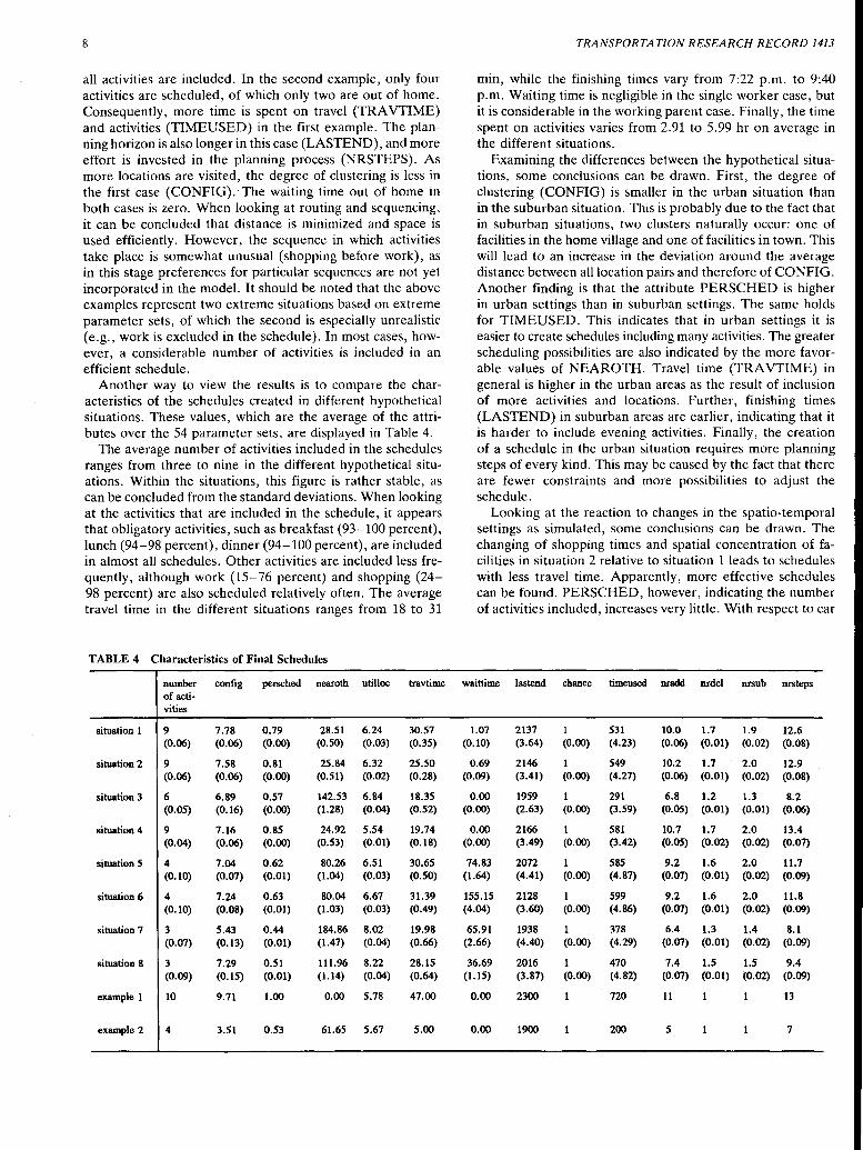
Another way to view the results is to compare the char­acteristics of the schedules created in different hypothetical situations. These values, which are the average of the attri­butes over the 54 parameter sets, are displayed in Table 4.

The average number of activities included in the schedules ranges from three to nine in the different hypothetical situ­ations. Within the situations, this figure is rather stable, as can be concluded from the standard deviations. When looking at the activities that are included in the schedule, it appears that obligatory activities, such as breakfast (93-100 percent), lunch (94-98 percent), dinner (94-100 percent), are included in almost all schedules. Other activities are included less fre­quently, although work (15-76 percent) and shopping (24-98 percent) are also scheduled relatively often. The average travel time in the different situations ranges from 18 to 31

TABLE 4 Characteristics of Final Schedules

number con fig persched nearoth utilloc travtime of acti-vi ties

situation 1 9 7.78 0.79 28.Sl 6.24 30.S7 (0.06) (0.06) (0.00) (O.SO) (0.03) (0.3S)

situation 2 9 7.SS 0.81 25.84 6.32 25.SO (0.06) (0.06) (0.00) (O.Sl) (0.02) (0.28)

situation 3 6 6.89 O.S7 142.S3 6.84 18.3S (O.OS) (0.16) (0.00) (1.28) (0.04) (O.S2)

situation 4 9 7.16 o.ss 24.92 S.S4 19.74 (0.04) (0.06) (0.00) (O.S3) (0.01) (0.18)

situation S 4 7.04 0.62 80.26 6.Sl 30.6S (0.10) (0.07) (0.01) (1.04) (0.03) (O.SO)

situation 6 4 7.24 0.63 80.04 6.67 31.39 (0.10) (0.08) (0.01) (1.03) (0.03) (0.49)

situation 7 3 S.43 0.44 184.86 8.02 19.98 (0.07) (0.13) (0.01) (1.47) (0.04) (0.66)

situation 8 3 7.29 O.Sl 111.96 8.22 28.lS (0.09) (0.lS) (0.01) (1.14) (0.04) (0.64)

example 1 10 9.71 1.00 0.00 S.78 47.00

example 2 4 3.Sl O.S3 61.6S S.61 S.00

TRANSPORTATION RESEARCH RECORD 1413

min, while the finishing times vary from 7:22 p.m. to 9:40 p.m. Waiting time is negligible in the single worker case, but it is considerable in the working parent case. Finally, the time spent on activities varies from 2.91 to 5.99 hr on average in the different situations.

Examining the differences between the hypothetical situa­tions, some conclusions can be drawn. First, the degree of clustering (CONFIG) is smaller in the urban situation than in the suburban situation. This is probably due to the fact that in suburban situations, two clusters naturally occur: one of facilities in the home village and one of facilities in town. This will lead to an increase in the deviation around the average distance between all location pairs and therefore of CONFIG. Another finding is that the attribute PERSCHED is higher in urban settings than in suburban settings. The same holds for TIMEUSED. This indicates that in urban settings it is easier to create schedules including many activities. The greater scheduling possibilities are also indicated by the more favor­able values of NEAROTH. Travel time (TRA VTIME) in general is higher in the urban areas as the result of inclusion of more activities and locations. Further, finishing times (LASTEND) in suburban areas are earlier, indicating that it is harder to include evening activities. Finally, the creation of a schedule in the urban situation requires more planning steps of every kind. This may be caused by the fact that there are fewer constraints and more possibilities to adjust the schedule.

Looking at the reaction to changes in the spatio-temporal settings as simulated, some conclusions can be drawn. The changing of shopping times and spatial concentration of fa­cilities in situation 2 relative to situation 1 leads to schedules with less travel time. Apparently, more effective schedules can be found. PERSCHED, however, indicating the number of activities included, increases very little. With respect to car

waittime las tend chance timeused nradd nrdel nrsub nrsteps

1.07 2137 1 S31 10.0 1.7 1.9 12.6 (0.10) (3.64) (0.00) (4.23) (0.06) (0.01) (0.02) (0.08)

0.69 2146 1 S49 10.2 1.7 2.0 12.9 (0.09) (3.41) (0.00) (4.27) (0.06) (0.01) (0.02) (0.08)

0.00 19S9 1 291 6.8 1.2 1.3 8.2 (0.00) (2.63) (0.00) (3.S9) (O.OS) (0.01) (0.01) (0.06)

0.00 2166 1 S81 10.7 1.7 2.0 13.4 (0.00) (3.49) (0.00) (3.42) (O.OS) (0.02) (0.02) (0.07)

74.83 2072 1 SSS 9.2 1.6 2.0 11.7 (1.64) (4.41) (0.00) (4.87) (0.07) (0.01) (0.02) (0.09)

lSS.lS 2128 1 S99 9.2 1.6 2.0 11.8 (4.04) (3.60) (0.00) (4.86) (0.07) (0.01) (0.02) (0.09)

6S.91 1938 1 378 6.4 1.3 1.4 8.1 (2.66) (4.40) (0.00) (4.29) (0.07) (0.01) (0.02) (0.09)

36.69 2016 1 470 7.4 1.S 1.S 9.4 (l.lS) (3.87) (0.00) (4.82) (0.07) (0.01) (0.02) (0.09)

0.00 2300 720 11 13

0.00 1900 200 s 7

Ettema et al.

availability (situation 4) relative to. bicycle availability (situ­ation 3), the simulations show an increase of PERSCHED and travel distance in case of car availability. In the case of the working parent in an urban situation, alleviating time constraints regarding work and shopping does not result in the inclusion of more activities and longer travel times. When the two suburban settings are compared, it can be concluded

TIMEUSED BOO.-------+-----~--------~

400

200

+

+ :j:

··----·------··--·······-··*-·····-----·-·-·--.... +

$ + ........ +. ...... .

o...._ __ ..__ __ ..._ __ ..._ __ ...__ __ ..._ __ ...___--J

0 0,5 1 1,5 2 2,5 3 3,5 gamma9 (TIMEUSED)

(a)

TAAVTIME 80

+ 60

+ +

40

:j:

20 +

+ + 0 -3.5 -3 -2,5 -2 -1,5 -1 -0.5 0

gamma1 (OONFIG) (c)

CON FIG 16,---------------------~

14r····-----------x-·--··---··-····--·--···-·····--·····-···--··----·-----~···--··-········-·-·-···--·-··-··-·········-···-·······················J +

12 --·-·-·----·-···-··--···-·-·····-····-·····-·······---·--··-·-·------ ···-··-··--··-·--·--··-··----···----······· :j: +

ior--·-------~----··--·-··---·--·-··----·--·--···------·-··--~~---·-·-·-····--·-------·····-----·-·-··········-··l

*

2 .. ······-···-····-··--··--··-$--·-··-··-·-···-··-····-····t····--·-·-·-···--·----$-···-·······----·-·--·····-··-···-·-····-···-·-·-·-·······

o----~-~-_._ _ _._ _ _.__---'*,____JL.___,L__..L.__~ 30 31 32 33 34 35 36 37 38 39 40

alpha ADD (e)

9

that PERSCHED in the city-oriented case (situation 7) is smaller and more time is needed for travel. The value of NEAROTH in the rural situation indicates that other activ­ities can be included more easily.

The results described above indicate that the model reacts logically to different spatio-temporal settings resulting from concentration of facilities, changes in opening hours, and

PERSCH ED 1,2 .-------------------------,

1 ····-·······-····-····-··t············-····-·-·······-··-·-·--···········---:i:····-··-·-·····-··-··----·---·-·---··-···:j:····-·--···-·······-.. ··-

+ a.a ·--·····-··---±-... ····-···--··-·-·--··---··-····-··--i--·-··-··-····-·-·· .. ·----·--·-·$· .. ·---··--··---···--·-····-

o.6 L~--=~~~:::::::::::=======+~=====t'F===:=.J 0,4 ... ········-···-·······l ........................................................... J ............ _ ........... ----··---·-·-···-····t··--········-··· ····--···--·······-·-······

+. t + 0.2

o..._ __ ...__ __ ..._, __ ..._ __ ...._ __ ...._ __ _.__ _ ____.

-3,5 -3 -2.5 -2 -1,5 -1 -0,5 0 gamma5 (TRAVTIME)

(b)

NRSTEPS 25r---------------------~

20 ········-··-·-·---··-··--···--·····-·--·-·-· + + ::j:

15 ....................... ······--···-·-···---··-···-·-······-

+ +

+

+ + . ··~ ····-··-···-·-·-·-···- ···-·-·--···--$····-

+

10L_--=··=·····-·=-····-=····-=·-·-=-·-·i ....... =.-= ... ::::::::::======t=--=-·······---.. -....... -........ -...... -...... ~ .... r ... ~--i

5 ........................................................... ,$ ...... .. ................... J ............................... _ ............. -....... -~ ............ . o..._ __ .__ __ .__ __ ...__ __ ....._ __ _._ __ _._ __ ~

0 0,5 1,5 2 2.5 3 3,5 gamma4 (UTILLOC)

(d)

NRADD 10,....-----------------------,

16 ·-···-·-··-·-----··---······ ............................ -···-·+·---·----·--········-······--·---·-

14~·--·-···-··--------··-·-·--·······-·-····-···· ·---·-·--r···-·--·-·-······-·--···--·············-~·--··-······················-··---······-····-···-··-·l

10

2 --···--·-·-··-·-··-----·- ······-··---·-·---···--····--····----·- ····-·····-·-···----·-·---·------·-···--····--··---

0 '----'----..__ __ ..._ __ ..._ __ ...._ __ _.__ _ ____,

-7 -6 -5 -4 -3 -2 -1 0

(f) beta ADD1 (TIMES)

FIGURE 2 Relations Between Parameters and Attributes of Schedules, Scattergrams and Regression Lines: (a) TIMEUSED, (b) PERSCHED, (c) TRA VTIME, (cl) NRSTEPS, (e) CONFIG, (f) NRADD.

10

changes in the transportation system. This is an important conclusion as the model should be used to evaluate policy measures as previously mentioned.

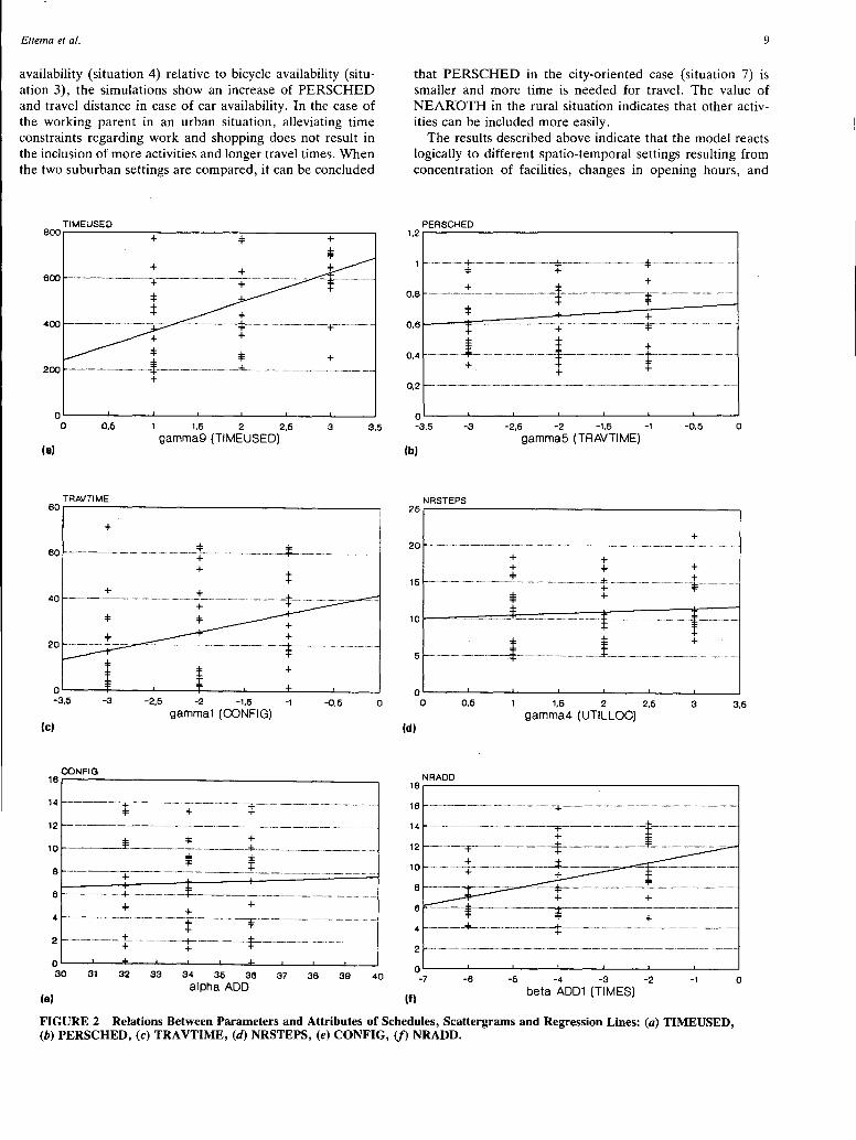
To gain iilsight in the mechanism of the model, the rela­tionship among the parameter values, indicating the weight of factors in each planning step and the characteristics of the schedules created at the end of the process is investigated. It appears that the influence of the 'Y parameters strongly influ­ences the Y attributes of the final schedules. For instance, a greater propensity to allocate time to activities during the scheduling process ( "!9) leads to more time allocated to activ­ities in the final schedule (TIMEUSED). This is illustrated in Figure 2a. (To facilitate interpretation, the scattergram and the regression line are displayed.) The parameters can also influence other attributes of the final schedule. For instance, when travel time is less important ("15), more activities are included in the schedule (PERSCHED, Figure 2b). When the spatial configuration is less emphasized ('Yi), travel times in­crease (Figure 2c). The 'Y parameters may also influence the scheduling process itself. For instance, a greater importance of the utility of locations ( 'Y4 ) requires more steps to reach an acceptable schedule and causes higher values of NRSTEPS (Figure 2d).

However, the importance of the state-dependent variables also influences the outcome of the scheduling. For instance, a higher value of O'.actct• indicating a higher propensity to include activities, results in more dispersed locations (CONFIG) in the final schedule (Figure 2e). Logically, the a and f3 param­eters will also determine the scheduling process itself. As can be seen from Figure 2f, for instance, less importance of the TIMESactct attribute (as indicated by f3actct, 1) leads to the exe­cution of more add-actions in the process.

The above examples indicate that the model reacts logically to changes in the parameter values. All relations among pa­rameters of the model and characteristics of the final schedules are summarized in Table 5 where each of these variables was

TABLE 5 Results Regression Analyses

parameter Y1 Y2 Y, Y4 Ys y, Y1 Y1

variable con per near util trav wait last chance fig sched oth loc time time end

d v con fig 2.19 1.64 0.94 0.65 0.69 1.14 1.49 e a

0.86 p r per 1.58 2.00 0.48 0.68 1.43 1.56

e i sched

n a nearoth -0.97 -0.97 -0.75 -0.49 -0.83 d b e l utilloc -0.41 -0.50 -0.57 -0.57 -0.33

n e travtime 1.99 1.98 1.12 1.16 1.54 1.96 t s

waittime 0.15 0.13 0.15 0.18

lastend 0.29 0.36 0.29

time 3.63 3.20 1.48 0.89 1.25 2.39 2.81 used

nradd 0.95 1.46 0.67 0.44 0.50 2.00 1.23

nrdel 0.25 0.16 0.28 0.24

nrsub 0.28 0.38 0.34

nrsteps 1.19 2.09 0.93 0.60 0.50 0.39 1.66 1.80

• only the coefficients significant at a = 0.05 are displayed

TRANSPORTATION RESEARCH RECORD 1413

used as the dependent variable in a regression analysis in which the parameter values a, f3, and 'Y served as explanatory variables. Generally, it can be concluded that the relationships among parameter values and characteristics of the schedule have the expected sign.

CONCLUSION AND DISCUSSION OF RESULTS

This paper presented a simulation model of activity scheduling to test the behavior of such a model responding to different circumstances. The results indicate that the simulation model reacts logically to different parameter settings and differences in spatio-temporal settings. The schedules created also seem reasonable in the sense that a considerable number of activ­ities are included in most schedules and that travel time is minimized to some extent. This implies an efficient use of time and space.

The above results give rise to the expectation that the pro­posed approach can realistically model activity scheduling be­havior. Of course, improvements, such as the incorporation of mode choice, the planning of time spent home, and con­straints in the sequence of activities (so that, for instance, shopping is not planned before work), remain to be made.

The next major step is to link the model to observed be­havior so as to derive parameter values. In this respect, in­teractive simulations may be a promising technique. In such experiments, subjects are asked to complete a task consisting of several steps. After each step, subjects are given infor­mation on the results of that step. In the case of activity scheduling, these scheduling steps can be recorded in a stan­dardized way by allowing the subjects to perform only the basic actions for the specification of the model. Because the explanatory variables can also be recorded, the relation be­tween the action chosen and the explanatory variables can be examined. In this respect, every planning step could princi-

aodd .Bodd,l y.,

.Bodd,3 .8c1o1,2 .8c1o1,3 a..., .8..,,,,2 .8..,,,,3

R2 time const times count since count const since count used (add) (add) (add) (del) (del) (sub) (sub) (sub)

1.83 0.25 0.75 0.68 0.98

2.79 0.34 1.30 1.35 -0.79 0.99

-1.41 0.17 -0.68 0.97

-0.47 -0.32 -0.25 0.99

3.21 0.17 1.46 1.60 -0.68 0.98

0.32 0.15 0.24 -0.09 0.06 0.90

0.76 0.19 1.00

5.28 0.59 1.84 1.72 -0.45 0.99

2.08 0.24 0.81 0.90 0.99

0.33 0.04 0.18 0.30 0.98

0.48 -0.19 -0.26 0.35 0.36 0.93

2.88 0.27 0.61 0.72 0.47 0.97

Ettema et al.

pally be modeled as a choice between several actions resulting in different preliminary solutions. The authors plan to per­form such an interactive experiment in early 1994. Further research therefore will have to focus on calibration methods for sequential choice models that can model the consecutive decisions in the scheduling process in their mutual coherence.

REFERENCES

1. Jones, P. M., M. C. Dix, M. I. Clarke, and I. G. Heggie. Under­standing Travel Behavior. Gower, Aldershot, England, 1983.

2. Kitamura, R. An Evaluation of Activity-based Analysis. Trans­portation, Vol. 15, No. 1, 1988, pp. 9-24.

3. Recker, W.W., M. G. McNally, and G. S. Root. A Model of Complex Travel Behavior: Part 1: Theoretical Development. Transportation Research, Vol. 20A, No. 4, July 1986, pp. 307-318.

4. Recker, W.W., M. G. McNally, and G. S. Root. A Model of Complex Travel Behavior: Part 2: An Operational Model. Trans­portation Research, Vol. 20A, No. 4, July 1986, pp. 319-330.

5. Lenntorp, B. A Time-Geographic Simulation Model of Individ­ual Activity Programmes. In Human Activity and Time Geog­raphy, (Vol. 2) (T. Carlstein, D. Parkes, and N. Thrift, eds.), Edward Arnold, London, 1978, pp. 162-180.

6. Hagerstrand, T. What about People in Regional Science? Papers of the Regional Science Association, Vol. 24, 1970, pp. 7-21.

7. Root, G. S., and W. W. Recker. Toward a Dynamic Model of Individual Activity Pattern Formulation. In Recent Advances in Travel Demand Analysis (S. Carpenter and P. Jones, eds.), Gower, Aldershot, 1983, pp. 371-382.

8. Garling, T., K. Brannas, J. Garvill, R. G. Golledge, S. Gopal, E. Holm, and E. Lindberg. Household Activity Scheduling. Pre­sented at 5th World Conference on Transport Research, Yo­kohama, Japan, 1989.

11

9. Garling, T., J. Saisa, A. Book, and E. Lindberg. The Spati­otemporal Sequencing of Everyday Activities in the Large-Scale Environment. 'Journal of Environmental Psychology, Vol. 6, No. 4, Dec. 1986, pp. 261-280.

10. Simon, H. A. Invariants of Human Behavior. Annual Review of Psychology, Vol. 41, 1990, pp. 1-19.

11. Hayes-Roth, B., and F. Hayes-Roth. A Cognitive Model of Plan­ning. Cognitive Science, Vol. 3, No. 4, Oct.-Dec. 1979, pp. 275-310.

12. Golledge, R. G., M. Kwan, and T. Garling. Computational Pro­cess Modelling of Travel Decisions: Empirical Tests. Prepared for the North American Regional Science Meetings, New Or­leans, Nov. 1991.

13. Kitamura, R. Incorporating Trip Chaining into Analysis of Des­tination Choice. Transportation Research, Vol. 18B, No. 1, 1983, pp. 67-81.

14. Borgers, A., and H. Timmermans. City Centre Entry Points, Store Location Patterns and Pedestrian Route Choice Behavior: A Microlevel Simulation Model. Socio-Economic Planning Sci­ences, Vol. 20, No. 1, 1986, pp. 25-31.

15. Borgers, A., and H. Timmermans. A Model of Pedestrian Route Choice and Demand for Retail Facilities within Inner-City Shop­ping Areas. Geographical Analysis, Vol. 18, No. 2, April 1986, pp. 115-128.

16. Van der Hagen, X., A. Borgers, and H. Timmermans. Spati­otemporal Sequencing Processes of Pedestrians in Urban Retail Environments. Papers in Regional Science, Vol. 70, No. 1, Jan. 1991, pp. 37-52. .

17. Lundberg, C. G. On the Structuration of Multiactivity Task­Environments. Environment and Planning A, Vol. 20, No. 12, Dec. 1988, pp. 1,603-1,621.

Publication of this paper sponsored by Committee on Traveler Be­havior and Values.

12 TRANSPORTATION RESEARCH RECORD 1413

Dynamic Interactive Simulator for Studying Commuter Behavior Under Real-Time Traffic Information Supply Strategies ·

PETER SHEN-TE CHEN AND HANI s. MAHMASSANI

A new simulator for laboratory studies of the dynamics of com­muter behavior under real-time traffic information (advanced traveler information systems) strategies is described, and a set of laboratory experiments that used this simulator is discussed. The purpose of the experiments was to examine the behavioral pro­cesses underlying commuter decisions on route diversions en route and day-to-day departure time and route choices as influenced by the provision of real-time traffic information. Both the real­time and day-to-day dynamic properties of traffic networks under alternative information strategies-particularly issues of conver­gence to an equilibrium, stability, and benefits following shifts in com~uter trip timing decisions-will also be investigated in the expenments.

Various efforts have been initiated worldwide to develop in­telligent vehicle highway systems (IVHSs). Major demon­stration projects and research programs can be found in the United States, Europe, and Japan (1-4). There are three general clusters of IVHS technologies with application to com­muter mobility: advanced traffic management systems (ATMS), advanced traveler information systems (A TIS), and advanced vehicle control systems (AVCS) (5). Essentially, IVHS uses advanced information processing and communications tech­nologies to manage traffic, advise drivers, and, eventually, control the flow of vehicles to improve efficiency and safety.

A TIS is especially targeted to assist drivers in trip planning and decision making on destination selection, departure time and route choices, congestion avoidance, and navigation to improve the convenience and efficiency of travel (6, 7). Var­ious A TIS classes have been defined from Class 0 static, open­loop systems, to Class 4 dynamic, closed-loop systems, ena­bling two-way communication between the vehicle and the traffic control center (8). Because of limited real-world im­plementation of A TIS technologies, it has been impractical for researchers to evaluate how real-time information avail­ability influences driver behavior. The purpose of this paper is to introduce a dynamic multi-driver interactive simulator as ai tool to assess travel behavior in response to ATIS infor­mation supply features. Special attention is given to the spa­tial/temporal context of the potential responses.

Several methodological approaches have been proposed to assess the effectiveness of various possible forms of A TIS to reduce recurrent and nonrecurrent traffic congestion and ex-

Department of Civil Engineering, University of Texas at Austin Austin, Tex. 78712. '

amine the interactions among key parameters, such as nature and amount of information displayed, market penetration, and congestion severity (9-13). Furthermore, various human factors studies have been conducted concerning the atten­tional demand requirements of in-vehicle navigation devices and their effects on the safety of driver performance, using either a driving simulator or specially adapted vehicles in real urban environments (14-16). Mail-back surveys and tele­phone interviews on drivers' willingness to divert en route in response to real-time traffic information and their preferences toward the different features of these systems have also been conducted (17-20).

Three computer-based interactive simulators have been de­veloped to study commuter behavior through laboratory ex­periments as an alternative and precursor to real-world ap­plications. Interactive Guidance on Routes (IGOR) was developed by Bonsall and Parry for investigating factors af­fecting drivers' compliance with route guidance advice, such as quality of advice and familiarity with the network (21). Allen et al. used an interactive simulator to study the impacts of different information systems on drivers' route diversion and alternative route selection (22). Freeway and Arterial Street Traffic Conflict Arousal and Resolution Simulator (FASTCARS), developed by Adler et al., was used to predict en route driver behavior in response to real-time traffic con­dition information based on conflict assessment and resolution theories (23). All these simulators are deterministic, with all traffic conditions and consequences of driver actions prede­termined, and no consideration of network-wide traffic char­acteristics. These simulators can interact with only one subject at any given time, ignoring interactions among drivers in the same traffic system. Bonsall and Parry's simulator provides different preset levels of information quality to the experi­mental subject in a preset sequence. In addition, the effect of the drivers' responses to the information on the traffic system is not considered. The simulators of both Allen et al. and Adler et al. assume the information supplied to be correct and static, which does not represent actual real-time A TIS environments.

Driver behavior and responses to real-time traffic infor­mation systems are the result of a complex process involving human judgment, learning, and decision making in a dynamic environment. Uncertainty in this dynamic environment orig­inates from the fact that (a) the consequences of an individual

Chen and Mahmassani

driver's decision depends on the decisions of other drivers in the network and (b) the interactions that determine these outcomes take place in the traffic system and are highly non­linear. In particular, a "recommended" path predicated on current link trip times may be less than optimal as congestion in the system evolves. Hence, the accuracy of the information provided to participating drivers and the resulting reliability of this information as a basis for route choice decisions are governed by the dynamic nature of the driver-decision envi­ronment and the presence of collective effects in the network as a result of the interactions of a large number of individual decisions (24,25). Consequently, driver decisions on the ac­quisition of the information system and compliance with its instructions are influenced by the users' perceptions of the reliability and usefulness of the system. These perceptions are formed mostly by learning through one's own experience with the system, as well as reports by friends, colleagues, and popular media. This is a long-term process that depends on the type and nature of the information provided, in addition to the individual characteristics and preferences of the driver.

The ideal way to study this long-term process is by observing actual driver decisions in real-world systems. However, as noted earlier, in the absence of sufficient deployment of the technologies of interest, it is practically difficult to obtain real­world data on the actual behavior of drivers under different real-time information strategies, on a daily basis, together with the various performance measures affecting these re­sponses. A set of controlled "laboratory-like" interactive ex­periments involving real commuters in a simulated traffic sys­tem is proposed in this paper, following Mahmassani and Herman's work on interactive experiments for the study of tripmaker behavior dynamics (26). Such experiments could play an important transitional role in gaining fundamental insights into behavioral phenomena that will play a key role in determining the effectiveness of A TIS and A TMS strategies.

This paper describes a new simulator, developed at the University of Texas at Austin, that offers the capability for real-time interaction with and among multiple driver partic­ipants in a traffic network under A TIS strategies. The sim­ulator allows several tripmakers to "drive" through the net­work, interacting with other drivers and contributing to system evolution. It considers both system performance as influenced by driver response to real-time traffic information and driver behavior as influenced by real-time traffic information based on system performance. The simulators reviewed earlier are primarily computer-based devices that display predetermined stimuli and elicit and collect the participants' responses. The simulator described here actually simulates traffic. Its "en­gine" is a traffic flow. simulator and A TIS information gen­erator that displays information consistent with the processes actually taking place in the (simulated) traffic system under the particular information supply strategy of interest. The decisions made by the driver participants are fed directly to the simulator and as such influence the traffic system itself and the subsequent stream of information stimuli provided to the participants.

In addition to studying users' responses to A TIS informa­tion for a particular commute on a given day, the simulator allows the researcher to investigate the day-to-day evolution of individual decisions under such information strategies. This longer-term dimension is missing from most available studies

13

of the effectiveness of real-time information systems. Our experiments consider system evolution and possible equili­bration by including the participants and the performance simulator in a loop whereby tripmakers may revise their de­cisions from one iteration day to the next. These experiments are intended to investigate both the real-time and day-to-day dynamic properties of traffic networks under alternative in­formation strategies, particularly issues of convergence to an equilibrium, stability, and benefits following shifts in user trip timing decisions.

The context for this paper is that of morning peak-period commuters in congested traffic corridors. The intended in­teractive experiments can be divided into three categories: (a) pre-trip and en route path selection only, (b) pre-trip departure time and path choice and en route path selection, and (c) pre-trip departure time and path choice, real-time departure time adjustments and en route path selection. In each category, each subject is asked to "drive" a vehicle to the central business district (CBD) through a corridor net­work. Each subject (or user) is provided with real-time traffic information before each trip. On the basis of this information, the user independently supplies his or her departure time and path decisions. These decisions are in turn fed into a traffic simulation and path assignment model (11,12). Each subject's vehicle is then moved along the selected path according to the prevailing traffic condition on the link that the vehicle is on. At each junction where the user has the opportunity to switch to an alternative route, he or she is again provided with real-time traffic information and asked to decide whether to stay on the current path or switch to an alternative route. Feedback is supplied to the subject at the end of the trip on the consequences of his or her decisions and new decisions are sought accordingly for the next day's trip. This process is repeated until system convergence is achieved or a predeter­mined number of iterations is exceeded.

SIMULATOR DESCRIPTION

System Architecture

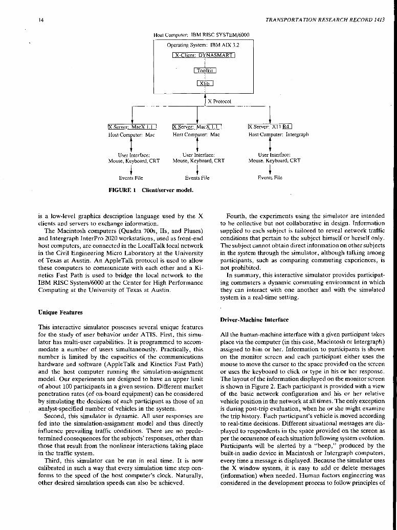
The simulator developed to perform the interactive experi­ments is an application of the client/server modeling concept used extensively in X Window System applications (27) (see Figure 1). The simulation-assignment model (as an X client) used is an extension of the corridor model developed by Mah­massani and J ayakrishnan (9) and modified by Mahmassani and Chen (10) to include pre-trip path selection in addition to en route switching decisions. The code for this model was written in FORTRAN and is run on an IBM RISC System/ 6000 (as a host computer). An additional program (as another X client) was written using X library functions (X Window System, version 11, release 3) to control the layout of windows displayed on the screens of a set of Macintosh and Intergraph computers (used by subjects, one computer per subject) on which either MacX 1.1 (for Macintoshes) or Xll R4 (for Intergraphs) is being run. Written in C, this program is linked to the simulation-assignment model using a number of C li­brary interface routines available under IBM AIX, version 3.2, an implementation of the AT&T System V-based version of the UNIX ·operating system. X Window System protocol

14 TRANSPORTATION RESEARCH RECORD 1413

Host Computer: IBM RISC SYSTEM/6000

Operating System: IBM AIX 3.2

I X-Client: DYNASMART I

Host comrt•c Mac

User Interface:

,I /

~lkiLJ i

rxi[D X Protocol

Server: MacX 1.1

Host comr•" Mac

. User Interface:

Host CoTutec Intergraph

User Interface: Mouse, Keyboard, CRT Mouse, Keyboard, CRT Mouse, Keyboard, CRT

+ + Events File Events File

FIGURE 1 Client/server model.

is a low-level graphics description language used by the X clients and servers to exchange information.

The Macintosh computers (Quadra 700s, Us, and Pluses) and Intergraph InterPro 2020 workstations, used as front-end host computers, are connected in the LocalTalk local network in the Civil Engineering Micro Laboratory at the University of Texas at Austin. An AppleTalk protocol is used to allow these computers to communicate with each other and a Ki­netics Fast Path is used to bridge the local network to the IBM RISC System/6000 at the Center for High Performance Computing at the University of Texas at Austin.

Unique Features

This interactive simulator possesses several unique features for the study of user behavior under A TIS. First, this simu­lator has multi-user capabilities. It is programmed to accom­modate a number of users simultaneously. Practically, this number is limited by the capacities of the communications hardware and software (AppleTalk and Kinetics Fast Path) and the host computer running the simulation-assignment model. Our experiments are designed to have an upper limit of about 100 participants in a given session. Different market penetration rates (of on-board equipment) can be considered by simulating the decisions of each participant as those of an analyst-specified number of vehicles in the system.

Second, this simulator is dynamic. All user responses are fed into the simulation-assignment model and thus directly influence prevailing traffic conditions. There are no prede­termined consequences for the subjects' responses, other than those that result from the nonlinear interactions taking place in the traffic system.

Third, this simulator can be run in real time. It is now calibrated in such a way that every simulation time step con­forms to the speed of the host computer's clock. Naturally, other desired simulation speeds can also be achieved.

+ Events File

Fourth, the experiments using the simulator are intended to be collective but not collaborative in design. Information supplied to each subject is tailored to reveal network traffic conditions that pertain to the subject himself or herself only. The subject cannot obtain direct information on other subjects in the system through the simulator, although talking among participants, such as comparing commuting experiences, is not prohibited.

In summary, this interactive simulator provides participat­ing commuters a dynamic commuting environment in which they can interact with one another and with the simulated system in a real-time setting.

Driver-Machine Interface

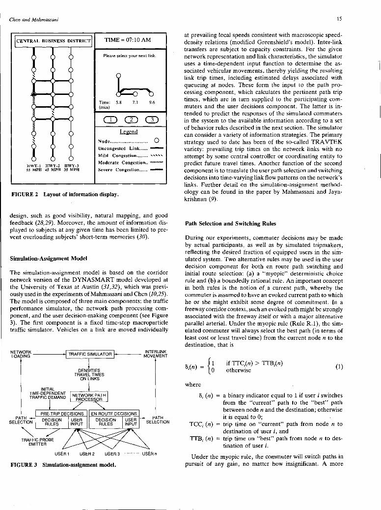
All the human-machine interface with a given participant takes place via the computer (in this case, Macintosh or Intergraph) assigned to him or her. Information to participants is shown on the monitor screen and each participant either uses the mouse to move the cursor to the space provided on the screen or uses the keyboard to click or type in his or her response. The layout of the information displayed on the monitor screen is shown in Figure 2. Each participant is provided with a view of the basic network configuration and his or her relative vehicle position in the network at all times. The only exception is during post-trip evaluation, when he or she might examine the trip history. Each participant's vehicle is moved according to real-time decisions. Different situational messages are dis­played to respondents in the space provided on the screen as per the occurrence of each situation following system evolution. Participants will be alerted by a "beep,'' produced by the built-in audio device in Macintosh or Intergraph computers, every time a message is displayed. Because the simulator uses the X window system, it is easy to add or delete messages (information) when needed. Human factors engineering was considered in the development process to follow principles of

Chen and Mahmassani

CENTRAL BUSINESS DISTRICT

HWY·l HWY-2 HWY-3 55 MPH 45 MPH 35 MPH

TIME= 07:10 AM

Please select your next link.

Time: 5.8 (min)

7.1 9.6

CD CD CD Legend

Node....................... 0 Uncongested Link ...... -

Mild Congestion ........................ ....

Moderate Congestion .. '''''''''"'

Severe Congestion ...... -

FIGURE 2 Layout of information display.

design, such as good visibility, natural mapping, and good feedback (28,29). Moreover, the amount of information dis­played to subjects at any given time has been limited to pre­vent overloading subjects' short-term memories (30).

Simulation-Assignment Model

The simulation-assignment model is based on the corridor network version of the DYNASMART model developed at the University of Texas at Austin (31,32), which was previ­ously used in the experiments ofMahmassani and Chen (10,25). The model is composed of three main components: the traffic performance simulator, the network path processing com­ponent, and the user decision-making component (see Figure 3). The first component is a fixed time-step macroparticle traffic simulator. Vehicles on a link are moved individually

~~~~~K -----·I TRAFFIC SIMULATOR' i... ·---- ~tgJER~~NNKT

INITIAL TIME-DEPENDENT TRAFFIC DEMAND

PATH SELECTION

USER 1

l DENSITIES,

TRAVEL TIMES ON LINKS

USER2

PATH SELECTION

USER 3 ............. USER fl

FIGURE 3 Simulation-assignment model.

15

at prevailing local speeds consistent with macroscopic speed­density relations (modified Greenshield's model). Inter-link transfers are subject to capacity constraints. For the given network representation and link characteristics, the simulator uses a time-dependent input function to determine the as­sociated vehicular movements, thereby yielding the resulting link trip times, including estimated delays associated with queueing at nodes. These form the input to the path pro­cessing component, which calculates the pertinent path trip times, which are in turn supplied to the participating com­muters and the user decisions component. The latter is in­tended to predict the responses of the simulated commuters in the system to the available information according to a set of behavior rules described in the next section. The simulator can consider a variety of information strategies. The primary strategy used to date has been of the so-called TRA VTEK variety: prevailing trip times on the network links with no attempt by some central controller or coordinating entity to predict future travel times. Another function of the seconfl component is to translate the user path selection and switching decisions into time-varying link flow patterns on the network's links. Further detail on the simulation-assignment method­ology can be found in the paper by Mahmassani and Jaya­krishnan (9).

Path Selection and Switching Rules

During our experiments, commuter decisions may be made by actual participants, as well as by simulated tripmakers, reflecting the desired fraction of equipped users in the sim­ulated system. Two alternative rules may be used in the user decision component for both en route path switching and initial route selection: (a) a "myopic" deterministic choice rule and (b) a boundedly rational rule. An important concept in both rules is the notion of a current path, whereby the commuter is assumed to have an evoked current path to which he or she might exhibit some degree of commitment. In a freeway corridor context, such an evoked path might be strongly associated with the freeway itself or with a major alternative parallel arterial. Under the myopic rule (Rule R.1), the sim­ulated commuter will always select the best path (in terms of least cost or least travel time) from the current node n to the destination, that is

8,{n) ~ { ~ where

if TTC;(n) > TTB;(n) otherwise

(1)

8; (n) a binary indicator equal to 1 if user i switches from the "current" path to the "best" path between node n and the destination; otherwise it is equal to O;

TCC; (n) = trip time on "current" path from node n to destination of user i, and

TTB; (n) = trip time on "best" path from node n to des­tination of user i.

Under the myopic rule, the commuter will switch paths in pursuit of any gain, no matter how insignificant. A more

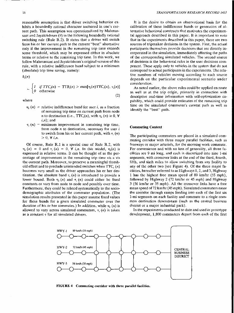
16

reasonable assumption is that driver switching behavior ex­hibits a boundedly rational character anchored in one's cur­rent path. This assumption was operationalized by Mahmas­sani and Jayakrishnan (9) in the following boundedly rational switching rule (Rule R.2). It states that a driver will switch from his or her current path to the current "best" alternative only if the improvement in the remaining trip time exceeds some threshold, which may be expressed either in absolute terms or relative to the remaining trip time. In this work, we follow Mahmassani and Jayakrishnan's original version of this rule, with a relative indifference band subject to a minimum (absolute) trip time saving, namely:

Bi(n)

where

'Yli (n)

T; (n)

if TTCJn) otherwise

TTB;(n) > max['Yl;(n)TTC;(n), T;(n)]

(2)

relative indifference band for user i, as a fraction of remaining trip time on current path from node n to destination (i.e., TTC;(n), with Tl; (n) 2: 0, \:/ i,n); and minimum improvement in remaining trip time, from node n to destination, necessary for user i to switch from his or her current path, with T; (n) > 0, \:/ i,n.

Of course, Rule R.1 is a special case of Rule R.2, with 'Yli (n) = 0 and Ti (n) = 0, \:/ i,n. In this model, 'Yl;(n) is expressed in relative terms. It can be thought of as the per­centage of improvement in the remaining trip time vis a vis the current path. Moreover, to preserve a meaningful thresh­old effect and to preclude unintended switches when TIC; (n) becomes very small as the driver approaches his or her des­tination, the absolute band Ti (n) is introduced to provide a lower bound. Both Tl; (n) and T; (n) could either be fixed constants or vary from node to node and possibly over time. Furthermore, they could be related systematically to the socio­demographic attributes of the commuter population. (The simulation results presented in this paper assume fixed values for these bands for a given simulated commuter over the duration of his or her commutes.) In addition, while Tl; (n) is allowed to vary across simulated commuters, T; (n) is taken as a constant T for all simulated drivers.

HWY -1 89 km/h (55 mph)

TRANSPORTATION RESEARCH RECORD 1413

It is the desire to obtain an observational basis for the calibration of these indifference bands or generation of al­ternative behavioral constructs that motivates the experimen­tal approach described in this paper. It is important to note that in the experiments described in this paper, there are two sources of tripmaker decisions in the system. First, the actual participants themselves provide decisions that are directly in­corporated in the simulation, immediately affecting the paths of the corresponding simulated vehicles. The second source of decisions is the behavioral rules in the user decisions com­ponent. These apply only to vehicles in the system that do not correspond to actual participants in the experiments. The rela­tive numbers of vehicles moving according to each source depends on the particular experimental scenario under consideration.

As noted earlier, the above rules could be applied en route as well as at the trip origin, primarily in connection with descriptive real-time information with self-optimization ca­pability, which could provide estimates of the remaining trip time on the simulated commuter's current path as well as identify the "best" path.

Commuting Context

The participating commuters are placed in a simulated com­muting corridor with three major parallel facilities, such as freeways or major arterials, for the morning work commute. For convenience and with no loss of generality, all .three fa­cilities are 9 mi long, and each is discretized into nine 1-mi segments, with crossover links at the end of the third, fourth, fifth, and sixth miles to allow switching from any facility to any of the other two (see Figure 4). Of the three major fa­cilities, hereafter referred to as Highways 1, 2, and 3, Highway 1 has the highest free mean speed of 89 km/hr (55 mph), followed by Highway 2 (72 km/hr or 45 mph) and Highway 3 (56 km/hr or 35 mph). All the crossover links have a free mean speed of 72 km/hr (45 mph). Simulated commuters enter the corridor through ramps feedfog into each of the first six 1-mi segments on each facility and commute to a ~ingle com­mon destination downstream (such as the central business district or a major industrial park).

In the experiments conducted to date and used in prototype development, 1,800 commuters depart from each of the first

CENTRAL BUSINESS DISTRICT

FIGURE 4 Commuting corridor with three parallel facilities.

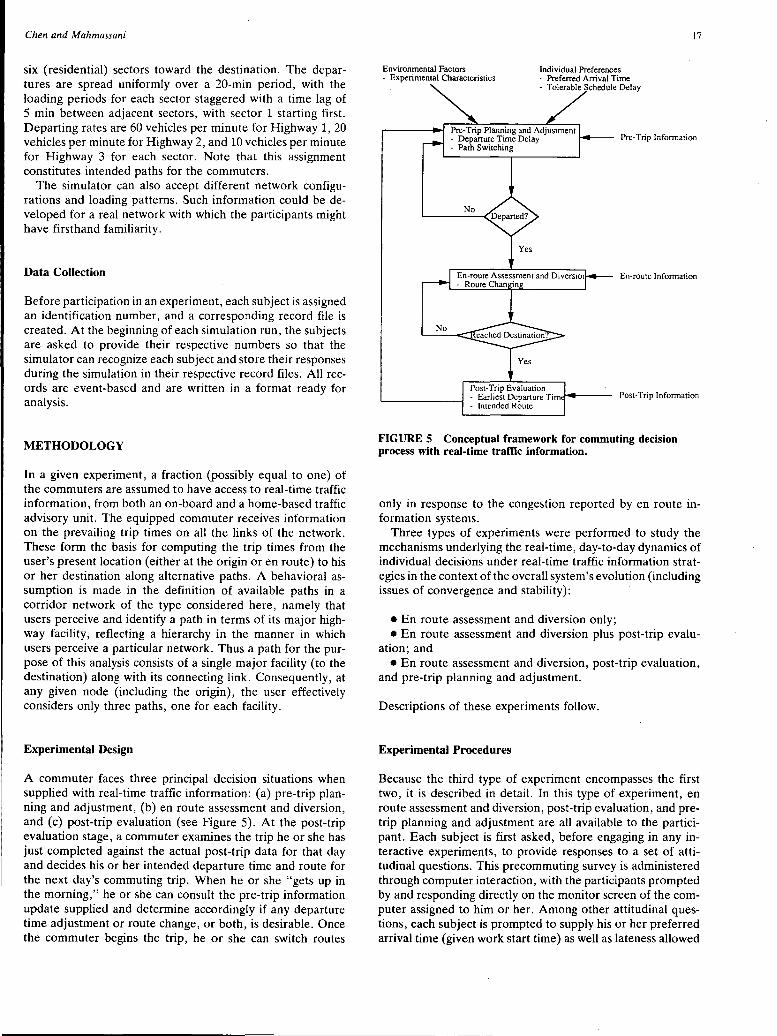
Chen and Mahmassani

six (residential) sectors toward the destination. The depar­tures are spread uniformly over a 20-min period, with the loading periods for each sector staggered with a time lag of 5 min between adjacent sectors, with sector 1 starting first. Departing rates are 60 vehicles per minute for Highway 1, 20 vehicles per minute for Highway 2, and 10 vehicles per minute for Highway 3 for each sector. Note that this assignment constitutes intended paths for the commuters.

The simulator can also accept different network configu­rations and loading patterns. Such information could be de­veloped for a real network with which the participants might have firsthand familiarity.

Data Collection

Before participation in an experiment, each subject is assigned an identification number, and a corresponding record file is created. At the beginning of each simulation run, the subjects are asked to provide their respective numbers so that the simulator can recognize each subject and store their responses during the simulation in their respective record files. All rec­ords are event-based and are written in a format ready for analysis.

METHODOLOGY

In a given experiment, a fraction (possibly equal to one) of the commuters are assumed to have access to real-time traffic information, from both an on-board and a home-based traffic advisory unit. The equipped commuter receives information on the prevailing trip times on all the links of the network. These form the basis for computing the trip times from the user's present location (either at the origin or en route) to his or her destination along alternative paths. A behavioral as­sumption is made in the definition of available paths in a corridor network of the type considered here, namely that users perceive and identify a path in terms of its major high­way facility, reflecting a hierarchy in the manner in which users perceive a particular network. Thus a path for the pur­pose of this analysis consists of a single major facility (to the destination) along with its connecting link. Consequently, at any given node (including the origin), the user effectively considers only three paths, one for each facility.

Experimental Design

A commuter faces three principal decision situations when supplied with real-time traffic information: (a) pre-trip plan­ning and adjustment, (b) en route assessment and diversion, and (c) post-trip evaluation (see Figure 5). At the post-trip evaluation stage, a commuter examines the trip he or she has just completed against the actual post-trip data for that day and decides his or her intended departure time and route for the next day's commuting trip. When he or she "gets up in the morning,'' he or she can consult the pre-trip information update supplied and determine accordingly if any departure time adjustment or route change, or both, is desirable. Once the commuter begins the trip, he or she can switch routes

17

Environmental Factors Individual Preferences - Experimental Characteristics - Preferred Arrival Time

- Tolerable Schedule Delay

Pre-Trip Information ..------~ Pre-Trip Planning and Adjustment

- Departure Time Delay - Path Switching

En-route Information

No

Post-Trip Information Post-Trip Evaluation - Earliest Departure Tim - Intended Route

FIGURES Conceptual framework for commuting decision process with real-time traffic information.

only in response to the congestion reported by en route in­formation systems.

Three types of experiments were performed to study the mechanisms underlying the real-time, day-to-day dynamics of individual decisions under real-time traffic information strat­egies in the context of the overall system's evolution (including issues of convergence and stability):

•En route assessment and diversion only; •En route assessment and diversion plus post-trip evalu­

ation; and • En route assessment and diversion, post-trip evaluation,

and pre-trip planning and adjustment.

Descriptions of these experiments follow.

Experimental Procedures

Because the third type of experiment encompasses the first two, it is described in detail. In this type of experiment, en route assessment and diversion, post-trip evaluation, and pre­trip planning and adjustment are all available to the partici­pant. Each subject is first asked, before engaging in any in­teractive experiments, to provide responses to a set of atti­tudinal questions. This precommuting survey is administered through computer interaction, with the participants prompted by and responding directly on the monitor screen of the com­puter assigned to him or her. Among other attitudinal ques­tions, each subject is prompted to supply his or her preferred arrival time (given work start time) as well as lateness allowed

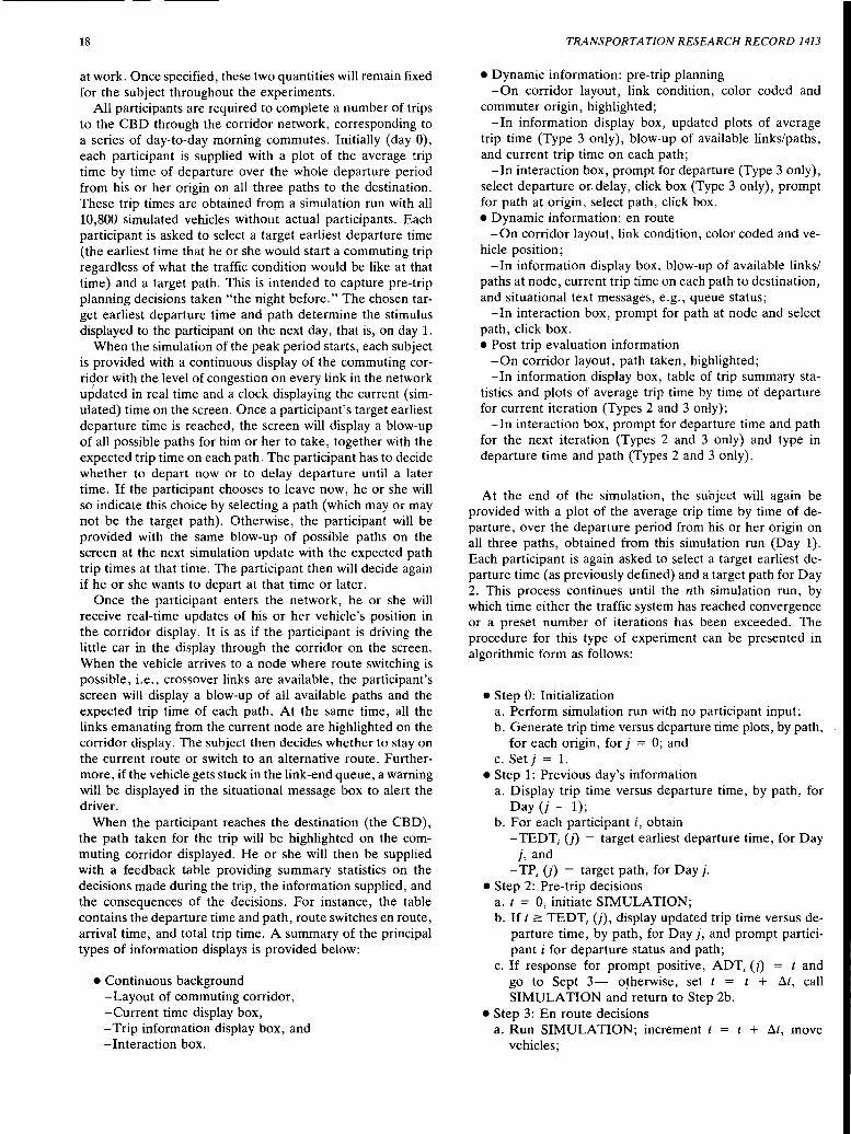
18

at work. Once specified, these two quantities will remain fixed for the subject throughout the experiments.

All participants are required to complete a number of trips to the CBD through the corridor network, corresponding to a series of day-to-day morning commutes. Initially (day 0), each participant is supplied with a plot of the average trip time by time of departure over the whole departure period from his or her origin on all three paths to the destination. These trip times are obtained from a simulation run with all 10,800 simulated vehicles without actual participants. Each participant is asked to select a target earliest departure time (the earliest time that he or she would start a commuting trip regardless of what the traffic condition would be like at that time) and a target path. This is intended to capture pre-trip planning decisions taken "the night before." The chosen tar­get earliest departure time and path determine the stimulus displayed to the participant on the next day, that is, on day 1.

When the simulation of the peak period starts, each subject is provided with a continuous display of the commuting cor­ridor with the level of congestion on every link in the network updated in real time and a clock displaying the current (sim­ulated) time on the screen. Once a participant's target earliest departure time is reached, the screen will display a blow-up of all possible paths for him or her to take, together with the expected trip time on each path. The participant has to decide whether to depart now or to delay departure until a later time. If the participant chooses to leave now, he or she will so indicate this choice by selecting a path (which may or may not be the target path). Otherwise, the participant will be provided with the same blow-up of possible paths on the screen at the next simulation update with the expected path trip times at that time. The participant then will decide again if he or she wants to depart at that time or later.

Once the participant enters the network, he or she will receive real-time updates of his or her vehicle's position in the corridor display. It is as if the participant is driving the little car in the display through the corridor on the screen. When the vehicle arrives to a node where route switching is possible, i.e., crossover links are available, the participant's screen will display a blow-up of all available paths and the expected trip time of each path. At the same time, all the links emanating from the current node are highlighted on the corridor display. The subject then decides whether to stay on the current route or switch to an alternative route. Further­more, if the vehicle gets stuck in the link-end queue, a warning will be displayed in the situational message box to alert the driver.

When the participant reaches the destination (the CBD), the path taken for the trip will be highlighted on the com­muting corridor displayed. He or she will then be supplied with a feedback table providing summary statistics on the decisions made during the trip, the information supplied, and the consequences of the decisions. For instance, the table contains the departure time and path, route switches en route, arrival time, and total trip time. A summary of the principal types of information displays is provided below:

• Continuous background -Layout of commuting corridor, -Current time display box, -Trip information display box, and -Interaction box.

TRANSPORTATION RESEARCH RECORD 1413

• Dynamic information: pre-trip planning -On corridor layout, link condition, color coded and

commuter origin, highlighted; -In information display box, updated plots of average

trip time (Type 3 only), blow-up of available links/paths, and current trip time on each path;

-In interaction box, prompt for departure (Type 3 only), select departure or delay, click box (Type 3 only), prompt for path at origin, select path, click box. • Dynamic information: en route

-On corridor layout, link condition, color coded and ve­hicle position;

- In information display box, blow-up of available links/ paths at node, current trip time on each path to destination, and situational text messages, e.g., queue status;

- In interaction box, prompt for path at node and select path, click box. • Post trip evaluation information

-On corridor layout, path taken, highlighted; -In information display box, table of trip summary sta-

tistics and plots of average trip time by time of departure for current iteration (Types 2 and 3 only);

-In interaction box, prompt for departure time and path for the next iteration (Types 2 and 3 only) and type in departure time and path (Types 2 and 3 only).

At the end of the simulation, the subject will again be provided with a plot of the average trip time by time of de­parture, over the departure period from his or her origin on all three paths, obtained from this simulation run (Day 1). Each participant is again asked to select a target earliest de­parture time (as previously defined) and a target path for Day 2. This process continues until the nth simulation run, by which time either the traffic system has reached convergence or a preset number of iterations has been exceeded. The procedure for this type of experiment can be presented in algorithmic form as follows:

• Step 0: Initialization a. Perform simulation run with no participant input; b. Generate trip time versus departure time plots, by path,

for each origin, for j = O; and c. Set j = 1.

•Step 1: Previous day's information a. Display trip time versus departure time, by path, for

Day (j - 1); b. For each participant i, obtain

-TEDT; (j) = target earliest departure time, for Day j, and

- TP; (j) = target path, for Day j. • Step 2: Pre-trip decisions

a. t = 0, initiate SIMULATION; b. If t ~ TEDT; (j), display updated trip time versus de­

parture time, by path, for Day j, and prompt partici­pant i for departure status and path;

c. If response for prompt positive, ADT; (j) = t and go to Sept 3- otherwise, set t = t + 6.t, call SIMULATION and return to Step 2b.

•Step 3: En route decisions a. Run SIMULATION; increment t = t + 6.t, move

vehicles;

Chen and Mahmassani

b. For each participant with ADT; (j) ::::; t, i. Check if at destination: if yes, go to Step 3c: other­

wise continue. ii. Check if at decision node: if yes, display trip time

(by path), prompt route choice, read user selection and/or apply default route; otherwise, continue.

iii. Return to Step 3a c. Check if t;::::: T: if yes, continue; otherwise, go to Step

3a. •Step 4: Post-trip Evaluation

a. Highlight path taken on corridor layout, b. Display table of trip summary statistics.

•Step 5: Convergence Check If convergence reached, or j > N, STOP; Otherwise, set j =

j + 1, go to Step 1.

The procedures for the other two types of experiments are similar. In Type 2 experiments, the subject's vehicle is loaded into the network at his or her specified departure time because the option to adjust the departure time in real time is un­available. In Type 1 experiments, the subject's vehicle is loaded into the network at a preassigned departure time, which may not be changed by the participant.

Experimental Factors

The interactive experiments are intended to investigate the effect of six principal factors: departure origin, background traffic, decision time constraint, rate of information update, simulation time frame, and information display strategies.

Departure Origin

Depending on his or her origin, the driver may have four, three, two, or only one opportunity for en route switching. This may affect his or her propensity to switch. Different departure origins are assigned at random to the participating subjects. Once assigned, each participant's origin remains un­changed throughout all experiments.

Background Traffic

Background traffic is the simulated traffic that interacts with the participants' vehicles in the same corridor network. There are 10,800 simulated vehicles, some of which do not switch routes because they are not equipped with traffic advisory units or their drivers do not rely on real-time information. The equipped vehicles (reflecting the particular market pen­etration scenario of interest) switch routes according to the behavioral rules described in "Path Selection and Switching Rules." The relative proportions of the two types of vehicles and the behavioral rules are under the analyst's control.

Decision Time Constraint

This is the time constraint imposed on real-time decisions. At the origin, the participant has a limited amount of time to decide if he or she will depart and .on what path. If the time

19

runs out before a response has been supplied by the partici­pant, he or she does not leave. During the trip, if the partic­ipant is faced with a route-switching decision and does not respond within the time limit, he or she will continue on the current route (default option). This time constraint can be adjusted to simulate real-life driving time constraints under various traffic conditions.

Rate of Information Update

The time between each real-time information update will be varied to observe effects on the participants' decisions as well as overall system performance. This should yield insights into what an optimal update rate might be.

Simulation Time Frame

Two versions of the interactive experiments have been de­veloped. One version performs the simulation and user in­teraction at a rate that is synchronous with real time. The other version performs the simulation and user interaction at a faster pace than real time.

Information Display Strategies

Three different display strategies are considered here. The first strategy is to supply route-based trip time information only when the subject's vehicle reaches a decision node, that is, one where there are opportunities for path switching. The second strategy is to display route-based trip time information at all points along the trip to the destination and update this information at the rate of information update as another con­trolled factor, as mentioned previously. The third strategy is to provide route-based trip time information only when re­quested by the participant, in this case by using the mouse to move the cursor to the space provided on the screen.

CONCLUDING COMMENTS

One of the principal determinants of the effectiveness of real­time traffic information systems is the user's response to this information, both in real time and over the long run. The available body of knowledge in this area is very limited and will remain rather speculative until a meaningful observa­tional basis has been developed. Laboratory-like experiments of the type described in this paper can provide a low-cost alternative for a much needed start on acquiring observations of actual tripmakers. Three unique features of the experi­mental apparatus and procedures described in this paper should be stressed: (a) the stimuli provided to the participants are generated by a traffic simulation model and are therefore both internally and externally consistent with real-world traffic con­ditions, (b) the interactive multiuser capability introduces greater realism, especially at higher market penetration lev­els, and ( c) the day-to-day aspect of the experiments addresses

20

an essential question that has often been ignored in discussions of A TIS effectiveness.

The kind of data that can be obtained from such controlled conditions provides a basis for the development of user-response models that may be used in simulation-assignment tools to evaluate network performance under real-time information. The richness of these data and the dynamic interactive nature of their sources raise challenging methodological questions in terms of analysis, particularly model specification and param­eter estimation. It is therefore necessary to advance the state­of-the-art methodologically to take advantage of such data and properly address the behavioral questions of interest. Naturally, simulators and laboratory-like experiments of the type described in this paper are not intended to totally replace actual field demonstrations and tests. Their role is to provide a relatively low cost and rapid test bed to address key fun­damental issues that are critical to further develop and deploy IVHS technologies. Insights gained from such experiments can then guide the cost-effective development of full-scale field tests. Further discussion of the role of laboratory-like exper­iments in the hierarchy of approaches for the study of complex large-scale systems is given by Mahmassani and Herman (26).

ACKNOWLEDGMENT

This paper is based on research work funded by the U.S. Department of Transportation through the Southwest Region University Transportation Center.

REFERENCES

1. Smart Highways: An Assessment of their Potential to Improve Travel. Report to the Chairman, Subcommittee on Transporta­tion, Committee on Appropriations, U.S. Senate, GAO/PEMD-91-18. General Accounting Office, 1991.

2. Intelligent Vehicle-Highway Systems (/VHS) Projects in the United States: Operational Tests and Research Activities. Office of Traffic Operations and IVHS, FHWA, U.S. Department of Transpor­tation, 1991.

3. Catling, I., and B. McQueen. Road Transport Informatics in Europe-Major Programs and Demonstrations. IEEE Trans­actions on Vehicular Technology, Vol. 40, No. 1, 1991, pp. 132-140.

4. Kawashima, H. Two Major Programs and Demonstrations in Japan. IEEE Transactions on Vehicular Technology, Vol. 40, No. 1, 1991, pp. 141-146.

5. Workshop on Intelligent Vehicles and Highway Systems-Exec­utive Summary. Mobility 2000, Dallas, Tex., 1990.

6: Advanced Driver Information Systems- Final Report of the Working Group on ADIS. Mobility 2000, Dallas, Tex., 1990.

7. Rillings, J. H., and R. J. Betsold. Advanced Driver Information Systems. IEEE Transactions on Vehicular Technology, Vol. 40, No. 1, 1991, pp. 31-40.

8. Route Guidance and In-Car Communication Systems. Road Transport Research, Organization for Economic Coordination and Development, Paris, France, 1988.

9. Mahmassani, H. S., and R. Jayakrishnan. System Performance and User Response under Real-Time Information in a Congested Traffic Corridor. Transportation Research A, Vol. 25 A, No. 5, 1991, pp. 293-307.

10. Mahmassani, H. S., and P. S. Chen. Comparative Assessment of Origin-Based and En-Route Real-Time Information under Alternative User Behavior Rules. In Transportation Research Record 1306, TRB, National Research Council, Washington, D.C., 1991, pp. 69-81.

TRANSPORTATION RESEARCH RECORD 1413

11. Tsuji, H., R. Takahanshi, H. Kawashima, and Y. Yamamoto. ·A Stochastic Approach for Estimating the Effectiveness of a Route Guidance System and Its Related Parameters. Transpor­tation Science, Vol. 19, No. 4, 1985, pp. 333-351.

12. LeBlanc, L. J. Telecommunication Network Configuration for In-Vehicle Route-Guidance Systems. Proc., U.S.-Italian Joint Seminar on Urban Traffic Networks: Dynamic Control and Flow Equilibrium, Capri, Italy, 1989, pp. 209-282.

13. Koutsopoulos, H. N., and T. Lotan. Motorist Information Sys­tems and Recurrent Traffic Congestion: A Sensitivity Analysis of Expected Benefits. In Transportation Research Record 1281, TRB, _National Research Council, Washington, D.C., 1990, pp. 148-159.

14. Dingus, T. A., J. F. Antin, M. C. Hulse, and W. W. Wierwille. Attentional Demand Requirements of an Automobile Moving­Map Navigation System. Transportation Research A, Vol. 23A, No. 4, 1989, pp. 301-315.

15. Parkes, A. M., M. C. Ashby, and S. H. Fairclough. The Effects of Different In-Vehicle Route Informatioff Displays on Driver Behavior. Proc., Vehicle Navigation and Information Systems Conference, Vol. 1. Society of Automotive Engineers, Inc., Dear­born, Mich., 1991, pp. 61-70.

16. Walker, J., E. Alicandri, C. Sedney, and K. Roberts. In-Vehicle Navigation Devices: Effects on the Safety of Driver Performance. Proc., Vehicle Navigation and Information Systems Conference, Vol. 1. Society of Automotive Engineers, Inc., Dearborn, Mich., 1990, pp. 499-525.

17. Shirazi, E., S. Anderson, and J. Stesney. Commuters' Attitudes Toward Traffic Information Systems and Route Diversion. In Transportation Research Record 1168, TRB, National Research Council, Washington, D.C., 1988.

18. Haselkorn M., J. Spyridakis, and W. Barfield. Surveying Com­muters to Obtain Functional Requirements for the Design of a Graphic-Based Traffic Information System. Proc., Vehicle Nav­igation and Information Systems Conference, Vol. 2, Society of Automotive Engineers, Inc., Dearborn, Mich., 1991, pp. 1,041-1,044.

19. Khattak, A. J., J. L. Schofer, and F. S. Koppelman. Factors Influencing Commuters' En Route Diversion Behavior in Re­sponse to Delay. In Transportation Research Record 1318, TRB, National Research Council, Washington, D.C., 1991.

20. Khattak, A. J., F. S. Koppelman, and J. L. Schofer. Stated Pref­erences for Investigating Commuters' Diversion Propensity. Presented at 71st Annual Meeting of the Transportation Research Board, Washington, D.C., 1992.

21. Bonsall, P. W., and T. Parry. Using an Interactive Route-Choice Simulator to Investigate Drivers' Compliance with Route Guid­ance Advice. In Transportation Research Record 1306, TRB, National Research Council, Washington, D.C., 1991, pp. 59-68.

22. Allen, R. W., A. C. Stein, T. J. Rosenthal, D. Ziedman, J. F. Torres, and A. Halati. A Human Factors Simulation Investiga­tion of Driver Route Diversion and Alternative Route Selection Using In-Vehicle Navigation Systems. Proc., Vehicle Navigation and Information Systems Conference, Vol. 1. Society of Auto­motive Engineers, Inc., Dearborn, Mich., 1991, pp. 9-26.

23. Adler, J. L., W.W. Recker, and M. G. McNally. A Conflict Model and Interactive Simulator (FASTCARS). Presented at 71st Annual Meeting of the Transportation Research Board, Washington, D.C., 1992.

24. Chen, P. S., and H. S. Mahmassani. Reliability of Real-Time Information Systems for Route Choice Decisions in a Congested Traffic Network: Some Simulation Experiments. Proc., Vehicle Navigation and Information Systems Conference, Vol. 2, Society of Automotive Engineers, Inc., Dearborn, Mich., 1991, pp. 849-856.

25. Mahmassani, H. S., and P. S. Chen. An Investigation of the Reliability of Real-Time Information for Route Choice Decision in a Congested Traffic System. Presented at 71st Annual Meeting of the Transportation Research Board, Washington, D.C., 1992.

26. Mahmassani, H. S., and R. Herman. Interactive Experiments for the Study of Tripmaker Behavior Dynamics in Congested Commuting Systems. In Developments in Dynamic and Activity Based Approaches to Travel Analysis (P. Jones, ed.), Gower, Aldershot, England, 1990, pp. 272-298.

Chen and Mahmassani

27. Johnson, E. F., and K. Reichard. X Window: Applications Pro­gramming. Management Information Sources, Inc., Portland, Oreg., 1989.

28. Norman, D. A. The Psychology of Everyday Things. Basic Books, Inc., New York, 1988.

29. Rubinstein, R., and H. M. Hersh. The Human Factor: Designing Computer Systems for People. Digital Press, Bedford, Mass., 1984.

30. Kahneman, D. Attention and Effort. Prentice-Hall, Inc., Engle­wood Cliffs, N.J., 1973.

31. Jayakrishnan, R. In-Vehicle Information Systems for Network Traffic Control: A Simulation Framework to Study Alternative Guidance Strategies. Ph.D. dissertation. University of Texas, Austin, Tex., 1991.

21

32. Mahmassani, H. S., T. Hu, and R. Jayakrishnan. Dynamic Traffic Assignment and Simulations for Advanced Network Information. Presented at 2nd International Capri Seminar on Urban Traffic Networks, Capri, Italy, 1992.

The views expressed here are solely those of the authors and do not necessarily reflect those of the sponsoring agency.

Publication of this paper sponsored by Committee on Traveler Be­havior and Values.

22 TRANSPORTATION RESEARCH RECORD 1413

Stated Preference Approach to Modeling the Adoption of Telecommuting

ADRIANA BERNARDINO, MOSHE BEN-AKIVA, AND lLAN SALOMON

Many researchers have suggested the potential use of telecom­muting as a substitute for travel to reduce traffic congestion, energy consumption, and air pollution. The effectiveness of this working arrangement as a strategy to address these policy issues, however, will depend on the level of adoption and on the impacts of usage on individuals' travel behavior. This paper discusses the process of individuals' adoption of telecommuting, given that the alternative is made available by the employer. A review of the relevant research concerning individuals and the process of adop­tion of telecommuting is presented. On the basis of the state of the art, a framework to model this process is proposed. An em­pirical study conducted to demonstrate the proposed framework is described. The implications of the main findings of this study policy design are analyzed and directions for further research are suggested.

Many researchers have suggested the potential use of tele­commuting as a substitute for travel to reduce traffic conges­tion, energy consumption, and air pollution. This expectation is derived from four major trends: innovations in the area of information technology (IT), the increasing social cost of transportation, the transition to the "information economy," and changes in individuals' lifestyles.

Developments in information technology have significantly reduced the costs of terminal equipment and increased their capabilities. The introduction of fiber optics and microwaves represents a potential growth in terms of capacity and speed of data transmission. Many IT applications are now being devel­oped to improve individuals' and groups' interactions, relax­ing physical and temporal constraints on activity performance.

These innovations significantly reduce coordination costs, leading organizations to a restructuring process that continues to involve more value-added partnership and ad hoc team­work instead of rigid, hierarchical structures. Consequently, the accessibility of employees through a communication net­work becomes much more important than their physical pres­ence in the office, which may encourage the adoption of telecommuting.

Simultaneously, policy makers' interest in telecommuting is significantly growing, as shown by the recent, increasing level of investments made in demonstration projects. In addition to its potential to reduce private and social transportation costs at a low investment level by government, telecommuting can also address issues such as regional development, oppor­tunities for disabled persons, and emergency preparedness, among others.

A. Bernardino and M. Ben-Akiva, Department of Civil and Envi­ronmental Engineering, Massachusetts Institute of Technology, 77 Massachusetts Avenue, Cambridge, Mass. 02319. I. Salomon, De­partment of Geography, Har Hazoffim, Hebrew University, Jeru­salem, Israel.

Nevertheless, some transportation and telecommunications planners have questions still to be answered. There are in­dications that telecommuting is gaining ground in the United States and Europe. However, the assessments of the current number of telecommuters, as well as the current forecasts of telecommuting and its impacts in terms of demand for infra­structure and services, vary widely. The variations are due to inconsistent definitions and inappropriate forecasting tech­niques as well as different assumptions about the nature of the behavioral responses to the availability of this option.

The objective of this study is to take one further step in the direction of understanding telecommuting, beyond most efforts conducted to date. This study involved the develop­ment of a model of the decision to adopt telecommuting by the individual.

The remainder of this paper is organized in four sections. The section on Previous Research presents a review of the research concerning individuals and the process of adopting telecommuting. The section on Modeling Framework proposes a framework to model the adoption process. The Pilot Study and Conclusions sections describe and discuss an empirical study conducted to demonstrate the proposed framework.

PREVIOUS RESEARCH

Research relevant to the process of adopting telecommuting by the individual can be broadly divided into two main streams: one that emphasizes the sociological aspects of this new work­ing arrangement and another that focuses on the impacts of telecommuting on travel behavior.

Sociological research describes some characteristics of in­dividuals, their households, ·and their environments that may be relevant to the adoption of telecommuting, as well as the impacts of adoption of this working arrangement on telecom­muters. Travel behavior research analyzes individuals' pat­terns of usage of the transportation system once telecom­muting is adopted.

Characteristic of the research on telecommuting is the fact that studies fall short of taking a comprehensive perspective, usually remaining within traditional disciplinary lines. The main studies in both of the two major directions of research follow.

Sociological Research

Sociological research can be further divided into characteri­zation of telecommuters profiles and impacts of telecommut­ing adoption on individuals.

Bernardino et al.

Characterizations of Telecommuters' Profiles

Olson (J), Olson and Primps (2), and Pratt (3), based on analyses of work-at-home pilot programs of various organi­zations, identified telecommuters as (a) male managers or professionals who perceive more value in part-time integra­tion of work and family than career advancement, (b) full­time female clerical workers who have child-care responsi­bilities or are seeking to increase income by reducing personal expenses, and (c) managerial and professional mothers who want to nurture young children without completely falling behind in their careers.

Kraut and Grambsch ( 4), based on a statistical analysis of 1980 census work-at-home data, observed that telecommuters were likely to belong to groups that experience social or phys­ical constraints to their mobility. This finding, however, may not be representative of actual telecommuters because the definition of work-at-home in the census is much broader than that of telecommuting.

Bailyn (5), analyzing an organization in the United King­dom, found that telecommuters tend to value interesting work, family life, and leisure time more than pursuing a career. Their counterparts, the office workers who do not telecom­mute, are more career oriented and value status, prestige, and success more than family life, flexibility, and merely main­taining skills.

The author also identified a "traditional" home-based ori­entation among female telecommuters, who were more in­terested in home and family than in career goals. Male tele­commuters, on the other hand, perceived some value in work but had given priority to their preferred lifestyle and a bal­anced life over career and achievement.

Christensen (6) and Olson (7) proposed that only managers and professional workers will decide to work at home on the basis of their personal preferences. Clerical employees will work under this arrangement due to family demands or to low income levels.

These studies lead to the hypotheses that alternative life­styles and socioeconomic constraints may be significant fac­tors in the decision to adopt telecommuting. They also suggest the hypothesis that telecommuters will either be in the po­sition of bargaining for their working arrangement or, having no alternative, being eventually exploited.

Impacts of Adopting Telecommuting on Individuals

Telecommuting may be quite a radical change from the rou­tine work patterns. Work is the main activity around which other activities are organized. Thus a change in the work arrangement may have far-reaching impacts on the total. ac­tivity patterns of individuals and their households. The ex­pected impacts on individuals are likely to affect their like­lihood of adopting telecommuting. Moreover, the likelihood that others will adopt telecommuting is also a factor that may influence this decision.

Through interviews with supervisors, Pratt. (3) identified some categories of white collar employees who had either returned to the office full time or stopped working after re­jecting home telework. The main categories identified were (a) single men and women whose social life centered on office contacts, (b) handicapped workers who found it physically

23

impossible to work long hours at a terminal, (c) workers whose families objected to their presence at home, ( d) individuals who were not self-disciplined enough to perform their jobs without supervision, and ( e) workers whose off-site produc­tivity could not be easily measured by their supervisors.

In a study evaluating changes in home computer use, Vi­talari et al. (8) concluded that computers at home were used mostly for work and had the impact of decreasing the time spent with family and friends and increasing the time spent alone, leading to social isolation. Kraut (9) concluded that the experience with computer owners to date shows that in­dividuals use home computers to work extra, generally non­paid, hours. Bailyn (5) suggests that both "workaholism" and exploitation of workers by organizations may be observed in telecommuting.

Reviewing Christensen's work, Bailyn also pointed out the findings that telecommuting and child care can be combined only with difficulty. When adopting this option, male profes­sionals experienced improvements in family life, whereas the opposite was experienced by female clerical workers with re­placeable skills. Olson (7) also confirmed that women working at home felt constant stress and pressure from both work and family demands, with little time left for themselves or for leisure.

In a review of four telecommuting experiments conducted in Japan, Spinks (10) identifies the main work-related prob­lems to be a lack of concise job descriptions as well as a lack of time-management and self-supervisory skills. Most indi­viduals agreed that flexibility to work according to ones' bio­rhythm was more productive and generated a greater sense of creativity, but a lack of motivation in the initial stages led to longer working hours closer to deadlines.

An interesting aspect noted in one of the experiments was that, for cultural re~sons, some individuals did not feel com­fortable about the possibility of having the whole family to­gether frequently.

The absence of a commute was positively regarded by most telecommuters, as well as the possibility of working in casual clothing. However, by working and living under the same roof, some telecommuters never experienced the feeling of being completely "off duty."

These findings lead to the conclusion that it is necessary to consider job and commuting characteristics, as well as indi­viduals' personalities, attitudes, and cultural values, when evaluating the potential telecommuting adoption.

Telecommuting, Travel Behavior, and the Transportation System

Salomon (11), Nilles (12), and Mokhtarian (13) have dis­cussed the expected impacts of telecommuting on travel be­havior, and the main hypotheses formulated from these dis­cussions can be classified as short-term or long-term hypotheses.

The most immediate expected result is a reduction in the number of peak-hour trips due to the reduction of commutes. A shift of trip time to off-peak hours is also expected. Non­work trip destinations may be expected to be closer to home, allowing for a shift to nonmotorized transportation modes. On the other hand, carpools may be interrupted, requiring individuals to drive alone and generating more trips as a re­sult. A· reassignment of activities may be observed in tele-

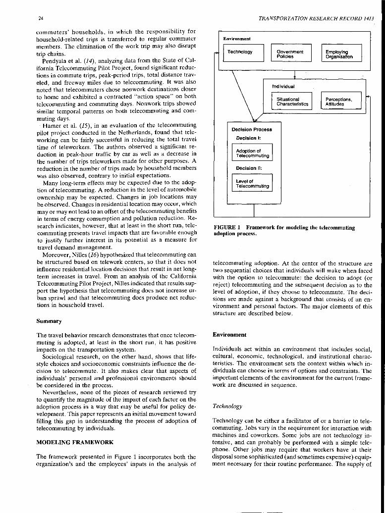
24

commuters' households, in which the responsibility for household-related trips is transferred to regular commuter members. The elimination of the work trip may also disrupt trip chains.

Pendyala et al. (14), analyzing data from the State of Cal­ifornia Telecommuting Pilot Project, found significant reduc­tions in commute trips, peak-period trips, total distance trav­eled, and freeway miles due to telecommuting. It was also noted that telecommuters chose nonwork destinations closer to home and exhibited a contracted "action space" on both telecommuting and commuting days. Nonwork trips showed similar temporal patterns on both telecommuting and com­muting days.

Hamer et al. (15), in an evaluation of the telecommuting pilot project conducted in the Netherlands, found that tele­working can be fairly successful in reducing the total travel time of teleworkers. The authors observed a significant re­duction in peak-hour traffic by car as well as a decrease in the number of trips teleworkers made for other purposes. A reduction in the number of trips made by household members was also observed, contrary to initial expectations.

Many long-term effects may be expected due to the adop­tion of telecommuting. A reduction in the level of automobile ownership may be expected. Changes in job locations may be observed. Changes in residential location may occur, which may or may not lead to an offset of the telecommuting benefits in terms of energy consumption and pollution reduction. Re­search indicates, however, that at least in the short run, tele­commuting presents travel impacts that are favorable enough to justify further interest in its potential as a measure for travel demand management.

Moreover, Nilles (16) hypothesized that telecommuting can be structured based on telework centers, so that it does not influence residential location decisions that result in net long­term increases in travel. From an analysis of the California Telecommuting Pilot Project, Nilles indicated that results sup­port the hypothesis that telecommuting does not increase ur­ban sprawl and that telecommuting does produce net reduc­tions in household travel.

Summary

The travel behavior research demonstrates that once telecom­muting is adopted, at least in the short run, it has positive impacts on the transportation system.

Sociological research, on the other hand, shows that life­style choices and socioeconomic constraints influence the de­cision to telecommute. It also makes clear that aspects of individuals' personal and professional environments should be considered in the process.

Nevertheless, none of the pieces of research reviewed try to quantify the magnitude of the impact of each factor on the adoption process in a way that may be useful for policy de­velopment. This paper represents an initial movement toward filling this gap in understanding the process of adoption of telecommuting by individuals.

MODELING FRAMEWORK

The framework presented in Figure 1 incorporates both the organization's and the employees' inputs in the analysis of

TRANSPORTATION RESEARCH RECORD 1413

Environment

Technology

Decision Process

Decision I:

Adoption of Telecommuting

Decision II:

Level of Telecommuting

Government Policies

Individual

Situational Characteristics

Employing Organization

Perceptions, Attitudes

FIGURE 1 Framework for modeling the telecommuting adoption process.

telecommuting adoption. At the center of the structure are two sequential choices that individuals will make when faced with the option to telecommute: the decision to adopt (or reject) telecommuting and the subsequent decision as to the level of adoption, if they choose to telecommute. The deci­sions are made against a background that consists of an en­vironment and personal factors. The major elements of this structure are described below.

Environment

Individuals act within an environment that includes social, cultural, economic, technological, and institutional charac­teristics. The environment sets the context within which in­dividuals can choose in terms of options and constraints. The important elements of the environment for the current frame­work are discussed in sequence.

Technology

Technology can be either a facilitator of or a barrier to tele­commuting. Jobs vary in the requirement for interaction with machines and coworkers. Some jobs are not technology in­tensive, and can probably be performed with a simple tele­phone. Other jobs may require that workers have at their disposal some sophisticated (and sometimes expensive) equip­ment necessary for their routine performance. The supply of

Bernardino et al.

such technologies at the individuals' home raises a number of questions regarding technological feasibility, costs, and other administrative issues.

Government Policies

Governmental entities are initiating policies to reduce trans­portation's social costs and to encourage organizations to adopt programs to decrease the number of trips made by their em­ployees. In some areas, these policies include an extra bonus for trip reductions obtained by telecommuting. By using these types· of regulatory devices, government can exert some in­fluence on the level of adoption of telecommuting. On the other hand, other government agencies are involved in for­mulating policies designed to protect workers; such policies may not be consistent with those encouraging telecommuting.

Employer

The employing organization's decision to make telecommut­ing available is a necessary condition for adoption to take place. This decision is a function of the organization's char­acteristics and of managers' perceptions and attitudes.

Relevant organization characteristics are the composition of the labor force, organizational costs, and organizational structure. The characteristics of the labor force may have an impact not only on the decision to offer telecommuting as an option, but also on the characteristics of the proposed pro­gram. It may be expected, for example, that programs offered to professional workers will be more flexible than those of­fered to clerical employees.

Organization costs may also be relevant to the adoption process. Significant savings may be obtained by reduced re­quirements of office and parking space. Telecommuting may also decrease absenteeism, sick leave, and turnover rates, and avoid relocation costs. On the other hand, the costs of im­plementing and operating a telecommuting program may be prohibitive.

The relevance of the organizational structure to the adop­tion process refers basically to the level of interaction among individuals, sectors, and departments and to the media used to perform this interaction. Structures that require a high level of interaction may have some difficulty in functioning with telecommuting. However, if most of this interaction is per­formed by means of telecommunication media, telecommut­ing may actually be favored.

Managers' perceptions and attitudes affect the organiza­tion's position with regard to telecommuting programs. Also, the message sent by the manager to the individual employee affects the way in which the individual preceives the program. There is much evidence that at present, many managers do not support telecommuting because they fail to understand how they can manage a remote work force (7). Other man­agers see a great potential in telecommuting as a measure to increase productivity.

The result of the decision made by the organization is the definition of the working arrangement characteristics. Con­sidering organizational characteristics and managers' attitudes and perceptions, a choice is made about whether to make

25

telecommuting available. Telecommuting, however, is not a single unified arrangement. In fact, the concept includes a wide variety of arrangements with the common characteristics that work is performed at a remote location, and, from a transportation perspective, that travel patterns are altered (13). Combinations of the attributes described below char­acterize the telecommuting programs that may be available to employees and directly influence the adoption decision.

Formality Telecommuting can be an informal arrange­ment between the employer and the employee, or a formal agreement. Some organizations currently institutionalizing telecommuting require employees and supervisors to sign a document on the agreed conditions. Individuals may be more willing to adopt institutionalized arrangements because this formalization may be interpreted as a commitment by the organization. On the other hand, individuals may assume in­formal arrangements to be more flexible and thus prefer that situation.

Form There are currently two main forms of telecom­muting: home-based and remote work centers. In the home­based form, employees work full- or part-time at home and report to a central, remote office. In the remote work center, employees work full- or part-time in a facility that is closer to their home than the office to which they report. At present, there is little documented experience with remote centers. Home-based telecommuting has the advantage of requiring no trips and providing more time for family interaction. On the other hand, remote centers involve a shorter trip than that to the central office, yet providing a buffer between home and office. These centers also provide greater possibilities for socialization as well as better infrastructure and a more well­defined liability context.

Flexibility Some telecommuting programs may have a rigid schedule, determining the number of days or days of the week when telecommuting is allowed. Other programs, however, can be flexible, leaving the schedule for the employee to decide and requiring only that the employee be in the office for one or one half day per week, or be accessible through telephone or computer during certain hours of the day. It is reasonable to expect that employees will prefer more flexible arrangements because flexibility is considered one of the greatest advantages of telecommuting.

Employment Conditions In recent telecommuting exper­imental projects, mainly those totally or partially funded by the government, it has been suggested that no distinction be made concerning salary and benefits between commuters and telecommuters. This is, however, not necessarily the common practice. In fact, uneven patterns of working conditions have been observed, associated with the scope of telework, orga­nizational purposes for introduction of the program, type of work, and legal aspects of the telework. Telecommuters can be treated as employees or contractors, can be paid by the task or by the hour, and can receive all regular benefits or

26

none of them. Wage rates can be lower, higher, or the same as those for regular commuters.

Fixed and Operating Costs In both home-based and re­mote work center telecommuting arrangements, the equip­ment to be used can be provided by the employee or the employer, or shared between the two parties. Similarly, main operating costs, such as phone bills, may be paid by either one of the parties or otherwise shared.

Liability Questions of liability for the equipment, infor­mation, and even the health and safety of the employee must be defined for this new form of working arrangement, par­ticularly for home-based telecommuting. If the employers bear responsibility, then they may require the right of on-site in­spection visits.

Individuals' Characteristics

The individuals' characteristics that affect the decision to telecommute include two major elements: the individuals' situational characteristics and the individuals' attitudes and perceptions.

Individuals' Situational Characteristics

Individuals' situational characteristics can be divided into three main groups: job, commuting, and socioeconomic and de­mographic characteristics.

Job characteristics involve the level of face-to-face inter­action demanded by the job and the type of equipment re­quired to accomplish the tasks. These requirements may rep­resent a set of binding constraints to telecommuting.

Commuting characteristics are expected to have a signifi­cant influence on individuals' decisions to telecommute. Long commuting times, high levels of congestion, and inconven­ience associated with travel may increase the attractiveness of telecommuting.

Socioeconomic and demographic characteristics may also affect the individuals' decision to adopt telecommuting. Gender­based roles, presence of children or adults who need spe­cial care, household income, or level of education are ex­pected to contain relevant information and may be used as a basis for market segmentation in forecasting the demand for telecommuting.

Individuals' Perceptions and Attitudes

Individuals' attitudes toward telecommuting in general, and toward specific programs in particular, will influence the de­cision of whether to consider or to adopt an arrangement. Individuals who do not understand the concept of telecom­muting may not perceive it as an viable alternative. Individuals who are career oriented may prefer to work in the central office, while those who are family oriented may prefer to telecommute.

TRANSPORTATION RESEARCH RECORD 1413

Adopting Telecommuting: Decision Structure

The process of the adoption of telecommuting involves two main decisions by the employee. Based on the working ar­rangements offered, attitudes, perceptions, and socioeco­nomic and demographic characteristics, individuals decide whether to telecommute. This is not a daily decision of whether to telecommute or to drive to work, but a long-term choice of accepting certain conditions in exchange for some benefits. Individuals may be able to move in and out of this condition depending on the characteristics of the arrangement.

Once telecommuting is adopted, individuals must decide how much telecommuting to do. In some cases, the intensity of telecommuting may be predetermined and consequently part of the first decision. Ho!,vever, more likely is the situation in which the individual has the flexibility to choose the level of telecommuting, which then becomes a short-term decision.

PILOT STUDY

To obtain some insights into the applicability of the proposed framework, a pilot study was conducted. This study is dis­cussed next.

Data Collection

The pilot study was based on a survey of a group of individuals' preferences concerning hypothetical telecommuting scena­rios, that is, stated preference data. The major advantage of this type of data is that scenarios can be elaborated on based on orthogonal design, and models estimated from this data set can elicit information on trade-offs among attributes that may not be clear from revealed preference data. Nevertheless, purely stated preference-based models present many validity problems, originating in the decision protocols adopted by the respondents, imperfect descriptions of alternatives, and omission of situational constraints. They are, therefore, of little or no value for predicting demand, unless they can be validated by revealed preference data. This aspect should be clear during the analysis of the results.

Survey

The survey questionnaire was divided into two parts. Part 1 contained questions about the respondents' job, commuting and demographic characteristics, communication patterns within the organization, the availability and characteristics of the telecom­muting program in the respondent's organization, respondent's attitudes towards telecommuting, and perceptions of main bar­riers to a broader adoption within the organization. Part 2 presented a series of telecommuting programs and asked the respondents about their willingness to telecommute if each one of those programs were offered by the organization.

The survey was advertised in eight USENET newsgroups, requiring participants. These groups were selected on the ba­sis of the contents of their ongoing discussions and were all expected to be interested in the telecommuting issue. There­fore, this is a convenience sample. To qualify as respondents, these individuals had to be employees whose jobs could be

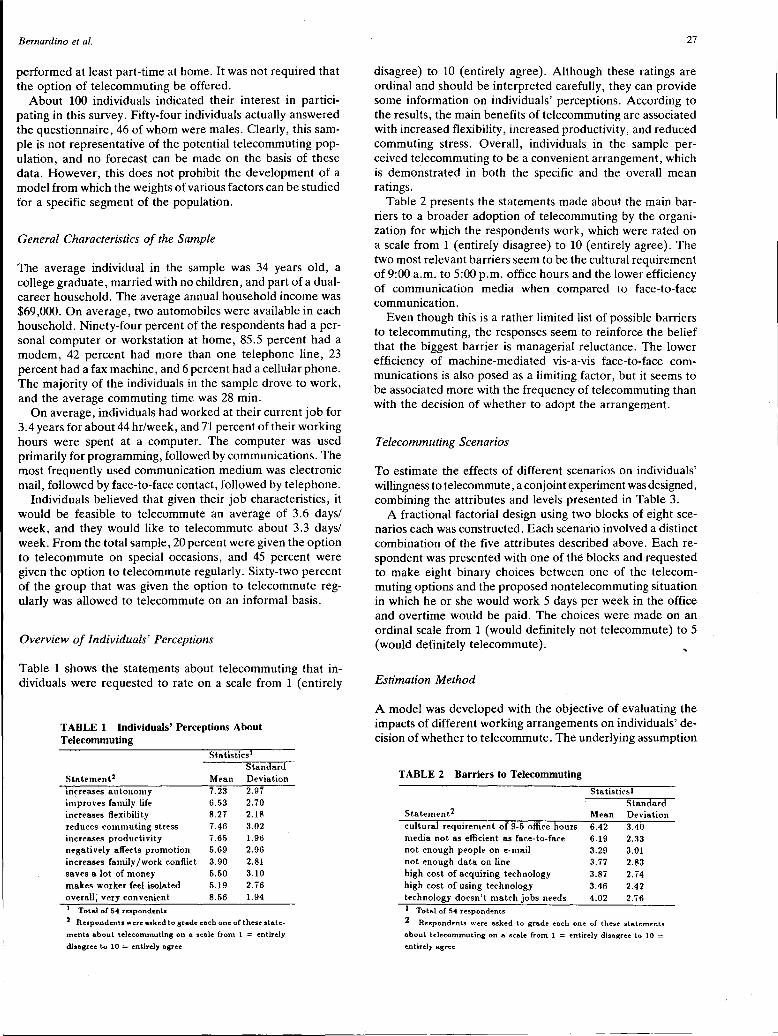
Bernardino et al.

performed at least part-time at home. It was not required that the option of telecommuting be offered.

About 100 individuals indicated their interest in partici­pating in this survey. Fifty-four individuals actually answered the questionnaire, 46 of whom were males. Clearly, this sam­ple is not representative of the potential telecommuting pop­ulation, and no forecast can be made on the basis of these data. However, this does not prohibit the development of a model from which the weights of various factors can be studied for a specific segment of the population.

General Characteristics of the Sample

The average individual in the sample was 34 years old, a college graduate, married with no children, and part of a dual­career household. The average annual household income was $69,000. On average, two automobiles were available in each household. Ninety-four percent of the respondents had a per­sonal computer or workstation at home, 85.5 percent had a modem, 42 percent had more than one telephone line, 23 percent had a fax machine, and 6 percent had a cellular phone. The majority of the individuals in the sample drove to work, and the average commuting time was 28 min.

On average, individuals had worked at their current job for 3.4 years for about 44 hr/week, and 71 percent of their working hours were spent at a computer. The computer was used primarily for programming, followed by communications. The most frequently used communication medium was electronic mail, followed by face-to-face contact, followed by telephone.

Individuals believed that given their job characteristics, it would be feasible to telecommute an average of 3.6 days/ week, and they would like to telecommute about 3.3 days/ week. From the total sample, 20 percent were given the option to telecommute on special occasions, and 45 percent were given the option to telecommute regularly. Sixty-two percent of the group that was given the option to telecommute reg­ularly was allowed to telecommute on an informal basis.

Overview of Individuals' Perceptions

Table 1 shows the statements about telecommuting that in­dividuals were requested to rate on a scale from 1 (entirely

TABLE 1 Individuals' Perceptions About Telecommuting

St.a tis tics Standard

Statement2 Mean Deviation increases autonomy 7.23 2.97 improves family life 6.53 2.70 increases flexibility 8.27 2.18 reduces commuting stress 7.46 3.02 increases productivity 7.65 1.96 negatively affects promotion 5.69 2.96 increases family /work c.onftict 3.90 2.81 saves a lot of money 5.50 3.10 makes worker feel isolated 5.19 2.76 overall; very convenient 8.56 1.94 1 Total of 54 respondents 2 Respondents were asked to grade each one of these state­

ments about telecommuting on a scale from 1 = entirely

disagree to 10 = entirely agree

27

disagree) to 10 (entirely agree). Although these ratings are ordinal and should be interpreted carefully, they can provide some information on individuals' perceptions. According to the results, the main benefits of telecommuting are associated with increased flexibility, increased productivity, and reduced commuting stress. Overall, individuals in the sample per­ceived telecommuting to be a convenient arrangement, which is demonstrated in both the specific and the overall mean ratings.

Table 2 presents the statements made about the main bar­riers to a broader adoption of telecommuting by the organi­zation for which the respondents work, which were rated on a scale from 1 (entirely disagree) to 10 (entirely agree). The two most relevant barriers seem to be the cultural requirement of 9:00 a.m. to 5:00 p.m. office hours and the lower efficiency of communication media when compared to face-to-face communication.

Even though this is a rather limited list of possible barriers to telecommuting, the responses seem to reinforce the belief that the biggest barrier is managerial reluctance. The lower efficiency of machine-mediated vis-a-vis face-to-face com­munications is also posed as a limiting factor, but it seems to be associated more with the frequency of telecommuting than with the decision of whether to adopt the arrangement.

Telecommuting Scenarios

To estimate the effects of different scenarios on individuals' willingness to telecommute, a con joint experiment was designed, combining the attributes and levels presented in Table 3.

A fractional factorial design using two blocks of eight sce­narios each was constructed. Each scenario involved a distinct combination of the five attributes described above. Each re­spondent was presented with one of the blocks and requested to make eight binary choices between one of the telecom­muting options and the proposed nontelecommuting situation in which he or she would work 5 days per week in the office and overtime would be paid. The choices were made on an ordinal scale from 1 (would definitely not telecommute) to 5 (would definitely telecommute).

Estimation Method

A model was developed with the objective of evaluating the impacts of different working arrangements on individuals' de­cision of whether to telecommute. The underlying assumption

TABLE 2 Barriers to Telecommuting

Statement2

Statisticsl Standard

Mean Deviation cultural requirement of 9-5 office hours 6.42 3.40 media not as effident as face-to-face 6.19 2.33 not enough people on e-mail 3.29 3.01 not enough data on line 3.77 2.83 high cost of acquiring technology 3.87 2.74 high cost of using technology 3.46 2.42 technology doesn't match jobs needs 4.02 2.76 1 Total of 54 respondents

2 Respondents were asked to grade each one of these stl\tcmcnt.s

about telecommuting on a scale from 1 = entirely disl\gree to 10 = entirely l\gree

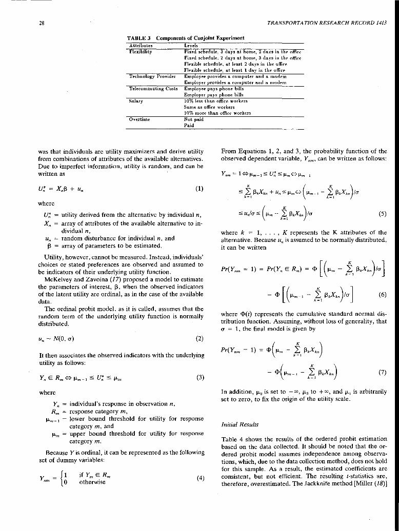
28 TRANSPORTATION RESEARCH RECORD 1413

TABLE 3 Components of Conjoint Experiment Attributes Levels Flexibility Fi~ed schedule, 3 days at home, 2 days in the office

Fixed schedule, 2 days at home, 3 days in the office Flexible schedule, at least 2 clays in the office Flexible schedule, at least 1 day in the office

Technology Provider Employee provides a computer and a modem Employer provides a computer and a modem

Telecommuting Costs Employee pays phone bills Employer pays phone bills

Salary 103 less than office workers Same as office workers 103 more than office workers

Overtime Not paid Paid

was that individuals are utility maximizers and derive utility from combinations of attributes of the available alternatives. Due to imperfect information, utility is random, and can be written as

(1)

where

u~ utility derived from the alternative by individual n, xn array of attributes of the available alternative to in­

dividual n, un = random disturbance for individual n, and

J3 = array of parameters to be estimated.

Utility, however, cannot be measured. Instead, individuals' choices or stated preferences are observed and assumed to be indicators of their underlying utility function.

McKelvey and Zavoina (17) proposed a model to estimate the parameters of interest, J3, when the observed indicators of the latent utility are ordinal, as in the case of the available data.

The ordinal probit model, as it is called, assumes that the random term of the underlying utility function is normally distributed.

Un - N(O, CT) (2)

It then associates the observed indicators with the underlying utility as follows:

(3)

where

Yn individual's response in observation n, Rm response category m,

µm _ 1 lower bound threshold for utility for response category m, and

µm = upper bound threshold for utility for response category m.

Because Y is ordinal, it can be represented as the following set of dummy variables:

if Ym E Rm otherwise

(4)

From Equations 1, 2; and 3, the probability function of the observed dependent variable, Ynm• can be written as follows:

"',t, 13.X .. + u""' µm¢> (µm-• - ,t, 13,x,}"

$ Unfcr $ ( µm - ktI ~kxkn) /a (5)

where k = 1, ... , K represents the K attributes of the alternative. Because un is assumed to be normally distributed, it can be written

1)

where <l>(t) represents the cumulative standard normal dis­tribution function. Assuming, without loss of generality, that CT = 1, the final model is given by

1) (+m - ,t, 13,X,")

- <I> ( µm- • ,t, 13,Xk") (7)

In addition, µ 0 is set to - oo, µ 5 to + oo, and µ 1 is arbitrarily set to zero, to fix the origin of the utility scale.

Initial Results

Table 4 shows the results of the ordered probit estimation based on the data collected. It should be noted that the or­dered probit model assumes independence among observa­tions, which, due to the data collection method, does not hold for this sample. As a result, the estimated coefficients are consistent, but not efficient. The resulting (-statistics are, therefore, overestimated. The Jackknife method [Miller (18)]

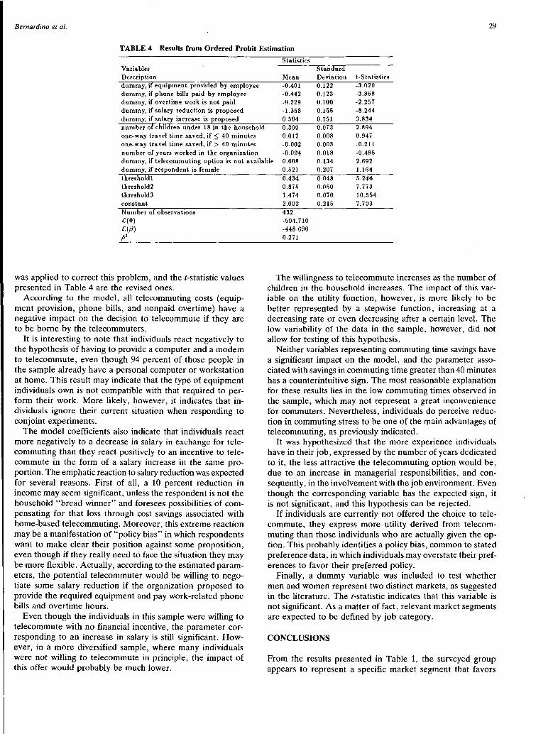
Bernardino et al. 29

TABLE 4 Results from Ordered Probit Estimation

Variables Description dummy, if equipment provided by employee dummy, if phone bills paid by employee dummy, if overtime work is not paid dummy, if salary reduction is proposed dummy, if salary increase is proposed

Statistics

Mean -0.401 -0.442 -0.229 -1.358 0.504

Standard Deviation t-Statistics 0.122 -3.020 0.123 -3.868 0.100 -2.257 0.155 -8.244 0.151 3.834

number of children under 18 in the household one-way travel time saved, if::; 40 minutes one-way travel time saved, if> 40 minutes number of years worked in the organization dummy, if telecommuting option is not available dummy, if respondent is female

0.309 0.012 -0.002 -0.094 0.608 0.521

0.073 0.008 0.003 0.018 0.134 0.207

2.894 0.947 -0.211 -0.485 2.692 1.164

threshold! threshold2 threshold3 constant Number of observations C(O) C(,13) p2

was applied to correct this problem, and the t-statistic values presented in Table 4 are the revised ones.

According to the model, all telecommuting costs (equip­ment provision, phone bills, and nonpaid overtime) have a negative impact on the decision to telecommute if they are to be borne by the telecommuters.

It is interesting to note that individuals react negatively to the hypothesis of having to provide a computer and a modem to telecommute, even though 94 percent of those people in the sample already have a personal computer or workstation at home. This result may indicate that the type of equipment individuals own is not compatible with that required to per­form their work. More likely, however, it indicates that in­dividuals ignore their current situation when responding to conjoint experiments.

The model coefficients also indicate that individuals react more negatively to a decrease in salary in exchange for tele­commuting than they react positively to an incentive to tele­commute in the form of a salary increase in the same pro­portion. The emphatic reaction to salary reduction was expected for several reasons. First of all, a 10 percent reduction in income may seem significant, unless the respondent is not the household "bread winner" and foresees possibilities of com­pensating for that loss through cost savings associated with home-=based telecommuting. Moreover, this extreme reaction may be a manifestation of "policy bias" in which respondents want to make clear their position against some proposition, even though if they really need to face the situation they may be more flexible. Actually, according to the estimated param­eters, the potential telecommuter would be willing to nego­tiate some salary reduction if the organization proposed to provide the required equipment and pay work-related phone bills and overtime hours.

Even though the individuals in this sample were willing to telecommute with no financial incentive, the parameter cor­responding to an increase in salary is still significant. How­ever, in a more diversified sample, where many individuals were not willing to telecommute in principle, the impact of this offer would probably be much lower.

0.434 0.875 1.474 2.002 432 -594.710 -448.690 0.271

0.048 0.050 0.070 0.215

5.2413 7.773 10.554 7.793

The willingness to telecommute increases as the number of children in the household increases. The impact of this var­iable on the utility function, however, is more likely to be better represented by a stepwise function, increasing at a decreasing rate or even decreasing after a certain level. The low variability of the data in the sample, however, did not allow for testing of this hypothesis.

Neither variables representing commuting time savings have a significant impact on the model, and the parameter asso­ciated with savings in commuting time greater than 40 minutes has a counterintuitive sign. The most reasonable explanation for these results lies in the low commuting times observed in the sample, which may not represent a great inconvenience for commuters. Nevertheless, individuals do perceive reduc­tion in commuting stress to be one of the main advantages of telecommuting, as previously indicated.

It was hypothesized that the _more experience individuals have in their job, expressed by the number of years dedicated to it, the less attractive the telecommuting option would be, due to an increase in managerial responsibilities, and con­sequently, in the involvement with the job environment. Even though the corresponding variable has the expected sign, it is not significant, and this hypothesis can be rejected.

If individuals are currently not offered the choice to tele­commute, they express more utility derived from telecom­muting than those individuals who are actually given the op­tion. This probably identifies a policy bias, common to stated preference data, in which individuals may overstate their pref­erences to favor their preferred policy.

Finally, a dummy variable was included to test whether men and women represent two distinct markets, as suggested in the literature. The t-statistic indicates that this variable is not significant. As a matter of fact, relevant market segments are expected to be defined by job category.

CONCLUSIONS

From the results presented in Table 1, the surveyed group appears to represent a specific market segment that favors

30

telecommuting, mainly for its nonmonetary potential benefits. Also, according to Table 2, the main constraint this group faces to adopt telecommuting is merely cultural. At first glance, these observations appear to indicate that these individuals would definitely adopt telecommuting if the option were available.

Nevertheless, the results in Table 4 show that the willing­ness to telecommute is not merely a function of individuals' characteristics and general attitudes toward telecommuting, but also of the characteristics of the working arrangement proposed.

This pilot study demonstrated that even though socioeco­nomic and attitudinal characteristics may be important in in­dividuals' decisions to adopt telecommuting, they do not de­termine adoption because some trade-offs are made in considering the attributes of the proposed arrangement. The relevance of this finding lies in the fact that the organization has the possibility of making a telecommuting program more or less attractive to its employees, according to its own interests.

Due to difficulties in collecting data, the model was re­stricted to stated preferences, presenting validity problems. Therefore, even though it is useful to demonstrate the exist­ence of trade-offs in the decision, the model would probably lead to imprecise forecasts. To improve the external validity of this model, some revealed preference data should be ob­tained to allow for a jointly estimated model [Morikawa (19)].

Moreover, the surveyed sample represents a specific stra­tum and does not represent the population as a whole. To obtain a broader picture of the attractiveness of telecom­muting, a more diversified sample needs to be collected.

ACKNOWLEDGMENTS

The research reported in this paper was sponsored by the International Energy Policy Research Grants, administered by the Massachusetts Institute of Technology (MIT) Center for International Studies. This paper has benefitted from dis­cussions with David Bernstein of the Center for Transpor­tation Studies at MIT.

REFERENCES

1. Olson, M. H. Remote Office Work: Changing Work Patterns in Spaced Time. Communications of the ACM, Vol. 26, No. 3, 1983, pp. 182-187.

TRANSPORTATION RESEARCH RECORD 1413

2. Olson, M. H., and S. B. Primps. Working at Home with Com­puters: Work and Nonwork Issues. Journal of Social Issues, Vol. 40, No. 3, 1984, pp. 97-112.

3. Pratt, J. H. Home Teleworking: A Study of its Pioneers. Tech­nological Forecasting and Social Change, Vol. 25, 1984, pp. 1-14.

4. Kraut, R. E., and P. Grambsch. Prophecy by Analogy: Potential Causes for and Consequences of Electronic Homework. Bell Communications Research, Morristown, N.J., 1985.

5. Bailyn, L. Toward the Perfect Workplace? Communications of the ACM, Vol. 32, No. 4, 1989, pp. 460-471.

6. Christensen, K. The New Era of Home-Based Work: Directions and Policies. Westview Press, Boulder, Colo., 1988.

7. Olson, M. H. Work at Home for Computer Professionals: Cur­rent Attitudes and Future Prospects. ACM Transactions on Office Information Systems, Vol. 7, No. 4, 1989, pp. 317-338.

8. Vitalari, N., A. Venkatesh, and K. Gronhaug. Computing in the Home: Shifts in the Time Allocation Patterns of Households. Communications of the ACM, Vol. 28, No. 5, 1985, pp. 512-522.

9. Kraut, R. E. Predicting the Use of Technology: The Case of Telework. Bell Communications Research, Morristown, N.J., 1985.

10. Spinks, W. A. Satellite and Resort Offices in Japan. Transpor­tation, Vol. 18, No. 4, 1991, pp. 343-364.

11. Salomon, I. Telecommunications and Travel Relationships: A Review. Transportation Research A, Vol. 20A, No. 3, 1986, pp. 223-238.

12. Nilles, J. M. Traffic Reduction by Telecommuting: A Status Re­view and Selected Bibliography. Transportation Research A, Vol. 22A, No. 4, 1989, pp. 301-317.

13. Mokhtarian, P. L. Telecommuting and Travel: State of the Prac­tice, State of the Art. Transportation, Vol. 18, No. 4, 1991, pp. 319-342.

14. Pendyala, R. M., K. G. Goulias, and R. Kitamura. Impact of Telecommuting on Spatial and Temporal Patterns of Household Travel. Transportation, Vol. 18, No. 4, 1991, pp. 383-410.

15. Hamer, R., E. Kroes, and H. Van Ooststroom. Teleworking in the Netherlands: An Evaluation of Changes in Travel Behaviour. Transportation, Vol. 18, No. 4, 1991, pp. 365-382.

16. Nilles, J. M. Telecommuting and Urban Sprawl: Mitigator or Inciter? Transportation, Vol. 18, No. 4, 1991, pp. 411-432.

17. McKelvey, R. D., and W. Zavoina. A Statistical Model for the Analysis of Ordinal Level Dependent Variables. Journal of Math­ematical Sociology, Vol. 4, 1985, pp. 103-120.

18. Miller, R. G. The Jackknife-A Review. Biometrika, Vol. 61, No. 1, 1974.

19. Morikawa, T. Incorporating Stated Preference Data in Travel De­mand Analysis. Ph.D. dissertation. Massachusetts Institute of Technology, Cambridge, 1989.

Publication of this paper sponsored by Committee on Traveler Be­havior and Values.

TRANSPORTATION RESEARCH RECORD 1413 31

Employee Attitudes and Stated Preferences Toward Telecommuting: An Exploratory Analysis

HANI S. MAHMASSANI, ]IN-Ru YEN, ROBERT HERMAN, AND

MARK A. SULLIVAN

The potential effectiveness of telecommuting as a demand man­agement strategy depends on the extent to which it is adopted by firms and accepted by employees. To gain insight into the factors likely to influence the adoption process, a survey of em­ployees was conducted in three Texas cities: Austin, Dallas, and Houston. In this paper the survey results, focusing on the attitudes toward telecommuting held by employees who presently do not telecommute as well as on their stated preferences toward dif­ferent telecommuting options are analyzed. Individual and job­related characteristics likely to influence employee participation in telecommuting programs are identified. The results suggest that successful programs are likely to require some job redesign and means of fair performance evaluation. In addition, success appears to depend on the economic arrangements involved, as most employees seem reluctant to trade income for the flexibility afforded by working from home.

The concept of the electronic homeworker was proposed in 1957 automation literature. It was not until the 1970s, how­ever, that this idea first received public attention, motivated primarily by the energy crisis (J). The term "telecommuting" was initially coined by Nilles and defined as "the partial or total substitution of telecommunications for the daily work trip" (2,3). Telecommuters were first considered as full-time homeworkers. It is now recognized that telecommuting need not to be full time and that working from home is not the only possible type of telecommuting (4). Fqr instance, Nilles defines four types of telecommuting: home based, satellite centers, local centers, and neighborho~d centers (3).

Telecommuting received its second round of public atten­tion in the 1980s. With increasing concern over urban traffic congestion and air quality, telecommuting has been proposed as one element of a broader array of measures aimed at re­ducing work trips and engine emissions in peak hours. In addition, it is advocated as an opportunity for parents with young children or workers with disabilities to participate more fully in the labor force (5 ,6). Furthermore, some managers believe that a properly designed telecommuting program may enhance their company's image as providing a good work environment, thereby improving their ability to recruit qual­ified employees (7). Other advantages of telecommuting are also mentioned in the literature (7-9). For particip~ting em­ployees, the major advantages include (a) less travel time and cost, (b) fewer distractions during work hours, ( c) more sched-

Department of Civil Engineering, University of Texas at Austin, Austin, Tex. 78712.

uling flexibility to meet family commitments, and ( d) greater opportunity to participate in community activities. For the

. companies, the major purported advantages include (a) lower overhead costs for offices, (b) less turnover, (c) higher em­ployee productivity, and ( d) better morale of employees who are telecommuters.

Several possible disadvantages are also identified (7-9). For employees, these include (a) less opportunity for social interaction with coworkers, (b) fewer opportunities for on­the-job learning from senior workers, (c) possibly lower salary under some scenarios, and ( d) fewer opportunities for pro­motion. For companies, the major possible disadvantages in­clude (a) potentially high initial investment, (b) difficulty of performance measurement, (c) resistance from management, (d) resistance from unions, and (e) less data security. Also, some researchers have indicated that telecommuting should be viewed not only as a transportation or management issue, but also as a psychological and sociological issue because it affects the life styles of both the employees and members of their households (9 ,JO).

An essential element in determining the potential impacts of telecommuting is the extent to which it is adopted by firms and their employees. Limited information is available on the adoption process by employees and employers, and most of it is anecdotal or speculative in nature. The objective of the present study is to investigate this process. For this purpose, a survey of firms has been conducted in three Texas cities: Austin, Houston, and Dallas.

According to Fishbein and Ajzen's (11) general attitude­behavior model, behavior is affected by intentions that are in turn influenced by attitudes. Within this framework, Samu­elson and Biek (12) found that individuals' actual energy con­servation behavior is related to their attitudes toward energy use. In the absence of a large base of established telecom­muters, prevailing attitudes toward telecommuting can pro­vide useful insights into the factors that affect a person's like­lihood to adopt telecommuting.

. This study focuses on employees' attitudes and stated pref­erences toward home-based telecommuting, also referred to as "work from home." It presents an exploratory analysis of the data obtained from the telecommuting survey conducted in Austin, Houston, and Dallas, Texas. After describing the survey, the general characteristics of the respondents are sum­mari~ed. Then, the responses to the attitudinal questions are analyzed, including a confirmatory factor analysis to validate

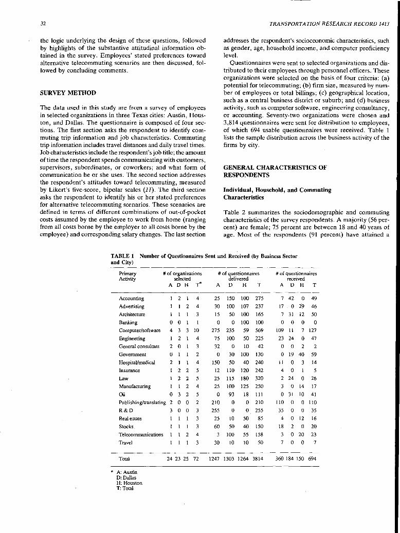
32

the logic underlying the design of these questions, followed by highlights of the substantive attitudinal information ob­tained in the survey. Employees' stated preferences toward alternative telecommuting scenarios are then discussed, fol­lowed by concluding comments.

SURVEY METHOD

The data used in this study are from a survey of employees in selected organizations in three Texas cities: Austin, Hous­ton, and Dallas. The questionnaire is composed of four sec­tions. The first section asks the respondent to identify com­muting trip information and job characteristics. Commuting trip information includes travel distances and daily travel times. Job characteristics include the respondent's job title; the amount of time the respondent spends communicating with customers, supervisors, subordinates, or coworkers; and what form of communication he or she uses. The second section addresses the respondent's attitudes toward telecommuting, measured by Likert's five-score, bipolar scales (JJ). The third section asks the respondent to identify his or her stated preferences for alternative telecommuting scenarios. These scenarios are defined in terms of different combinations of out-of-pocket costs assumed by the employee to work from home (ranging from all costs borne by the employer to all costs borne by the employee) and corresponding salary changes. The last section

TRANSPORTATION RESEARCH RECORD 1413

addresses the respondent's socioeconomic characteristics, such as gender, age, household income, and computer proficiency level.

Questionnaires were sent to selected organizations and dis­tributed to their employees through personnel officers. These organizations were selected on the basis of four criteria: (a) potential for telecommuting; (b) firm size, measured by num­ber of employees or total billings; (c) geographical location, such as a central business district or suburb; and (d) business activity, such as computer software, engineering consultancy, or accounting. Seventy-two organizations were chosen and 3,814 questionnaires were sent for distribution to employees, of which 694 usable questionnaires were received. Table 1 lists the sample distribution across the business activity of the firms by city.

GENERAL CHARACTERISTICS OF RESPONDENTS

Individual, Household, and Commuting Characteristics

Table 2 summarizes the sociodemographic and commuting characteristics of the survey respondents. A majority (56 per­cent) are female; 75 percent are between 18 and 40 years of age. Most of the respondents (91 percent) have attained a

TABLE 1 Number of Questionnaires Sent and Received (by Business Sector and City)

Primary Activity

# of organizations selected

A DH T*

Accounting 2 1 4

Advertising 1 2 4

Architecture 1 1 3 Banking 0 0 1 1 Computer/software 4 3 3 10 Engineering 1 2 4

General consultant 2 0 3 Government 0 2 Hospital/medical 2 1 4

Insurance 2 2 5

Law 2 2 5

Manufacturing 1 1 2 4

Oil 0 3 2 5

Publishing/translating 2 0 0 2 R&D 3 0 0 3 Real estate 3 Stocks, 1 3 Telecommunications 2 4

Travel 3

Total 24 23 25 72

* A: Austin D:Dallas H: Houston T: Total.

# of questionnaires delivered

A D H T

25 150 100 275

30 100 107 237

15 50 100 165 0 0 100 100

275 235 59 569 75 100 50 225

32 0 10 42

0 30 100 130 150 50 40 240

12 110 120 242

25 115 180 320

25 100 125 250

0 93 18 111

210 0 0 210

255 0 0 255

25 10 50 85

60 50 40 150

3 100 55 158

30 10 10 50

1247 1303 1264 3814

# of questionnaires received

A D H T

7 42 0 49 17 . 0 29 46 7 31 12 50 0 0 0 0

109 11 7 127

23 24 0 47

0 0 2 2 0 19 40 59

11 0 3 14 4 0 1 5

2 24 0 26 3 0 14 17 0 31 10 41

110 0 0 110 35 0 0 35 4 0 12 16

18 2 0 20 3 0 20 23 7 0 0 7

360 184 150 694

TABLE 2 Individual and Household Characteristics

Characteristics

Gender

Age

Educational level

Categories

Male Female

Under 18 18-30 31-40 41-50 51-60 above 60

Finished high school

Relatiye frequency (%)

44.3 55.7

0.0 35.6 39.8 17.4 5.5 1.7

4.2 Some college or university Finished college or university Master

25.0 48.6 16.3

Household income/year

Number of telephone lines at home

With FAX at home

Subscription to electronic home-shopping

Ph.D. Other

Less than 25,000 25,000-50,000 50,000-75,000 More than 75,000

0 1 2 3 4

Yes No

Yes No

Number of personal computers 0 at home 1

2 3

Proficiency level in word processing

Proficiency level in spreadsheets

Proficiency level in data processing packages

Proficiency level in computer programming

Proficiency level in computer graphics packages

Distance from home to the workplace (miles)*

AM travel time from home to the workplace (minutes)*

PM travel time from the workplace to home (minutes)*

AM stops on the way from home to the workplace, per week*

PM stops on the way from the workplace to home, per week*

high medium low non-existent

high medium low non-existent

high medium low non-existent

high medium· low non-existent

high medium low non-existent

mean standard deviation

mean standard deviation

mean standard deviation

mean standard deviation

mean standard deviation

* : Numbers in these items are not relative frequencies.

1.4 4.5

12.7 44.0 28.9 14.3

2.0 85.3 11.5

1.0 0.1

1.9 98.1

6.5 93.5

53.I 42.4

3.5 1.0

40.3 35.3 13.0 11.4

22.0 28.0 22.0 28.0

10.0 20.2 25.4 44.4

13.7 8.2

21.2 56.8

14.5 18.8 24.9 41.9

14.0 10.8

26.5 15.8

28.8 17.0

2.0 3.0

3.8 3.5

34

high education level, with 66 percent having completed col­lege or university and 18 percent having attained a master's or doctorate degree. The household income is approximately normally distributed, with the mode in the range of $25,000 to $50,000/year.

Employees were also asked about the number of telephone lines, facsimile equipment, and personal computer availability at home, because such equipment may be of use in telecom­muting. Only 13 percent of the respondents have more than one telephone line at home. The penetration of home facsim­ile machines is still limited, with 98 percent of the respondents not owning such equipment. Personal computers are more prevalent, with 47 percent of respondents having at least one personal computer at home, and 5 percent reporting at least two units. However, only 7 percent use electronic data bases or computer-based teleshopping.

To the extent that workers with good computer skills have been identified as a likely target group for telecommuting, the survey asked about proficiency levels in different computer­related skills. Among the respondents, 76 percent have at least a medium level proficiency in the use of work processing

TABLE 3 Job Titles and Job Categories

Job category Job title

TRANSPORTATION RESEARCH RECORD 1413

packages, 50 percent for spreadsheets, 30 percent for data processing packages, 22 percent for computer language pro­gramming, and 33 percent for computer graphics packages. Overall, 84 percent of the respondents have at least one com­puter skill at medium or high level.

Commuting information in Table 2 indicates that the re­spondents on average encounter longer travel time and make more stops in the afternoon trip than in the morning trip. However, considerable variability in these quantities is pres­ent across the respondents.

Job Characteristics

Thirty-four job titles were mentioned by the respondents, vary­ing from president to engineer to clerk. These job titles are grouped into 12 categories, (see Table 3) based on three ·cri­teria: power in the organizational strategic decision process, schedule flexibility, and suitability for telecommuting. Cate­gories 1 (president/vice president) and 2 (manager/supervisor) have more power in the decision-making process than others.

Freq. Pere. Freq. Pere. (*) (*) (**) (**)

1. President I vice president President I vice president 10 1.5 10 1.5

2. Manager I supervisor Director I administrator 27 3.9 108 15.7 Senior associate 12 1.7 Supervisor I manager 54 7.9 Technical manager 15 2.2

3. Writer I editor Writer 7 1.0 60 8.7 Editor 47 6.9 Photo research 6 0.9

4. Accountant I attorney Accountant I tax consultant 59 8.6 72 10.5 Attorney 13 1.9

5. Agent Broker 3 0.4 15 2.2 Real estate agent 7 1.0 Travel agent 5 0.7

6. Computer programmer Computer programmer 57 8.3 57 8.3

7. Data processing Data processing 10 1.5 14 2.0 Book keeper 2 0.3 Typist 2 0.3

8. Engineer I researcher Consultant 12 1.7 122 17.8 Engineer I Architect 92 13.4 R & D scientist 18 2.6

9. Field worker Clerk I general labor 25 3.6 39 5.7 Registered nurse 7 1.0 Teamster 1 0.1 Plumber I mechanic I carpenter 6 0.9

10. Receptionist I secretary Receptionist 3 0.4 49 7 .1 Secretary 46 6.7

11. Coach I trainer Coach 1 0.1 8 1.2 School I community liaison 4 0.6 Training specialist 3 0.4

12. General employee Administration assistant 37 5.4 132 19.2 Sales I marketing representative 47 6.9 General government employee 1 0.1 Customer I support analyst 36 5.2 Production coordinator 11 1.6

Total 686 100.0

* : for Job title

**:for Job category

Mahmassani et al.

Categories 3 (writer/editor), 4 (accountant/attorney), and 5 (agent) are assumed to have more schedule flexibility. Cat­egories 6 (computer programmer), 7 (data processing), and 8 (engineer/researcher) are considered to have the most po­tential for telecommuting. Categories 9 (field worker) and 10 (receptionist/secretary) probably have the least potential for telecommuting. According to Table 3, general employee (19 percent), engineer/researcher (18 percent), and manager/ supervisor (16 percent) are the largest three job categories in the sample.

EMPLOYEE ATTITUDES TOWARD TELECOMMUTING

This section discusses the responses to the questions intended to identify the employees' attitudes toward telecommuting. First, the logic underlying the design of the attitudinal ques­tions is validated by a confirmatory factor analysis of the responses. An exploratory analysis and discussion of the re­sponses is presented next, followed by statistical tests aimed at identifying the principal characteristics of the employees and their jobs that influence their attitudes.

Question Design Logic and Confirmatory Factor Analysis

The 18 attitudinal questions used in this survey (see Table 4) in connection with the response of each question were de­signed to measure the following seven general attitudes:

• Attitude toward and/or perception of transportation sys­tem performance (Questions 1, 2, and 3),

•Importance of working in the office (Questions 7, 8, and 9),

•Importance of social interaction with coworkers (Ques­tions 10 and 11),

•Job suitability for telecommuting (Questions 12 through 15),

• Expectation of the effect of telecommuting on job perfor­mance (Questions 16 and 18),

•Expectation of the effect of telecommuting on one's fam­ily (Questions 4 and 17), and

• Preference toward working independently (Questions 5 and 6).

A principal component analysis (PCA) and a confirmatory factor analysis (CF A) were performed to confirm whether the variation of the responses to the 18 questions could be ex­plained by the underly~ng seven attitudes. The measured var­iables in the factor analysis models correspond to the re­sponses to these questions, respectively, with the exception of Variable 1. The number 6 was subtracted from all responses to Question 1 to keep Variables 1, 2, and 3 consistent. The number of factors is specified to be seven in the PCA model. The rotated factor pattern in Table 5, obtained using the promax rotation procedure to address the correlations among factors (13), supports the above design rationale quite well. The cumulative amounts of variation explained to the factors are 2.3, 4.4, 5.8, 8.4, 10.1, 11.4, and 12.6, respectively, in-

35

dicating that these seven factors together explain 70 percent of the measured variation (12.7/18 = 0.7).

In the confirmatory factor analysis, performed using the SAS CALIS procedure (14), the factor pattern is specified as above, with assumed correlations among factors. The esti­mates of the loadings of variables, reported in Table 6 along with the corresponding t-values, indicate that all are signifi­cantly different from zero at the 0.01 level. In addition, 10 variables load on the specified factors with values greater than 0.60, usually considered a high loading, while only 1 variable has a loading less than 0.30, which is considered a low loading. Statistics such as the goodness-of-fit index (GFI = 0.90) and adjusted GFI (0.86) indicate that the model fits the observed data very well. An inspection of the residual correlation ma­trix also shows that the estimated factor loadings predict the correlation matrix fairly well.

Table 7 shows the estimated correlation coefficients be­tween factors. While all terms are significant at the 0.01 level, most of the coefficients are less than 0.5 or greater than -0.5, indicating that, in general, the correlations among factors are not high. The two highest correlations exist between factors 6 and 7 (0.90) and factors 6 and 5 (0.83). That is, there appear to be strong positive correlations between an employee's ex­pectation of the effects of telecommuting on the family and his or her preference for working independently as well as his

. or her expectation of the effect of telecommuting on job performarice.

Discussion of Responses

The responses to the individual questions are shown in Table 4. With regard to the first attitude pertaining to the trans­portation system, half of the commuters in the sample do not find commuting to work stressful (Question 1). Thirty-three percent think that the traffic is smooth from home to the workplace, although 41 percent think it is congested. On the other hand, 24 percent of the respondents believe the traffic is smooth on the way back home, although 54 percent believe it is congested, confirming the finding in other studies that commuters experience a longer evening commute than in the morning (15).

With respect to the importance of working in the office, 60 percent of the respondents believe that it is essential to their work to have frequent input from their supervisor or co­workers, while less than 20 percent believe it is not. In re­sponse to Question 8, 44 percent believe it is important to attend short-notice meetings during the work hours; 36 per­cent believe it is unimportant'. Seventy percent of the respon­dents believe it is important to have immediate access to information or references available only at the office; only 14 percent believe it is unimportant.

The responses to the questions that address the importance of social interaction with coworkers indicate that 50 percent of the respondents believe it is important to have social in­teractions with their coworkers at work (Question 10), but only 13 percent feel it is important outside of work' (Ques­tion 11).

With regard to the job's suitability for telecommuting, only 21 percent of the respondents believe their jobs are suitable for working from home everyday. This number increases to

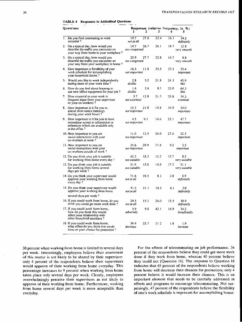
36 TRANSPORTATION RESEARCH RECORD 1413

TABLE 4 Responses to Attitudinal Questions

Questions

1. Do you find commuting to work stressful?

2. On a typical day, how would you describe the traffic you encounter on your way from home to your workplace ?

3. On a typical day, how would you describe the traffic you encounter on your way from your workplace to home ?

4. How important is flexibility of your work schedule for accomplishing your household duties ?

5. Would you like to work independently during more of your work time ?

6. How do you feel about learning to use new office equipment for your job ?

7. How essential to your work is frequent input from your supervisor or your co-workers ?

8. How important is it for you to . attend short-notice meetings during your work hours?

9. How important is it for you to have immediate access to information or references which are available only at the office ?

10. How· important to you are social interactions with your co-workers at work ?

11. How important to you are social interactions with your co-workers outside of work?

12. Do you think your job is suitable for working from home every day ?

13. Do you think your job is suitable for working from home several days per week?

14. Do you think your supervisor would approve your working from home every day?

15. Do you think your supervisor would approve your working from home

several days per week ?

16. If you could work from home, do you think you could get more work done ?

17. If you could work from home, how do you think this would affect your relationship with other household members ?

18. If you could work from home, what effect do you think this would have on your chance for promotion ?

38 percent when working from home is limited to several days per week. Interestingly, employees believe their assessment of this matter is not likely to be shared by their supervisor: only 4 percent of the respondents believe their supervisors would approve of their working from home everyday. This percentage increases to 9 percent when working from home takes place only several days per week. Clearly, employees overwhelmingly perceive their supervisors as not likely to approve of their working from home. Furthermore, working from home several days per week is more acceptable than everyday.

Responses (relative frequency, in %) 1 2 3 4 5

19.7 27.6 22.4 16. l 14.2 not at all definitely

14.7 26.7 26.l 19.7 12.8 too congested very smooth

25.9 27.7 22.8 14.7 8.8 too congested very smooth

16.3 11.8 25.5 23.1 23.4 not important important

2.8 5.2 21.8 24.3 45.9 dislike like

1.4 2.6 8.7 23.0 64.3 dislike like

5.7 12.9 21.3 25.8 34.3 not essential essential

15.3 21.0 19.8 19.9 24.0 not important important

4.5 9.1 16.6 22.1 47.7 not important important

11.0 12.9 26.0 27.6 22.5 not important important

35.6 29.9 21.8 9.2 3.5 not important important

45.3 18.3 15.2 12.7 8.5 not suitable very suitable

31.9 15.0 14.9 17.2 21.1 not suitable very suitable

71.6 16.5 8.3 2.8 0.9 not at all definitely

51.5 21.1 18.2 6.1 3.0 not at all definitely

24.5 15.1 26.0 15.5 18.9 not at all definitely

5.9 9.0 42.l 18.8 24.2 adversely beneficially

39.4 25.7 31.2 1.8 1.9 decrease increase

For the effects of telecommuting on job performance, 34 percent of the respondents believe they could get more work done if they work from home, whereas 40 percent believe they could not (Question 16). The response to Question 18 indicates that 65 percent of the respondents believe working from home will decrease their chances for promotion; only 4 percent believe it would increase their chances. This is an important element that needs to be carefully addressed in efforts and programs to encourage telecommuting. Not sur­prisingly, 47 percent of the respondents believe the flexibility of one's work schedule is important for accomplishing house-

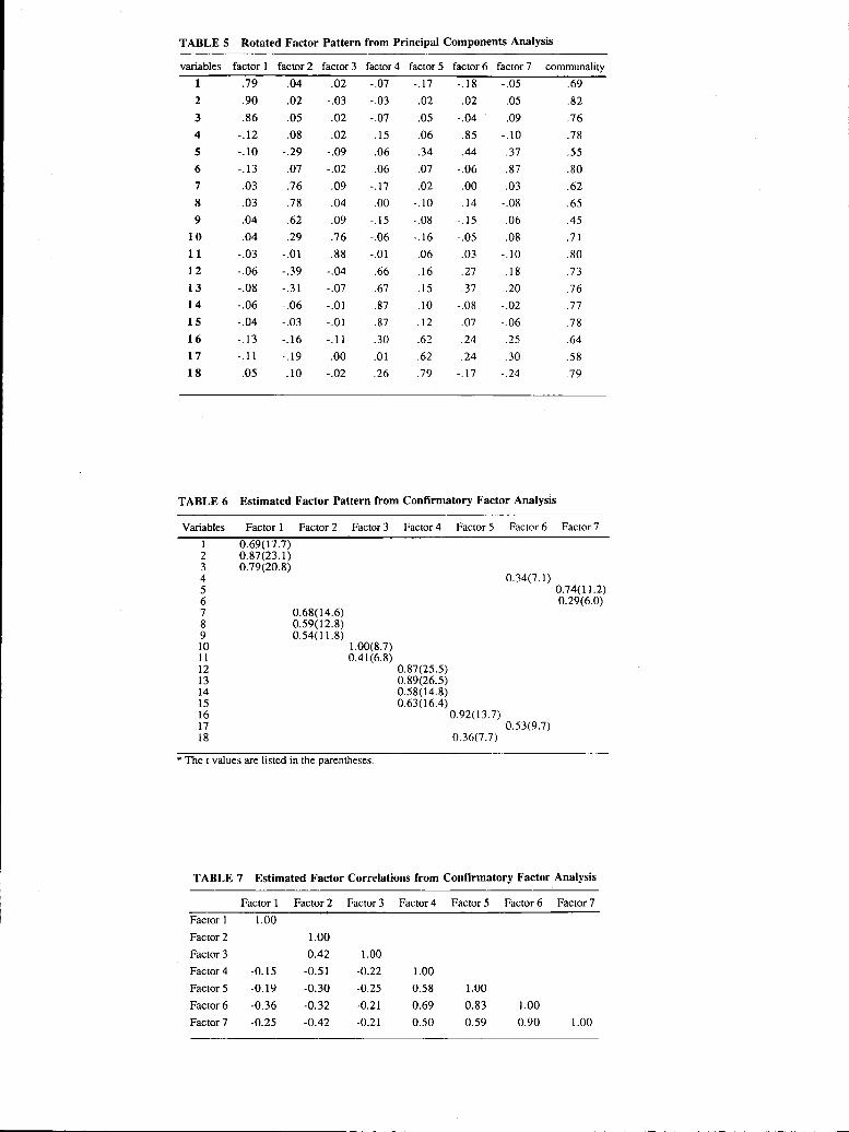
TABLE 5 Rotated Factor Pattern from Principal Components Analysis

variables factor 1 factor 2 factor 3 factor 4 factor 5 factor 6 factor 7 communality

1 .79 .04 .02 -.07 -.17 -.18 -.05 .69

2 .90 .02 -.03 -.03 -.02 .02 -.05 .82

3 .86 .05 .02 -.07 .05 -.04 -.09 .76

4 -.12 .08 .02 .15 .06 .85 -.10 .78

5 -.10 -.29 -.09 .06 .34 .44 .37 .55

6 -.13 .07 -.02 .06 .07 -.06 .87 .80

7 .03 .76 .09 -.17 .02 .00 .03 .62

8 .03 .78 .04 .00 -.10 .14 -.08 .65

9 .04 .62 .09 -.15 -.08 -.15 .06 .45

10 .04 .29 .76 -.06 -.16 -.05 .08 .71

11 -.03 -.01 .88 -.01 .06 .03 -.10 .80

12 -.06 -.39 -.04 .66 .16 .27 .18 .73

13 -.08 -.31 -.07 .67 .15 .37 .20 .76

14 -.06 -.06 -.01 .87 .10 -.08 -.02 .77

15 -.04 -.03 -.01 .87 .12 .07 -.06 .78

16 -.13 -.16 -.11 .30 .62 .24 .25 .64

17 -.11 -.19 .00 .01 .62 .24 .30 .58

18 .05 .10 -.02 .26 .79 -.17 -.24 .79

TABLE 6 Estimated Factor Pattern from Confirmatory Factor Analysis

Variables Factor 1 Factor 2 Factor 3 Factor 4 Factor 5 Factor 6 Factor 7

1 0.69(17.7) 2 0.87(23.1) 3 0.79(20.8) 4 0.34(7.1) 5 0.74(11.2) 6 0.29(6.0) 7 0.68(14.6) 8 0.59(12.8) 9 0.54(11.8) 10 1.00(8.7) 11 0.41 (6.8) 12 0.87(25.5) 13 0.89(26.5) 14 0.58(14.8) 15 0.63(16.4) 16 0.92(13.7) 17 0.53(9.7) 18 0.36(7.7)

* The t values are listed in the parentheses.

TABLE 7 Estimated Factor Correlations from Confirmatory Factor Analysis

Factor 1 Factor 2 Factor 3 Factor4 Factor 5 Factor 6 Factor?

Factor 1 1.00

Factor2 1.00

Factor 3 0.42 1.00

Factor4 -0.15 -0.51 -0.22 1.00

Factor 5 -0.19 -0.30 -0.25 0.58 1.00

Factor 6 -0.36 -0.32 -0.21 0.69 0.83 1.00

Factor? -0.25 -0.42 -0.21 0.50 0.59 0.90 1.00

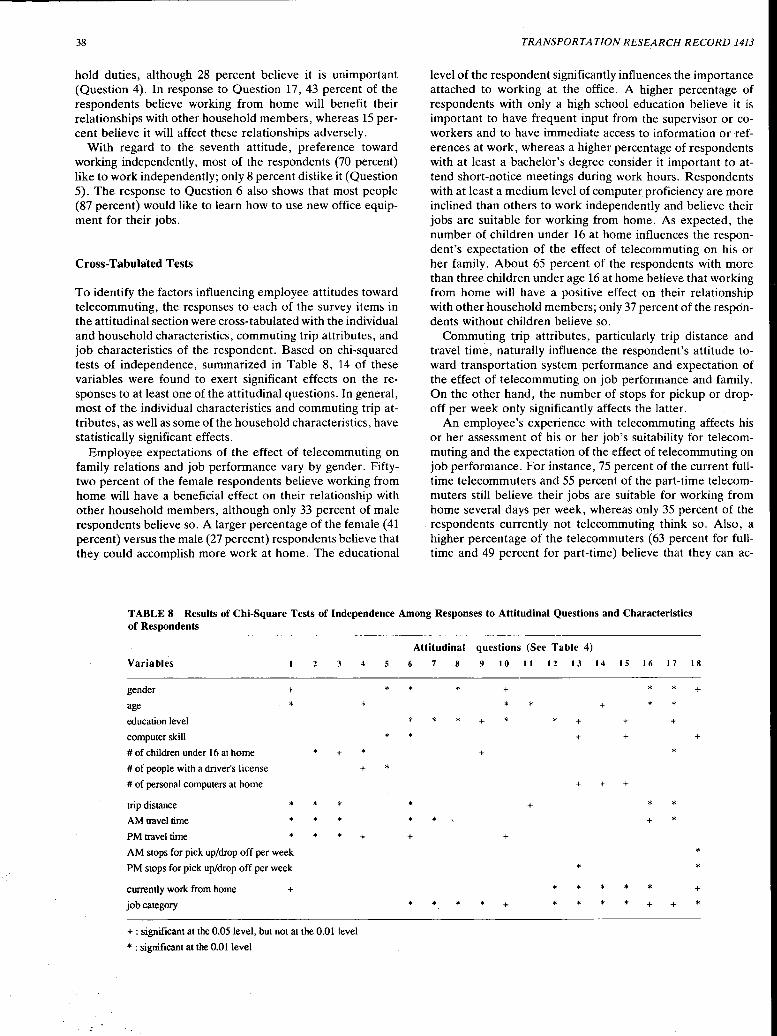
38

hold duties, although 28 percent believe it is unimportant (Question 4). In response to Question 17, 43 percent of the respondents believe working from home will benefit their relationships with other household members, whereas 15 per­cent believe it will affect these relationships adversely.

With regard to the seventh attitude, preference toward working independently, most of the respondents (70 percent) like to work independently; only 8 percent dislike it (Question 5). The response to Question 6 also shows that most people (87 percent) would like to learn how to use new office equip­ment for their jobs.

Cross-Tabulated Tests

To identify the factors influencing employee attitudes toward telecommuting, the responses to each of the survey items in the attitudinal section were cross-tabulated with the individual and household characteristics, commuting trip attributes, and job characteristics of the respondent. Based on chi-squared tests of independence, summarized in Table 8, 14 of these variables were found to exert significant effects on the re­sponses to at least one of the attitudinal questions. In general, most of the individual characteristics and commuting trip at­tributes, as well as some of the household characteristics, have statistically significant effects.

Employee expectations of the effect of telecommuting on family relations and job performance vary by gender. Fifty­two percent of the female respondents believe working from home will have a beneficial effect on their relationship with other household members, although only 33 percent of male respondents believe so. A larger percentage of the female (41 percent) versus the male (27 percent) respondents believe that they could accomplish more work at home. The educational

TRANSPORTATION RESEARCH RECORD 1413

level of the respondent significantly influences the importance attached to working at the office. A higher percentage of respondents with only a high school education believe it is important to have frequent input from the supervisor or co­workers and to have immediate access to information or ref­erences at work, whereas a higher percentage of respondents with at least a bachelor's degree consider it important to at­tend short-notice meetings during work hours. Respondents with at least a medium level of computer_ proficiency are more inclined than others to work independently and believe their jobs are suitable for working from home. As expected, the number of children under 16 at home influences the respon­dent's expectation of the effect of telecommuting on his or her family. About 65 percent of the respondents with more than three children under age 16 at home believe that working from home will have a positive effect on their relationship with other household members; only 37 percent of the resp6n­dents without children believe so.

Commuting trip attributes, particularly trip distance and travel time, naturally influence the respondent's attitude to­ward transportation system performance and expectation of the effect of telecommuting on job performance and family. On the other hand, the number of stops for pickup or drop­off per week only significantly affects the latter.

An employee's experience with telecommuting affects his or her assessment of his or her job's suitability for telecom­muting and the expectation of the effect of telecommuting on job performance. For instance, 75 percent of the current full­time telecommuters and 55 percent of the part-time telecom­muters still believe their jobs are suitable for working from home several days per week, whereas only 35 percent of the

. respondents currently not telecommuting think so. Also, a higher percentage of the telecommuters ( 63 percent for full­time and 49 percent for part-time) believe that they can ac-

TABLE 8 Results of Chi-Square Tests of Independence Among Responses to Attitudinal Questions and Characteristics of Respondents

Attitudinal questions (See Table 4)

Variables 4 5 7 8 9 10 11 12 13 14 15 16 17 18

gender + * * * + * * +

age * * * + * education level * * + + + +

computer skill * * + + +

#of children under 16 at home * + * + * #of people with a driver's license + * # of personal computers at home + + +

trip distance * * * + * AM travel time * * * * * + * PM travel time * * * + + +

AM stops for pick up/drop off per week * PM stops for pick up/drop off per week * * currently work from home + * * * * * +

job category * * * * + * * * * + + *

+: significant at the 0.05 level, but not at the 0.01 level

* : significant at the 0.01 level

Mahmassani et al.

complish more work by telecommuting, while only 32 percent of nontelecommuters believe so. None of the full-time tele­commuters think telecommuting will increase their chance for promotion, although 17 percent of the part-time telecom­muters and 4 percent of the nontelecommuters think so. Of course, job category also affects the respondent's assessment of his or her job's suitability for telecommuting. In gen­eral, a smaller percentage of respondents within Category 1 (president/vice president), Category 2 (manager/supervisor), and Category 10 (receptionist/secretary) believe their jobs are suitable for working from home. On the other hand, a higher percentage of respondents within Category 3 (writer/editor), Category 5 (agent), Category 6 (computer programmer), and Category 7 (data processing) indicate that their jobs are suit­able for telecommuting.

STATED PREFERENCES FOR TELECOMMUTING ALTERNATIVES

This section discusses the responses to the questions regarding the employees' willingness to participate in different types of telecommuting options. After describing the various options and the responses, an exploratory analysis of some of the underlying factors influencing these responses is presented.

Discussion of Responses

Seven telecommuting program scenarios were defined in terms of who assumes the costs incurred to work from home and corresponding salary changes. Table 9 lists these alternative scenarios and the corresponding responses. For each alter­native scenario, the employee was asked to state a preference in the form of one of the following responses: (a) working

39

from home everyday, (b) working from home several days per week, (c) possibly working from home, and (d) not to work from home. The response option to possibly work from home was unavailable for Scenario 4.

Scenario 4 (salary increases, no cost to employee) was de­signed to dominate all others, as confirmed by the results, with 86.1 percent of the respondents interested in telecom­muting at least several days per week. Scenario 1 reflects the status quo (same salary, no cost to employee). Under this scenario, about 66 percent of the respondents will choose to work from home at least several days per week, with 22 per­cent indicating they do not exclude the possibility. The desire to telecommute is quickly dampened as employees are asked to incur some of the additional costs that may be required. The percentage of willing telecommuters drops to 38 percent if the employee has to pay for an additional phone line (Sce­nario 2), and to 29 percent if a computer must be purchased (Scenario 3). Apparently a 5 percent increase in salary may not be sufficient to compensate for some of these costs (Sce­nario 5), as suggested by the 28 percent categorical refusal to telecommute compared to about 12 percent under the status quo (Scenario 1).

Salary decreases certainly do not encourage telecommuting and appear to be even less tolerated than having to assume some of the costs of telecommuting. Under Scenario 6 (5 percent salary decrease, no additional cost to employee), the percentage of willing telecommuters decreases to 21 percent and further drops to 10 percent if one has to give up 10 percent of his or her salary (Scenario 7).

These results allow us to estimate the percentage of "hard core" telecommuters at no more than 15 percent and those that would not even think of telecommuting also at about 15 percent. This means that the participation of the majority of employees in a telecommuting program will depend on the specifics of the program, particularly its cost implications.

TABLE 9 Responses to Stated Preference for Telecommuting Program Scenarios

Telecommuting and Program Scenario

Responses (relative frequency, in percent)* 1 2 3 4

1. Salary stays the same; employer pays all costs 21.6 44.5 22.0 11.8

2. Salary stays the same; employee incurs cost of a new telephone number 11.9 25.8 33.4 28.9

3. Salary stays the same; employee buys a personal computer 9.2 16.0 31.8 43.0

4. Salary increases 5%; employer pays all costs 34.0 52.1 ** 13.8

5. Salary increases 5%; employee pays part of the costs 16.2 28.2 27.8 27.8

6. Salary decreases 5%; employer pays all costs 7.9 12.8 21.2 58.1

7. Salary decreases 10%; employer pays all costs 5.2 5.0 12.4 77.4

* 1: Would like to work from home everyday. 2: Would like to work from home several days per week. 3: Possibly would like to work from home. 4: Do not want to work from home.

** This scenario only allowed three responses in the questionnaire.

~>

·',

·,· r •'

40

Employees do not appear to value telecommuting sufficiently to take a pay cut for the privilege. Some may be willing to incur a small cost to acquire necessary equipment.

It can also be noted that under all program scenarios, more employees would rather telecommute only a few days per week instead of every day.

Cross-Tabulated Tests

The responses to the alternative telecommuting scenarios were also cross-tabulated with the same variables considered in the attitudinal analysis. The same 14 variables found to signifi­cantly influence employees' attitudes were also found to have effects on their stated preferences toward the various tele­commuting program scenarios. Table 10 summarizes these results.

Consistent with the results of the attitudinal analysis, female respondents express a stronger preference for working from home than do male employees. For example, under the status quo Scenario 1, 73 percent of the female respondents stated that they would like to work from home at least several days per week, but only 58 percent of the responding males ex­pressed such a preference. Again, this reflects the previous findings that more of the female respondents believe working from home will have a beneficial effect on their relationship with other household members and on their work productiv­ity. Another result consistent with the attitudes uncovered earlier is that a larger percentage of respondents with at least medium proficiency in the use of computers would like to work from home. Similarly, respondents who own at least one personal computer at home express a stronger preference for telecommuting. For example, 60 percent of respondents with at least one computer would prefer to work from home under Scenario 5; only 40 percent of those with no home

TRANSPORTATION RESEARCH RECORD 1413

computers would prefer to work from home under the same scenario.

Various household characteristics also affect the employee's preference for telecommuting. Under Scenario 1, 90 percent of the respondents with more than two children under 16 at home would like to work from home, although 63 percent of the respondents without children would like to do so also.

In general, commuting trip attributes do not affect the em­ployee's assessment of his or her job's suitability for telecom­muting. However, these attributes significantly affect the em­ployee's stated preferences for the various telecommuting scenarios. A higher percentage of respondents with longer trip distances or travel time prefer to work from home than others. For example, under Scenario 1, 70 percent of the respondents with morning travel time greater than 19 min (the sample mean plus half of the standard deviation) would like to work from home, compared with 59 percent of the respondents with morning travel less than 9 min (the sample mean minus half of the standard deviation).

Also consistent with the attitudinal results, the employee's prior experience with telecommuting and job category affect his or her preference for telecommuting. A greater percentage of current full-time or part-time telecommuters indicate a preference for telecommuting than those without such ex­perience. A smaller percentage of respondents within the management group (Categories 1 and 2) would like to work from home than those in other job categories. This result is consistent with the attitudinal analysis that found that a smaller fraction of these respondents believe their jobs are suitable for telecommuting. On the other hand, although employees in Categories 9 (field worker) and 10 (receptionist/secretary) had indicated that these jobs are not readily telecommutable, a large percentage of them still indicated that they would like to work from home.

TABLE 10 Results of Chi-Square Tests of Responses to Stated Preference Questions

Stated preference questions

Variables 1 2 3 4 5 6 7

gender * * +

age + * + + +

education level * +

computer skill . * * + +

# of children under 16 at home + * * * #people with a driver's license * * + * #of personal computers at home * * trip distance + * + * AM travel time * + * +

PM travel time * * * +

AM stops for pick up/drop off per week * + + +

PM stops for pick up/drop off per week * * + + +

currently work from home * * + +

job category * + + *

+:significant at the 0.05 level, but not at the 0.01 level

* : significant at the 0.01 level

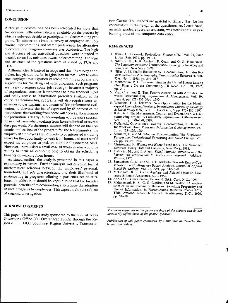
Mahmassani et al.

CONCLUSION

Although telecommuting has been advocated for more than two decades, little information is available on the process by which employees decide to participate in telecommuting pro­grams. To address this issue, a survey of employee attitudes toward telecommuting and stated preferences for alternative telecommuting program scenarios was conducted. The logic and structure of the attitudinal questions were intended to identify seven key attitudes toward telecommuting. The logic and structure of the questions were validated by PCA and CFA.

Although clearly limited in scope and size, the survey none­theless has yielded useful insights into factors likely to influ­ence employee participation in telecommuting programs and suggestions for the design of such programs. Such programs are likely to require some job redesign, because a majority of respondents consider it important to have frequent input and ready access to information presently available at the office. Telecommuting programs will also require some as­surances to participants, and means of fair performance eval­uation, to alleviate the belief expressed by 65 percent of the respondents that working from home will decrease their chances for promotion. Clearly, telecommuting will be more success­ful in most cases when working from home is limited to several days per week. Furthermore, success will depend on the eco­nomic implications of the program for the telecommuter; the majority of employees are not likely to be interested in trading salary for the opportunity to work from home, and most would expect the employer to pick up additional associated costs. However, there exists a small core of workers who would be willing to incur an economic cost to obtain the scheduling benefits of working from home.

As stated earlier, the analysis presented in this paper is exploratory in nature. Further analysis will establish formal mathematical relations between the employees' personal, household, and job ch~racteristics, and their likelihood of participating in programs offering a particular set of attri­butes. In addition, it should be kept in mind that the broader potential benefits of telecommuting also require the adoption of such programs by employers. This aspect is also the subject of ongoing investigation.

ACKNOWLEDGMENTS

This paper is based on a study sponsored by the State of Texas Governor's Office (Oil Overcharge Funds) through the Re­gion 6 U.S. DOT Southwest Region University Transporta-

41

tion Center. The authors are grateful to Hillary Hart for her contribution to the design of the questionnaire. Laura Brod, an undergraduate research assistant, was instrumental in per­forming most of the computer data entry.

REFERENCES

1. Huws, U. Telework: Projections. Futures (UK), Vol. 23, Issue 1, Jan-Feb. 1991, pp. 19-31.

2. Nilles, J. M., F. R. Carlson, P. Gray, and G. G. Hanneman. The Telecommunications-Transportation Tradeoff. John Wiley and Sons, Inc., New York, 1976.

3. Nilles, J. M. Traffic Reduction by Telecommuting: A Status Re­view and Selected Bibliography. Transportation Research A, Vol. 22A, No. 4, 1988, pp. 301-317.

4. Mokhtarian, P.· L. Telecommuting in the United States: Letting Our Fingers Do the Commuting. TR News, No. 158, 1992, pp. 2-7.

5. Yap, C. S., and H. Tng. Factors Associated with Attitudes To­wards Telecommuting. Information & Management, Vol. 19, Issue 4, pp. 227-235, Nov. 1990.

6. Woelders, H. J. Telework: New Opportunities for the Handi­capped Unemployed Workers. International Journal of Sociology & Social Policy (UK), Vol. 10, Issues 4, 5, 6, pp. 176-180, 1990.

7. Katz, A. I. The Management, Control, and Evaluation of a Tele­commuting Project: A Case Study. Information & Management, Vol. 13, pp. 179-190, 1987.

8. Desanctis, G. Attitudes Towards Telecommuting: Implications for Work-At-Home Programs. Information & Management, Vol. 7, pp. 133-139, 1984.

9. Salomon, I., and M. Salomon. Telecommuting: The Employees' Perspective. Technological Forecasting and Social Change, Vol. 25, pp. 15-28, 1984.

10. Christensen, K. Women and Home-Based Work: The Unspoken Contract. Henry Holt and Company, New York, 1988.

11. Fishbein, M., and I. Ajzen. Belief, Attitude, Intention and Be­havior: An Introduction to Theory and Research. Addison­Wesley, 1975.

12. Samuelson, C. D., and M. Biek. Attitudes Towards Energy Con­servation: A Confirmatory Factor Analysis. Journal of Applied Social Psychology, Vol. 21, 1991, pp. 549-568.

13. McDonald, R. P. Factor Analysis and Related Methods. Law­rence Erlbaum Associates, N.J., 1985.

14. SAS/STAT User's Guide, Version 6. SAS, Cary, N.C., 1990. 15. Mahmassani, H. S., C. G. Caplice, and M. Walton. Character­

istics of Urban Commuter Behavior: Switching Propensity and Use of Information. In Transportation Research Record 1285, TRB, National Research Council, Washington, D.C., 1990, pp. 57-69.

The views expressed in this paper are those of the authors and do not necessarily reflect those of the project sponsors.

Publication of this paper sponsored by Committee on Traveler Be­havior and Values.

42 TRANSPORTATION RESEARCH RECORD 1413

Choice Model of Employee Participation in Telecommuting Under a Cost-Neutral Scenario

MARK A. SULLIVAN, HANI S. MAHMASSANI, AND JIN-Ru YEN

A multinomial logit model was constructed of employee partic­ipation in telecommuting using stated preference data extracted from a survey of employees of information-oriented firms in Aus­tin, Dallas, and Houston, Texas. Respondents were given work site alternatives in a scenario in which all telecommuting costs were incurred by the employer. Explanatory factors in the em­ployee's decision are identified, including travel, work, and so­cioeconomic variables. Maximum likelihood estimation results were calculated for a pooled model and for the individual cities. Understanding the characteristics of willful telecommuters lends insight into the likely makeup of the future telecommuting pop­ulation and, subsequently, the impact on transportation systems.

Friction-reducing telecommunications technologies have given rise in the last decade to a new work arrangement defined in the transportation literature as telecommuting. In general, telecommuting refers to the replacement or reduction of the daily commute by working from home or from a regional work center, usually aided by telecommunications or computing ~quipment. Of course, home work has existed throughout history; its current significance to the transportation field lies in its potential as a travel demand reduction strategy. Since the early 1960s researchers have touted the potential benefits of telecommuting associated with mitigated peak-hour congestion, such as reductions in travel times, fuel consump­tion, air pollution, and public capital investment in transpor­tation (1,2). These early papers focused on telecommunica­tions as a potential substitute for travel. The instability of oil prices in the early 1980s stimulated a body of theoretical re­search on the social, organizational, technical, and behavioral aspects of telecommuting (3-6). This work broadened the scope of telecommuting's impact to include substitutive, com­plementary, altering, and intensifying effects on travel.

In recent years, attempts have been made to underscore potential benefits to individual telecommuters in terms of lower commute costs, greater schedule flexibility, and a more comfortable work environment (7). In addition, it has been speculated that employers of telecommuters may acquire competitive advantages in hiring, office overhead cost savings, and productivity gains. At the same time, potential drawbacks to both workers and managers have been identified. Some of the more commonly discussed disadvantages to telecommu­ters include professional and social isolation, absence of sup­port services, increased household costs, and the potential for

·Department of Civil Engineering, University of Texas at Austin, Austin, Tex. 78712.

management exploitation. Meanwhile, there is reason to be­lieve that employers of telecommuters might incur relatively high program startup costs, management reluctance with re­gard to remote supervision, and problems with data security. Identifying significant barriers is crucial to understanding why telecommuting has not become more widespread given the extensive availability of the enabling telecommunications technologies.

Telecommuting has entered public policy rhetoric in Cali­fornia, Washington, Florida, and Virginia as a means of achieving trip reductions at the firm level (8). In addition to pilot programs in these states, several examples exist of tele­commuting programs organized and maintained in absence of government intervention (9,10). Published performance re­views have been overwhelmingly positive. The actual amount of telecommuting currently taking place has been difficult to pinpoint due to uncertainties about definitions in reference to available data (11,12).

Clearly the impact of telecommuting on transportation sys­tems in the future hinges on the rate at which telecommuting is adopted as a work arrangement. A disaggregate choice model was constructed of the decision to participate in a hy­pothetical cost-neutral telecommuting program offered to em­ployees of information-related firms in Austin, Dallas, and Houston, Texas. Employees were surveyed in an attempt to elicit information about their attitudes and stated preferences toward working from home. Ultimately, this model of em­ployee participation will be applied along with an analogous model of employer provision to forecast the amount of tele­commuting to expect in the next few decades, characteristics of the telecommuting population, and the impact on trans­portation systems.

A conceptual framework demonstrating the problem meth­odology is presented, followed by a brief description of the survey design and relevant respondent summary statistics, a discussion of the model specification and estimation results, and concluding remarks.

CONCEPTUAL FRAMEWORK

The theoretical background for this analysis can be summa­rized in Figures 1and2. On the macrolevel, Figure 1 presents a framework for analyzing the impact of telecommuting on transportation systems. Figure 2 outlines the individual de­cision processes of firms and employees that determine the total amount of telecommuting that occurs.

Sullivan et al.

Environment

__.. @] Telecommu- Transporta-

'Policy I ~ nications tion systems e technologies performance

t Telecommuting

Adoption Process

+ Long-term imuact

land use

Middle-term imuact car ownership

Short-term imuacts trip generation time of departure mode choice route choice

FIGURE 1 Interactions of telecommuting adoption process and the environment.

. Figure 1 indicates environmental factors that influence in­dividual participation decisions, including transportation sys­tem performance, supply of telecommunications technolo­gies, area land use patterns, labor market conditions, and public policy with respect to telecommuting as a travel de­mand management strategy. The sum output of these indi­vidual decisions has short, medium, and long-term effects on travel, as shown in the figure. Telecommuting has an im­mediate impact on trip-making in terms of frequency, mode choice, and distribution over time and space. Eventually, tele­commuting influences decisions on automobile ownership, residential location, and firm location, creating feedback ef­fects on the environment and travel behavior. In this respect, telecommunications and transportation interactions extend

Employee's choice

FIGURE 2 Telecommuting adoption process.

Organiz.ational characteristics

Company's preferences

~ Situatio_nal constraints

Company's choice

43

beyond the work commute to affect shopping and recreational travel.

This paper is concerned with identifying prevailing factors in the employee decision whether to telecommute. This de­cision process is illustrated in Figure 2 along with the orga­nization's decision whether to offer a telecommuting option. In a given environment, characteristics of employee, man­agement, the firm, and jobs within the firm determine the attitudes and preferences concerning telecommuting. The em­ployee is constrained by the firm's higher-order decision on program availability. Collective individual decisions produce the level of adoption represented by the central box in Figure 1 which generates the travel impacts.

SURVEY

The employee survey has four parts. The first section contains a set of questions concerning general job characteristics, com­muting habits, and communication activities at work. The second part is composed of inquiries into attitudes toward commuting, work in general, and work at home. The next set of questions asks the respondent to select a work arrangement from a choice set consisting of various degrees of home tele­commuting given a particular scenario of telecommuting cost allocation and salary. The final group of questions extracts socioeconomic information and computer skill levels. A de­tailed description of the survey and an exploratory analysis of the responses are presented by Mahmassani et al. in an­other paper in this Record. Table 1 presents summary statis­tics on the characteristics of the survey respondents for the relevant independent variables.

The scenarios extended four home telecommuting alter­natives: (a) yes, work from home every day (full-time); (b) yes, work from home several days per week (part-time); (c) possibly; and ( d) no. The choice model calibrated here is derived from responses to an all-else-equal scenario, one in which all costs of telecommuting are incurred by the firm. The distribution of responses is shown in Table 2 for each city, with corresponding percentages in parentheses.

MODEL SPECIFICATION AND ESTIMATION RESULTS

Model Form and Specification

The employee's decision to participate in a telecommuting program with the characteristics described earlier is modeled as a choice among four discrete alternatives, corresponding to the four possible responses to the question. The intent is to relate the employee's stated preferences toward telecom­muting to the factors highlighted in Figure 2, namely the employee's individual and household characteristics, work and work-related attributes, as well as travel-related variables. This is accomplished by formulating and calibrating a multi­nomial logit model that relates the discrete response variable to a set of explanatory variables. To derive the specification and interpret the model, the response can be viewed as re­sulting from the relative magnitudes of four continuous latent variables (corresponding to each alternative, respectively) Uin,

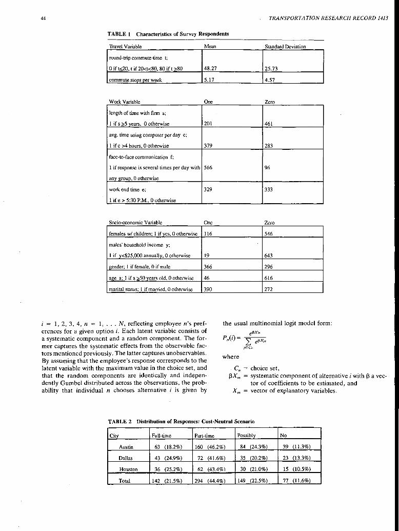
44 TRANSPORTATION RESEARCH RECORD 1413

TABLE 1 Characteristics of Survey Respondents

Travel Variable Mean Standard Deviation

round-trip commute time t;

0 if t.$.20, t if 20<t<80, 80 if t >80 48.27 25.73

commute stops per week 5.17 4.57

Work Variable One Zero

length of time with firm s;

1 ifs >5 years, 0 otherwise 201 461

avg. time using computer per day c;

1 if c >4 hours, 0 otherwise 379 283

face-to-face communication f;

1 if response is several times per day with 566 96

any group, 0 otherwise

work end time e; 329 333

1 if e > 5:30 P.M., 0 otherwise

Socio-economic Variable One Zero

females w/ children; 1 if yes, 0 otherwise 116 546

males' household income y;

1 if y<$25,000 annually, 0 otherwise 19 643

gender; 1 if female, 0 if male 366 296

age a; 1 if a >50 years old, 0 otherwise 46 616

marital status; 1 if married, 0 otherwise 390 272

i = 1, 2, 3, 4, n = 1, ... N, reflecting employee n's pref­erences for a given option i. Each latent variable consists of a systematic component and a random component. The for­mer captures the systematic effects from the observable fac­tors mentioned previously. The latter captures unobservables. By assuming that the employee's response corresponds to the latent variable with the maximum value in the choice set, and that the random components are identically and indepen­dently Gumbel distributed across the observations, the prob­ability that individual n chooses alternative i is given by

the usual multinomial logit model form:

e13Xin

p (i)= -=--n 2: el3Xjn

jECn

where

. en = choice set, j3X;n = systematic component of alternative i with j3 a vec­

tor of coefficients to be estimated, and X;n = vector of explanatory variables.

TABLE 2 Distribution of Responses: Cost-Neutral Scenario

Citv Full-time Part-time Possibly No

Austin 63 (18.2%) 160 (46.2%) 84 (24.3%) 39 (11.3%)

Dallas 43 (24.9%) 72 (41.6%) 35 (20.2%) 23 (13.3%)

Houston 36 (25.2%) 62 (43.4%) 30 (21.0%) 15 (10.5%)

Total 142 (21.5%) 294 (44.4%) 149 (22.5%) 77 (11.6%)

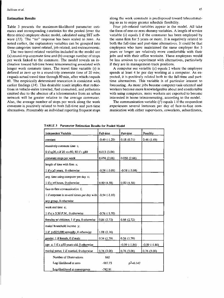
Sullivan et al.

Estimation Results

Table 3 presents the maximum-likelihood parameter esti­mates and corresponding t-statistics for the pooled (over the three cities) employee choice model, calculated using SST soft­ware (13). The "no" response has been scaled to zero. As noted earlier, the explanatory variables can be grouped into three categories: travel related, job related, and socioeconomic.

The two travel-related variables included in the model are (a) round-trip commute time and (b) average number of stops per week linked to the commute. The model reveals an in­clination toward full-time home telecommuting associated with longer work commute times. The travel time variable (t) is defined as zero up to a round-trip commute time of 20 min; t equals actual travel time through 80 min, after which t equals 80. The empirically determined truncation is consistent with earlier findings (14). This desirable result implies that reduc­tions in vehicle-miles traveled, fuel consumed, and pollutants emitted due to the absence of a telecommuter from an urban network will be greater relative to the average commuter. Also, the average number of stops per week along the work commute is positively related to both full-time and part-time alternatives. Presumably an individual reporting frequent stops

45

along the work commute is predisposed toward telecommut­ing so as to enjoy greater schedule flexibility.

Four job-related variables appear in the model. All take the form of one-or-zero dummy variables. A length of service variable (s) equals 1 if the commuter has been employed by the same firm for 5 years or more. It is negatively related to both the full-time and part-time alternatives. It could be that employees who have maintained the same employer for 5 years or longer are relatively more comfortable with their jobs and with their office worksite. These employees would be less anxious to experiment with alternatives, particularly if they are in management-track positions.

A computer use variable (c) equals 1 where the employee spends at least 4 hr per day working at a computer. As ex­pected, it is positively related both to the full-time and part­time alternatives. This variable is of particular interest to forecasting. As more jobs become computer-task-oriented and workers become more knowledgeable about and comfortable with using computers, more workers are expected to become interested irt home telecommuting, according to the model.

The communication variable (f) equals 1 if the respondent experiences several instances per day of face-to-face com­munication with either supervisors, coworkers, subordinates,

TABLE 3 Parameter Estimation Results for Pooled Model

Independent Variable Full-time Part-time Possibly

constant -0.49 (-1.20) 0.18 (0.71) 0.46 (1.69)

round-trip commute time t;

0 if t~20, t if 20 <t<80, 80 if t ~80 0.013 (3.04)

commute stops per week 0.058 (2.66) 0.058 (2.66)

length of time with finn s;

1 if s ~5 years, 0 otherwise -0.58 (-3.08) -0.58 (-3.08)

avg. time using computer per day c;

1 if c >4 hours, 0 otherwise 0.80 (4.58) 0.80 (4.58)

face-to-face communication f;

1 if response is several times per day with -0.54 (-2.10)

any group, 0 otherwise

work end time e;

1 if e > 5:30 P.M., 0 otherwise -0.76 (-3.70)

females w/ children; 1 if yes, 0 otherwise 0.86 (2.72) 0.86 (2.72)

males' household income y;

1 if y<$25,000 annually, 0 otherwise 1.08 (2.16)

gender; 1 if female, 0 if male 0.34 (1.79) 0.34 (1.79)

age a; 1 if a ~50 years old, 0 otherwise -0.59 (-1.86) -0.59 (-1.86)

marital status; 1 if married, 0 otherwise 0.76 (3.00) 0.76 (3.00) 0.76 (3.00)

Number of Observations 662

Log-likelihood at zero -917.73 p2=0.147

Log-likelihood at convergence -782.91

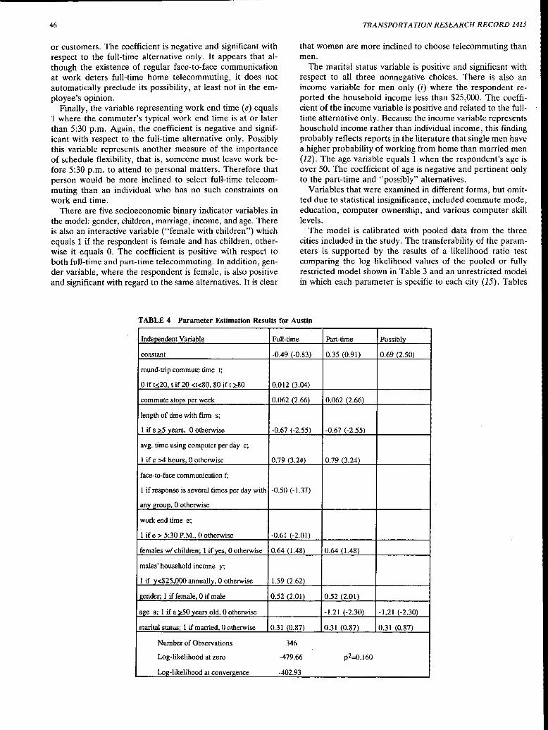
46

or customers. The coefficient is negative and significant with respect to the full-time alternative only. It appears that al­though the existence of regular face-to-face communication at work deters full-time home telecommuting, it does not automatically preclude its possibility, at least not in the em­ployee's opinion.

Finally, the variable representing work end time (e) equals 1 where the commuter's typical work end time is at or later than 5:30 p.m. Again, the coefficient is negative and signif­icant with respect to the full-time alternative only. Possibly this variable represents another measure of the importance of schedule flexibility, that is, someone must leave work be­fore 5:30 p.m. to attend to personal matters. Therefore that person would be more inclined to select full-time telecom­muting than an individual who has no such constraints on work end time.

There are five socioeconomic binary indicator variables in the model: gender, children, marriage, income, and age. There is also an interactive variable ("female with children") which equals 1 if the respondent is female and has children, other­wise it equals 0. The coefficient is positive with respect to both full-time and part-time telecommuting. In addition, gen­der variable, where the respondent is female, is also positive and significant with regard to the same alternatives. It is clear

TRANSPORTATION RESEARCH RECORD 1413

that women are more inclined to choose telecommuting than men.

The marital status variable is positive and significant with respect to all three . nonnegative choices. There is also an income variable for men only (i) where the respondent re­ported the household income less than $25,000. The coeffi­cient of the income variable is positive and related to the'full­time alternative only. Because the income variable represents household income rather than individual income, this finding probably reflects reports inthe literature that single men have a higher probability of working from home than married men (12). The age variable equals 1 when the respondent's age is over 50. The coefficient of age is negative and pertinent only to the part-time and "possibly" alternatives.

Variables that were examined in different forms, but omit­ted due to statistical insignificance, included commute mode, education, computer ownership, and various computer skill levels.

The model is calibrated with pooled data from the three cities included in the study. The transferability of the param­eters is supported by the results of a likelihood ratio test comparing the log likelihood values of the pooled or fully restricted model shown in Table 3 and an unrestricted model in which each parameter is specific to each city (15). Tables

TABLE 4 Parameter Estimation Results for Austin

Indeoendent Variable Full-time Part-time Possibly

constant -0.49 (-0.83) 0.35 (0.91) 0.69 (2.50)

round~trip commute time t;

0 if t~20, t if 20 <t<80, 80 if t ~80 0.012 (3.04)

commute stops per week 0.062 (2.66) 0.062 (2.66)

length of time with firm s;

1 if s ~5 years, 0 otherwise -0.67 (-2.55) -0.67 (-2.55)

avg. time using computer per day c;

1 if c >4 hours, 0 otherwise 0.79 (3.24) 0.79 (3.24)

face-to-face communication f;

1 if response is several times per day with -0.50 (-1.37)

any group, 0 otherwise

work end time e;

1 if e > 5:30 P.M., 0 otherwise -0.61 (-2.01)

females w/ children; 1 if yes, 0 otherwise 0.64 (1.48) 0.64 (1.48)

males' household income y;

1 if y<$25,000 annually, 0 otherwise 1.59 (2.62)

gender; 1 if female, 0 if male 0.52 (2.01) 0.52 (2.01)

age a; 1 if a ~50 years old, 0 otherwise -1.21 (-2.30) -1.21 (-2.30)

marital status; 1 if married, 0 otherwise 0.31 (0.87) 0.31 (0.87) 0.31 (0.87)

Number of Observations 346

Log-likelihood at zero -479.66 p2=0.160

Log-likelihood at convergence -402.93

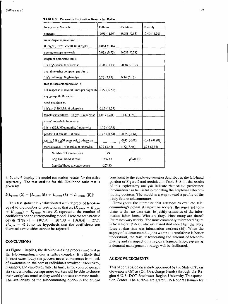
Sullivan et al. 47

TABLE 5 Parameter Estimation Results for Dallas

Independent Variable Full-time Part-time Possibly

constant -0.99 (-1.07) 0.081 (0.18) -0.40 (-1.16)

round-trip commute time t;

0 if t~20, t if 20 <t<80, 80 if t ~80 0.014 (1.46)

commute stops per week 0.032 (0.73) 0.032 (0.73)

length of time with firm s;

1 if s ~5 years, 0 otherwise -0.46 (-1.17) -0.46 (-1.17)

avg. time using computer per day c;

1 if c >4 hours, 0 otherwise 0.76 (2.15) 0.76 (2.15)

face-to-face communication f;

1 if response is several times per day with -0.27 (-0.51)

any group, 0 otherwise

work end time e;

1 if e > 5:30 P.M., 0 otherwise -0.89 (-2.27)

females w/ children; 1 if yes, 0 otherwise 1.06 (1.78) 1.06 (1.78)

males' household income y;

1 if y<$25,000 annually, 0 otherwise -0.39 (-0.33)

gender; ·1 if female, 0 if male -0.25 (-0.64) -0.25 (-0.64)

age a; 1 if a ~50 years old, 0 otherwise -0.42 (-0.80) -0.42 (-0.80)

marital status; 1 if married, 0 otherwise 1.72 (3.44) 1.72 (3.44) 1.72 (3.44)

Number of Observations

Log-likelihood at zero

Log-likelihood at convergence

4, 5, and 6 display the model estimation results for the cities separately. The test statistic for this likelihood ratio test is given by

2{Lpooled (J3) - [LAustin (J3) + LDallas (J3) + LHouston (J3)]}

This test statistic is x2 distributed with degrees of freedom equal to the number ofrestrictions, that is, (KAustin + Koauas

+ KHouston) - Kpooled• where Kj represents the number of coefficients on the corresponding model. Here the test statistic equals 2[782.91 - (402.93 + 207.30 + 158.83)] = 27.7. x2

28 ,.05 = 41.3, so the hypothesis that the coefficients are identical across cities cannot be rejected.

CONCLUSIONS

As Figure 1 implies, the decision-making process involved in the telecommuting choice is rather complex. It is likely that in most cases today the process never commences from lack of awareness on the part of individuals involved: executives, managers, and employees alike. In time, as the concept spreads via various media, perhaps more workers will be able to choose their workplace much as they would choose a commute mode. The availability of the telecommuting option is the crucial

173

-239.83 p2=0.136

-207.30

constraint to the employee decision described in the left-hand portion of Figure 2 and modeled in Table 3. Still, the results of this exploratory analysis indicate that stated preference information can be useful in modeling the employee telecom­muting decision. The model is a step toward a profile of the likely future telecommuter.

Throughout the literature that attempts to evaluate tele­commuting's potential impact on society, the universal com­plaint is that no data exist to justify estimates of the infor­mation labor force. Who are they? How many are there? Estimates vary widely. The most commonly referenced figure is from Porat (1977), who estimated that about half the labor force at that time was information workers (16). When the supply of telecommutable jobs within the workforce is better understood, the task of forecasting the amount of telecom­muting and its impact on a region's transportation system as a demand management strategy will be facilitated.

ACKNOWLEDGMENTS

This paper is based on a study sponsored by the State of Texas Governor's Office (Oil Overcharge Funds) through the Re­gion 6 U.S. DOT Southwest Region University Transporta­tion Center. The authors are grateful to Robert Herman for

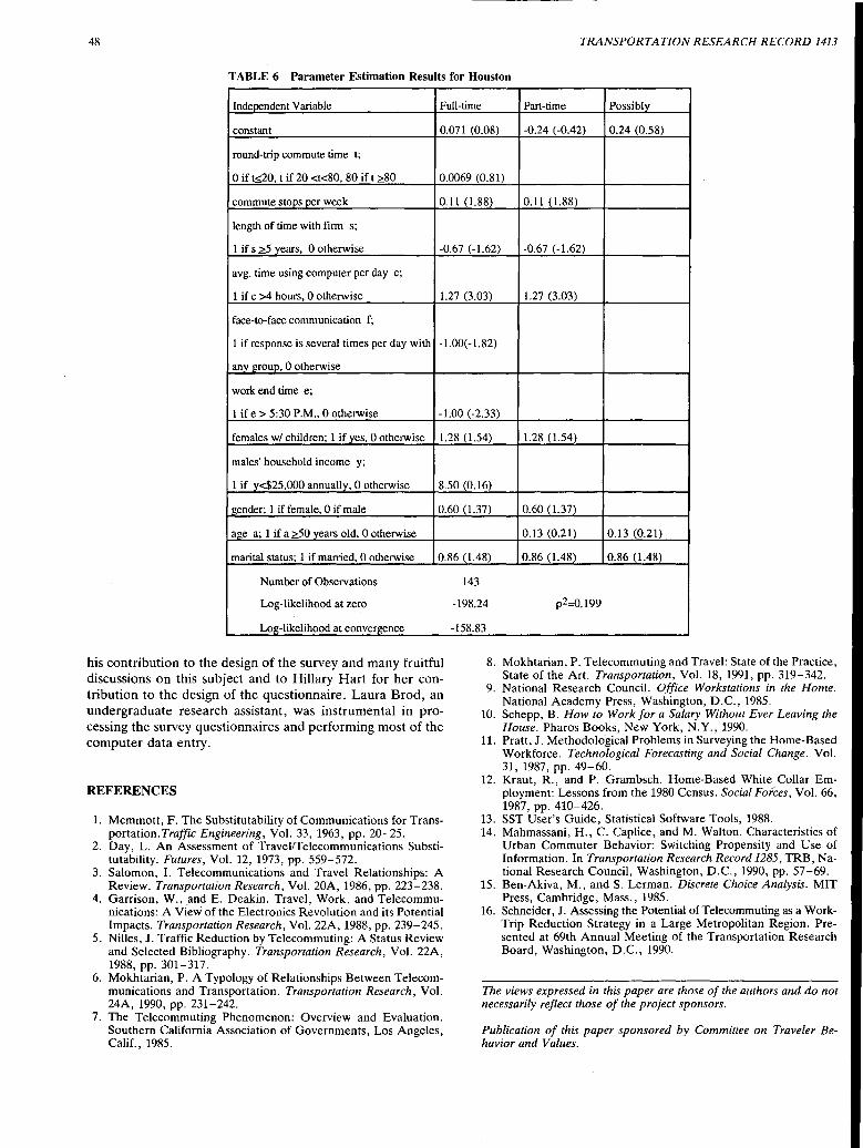
48 TRANSPORTATION RESEARCH RECORD 1413

TABLE 6 Parameter Estimation Results for Houston

Independent Variable Full-time Part-time Possibly

constant 0.071 (0.08) -0.24 (-0.42) 0.24 (0.58)

round-trip commute time t;

0 if t<20, t if 20 <t<80, 80 if t >80 0.0069 (0.81)

commute stoos oer week 0.11 (1.88) 0.11(1.88)

length of time with firm s;

1 if s ~5 years, 0 otherwise -0.67 (-1.62) -0.67 (-1.62)

avg. time using computer per day c;

1 if c >4 hours, 0 otherwise 1.27 (3.03) 1.27 (3.03)

face-to-face communication f;

1 if response is several times per day with -1.00(-1.82)

any group, 0 otherwise

work end time e;

1 if e > 5:30 P.M., 0 otherwise -1.00 (-2.33)

females w/ children; 1 if yes, 0 otherwise 1.28 (1.54) 1.28 (1.54)

males' household income y;

1 if v<$25,000 annually, 0 otherwise 8.50 (0.16)

gender; 1 if female, 0 if male 0.60 (1.37) 0.60 (l.37)

age a; 1 if a ~50 years old, 0 otherwise 0.13 (0.21) 0.13 (0.21)

marital status; 1 if married, 0 otherwise 0.86 (1.48) 0.86 (l.48) 0.86 (1.48)

Number of Observations

Log-likelihood at zero

Log-likelihood at convergence

his contribution to the design of the survey and many fruitful discussions on this subject and to Hillary Hart for her con­tribution to the design of the questionnaire. Laura Brod, an undergraduate research assistant, was instrumental in pro­cessing the survey questionnaires and performing most of the computer data entry.

REFERENCES

1. Memmott, F. The Substitutability of Communications for Trans­portation.Traffic Engineering, Vol. 33, 1963, pp. 20-25.

2. Day, L. An Assessment of Travel/Telecommunications Substi­tutability. Futures, Vol. 12, 1973, pp. 559-572.

3. Salomon, I. Telecommunications and Travel Relationships: A Review. Transportation Research, Vol. 20A, 1986, pp. 223-238.

4. Garrison, W., .and E. Deakin. Travel, Work, and Telecommu­nications: A View of the Electronics Revolution and its Potential Impacts. Transportation Research, Vol. 22A, 1988, pp. 239-245.

5. Nilles, J. Traffic Reduction by Telecommuting: A Status Review and Selected Bibliography. Transportation Research, Vol. 22A, 1988, pp. 301-317.

6. Mokhtarian, P. A Typology of Relationships Between Telecom­munications and Transportation. Transportation Research, Vol. 24A, 1990, pp. 231-242.

7. The Telecommuting Phenomenon: Overview and Evaluation. Southern California Association of Governments, Los Angeles, Calif., 1985.

143

-198.24 p2=0.199

-158.83

8. Mokhtarian, P. Telecommuting and Travel: State of the Practice, State of the Art. Transportation, Vol. 18, 1991, pp. 319-342.

9. National Research Council. Office Workstations in the Home. National Academy Press, Washington, D.C., 1985.

10. Schepp, B. How to Work for a Salary Without Ever Leaving the House. Pharos Books, New York, N.Y., 1990.

11. Pratt, J. Methodological Problems in Surveying the Home-Based Workforce. Technological Forecasting and Social Change. Vol. 31, 1987, pp. 49-60.

12. Kraut, R., and P. Grambsch. Home-Based White Collar Em­ployment: Lessons from the 1980 Census. Social Forces, Vol. 66, 1987, pp. 410-426.

13. SST User's Guide, Statistical Software Tools, 1988. 14. Mahmassani, H., C. Caplice, and M. Walton. Characteristics of

Urban Commuter Behavior: Switching Propensity and Use of Information. In Transportation Research Record 1285, TRB, Na­tional Research Council, Washington, D.C., 1990, pp. 57-69.

15. Ben-Akiva, M., and S. Lerman. Discrete Choice Analysis. MIT Press, Cambridge, Mass., 1985.

16. Schneider, J. Assessing the Potential of Telecommuting as a Work­Trip Reduction Strategy in a Large Metropolitan Region. Pre­sented at 69th Annual Meeting of the Transportation Research Board, Washington, D.C., 1990.

The views expressed in this paper are those of the authors and do not necessarily reflect those of the project sponsors.

Publication of this paper sponsored by Committee on Traveler Be­havior and Values.

TRANSPORTATION RESEARCH RECORD 1413 49

Modeling Rail Access Mode and Station Choice

KAI-SHENG FAN, ERIC J. MILLER, AND DANIEL BADOE

Access mode and station choice by commuter rail and subway users are modeled using morning peak-period work trip com­muting in the greater Toronto, Ontario, area as a case study. Based on observed station choice behavior, rules for determining access station choice sets for both commuter rail and subway were developed. For commuter rail, the two closest stations on the two closest lines (relative to the worker's place of residence) define the access station choice set. For.automobile access to the subway, the five closest subway stations define the choice set. A nested logit model of commuter rail access mode and station and a multinomial logit model of subway automobile access station choice were then developed. Consistent with the findings of other researchers, credible models of access mode and station choice were obtained. Directions identified for further work include test­ing alternative overall main mode plus access choice structures, properly capturing parking supply and price effects with these models, developing improved representations of the automobile passenger mode, and development of improved network mod­eling software for dealing with "mixed" modes of travel.

As urban areas continue to suburbanize, transit work trips increasingly become multimodal_ in nature. That is, a typical trip may consist of driving to a commuter rail station, taking the commuter train into a central station, and then taking the subway to the final destination. The access mode for com­muter rail and subway trips for suburban residents is an in­creasingly impfiltant component of the overall "choice bun­dle" facing these commuters. This importance is reflected in the emphasis that many suburban transit properties place on providing feeder services to rail systems. It is also reflected in the emphasis that many jurisdictions place on the concept of "gateways," that is, points at which automobile users can be intercepted and encouraged to leave their cars and com­plete their journey by public transit. In addition, the provision and pricing of parking at commuter rail and subway stations are ongoing concerns to most rail operators.

Given the inevitable continuing suburbanization of North American commuting patterns, the importance of rail services can be expected to grow significantly over the forseeable fu­ture. Thus, credible forecasts of expected rail ridership at­tracted from these growing suburban areas are essential to planning activities. Such forecasts are, however, difficult to generate without a proper understanding of the access com­ponent of the trip. Unfortunately, the current modeling state of practice does not adequately address the access mode ques­tion, either in terms of representing the access mode choices being made by commuters or in terms of representing the impact that changes in access mode characteristics will have

Department of Civil Engineering, University of Toronto, Toronto, Canada M5S 1A4.

on line-haul mode choices. The purpose of this paper is to explore this problem in depth.

LITERATURE REVIEW

Few explicit models of rail access mode and station choice are reported in the literature. Kumar and Gur (1) present a sequence of logit models that predict choices among auto­mobile and transit, rail, and express bus given the use of transit and the choices among walk, bus, park-and-ride, and kiss-and-ride access to the chosen line-haul mode. This model, however, is not fully consistent with random utility choice theory and does not deal explicitly with the question of access station choice. Sargious and Janarthanan (2) report a simple logit model developed for Calgary, Alberta, for the choice among automobile, transit all-way, and park-and-ride for work trips. Access stations are assumed to be chosen on a "least cost" basis.

In the late 1970s, Talvitie (3) developed a model of the joint choice of access mode (walk, bus, drive, kiss-and-ride) and access station for Bay Area Rapid Transit (BART). Up to three access stations were considered per origin zone, based on stations observed to be chosen by workers living in a given zone. Important conclusions from this paper include (a) the kiss-and-ride mode proved very difficult to model adequately, (b) the joint model did not demonstrate significant violations of the independence of irrelevant alternatives (IIA property), and ( c) proper representation of the access network is critical to access mode and station choice model development.

Mukundan et al. ( 4) present a nested logit model of Wash­ington, D .C., Metro rail access mode and station choice. This model assumes access mode (walk, bus, automobile drive, automobile passenger) as the upper-level choice, with access station as the lower-level choice, conditional on the access mode choice. The two best access stations for the walk mode and the six best stations for the other three modes were used to define the access station choice set, where "best" is defined in terms of predetermined modal "impedance" functions. Similar to Talvitie's findings, the automobile passenger mode proved difficult to model.

Miller and Cheah (5) present a multinomial logit model of work trip mode choice for the Greater Toronto Area (GTA). The model includes six modes: (a) automobile (drive or pas­senger), (b) transit with walk access, (c) subway with auto­mobile access, (d) commuter rail with transit or walk access, (e) commuter rail with automobile access, and (f) walk all­way. The commuter rail access station that provides the maxi­mum utility for the trip is chosen for each commuter rail mode.

50

The subway automobile access station is specified for a given origin zone based on patterns of station use observed in ri­dership surveys. No test for IIA violations within this joint access and line-haul mode choice model was performed.

At least three issues are raised by this brief review. First, to date, little empirical investigation into access station choice set definition appears to have been performed. Second, little explicit investigation into access mode and station decision structure has been undertaken. Talvitie's results support his assumed joint decision structure. Mukundan et al. 's results, on the other hand, support an assumed nested decision struc­ture. Finally, practical issues associated with coding access network components and incorporation of access mode and station calculations within available modeling software, among others, are critical to the development of access mode-station models and to their practical application within operational planning models.

DESCRIPTION OF DATA

The GT A, which is the study area for this paper, provides a good opportunity to study rail access mode and station choice issues because it contains both commuter rail and subway systems, which both compete with and complement one an­other in providing essentially radial service into the Toronto Central Area.

The commuter rail system for the GTA, GO-Rail, is a radial system, focused on Union Station, located at the southern end of Toronto's Central Area (see Figure 1). Union Station is also a major station of Toronto's subway system, thereby providing convenient transit connections between the com­muter rail system and downtown Toronto. The GO-Rail sys­tem is primarily designed to carry commuters from residential suburban areas lying outside metropolitan Toronto to em­ployment locations within downtown Toronto. On-board sur­veys of GO-Rail riders are performed every 2 years. The travel choice data used in this paper are obtained from the 1987 survey.

Subway access is treated differently from commuter rail access in this paper in that only subway access station choice is modeled, given that the automobile is used as the access mode. This approach is based on the following assumptions:

• Surface transit access to subway is not a sufficiently dis­tinct "choice bundle" relative to taking surface transit for the entire trip that- it requires explicit representation· within the set of modal alternatives,

• Subway access station choice for surface transit is ade­quately modeled within current transit assignment proce­dures, and

• The key distinction that needs to be made within the work trip mode choice model is, therefore, between the "transit all-way" mode and the "transit part-way, auto part-way" mode (i.e., automobile access to the subway). Data from the 1986 Transportation Tomorrow Survey (TTS) were used in the analysis of subway automobile access station choice behavior. Figure 2 shows the location of the 12 park-and-ride stations within the subway system. This study focusses on six of these stations (Finch, Kipling, Islington, Kennedy, Wilson, and Mccowan, in order of use), which are used by most automobile­access subways users.

TRANSPORTATION RESEARCH RECORD 1413

All level of service data required for model development were generated using computerized representations of the GT A automobile and transit networks maintained within the EMME/2 modeling system.

DETERMINING ACCESS STATION CHOICE SETS

Commuter Rail Access Station Choice Sets

Figure 3a presents approximate access "catchment areas" for each GO-Rail station, as defined by the home ends of trips using each station, given that the tripmaker used the auto­mobile access mode (as either a driver or a passenger). These catchment areas were constructed by first deleting the 5 per­cent longest trips in the sample (so as to eliminate unnecessary clutter in the plot) and then identifying the trip origin furthest from the given access station for each 30-degree arc segment. These "furthest points" were connected to form the catch­ment area.

Significant overlap exists among these catchment areas, in­dicating that not all trip makers use their closest access station and that trip makers traveling from approximately the same home locations make different access station choices. These results imply that more than one access station must, in gen­eral, be included in trip makers' choice sets and that selection of an access station is likely to be best modeled probabilist­ically. Figure 3b presents similar information for rail com­muters using transit access to the system. This plot is generally far simpler than the one for automobile access users, indi­cating that a large number of transit access users travel to their nearest station. Nevertheless, sufficient overlap among catchment areas exists to indicate that transit users' access station choice should also be modeled probabilistically.

Various cross-tabulations were performed in the search for any systematic structure in the distribution of chosen access stations. This analysis ultimately resulted in Table 1, which tabulates the observed station choices with respect to the closeness of the chosen line to the traveler's home. "Close­ness" is simply defined on the basis of the straightline distance between home and stations on the given line. Thus, the "clos­est" line is the one containing the absolute closest station. From Table 1, 98.8 percent of the observed trip makers use an access station on the rail line that is either closest or second closest to their homes, while 94.5 percent use either the first­closest or second-closest station on either the first- or second­closest line. Table 1 presents this same information- broken down by access mode, which indicates that these results hold by access mode as well. These results suggest that a simple rule for determining the access station choice set is to include the two closest stations on the two closest lines, where dis­tances are calculated on a straightline basis. This simple rule accounts for virtually 95 percent of observed behavior on a station basis, while it accounts for almost 99 percent of ob­served behavior on a line basis.

Subway Auto Access Station Choice Sets

Figure 4 plots the spatial distribution of subway park-and­ride station automobile access origin (home) locations for the

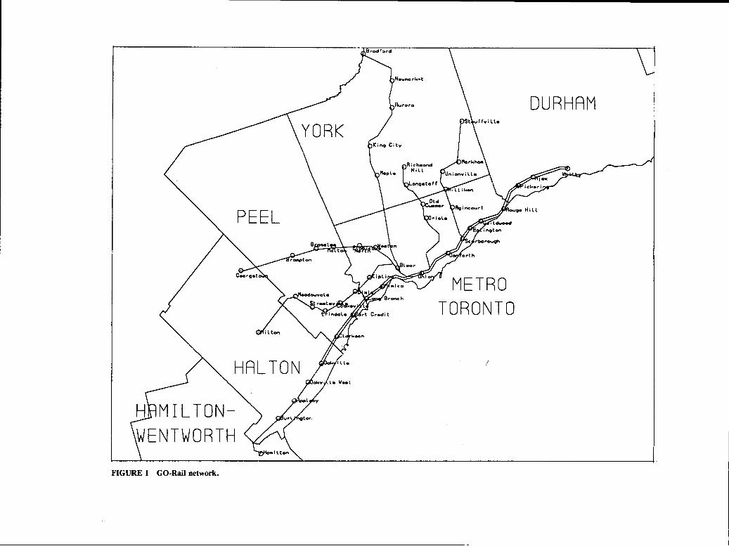
PEEL

FIGURE 1 GO-Rail network.

METRO TORONTO

DURHAM

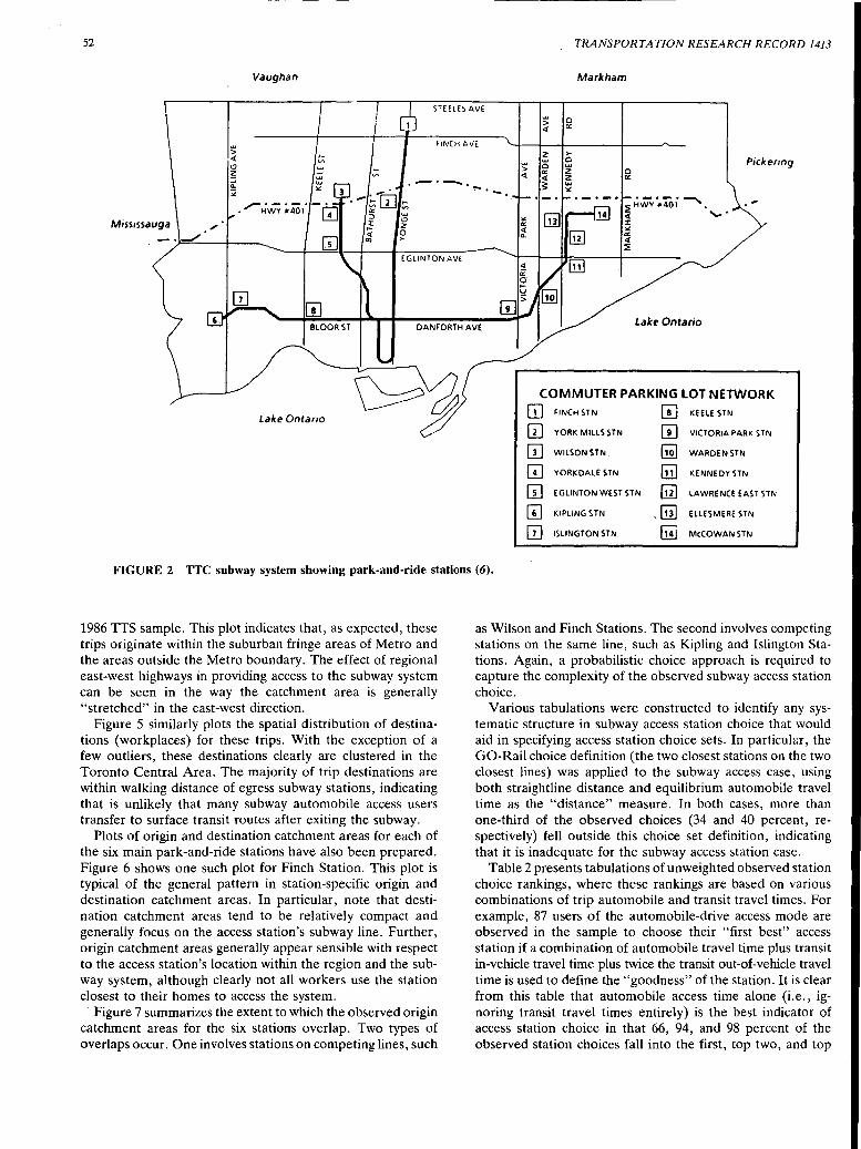
52 TRANSPORTATION RESEARCH RECORD 1413

Vaughan Markham

STEELE~ AVE

> 0 <( a:

FINCH AVt z >-

.... 0 8 Pickering > a: z 0 <( <( ~ a:

·-. ~ :..:

~Hwv',.4oi ~

"' [ii] <( a: ::c <( rw :..: Q. a:

<(

~ EGLINTON AVE

DANFORTH AVE Lake Ontario

COMMUTER PARKING LOT NETWORK

Lake Ontario [!] FINCH STN [!] KEELE STN

[l] YORK MILLS STN [iJ VICTORIA PARK STl\i

[l] WILSON STN.. [!Q] WARDEN STN

G] YORKDALE STN [ii] KENNEDY STN

Ci] EGLINTON WEST STN [W LAWRENCE EAST STN

[!] KIPLING STN . [ii] ELLESMERE STN

[1J ISLING TON STN. [!!J McCOWAN STN

FIGURE 2 TTC subway system showing park-and-ride stations (6).

1986 TIS sample. This plot indicates that, as expected, these trips originate within the suburban fringe areas of Metro and the areas outside the Metro boundary. The effect of regional east-west highways in providing access to the subway system can be seen in the way the catchment area is generally "stretched" in the east-west direction.

Figure 5 similarly plots the spatial· distribution of destina­tions (workplaces) for these trips. With the exception of a few outliers, these destinations clearly are clustered in the Toronto Central Area. The majority of trip destinations are within walking distance of egress subway stations, indicating that is unlikely that many subway automobile access users transfer to surface transit routes after exiting the subway.

Plots of origin and destination catchment areas for each of the six main park-and-ride stations have also been prepared. ·Figure 6 shows one such plot for Finch Station. This plot is typical of the general pattern in station-specific origin and destination catchment areas. In particular, note that desti­nation catchment areas tend to be relatively compact and generally focus on the access station's subway line. Further, origin catchment areas generally appear sensible with respect to the access station's location within the region and the sub­way system, although clearly not all workers use the station closest to their homes to access the system.

Figure 7 summarizes the extent to which the observed origin catchment areas for the six stations overlap. Two types of overlaps occur. One involves stations on competing lines, such

as Wilson and Finch Stations. The second involves competing stations on the same line, such as Kipling and Islington Sta­tions. Again, a probabilistic choice approach is required to capture the complexity of the observed subway access station choice.

Various tabulations were constructed to identify any sys­tematic structure in subway access station choice that would aid in specifying access station choice sets. In particular, the GO-Rail choice definition (the two closest stations on the two closest lines) was applied to the subway access case, using both straightline distance and equilibrium automobile travel time as the "distance" measure. In both cases, more than one-third of the observed choices (34 and 40 percent, re­spectively) fell outside this choice set definition, indicating that it is inadequate for the subway access station case.

Table 2 presents tabulations of unweighted observed station choice rankings, where these rankings are based on various combinations of trip automobile and transit travel times. For example, 87 users of the automobile-drive access mode are observed in the sample to choose their "first best" access station if a combination of automobile travel time plus transit in-vehicle travel time plus twice the transit out-of-vehicle travel time is used to define the "goodness" of the station. It is clear from this table that automobile access time alone (i.e., ig­noring transit travel times entirely) is the best indicator of access station choice in that 66, 94, and 98 percent of the observed station choices fall into the first, top two, and top

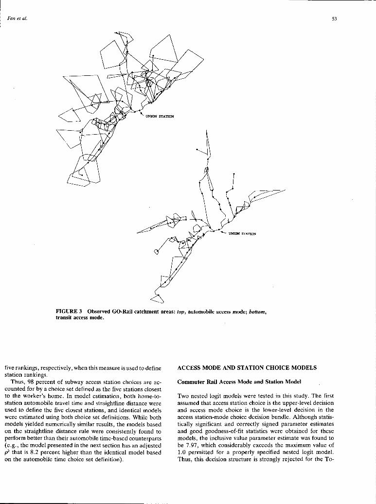
Fan et al. 53

'UNION STATION

....._ UNION S"fATION

FIGURE 3 Observed GO-Rail catchment areas: top, automobile access mode; bottom, transit access mode.

five rankings, respectively, when this measure is used to define station rankings.

Thus, 98 percent of subway access station choices are ac­counted for by a choice set defined as the five stations closest to the worker's home. In model estimation, both home-to­station automobile travel time and straightline distance were used to define the five closest stations, and identical models were estimated using both choice set definitions. While both models yielded numerically similar results, the models based on the straightline distance rule were consistently found to perform better than their automobile time-based counterparts (e.g., the model presented in the next section has an adjusted p2 that is 8.2 percent higher than the identical model based on the automobile time choice set definition).

ACCESS MODE AND STATION CHOICE MODELS

Commuter Rail Access Mode and Station Model

Two nested logit models were tested in this study. The first assumed that access station choice is the upper-level decision and access mode choice is the lower-level decision in the access station-mode choice decision bundle. Although statis­tically significant and correctly signed parameter estimates and good goodness-of-fit statistics were obtained for these models, the inclusive value parameter estimate was found to be 7.97, which considerably exceeds the maximum value of 1.0 permitted for a properly specified nested logit model. Thus, this decision structure is strongly rejected for the To-

TABLE 1 Access Station Choice (Percent of Total Trips) by Line and Station

Auto and Transit Access Modes (Total Trips: 10875)

LINE1 STATION3 Closest 2nd Closest Other Total

Closest Line 73.51 13.40 3.90 90.80 2nd Closest Line 6.45 1.16 0.34 7.94 Other 0.00 0.00 1.25 1.25

Total 79.95 14.56 5.49 100.00%

Auto Access Mode

LINE STATION Closest 2nd Closest Other Total

Closest Line 67.31 15.90 4.93 88.14 2nd Closest Line 8.15 1.57 0.45 10.17 Other 0.00 0.00 1.69 1.69

Total 75.46 17.48 7.06 100.00%

Transit Access Mode

LINE STATION Closest 2nd Closest Other Total

Closest Line 81.55 11.70 2.43 95.69 2nd Closest Line 3.83 0.27 0.05 4.15 Other 0.00 0.00 0.16 0.16

Total 85.38 11.97 2.64 100.00%

Notes:

1. Indicates the percentage of rail passengers who access the line closest to their home, second closest, etc.; e.g., 90.8% of the observed passengers use the rail line that is closest to their homes.

2. Indicates the percentage of rail passengers who access the closest station to their home, the second closest station, etc., given the chosen rail line. For example, 73.51 % of all rail passengers use the closest station on the closest line, while 13.4% use the second closest station on their closest line (note that this station need not be the second closest station_ overall, it is defined conditional on the chosen line).

FIGURE 4 Subway automobile access origin catchment area, six major park-and-ride stations.

e e e e

FIGURE 5 Subway automobile access destination catchment area, six major park-and-ride stations.

ronto data base in favor of the second nested model consid­ered, where access mode is the upper-level choice and access station is the lower-level choice, conditional on access mode choice. The following estimation results are based on this latter decision structure.

Table 3 presents the variables included in the final speci­fication of the lower-level access station model. This model applies to the automobile and transit access modes (GO-Rail stations are sufficiently far apart that at most one station will be within feasible walking distance of a worker's home) and­was estimated as an ordinary multinomial logit model, con­ditional on access mode choice. This yields consistent but somewhat inefficient parameter estimates. The combination of access and line-haul in-vehicle travel time is used on the basis of previous estimation results in which the access and line-haul travel time parameters were generally found not to have statistically different parameter estimates [this is also consistent with the findings of Talvitie (3) and Miller and

FIGURE 6 Origin and destination catchment areas, Finch automobile access station.

Cheah (5)]. Statistically reliable, correctly signed parameter estimates could not be obtained for transit out-of-vehicle ac­cess time, automobile access cost, and rail line-haul fares. This was most likely due to insufficient variation in the var­iable values across stations.

A closest station dummy variable is included in the auto­mobile mode station utilities because it yields a significantly improved model, in terms of both goodness of fit and rea­sonableness of the other parameter estimates obtained. Models that exclude a closest station dummy tend to predict that trip makers will use access stations that are closer to their work­places than is actually the case.

Table 4 presents the maximum likelihood estimation results for this model. All variables are statistically significant and correctly signed. The goodness-of-fit statistics are extremely strong, reflecting the tendency of the closest station to dom­inate the process.

Wilson & I\ Islington \\

'(j

Finch & Wilson /

~ Finch & Mccowan

0 Finch & Kennedy

1!1111 Kennedy & Mc:cowon

FIGURE 7 Overlapping origin catchment areas, six major park-and-ride stations.

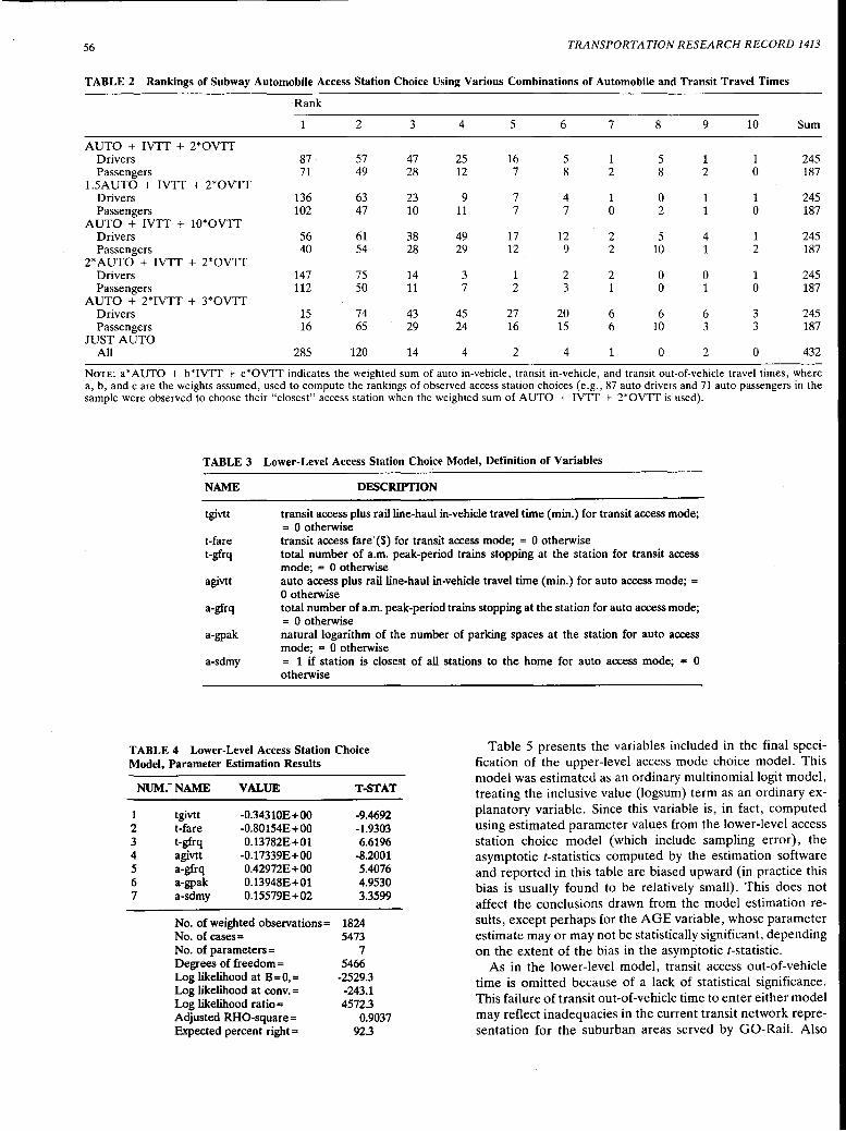
56 TRANSPORTATION RESEARCH RECORD 1413

TABLE 2 Rankings of Subway Automobile Access Station Choice Using Various Combinations of Automobile and Transit Travel Times

·Rank

2 3 4 5 6 7 8 9 10 Sum

AUTO + IVTT + 2*0VTT Drivers 87 57 47 25 16 5 1 5 1 1 245 Passengers 71 49 28 12 7 8 2 8 2 0 187

1.5AUTO + IVTT + 2*0VTT Drivers 136 63 23 9 7 4 1 0 1 1 245 Passengers 102 47 10 11 7 7 0 2 1 0 187

AUTO + IVTT + lO*OVTT Drivers 56 61 38 49 17 12 2 5 4 1 245 Passengers 40 54 28 29 12 9 2 10 1 2 187

2*AUTO + IVTT + 2*0VTT Drivers 147 75 14 3 1 2 2 0 0 1 245 Passengers 112 50 11 7 2 3 1 0 1 0 187

AUTO + 2*IVTT + 3*0VTT Drivers 15 74 43 45 27 20 6 6 6 3 245 Passengers 16 65 29 24 16 15 6 10 3 3 187

JUST AUTO All 285 120 14 4 2 4 0 2 0 432

NOTE: a* AUTO + b*IVTT + c*OVTT indicates the weighted sum of auto in-vehicle, transit in-vehicle, and transit out-of-vehicle travel times, where a, b, and c are the weights assumed, used to compute the rankings of observed access station choices (e.g., 87 auto drivers and 71 auto passengers in the sample were observed to choose their "closest" access station when the weighted sum of AUTO + IVTT + 2*0VTT is used).

TABLE 3 Lower-Level Access Station Choice Model, Definition of Variables

NAME

tgivtt

t-fare t-gfrq

agiytt

a-gfrq

a-gpak

a-sdmy

DF.sCRIPTION

transit access plus rail line-haul in-vehicle travel ti.me (min.) for transit access mode; = 0 otherwise transit access fare'($) for transit access mode; = 0 otherwise total number of a.m. peak-period trains stopping at the station for transit access mode; = 0 otherwise auto access plus rail line-haul in-vehicle travel ti.me (min.) for auto access mode; = 0 otherwise total number of a.m. peak-period trains stopping at the station for auto access mode; = 0 otherwise natural logarithm of the number of parking spaces at the station for auto access mode; = 0 otherwise = 1 if station is closest of all stations to the home for auto access mode; = 0 otherwise

TABLE 4 Lower-Level Access Station Choice Model, Parameter Estimation Results

Table 5 presents the variables included in the final speci­fication of the upper-level access mode choice model. This model was estimated as an ordinary multinomial logit model, treating the inclusive value (logsum) term as an ordinary ex­planatory variable. Since this variable is, in fact, computed using estimated parameter values from the lower-level access station choice model (which include sampling error), the asymptotic t-statistics computed by the estimation software and reported in this table are biased upward (in practice this bias is usually found to be relatively small). This does not affect the conclusions drawn from the model estimation re­sults, except perhaps for the AGE variable, whose parameter estimate may or may not be statistically significant, depending on the extent of the bias in the asymptotic t-statistic.

1 2 3 4 5 6 7

NUM."'NAME

tgivtt t-fare t-gfrq agivtt a-gfrq a-gpak a-sdmy

VALUE

-0.34310E+OO -0.80154E+ 00 0.13782E+Ol

-0.17339E+OO 0.42972E + 00 0.13948E+Ol 0.15579E + 02

No. of weighted observations= No. of cases= No. of parameters= Degrees of freedom= Log likelihood at B = 0, = Log likelihood at conv. = Log likelihood ratio= Adjusted RHO-square= Expected percent right=

T-sf AT

-9.4692 -1.9303 6.6196

-8.2001 5.4076 4.9530 3.3599

1824 5473

7 5466

-2529.3 -243.1 4572.3

0.9037 92.3

As in the lower-level model, transit access out-of-vehicle time is omitted because of a lack of statistical significance. This failure of transit out-of-vehicle time to enter either model may reflect inadequacies in the current transit network repre­sentation for the suburban areas served by GO-Rail. Also

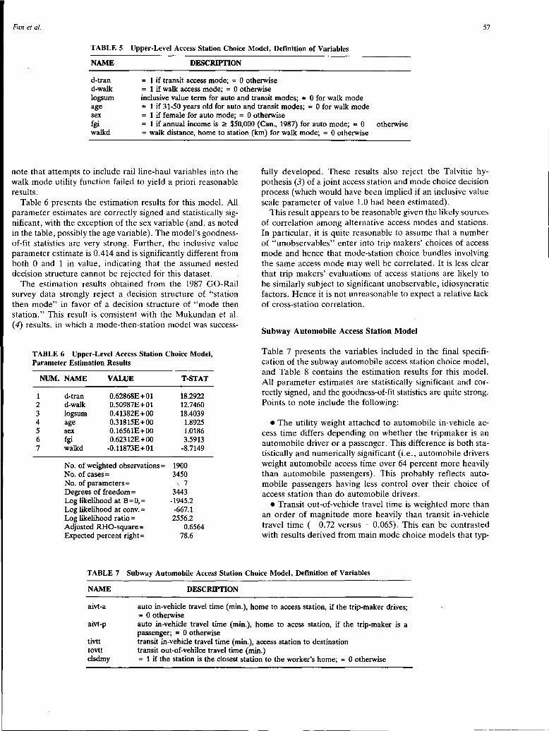
Fan et al. 57

TABLE 5 Upper-Level Access Station Choice Model, Definition of Variables

NAME DFSCRIPI10N

d-tran d-walk logs um age sex

= 1 if transit access mode; = 0 otherwise = 1 if walk access mode; = 0 otherwise inclusive value term for auto and transit modes; = 0 for walk mode = 1 if 31-50 years old for auto and transit modes; = 0 for walk mode = 1 if female for auto mode; = 0 otherwise

fgi walkd

= 1 if annual income is ~ $50,000 (Can., 1987) for auto mode; = 0 otherwise = walk distance, home to station (km) for walk mode; = 0 otherwise

note that attempts to include rail line-haul variables into the walk mode utility function failed to yield a priori reasonable results.

Table 6 presents the estimation results for this model. All parameter estimates are correctly signed and statistically sig­nificant, with the exception of the sex variable (and, as noted in the table, possibly the age variable). The model's goodness­of-fit statistics are very strong. Further, the inclusive value parameter estimate is 0.414 and is significantly different from both 0 and 1 in value, indicating that the assumed nested decision structure cannot be rejected for this dataset.

The estimation results obtained from the 1987 GO-Rail survey data strongly reject a decision structure of "station then mode" in favor of a decision structure of "mode then station." This result is consistent with the Mukundan et al. ( 4) results, in which a mode-then-station model was success-

TABLE 6 Upper-Level Access Station Choice Model, Parameter Estimation Results

NUM. NAME VALUE

1 2 3 4 5 6 7

d-tran 0.62868E+Ol d-walk 0.50987E+Ol logsum 0.41382E + 00 age 0.31815E+OO sex 0.16561E+OO fgi 0.62312E + 00 walkd -0.11873E+01

No. of weighted observations= No. of cases= No. of parameters= Degrees of freedom= Log likelihood at B = 0, = Log likelihood at conv. = Log likelihood ratio= Adjusted RHO-square= Expected percent right=

T-s'TAT

18.2922 12.7460 18.4039 1.8925 1.0186 3.5913

·8.7149

1900 3450 "7

3443 -1945.2 -667.1 2556.2

0.6564 78.6

fully developed. These results also reject the Talvitie hy­pothesis (3) of a joint access station and mode choice decision process (which would have been implied if an inclusive value scale parameter of value 1.0 had been estimated).

This result appears to be reasonable given the likely sources of correlation among alternative access modes and stations. In particular, it is quite reasonable to assume that a number of "unobservables" enter into trip makers' choices of access mode and hence that mode-station choice bundles involving the same access mode may well be correlated. It is less clear that trip makers' evaluations of access stations are likely to be similarly subject to significant unobservable, idiosyncratic factors. Hence it is not unreasonable to expect a relative lack of cross-station correlation.

Subway Automobile Access Station Model

Table 7 presents the variables included in the final specifi­cation of the subway automobile access station choice model, and Table 8 contains the estimation results for this model. All parameter estimates are statistically significant and cor­rectly signed, and the goodness-of-fit statistics are quite strong. Points to note include the following:

• The utility weight attached to automobile in-vehicle ac­cess time differs depending on whether the tripmaker is an automobile driver or a passenger. This difference is both sta­tistically and numerically significant (i.e., automobile drivers weight automobile access time over 64 percent more heavily than automobile passengers). This probably reflects auto­mobile passengers having less control over their choice of access station than do automobile drivers.

•Transit out-of-vehicle travel time is weighted more than an order of magnitude more heavily than transit in-vehicle travel time (-0.72 versus -0.065). This can be contrasted with results derived from main mode choice models that typ-

TABLE 7 Subway Automobile Access Station Choice Model, Definition of Variables

NAME

aivt-a

aivt-p

tivtt tovtt clsdmy

DFSCRIPI10N

auto in-vehicle travel time (min.), home to access station, if the trip-maker drives; = 0 otherwise auto in-vehicle travel time (min.), home to acess station, if the trip-maker is a passenger; = 0 otherwise transit in-vehicle travel time (min.), access station to destination transit out-of-vehilce travel. time (min.) = 1 if the station is the closest station to the worker's home; = 0 otherwise

58

TABLE 8 Subway Automobile Access Station Choice Model, Parameter Estimation Results

NUM. NAME VALUE

1 aivt'a -0.16112E+OO 2 aivt-p -0.97992E-01 3 4 5

tivtt -0.65272E-01 tovtt -0.72376E+ 00 clsdmy 0.10892E+02

No. of weighted observations= No. of cases= No. of parameters= Degrees of freedom= Log likelihood at B = 0, = Log likelihood at conv. = Log likelihood ratio= Adjusted RHO-square= Expected percent right=

T-STAT

-10.45 -7.01 -5.11 -9.63 3.17

1698 6792

5 6787

-2732.9 -1054.3 3357.3

0.6139 67:9

ically indicate a ratio in the range of 2 to 5. This result is consistent, however, with analysis results, not shown in this paper, that strongly indicate that minimization of subway-to­subway transfer times and egress walk times, or both, appear to be significant in explaining access station (line) choice ( 6).

• Parking capacity was not found to be a useful explanatory variable in this model.

• Transit fare is constant across all station alternatives and therefore cannot enter the model. Similarly, subway line fre­quencies and parking charges do not vary sufficiently to war­rant inclusion in the model.

In comparing the subway automobile access model defined by Tables 7 and 8 with the GO-Rail access station model presented in Tables 3 through 6, the following points should be noted:

•A closest station dummy variable seems to be needed in both models, indicating the strong "bias" effect exerted by the closest station. The effect appears to be stronger in the case of GO-Rail access (a parameter value of 15.6 versus 10.9 for subway access), although the two parameter estimates are not statistically different.

•Automobile access time parameter estimates are quite consistent between the two models (-0.173 versus -0.161) and are not statistically different from one another.

• Transit line-haul in-vehicle time appears to be far more significant in the choice of automobile access station for GO­Rail users than for subway users (a utility weight of -0.173 versus -0.0653).

IMPLICATIONS FOR MODEL DEVELOPMENT AND FUTURE WORK

The models presented here assumed a joint, main mode de­cision structure in which GO-Rail and subway with auto­mobile access compete with other main modes, such as au­tomobile all-way, transit all-way,.· and walk all-way. Other decision structures, however, are conceivable and should be statistically tested within the nested logit modeling structure.

TRANSPORTATION RESEARCH RECORD 1413

Overall, the performance of parking supply and·price var­iables in these models was somewhat disappointing. There are several reasons for this result. First, parking charges do not vary significantly from one Toronto Transit Commission lot to another. Thus, they can have little impact on the access· station choice problem. Park-and-ride parking charges are likely to play a more significant role in explaining the choice of the subway with automobile access main mode in which these costs can be compared with the price of parking at the workplace for the drive-all-way mode [this is found to be the case by Miller and Cheah (5)].

Second, the role that parking supply plays within the choice process is likely to be rather complex. Parking supply probably acts as a constraint on access station choice; that is, a traveler cannot use a given station if he or she cannot find a parking space there. Exactly which trip makers are so constrained, however, is not easy to determine, either within a simple logit choice model formulation or within the static modeling pro­cess used in all current modeling systems. That is, parking lots fill up over the course of the morning. Early arrivers have their pick of parking spaces and hence stations. Travelers who arrive later face various constraints on their choices.

Such effects are likely to be more pronounced in the case of subway than for commuter rail, given the closer station spacing and higher service frequency of the former. This may explain why a statistically significant effect for parking supply was found for the GO-Rail case but not for the subway case. In any event, further exploration of this issue is warranted, given the importance typically placed on parking supply and pricing issues.

This study combined automobile drivers and automobile passengers into a combined automobile mode. It is unlikely that this assumption has had a major impact on the results obtained in this study. It is also clear from the subway access station analysis presented, however, that differences do exist between automobile driver and passenger access station choice behavior. As indicated by the findings of both Talvitie (3) and Mukundan et al. (4), however, extension of the model to deal explicitly with automobile passengers is likely to be difficult to accomplish.

Finally, it is important to note that conventional transpor­tation network modeling software applications are typically not designed to deal with explicit models of rail access mode and station choice. Such packages are designed to assign ve­hicle origin-destination flows to a road network and transit passenger flows to a transit network. The applications are not typically suited to assigning mixed mode flows that have trip components on both the road and transit networks. It can also be argued that such packages may not always deal ade­quately with competition between commuter rail and subway modes, where such competition exists.

Mukundan et al. use their model to "post-process" Wash­ington, D.C., Metro users previously determined by a con­ventional main mode choice model. This approach, however, can be criticized in that the main mode choice model may not properly reflect access mode and station choice effects. Miller and Cheah (5) discuss one approach to deal with this problem: Fortran programs are used to supplement network package calculation, with information flowing between the Fortran programs and the network package, as required. The net result is that main mode choices are determined simultane-

Fan et al.

ously and consistently with access mode and station choices. Although this approach requires developing special-purpose software, once developed, this system operates fairly effi­ciently and provides nearly unlimited user control over the detail of the mode choice model calculations. Clearly, how­ever, development of more flexible and powerful software in this area would be desirable.

SUMMARY AND CONCLUSIONS

On the basis of observed station choice behavior in the access mode and station choice model, rules for determining access station choice sets for both commuter rail and subway in the GT A were developed. A nested logit model of commuter rail access mode and station and a multinomial logit model of subway automobile access station choice were then devel­oped·. Consistent with the findings of other researchers, cred­ible models of access mode and station choice were obtained. Directions for further work include (a) testing alternative overall main mode ptus access choice structures, (b) properly cap­turing parking supply and price effects with these models, (c) developing improved representations of the auto passenger mode, and ( d) developing improved network modeling soft­ware for dealing with mixed modes of travel.

ACKNOWLEDGMENTS

The work reported in this paper was funded through the On­tario Joint Transportation Research Program of the Ministry of Transportation, Ontario. The 1987 GO-Rail Ridership Sur­vey data were provided by GO Transit. Jimmy Lam provided

59

the descriptive analysis of subway auto access station choice behavior. Access to TIS data, EMME/2 networks, and use of computer systems was provided by the University of To­ronto Joint Program in Transportation. Finally, this research was also supported in part by an operating research grant from the Natural Sciences and Engineering Research Council (Canada).

REFERENCES

1. Kumar, A., and Y. Gur. Consideration of Alternative Access, Egress, and Linehaul Travel Choices Within the UTPS Frame­work. Presented at 61st Annual Meeting of the Transportation Research Board, Washington, D.C., 1982.

2. Sargious, M.A., and N. Janarthanan. Forecasting Demand for the Park-and-Ride Mode and Determining the Optimal Location of Stations. Canadian Journal of Civil Engineering, Vol. 10, No. 4, 1983, pp. 695-702.

3. Talvitie, A. Disaggregate Choice for Rail Riders' Access Mode and Station. Presented at 71st Annual Meeting of the Transpor­tation Research Board, Washington, D.C., 1992.

4. Mukundan, S., C. Y. Jeng, G. W. Schultz, and J.M. Ryan. An Access-Mode and Station Choice Model for the Washington D.C. Metrorail System. Presented at 70th Annual Meeting of the Trans­portation Research Board, Washington, D.C., 1991.

5. Miller, E. J., and L. S. Cheah. Development of an Operational Peak-Period Mode Split Model for Metropolitan Toronto, Volume I: Final Project Report. University of Toronto Joint Program in Transportation, Toronto, Canada, June 1991.

6. 1988 Modal Split of Transit Patrons at Subway Terminals (including Islington and Warden Stations). Operational Planning, Toronto Transit Commission, Toronto, Canada, 1989.

Publication of this paper sponsored by Committee on Passenger Travel Demand Forecasting.

60 TRANSPORTATION RESEARCH RECORD 1413

Central Area Mode Choice and Parking Demand

ERIC J. MILLER

Two versions of a disaggregate model of central area work trip mode choice that incorporates a detailed treatment of parking supply and cost impacts are presented. One version was estimated using 1980 travel survey data; the other version was based on more recent 1986 data. The results obtained from the two models are very consistent in terms of the aggregate elasticities displayed with respect to walk time from parking, parking cost, and other automobile and transit-related variables. The models indicate that central area commuters are very sensitive to changes in parking walk times and parking cost, somewhat less sensitive to auto­mobile and transit in-vehicle travel times (in order of decreasing sensitivity), and less sensitive again to changes in transit out-of­vehicle travel time and fare. Additional, more detailed survey information concerning automobile driver attitudes, reasons for automobile use, and other related information, however, would be very useful in providing additional insight into the role of parking in determining central area work trip mode choice.

Parking supply and pricing in urban central areas have long been considered important mechanisms for controling auto­mobile use by central area commuters because (a) commuters are sensitive to parking cost and walk time from parking in choosing their work trip travel mode and (b) parking supply and price are at least partially controllable by means of public policy levers, such as zoning, regulation, and taxation. The result is a long tradition of empirical and methodological re­search into parking demand-supply relationships and the ef­fectiveness of various parking policies (1-13). The study pre­sented here is also an empirical investigation into the sensitivity of central area commuters in Toronto, Ontario, to parking cost and walk time, relative to other factors affecting work trip mode choice (in-vehicle travel time, transit service levels, etc.).

A unique feature of the disaggregate nested logit model of central area work trip travel mode and parking location choice presented here is that it employs a relatively little used ap­proximation for the nested model's inclusive value term (14) that allows full estimation of the nested model parameters using sample data that do not include observations of parking location choices. This model is then used in a sample enu­meration framework to assess aggregate central area com­muter sensitivities to a range of generic changes in transpor­tation service characteristics, including parking cost and walk time.

Two versions of the model are presented. The first, based on 1980 travel survey data, was developed as part of an earlier study of Toronto Central Area parking supply and use (15). The second is based on a much smaller, but more spatially disaggregate, 1986 sample and was developed as an update

Department of Civil Engineering, University of Toronto, Toronto, Canada M5S 1A4.

of the first study (16). Both models were used in the policy analysis section of this paper. It was found that both models yield very similar results. ·

The following section, Modeling Method, presents the model of work trip mode and parking location choice. Model Esti­mation Results presents the statistical estimation results for both the 1980 and 1986 versions of the model. Sensitivity to Level-of-Service Changes discusses the implications of the models developed with respect to central area commuters' sensitivities to transportation service characteristics of general policy interest. Some methodological findings of interest are then briefly discussed in the Methodological Issues.

MODELING METHOD

In general, selection of an automobile-related mode involves a secondary choice of parking location. This choice process can in principle be modeled by a nested logit model, which can be expressed as (14):

P;, ~ exp(V;,) /;2;,, exp(Vr,) (1)

Pklir = exp(Vk1j<I>)/ L exp(Vk'li/<I>) k'EKt

j =a, p (2)

j =a, p

j :/:-a, p

where

Pi, = probability of individual t choosing mode j, from set of modes l,;

P klit = probability of individual t choosing parking location k, from set of locations K" given choice of automobile-related mode j;

vjt = systematic utility of mode j for individual t; vklit = systematic utility of parking location k for individual

t, conditional on automobile-related mode j being chosen;

Wi, = vector of explanatory variables, excluding parking­related variables;

Ii, = the inclusive value term, which equals the expected maximum utility for individual t associated with lower­level choice of parking location, given choice of modej

= log { 2: exp(Vkli/<I>)}; kEKt ·

(3)

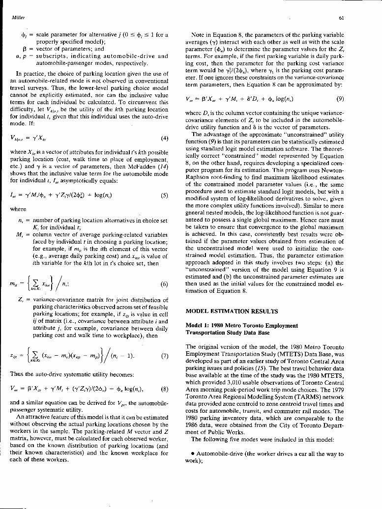
Miller

<f>j = scale parameter for alternative j (0 :s: <f>j :s: 1 for a properly specified model);

f3 = vector of parameters; and a, p = subscripts, indicating automobile-drive and

automobile-passenger modes, respectively.

In practice, the choice of parking location given the use of an automobile-related mode is not observed in conventional travel surveys. Thus, the lower-level parking choice model cannot be explicitly estimated, nor can the inclusive value terms for each individual be calculated. To circumvent this difficulty' let vkla,t be the utility of the kth parking location for individual t, given that this individual uses the auto-drive mode. If:

(4)

where Xk1 is a vector of attributes for individual t's kth possible parking location (cost, walk time to place of employment, etc.) and 'Y is a vector of parameters, then McFadden (14) shows that the inclusive value term for the automobile mode for individual t, Iar asymptotically equals:

(5)

where

n1 = number of parking location alternatives in choice set K 1 for individual t;

M 1 = column vector of average parking-related variables faced by individual tin choosing a parking location; for example, if mj1 is the ith element of this vector (e.g., average daily parking cost) and xkir is value of ith variable for the kth lot in t's choice set, then

(6)

Z 1 = variance-covariance matrix for joint distribution of parking characteristics observed across set of feasible parking locations; for example, if zijr is value in cell ij of matrix (i.e., covariance between attribute i and attribute j, for example, covariance between daily parking cost and walk time to workplace), then

(7)

Thus the auto-drive systematic utility becomes:

and a similar equation can be derived for Vpn the automobile­passenger systematic utility.

An attractive feature of this model is that it can be estimated without observing the actual parking locations chosen by the workers in the sample. The parking-related M vector and Z matrix, however, must be calculated for each observed worker, based on the known distribution of parking locations (and their known characteristics) and the known workplace for each of these workers.

61

Note in Equation 8, the parameters of the parking variable averages ( 'Y) interact with each other as well as with the scale parameter (<Va) to determine the parameter values for the Z1

terms. For example, if the first parking variable is daily park­ing cost, then the parameter for the parking cost variance term would be -yi/(2<f>a), where 'Yi is the parking cost param­eter. If one ignores these constraints on the variance-covariance term parameters, then Equation 8 can be approximated by:

(9)

where D 1 is the column vector containing the unique variance­covariance elements of Z 1 to be included in the automobile­drive utility function and B is the vector of parameters.

The advantage of the approximate "unconstrained" utility function (9) is that its parameters can be statistically estimated using standard logit model estimation software. The theoret­ically correct "constrained" model represented by Equation 8, on the other hand, requires developing a specialized com­puter program for its estimation. This program uses Newton­Raphson root-finding to find maximum likelihood estimates of the constrained model parameter values (i.e., the same procedure used to estimate standard logit models, but with a modified system of log-likelihood derivatives to solve, given the more complex utility functions involved). Similar to more general nested models, the log-likelihood function is not guar­anteed to possess a single global maximum. Hence care must be taken to ensure that convergence to the global maximum is achieved. In this case, consistently best results were ob­tained if the parameter values obtained from estimation of the unconstrained model were used to initialize the con­strained model estimation. Thus, the parameter estimation approach adopted in this study involves two steps: (a) the "unconstrained" version of the model using Equation 9 is estimated and (b) the unconstrained parameter estimates are then used as the initial values for the constrained model es­timation of Equation 8.

MODEL ESTIMATION RESULTS

Model 1: 1980 Metro Toronto Employment Transportation Study Data Base

The original version of the model, the 1980 Metro Toronto Employment Transportation Study (MTETS) Data Base, was developed as part of an earlier study of Toronto Central Area parking issues and policies (15). The best travel behavior data base available at the time of the study was the 1980 MTETS, which provided 3,010 usable observations of Toronto Central Area morning peak-period work trip mode choices. The 1979 Toronto Area Regional Modelling System (T ARMS) network data provided zone centroid to zone centroid travel times and costs for automobile, transit, and commuter rail modes. The 1980 parking inventory data, which are comparable to the 1986 data, were obtained from the City of Toronto Depart­ment of Public Works.

The following five modes were included in this model:

•Automobile-drive (the worker drives a car all the way to work);

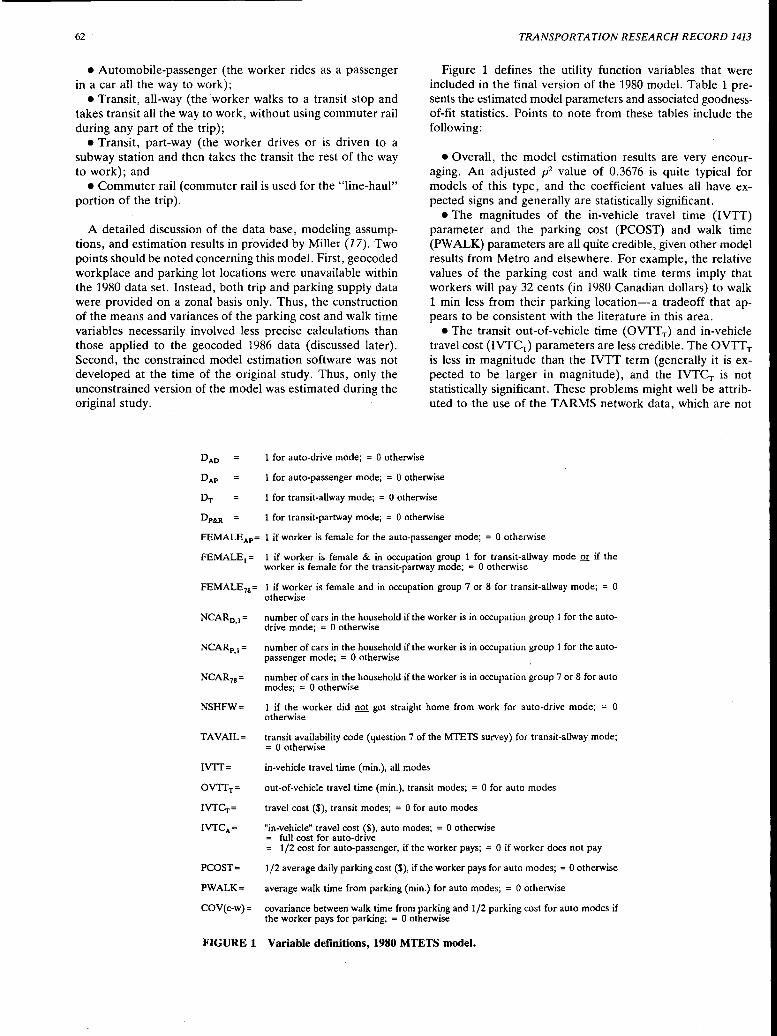
62 TRANSPORTATION RESEARCH RECORD 1413

•Automobile-passenger (the worker rides as a passenger in a car all the way to work);

Figure 1 defines the utility function variables that were included in the final version of the 1980 model. Table 1 pre­sents the estimated model parameters and associated goodness­of-fit statistics. Points to note from these tables include the following:

•Transit, all-way (the ·worker walks to a transit stop and takes transit all the way to work, without using commuter rail during any part of the trip);

•Transit, part-way (the worker drives or is driven to a subway station and then takes the transit the rest of the way to work); and

• Commuter rail (commuter rail is used for the "line-haul" portion of the trip).

A detailed discussion of the data base, modeling assump­tions, and estimation results in provided by Miller (17). Two points should be noted concerning this model. First, geocoded workplace and parking lot locations were unavailable within the 1980 data set. Instead, both trip and parking supply data were provided on a zonal basis only. Thus, the construction of the means and variances of the parking cost and walk time variables necessarily involved less precise calculations than those applied to the geocoded 1986 data (discussed later). Second, the constrained model estimation software was not developed at the time of the original study. Thus, only the unconstrained version of the model was estimated during the original study.

DAD 1 for auto-drive mode; = 0 otherwise

•Overall, the model estimation results are very encour­aging. An adjusted p2 value of 0.3676 is quite typical for models of this type, and the coefficient values all have ex­pected signs and generally are statistically significant.

• The magnitudes of the in-vehicle travel time (IVTT) parameter and the parking cost (PCOST) and walk time (PW ALK) parameters are all quite credible, given other model results from Metro and elsewhere. For example, the relative values of the parking cost and walk time terms imply that workers will pay 32 cents (in 1980 Canadian dollars) to walk 1 min less from their parking location-a tradeoff that ap­pears to be consistent with the literature in this area.

•The transit out-of-vehicle time (OVTTT) and in-vehicle travel cost (IVT~) parameters are less credible. The OVTTT is less in magnitude than the IVTT term (generally it is ex­pected to be larger in magnitude), and the IVT~ is not statistically significant. These problems might well be attrib­uted to the use of the T ARMS network data, which are not

D AP 1 for auto-passenger mode; = 0 otherwise

DT 1 for transit-allway mode; = 0 otherwise

DP&R 1 for transit-partway mode; = 0 otherwise

FEMALE AP= 1 if worker is female for the auto-passenger mode; = 0 otherwise

FEMALE1= 1 if worker is female & in occupation group 1 for transit-allway mode QI if the worker is female for the transit-partway mode; = 0 otherwise

FEMALE78 = 1 if worker is female and in occupation group 7 or 8 for transit-allway mode; = 0 otherwise

NCAR0 ,1=

NCARp, 1=

NCAR78 =

NSHFW=

TAVAIL=

IVTT=

OVTTT=

IVT~=

IVTCA=

PCOST=

PWALK=

COV(c-w)=

number of cars in the household if the worker is in occupation group 1 for the auto­drive mode; = 0 otherwise

number of cars in the household if the worker is in occupation group 1 for the auto­passenger mode; = 0 otherwise

number of cars in the household if the worker is in occupation group 7 or 8 for auto modes; = 0 otherwise

1 if the worker did not got straight home from work for auto-drive mode; = 0 otherwise

transit availability code (question 7 of the MTETS survey) for transit-allway mode; = 0 otherwise

in-vehicle travel time (min.), all modes

out-of-vehicle travel time (min.), transit modes; = 0 for auto modes

travel cost ($), transit modes; = 0 for auto modes

"in-vehicle" travel cost ($), auto modes; = 0 otherwise = full cost for auto-drive = 1/2 cost for auto-passenger, if the worker pays; = 0 if worker does not pay

1/2 average daily parking cost ($),if the worker pays for auto modes; = 0 otherwise

average walk time from parking (min.) for auto modes; = 0 otherwise

covariance between walk time from parking and 1/2 parking cost for auto modes if the worker pays for parking; = 0 otherwise

FIGURE 1 Variable definitions, 1980 MTETS model.

Miller

TABLE 1 1980 MTETS Model Estimation Results

Variable Parameter Value T-Statistic

DAD 6.2489 8.38

DAP 4.2428 5.64

DT 1.7429 9.71

Dp&R -0.66041 -3.82

, FEMALEAP 1.511 7.52

FEMALE1 0.71469 5.73

FEMALE78 0.37055 2.33

NCAR0 ,1 0.35609 4.36

NCARP,t 0.13227 1.27

NCAR78 0.64719 8.02

NSHFW 0.98269 7.60

TAVAIL -0.62205 -9.71

IVlT -0.073697 -13.19

OVlTT -0.045695 -4.66

IVT~ -0.0040419 -0.82

IVTCA -0.41370 -6.81

PCOST -1.6449 -19.90

PWALK -0.52143 -6.48

COV(c-w) 0.57380 9.28

No. of observations 3010 Log-likelihood ratio 2802.6 Adjusted p2 0.3676 Expected percent right 58.2

very precise with respect to these variables and which also generally do not vary much in value across trip-makers within the sample.

• Because of a combination of collinearity and lack of var­iability problems, only one Z, matrix value-the parking cost and walk time covariance-could be estimated, and the <f>log(n,) term could not be included within the model. The parking cost and walk time parameter [ COV( c-w)], however, is strongly significant with the expected sign. That is, because both the PCOST and the PWALK parameters are negative, their prod­uct [and hence the COV(c-w) parameter] is positive.

• The definition of the automobile-passenger travel cost terms (one-half the IVTC and the full parking cost) is based on the empirical results in that alternative-specific parameter estimates for these two terms indicated that the automobile­passenger values were 0.5 and 1.0 times the magnitudes of the automobile-drive terms, respectively.

Model 2: 1986 TDS Data Base

The 1986 Travel Diary Survey (TDS) used to develop the second version of the model is a 1-day diary survey of 0.4 percent of the households in the Greater Toronto Area (GT A), which provides detailed trip and personal characteristics of all household members in the sample. A particularly useful feature of the data set is that all trip origins and destinations are geocoded to the mid-blockface level, thereby permitting

63

detailed spatial analysis and network level-of-service calcu­lations. Detailed information concerning every Central Area off-street parking location was obtained from the City of To­ron_to Department of Public Works and the Environment. On the basis of the street addresses provided in this data set, these parking locations were also geocoded. Combined with the geocoded worker employment location data, this p~rmit­ted very detailed calculations of parking supply and cost mean values and variance-covariance matrices faced by each worker in the sample, on the basis of an assumed maximum walking distance of 1.0 km. For further details concerning the TDS and parking data sets, as well as the calculation of the parking­related variable means and variances-covariances, see Miller (16). Automobile in-vehicle travel times were computed on the basis of a user-equilibrium assignment of observed 1986 vehicle flows to the road network within the EMME/2 net­work modeling package, while transit in- and out-of-vehicle travel times were generated using a "disaggregate" or1gin point to destination point transit assignment procedure within EMME/2 for each observed work trip.

Five modes are defined in this model:

1. Automobile-drive all-way, 2. Automobile-passenger all-way, 3. Transit all-way (automobile access to the transit system is

ignored to simplify the network level-of-service calculations), 4. Commuter rail (all commuter rail users are assumed to

use the automobile mode to access the system, again to sim­plify level-of-service calculations), and

5. Walk all-way.

Figure 2 defines the set of variables included in the final version of the 1986 model. Table 2 presents both the uncon­strained and constrained estimation results for tiµs final model. Points to note from this table include the following:

• All coefficient estimates have the correct sign and plau­sible magnitudes.

• All coefficients are statistically significant at the 95 per­cent confidence level or better, except for a few minor vari­ables, such as LSDUM and JBS234. Note that !-statistics for the constrained model were not generated by the estimation program because of numerical matrix inversion problems as­sociated with this particular model. Experience with other model runs, however, indicates that the !-statistics will not be significantly different from those for the unconstrained model.

• Both models exhibit very good goodness-of-fit statistics, which compare favorably with the 1980 model fit statistics reported in Table 1.

•With the exception of the alternative-specific constants, the parameters of the "non-parking" variables tend to be quite stable in value from one model version to another. This is an encouraging result, in that it indicates a considerable degree of independence between the two types of variables as well as a desirable robustness in model specification.

• Moving from the unconstrained to the constrained version of the model has the following impacts:

- The non-automobile alternative-specific constants typ­ically become considerably more positive in value. This reflects the positive shift in the average automobile utility function introduced by the introduction of the parking cost

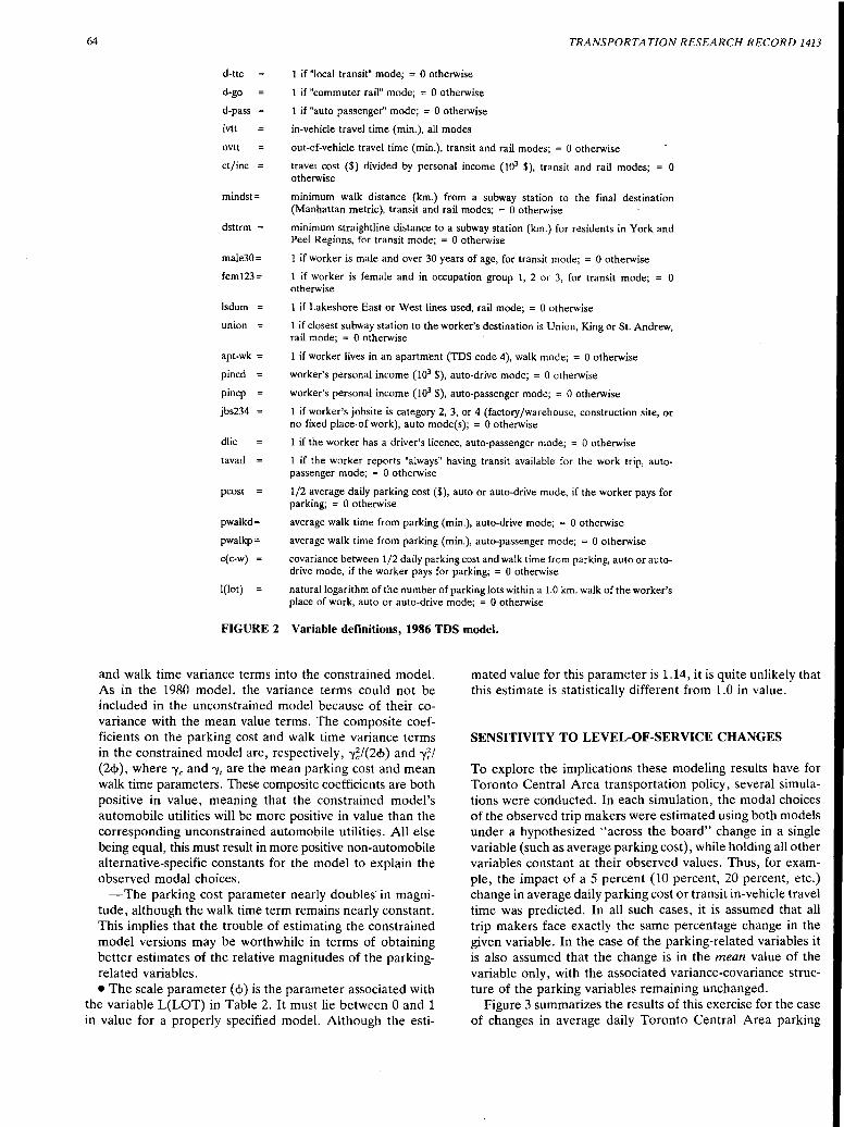
64

d-ttc

d-go

d-pass

ivtt

ovtt

ct/inc

mindst=

dsttrm =

male30=

fem123=

lsdum

union

apt-wk =

pined

pincp

jbs234

dlic

tavail

pcost =

pwalkd=

pwalkp=

c(c-w)

l(lot)

1 if "local transit" mode; = 0 otherwise

1 if "commuter rail" mode; = 0 otherwise

1 if "auto passenger" mode; = 0 otherwise

in-vehicle travel time (min.), all modes

TRANSPORTATION RESEARCH RECORD 1413

out-of-vehicle travel time (min.), transit and rail modes; = 0 otherwise

travel cost ($) divided by personal income ( 103 $), transit and rail modes; = O otherwise

minimum walk distance (km.) from a subway station to the final destination (Manhattan metric), transit and rail modes; = O otherwise

minimum straightline distance to a subway station (km.) for residents in York and Peel Regions, for transit mode; = 0 otherwise

1 if worker is male and over 30 years of age, for transit mode; = 0 otherwise

1 if worker is female and in occupation group 1, 2 or 3, for transit mode; 0 otherwise

1 if Lakeshore East or West lines used, rail mode; = 0 otherwise

1 if closest subway station to the worker's destination is Union, King or St. Andrew, rail mode; = 0 otherwise

1 if worker lives in an apartment (TDS code 4), walk mode; = 0 otherwise

worker's personal income (103 $), auto-drive mode; = 0 otherwise

worker's personal income (103 $), auto-passenger mode; = 0 otherwise

1 if worker's jobsite is category 2, 3, or 4 (factory /warehouse, construction site, or no fixed place· of work), auto mode(s); = 0 otherwise

1 if the worker has a driver's licence, auto-passenger mode; = 0 otherwise

1 if the worker reports "always" having transit available for the work trip, auto­passenger mode; = 0 otherwise

1/2 average daily parking cost ($), auto or auto-drive mode, if the worker pays for parking; = 0 otherwise

average walk time from parking (min.), auto-drive mode; = 0 otherwise

average walk time from parking (min.), auto-passenger mode; = 0 otherwise

covariance between 1/2 daily parking cost and walk time from parking, auto or auto­drive mode, if the worker pays for parking; = 0 otherwise

natural logarithm of the number of parking lots within a 1.0 km. walk of the worker's place of work, auto or auto-drive mode; = 0 otherwise

FIGURE 2 Variable definitions, 1986 TDS model.

and walk time variance terms into the constrained model. As in the 1980 model, the variance terms could not be included in the unconstrained model because of their co­variance with the mean value terms. The composite coef­ficients on the parking cost and walk time variance terms in the constrained model are, respectively, -y~/(2<!>) and -y~/ (2<!>), where 'Ye and 'Yr are the mean parking cost and mean walk time parameters. These composite coefficients are both positive in value, meaning that the constrained model's automobile utilities will be more positive in value than the corresponding unconstrained automobile utilities. All else being equal, this must result in more positive non-automobile alternative-specific constants for the model to explain the observed modal choices.

mated value for this parameter is 1.14, it is quite unlikely that this estimate is statistically different from 1.0 in value.

SENSITIVITY TO LEVEL-OF-SERVICE CHANGES

- The parking cost parameter nearly doubles' in magni­tude, although the walk time term remains nearly constant. This implies that the trouble of estimating the constrained model versions may be worthwhile in terms of obtaining better estimates of the relative magnitudes of the parking­related variables. • The scale parameter ( <!>) is the parameter associated with

the variable L(LOT) in Table 2. It must lie between 0 and 1 in value for a properly specified model. Although the esti-

To explore the implications these modeling results have for Toronto Central Area transportation policy, several simula­tions were conducted. In each simulation, the modal choices of the observed trip makers were estimated using both models under a hypothesized "across the board" change in a single variable (such as average parking cost), while holding all other variables constant at their observed values. Thus, for exam­ple, the impact of a 5 percent (10 percent, 20 percent, etc.) change in average daily parking cost or transit in-vehicle travel time was predicted. In all such cases, it is assumed that all trip makers face exactly the same percentage change in the given variable. In the case of the parking-related variables it is also assumed that the change is in the mean value of the variable only, with the associated variance-covariance struc­ture of the parking variables remaining unchanged.

Figure 3 summarizes the results of this exercise for the case of changes in average daily Toronto Central Area parking

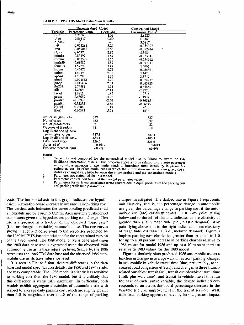
Miller

TABLE 2 1986 TDS Model Estimation Results

Unconstrained Model Variable Parameter Value T-Statistic

d-ttc d-go d-pass ivtt ovtt ct/inc mindst dsttrm male30 fem123 lsdum union apt-wk pined pincp jbs234 dlic tavail pcost pwalkd pwalkp c(c-w) l(lot)

1.7256 1.38 -0.86817 -0.59

No. of weighted obs. No. of cases

__ 2

-0.054281 -0.089042 -8.6637 -0.85197 -0.052535 -0.61982 1.5729 0.46676 1.4319 2.2829 0.021553 0.045406 0.79884

-1.2809 1.0811

-0.68057 -0.35335 -0.353353

0.22866 0.90383

No. of parameters Degrees of freedom Log-likelihood @ zero

parameter values Log-likelihood @ conv. Likelihood ratio Adjusted p2

Expected percent right

337 632 21

611

-347.1 -184.1 326.0

0.4517 68.9%

-3.21 -2.58 -2.85 -1.64 -1.55 -1.57 3.42 0.75 2.38 1.87 1.70 2.54 1.51

-2.11 1.89

-4.22 -2.56 -2.56 1.17 5.01

Constrained Model Parameter Value1

2.8225 0.14610 3.0817

-0.054307 -0.092474 -8.3984 -0.92304 -0.054302 -0.69711 1.6061 0.45430 1.4428 3.3719 0.024237 0.043323 0.64856

-1.3770 1.0716

-1.1937 -0.36515 -0.56945 __ 4

1.1436

337 632

22 610

-347. l -186.3 321.6

0.4443 69.4%

65

Notes: 1.

2. 3. 4.

T-statistics not computed for the constrained model due to failure to invert the log­likelihood info~mati<;>n ~atrix. This problem appears to be related to the auto passenger mo.de, whose mclus10n m the model tends to introduce some instability in parameter estunates, etc. In other model runs in which the information matrix was inverted the t­statistics changed very little between the unconstrained and the constrained model~. Parameter not estimated for this model. Parameter constrained to equal the pwalkd parameter value. Paramet~rs for var~ance-covariance terms constrained to equal products of the parking cost and parking walk time parameters.

costs. The horizontal axis in this graph indicates the hypoth­esized across-the-board increase in average daily parking cost. The vertical axis indicates the corresponding predicted total automobile use by Toronto Central Area morning peak-period commuters given the hypothesized parking cost change. This use is expressed as a fraction of the observed "base case" (i.e., no change in variable) automobile use. The two curves shown in Figure 3 correspond to the responses predicted by the 1980 MTETS-based model and for the constrained version of the 1986 model. The 1980 model curve is generated using the 1980 data base and is expressed using the observed 1980 automobile use as its base reference level. Similarly, the 1986 curve uses the 1986 TDS data base and the observed 1986 auto­mobile use as its base reference level.

It is seen in Figure 3 that, despite differences in the data base and model specification details, the 1980 and 1986 results are very comparable. The 1986 model is slightly less sensitive to parking cost than the 1980 model, but it is unlikely that this difference is statistically significant. In particular, both models exhibit aggregate elasticities of automobile use with respect to average daily parking cost, which are slightly greater than 1.0 in magnitude over much of the range of parking

charges investigated. The dashed line in Figure 3 represents unit elasticity, that is, the percentage change in automobile use given the percentage change in parking cost if the auto­mobile use (arc) elasticity equals -1.0. Any point falling below and to the left of this line indicates an arc elasticity of greater than 1.0 in magnitude (i.e., elastic demand). Any point lying above and to the right indicates an arc elasticity of magnitude less than 1.0 (i.e., inelastic demand). Figure 3 implies parking cost elasticities greater than or equal to 1.0 for up to a 30 percent increase in parking charges relative to 1986 values for model 1986 and up to a 40 percent increase relative to 1980 values for the 1980 model.

Figure 4 similarly plots predicted 1986 automobile use as a function in changes in average walk times from parking, changes in automobile in-vehicle travel time (due, presumably, to in­creased road congestion effects), and changes in three transit­related variables: transit fare, transit out-of-vehicle travel time (walk plus wait time), and transit in-vehicle travel time. In the case of each transit variable, the change indicated cor­responds to an across-the-board percentage decrease in the variable (i.e., an improvement in the transit service). Walk time from parking appears to have by far the greatest impact

FRACTION OF BASE AUTO USAGE

0.90 ...----- UNIT ELASTICITY LINE ~ ~

'"'-0.80

0.70

0.60

0.50

0.40

0.30

10 20 30 40 % CHANGE IN AVERAGE DAILY PARKING COST

FIGURE 3 Predicted changes in Toronto Central Area automobile use given changes in average daily parking cost.

so

FRACTION OF BASE AUTO USAGE

0.90

0.80

0.70

0.60

0.50

0.40

0.30

ALL CURVES ARE FOR 1986 MODEL.

TRANSIT CHANGES ARE DECREASES.

AUTO CHANGES ARE INCREASES.

10 20 30 40 % CHANGE IN SERVICE VARIABLE

TRANSIT FARE

so

TRANSIT OUf-OF­VEH. TIME

TRANSIT IN-VEii. TIME

AUlO NVEH. 1lME

PARKING COST

PARKING WALK TIME

FIGURE 4 Predicted Changes in Toronto Central Area automobile use given changes in selected automobile and transit service characteristics.

Miller

on automobile use, generating arc elasticities greater than 1.0 over the entire range of times examined. Parking cost and automobile in-vehicle travel time are the next most important determinants of automobile use (with automobile use being slightly inelastic over the entire range of values examined). Finally, Figure 4 illustrates that improvements in transit serv­ice levels are predicted to have less impact than corresponding percentage reductions in auto service levels on Toronto Cen-

. tral Area automobile use. As in the parking cost case, the elas­ticities obtained from the 1980 model for each of these vari­ables are very similar to the 1986 results shown in Figure 4.

Two other experiments were conducted using this model. In the first, it is assumed that free parking is eliminated for all Central Area commuters, thus requiring all commuters who drive to pay full, unsubsidized parking prices. In the second, it is assumed that a free transit pass is provided to all commuters. Figure 5 indicates the predicted impacts of each policy on automobile use, with and without associated changes in average parking price, and compares these impacts with the status quo case (i.e., no free pass, free parking for some). Note that the vertical axis in this case is the actual automobile-drive mode split.

As indicated by Figure 5, providing free transit passes to all Central Area commuters is predicted to reduce automobile­drive use from the base case of 20 percent to 16.9 percent. Elimination of free parking for commuters is predicted to yield an even greater reduction in automobile drivers to 15.8 per­cent. These reductions are comparable in their impacts to increase in average Central Area parking prices of 23.5 per­cent and 32.5 percent under status quo conditions. If increased

% OF WORKERS USING AUTO-DRIVE MODE 20

67

parking charges are implemented in combination with one of these two policies, the net impact is, of course, greater.

The preceding policies are very abstract in nature (e.g., increase average daily parking cost by 25 percent). The model, however, can be readily extended to more realistic policy analyses as well as incorporated within a more generalized modeling framework. Points to note in this regard include the following:

• Because parking location utility function parameters ( -y) are estimated within the model, the lower-level parking lo­cation choice model (Equation 2) can be reconstructed from the results presented here and used to predict explicitly park­ing location choices, given known employment distributions and automobile use levels (as defined by Equation 1). This model could be used to determine parking market potentials at various points, compute spatially distributed parking price elasticities, combine with a parking supply model to model parking market interactions, and accomplish other objectives as well.

• Without engaging in full supply-demand modeling of the parking market, more realistic parking policies could be an­alyzed by changing the spatial price/supply distributions on a scenario basis (e.g., eliminate all parking within x meters of subway stations; increase parking prices only within the Cen­tral Business District).

•Walk times from parking locations to employment sites were computed within this analysis on a simple rectilinear or "Manhattan" basis (which, given the dense grid street layout within the Central Area, undoubtedly represents a close ap-

18 (

23.5% CHANGE IN PARKING COST YIELDS SAME IMPACT AS FREE TRANSIT PASSES

32.5% CHANGE IN PARKING COST YIELDS SAME IMPACT

16

14

12

10

8

6

ALL CURVES ARE FOR THE 1986 MODEL

10

/ AS NO "FREE" PARKING

20 30 40 so % CHANGE IN DAILY PARKING CHARGE

BASE CASE

"FREE TRANSIT"

"PAY FOR PARKING"

FIGURE 5 Predicted changes in Toronto Central Area automobile use given fundamental changes in cost of parking and transit.

68

proximation to actual shortest-path walk times). If more de­tailed treatment of walk paths is required, the geocoded na­ture of the data base readily permits its incorporation within a geographic information system capable of performing such detailed calculations.

• The overall mode choice model is readily incorporated within a larger demand modeling system because it is simply a multinomial logit model with an expanded set of parking­related variables in its automobile-mode utility functions.

METHODOLOGICAL ISSUES

Although this paper primarily focuses on the empirical in­vestigation of Central Area work mode choice sensitivity to parking-policy-related variables, three points of somewhat more general methodological interest emerge from this work that should be briefly noted.

First, McFadden's (14) approximation for the inclusive value term permits theoretically sound nested logit models to be empirically estimated in the absence of explicit information concerning lower-level choices (in this example, the choice of parking location given use of the automobile for the work trip). Specifically, in cases in which heterogeneity within and covariance among the lower-level attributes exist (in this ex­ample, considerable variation exists in parking costs and walk times associated with the set of parking locations in any work­er's choice set). Typically the assumption is made that the unobserved lower-level is homogeneous (e.g., a residential location and type choice model may assume that all houses of a given type within a given zone possess identical charac­teristics). Under this assumption, the variance-covariance terms in the upper-level utility function equivalent to Equation 5 is identically zero in value, thereby considerably simplifying the analysis. The preceding, however, demonstrates that, in the presence of significant lower-level heterogeneity, this as­sumption can bias model parameter estimations.

Second, the relative transferrability of the aggregate elas­ticities of the 1980 and 1986 models is noteworthy, especially given that these models would undoubtedly fail most normal transferrability tests (similarity in parameter values, etc.). This result is reasonably similar to that recently found by Laferriere in the case of disaggregate intercity mode choice models, in which models from Canada, the United Kingdom, and the United States are found to have fairly consistent aggregate own and cross-price elasticities, despite great variations in calibration study area and base year and despite little evidence of parameter transferability (18).

Finally, problems in developing' a stable model that included the automobile-passenger mode prompted some early model estimations in which the automobile-drive and automobile­passenger modes were combined into a composite automobile mode. In addition, runs were performed in which information concerning whether or not the worker paid for parking was ignored, so that the model assumed that all workers paid for parking. In both cases, the overall utility function specification remained the same (with the obvious exception that automobile­passenger-related variables disappear in the "composite" models). Very little change occurred in parameter estimates across the three models, except in the case of the parking cost parameter, which changed from -0.220 ("composite" model,

TRANSPORTATION RESEARCH RECORD 1413

no allowance for free parking) to -0.706 ("composite" model, free parking accounted for) to -1.194 (separate drive and passenger modes plus free parking). Figure 6 summarizes the impacts these assumptions have on model sensitivity to park­ing cost.

Figure 6 also illustrates the dramatic effect the improved model specification has on model sensitivity to parking cost (and, more generally, on eliminating parameter bias). The composite-automobile, no-free-parking model appears to be quite insensitive to parking cost changes. Introducing the free parking effect significantly increases the model sensitivity. Introduction of explicit representation of automobik passen­gers (who are likely to be less sensitive to parking costs than automobile drivers) further improves the model sensitivity.

This result may seem trivially self-evident: obviously im­proving model specification will yield improved model results. In the development of practical, operational planning models, however, considerable pressure exists to simplify model spec­ification so as to simplify the forecasting problem. The net result, as indicated by Figure 6, is often a model that possesses biased coefficients and hence is much less useful as a fore­casting and policy analysis tool. Further, such biases are typ­ically difficult if not impossible to identify within the model development and application process. This is primarily be­cause more general model specifications (which provide an analytical and statistical framework for testing the simplifying assumptions) are simply not considered.

SUMMARY

This paper has presented a disaggregate model of central area work trip mode choice that incorporates a detailed treatment of parking supply and cost impacts. Two versions of this model are presented: one estimated using 1980 travel survey data and one based on more recent 1986 data. The results obtained from the two models are very consistent in terms of the ag­gregate elasticities displayed with respect to walk time from parking, parking cost, and other automobile- and transit-related variables. The models indicate that central area commuters are very sensitive to changes in parking walk times and park­ing cost, somewhat less sensitive to automobile and transit in-vehicle travel times (in order of decreasing sensitivity) and less sensitive again to changes in transit out-of-vehicle travel time and fare. Additional, more detailed survey information concerning automobile-driver attitudes, reasons for auto­mobile use, and other related information, however, would be very useful in providing additional insight into the role of parking in determining central area work trip mode choice.

ACKNOWLEDGMENTS

This study was funded by the City of Toronto Planning and Development Department. Special thanks are due to Greg Stewart of the Planning Department, without whose support this project would not have been possible. The comments of Norris Zucchet and Ian Maher of the City of Toronto Parking Authority and John Mende of the City of Toronto Depart­ment of Public Works and the Environment are also appre­ciated. Parking data were provided by the Department of

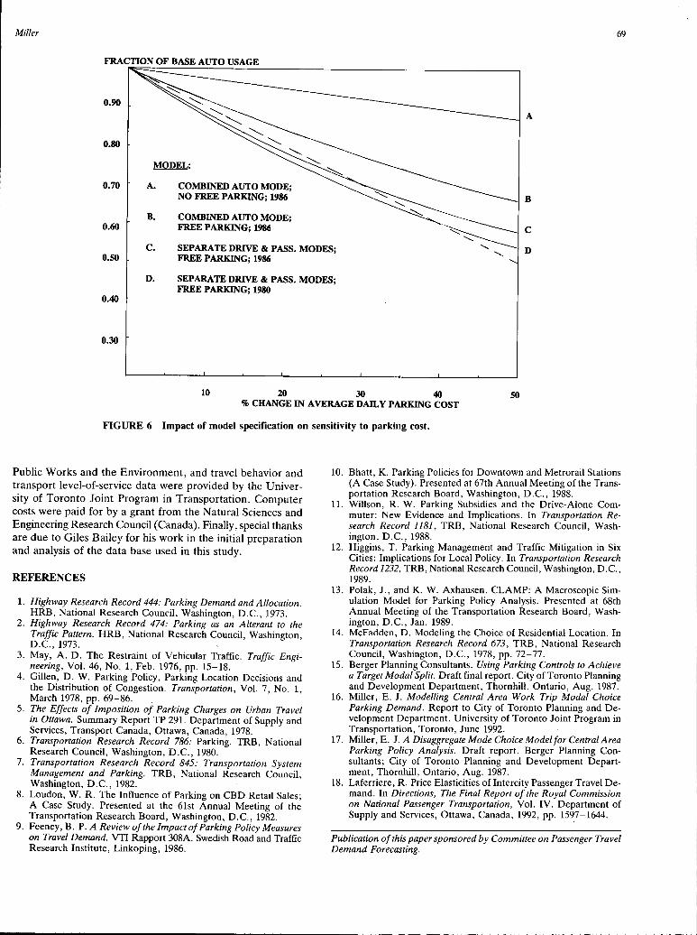
Miller 69

A

B

c

D

0.30

10 20 30 40 so % CHANGE IN AVERAGE DAILY PARKING COST

FIGURE 6 Impact of model specification on sensitivity to parking cost.

Public Works and the Environment, and travel behavior and transport level-of-service data were provided by the Univer­sity of Toronto Joint Program in Transportation. Computer costs were paid for by a grant from the Natural Sciences and Engineering Research Council (Canada). Finally, special thanks are due to Giles Bailey for his work in the initial preparation and analysis of the data base used in this study.

REFERENCES

1. Highway Research Record 444: Parking Demand and Allocation. HRB, National Research Council, Washington, D.C., 1973.

2. Highway Research Record 474: Parking as an Alterant to the Traffic Pattern. HRB, National Research Council, Washington, D.C., 1973. .

3. May, A. D. The Restraint of Vehicular Traffic. Traffic Engi­neering, Vol. 46, No. 1, Feb. 1976, pp. 15-18.

4. Gillen, D. W. Parking Policy, Parking Location Decisions and the Distribution of Congestion. Transportation, Vol. 7, No. 1, March 1978, pp. 69-86. .

5. The Effects of Imposition of Parking Charges on Urban Travel in Ottawa. Summary Report TP 291. Department of Supply and Services, Transport Canada, Ottawa, Canada, 1978.

6. Transportation Research Record 786: Parking. TRB, National Research Council, Washington, D.C., 1980.

7. Transportation Research Record 845: Transportation System Mana~ement and Parking. TRB, National Research Council, Washmgton, D.C., 1982.

8. Loudon, W. R. The Influence of Parking on CBD Retail Sales; A Case Study. Presented at the 61st Annual Meeting of the Transportation Research Board, Washington, D.C., 1982.

9. Feeney, B. P. A Review of the Impact of Parking Policy Measures on Travel Demand. VTI Rapport 308A. Swedish Road and Traffic Research Institute, Linkoping, 1986.

10. Bhatt, K. Parking Policies for Downtown and Metrorail Stations (A Case Study). Presented at 67th Annual Meeting of the Trans­portation Research Board, Washington, D.C., 1988.

11. Willson, R. W. Parking Subsidies and the Drive-Alone Com­muter: New Evidence and Implications. In Transportation Re­search Record 1181, TRB, National Research Council, Wash­ington, D.C., 1988.

12. Higgins, T. Parking Management and Traffic Mitigation in Six Cities: Implications for Local Policy. In Transportation Research Record 1232, TRB, National Research Council, Washington, D.C., 1989.

13. Polak, J., and K. W. Axhausen. CLAMP: A Macroscopic Sim­ulation Model for Parking Policy Analysis. Presented at 68th Annual Meeting of the Transportation Research Board, Wash­ington, D.C., Jan. 1989.

14. McFadden, D. Modeling the Choice of Residential Location. In Transportation Research Record 673, TRB, National Research Council, Washington, D.C., 1978, pp. 72-77.

15. Berger Planning Consultants. Using Parking Controls to Achieve a Target Modal Split. Draft final report. City of Toronto Planning and Development Department, Thornhill, Ontario, Aug. 1987.

16. Miller, E. J. Modelling Central Area Work Trip Modal Choice Parking Demand. Report to City of Toronto Planning and De­velopment Department. University of Toronto Joint Program in Transportation, Toronto, June 1992.

17. Miller, E. J. A Disaggregate Mode Choice Mode/for Central Area Parking Policy Analysis. Draft report. Berger Planning Con­sultants; City of Toronto Planning and Development Depart­ment, Thornhill, Ontario, Aug. 1987.

18. Laferriere, R. Price Elasticities of Intercity Passenger Travel De­mand. In Directions, The Final Report of the Royal Commission on National Passenger Transportation, Vol. IV. Department of Supply and Services, Ottawa, Canada, 1992, pp. 1597-1644.

Publication of this paper sponsored by Committee on Passenger Travel Demand Forecasting.

70 TRANSPORTATION RESEARCH RECORD 1413

Integrating Feedback into Transportation Planning Model: Structure and Application

DAVID LEVINSON AND AJAY KUMAR

A new structure for the transportation planning model that in­cludes feedback among demand, assignment, and traffic control is presented. New methods, combined with a renewed interest in transportation planning models prompted by the Clean Air Act of 1990 and the Intermodal Surface Transportation Efficiency Act of 1991, warrant reconsideration of the traditional four-step trans­portation planning model. An algorithm for feedback that results in consistent travel times as input to travel demand and output from route assignment is presented. The model, including six stages of Trip Generation, Destination Choice, Mode Choice, Departure Time Choice, Route Assignment, and Intersection Control, is briefly outlined. This is followed by an application comparing a base year 1990 application with a forecast year of 2010. The 2010 forecast is solved both with and without feedback for comparison purposes. Incorporation of feedback gives sig­nificantly different results than does the standard model.

Conventionally applied transportation planning models con­forming to the Urban Transportation Modeling System (UTMS) have four sequential steps of trip generation, trip distribution,. mode choice, and route assignment (J). Available evidence suggests that UTMS is not a behavioral representation of trip making. Foremost, when the four-step model is strictly ap­plied, there is no feedback between the travel time on the network and the estimation of demand. It is widely under­stood that if congestion is significant, it will affect the indi­vidual's decision to make the trip, choice of destination, mode, and departure time. Moreover, this model structure does not account for the impact of signal control on route choice and travel demand. For many trips, delay at intersections is as significant as vehicle running time, and a prolonged delay may motivate a change in route. Not incorporating elastic demand or responsive intersection control in the theoretical framework will cause an incorrect representation of network flow (2).

Over the past 20 years, methods have been developed to model the feedback among assignment, demand, and inter­section control. Recently, some literature has proposed com­bining demand, assignment, and intersection control into a sfogle modeling framework (2,3). This paper reviews the the­ory and develops a procedure with feedback among assign­ment, demand, and intersection control. The procedure is applied to the Baltimore-Washington metropolitan region. The results suggest that introducing feedback between con­gested travel times and demand and between link flows and intersection control provides a more realistic representation of travel patterns and traffic flows. The procedure is especially relevant in the context of long-term forecasting where the

Montgomery County Planning Department, 8787 Georgia Avenue, Silver Spring, Md. 20910.

possible interrelationship between travel demand and emerg­ing metropolitan structure is less understood.

RESEARCH

It has long been recognized that travel demand is influenced by network supply. The example of a new bridge opening where none was before, inducing additional traffic, has been noted for centuries. Much research has gone into developing methods for allowing the forecasting system to directly ac­count for this phenomenon. Evans published her doctoral dissertation on a mathematically rigorous combination of the gravity distribution model with the equilibrium assignment model ( 4). The earliest citation of this integration is the work of Irwin and Von Cube, as related by Florian et al., who comment on the work of Evans:

The work of Evans resembles somewhat the algorithms devel­oped by Irwin and Von Cube [Bulletin 347: Capacity Restraint in Multi-Travel Mode Assignment Programs, HRB, 1962] for a transportation study of Toronto, Canada. Their work allows for feedback between congested assignment and trip distribution, although they apply sequential procedures. Starting from an ini­tial solution of the distribution problem, the interzonal trips are assigned to the initial shortest routes. For successive iterations, new shortest routes are computed, and their lengths are used as access times for input the distribution model. The new interzonal flows are then assigned in some proportion to the routes already found. The procedure is stopped when the interzonal times for successive iteration are quasi-equal. (5)

Florian et al. proposed a somewhat different method for solv­ing the combined distribution assignment, applying the Frank­Wolfe algorithm directly. Boyce et al. provide an excellent summary of the research to date on network equilibrium prob­lems, including the assignment with elastic demand (6).

Signal-setting policies generally assume that route choices are unaffected by the signal settings chosen (7). The reverse is also held true, signal settings are unaffected by the routes chosen. This presumption of independence results in a lag in change to signal policies, which reaffirm themselves in more static traffic patterns. The assumption of complete independ­ence is not supported by available evidence. Common ex­perience suggests that signal policies that provide faster travel on arterials than side streets help to induce drivers to use the favored roads. Moreover, considering the relationship will be even more critical in projecting traffic trends. Over time, signal policies do respond to changes in travel demand.

To overcome these problems, several attempts have been made to combine an assignment algorithm with intersection control. These have generally been developed to improve

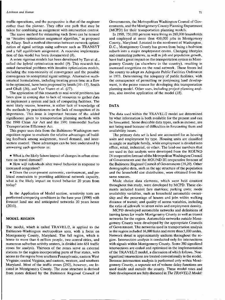
Levinson and Kumar

traffic operations, and the perspective is that of the engineer rather than the planner. They offer one path that may be taken for combining as assignment with intersection control.

The naive method for estimating such flows can be termed an "iterative optimization assignment algorithm," as proposed by Allsop. Such a method alternates between network optimi­zation of signal settings using software such as TRANSIT and a full equilibrium assignment. A recursive implementa­tion of this model has been documented (8).

A more rigorous models has been developed by Tan et al., called the hybrid optimization model (9). This research has noted theoretical problems with iterative optimization models, including the non-necessity of convergence and the possible convergence to nonoptimal signal settings. Alternative math­ematical formulations, including treating green time as a flow to be optimized, have been proposed by Smith (10-15), Smith and Ghali (16), and Van Vuren et al. (17).

The application of this research to real-world problems has been slow in coming due to lack of resources to gather data or implement a system and lack of computing facilities. The most likely reason, however, is either lack of knowledge of the methods by practitioners or the lack of recognition of its importance. This issue is important because of the added significance given to transportation planning methods with the 1990 Clean Air Act and the 1991 lntermodal Surface Transportation Efficiency Act.

This paper uses data from the Baltimore-Washington met­ropolitan region to evaluate the relative advantages of build­ing feedback among assignment, travel demand, and inter­section control. These advantages can be best understood by answering such questions as:

• What is the likely future impact of changes in urban struc­ture on travel demand?

• How will individuals alter travel behavior in response to increased congestion?

• Given the ever-present economic, environment, and po­litical constraints to providing additional network capacity, what is the likely impact on travel behavior 20 years from today?

In the Application of Model section, sensitivity tests are performed comparing conditions in the base year (1990) with forecast land use and anticipated networks 20 years hence (2010).

MODEL REGION

The model, which is called TRAVEL/2, is applied to the Baltimore-Washington metropolitan area, with a focus on Montgomery County, Maryland. The full region, which is home to more than 6 million people, two central cities, and numerous suburban activity centers, is divided into 651 traffic zones for analysis. Thirteen of the zones serve as external stations to the region incorporating parts of four states, with access to the region from southern Pennsylvania; eastern West Virginia; central Virginia; and eastern, western, and southern Maryland. Most of the traffic zones (292), however, are lo­cated in Montgomery County. The zone structure is derived from zones defined by the Baltimore Regional Council of

71

Governments, the Metropolitan Washington Council of Gov­ernments, and the Montgomery County Planning Department (MCPD) for their transportation planning models.

In 1990, 750,000 persons were living in 280,000 households and employed at more than 410,000 jobs in Montgomery County, Maryland. Located to the northwest of Washington, D.C., Montgomery County has grown from being a bedroom suburb into a major employment center. Changing lifestyles and commuting patterns, as well as job and population growth, have had a great impact on the transportation system in Mont­gomery County (as elsewhere in the country), resulting in increased congestion on the road network. These forces led the county to adopt an Adequate Public Facilities Ordinance in 1973. Determining the adequacy of public facilities, with the consequence of permitting or postponing land develop­ment, is the prime reason for developing this transportation planning model. Other uses, including project planning an~l­ysis, also involve application of the model (18).

DATA

The data used within the TRA VEL/2 model are determined by what information is both available for the present and can be forecasted. Some desirable data types, such as income, are not being used because of difficulties in forecasting them and availability issues.

The primary data set is land use accounted for as housing units and employment by type. Housing units are classified as single or multiple family, while employment is divided into office, retail, industrial, or other. The land-use numbers that are used in this analysis were developed from the ROUND IV cooperative forecast of the Metropolitan Washington Council of Governments and the ROUND III cooperative forecast of the Baltimore Regional Council of Governments (19,20). Other demographic data, such as the age structure of the population and the household size distribution, were obtained from the same sources.

Mode choice data elements, which were held constant throughout this study, were developed by MCPD. These ele­ments included transit fare matrices; parking costs; mode availability variables, such as household automobile owner­ship and the percentage of houses and jobs within walking distance of transit; and quality of access variables, including the ratio of sidewalk to street miles and employment density.

MCPD developed automobile networks and definitions of turning lanes for inside Montgomery County as well as transit networks for the region. Automobile networks outside Mont­gomery County were developed by the appropriate Councils of Government. The networks used in transportation analysis in the region included 16,000 links and more than 5,000 nodes. Network detail is approximately uniform throughout the re­gion. Intersection analysis is conducted only for intersections with signals within Montgomery County. Some 380 signalized intersections are coded and optimized in the implementation of the TRA VEL/2 model, a discussion of which follows. Non­signalized intersections are treated conventionally in the model. Because intersection analysis is performed only within Mont­gomery County, a separate set of volume delay functions are used inside and outside the county. These model rates and their development are fully discussed in The TRA VEL/2 Model:

72

Technical Documentation (21). The data sources are discussed in The TRAVEL/2 Model & Transportation Information Sys­tem User's Guide (22).

MODEL STRUCTURE

The TRA VEL/2 model structure differs from the conven­tional model in several ways. Figure 1 shows a flowchart of this model structure, which can be compared with the con­ventional transportation planning model shown in Figure 2. The algorithm to execute assignment with intersection control and elastic demand is shown in Figure 3. The TRA VEL/2 model is set up for internal feedback so that when an elastic­demand assignment is performed, the travel times input to the demand become identical to those output from the as­signment when the model converges to a solution. This model also contains responsive intersection control, which in the conventional model is implicitly static and nonresponsive. Further, the model explicitly contains a stage where departure time choice is considered as a function of congestion variables.

MODEL COMPONENTS

Numerous equations, functions, and mathematical relation­ships comprise the TRA VEL/2 model. Specifying them all is beyond the scope of this section, as noted before. They are provided in the Round IV Cooperative Forecast for the Bal­timore area (21). However, the basic variables and structures are discussed below.

Trip Generation

Trip generation has several components. Trip rates at the home end are estimated from a cross-classification model,

Trip Generation

Trip Distribution

I Route Assignment I

IJ•••I FIGURE 1 Conventional transportation planning model.

TRANSPORTATION RESEARCH RECORD 1413

where the rate applied is a function of dwelling type, house­hold size, and age of the trip maker. There are two dwelling types: single and multiple family. There are five household sizes, ranging from 1 to 5 or more persons (5 categories). The age of the trip maker is the percentage of persons in each 5-year age cohort from 0 to 85 + (18 categories). At the work end, trip rates are a function of employment by type, namely office, retail, and other employees. At the nonhome, nonwork end, trips are a function of retail employment and population. Trip rates have been .estimated for seven purposes, including specific chained work to home trips.

Trip Distribution

Trip distribution as applied uses the doubly constrained grav­ity model structure. Impedance functions have been estimated for each trip purpose. Impedance is defined as a function of congested automobile travel time. The authors worked.sep­arately to improve this model to use a composite multimodal impedance function. The following equation is used:

where

t;j = number of trips from origin i to destination j, p; = number of trips produced at origin i, qj = number of trips attracted to destination j (total trip

origins = total trip destinations), and k;j = socioeconomic adjustment factor for zone interchange

i to j = 1.

The friction factor is as follows:

where b is deterrence coefficient and cij is peak-hour travel time between origin i and destination j.

Mode Choice

Mode choice is estimated as a multinomial logit model for seven modes and two primary purposes (work and nonwork). The factors determining the utilities of mode choice are travel time, mode availability, the quality of the access trip, and cost. The actual relationships in the model use the variables relative time and relative cost, which are the ratio of the time, or cost, of a mode divided by the time, or cost, of making the same trip by driving alone in the base year 1989. The 1989 automobile time and automobile cost serve as a constant base on which to normalize the model relationships. The higher the "relative time," the less attractive the mode, which is true for both automobile and nonautomobile modes. For the base year, the automobile relative time and relative cost equal 1:

exp( Um) M

· L exp(Um) m=l

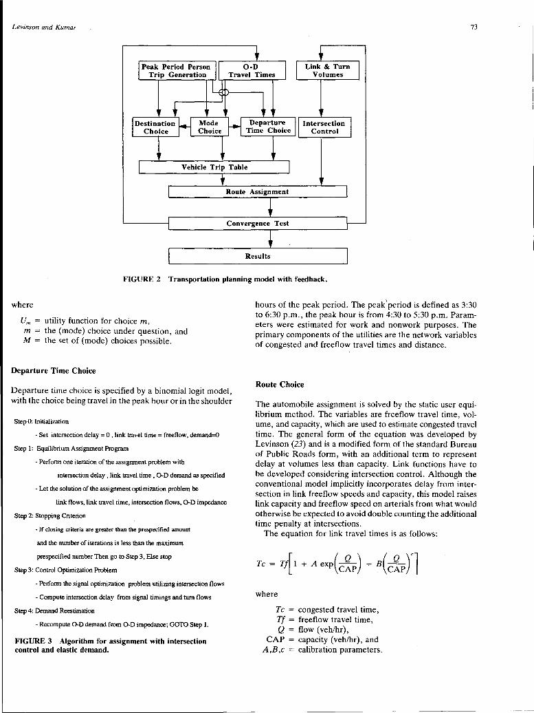
Levinson and Kumar

0-D Travel Times

Link & Turn Volumes

73

Vehicle Trip Table

Route Assignment

Convergence Test

Results

FIGURE 2 Transportation planning model with feedback.

where

um = utility function for choice m, m = the (mode) choice under question, and M = the set of (mode) choices possible.

Departure Time Choice

Departure time choice is specified by a binomial lo git model, with the choice being travel in the peak hour or in the shoulder

Step 0: Initialization

- Set intersection delay= 0, link travel time= freeflow, demand=O

Step 1: F.quilibrium Assignment Program

- Perform one iteration of the assignment problem with

intersection delay , link travel time , 0-D demand as specified

- Let the solution of the assignment optimization problem be

link flows, link travel time, intersection flows, 0-D impedance

Step 2: Stopping Criterion

- If closing criteria are greater than the prespecified amount

and the number of iterations is less than the maximum

prespecified number Then go to Step 3, Else stop

Step 3: Control Optimization Problem

- Perform the signal optimization problem utilizing intersection flows

- Compute intersection delay from signal timings and tum flows

Step 4: Demand Reestimation

- Recompute 0-D demand from 0-D impedance; GOTO Step 1.

FIGURE 3 Algorithm for assignment with intersection control and elastic demand.

hours of the peak period. The peak1period is defined as 3:30

to 6:30 p.m., the peak hour is from 4:30 to 5:30 p.m. Param­eters were estimated for work and nonwork purposes. The primary components of the utilities are the network variables of congested and freeflow travel times and distance.

Route Choice

The automobile assignment is solved by the static user equi­librium method. The variables are freeflow travel time, vol­ume, and capacity, which are used to estimate congested travel time. The general form of the equation was developed by Levinson (23) and is a modified form of the standard Bureau of Public Roads form, with an additional term to represent delay at volumes less than capacity. Link functions have to be developed considering intersection control. Although the conventional model implicitly incorporates delay from inter­section in link freeflow speeds and capacity, this model raises link capacity and freeflow speed on arterials from what would otherwise be expected to avoid double counting the additional time penalty at intersections.

The equation for link travel times is as follows:

where

Tc Tf =

Q CAP

A,B,c

congested travel time, freeflow travel time, flow (veh/hr), capacity (veh/hr), and calibration parameters.

74

Intersection Control

The output of the intersection control model is the average delay for a turning movement. The delay model is the Hurdle model (24), and cycle time and green time is estimated using methodologies suggested by Webster (25). Lane adjustment factors and lane utilization factors are adopted from Chapter 9 of the Highway Capacity Manual (26). The green time is assigned to equalize the volume/saturation flow on the critical approaches.

The equations for congested travel times at intersections are as follows:

(i - c~c) (c~P -1) d = CYC

2 + T

2

CYC = (1.5L + 5)

( l.O - pt, S~T) where

d = average delay, CYC = cycle length,

T = length of congested time period, g = green phase length, L = lost time per cycle, Q = volume (flow) on movement in vehicles per T,

CAP = capacity on movement [(g/CYC) * SAT], SAT = saturation flow rate (1,800 veh/hr of green), and

p = phase.

APPLICATION OF MODEL

This section discusses several sensitivity tests that were per­formed using the TRA VEL/2 model. The model is tested by running the model for two different time periods: a 1990 base year and a 2010 forecast year. Various results are compared for the two time frames to demonstrate how feedback affects results for a typical application.

The data sensitivity tests here compare 1990 and 2010 land use and demographics on 1990 and 2010 automobile and transit networks. Summaries of some key data (for Montgomery County) are presented in the following table:

1990 2010 Data Input (thousands) (thousands)

Housing units 280 340 Jobs 415 650 Road capacity 3,210 4,190

Mode choice was not iterated within the feedback process and therefore is not discussed. The mode choice in these runs was solved previously using congested times for both the base 1~9.0 and future 2010 scenarios. The formulation of the mode choice model, including non-automobile times, costs, and trip quality variables, makes it both relatively insensitive to changes in travel times and computationally intensive.

Trip Generation

As noted e_arlier, for the home end of trips, generation is determined with a cross-classification model, while a regres­sion model is used for the nonhome end of trips (21). In

TRANSPORTATION RESEARCH RECORD 1413

Montgomery County, for the base year 1990, Figure 4 suggests that 27 percent of all afternoon work-to-home trips originating in Montgomery County have stops, and 29 percent of those trips destined for the county are linked. Estimates of the forecast year 2010 are similar, with 28 percent of those trips being linked.

The normalization procedure results in the total number of work to other (linked) destinations, which is equal to the number of other-to-home (linked) origins at the traffic zone level. Regionally, the number of trip origins equals the num­ber of trip destinations for each purpose.

Given that these trips are significant in trip generation, they can be expected to affect distribution. Chained trips are dis­tributed as if they are two trips: work-to-other (linked) trip and other-to-home (linked) trip. Both of these trip purposes have different, and shorter, trip length distributions than work­to-home trips.

Trip generation for nonwork trips is also important. These trips grow significantly over the period with changing land use and demographics. A 21 percent increase is found in nonwork trips, which compares with a similar 18 percent in­crease in households.

Departure Time Choice

The TRA VEL/2 model includes an explicit model of depar­ture time choice as a function of congestion. Given a 3-hr peak period with a fixed number of trips, the peak hour would have no less than 33 percent of all peak period travel. Work trips, however, exceed that fraction as they are less elastic in departure time choice than nonwork trips. Nonwork trips also tend to peak in the third hour of the afternoon peak period, and work trips (and traffic overall) peak in the second hour. However, because of the greater length of work trips, more than one-third of all peak period travel occurs in the peak travel hour.

By assuming contant factors over time instead of incor­porating a congestion-based departure time choice model, the result would be 6 percent more work and 10 percent more nonwork trips on the road network in the forecast year. This quantity of trips is certainly significant, particularly consid­ering the desire to use the model in a relativistic fashion, comparing a future forecast with a base year estimate.

Destination Choice

Application of the model suggests that congestion in 2010 will be worse than the base year. Without feedback, 2010 would

500-.---.~~~.....-~~-.-~~-.-~-.---.-~~--.~ .....

400-1-~-.-~~-1-~~-+-~~-+-~~­

~ i 300-1-~--~~-1-~~-+-~~-+-~ ~~200-h7x::~f---t-~-t-~-+--

100

0 W2H W201 02Hl H2W H20

Purpose

~ 1990-0rigins 111990 Destinations • 2010 Origins la 2010 Destinations

FIGURE 4 Trip generation.

020

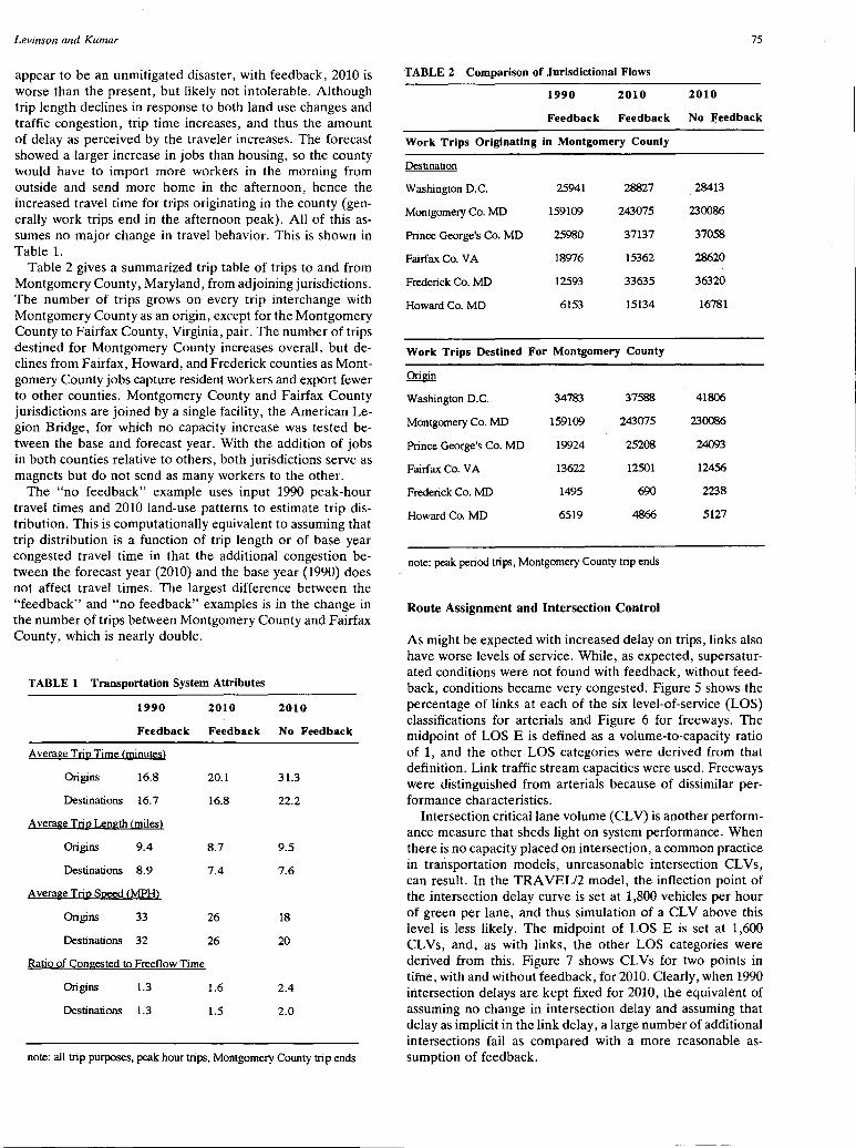
Levinson and Kumar

appear to be an unmitigated disaster, with feedback, 2010 is worse than the present, but likely not intolerable. Although trip length declines in response to both land use changes and traffic congestion, trip time increases, and thus the amount of delay as perceived by the traveler increases. The forecast showed a larger increase in jobs than housing, so the county would have to import rriore workers in the morning from outside and send more home in the afternoon, hence the increased travel time for trips originating in the county (gen­erally work trips end in the afternoon peak). All of this as­sumes no major change in travel behavior. This is shown in Table 1.

Table 2 gives a summarized trip table of trips to and from Montgomery County, Maryland, from adjoining jurisdictions. The number of trips grows on every trip interchange with Montgomery County as an origin, except for the Montgomery County to Fairfax County, Virginia, pair. The number of trips destined for Montgomery County increases overall, but de­clines from Fairfax, Howard, and Frederick counties as Mont­gomery County jobs capture resident workers and export fewer to other counties. Montgomery County and Fairfax County jurisdictions are joined by a single facility, the American Le­gion Bridge, for which no capacity increase was tested be­tween the base and forecast year. With the addition of jobs in both counties relative to others, both jurisdictions serve as magnets but do not send as many workers to the other.

The "no feedback" example uses input 1990 peak-hour travel times and 2010 land-use patterns to estimate trip dis­tribution. This is computationally equivalent to assuming that trip distribution is a function of trip length or of base year congested travel time in that the additional congestion be­tween the forecast year (2010) and the base year (1990) does not affect travel times. The largest difference between the "feedback" and "no feedback" examples is in the change in the number of trips between Montgomery County and Fairfax County, which is nearly double.

TABLE 1 Transportation System Attributes

1990 2010 2010

Feedback Feedback No Feedback

Average Tri12 Time (minutes}

Origins 16.8 20.1 31.3

Destinations 16.7 16.8 22.2

Average Tri12 Length (miles}

Origins 9.4 8.7 9.5

Destinations 8.9 7.4 7.6

Average Tri12 S~ed (MPI::D

Origins 33 26 18

Destinations 32 26 20

Ratio of ~ongested to Freeflow Time

Origins 1.3 1.6 2.4

Destinations 1.3 1.5 2.0

note: all trip purposes, peak hour trips, Montgomery County trip ends

75

TABLE 2 Comparison of Jurisdictional Flows

1990 2010 2010

Feedback Feedback No ~eedback

Work Trips Originating in Montgomery County

Destination

Washington D.C. 25941 28827 28413

Montgomery Co. MD 159109 243075 230086

Prince George's Co. MD 25980 37137 37058

Fairfax Co. VA 18976 15362 28620

Frederick Co. MD 12593 33635 36320

Howard Co. MD 6153 15134 16781

Work Trips Destined For Montgomery County

Origin

Washington D.C. 34783 37588 41806

Montgomery Co. MD 159109 243075 230086

Prince George's Co. MD 19924 25208 24093

Fairfax Co. VA 13622 12501 12456

Frederick Co. MD 1495 690 2238

Howard Co. MD 6519 4866 5127

note: peak period trips, Montgomery County trip ends

Route Assignment and Intersection Control

As might be expected with increased delay on trips, links also have worse levels of service. While, as expected, supersatur­ated conditions were not found with feedback, without feed­back, conditions became very congested. Figure 5 shows the percentage of links at each of the six level-of-service (LOS) classifications for arterials and Figure 6 for freeways. The midpoint of LOS E is defined as a volume-to-capacity ratio of 1, and the other LOS categories were derived from that definition. Link traffic stream capacities were used. Freeways were distinguished from arterials because of dissimilar per­formance characteristics.

Intersection critical lane volume (CLV) is another perform­ance measure that sheds light on system performance. When there is no capacity placed on intersection, a common practice in transportation models, unreasonable intersection CLVs, can result. In the TRAVEL/2 model, the inflection point of the intersection delay curve is set at 1,800 vehicles per hour of green per lane, and thus simulation of a CL V above this level is less likely. The midpoint of LOS E is set at 1,600 CLVs, and, as with links, the other LOS categories were derived from this. Figure 7 shows CLVs for two points in tifiie, with and without feedback, for 2010. Clearly, when 1990 intersection delays are kept fixed for 2010, the equivalent of assuming no change in intersection delay and assuming that delay as implicit in the link delay, a large number of additional intersections fail as compared with a more reasonable as­sumption of feedback.

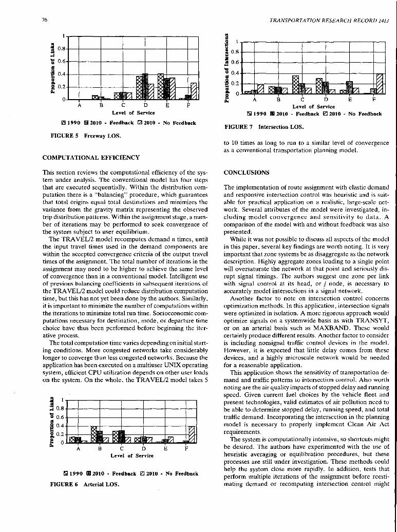
76

i o.s-----------~ ..3

~ 0.6-t---+---+----+----+-----+----+-----1 Ii:!

·e 0.4-t---t---+--+---0 1111'1 e o.2-+--+---+---l---1)(.)

"" A B C D

Level of Service E F

~ 1990 1112010 - Feedback 1:2! 2010 - No Feedback

FIGURE 5 Freeway LOS.

COMPUTATIONAL EFFICIENCY

This section reviews the computational efficiency of the sys­tem under analysis. The conventional model has four steps that are executed sequentially. Within the distribution com­putation there is a "balancing" procedure, which guarantees that total origins equal total destinations and minimizes the variance from the gravity matrix representing the observed trip distribution patterns. Within the assignment stage, a num­ber of iterations may be performed to seek convergence of the system subject to user equilibrium.

The TRAVEL/2 model recomputes demand n times, until the input travel times used in the demand components are within the accepted convergence criteria of the output travel times of the assignment. The total number of iterations in the assignment may need to be higher to achieve the same level of convergence than in a conventional model. Intelligent use of previous balancing coefficients in subsequent iterations of the TRA VEL/2 model could reduce distribution computation time, but this has not yet been done by the authors. Similarly, it is important to minimize the number of computations within the iterations to minimize total run time. Socioeconomic com­putations necessary for destination, mode, or departure time choice have thus been performed before beginning the iter­ative process.

The total computation time varies depending on initial start­ing conditions. More congested networks take considerably longer to converge than less congested networks. Because the application has been executed on a multiuser UNIX operating system, efficient CPU utilization depends on other user loads on the system. On the whole, the TRA VEL/2 model takes 5

~ o.~---+----+-----1----ii---_,1------1-~ .. 0 0.6 +---+---+----+-------+----+---i Ii:! ·e 0.4 +--+----.......-+---+-----+-----t----+---rl

& 0.2 +--+--tK; e o..l..IQoiliiljliilO ....... _

"" A B c D E F Level of Service

!Sil 1990 Ill 2010 - Feedback IZ'.l 2010 - No Feedback

FIGURE 6 Arterial LOS.

TRANSPORTATION RESEARCH RECORD 1413

a ·! u !! 0.8 ----------+-----+------1----t--'1

I o.6 +--+-----+----1-----+-----i----+--l .... .. 0 0.4 ...--r----;----ir----t-----t----t--r--i Ii:!

·e o. 2 +--t-;;=;;-__,1-----f..X..

& 0 e ~~ ..... ~ c:i.. A B c D E F

Level of Service !Sil 1990 11112010 - Feedback IZ'.l 2010 - No Feedback

FIGURE 7 Intersection LOS.

to 10 times as long to run to a similar level of convergence as a conventional transportation planning model.

CONCLUSIONS

The implementation of route assignment with elastic demand and responsive intersection control was heuristic and is suit­able for practical application on a realistic, large-scale net­work. Several attributes of the model were investigated, in­cluding model convergence and sensitivity to data. A comparison of the model with and without feedback was also presented.

While it was not possible to discuss all aspects of the model in this paper, several key findings are worth noting. It is very important that zone systems be as disaggregate as the network description. Highly aggregate zones loading to a single point will oversaturate the network at that point and seriously dis­rupt signal timings. The authors suggest one zone per link with signal control at its head, or j node, is necessary to accurately model intersections in a signal network.

Another factor to note on intersection control concerns optimization methods. In this application, intersection signals were optimized in isolation. A more rigorous approach would optimize signals on a systemwide basis as with TRANSYT, or on an arterial basis such as MAXBAND. These would certainly produce different results. Another factor to consider is including nonsignal traffic control devices in the model. However, it is expected that little delay comes from these devices, and a highly microscale network would be needed for a reasonable application.

This application shows the sensitivity of transportation de­mand and traffic patterns to intersection control. Also worth noting are the air quality impacts of stopped delay and running speed. Given current fuel choices by the vehicle fleet and present technologies, valid estimates of air pollution need to be able to determine stopped delay, running speed, and total traffic demand. Incorporating the intersection in the planning model is necessary to properly implement Clean Air Act requirements.

The system is computationally intensive, so shortcuts might be desired. The authors have experimented with the use of heuristic averaging or equilibration procedures, but these processes are still under investigation. These methods could help the system close more rapidly. In addition, tests that perform multiple iterations of the assignment before reesti­mating demand or recomputing intersection control might

Levinson and Kumar

converge the system more quickly with little degradation of results, but this awaits further research.

Application of this model produces forecasts that the model developers consider more reasonable than using a simplistic four-step approach. The authors are aware that technological or behavioral change makes all long-term forecasting suspect; however, even for short-term planning, it is necessary to have an idea of what the "best guess" future might be. With feed­back, congestion increases with faster growth in land use than network. In the application presented here, travel times in­crease, primarily in response to an increased job/housing ratio moving the system from a balance where the number of jobs and resident workers in Montgomery County is about equal to a skew toward jobs. Considering the historical stability of travel times for work trips, this may suggest that land-use forecasts are predicting more jobs than transportation acces­sibility would provide. Incorporation of a land-use allocation model may alleviate this discrepancy. Clearly location choice is in part a function of transportation accessibility. When land­use forecasts are performed independently of transportation analysis, a "no feedback" situation exists, which may over­represent one element of the system at the expense of others.

A second obvious extension of this model is to the network design problem (NDP). The NDP attempts to determine the optimal sequence of increasing transportation supply by com­paring different alternatives on a common basis, such as total travel time in the system. The NDP has traditionally assumed static demand. However, with the ability to reasonably fore­cast changes in demand with respect to congestion, developing rankings of benefits in reduced system travel time given by additional facilities is a promising area of research.

ACKNOWLEDGMENTS

The authors would like to acknowledge Bob Winick and Mi­chael Replogle, both formerly of the Montgomery County Planning Department. The authors would also like to thank in particular Everett Carter and Paul Schonfeld of the Uni­versity of Maryland and Gang Len Chang for their comments on an earlier draft of this work, which was part of the master's thesis of David Levinson. The Transportation Modeling Tech­nical Advisory Committee of the MCPD has served as a sounding board and forum for many of the ideas herein. The patience and assistance of numerous other staff of the Mont­gomery County Planning Department have made this effort possible.

REFERENCES

1. Meyer, M. D., and E. J. Miller. Urban Transportation Planning: A Decision-Oriented Approach, McGraw Hill, New York, 1984.

2. Levinson, D. M. An Integrated Transportation Planning Model. M.S. thesis. University of Maryland, College Park, 1991.

3. Horowitz, A. J. Implementing Travel Forecasting with Traffic Operational Strategies. In Transportation Research Record 1365, TRB, National Research Council, Washington, D.C., 1992.

77

4. Evans, S. P. Derivation and Analysis of Some Models for Com­bining Trip Distribution and Assignment. Transportation Re­search, Vol. 10, 1976, pp. 37-57.

5. Florian, M., S. Nguyen, and J. Ferland. On the Combined Distribution-Assignment of Traffic. Transportation Science, Vol. 9, 1975, pp. 43-53.

6. Boyce, D. E., L. LeBlanc, and K. Chon. Network Equilibrium Models of Urban Location and Travel Choices: A Retrospective Survey. Journal of Regional Science, Vol. 28, No. 2, 1988.

7. Smith, M. J. Traffic Control and Route Choice; A Simple Ex­ample. Transportation Research B, Vol. 13B, 1979, pp. 289-294.

8. Charlesworth, J. A. The Calculation of Mutually Consistent Sig­nal Settings and Traffic Assignment for a Signal-Controlled Road Network. Transport Operations Research Group, University of Newcastle-upon-Tyne, United Kingdom, 1977.

9. Tan, H., S. Gershwin, and M. Athans. Hybrid Optimization in Urban Traffic Networks. Report DOT-TSC-RSPA-79-7. FHWA, U.S. Department of Transportation, 1979.

10. Smith, M. J. The Existance, Uniqueness and Stability of Traffic Equilibria. Transportation Research B, Vol. 13B, 1979, pp. 295-304.

11. Smith, M. J. Properties of a Traffic Control Policy Which Ensure the Existence of Traffic Equilibrium Consistent with the Policy. Transportation Research B, Vol. 15B, No. 6, 1981, pp. 453-462.

12. Smith, M. J. The Existence of an Equilibrium Solution to the Traffic Assignment Problem When There are Junction Inter­actions. Transportation Research B, Vol. 15B, No. 6, 1981, pp. 443-451.

13. Smith, M. J. Junction Interactions and Monotonicity in Traffic Assignment. Transportation Research B, Vol. 16B, No. 1, 1982, pp. 1-3.

14. Smith, M. J. The Existence and Calculation of Traffic Equilibria. Transportation Research B, Vol. 17B, No. 4, 1983, pp. 291-303.

15. Smith, M. J. Traffic Signals in Assignment. Transportation Re­search B, Vol. 19B, No. 2, 1985, pp. 155-160.

16. Smith, M. J., and M. Ghali. The Dynamics of Traffic Assignment and Traffic Control: A Theoretical Study. Transportation Re­search B, Vol. 24B, No. 6, 1990, pp. 409-422.

17. Van Vuren, T., M. J. Smith, and D. Van Vliet. The Interaction Between Signal Setting Optimization and Reassignment: Back­ground and Preliminary Results. In Transportation Research Rec­ord 1142, TRB, National Research Council, Washington, D.C., 1988.

18. Replogle, M. Computer Transportation Models for Land Use Regulation and Master Planning in Montgomery County, Md. In Transportation Research Record 1262, TRB, National Research Council, Washington, D.C., 1990, pp. 91-100.

19. Round IV Cooperative Forecast. Metropolitan Washington Coun­cil of Governments, Washington, D.C., 1989.

20. Round IV Cooperative Forecast. Metropolitan Baltimore Council of Governments, Baltimore, Md., 1991.

21. Kumar, A., and D. Levinson. TRA VEL/2 Model Technical Doc­umentation. Montgomery County Planning Department, Silver Spring, Md., 1991.

22. Levinson, D. TRA VEL/2 User's Guide. Montgomery County Planning Department, Silver Spring, Md., 1991.

23. Levinson, D. Empirical Estimation of Speed Flow and Density on Signalized Arterials. Working paper, 1992.

24. Hurdle, V. Signalized Intersection Delay Models: A Primer for the Uninitiated. In Transportation Research Record 971, TRB, National Research Council, Washington, D.C., 1984.

25. McShane, W., and R. Roess. Traffic Engineering. Prentice-Hall, Englewood Cliffs, N.J., 1990.

26. Special Report 209: Highway Capacity Manual. TRB, National Research Council, Washington, D.C., 1985.

Publication of this paper sponsored by Committee on Passenger Travel Demand Forecasting.

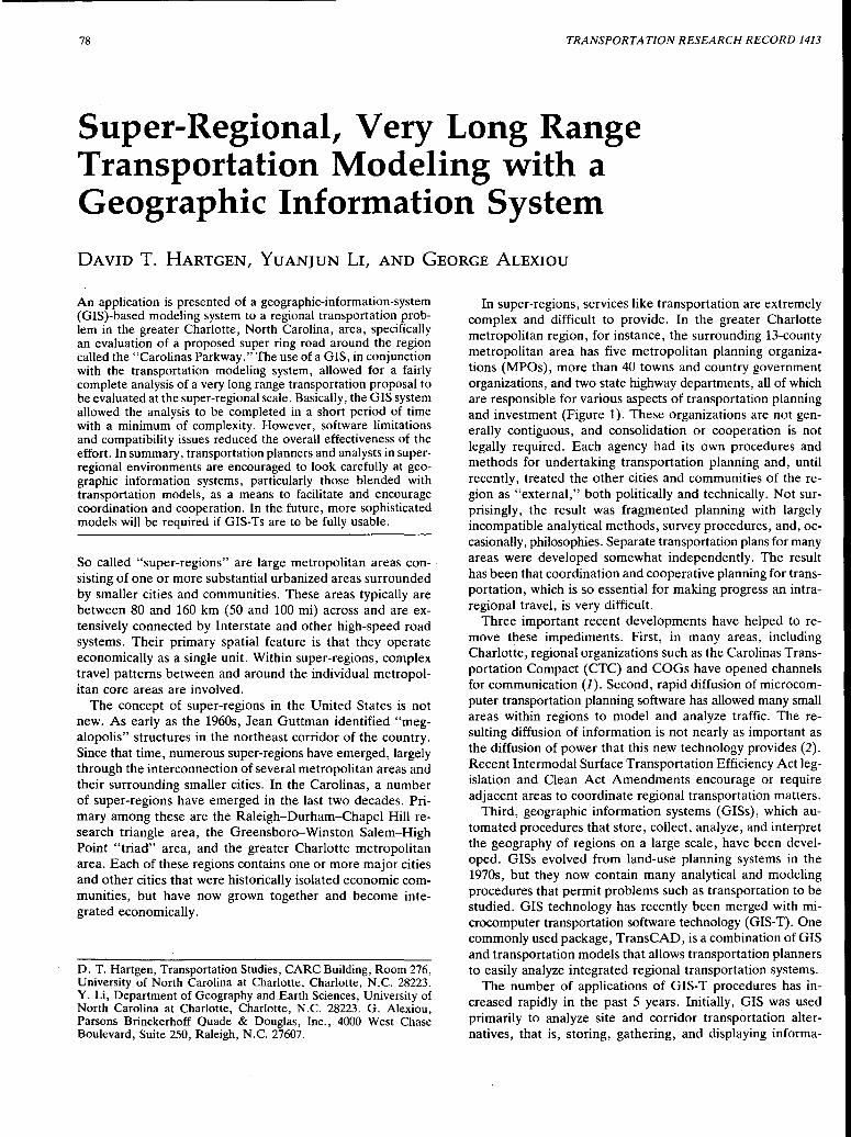
78 TRANSPORTATION RESEARCH RECORD 1413

Super-Regional, Very Long Range Transportation Modeling with a Geographic Information System

DAVID T. HARTGEN, YuANJUN LI, AND GEORGE ALEXIOU

An application is presented of a geographic-information-system (GIS)-based modeling system to a regional transportation prob­lem in the greater Charlotte, North Carolina, area, specifically an evaluation of a proposed super ring road around the region called the "Carolinas Parkway." The use of a GIS, in conjunction with the transportation modeling system, allowed for a fairly complete analysis of a very long range transportation proposal to be evaluated at the super-regional scale. Basically, the GIS system allowed the analysis to be completed in a short period of time with a minimum of complexity. However, software limitations and compatibility issues reduced the overall effectiveness of the effort. In summary, transportation planners and analysts in super­regional environments are encouraged to look carefully at geo­graphic information systems, particularly those blended with transportation models, as a means to facilitate and encourage coordination and cooperation. In the future, more sophisticated models will be required if GIS-Ts are to be fully usable.

So called "super-regions" are large metropolitan areas con- · sisting of one or more substantial urbanized areas surrounded by smaller cities and communities. These areas typically are between 80 and 160 km (50 and 100 mi) across and are ex­tensively connected by Interstate and other high-speed road systems. Their primary spatial feature is that they operate economically as a single unit. Within super-regions, complex travel patterns between and around the individual metropol­itan core areas are involved.

The concept of super-regions in the United States is not new. As early as the 1960s, Jean Guttman identified "meg­alopolis" structures in the northeast corridor of the country. Since that time, numerous super-regions have emerged, largely through the interconnection of several metropolitan areas and their surrounding smaller cities. In the Carolinas, a number of super-regions have emerged in the last two decades. Pri­mary among these are the Raleigh-Durham-Chapel Hill re­search triangle area, the Greensboro-Winston Salem-High Point "triad" area, and the greater Charlotte metropolitan area. Each of these regions contains one or more major cities and other cities that were historically isolated economic com­munities, but have now grown together and become inte­grated economically.

D. !· H_artgen, Transportation Studies, CARC Building, Room 276, Umvers1ty of North Carolina at Charlotte, Charlotte, N.C. 28223. Y. Li, Department of Geography and Earth Sciences, University of North Carolina at Charlotte, Charlotte, N.C. 28223. G. Alexiou, Parsons Brinckerhoff Quade & Douglas, Inc., 4000 West Chase Boulevard, Suite 250, Raleigh, N.C. 27607.

In super-regions, services like transportation are extremely complex and difficult to provide. In the greater Charlotte metropolitan region, for instance, the surrounding 13-county metropolitan area has five metropolitan planning organiza­tions (MPOs), more than 40 towns and country government organizations, and two state highway departments, all of which are responsible for various aspects of transportation planning and investment (Figure 1). These organizations are not gen­erally contiguous, and consolidation or cooperation is not legally required. Each agency had its own procedures and methods for undertaking transportation planning and, until recently, treated the other cities and communities of the re­gion as "external," both politically and technically. Not sur­prisingly, the result was fragmented planning with largely incompatible analytical methods, survey procedures, and, oc­casionally, philosophies. Separate transportation plans for many areas were developed somewhat independently. The result has been that coordination and cooperative planning for trans­portation, which is so essential for making progress an intra­regional travel, is very difficult.

Three important recent developments have helped to re­move these impediments. First, in many areas, including Charlotte, regional organizations such as the Carolinas Trans­portation Compact (CTC) and COGs have opened channels for communication (1). Second, rapid diffusion of microcom­puter transportation planning software has allowed many small areas within regions to model and analyze traffic. The re­sulting diffusion of information is not nearly as important as the diffusion of power that this new technology provides (2). Recent Intermodal Surface Transportation Efficiency Act leg­islation and Clean Act Amendments encourage or require adjacent areas to coordinate regional transportation matters.

Third, geographic information systems (GISs), which au­tomated procedures that store, collect, analyze, and interpret the geography of regions on a large scale, have been devel­oped. GISs evolved from land-use planning systems in the 1970s, but they now contain many analytical and modeling procedures that permit problems such as transportation to be studied. GIS technology has recently been merged with mi­crocomputer transportation software technology (GIS-T). One commonly used package, TransCAD, is a combination of GIS and transportation models that allows transportation planners to easily analyze integrated regional transportation systems.

The number of applications of GIS-T procedures has in­creased rapidly in the past 5 years. Initially, GIS was used primarily to analyze site and corridor transportation alter­natives, that is, storing, gathering, and displaying informa-

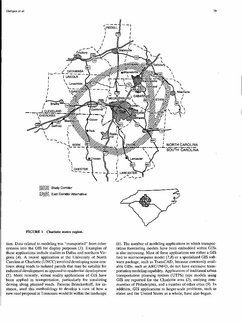
Hartgen et al. 79

\1;E0Eli.

- ---,</

~ Study Corridor ,;i;t ·~~ ~~~<'I East Corridor Alternative

FIGURE 1 Charlotte metro region.

I

I I

I

tion. Data related to modeling was "transported" from other systems into the GIS for display purposes (3). Examples of these applications include studies in Dallas and northern Vir­ginia (4). A recent application at the University of North Carolina at Charlotte (UNCC) involved developing noise con­tours along roads to isolated parcels that may be suitable for industrial development as opposed to residential development (5). More recently, virtual reality applications of GIS have been applied in transportation, particularly for simulating driving along planned roads. Parsons Brinckerhoff, for in­stance, used this methodology to develop a view of how a new road proposal in Tennessee would fit within the landscape

I I I

- _j LANCASTER I ,,,, 1_,,,,

I I

.l.~~~-~~~l~A SOUTH CAROLINA

(6). The number of modeling applications in which transpor­tation forecasting models have been embedded within GISs is also increasing. Most of these applications use either a GIS tied to microcomputer model (7,8) or a specialized GIS soft­ware package, such as TransCAD, because commonly avail­able GISs, such as ARC/INFO, do not have extensive trans­portation modeling capability. Applicatipns of traditional urban transportation planning system (UTPS) type models using GIS are reported for the Charlotte area (2), outlying com­munities of Philadelphia, and a number of other cities (9). In addition, GIS applications to larger-scale problems, such as states and the United States as a whole, have also begun.

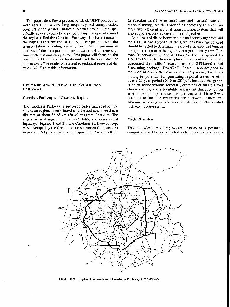
80

This paper describes a process by which GIS-T procedures were applied to a very long range regional transportation proposal in the greater Charlotte, North Carolina, area, spe­cifically an evaluation of the proposed super ring road around the region called the Carolinas Parkway. The basic theme of the paper is that the use of a GIS, in conjunction with the transportation modeling system, permitted a preliminary analysis of the transportation proposal in a short period of time with minimal complexity. This paper will focus on the use of this GIS-T and its limitations, not the evaluation of alternatives. The reader is referred to technical reports of the study (10-12) for this information.

GIS MODELING APPLICATION: CAROLINAS PARKWAY

Carolinas Parkway and Charlotte Region

The Carolinas Parkway, a proposed outer ring road for the Charlotte region, is envisioned as a limited access road at a distance of about 32-65 km (20-40 mi) from Charlotte. The ring road is designed to link I-77, I-85, and other radial highways (Figures 1 and 2). The Carolinas Parkway concept was developed by the Carolinas Transportation Compact (13) as part of a 50-year long-range transportation "vision" effort.

TRANSPORTATION RESEARCH RECORD 1413

Its function would be to coordinate land use and transpor­tation planning, which is viewed as necessary to create an attractive, efficient regional transportation system that will also support economic development objectives.

As a result of dialog between state and county agencies and the CTC, it was agreed that the Carolinas Parkway concept should be tested to determine the travel efficiency and benefit it might contribute to the region's transportation system. Par­sons Brinckerhoff Quade & Douglas, Inc., supported by UNCC's Center for Interdisciplinary Transportation Studies, conducted the traffic forecasting using a GIS-based travel forecasting package, TransCAD. Phase 1 was designed to focus on assessing the feasibility of the parkway by deter­mining its potential for generating regional travel benefits over a 20-year period (2010 to 2030). It included the gener­ation of socioeconomic forecasts, estimates of future travel characteristics, and a feasibility assessment that focused on environmental impact issues and parkway cost. Phase 2 was designed to focus on optimizing the parkway location, ex­amining partial ring road concepts, and identifying other needed highway improvements.

Model Overview

The TransCAD modeling system consists of a personal­computer-based GIS augmented with numerous procedures

FIGURE 2 Regional network and Carolinas Parkway alternatives.

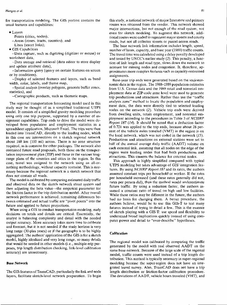
Hartgen et al.

for transportation modeling. The GIS portion contains the usual features and capabilities:

•Layers -Points (cities, nodes), -Areas (zones, tracts, counties), and - Lines (street links);

• GIS Capabilities -Data capture, such as digitizing (digitizer or mouse) or

worksheet data, - Data storage and retrieval (data editor to store display

and update attribute data), - Information query (query on certain features on screen

or by conditions), - Display of selected features and layers, such as band

width, color, labels, and theme map, -Spatial analysis (overlay polygons, generate buffer zones,

statistics), and -Cartographic products, such as thematic maps.

The regional transportation forecasting model used in this study may be thought of as a simplified traditional UTPS m?del. It consists of a simplified gravity modeiing procedure usmg only one trip purpose, supported by a number of as­signment capabilities. Trip ends to drive the model were de­veloped from population and employment statistics in a spreadsheet application, Microsoft Excel. The trips were then loaded into TransCAD, directly to the loading nodes, which in this case are intersections on a sketch regional network about 160 km (100 mi) across. There is no zone structure required, as is common for other packages. The network also co~tai~ed future road proposals, both those on the transpor­tation improvement plan (TIP) and those in the various long­range plans of the counties and cities in the region. In this case, travel was assigned to the network using an all-or­nothing methodology, without capacity restraint. This is nec­essary because the regional network is a sketch network that does not contain all roads.

The model is calibrated by comparing estimated daily traffic and observed data on the sketch network street system and then adjusting the beta value-the empirical parameter for the friction factor in the trip distribution model. After overall network performance is achieved, remaining differences be­tween estimated and actual traffic are "pivot points" into the future and applied to future projections. ~en using a GIS to conduct transportation modeling, early

declSlon~ on totals and details are critical. Essentially, the analyst is balancing complexity and detail with the needed output accuracy. More accuracy takes more time to calibrate and forecast, but it is not needed if the study horizon is very long rarrge (30-plus years) or if the geography is to be highly aggregated. The authors' application of the GIS is for a sketch model, highly idealized and very long range, so many details that wou~d be needed in other models (i.e., multiple-trip pur­poses, tnp length distribution checking, link-level calibration accuracy) are unnecessary.

Base Network

The GIS features ofTransCAD, particularly the link and node layers, facilitate sketch-level network preparation. To begin

81

this study, a national network of major Interstate and primary routes was obtained from the vendor. This network showed major intersections, but not enough of the road system, not even for sketch modeling. To augment this network addi­tional routes were coded to represent major streets and ~ounty roads, but not all collector streets or parcel-access roads.

The base network link information includes length, speed, number of lanes, capacity, and base year (1989) traffic counts. The travel time was calculated using a delay penalty developed and tested by UNCC's earlier study (2). This penalty, a func­tion of link length and road type, slows down the network to acco~nt for missing nodes and congestion. It, therefore, ap­proximates more complex features such as capacity-restrained assignments.

Base-year trip ends were generated based on the socioeco­nomic data in the region. The 1988-1989 population estimates from U.S. Census data and the 1989 retail and nonretail em­pl.oyment d~ta at ZIP-code zone level were used to generate tnp productions and attractions. Rather than use the "traffic analysis zone" method to locate the population and employ­ment data, the data were directly tied to selected loading nodes on the network (2). Vehicle trip ends were derived from dwelling units, retain employment, and nonretail em­ployment according to the procedures in Table 3 of NCHRP Report 187 (14). It should be noted that a deduction factor of 0. 721 was applied to the trip ends, because about 28 per­cent of the vehicle miles traveled (VMT) in the region is on the loca! network, whic~ was not coded in the network (15). Productions and attractions on external stations were set to half of the annual average daily traffic (AADT) volume on eac~ external link~ assuming that all nodes on the edge of the region were loadmg nodes that had both productions and attractions. This ensures the balance for external nodes.

This approach is highly simplified compared with typical UTPS modeling but takes advantage of GIS' integration fea­tures. By using NCHRP Report 187 and its rates, the authors assumed constant trips per household or worker. If the rates per household increased (and these rates generally did not, rates per person did), then the method would underestimate future traffic. By using a reduction factor, the authors as­sumed a constant ratio of travel on high and low facilities. While these ratios may be different in the future, the authors had no basis for changing them. A better procedure the authors believe, would be to use this GIS-T to test ~any futures instead of trying to detail a few. This is the essence of sketch playing with a GIS-T: use speed and flexibility to understand broad implications quickly instead of using com­puter power and detail to "over-describe" hypotheses.

Calibration

The regional model was calibrated by comparing the traffic generated by the model with real observed AADT on the same base network. Because of the large scale of the regional model, traffic counts were used instead of a trip length dis­tributi?n. This method is typically necessary in super-regional modelmg because the super-region does not have an inte­grated travel survey. Also, TransCAD does not have a trip length distribution or friction-factor calibration procedure. The deviations of AADT, vehicle hours traveled (VHT), and

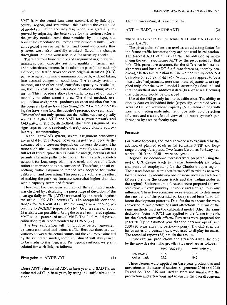
82

VMT from the actual data were summarized by link type, county, region, and screenlines; this assisted the evaluation of model simulation accuracy. The model was gradually im­proved by adjusting the beta value for the friction factor in the gravity model, travel time penalties by link type, and travel time impedance values for a few individual links. Over­all regional average trip length and county-to-county flow patterns were also carefully checked. Screenline changes throughout the area were also used for accuracy checks.

There are four basic methods of assignment in general use: minimum path, capacity restraint, equilibrium assignment, and stochastic assignment. In the minimum path (all-or-nothing) method, the traffic flows for each origin-destination (0-D) pair is assigned the single minimum cost path, without taking into account congestion conditions. The capacity restraint method, on the other hand, considers capacity by recalculat­ing the link costs at each iteration of all-or-nothing assign­ments. This procedure allows the traffic to spread out incre­mentally to other street routes. The third method, user equilibrium assignment, produces an exact solution that has the property that no travel can change routes without increas­ing the travel time (i.e., the traveler's presence slows all traffic). This method not only spreads out the traffic, but also typically results in higher VHT and VMT for a given network and 0-D pattern. The fourth method, stochastic assignment, as­signs trips to paths randomly, thereby more closely approx­imately user uncertainty.

In the TransCAD system, several assignment procedures are available. The choice, however, is not trivial because the accuracy of the forecast depends on network diversity. The more sophisticated procedures are commonly used when (a) full set of trip purpose data is available and (b) network detail permits alternate paths to be chosen. In this study, a sketch network for long-range planning is used, and overall effects rather than minor ones are considered. Therefore, the all-or­nothing traffic assignment method was adopted for traffic calibration and forecasting. This procedure will have the effect of making the parkway forecasts somewhat higher than that with a capacity-restrained forecast.

However, the base-year accuracy of the calibrated model was checked by calculating the percentage of deviation of the average daily traffic (ADT) estimated by the model against the actual 1989 ADT counts (2). The acceptable deviation ranges for different ADT volume ranges were defined ac­cording to NCHRP Report 255 (16). Over a series of about 25 trials, it was possible to bring the overall estimated regional VMT to ± 1 percent of actual VMT. The final model passed calibration tests recommended by FHWA (17).

The best calibration will not produce perfect agreement between estimated and actual traffic. Because there are de­viations between the actual counts and the volumes estimated by the calibrated model, some adjustment will always need to be made to the forecasts. Pivot-point methods were cal­culated for each link, as follows:

Pivot point = ADT/EADT (1)

where ADT is the actual ADT in base year and EADT is the estimated ADT in base year, by using the traffic simulation model.

TRANSPORTATION RESEARCH RECORD 1413

Then in forecasting, it is assumed that

ADT1 = EADT1 * (ADT/EADT) (2)

where ADT1 is the future actual ADT and EADT1 is the future EADT.

The pivot-point values are used as an adjusting factor for the future traffic forecasts; they are not used in calibration. The forecast ADT of a link can then be obtained by multi­plying the estimated future ADT by the pivot point for that link. This procedure accounts for the difference in base as­signments and base ADT for future forecasts, thereby pro­ducing a better future estimate. The method is fully described by Pederson and Samdahl (16). While it may appear to be a "hard-wire" adjustment, note that these adjustments are ap­plied only after the overall model is accurately calculated and that the method uses additional data (base-year ADT counts) that otherwise would be discarded.

Use of the GIS greatly facilitates calibration. The ability to display data on individual links (especially, estimated versus actual ADT, on volume-to-capacity (V/C) ratios) along with zonal and loading node information, permits rapid detection of errors and a clear, broad view of the entire system's per­formance by area or facility type.

Forecasts

For traffic forecasts, the road network was expanded by the addition of planned roads in the formalized TIP and long­range thoroughfare plans. Two future Carolinas Parkway net­works-2010 and 2030-were analyzed.

Regional socioeconomic forecasts were prepared using the unit of U.S. Census tracts to forecast households and retail and nonretail employment for the Charlotte super-region. These tract forecasts were then "attached" to existing network loading nodes, by identifying one or more nodes in each tract (Figure 3 shows the census tracts and the loading nodes in the region). Socioeconomic forecasts were prepared for two scenarios: a "low" parkway influence and a "high" parkway influence. These two scenarios were evaluated to determine the sensitivity of the potential parkway travel benefits to dif­ferent development patterns. Data for the two scenarios were converted to trip productions and attractions in terms of the same methods used in the calibrated model. Also, the same deduction factor of 0. 721 was applied to the future trip ends for the sketch network effects. Forecasts were prepared for years 2010 (the assumed year that the parkway opens) and 2030 (20 years after the parkway opens). The GIS structure for counties and census tracts was used to display forecasts. The technical report (12) details the results.

Future external productions and attractions were factored by the growth rates. The growth rates used are as follows:

1989-2010 (%) 1989-2030 (%)

Interstates 31.5 61.5 Other roads 25.2 49.2

These factors were applied on base-year productions and attractions ,at the external stations to generate 2010 and 2030 Ps and As. The GIS was used to store and manipulate the production and attractions and to ensure the overall regional

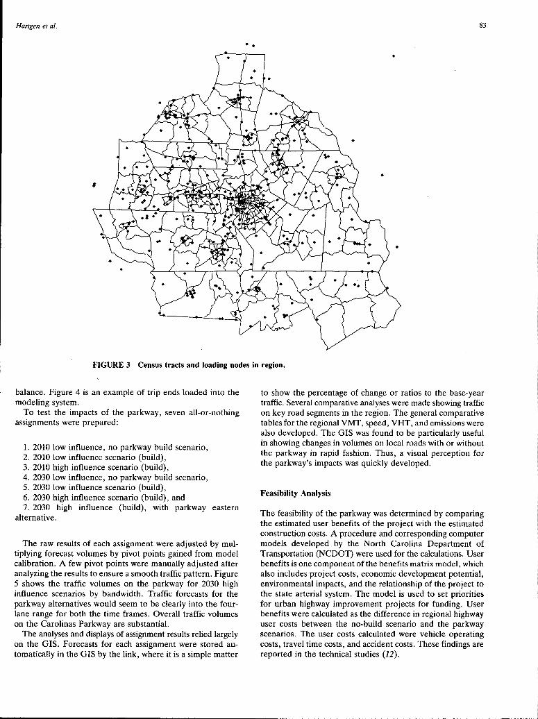
Hartgen et al. 83

• •

FIGURE 3 Census tracts and loading nodes in region.

balance. Figure 4 is an example of trip ends loaded into the modeling system.

To test the impacts of the parkway, seven all-or-nothing assignments were prepared:

1. 2010 low influence, no parkway build scenario, 2. 2010 low influence scenario (build), 3. 2010 high influence scenario (build), 4. 2030 low influence, no parkway build scenario, 5. 2030 low influence scenario (build), 6. 2030 high influence scenario (build), and 7. 2030 high influence (build), with parkway eastern

alternative.

The raw results of each assignment were adjusted by mul­tiplying forecast volumes by pivot points gained from model calibration. A few pivot points were manually adjusted after analyzing the results to ensure a smooth traffic pattern. Figure 5 shows the traffic volumes on the parkway for 2030 high influence scenarios by bandwidth. Traffic forecasts for the parkway alternatives would seem to be clearly into the four­lane range for both the time frames. Overall traffic volumes on the Carolinas Parkway are substantial.

The analyses and displays of assignment results relied largely on the GIS. Forecasts for each assignment were stored au­tomatically in the GIS by the link, where it is a simple matter

to show the percentage of change or ratios to the base-year traffic. Several comparative analyses were made showing traffic on key road segments in the region. The general comparative tables for the regional VMT, speed, VHT, and emissions were also developed. The GIS was found to be particularly useful in showing changes in volumes on local roads with or without the parkway in rapid fashion. Thus, a visual perception for the parkway's impacts was quickly developed.

Feasibility Analysis

The feasibility of the parkway was determined by comparing the estimated user benefits of the project with the estimated construction costs. A procedure and corresponding computer models developed by the North Carolina Department of Transportation (NCDOT) were used for the calculations. User benefits is one component of the benefits matrix model, which also includes project costs, economic development potential, environmental impacts, and the relationship of the project to the state arterial system. The model is used to set priorities for urban highway improvement projects for funding. User benefits were calculated as the difference in regional highway user costs between the no-build scenario and the parkway scenarios. The user costs calculated were vehicle operating costs, travel time costs, and accident costs. These findings are reported in the technical studies (12).

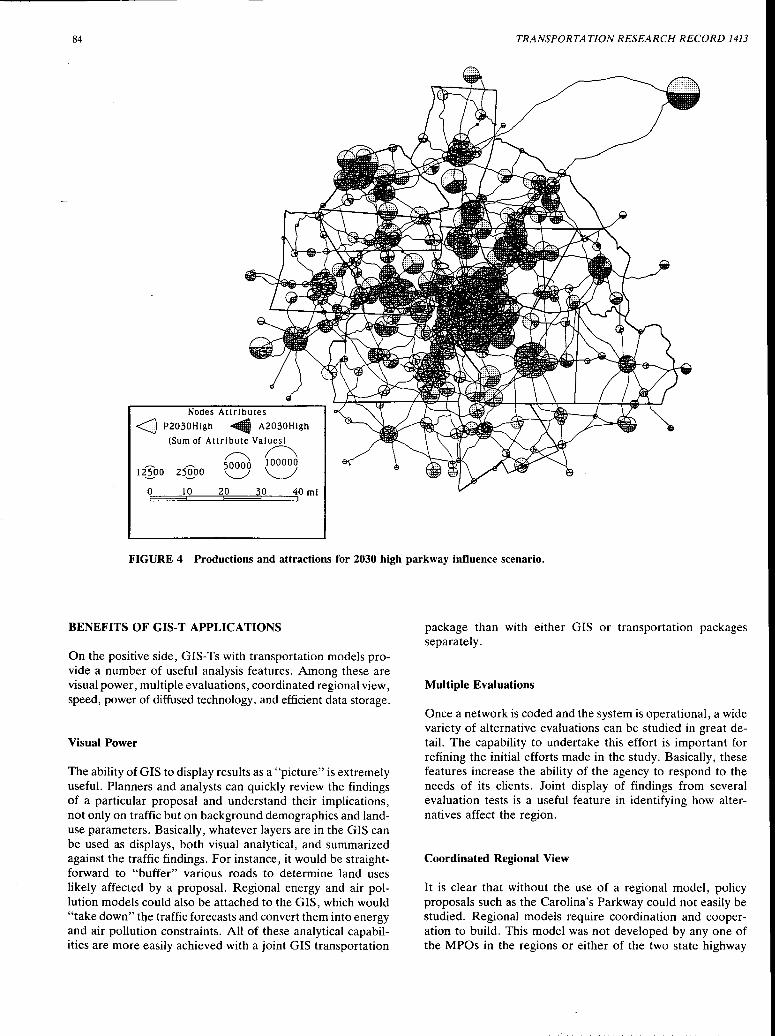
84

Nodes Attributes

<1@ P2030High ~ A2030High (Sum of Attribute Values)

~(\ 50000 100000

12100 2s]:oo '--...-/ \___/

OE· =:==:=1~0'.::::===2E0=:=~3~0=:==::540mi

TRANSPORTATION RESEARCH RECORD 1413

FIGURE 4 Productions and attractions for 2030 high parkway influence scenario.

BENEFITS OF GIS-T APPLICATIONS

On the positive side, GIS-Ts with transportation models pro­vide a number of useful analysis features. Among these are visual power, multiple evaluations, coordinated regional view, speed, power of diffused technology, and efficient data storage.

Visual Power

The ability of GIS to display results as a "picture" is extremely useful. Planners and analysts can quickly review the findings of a particular proposal and understand their implications, not only on traffic but on background demographics and land­use parameters. Basically, whatever layers are in the GIS can be used as displays, both visual analytical, and summarized against the traffic findings. For instance, it would be straight­forward to "buffer" various roads to determine land uses likely affected by a proposal. Regional energy and air pol­lution models could also be attached to the GIS, which would "take down" the traffic forecasts and convert them into energy and air pollution constraints. All of these analytical capabil­ities are more easily achieved with a joint GIS transportation

package than with either GIS or transportation packages separately.

Multiple Evaluations

Once a network is coded and the system is operational, a wide variety of alternative evaluations can be studied in great de­tail. The capability to undertake this effort is important for refining the initial efforts made in the study. Basically, these features increase the ability of the agency to respond to the needs of its clients. Joint display of findings from several evaluation tests is a useful feature in identifying how alter­natives affect the region.

Coordinated Regional View

It is clear that without the use of a regional model, policy proposals such as the Carolina's Parkway could not easily be studied. Regional models require coordination and cooper­ation to build. This model was not developed by any one of the MPOs in the regions or either of the two state highway

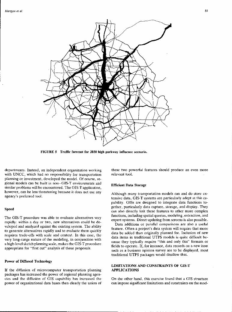
Hartgen et al. 85

FIGURE 5 Traffic forecast for 2030 high parkway influence scenario.

departments. Instead, an independent organization working with UNCC, which had no responsibility for transportation planning or investment, developed the model. Of course, re­gional models can be built in non-GIS-T environments and similar problems will be encountered. The GIS-T application, however, can be less threatening because it does not use any agency's preferred tool.

Speed

The GIS-T procedure was able to evaluate alternatives very rapidly: within a day or two, new alternatives could be de­veloped and analyzed against the existing system. The ability to generate alternatives rapidly and to evaluate them quickly requires trade-offs with scale and context. In this case, the very long-range nature of the modeling, in conjunction with a high-level sketch planning scale, makes the GIS-T procedure appropriate for "first cut" analysis of these proposals.

Power of Diffused Technology

If the diffusion of microcomputer transportation planning packages has increased the power of regional planning agen­cies and the diffusion of GIS capability has increased the power of organizational data bases then clearly the union of

these two powerful features should produce an even more relevant tool.

Efficient Data Storage

Although many transportation models can and do store ex­tensive data, GIS-T systems are particularly adept at this ca­pability. GISs are designed to integrate data functions to­gether, particularly data capture, storage, and display. They can also directly link these features to other more complex functions, including spatial queries, modeling, extraction, and expert systems. Direct updating from screens is also possible.

Data additions or parallel comparisons are also a useful feature. Often a project's data system will require that more data be added than originally planned for. Inclusion of new data items in traditional UTPS models is quite difficult be­cause they typically require "this and only this" formats or fields to operate. If, for instance, data records on a new item such as a business opinion survey are to be displayed, most traditional UTPS packages would disallow that.

LIMITATIONS AND CONSTRAINTS OF GIS-T APPLICATIONS

On the other hand, this exercise found that a GIS structure can impose significant limitations and constraints on the mod-

86

eling process. Among these are mismatches between GIS and transportation models, overly simple model extensions, lack of accuracy, and incompatability of results.

Mismatches Between GIS and Transportation Models

Blends of models sometimes produce a "camel," which is less functional than either of the original models. In some ways this is the case for GIS-T. Present GIS-Ts are not urban transportation planning models and do not have all the fea­tures that transportation planners expect. In particular, they are missing the following common features:

• Friction factors, • Multiple trip purposes, •Trip frequency distribution calibration, • Multipurpose gravity model, • Mode choice functions, •Trip generation function, •Automobile ownership forecasting, and •Speed feedbacks.

On the other hand, UTPS models typically do not have all the features of GISs. TransCAD, perhaps the most sophis­ticated GIS-T, lacks some of the geographical display and visual power of, say, ARC/INFO.

Overly Simple

Present GIS-Ts have essentially simple UTPS model exten­sions, which are generally too weak for many common mod­eling problems. For instance, TransCAD's trip-purpose lim­itations (one purpose only) effectively limits it to specialized, sketch-planning or one-purpose problems.

Lack of Accuracy

It proved difficult, even with extensive screenline and travel penalty adjustment, to calibrate the base model on a corridor or link-type basis. This is because, the authors suspect, that the one-trip-purpose requirement produces an average trip distribution that does not well replicate the multiple circum­stances of large complex regions. For sketch planning pur­poses, the calibration was sufficient, but it would be insuffi­cient for more sophisticated urban modeling. In forecasting, residual errors that would not be resolved in calibration were adjusted for through the pivot point procedure. This method, although acceptable also for sketch planning, is clearly less than ideal.

Incompatibility of Results

A continuing problem that GIS-T users will face, if they pro­pose to use GIS-T for modeling traffic, is a reluctance on the part of others to accept the results as valid. A recent survey of UTPS software technology (18) showed that the market of MPO users is divided as follows:

TRANSPORTATION RESEARCH RECORD 1413

Package

TRANPLAN MINUTP QRS, I and II TMODEL, I and II MICROTRIPS FSUMTS (Fla) Trans CAD EMME II Others

Percentage of Market

30 25 19 8 5 5 1 1 6

Of these, only TransCAD is generally recognized as a GIS-T, although other systems have some GIS-like fea,ures, particularly data display. It would therefore be understand­able that an agency familiar with the UTPS package would be reluctant to switch to a GIS-T or accept GIS-T results.

In this study, the final report (12) calls for remodeling the parkway sections in Phase 2 using a more traditional UTPS microcomputer model package. Given the model limitations, this is understandable. For closer-in analysis (fewer than 20 years) more confidence in the model and its forecasts is needed.

RECOMMEND A TIO NS

What should be done to facilitate GIS-T use and bring models together? The authors suggest the following:

•Vendors can develop smooth interfaces between GIS and transportation model packages. It should not be necessary to manually manipulate or repackage data to "see" results. A recent survey of systems (19) showed that of ten systems, four had GIS interfaces and three had GIS interfaces under development.

• More sophisticated GIS-T can be developed containing full-function UTPS models and GIS features together.

• Federal agencies and trade organizations can set stan­dards and guidelines for model use and operations, thereby encouraging the development of integrated tools.

• Applications developers can focus on targeted applica­tions that provide opportunities for blended methods. Several examples that could be explored are combination GIS-Air­Quality-UTPS models, models of intermodal transfer and operations, hazardous waste routing, route-corridor impact locations models, site-level impact models, and interstate­intercity model planning.

In summary, the opportunities for GIS-T packages in super­region contexts are extensive and essentially unexplored. Transportation planners and analysts in super-regional envi­ronments are encouraged to look carefully at geographical information systems, particularly those blended with trans­portation models, as a means to facilitate and encourage the coordination and cooperation that they have for so long asserted.

REFERENCES

1. Hartgen, D. T., and W. J. McCoy. Uncharted Waters: The Super-Regional Transportation Agency. Transportation Quar­terly, Vol. 44, No. 3, July 1990, pp. 363-387.

2. Gallimore, W. P., D. T. Hartgen, and Y. Li. Application of GIS Transportation Analysis Packages to Super-Regional Transpor-

Hartgen et al.

tation Modeling. In Transportation Research Record 1364, TRB, National Research Council, Washington, D.C., 1992, pp. 122-130.

3. Vanderohe, A. et al. NCHRP Research Results Digest, 180: Im­plementing GIS in State DO Ts. TRB, National Research Council, Washington, D.C., 1991.

4. PC ARC/INFO Users Manual. ESRI, 1990. 5. Xiang, W.-N., and 0. Furuseth. GIS Based Land Use Planning,

Concord, N. C. Department of Geography and Earth Sciences, University of North Carolina, Charlotte, 1992.

6. Oocohee River Design Project (video). Parsons Brinckerhoff Quade & Douglas, Inc., 1991.

7. Williams, T. A. Adaptation of the Joint NCTCOG/SDHPT/DART Travel Forecasting Model to ARC/INFO GIS. Presented at the 3rd Conference on Transportation Planning Applications, Dallas, Tex., April 1991.

8. Harper, E., and W. Chen. Development of a Prototype GIS for Transportation Modeling. Presented at the 3rd Conference on Transportation Planning Applications, Dallas, Tex., 1991.

9. Van Est, J.P., and M. Sliepen. GIS and Transportation Mod­eling: A Partnership. Transportation Planning and Research Col­legium. The Hague, The Netherlands, 1990.

10. Hartgen, D. T., Y. Li, and D. E. Speas. Carolinas Parkway Feasibility Study Technical Memo: Traffic Forecasts. Transpor­tation Publication 87, Transportation Studies, University of North Carolina, Charlotte, 1992.

11. Carolinas Parkway Feasibility Study Technical Memo: Socioec­onomic Forecasts. Parsons Brinckerhoff Quade & Douglas, Inc., Raleigh, N.C., 1992.

87

12. Carolinas Parkway Feasibility Study Report: Phase I Study. Par­sons Brinckerhoff Quade & Douglas, Inc., Raleigh, N.C., 1992.

13. "Moving Together": A Regional Transportation Vision for the Next Century. Map production. Carolinas Transportation Com­pact, 1992.

14. Sosslau, A. B., A. B. Hassam, M. M. Carter, and G. V. Wick­strom. Quick-Response Urban Travel Techniques and Transfer­able Parameters Users' Guide. In NCHRP Report 187, TRB, National Research Council, 1978.

15. Highway Statistics, 1989. FHWA, U.S. Department of Trans­portation, 1990.

16. Pederson, N. J., and D. R. Samdahl. Highway Traffic Data for Urbanized Area Project Planning and Design. In NCHRP Report 255, TRB, National Research Council, 1982.

17. !smart, D. Calibration and Adjustment of System Planning Models. FHWA, U.S. Department of Transportation, 1990.

18. Scott, J. L., and D. T. Hartgen. Diffusion of Transportation Planning Applications in Metropolitan Planning Organizations: Results of National Survey. In Transportation Research Record 1364, TRB, National Research Council, Washington, D.C., 1992, pp. 45-52.

19. Urban Transportation Monitor. Microcomputer Urban Trans­portation Planning Software. Lowley Publications, Burke, Va. 1992.

Publication of this paper sponsored by Committee on Passenger Travel Demand Forecasting.

88 TRANSPORTATION RESEARCH RECORD 1413

Estimation of Travel Choice Models with Randomly Distributed Values of Time

MOSHE BEN-AKIVA, DENIS BOLDUC, AND MARK BRADLEY

The value of time is a key concept in transport planning in terms of the economic valuation of travel time savings and the relative importance of time versus cost in travel forecasting models. A standard method for deriving values of time is to use the trade­off ratio implied by the time and cost coefficients estimated in travel choice models. In actual choice situations, it is impossible to observe all the factors that affect the relative importance of time and cost. Thus, a method for estimating discrete travel choice models was derived and demonstrated with a randomly distrib­uted value of time. In the case studies considered, significant improvements in model fit were obtained when distributed values of time were allowed. In prediction, more realistic responses were found by using the distributed value of time model than by using models with a fixed value of time.

The value of time (VOT) is a key concept in transport plan­ning in terms of the economic valuation of travel time savings and the relative importance of time versus cost in travel fore­casting models. A standard method for deriving values of time is to use the trade-off ratio implied by the time and cost coefficients estimated in travel choice models. Such models generally assume that this trade-off ratio is the same for all members or specified groups of the population. That as­sumption can be relaxed somewhat by allowing the VOT to vary along observed dimensions, such as income, trip purpose, mode of travel, and so forth. Such an approach has been used extensively in major national VOT studies in the United King­dom (J) and the Netherlands (2).

In actual choice situations, however, the relative importance of time and cost changes may be influenced by individual­specific tastes and circumstances that cannot be observed. If one cannot model such factors explicitly, it may still be bene­ficial to try to identify the distribution of their influence across the population. The fraction of the population willing to pay a given amount for a given time savings may be sensitive to the shape and spread of the VOT distribution.

A method for estimating discrete travel choice models with a randomly distributed value of time is derived and demon­strated in this paper. Although the approach can be applied more generally to other distributions, this method assumes a lognormal distribution. The statistiCal assumptions and im­plementations of the estimation method are described, and the results of case studies applying the method to three dif­ferent data sets are presented. The implications of the results, as well as possible extensions and generalizations of the method, are then discussed.

M. Ben-Akiva, Department of Civil and Environmental Engineering, Massachusetts Institute of Technology, Cambridge, Mass. 02139. D. Bolduc, Departement d'Economique, Universite Laval, Quebec, Canada GlK 7P4. M. Bradley, Hague Consulting Group, Surina­mestraat 4, 2585 GJ Den Haag, The Netherlands.

MODEL

Typical disaggregate methods for estimating travel choice models described by Ben-Akiva and Lerman (3) assume that, for a given individual, each choice alternative i has a utility, which can be expressed in the following linear form:

(1)

where

c; = travel cost of alternative i, t; travel time of alternative i,

X; vector of additional observed attributes of indi­vidual and of alternative i, influence of unobserved factors affecting utility of alternative i, and set of coefficients to be estimated.

In this notation, the implicit value of time is the ratio of the time and cost coefficients, 11/µ. If all parameters are nor­malized by the cost coefficient µ, the form changes to

U; = µ(c; + vt; + a*'X;) + E; (2)

where v is the value of time in cost units and a* is the vector a normalized in cost units.

Written ·this way, the component between parentheses can essentially be viewed as a generalized cost variable. With the error term going to zero or µto - oo, this model collapses to a deterministic model where the objective is to minimize a generalized cost of traveling. Further suppose that a subset Z; of variables contained in vector X; incorporates attributes assumed to have coefficients that vary proportionally to the time coefficient; that is, they are assumed to follow the same distribution as the value of time. Then the formulation changes to:

U; = µ[c; + 13'Y; + v(t; + -y' Z;)] + E; (3)

where Y;, Z; is mutually exclusive subsets of the vector X; and (3, -y is the corresponding subsets of vector a* (-y is now nor­malized in time units).

In this last formation, c; + 13'Y; plays the role of a cost composite, and t; + -y' Z; plays the role of a time composite. It is assumed that the value of time coefficient v takes a fixed value (the term "fixed" in this paper refers to a single value across the population). A logit choice model among J alter­natives then has the following choice probability function for alternative i:

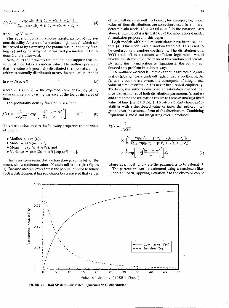
Ben-Akiva et al.

P(ijv) = Jexp{µ[c; + WY;1

+ v(t; + 'Y'Z;!]} ~j=t exp{µ[cj + ~ Yj + v(tj + 'Y Z)]}

where exp{x} = ex.

(4)

This equation contains a linear transformation of the sys­tematic utility function of a standard logit model, which can be arrived at by estimating the parameters in the utility func­tion (1) and calculating the normalized parameters in Equa­tions 2 and 3 afterward.

Now, relax the previous assumption, and suppose that the value of time takes a random value. The authors postulate that the value is lognormally distributed (i.e., its natural log­arithm is normally distributed) across the population, that is:

ln v - N(w, cr 2) (5)

where w is E(ln v) the expected value of the log of the value of time and cr2 is the variance of the log of the value of time.

The probability density function of v is then:

[ ( )2] 1 1 Inv - w f(v) = -- ·exp --

crvv'27T 2 er v>O (6)

This distribution implies the following properties for the value of time v:

•Median = exp (w), •Mode = exp (w - cr2),

•Mean = exp (w + cr2/2), and • Variance = exp (2w + cr2

) [exp ( cr2) - 1].

This is an asymmetric distribution skewed to the left of the mean, with a minimum value of 0 and a tail to the right (Figure 1). Because inc6me levels across the population tend to follow such a distribution, it has sometimes been asserted that values

£ ..0 0

..0 0 .._ a.

r I\

0.75 I \ I

(1) 0.50 .::: 0 I

:::J

E :::J u

0.25

\

I

89

of time will do so as well. In France, for example, lognormal value of time distributions are sometimes used in a binary, deterministic model (J = 2 and E; = 0 in the notation used above). This model is a special case of the more general model formulation proposed in this paper.

Logit models with random coefficients have been used be­fore (4). Our model uses a random trade-off. This is not to be confused with random coefficients. The distribution of a VOT trade-off in a i;:andom coefficient logit model would involve a distribution of the ratio of two random coefficients. By using the normalization in Equation 3, the authors ad­dressed this problem in a direct way.

The authors' method is unique in that it assumes a lognor­mal distribution for a trade-off rather than a coefficient. As far as the authors are aware, the assumption of a.lognormal value of time distribution has never been tested empirically. To do so, the authors developed an estimation method that provided estimates of both distribution parameters (wand er) and compared the estimation results to those assuming a fixed value of time (standard logit). To calculate logit choice prob­abilities with a distributed value of time, the authors inte­grated over the assumed form of the distribution. Combining Equations 4 and 6 and integrating over v produces:

P(i) 1

loo exp{µ[c; + WY; + v(t; + )' 1Z;)]} x o If=i exp{µ[cj + WYj + v(tj + )' 1Zj)]}

1 [ 1 (ln v - w) 2] x ; exp -2 er dv (7)

where µ, w, er, ~. and 'Y are the parameters to be estimated. The parameters can be estimated using a maximum like­

lihood approach, applying Equation 7 to the observed choice

---

Cumulative: F(v) Density: f(v)

------0.00 ........ __._ ......... __._ .................. L.....l-_._..._._........_.L-L.._._,.._._~ .......... _._.._J__._..._._...&-.JL-.&--'-'-&....L....l-i... .......... _,_-~-__._-~-.-....1--~-....._.-~-L....J

0 5 10 .15 20 25 30 35

Value of time: v (1988 fl/hour)

FIGURE 1 Rail SP data-estimated lognormal VOT distribution.

40 45 50

90

of each individual and maximizing the sum of the logged probabilities across the sample. The log-likelihood function was programmed using the Gauss statistical programming en­vironment. To reduce the computation time required, three extra steps were carried out:

1. A standard logit estimation procedure was first used to ' provide efficient starting values for the parameters.

2. The analytic first derivatives of the likelihood function were obtained and incorporated into the program.

3. A simple change of variable from (ln - w )/( cr\/2) to y was performed so that a Gauss-Hermite quadrature could be used to compute the integral very efficiently.

(The Gauss-Hermite quadrature is especially designed to eval­uate an unbounded integral of the form

Only a few quadrature points are required for high precision). After this latter transformation, Equation 7 can be rewritten as:

P(i) = roo exp{µ[cj + j3'Y; + exp(y\/2cr + w)(ti + -y'ZJ]}

x If=t exp{µ[cj + j3'Yj + exp(yv'2cr + w)(tj + -y'Zi)]}

1 x - exp( - y2 )dy v:rr (8)

Computation over 8 to 12 quadrature points generally pro­duces accurate results. The Gauss estimation routine was first tested on simulated data generated from a model specification based on a lognormally distributed value of time coefficient. The results were very satisfactory for both binary and poly­tomous choice settings. By generating very large samples, the authors could verify that the true value of each coefficient was retrieved. This ensures that the maximum likelihood pro­cedure produces consistent estimators. The type of results obtained using data from actual choices is discussed in Case Study Results. To allow a lognormally distributed value of time, a special submode! that coincides with the deterministic binary choice model needs to be introduced.

SUBMODEL

Suppose that µ ~ - oo. This corresponds to a deterministic choice framework, which is often used to model route choices or to develop traffic assignment procedures, and coincides with a framework that minimizes the generalized cost of trav­eling. This is an interesting special case that applies to any choice model that may be particularly useful for evaluating the share and the revenue from a toll road. Let us say that only Alternative 1 involves a toll and that the other alter­natives are free. In the authors' notation, one can formalize

TRANSPORTATION RESEARCH RECORD 1413

the problem as

P(ilv) = l{i = argmin[cj + j3'Yj + v(tj + -y' Z)]} j

i = 1, ... 'J (9)

where l(a) is an indicator function equal to 1 if a is true and 0 otherwise. Because Alternative 1 is the only alternative involving a monetary cost and all other alternatives are free, the authors assume that Yj = 0 and cj = 0 for all i -::/= l. This sets the cost composite of all free roads to zero. Let j denote the best free alternative:

j = argmin(ti + -y' Z) (10) j4' 1

The random VOT framework can be used to model the choice between the toll road and the best free alternative. The choice probability of the costly alternative can be expressed as

P(l) = prob[c1 + ~'Y1 + v(t1 + -y' Z 1) :5 v(t; + -y' Z;)]

= prob[v(at + -y' az) ~ c1 + 13'Yi)

( C1 + J3'Y1)

P(l) = prob v;;:::: !lt + -y' !lZ

[ ( C1 + f3'Y1)] = prob Inv ;;:::: In !lt + -y' !lZ

{Inv - w 1 [ ( c1 + 13'Y1 ) ] } =prob ---;;::::- In - w

cr cr !lt + -y' az

(11)

(12)

Because it is assumed that ln v is normally distributed, the following equation can finally be written:

{ 1 [ ( C1 + 13'Y1)]} P(l) = <I> ~ w - ln !!:,.t + "Y, !!:,.Z (13)

where <I> denotes the standard normal cumulative distribution function. This model formulation corresponds to a binary nonlinear probit model of the choice between the best free alternative and the nonfree alternative.

CASE STUDY RESULTS

Intercity Rail SP Data

In 1987, the Hague Consulting Group conducted a study for the Nederlandse Spoorwegen (NS) on the potential for sub­stitution between car and rajl for intercity travel as a function of rail service levels and fares (5). The sample was composed of 235 individuals who had recently traveled by car or rail from the Dutch city of Nijmegen, which is near the German border, to Amsterdam, Rotterdam, or Den Haag, all of which are located about 125 km west. A computer-based home in­terview was used. Each respondent gave a detailed account of his or her actual journey, including all travel costs, times, and interchanges. The respondent was then asked for his or

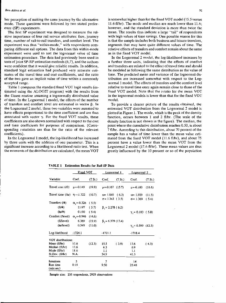
Ben-Akiva et al.

her perception of making the same journey by the alternative mode. These questions were followed by two stated prefer­ence (SP) experiments.

The first SP experiment was designed to measure the rel­ative importance of four rail service attributes: fare, journey time, number of rail-to-rail transfers, and comfort level. The experiment was thus "within-mode,'' with respondents com­paring different rail options. The data from this within-mode experiment were used to test the lognormal value of time estimation procedure. The data had previously been used in tests of joint SP-RP estimation methods (6,7), and the authors were confident that it would give reliable results. In addition, standard logit estimation had produced very accurate esti­mates of the travel time and cost coefficients, and the ratio of the two gave an implicit value of time within a commonly accepted range.

Table 1 compares the standard fixed VOT logit results (es­t~mated using the ALOGIT program) with the results from the Gauss routine assuming a lognormally distributed value of time. In the Lognormal 1 model, the effects of the number of transfers and comfort level are estimated in vector J3. In the Lognormal 2 model, these two variables were assumed to have effects proportional to the time coefficient and are thus associated with vector 'Y· For the fixed VOT results, these coefficients are also shown normalized with respect to the cost and time coefficients for purposes of comparison. (Corre­sponding t-statistics are thus for the ratio of the relevant coefficients).

In the Lognormal 1 model, the log-likelihood has increased by three units with the addition of one parameter. This is a significant increase according to a likelihood ratio test. When the moments of the distribution are calculated, the mean VOT

91

is somewhat higher than for the fixed VOT model (15.5 versus 11.6 fl/hr). The mode and median are much lower than 11.6; however, and the standard deviation is more than twice the mean. The results thus indicate a large "tail" of respondents with high values of time savings. One possible reason for this is that the sample includes both business and leisure travelers, segments that may have quite different values of time. The relative effects of transfers and comfort remain about the same as in the fixed VOT model.

In the Lognormal 2 model, the log-likelihood increases by a further three units, indicating that the effects of comfort and transfers are related to the effect of travel time and should be modeled as following the same distribution as the value of time. The predicted mean and variance of the lognormal dis­tribution are increased somewhat with respect to the Log­normal 1 model. The effects of transfers and the comfort level relative to travel time once again remain close to those of the fixed VOT model. Note that the t-ratio for the mean VOT in the lognormal models is lower than that for the fixed VOT model.

To provide a clearer picture of the results obtained, the estimated VOT distribution from the Lognormal 2 model is plotted in Figure 1. The mode, which is the peak of the density function, occurs between 1 and 2 fl/hr. (The scale of the density function is not shown in the figure). The median, the point where the cumulative distribution reaches 0.50, is about 7 fl/hr. According to this distribution, about 70 percent of the sample has a value· of time lower than the mean value esti­mated from the fixed VOT model (11.6 fl/hr), and about 75 percent have a value lower than the mean VOT from the Lognormal 2 model (17.6 fl/hr). These mean values are thus greatly influenced by the 10 percent or so of the population

TABLE 1 Estimation Results for Rail SP Data

Fixed VOT Lognormal I Lognormal 2

Variable: Coef. (T.St.) Coef. (T.St.) Coef. (T.St.)

Travel cost (/fl) µ=-0.149 (19.9) µ=-0.167 (15.7) µ=-0.180 (16.6)

Travel time (/hr) Tl =-1.722 (10.7) CO= 1.840 ( 6.3) CO= 1.929 (11.5)

O'= 1.343 ( 3.5) O'= 1.369 ( 5.4) Transfers (/#) ex, =-0.326 ( 5.5)

(fl/#) 2.197 ( 5.7) ~,= 2.278 ( 6.2)

(hr/#) 0.190 ( 5.4) Y1= 0.183 ( 5.8)

Comfort (nevel) CX2=-0.946 (14.6)

(fl/level) 6.369 (15.9) ~2= 6.379 (17.4) (hr/level) 0.549 (11.0) Y2= 0.599 (12.5)

Log-likelihood -1724.l -1721.1 -1718.4

VOT distributions: Mean (fl/hr) 11.6 (12.3) 15.5 ( 3.9) 17.6 ( 4.3) Median (fl/hr) 11.6 6.3 6.9 Mode (fl/hr) 11.6 1.1 1.1 St.Dev. (fl/hr) N.A. 34.9 41.3

Iterations 5 7 14 Run time 0:19 9:50 25:48 (min: sec)

Sample size: 235 respondents, 2929 observations

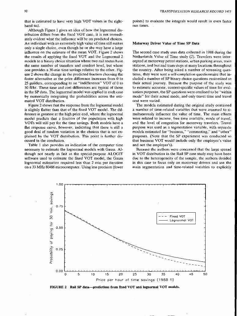
92

that is estimated to have very high VOT values in the right­hand tail.

Although Figure 1 gives an idea of how the lognormal dis­tribution differs from the fixed VOT case, it is not immedi­ately evident what the influence will be on predicted choices. An individual with an extremely high value of time still makes only a single choice, even though he or she may have a large influence on the estimate of the mean VOT. Figure 2 shows the results of applying the fixed VOT and the Lognormal 2 models to a binary choice situation where two rail routes have the same number of transfers and comfort level, but where one provides a 30-min time savings relative to the other. Fig­ure 2 shows the change in the predicted fraction choosing the faster alternative as the price difference increases from 0 to 25 guilders, corresponding to an "indifference" VOT of 0 to 50 fl/hr. These time and cost differences are typical of those in the SP data. The lognormal model was applied in each case by numerically integrating the probabilities across the esti­mated VOT distribution.

Figure 2 shows that the response from the lognormal model is slightly flatter than that of the fixed VOT model. The dif­ference is greatest at the high price end, where the lognormal model predicts that a fraction of the population with high VOTs will still pay for the time savings. Both models have a flat response curve, however, indicating that there is still a good deal of random variation in the choices that is not ex­plained by the VOT distribution. This point is further dis­cussed in the conclusion.

Table 1 also provides an indication of the computer time necessary to estimate the lognormal models with Gauss. Al­though not nearly as fast as the special-purpose ALOGIT software used to estimate the fixed VOT model, the Gauss lognormal estimation required less than 2 min per iteration on a 33 MHz 80486 microcomputer. Using less precision (fewer

1.00

en O'l c

·:;: 0 en

0.75 c '§

0 l"'1

I...

2 O'l

0.50 c

·:;._ 0 a.

0

.£ 0.25 15 0

..0 0 I...

0....

TRANSPORTATION RESEARCH RECORD 1413

points) to evaluate the integrals would result in even faster run times.

Motorway Driver Value of Time SP Data

The second case study uses data collected in 1988 during the Netherlands Value of Time study (2). Travelers were inter­cepted at motorway petrol stations, urban parking areas, train stations, and bus and tram stops at many locations throughout the country. After being asked a number of screening ques­tions, they were sent a self-completion questionnaire that in­cluded a number of SP binary choice questions customized to their actual journey. Because the purpose of the study was to estimate accurate, context-specific values of time for eval­uation purposes, the SP questions were confined to be "within mode" for their actual mode, and only travel time and travel cost were varied.

The models estimated during the original study contained a number of time-related variables that were assumed to si­multaneously influence the value of time. The main effects were related to income, free time available, mode of travel, and the level of congestion for motorway travelers. Travel purpose was used as a segmentation variable, with separate models estimated for "business," "commuting," and "other" purposes. (Note that the SP experiment was conducted so that business VOT would include only the employee's value and not the employer's).

Because the authors were concerned that the large spread in VOT distribution in the Rail SP case study may have been due to the heterogeneity of the sample, the authors decided in this case to focus only on motorway drivers and use the main segmentation and time-related variables to explicitly

Fixed VOT Lognormol VOT

0.00 ........ ......._ ......... _._..._. ........................... ...._ ....... ......._ .......... ......._ ......... _._ ........ _._..._. ........................... ...._ .......... _.._ ........ _._..._. .......... ....._._._ ..................................... _ 0 5 10 15 20 25 30 35 40 45 50

Price per hour of time savings ( 1988 fl)

FIGURE 2 Rail SP data-predictions from fixed VOT and lognormal VOT models.

Ben-Akiva et al.

account for many of the person and trip characteristics ex­pected to influence the value of time savings.

Table 2 contains results for fixed VOT and lognormal VOT models for all three segments, using extra travel time variables as functions of income level, number of car passengers, amount of free time available (discretionary time as deduced from self-reported time budgets), and congestion level. The conges­tion level is the percentage at which the observed traffic speed at the time of intercept was below 120 km/hr. Continuous traffic speed and flow monitors were located near the intercept sites. The extra travel time variables are interaction terms with the base travel time variable and thus by definition are proportionally related to the value of time. They were thus associated with the 'Y parameters.

For both the fixed VOT and the lognormal VOT models in Table 2, the overall results agree with those of the original study: business and commuting values are higher than those for other purposes, and values markedly increase with income level and decrease with available free time. The effects of congestion and car occupancy are less significant, with the signs varying across the segments.

The most striking results in Table 2 are the huge improve­ments in the lognormal models relative to the fixed VOT models-70 likelihood units or more with the addition of one parameter for all three segments. This improvement is much greater than in the first case study, suggesting that the log-

93

normal distribution is also appropriate after one has already accounted for as many important observable factors influ­encing VOT as possible. In contrast to the first case study, the mean VOTs for the lognormal models have t-ratios just as high as for the fixed VOT estimates.

For business and commuting, the mean VOT increases by a factor of more than two in the lognormal models relative to the fixed VOT models. The median VOT is also greater than the estimate from the fixed VOT model. For other pur­poses, the increase is somewhat less. The lognormal standard deviation is about 1.5 times the mean for all three segments. Note that the proportional effect of income is about one-third less in the lognormal VOT models than for the fixed VOT models for business and commuting. This result suggests that what had been identified as an income effect in the simpler models may be partially due to the correlation of income to other unobserved influences on VOT. The congestion effects also tend to become smaller in the lognormal models.

The lognormal density and cumulative functions for the three segments are shown in Figure 3. The large tails in the distribution for business and commuting at the high-VOT end are evident. Note that the distributions in Figure 3 (and at the bottom of Table 2) are for the "base" VOT only and do not yet include the extra effects of income. When those effects are added, the differences among the segments become more pronounced, as is shown in Figure 4.

TABLE 2 Estimation Results for Motorway VOT SP Data

Segment: Business Commuting Others Respondents: 332 218 287 Observations: 3984 2616 3444

Fixed VOT Coef. (T.St.) Coef. (T.St.) Coef. (T.St.)

Travel cost (/fl) µ = -0.319 (17.5) -0.496 (15.9) -0.520 (22.2)

Travel time (/hr)11 = -5.026 ( 6.9) -8.009 ( 6.7) -5.802 ( 9.0) Time-related effects: cx/11 = Passengers (/#) + 9.8% ( 1.9) +I.5% ( 0.3) -5.7% ( 3.7) Income (/Kfl/mth) +10.2% ( 4.2) +4.1% ( 2.6) +6.9% ( 4.9) Free Time (/hr/day) - 8.2% ( 9.7) - 6.0% ( 7.0) -2.8% ( 5.0) Congestion (/% delay) + 1.3% ( 2.3) +J.1% ( 2.2) -1.7% ( 3.0)

Log-likelihood -1992.l -1359.2 -1855.0

Lognormal VOT Coef. (T.St.) Coef. (T.St.) Coef. (T.St.)

Travel cost (/fl)µ= -0.351 ( 3.0) -0.532 ( 2.5) -0.483 ( 3.2)

Travel time (/hr) ro= 3.146 (32.6) 2.995 (27.4) 2.184 (20.3)

CJ= 1.110 (25.2) 1.080 (24.0) 1.055 (27.1) Time-related effects: y = Passengers (/#) + 9.1% ( 2.4) -0.2% ( 0.5) -4.2% ( 2.6) Income (/Kfl/mth) + 6.2% ( 4.8) +2.7% ( 2.5) +8.7% ( 5.1) Free Time (/hr/day) - 8.0% (18.2) - 6.4% (13.5) -2.2% ( 3.5) Congestion (/% delay) + 0.0% ( 0.2) +0.7% ( 2.0) -1.3% ( 3.5)

Log-likelihood -1846.5 -1286.8 -1740.2

Fixed VOT (fl/hr) 15.8 ( 7.0) 16.1 ( 6.9) 11.2 ( 9.5) Lognormal VOT: Mean (fl/hr) 42.8 ( 8.3) 35.8 ( 8.3) 15.5 ( 8.8) Median (fl/hr) 23.2 20.0 8.9 Mode (fl/hr) 6.8 6.2 2.9 St.Dev. (fl/hr) 66.0 53.2 22.2

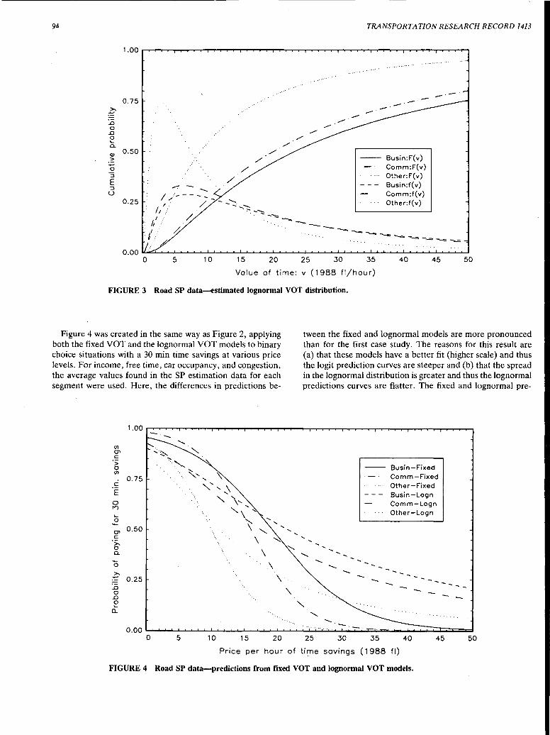
94

£ ..0 0

..0 0 ,_ Q.

Q)

-~ 0 :l

E :l u

TRANSPORTATION RESEARCH RECORD 1413

1.00 ...................... .._ __ .................... ...-,....,......,..,....,.....,........-T._....,..... ....... .,....._....,....,,....,...._ ................................... -.-...................... ,_,....,....,,_,..~

0.75

0.50

.,,,.... - -0.25

I _ .. _ - - - -/-: / - - -"::::. -

/1 .... ...... :-. -""'::::: ---/,/ / /, ---

: /: ~ #

.. ·····.

. . . . . . . . . . . . . . . '

.-

Busin:F(v) Comm:F(v) Other:F(v) Busin:f(v) Comm:f(v) Other:f(v)

---....... ""'""- ---acr ---= --== ---== ---== ---= -

o.oo~::;i._ ........... -1-........... _._ ................. .....___ ......... _._ ........... -4-.i......L_._.&.....1._._..i........i_,_ ..................... .....___ ......... _._ ........... _._ ........... _,__,__,_,_..&......IL.....L.~ ......... ~ 0 5 10 15 20 25 30 35

Value of time: v (1988 fl/hour)

40 45 50

FIGURE 3 Road SP data-estimated lognormal VOT distribution.

Figure 4 was created in the same way as Figure 2, applying both the fixed VOT and the lognormal VOT models to binary choice situations with a 30 min time savings at various price levels. For income, free time, car occupancy, and congestion, the average values found in the SP estimation data for each segment were used. Here, the differences in predictions be-

tween the fixed and lognormal models are more pronounced than for the first case study. The reasons for this result are (a) that these models have a better fit (higher scale) and thus the logit prediction curves are steeper and (b) that the spread in the lognormal distribution is greater and thus the lognormal predictions curves are flatter. The fixed and lognormal pre-

1.0o,.....,. ....... 'T"""'l'..,....,.....,...,......-,....,..-,-....... ....,..'T"""'l'...,........,...,....,.....,...,.........., ...... .......,,....,......,.. ..................... -r-....... -.-............. ...-....... .._ ....... _

0.75

,_ .E 0\ 0.50 c

·:;., 0 Q.

0

£ 0.25 :0 0

..0 0 ,_

0...

..... ~ .......... ~

. "'-', \ ' " \, "\' ~ ~ ',

'-.. \ ~

\ ···.\

\·

Busin-Fixed Comm-Fixed Other-Fixed Busin-Logn Comm-Logn Other-Logn

o.ooL.i..~_._..1......1......i....L....1......1.......i-"-"'--1._.__L....1...~--L..."'--l.....L....,j~~.;;.i..;...i.....;L;......:i~J:::.1.;...z=.__.......i-..._.::::i:::c:::i::::::c:::i::=:::1

0 5 10 15 20 25 30 35 40

Price per hour of tir::ne savings ( 1988 fl)

FIGURE 4 Road SP data-predictions from fixed VOT and lognormal VOT models.

45 50

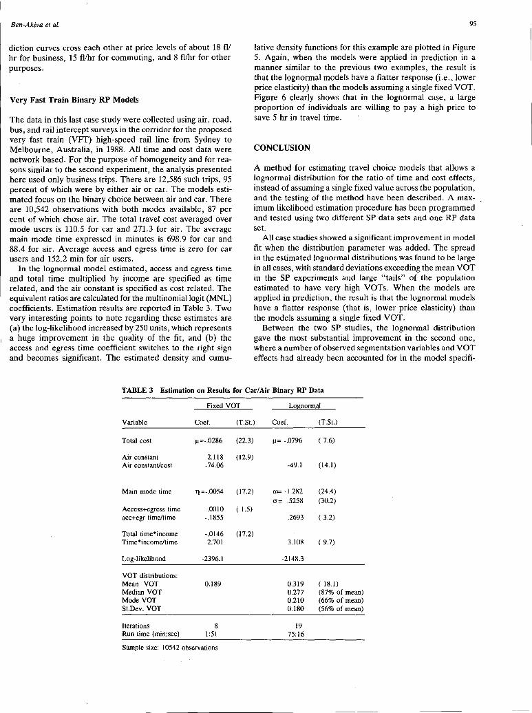
Ben-Akiva et al.

diction curves cross each other at price levels of about 18 fl/ hr for business, 15 fl/hr for commuting, and 8 fl/hr for other purposes.

Very Fast Train Binary RP Models

The data in this last case study were collected using air, road, bus, and rail intercept surveys in the corridor for the proposed very fast train (VFT) high-speed rail line from Sydney to Melbourne, Australia, in 1988. All time and cost data were network based. For the purpose of homogeneity and for rea­sons similar to the second experiment, the analysis presented here used only business trips. There are 12,586 such trips, 95 percent of which were by either air or car. The models esti­mated focus on the binary choice between air and car. There are 10,542 observations with both modes available, 87 per cent of which chose air. The total travel cost averaged over mode users is 110.5 for car and 271.3 for air. The average main mode time expressed in minutes is 698.9 for car and 88.4 for air. Average access and egress time is zero for car users and 152.2 min for air users.

In the lognormal model estimated, access and egress time and total time multiplied by income are specified as ·time related, and the air constant is specified as cost related. The equivalent ratios are calculated for the multinomial logit (MNL) coefficients. Estimation results are reported in Table 3. Two very interesting points to note regarding these estimates are (a) the log-likelihood increased by 250 units, which represents a huge improvement in the quality of the fit, and (b) the access and egress time coefficient switches to the right sign and becomes significant. The estimated density and cumu-

95

lative density functions for this example are plotted in Figure 5. Again, when the models were applied in prediction in a manner similar to the previous two examples, the result is that the lognormal models have a flatter response (i.e., lower price elasticity) than the models assuming a single fixed VOT. Figure 6 clearly shows that in the lognormal case, a large proportion of individuals are willing to pay a high price to save 5 hr in travel time.

CONCLUSION

A method for estimating travel choice models that allows a lognormal distribution for the ratio of time and cost effects, instead of assuming a single fixed value across the population, and the testing of the method have been described. A max­imum likelihood estimation procedure has been programmed and tested using two different SP data sets and one RP data set.

All case studies showed a significant improvement in model fit when the distribution parameter was added. The spread in the estimated lognormal distributions was found to be large in all cases, with standard deviations exceeding the mean VOT in the SP experiments and large "tails" of the population estimated to have very high VOTs. When the models are applied in prediction, the result is that the lognormal models have a flatter response (that is, lower price elasticity) than the models assuming a single fixed VOT.

Between the two SP studies, the lognormal distribution gave the most substantial improvement in the second one, where a number of observed segmentation variables and VOT effects had already been accounted for in the model specifi-

TABLE 3 Estimation on Results for Car/ Air Binary RP Data

Fixed VOT Log normal

Variable Coef. (T.St.) Coef. (T.St.)

Total cost µ=-.0286 (22.3) µ= -.0796 ( 7.6)

Air constant 2.118 (12.9) Air constant/cost -74.06 -49.1 (14.1)

Main mode time Tl =-.0054 (17.2) c.o= -1.282 (24.4)

CJ= .5258 (30.2) Access+egress time .0010 ( 1.5) acc+egr time/time -.1855 .2693 ( 3.2)

Total time*income -.0146 (17.2) Time*income/time 2.701 3.108 ( 9.7)

Log-likelihood -2396.l -2148.3

VOT distributions: Mean VOT 0.189 0.319 ( 18.1) Median VOT 0.277 (87% of mean) Mode VOT 0.210 (66% of mean) St.Dev. VOT 0.180 (56% of mean)

Iterations 8 19 Run time (min:sec) 1:51 75:16

Sample size: 10542 observations

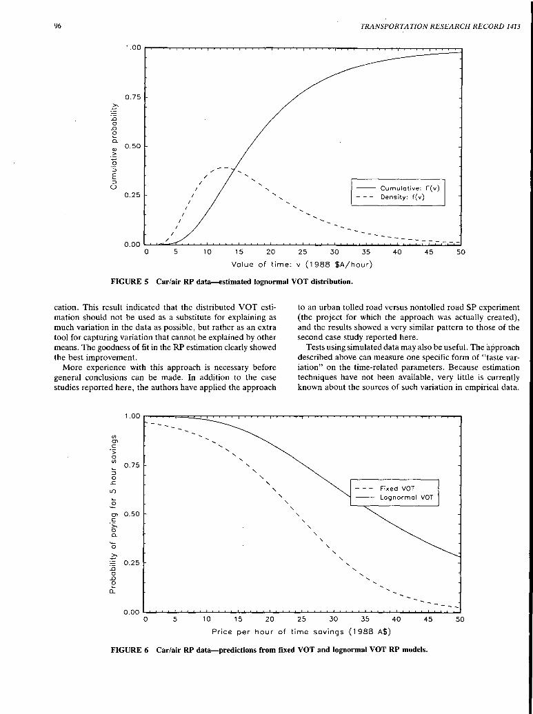
96 TRANSPORTATION RESEARCH RECORD 1413

0.75 ~

:.0 0

.D

~ 0...

(I) 0.50

>

0 :J /

E / :J I

' u I ' Cumulative: F(v) 0.25 I ' Density: f( v)

I I

---0 5 10 15 20 25 30 35 40 45 50

Value of time: v ( 1988 $A/hour)

FIGURE 5 Car/air RP data-estimated lognormal VOT distribution.

cation. This result indicated that the distributed VOT esti­mation should not be used as a substitute for explaining as much variation in the data as possible, but rather as an extra tool for capturing variation that cannot be explained by other means. The goodness of fit in the RP estimation clearly showed the best improvement.

More experience with this approach is necessary before general conclusions can be made. In addition to the case studies reported here, the authors have applied the approach

Ul cr> c

·:;: 0 Ul

..... :J 0 ..c

L.<1 ..... .E cr> c

·:;:., 0 0.

0 ~

.D 0

.D

~ 0...

0.75 '

0.50

0.25

0.00

' ' ' ' ' ' '

to an urban tolled road versus nontolled road SP experiment (the project for which the approach was actually created), and the results showed a very similar pattern to those of the second case study reported here.

Tests using simulated data may also be useful. The approach described above can measure one specific form of "taste var­iation" on the time-related parameters. Because estimation techniques have not been available, very little is currently known about the sources of such variation in empirical data.

' ' ' '

Fixed VOT Lognormol VOT

---0 5 10 15 20 25 30 35 40 45 50

Price per hour of time savings ( 1988 A$)

FIGURE 6 Car/air RP data-predictions from fixed VOT and lognormal VOT RP models.

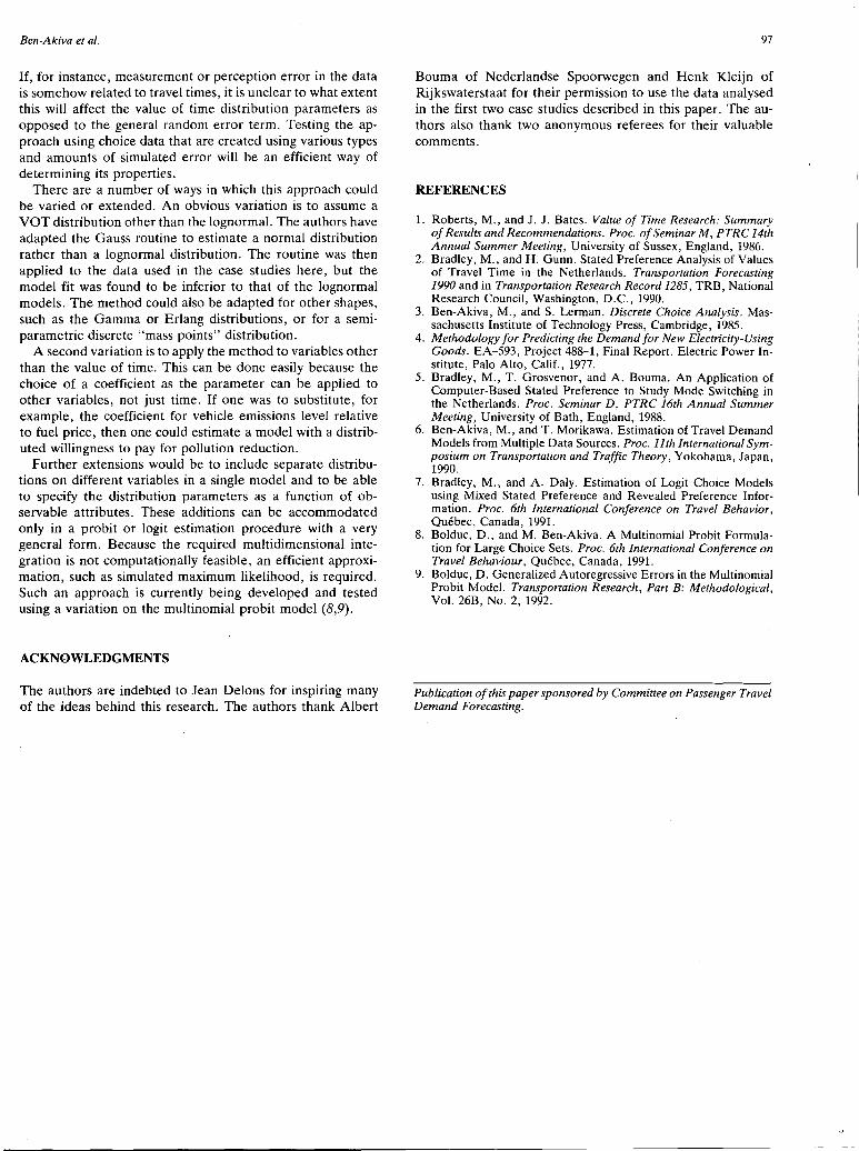
Ben-Akiva et al.

If, for instance, measurement or perception error in the data is somehow related to travel times, it is unclear to what extent this will affect the value of time distribution parameters as opposed to the general random error term. Testing the ap­proach using choice data that are created using various types and amounts of simulated error will be an efficient way of determining its properties.

There are a number of ways in which this approach could be varied or extended. An obvious variation is to assume a VOT distribution other than the lognormal. The authors have adapted the Gauss routine to estimate a normal distribution rather than a lognormal distribution. The routine was then applied to the data used in the case studies here, but the model fit was found to be inferior to that of the lognormal models. The method could also be adapted for other shapes, such as the Gamma or Erlang distributions, or for a semi­parametric discrete "mass points" distribution.

A second variation is to apply the method to variables other than the value of time. This can be done easily because the choice of a coefficient as the parameter can be applied to other variables, not just time. If one was to substitute, for example, the coefficient for vehicle emissions level relative to fuel price, then one could estimate a model with a distrib­uted willingness to pay for pollution reduction.

Further extensions would be to include separate distribu­tions on different variables in a single model and to be able to specify the distribution parameters as a function of ob­servable attributes. These additions can be accommodated only in a probit or logit estimation procedure with a very general form. Because the required multidimensional inte­gration is not computationally feasible, an efficient approxi­mation, such as simulated maximum likelihood, is required. Such an approach is currently being developed and tested using a variation on the multinomial probit model (8,9).

ACKNOWLEDGMENTS

The authors are indebted to Jean Delons for inspiring many of the ideas behind this research. The authors thank Albert

97

Bouma of Nederlandse Spoorwegen and Henk Kleijn of Rijkswaterstaat for their permission to use the data analysed in the· first two case studies described in this paper. The au­thors also thank two anonymous referees for their valuable comments.

REFERENCES

1. Roberts, M., and J. J. Bates. Value of Time Research: Summary of Results and Recommendations. Proc. of Seminar M, PTRC 14th Annual Summer Meeting, University of Sussex, England, 1986.

2. Bradley, M., and H. Gunn. Stated Preference Analysis of Values of Travel Time in the Netherlands. Transportation Forecasting 1990 and in Transportation Research Record 1285, TRB, National Research Council, Washington, D.C., 1990.

3. Ben-Akiva, M., and S. Lerman. Discrete Choice Analysis. Mas­sachusetts Institute of Technology Press, Cambridge, 1985.

4. Methodology for Predicting the Demand for New Electricity-Using Goods. EA-593, Project 488-1, Final Report. Electric Power In­stitute, Palo Alto, Calif., 1977.

5. Bradley, M., T. Grosvenor, and A. Bouma. An Application of Computer-Based Stated Preference to Study Mode Switching in the Netherlands. Proc. Seminar D, PTRC 16th Annual Summer Meeting, University of Bath, England, 1988.

6. Ben-Akiva, M., and T. Morikawa. Estimation of Travel Demand Models from Multiple Data Sources. Proc. 11th International Sym­posium on Transportation and Traffic Theory, Yokohama, Japan, 1990.

7. Bradley, M., and A. Daly. Estimation of Logit Choice Models using Mixed Stated Preference and Revealed Preference Infor­mation. Proc. 6th International Conference on Travel Behavior, Quebec, Canada, 1991.

8. Bolduc, D., and M. Ben-Akiva. A Multinomial Probit Formula­tion for Large Choice Sets. Proc. 6th International Conference on Travel Behaviour, Quebec, Canada, 1991.

9. Bolduc, D. Generalized Autoregressive Errors in the Multinomial Probit Model. Transportation Research, Part B: Methodological, Vol. 26B, No. 2, 1992.

Publication of this paper sponsored by Committee on Passenger Travel Demand Forecasting.

98 TRANSPORTATION RESEARCH RECORD 1413

Application and Interpretation of Nested Logit Models of Intercity Mode Choice CHRISTOPHER v. FORINASH AND FRANKS. KOPPELMAN

A clear un.derstanding of the sources and amount of ridership on a ne~ or improved travel mode is critical to evaluating the fi­nancial, travel flow, and external impacts of proposed improve­ments. The multinomial logit model traditionally used to model intercity mode choice may not adequately reflect traveler behav­ior because it restricts the relative probability of choosing between any pair of existing modes to be unchanged when other modes are introduced or changed. The nested logit model provides a computati~nally feasible generalization to the multinomial logit model, which allows for specified mode pairs to exhibit increased sensitivity to changes in service. Full information estimation of nested l~git models allows efficient use of information and yields results duectly comparable to multinomial logit models. Business travel in the Ontario-Quebec corridor of Canada is examined. A set of nested logit structures that allow for various combinations of ~ifferential sensitivity to changes in service quality of rail is estimated. Nested logit structures with bus-train or car-train nests prove superior to the multinomial logit model. Both of the nested logit models predict larger increases in rail shares than the mul­tinomial logit model in response to rail service improvements, but the source of that increased ridership differs between the nested logit structures. This points to the need for models of individual choice that retain the advantages of nested logit while allowing pairwise similarity between alternatives.

Congestion in intercity travel increases the cost of travel di­rectly through the loss of traveler time and indirectly through increased costs in system operation. These costs are trans­ferred to travelers and others by common carriers through fares and by governments through taxes or debt. Considerable attention has been directed toward rapidly increasing conges­tion during the last decade and projections of substantial ad­ditional increases through the next two decades (1,2). Pro­posals to alleviate existing and projected congestion include construction of new airports (3-5); construction or widening of express highways, some with toll charges ( 6-8); upgrading of conventional rail services (9 ,10) and construction of new high-speed ground transportation based on rail or magnetic levitation technology (11). It has been difficult to implement many of these proposals because of concerns about financing and environmental impacts and differences among govern­mental and private institutions. The difficulty reaching posi­tive implementation decisions for both new airport and high­speed ground transportation alternatives may, in part, be due to concerns about the quality of ridership and revenue forecasts.

A fundamental issue in the prediction of ridership is the ability to model and explain the likely projected changes in ridership and the sources of projected ridership. A clear rep-

The Transportation Center, 1936 Sheridan Road, Evanston, Ill. 60208.

resentation of the sources of new ridership on new or im­proved alternatives can increase the confidence of both public and private investors in the likelihood of recovering their investment. It can also be used to scale the beneficial effect of the investment on congestion and external impacts. This paper tests the application of the nested logit model to esti­mate ridership on intercity travel modes and compares the results of the nested logit model to the more commonly used multinomial logit model. The issue of predicting changes in total ridership in response to improvements in modal ser­vice is not addressed in this paper but has been addressed by others (12 ,13).

The multinomial logit model has been used almost exclu­sively to model both urban and intercity mode choice until recently (14,15). The multinomial logit model is widely used because its mathematical form is simpler than that of alter­native models, making it easier to estimate and interpret. However, the important disadvantage of the multinomial logit model is that it restricts the relative probability of choosing between any pair of unchanged modes to be unchanged due to changes in other modes of travel. This restriction implies that the introduction of any new mode or the improvement of any existing mode will affect all other modes proportion­ally. This property of equal proportional change or equal cross-elasticity of unchanged modes is unlikely to represent actual choice behavior in a variety of situations. Such mis­representation of choice behavior can result in incorrect es­timated models and incorrect predictions of mode share and diversion from existing modes. Differences in the impact of the introduction of new services on existing modes can be addressed by adoption of the multinomial probit model, which is rarely used in application due to problems of complexity, estimation, and interpretation, or the nested logit model.

Studies of intercity mode choice that have used the mul­tinomial logit model include the Ontario-Quebec corridor in Canada (12), Twin Cities-Duluth in Minnesota (16), and the United States as a whole (17-19). Although the nested logit model was recommended for "immediate implementation" at the 3rd International Conference on Behavioural Travel Modeling in 1977 (14), it use has been limited due, in part, to the limited availability of the more flexible software needed to estimate the nested logit model relative to the availability of a variety of software to estimate the multinomial logit model. The nested logit model has been used to estimate mode choice models for urban mode-choice and for multi­modal and multidimensional choices (20-23), although the older efforts were accomplished using inefficient two-stage limited-information maximum likelihood estimation. Hensher (15) recommended adoption of the nested logit model for inter-

Forinash and Koppelman

city mode choice estimation. However, there have been few applications of the nested logit model in the intercity mode choice context. These include the estimation of a multidi­mensional mode, destination, and rental-car choice model (24) and a nested mode and air-fare-class choice model (Kop­pelman, unpublished data), both using limited-information estimation.

NESTED LOGIT MODEL DESCRIPTION AND PROPERTIES

The nested logit and multinomial logit models can each be depicted by a tree structure that represents all the alternatives. The multinomial logit model treats all alternatives equally, whereas the nested logit model includes intermediate branches that group alternatives (Figure 1). The grouping of alterna­tives indicates the degree of sensitivity (cross-elasticity) among alternatives. Alternatives in a common nest show the same degree of increased sensitivity compared to alternatives not in the nest. Thus, although the nested logit model is not completely flexible in the sense that distinct pairwise sensi­tivities cannot be estimated, it provides a more general struc­ture than the multinomial logit model. The differences in structure can result in dramatically different mode ridership projections and diversions than those obtained by the mul­tinomial logit model in cases where the nested logit model is significantly different from the multinomial logit model.

The widely adopted paradigm of utility maximization pro­vides a link by which choice probabilities can be estimated given characteristics of the modes and the decision maker. This paradigm holds that an individual acts to maximize his or her utility by choosing among the available alternatives. Utility can then be estimated as a function of the traveler and mode characteristics. The choice probabilities can be com­puted as functions of the relative utilities among alternatives. Conventionally, the utility of an alternative, Uij• is assumed to be the sum of a deterministic component, V;j, which de­scribes the characteristics of individual i and the attributes of alternative j, and a random term, E;j, which represents ele­ments not measured or included in the model:

(1)

Further, the measured and included component of the model is represented by a linear additive function that includes pa­rameters, J3, and variables, X;j, which are predetermined func-

a.

b c

FIGURE 1 Example four-mode nested choice structure: modes a, b, c, and d.

99

tions of the characteristics of individual i and the attributes . of alternative j:

(2)

Assumptions about the distribution of the error terms E;j lead to different model structures.

The assumption that the error terms are distributed inde­pendently and identically over individuals and alternatives, with a Gumbel (0,1) distribution, yields the multinomial logit model (25 ,26):

esp(V;)

L exp(V;) j'<d

where J is the set of available alternatives.

(3)

The nested logit model is derived from an assumption tl!at some of the alternatives share common components in the random term. That is, the random term, ej, ignoring the in­dividual subscript for simplicity of notation, can be decom­posed into a portion associated with each alternative and a portion associated with groups of alternatives. For example, consider the nested model in Figure 1, where alternatives b, c, and dare included in the nest, which is labeled e. The total errors for alternatives b, c, and dare defined as eb + ee, ee + ee and ed + Ee. The total error for alternative a not in the nest is ea. The included and measured portion of utility may

·also be decomposed into two parts representing specific char-acteristics of the alternative, Vb, Ve, and Vd, and common characteristics of the nested alternatives, Ve. That is:

(4)

The nested logit model is obtained by assuming further that the error terms for each alternative-ea, eb + ee, Ee + Ee and ed + ee-are distributed Gumbel (0,1) and that the inde­pendent portion of the error terms for the nested alterna­tives-eb, ee anded-are distributed independent Gumbel (0,01

)

(25). The common error component, ee, for the nested alter­natives represents a covariance relationship that describes an increased similarity between pairs of nested alternatives and leads to a higher sensitivity (cross-elasticity) between alter­natives. If this common component, ee, is reduced to zero, the model reduces to the multinomial logit model with no covariance of error terms among the alternatives.

These assumptions yield the following conditional choice probability for each nested alternative n among the nested alternatives (conditional on choice of the nest at the higher level):

(5.1)

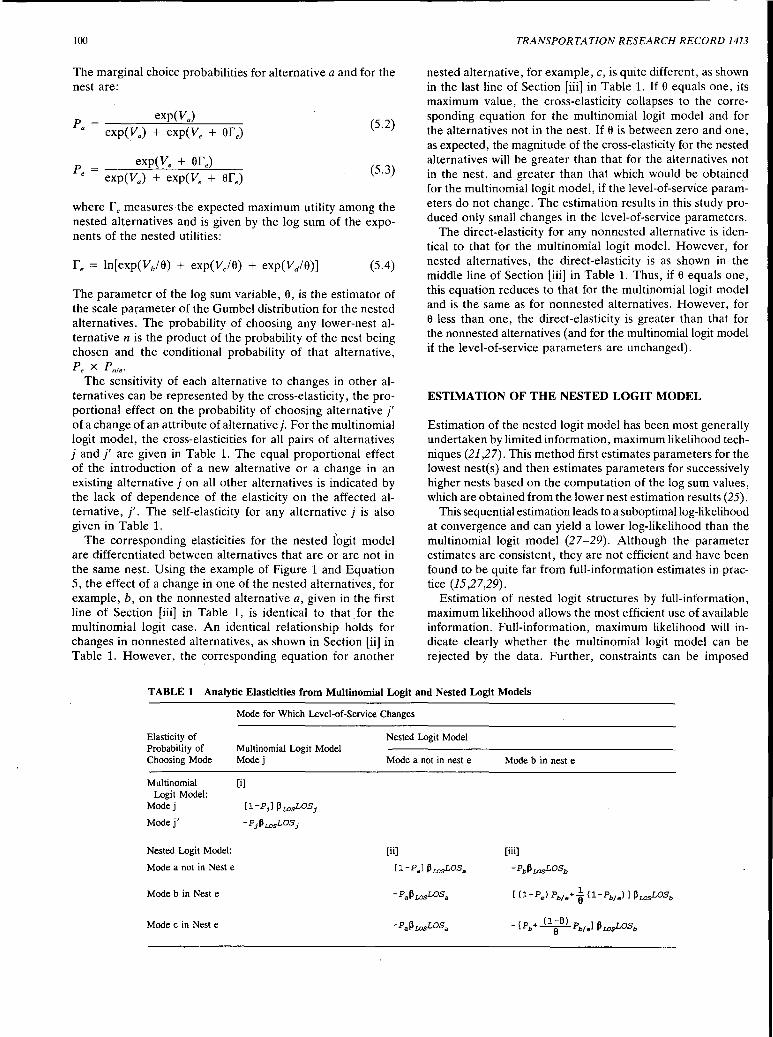
100

The marginal choice probabilities for alternative a and for the nest are:

(5.2)

p = exp( Ve + ere) e exp(Va) + exp(Ve + ere) (5.3)

where re measures the expected maximum utility among the nested alternatives and is given by the log sum of the expo­nents of the nested utilities:

The parameter of the log sum variable, e, is the estimator of the scale parameter of the Gumbel distribution for the nested alternatives. The probability of choosing any lower-nest al­ternative n is the product of the probability of the nest being chosen and the conditional probability of that alternative, Pe X pn/e•

The sensitivity of each alternative to changes in other al­ternatives can be represented by the cross-elasticity, the pro­portional effect on the probability of choosing alternative j' of a change of an attribute of alternative j. For the multinomial logit model, the cross-elasticities for all pairs of alternatives j and j' are given in Table 1. The equal proportional effect of the introduction of a new alternative or a change in an existing alternative j on all other alternatives is indicated by the lack of dependence of the elasticity on the affected al­ternative, j'. The self-elasticity for any alternative j is also given in Table 1.

The corresponding elasticities for the nested logit model are differentiated between alternatives that are or are not in the same nest. Using the example of Figure 1 and Equation 5, the effect of a change in one of the nested alternatives, for example, b, on the nonnested alternative a, given in the first line of Section [iii] in Table 1, is identical to that for the multinomial logit case. An identical relationship holds for changes in nonnested alternatives, as shown in Section [ii] in Table 1. However, the corresponding equation for another

TRANSPORTATION RESEARCH RECORD 1413

nested alternative, for example, c, is quite different, as shown in the last line of Section [iii] in Table 1. If e equals one, its maximum value, the cross-elasticity collapses to the corre­sponding equation for the multinomial logit model and for the alternatives not in the nest. If e is between zero and one, as expected, the magnitude of the cross-elasticity for the nested alternatives will be greater than that for the alternatives not in the nest, and greater than that which would be obtaine_d for the multinomial logit model, if the level-of-service param­eters do not change. The estimation results in this study pro­duced only small changes in the level-of-service parameters.

The direct-elasticity for any nonnested alternative is iden­tical to that for the multinomial logit model. However, for nested alternatives, the direct-elasticity is as shown in the middle line of Section [iii] in Table 1. Thus, if e equals one, this equation reduces to that for the multinomial logit model and is the same as for nonnested alternatives. However, for e less than one, the direct-elasticity is greater than that for the nonnested alternatives (and for the multinomial logit model if the level-of-service parameters are unchanged).

ESTIMATION OF THE NESTED LOGIT MODEL

Estimation of the nested logit model has been most generally undertaken by limited information, maximum likelihood tech­niques (21,27). This method first estimates parameters for the lowest nest(s) and then estimates parameters for successively higher nests based on the computation of the log sum values, which are obtained from the lower nest estimation results (25).

This sequential estimation leads to a suboptimal log-likelihood at convergence and can yield a lower log-likelihood than the multinomial logit model (27-29). Although the parameter estimates are consistent, they are not efficient and have been found to be quite far from full-information estimates in prac­tice (15,27,29).

Estimation of nested logit structures by full-information, maximum likelihood allows the most efficient use of available information. Full-information, maximum likelihood will in­dicate clearly whether the multinomial logit model can be rejected by the data. Further, constraints can be imposed

TABLE 1 Analytic Elasticities from Multinomial Logit and Nested Logit Models

Elasticity of Probability of Choosing Mode

Multinomial Logit Model:

Modej

Modej'

Nested Logit Model:

Mode a not in Nest e

Mode b in Nest e

Mode c in Nest e

Mode for Which Level-of-Service Changes

Multinomial Logit Model Modej

[i]

[1-PJ] p wsLOSJ

-pJp wsLOSJ

Nested Logit Model

Mode a not in nest e

[ii]

(1-Pa] p wsLOSa

Mode b in nest e

[iii]

-PbPr.osLOSb

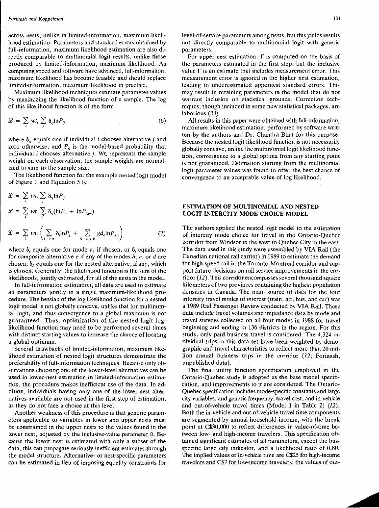
Forinash and Koppelman

across nests, unlike in limited-information, maximum likeli­hood estimation. Parameters and standard errors obtained by full-information, maximum likelihood estimation are also di­rectly comparable to multinomial logit results, unlike those produced by limited-information, maximum likelihood. As computing speed and software have advanced, full-information, maximum likelihood has become feasible and should repface limited-information, maximum likelihood in practice.

Maximum likelihood techniques estimate parameter values by maximizing the likelihood function of a sample. The log of this likelihood function is of the form

:£ = 2: wt; 2: B)nP;j (6) J

where S;j equals one if individual i chooses alternative j and zero otherwise, and P;j is the model-based probability that individual i chooses alternative j. Wt; represents the sample weight on each observation; the sample weights are normal­ized to sum to the sample size.

The likelihood function for the example nested logit model of Figure 1 and Equation 5 is:

:£ = 2: wt; 2: B;jlnP;j i j

:£ = 2: Wt; ( .~ B)nPj + _2: gdklnPkte) 1 1-a,e k-b,c,d

(7)

where Bj equals one for mode a, if chosen, or Bj equals one for composite alternative e if any of the modes b, c, or dare chosen; Bk equals one for the nested alternative, if any, which is chosen. Generally, the likelihood function is the sum of the likelihoods, jointly estimated, for all of the nests in the model.

In full-information estimation, all data are used to estimate all parameters jointly in a single maximum-likelihood pro­cedure. The hessian of the log likelihood function for a nested logit model is not globally concave, unlike that for multinom­ial logit, and thus convergence to a global maximum is not guaranteed. Thus, optimization of the nested-logit log­likelihood function may need to be performed several times with distinct starting values to increase the chance of locating a global optimum.

Several drawbacks of limited-information, maximum like­lihood estimation of nested logit structures demonstrate the preferability of full-information techniques. Because only ob­servations choosing one of the lower-level alternatives can be used in lower-nest estimation in limited-information estima­tion, the procedure makes inefficient use of the data. In ad­dition, individuals having only one of the lower-nest alter­natives available are not used in the first step of estimation, as they do not face a choice at this level.

Another weakness of this procedure is that generic param­eters applicable to variables in lower and upper nests must be constrained in the upper nests to the values found in the lower nest, adjusted by the inclusive-value parameter 0. Be­cause the lower nest is estimated with only a subset of the data, this can propagate seriously inefficient estimates through the model structure. Alternative- or nest-specific parameters can be estimated in lieu of imposing equality constraints for

101

level-of-service parameters among nests, but this yields results not directly comparable to multinomial logit with generic parameters.

For upper-nest estimation, f is computed on the basis of the parameters estimated in the first step, but the inclusive value f is an estimate that includes measurement error. This measurement error is ignored in the higher nest estimation, leading to underestimated uppernest standard errors. This may result in retaining parameters in the model that do not warrant inclusion on statistical grounds. Correction tech­niques, though included in some new statistical packages, are laborious (23).

All results in this paper were obtained with full-information, maximum likelihood estimation, performed by software writ­ten by the authors and Dr. Chandra Bhat for this purpose. Because the nested logit likelihood function is not necessarily globally concave, unlike the multinomial lo git likelihood func­tion, convergence to a global optima from any starting point is not guaranteed. Estimation starting from the multinomial logit parameter values was found to offer the best chance of convergence to an acceptable value of log likelihood.

ESTIMATION OF MULTINOMIAL AND NESTED LOGIT INTERCITY MODE CHOICE MODEL

The authors applied the nested logit model to the estimation of intercity mode choice for travel in the Ontario-Quebec corridor from Windsor in the west to Quebec City in the east. The data used in this study were assembled by VIA Rail (the Canadian national rail carrier) in 1989 to estimate the demand for high-speed rail in the Toronto-Montreal corridor and sup­port future decisions on rail service improvements in the cor­ridor (12). This corridor encompasses several thousand square kilometers of two provinces containing the highest population densities in Canada. The main source of data for the four intercity travel modes of interest (train, air, bus, and car) was a 1989 Rail Passenger Review conducted by VIA Rail. These data include travel volumes and impedance data by mode and travel surveys collected on all four modes in 1988 for travel beginning and ending in 136 districts in the region. For this study, only paid business travel is considered. The 4,324 in­dividual trips in this data set have been weighted by demo­graphic and travel characteristics to reflect more than 20 mil­lion annual business trips in the corridor (12; Forinash, unpublished data).

The final utility function specification employed in the Ontario-Quebec study is adopted as the base model specifi­cation, and improvements to it are considered. The Ontario­Quebec specification includes mode-specific constants and large city variables, and generic frequency, travel cost, and in-vehicle and out-of-vehicle travel times (Model 1 in Table 2) (12). Both the in-vehicle and out-of-vehicle travel time components are segmented by annual household income, with the break point at C$30,000 to reflect differences in value-of-time be­tween low- and high-income travelers. This specification ob­tained significant estimates of all parameters, except the bus­specific large city indicator, and a likelihood ratio of 0.80. The implied values of in-vehicle time are C$25 for high-income travelers and C$7 for low-income travelers; the values of out-

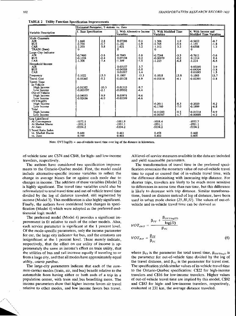
102 TRANSPORTATION RESEARCH RECORD 1413

TABLE 2 Utility Function Specification Improvements

Estimated Parameter, T-statistic vs. Zero

Variable_ Description 1. Base Specification 2. With Alternative Income 3. With Modified Time 4. With Income and Variables Variables Modified Time Variables

Mode Constants AIR 1.888 2.8 0.07286 0.1 1.308 1.9 -0.5652 -0.7 BUS -2.756 -5.7 -1.181 -1.9 -2.705 -5.6 -1.135 -1.8 CAR 2.203 5.8 1.621 3.2 1.312 3.2 0.6588 1.2 TRAIN (Base) 0 0 0 0

Larfie City Indicator AR -0.7460 -3.6 -0.7843 -3.8 -0.7244 -3.5 -0.7611 -3.6 BUS -0.1224 -0.4 0.07158 0.2 -0.06979 -0.2 0.1214 0.4 CAR -1.306 -7.4 -1.309 -7.5 -1.213 -6.8 -1.214 -6.8

Household Income AIR O.o3157 3.7 0.03290 3.9 BUS -0.04308 -3.8 -0.04304 -3.8 CAR 0.01007 1.4 0.01093 1.5

Frequency 0.1022 13.5 0.1007 13.3 0.1018 13.8 0.1005 13.7 Travel Cost -0.03265 -5.2 -0.03128 -4.9 -0.02514 -4.1 -0.02391 -3.8 Travel Time

In-Vehicle High Income -0.01382 -10.3 -0.01315 -9.7 Low Income -0.003797 -2.1 -0.00952 -4.4

Out-of-Vehicle High Income -0.04053 -9.9 -0.03971 -9.6 Low Income -0.02636 -6.0 -0.03399 -6.6

OVT/lo~D) High come -0.2011 -8.3 -0.2020 -8.2 Low Income -0.1760 -7.0 -0.1889 -6.8

Total High Income -0.01283 -9.5 -0.01214 -8.9 Low Income -0.00307 -1.7 -0.00888 -4.2

Log Likelihood At Convergence -1072.1 -1051.9 -1058.4 -1037.7 At Market Shares -1951.1 -1951.1 -1951.1 -1951.1 At Zero -5334.2 -5334.2 -5334.2 -5334.2

L'hood Ratio Index vs. Market Shares 0.448 0.461 0.458 0.468 vs. Zero 0.799 0.803 0.802 0.805

Note: OVT/log(D) = out-of-vehicle travel time over log of the distance in kilometers.

of-vehicle time are C$74 and C$48, for high- and low-income travelers, respectively.

The authors have considered two specification improve­ments to the Ontario-Quebec model. First, the model could include alternative-specific income variables to reflect the change in average biases for or against each mode due to changes in income. The addition of these variables (Model 2) is highly significant. The travel time variables could also be reformulated to total travel time and out-of-vehicle travel time divided by the log of distance traveled, still segmented by income (Model 3). This modification is also highly significant. Finally, the authors have considered both changes in speci­fication (Model 4) which were adopted as the preferred mul­tinomial logit model.

The preferred model (Model 4) provides a significant im­provement in fit relative to each of the other models. Also, each service parameter is significant at the 1 percent level. Of the mode-specific parameters, only the income parameter for car, the large city indicator for bus, and the constants are insignificant at the 1 percent level. These merely indicate, respectively, that the effect on car utility of income is ap­proximately the same as income's effect on train utility, that the utilities of bus and rail increase equally if traveling to or from a large city, and that all modes have approximately equal utility, ceteris paribus.

The large-city parameters indicate that each of the com­mon-carrier modes (train, air, and bus) benefit relative to the automobile from having either or both ends of a trip in a population center, with train and ,bus benefiting more. The income parameters show that higher income favors air travel relative to other modes, and low income favors bus travel.

All level-of-service measures available in the data are included and yield reasonable parameters.

The transformation of travel time in the preferred speci­fication constrains the monetary value of out-of-vehicle travel time to equal or exceed that of in-vehicle travel time, with the difference diminishing with increasing trip distance. For shorter trips, travelers are likely to be much more sensitive to differences in access time than run time, but this difference is likely to decrease with trip distance. Similar transforma­tions, based on distance instead of log of distance, have been used in urban mode choice (25,30,31). The values of out-of­vehicle and in-vehicle travel time can be derived as

'3ovTllog(D) 13rr + log(D)

VOTovT = -----=-''---'--13Tc

VOTwT = ~TT 1-'TC

(8)

where 13rr is the parameter for total travel time, 13ovTttogD is the parameter for out-of-vehicle time divided by the log of the travel distance, and 13Tc is the parameter for travel cost. The specification yields similar values of in-vehicle travel time to the Ontario-Quebec specification: C$22 for high-income travelers and C$16 for low-income travelers. Higher values of out-of-vehicle travel time are implied by this model, C$92 and C$83 for high- and low-income travelers, respectively, evaluated at 231 km, the average distance traveled.

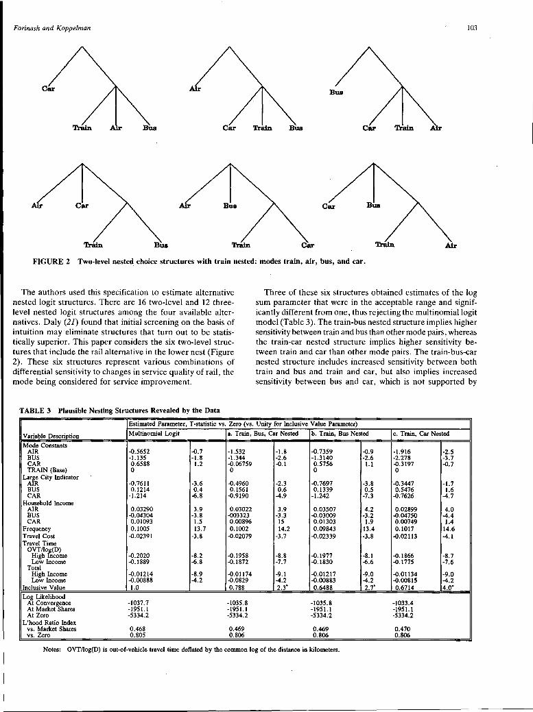
Forinash and Koppelman 103

FIGURE 2 Two-level neste~ choice structures with train nested: modes train, air, bus, and car.

The authors used this specification to estimate alternative nested logit structures. There are 16 two-level and 12 three­level nested logit structures among the four available alter­natives. Daly (21) found that initial screening on the basis of intuition may eliminate structures that turn out to be statis­tically superior. This paper considers the six two-level struc­tures that include the rail alternative in the lower nest (Figure 2). These six structures represent various combinations of differential sensitivity to changes in service quality of rail, the mode being considered for service improvement.

TABLE 3 Plausible Nesting Structures Revealed by the Data

Three of these six structures obtained estimates of the log sum parameter that were in the acceptable range and signif­icantly different from one, thus rejecting the multinomial logit model (Table 3). The train-bus nested structure implies higher sensitivity between train and bus than other mode pairs, whereas the train-car nested structure implies higher sensitivity be­tween train and car than other mode pairs. The train-bus-car nested structure includes increased sensitivity between both train and bus and train and car, but also implies increased sensitivity between bus and car, which is not supported by

Estimated Parameter, T-statistic vs. Zero (vs. Unity for Inclusive Value Parameter) ] Multinomial Logit a. Train, Bus, Car Nested b. Train, Bus Nested c. T - ~· . Variable Description

Mode Constants AIR -0.5652 -0.7 -1.532 -1.8 -0.7359 -0.9 -1.916 -2.5 BUS -1.135 -1.8 -1.344 -2.6 -1.3140 -2.6 -2.278 -3.7 CAR 0.6588 1.2 -0.06759 -0.1 0.5756 1.1 -0.3197 -0.7 TRAIN (Base) 0 0 0 0

Larfie City Indicator AR -0.7611 -3.6 -0.4960 -2.3 -0.7697 -3.8 -0.3447 -1. 7 BUS 0.1214 0.4 0.1561 0.6 0.1339 0.5 0.5476 1.6 CAR -1.214 -6.8 -0.9190 -4.9 -1.242 -7.3 -0.7626 -4.7

Household Income AIR 0.03290 3.9 0.03022 3.9 0.03507 4.2 0.02899 4.0 BUS -0.04304 -3.8 -003323 -3.3 -0.03009 -3.2 -0.04750 -4.4 CAR 0.01093 1.5 0.00896 15 0.01303 1.9 0.00749 1.4

Frequency 0.1005 13.7 0.1002 14.2 0.09843 13.4 0.1017 14.6 Travel Cost -0.02391 -3.8 -0.02079 -3.7 -0.02339 -3.8 -0.02113 -4.1 Travel Time

OVT/log(D) High Income -0.2020 -8.2 -0.1958 -8.8 -0.1977 -8.1 -0.1866 -8.7 Low Income -0.1889 -6.8 -0.1872 -7.7 -0.1830 -6.6 -0.1775 -7.6

Total High Income -0.01214 -8.9 -0.01174 -9.1 -0.01217 -9.0 -0.01134 -9.0 Low Income -0.00888 -4.2 -0.0829 -4.2 -0.00883 -4.2 -0.00815 -4.2

Inclusive Value 1.0 0.788 2.3* 0.6488 2.i 0.6714 4.o·

Log Likelihood At Convergence -1037.7 -1035.8 -1035.8 -1033.4 At Market Shares -1951.l -1951.1 -1951.1 -1951.1 At Zero -5334.2 -5334.2 -5334.2 -5334.2

L'hood Ratio Index vs. Market Shares 0.468 0.469 0.469 0.470 vs. Zero 0.805 0.806 0.806 0.806

Notes: OVT/log(D) is out-of-vehicle travel time deflated by the common log of the distance in kilometers.

104

estimation of a model with bus and car only in the lower nest. Thus, the authors prefer the train-bus and train-car nested structures to the train-bus-car nested structure. The train-car nested structure provides the best fit to the data.

The estimates for the level-of-service parameter estimates for all three structures have the correct sign and are highly significant. Further, these estimates are close to those ob­tained for the multinomial logit model. Thus, the values of time implied by these models are similar to those reported for the multinomial logit model. The parameter estimates for alternative-specific income variables differ somewhat more but are within one standard error in most cases. The param­eter estimates for the alternative-specific constants and large city variables differ considerably among models reflecting the need to adjust these variables to compensate for the changes in model structure.

IMPLICATIONS OF NESTED LOGIT . ESTIMATION FOR PREDICTION OF RAIL SHARES

The demonstration that the nested logit model statistically rejects the multinomial logit model provides important and useful insight into the likely behavioral response of travelers to changes in rail travel service. The authors are also inter­ested in the impact of these changes in model structure on the changes in predicted ridership if specific changes in rail service are undertaken in the future. The authors explored this by estimating the differences in mode choice probabilities predicted for representative individuals traveling between

TABLE 4 Description of Overall and Sample Markets

TRANSPORTATION RESEARCH RECORD 1413

specific city pairs. The ridership predictions were prepared using the incremental logit formulations (32) of the multi­nomial logit model, and the nested logit models with train and bus nested and with train and car nested.

Table 4 presents the market size and current (1987) mode shares for three example markets: Ottawa-Toronto, Toronto­Montreal, and Ottawa-Montreal. Adopting the market shares as representative mode choice probabilities and using average values of all variables, the projected mode probabilities for each city pairs based on the multinomial logit model and the two nested lo git models are reported in Table 5, for a 40 percent reduction in train in-vehicle travel time. This ap­proximates the improvement high-speed rail offers, boosting the line-haul average speed from around 100 km/hr (62 mph) to about 160 km/hr (100 mph). All three models predict a substantial increase in train probability; however, the in­creases for the two nested logit models are substantially higher than for the multinomial logit model (except for the Toronto­Montreal pair for the train-bus nest due to the initial zero mode probability for the bus alternative). The increased rail share results from increased shifting from the other nested alternative, bus or car, to the rail alternative. There is little difference in air shares among the models.

SUMMARY, CONCLUSIONS, AND IMPLICATIONS

This paper demonstrated a statistically significant rejection of the multinomial logit model in favor of three alternative nested

Travel Distance ;) 1987 Train Travel Time 1987 Market Size 1987 Market Shares(%) Market (kilometers t (minutes) (annual business travelers)

Train Air Bus Car

Ottawa- 420 263 459,000 4.87 72.62 1.95 20.56 Toronto

Toronto- 540 295 531,000 8.74 81.00 0.00 10.27 Montreal

Ottawa- 206 121 601,000 9.09 9.27 4.83 76.81 Montreal

TABLE ? Projected Market Shares

Future Market Shares(%) Predicted with 40% Improvement in Train In-Vehicle Travel Time

Train Bus Car Air

Travel .. Market Multinomial :frain/Bus Train/Car MNL TIB TIC MNL T/B TIC MNL T/B TIC NL

Logit Nested Nested NL NL NL NL NL (MNL) Lo git Logit

(TIB NL) (TIC NL)

Ottawa- 14.89 16.32 19.32 1.74 0.98 1.72 18.39 18.25 14.80 64.97 64.45 64.16 Toronto ( +206%) ( +235%) ( +297%) (-11 %) (-50%) (-12%) (-11%) (-11 %) (-28%) (-11 %) (-11%) (-12%)

Toronto- 27.54 27.58 30.61 NR NR NR 8.15 8.15 5.31 64.32 64.27 64.08 Montreal (+2i5%) (+216%) ( +250%) (-21 %) (-21 %) (-48%) (-21 %) (-21%) (-21 %)

Ottawa- 14.96 16.16 17.89 4.52 3.59 4.51 71.85 71.61 68.95 8.67 8.64 8.65 Montreal (+65%) (+78%) (+97%) (-6%) (-26%) (-7%) (-6%) (-7%) (-10%) (-6%) (-7%) (-7%)

Note: NR indicates not relevant, due to zero bus share in base case.

Forinash and Koppelman

logit models. The differences imply substantially greater sen­sitivity of either or both of the car and bus modes to im­provements in rail service. Example predictions of changes in mode probabilities for representative travelers indicate that the adoption of either of the nested logit models would result in substantially higher rail probabilities at the individual level and rail shares at the aggregate level. This result demonstrates the importance of considering alternatives to the multinomial logit structure in intercity mode choice modeling.

Differences between the nested logit models in their be­havior implications and predictions raise serious questions about which of the models to adopt. Different choices result in different rail ridership estimates and different estimates of the mode source of the increased ridership. Despite the sta­tistical rejection of the multinomial logit model and the im­provement in goodness of fit, these results do not provide a satisfactory conclusion to the search for improved specifica­tion of intercity mode choice models. The apparent higher degree of sensitivity both between rail and bus and between rail and car cannot be accommodated in the nested logit struc­ture except by including car and bus in the same nest, a choice that is inconsistent with the empirical analysis. There appears to be a need to consider more sophisticated model structures to adequately represent the subs!itution characteristics among these alternatives.

It is interesting to observe that these estimation results do not support the notion that improved rail service will attract a larger share of travelers from air than from other modes. However, this result is likely to represent only incremental changes in rail service. It seems reasonable to speculate that large improvements in rail service (implementation of high­speed rail or magnetic levitation) may change the competitive structure among intercity travel modes. In this case, the struc­ture of the model may require adjustment to account for the differences in intermodal sensitivity. These results demon­strate a continuing need to develop improved intercity travel demand models.

ACKNOWLEDGMENTS

The primary author was supported during the early part of this research by the Transportation Center at Northwestern University and by a National Science Foundation Graduate Fellowship for a large part of the period. The authors are indebted to the Ontario-Quebec Rapid Train Task Force for allowing the use of the data and to Bruce T. Williams of KPMG Peat Marwick for assembly and documentation of the estimation data file.

REFERENCES

1. Special Report 233: In Pursuit of Speed: New Options for Intercity Passenger Transport. TRB, National Research Council, Wash­ington, D.C., 1991.

2. Terminal Area Forecasts 1987-2000. FAA, U.S. Department of Transportation, 1987.

3. Future Development of the U.S. Airport Network: Preliminary Report and Recommended Study Plan. TRB, National Research Council, Washington, D.C. 1988.

4. Daley Insists Third Airport Dead, Buried. Chicago Tribune, July 2, 1992, Sec. 1, p. l.

105

5. Searles, D. Critics Haven't Grounded Denver Airport. Chicago Tribune, July 19, 1992, Sec. 1, p. 1

6. Moon, F. B. Houston Moves Forward Again. Civil Engineering, VoL 61, No. 2, 1991, pp. 40-43.

7. Hartje, R. L., and G. S. Pfeffer. Private Toll Road: SR 91 Toll Express Lanes. Compendium of Technical Papers. ITE, Wash­ington, D.C., 1991.

8. Dees, D. C., and J. W. Guyton. The Chicago-Kansas City Toll­way Feasibility Study: An Investigation of Private Financing Po­tential. Compendium of Technical Papers. Institute of Trans­portation Engineers, Washington, D.C., 1990.

9. Baer, H., W. Testa, D. Vandenbrink, and B. Williams. High Speed Rail in the Midwest: An Economic Analysis. Federal Re­serve Board of Chicago, Ill., 1984.

10. Detroit-Chicago Corridor High Speed Rail Technical Report. In­tercity Transportation Planning Division, Bureau of Transpor­tation Planning, Michigan Department of Transportation, Lan­sing, 1985.

11. Preliminary Implementation Plan. National Maglev Initiative, U.S. Army Corps of Engineers, June 1990.

12. KPMG Peat Marwick and F. S. Koppelman. Analysis of the Mar­ket Demand for High Speed Rail in the Quebec-Ontario Corridor. Report produced for Ontario/Quebec Rapid Train Task Force. KPMG Peat Marwick, Vienna, Va., 1990.

13. Peat Marwick Main and Co. and F. S. Koppelman. Preparation of Base Year ServiCe Characteristics and Development of Travel Demand Models: Working Paper #3. Report submitted to Ohio High Speed Rail Authority, June 1989.

14. Westin, R. B., and C. F. Manski. Theoretical and Conceptual Developments in Demand Modeling. In Behavioural Travel Mod­eling (D. A. Hensher and P. R. Stopher, eds.), Croom Helm, London, 1979.

15. Hensher, D. A. Efficient Estimation of Hierarchical Logit Mode Choice Models. Proceedings of the Japanese Society of Civil En­gineers, Vol. 425, No. 4, 1991, pp. 17-28.

16. Stephanedes, Y. S., V. Kummer, and B. Padmanabhan. A Fully Disaggregate Mode-Choice Model for Business Intercity Travel. Transportation Planning and Technology, Vol. 9, No. 1, 1984.

17. Stopher, P. R., and J. N. Prashker. Intercity Passenger Fore­casting: The Use of Current Travel Forecasting Procedures. Transportation Research Forum Proceedings: 17th Annual Meet­ing, Vol. XVII, No. 1, 1976, pp. 67-75.

18. Grayson, A. Disaggregate Model of Mode Choice in Intercity Travel. In Transportation Research Record 835, TRB, National Research Council, Washington, D.C., 1981, pp. 36-42.

19. Ellis, R. H., P. R. Rassam, and J. C. Bennett. Consideration of Inter-Modal Competition in the Forecasting of National Intercity Travel. In Highway Research Record 369, HRB, National Re­search Council, Washington, D.C., 1971, pp. 253-261.

20. Ortuzar, J. de D. Nested Logit Models for Mixed-Mode Travel in Urban Corridors. Transportation Research A, Vol. 17, No. 4, 1983, pp. 283-299.

21. Daly, A. Estimating "Tree" Logit Models. Transportation Re­search B, Vol. 21, No. 4, 1987, pp. 251-267.

22. Sobel, K. L Travel Demand Forecasting by Using the Nested Multinomial Logit Model. In Transportation Research Record 775, TRB, National Research Council, Washington, D.C., 1980, pp. 48-55.

23. Brownstone, D., and K. A. Small. Efficient Estimation of Nested Logit Models. Journal of Business and Economic Statistics, Vol. 7, No. 1, 1989, pp. 67-74.

24. Morrison, S. A., and C. Winston. An Econometric Analysis of the Demand for Intercity Passenger Transportation. In Research in Transportation Economics, Vol. 2 (T. E. Keeler, ed.), JAi Press, Inc., Greenwich, Conn., 1983, pp. 213-238.

25. Ben-Akiva, M. E., and S. Lerman. Discrete Choice Analysis: Theory and Application to Travel Demand. Massachusetts Insti­tute of Technology, Cambridge, Mass., 1985.

26. McFadden, D. Conditional Logit Analysis of Qualitative Choice Behavior. In Frontiers in Econometrics (P. Zarembka, ed.), Academic Press, New York, N.Y., 1973.

27. Hensher, D. A. Sequential and Full-Information Maximum -Likelihood Estimation of a Nested Logit Model. The Review of Economics and Statistics, Vol. 68, No. 4, 1986, pp. 657-667.

106

28. Cosslett, S. R. Alternative Estimation of Discrete Choice Models. In Structural Analysis of Discrete Data with Econometric Appli­cations, (C. F. Manski and D. McFadden, eds.), MIT Press, Cam­bridge, Mass., 1981.

29. Forinash, C. V. A Comparison of Model Structures for Intercity Travel Mode Choice. Master's thesis (unpublished). Department of Civil Engineering, Northwestern University, Evanston, Ill., 1992.

30. Koppelman, F. S., and C. G. Wilmot. Transferability Analysis of Disaggregate Choice Models. In Transportation Research Rec­ord 895, TRB, National Research Council, Washington, D.C., 1982.

TRANSPORTATION RESEARCH RECORD 1413

31. Koppelman, F. S., and C. G. Wilmot. The Effect of Omission of Variables on Choice Model Transferability. Transportation Research B, Vol. 20, No. 3, 1986.

32. Koppelman, F. S. Predicting Transit Ridership in Response to Transit Service Changes. Journal of Transportation Engineering, Vol. 109, No. TE4, July 1983.

Publication of this paper sponsored by Committee on Passenger Travel Demand Forecasting.

TRANSPORTATION RESEARCH RECORD 1413 107

Specifying, Estimating, and Validating a New Trip Generation Model: Case Study in Montgomery County, Maryland

AJAY KUMAR AND DAVID LEVINSON

The development of an afternoon peak-period trip-generation model for both work and nonwork trips is discussed. Three data sources are used in model development: a household travel sur­vey, a census update survey, and a trip generation study. Seven one-direction trip purposes are defined, specifically accounting for stops made on the return trip from work to home. Trips are classified by origin and destination activities rather than by pro­duction and attraction, reframing the conventional schema of home-based and non-home-based trips. Before the model was estimated the household travel survey was demographically cal­ibrated against the census update to minimize demographic bias. A model of home-end trip generation is estimated using the household travel survey as a cross-classification of the demo­graphic factors of age and household size in addition to dwelling type. Non-home-end generation uses employment by type and population. The model was validated by comparison with a site­based trip generation study, which revealed an underreporting of the relatively short and less regular shopping trips. Normalization procedures were developed to ensure that all ends of a chained trip were properly accounted for.

This paper discusses the procedures used to specify, estimate, and validate a trip-generation model for both work and non­work trips. The model's temporal focus is on the afternoon peak period (3:30 to 6:30 p.m.) because it is used, among other applications, for. staging development to ensure ade­quate transportation facilities. Studies in Montgomery County, Maryland, have demonstrated that transportation capacity is more of a constraint during the afternoon peak period due to increased non-work travel (1). This paper attempts to com­prehensively account for travel by defining trip sequencing patterns. Modeling chained trips also requires some redefi­nition of conventional normalization procedures, which are described later. By accounting for all modes in trip generation (driver, passenger, transit, walk, and bicycle), it is possible to apply a comprehensive mode choice model that captures the dynamics of changing travel behavior.

The development of an afternoon peak-period travel model has received scant attention in the transportation literature even though temporal clustering of daily trips is a well under­stood phenomenon. In addition, the models constructed by transportation analysts in most metropolitan planning orga­nizations primarily emphasize the journey to work. The ra­tionale for the attention given to the work trip is easy to understand. Although work trips account for only about one­quarter of total household trips, their priority rests on their

Montgomery County Planning Department, 8787 Georgia Avenue, Silver Spring, Md. 20910.

fixed route, their regularity, and their length (work trip dis­tances are longer on average than the distances of nonwork trips). Moreover, the decennial census reports transportation data only on commuter characteristics. However, recent lit­erature brings out the growing importance of nonwork trips and the need to correctly specify nonwork purposes (2).

Ongoing efforts have been made by the Montgomery County Planning Department (MCPD) of the Maryland-National Capital Park and Planning Commission (MNCPPC) to de­velop a transportation planning model, covering metropolitan Washington and Baltimore, that is sensitive to some of the concerns raised against the conventional model applications (3). The most recent version of the MCPD transportation planning model, TRAVEL/2, attempts to account for inter­dependence among trips by looking at specific activities pur­sued at each trip end; this is discussed by Levinson and Kumar in another paper in this Record. The model framework is sensitive to changes in demographic structure and spatial or­ganization. Peak-period trip distribution models are devel­oped consistent with the trip purposes defined in trip gen­eration. A multimodal gravity model formulation is used in trip distribution (4). The model adjusts trave.l demand in re­sponse to changes in transportation network supply and es­timates traffic conditions prevailing during the afternoon peak hour. This paper examines how the trip generation component of the transportation planning model can better include changes in demographics and behavior to improve travel demand estimation.

As the subsequent steps in modeling travel demand are based on estimates derived from the trip-generation stage, the validity of the assumptions in the trip-generation analysis are crucial to the overall quality of the forecasts. After dis­cussing the data used for model estimation, the specific trip purposes used in the study are defined by origin and desti­nation activity. An attempt is made to explicitly account for stops inade on the return trip from work, including a discus­sion of model normalization procedures. Trip-generation fac­tors are estimated for each trip purpose. The model is vali­dated against the site-based person Trip Generation Study.

DATA

Three primary data sources were used in this research. The 1987-1988 Metropolitan Washington Council of Govern­ments (MWCOG) Household Travel Survey was used for model estimation (5). The Montgomery County Planning Depart-

108

ment's 1987 Census-Update Survey allowed the correction for sampling bias in the survey (6). The Montgomery County Trip Generation Study conducted from 1986 to 1988 provided a means to validate the model against site-based trip generation rates (7).

MWCOG Household Travel Survey

The data on demographics and travel behavior were obtained from the 1987-88 Household Travel Survey. This was the first major regional travel survey conducted in the Washington area since 1968. More than 20,000 randomly selected house­holds in the regions were contacted by telephone and asked to record all trips made by members of their household for a preselected weekday. Approximately 8,000 of these house­holds, making 55,000 trips, completed and returned by mail the travel diaries sent to them. Up to three follow-up calls were made to each household to obtain completed travel diaries.

The data collection for this survey was conducted in two segments. The first segment was conducted from March to July 1987, and the second segment was conducted from March to July 1988. The initial survey design was to collect 2,000 samples each for the District of Columbia, Maryland, and Virginia. Montgomery County and the city of Alexandria con­tracted with MWCOG to collect additional samples in their jurisdictions, resulting in just under 1 percent of Montgomery County residents being sampled. In 1988, the Maryland coun­ties of Charles and Frederick were added to the survey and an additional 500 samples were collected for each of these jurisdictions. The number of completed samples from each of the jurisdictions is given in Table 1.

Household data from the MWCOG Round IV Cooperative Forecasts were used to expand the survey results to regional control totals. The survey data were adjusted to match re­gional household size and vehicle ownership characteristics using marginal weighting techniques. Because these survey data were a nonrepresentative sample, they were corrected for sampling bias.

Montgomery County Census-Update Survey

The Montgomery County Planning Department collects dem­ographic and some basic travel data for Montgomery County

TABLE 1 Sample Size by Jurisdiction

Jurisdiction

Washington. OC Montgomery County. MD Prince George's County, MD Arlington COl.Ulty, VA Alexandria Gty, VA Fairfax County, VA Loudoun County, VA Prince William County, VA Frederick County, MD

Tola!

No. of Completed Samples

1,952 1,827

992 2UJ 378

1,059 258 288 481

7,501

Household Sample Size Size

(in '000) (%)

250 0.78 28) 0.65 263 0.38 48 0.55 79 0.48

328 0.32 31 0.83 89 0.32

1,368 0.55

TRANSPORTATION RESEARCH RECORD 1413

every 4 years to supplement the decennial census data. The 1987 census update is based on a 5 percent sample and was conducted during April 1987. This survey updated informa­tion previously reported in the 1980 U.S. Census, providing information more specific to current planning issues in Mont­gomery County. About 22,000 survey forms were mailed to a carefully designed random sample of county households, and nearly 63 percent of the 13,900 recipients voluntarily sent back valid responses. Collected data were adjusted on the basis of known household and school enrollment distributions to provide reliable county information.

Montgomery County Trip Generation Study

Douglas & Douglas, Inc., assisted by Gorove/Slade Associ­ates, Inc., and Dynamic Concepts for data collection, per­formed a comprehensive study of person and vehicle trip gen­eration for several important land-use types for sites in Montgomery County, Maryland. The number of trips made to and from a total of 162 sites were surveyed, including 79 commercial office buildings, 59 residential sites, 15 shopping centers, and 9 fast food restaurants. Vehicle occupancy and walk in and out were separately observed from vehicle trips to obtain person trip rates. The study has produced a trip­generation data set based on a statistically reliable and ran­domly selected collection of development sites.

CORRECTING FOR BIAS IN HOUSEHOLD TRAVEL SURVEY

The key data base used to estimate trip-generation coefficients and rates was the 1987-88 Household Travel Survey. How­ever, as observed earlier, this survey, although rich in de­scribing travel behavior, was based on a less than 1 percent sample in Montgomery County. Because the county also con­ducts a survey to update the census that is based on a 5 percent sample, it was possible to calibrate the household travel survey to the larger sample. The hypothesis of this exercise is that the household travel survey does not truly represent all seg­ments of the population. Thus, there is a need to compensate for the underrepresentation of particular groups to properly replicate the observed population distribution as a prereq­uisite to estimating true travel behavior from the survey. This section focuses on the differences among some of the demo­graphic variables between the two surveys and the rationale for calibrating the household travel survey. A detailed meth­odology on calibrating the two sets is provided by Kumar (8).

To examine the differences between the two sets, a cross­tabulation (Table 2) was prepared displaying the number of dwelling types (single family, townhouses, apartments), by the number of persons in the households (1, 2, 3, and 4 plus), by the gender of the household head, for both the MWCOG household travel survey and the MCPD census update sam­ples. Though the definition of household head can never be specific, it is important to identify single-parent females who are heads of households, because they represent a growing proportion of the population and often occupy lower ranks in the household income distribution. Underrepresentation of households with a female head carries the implication of underrepresenting low-income households.

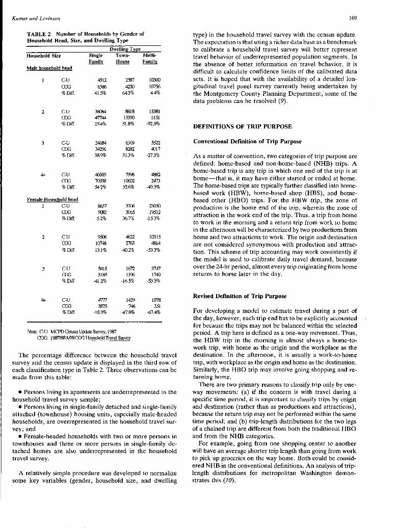
Kumar and Levinson

TABLE 2 Number of Households by Gender of Household Head, Size, and Dwelling Type

Dwelling Tl'.Ee Household Size Sln2le Town- Multi-

Family House Family Male household head

C-U 4512 2$7 lCBOO ax; 6386 4250 10756 %Diff. 41.5% 643% 4.4%

2 C-U 3~ 8818 15381 ax; 47744 133~ 1151 %Diff. 25.4% 51.8% -92.5%

3 C-l.i 24684 63(1) 5522 ax; 34296 8282 4017 %DilT. 38.9% 31.3% -27.3%

4t C-U 4(i(XJ) 7Wi!, 4882 ax; 7(1).38 1ocm 2473 %Diff. 54.2% 32.6% -49.3%

Female Household head 1 C-U '8£37 37CX> ~

ax; ~ ~ 19512 %DilT. 5.2% 36.7% -15.3%

2 C-U 9.:n:i 4622 lffi15 ax; 10748 27@ 4814 %Diff. 13.1% -40.2% -53.3%

3 C-U 5415 1672 3747 ax; 318.5 1396 1749 %Diff. -41.2% -16.5% -53.3%

C-U 4m 1429 1078 ax; 3875 746 351 %DilT. -18.9% -47.8% -67.4%

Note: C-U: MCPD Census Update Smvey, 1987 COO: 1 ~/88 MWCOO Ho!!§eho!d T@Y_~_ Survey

The percentage difference between the household travel survey and the census update is displayed in the third row of each classification type in Table 2. Three observations can be made from this table:

• Persons living in apartments are underrepresented in the household travel survey sample;

•Persons living in single-family detached and single-family attached (townhouse) housing units, especially male-headed households, are overrepresented in the household travel sur­vey; and

•Female-headed households with two or more persons in townhouses and three or more persons in single-family de­tached homes are also underrepresented in the household travel survey.

A relatively simple procedure was developed to normalize some key variables (gender, household size, and dwelling

109

type) in the household travel survey with the census update. The expectation is that using a richer data base as a benchmark to calibrate a household travel survey will better represent travel behavior of underrepresented population segments. In the absence of better information on travel behavior, it is difficult to calculate confidence limits of the calibrated data sets. It is hoped that with the availability of a detailed lon­gitudinal travel panel survey currently being undertaken by the Montgomery County Planning Department,· some of the data problems can be resolved (9).

DEFINITIONS OF TRIP PURPOSE

Conventional Definition of Trip Purpose

As a matter of convention, two categories of trip purpose are defined: home-based and non-home-based (NHB) trips. A home-based trip is any trip in which one end of the trip is at home-that is, it may have either started or ended at home. The home-based trips are typically further classified into home­based work (HBW), home-based shop (HBS), and home­based other (HBO) trips. For the HBW trip, the zone of production is the home end of the trip, whereas the zone of attraction is the work end of the trip. Thus, a trip from home to work in the morning and a return trip from work to home in the afternoon will be characterized by two productions from home and two attractions to work. The origin and destination are not considered synonymous with production and attrac­tion. This scheme of trip accounting may work consistently if the model is used to calibrate daily travel demand, because over the 24-hr period, almost every trip originating from home returns to home later in the day.

Revised Definition of Trip Purpose

For developing a model to estimate travel during a part of the day, however, each trip end has to be explicitly accounted for because the trips may not be balanced within the selected period. A trip here is defined as a one-way movement. Thus, the HBW trip in the morning is almost always a home-to­work trip, with home as the origin and the workplace as the destination. In the afternoon, it is usually a work-to-home trip, with workplace as the origin and home as the destination. Similarly, the HBO trip may involve going shopping and re­turning home.

There are two primary reasons to classify trip only by one­way movements: (a) if the concern is with travel during a specific time period, it is important to classify trips by origin and destination (rather than as productions and attractions), because the return trip may not be performed within the same time period; and (b) trip-length distributions for the two legs of a chained trip are different from both the traditional HBO and from the NHB categories.

For example, going from one shopping center to another will have an average shorter trip length than going from work to pick up groceries on the way home. Both could be consid­ered NHB in the conventional definitions. An analysis of trip­length distributions for metropolitan Washington demon­strates this (JO).

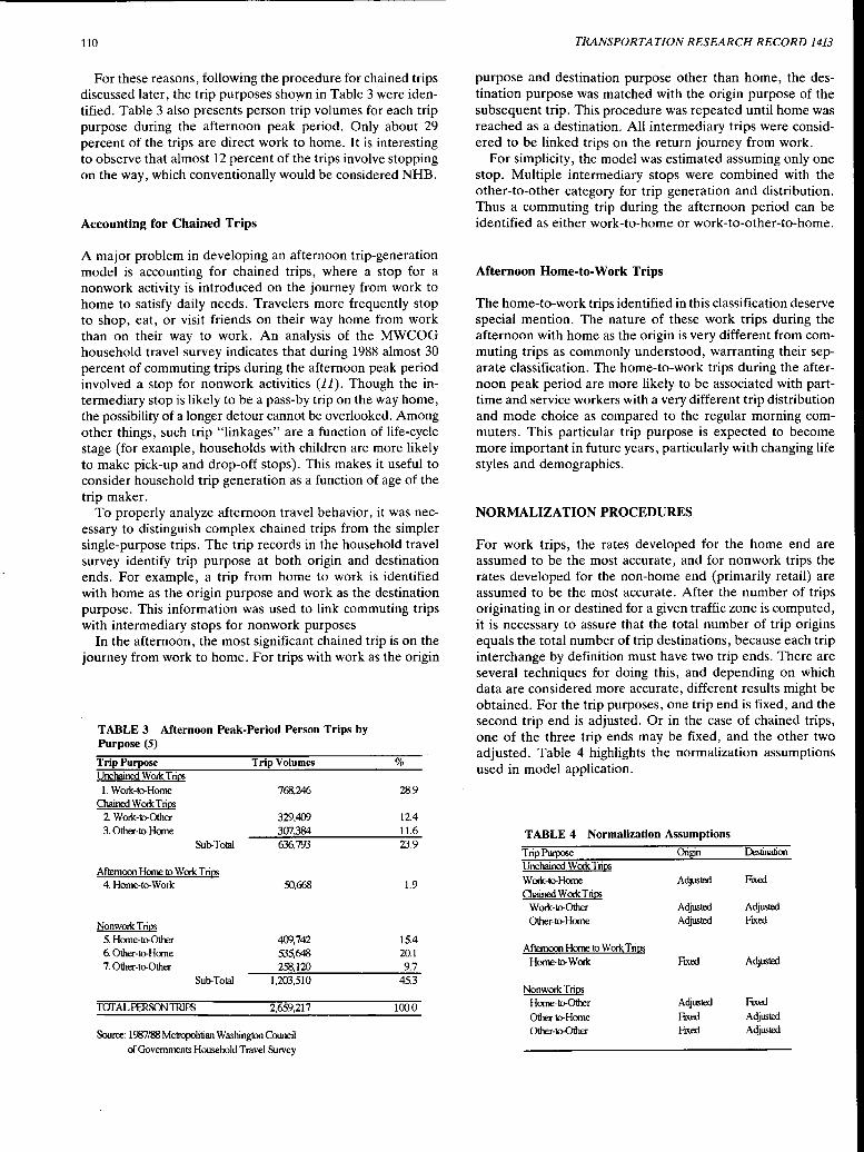
110

For these reasons, following the procedure for chained trips discussed later, the trip purposes shown in Table 3 were iden­tified. Table 3 also presents person trip volumes for each trip purpose during the afternoon peak period. Only about 29 percent of the trips are direct work to home. It is interesting to observe that almost 12 percent of the trips involve stopping on the way, which conventionally would be considered NHB.

Accounting for Chained Trips

A major problem in developing an afternoon trip-generation model is accounting for chained trips, where a stop for a nonwork activity is introduced on the journey from work to home to satisfy daily needs. Travelers more frequently stop to shop, eat, or visit friends on their way home from work than on their way to work. An analysis of the MWCOG household travel survey indicates that during 1988 almost 30 percent of commuting trips during the afternoon peak period involved a stop for nonwork activities (11). Though the in­termediary stop is likely to be a pass-by trip on the way home, the possibility of a longer detour cannot be overlooked. Among other things, such trip "linkages" are a function of life-cycle stage (for example, households with children are more likely to make pick-up and drop-off stops). This makes it useful to consider household trip generation as a function of age of the trip maker.

To properly analyze afternoon travel behavior, it was nec­essary to distinguish complex chained trips from the simpler single-purpose trips. The trip records in the household travel survey identify trip purpose at both origin and destination ends. For example, a trip from home to work is identified with home as the origin purpose and work as the destination purpose. This information was used to link commuting trips with intermediary stops for nonwork purposes

In the afternoon, the most significant chained trip is on the journey from work to home. For trips with work as the origin

TABLE 3 Afternoon Peak-Period Person Trips by Purpose (5)

Trip Purpose Trip Volumes Unchained Work Tri~

1. Work-to-Home 768,246 Olained Work Tri~

2 Work-to-Other 329,4()1) 3. Other-to-Home 307,384

Sub-Total 6.36,793

Afternoon Home to Work Tri~ 4. Home-to-Work 50,668

Nonwork Trios 5. Home-to-Other 400,742 6. Other-to-Home 535,648 7. Other-to-Other 258,120

Sub-Total 1,203,510

TOf ALPERSON1RIPS 2,659,217

Source: l~/88 Metropolitian Washington Council of Governments Household Travel Survey

%

28.9

12.4 11.6 23.9

1.9

15.4 20.l 9.7

45.3

100.0

TRANSPORTATION RESEARCH RECORD 1413

purpose and destination purpose other than home, the des­tination purpose was matched with the origin purpose of the subsequent trip. This procedure was repeated until home was reached as a destination. All intermediary trips were consid­ered to be linked trips on the return journey from work.

For simplicity, the model was estimated assuming only one stop. Multiple intermediary stops were combined with the other-to-other category for trip generation and distribution. Thus a commuting trip during the afternoon period can be identified as either work-to-home or work-to-other-to-home.

Afternoon Home-to-Work Trips

The home-to-work trips identified in this classification deserve special mention. The nature of these work trips during the afternoon with home as the origin is very different from com­muting trips as commonly understood, warranting their sep­arate classification. The home-to-work trips during the after­noon peak period are more likely to be associated with part­time and service workers with a very different trip distribution and mode choice as compared to the regular morning com­muters. This particular trip purpose is expected to become more important in future years, particularly with changing life styles and demographics.

NORMALIZATION PROCEDURES

For work trips, the rates developed for the home end are assumed to be the most accurate, and for nonwork trips the rates developed for the non-home end (primarily retail) are assumed to be the most accurate. After the number of trips originating in or destined for a given traffic zone is computed, it is necessary to assure that the total number of trip origins equals the total number of trip destinations, because each trip interchange by definition must have two trip ends. There are several techniques for doing this, and depending on which data are considered more accurate, different results might be obtained. For the trip purposes, one trip end is fixed, and the second trip end is adjusted. Or in the case of chained trips, one of the three trip ends may be fixed, and the other two adjusted. Table 4 highlights the normalization assumptions used in model application.

TABLE 4 Normalization Assumptions

Trip Purpose Origin Destination Unchained Work Tri~ Work-to-Home Adjusted Fixed Olained Work Tri~

Work-to-Other Adjusted Adjusted Other-to-Home Adjusted Fixed

Afternoon Home to Work Tri~ Home-to-Work Fixed Adjusted

NonworkTrios Home-to-Other Adjusted FIX.ed

Other-to-Home FIX.ed Adjusted Other-to-Other FIX.ed Adjusted

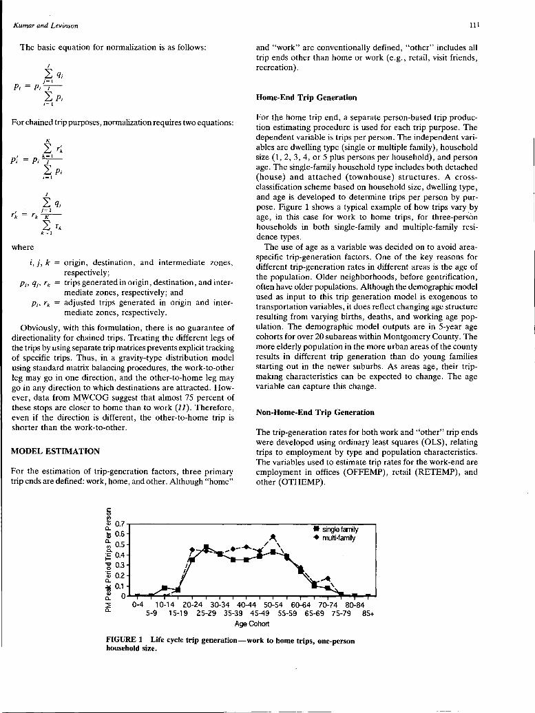
Kumar and Levinson

The basic equation for normalization is as follows:

J

2:% j=l Pi= Pi_1 __

LPi i=l

For chained trip purposes, normalization requires two equations:

where

i, j, k = ongm, destination, and intermediate zones, respectively;

pi, qj, rk = trips generated in origin, destination, and inter­mediate zones, respectively; and

pi, rk = adjusted trips generated in origin and inter­mediate zones, respectively.

Obviously, with this formulation, there is no guarantee of directionality for chained trips. Treating the different legs of the trips by using separate trip matrices prevents explicit tracking of specific trips. Thus, in a gravity-type distribution model using standard matrix balancing procedures, the work-to-other leg may go in one direction, and the other-to-home leg may go in any direction to which destinations are attracted. How­ever, data from MW COG suggest that almost 75 percent of these stops are closer to home than to work (11). Therefore, even if the direction is different, the other-to-home trip is shorter than the work-to-other.

MODEL ESTIMATION

For the estimation of trip-generation factors, three primary trip ends are defined: work, home, and other. Although "home"

111

and "work" are conventionally defined, "other" includes all trip ends other than home or work (e.g., retail, visit friends, recreation).

Home-End Trip Generation

For the home trip end, a separate person-based trip produc­tion estimating procedure is used for each trip purpose. The dependent variable is trips per person. The independent vari­ables are dwelling type (single or multiple family), household size (1, 2, 3, 4, or 5 plus persons per household), and person age. The single-family household type includes both detached (house) and attached (townhouse) structures. A cross­classification scheme based on household size, dwelling type, and age is developed to determine trips per person by pur­pose. Figure 1 shows a typical example of how trips vary by age, in this case for work to home trips, for three-person households in both single-family and multiple-family resi­dence types.

The use of age as a variable was decided on to avoid area­specific trip-generation factors. One of the key reasons for different trip-generation rates in different areas is the age of the population. Older neighborhoods, before gentrification, often have older populations. Although the demographic model used as input to this trip generation model is exogenous to transportation variables, it does reflect changing age structure resulting from varying births, deaths, and working age pop­ulation. The demographic model outputs are in 5-year age cohorts for over 20 subareas within Montgomery County. The more elderly population in the more urban areas of the county results in different trip generation than do young families starting out in the newer suburbs. As areas age, their trip­making characteristics can be expected to change. The age variable can capture this change.

Non-Home-End Trip Generation

The trip-generation rates for both work and "other" trip ends were developed using ordinary least squares (OLS), relating trips to employment by type and population characteristics. The variables used to estimate trip rates for the work-end are employment in offices (OFFEMP), retail (RETEMP), and other ( OTHEMP).

0-4 10-14 20-24 30-34 40-44 50-54 60-64 70-74 80-84 5-9 15-19 25-29 35-39 45-49 55-59 65-69 75-79 85+

A<JS Cohort

FIGURE 1 Life cycle trip generation-work to home trips, one-person household size.

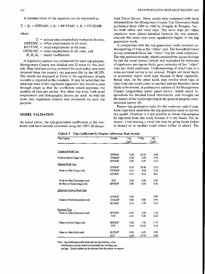
112

A standard form of the equation can be expressed as:

T; = B1 x OFFEMP; + B2 x RETEMP; + B 3 x OTHEMP;

where

T; = person trips attracted per worker in ith zone, OFFEMP; office employment in ith zone, RETEMP; = retail employment in ith zone, OTHEMP; = other employment in ith zone, and

B1 ,B2 ,B3 = model coefficients.

A regression analysis was conducted for each trip purpose. Montgomery County was divided into 22 areas for this anal­ysis. Base land-use activity numbers for each policy area were obtained from the county's tax assessors file by the MCPD. The results are displayed in Table 5; the significance of each variable is reported in the t-statistic. It may be noted that the intercept term of the regression equations was forced to pass through origin so that the coefficient would represent the number of trips per person. For other trip ends, both retail employment and demographic factors are used. As with the work end, regression analysis was conducted for each trip purpose.

MODEL VALIDATION

As noted above, the trip-generation coefficients at the non­home end were initially estimated using the 1987-88 House-

TRANSPORTATION RESEARCH RECORD 1413

hold Travel Survey. These results were compared with those obtained from the Montgomery County Trip Generation Study performed from 1986 to 1988 by Douglas & Douglas, Inc., for both office and retail trips. The work trips per office employee were almost identical between the two sources, whereas the retail rates were significantly higher in the trip generation study.

A comparison with the trip generation study revealed un­derreporting of trips at the "other" end. The household travel survey estimated about one "other" trip per retail employee. The trip generation study, which contained the square footage by site for retail centers (which was multiplied by estimates of employees per square foot), gave estimates of five "other" trips per retail employee. Underreporting of retail trips in a cross-sectional survey is not unusual. People are more likely to accurately report work trips because of their regularity. Retail trips, on the other hand, may involve short trips or trips from one retail center to another and are therefore more likely to be missed. A preliminary analysis of the Montgomery County longitudinal travel panel survey, which asked re­spondents for detailed travel information, also brought out the nature of the underreporting in the general-purpose cross­sectional survey ( 8).

Person trip generation rates for the nonhome end of non­work trips were used from the trip generation study to correct the model. However it is not possible to obtain trip-purpose by trip-ends from this study because it is site based. For in­stance, a trip leaving a retail site may be going home (other to home) or to another retail center (other to other). The

TABLE 5 Trip Coefficients by Purpose (Afternoon Peak Period)

Trip Purpose Vari~e Trip T-Stat Adj. Coe ff. Coe ff.

Unchained Work Tri~ OFFFMP 0.50 22.42 0.50

Work-to-Home (Origin end) 011-IHv1P 0.36 3.95 0.35 REIBv1P 0.()C) 0.47 0.10

Oiained Work Tri~ OFFFMP 0.19 20.08 0.19

Work-to-Other (Origin end) 011-IHv1P 0.16 4.02 0.16

REIBv1P 0.01 0.14 0.01

Worlc-to-Other (Destination end) K>P 0.03 3.20 0.03 & Other-to-Home (Origin end) REIBv1P 0.56 6.04 0.56

Afternoon Home to Work Tri~

OFFFMP 0.00 0.00 Home-to-Work(IX:stination end) 011-IHv1P 0.01 0.80 0.01

REIBv1P 0.14 1.99 0.14

Nonwork Trips Home-to-Other (IX:stination end) REIBv1P 0.22 1.83 1.10

K>P 0.10 7.49 0.10

Other-to-Home (Origin end) REIBv1P 0.22 1.93 1.10 K>P 0.14 10.52 0.14

Other-to-Other (Both ends) REIBv1P 0.20 4.41 3.20

FOP 0.05 10.75 0.05

Note: Trip coefficients at the home end are calculated by a cross-classification scheme based on household size, dwelling type, and age Detailed tables can be obtained from the authors on request

Kumar and Levinson

distribution among different trip purposes was assumed sim­ilar to that obtained from the household travel survey. Table 5 shows the RETEMP coefficients from the household travel survey before and after adjustment using the trip generation study.

CONCLUSIONS

This paper covers two important applications: (a) integrating several survey data sets and using a benchmark data set to validate model results and (b) specifying an afternoon peak­period trip-end trip-generation model in an attempt to better replicate travel demand and capture the intermediate stops that characterize many of the trips from work to home. Re­lated research indicates that chained work trips are a signif­icant component of afternoon travel. Simplifying these trips, or misclassifying them, would clearly lead to an misreporting of total travel. Classification of chained work trips, such as work-to-shop-to-home as nonwork trips or non-home-based trips will result in a misspecification of the model.

The person-based afternoon peak-period trip-generation model estimated uses three factors-age, household size, and dwelling type-to determine trip generation. Other factors affecting trip-making behavior for both work and nonwork trips, such as income and accessibility, will be used in further refinements of the model as better data become available. Efforts are under way in Montgomery County to collect these data as part of the ongoing longitudinal travel panel survey. Changing behavior over time, such as the increase in female labor force participation, has also altered trip generation. Any future attempt to validate this model's output against histor­ical data needs to account for this changing behavior.

Transportation planning models are becoming increasingly important because of the Clean Air Act Amendments of 1990 and the Intermodal Surface Transportation Efficiency Act of 1991. Major decisions are being affected by the outputs of transportation planning models. Trip generation, as the first stage in travel demand estimation, is extremely important in the final outcome of model results.

ACKNOWLEDGMENTS

This research was funded by the MCPD. Robert Winick, Michael Replogle, the staff of the MCPD, the MCPD Trans-

113

portation Modeling Technical Advisory Committee, and the MWCOG/Transportation Planning Board Travel Forecasting Subcommittee provided useful comments. The advice and -recommendations of Gang Len Chang, Everett Carter, and Paul Schonfeld of the University of Maryland on part of this work should also be noted. The helpful comments of three anonymous referees are appreciated.

REFERENCES

1. Levinson, D., and A. Kumar. Operational Evidence for Changing Travel Patterns. Working paper. Montgomery County Planning Department, Silver Spring, Md. 1992.

2. Gordon, P., A. Kumar, and H. W. Richardson, Beyond the Journey to Work. Transportation Research A, Vol. 22A, No. 6, 1988, pp. 419-426.

3. Replogle, M. Computer Transportation Models for Land Use Regulation and Master Planning in Montgomery County, Mary­land. In Transportation Research Record 1262, TRB, National Research Council, Washington, D.C., 1990, pp. 91-100.

4. Levinson, D., and A. Kumar. Development of a Multi-modal Trip Distribution Model. Working paper. Montgomery County Planning Department, Silver Spring, Md. 1992.

5. 1987-88 Household Travel Survey. Metropolitan Washington Council of Governments, Washington, D.C., 1988.

6. 1987 Census-Update Survey. Montgomery County Planning De­partment, Silver Spring, Md., 1987.

7. Douglas & Douglas, Inc. Montgomery County Trip Generation Study. Montgomery County Planning Department, Silver Spring, Md., 1989:

8. Kumar, A. Assessing and Correcting for Sampling Bias in a Household Travel Survey. Working paper. Montgomery County Planning Department, Silver Spring, Md., 1990.

9. Kumar, A., and M. Replogle. Low-Cost Trip Purpose Panel Survey: A Case Study of Montgomery County, Maryland. Pre­sented at the 1st U.S. Conference on Panels for Transportation Planning, Lake Arrowhead, Calif., Oct. 1992.

10. Levinson, D., and A. Kumar. The Rational Locator. Why Travel Times Have Remained Stable. Working paper. Montgomery County Planning Department, Silver Spring, Md., 1992.

11. Kumar, A., and D. Levinson. Understanding Chained Trips: Who, When, Where, and How. Working paper. Montgomery County Planning Department, Silver Spring, Md., 1992.

Publication of this paper sponsored by Committee on Passenger Travel Demand Forecasting.

114 TRANSPORTATION RESEARCH RECORD 1413

Equilibrium Assignment Method for Pointwise Flow-Delay Relationships

A. REGUEROS, J. PRASHKER, AND D. MAHALEL

Most _equilibrium traffic assignment models are based on aggre­gate lmk performance functions. These flow-delay functions rep­resent a crude abstraction of real dependence of travel time on a_ctual traffic volumes and physical conditions of the transporta­tion network elements. To achieve more realistic assignment re­sults for planning purposes and in the field of intelligent vehicle­highway systems research, several recent works attempt to com­bin_e assignment with network simulation. A new equilibrium ass_ignn:ient model that can obtain travel time values from any pomtw1se volume-delay function is presented. The proposed so­lution procedure is based on the convex combination method. The proposed assignment procedure is compared with the classic Lebl~nc's assign~ent algorithm with fully specified volume-delay functions and with the method of successive averages used in stochastic assignment problems. The proposed method was found to be superior to the MSA procedure due to its faster and more accurate convergence characteristics.

Many transportation planners and researchers have recently faced the need to solve user equilibrium or system optimum network assignment problems without the use of explicitly defined flow-delay functions. Efficient solution methods that exist to handle these assignment problems cannot be used when the flow-delay functions are not explicitly specified as continuous mathematical functions. Typically flow-delay functions such as that developed by the Bureau of Public Roads (BPR) (J) and other more sophisticated functions rep­resent crude abstraction of links, intersections, and other net­work element characteristics. These performance functions reflect the travel impedance associated with the various net­work elements. The use of these crude aggregate flow-delay functions can easily be justified in long- and medium-range transportation studies where the details of the network's ele­ments cannot be expressed with great accuracy. However, in many recent applications, these aggregate flow-delay func­tions cannot be used.

When traffic assignment is applied to short-range detailed network planning or as a decision support tool for traffic control strategies, the characteristics of the network elements must be presented with great accuracy. Often simulation models are used to achieve the desired degree of realistic represen­tation of the network element characteristics. The output of the simulation models must be incorporated into an efficient traffic assignment procedure to produce traditional traffic as­signment results.

In the field of intelligent vehicle-highway systems (IVHS) research, several recent investigations have identified the im-

Department of Civil Engineering and Transportation Research In-stitute TECHNION, Israel. .

pact of various real-time navigation and control strategies on driver behavior and network congestion. Driver behavior in the controlled network environment is usually represented by elaborate simulation models. Based on behavioral assump­tions, these models predict how a single driver or a small group of drivers will react to traffic conditions and available route guidance information. The movement of each individual driver is governed by a behavioral simulation model. How­ever, to predict the impact of the proposed control strategies on network flows, the results of the simulation stage must be combined by a mathematical process to achieve internally consistent traffic assignment results. Consistent results, in this context, mean that a priori assumptions of the simulation model, for example, regarding travel time considerations, are not violated due to congestion effects.

At present the simulation results are incorporated into user equilibrium or system optimum assignment procedures in one of two methods. In transportation planning applications, a heuristic method of successive iterations that alternates be­tween a flow-delay curve fitting step and a traditional assign­ment step is usually performed. A typical example of this approach is used by the Simulation and Assignment of Traffic to Urban Road Networks software package (SATURN) (2). This software will be discussed further later. In other appli­cations, especially in IVHS research, a method of successive averages (MSA) first suggested by Sheffi (3) is frequently used. The two solution methods mentioned above are not completely satisfactory. A more efficient assignment method that can incorporate simulation results into an assignment procedure is still needed.

In the framework of this work, a traffic assignment model is developed that can use flow-delay functions whose explicit mathematical formulation is unknown. This paper proposes a method that can be applied to solve network flow problems. Based on empirical investigation, this solution will be valid as long as the flow-delay curves are nondecreasing when traffic flow increases. The flow-delay function can be a numeric pointwise function or a set of simulation-generated values. Although the proposed solution procedure is stated as a heu­ristic procedure (the proof of this method is being developed) the presentation follows the Frank-Wolfe method as applied by Leblanc ( 4) to solve for user equilibrium in networks.

ASSIGNMENT AND FLOW-DELAY FUNCTIONS

In traditional transportation planning applications, all the sup­ply characteristics of a given network topology are supposed to be captured by the flow-delay functions. When a complex

Regueros et al.

phenomenon like traffic flow is represented by a relatively simple function with a very limited number of explanatory variables, this representation must be crude and aggregate. Therefore, existing flow-del_ay functions can only coarsely ap­proximate real traffic flow relationships. Yet, due to math­ematical convenience and computer efficiency, those primi­tive flow-delay functions are widely used.

When flow-delay functions are used in an- assignment pro­cedure, they must possess some mathematical properties to achieve unique convergence of the assignment procedures. To achieve unique solution of user equilibrium or system optimum assignment under steady-state deterministic con­ditions, volume-delay curves must satisfy the following properties:

• The functions should be monotone and nondecreasing. • The functions should be continuous and differentiable. •The functions should be defined for all positive values.

This means that the function must exist in the region where volume exceeds capacity.

The last property is necessa_ry because in typical assignment applications, inherently nonsteady-state problems are solved as if steady-state conditions prevail. Thus, temporal delays on network elements that experience demand higher than capacity are implicitly accounted for by the oversaturated region of volume-delay functions.

Many flow-delay functions have been developed for use in traffic assignment problems. Most of these functions define the characteristics of links or approaches to signalized inter­sections. Ortuzar (5) reviewed some of these flow-delay curves. Link functions were developed by the early Detroit trans­portation study and by Davidson (6). The function that is most commonly used was developed by BPR (1) and is defined as follows:

where

t = travel time, t0 = free-flow travel time, X = flow, C = link's capacity, and

ex and 13 = calibration parameters.

(1)

The most commonly used functions to evaluate flow-delay . characteristics on signalized intersection approaches are the classic Webster delay function (7) and ·a function developed by Akcelik (8). Davidson's link model and Webster's inter­section model are not defined when flow exceeds capacity. Travel-time functions of these two models are asymptotic functions, approaching infinite travel times when flow ap­proaches capacity.

Many transportation applications require more realistic as­signment results than can be obtained with the existing flow­delay functions. Delay models must be improved and ex­panded to handle network elements, such as nonsignalized intersections and weaving and merging sections on freeways.

115

To overcome the limitations of coarse and aggregate delay functions, some assignment models use network simulation procedures to evaluate delays. At present, a common char­acteristic of these assignment-simulation models is an iterative loop between a curve-fitting phase of flow-delay functions based on results generated by the simulation run and a tra­ditional assignment phase. The curve-fitting phase is quite complex, requiring substantial computer time, memory, and storage space to generate the estimated flow-delay curves. A set of flow-delay functions generated in one simulation phase are used in a traffic assignment procedure carried to conver­gence. Based on the assignment results, successive iterations of the curve-fitting procedure are performed until the process converges (it is hoped). The problem with this process is that typically no a priori information exists about the real shape of the flow-delay curves, and there is no assurance that the chosen function used in the curve-fitting phase actually rep­resents the real network element behavior. Futhermore, there is no assurance that the chosen functional form will lead the assignment procedure to converge to the correct solution. Two well-documented applications of this process are SA TURN (9) primarily developed to handle transportation planning problems and a model developed by Stephanedes et al. (10) to assist in traffic control issues.

This paper presents a new assignment methodology to in­tegrate simulation with conventional equilibrium assignment. The suggested approach efficiently uses memory and storage resources, but it does not assume a functional form of the flow-delay relations. This inethod iterates between simulation and assignment steps until the assignment procedure converges.

EXACT PROBLEM FORMULATION

To achieve a complete presentation of the proposed method, the process begins with a concise derivation of the steady­state user equilibrium traffic assignment problem following Leblanc's ( 4) work. Next, the MSA suggested by Sheffi (3) to solve stochastic assignment problems is presented. Finally, the new linearization method (LAM) is presented and com­pared with the MSA method. The comparison is based on the results of the two methods relative to the solution of an exact Leblanc's algorithm.

Current Equilibrium Assignment Practice

Beckman et al. (11) formulated the user equilibrium (UE) problem as a convex (nonlinear) objective function under a set of linear constraints. Leblanc ( 4) proposed an efficient algorithm to solve this problem, when flow-delay functions are fully specified, based on the Frank-Wolfe method (12). The steady-state UE problem is formulated as follows:

min f(x) = 2-: J: t(w)dw I]

(2)

st: D(j, s) + 2: xfi = 2: xjk j k

vi, s (3)

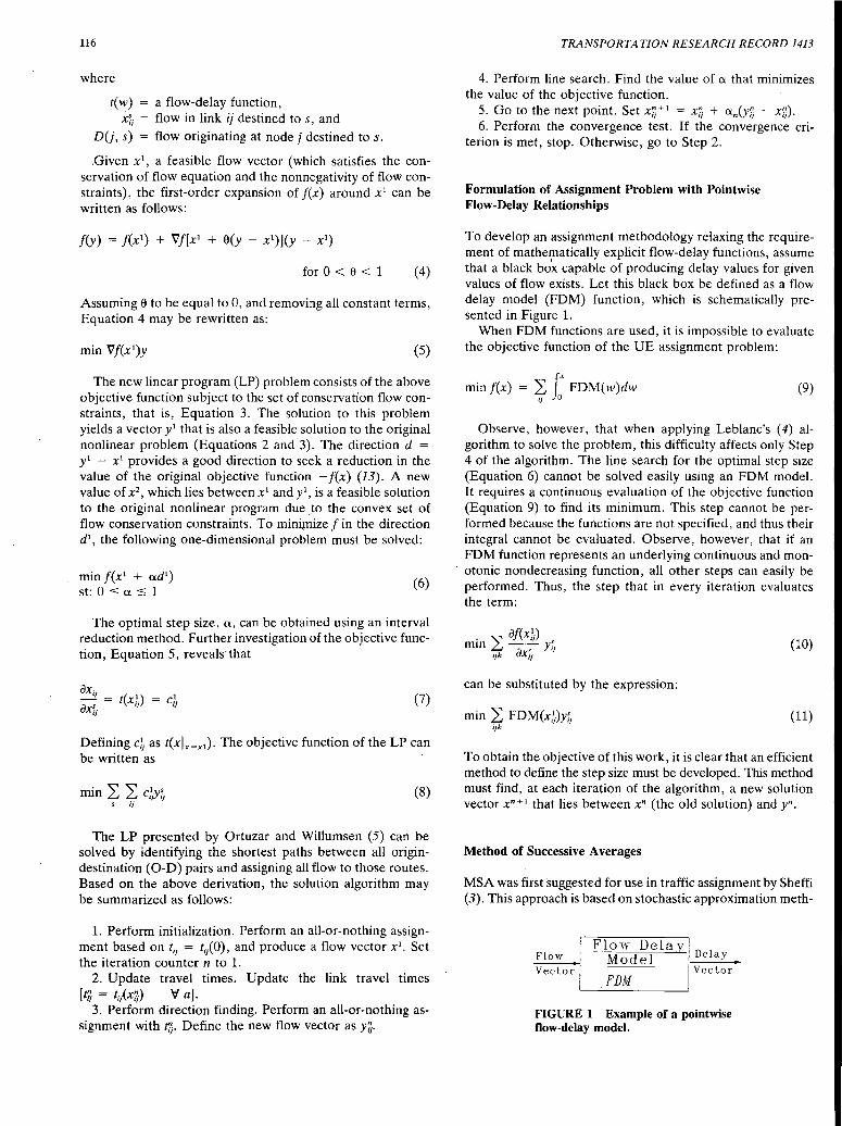
116

where

t(w) = a flow-delay function, xfj = flow in link ij destined to s' and

D(j, s) = flow originating at node j destined to s.

,Given x 1, a feasible flow vector (which satisfies the con­

servation of flow equation and the nonnegativity of flow con­straints), the first-order expansion of f(x) around x 1 can be written as follows:

f(y) = f(x 1) + Vf[x 1 + 0(y - x1)](y - x1

)

for 0 < e < 1 ( 4)

Assuming 0 to be equal to 0, and removing all constant terms, Equation 4 may be rewritten as:

min Vf(x1)y (5)

The new linear program (LP) problem consists of the above objective function subject to the set of conservation flow con­straints, that is, Equation 3. The solution to this problem yields a vector y 1 that is also a feasible solution to the original nonlinear problem (Equations 2 and 3). The direction d =

y1 - x1 provides a good direction to seek a reduction in the value of the original objective function -f(x) (13). A new value of x2

, which lies between x1 and y1, is a feasible solution

to the original nonlinear program due Jo the convex set of flow conservation constraints. To mini,nize fin the direction d1

, the following one-dimensional problem must be solved:

min f(x 1 + exd1)

st: 0 :s: ex :::;; 1 (6)

The optimal step size, ex, can be obtained using an interval reduction method. Further investigation of the objective func­tion, Equation 5, reveals-that

(7)

Defining c}j as t(xlx=x1). The objective function of the LP can be written as ·

(8)

The LP presented by Ortuzar and Willumsen (5) can be solved by identifying the shortest paths between all origin­destination (0-D) pairs and assigning all flow to those routes. Based on the above derivation, the solution algorithm may be summarized as follows:

1. Perform initialization. Perform an all-or-nothing assign­ment based on t;j = t;/O), and produce a flow vector x1

• Set the iteration counter n to 1.

2. Update travel times. Update the link travel times [ti;· = t,1(x~.) Va].

3. Perform direction finding. Perform an all-or-nothing as­signment with tij. D~fine the new flow vector as yij.

TRANSPORTATION RESEARCH RECORD 1413

4. Perform line search. Find the value of ex that minimizes the value of the objective function.

5. Go to the next point. Set xz+ 1 = Xij + exn(yij - xij). 6. Perform the convergence test. If the convergence cri­

terion is met, stop. Otherwise, go to Step 2.

Formulation of Assignment Problem with Pointwise Flow-Delay Relationships

To develop an assignment methodology relaxing the require­ment of mathematically explicit flow-delay functions, assume that a black bo~ capable of producing delay values for given values of flow exists. Let this black box be defined as a flow delay model (FDM) function, which is schematically pre­sented in Figure 1.

When FDM functions are used, it is impossible to evaluate the objective function of the UE assignment problem:

minf(x) = 4 J: FDM(w)dw lj

(9)

Observe, however, that when applying Leblanc's (4) al­gorithm to solve the problem, this difficulty affects only Step 4 of the algorithm. The line search for the optimal step size (Equation 6) cannot be solved easily using an FDM model. It requires a continuous evaluation of the objective function (Equation 9) to find its minimum. This step cannot be per­formed because the functions are not specified, and thus their integral cannot be evaluated. Observe, however, that if an FDM funCtion represents an underlying continuous and mon-

. otonic nondecreasing function, all other steps can easily be performed. Thus, the step that in every iteration evaluates the term:

. ""' af(xt) mm Li -- Y~-

ijk ar;j I}

can be substituted by the expression:

min L FDM(xt)yfj ijk

(10)

(11)

To obtain the objective of this work, it is clear that an efficient method to define the step size must be developed. This method must find, at each iteration of the algorithm, a new solution vector xn+l that lies between xn (the old solution) and yn.

Method of Successive Averages

MSA was first suggested for use in traffic assignment by Sheffi (3). This approach is based on stochastic approximation meth-

Flow

Vector

Flow Delay Model Delay

Vector FDM

FIGURE 1 Example of a pointwise flow-delay model.

Regueros et al.

ods. Stochastic approximation is concerned with the conver­gence of problems that are stochastic in nature, usually based on observations that involve errors. Search techniques that successfully reach optimum despite the stochastic noise were named "stochastic approximation methods" by Robbins and Monroe in 1954 (14). The term approximation refers, in this context, to the continual use of past measurements to estimate the approximate position of the solution, and the term sto­chastic suggests the random character of the function being evaluated.

The Robbins-Monroe procedure places solution point n + 1 as a function of the solution of point n according to the following equation:

(12)

where z(x) is a "noisy" function. The method is based on predetermined step-size series (a)

that must satisfy the following two conditions:

00

2: an~ 00

n=i

00

2: a~< oo n=l

(13)

In general, any sequence can be used that can be expressed by the equation:

Ki a=---

n Kz + n (14)

where Ki > 0 and K2 2: 0. One of the simplest step-size sequences that satisfies both conditions is the series:

1 a = -

n n (15)

Sheffi (3) applied this methodology to solve a probabilistic assignment problem. The same approach can be used to solve a deterministic assignment problem when flow-delay relations are expressed as FDM functions. The complete algorithm can be summarized as follows:

1. Perform initialization. (a) Run the simulation program with an initial flow vector. (b) Perform an all-or-nothing assignment to produce a

flow vector xi. 2. Update travel times. Perform a simulation run with flow

vector xn, generating new travel times (tjj). 3. Perform direction finding. Perform an all-or-nothing as­

signment with tjj and define the new flow vector as yij. 4. Go to the next point. Find a point xn + 1 between xn and

yn as follows:

(16)

Increase the iteration counter n. 5. Perform the convergence test. If the convergence cri­

terion is met, stop. Otherwise, go to Step 2.

117

The drawbacks and advantages of the algorithm can be attributed to the use of predetermined step sizes. The advan­tage is the simplicity of the algorithm and its insensitivity to noisy simulation results. One disadvantage is that the algo­rithm does not directly utilize information obtained with the execution of each simulation step. Thus the convergence is very slow, and appropriate convergence criteria are difficult to define (15).

·Another disadvantage of MSA may be illustrated with the following example. The MSA algorithm was applied to solve the assignment problem of a network consisting of three links and one 0-D pair (see Sheffi (3), page 114). Figure 2 shows the objective function, z(x), as a function of the iteration number. If the MSA procedure is ended after a predetermined number of iterations, a poor convergence may be achieved. This can happen because the results of each MSA iteration asymptotically oscillate around the true solution value and do not approach convergence monotonically.

Linear Approximation Method

The proposed method is based on a linear approximation of the real underlying flow-delay function. At each iteration of the Frank-Wolfe algorithm, a new flow-delay point is gen­erated for each network element and a straight line that passes through the last iteration flow-delay point and the present one is calculated. For an errorless FDM function, the straight line will always be a nondecreasing function of volume. The proposed assignment algorithm is composed of a succession of these straight lines used in conjunction with traditional Frank-Wolfe iterations. Theoretically, higher dimension-curve approximation can be developed. The storage requirement in such a case will increase significantly, and it is unclear whether the algorithm's performance will improve. Remember that the higher dimensionality curve must be nondecreasing. Thus, in some cases, the approximation may result in a poor fit. Therefore, the authors chose the simplest of all approxima­tions-a linear one. At each iteration of Frank-Wolfe's al­gorithm, only two flow-delay points are considered. At each iteration of the algorithm, a straight line is assumed to rep­resent the present flow-delay relationships. During iteration (n), the straight line passes through points xn-i and xn. Com-

215

210

_205 >< N' 200

195

190

185-+-----,----~----.----~--~ 0 10 20

Iteration

I Sheffi.Ntw. Sheffi.Dmd J I - FW --e-- MSA

FIGURE 2 Objective function, z(x), as a function of iteration number.

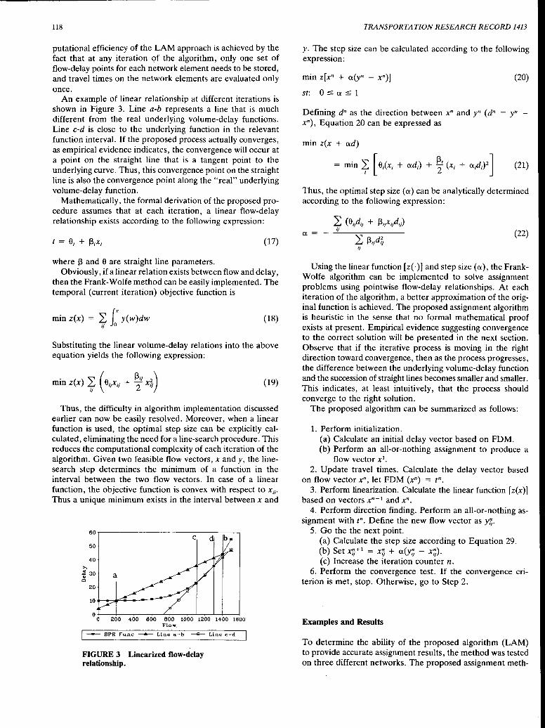
118

putational efficiency of the LAM approach is achieved by the fact that at any iteration of the algorithm, only one set of flow-delay points for each network element needs to be stored, and travel times on the network elements are evaluated only once.

An example of linear relationship at different iterations is shown in Figure 3. Line a-b represents a line that is much different from the real underlying volume-delay functions. Line c-d is close to the underlying function in the relevant function interval. If the proposed process actually converges, as empirical evidence indicates, the convergence will occur at a point on the straight line that is a tangent point to the underlying curve. Thus, this convergence point on the straight line is also the convergence point along the "real" underlying volume-delay function.

Mathematically, the formal derivation of the proposed pro­cedure assumes that at each iteration, a linear flow-delay relationship exists according to the following expression:

t = 0; + j3;X; (17)

where 13 and 0 are straight line parameters. Obviously, if a linear relation exists between flow and delay,

then the Frank-Wolfe method can be easily implemented. The temporal (current iteration) objective function is

min z(x) = 4,: J: y(w)dw lj

(18)

Substituting the linear volume-delay relations into the above equation yields the following expression:

. ( ) " (e 13ij 2) mm z x f iixii + 2 X;i (19)

Thus, the difficulty in algorithm implementation discussed earlier can now be easily resolved. Moreover, when a linear function is used, the optimal step size can be explicitly cal­culated, eliminating the need for a line-search procedure. This reduces the computational complexity of each iteration of the algorithm. Given two feasible flow vectors, x and y, the line­search step determines the minimum of a function in the interval between the two flow vectors. In case of a linear function, the objective function is convex with respect to X;i·

Thus a unique minimum exists in the interval between x and

50

40

20

200 400 600 800 1000 1200 1400 1600 Flow.

I - BPR Fune - Line a-b -e- Line c-d

FIGURE 3 Linearized flow-delay relationship.

TRANSPORTATION RESEARCH RECORD 1413

y. The step size can be calculated according to the following expression:

(20)

st: 0 ::; ex ::; 1

Defining dn as the direction between xn and yn ( dn = yn -xn), Equation 20 can be expressed as

min z(x + ad)

~ min~ [ O;(x, + ad,) + % (x, + a,d,)'] (21)

Thus, the optimal step size (ex) can be analytically determined according to the following expression:

2: 13ijdi (22)

ij

Using the linear function [z(·)] and step size (ex), the Frank­Wolfe algorithm can be implemented to solve assignment problems using pointwise flow-delay relationships. At each iteration of the algorithm, a better approximation of the orig­inal function is achieved. The proposed assignment algorithm is heuristic in the sense that no formal mathematical proof exists at present. Empirical evidence suggesting convergence to the correct solution will be presented in the next section. Observe that if the iterative process is moving in the right direction toward convergence, then as the process progresses, the difference between the underlying volume-delay function and the succession of straight lines becomes smaller and smaller. This indicates, at least intuitively, that the process should converge to the right solution.

The proposed algorithm can be summarized as follows:

1. Perform initialization. (a) Calculate an initial delay vector based on FDM. (b) Perform an all-or-nothing assignment to produce a

flow vector x 1•

2. Update travel times. Calculate the delay vector based on flow vector xn, let FDM (xn) = rn.

3. Perform linearization. Calculate the linear function [z(x)] based on vectors xn - 1 and xn.

4. Perform direction finding. Perform an all-or-nothing as­signment with in. Define the new flow vector as yij.

5. Go the the next point. (a) Calculate the step size according to Equation 29. (b) Set xij+ 1 = xij + a(yij - xij). (c) Increase the iteration counter n.

6. Perform the convergence test. If the convergence cri­terion is met, stop. Otherwise, go to Step 2.

Examples and Results

To determine the ability of the proposed algorithm (LAM) to provide accurate assignment results, the method was tested on three different networks. The proposed assignment meth-

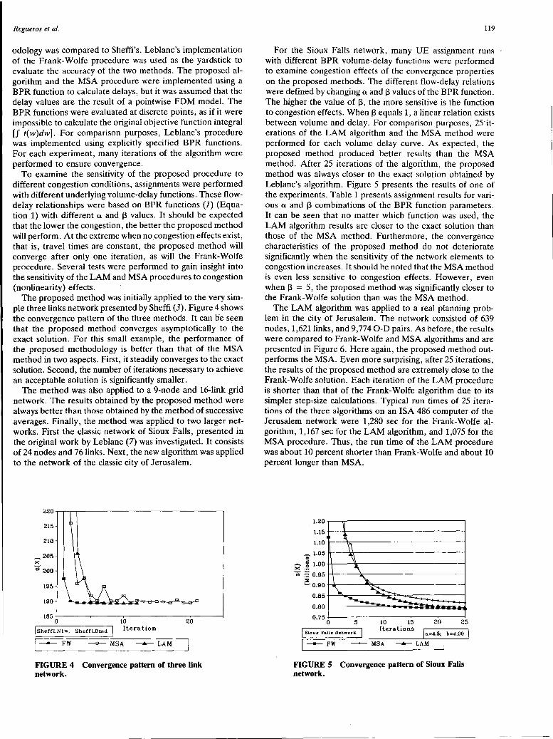
Regueros et al.

odology was compared to Sheffi's. Leblanc's implementation of the Frank-Wolfe procedure was used as the yardstick to evaluate the accuracy of the two methods. The proposed al­gorithm and the MSA procedure were implemented using a BPR function to calculate delays, but it was assumed that the delay values are the result of a pointwise FDM model. The BPR functions were evaluated at discrete points, as if it were impossible to calculate the original objective function integral [f t(w)dw]. For comparison purposes, Leblanc's procedure was implemented using explicitly specified BPR functions. For each experiment, many iterations of the algorithm were performed to ensure convergence.

To examine the sensitivity of the proposed procedure to different congestion conditions, assignments were performed with different underlying volume-delay functions. These flow­delay relationships were based on BPR functions (1) (Equa­tion 1) with different a and J3 values. It should be expected that the lower the congestion, the better the proposed method will perform. At the extreme when no congestion effects exist, that is, travel times are constant, the proposed method will converge after only one iteration, as will the Frank-Wolfe procedure. Several tests were performed to gain insight into the sensitivity of the LAM and MSA procedures to congestion (nonlinearity) effects.

The proposed method was initially applied to the very sim­ple three links network presented by Sheffi (3). Figure 4 shows the convergence pattern of the three methods. It canoe s~en that the proposed method converges asymptotically to the exact solution. For this small example, the performance of the proposed methodology is better than that of the MSA method in two aspects. First, it steadily converges to the exact solution. Second, the number of iterations necessary to achieve an acceptable solution is significantly smaller.

The method was also applied to a 9-node and 16-link grid network. The results obtained by the proposed method were always better than those obtained by the method of successive averages. Finally, the method was applied to two larger net­works. First the classic network of Sioux Falls, presented in the original work by Leblanc (7) was investigated. It consists of 24 nodes and 76 links. Next, the new algorithm was applied to the network of the classic city of Jerusalem.

215

210

_205 >< 'N 200

195

190

185+---~---~--~---~---1 0

isheffi.Nt>V, Sheffi.Dmd

10 Iteration

1-Fw -e- MSA ___.._ LAM

20

FIGURE 4 Convergence pattern of three link network.

119

For the Sioux Falls network, many UE assignment runs J

with different BPR volume-delay functions were performed to examine congestion effects of the convergence properties on the proposed methods. The different flow-delay relations were defined by changing a and J3 values of the BPR function. The higher the value of J3, the more sensitive is the function to congestion effects. When J3 equals 1, a linear relation exists between volume and delay. For comparison purposes, 25'it­erations of the LAM algorithm and the MSA method were performed for each volume delay curve. As expected, the proposed method produced better results than the MSA method. After 25 iterations of the algorithm, the proposed method was always closer to the exact solution obtained by Leblanc's algorithm. Figure 5 presents the results of one of the experiments. Table 1 presents assignment results for vari­ous a and J3 combinations of the BPR function parameters. It can be seen that no matter which function was used, the LAM algorithm results are closer to the exact solution tha·n those of the MSA method. Furthermore, the convergence characteristics of the proposed method do not deteriorate significantly when the sensitivity of the network elements to congestion increases. It should be noted that the MSA method is even less sensitive to congestion effects. However, even when J3 = 5, the proposed method was significantly closer to the Frank-Wolfe solution than was the MSA method.

The LAM algorithm was applied to a real planning prob­lem in the city of Jerusalem. The network consisted of 639 nodes, 1,621 links, and 9,774 0-D pairs. As before, the results were compared to Frank-Wolfe and MSA algorithms and are presented in Figure 6. Here again, the proposed method out­performs the MSA. Even more surprising, after 25 iterations, the results of the proposed method are extremely close to the Frank-Wolfe solution. Each iteration of the LAM procedure is shorter than that of the Frank-Wolfe algorithm due to its simpler step.,.size calculations. Typical run times of 25 itera­tions of the three algorithms on an ISA 486 computer of the Jerusalem network were 1,280 sec for the Frank-Wolfe al­gorithm, 1,167 sec for the LAM algorithm, and 1,075 for the MSA procedure. Thus, the run time of the LAM procedure was about 10 percent shorter than Frank-Wolfe and about 10 percent longer than MSA.

1.20..------n--------------,

1.15 +----ll-------------;

1.10 +--~------------1

- 1.05 ~---i.-.-------------; Gil .

>< .2 1.00 'N ; 0.95 ++----2------------1

::i; - 0.90 +-.---~::-----------j

0.85 +--=.o::=---.=,.~,,.....-=;;;::-:-------j

0.80 +----.=-=:m:t!......,_w=ii~~~--:fii':i

0·75 o +----5....--~10---.~5---2~0---l25

j Sioux Falls Network I Iterations a=4.5; b=4.00

-FW --+- MSA ___.....__ LAM

FIGURES Convergence pattern of Sioux Falls network.

120 TRANSPORTATION RESEARCH RECORD 1413

TABLE 1 Objective Function Values for Sioux Falls Network

Parameter Method

a 13 FW MSA

0.15 1 673465.25 673465.06 0.15 2 658047.13 658092.72 0.15 3 652008.50 652094.23 0.15 4 649040.33 649380.82 0.15 5 647383.66 647816.21 3.00 1 1251805.93 ' 1262714.46 3.00 2 920306.65 938585.44 3.00 3 797500.07 814918.08 3.00 4 741256.24 756196.98 3.00 5 711110.66 732911.87 4.50 1 1052317.34 1081560.57 4.50 2 1052317.34 1081560.57 4.50 3 868625.09 4.50 4 784554.39 4.50 5 742024.08

17-r---.--,.,..---------------.

16.9 +--+~+--------------! r-i

~ 16.8 +-__._+-+------------~ 0 ::: 16.7 +---lm-'l-_,,._------------1

i 16.6 +-----..-_,,,.__-=-------------l ,..--. 16.5 +----~~--=-------------l

C- 16.4+------~~;::-:--------~ N

895160.58 812435.01 769401.7

16.2 +-----.-------.------.-----.----=-'1 0 5 10 15 20 25

Iteration

1- FW ---+--- MSA ___..,_ LAM

FIGURE 6 Results of Jerusalem network.

CONCLUSIONS

The proposed linear approximation assignment method ap­pears to work well. When an errorless deterministic FDM exists, the proposed method is clearly superior to the MSA method in its convergence properties. An advantage of the proposed method is that it provides an elegant, simple, and computer-storage-efficient iterative procedure to combine traffic assignment with simulation results. Another significant char­acteristic of the proposed method is that its convergence char­acteristics are not sensitive to congestion effects.

The proposed method can easily be adapted to situations in which some of the network elements are represented by aggregate flow-delay curves, and the behavior of others is determined by FDM functions. The need to combine two types of volume-delay functions arises when the behavior of some network elements is too complicated to be represented by an aggregate function. When performing microassignment or assignment used to support traffic control decisions, net­work elements, such as intersection approaches, weaving sec­tions, ramps, and other similar elements, need to be repre­sented in detail. On the other hand, many elements do not need such a fine representation. Furthermore, this method also seems well suited to be applied as a second-stage refined

Results (percent)

LAM FW-MSA FW-LAM

673465.42 0.0000 0.0000 658048.79 0.0069 0.0003 652008.11 0.0131 -0.0001 649056.72 0.0525 0.0025 647397.8 0.0668 0.0022

1251836.66 0.8714 0.0025 920602.65 1.9862 0.0322 800769.58 2.1841 0.4100 744504.26 2.0156 0.4382 713986.46 3.0658 0.4044

1054371.86 2.7789 0.1952 1054371.86 2.7789 0.1952 873920.02 3.0549 0.6096 790197.29 3.5537 0.7192 748640.45 3.5896 0.8917

assignment procedure to a solution vector that was generated from aggregate flow-delay functions.

Procedures that perform stochastic assignment are of great interest. The ability of the proposed procedure to perform stochastic assignment was not fully investigated. When the method is applied to solve stochastic assignment problems, the slope of the flow-delay line, in some iterations, may be negative. This violates one of the properties necessary for the convergence of the Frank-Wolfe algorithm. However, due to the stochastic properties of the process, the slope will be negative only during part of the iterations. Thus it may, al­though not necessarily will, imperil the convergence of the procedure. A probable way to overcome the problem is to assign a zero slope, or to use the slope value of the previous iteration. The probability that the slope will be negative in­creases as the distance between the two points defining the straight line decreases and as the gradient of the underlying flow-delay curve between the two points approaches zero. Due to the complexity of the convergence process of stochastic assignment, the convergence characteristics· of the proposed method when performing stochastic assignment needs further investigation.

ACKNOWLEDGMENTS

This research was supported by a grant from the Israel Min­istry of Transport. Special thanks are due to Lyn Long of the University of California, Irvine, for reviewing and editing this paper.

REFERENCES

1. Traffic Assignment Manual, Bureau of Public Roads, Urban Plan­ning Division, U.S. Department of Commerce, 1964.

2. Hall, M. D., D. Van Vliet, and L. G. Willumsen. SATURN­A Simulation-Assignment Model for the Evaluation of Traffic Management Schemes. Traffic Engineering & Control, 1980, pp. 168-175.

3. Sheffi, Y. Urban Transportation Networks: Equilibrium Analysis with Mathematical Programming Methods. Prentice-Hall, Inc., Englewood Cliffs, N.J., 1985.

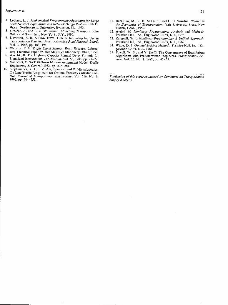
Regueros et al.

4. Leblanc, L. J. Mathematical Programming Algorithms for Large Scale Network Equilibrium and Network Design Problems. Ph.D. thesis. Northwestern University, Evanston, Ill., 1973.

5. Ortuzar, J., and L. G. Willumsen. Modelling Transport. John Wiley and Sons, Inc., New York, N.Y., 1990.

6. Davidson, K. B. A Flow Travel Time Relationship for Use in Transportation Planning. Proc., Australian Road Research Board, Vol. 3, 1966, pp. 183-194.

7. Webster, F. V. Traffic Signal Settings. Road Research Labora­tory Technical Paper 39. Her Majesty's Stationery Office, 1958.

8. Akcelik, R. The Highway Capacity Manual Delay Formula for Signalized Intersections. !TE Journal, Vol. 58, 1988, pp. 23-27.

9. Van Vliet, D. SATURN-A Modern Assignment Model. Traffic Engineering & Control, 1982, pp. 578-581.

10. Stephanedes, Y. J., I. Z. Argiropoulos, and P. Michalopoulos. On-Line Traffic Assignment for Optimal Freeway Corridor Con­trol. Journal of Transportation Engineering, Vol. 116, No. 6, 1990, pp. 744-755.

121

11. Beckman, M., C. B. McGuire, and C. B. Winston. Studies in the Economics of Transportation. Yale University Press, New Haven, Conn., 1956.

12. Avriel, M. Nonlinear Programming: Analysis and Methods. Prentice-Hall, Inc., Englewood Cliffs, N.J., 1976.

13. Zangwill, W. I. Nonlinear Programming: A Unified Approach. Prentice-Hall, Inc., Englewood Cliffs, N.J., 1969.

14. Wilde, D. J. Optimal Seeking Methods. Prentice-Hall, Inc., En­glewood Cliffs, N.J., 1964.

15. Powell, W. B., and Y. Sheffi. The Convergence of Equilibrium Algorithms with Predetermined Step Sizes. Transportation Sci­ence, Vol. 16, No. 1, 1982, pp. 45-55.

Publication of this paper sponsored by Committee on Transportation Supply Analysis.

122 TRANSPORTATION RESEARCH RECORD 1413

Properties of Vehicle Routes with Variable Shipment Sizes in Euclidean Plane RANDOLPH w. HALL

A fundamental limitation of the literature on continuous-space routin~ models is that vehicles are assumed to have a capacity for a fixed number of stops. In reality, the maximum number of stops on a route may be defined by how well shipments pack into av~ilable capacities. An exploratory study of the geometric prop­erties ?f ve?~cle ~outes that carry shipments of variable size (hence, ~apac1ty utihzation and number of stops vary from route to route) is presented. Instead of taking a purely theoretical approach, the study relies on ~n empirical analysis of routing solutions to reveal the properties of near-optimal routes. Route geometry is then explained with a "theory of spokes," where a spoke is a line segment connecting the terminal to the most distant stop on a route. Because the number of spokes per unit circumference in­creases in the vicinity of the terminal, the incremental distance of serving a stop is a nonlinear function of distance to the terminal. Because of packing considerations, the incremental distance is also a nonlinear function of shipment size.

The classic vehicle routing problem (VRP) entails creating a set of routes of minimum total length so that each available stop is visited and vehicle loads do not violate constraints on capacity or time. The VRP has a long research history, be­ginning with the work of Dantzig and Ramser in 1959 (1). Research on the VRP is summarized by Bodin et al. (2), LaPorte and Nobert (3), and Magnanti (4), along with the book edited by Golden and Assad (5).

A number of researchers have used continuous-space models to study the theoretical behavior and geometric properties of VRP solutions. Most notable are the works by Daganzo (6,7) and Newell and Daganzo (8). These build from earlier models for the traveling salesman problem by Beardwood et al. (9), Few (10), Stein (11), and Verblunsky (12), and empirical work on the VRP by Christofides and Eilon (13). The accomplish­ment of Daganzo and Newell was to develop a theory of near­optimal route geometry and expected route length in Euclid­ean space. Haimovich and Rinnooy Kan (14); Haimovich, Rinnooy Kan, and Stougie (15); and Spaccamela, Rinnooy Kan, and Stougie (16) have also produced bounds on the length of VRP routes in Euclidean space as part of their effort to evaluate the asymptotic performance of routing heuristics.

More recently, routes with mixed pickups and deliveries have been studied by Daganzo and Hall (17) and Hall (18). The latter identifies the optimal shape and orientation of routes that begin and end at different terminals. The former studies mixed pickup and delivery routes out of a single terminal.

D.epartment of Industrial Engineering and Operations Research, In­stit~te of Transportatio~ ~t~dies, University of California, Berkeley, Cali~. 94720; current affihation: Department of Information and Op­erations Management, School of Business Administration, University of Southern California, Los Angeles, Calif. 90089-1421.

The work by Daganzo and Hall (17) is significant in that it introduces the concept of line-haul spokes, which are used in this paper to explain the effects of capacity utilization on route length. Also, research has recently been completed on ·dy­namic routing, where the presence of stops or characteristics of shipments, or both, are not revealed until the vehicle is in motion (19-21).

A fundamental limitation of the continuous-space literature is that vehicles are assumed to have a capacity for a fixed number of stops. In reality, the maximum number of stops may be defined by how well shipments pack into available capacities (e.g., weight of time). And because shipments do not have to be identical, the number of stops and the capacity utilization can vary from route to route. For instance, if split­ting shipments among routes is not allowed, then solving the VRP depends in part on the solution to a bin-packing prob­lem. However, unlike the classic bin-packing problem, the objective is not simply to minimize the number of bins, but is instead to minimize the product of the number of bins (i.e., routes) and the average length per route. The latter depends on the dispersion of stops on routes.

As discussed by Hall et al. (22), the two goals of minimizing the number of routes and the average length per route conflict with each other because efficient packings may demand non­compact routes. This trade-off is most prominent when ship­ments tend to be large relative to vehicle capacity.

Though the theoretical properties of bin-packing algorithms are well known (23) and the geometric properties of vehicle routes with a fixed number of stops are well known, little research had been completed on the geometric properties of vehicle routes with variable shipment sizes. (There is, how­ever, an extensive body of literature on algorithms for solving vehicle routing problems with variable shipment sizes.) Hall and Daganzo (24) examined route characteristics when ve­hicles are limited by weight and volume constraints with in­finitely divisible commodities. Hall (25) studied the trade-off between packing efficiency and average route length under a scheme whereby sets of vehicles are allowed to cove identical territories. However, this scheme is surely inferior to partially overlapped territories.

The introduction of variable shipment sizes motivates changes in route structure as well as changes in the relationship be­tween route length and stop density. The objective of this paper is to develop an understanding of how variations in shipment size affect optimal route length and optimal route geometry.

Although this research entails testing algorithms, algorithm development is not a primary goaL The intention is to begin the development of an empirically based theory of routing

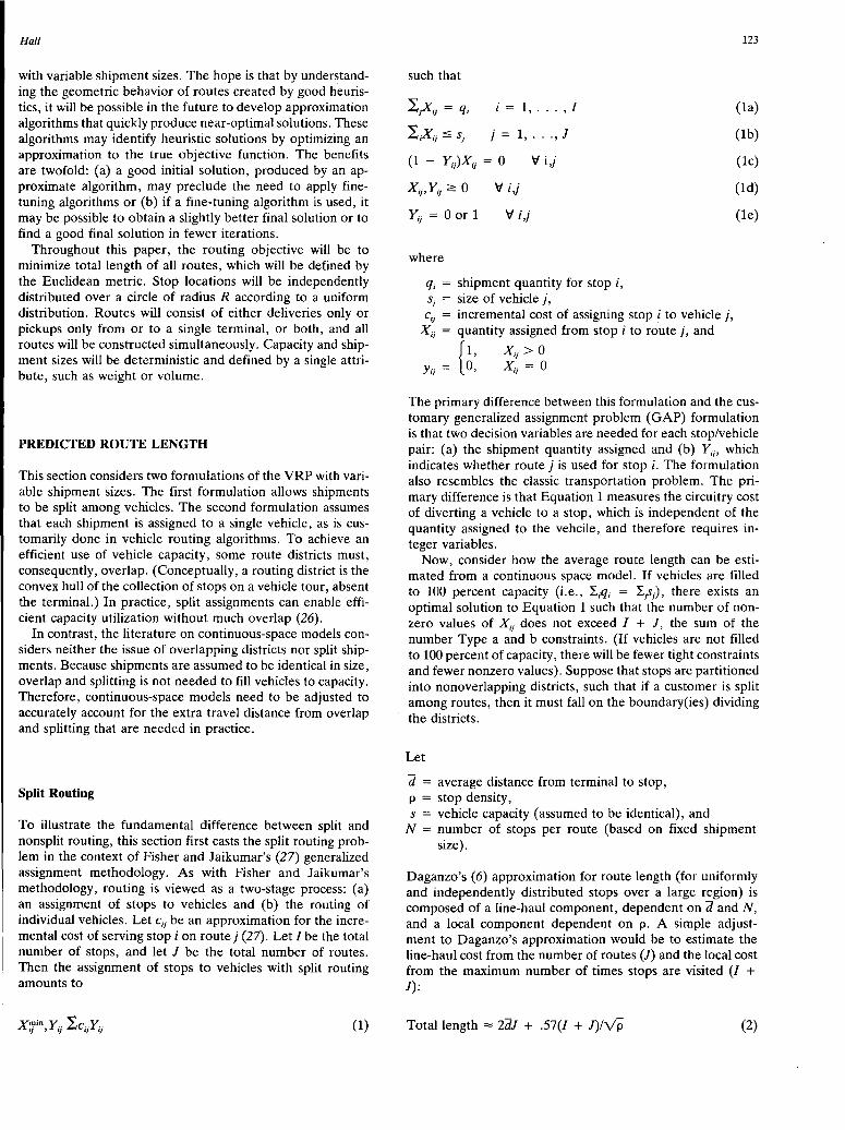
Hall

with variable shipment sizes. The hope is that by understand­ing the geometric behavior of routes created by good heuris­tics, it will be possible in the future to develop approximation algorithms that quickly produce near-optimal solutions. These algorithms may identify heuristic solutions by optimizing an approximation to the true objective function. The benefits are twofold: (a) a good initial solution, produced by an ap­proximate algorithm, may preclude the need to apply fine­tuning algorithms or (b) if a fine-tuning algorithm is used, it may be possible to obtain a slightly better final solution or to find a good final solution in fewer iterations.

Throughout this paper, the routing objective will be to minimize total length of all routes, which will be defined by the Euclidean metric. Stop locations will be independently distributed over a circle of radius R according to a uniform distribution. Routes will consist of either deliveries only or pickups only from or to a single terminal, or both, and all routes will be constructed simultaneously. Capacity and ship­ment sizes will be deterministic and defined by a single attri­bute, such as weight or volume.

PREDICTED ROUTE LENGTH

This section considers two formulations of the VRP with vari­able shipment sizes. The first formulation allows shipments to be split among vehicles. The second formulation assumes that each shipment is assigned to a single vehicle, as is cus­tomarily done in vehicle routing algorithms. To achieve an efficient use of vehicle capacity, some route districts must, consequently, overlap. (Conceptually, a routing district is the convex hull of the collection of stops on a vehicle tour, absent the terminal.) In practice, split assignments can enable effi­cient capacity utilization without much overlap (26).

In contrast, the literature on continuous-space models con­siders neither the issue of overlapping districts nor split ship­ments. Because shipments are assumed to be identical in size, overlap and splitting is not needed to fill vehicles to capacity. Therefore, continuous-space models need to be adjusted to accurately account for the extra travel distance from overlap and splitting that are needed in practice.

Split Routing

To illustrate the fundamental difference between split and nonsplit routing, this section first casts the split routing prob­lem in the context of Fisher and J aikumar's (27) generalized assignment methodology. As with Fisher and Jaikumar's methodology, routing is viewed as a two-stage process: (a) an assignment of stops to vehicles and (b) the routing of individual vehicles. Let cii be an approximation for the incre­mental cost of serving stop ion route j (27). Let I be the total number of stops, and let J be the total number of routes. Then the assignment of stops to vehicles with split routing amounts to

(1)

such that

l ;Xii = qi i = 1, . . . , I

l;Xii ~Si j = 1, .. ., J

(1 - Yi)Xii = 0 'V i,j

Yii = 0 or 1 'V i ,j

where

qi = shipment quantity for stop i, si = size of vehicle j,

c;i = incremental cost of assigning stop ! to vehicle j, X;i = quantity assigned from stop i to route j, and

{1, xij > o

Yii = 0, Xii = 0

123

(la)

(lb)

(le)

(ld)

(le)

The primary difference between this formulation and the cus­tomary generalized assignment problem (GAP) formulation is that two decision variables are needed for each stop/vehicle pair: (a) the shipment quantity assigned and (b) Y;i, which indicates whether route j is used for stop i. The formulation also resembles the classic transportation problem. The pri­mary difference is that Equation 1 measures the circuitry cost of diverting a vehicle to a stop, which is independent of the quantity assigned to the vehcile, and therefore requires in­teger variables.

Now, consider how the average route length can be esti­mated from a continuous space model. If vehicles are filled to 100 percent capacity (i.e., !,iqi = IfJ, there exists an optimal solution to Equation 1 such that the number of non­zero values of X;i does not exceed I + J, the sum of the number Type a and b constraints. (If vehicles are not filled to 100 percent of capacity, there will be fewer tight constraints and fewer nonzero values). Suppose that stops are partitioned into nonoverlapping districts, such that if a customer is split among routes, then it must fall on the boundary(ies) dividing the districts.

Let

d = average distance from terminal to stop, p = stop density, s = vehicle capacity (assumed to be identical), and

N = number of stops per route (based on fixed shipment size).

Daganzo's (6) approximation for route length (for uniformly and independently distributed stops over a large r~gion) is . composed of a line-haul component, dependent on d and N, and a local component dependent on p. A simple adjust­ment to Daganzo's approximation would be to estimate the line-haul cost from the number of routes (J) and the local cost from the maximum number of times stops are visited (I + J):

Total length = 2dJ + .57(/ + J)/yp (2)

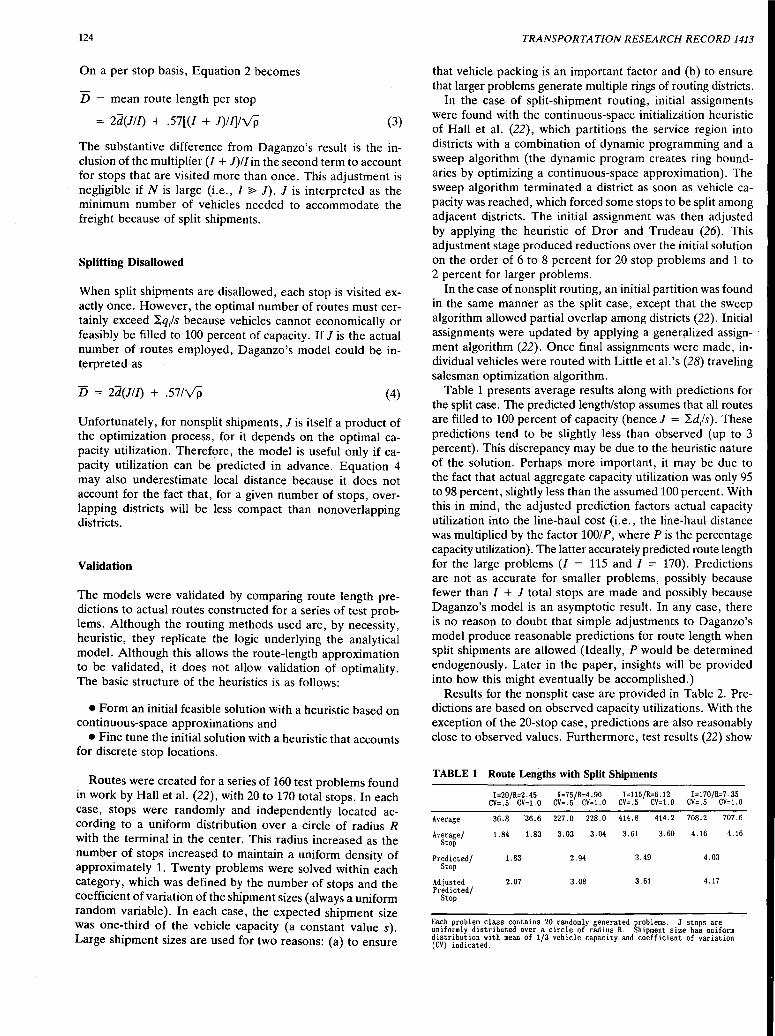
124

On a per stop basis, Equation 2 becomes

D = mean route length per stop

= 2d(J!J) + .57[(/ + J)!l]!yp (3)

The substantive difference from Daganzo's result is the in­clusion of the multiplier (I + J)! I in the second term to account for stops that are visited more than once. This adjustment is negligible if N is large (i.e., I ~ J). J is interpreted as the minimum number of vehicles needed to accommodate the freight because of split shipments.

Splitting Disallowed

When split shipments are disallowed, each stop is visited ex­actly once. However, the optimal number of routes must cer­tainly exceed "'iq/s because vehicles cannot economically or feasibly be filled to 100 percent of capacity. If J is the actual number of routes employed, Daganzo's model could be in­terpreted as

15 = 2d(J!J) + .57/yp (4)

Unfortunately, for nonsplit shipments, J is itself a product of the optimization process, for it depends on the optimal ca­pacity utilization. Theref~re, the model is useful only if ca­pacity utilization can be predicted in advance. Equation 4 may also underestimate local distance because it does not account for the fact that, for a given number of stops, over­lapping districts will be less compact than nonoverlapping districts.

Validation

The models were validated by comparing route length pre­dictions to actual routes constructed for a series of test prob­lems. Although the routing methods used are, by necessity, heuristic, they replicate the logic underlying the analytical model. Although this allows the route-length approximation to be validated, it does not allow validation of optimality. The basic structure of the heuristics is as follows:

•Form an initial feasible solution with a heuristic based on continuous-space approximations and

• Fine tune the initial solution with a heuristic that accounts for discrete stop locations.

Routes were created for a series of 160 test problems found in work by Hall et al. (22), with 20 to 170 total stops. In each case, stops were randomly and independently located ac­cording to a uniform distribution over a circle of radius R with the terminal in the center. This radius increased as the numbe~ of stops increased to maintain a uniform density of approximately 1. Twenty problems were solved within each category, which was defined by the number of stops and the coefficient of variation of the shipment sizes (always a uniform random variable). In each case, the expected shipment size was one-third of the vehicle capacity (a constant value s). Large shipment sizes are used for two reasons: (a) to ensure

TRANSPORTATION RESEARCH RECORD 1413

that vehicle packing is an important factor and (b) to ensure that larger problems generate multiple rings of routing districts.

In the case of split-shipment routing, initial assignments were found with the continuous-space initialization heuristic of Hall et al. (22), which partitions the service region into districts with a combination of dynamic programming and a sweep algorithm (the dynamic program creates ring bound­aries by optimizing a continuous-space approximation). The sweep algorithm terminated a district as soon as vehicle ca­pacity was reached, which forced some stops to be split among adjacent districts. The initial assignment was then adjusted by applying the heuristic of Dror and Trudeau (26). This adjustment stage produced reductions over the initial solution on the order of 6 to 8 percent for 20 stop problems and 1 to 2 percent for larger problems.

In the case of nonsplit routing, an initial partition was found in the same manner as the split case, except that the sweep algorithm allowed partial overlap among districts (22). Initial assignments were updated by applying a generalized assign- · ment algorithm (22). Once final assignments were made, in­dividual vehicles were routed with Little et al. 's (28) traveling salesman optimization algorithm.

Table 1 presents average results along with predictions for the split case. The predicted length/stop assumes that all routes are filled to 100 percent of capacity (hence J = "'id/s). These predictions tend to be slightly less than observed (up to 3 percent). This discrepancy may be due to the heuristic nature of the solution. Perhaps more important, it may be due to the fact that actual aggregate capacity utilization was only 95 to 98 percent, slightly less than the assumed 100 percent. With this in mind, the adjusted prediction factors actual capacity utilization into the line-haul cost (i.e., the line-haul distance was multiplied by the factor 100/ P, where P is the percentage capacity utilization). The latter accurately predicted route length for the large problems (/ = 115 and I = 170). Predictions are not as accurate for smaller problems, possibly because fewer than I + J total stops are made and possibly because Daganzo's model is an asymptotic result. In any case, there is no reason to doubt that simple adjustments to Daganzo's model produce reasonable predictions for route length when split shipments are allowed (Ideally, P would be determined endogenously. Later in the paper, insights will be provided into how this might eventually be accomplished.)

Results for the nonsplit case are provided in Table 2. Pre­dictions are based on observed capacity utilizations. With the exception of the 20-stop case, predictions are also reasonably close to observed values. Furthermore, test results (22) show

TABLE 1 Route Lengths with Split Shipments

I =20 /R=2 . 45 CV=.5 CV=1.0

1=75/R=4. 90 CV=.5 CV=1.0

I=115/R=6.12 CV=.5 CV=l.0

1=170/R=7 .35 CV=.5 CV=LO

Average 36.8 "36.6 227 .o 228.0 414.8 414.2 708.2 707.6

Average/ 1.84 1.83 3.03 3.04 3.61 3.60 4.16 4.16 Stop

Predicted/ Stop

1.83 2.94 3.49 4.03

Adjusted 2.07 3.08 3.61 4.17 Predicted/

Stop

Ea~h proble'!' cl~s contains 20. randomly ge~erated pr<?blems. J stops are uniformly distributed over a circle of radius R. Shipment size has uniform distribution with mean of 1/3 vehicle capacity and coefficient of variation (CV) indicated.

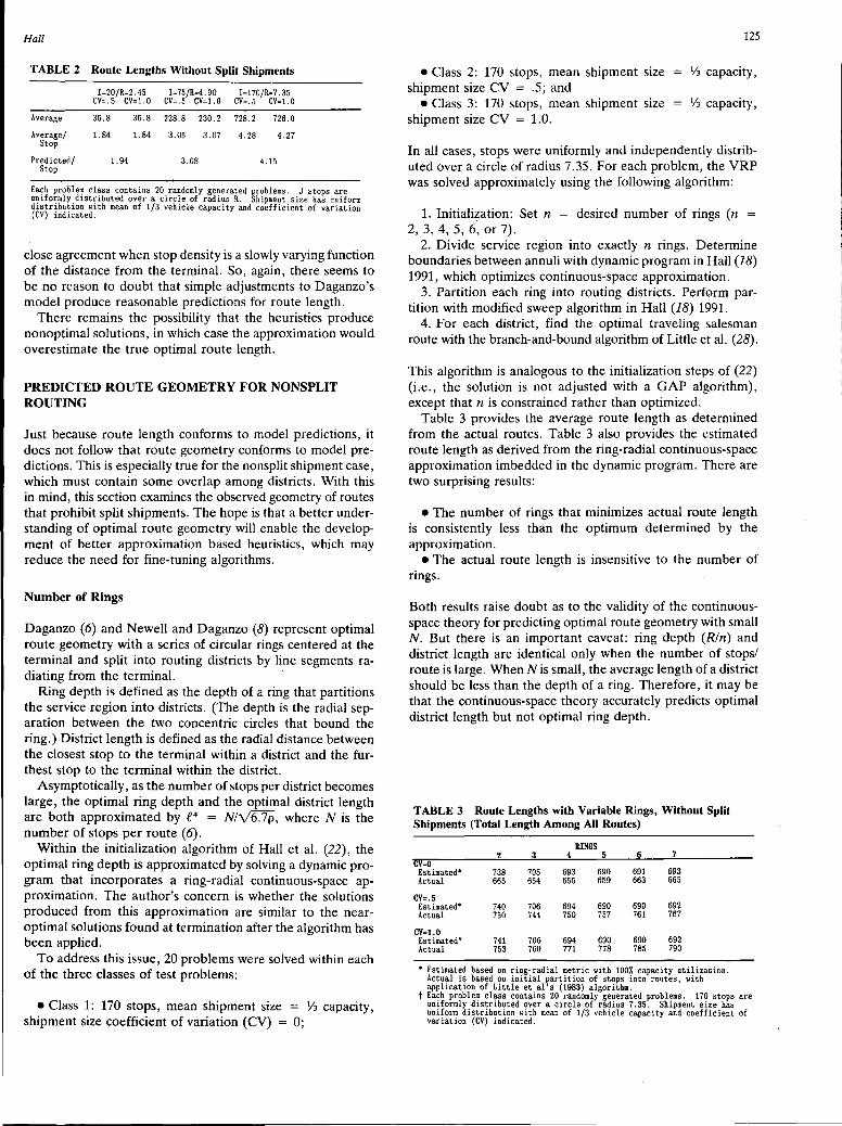
Hall

TABLE 2 Route Lengths Without Split Shipments

Average

Average/ Stop

Predicted/ Stop

I=20/R=2.45 l=75/R=4.90 I=170/R=7.35 CV=.5 CV=l.0 CV=.5 CV=l.0 CV=.5 CV=l.0

36.8

1.84

1.94

36.8 228.8 230.2 728.2 726.0

1.84 3.05 3.07 4.28 4.27

3.08 4.15

Ea~h proDie~ cll!-ss contains 20. randomly ge~erated problems. J stops are uniformly distributed over a circle of radius R. Shipment size has uniform distribution with mean of 1/3 vehicle capacity and coefficient of variation (CV) indicated.

close agreement when stop density is a slowly varying function of the distance from the terminal. So, again, there seems to be no reason to doubt that simple adjustments to Daganzo's model produce reasonable predictions for route length.

There remains the possibility that the heuristics produce nonoptimal solutions, in which case the approximation would overestimate the true optimal route length.

PREDICTED ROUTE GEOMETRY FOR NONSPLIT ROUTING

Just because route length conforms to model predictions, it does not follow that route geometry conforms to model pre­dictions. This is especially true for the nonsplit shipment case, which must contain some overlap among districts. With this in mind, this section examines the observed geometry of routes that prohibit split shipments. The hope is that a better under­standing of optimal route geometry will enable the develop­ment of better approximation based heuristics, which may reduce the need for fine-tuning algorithms.

Number of Rings

Daganzo (6) and Newell and Daganzo (8) represent optimal route geometry with a series of circular rings centered at the terminal and split into routing districts by line segments ra-diating from the terminal. ,

Ring depth is defined as the depth of a ring that partitions the service region into districts. (The depth is the radial sep­aration between the two concentric circles that bound the ring.) District length is defined as the radial distance between the closest stop to the terminal within a district and the fur­thest stop to the terminal within the district.

Asymptotically, as the number of stops per district becomes large, the optimal ring depth and the optimal district length are both approximated by f* = Nl'\/6:!P, where N is the number of stops per route ( 6).

Within the initialization algorithm of Hall et al. (22), the optimal ring depth is approximated by solving a dynamic pro­gram that incorporates a ring-radial continuous-space ap­proximation. The author's concern is whether the solutions produced from this approximation are similar to the near­optimal solutions found at termination after the algorithm has been applied.

To address this issue, 20 problems were solved within each of the three classes of test problems:

• Class 1: 170 stops, mean shipment size = % capacity, shipment size coefficient of variation (CV) = O;

125

•Class 2: 170 stops, mean shipment size shipment size CV = .5; and

% capacity,

•Class 3: 170 stops, mean shipment size shipment size CV = 1.0.

% capacity,

In all cases, stops were uniformly and independently distrib­uted over a circle of radius 7.35. For each problem, the VRP was solved approximately using the following algorithm:

1. Initialization: Set n = desired number of rings (n 2, 3, 4, 5, 6, or 7).

2. Divide service region into exactly n rings. Determine boundaries between annuli with dynamic program in Hall (18) 1991, which optimizes continuous-space approximation.

3. Partition each ring into routing districts. Perform par­tition with modified sweep algorithm in Hall (18) 1991.

4. For each district, find the optimal traveling salesman route with the branch-and-bound algorithm of Little et al. (28).

This algorithm is analogous to the initialization steps of (22) (i.e., the solution is not adjusted with a GAP algorithm), except that n is constrained rather than optimized.

Table 3 provides the average route length as determined from the actual routes. Table 3 also provides the estimated route length as derived from the ring-radial continuous-space approximation imbedded in the dynamic program. There are two surprising results:

• The number of rings that minimizes actual route length is consistently less than the optimum determined by the approximation.

• The actual route length is insensitive to the number of rings.

Both results raise doubt as to the validity of the continuous­space theory for predicting optimal route geometry with small N. But there is an important caveat: ring depth (Rln) and district length are identical only when the number of stops/ route is large. When N is small, the average length of a district should be less than the depth of a ring. Therefore, it may be that the continuous-space theory accurately predicts optimal district length but not optimal ring depth.

TABLE 3 Route Lengths with Variable Rings, Without Split Shipments (Total Length Among All Routes)

RINGS 3 4 5 6 7

=()

Estimated* 738 705 693 690 691 693 Actual 665 654 655 659 663 665

CV=.5 Estimated* 740 706 694 690 690 692 Actual 750 744 750 757 761 767

CV=t.0 Estimated* 741 706 694 690 690 692 Actual 753 760 771 778 785 790

• Estimated based on ring-radial metric with 1007. capacity utilization. Actual is based on initial ~artition of stops into routes, with ap~lication of Little et al s (1983) algorithm.

t Each problem class contains 20 randomly generated problems. 170 stops are uniformly distributed over a circle of radius 7.35. Shipment size has uniform distribution with mean of 1/3 vehicle capacity and coefficient of variation (CV) indicated.

126

District Length

To investigate district length, the complete algorithm of Hall et al. (22) was applied to the problems in Classes 1 and 2. Based on the final routes obtained, the following functions were derived:

• F0 (r) = proportion of routes whose furthest stop is within a distance r of terminal,

• F;(r) = proportion of routes whose closest stop is within a distance r of terminal, and

• F(r) = proportion of stops that are located within a dis­tance r of terminal.

F0(r) and F;(r) are plotted for shipment size CVs of 0 and 0.5

in Figure 1. From F0 (r) and F;(r), the following statistics were derived:

o = mean distance to furthest stop

= r[l -Fo(r)]dr

l. = mean distance to closest stop

= r[l -F;(r)]dr

d = mean radial distance to stop

= r[l -F(r)]dr

e = mean district length = 0 - i

Daganzo ( 6) predicts that (o + z)/2 equals the mean radial distance to a stop, or (2/3)R (R = radius of region). The model also predicts that f = Nl\/6Tp. The following table compares the predictions to the observations.

Identical CV= 0.5 Theory

.9 5.35 5.36 5.48 i 4.41 4.10 4.22 0 + i

4.88 4.73 4.9 2 e 0.93 1.25 1.16 (N = 3)

Unlike ring depth, the continuous-space model appears to overestimate, not underestimate, district length when ship­ment sizes are identical. As illustrated by Figure 1, F0 (r) and

1.0

0.8

::-0.6

:.0 c

..c 0 0.4 Q:

0.2

0 .o 2 4 6

Distance to Stop from Terminal

FIGURE 1 Probability distributions for location of inside stop and outside stop (variable and identical shipment sizes).

8

TRANSPORTATION RESEARCH RECORD 1413

F;(r) do not exhibit a staircase pattern, which would be ex­pected if districts neatly fit within rings. Instead, F0 (r) and F;(r) are smooth functions, indicating that district boundaries are randomly (but not uniformly) scattered over the service region. Nevertheless, route characteristics are similar to the theory in two important respects: (a) when the CV = 0, (o + z)/2 (an approximation for the mean location of district centroids) is almost identical to (2/3 )R, and (b) mean district length is comparable to (though less than) f for small N.

Results are different for nonidentical shipment sizes. Al­though o is nearly the same for the CV = 0 and the CV = 0.5 cases, l. is not. The inner edges of districts are drawn closer to the terminal when CV = 0.5.

Theory of Spokes

This section provides a preliminary way to measure the effects of excess vehicle capacity due to imperfect packings and ex­plains the previous finding that the inner edges of districts are drawn closer to the terminal. It borrows from a theory of spokes, introduced by Daganzo and Hall (17) in a paper on routing with pickups and deliveries. For each route, a spoke can be envisioned as the line segment connecting the terminal to the most distant stop on the route. The angular position of spokes will be ignored, but radial length and the assigned load size will be incorporated.

Let

oj = radial distance to most distant stop from terminal on route j (denoted outside stop),

ij = radial distance to closest stop to terminal on route j (de­noted inside stop),

O(r) = number of spokes that end outside circle of radius r centered on depot,

= number of routes for which oj ~ r, and I(r) = number of spokes whose inside stop is outside r,

= number of routes for which ij ~ r.

According to Daganzo (6), districts are rectangular (with di­mensions that are independent of location relative to the ter­minal), and districts do not overlap. Consequently, district width, denoted w, is invariant to r:

W= 2'TI"r O(r) - I(r)

(5)

where O(r) - I(r) is a constant multiple of r. When shipment sizes are not identical, districts must overlap to attain an ef­ficient packing, and a 100-percent capacity utilization is nei­ther optimal nor (usually) feasible. Hence, the question is: What is the optimal pattern for overlapping routes?

Overlap Within Rings

In the work by Hall et al. (22), the service region was par­titioned into rings exactly as though stops were identical in size, but districts were allowed to overlap within rings. Though reasonable as a first-cut analysis, observed values of l. indicate that the inside edges of routes are pulled toward the terminal,

Hall

which suggests that districts should overlap in the radial direction.

Overlap Between Rings

To understand the process by which routes overlap, the in­cremental distance for serving a stop with a shipment of size v located at a distance r from the terminal is discussed.

Let

S(v,r) number of spokes that cross circle with radius r and carry a load size less than or equal to s - v.

S(v,r), which will be called the number of surplus spokes, is a nonincreasing function with respect to v and r.

The author's hypothesis is that the incremental distance of inserting a stop in an existing route is approximately propor­tional to the inverse of the ratio (number of surplus spokes per unit circumference):

d'(v,r) = incremental distance for stop of size v located at r

=k·~ (6) 2S(v,r)

The coefficient 2 in the denominator accounts for both the vehicle's forward and reverse trips (in essence, each route creates two spokes). The coefficient k reflects the spatial dis­tribution of spokes. If spokes serve equal sized and nonov­erlapping arcs and stops are served by ring-radial paths, then k would equal Y3. However, because new spokes are contin­uously introduced, it is unrealistic to maintain nonoverlapping arcs. Alternatively, the polar positions of spokes might be independent uniform [0,2'TT] random variables.

Then

F(x) = probability nearest spoke is ring distance of x or greater

[ ]

2·S(v,r) 2'7Tr - 2x

2'7Tr

dx _ 1; ( 2'7Tr ) -

2 2S(v,r) + 1 (7)

An important feature of Equations 6 and 7 is that d'(v,r) is nonlinear. The incremental distance to retrieve a shipment located close to the terminal is quite small, both because r is small and because the number of surplus spokes is large. And because S(v,r) is nonincreasing, d'(v,r) increases at an in­creasing rate as r increases.

The relationship between d'(v,r) and weight is also nonlin­ear. Because optimally routed vehicles tend to be filled close, but not completely, to capacity, S(v,r) will be large for small values of v. Hence, the incremental distance of serving a small

127

shipment can be negligible. On the other hand, for large values of v, S(v,r) may be as small as 0, in which case it may be impossible to serve the shipment without reassigning stops or introducing a new route. In either case, the incremental distance is large. Overall, the relationship between incre­mental distance and shipment size is unlikely to be a smooth linear function, but instead something more akin to a thresh­old function with a low cost below the threshold and a high cost above (25).

As illustrations, Figures 2 and 3 show examples of S(v,r) and d'(v,r) (Equation 7) as averaged from the twenty 170-stop problems with a shipment size CV of 0.5 and a vehicle capacity of s = 1,000. For example, Figure 2 shows that approximately 50 of the total 63 spokes terminate outside the circle of radius 4. Of these 50 spokes, 30 are filled to no more than 90 percent of capacity [the remaining space equals or exceeds shipment size ( v) of 100], 11 are filled to no more than 60 percent of capacity [the remaining space equals or exceeds shipment size ( v) of 400], and so on. Figure 3 uses Equation 6 (with k = 0.5) and the data in Figure 2 to estimate incremental distance. The figure demonstrates the nonlinear relationship between incremental distance and shipment size and distance, as discussed earlier.

The incremental distances predicted by Equation 7 have not been verified, an effort that would entail a massive com­putational effort and repeated solution of VRPs with and without stops inserted into routes. Nevertheless, the impli­cation that incremental cost is a nonlinear function of ship­ment size and shipment distance, with increasing marginal cost, appears highly plausible.

The theory of spokes may also explain why route-length predictions are accurate even when districts are known to overlap each other. The existence of surplus capacity effec­tively reduces the local distance serving a stop. It may be that this reduction is adequate to compensate for the increased separation between stops when districts overlap (and by necessity cover larger areas per stop).

CONCLUSIONS

This paper presented an exploratory study of vehicle routing with shipments of variable size, where shipment size is large

70

(/) 60 cu ~

g_ 50 (/)

0 40 ..... cu .0

30 E :J z c: 20 0 cu ~ 10

Distance From Terminal

FIGURE 2 Mean number of spokes as function of distance from terminal and shipment size. (Spoke is counted if remaining space exceeds shipment size and spoke extends beyond indicated distance.)

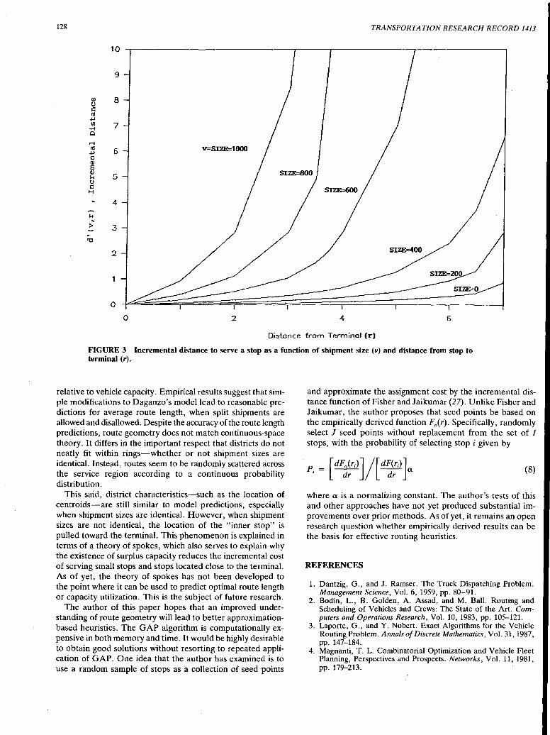
128 TRANSPORTATION RESEARCH RECORD 1413

10

9

Q) 8 CJ i:: Ctl .µ !I) 7 ·.-! 0

r-i Ctl 6 V=SIZE=1000 .µ i:: Q)

e Q)

5 1-1 CJ i:: H

4

1-1 .. > 3 -'tl

2

0 2 4 6

Distance from Terminal (r)

FIGURE 3 Incremental distance to serve a stop as a function of shipment size (v) and distance from stop to terminal (r).

relative to vehicle capacity. Empirical results suggest that sim­ple modifications to Daganzo's model lead to reasonable pre­dictions for average route length, when split shipments are allowed and disallowed. Despite the accuracy of the route length predictions, route geometry does not match continuous-space theory. It differs in the important respect that districts do not neatly fit within rings-whether or not shipment sizes are identical. Instead, routes seem to be randomly scattered across the service region according to a continuous probability distribution.

This said, district characteristics-such as the location of centroids-are still similar to model predictions, especially when shipment sizes are identical. However, when shipment sizes are not identical, the location of the "inner stop" is pulled toward the terminal. This phenomenon is explained in terms of a theory of spokes, which also serves to explain why the existence of surplus capacity reduces the incremental cost of serving small stops and stops located close to the terminal. As of yet, the theory of spokes has not been developed to the point where it can be used to predict optimal route length or capacity utilization. This is the subject of future research.

The author of this paper hopes that an improved under­standing of route geometry will lead to better approximation­based heuristics. The GAP algorithm is computationally ex­pensive in both memory and time. It would be highly desirable to obtain good solutions without resorting to repeated appli­cation of GAP. One idea that the author has examined is to use a random sample of stops as a collection of seed points

and approximate the assignment cost by the incremental dis­tance function of Fisher and Jaikumar (27). Unlike Fisher and J aikumar, the author proposes that seed points be based on the empirically derived function F0 (r). Specifically, randomly select J seed points without replacement from the set of I stops, with the probability of selecting stop i given by

P, = [ dFJ~r'V[ d~~,) }• (8)

where a is a normalizing constant. The author's tests of this and other approaches have not yet produced substantial im­provements over prior methods. As of yet, it remains an open research question whether empirically derived results can be the basis for effective routing heuristics.

REFERENCES

1. Dantzig, G., and J. Ramser. The Truck Dispatching Problem. Management Science, Vol. 6, 1959, pp. 80-91.

2. Bodin, L., B. Golden, A. Assad, and M. Ball. Routing and Scheduling of Vehicles and Crews: The State of the Art. Com­puters and Operations Research, Vol. 10, 1983, pp. 105-121.

3. Laporte, G., and Y. Nobert. Exact Algorithms for the Vehicle Routing Problem. Annals of Discrete Mathematics, Vol. 31, 1987, pp. 147-184.

4. Magnanti, T. L. Combinatorial Optimization and Vehicle Fleet Planning, Perspectives and Prospects. Networks, Vol. 11, 1981, pp. 179-213.

Hall

5. Vehicle Routing Methods and Studies (B. J. Golden and A. A. Assad, eds.), North-Holland Elsevier, Amsterdam, The Neth­erlands, 1988.

6. Daganzo, C. F. The Distance Traveled to Visit N Points with a Maximum of C Stops per Vehicle: An Analytical Model and an Application. Transportation Science, Vol. 18, 1984, p. 331-350.

7. Daganzo, C. F. The Length of Tours in Zones of Different Shapes. Transportation Research, Vol. 18B, 1984, pp. 135-146.

8. Newell, G. F., and C. F. Daganzo. Design of Multiple Vehicle Delivery Tours-I, a Ring Radial Network. Transportation Re­search, Vol. 20B, 1986, p. 345-364.

9. Beardwood J., J. H. Halton, and J.M. Hammersley. The Short­est Path Through Many Points. Proceedings of the Cambridge Philosophical Society, Vol. 55, 1959, pp. 299-327.

10. Few, L. The Shortest Path and the Shortest Road Through n Points. Mathematika, Vol. 2, 1955, pp. 141-144.

11. Stein, D. M. Asymptotic, Probabilistic Analysis of a Routing Problem. Mathematics of Operations Research, Vol. 3, 1978, pp. 89-101.

12. Verblunksy, S. On the Shortest Path Through a Number of Points. Proceedings of the American Mathematical Society, Vol. 2, 1951, pp. 904-913.

13. Christofides, N., and S. Eilon. Expected Distances in Distribu­tion Problems. Operational Research Quarterly, Vol. 20, 1969, pp. 437-443.

14. Haimovich, H., and A. H. G. Rinnooy Kan. Bounds and Heu­ristics for Capacitated Routing Problems. Mathematics of Op­erations Research, Vol. 10, 1985, pp. 527-542.

15. Haimovich, H., A. H. G. Rinnooy Kan, and L. Stougie. Analysis of Heuristics for Vehicle Routing Problems. In Vehicle Routing: Methods and Studies (B. L. Golden and A. -A. Assad, eds.), North-Holland, Amsterdam, The Netherlands, 1988, pp. 47-62.

16. Spaccamela, M., A. H. G. Rinnooy Kan, and L. Stougie. Hi­erarchical Vehicle Routing Problems. Networks, Vol. 14, 1984, pp. 571-586.

17. Daganzo, C. F., and R. W. Hall. A Routing Model for Pickups and Deliveries: No Capacity Restrictions on the Secondary Items. Transportation Science (in press).

129

18. Hall, R. W. Characteristics of Multi-stop/Multi-terminal Deliv­ery Routes, with Backhauls and Unique Items. Transportation Research, Vol. 25B, 1991, pp. 391-403.

19. Bertsimas, D. J., and G. van Ryzin. A Stochastic and Dynamic Vehicle Routing Problem in the Euclidean Plane. OR 210-90. Operations Research Center, Massachusetts Institute of Tech­nology, Cambridge, 1990.

20. Hall, R. W. Pickup and Delivery Strategies for Overnight Car­riers. Transportation Research (in press).

21. Simchi-Levi, D. Hierarchical Planning for Probabilistic Distri­bution Systems in Euclidean Spaces. Department of Industrial Engineering and Operations Research, Columbia University, New York, 1990.

22. Hall, R. W., Y. F. Du, and J. Lin. Integration of Discrete and Continuous Models for Routing Vehicles. Networks (in press).

23. Ong, H. L., M. J. Magazine, and T. S. Wee. Probabilistic Anal­ysis of Bin Packing Heuristics. Operations Research, Vol. 32, 1984, pp. 983-998.

24. Hall, R. W., and C. F. Daganzo. Vehicle Miles for. a Freight Carrier with Two Capacity Constraints. In Transportation Re­search Record 1038, TRB, National Research Council, Wash­ington, D.C., 1985, pp. 34-40.

25. Hall, R. W. Vehicle Packing. Transportation Research, Vol. 23B, 1989, pp. 103-121.

26. Dror, M., and P. Trudeau. Split Delivery Routing. Naval Re­search Logistics Quarterly, Vol. 37, 1990, pp. 383-402.

27. Fisher, M. L., and R. J aikumar. A Generalized Assignment Heu­ristic for Vehicle Routing. Networks, Vol. 11, 1981, pp. 109-124.

28. Little, J., K. Murty, D. Sweeney, and C. Karel. An Algorithm for the Traveling Salesman Problem. Operations Research, Vol. 11, 1963, pp. 972-989.

Publication of this paper sponsored by Committee on Transportation Supply Analysis.

130 TRANSPORTATION RESEARCH RECORD 1413

An IP-Norm Origin-Destination Estimation Method That Minimizes Site-Specific Data Requirements

Yuro CHAN AND M. YuNus RAHi

An efficient IP-approximation algorithm to estimate a likely ori­gin-destination (0-D) matrix while minimizing site-specific data­collection effort is presented. It was found that the trip-distribution curve is a useful supplement to site-specific link counts since it can be borrowed from a similar community, or that an outdated local curve can be employed without significant loss of accuracy. Imbedding such a generic trip-distribution curve within the al­gorithmic procedure gives a more accurate 0-D estimation and link-count reproduction in general, although the number of it­erations is increased. Test results from a medium-sized city sh9w that the extra computational effort is a small price to pay for the improvement in 0-D accuracy. The IP-approximation algorithm is shown to be theoretically related to familiar 0-D estimation techniques such as entropy maximization, information minimi­zation, and generalized inverse, yet it is more robust and theo­retically more satisfying.

The fundamental and indispensable data required to opera­tionalize origin-destination (0-D) estimation algorithms are link counts. Additional data requirements differ depending on the specific methodology. Some require an old 0-D matrix, often referred to as a base (or target) 0-D matrix, whereas others require a control total on productions and attractions, but they can be labeled as site-specific information. Consistent with the resource-saving objective of this class of 0-D esti­mation techniques, the intention here is to minimize the col­lection of site-specific data, and to the extent possible, use generic information transferable from other cities of similar size and urban structure (1). The authors propose to use trip­distribution curves, also known as trip-length frequency curves, to supplement basic site-specific data, such as link counts, given the invariant nature of these curves, which has been attributed to travel-time budget theories (2,3).

BASIC THEORIES

The 0-D estimation problem can be thought of as solving the linear equation set

AF =(af)F = V (1.1)

where A is an mxn' assignment matrix consisting of entries a7 (4,5). Let us say that the entry a7 assumes a value 1 for

Y. Chan, Department of Operational Sciences, Graduate School of E~gineering, Air Force Institute of Technology, Wright-Patterson Au Force Base, Ohio 45433. M. Y. Rabi, Associated Traffic Con­sultants, 99 S. Chester Avenue, Suite 200, Pasadena, Calif. 91106.

single-path assignment when an 0-D pair k uses a particular link i, and 0 otherwise. F is a variable vector of n' entries each of which is pk, where pk is the kth 0-D demand to b~ estimated. V is a vector of link counts, consisting of m ob­servations in the sample, each of which is V;, where V; is the ith link count. In the more general case of multipath assign­ment, af assumes a fractional value or 0. Thus for q-path traffic-assignment procedures, F will assume qn' = n entries, with each pk replicated q times for the q copies of the traffic assignment. Likewise, the A matrix is expanded tom by n in dimension, with each column replicated q times correspond­ing to the percentage of the 0-D demand that follows a par­ticular path.

Viewed in this light, the estimation of 0-D demands be­comes a matrix-inversion problem: F = A +y, where A+ is the generalized inverse of A. For an mxnA matrix (m < n) of rank m the generalized inverse A+ is simply A T(AA T)- 1, where both (V - AF)T(V - AF) and FTF are minimized. Here, the first dot-product is the deviation between observed and estimated link counts, following a typical least-square approach (6). The second is the sum of squares of P. For a fixed sum of P's (or F, the total number of trips in the study area), the minimization of FTF yields P = Fin' or an equal­ized set of 0-Ds, which does not necessarily minimize the first dot product.

It is interesting to note that the entropy-maximization for­mulation of the 0-D estimation problem (7), namely

F! max w = _n __ _ (1.2) fl (pk)! k=l

also yields the same solution for a given F. Both give rise to an equalized set of 0-D demands (8). This is an interesting finding inasmuch as the two approaches are among the most common methods of 0-D estimation.

Between the generalized-inverse and entropy-maximization formulations, there has been some debates as to the best way to estimate 0-Ds. Even though the matrix-inversion method appears simple, it was found through extensive experimen­tation that round-off errors during the computational process can be large ( 9 ,10). Moreover, generalized inversion some­times yields negative solutions, which have no physical inean­ing in the context of the problem discussed here ( 8). The entropy-maximization method, on the other hand, has the conceptual appeal of obtaining the most likely 0-D pattern, yet the process to operationalize Equation 1.2, and the results

Chan and Rahi

are far from perfect. For example, it has the tendency to "lock up" in the slightest presence of data inconsistency, which introduces infeasibility into the mathematical program. Chan et al. ( 4) and Xu and Chan (11,12) pointed out a more robust and more accurate algorithm for solving large scale 0-D es­timation problems. Maher (13) confirmed previous findings that both the maximum entropy model and its cousin, the information-minimization model, produce counterintuitive results. Hamerslag and Immers (14) pointed out some severe limitations of both entropy maximization and information minimization models. Yang et al. (15) showed that a con­strained least-square algorithm consistently yielded a more accurate and more reliable 0-D estimate.

In choosing among 0-D estimation methods, it is important to keep in mind the versatility consideration. For example, can the technique be easily applied to a number of cities with minimal data collection beyond link counts? In this context, universal parameters embedded in the algorithm that are transferable between cities are soug.ht. Extensive­experimentation with graph-theoretic parameters suggests that there are few commonalities among the network taxonomy (as represented in assignment matrices A) between cities (8). A linear network representing a transportation corridor, for example, appears to yield more consistent total number of trips for external-external, internal-external, and external­internal movements as compared with internal-internal move­ments. However, no satisfactory explanation can be found to account for this. As another example, eigenvalues of the as­signment matrix A have the strong appeal of characterizing the natural frequency of the network structure. However, when the matrix is not square in dimension, which is the rule rather than the exception, eigenvalues are often not available.

In view of travel-time budget theories, the authors identify the trip-distribution curve as one of the few transferable pa­rameters among cities of similar size and urban structure (2 ,3). If an 0-D estimation algorithm can take full advantage of this transferable parameter, it is a more serviceable technique inasmuch as it requires minimal site-specific data collection.

In reviewing Equations 1.1 and 1.2, one can see that there is no obvious relationship between the trip-distribution curve and generalized inverse of the assignment matrix because ma­trix inversion is simple an algebraic computational procedure. On the other hand, previous research by Chan et al. ( 4) in­dicates that there may be links between entropy maximization and trip-distribution curves. Trip-distribution curves-either borrowed or locally collected-can serve as another set of input data for this estimation approach. The payoff for imbed­ding the trip-distribution curve within entropy maximization appears high.

ENTROPY MAXIMIZATION APPROACH

If W is the entropy function as shown in Equation 1.2, it is typical to take its logarithm W' as a first step of maximization:

n

W' = log F! - L log P! (2.1) k=l

Using Stirling's approximation and after simplification, the

131

maximum entropy formulation can be expressed as

n

max Z = - L (P log P - P) (2.2) k=l

subject to the link counts V;:

n

L a7P = V; 'Vi (2.3) k=l

and the trip-frequence distributions Fe:

n

L p~pk = Pk(C)F = Fe 'V c (2.4) k=l

where

{1 If Fk is of duration C (C - AC s Cs C + AC)

p~ = 0 otherwise

(2.5)

Fe represents the total trips of duration C; and Pk( C) is the probability of a trip k being C min long.

In this light, (P~) = P can be thought of as a pxn matrix similar to the mxnA matrix, with p being the number of travel­cost intervals defined for the trip-distribution curve. To all these is added the nonnegativity constraint, P ::::: 0 'V k. Notice the given F in Equation 2.5 can either be supplied exogenously (collected locally) or generated endogenously (from local link counts and borrowed trip distribution). This will be discussed further when the algorithm is explained in detail.

The Lagrangian for this constrained optimizati<;m problem is

L ~ - X,, (F' log F' - F') - .t, A.(X,, af F' - v,) (2.6)

The symmetry between the second and third terms above clearly shows the suitability of trip-distribution data as sup­plement to link counts. A typical calculus solution to this Lagrangian yields.

exp(- L Ac) exp(- L A;) cEH iEK

(2.7)

where the summation is carried over all links i that carry flow between the 0-D pair k, denoted here as the set Kand all trip durations C that pertain to 0-D pair k, H.

Now setting

exp(-A;) V; 'Vi EK

V;

exp(-Ac) Uc 'V c EH (2.8)

Fe

132

results in

pk = (r1 v;V;) n ufc iEK cEH

(2.9)

Obviously, in the case of all-or-nothing single-path assign­ment, the set H has a membership of one. This method of estimating 0-D demands yields the conventional multipro­portional product-form solution, except that the explanatory variables include trip-frequency parameters-specifically the Lagrange multiplier Ac defined for each trip duration C.

To arrive at a satisfactory solution to Fk is no easy task, as many researchers have labored continuously during the last 2 decades on this problem. First, the objective function of the mathematical program as formulated in Equations 2.1-2.5 is nonlinear, and it is not strictly concave in P. Therefore, it does not necessarily have a unique solution in terms of the 0-D variables P's (16). Besides, multiple optima in terms of nonunique 0-D specific link volumes and path routings exist. This nonuniqueness is well known among researchers because the underlying problem, that of finding an 0-D matrix that produces the observed link flows and trip distribution, is un­derspecified. In other words, numerous 0-D matrices can produce a given set of observed link counts and a specified trip-distribution curve. The choice between these alternative matrices has to be based on additional criteria. Finally, nu­merical intricacies are involved in solving a nonlinear pro­gramming problem as formulated by Equations 2.1-2.5. Most hill-climbing algorithms are sensitive to the redundancies and inconsistencies within and between constraints shown in Equations 2.3 and 2.4. (14).

MATHEMATICAL PROGRAM BASED ON Ip-APPROXIMATION

To overcome the shortcomings of traditional approaches such as entropy-maximization, the comprehensive set of criteria that the estimated 0-D solution is to satisfy, including the additional criteria that may guarantee convergence and so­lution uniqueness, are reviewed. The authors have already mentioned that the 0-D estimation problem has to minimize the deviations between the observed link volumes and the estimated values. This can be related to the IP-approximation methods (p = 1, 2, ... oo), in which deviations (between observed and estimated values) are minimized according to some predefined representation of norm vectors. Ip-norms represent one of the most general ways to measure deviation of the estimates from the observed values. For example, the / 1-approximation will minimize the sum of the absolute de­viations (16,17):

I,: minllV - AFll, = min,~ Iv, - kt, a~F'I (3.1)

The /2-approximation, on the other hand, minimizes the ab­solute value of the sum of the squares of the deviation (i.e., the traditional least square solution):

12: minllV - AFllz

[

m ( n )2]112 = min ~ V; - L af P

1=1 k=l (3.2)

TRANSPORTATION RESEARCH RECORD 1413

Finally, the loo-approximation, also known as the Chebyshev approximation, minimizes the maximum of the absolute de­viations (18):

Any one of the IP-norms may be viewed as an objective func­tion. By setting the maximum allowable deviation for link­volume replication, bounds are placed on the accuracy of the estimation-a desirable feature of a solution algorithm of this kind.

A Chebyshev approximation similar to Equation 3.3 may be written for trip-distribution replication:

/~: minllFc - PFlloo = min max I Fe - i P~PI (3.4) l:Sc:sp k = 1

The same applies to 11 and 12 norms as well. The properties of Chebyshev approximation, are demonstrated in the fol­lowing simple nonnetwork case:

/':,: min maxlP - F~I

n'

s.t. 2: P = F k=l

Vk (3.5)

All F~s are further assumed to be equal. It can be shown quite easily that the solution is P = Fin' (i.e., all estimates are equalized as observed in both the entropy model and the generalized inverse model). It can be seen, therefore, that the loo-approximation plays a similar role as entropy and in­verse models, but it does much more. Suppose f!s are not equal. The estimates P = F~ as long as "i,kF~ = F.

On the other hand, if "i,kF~ -=#= F

p =IF~ - ~Fl (3.6)

where ~F = (lln')IF0 Fl." It can be seen, therefore, that the loo-approximation tracks the observed 0-D values instead of simply equalizing the grand sum F, which is a highly de­sirable property.

At this point, it appears desirable to use Equation 3.5 as a criterion for measuring the performance of the model. How­ever, the base 0-D's F\s are often not available. Even if they are, it is not clear whether the base 0-D should be mimicked. For these reasons, it is not an operational objective function. A more practicable approach is to look at link and trip­distribution reproduction. Thus with Equations 3.3 and 3.4 as the major solution criteria, an optimization model can be set up with this additional constraint beyond Equations 2.3 and 2.4 if desired:

n

LIP - F~I ~ x (3.7) k=l

This constraint ensures that the estimated 0-Ds are not very different from the base 0-Ds, F~. Specifically, one limits the

Chan and Rahi

·maximum total deviation to be X. Similarly, a second con­straint can be set .up to limit the deviation between the user­optimizing link travel-cost at V; and the estimated total travel costs to Y.

(3.8)

Notice that in this constraint, C;(x) stands for the link travel­cost function and Ck stands for the estimated multipath travel­cost between the 0-D pair k (19). In order to operationalize this constraint, link counts will have to be collected for the entire network on all m links.

Constraint Equation 3.7 may or may not be effective de­pending on whether a base 0-D trip demand matrix is avail­able. Equation 3.8, while more readily enforceable and well correlated to 0-D reproduction (4), is often too aggregate a measure of solution accuracy in the judgment of the authors, since many different 0-D matrices can give rise to the same deviation Y. For all practical purposes, link count reproduc­tion accuracy (or!,,, in Equation 3.3) and trip-frequency rep­lication (Equation 3.4) are the only tangible measures of al­gorithmic convergence.

A new mathematical program is proposed with the objec­tive functions 3.3 and 3.4. The program's first order condi­tions-which require (among others, such as Equations 3.7

· and 3.8) that the link counts and trip-distribution curves be reproduced-are to be met within some convergence toler­ance, rather than exactly. Thus, Equations 2.3 and 2.4 in the entropy maximization formulation effectively turned into ob­jective functions. Furthermore, an iterative descent-gradient method is proposed for the solution of these objective func­tions-rather than an ascent method for 2.1.

To show how the solution to the surrogate mathematical program actually yields a solution to the original 0-D esti­mation problem is no easy task. For that matter, researchers have been struggling with this problem, including those who work with the traditional entropy approach. Many of the ar­guments would have to be less than rigorous. First, to the extent that some of the widely disseminated formulations such as matrix inversion yields a least square solution (V - AF)T(V - AF), objective function 3.2 and its gener­alization 3.3 are plausible surrogates, following the arguments made in Equations 3.5 and 3.6. It is a simple extension to cover the minimization of (Fe - PF)T(Fc - PF) as well. If desirable, one can view this as a disaggregation of the entropy objective function shown as Equation 2.6, wherein the second and third terms are taken as the two objective functions to be minimized; the first term may be taken care of implicitly by constraint 3. 7 and the general properties of l°"-norm as shown in Equation 3.5.

Second, the multiproportional product solution of Equation 2. 7 strongly suggests gradient algorithms, in which the Lan­guage multipliers Ai and Ac serve as weights placed on the relative importance of link count reproduction or trip fre­quency reproduction during optimization in Equation 2.6. Lagrange multipliers are interpreted in this case as the extent to which Equations 23 and 2.4 are satisfied, just as the mul­tiobjective optimization algorithm involving Equations 3.3 and 3.4 tries to trace the noninferior solutions.

In summary, the mathematical program proposed to solve includes Equations 3.3, 3.4 and 1.1 of the original problem.

133

To the extent that the entropy-maximization and matrix­inversion paradigm is a widely disseminated description of the original 0-D estimation problem, the authors have tried to show the relationship between their formulation, the matrix inversion, and the entropy formulations. No attempt has been made to show that the formulation will yield a solution such as Equation 2.9 which by itself is an approximation. The authors' approach is much more fundamental, in that the original 0-D estimation problem is stated in terms of lP­approximation, where the quantifiables such as link counts and frequency distributions are to be replicated. After some lengthy discussion, the authors finally recommended p = oo,

which echoes the intuitive requirement to minimize the worst deviations from the observed and the most likely estimate interpretation of entropy models, subject to the network ge­ometry constraint on flow (Equation 1.1). In the following section, it will be shown that aside from a regular multi­objective linear programming package, a more efficient gra­dient algorithm can be readily put forth to solve this minimax programming problem consisting of two objective functions (3.3 and 3.4) and a linear constraint (1.1). Also the optimi­zation criteria in the algorithm are equivalent to and more encompassing than the generalized inversion and entropy approaches.

ALGORITHM

Learning from the computational experiences of existing so­lution algorithms (4,11,12,14,20-22), the following iterative gradient algorithm is suggested for the loo-norm minimization model:

Initialization

The iterative algorithm can be started by setting the iteration counters to zero (s = 0). Then the following is defined.

P(O) = F~ (4.1)

where the base 0-Ds (such as an old 0-D matrix) are avail­able. Alternatively,

P(O)

m

"' a~P L.J ' ' i=l m

2: af i=l

(4.2)

for the situation where link counts are the only information available. Here Ff = VJ ~k'= 1 af Vi E K. Finally,

m m

L a~P ' ' L af PWi

Fk(Q) i=l i=l (4.3) m m

2: af 2: af i=l i=l

where the trip-distribution curve Fe is available in addition to link counts. In Equation 4.3, Pf = af Pk(C)/2.,'k= 1

af Pk(C), and Pk(C) stands for the probability that trip k has the same travel cost C as read from the trip-frequency dis-

134

tribution Fe Extensive computations by Chan et al. ( 4) and Xu and Chan (11,12) show that of all three initialization pro­cedures, the last one (Equation 4.3) is the most effective.

This result is not surprising since Equation 4.2 is nothing more than the inverse of· a regular assignment according to Equation 1.1. Its fundamental structure is related to entropy maximization, which yields P = Fin' when af = 1 for all i and k. In other words, imagine a network in which sampled links carry flows from every 0-D pair, then Equation 4.2 reduces to P = Fln 1

• This applies, for example, to F traffic counts on a freeway section, from which the pertinent en­trance and exit ramps of the traffic are to be inferred. The result is an equal amount of traffic for each entrance and exit ramps. Another way of saying this is that when network ge­ometry is totally set aside, equal 0-Ds would be the most likely inference from entropy maximization. When network geometry is taken into account, Equation 4.2 will result.

In Equation 4.3, 0-D inference is assisted by the knowledge of the trip-distribution curve. Thus, not only does network information get used, but trip-distribution information is taken into account as well. To see this more clearly, consider the close cousin of entropy maximization: the information mini­mizing model ( 14):

(4.4)

such that

(4.5)

where bj can assume the form of af or P~, and di can assume the form of V; or Fe, as shown in Equations 2.3 and 2.4. (Setting P = 1 for all k, or when there is no prior information, results in the familiar entropy maximization model.)

Solution of this model yields

(4.6)

where_R0 = exp( -1) and

(4.7)

where

(4.8)

Notice this is the same as Equation 2. 7 in the case of single­path assignment, except for the sign which simply reflects the difference between information minimization and entropy maximization. Most important, rearranging the multiproduct form of Equation 4.6 into P = F!RoRcR; shows that just like a base 0-D matrix F! (Equation 4.1), Re is simply another piece of prior information that can assist in more accurate determination of P. Although links between models are established, this formulation further accentuates some of the shortcomings of information/entropy formulations. First, Equation 4.5 is not defined for F! = 0. Second, incon­sistencies in specifying Equation 4.5 will "derail" any solution

TRANSPORTATION RESEARCH RECORD 1413

algorithms for the nonlinear program, as mentioned previ­ously. This will be demonstrated in an example. The /00-

approximation algorithm advanced here is rid of these problems.

lte~ation

After initialization, algorithmic steps can be written for the remaining iterations of the algorithm. In the following steps, the iteration index s is set to one to start the gradient algorithm.

Step 1. The various link volume estimates V;(s) are deter­mined from a traffic assignment in accordance with Equation 2.3 (or 1.1 of the original formulation):

n

L af P(s) = V;(s) i = 1, 2, ... , m k=1

Step 2. Modify trip-probability Equation 2.4 to compute the total number of trips of duration C, Fc(s), from a given trip distribution:

n

2: P~P(s) = Pk(C)F(s) = Fc(s) c = 1, 2, ... 'p k=1

where F(s) is the sum of estimated trips during the current sth iteration, and Fc{s) is the sum of all P(s) that belong to interval c. Instead of an extogenously determined Fin Equa­tions 1.2 and 3.5, this algorithm has the option to make F self-adjusting. The result is that P has as much a tendency to "track" the F! as to equalize among themselves.

Step 3. The link volume estimates V;(s) are compared with the observed volumes in the form of an error ratio:

Rk( ) - _!j__ k ; s - V;(s) a; i = 1, 2, ... , m

Likewise, for the trip distribution Fc{s).

k()-~Pk RC s - Fc(s) c c = 1, 2, ... 'p

(4.9)

(4.10)

A single composite error ratio can be obtained for all links carrying flows between 0-D pair kif desired:

[ ~ afRf(s) + ~ ~R~(s)]

(~a7+p~) Vk (4.11)

Step 4. The composite error ratio is then used as an ad­justment factor to the pertinent 0-D estimate F/ from the previous iteration:

vi, k (4.12)

where th~ iteration index s is now incremented by 1. These four steps are applied to all links with an observed ·

flow and repeated successively for convergence. The iterative steps yield a new set of estimates each tim~e not only for the

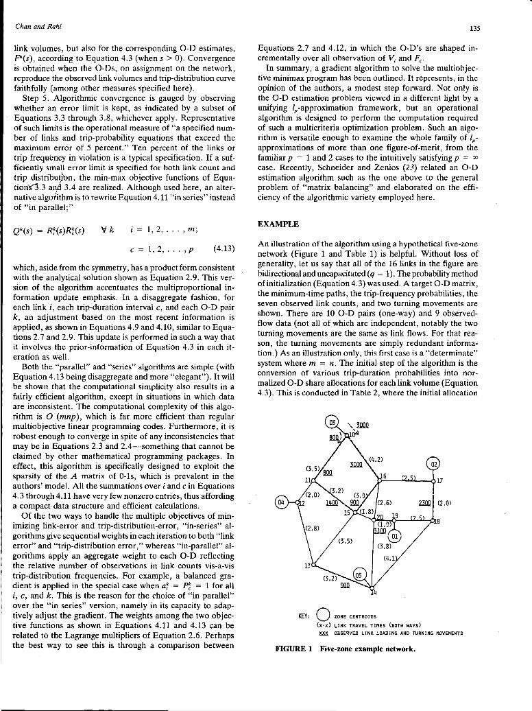
Chan and Rahi

link volumes, but also for the corresponding 0-D estimates, P(s), according to Equation 4.3 (whens> 0). Convergence is obtained when the 0-Ds, on assignment on the network, reproduce the observed link volumes and trip-distribution curve faithfully (among other measures specified here).

Step 5. Algorithmic convergence is gauged by observing whether an error limit is kept, as indicated by a subset of Equations 3.3 through 3.8, whichever apply. Representative of such limits is the operational measure of "a specified num­ber of links and trip-probability equations that exceed the maximum error of 5 percent." Ten percent of the links or trip frequency in violation is a typical specification. If a suf­ficiently small error limit is specified for both link count and trip distribXit\:m, the min-max objective functions of Equa­tion'S3.3 a 3.4 are realized. Although used here, an alter­native algo ithm is to rewrite Equation 4.11 "in series" instead of "in parallel~"

Qk(s) = R7(s)R~(s) 'V k i = 1, 2, ... , m;

c = 1, 2, ... 'p (4.13)

which, aside from the symmetry, has a product form consistent with the analytical solution shown as Equation 2.9. This ver­sion of the algorithm accentuates the multiproportional in­formation update emphasis. In a disaggregate fashion, for each link i, each trip-duration interval c, and each 0-D pair k, an adjustment based on the most recent information is applied, as shown in Equations 4.9 and 4.10, similar to Equa­tions 2.7 and 2.9. This update is performed in such a way that it involves the prior-information of Equation 4.3 in each it­eration as well.

Both the "parallel" and "series" algorithms are simple (with Equation 4.13 being disaggregate and more "elegant"). It will be shown that the computational simplicity also results in a fairly efficient algorithm, except in situations in which data are inconsistent. The computational complexity of this algo­rithm is 0 (mnp), which is far more efficient than regular multiobjective linear programming codes. Furthermore, it is robust enough to converge in spite of any inconsistencies that may be in Equations 2.3 and 2.4-something that cannot be claimed by other mathematical programming packages. In effect, this algorithm is specifically designed to exploit the sparsity of the A matrix of 0-ls, which is prevalent in the authors' model. All the summations over i and c in Equations 4.3 through 4.11 have very few nonzero entries, thus affording a compact data structure and efficient calculations.

Of the two ways to handle the multiple objectives of min­imizing link-error and trip-distribution-error, "in-series" al­gorithms give sequential weights in each iteration to both "link error" and "trip-distribution error," whereas "in-parallel" al­gorithms apply an aggregate weight to each 0-D reflecting the relative number of observations in link counts vis-a-vis trip-distribution frequencies. For example, a balanced gra­dient is applied in the special case when a7 = P~ = 1 for all i, c, and k. This is the reason for the choice of "in parallel" over the "in series" version, namely in its capacity to adap­tively adjust the gradient. The weights among the two objec­tive functions as shown in Equations 4.11 and 4.13 can be related to the Lagrange multipliers of Equation 2.6. Perhaps the best way to see this is through a comparison between

135

Equations 2.7 and 4.12, in which the 0-D's are shaped in­crementally over all observation of V; and Fc-

In summary, a gradient algorithm to solve the multiobjec­tive minimax program has been outlined. It represents, in the opinion of the authors, a modest step forward. Not only is the 0-D estimation problem viewed in a different light by a unifying IP-approximation framework, but an operational algorithm is designed to perform the computation required of such a multicriteria optimization problem. Such an algo­rithm is versatile enough to examine the whole family of /P­approximations of more than one figure-of-merit, from the familiar p = 1 and 2 cases to the intuitively satisfying p = oo

case. Recently, Schneider and Zenios (23) related an 0-D estimation algorithm such as the one above to the general problem of "matrix balancing" and elaborated on the effi­ciency of the algorithmic variety employed here.

EXAMPLE

An illustration of the algorithm using a hypothetical five-zone network (Figure 1 and Table 1) is helpful. Without loss of generality, let us say that all of the 16 links in the figure are bidirectional and uncapacitated ( q = 1). The probability method of initialization (Equation 4.3) was used. A target 0-D matrix, the minimum-time paths, the trip-frequency probabilities, the seven observed link counts, and two turning movements are shown. There are 10 0-D pairs (one-way) and 9 observed­flow data (not all of which are independent, notably the two turning movements are the same as link flows. For that rea­son, the turning movements are simply redundant informa­tion.) As an illustration only, this first case is a "determinate" system where m = n. The initial step of the algorithm is the conversion of various trip-duration probabilities into nor­malized 0-D share allocations for each link volume (Equation 4.3). This is conducted in Table 2, where the initial allocation

KEY: 0 ZONE CENTROIDS

<x·x> LINK TRAVEL TIMES (BOTH WAYS)

~ OBSERVED LINK LOADING AND TURNING MOVEMENTS

FIGURE 1 Five-zone example network.

I

136

TABLE 1 Data for Five-Zone Network

Zone Pair k

1 2 3

4 5 6

7 8 9 10

0-D Zones*

1 - 2 1 - 3 1 - 4

1 - 5 2-3 2-4

2-5 3 - 4 3 - 5 4-5

0-D Path k

19,18,17 19,20,16,10 19,20,15,11, 12 19,20,14 17,16,10 17,16,15,11, 12 17,18,14 10, 11, 12 10, 16,20, 14 12, 13, 14

Skim Tree C'

5 8 8

5 7 11

6 6 11 6

TRANSPORTATION RESEARCH RECORD 1413

Trip Freq. P%

27 15 15

27 15 14

29 29 14 29

Target 0-D,P

1,100 1,000 500

1,600 1,500 900

1,200 800 500 900

Final Est. 0-D, P(7)

1,139 848 653

1,575 1,488 804

1, 179 806 674 907

* A symmetric 0-D matrix is assumed. Thus an 0-D pair p-q (p <q) stands for both zone pairs p-q and q-p.

of link volumes is made to arrive at Ff. Notice that there is more than one estimate of each 0-D volume, as pointed out earlier in the description of the algorithm. According to Equa­tion 4.3, these different estimates from the different link vol­umes are averaged, yielding P(O)'. The algorithm proceeds to the iteration phase .in which the five-step procedure is ex­ecuted. Such a procedure is shown in Table 3, where the

TABLE 2 /"'-Norm Algorithm

Link Obs. Zonal Trip Vol. Avg. Link in Vol. Pair Freq. Normal Alloc. 0-D

Fig. 1° V; k pk% P;k % F80) f'<(O)

10-11· 800 8(3-4) 29 100.0 800 800

2 10-16b 3000 2(1-3) 15 34.1 1023 919 5(2-3) 15 34.1 1023 1023 9(3-5) 14 31.8 954 954

3 11-15 1400 3(1-4) 15 51.7 724 770 6(2-4) 14 48.3 676 788

4 13-14 900 10(4-5) 29 100.0 900 900

5 15-16 900 6(2-4) 14 100.0 900 788

6 17-18 2300 1(1-2) 27 48.2 1109 1109 7(2-5) 29 51.8 1191 1191

7 19-20 3100 2(1-3) 15 26.3 816 919 3(1-4) 15 26.3 816 770 4(1-5) 27 47.4 1469 1469

9923 • same as turning movement from 3-10 to 10-11 b same as turning movement from 3-10 to 10-16 0 Link (i,j), where i <j, is bi-directional. It stands for both (i,j) and G ,i).

allocated link volumes P(s) are revised according to both the link-error ratio (Equation 4.9) and the trip-distribution error ratio (Equation 4.10). The adjustment using the error ratios results in a revised set of 0-D allocations from link counts, hence revised average 0-D estimates P(s), in each iteration. When the 5 percent error/10 percent violation convergence criteria are met (Step 5 of the algorithm), the average 0-D

Iteration One Iteration Two Est. Trips Adj. Adj. Avg. Adj. Adj. Avg. of Dur. ratio ratio est. ratio ratio est. C, F 0 (0) R81) Rck(l) F;k(l) FcO) R8.2) R/(2) F;"(2)

2876 1.000 0.995 798 2880 1.002 0.999 799

1488 1.036 0.881 869 1490 0.994 0.929 849 1488 1.455 1274 1490 1.170 1378 1389 0.797 874 q90 0.874 817

1488 0.899 0.881 701 1490 0.988 0.949 684 1388 0.797 716 1390 0.874 715

2876 1.000 0.995 898 2880 1.002 0.999 898

1388 1.142 0.797 716 1390 1.256 0.874 715

2678 1.000 1.039 1130 2682 0.992 1.026 1140 2876 0.995 1188 2880 0.999 1183

1488 0.982 0.881 869 1490 1.015 0.949 849 1488 0.881 701 1490 0.949 684 2678 1.039 1484 2682 1.026 1515

9932 9978

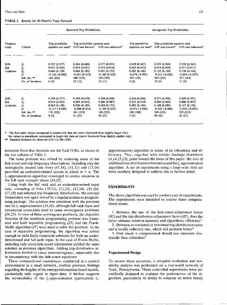
Chan and Rahi 137

TABLE 3 Results for 42-District York Network

Borrowed Trip Probabilities Site-specific Trip Probabilities

Violation Trip-probability Trip-probability equation used Trip-probability Trip-probability equation used Limit Criteria equation not used* 0-D sum known* 0-D sum unknown* equation not used* 0-D sum known* 0-D sum unknown*

20% Z1 0. 707 (0.577) 0.661 (0.668) 0.577 (0.671) 0.629 (0.607) 0.555 (0.560) 0.539 (0.543) link Zi 0.027 (0.026) 0.011 (0.021) 0.019 (0.018) 0.023 (0.032) O.Ql8 (0.018) 0.017 (0.017) violations 2, 0.066 (0.128) 0.004 (0.182) 0.091 (0.175) 0.092 (O. I06) 0.122 (O.I09) 0.139 (0.134)

D -0.123 (-0.040) -0.021 (0.019) -O. I09 (0.028) -O.Q78 (-0.091) -0.013 (-0.026) -0.034 (-0.057) Std. dev.** 166 (222) 188 (316) 168 (320) 185 (192) 243 (223) 237 (214) No. of iterations 6 (3) 33 (12) IO (11) 5 (3) IO (9) 11 (9)

IO% Z1 0. 708 (0.577) 0.658 (0.678) 0.584 (0.690) 0.630 (0.606) 0.573 (0.590) 0.549 (0.551) link Zi 0.019 (0.026) 0.005 (0.015) 0.006 (0.007) 0.015 (0.018) 0.004 (0.005) 0.006 (0.007) violations 2, 0.065 (0.128) 0.020 (0.189) 0.084 (0.173) 0.092 (0. I04) 0. I08 (0.089) 0.137 (0.130)

D -0.117 (-0.040) -0.008 (0.014) -O. I09 (0.033) -0.072 (-0.085) -0.035 (-0.008) -0.036 (-0.053) Std. dev.** 170 (222) 191 (315) 168 (322) 190 (199) 243 (223) 235 (215) No. of iterations 8 (3) 51 (27) 38 (27) 7 (5) 49 (41) 56 (27)

* The first entry values correspond to smaller-city data set (curve borrowed from slightly larger city); the values in parentheses correspond to larger-city data set (curve borrowed from slightly smaller city).

** Standard deviation for observed 0-D's is 284 (305).

estimates from that iteration are the final 0-Ds, as shown in the last column of Table 1.

The same problem was solved by removing some of the link count and trip-frequency observations. Including only the strategically located link flows (17,18), (11,12) and (13,14) provided an underdetermined system in which m < n. The /"'-approximation algorithm converged to similar solutions as the full rank example above (24,25).

Using both the full rank and an underdetermined input data, consisting of links (10,11), (11,15), (13,14), (15,16), (17 ,18) and selected trip-frequency distributions, the entropy formulation was again solved by a regular nonlinear program­ming package. The solution was consistent with the previous one by /00-approximation (24,26), although full-rank input and extraneous constraints tend to cause convergence problems (24,25). In view of these convergence problems, the objective function of the nonlinear programming problem was linear­ized and both separable programming (25) and the Frank­Wolfe algorithm (27) were used to solve the problem. In the. case of separable programming, the algorithm was robust enough to yield fairly consistent solutions for both an under­determined and full-rank input. In the case of Frank-Wolfe, including only seven link-count information yielded the same solution as previous algorithms. Adding trip-distribution in­formation tended to cause nonconvergence, apparently due to inconsistency with the link-count equations.

These computational experiences, conducted in a control environment in a small network, confirm previous findings regarding the fragility of the entropy/information-based models, particularly with regard to input data. It further supports the serviceability of the IP-approximation (particularly la,,-

approximation) algorithm in terms of its robustness and ef­ficiency. This, together with similar findings elsewhere (4,14,15,23), point toward the focus of this paper: the role of additional trip-distribution information and the IP -approximation algorithm. A set of experiments using a large-scale data set were carefully designed to address this in further detail.

EXPERIMENTS

The above algorithm was used to conduct a set of experiments. The experiments were intended to resolve three computa­tional issues:

1. Between the use of the link-count-adjustment factor (Rf) and the trip-distribution-adjustment factor (R~), does the latter enhance solution accuracy and algorithmic efficiency?

2. Between an outdated or borrowed trip distribution curve and a locally collected one, which will perform better?

3. How much is compromised should one minimize site­specific data collection?

Experimental Design

To answer these questions, a complete evaluation and sen­sitivity analysis was performed on a real-world network of Xork, Pennsylvania. These controlled experiments were sci­entifically designed to evaluate the performance of the al­gorithm, particularly its ability to compute an entire family

I 138

of IP-norms over several criteria. One of the evaluation mea­sures is the normalized deviation between the observed and estimated 0-Ds following the constraint defined in Equation 3.7, where the observed 0-Ds are available (since it is a controlled experiment):

n

L IP - F!I k=l (5.1)

Another evaluation measure is the normalized deviation between estimated and observed link volumes, following the objective function defined in Equation 3.1:

m (5.2) L V; i=l

Although not used here, a similar criterion can be defined for the compliance with a local trip-distribution function (but not necessarily with a borrowed curve).

A third measure, related to Equation 3.8, documents the difference between the observed versus estimated total costs (in vehicle-hours of travel). The following is a special single­path case of constraint 3. 8 when af assumes 0-1 values (instead of fractional values).

m n

L c;V; - L CkP i=l k=l (5.3)

The controlled nature of the experiment allows Z3 to be computed even though not all link counts are used for 0-D estimation.

The fourth is a measure of the difference between sums of the estimated 0-Ds and the observed 0-Ds. This allows one to assess whether the algorithm overestimates or underesti­mates the total number of 0-Ds:

n n

L pk - L F! D k=l k=l (5.4) n

L F! k=l

The spread of the estimated 0-Ds is compared with the observed via the standard deviation (CJ) statistic. This allows one to gauge the uniformity of the 0-D estimates inasmuch as both the generalized-inverse and entropy-maximization procedures tend to equalize £k's. A small value of CJ, for example, shows uniformity among 0-D estimates for the /P­approximation algorithm and vice versa.

Finally, all experiments are eval~ated by the rate of con­vergence, defined as the number of iterations required to reach a specific error limit. An example of such a limit is the percentage of links that are outside the error tolerable for link volume estimates. We will recall that this termination criterion realizes the /""-approximation as shown in Equations

TRANSPORTATION RESEARCH RECORD 1413

3.3 and 3.4-particularly the two first order conditions of this gradient algorithm.

As mentioned previously, each experiment is designed to compare the proposed algorithm with the version where the trip-probability equation is not used. When the trip­probability equations are used, two cases need to be tested: either the sum of the 0-Ds is known or that it is not. In the former case, the equalizing property, as shown in Equation 3.5, is tested. In t~e latter case, the absence of such property is expected-all through the use of the standard deviation (CJ) statistic. In the case of a site-specific trip-distribution curve being available, it is more likely than not that the 0-D sum is also available. On the other hand, when a borrowed trip distribution curve is used, it is unlikely that such a sum is known.

The above experimental design is best illustrated by the five-zone example, where a locally collected trip-distribution curve is assumed available. To make the example interesting, it is assumed also that the total number of trips is not known a priori. The algorithm is iterated until no more than 10 per­cent of the link volumes and trip-probability equations exceed the 5 percent error. The thrust of comprehensive tests were performed in the York network, which consists of 42 districts, 101 nodes, and 861 symmetrical 0-D pairs-a considerably large network for such experimentation. Although the vio­lation limit is 10 percent for the five-zone example, both 10 percent and 20 percent are tested for the 42-district network.

To support the theme of the research, the authors exper­imented with trip-distribution transferability. Two curves are identified in York, the first representing an outdated distri­bution, the second, the current distribution:

15.82 C exp( -0.379C) R2 = 0.975 (5.5)

12.85 C exp(-0.353C) R2 = 0.927 (5.6)

Since the York metropolitan area has grown in population and development during the last 2 decades, the authors refer to the outdated curve as from the "smaller city data set," whereas the current curve is from the "larger city data set." Experiments were then performed on the current data set consisting of network geometry, base matrix, and sample counts using an outdated trip-distribution curve. Conversely, exper­iments were performed on the outdated data set (or smaller­city data), borrowing the current trip-distribution curve. Al­though the former set of experiments represents the common practice, the latter is also valid from an experimental design standpoint, in that both cases represent borrowing a distri­bution curve from a "similar" city.

Notice a trip-distribution curve is involved in the initiali­zation phase (Equation 4.3), even though it may not be in­cluded in the iterative phase. For this reason, there are two columns again under the heading "trip probability equation not used" in Table 3, corresponding to the smaller-city and larger-,city curve, respectively, being used to initialize the algorithm.

Empirical Results

Notice in Table 3 that the proposed algorithm consistently gives an equally accurate and often a more accurate 0-D and

Chan and Rahi

link-count reproduction (Z1 and Z2 ) when the 0-D sum is not known a priori. This is gratifying in that the objective of minimizing site-specific data requirement is achieved, where the additional local information on the total-number-of-trips is not necessary to obtain quality algorithmic performance. Not only is the information superfluous, but its absence gives rise to more accurate 0-D estimation than when it is collected. Instead of merely equalizing the estimated values (as in the

. case of matrix inversion and entropy maximization), the es­timated 0-Ds are now allowed to approximate the variability of the target 0-Ds better.

Along this line, the results from experiments where a bor­rowed curve is used (Table 3) are comparable in accuracy to those where a curve is available locally. As long as a trip­distribution curve is employed, a 33 percent link-sampling rate as used in the experiments in Table 3 does not significantly compromise the 0-D estimation accuracies when compared with the 100 percent sample. The 100 percent sample is not included here due to space limitations. The interested reader may consult work by Rahi (8) for this information. As it turns out, the algorithm becomes more efficient and converges faster with the 33 percent sampling rate because there are fewer inconsistencies to resolve. This finding reinforces the com­puter runs on the five-zone example and further supports the authors' claim that although the algorithm is robust enough to handle redundant data, it is much less data-hungry for the same degree of accuracy.

As suggested previously there is little advantage, if any, to gathering site-specific data, such as the total number of 0-D trips. First, it introduces inaccuracy to the solution by equal­izing 0-Ds, as mentioned previously. Also, it tends to prolong the number of iterations before convergence is obtained in all cases. This is again a gratifying finding, saying that col­lecting irrelevant data does not only waste resources, it also harms the technical performance of the algorithm.

Because the 0-D estimates are required to conform to a prescribed trip distribution, more prior information is im­posed on the estimation process than other traditional algo­rithms and hence results in more heterogeneous 0-D esti­mates that better approximate the base 0-Ds. This is illustrated by Equation 4.3 and most particularly by Equation 4.5. The authors' claim, however, is highly predicated upon the shape of the trip-distribution curve. For example, a more peaked distribution curve from a smaller city tends to result in a much less uniform set of 0-Ds (Equations 5.5 and 5.6, and Table 3). A more peaked curve also tends to result in a large 0-D sum in general.

One point about the use of trip-distribution curves is quite clear. Should it be employed in 0-D estimation, an accurate specification of the probability values is advisable for better overall algorithmic performance. This is true for all cases­whether the trip-distribution curve is borrowed, and irre­spective of the violation limit set in the convergence criteria. Numerical round-odd errors in trip-distribution input tend to prolong algorithmic convergence because there are more in­consistencies to reconcile.

For the same reason, including trip-probability constraints typically prolongs the number of iterations required when compared with using link counts alone. It was found that the lower the error limit set, or the minimax objective functions are to be better achieved, the larger the number of iterations required to resolve these inconsistencies-as one would ex-

139

pect. For example, lowering from a 20 percent link violation rate to 10 percent dramatically increases the number of it­erations by a factor of five. This is the price one pays for saving site-specific data-collection efforts. Irrespective of the increase, computation time is no more than a few minutes on an Amdahl V-816 because the computational complexity of such an algorithm is polynomial.

SUMMARY AND CONCLUSION

On the basis of the plethora of research on origin-destination estimation during the last 2 decades, the authors synthesize here an improved theory and algorithm that is a general ver­sion of entropy maximization, information minimization and matrix-inverse models. The objective is to estimate 0-Ds with the least amount of site-specific data collection. Beyond the site-specific link counts, the authors wish to rely exclusively on generic data (i.e., data that can be borrowed from other communities of similar size and development structure or from data collected for the same community in a previous survey). Specifically, the trip-frequency or trip-length distribution curve is identified as the most promising piece of "transferable" information to supplement site-specific link counts.

An /00-approximation algorithm is synthesized on the basis of experiences with the widely disseminated generalized­inversion and entropy-maximization theories. The authors' approach takes advantage of their strengths, such as the an­alytical property of entropy-maximization, which readily al­lows for the inclusion of generic information such as trip­frequency curves in a multiproduct form. IP-approximation methods p = 1, 2, ... , oo represent a more fundamental approach to modeling the original 0-D estimation problem than the least-square assumption (p = 2) of generalized in­verse. The result is a flexible, successive-approximation al- . gorithm, assuming the multiproportional product form. In this multiobjective optimization model, adjustments to 0-D es­timates are made not only through link-count reproduction, but also trip-frequency reproduction. The latter represents the unique feature of the algorithm presented in this paper.

Care was exercised in the design of experiments, where the algorithm was compared with a version in which the trip­frequency information was not fully used. On the basis of testing of the 42-district York, Pennsylvania, network, it was found that the algorithm generally gives more accurate 0-D and link-count reproductions. Furthermore, the use of bor­rowed trip-distribution curves yields equally accurate esti­mates as when a site-specific curve is available. Although one pays for this in terms of computer time, it is a gratifying result because site-specific data-collection effort, judged to by far be the much more expensive and onerous task, is in fact minimized. Inclusion of trip-distribution information in the 0-D estimation algorithm and the relaxed requirement on O­D sum also tend to ameliorate commonly observed tendency for many algorithms to equalize the estimated 0-Ds.

In formulating the IP-approximation problem as a multi­objective optimization algorithm in which the link-counts and trip-distribution are to be replicated, the relative weights placed among these two objective functions are shown to be related to the Lagrange multipliers of the entropy formulation. Thus both the weight or Lagrange multiplier reflect the extent to which replication has been achieved. The loo-approximation

I 140

algorithm was also shown to have similar optimality conditions as the familiar entropy-maximization and information­minimization models in that equalized 0-Ds constitute the most likely estimates for a given 0-D sum. In designing the experiments here, however, comparison with an entropy­maximization algorithm was considered in illustrative com­putation only. Extensive experimentation was performed and published in an earlier phase of this research effort ( 4), in which the serviceability of the present approach (with only link counts as input data) has been established. Also short­comings of the entropy, information and inverse models­such as the tendency for the algorithm to "lock up" at the slightest trace of data inconsistency-have been adequately reported elsewhere in the literature.

It is obvious that more empirical work can be performed to fine tune the results reported here. The /"'-approximation techniques should be further investigated as a way to solve the 0-D estimation problem because the theoretical structure of such an approach is related to general multiobjective pro­gramming, with its many analytical properties. Furthermore, the authors' network problem will invariably result in a sparse tableau consisting of 0-1 entries. One should be prepared to exploit this data structure by clever solution algorithms, of which the one presented here may be a modest beginning.

ACKNOWLEDGMENTS

The authors would like to acknowledge the valuable inputs from colleagues and friends at Washington State University, Air Force Institute of Technology, and around the world, including but not limited to K. Ariyawansa, J. Khisty, C. Millham, and W. C. Xu. The authors benefitted from the helpful suggestions of the referees in several earlier drafts of this paper. The authors alone are responsible for the state­ments made in this paper.

REFERENCES

1. Ben-Akiva, M. Methods to Combine Different Data Sources and Estimate Origin-Destination Matrices. Transportation and Traffic Theory (N. Gartner and N. Wilson, eds.) Elsevier Science Pub­lishing, New York, N.Y., 1987, pp. 459-481.

2. Chan, Y. and Ou, F. Equilibration Procedure to Forecast Area­wide Travel, Journal of Transportation Engineering, American Society of Civil Engineers, Vol. 112, No. 6, 1986.

3. Zahavi, Y. The UMOT Project. Report DOT-RSPA-DPB-20-79-3. U.S. Department of Transportation, 1979.

4. Chan, Y., E. J. Regan, and W.-M. Pan. Inferring on Origin­D.estination Matrix Directly from Network Flow Sampling, Transportation Planning and Technology, Vol. 11, Gordon and Breach, Science Publishers, Inc., United Kingdom, 1986, pp. 27-46.

5. Beil, D. Matrixmodelle zur Ermittlung van Teilstromen aus Querschnz, Hsmessungen. Doctoral dissertation. Universitat Karlsruhe, Karlsruhe, West Germany, 1979.

6. McNeil, S., and C. Hendrickson. A Regression Formulation of the Matrix Estimation Problem. Transportation Science, Vol. 19, No. 3, 1985, pp. 278-292.

7. Van Vliet, D., and L. Willumsen. V;ilidation of the ME2 Model for Estimating Trip Matrices from Traffic Counts. Proc., 8th International Symposium on Transportation and Traffic Theory, University of Toronto, Canada, 1981.

TRANSPORTATION RESEARCH RECORD 1413

8. Rabi, M. Y. Estimation of Origin-Destination Trip Matrix from Link Traffic Information. Doctoral Dissertation. Dept. of Civil and Environmental Engineering, Washington State University, Pullman, 1987.

9. Faddeev, D., and V. Faddeeva. Computational Methods of Lin­ear Algebra, W. H. Freeman and Company, San Francisco and London, 1963, p. 159.

10. Noble, B. Applied Linear Algebra. Prentice Hall, Inc., Engle­wood Cliffs, N.J., 1969.

11. Xu, W. and Y. Chan. Estimating an Origin-Destination Matrix with Fuzzy Weights-Part I: Methodology, Transportation Plan­ning and Technology, Vol. 17, 1993, pp. 127-144.

12. Xu, W. and Y. Chan. Estimating an Origin-Destination Matrix with Fuzzy Weights-Part II: Case Studies. Transportation Plan­ning and Technology, Vol. 17, 1993, pp. 145-163.

. 13. Maher, M. J. Bias in the Estimation of 0-D Flows from Link Counts, Traffic Engineering and Control, Dec. 1987, pp. 624-627.

14. Hamerslag, R. and L. H. Immers. Estimation of Trip Matrices: Shortcomings and Possibilities for Improvements. In Transpor­tation Research Record 1203, TRB, National Research Council, Washington, D.C., 1989, pp. 27-38.

15. Yang, H., Y. Iida, and T. Sasaki. An Analysis of the Reliability of an Origin-Destination Trip Matrix Estimated from Traffic Counts, Transportation Research, Vol. 25B, No. 5, 1991, pp. 351-363.

16. Abdelmalek, N. Linear 11 Approximation for a Discrete Point Set and 11 Solutions of Over-determined Linear Equations. Jour­nal of Assoc. Comput. Mach., Vol. 18, 1971.

17. Barrodale, I., and F. Roberts. An Improved Algorithm for 11

Linear Approximation, SIAM Journal on Numerical Analysis, Vol. 10, No. 5, 1973.

18. Barrodale, I., and C. Phillips. An Improved Algorithm for Dis­crete Chebyshev Linear Approximation. Proc., 4th Manitoba Conference on Numerical Mathematics, Manitoba, Canada, 1974.

19. O'Neill, W. A. A Micro Computer Model for Estimating Link Use Proportions for Trip Table Estimation Models. Presented at 69th Annual Meeting of the Transportation Research Board, Washington, D.C., 1990.

20. Gur, Y. J. Trip Table Estimation Based on Partial Volume Counts. Presented at 64th Annual Meeting of the Transportation Re­search Board, Washington, D.C., 1985.

21. Han, A., and E. Sullivan. Trip Table Synthesis for CBD Net­works: Evaluation of the LINKOD Model. In Transportation Research Record 944, TRB, National Research Council, Wash­ington, D.C., 1983, pp. 106-112.

22. Van Zuylen, H., and L. Willumsen. The Most Likely Trip Matrix Estimated from Traffic Counts. Transportation Research, 14B, 1980, pp. 473-476.

23. Schneider, M. H., and S. A. Zenios. A Comparative Study of Algorithms for Matrix Balancing, Operations Research, Vol. 38, No. 3, 1990, pp. 439-455.

24. Isensee, E. K., and Y. Chan. Optimizing Scout Locations in Forward Areas Along a Transportation Network. Working pa­per. Department of Operational Sciences, Air Force Institute of Technology, Wright-Patterson Air Force Base, Ohio, 1990.

25. Newhall, C., M. Wilmer, and Y. Chan. Determining Sensor Lo­cations to Estimate Origin-Destination Movements. Working pa­per. Department of Operational Sciences, Air Force Institute of Technology, Wright-Patterson Air Force Base, Ohio, 1990.

26. Davidson, P. A., and Y. Chan. Locating 'Scouts on a Transpor­tation Network. Working paper. Department of Operational Sci­ences, Air Force Institute of Technology, Wright-Patterson Air Force Base, Ohio, 1989.

27. Munoz, J., G. Starmack, and Y. Chan. Locating Sensors at Op­timum Points on an Enemy Transportation Network System to Estimate Origin-Destination Movements. Working paper. De­partment of Operational Sciences, Air Force Institute of Tech­nology, Wright-Patterson Air Force Base, Ohio, 1989.

Publication of this paper sponsored by Committee on Transportation Supply Analysis.

TRANSPORTATION RESEARCH RECORD 1413 141

Integrated Structure of Long-Distance Travel Behavior Models in Sweden

STAFFAN ALGERS

In Sweden, large investment plans are being considered for rail and road infrastructure. At the same time,· changes are taking place that either directly affect ridership (such as imposing a value-added tax on transportation) or indirectly (such as dereg­ulation of air traffic). Clearly, there is a great need to be able to analyze how changes in price and level of service influence rider­ship. An overview of the models involved in a new model system for long-distance trips developed for Swedish national authorities is presented. The model system consists of nested logit models, partly estimated by the use of simultaneous estimation tech­niques. The trip data source is a national travel study conducted in 1984-1985. The choice structure of the model system spans from choice of access and egress mode over mode and destination choice to trip generation. There are different models for business and private trip purposes. The models contain cost parameters and mode-specific time parameters. The integrated structure im­plies that all variables affect all choice levels. The parameter values are reported elsewhere.

In Sweden, as in many other countries, large investment plans are being considered for rail and road infrastructure. At the same time, changes are taking place that either directly affect ridership [such as imposing a value-added tax (VAT) on trans­portation] or indirectly (such as deregulation of air traffic and the separation of the railway company from the authority responsible for the rail infrastructure). Clearly, there is a great need to be able to analyze how changes in price and level of service influence ridership as well as expected changes in the economic activities over a forecasting period.

Forecasting of such changes has typically been based on a linked model system that includes trip generation, trip dis­tribution, and mode choice. In 1987, the model system was updated with a mode choice model that was estimated ·on disaggregate data, giving a much more policy relevant mode­choice model.

It was decided to try to further use the advantages of dis­aggregate modeling by using it for all steps in an integrated structure. Such a project was completed in 1991, and this paper provides an overview of the models involved in the new model system.

The term "long-distance travel" is frequently used, al­though is not well defined. The term refers to a specific cat­egory of trips for which there are various criteria, such as trip length. Though trip length is not necessarily the most ade­quate criterion for modeling, it was used in the 1984-1985 National Travel Survey in Sweden. In this survey, trips longer than 100 km (one direction) were identified as long-distance trips.

Royal Institute of Technology, Department of Traffic and Transport Planning, S-100 44 Stockholm, Sweden.

ANALYSIS OF LONG-DISTANCE TRAVEL BEHAVIOR: ANALYSIS OF DISCRETE CHOICE

As indicated earlier, the purpose of the modeling effort was to produce a system of forecasting models including mode split, trip (spatial) distribution, and trip generation. In the previous analysis, mode split was analyzed using probabilistic discrete choice models, specifically the well-known logit model (1). This approach was adhered to also when extending the model system to trip distribution and trip generation. Discrete choice analysis has also been applied to long-distance travel in other studies, but the use of disaggregate data, as suggested by Stopher and Prashker (2), has been rare. Applications of disaggregate data may be found in other work (3--6), but, to the knowledge of the author, no study so far has excluded access and egress mode choice, main mode choice, destination choice, and frequency choice in an integrated structure.

Logit Model

The limited space of this paper allows only a brief presentation of the logit model. The reader is otherwise referred to liter­ature (J). A basic assumption in discre.te choice analysis is that each alternative in the choice set of a decision maker is associated with a utility and that the decision maker chooses the alternative with the highest utility. The utility is assumed to consist one part observable and one part not observable by the analyst. Thus,

where

U; = total utility for alternative i, V; = observable part, and E; = unobservable part.

(1)

The unobservable part is assumed to be stochastic. This means that the alternative a decision maker would actually choose cannot be predicted but an assumption on the distri­bution of the stochastic part will allow one to predict the probability that it could be chosen. Thus for a population of decision makers, the share _of the population choosing each alternative could be predicted.

The assumption of the distribution of the stochastic part of the utility determines the functional form of the model. In the logit model case, the assumption is that it is identically and independently Gumbel distributed. (The Gumbel distri­bution is fairly close to the normal distribution, the latter

.,

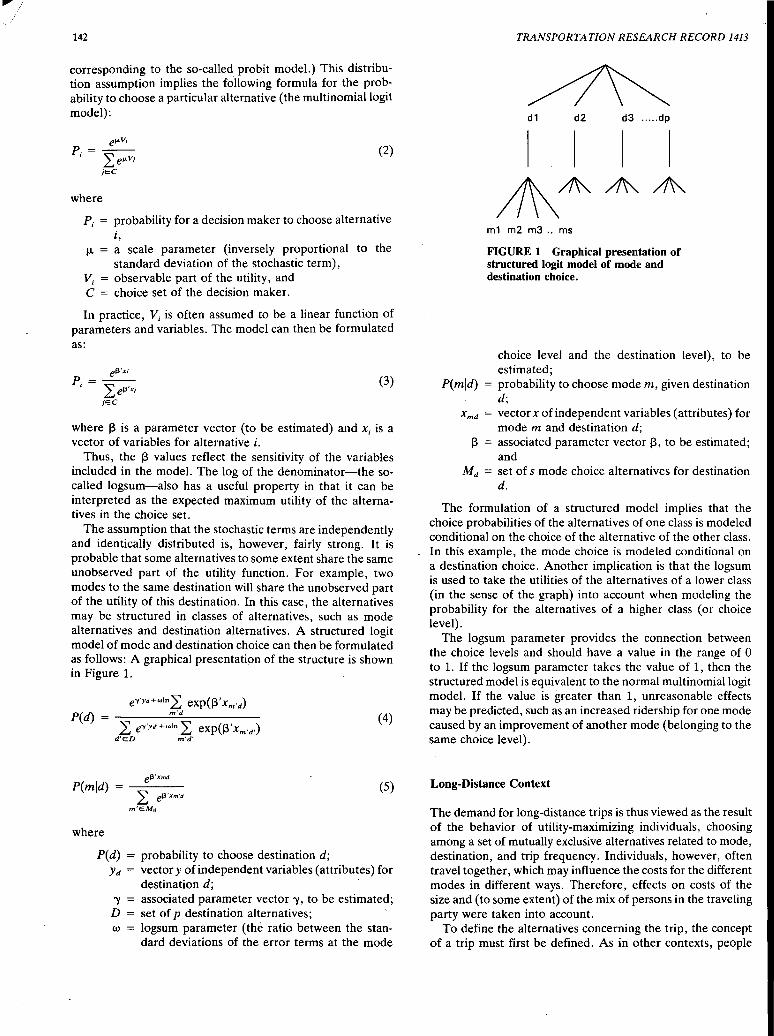
I 142

corresponding to the so-called probit model.) This distribu­tion assumption implies the following formula for the prob­ability to choose a particular alternative (the multinomial logit model):

(2)

where

P; = probability for a decision maker to choose alternative i,

µ = a scale parameter (inversely proportional to the standard deviation of the stochastic term),

V; = observable part of the utility, and C = choice set of the decision maker.

In practice, V; is often assumed to be a linear function of parameters and variables. The model can then be formulated as:

(3)

where ~ is a parameter vector (to be estimated) and X; is a vector of variables for alternative i.

Thus, the ~ values reflect the sensitivity of the variables included in the model. The log of the denominator-the so­called logsum-also has a useful property in that it can be interpreted as the expected maximum utility of the alterna­tives in the choice set.

The assumption that the stochastic terms are independently and identically distributed is, however, fairly strong. It is probable that some alternatives to some extent share the same unobserved part of the utility function. For example, two modes to the same destination will share the unobserved part of the utility of this destination. In this case, the alternatives may be structured in classes of alternatives, such as mode alternatives and destination alternatives. A structured logit model of mode and destination choice can then be formulated as follows: A graphical presentation of the structure is shown in Figure 1.

P(d)

P(mld)

where

e-y'yd+win 2: exp(Wxm·d) m'd

2: e-Y'Yd·+ ... in 2: exp(Wxm·d·) d'ED m'd'

2: eWxm'd

m'EMd

(4)

(5)

P(d) = probability to choose destination d; yd = vector y of independent variables (attributes) for

destination d; -y = associated parameter vector -y, to be estimated;

D = set of p destination alternatives; w = logsum parameter (the ratio between the stan­

dard deviations of the error terms at the mode

TRANSPORTATION RESEARCH RECORD 1413

d1 d2 d3 ..... dp

I I

~ m1 m2 m3 .. ms

FIGURE 1 Graphical presentation of structured logit model of mode and destination choice.

choice level and the destination level), to be estimated;

P(mld) = probability to choose modem, given destination d;

xmd = vector x of independent variables (attributes) for mode m and destination d;

~ = associated parameter vector~. to be estimated; and

Md = set of s mode choice alternatives for destination d.

The formulation of a structured model implies that the choice probabilities of the alternatives of one class is modeled conditional on the choice of the alternative of the other class. In this example, the mode choice is modeled conditional on a destination choice. Another implication is that the logsum is used to take the utilities of the alternatives of a lower class (in the sense of the graph) into account when modeling the probability for the alternatives of a higher class (or choice level).

The logsum parameter provides the connection between the choice levels and should have a value in the range of 0 to 1. If the logsum parameter takes the value of 1, then the structured model is equivalent to the normal multinomial logit model. If the value is greater than 1, unreasonable effects may be predicted, such as an increased ridership for one mode caused by an improvement of another mode (belonging to the same choice level).

Long-Distance Context

The demand for long-distance trips is thus viewed as the result of the behavior of utility-maximizing individuals, choosing among a set of mutually exclusive alternatives related to mode, destination, and trip frequency. Individuals, however, often travel together, which may influence the costs for the different modes in different ways. Therefore, effects on costs of the size and (to some extent) of the mix of persons in the traveling party were taken into account.

To define the alternatives concerning the trip, the concept of a trip must first be defined. As in other contexts, people

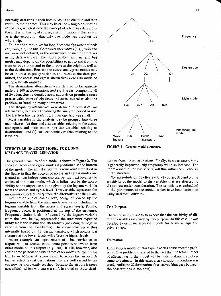
Alge rs

normally start trips in their homes, visit a destination and then return to their homes. This may be called a single-destination round trip, which is how the concept of a trip was defined in the analysis. This is, of course, a simplification of the reality, as is the assumption that only one mode was used on the whole trip.

Four mode alternatives for long-distance trips were defined: car, train, air, and bus. Combined alternatives (e.g., train and air) were not defined, as the occurrence of such alternatives in the data was rare. The utility of the train, air, and bus modes may depend on the possibilities to get to and from the train or bus station and to the airport at the origin as well as at the destination. Because the access and egress modes may be of interest as policy variables and because the data per­mitted, the access and egress alternatives were also modeled as separate alternatives.

The destination alternatives were defined to be approxi­mately 2,200 agglomerations and rural areas, comprising all of Sweden. Such a detailed zonal subdivision permits a more precise calculation of trip times and costs, but raises also the problem of handling many alternatives.

The frequency alternatives were defined to consist of two alternatives, to make a trip during the analyzed period or not. The fraction having made more than one trip was small.

Most variables in the analysis may be grouped into three main classes: (a) time and cost variables relating to the access and egress and main modes, (b) size variables relating to destinations, and ( c) socioeconomic variables relating to the travelers.

STRUCTURE OF LOGIT MODEL FOR LONG­DISTANCE TRAVEL BEHAVIOR

The general structure of the model is shown in Figure 2. The choice of access and egress modes is positioned at the bottom of the model. The actual structure is somewhat simplified in the figure in that the choices of access and egress modes are treated as two independent choices. At the next level is the choice of the main mode, which is influenced by the acces­sibility to the airport or station given by the logsum variable from the access and egress level. This variable represents the maximum expected utility from the alternatives at that level.

Destination choice comes next, being influenced by the logsum variable from the main mode level (also including the logsum variable from the access and egress level). Finally, frequency choice is positioned at the top of the structure. Frequency choice is also influenced by the logsum variable from the level below, representing the maximum expected utility from the destination alternatives (including the logsum variable from the level below). The entire structure is thus internally linked by the logsum variables, which means that changes at the lower levels will affect the higher levels.

As an example, an improvement of a bus service to an airport will, of course, cause some persons to switch from other modes to this airport (e.g., car). It will, however, also cause some persons to switch from other modes for their main trip to air because it is now easier to access the airport. A further effect is that destinations that are well served by air can now be more easily reached (because the airport is more accessible), which will cause a shift in travel to these desti-

0

Walk bicycle

01

Car

Car

1 +

02

Train Air

Public transport

Bus

Taxi

FIGURE 2 General model structure.

On

143

Frequency

Destination

Main mode

Access/egress mode

nations from other destinations. Finally, because accessibility is generally improved, trip frequency will also increase. The improvement of the bus service will thus influence all choices in the structure.

The magnitude of the effects will, of course, depend on the sensitivity of the model to the variables that are affected by the project under consideration. This sensitivity is embedded in the parameters of the model, which have been estimated using statistical software.

Trip Purpose

There are many reasons to expect that the sensitivity of dif­ferent variables may vary by trip purpose. In this case, it was decided to estimate separate models for business trips and private trips.

Estimation

Estimating a model of this type involves some specific prob­lems. One problem is related to the fact that the total number of alternatives in the model will be high, making it cumber­some to estimate. In this case, a stratification procedure was used, leading to 22 destination alternatives (that vary between the observations in the data).

/

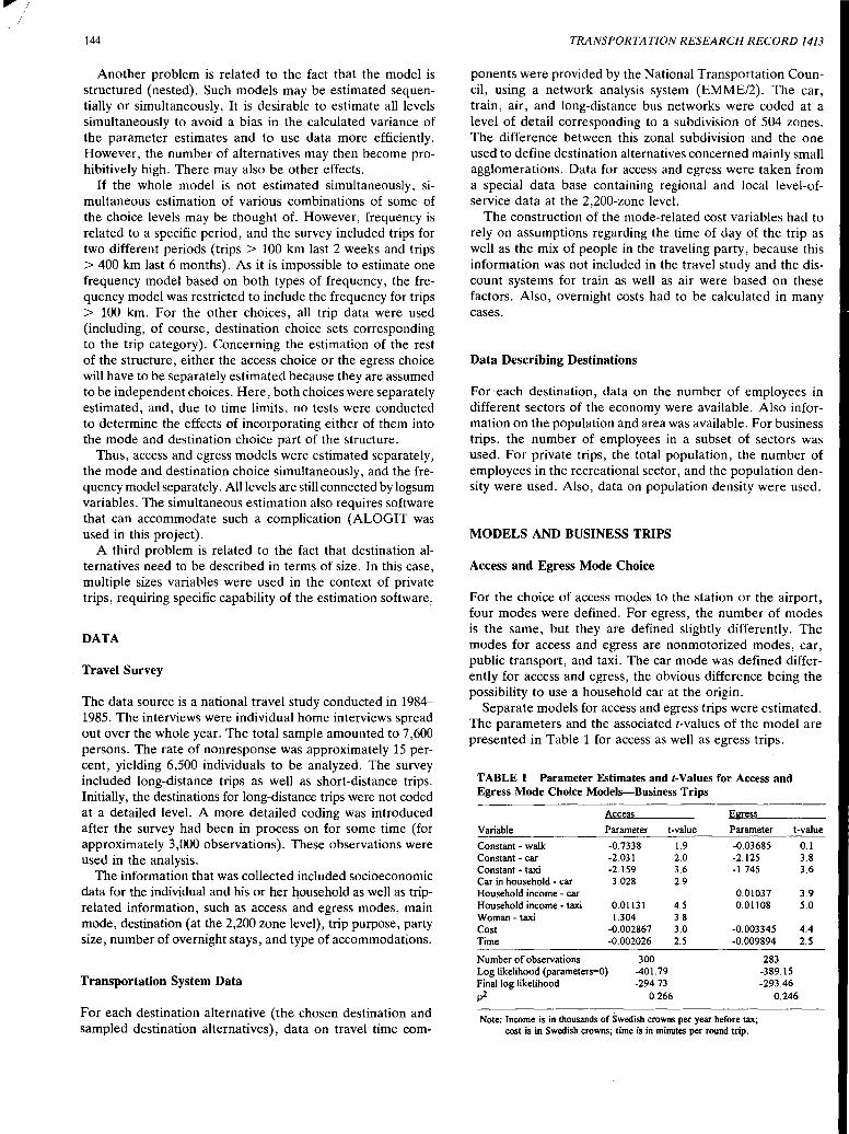
144

Another problem is related to the fact that the model is structured (nested). Such models may be estimated sequen­tially or simultaneously. It is desirable to estimate all levels simultaneously to avoid a bias in the calculated variance of the parameter estimates and to use data more efficiently. However, the number of alternatives may then become pro­hibitively high. There may also be other effects.

If the whole model is not estimated simultaneously, si­multaneous estimation of various combinations of some of the choice levels may be thought of. However, frequency is related to a specific period, and the survey included trips for two different periods (trips > 100 km last 2 weeks and trips > 400 km last 6 months). As it is impossible to estimate one frequency model based on both types of frequency, the fre­quency model was restricted to include the frequency for trips > 100 km. For the other choices, all trip data were used (including, of course, destination choice sets corresponding to the trip category). Concerning the estimation of the rest of the structure, either the access choice or the egress choice will have to be separately estimated because they are assumed to be independent choices. Here, both choices were separately estimated, and, due to time limits, no tests were conducted to determine the effects of incorporating either of them into the mode and destination choice part of the structure.

Thus, access and egress models were estimated separately, the mode and destination choice simultaneously, and the fre­quency model separately. All levels are still connected by logsum variables. The simultaneous estimation also requires software that can accommodate such a complication (ALOGIT was used in this project).

A third problem is related to the fact that destination al­ternatives need to be described in terms of size. In this case, multiple sizes variables were used in the context of private trips, requiring specific capability of the estimation software,.

DATA

Travel Survey

The data source is a national travel study conducted in 1984-1985. The interviews were individual home interviews spread out over the whole year. The total sample amounted to 7 ,600 persons. The rate of nonresponse was approximately 15 per­cent, yielding 6,500 individuals to be analyzed. The survey included long-distance trips as well as short-distance trips. Initially, the destinations for long-distance trips were not coded at a detailed level. A more detailed coding was introduced after the survey had been in process on for some time (for approximately 3,000 observations). These observations were used in the analysis.

The information that was collected included socioeconomic data for the individual and his or her household as well as trip­related information, such as access and egress modes, main mode, destination (at the 2,200 zone level), trip purpose, party size, number of overnight stays, and type of accommodations.

Transportation System Data

For each destination alternative (the chosen destination and sampled destination alternatives), data on travel time com-

TRANSPORTATION RESEARCH RECORD 1413

ponents were provided by the National Transportation Coun­cil, using a network analysis system (EMME/2). The car, train, air, and long-distance bus networks were coded at a level of detail corresponding to a subdivision of 504 zones. The difference between this zonal subdivision and the one used to define destination alternatives concerned mainly small agglomerations. Data for access and egress were taken from a special data base containing regional and local level-of­service data at the 2,200-zone level.

The construction of the mode-related cost variables had to rely on assumptions regarding the time of day of the trip as well as the mix of people in the traveling party, because this information was not included in the travel study and the dis­count systems for train as well as air were based on these factors. Also, overnight costs had to be calculated in many cases.

Data Describing Destinations

For 'each destination, data on the number of employees in different sectors of the economy were available. Also infor­mation on the population and area was available. For business trips, the number of employees in a subset of sectors was used. For private trips, the total population, the number of employees in the recreational sector, and the population den­sity were used. Also, data on population density were used.

MODELS AND BUSINESS TRIPS

Access and Egress Mode Choice

For the choice of access modes to the station or the airport, four modes were defined. For egress, the number of modes is the same, but they are defined slightly differently. The modes for access and egress are nonmotorized modes, car, public transport, and taxi. The car mode was defined differ­ently for access and egress, the obvious difference being the possibility to use a household car at the origin.

Separate models for access and egress trips were estimated. The parameters and the associated t-values of the model are presented in Table 1 for access as well as egress trips.

TABLE 1 Parameter Estimates and I-Values for Access and Egress Mode Choice Models-Business Trips

Access Egress

Variable Parameter t-value Parameter

Constant - walk -0.7338 1.9 -0.03685 Constant - car -2.031 2.0 -2.125 Constant - taxi -2.159 3.6 -1.745 Car in household - car 3.028 2.9 Household income - car 0.01037 Household income - taxi 0.01131 4.5 0.01108 Woman-taxi 1.304 3.8 Cost -0.002867 3.0 -0.003345 Time -0.002026 2.5 -0.009894

Number of observations 300 283 Log likelihood (parameters=O) -401.79 -389.15 Final log likelihood -294.73 -293.46

t-value

0.1 3.8 3.6

3.9 5.0

4.4 2.5

p2 0.266 0.246

Note: Income is in thousands of Swedish crowns per year before tax; cost is in Swedish crowns; time is in minutes per round trip.

Algers

The models exhibit approximately the same sensitivity to costs at the origin as at the destination. The sensitivity to time is, however, radically different, with a much greater sensitivity at the destination. A possible explanation is that the time spent at the origin does not have much alternative use as working time, because the access trip often takes place in the morning or evening, whereas the time at the destination often takes place during work hours.

The probability to use the more expensive modes is most likely related to the position of the traveler in the hierarchy and the economic strength of the company (or equivalent) where the person works. This is probably reflected in the salary of the person. However, person income was not re­ported in the survey, and household income is used as a proxy. Still, the effects are significant.

Choice of Main Mode and Destination

The parameter values for the mode and destination choice model are presented in Table 2. The model includes variables related to modes as well as to destinations. The model is simultaneously estimated, although with some important re­strictions. Generally, simultaneous estimation is preferable to sequential estimation. In this case, simultaneous estimation

145

increases the correlation between time variables, resulting in difficulties in estimating mode-specific time parameters.

Because a mode choice model could be estimated, the time and cost' parameters were used as input to the estimation of the mode and destination model, scaled by a specific "scale" parameter. The parameter values from the mode choice model are reported with t-values in brackets because they are not estimated in the mode and destination model. The scale pa­rameter, by which these made choice model parameter values should be multiplied, is reported separately with its associated t-value. The scale parameter is not significantly different from 1.

The cost parameters are segmented with regard to the type of worker. Full-time, salaried employees are likely to have higher values of time than others, which is reflected in the lower cost parameter for this category. The in-vehiele time parameter is much lower for train and bus as compared with car and air, which appears reasonable because working con­ditions are more favorable on trains and buses than in cars and aircraft. This was also found by Ridout and Miller (4). Waiting time has a significant influence if the frequency is higher than one train per 4 hr (in both directions).

The model also includes logsum parameters from the access mode model and from the egress mode model. The former is restricted to 1 because it otherwise would be larger than 1,

TABLE 2 Parameter Estimates and t-Values for Mode and Destination Choice Model-Business Trips

Model 1 Model2 Variable parameter t-value parameter t-value

Constant - train -2.898 4.4 -1.616 3.1 Constant - air -3.807 5.1 -2.564 4.2 Constant - bus -5.158 4.4 -6.024 5.3

In-vehicle/transfer time, car/air -0.0024 (5.8) --0.0024 (5.8) train/bus -0.0014 (4.9) --0.0014 (4.9)

Cost, full time salaried employees -0.00071 (3.2) --0.00071 (3.2) Cost, others -0.0013 (5.3) --0.0013 (5.3) Wait time, train/air< 240 min -0.0043 (2.5) --0.0043 (2.5) Parameter for generalised cost 1.090 10.3 1.083 10.4

Access (logsum) 1.0 (distance, km) --0.01183 2.8

Egress (logsum) 0.4912 3.5 (distance, km) --0.01421 2.7

Car in household - car 1.356 2.2 0.4306 0.8 Licenses per car - car -0.5038 2.2 --0.5547 2.5 Travelling party > 4 persons - bus 3.152 2.5 3.269 2.6

Destination in Stockholm - air 0.8568 3.4 0.9564 3.5 Destination in smaller towns - air -0.6861 2.2 --0.7420 2.4 Origin in Stockholm - air 1.165 4.5 l.395 5.2 Origin in medium sized towns - train 0.9884 3.9 0.9679 3.8

For all modes: Destination in Gothenburg -0.08027 0.3 --0.07147 0.3 Destination in medium size towns 0.2640 1.4 0.2896 1.5 Destination in smaller towns 0.05974 0.3 0.09827 0.4 Destination in villages -0.006948 0.0 --0.01682 0.1 Destination in rural areas 0.3109 0.9 0.3176 0.9

Size of destination (log of employees) 1.0 1.0 Logsum from mode choice 0.8410 8.0 0.8476 7.9

Number of observations 527 527 Log likelihood (0) -2267.48 - 2267.48 Final log likelihood -1472.33 -1483.52 p2 0.351 0.346

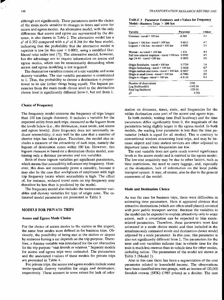
146

although not significantly. These parameters make the choice of the main mode sensitive to changes in times and costs for access and egress modes. An alternative model, with the only difference that access and egress are represented by the dis­tance, is also shown in Table 2. The alternative model has a p2 of 0.352 compared with a p2 of 0.346 for the base model, indicating that the probability that the alternative model is superior is low [in this case < 0.0001, using a modified like­lihood ratio index test (7)]. The alternative model, however, has the advantage not to require information on access and egress modes, which can be unnecessarily demanding when access and egress modeling is not required.

The destination variables consist of a size variable and some dummy variables. The size variable parameter is constrained to 1. Thus, the probability to choose a destination is propor­tional to its size (other things being equal). The logsum pa­rameter from the main-mode choice level to the destination choice level is significantly different from 0, but not from 1.

Choice of Frequency

The frequency model concerns the frequency of trips longer than 100 km (single distance). It includes a variable for the expected utility from such trips, measured as the logsum from the levels below (i.e., the destination, main mode, and access and egress levels). Zero frequency does not necessarily in­dicate nonmobility; it may well be the case that a number of shorter trips has taken place. Therefore, the model also in­cludes a measure of the attractivity of such trips, namely the logsum of destination zones within 100 km. However, this logsum measure is based on a destination choice model, con­taining only a distance parameter and size variables.

Both of these logsum variables get significant parameters, which means that accessibility influences trip frequency. How­ever, this does not necessarily prove a causality, because it may also be the case that workplaces of employees with high trip frequency locate where accessibility is high. The effect of, for instance, reduced travel costs on trip frequency may therefore be less than is predicted by the model.

The frequency model also includes the socioeconomic vari­ables and dummy variables for type of origin zone. The es­timated model parameters are presented in Table 3.

MODELS FOR PRIVATE TRIPS

Access and Egress Mode Choice

For the choice of access modes to the station or the airport, the same four modes were defined as for business trips. Ob­viously, the possibility of being met at the station or airport by someone having a car depends on the trip purpose. There­fore, a dummy variable was introduced for the car alternative for the trip purpose "visit friends or relatives." Separate models for access and egress trips were estimated. The parameters and the associated t-values of these models for private trips are presented in Table 4.

For private trips, the access and egress models include some mode-specific dummy variables for origin and destination, respectively. These account to some extent for lack of infor-

TRANSPORTATION RESEARCH RECORD 1413

TABLE 3 Parameter Estimates and I-Values for Frequency Model-Business Trips > 100 km

Variable Parameter

Constant - travel > I 00 km -6.069

Logsum > 100 km - travel > 100 km 0.6613 Logsum < 100 km - no travel > I 00 km 0.4585

Woman - no travel> 100 km 1.116 Full time salaried employee - travel > 100 km 0.9393 Age 24-45 - travel >I 00 km 0.5822

Origin Stockholm - travel> 100 km 0.7739 Origin Gothenburg - travel> 100 km 0.3828 Origin medium size towns - travel> 100 km -0.4807 Origin in small towns - travel> 100 km -0.7486 Origin in villages - travel > 100 km -0 .1116

Number of observations Log likelihood(O) Final log likelihood p2

1595 -1105.56

-329.36 0.702

t..qlue

H

4.7 3.6

4..4 4.0 2.6

l.6 0_7 L4 2.0 0.4

mation on distances, times, costs, and frequencies for the within destination zone part of the access~and egress trips.

In both models, waiting time (half headway) and the time parameters differ significantly from 0, the magnitude of the parameters being slightly larger in the egress model. In both models, the waiting time parameter is less than the time pa­rameter (which is equal for all modes). This is contrary to conventional wisdom concerning local trips, and may be be­cause airport and train station services are often adjusted to departure times when frequencies are low.

The cost variable does not quite reach normal significance levels in the access model and is omitted in the egress model. The low-cost sensitivity may be due to other factors, such as time restrictions, the need to carry luggage, and, especially at the destination, lack of information on the local public transport system. It may, of course, also be due to the general coarseness of the model.

Mode and Destination Choice

As was the case for business trips, there were difficulties in estimating time parameters. Here it appeared obvious that attractive destinations (which are often small places) covaried with poor public transport service. Because the variables in the model can be expected to explain attractivity only to some extent, such a covariation can be expected to bias mode­related parameters. Therefore, these parameters were first estimated in a mode choice model and then included ih the simultaneously estimated mode and destination choice model adjusted by a scale parameter. In this case, this parameter is also not significantly different from 1. The parameters for the time and cost variables indicate that in-vehicle time for the train is much less onerous than in-vehicle time for other modes, including railcar. The parameters of the model are shown in Table 5 (Model 1).

Also in this case there has been a segmentation of the cost parameter related to household income. The observations have been classified into two groups, with an income of 120,000 Swedish crowns (SEK) (1985 prices) as a divider. The cost

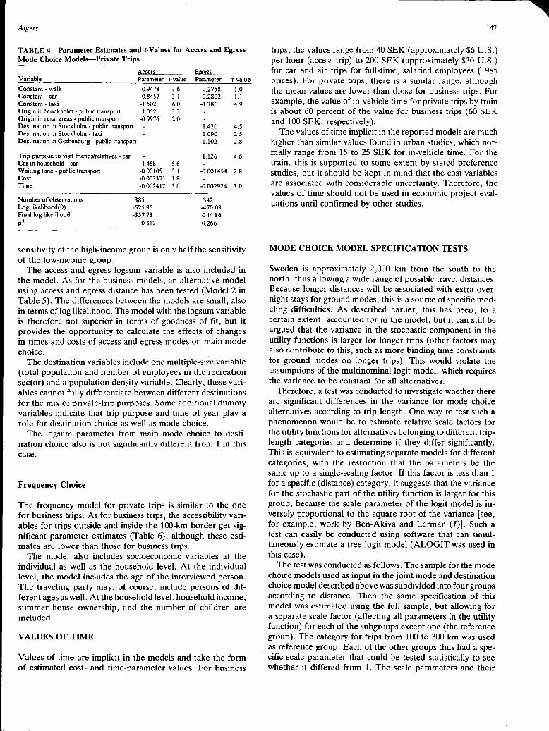
Algers

TABLE 4 Parameter Estimates and I-Values for Access and Egress Mode Choice Models-Private Trips

Access Ea-ess Variable Parameter t-value Pr.uneter t-value

Constant - walk -0.9478 3.6 -0.2758 1.0 Constant - car -0.8457 3.1 -0.2802 I.I Constant - taxi -1.502 6.0 -1.386 4.9 Origin in Stockholm - public transport 1.052 3.3 Origin in rural areas - public transport -0.9976 2.0 Destination in Stockholm - public transport - 1.420 4.5 Destination in Stockholm - taxi 1.090 2.5 Destination in Gothenburg - public transport - 1.102 2.8

Trip purpose to visit friends/relatives - car 1.126 4.6 Car in household - car 1.468 5.6 Waiting time - public transport -0.001051 3.1 -0.001454 2.8 Cost -0.003371 1.8 Time -0.002412 3.0 -0.002924 3.0

Number of obseivations 385 342 Log likelihood(O) -525.95 -470.08 Final log likelihood -357.73 -344.86 p2 0.312 0.266

sensitivity of the high-income group is only half the sensitivity of the low-income group.

The access and egress logsum variable is also included in the model. As for the business models, an alternative model using access and egress distance has been tested (Model 2 in Table 5). The differences between the models are small, also in terms of log likelihood. The model with the logsum variable is therefore not superior in terms of goodness of fit, but it provides the opportunity to calculate the effects of changes in times and costs of access and egress modes on main mode choice.

The destination variables include one multiple-size variable (total population and number of employees in the recreation sector) and a population density variable. Clearly, these vari­ables cannot fully differentiate between different destinations for the mix of private-trip purposes. Some additional dummy variables indicate that trip purpose and time of year play a role for destination choice as well as mode choice.

The logsum parameter from main mode choice to desti­nation choice also is not significantly different from 1 in this case.

Frequency Choice

The frequency model for private trips is similar to the one for business trips. As for business trips, the accessibility vari­ables for trips outside and inside the 100-km border get sig­nificant parameter estimates (Table 6), although these esti­mates are lower than those for business trips.

The model also includes socioeconomic variables at the individual as well as the household level. At the individual level, the model includes the age of the interviewed person. The traveling party may, of course, include persons of dif­ferent ages as well. At the household level, household income, summer house ownership, and the number of children are included.

VALVES OF TIME

Values of time are implicit in the models and take the form of estimated cost- and time-parameter values. For business

147

trips, the values range from 40 SEK (approximately $6 U.S.) per hour (access trip) to 200 SEK (approximately $30 U.S.) for car and air trips for full-time, salaried employees (1985 prices). For private trips, there is a similar range, although the mean values are lower than those for business trips. For example, the value of in-vehicle time for private trips by train is about 60 percent of the value for business trips (60 SEK and 100 SEK, respectively).

The values of time implicit in the reported models are much higher than similar values found in urban studies, which nor­mally range from 15 to 25 SEK for in-vehicle time. For the train, this is supported to some extent by stated preference studies, but it should be kept in mind that the cost variables are associated with considerable uncertainty. Therefore, the values of time should not be used in economic project eval­uations until confirmed by other studies.

MODE CHOICE MODEL SPECIFICATION TESTS

Sweden is approximately 2,000 km from the south to the north, thus allowing a wide range of possible travel distances. Because longer distances will be associated with extra over­night stays for ground modes, this is a source of specific mod­eling difficulties. As described earlier, this has been, to a certain extent, accounted for in the model, but it can still be argued that the variance in the stochastic component in the utility functions is larger for longer trips (other factors may also contribute to this, such as more binding time constraints for ground modes on longer trips). This would violate the assumptions of the multinominal logit model, which requires the variance to be constant for all alternatives.

Therefore, a test was conducted to investigate whether there are significant differences in the variance for mode choice alternatives according to trip length. One way to test such a phenomenon would be to estimate relative scale factors for the utility functions for alternatives belonging to different trip­length categories and determine if they differ significantly. This is equivalent to estimating separate models for different categories, with the restriction that the parameters be the same up to a single-scaling factor. If this factor is less than 1 for a specific (distance) category, it suggests that the variance for the stochastic part of the utility function is larger for this group, because the scale parameter of the logit model is in­versely proportional to the square root of the variance [see, for example, work by Ben-Akiva and Lerman (J)]. Such a test can easily be conducted using software that can simul­taneously estimate a tree logit model (ALOGIT was used in this case).

The test was conducted as follows. The sample for the mode choice models used as input in the joint mode and destination choice model described above was subdivided into four groups according to distance. Then the same specification of this model was estimated using the full sample, but allowing for a separate scale factor (affecting all parameters in the utility function) for each of the subgroups except one (the reference group). The category for trips from 100 to 300 km was used as reference group. Each of the other groups thus had a spe­cific scale parameter that could be tested statistically to see whether it differed from 1. The scale parameters and their

148 TRANSPORTATION RESEARCH RECORD 1413

TABLE 5 Parameter Estimates and t-Values for Mode and Destination Choice Model-Private Trips

Model 1 Model 2 Variable parameter t-value parameter t-value

Constant - train -1.044 3.2 0.1915 1.2 Constant - air -2.434 9.0 -0.9014 3.6 Constant - bus -1.011 4.9 -1.085 5.3

Invehicle time car/bus/jetplane -0.002676 (12.3) -0.002676 (12.3) Invehicle time train (normal/sleep) -0.001117 (4.3) -0.001117 (4.3) Invehicle time train - railcar -0.002727 (3.6) -0.002727 (3.6) lnvehicle time air (prop. aircraft) -0.003415 (1.8) -0.003415 (1.8)

Cost, household income <120 000 SEK -0.001762 (7.3) -0.001762 (7.3) Cost, household income >120 000 SEK -0.0008363 (2.9) -0.0008363 (2.9)

Waiting time (half headway) -0.002197 (2.0) -0.002197 (2.0) Number of transfers - train -0.2512 (4.5) -0.2512 (4.5) Number of transfers - air ~0.3729 (2.9) -0.3729 (2.9)

Scale parameter 1.061 18.6 l.106 19.3

Access/egress logsum 0.5324 4.7

Access/egress distance -0.01162 4.5

Car in household - car 2.088 12.5 1.913 11.8 Licenses per car - car -1.804 8.9 -1.724 8.5

Age < 18 years - car -0.9010 5.8 -0.8962 5.7 Age > 64 years - air -1.295 3.1 1.393 3.4 Trip purpose recreation - car 0.4961 3.5 0.6939 5.1 Trip purpose recreation - bus 1.780 8.6 1.934 9.4 Trip purpose summer house - car 0.9862 3.3 1.147 3.8

Destination in Stockholm -0.5552 3.2 -0.4169 2.5 Destination in Gothenburg -0.1770 0.9 -0.1191 0.6 Destination in medium size towns 0.2063 1.3 0.1944 1.2 Destination in smaller towns 0.1201 0.9 0.1135 0.8 Destination in villages 0.1925 1.7 0.1927 1.7

Recr. trip in June/July - villages 0.4852 3.3 0.4889. 3.3 Visit trip in June/July - rural areas -0.5104 2.0 -0.5152 2.0

Population density in dest. zone -0.04371 6.8 -0.04390 6.8 Logsum from mode choice 0.8912 16.3 0.8620 16.6

Size variables: Population 1. 1. Number of employees in recreation branch, for recreation 4.837 25.1 4.841 25.1 (not exponentiated)

Number of observations 1846 1846 Log likelihood (0) -7492.01 -7492.01 Fmal log likelihood -5733.41 -5733.23 p2 0.234 0.234

associated standard errors are shown for business trips as well as for private trips in Table 7.

The meaning of these scale parameters is that the estimated parameter values (not shown here) are to be multiplied by these factors when applying the model to mode choice alter­natives in a certain distance category. This means that the sensitivity to variable changes will be larger when the scale parameter is larger than 1, and reverse (everything else being equal).

As shown in Table 7, there are large differences between the·different subgroups in the business model, although only the scale parameter for the third category is significantly dif­ferent from 1. For private trips, the differences are not large, and none of the scale factors is significantly different from 1.

The results suggest that it is reasonable to include the full range of travel distances in the mode choice model for private trips (with the current specification), and that the model for business trips needs to be improved to meet the requirements for the multinomial logit model. These results may have an interest per se, although the specification of the joint mode and destination choice model (or the other models) was not analyzed in this particular way.

Further complexity of the model structure was also not tested within the reported project. The data are, however, still subject to research. A specification test that was con­ducted later (suggested by a referee) split mode choice into two levels: (a) the choice between the car and shared modes and (b) choice between shared modes. Although significantly

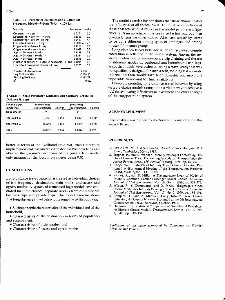
Algers

TABLE 6 Parameter Estimates and t-Values for Frequency Model-Private Trips > 100 km

Variable Parameter t-valu:

Constant - l+ trips -2.057 2.0 Logsum trip > 100 km - I+ trips 0.1566 2.'.: Logsum trip< 100 km - no trip 0.2453 4.4 Household income - I+ trip 0.002457 2.:: Origin in Stockholm - I+ trip 0.4212 1.9 Origin in rural areas - l+ trip -0.4648 3.C: Age < 19 years - l+ trip 0.3538 1.8 Age 19-24 years - l+ trip 0.5264 3.G Age >64years-l+trip -0.3635 2.1 Number of persons< 12 years in household - I+ trip-0.1034 1.4 Household owns summerhouse - I+ trip 0.5725 5.1

Number of observations Log likelihood(O) Final log likelihood p2

2700 -3196.57 -1182.73

o.63u

TABLE 7 Scale Parameter Estimates and Standard Errors for Distance Groups

Tra\-el distance (single way)

Up to 300 km

301 - 600 km

601-900 km

901-

Business trigs scale parameter

1.0

1.382

0.6250

0.8692

Private trigs std error scale parameter std error

1.0

0.258 0.8897 0.0706

0.140 0.8985 0.0793

0.214 0.8844 0.102

better in terms of the likelihood ratio test, such a structure implied poor cost parameter estimates for business trips and affected the parameter estimates of the private trips model only marginally (the logsum parameter being 0.8).

CONCLUSIONS

Long-distance travel behavior is treated as individual choices of trip frequency, destination, main mode, and access and egress modes. A system of structured logit models was esti­mated for these choices. Separate models were estimated for business trips and private trips. The model exercise shows that long-distance travel behavior is sensitive to the following:

• Socioeconomic characteristics of the individual and of the household,

• Characteristics of the destination in terms of population and employment,

• Characteristics of main modes, and • Characteristics of access and egress modes.

149

The model exercise further shows that these characteristics are influential at all choice levels. The relative importance of these characteristics is reflect in the model parameters. Spe­cifically, train in-vehicle time seems to be less onerous than in-vehicle time for other modes. Also, cost sensitivity seems to be quite different among types of employes and among household income groups.

Long-distance travel behavior is, of course, more compli­cated than is reflected in the model system. Among the ne­glected behavioral phenomenon are trip chaining and the use of different modes on outbound and homebound trip legs. Also, the models were estimated using a travel study that was not specifically designed for such a task, yielding less accurate information than would have been desirable and making it impossible to account for time availability.

However, modeling long-distance travel behavior by using discrete choice models seems to be a viable way to achieve a tool for evaluating infrastructure investment and other changes of the tra11sportation system.

ACKNOWLEDGMENT

This analysis was funded by the Swedish Transportation Re-search Board.

REFERENCES

1. Ben-Akiva, M., and S. Lerman. Discrete Choice Analysis. MIT Press, Cambridge, Mass., 1985.

2. Stopher, P., and J. Prashker. Intercity Passenger Forecasting: The Use of Current Travel Forecasting Procedures. Transportation Re­search Forum, Proc., 17th Annual Meeting, 1976, pp. 67-75.

3. Koppelman, F. Models of Intercity Travel Choice Behavior. Pre­sented at 68th Annual Meeting of the Transportation Research Board, Washington, D.C., 1989.

4. Ridout, R., and E. Miller. A Dissaggregate Logit of Model of Intercity Common Carrier Passenger Modal Choice. Canadian Journal of Civil Engineering, Vol. 16, No. 4, 1989, pp. 568-575.

5. Wilson, F., S. Damodaran, and D. Innes. Disaggregate Mode Choice Models for Intercity Passenger Travel in Canada. Canadian Journal of Civil Engineering, Vol. 17, No. 2, 1990, pp. 184-191.

6. Ramjerdi, F., and A. Madslien. Long Distance Travel Choice Behavior, the Case of Norway. Presented at the 6th International Conference on Travel Behavior, Quebec, 1991.

7. Horowitz, J. L. Statistical Comparison of Non-Nested Probabilis­tic Discrete Choice Models. Transportation Science, Vol. 17, No. 3, 1983, pp. 319-350.

Publication of this paper sponsored by Committee on Traveler Behavior and Values.