Embed Size (px)
Citation preview

-Page 1-
TRAVEL TIME STUDY OF AUCKLAND ARTERIAL ROAD NETWORK USING GPS DATA
John J.J.S. Sia, Philip C.H. Ching, Prakash Ranjitkar*
Department of Civil and Environmental Engineering, The University of Auckland, Private
Bag 92019, Auckland, New Zealand, E-mail: [email protected]
Abstract: Travel time information is important for transportation planning, route guidance as
well as congestion management purposes. It is also one of the most important measures for
evaluating the performance of road networks. This paper reports a study conducted in
Auckland City to investigate the level of congestion on three major arterial routes. Travel
time data was collected using an instrumented vehicle equipped with GPS receiver during
morning peak hours based on average car method. The Level of Service (LOS) concept
proposed in Highway Capacity Manual 2000 was used to determine the level of congestion.
The sample size required for reliable estimation of travel time was determined based on
confidence interval method.
Key Words: Travel Time, GPS, Level of Service, Traffic Congestion
* Corresponding author
1. INTRODUCTION
Travel time-based measures, such as mean travel time, mean speed, and delay, are easy to
understand for transportation professionals as well as to general public including commuters,
business persons and consumers. These measures are important to evaluate the performance
of road networks. There are an increasing number of transportation agencies switching to
travel time measures to monitor traffic condition (Quiroga, 2000).
BECA Infrastructure has been conducting travel time studies on motorways and arterial
routes in all major cities of New Zealand as a part of annual traffic monitoring program for
the New Zealand Transport Agency (previously Transit New Zealand) since 2002 (Wu and
Ensor, 2007). These studies employ the congestion indicator (CGI), which is calculated using
a methodology developed by Austroads, the Ministry for the Environment and Transit New
Zealand to measure level of congestion in New Zealand cities and compare them with
Australian cities (Ministry for the Environment and Transit New Zealand, 2001).
Global Positioning System (GPS) is an emerging technology with wide applications in
transportation engineering in different areas such as traffic data collection, congestion
management studies and car-following analysis (Ranjitkar, 2004, Ranjitkar et al, 2005,
Ranjitkar and Nakatsuji, 2006). This paper presents a further application of the GPS
technology in transport to study travel time and delay on three major arterial routes within
Auckland City. This study is based on the level of service (LOS) concept presented in
Highway Capacity Manual (HCM) 2000.
The issues discussed in this paper are as follows:
- The number of test runs required for the reliable estimation of the performance
measures.

-Page 2-
- The performance evaluation of three major arterial routes in Auckland City based on
LOS concept proposed in HCM 2000.
- The level of congestion trend in Auckland City.
The following section covers details on the study area, average car method used in this study
for data collection, test car instrumentation details, arrangements for test runs and data
processing. The performance measures used in this study are briefly described in Section 3.
The discussion on number of test runs required for reliable estimation of the performance
measures in Section 4 and the analysis results are presented in Section 5. Finally, the research
outcomes are discussed in the last section.
2. DATA COLLECTION
2.1 Study Area
Three major arterial routes were selected in Auckland for this study. These routes connect the
central business district (CBD) with major commercial, industrial and high density residential
zones. They also serve as the common alternatives to motorway routes and state highways.
They were:
Great South Route: an industrial and commercial zone with bus lane included along
the route and linked to the Southern Motorway 1.
Mission Bay Route: a highly variable route where majority of traffic is controlled by
roundabout / signs instead of traffic signals.
New North Route: a high density residential and schools zone area, with main
arterials linked to South-East, Great North Road and Motorway 16.
Table 1 presents the route definition and route ID that will be used in this report. Figure 1
shows the arterial routes. For each route, data was collected on the city bound and outward
bound directions.
2.2 Average-Car Method
Average-car method is the preferred method for travel time study (Robertson et al, 1994) and
was employed in this study to collect travel time and delay data. This method is less
restrictive than the floating-car method in which the driver tries to “float” with traffic flow
by attempting to safely pass as many vehicles as pass the test vehicle. In the average-car
method, the test vehicle’s driver travels according to the driver’s judgment of the average
speed of the traffic stream.
2.3 Test Car
The GPS system used in this study consisted of a GPS device with roof mounted antenna, a
PDA (HP-IPAQ) and a computer program GPS2PDA developed by Jamar Technologies.
The performance of the test vehicle is not influential as the posted speed limit for all routes
was 50 km/hr. The GPS records data at one-second intervals. The accuracy of the
measurement data depends on the quality of GPS signals received, which is represented by
an index called Horizontal Dilution of Precision (HDOP). There are two modes in which the
GPS system used can operate namely single and differential modes. Under differential mode,
the device yields sub metre level of accuracy, while under single mode the error in position
measurement can go up to ± 3 metre, which is sufficient for this type of study. A limitation
of GPS is that signal loss can occur in areas with tall buildings, or other overhead
obstructions. This was not a factor in this study because the routes were in open areas.

-Page 3-
Table 1 Route ID and definition
Routes Direction Route ID
Great South Road City Bound GSR_CB
South Bound GSR_SB
Mission Bay Route City Bound MBR_CB
East Bound MBR_EB
New North Road City Bound NNR_CB
West Bound NNR_WB
Figure 1 Arterial routes chosen for this study (highlighted in black)
2.4 Test Run Methodology
The data was collected during morning peak from 7:30am to 9:30am. This peak time
duration was established from previous studies conducted by Wu and Ensor (2007) and
Beca, Parsons Brinckerhoff and Andrew O'Brien & Associates (2005). The control points,
usually signalized intersections on route, were pre-determined. Section lengths varied from
0.2 km to 2.5 km. Practice runs were driven several times to familiarize the driver and
assistant with the routes and tasks to perform. The data collection was started before 7am
allowing at least 30 minutes time for instrumental set up and satellite fixing for the GPS unit.
Data were collected from Monday to Wednesday, during the university semester (July-
September, 2008), excluding public holidays and inclement weather.
The speed driven is determined by the driver based on the surrounding vehicle flow. The
assistant in the front passenger seat records the locations of nodes (pre-determined) by
clicking a button on the PDA connected with the GPS. The GPS unit displays position, speed,
HDOP and other information. The assistant also records any incidents that might have
occurred during data collection period in a data collection log book. This includes time,
location and description of the incident. The quality of GPS data depends on signal strength,
which can be checked from time to time for HDOP values. The assistant also monitors and
records any loss of signals during the data collection. Most of the time during the data
collection, observed HDOP values were two or less, representing either single or differential
mode, which is sufficient for this type of study.

-Page 4-
2.5 Data Processing
The GPS data recorded in a memory stick was downloaded in to a computer for data
processing and analysis. The data were first checked for consistency. Some data required
manual correction involving addition or removal of nodes mainly due to human error for
instance some times the assisting person forgot to click the GPS button at some nodes. These
were corrected later by comparing the GPS co-ordinates of the nodes obtained under free
flow conditions (in early morning before 4am). In addition the nodes were compared to the
other runs from the same direction to check for consistency. All data with incidents were
excluded for analysis e.g. on Mission Bay Route in City Bound direction there was a bus
broken down causing abnormal delays; as a result this run was ignored during the processing
stage. The data was then corrected using PC-Travel Time software developed by Jamar
Technologies. This software estimates travel time data (in seconds), number of stops (in
miles per hour which was converted to kilometres per hour) and delay (in seconds).
3. PERFORMANCE MEASURES The road sections were classified as either class III or class IV to determine the LOS
depending on the Free Flow Speed (FFS) obtained. The sections with FFS 50km/h or greater
were classified as Class III, sections with FFS below 50km/h were classified as Class IV.
After classification, the mean speed for the section was compared with Table 2 to determine
the LOS. To identify the worst sections within the routes, the sections organised into the
respective LOS ratings. After which the sections were rated based on percentage of FFS
obtained during the data runs.
4. NUMBER OF TEST RUNS
The common range recommended in the literatures for the accuracy of average speed varies
from ±1.6km/h to ±4.8km/h for before and after studies (Qiang, 2007, Turner and Holdener,
1995). The traditional method is to use Standard Deviation (SD) for sample sizes (Turner and
Holdener, 1995). This method has been widely accepted and used since 1995; however the
SD method is out of date. Qiang (2007) updated the SD method by including Confidence
Intervals (CI) and conducted several trials to verify the accuracy of the results. The new
method is used in this study. The literature proposed a requirement of 10 to 15 runs for
reliability and acceptable accuracy. This investigation was conducted to determine what
sample size is required for the Auckland traffic conditions.
Table 2 LOS Chart for Arterial Roads
Urban Street Class I II III IV
Range of Free-Flow
Speed (FFS) 90 to 70 km/h 70 to 55 km/h 55 to 50 km/h 55 to 40 km/h
Typical FFS 80 km/h 65 km/h 55 km/h 45 km/h
LOS Average travel speed km/h
A > 72 > 59 > 50 > 41
B > 56-72 > 46-59 > 39-50 > 32-41
C > 40-56 > 33-46 > 28-39 > 23-32
D > 32-40 > 26-33 > 22-28 > 18-23
E > 26-32 > 21-26 > 17-22 > 14-18
F < 26 < 21 < 17 < 14
Source: EXHIBIT 15-2. URBAN STREET LOS BY CLASS (HCM 2000)

-Page 5-
The number of test runs we have conducted in this study are based on the lowest limit of
accuracy for before and after studies, that of ±4.8km/h with an 80% confidence Interval. The
formula used is 2
2a
E
σZn (1)
Where:
n: is the required number of runs
2aZ : is the standard normal distribution value for a given Confidence Interval (CI)
: is the standard deviation for the sample
E: is the allowable error for the sample, E varies from ±1.6Kph to ±4.8Kph
The standard normal distribution values for different confidence interval are as follows:
(CI=80%) (CI=90%) (CI=95%)
Z = 1.29 Z = 1.65 Z = 1.96
5. ANALYSIS RESULTS
5.1 Required number of runs
The determination of the required number of runs is focused on two fields, both of which are
in the city bound direction. The first is for the whole route while the second is on section by
section analysis of the three routes.
Figure 2 presents the number of runs conducted and required for each route for different
levels of accuracy. As can be seen in this figure, all of the routes meet the minimum accuracy
requirements of ± 4.8 km/h with 80% confidence interval. All but the GSR_SB route meet
the interim level of accuracy of ±2.4kph and CI of 90%. This result would suggest that, the
minimum number of runs for such study should be no less than five runs. However, from the
three city bound routes, 10 runs is the ideal for practical accuracy.
Figure 3 presents section-wise results for MBR_CB route. It appears that there are at least
three sections that exceeded the minimum requirements: sections 4, 6 and 10. The
variability for section 4 is due to the presence of two intersection controls within a short
section length (around 250 m). The main problem is the intersection of Kohimarama Road,
St Johns Road and St Heliers Bay Road. This short section provides service to the
MBR_CB route flows and the Greenlane Road flows as well as the Newmarket Road
flows and the Southern Motorway 1 flows. As this is unavoidable, it is recommended for
future studies that the MBR_CB route take no less than 10 runs. The high run requirement
for section 10 is due to the signalised intersection and the corresponding lane arrangement
which frustrates free flow.
Table 3 presents the number of stops and delays for the MBR_CB route for different runs.
The number of stops can vary significantly due to lane under utilisation, resulting in higher
run requirements. Little can be done to the methodology to avoid this problem.
Figure 4 presents section-wise results for the GSR_CB route. There are several sections
which exceed the minimum requirements, namely, sections 2, 5, 6, 7 and 8. Although there is

-Page 6-
high variability for the sections, it may be due to bunching of vehicles at different sections. In
addition, sections 7 and 8 are short sections with lengths of 260m and 500m respectively. The
short section length combined with controlled intersections means that variations, such as
number of stops, can cause large differences in average speed. Where no stops occur there are
significant increases in mean speed, highlighted in Figure 5.
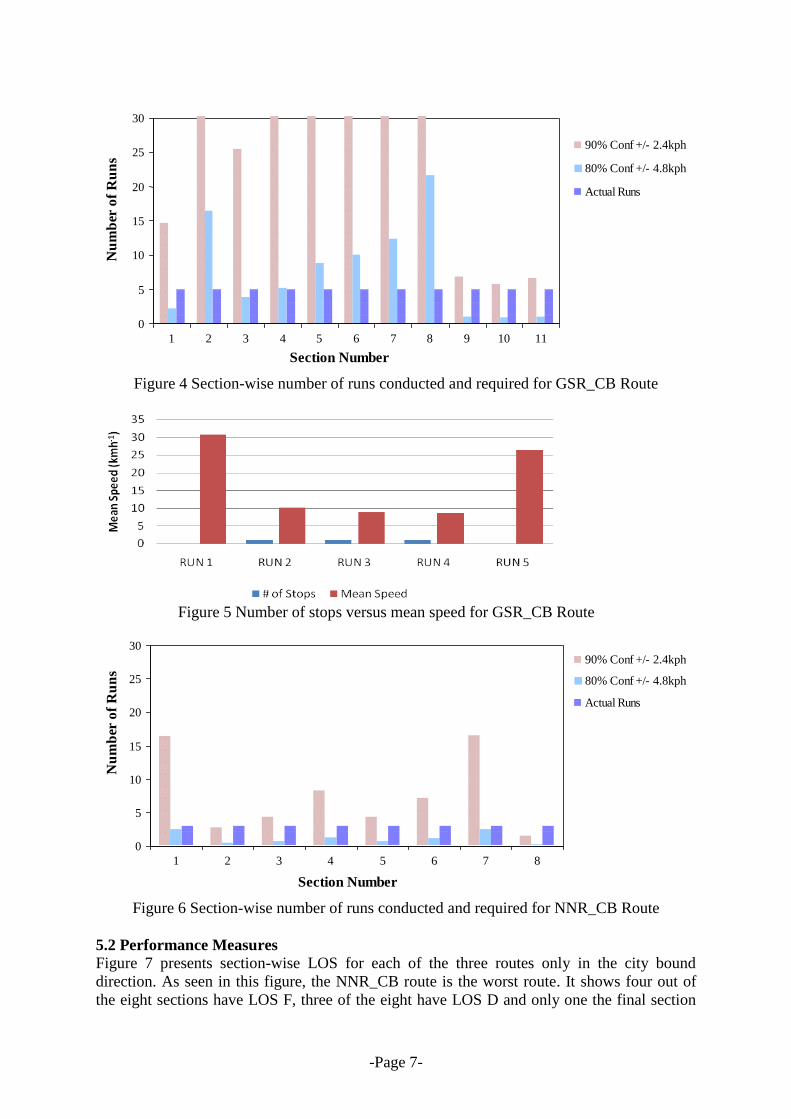
Figure 6 presents section-wise results for NNR_CB route. While MBR_CB and GSR_CB
routes had high levels of variation, the NNR_CB route is relatively consistent. All sections
are within the minimum levels of accuracy. This is due to the uniform flow produced as
routes near their capacity. With 50% of the route in LOS F and 38% in LOS D, there was
little variation in mean speeds. As traffic flow on the NNR_CB route approaches close to its
capacity, the data observed are more close to normal.
Table 3 Number of Stops and Delays in Section 10
MBR_CB RUN 1 RUN 2 RUN 3
# of stops 3 0 5
Delay (sec) 143 14 302
GSR_CB GSR_SB MBR_CB MBR_EB NNR_CB NNR_WB
0
5
10
15
20
25
30
Routes
Nu
mb
er o
f R
un
s
95% Conf +/- 1.6kph
90% Conf +/- 2.4kph
80% Conf +/- 4.8kph
Actual Runs
Figure 2 Number of runs conducted and required for each route
MBR_CB Route
0
5
10
15
20
25
30
1 2 3 4 5 6 7 8 9 10 11
Section Number
Nu
mb
er o
f R
un
s
90% Conf +/- 2.4kph
80% Conf +/- 4.8kph
Actual Runs
Figure 3 Section-wise number of runs conducted and required for MBR_CB Route
-Page 7-
GSR_CB Route
0
5
10
15
20
25
30
1 2 3 4 5 6 7 8 9 10 11
Section Number
Nu
mb
er o
f R
un
s
90% Conf +/- 2.4kph
80% Conf +/- 4.8kph
Actual Runs
Figure 4 Section-wise number of runs conducted and required for GSR_CB Route
Figure 5 Number of stops versus mean speed for GSR_CB Route
NNR_CB Route
0
5
10
15
20
25
30
1 2 3 4 5 6 7 8
Section Number
Nu
mb
er o
f R
un
s
90% Conf +/- 2.4kph
80% Conf +/- 4.8kph
Actual Runs
Figure 6 Section-wise number of runs conducted and required for NNR_CB Route
5.2 Performance Measures
Figure 7 presents section-wise LOS for each of the three routes only in the city bound
direction. As seen in this figure, the NNR_CB route is the worst route. It shows four out of
the eight sections have LOS F, three of the eight have LOS D and only one the final section

-Page 8-
has LOS C. The second worst route of the three is the MBR_CB route, in terms of congestion.
Three sections have LOS F indicating serious congestion problem in those sections. The
MBR_CB route have a spread of LOS ratings with one LOS E, one LOS D, five LOS C and
two sections rated as LOS B.
LOS Maps provide a quick summary of congestion on the routes. However, the mean speed
for each section provides another perspective on which to assess congestion and is easier to
understand. We computed the mean speed as follows:
TimeTravelAverage
SectionofLengthSpeedMean (2)
Where length of section is measured in kilometres and average travel time is measured in
hours. The latter term is computed as average of travel time taken during the test runs to
traverse the section of road. Figure 8 presents section-wise map of the mean speed for all of
the three routes. The results highlight the same conclusion as drawn from the LOS maps.
Figure 9 presents section-wise average delay (in minutes) for each of the three routes in the
city bound direction. The delay term here represents the total time spent by the vehicle along
a section travelling at or below 5 km/h speed. The average delay for each section was
calculated as follows:
n
Delay
delayAverage
n
1 (3)
Where n is number of test runs conducted. MBR_CB route, Section 1, on Pakuranga Road,
between Ti Rakau Drive and Lagoon Drive observed to have the highest average delay
compared with all other sections. This section of road experiences an average delay of 8.7
minutes.
5.3 Performance Based Ranking of Road Sections
Table 4 presents 15 worst performing sections based on FFS rating for all of the three routes.
The FFS percentile rating calculated using the following formula:
Figure 7 LOS for all three routes in city bound direction during AM peak period

-Page 9-
Figure 8 Mean speed for all three routes in city bound direction during AM peak period
Figure 9 Delay (in minutes) for all three routes in city bound direction during AM peak
period
x100speedflowfree
speedmean%Rating (4)
In order to determine the ratings, the sections were organised into LOS classes. The mean
speed for the section was then divided by the free flow speed (using equation 4). The result is
a rating, in percentile terms, of existing performance relative to the achievable FFS.
There are still some issues with using HCM2000 LOS rating, take for example number 9 in
Table 4, highlighted in red. The rating is 69.2% yet it is classified as LOS F. This is a direct
result of the rating system; Class IV sections cover all FFS below 50. For this section FFS
speed was 16.58 the result of a short section and non-green wave configured traffic controls.
The alternative method of ranking the LOS is based on mean speed over posted speed, for
this study the speed is 50kph presented in Table 5. This method allows for a direct

-Page 10-
comparison between sections. Highlighting the previous example (shown in red in Table 4)
the LOS is better represented showing that it is now the third worst section in the study.
However, this method is less relevant as it does not take into account free flow speed.
Therefore for the purposes of ranking, the use of equation 2 is recommended.
From the results in Tables 4 and Table 5, the worst section is section 9. This section is on the
Mission Bay City Bound Route located between Apirana Ave and St Heliers Bay Road. From
Table 4 the worst route is the NNR_CB with four out of eight sections being LOS F.
Conversely NNR_WB is the best route, as four of the eight sections are LOS A and the other
four LOS B. The low LOS for NNR_CB is a key issue, as high flows have been observed to
travel mainly on one lane, due to high numbers of buses using the left lane. This may require
future road widening schemes on the city bound direction.
Table 4 Rating of Route Sections from Worst
LOS to Best
RANKING ORDER % MEAN SPEED OVER FFS ACHIEVED
Km/h LOS FFS Rating % Section Route Section
10.46 F 49.08 21.3% Apriana Ave - St Heliers Bay Rd MBR_CB 9
11.96 F 50.05 23.9% St Georges - Blockhouse Bay Rd NNR_CB 2
11.10 F 44.26 25.1% Ti Rakau Dr - Jellicoe Rd MBR_EB 1
14.00 F 54.72 25.6% Symonds – Alfred MBR_CB 1
13.20 F 50.21 26.3% Woodward Rd - Mt Albert Rd NNR_CB 4
14.97 F 51.66 29.0% Symonds – Alfred MBR_EB 11
14.48 F 49.57 29.2% Khyber Pass Rd - Alfred St NNR_CB 8
16.68 F 50.69 32.9% St Lukes Rd - Sandringham Rd NNR_CB 6
11.47 F 16.58 69.2% Broadway – Remuera GSR_SB 6
Table 5 Ranking based on Mean speed over 50kph
RANKING ORDER % MEAN SPEED OVER 50 Km/h
Km/h LOS FFS Rating % Section Route Section
10.46 F 49.08 20.9% Apriana Ave - St Heliers Bay Rd MBR_CB 9
11.10 F 44.26 22.2% Ti Rakau Dr - Jellicoe Rd MBR_EB 1
11.47 F 16.58 22.9% Broadway – Remuera GSR_SB 6
11.96 F 50.05 23.9% St Georges - Blockhouse Bay Rd NNR_CB 2
13.20 F 50.21 26.4% Woodward Rd - Mt Albert Rd NNR_CB 4
14.00 F 54.72 28.0% Symonds – Alfred MBR_CB 1
14.13 E 34.76 28.3% Khyber Pass - Mountain Rd GSR_CB 9
14.48 F 49.57 29.0% Khyber Pass Rd - Alfred St NNR_CB 8
14.29 E 42.49 28.6% K-road - Khyber Pass GSR_CB 10
6. DISCUSSION
We have reported in this paper a pilot study conducted based on HCM (2000) LOS concept
on three major arterial routes in Auckland City to measure the level of congestion
experienced on these routes during peak hours. The number of test runs conducted in this
study has met the requirements for before and after studies. The results are consistent and are
within acceptable statistical boundaries. As a result of this pilot study it is suggested that to
build greater confidence in the results, five additional runs should be the minimum and, 10
runs being ideal.

-Page 11-
NNR_CB route was found to have least variations might be due to the fact that flows on this
route were close the capacity. The maximum number of required runs computed for the route
was one. The worst section, in terms of LOS, was on the MBR_CB route section 1, between
Ti Rakau Drive and Jellicoe Drive. This section is facing the highest delay of 8.7 minutes.
Although MBR_CB route has two worst sections, NNR_CB is the worst route as 50% of this
route is performing at LOS F, and 38% at LOS D. Observations during data collection
indicate problems due to capacity. The installation of an additional lane may be warranted as
the peak flow is limited to one lane due to the presence of an AM bus lane.
It is recommended that for future studies every intersection be recorded as a node. This will
allow for easier computation of travel time data and may reduce the required number of runs.
Combined with an increased number of nodes and increased sample size, we might be able to
achieve an accuracy level of ±1.6kph with CI of 95%. We have investigated delay averaged
over sections; it might be useful to brake down the average delay into minutes per kilometre
travelled. This would allow for a comparison with ongoing Transit CGI based monitoring of
delay. A further research is needed to look into the correlation between section length and
number of runs required, with special consideration into the road type. The concept behind
road type shall be determined based on traffic volumes and density of intersection controls.
7. REFERENCES
Beca, Parsons Brinckerhoff and Andrew O'Brien & Associates (2005) Sothern Motorway
Travel Demand Management - Existing Conditions Report. Auckland, Transit New
Zealand.
Highway Capacity Manual (2000) Transportation Research Board, Ed., National Research
Council, Washington D.C.
Hunter, M. P., Wu, S. K. and Kim, H. K. (2006) Practical Procedure to Collect Arterial
Travel Time Data using GPS-Instrumented Test Vehicles, Transportation Research
Record, Vol. 1978, 160-168.
Mauricio, I. C., Santos, R. C., Diliman, Q. C. and Philippines, P. (2003) Travle time and
delay analysis using GIS and GPS, Proceedings of the Eastern Asia Society for
Transportation Studies, Vol. 4.
Ministry for the Environment and Transit New Zealand (2001) Indicators of the
environmental effects of transport-Travel time indicator.
Qiang, L. (2007) Arterial Road Travel Time Study using Probe Vehicle Data. PhD
Dissertation, Nagoya University.
Quiroga, C. A. (2000) Performance measures and data requirements for congestion
management systems. Transportation Research Part C, Vol. 8, 287-306.
Ranjitkar, P. (2004) “Experimental Assessment of Microscopic Traffic Flow Models Based
on RTK GPS Data”, Ph.D. Dissertation, Hokkaido University.
Ranjitkar, P., Nakatsuji, T., Azuta, Y., Asano, M. and Kawamura, A. (2005) A Contemporary
Reassessment of GM Car Following Model using RTK GPS Data. Journal of
Infrastructure Planning and Management, No. 793/IV-68, pp. 121-132.
Ranjitkar, P. and Nakatsuji, T. (2006) Advances in microscopic traffic data collection using
instrumented vehicles. Traffic Engineering and Control, Vol. 47, No. 4, pp. 147-151.
Robertson, H.D., Hummer, J.E. and Nelson, D.C. (1994) Manual of Transportation
Engineering Studies, Chapter 4: Travel Time and Delay Studies, pp. 52-68.
Turner, S. M. and Holdener, D. J. (1995) Probe vehicle sample sizes for real-time
information: the Houston experience. Proceedings of Vehicle Navigation and Information
Systems Conference, 1995.

-Page 12-
Wu, D. and Ensor, M. (2007) Auckland Traffic System Performance Monitoring Report -
March 2007.