Embed Size (px)
Citation preview
GMAT 4010 - Thesis B
UNSW School of Surveying and Spatial Information Systems
Traversing the UNSW campus using
Terrestrial Photogrammetry
Author: Jarrod Braybon
z3219882
Supervisor - Dr. Bruce Harvey
Co-supervisors - Yincai Zhao and Professor John Trinder
Date: October 21st 2011

ii
Declaration of Academic Integrity
iii
Abstract
This thesis presents the findings of a comparison between the results presented by Gabriel
Scarmana at the 2010 Fèdèration Internationale des Gèometres (FIG) and the results of an
independent test. It is to be determined if Scarmana’s presented results of using close range
photogrammetry to traverse around buildings can be successfully replicated by an inexperienced
user.
Experimental procedures were kept constant where possible to maintain consistency and the same
software program, Photomodeler Pro, was used for processing. An increase in the quality of camera
was one change to the project parameters, it was anticipated this would improve positional
accuracy.
Over a distance of 140m, 52 photographs were taken and 284 reference points were identified and
processed. Upon completion of the traverse the largest positional error was calculated to be 0.651m
from the coordinates measured using traditional surveying methods. This error occurred at the
furthest point from the origin. The traverse was reprocessed as an incomplete loop with the
positional errors increasing to over 2 m. From this it was determined that a closed loop provides
considerably more accurate positional results.
The 0.651 m positional error over 140 m is significantly better than that suggested by Scarmana (1 m
error for every 150 m of traverse). This improvement in accuracy is believed to be due to the higher
quality camera used in this project
From the results obtained in this thesis it can be concluded that Scarmana’s results can be
reproduced by an inexperienced user to a similar standard. Several areas of potential improvement
to the method were identified including: the use of portable targets; investigating the affect of angle
geometry on positional accuracy; and the use of more control points to improve three dimensional
accuracy.
With improvements to accuracy, photogrammetry may become a useful alternative surveying
technique in the future.
iii
Table of Contents Abstract .................................................................................................................................................. iii
List of Figures .......................................................................................................................................... v
List of Tables ........................................................................................................................................... v
Acknowledgements ................................................................................................................................ vi
1. Introduction .................................................................................................................................... 1
2. Background ..................................................................................................................................... 3
2.1 Photogrammetry ..................................................................................................................... 3
2.1.1 Close Range Photogrammetry ........................................................................................ 5
2.1.2 Photogrammetry Process................................................................................................ 7
2.1.3 Factors affecting Photogrammetry ................................................................................. 8
2.1.4 Scaling Photogrammetry ................................................................................................. 9
2.2 FIG paper ................................................................................................................................. 9
2.2.1 Location ......................................................................................................................... 10
2.2.2 Camera and Software.................................................................................................... 10
2.2.3 Process .......................................................................................................................... 11
2.2.4 Results ........................................................................................................................... 13
2.3 Camera Calibration ............................................................................................................... 13
2.4 Camera Parameters .............................................................................................................. 14
2.4.1 Principal Distance or Focal Length ................................................................................ 14
2.4.2 Principal Point ............................................................................................................... 14
2.4.3 Indicated Principal Point - Xp Yp..................................................................................... 15
2.4.4 Radial Distortions - K1 K2 K3 ........................................................................................... 15
2.4.5 Decentring Distortions - P1 P2 ....................................................................................... 16
3. Camera Calibration ....................................................................................................................... 18
3.1 Project Camera ...................................................................................................................... 18
3.1.1 Camera Calculations ...................................................................................................... 18
3.1.2 Field Of View Calculation .............................................................................................. 19
3.1.3 Pixel Size Calculation ..................................................................................................... 20
3.1.4 View Angle Calculation.................................................................................................. 20
3.2 Photomodeler Pro ................................................................................................................. 21
3.3 Calibration ............................................................................................................................. 22
3.3.1 Camera Calibration Results ........................................................................................... 22
3.3.2 Photomodeler Calibration ............................................................................................. 22
iv
3.3.3 Calibration Problems ..................................................................................................... 23
3.3.4 Image Acquisition .......................................................................................................... 25
3.3.5 Camera Calibration Results using Photomodeler Pro ................................................... 25
3.3.6 Photomodeler Comparison ........................................................................................... 27
3.3.7 iWitness Camera Calibration ......................................................................................... 27
3.3.8 iWitness Results and Comparisons ............................................................................... 28
4. Field work ...................................................................................................................................... 30
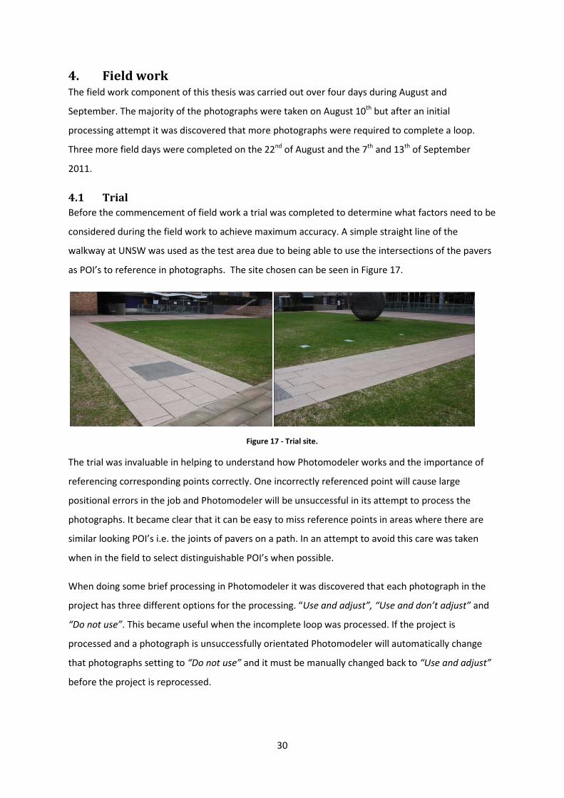
4.1 Trial ....................................................................................................................................... 30
4.2 Location ................................................................................................................................. 31
4.3 Field work .............................................................................................................................. 31
4.4 Processing in Photomodeler ................................................................................................. 33
4.5 Coordinate system ................................................................................................................ 35
4.6 Total Station Check ............................................................................................................... 36
5. Results and Analysis ...................................................................................................................... 37
5.1 Full Loop ................................................................................................................................ 37
5.1.1 Point accuracies ............................................................................................................ 37
5.1.2 AutoCAD Comparisons .................................................................................................. 39
5.1.3 Point Residuals .............................................................................................................. 42
5.1.4 Point Angles .................................................................................................................. 43
5.2 Incomplete Loop ................................................................................................................... 44
5.2.1 Point accuracies ............................................................................................................ 45
5.2.2 AutoCAD Comparisons .................................................................................................. 46
5.2.3 Point Residuals .............................................................................................................. 48
5.3 Comparisons ......................................................................................................................... 48
6. Conclusions ................................................................................................................................... 50
6 References .................................................................................................................................... 53
7. Bibliography .................................................................................................................................. 55
8. Appendix ....................................................................................................................................... 56
8.1 Camera Features ................................................................................................................... 56
8.2 FOV calculation ..................................................................................................................... 57
8.3 View angle calculation .......................................................................................................... 58
v
List of Figures Figure 1 - Single point and Multipoint Triangulation. ............................................................................. 3
Figure 2 - Multiple POI’s from multiple camera images. ........................................................................ 4
Figure 3 - Analogue Photogrammetry System................................................................................... .... 5
Figure 4 - Digital Photogrammetry System................... .......................................................................... 5
Figure 5 - Factors influencing accuracy of photogrammetric measurements. ....................................... 8
Figure 6 - Gabriel Scarmana's camera projections. .............................................................................. 12
Figure 7 - Results obtained by Scarmana. ............................................................................................. 13
Figure 8 - Elements of a lens system. .................................................................................................... 14
Figure 9 - Radial Distortions. ................................................................................................................. 15
Figure 10 - Misalignment of the components of a lens system. ........................................................... 16
Figure 11 - Decentring Distortion values .............................................................................................. 16
Figure 12 - Referencing Tutorial in Photomodeler. .............................................................................. 21
Figure 13 - Photomodeler calibration grid and camera locations. ....................................................... 23
Figure 14 - Image used for Photomodeler calibration. ......................................................................... 25
Figure 15 - Residuals produced by Photomodeler calibration. ............................................................. 27
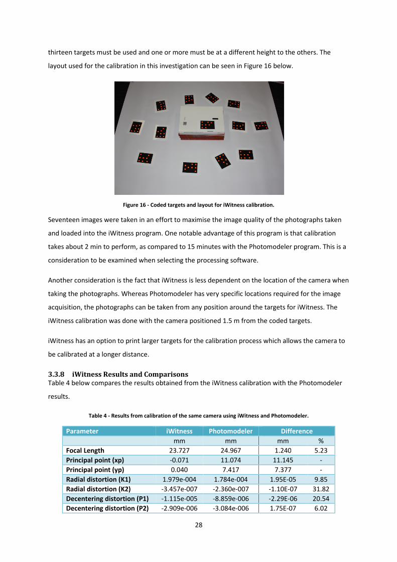
Figure 16 - Coded targets and layout for iWitness calibration. ............................................................ 28
Figure 17 - Trial site. .............................................................................................................................. 30
Figure 18 - The Hut Dance Studio ......................................................................................................... 31
Figure 19- Displayed photograph values. ............................................................................................. 32
Figure 20 - Camera setup positions ...................................................................................................... 33
Figure 21 - Epipolar lines intersection. ................................................................................................. 34
Figure 22 - Processing results. .............................................................................................................. 35
Figure 23 - Control point coordinates. .................................................................................................. 35
Figure 24 - Control network. ................................................................................................................. 36
Figure 25 - Plotted error bars for easting and northing . ...................................................................... 37
Figure 26 - Easting Errors. ..................................................................................................................... 40
Figure 27 - Northing Errors. .................................................................................................................. 41
Figure 28 - Height Errors. ...................................................................................................................... 42
Figure 29 - Incomplete loop. ................................................................................................................. 44
Figure 30 - Plotted easting and northing error bars. ............................................................................ 45
Figure 31 - ENH errors for incomplete loop. ......................................................................................... 47
List of Tables Table 1 - Calibration Results. ................................................................................................................ 22
Table 2 - Results from Photomodeler calibration. ................................................................................ 25
Table 3 - Result comparisons between two Photomodeler calibrations of the same camera. ............ 27
Table 4 - Results from calibration of the same camera using iWitness and Photomodeler................. 28
Table 5 - Control coordinates. .............................................................................................................. 36
Table 6 - Positional precisions. .............................................................................................................. 38
Table 7 - Coordinate Comparison. ........................................................................................................ 39
Table 8 - Top 5 worst residuals. ............................................................................................................ 42
Table 9 - Top 5 worst angles. ................................................................................................................ 44
Table 10 - Precision Comparisons. ........................................................................................................ 46
Table 11 - AutoCAD Comparison........................................................................................................... 47
Table 12 - Incomplete loop residuals. ................................................................................................... 48

vi
Acknowledgements I would like to thank my supervisor Dr Bruce Harvey for all of his help and time as well as providing
guidance for the duration of this thesis. I would also like to thank Professor John Trinder and Yincai
Zhao for their considerable assistance as co-supervisors.
A special thank you to Paul Wigmore for his assistance as a field hand when completing the field
work component of this thesis.
1
1. Introduction At the 2010 Fèdèration Internationale des Gèometres (FIG) conference in Sydney, Gabriel Scarmana
proposed the use of terrestrial photogrammetry as an alternative method for traversing buildings
and using non-stereo convergent images to coordinate features. Scarmana traversed a distance of
approximately 450m around a city block located within the business district of Surfers Paradise with
“the plan to measure a set of 80 points of interest (i.e. public assets such as traffic signs, bus
shelters, street lights and major trees) located along the streets” (Scarmana, 2010).
Images were taken every 10-15 metres as Scarmana moved forward around the city loop with
shorter distances used when entering a turn at street corners. Three well defined marks were
established through the use of a Leica TC2002 total station and used as coordinates for the initial
control points of the network. Control marks assist in initial orientation and scaling of a project.
Sequential photographs are then connected by the identification of suitable points of interest. A
suitable point of interest must have a clearly defined edge or centre where the same point can be
confidently and accurately be marked consistently on several different photographs. The best
objects to use as points of interest are edges of windows, road centrelines or the intersection of
cracks in the footpath.
Scarmana used the Windows-based photogrammetry software ‘Photomodeler Pro’ from EOS
Systems Inc. to process the results. This program takes 2D photograph images and creates a 3D
representation of the image complete with 3D coordinates. Photomodeler is designed in such a way
that the user need not be an expert in the photogrammetry field.
Using this method, Scarmana found that photogrammetry could be successfully used as a simple
alternative method of surveying, with an accuracy error of approximately 1 m for every 150 m
traversed.
This thesis presents the results of an independent test of Scarmana’s proposal. The aim of the
project was to determine if the method could be reproduced to the same standard by a non-
photogrammetry expert. It is not suggested that his proposal or results are flawed in any way.
Attempts were made to minimise changes to the method to ensure consistency, however one
notable improvement to the project was the quality of the camera used.
The author started the project relatively inexperienced in the field of photogrammetry. Over the
course of the research a better understanding of the technique, including its advantages and
limitations, was gained. Trial field work, software tutorials, learning about the features and settings

2
of the camera all assisted with the successful completion of the project. Much of the discussion
focuses on lessons learned from the project, and future recommendations for anyone working in the
field with a limited understanding of photogrammetry.
3
2. Background
2.1 Photogrammetry Photogrammetry is a coordination technique that utilises methods of image measurement and
interpretation to derive and determine the shape, location and orientation of an object or ‘point of
interest’ (POI) from one or more photographs of that object. (Luhman et al, 2006) A POI of an image
refers to a distinct area or object in a photograph that can be clearly defined and referenced. Some
examples of points that could be used as a POI are:
• Building corners
• Window edges
• Street signs
• Footpaths
• Road markings
When selecting a POI to reference it is important to use all areas of the image including both
foreground and background areas. The focus of this investigation was close range photogrammetry,
where the object or POI is less than 300 metres from the origin of the camera.
Using multiple two dimensional photographs, three dimensional (3D) coordinates of a POI are
produced by analysing the position of each photograph relative to each other. The photogrammetric
process can be applied to any situation where the object in question can be photographically
recorded.
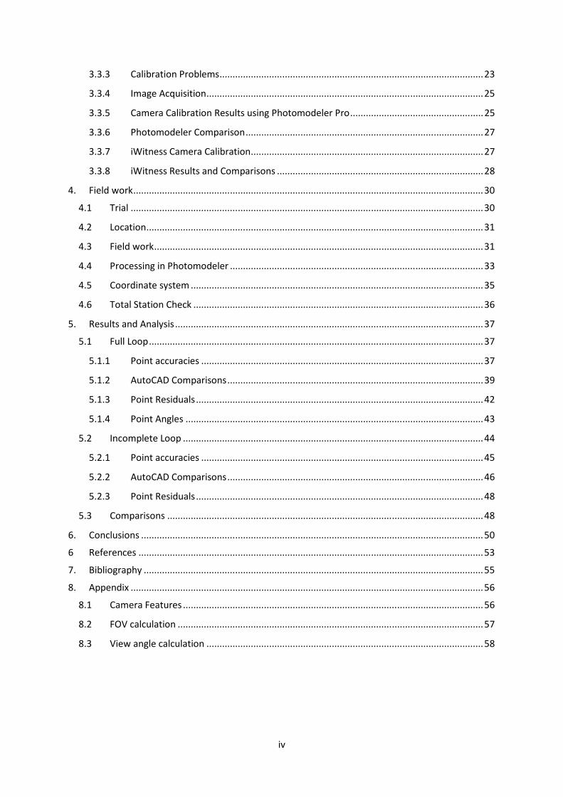
The fundamental principle behind photogrammetry is a process called “triangulation”. Triangulation
is used when two or more photographs with common features or POI’s visible in both images are
taken from different locations. Rays (or lines of sight) are created from the origin of the camera to
the POI and are mathematically intersected to produce 3D coordinates for the POI.
Figure 1 - Single point and Multipoint Triangulation (Geodetic Surveys, 2006).
A bundle triangulation occurs where a numerical fit is simultaneously calculated for all distributed
images (or bundles of rays). The bundle adjustment makes use of known input control coordinates
4
and, using scales and rays to common POI’s, is able to adjust a coordinate system for all images. In a
complex system of equations an adjustment technique does the following (Luhman et al, 2006):
1. Estimates the 3D coordinates of each referenced POI
2. Orientates each photograph
3. Detects gross errors and outliers
Triangulation is the principle used by theodolites to produce 3D point measurements:
By mathematically intersecting converging lines in space, the precise location of the point
can be determined. However, unlike theodolites, photogrammetry can measure multiple
points at a time with virtually no limit on the number of simultaneously triangulated points.
(Geodetic Surveys, 2006)
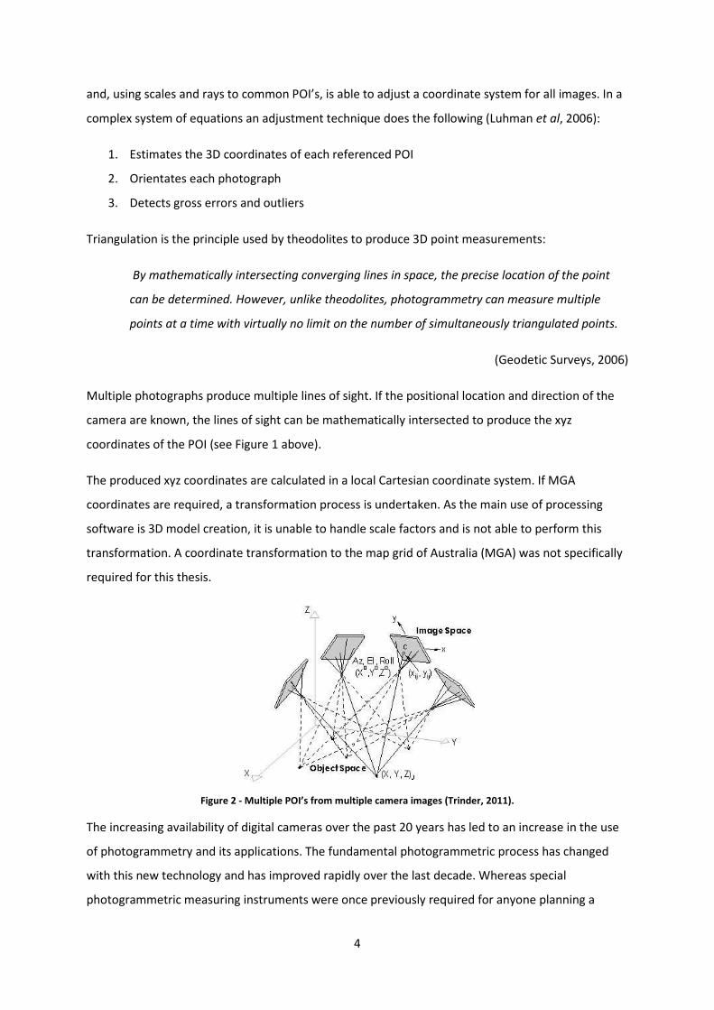
Multiple photographs produce multiple lines of sight. If the positional location and direction of the
camera are known, the lines of sight can be mathematically intersected to produce the xyz
coordinates of the POI (see Figure 1 above).
The produced xyz coordinates are calculated in a local Cartesian coordinate system. If MGA
coordinates are required, a transformation process is undertaken. As the main use of processing
software is 3D model creation, it is unable to handle scale factors and is not able to perform this
transformation. A coordinate transformation to the map grid of Australia (MGA) was not specifically
required for this thesis.
Figure 2 - Multiple POI’s from multiple camera images (Trinder, 2011).
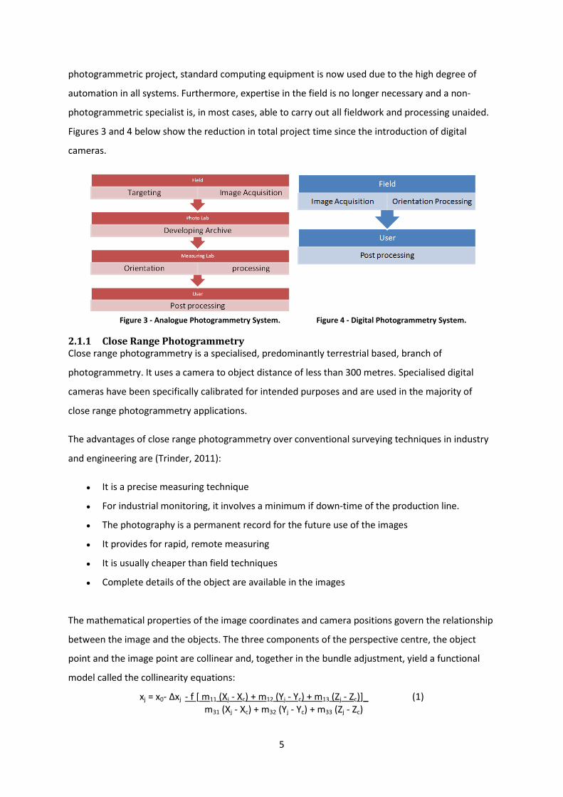
The increasing availability of digital cameras over the past 20 years has led to an increase in the use
of photogrammetry and its applications. The fundamental photogrammetric process has changed
with this new technology and has improved rapidly over the last decade. Whereas special
photogrammetric measuring instruments were once previously required for anyone planning a
5
photogrammetric project, standard computing equipment is now used due to the high degree of
automation in all systems. Furthermore, expertise in the field is no longer necessary and a non-
photogrammetric specialist is, in most cases, able to carry out all fieldwork and processing unaided.
Figures 3 and 4 below show the reduction in total project time since the introduction of digital
cameras.
Figure 3 - Analogue Photogrammetry System. Figure 4 - Digital Photogrammetry System.
2.1.1 Close Range Photogrammetry
Close range photogrammetry is a specialised, predominantly terrestrial based, branch of
photogrammetry. It uses a camera to object distance of less than 300 metres. Specialised digital
cameras have been specifically calibrated for intended purposes and are used in the majority of
close range photogrammetry applications.
The advantages of close range photogrammetry over conventional surveying techniques in industry
and engineering are (Trinder, 2011):
• It is a precise measuring technique
• For industrial monitoring, it involves a minimum if down-time of the production line.
• The photography is a permanent record for the future use of the images
• It provides for rapid, remote measuring
• It is usually cheaper than field techniques
• Complete details of the object are available in the images
The mathematical properties of the image coordinates and camera positions govern the relationship
between the image and the objects. The three components of the perspective centre, the object
point and the image point are collinear and, together in the bundle adjustment, yield a functional
model called the collinearity equations:
xj = x0- Δxj - f [ m11 (Xj - Xc) + m12 (Yj - Yc) + m13 (Zj - Zc)]_ (1)
m31 (Xj - Xc) + m32 (Yj - Yc) + m33 (Zj - Zc)

6
yj = y0- Δyj - f [ m21 (Xj - Xc) + m22 (Yj - Yc) + m23 (Zj - Zc)]_ (2)
m31 (Xj - Xc) + m32 (Yj - Yc) + m33 (Zj - Zc)
Where (Trinder, 2011):
• xj, yj are image coordinates.
• x0 , y0 are displacement coordinates between the actual origin of the image coordinates and
the true origin defined by the principal point.
• Δxj , Δyj are the corrections applied to the image coordinates for systematic errors in image
geometry.
• f is the camera principal distance or focal length.
• Xj , Yj , Zj are the object coordinates of point j.
• Xc , Yc , Zc , are the coordinates of the camera in the object space coordinate system.
• m11 ... m33 are the elements of a 3 x 3 orthogonal rotation matrix M which is a function of 3
rotations of the camera coordinate system, ω, φ, κ about the 3 axes x, y and z respectively.
There are two collinearity equations produced for each point on a photograph but as there is three
unknown’s xyz and only two equations we are unable to solve for the object coordinates. However,
when we have a common image in multiple photographs we have four or more equations, two from
each image, which allows us to solve for the three unknown values of xyz
The collinearity equations describe the fundamental mathematical model for photogrammetric
mapping. They demonstrate the relationship between the image and the object coordinate systems.
With the collinearity equations, the bundle adjustment can perform and solve the two basic
functions of photogrammetric mapping:
• Resection: In resection, the position and orientation of an image is determined by placing a
set of at least three points with known coordinates in the object frame as well as in the
image frame.
• Intersection: In intersection, two images with known position and orientation are used to
determine the coordinates in the object frame of features found on the two images
simultaneously, employing the principle of stereovision.
Both the resection and intersection method are implemented through an iterative least squares
adjustment.

7
2.1.2 Photogrammetry Process
Due to digital advancements, modern processes are usually highly automated and require minimal
referencing and calculations from the user. Below is a simplified outline of the four major stages of a
photogrammetric coordination project.
1. Recording
• Targeting - when selecting the areas for an image it must first be determined what POI’s will
be visible in the photograph. It is important to have approximately 25-30 visible POI’s in each
image to help improve automation and increase accuracy (Scarmana, 2011). Using a large
number of POI’s will help link the rays within each photograph for the bundle adjustment,
increasing redundancy and improving accuracy. Automation can be further improved by
using coded targets.
• Determination of control points or scaling lengths - in order to give the POI meaningful
coordinates, a coordinate system must be defined. This is usually done by implementing
control points (3 or more) into the first photograph. Each control point should not have
more than one identical coordinate to another control point (i.e. the xy, yz and xz
coordinates should not match for any control points). Having one of the x,y or z coordinates
matching is acceptable. Control points also help with scaling and orientating the
photographs but are not essential. Other methods of scaling of the photographs can be seen
in Section 2.1.3 below (Luhman et al, 2006).
2. Pre-processing
• Computation - calculation of control points with a total station to help coordinate the
photographs (Luhman et al, 2006).
3. Orientation
• Measurement of image points - identification and measurement of control points and
common POI’s. (Points of interest that are visible in two or more images)
• Approximation - a rough calculation is given for unknown parameters and POI’s based on the
control points and the scale calculated. This is crucial as it yields approximate values for the
bundle adjustment to work with.
• Bundle adjustment - adjustment program which simultaneously calculates parameters of
both interior (camera) and exterior (photograph) orientation. The object point coordinates
are also calculated by the bundle adjustment (Luhman et al, 2006).
• Removal of outliers - any gross errors are detected and removed (Luhman et al, 2006).
4. Measurement and Analysis
• Single point measurement - 3D coordinates are created for all referenced POI’s.
8
• Graphical plotting - final coordinated POI’s are easily mapped or made available for a CAD
program (Luhman et al, 2006).
2.1.3 Factors affecting Photogrammetry
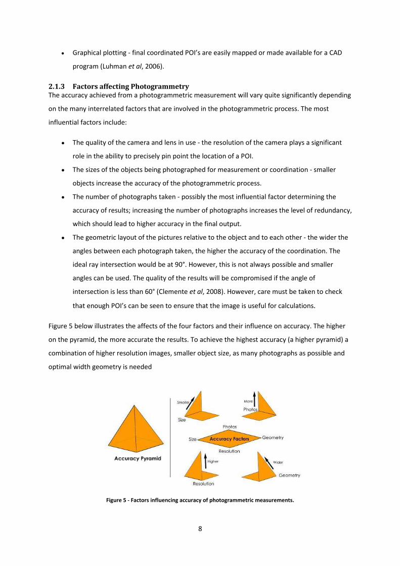
The accuracy achieved from a photogrammetric measurement will vary quite significantly depending
on the many interrelated factors that are involved in the photogrammetric process. The most
influential factors include:
• The quality of the camera and lens in use - the resolution of the camera plays a significant
role in the ability to precisely pin point the location of a POI.
• The sizes of the objects being photographed for measurement or coordination - smaller
objects increase the accuracy of the photogrammetric process.
• The number of photographs taken - possibly the most influential factor determining the
accuracy of results; increasing the number of photographs increases the level of redundancy,
which should lead to higher accuracy in the final output.
• The geometric layout of the pictures relative to the object and to each other - the wider the
angles between each photograph taken, the higher the accuracy of the coordination. The
ideal ray intersection would be at 90°. However, this is not always possible and smaller
angles can be used. The quality of the results will be compromised if the angle of
intersection is less than 60° (Clemente et al, 2008). However, care must be taken to check
that enough POI’s can be seen to ensure that the image is useful for calculations.
Figure 5 below illustrates the affects of the four factors and their influence on accuracy. The higher
on the pyramid, the more accurate the results. To achieve the highest accuracy (a higher pyramid) a
combination of higher resolution images, smaller object size, as many photographs as possible and
optimal width geometry is needed
Figure 5 - Factors influencing accuracy of photogrammetric measurements.
9
2.1.4 Scaling Photogrammetry
When an image is taken, the photogrammetric measurements essentially have no scale dimensions.
In order to scale objects in the image so it is possible to produce coordinates for a POI, it is necessary
that at least one known length measurement is visible in the image. If the actual coordinates of two
or more points in the image are known beforehand, this can be used to calculate the distances
between the two and hence give the image a scale. Another possibility for calculating the scale of an
image is to use a targeted fixture and measure along the object. The known distance between the
target marks can be used to scale the photographs. The most common form of scaling fixtures is
scale bars (Marshall, 1989).
Whenever possible, more than one distance should be used to scale the measurement as this
enables scale errors to be found. This is important because, when a single scale distance is used and
it is in error, the entire measurement will be incorrectly scaled. On the other hand, if multiple scale
distances are used, scale errors can be detected and removed. With two known distances, if one is in
error, a scale error can be detected, but it is usually not possible to determine which one is in error
(sometimes, however, it is possible to tell by inspecting the scale points). With three known scale
distances, it is usually possible to determine which is in error and remove it.
When scale bars are used, use of a bar that has more than two targets is an effective technique.
Alternatively, more than one scale bar can be used. A combination of both techniques can also be
used. Whenever feasible, it is recommended that multiple scale distances are used to maximise the
accuracies of the results. The scale distance(s) should be as long as practical because any inaccuracy
in the scale distance is magnified by the proportion of the size of the object to the scale distance
(Atkinson, 1996).
One disadvantage that is introduced by using a scale bar is the inability to include a vertical
direction. Using coordinated points instead of scale bars allows the introduction of heights,
orientation and azimuth.
2.2 FIG paper In 2010, at the 34th FIG conference in Sydney, Mr Gabriel Scarmana proposed an alternative concept
for mapping and navigating in GPS degraded areas. In such areas as dense forest or amongst high
rise buildings, GPS signals can be quite difficult to obtain or sometimes even impossible. Scarmana
(2010) proposed that an alternate method be employed where otherwise reliable GPS navigation
signals were blocked or weakened due to nearby high rise buildings or signal interference.
10
Scarmana’s proposal attempts to use close range photogrammetry to “survey city blocks where the
only sensory input is a single low-cost digital camera” (Scarmana, 2010). The process involves
traversing around a city block using a series of photographs taken from a simple off the shelf camera
and extracting 3D coordinates from visible POI’s in each photograph.
Scarmana’s main objective was to calculate and coordinate several important POI’s rather than
every visible one. Scarmana noted that he intended to combine his data with local and state
government authorities who “routinely carry out periodic surveys of public assets in order to update
and monitor their state” (Scarmana, 2010).
2.2.1 Location
Scarmana performed his experiment in narrow lanes sandwiched between high-rise buildings at
Surfers Paradise on the Gold Coast where “GPS signal paths provided limited visibility to satellites
and caused multipath effects, resulting in degraded navigation accuracy and reliability” (Scarmana,
2010).
In this project, the site used for recreating Scarmana’s project will be the UNSW campus, as it has
similar site characteristics. The final site selection was determined to be the Hut Dance studio in the
north-west corner of the UNSW Kensington Campus. Justifications for this site are outlined later in
Section 4.2.
2.2.2 Camera and Software
Scarmana used a Fuji A500 camera for his fieldwork. This is an off the shelf, readily available camera
with no special photogrammetric functions or lenses. It takes 5 megapixel photographs which is low
by today’s standard, and retailed for around $100 in 2008 (Scarmana, 2010). Scarmana theorised
that, if he could produce reasonable mapping and navigation results using a simple camera, then the
possibilities for using this technology as a navigation tool in the future would expand.
This investigation uses a more sophisticated camera than that used by Scarmana. A digital SLR Canon
450D camera with 12 megapixels, which retails for around $1200 (2010), was used in an attempt to
eliminate camera quality as a source of error or limitation. Section 3.1 outlines the camera in more
detail.
Scarmana’s processing and coordination of the photographs was done using Photomodeler Pro, a
photogrammetry program developed by EOS Systems. This low cost software is user friendly, has a
broad range of applications and is designed for use by non-photogrammetric experts. This program
was also used in this work in an attempt to maintain consistency between the two projects. More
information on Photomodeler can be found in Section 3.2.
11
2.2.3 Process
Measurements obtained from any photogrammetric processing cannot be fully accurate unless the
internal characteristics of the camera are known. Before any photogrammetric measurements are
made, the camera must be calibrated to “determine the optical and geometric characteristics of the
camera” (Scarmana, 2010). Scarmana used Photomodeler’s built-in calibration program to
determine the focal length and camera distortions. The process used by Photomodeler for the
calibration can be found in Section 3.3.
Scarmana’s proposed traverse length was a distance of approximately 450 m with “the plan to
measure a set of 80 POI’s (i.e. public assets such as traffic signs, bus shelters, street lights and major
trees) located along the streets” (Scarmana, 2010). Scarmana’s mapping/measuring project started
from three well defined control points. These three marks were established through the use of a
Leica TC2002 total station and consisted of “natural permanent targets such as the corner of tiles on
building walls or stable street signs” (Scarmana, 2010). The coordinates of the initial control points
were measured in GDA94 creating all future coordinate calculations in the same Datum. Scarmana
suggests that it was important that these three control points were spread apart at different
distances and did not lie on the same line. These control marks assisted initial orientation and scaling
of his project.
The first three images Scarmana took of his traverse were images of the “control points in
progression so as to bring forward along the street the correct scaling and orientation” (Scarmana,
2010). From then on images were taken every 10-15 metres as Scarmana moved forward around the
city loop. Scarmana was forced to use such short distances for long straights due to environmental
constraints. Scarmana suggests that, although not necessary, it is advantageous to use shorter
distances when entering a turn at street corners.
The geometry of the intersecting rays is a vital component of the processing if the images. It is
desirable to have the rays intersect at 90° and not at any angles less than 60° (Clemente et al,2008).
To improve angles, images may be taken in a zigzag pattern by alternating on different sides of the
road, as long as multiple POI’s are visible in at least two images. To ensure that enough POI’s were
recorded and no more field work would be required, Scarmana took an additional 20 more
photographs than was necessary.
To accurately connect sequential photographs together there must be sufficient suitable POI’s in
each image. A suitable POI must have a clearly defined edge or centre where the same point can be
confidently and accurately marked consistently on several different photographs. The best objects to
use as POI’s are edges of windows, road centrelines or the intersection of cracks in the footpath. If
12
an area has unsuitable POI’s there are several ways to overcome the problem. The ideal method is to
place temporary marks in the field of view of the camera; stick-on coded targets or more substantial
objects such as change plates can be used. The marks need not be coordinated but rather used for a
transfer of coordinates.
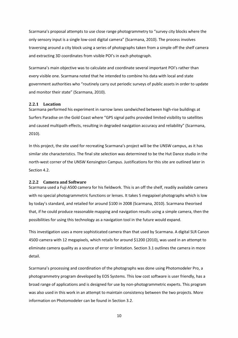
Figure 6 below shows an example of the trajectory of Scarmana’s camera as he took images in
progression. Photomodeler computes the 3D coordinates of the camera at each setup. It can be seen
that Scarmana used a zigzagging technique whilst taking his images.
The zigzagging technique is used when one photograph is taken from one side of the road in a
forward looking direction and then another photograph is taken from the other side of the road in
the same direction but a little further along in the direction of travel. This technique is the most
advantageous as it usually captures a larger array of POI’s. However care must be taken to maintain
suitable angles of intersection.
Figure 6 - Gabriel Scarmana's camera projections (Scarmana, 2010).
Scarmana loaded the images into Photomodeler and began marking all common visible POI’s.
Photomodeler has many useful tools to help mark images including a “sub-pixel marking tool”, which
is used to help determine the centroid of circular targets. Photomodeler suggests that these point
marking tools are accurate to around 1 pixel. 1 pixel equates to 5.1 μm on the image plane, 0.4 mm
at 2 m from the camera and 3 mm at 15 m from the camera.
The referencing stage is the final stage before the bundle adjustment is calculated. Common POI’s
were referenced in multiple photographs with at least six common POI’s being required to fully
reference an image. Once the minimum number of points has been referenced in at least two
images, automatic processing occurs. During this phase, Photomodeler “processes the camera
calibration and the referencing data and creates spatial point coordinates to produce 3D
coordinates” of all selected POI’s (Scarmana, 2010).

13
2.2.4 Results
Over the 450 metres travelled, Scarmana’s final coordinate errors were ±3m or 1:150m. An example
of the errors can be seen below in Figure 7.
Figure 7 - Results obtained by Scarmana (Scarmana, 2010).
The above graph shows that positional accuracy degraded with distance travelled. Scarmana
suggests that positional errors are directly dependent upon on (Scarmana, 2010):
• Distance covered
• Number of observation or camera stations
• Precision of the system components
• Measuring geometry
The distance covered in this thesis will be significantly shorter with a distance of 140 metres
travelled. Based on Scarmana’s results this project should produce results to within one metre
accuracies. However this project is using a far superior camera so it would be expected that the
accuracies would be increased even further.
2.3 Camera Calibration Instrument calibration is an important element in all surveying fields including close range
photogrammetry. Camera calibration has multiple functions for close range photogrammetry as it
accurately evaluates several functions of the camera that can affect image calculation and
coordination. Apart from evaluating both the performance and stability of the cameras lens, an
accurate calibration can also determine the optical and geometrical parameters of the lens, camera
system and image data acquisition system.
Photomodeler has an inbuilt calibration program that is simple to run and records and stores all
parameters for that camera for all its future calculations. The parameters that are solved for by the
program include:
• Principal Distance or Focal Length
14
• Principal Points
• Format Width/Height
• Radial Distortions
• Decentring Distortions
Along with the general calibration that is performed before the commencement of field work there
is also the option to perform an infield calibration which will produce a more accurate set of results
since it is possible to calibrate the camera using objects of similar size.
The calibration results can be seen later in this thesis in Section 3.3.
2.4 Camera Parameters
2.4.1 Principal Distance or Focal Length
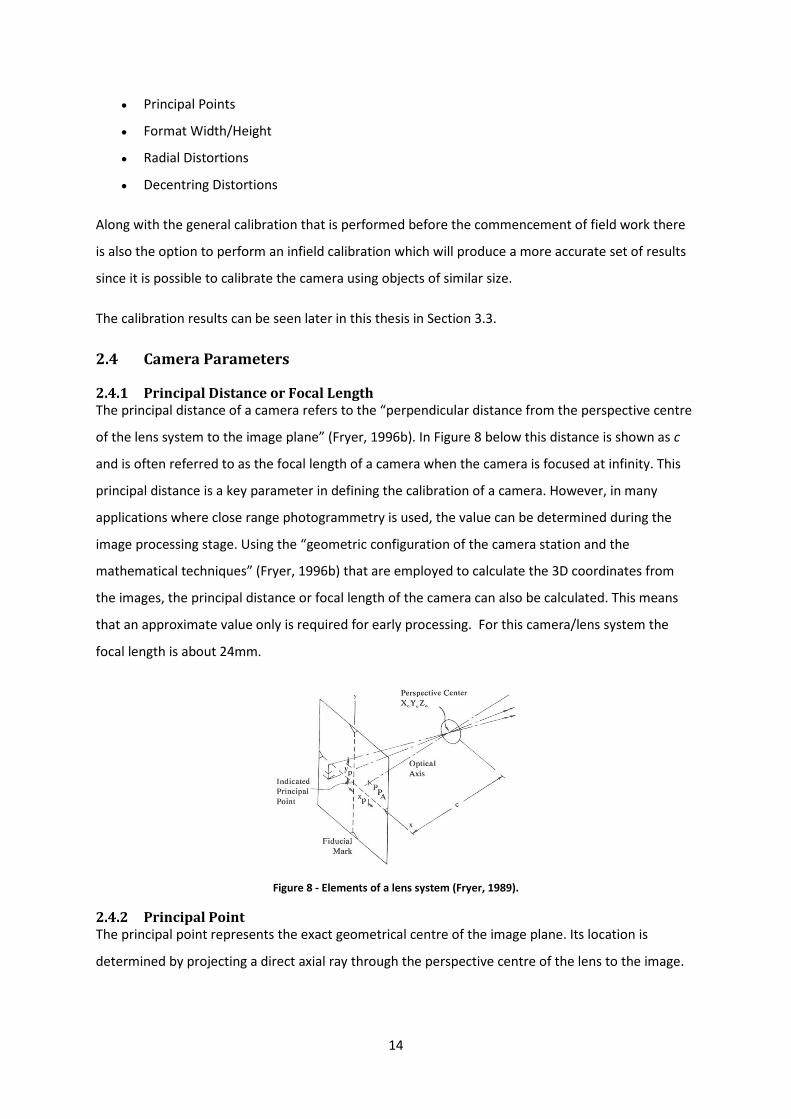
The principal distance of a camera refers to the “perpendicular distance from the perspective centre
of the lens system to the image plane” (Fryer, 1996b). In Figure 8 below this distance is shown as c
and is often referred to as the focal length of a camera when the camera is focused at infinity. This
principal distance is a key parameter in defining the calibration of a camera. However, in many
applications where close range photogrammetry is used, the value can be determined during the
image processing stage. Using the “geometric configuration of the camera station and the
mathematical techniques” (Fryer, 1996b) that are employed to calculate the 3D coordinates from
the images, the principal distance or focal length of the camera can also be calculated. This means
that an approximate value only is required for early processing. For this camera/lens system the
focal length is about 24mm.
Figure 8 - Elements of a lens system (Fryer, 1989).
2.4.2 Principal Point
The principal point represents the exact geometrical centre of the image plane. Its location is
determined by projecting a direct axial ray through the perspective centre of the lens to the image.
2.4.3 Indicated Principal Point
In modern digital cameras the fiducial origin is now referred to as the indicated principal
point refers to the point on the image plane that the processing software determines to be the ideal
position for the origin. In an ideal camera with no distortions the indicated principal point would
correspond with the principal point. Howeve
Therefore, to centre the image coordinates correctly, it is necessary to add calculated offsets (
Yp) from the principal point to the origin of the principal point coordinate system. The origin
principal point coordinate system will vary depending on software used.
The offset between the principal point and indicated principal point
less than 1mm. Section 3.3 shows the calculated difference between the princip
principal point for this thesis.
2.4.4 Radial Distortions - K
The radial distortion component of the calibration is the determination of any
the image rays from the principal point, i.e. closer to or further away from the principal point.
amount of distortion increases with
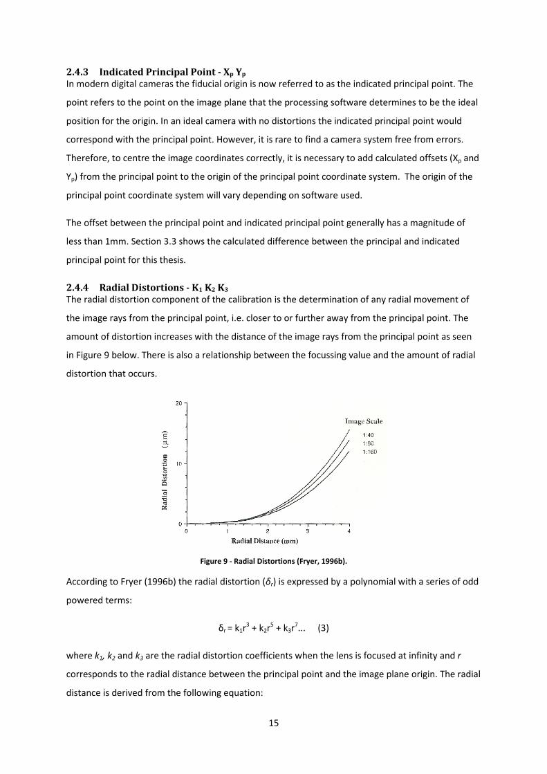
in Figure 9 below. There is also a relatio
distortion that occurs.
According to Fryer (1996b) the radial distortion (
powered terms:
where k1, k2 and k3 are the radial distortion coefficients when the lens is focused at infinity and
corresponds to the radial distance between the principal point and the image plane origin. The radial
distance is derived from the following equation:
15
Indicated Principal Point - Xp Yp
In modern digital cameras the fiducial origin is now referred to as the indicated principal
point refers to the point on the image plane that the processing software determines to be the ideal
for the origin. In an ideal camera with no distortions the indicated principal point would
correspond with the principal point. However, it is rare to find a camera system free from errors.
Therefore, to centre the image coordinates correctly, it is necessary to add calculated offsets (
from the principal point to the origin of the principal point coordinate system. The origin
principal point coordinate system will vary depending on software used.
The offset between the principal point and indicated principal point generally ha
shows the calculated difference between the principal and indicated
K1 K2 K3
The radial distortion component of the calibration is the determination of any radial
the image rays from the principal point, i.e. closer to or further away from the principal point.
amount of distortion increases with the distance of the image rays from the principal point
below. There is also a relationship between the focussing value and the amount of radial
Figure 9 - Radial Distortions (Fryer, 1996b).
) the radial distortion (δr) is expressed by a polynomial with a series of
δr = k1r3 + k2r
5 + k3r7... (3)
are the radial distortion coefficients when the lens is focused at infinity and
corresponds to the radial distance between the principal point and the image plane origin. The radial
distance is derived from the following equation:
In modern digital cameras the fiducial origin is now referred to as the indicated principal point. The
point refers to the point on the image plane that the processing software determines to be the ideal
for the origin. In an ideal camera with no distortions the indicated principal point would
a camera system free from errors.
Therefore, to centre the image coordinates correctly, it is necessary to add calculated offsets (Xp and
from the principal point to the origin of the principal point coordinate system. The origin of the
generally has a magnitude of
al and indicated
radial movement of
the image rays from the principal point, i.e. closer to or further away from the principal point. The
the distance of the image rays from the principal point as seen
nship between the focussing value and the amount of radial
) is expressed by a polynomial with a series of odd
are the radial distortion coefficients when the lens is focused at infinity and r
corresponds to the radial distance between the principal point and the image plane origin. The radial
Values for the radial distortions of the camera used in this thesis can be found in
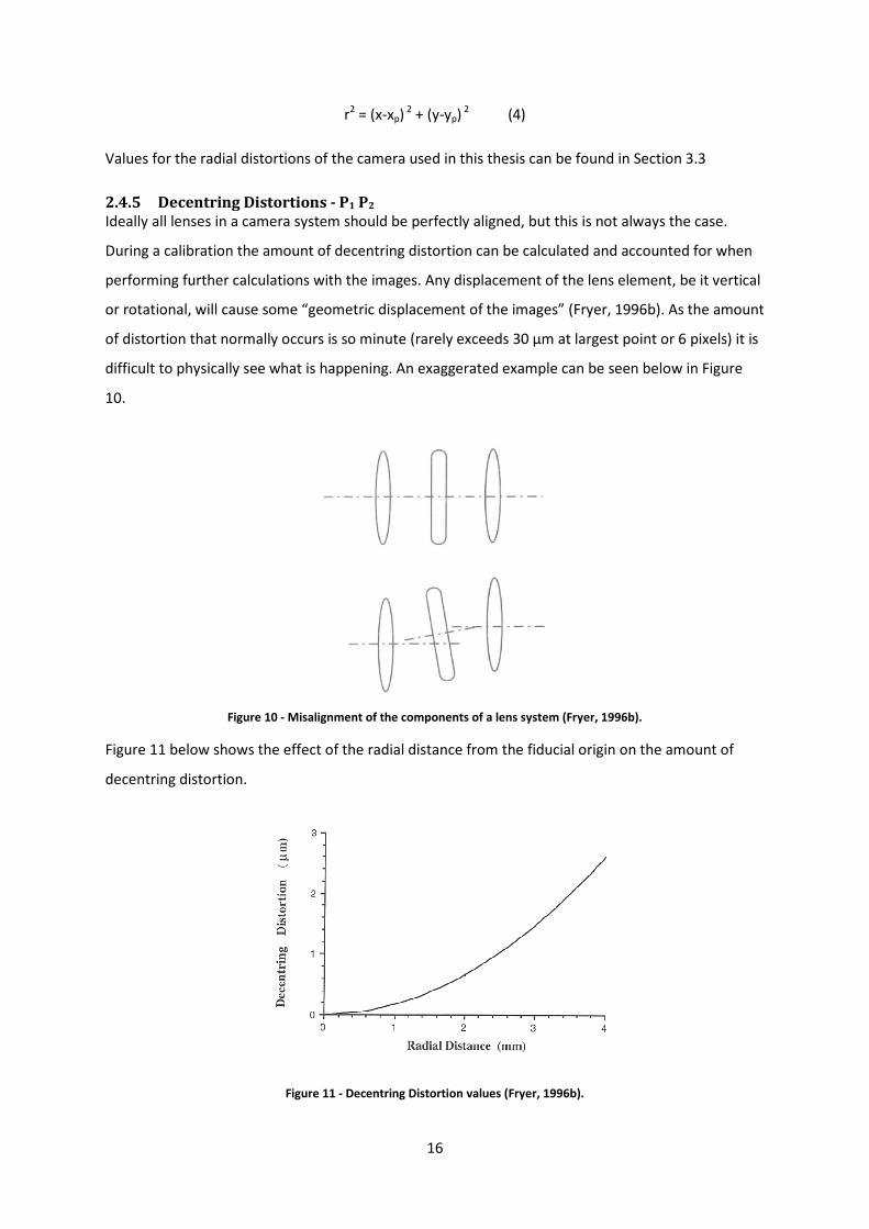
2.4.5 Decentring Distortions
Ideally all lenses in a camera system should be perfectly aligned
During a calibration the amount of decentring distortion can be calculated and accounted for when
performing further calculations with the images. Any displacement of the lens
or rotational, will cause some “geometric displacement of the images” (Fryer, 1
of distortion that normally occurs is so minute (rarely exceeds 30
difficult to physically see what is happening. A
10.
Figure 10 - Misalignment of the components of a lens system (Fryer, 1996
Figure 11 below shows the effect of the radial distance from the fiducial origin on the amount of
decentring distortion.
Figure
16
r2 = (x-xp) 2 + (y-yp) 2 (4)
Values for the radial distortions of the camera used in this thesis can be found in
Decentring Distortions - P1 P2
Ideally all lenses in a camera system should be perfectly aligned, but this is not always the case.
e amount of decentring distortion can be calculated and accounted for when
performing further calculations with the images. Any displacement of the lens element
or rotational, will cause some “geometric displacement of the images” (Fryer, 1996
of distortion that normally occurs is so minute (rarely exceeds 30 μm at largest point or 6 pixels)
difficult to physically see what is happening. An exaggerated example can be seen below in
Misalignment of the components of a lens system (Fryer, 1996b
below shows the effect of the radial distance from the fiducial origin on the amount of
Figure 11 - Decentring Distortion values (Fryer, 1996b).
Values for the radial distortions of the camera used in this thesis can be found in Section 3.3
but this is not always the case.
e amount of decentring distortion can be calculated and accounted for when
element, be it vertical
996b). As the amount
m at largest point or 6 pixels) it is
n exaggerated example can be seen below in Figure
b).
below shows the effect of the radial distance from the fiducial origin on the amount of

17
According to Fryer (1996b) the above distortion is modelled on the following equation, where P(r)
refers to the amount of decentring distortion that occurs:
���� � �� ��� � ���� (5)
P1 and P2 refer to values when the camera is focused at infinity and r is the radial distance between
the principal point and the fiducial origin.
Values for the decentring distortions of the camera used in this thesis can be found in Section 3.3.
18
3. Camera Calibration
3.1 Project Camera The camera used for this thesis project was the 12 megapixel Canon EOS 450D (s/n Camera body:
3080700873, Lens: 116369, Camera Number: 4). Prior to beginning field work it was essential that
the user became familiar with the different modes, settings and functions of the camera. A full list
of the cameras specifications can be found in appendix 8.1.
• Type - the Canon EOS is a non-metric camera meaning it usually is cheaper than a metric
camera, has interchangeable lenses, is lighter in weight and is smaller. However, non-metric
cameras have an unstable interior orientation. The effective focal length may change for
each exposure and the direction of the optical axis may alter with focusing movement.
• Settings - after several experiments it was determined that the best setting for the camera is
the “M”, or manual setting. On this setting both the shutter speed and aperture values can
be set to the appropriate values. When outside there is no particular combination of settings
that will be appropriate for all photographs.
• Extras - when taking images, particularly for the calibrations, a tripod should be used for
stability. A cable release and eye piece should also be used to increase the accuracy of the
calibration.
• Save format - images are saved in JPEG format. This is the only format that must be saved, as
Photomodeler does not require the RAW data for its processing. Raw image files are
sometimes called digital negatives, as they fulfil the same role as negatives in film
photography.
The camera used is the single largest distinguishing factor when it comes to the quality of the results
obtained. Photographs of high resolution with appropriate exposure allow for referenced marks to
be precisely marked in all photographs. With the manual mode you have full control over every
aspect of your camera. You are able to set the aperture, shutter speed, ISO, white balance, and flash
values. A display in the viewfinder reports whether the camera thinks your settings will result in
under, over, or correctly exposed photos.
3.1.1 Camera Calculations
In addition to understanding the functions and settings of the camera to be used in the survey, it
was necessary to calculate several internal measurements of the camera, including FOV, pixel size
and view angles. Calculations can be found in detail in Appendix 8.2 and 8.3
Camera Settings for Calculations
Vertical Camera Height: 1.395 m
19
Wall to Camera Distance: 2.01m
Camera Shooting Mode: Manual
Shutter Speed: 1/125
Aperture: 8.0
ISO: 400
Image Quality: L
Note: The camera settings were kept constant for the entirety of the exercise
3.1.2 Field Of View Calculation
Field of view (FOV) is an important parameter as it is necessary to capture everything that is seen in
the viewfinder in the image. Simple field exercises were performed to determine whether the
extents seen in the view finder were identical to the extents produced in the photograph. The
experiment consisted of measuring the distance visible through the view finder on a wall both
vertically and horizontally and comparing the measurements to a photograph taken with a scale bar
(level staff) in the image for an accurate measurement of the photograph distance. It was also useful
to know the FOV angles for planning close range photogrammetry surveys.
Horizontal
View Finder: 1.698 m Photograph: 1.741 m
Therefore, at 2.01m the photograph will capture 43mm more of the image horizontally than is seen
in the view finder (≈21.5mm to the left and right of the image).
Vertical
View Finder: 1.107 m Photograph: 1.155 m
Therefore, at 2.01m the photograph will capture 48mm more of the image vertically than is seen in
the view finder (≈24 mm to the top and bottom of the image).
From the above calculations, it can be said that when a photograph is taken more of the image will
be captured in the photograph than is seen in the view finder.
Given that the extra image area taken in the photograph in both the horizontal and vertical
directions differ by 5 mm it can be assumed that there is an equal amount of extra image taken on
all four sides, i.e. ≈ 23 mm for an image taken at 2.01 m from the object. The discrepancy would
have been due to the facts that level staffs were used as the scale bar and that human error is
entered into the calculations when estimating the millimetres between intervals.
20
3.1.3 Pixel Size Calculation
Pixel, or Picture Element, is defined in the Oxford Dictionary online edition, as “a minute area of
illumination on a display screen, one of many from which an image is composed” (Oxford, 2011). All
electronic displays consist of thousands of illuminated pixels that, when lined together, form an
image or display.
From the previous calculations, both the horizontal and vertical distances of the photograph have
already been determined. Using this information it was possible to calculate the size of each pixel as
well as determining if they are square or rectangular.
Horizontal
Distance: 1.741 m No of Pixels: 4272
Therefore there are 2.454 pixels per millimetre horizontally
Vertical
Distance: 1.155 m No of Pixels: 2848
Therefore there are 2.466 pixels per millimetre vertically
It is reasonable to assume that each pixel is square. The slight discrepancy in the number of pixels
per millimetre would again be due to the human error introduced in estimating the distances whilst
using the level staff.
If each pixel is assumed to be square, then there are 2.46 pixels per millimetre or each pixel is ≈
0.41mm x 0.41 mm at a distance of 2.01 m. This equates to 5.1 μm square on the image plane.
3.1.4 View Angle Calculation
Knowing the view angle of a camera makes it possible to calculate the distance from the object that
is required in order to fully capture the required parts of the object in a photograph.
Using the values from the previous calculations the following viewing angles were determined:
Horizontal - The horizontal view angle is 46° 50’
The 46° 50’ horizontal view angle that is produced in the photograph is similar to that of the human
eye which has a viewing angle of about 45°.
Vertical - The vertical view angle is 32° 04’
The calculations show that, when photographing an image, the field of view extends approximately
45° from the origin horizontally and approximately 30° vertically from the origin. If the size of the
21
object to be captured is known, these values can be used to position the camera at the correct
distance to capture the entire object in the photograph. An object three metres tall would require a
distance of 5.2m in order to capture the whole image.
Knowing the viewing angle also indicates where the camera should be placed to achieve a good
overlap of photographs. It should be noted that the calculations were also performed for the values
obtained from the view finder. As expected, the view angles were slightly less than the angles
produced in the photograph.
3.2 Photomodeler Pro The program used for the majority of this project was Photomodeler Pro 6 which is a Windows
based photogrammetry software program that provides “image-based modelling, for accurate
measurement and 3D models in engineering, architecture, film and forensics” (EOS Systems, 2011).
Photomodeler takes 2D photograph images and creates a 3D representation of the image complete
with 3D coordinates.
An advantage of Photomodeler is that it is designed in such a way that the user need not be an
expert in the photogrammetry field. Photomodeler was used in this project to maintain consistency
with Scarmana’s experiments and results.
As Photomodeler is designed for non-photogrammetry experts, the website provides several
interactive tutorials designed to instruct the user on the basics of the program. Relevant tutorials
were completed prior to using the software. The tutorials covered the basics of Photomodeler
including:
• Calibration, both single sheet as well as in field calibration
• Point projection
• Dimensioning
• Measuring
• Referencing
• Automated Coded Targets
Figure 12 - Referencing Tutorial in Photomodeler (EOS Systems, 2011).
22
3.3 Calibration Initial practical work focussed on calibration and analysis of the Canon EOS 450D camera. As
mentioned in Section 2.3, many different distortions can occur in the internal geometry of a camera
that will affect the overall accuracy of the measurements. For this project the camera has been
calibrated three times, twice with Photomodeler and once with iWitness. The calibration was carried
out twice with Photomodeler to analyse consistency with the results and distortions and once with
iWitness to compare results using different software.
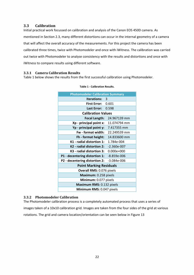
3.3.1 Camera Calibration Results
Table 1 below shows the results from the first successful calibration using Photomodeler.
Table 1 - Calibration Results.
Photomodeler Calibration Summary
Iterations: 3
First Error: 0.601
Last Error: 0.598
Calibration Values
Focal Length: 24.967139 mm
Xp - principal point x: 11.074794 mm
Yp - principal point y: 7.417355 mm
Fw - format width: 22.249539 mm
Fh - format height: 14.833600 mm
K1 - radial distortion 1: 1.784e-004
K2 - radial distortion 2: -2.360e-007
K3 - radial distortion 3: 0.000e+000
P1 - decentering distortion 1: -8.859e-006
P2 - decentering distortion 2: -3.084e-006
Point Marking Residuals
Overall RMS: 0.076 pixels
Maximum: 0.258 pixels
Minimum: 0.077 pixels
Maximum RMS: 0.132 pixels
Minimum RMS: 0.047 pixels
3.3.2 Photomodeler Calibration
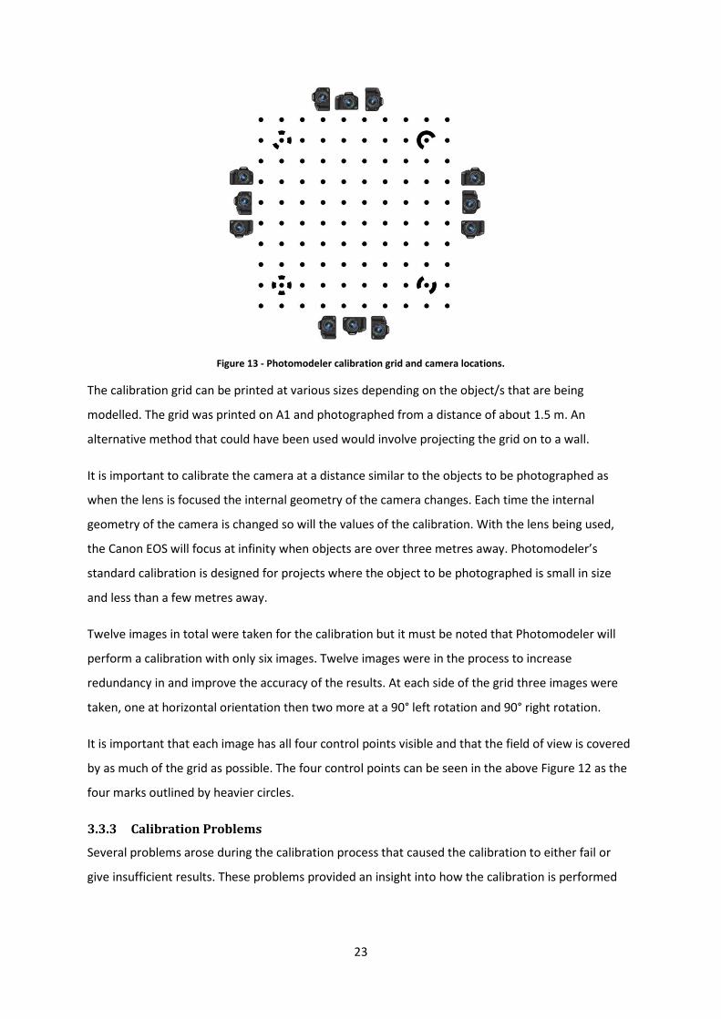
The Photomodeler calibration process is a completely automated process that uses a series of
images taken of a 10x10 calibration grid. Images are taken from the four sides of the grid at various
rotations. The grid and camera location/orientation can be seen below in Figure 13
23
Figure 13 - Photomodeler calibration grid and camera locations.
The calibration grid can be printed at various sizes depending on the object/s that are being
modelled. The grid was printed on A1 and photographed from a distance of about 1.5 m. An
alternative method that could have been used would involve projecting the grid on to a wall.
It is important to calibrate the camera at a distance similar to the objects to be photographed as
when the lens is focused the internal geometry of the camera changes. Each time the internal
geometry of the camera is changed so will the values of the calibration. With the lens being used,
the Canon EOS will focus at infinity when objects are over three metres away. Photomodeler’s
standard calibration is designed for projects where the object to be photographed is small in size
and less than a few metres away.
Twelve images in total were taken for the calibration but it must be noted that Photomodeler will
perform a calibration with only six images. Twelve images were in the process to increase
redundancy in and improve the accuracy of the results. At each side of the grid three images were
taken, one at horizontal orientation then two more at a 90° left rotation and 90° right rotation.
It is important that each image has all four control points visible and that the field of view is covered
by as much of the grid as possible. The four control points can be seen in the above Figure 12 as the
four marks outlined by heavier circles.
3.3.3 Calibration Problems
Several problems arose during the calibration process that caused the calibration to either fail or
give insufficient results. These problems provided an insight into how the calibration is performed
24
and what factors are the most influential when taking the photographs. The major problems
consisted of:
• Background error - the first calibration attempt took place in the corridor of the top level of
the Electrical Engineering Building. The surface of the floor consists of black and white
speckled linoleum and the room is lit with florescent bulbs. The image acquisition was
completed with relative ease but problems were encountered during the initial processing of
the images. Photomodeler was picking up sections of the floor around the calibration sheet
and using them as reference points to perform the calibration. This caused errors to be
greatly exaggerated and the calibration to fail. An unsuccessful attempt was made to
manually remove these unwanted marks from the calibration.
• Glossy cover - the second problem that occurred during the calibration process was an error
with Photomodeler recognising the dots on the grid. The program provided the following
advice on resolving this issue:
“A large percentage of your points are sub-pixel marked so it is assumed you are
striving for a high accuracy result. The largest residual (Point49 - 2.46) is greater
than 1.00 pixels.
Suggestion: In high accuracy projects, strive to get all point residuals under
1.00 pixels. If you have just a few high residual points, study them on each photo to
ensure they are marked and referenced correctly. If many of your points have high
residuals then make sure the camera stations are solving correctly. Ensure that you
are using the best calibrated camera possible. Remove points that have been
manually marked unless you need them.”
It was originally thought that this error was due to light reflections on the grid. An attempt
was made to evenly light the whole grid with transportable photography lamps, but this had
little to no effect. It was then suggested that the fact that the grid was printed on glossy
paper might be having an effect. After re-printing the grid on matt paper, the above error no
longer appeared.
• Image coverage - The calibration grid should cover at least 80% of the combined image
format. It is not essential that each individual image has 80% coverage. Less than 80%
coverage will result in less accurate calibration.
25
3.3.4 Image Acquisition
To ensure camera and image stability a tripod and remote trigger were used for image acquisition.
The focus was set for the first image then unchanged for the remainder of the photographs
(although it was checked each time before taking an image). The grid was taped to the floor and
weights were placed on corners and edges for extra stability.
When taking the photographs, the camera was set to TV setting which allows for the shutter speed
to be manually set and the aperture automatically set accordingly. This setting was used following
experimentation with the differences between setting either the shutter speed or aperture manually
as well as setting both manually. It was found that the best setting for taking images in this light was
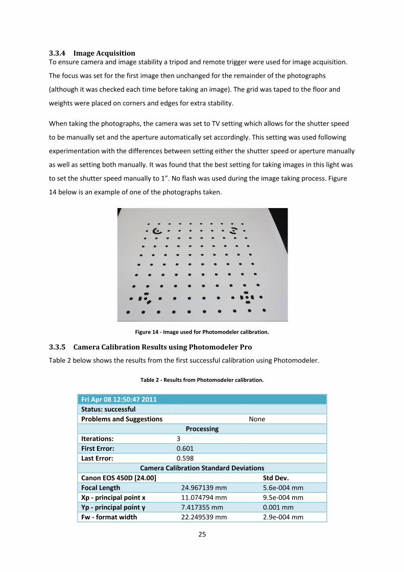
to set the shutter speed manually to 1”. No flash was used during the image taking process. Figure
14 below is an example of one of the photographs taken.
Figure 14 - Image used for Photomodeler calibration.
3.3.5 Camera Calibration Results using Photomodeler Pro
Table 2 below shows the results from the first successful calibration using Photomodeler.
Table 2 - Results from Photomodeler calibration.
Fri Apr 08 12:50:47 2011
Status: successful
Problems and Suggestions None
Processing
Iterations: 3
First Error: 0.601
Last Error: 0.598
Camera Calibration Standard Deviations
Canon EOS 450D [24.00] Std Dev.
Focal Length 24.967139 mm 5.6e-004 mm
Xp - principal point x 11.074794 mm 9.5e-004 mm
Yp - principal point y 7.417355 mm 0.001 mm
Fw - format width 22.249539 mm 2.9e-004 mm
26
Fh - format height Value: 14.833600 mm
K1 - radial distortion 1 1.784e-004 2.9e-007
K2 - radial distortion 2 -2.360e-007 2.4e-009
K3 - radial distortion 3 0.000e+000
P1 - decentering distortion 1 -8.859e-006 5.1e-007
P2 - decentering distortion 2 -3.084e-006 5.4e-007
Photograph Quality
Total Number: 12 Bad Photos: 0 Weak Photos: 0 OK Photos: 12
Average Photo Point Coverage: 87%
Point Marking Residuals
Overall RMS: 0.076 pixels
Maximum: 0.258 pixels Point 19 on Photo 5
Minimum: 0.077 pixels Point 60 on Photo 6
Maximum RMS: 0.132 pixels Point 3
Minimum RMS: 0.047 pixels Point 43
If the calibration is to be acceptable and useable for a project, then the value of the “Last Error”
should be less than 1. The last error value for this calibration (0.598) is acceptable (<1), thus the
calibration was successful and stored for use. Photomodeler cannot solve for both the “Format
Width” and the “Format Height”. The “Format Width” refers to the total width of the image format
or image plane.
The principal point and indicated principal points should always be less than 1 mm apart, in this case
they were calculated as x=5.5x10⁻⁴ mm and y=0.05 mm.
“Radial Distortion 3” was not calculated as it is only required when wide angle lenses are used. For
an acceptable outcome, the “Maximum Residual” value should be no greater than 1.5 pixels and be
under 1 pixel for a high accuracy; in this case the MR was 0.258, indicating a high accuracy
calibration.
The “Maximum RMS” for this calibration was 0.132 pixels on point 3. This value is well below the
suggested value 0.5 pixels which is a maximum required for an accurate calibration.
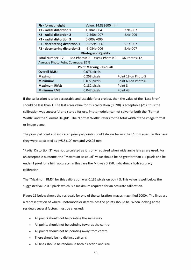
Figure 15 below shows the residuals for one of the calibration images magnified 2000x. The lines are
a representation of where Photomodeler determines the points should be. When looking at the
residuals several factors must be checked:
• All points should not be pointing the same way
• All points should not be pointing towards the centre
• All points should not be pointing away from centre
• There should be no distinct patterns
• All lines should be random in both direction and size
27
By viewing these factors it is possible determine whether the calibration contains systematic errors.
If the residual lines are completely random then it is likely that the only errors present are random
errors that can be ignored. If a distinct pattern is found then further investigation must be
completed as there are most likely systematic errors involved in the calibration process. Systematic
errors may have been caused by bad lighting in one area of the calibration grid or a slight movement
of the grid between photographs.
Figure 15 - Residuals produced by Photomodeler calibration.
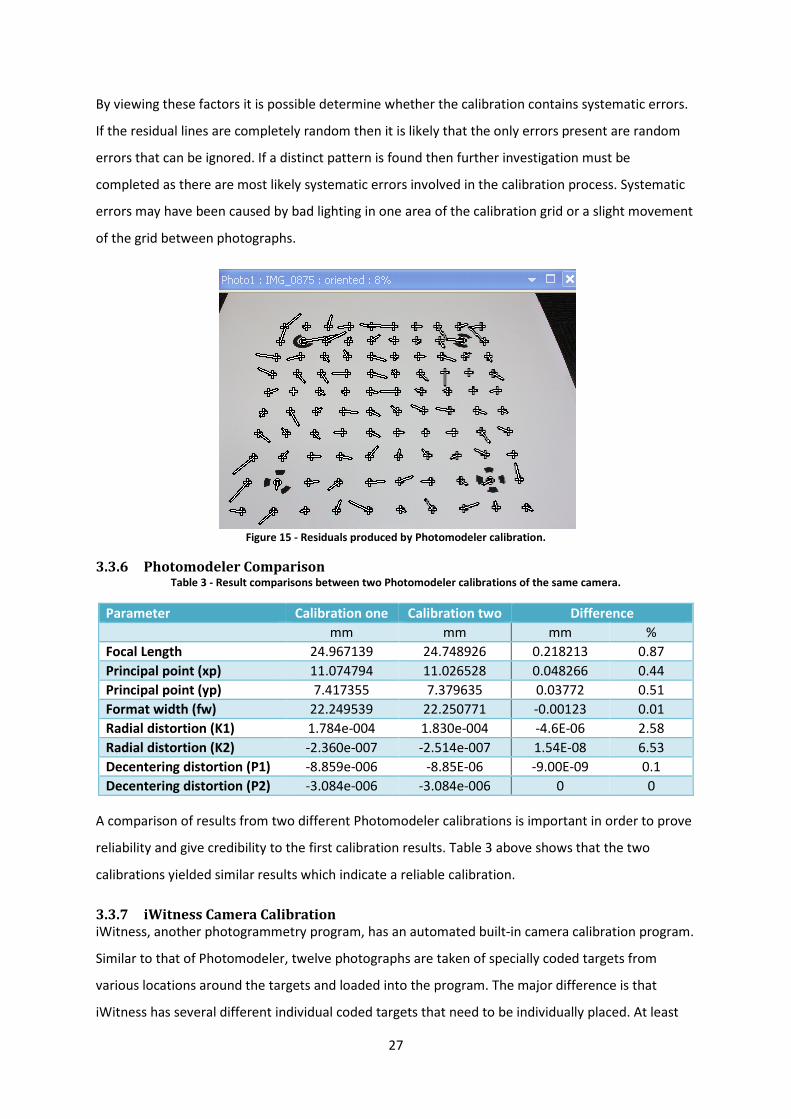
3.3.6 Photomodeler Comparison Table 3 - Result comparisons between two Photomodeler calibrations of the same camera.
Parameter Calibration one Calibration two Difference
mm mm mm %
Focal Length 24.967139 24.748926 0.218213 0.87
Principal point (xp) 11.074794 11.026528 0.048266 0.44
Principal point (yp) 7.417355 7.379635 0.03772 0.51
Format width (fw) 22.249539 22.250771 -0.00123 0.01
Radial distortion (K1) 1.784e-004 1.830e-004 -4.6E-06 2.58
Radial distortion (K2) -2.360e-007 -2.514e-007 1.54E-08 6.53
Decentering distortion (P1) -8.859e-006 -8.85E-06 -9.00E-09 0.1
Decentering distortion (P2) -3.084e-006 -3.084e-006 0 0
A comparison of results from two different Photomodeler calibrations is important in order to prove
reliability and give credibility to the first calibration results. Table 3 above shows that the two
calibrations yielded similar results which indicate a reliable calibration.
3.3.7 iWitness Camera Calibration
iWitness, another photogrammetry program, has an automated built-in camera calibration program.
Similar to that of Photomodeler, twelve photographs are taken of specially coded targets from
various locations around the targets and loaded into the program. The major difference is that
iWitness has several different individual coded targets that need to be individually placed. At least
28
thirteen targets must be used and one or more must be at a different height to the others. The
layout used for the calibration in this investigation can be seen in Figure 16 below.
Figure 16 - Coded targets and layout for iWitness calibration.
Seventeen images were taken in an effort to maximise the image quality of the photographs taken
and loaded into the iWitness program. One notable advantage of this program is that calibration
takes about 2 min to perform, as compared to 15 minutes with the Photomodeler program. This is a
consideration to be examined when selecting the processing software.
Another consideration is the fact that iWitness is less dependent on the location of the camera when
taking the photographs. Whereas Photomodeler has very specific locations required for the image
acquisition, the photographs can be taken from any position around the targets for iWitness. The
iWitness calibration was done with the camera positioned 1.5 m from the coded targets.
iWitness has an option to print larger targets for the calibration process which allows the camera to
be calibrated at a longer distance.
3.3.8 iWitness Results and Comparisons
Table 4 below compares the results obtained from the iWitness calibration with the Photomodeler
results.
Table 4 - Results from calibration of the same camera using iWitness and Photomodeler.
Parameter iWitness Photomodeler Difference
mm mm mm %
Focal Length 23.727 24.967 1.240 5.23
Principal point (xp) -0.071 11.074 11.145 -
Principal point (yp) 0.040 7.417 7.377 -
Radial distortion (K1) 1.979e-004 1.784e-004 1.95E-05 9.85
Radial distortion (K2) -3.457e-007 -2.360e-007 -1.10E-07 31.82
Decentering distortion (P1) -1.115e-005 -8.859e-006 -2.29E-06 20.54
Decentering distortion (P2) -2.909e-006 -3.084e-006 1.75E-07 6.02
29
The first major comparison made between the two calibration results was the difference between
focal lengths. The value given to the focal length is in direct proportion with the length of the lens
when focused for the image acquisition. The difference of over 1mm in focal length was expected
due to the fact that the calibrations were performed at different times, and thus the camera was
refocussed (changing focal length).
The second major difference in the calibration comparisons was the difference in principal point
locations. This is because although both Photomodeler and iWitness use the same reference frame
they clearly use a different location for the origin of their principal point coordinate system. From
the x and y principal point values it was determined that Photomodeler uses the bottom left corner
of its image for the origin of its principal point coordinate system whilst iWitness uses a point closer
to the geometrical centre of the photographs.
30
4. Field work The field work component of this thesis was carried out over four days during August and
September. The majority of the photographs were taken on August 10th but after an initial
processing attempt it was discovered that more photographs were required to complete a loop.
Three more field days were completed on the 22nd of August and the 7th and 13th of September
2011.
4.1 Trial
Before the commencement of field work a trial was completed to determine what factors need to be
considered during the field work to achieve maximum accuracy. A simple straight line of the
walkway at UNSW was used as the test area due to being able to use the intersections of the pavers
as POI’s to reference in photographs. The site chosen can be seen in Figure 17.
Figure 17 - Trial site.
The trial was invaluable in helping to understand how Photomodeler works and the importance of
referencing corresponding points correctly. One incorrectly referenced point will cause large
positional errors in the job and Photomodeler will be unsuccessful in its attempt to process the
photographs. It became clear that it can be easy to miss reference points in areas where there are
similar looking POI’s i.e. the joints of pavers on a path. In an attempt to avoid this care was taken
when in the field to select distinguishable POI’s when possible.
When doing some brief processing in Photomodeler it was discovered that each photograph in the
project has three different options for the processing. “Use and adjust”, “Use and don’t adjust” and
“Do not use”. This became useful when the incomplete loop was processed. If the project is
processed and a photograph is unsuccessfully orientated Photomodeler will automatically change
that photographs setting to “Do not use” and it must be manually changed back to “Use and adjust”
before the project is reprocessed.
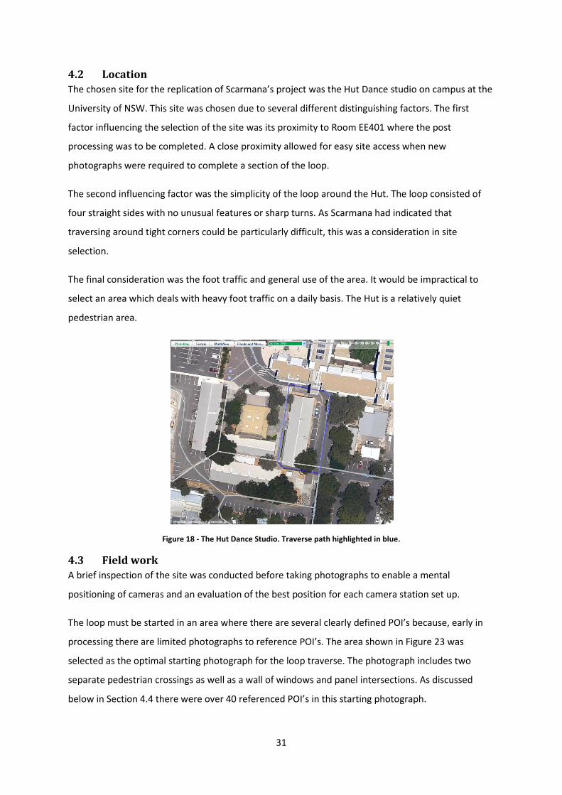
31
4.2 Location
The chosen site for the replication of Scarmana’s project was the Hut Dance studio on campus at the
University of NSW. This site was chosen due to several different distinguishing factors. The first
factor influencing the selection of the site was its proximity to Room EE401 where the post
processing was to be completed. A close proximity allowed for easy site access when new
photographs were required to complete a section of the loop.
The second influencing factor was the simplicity of the loop around the Hut. The loop consisted of
four straight sides with no unusual features or sharp turns. As Scarmana had indicated that
traversing around tight corners could be particularly difficult, this was a consideration in site
selection.
The final consideration was the foot traffic and general use of the area. It would be impractical to
select an area which deals with heavy foot traffic on a daily basis. The Hut is a relatively quiet
pedestrian area.
Figure 18 - The Hut Dance Studio. Traverse path highlighted in blue.
4.3 Field work
A brief inspection of the site was conducted before taking photographs to enable a mental
positioning of cameras and an evaluation of the best position for each camera station set up.
The loop must be started in an area where there are several clearly defined POI’s because, early in
processing there are limited photographs to reference POI’s. The area shown in Figure 23 was
selected as the optimal starting photograph for the loop traverse. The photograph includes two
separate pedestrian crossings as well as a wall of windows and panel intersections. As discussed
below in Section 4.4 there were over 40 referenced POI’s in this starting photograph.
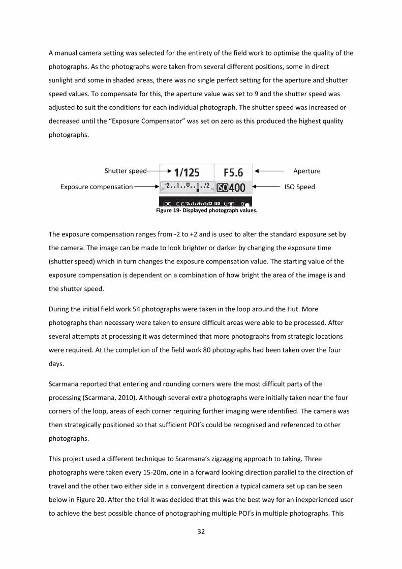
32
A manual camera setting was selected for the entirety of the field work to optimise the quality of the
photographs. As the photographs were taken from several different positions, some in direct
sunlight and some in shaded areas, there was no single perfect setting for the aperture and shutter
speed values. To compensate for this, the aperture value was set to 9 and the shutter speed was
adjusted to suit the conditions for each individual photograph. The shutter speed was increased or
decreased until the “Exposure Compensator” was set on zero as this produced the highest quality
photographs.
Shutter speed Aperture
Exposure compensation ISO Speed
The exposure compensation ranges from -2 to +2 and is used to alter the standard exposure set by
the camera. The image can be made to look brighter or darker by changing the exposure time
(shutter speed) which in turn changes the exposure compensation value. The starting value of the
exposure compensation is dependent on a combination of how bright the area of the image is and
the shutter speed.
During the initial field work 54 photographs were taken in the loop around the Hut. More
photographs than necessary were taken to ensure difficult areas were able to be processed. After
several attempts at processing it was determined that more photographs from strategic locations
were required. At the completion of the field work 80 photographs had been taken over the four
days.
Scarmana reported that entering and rounding corners were the most difficult parts of the
processing (Scarmana, 2010). Although several extra photographs were initially taken near the four
corners of the loop, areas of each corner requiring further imaging were identified. The camera was
then strategically positioned so that sufficient POI’s could be recognised and referenced to other
photographs.
This project used a different technique to Scarmana’s zigzagging approach to taking. Three
photographs were taken every 15-20m, one in a forward looking direction parallel to the direction of
travel and the other two either side in a convergent direction a typical camera set up can be seen
below in Figure 20. After the trial it was decided that this was the best way for an inexperienced user
to achieve the best possible chance of photographing multiple POI’s in multiple photographs. This
Figure 19- Displayed photograph values.
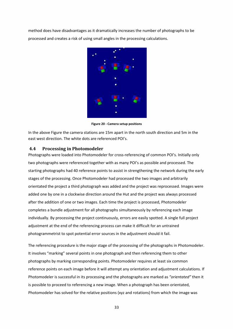
33
method does have disadvantages as it dramatically increases the number of photographs to be
processed and creates a risk of using small angles in the processing calculations.
Figure 20 - Camera setup positions
In the above Figure the camera stations are 15m apart in the north south direction and 5m in the
east west direction. The white dots are referenced POI’s.
4.4 Processing in Photomodeler
Photographs were loaded into Photomodeler for cross-referencing of common POI’s. Initially only
two photographs were referenced together with as many POI’s as possible and processed. The
starting photographs had 40 reference points to assist in strengthening the network during the early
stages of the processing. Once Photomodeler had processed the two images and arbitrarily
orientated the project a third photograph was added and the project was reprocessed. Images were
added one by one in a clockwise direction around the Hut and the project was always processed
after the addition of one or two images. Each time the project is processed, Photomodeler
completes a bundle adjustment for all photographs simultaneously by referencing each image
individually. By processing the project continuously, errors are easily spotted. A single full project
adjustment at the end of the referencing process can make it difficult for an untrained
photogrammetrist to spot potential error sources in the adjustment should it fail.
The referencing procedure is the major stage of the processing of the photographs in Photomodeler.
It involves “marking” several points in one photograph and then referencing them to other
photographs by marking corresponding points. Photomodeler requires at least six common
reference points on each image before it will attempt any orientation and adjustment calculations. If
Photomodeler is successful in its processing and the photographs are marked as “orientated” then it
is possible to proceed to referencing a new image. When a photograph has been orientated,
Photomodeler has solved for the relative positions (xyz and rotations) from which the image was
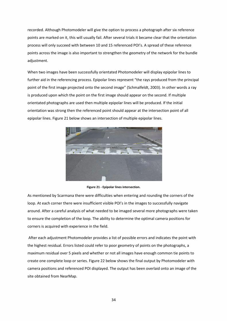
34
recorded. Although Photomodeler will give the option to process a photograph after six reference
points are marked on it, this will usually fail. After several trials it became clear that the orientation
process will only succeed with between 10 and 15 referenced POI’s. A spread of these reference
points across the image is also important to strengthen the geometry of the network for the bundle
adjustment.
When two images have been successfully orientated Photomodeler will display epipolar lines to
further aid in the referencing process. Epipolar lines represent “the rays produced from the principal
point of the first image projected onto the second image” (Schmalfeldt, 2003). In other words a ray
is produced upon which the point on the first image should appear on the second. If multiple
orientated photographs are used then multiple epipolar lines will be produced. If the initial
orientation was strong then the referenced point should appear at the intersection point of all
epipolar lines. Figure 21 below shows an intersection of multiple epipolar lines.
Figure 21 - Epipolar lines intersection.
As mentioned by Scarmana there were difficulties when entering and rounding the corners of the
loop. At each corner there were insufficient visible POI’s in the images to successfully navigate
around. After a careful analysis of what needed to be imaged several more photographs were taken
to ensure the completion of the loop. The ability to determine the optimal camera positions for
corners is acquired with experience in the field.
After each adjustment Photomodeler provides a list of possible errors and indicates the point with
the highest residual. Errors listed could refer to poor geometry of points on the photographs, a
maximum residual over 5 pixels and whether or not all images have enough common tie points to
create one complete loop or series. Figure 22 below shows the final output by Photomodeler with
camera positions and referenced POI displayed. The output has been overlaid onto an image of the
site obtained from NearMap.
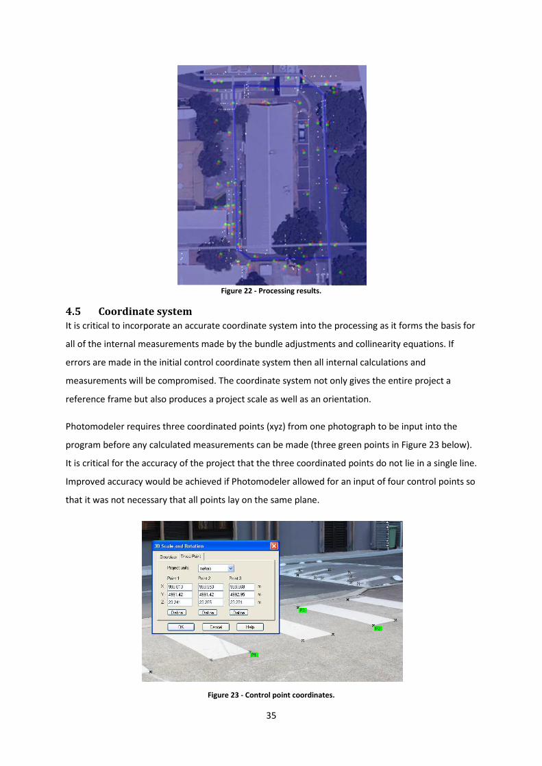
35
Figure 22 - Processing results.
4.5 Coordinate system
It is critical to incorporate an accurate coordinate system into the processing as it forms the basis for
all of the internal measurements made by the bundle adjustments and collinearity equations. If
errors are made in the initial control coordinate system then all internal calculations and
measurements will be compromised. The coordinate system not only gives the entire project a
reference frame but also produces a project scale as well as an orientation.
Photomodeler requires three coordinated points (xyz) from one photograph to be input into the
program before any calculated measurements can be made (three green points in Figure 23 below).
It is critical for the accuracy of the project that the three coordinated points do not lie in a single line.
Improved accuracy would be achieved if Photomodeler allowed for an input of four control points so
that it was not necessary that all points lay on the same plane.
Figure 23 - Control point coordinates.
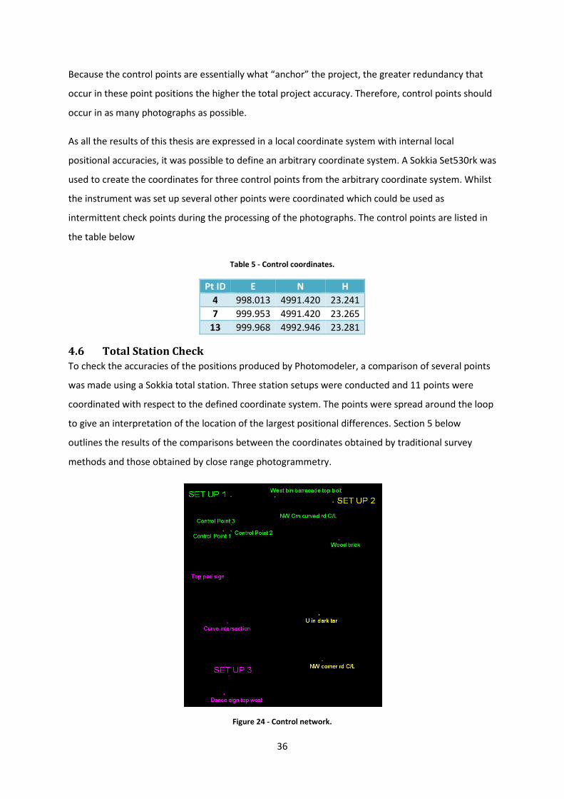
36
Because the control points are essentially what “anchor” the project, the greater redundancy that
occur in these point positions the higher the total project accuracy. Therefore, control points should
occur in as many photographs as possible.
As all the results of this thesis are expressed in a local coordinate system with internal local
positional accuracies, it was possible to define an arbitrary coordinate system. A Sokkia Set530rk was
used to create the coordinates for three control points from the arbitrary coordinate system. Whilst
the instrument was set up several other points were coordinated which could be used as
intermittent check points during the processing of the photographs. The control points are listed in
the table below
Table 5 - Control coordinates.
Pt ID E N H
4 998.013 4991.420 23.241
7 999.953 4991.420 23.265
13 999.968 4992.946 23.281
4.6 Total Station Check
To check the accuracies of the positions produced by Photomodeler, a comparison of several points
was made using a Sokkia total station. Three station setups were conducted and 11 points were
coordinated with respect to the defined coordinate system. The points were spread around the loop
to give an interpretation of the location of the largest positional differences. Section 5 below
outlines the results of the comparisons between the coordinates obtained by traditional survey
methods and those obtained by close range photogrammetry.
Figure 24 - Control network.
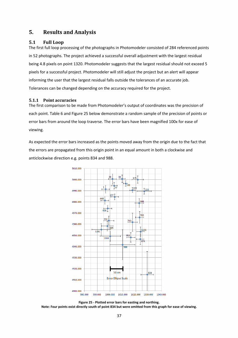
37
5. Results and Analysis
5.1 Full Loop The first full loop processing of the photographs in Photomodeler consisted of 284 referenced points
in 52 photographs. The project achieved a successful overall adjustment with the largest residual
being 4.8 pixels on point 1320. Photomodeler suggests that the largest residual should not exceed 5
pixels for a successful project. Photomodeler will still adjust the project but an alert will appear
informing the user that the largest residual falls outside the tolerances of an accurate job.
Tolerances can be changed depending on the accuracy required for the project.
5.1.1 Point accuracies
The first comparison to be made from Photomodeler’s output of coordinates was the precision of
each point. Table 6 and Figure 25 below demonstrate a random sample of the precision of points or
error bars from around the loop traverse. The error bars have been magnified 100x for ease of
viewing.
As expected the error bars increased as the points moved away from the origin due to the fact that
the errors are propagated from this origin point in an equal amount in both a clockwise and
anticlockwise direction e.g. points 834 and 988.
Figure 25 - Plotted error bars for easting and northing.
Note: Four points exist directly south of point 834 but were omitted from this graph for ease of viewing.
38
Table 6 - Positional precisions.
At the beginning of the loop the error bars are in the magnitude of 2-3 cm in the x direction and 3-4
cm in the y direction. It would initially be assumed that the error bars would be similar in both
directions as no significant gross errors have yet been introduced into the project and the errors
would consist only of random errors.
The precision in the x direction ranges from 1.6 cm to 22 cm and 2 cm to 58 cm in the y direction.
Both maximum values occurred at point 838 which was 120 m from the starting point. Points 828,
836, 838 and 856 all have significantly worse precisions in all directions when compared to all other
points in the loop. In particular, the y and z precision components of these points are in excess of
two times larger than all other points. This sudden jump in precision is attributed to the fact that
they were taken from a distance of over 50m and appear in only two photographs. Clearly marking a
point at such a distance is difficult as the image becomes blurred and pixelated as the photograph is
enlarged.
Point ID X Precision
(cm)
Y Precision
(cm)
Z Precision
(cm)
1 2.749 3.533 0.014
20 3.058 4.532 0.016
30 2.419 3.441 0.011
77 2.301 2.904 0.010
166 1.728 2.573 0.004
175 4.288 3.230 0.010
233 5.429 2.541 0.012
277 2.286 2.176 0.006
377 2.631 2.592 0.006
436 2.735 2.784 0.006
448 2.730 3.332 0.009
551 3.283 3.896 0.011
644 3.269 3.654 0.006
743 3.525 8.105 0.011
783 2.965 5.052 0.006
834 4.917 20.770 0.026
870 3.083 4.802 0.009
913 2.948 4.186 0.006
988 9.418 13.280 0.010
1060 7.490 4.335 0.011
1155 3.128 4.182 0.007
1281 7.068 5.245 0.016
1309 3.834 4.173 0.011
39
Although Scarmana does not record the precisions he achieved in his project based on final results, it
would be assumed that they would be of a similar magnitude.
5.1.2 AutoCAD Comparisons
The best comparison that can be made is between coordinates that are produced by Photomodeler
and the control points coordinated using the Sokkia total station. Table 7 below is an output of
coordinates of 13 randomly distributed points around the loop and the differences in their
coordinates.
Table 7 - Coordinate Comparison.
From Table 7 above it can be seen that the discrepancy in coordinates between Photomodeler’s
adjustment and the control points get larger as the points travel away from the defined points (4, 7
and 13). This is as expected as, with any loop traverse, the errors are increased with respect to the
distance from the control points held fixed. At point 834, which is furthest from the three control
points held fixed, the errors are the largest in all three directions. The maximum average error
obtained from this project was 0.651 m in the horizontal positioning of the point. As Scarmana
achieved an average error of 1m for every 150 m travelled in the horizontal positional direction it
was assumed the error would be of a similar magnitude. The height component for all points is
significantly smaller than the x and y components due to the points all lying on the ground. Any
points that are raised significantly have a considerably larger error in height.
As the samples analysed her are a random selection of the data points, it is expected that the overall
project accuracy is in this range. The positional accuracies also correlate with the x and y precisions
CAD Coordinates Photo coordinates Difference
Order
From
Start
Pt ID E N H E N H E N H
1 4 998.013 4991.420 23.241 998.013 4991.420 23.241 0 0 0
2 7 999.953 4991.420 23.265 999.953 4991.420 23.265 0 0 0
3 13 999.968 4992.946 23.281 999.966 4992.952 23.281 -0.0019 0.0063 0.0000
4 1458 1004.071 4995.490 23.365 1004.078 4995.535 23.356 0.0075 0.0445 -0.0091
5 22 1010.893 4999.946 24.747 1010.816 4999.979 24.712 -0.0771 0.0329 -0.0346
6 230 1017.339 4996.493 23.525 1017.195 4996.621 23.501 -0.1439 0.1278 -0.0244
7 233 1026.778 4989.269 23.899 1026.488 4989.662 23.865 -0.2901 0.3931 -0.0336
8 722 1021.898 4970.571 23.364 1022.104 4971.218 23.413 0.2069 0.6469 0.0493
9 1154 1022.663 4959.123 23.237 1023.116 4959.563 23.328 0.4526 0.4401 0.0909
10 834 1028.364 4915.372 25.512 1027.844 4915.932 25.817 0.4808 -0.4404 0.3047
11 1259 998.268 4950.752 25.024 998.324 4950.435 25.069 0.0552 -0.3170 0.0454
12 439 999.015 4968.549 23.026 998.986 4968.333 23.031 -0.0289 -0.2157 0.0052
13 449 995.900 4981.409 25.737 995.895 4981.286 25.722 -0.0043 -0.1230 -0.0149
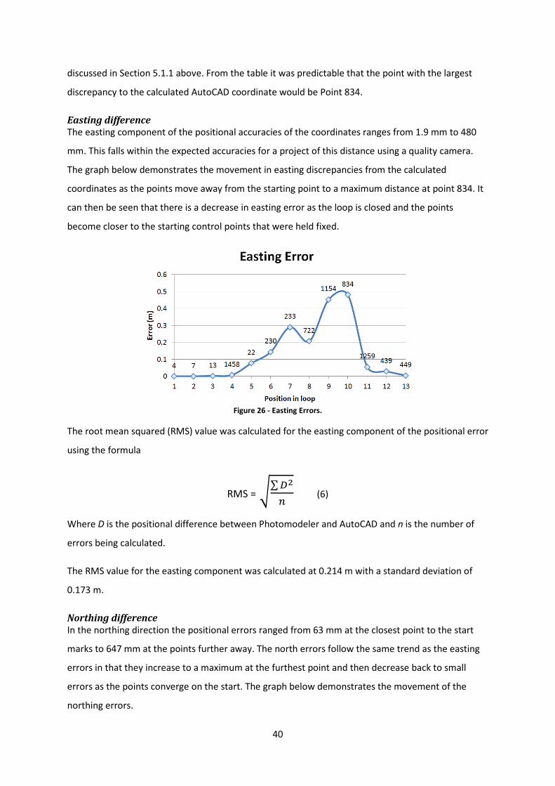
40
discussed in Section 5.1.1 above. From the table it was predictable that the point with the largest
discrepancy to the calculated AutoCAD coordinate would be Point 834.
Easting difference
The easting component of the positional accuracies of the coordinates ranges from 1.9 mm to 480
mm. This falls within the expected accuracies for a project of this distance using a quality camera.
The graph below demonstrates the movement in easting discrepancies from the calculated
coordinates as the points move away from the starting point to a maximum distance at point 834. It
can then be seen that there is a decrease in easting error as the loop is closed and the points
become closer to the starting control points that were held fixed.
Figure 26 - Easting Errors.
The root mean squared (RMS) value was calculated for the easting component of the positional error
using the formula
RMS = ∑ ��� (6)
Where D is the positional difference between Photomodeler and AutoCAD and n is the number of
errors being calculated.
The RMS value for the easting component was calculated at 0.214 m with a standard deviation of
0.173 m.
Northing difference
In the northing direction the positional errors ranged from 63 mm at the closest point to the start
marks to 647 mm at the points further away. The north errors follow the same trend as the easting
errors in that they increase to a maximum at the furthest point and then decrease back to small
errors as the points converge on the start. The graph below demonstrates the movement of the
northing errors.
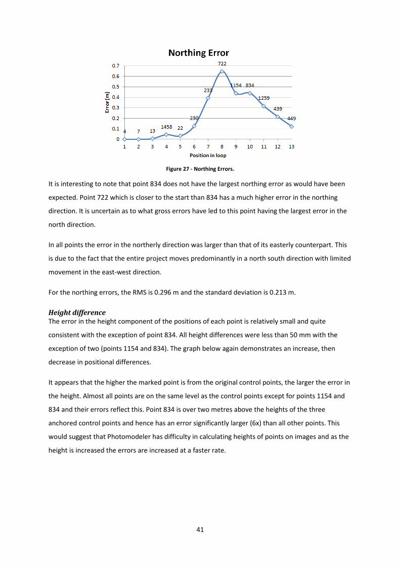
41
Figure 27 - Northing Errors.
It is interesting to note that point 834 does not have the largest northing error as would have been
expected. Point 722 which is closer to the start than 834 has a much higher error in the northing
direction. It is uncertain as to what gross errors have led to this point having the largest error in the
north direction.
In all points the error in the northerly direction was larger than that of its easterly counterpart. This
is due to the fact that the entire project moves predominantly in a north south direction with limited
movement in the east-west direction.
For the northing errors, the RMS is 0.296 m and the standard deviation is 0.213 m.
Height difference
The error in the height component of the positions of each point is relatively small and quite
consistent with the exception of point 834. All height differences were less than 50 mm with the
exception of two (points 1154 and 834). The graph below again demonstrates an increase, then
decrease in positional differences.
It appears that the higher the marked point is from the original control points, the larger the error in
the height. Almost all points are on the same level as the control points except for points 1154 and
834 and their errors reflect this. Point 834 is over two metres above the heights of the three
anchored control points and hence has an error significantly larger (6x) than all other points. This
would suggest that Photomodeler has difficulty in calculating heights of points on images and as the
height is increased the errors are increased at a faster rate.
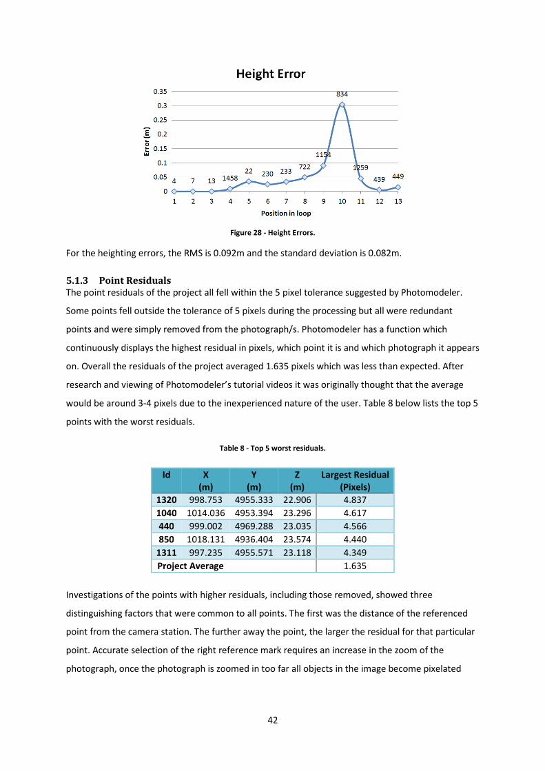
42
Figure 28 - Height Errors.
For the heighting errors, the RMS is 0.092m and the standard deviation is 0.082m.
5.1.3 Point Residuals
The point residuals of the project all fell within the 5 pixel tolerance suggested by Photomodeler.
Some points fell outside the tolerance of 5 pixels during the processing but all were redundant
points and were simply removed from the photograph/s. Photomodeler has a function which
continuously displays the highest residual in pixels, which point it is and which photograph it appears
on. Overall the residuals of the project averaged 1.635 pixels which was less than expected. After
research and viewing of Photomodeler’s tutorial videos it was originally thought that the average
would be around 3-4 pixels due to the inexperienced nature of the user. Table 8 below lists the top 5
points with the worst residuals.
Table 8 - Top 5 worst residuals.
Investigations of the points with higher residuals, including those removed, showed three
distinguishing factors that were common to all points. The first was the distance of the referenced
point from the camera station. The further away the point, the larger the residual for that particular
point. Accurate selection of the right reference mark requires an increase in the zoom of the
photograph, once the photograph is zoomed in too far all objects in the image become pixelated
Id X
(m)
Y
(m)
Z
(m)
Largest Residual
(Pixels)
1320 998.753 4955.333 22.906 4.837
1040 1014.036 4953.394 23.296 4.617
440 999.002 4969.288 23.035 4.566
850 1018.131 4936.404 23.574 4.440
1311 997.235 4955.571 23.118 4.349
Project Average 1.635
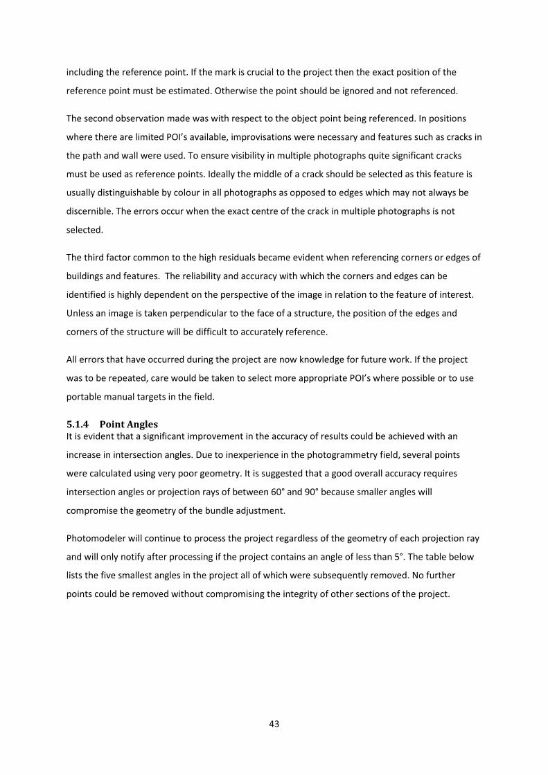
43
including the reference point. If the mark is crucial to the project then the exact position of the
reference point must be estimated. Otherwise the point should be ignored and not referenced.
The second observation made was with respect to the object point being referenced. In positions
where there are limited POI’s available, improvisations were necessary and features such as cracks in
the path and wall were used. To ensure visibility in multiple photographs quite significant cracks
must be used as reference points. Ideally the middle of a crack should be selected as this feature is
usually distinguishable by colour in all photographs as opposed to edges which may not always be
discernible. The errors occur when the exact centre of the crack in multiple photographs is not
selected.
The third factor common to the high residuals became evident when referencing corners or edges of
buildings and features. The reliability and accuracy with which the corners and edges can be
identified is highly dependent on the perspective of the image in relation to the feature of interest.
Unless an image is taken perpendicular to the face of a structure, the position of the edges and
corners of the structure will be difficult to accurately reference.
All errors that have occurred during the project are now knowledge for future work. If the project
was to be repeated, care would be taken to select more appropriate POI’s where possible or to use
portable manual targets in the field.
5.1.4 Point Angles
It is evident that a significant improvement in the accuracy of results could be achieved with an
increase in intersection angles. Due to inexperience in the photogrammetry field, several points
were calculated using very poor geometry. It is suggested that a good overall accuracy requires
intersection angles or projection rays of between 60° and 90° because smaller angles will
compromise the geometry of the bundle adjustment.
Photomodeler will continue to process the project regardless of the geometry of each projection ray
and will only notify after processing if the project contains an angle of less than 5°. The table below
lists the five smallest angles in the project all of which were subsequently removed. No further
points could be removed without compromising the integrity of other sections of the project.
44
Table 9 - Top 5 worst angles.
The final project had angles ranging from 5° to 90° with an average of 46° and a median of 48°. This
is well below what is recommended as the standard in the photogrammetry field.
However, there were sections of the loop that required small angles due to the limited space. In
areas where the field of view was limited it was necessary to compromise between using small
angles and capturing enough POI’s to reference to other photographs. The area in the south west
corner of this traverse in particular was difficult due to the narrow path between two opposing
buildings.
Based on the results of this project, it is evident that, with further experience in the field of
photogrammetry, it would be possible to set the camera stations closer to optimal positions.
Network geometry is crucial to the project accuracy and without doubt the accuracy of this project
could be increased with improvement in the ray intersection angles.
5.2 Incomplete Loop For comparison purposes, the project was processed again with several photographs set to “Do not
use”. To gain an accurate reading of the types of errors that occur when the loop is incomplete there
should be no connection between the photographs at the start and end of the loop. Because almost
all of the photographs on the western side of the loop use points from photographs 2 and 3 to
orientate themselves, fifteen photographs (19, 21-29, 31-32, 68 and 71-72) were taken from the
loop before it was reprocessed. Figure 29 below illustrates the incomplete loop.
Figure 29 - Incomplete loop.
Id X (m) Y (m) Z (m) Angle (Deg)
1236 986.7559 4951.1904 24.1825 3.1971
1240 999.4663 4949.7927 24.5948 3.3315
1242 999.4929 4949.7953 24.6412 3.3500
1238 986.6303 4950.8839 25.2835 3.4244
1244 986.6797 4952.2778 23.7052 3.6611
Project Average 46.6224
45
5.2.1 Point accuracies
The point accuracies for a random distribution of points around the incomplete loop can be seen
below in Figure 30. As expected, the errors are larger across both the x and y directions with the x
precision being an average of 3 cm bigger and the y precision 1 cm bigger than when the loop was
closed.
Figure 30 - Plotted easting and northing error bars.
There appears to be no obvious pattern to the amount variation in precision as the traverse
progresses around the loop. Point 838 again has the lowest precisions in the y and z directions with
precision values of 52 cm and 5 cm respectively. The worst precision in the x direction is point 1281
which occurs at the end of the traverse line with a value of 20 cm.
It was expected that the precision values would increase with the incomplete loop because, without
a join, the entire project is free to move or rotate independent of other marks. In a completed loop
the project will move as whole.
46
Table 10 - Precision Comparisons.
The precisions of the incomplete loop are approximately 1.9 and 1.2 times larger in the x and y
directions respectively. This implies that when the loop is not complete some points will have lower
accuracy precision than when the loop is complete.
There were, however, several points, particularly in the y direction, that showed a higher precision
when the loop was incomplete. This suggests that the precision levels are highly dependent on the
expertise of the operator, rather than on the computer software.
5.2.2 AutoCAD Comparisons
In a general surveying traverse if the loop is not closed, errors will propagate down the length of the
traverse with the maximum error occurring at the end of the traverse length. Unless the loop is
closed it is impossible to spread any gross errors throughout the entire project so they are all
accumulated. As shown in Table 11 below this is what occurred in this project.
The discrepancies in the positional values accumulate as the points move around the traverse to an
error of almost 1 m in the x direction, 1.8 m in the y and 0.5 m in height. This shift of the final point
has compromised the accuracy of the project to a point where it no longer meets the accuracy
guidelines set by Scarmana in his project.
Point
ID
X Precision (cm) Y Precision (cm)
Full
Loop
Incomplete
Loop
Difference Full
Loop
Incomplete
Loop
Difference
cm % cm %
1 2.749 10.095 7.346 267.22 3.533 5.624 2.091 59.18
20 3.058 6.843 3.785 123.77 4.532 7.559 3.027 66.79
30 2.419 3.062 0.643 26.58 3.441 5.265 1.824 53.01
77 2.301 6.083 3.782 164.36 2.904 4.036 1.132 38.98
166 1.728 1.914 0.186 10.76 2.573 3.231 0.658 25.57
175 4.288 4.784 0.496 11.57 3.230 3.967 0.737 22.82
233 5.429 6.331 0.902 16.61 2.541 3.014 0.473 18.61
277 2.286 1.842 - 0.444 19.42 2.176 2.063 - 0.113 5.19
644 2.631 3.097 0.466 17.71 3.654 5.367 1.713 46.88
743 2.735 3.261 0.526 19.23 8.105 7.254 - 0.851 10.50
783 2.730 2.658 - 0.072 2.64 5.052 6.806 1.754 34.72
834 3.283 9.014 5.731 174.57 20.770 18.825 - 1.945 9.36
870 3.269 4.144 0.875 26.77 4.802 4.593 - 0.209 4.35
913 3.525 3.126 - 0.399 11.32 4.186 3.988 - 0.198 4.73
988 2.965 9.583 6.618 223.20 13.280 13.897 0.617 4.65
1060 4.917 7.607 2.69 54.71 4.335 4.200 - 0.135 3.11
1155 3.083 3.711 0.628 20.37 4.182 4.658 0.476 11.38
1281 2.948 20.310 17.362 588.94 5.245 6.139 0.894 17.04
1309 9.418 8.907 - 0.511 5.43 4.173 5.719 1.546 37.05
Average 2.8138 93.96 1.0733 24.94
47
Table 11 - AutoCAD Comparison.
Although the northing component of several positions was closer than expected when the loop was
incomplete, this was counteracted by significantly poorer easting and height components
The graph below shows the errors in all directions as the traverse moves around the loop. It appears
that errors are exponential for all components, where errors are reasonably small at the start of the
traverse and increase to 1.8 m for the northing direction near the end of the traverse.
Figure 31 - ENH errors for incomplete loop.
From the data it can be concluded that, without the closure of a loop, the positional data output
from Photomodeler is of almost no use. To be over 2 m from the intended destination after
Full Loop Coordinates Incomplete Loop coordinates Difference %
Pt ID E N H E N H E N H
4 0 0 0 0 0 0 0 0 0
7 0 0 0 0 0 0 0 0 0
13 -0.0019 0.0063 0.0000 -0.0096 -0.0007 -0.0001 505.26 11.11 0
1458 0.0075 0.0445 -0.0091 -0.0171 0.0273 -0.0124 228.00 61.35 136.26
22 -0.0771 0.0329 -0.0346 -0.0944 0.0357 -0.0491 122.44 108.51 141.91
230 -0.1439 0.1278 -0.0244 -0.1114 0.1425 -0.0314 77.41 111.50 128.69
233 -0.2901 0.3931 -0.0336 -0.1496 0.3886 -0.0135 51.57 98.86 40.18
722 0.2069 0.6469 0.0493 0.4932 0.5421 0.1399 238.38 83.80 283.77
1154 0.4526 0.4401 0.0909 0.7936 0.6598 0.2290 175.34 149.92 251.93
834 0.4808 -0.4404 0.3047 0.9536 1.834 0.547 198.34 416.44 179.52
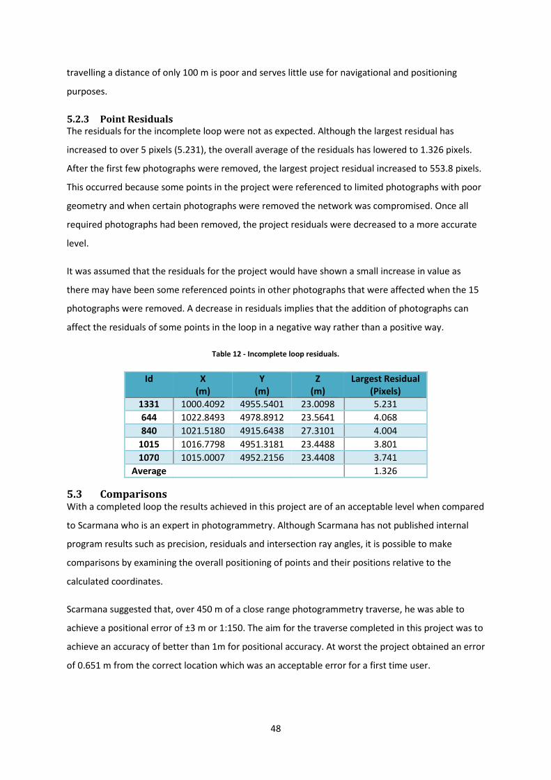
48
travelling a distance of only 100 m is poor and serves little use for navigational and positioning
purposes.
5.2.3 Point Residuals
The residuals for the incomplete loop were not as expected. Although the largest residual has
increased to over 5 pixels (5.231), the overall average of the residuals has lowered to 1.326 pixels.
After the first few photographs were removed, the largest project residual increased to 553.8 pixels.
This occurred because some points in the project were referenced to limited photographs with poor
geometry and when certain photographs were removed the network was compromised. Once all
required photographs had been removed, the project residuals were decreased to a more accurate
level.
It was assumed that the residuals for the project would have shown a small increase in value as
there may have been some referenced points in other photographs that were affected when the 15
photographs were removed. A decrease in residuals implies that the addition of photographs can
affect the residuals of some points in the loop in a negative way rather than a positive way.
Table 12 - Incomplete loop residuals.
5.3 Comparisons With a completed loop the results achieved in this project are of an acceptable level when compared
to Scarmana who is an expert in photogrammetry. Although Scarmana has not published internal
program results such as precision, residuals and intersection ray angles, it is possible to make
comparisons by examining the overall positioning of points and their positions relative to the
calculated coordinates.
Scarmana suggested that, over 450 m of a close range photogrammetry traverse, he was able to
achieve a positional error of ±3 m or 1:150. The aim for the traverse completed in this project was to
achieve an accuracy of better than 1m for positional accuracy. At worst the project obtained an error
of 0.651 m from the correct location which was an acceptable error for a first time user.
Id X
(m)
Y
(m)
Z
(m)
Largest Residual
(Pixels)
1331 1000.4092 4955.5401 23.0098 5.231
644 1022.8493 4978.8912 23.5641 4.068
840 1021.5180 4915.6438 27.3101 4.004
1015 1016.7798 4951.3181 23.4488 3.801
1070 1015.0007 4952.2156 23.4408 3.741
Average 1.326

49
Although the accuracies and quality of this project are based on the results obtained by Scarmana
there were some differences in the project that would have influenced the results. Scarmana
obtained his results using an off the shelf camera with a quality of 5 megapixels which by today’s
standard is low. The Canon EOS 450D 12 megapixel camera used for this project, has a far higher
image sensor. As the quality of the camera is one of the major influencing factors on the quality of
the results it would be expected that the results obtained in this thesis project would be far more
accurate than those obtained using an inferior camera.
However, in opposition to the quality of the camera is the capability of the user. Scarmana is an
expert in the photogrammetric field and has had many years of experience in both field applications
and teaching at the University of Southern Queensland. It would be expected that Scarmana would
produce the best possible results with the instrumentation used. This thesis project was completed
by a user completely inexperienced in photogrammetric techniques. A lack of instinctive knowledge
of factors such as where to best place camera stations, best types of POI’s to photograph and how
the geometry will affect the overall positional accuracy of the job contributed to the quality of the
final results.
A higher quality camera was used for this project in an effort to compensate for Scarmana’s higher
level of expertise. After analysing the final results it was determined that the quality of the camera
probably contributes more to the positional accuracies than the experience of the operator. The
ability to capture high quality images and points of interest is important as it allows for accurate
referencing of photographs in Photomodeler.
50
6. Conclusions The aim of this thesis was to determine whether or not a non-photogrammetric expert could
reproduce the results of the project presented by Gabriel Scarmana at the 2010 FIG conference in
Sydney to a similar accuracy. Scarmana outlined a photogrammetric “reconstruction technique for
trajectory reconstruction without GPS navigation tools” (Scarmana, 2010). As outlined above in
Section 5 the results obtained by this thesis are consistent with the results obtained by Scarmana.
The overall positional accuracy of the coordinates produced by Photomodeler when the loop is
complete is within 0.651 m from the results obtained using a conventional surveying technique.
Scarmana had suggested that an error of 1m for every 150 m travelled should be expected. The total
length of the traverse in this project was 140 m, thus positional accuracy was estimated to be just
less than 1m. The 0.651 m error is better than this estimate. An incomplete loop produced
positional inaccuracies up to 2 m in magnitude, suggesting that the traverse must be a complete
loop if it is to be of use for surveyors.
The quality of the camera is the most significant factor in the quality of positional accuracy of this
method. This project used a camera with 12 megapixels which is significantly higher to the 5
megapixel camera used by Scarmana. The indifference in camera quality makes it difficult to
compare accuracies but it can be concluded that the use of a higher quality camera probably
accounted for the lack of experience in photogrammetry. The results obtained in this thesis were of
a higher accuracy to Scarmana’s which can be attributed to the quality of camera used.
During the completion of this thesis several distinguishing factors were identified that affected the
accuracy of the overall project. The first factor noted was that a successfully orientated photograph
requires at least ten referenced points in the image. Photomodeler will inform the user that the
photograph may orientate after only six points have been referenced but the program will usually
fail in its orientation attempt. To ensure accuracy is maintained it is considered good practice to wait
until at least ten or more points are referenced on the photograph.
Further to this, it is important that the points used as reference marks are well spread across the
photograph. Spreading points across the photograph, including points in both the foreground and
background, allows for a strong geometry in the collinearity equations that are produced. A stronger
geometry in the network calculations produces a more reliable and accurate result for the project. It
is important not to include any points that you are unsure of, as less reference points in an image is
preferable to poorly referenced points.
51
The positional accuracy of the selected POI also deteriorates with the distance from the control
points. These positional errors were affected not only by the distance covered but also by the
number of observation or camera stations, the precision of the referenced points and the measuring
geometry.
Photomodeler is a well suited program for the close-range photogrammetry application that was
applied in this thesis. It is possible to produce an accurate result without a high level of expertise in
this software. Some knowledge of photogrammetry would be useful when recording images to
ensure that sufficient image overlap and angular separation between camera stations was
maintained.
When calibrating an instrument in Photomodeler it is important to note that the calibration program
will pick up more than the calibration grid in the images. Care must be taken when selecting the area
for the calibration as a dark speckled background will introduce errors. The calibration will also not
work if the calibration grid is printed on glossy paper. Photomodeler does not recognise the points
when processing the images as the reflection of the lights and flash will cause points to become sub-
pixel. To overcome this issue the calibration grid must be printed on matt paper.
The 12x12 calibration grid gave errors 100x greater than the results produced by the 10x10 grid. The
cause of this is still unknown so it is suggested that for an accurate calibration it is good practice to
use the 10x10 grid. It is crucial to plan the station setups for the calibration process as there is a
requirement for an accurate calibration that there at least 80% of the image plane of the camera
covered.
From the experiences gained during this thesis there are several recommendations that would be
made for anyone undertaking similar future work. One recommendation for any future work would
be the addition of portable targets for areas containing limited POI’s. In this project the geometry
was compromised to ensure there were sufficient POI’s in the image, however adding portable POI’s
to the field of view would allow ideal geometry to be maintained. Having portable targets would
allow you to position the camera in a place where the geometry would be strongest and then targets
could be placed so they were in the field of view.
Another suggestion would be to investigate the use of coded targets throughout the project to
achieve a quicker and more accurate result. The most time consuming and therefore inefficient
aspect of the project involved the referencing of POI’s on multiple photographs. It took around six to
seven hours to process the 54 photographs manually with high precision. If coded targets are used,
Photomodeler’s recognition function will automatically reference a target in all images in which it

52
appears. This would significantly reduce image processing time and make the method more
attractive for everyday use.
When a coordinate system is introduced into Photomodeler it defined by assigning coordinates to
three control points only. Fixing three control points is the minimum required to fully define a three
dimensional coordinate system. If Photomodeler had allowed for a fourth control point, redundancy
would have been created. It would have also introduced a point that was on a different plane to the
other three. It would be a simple task for EOS Systems to introduce a forth control point into the
coordinate system definition and it is believed that accuracy would be improved.
Further studies with additional camera stations and improved camera angles should be conducted to
determine the effects that they may have on improving accuracy. There is no doubt that both factors
influence the accuracies of the project but it is uncertain how much each factor directly affects the
projects accuracies.
Using close range photogrammetry as a means of positioning and navigation is a relatively new
method and has potential for future development and investigation. Investigation into the quality
that could be achieved using a Smartphone is suggested. As Smartphone’s become increasingly
popular, an application which incorporates Scarmana’s ideas is a possible future development. If an
acceptable level of navigational accuracies could be achieved from an 8 megapixel mobile phone, a
range of photogrammetry applications could be made readily available for popular use.
These results should be compared to those obtained using alternative software programs such as
Australis or iWitness. This would provide some insight into whether accuracy is limited by camera or
by software. All software programs have advantages and disadvantages which can make the
processing easier or harder.
Overall, this project was successful in demonstrating that an inexperienced user in the
photogrammetric field can reproduce the results obtained by Scarmana to an acceptable level. With
additional experience it would be possible to improve on Scarmana’s results given the quality of
instruments used throughout the duration of this project.
53
6 References 1. Atkinson K.B. (1996). Close Range Photogrammetry and Machine Vision. Whittles Publishing,
Scotland.
2. Clemente L., Davison A., Reid I. D., Neira J. and Tardós J. (2008). “Mapping Large Loops with
a Single Hand-Held Camera”. Robotics: Science and Systems III, June 27-30, 2007, Georgia
Institute of Technology, Atlanta, Georgia, USA 2008.
3. Cooper M., Robson S. (1996) Chapter 2: Theory of Close Range Photogrammetry, Atkinson,
K.B. editor, Close Range Photogrammetry and Machine Vision, Whittles Publishing, Scotland,
pp. 9-50
4. Dowman I. (1996) Chapter 3: Fundamentals of digital photography, Atkinson, K.B. editor,
Close Range Photogrammetry and Machine Vision, Whittles Publishing, Scotland, pp. 1-6
5. EOS Systems Inc (2011) Photomodeler Pro online Tutorials. Available from
<http://www.photomodeler.com/tutorial-vids/online-tutorials.htm> (Accessed 11
April,2011)
6. Faig, W. (1986), Aerial Triangulation and Digital Mapping, Monograph 10, School Of
Surveying And Spatial Information Systems UNSW Scarmana, G. (2010), Mapping in a City
Environment using a Single Hand-Held Digital Camera. FIG Congress 2010, Facing the
Challenges – Building the Capacity, Sydney, Australia, 11-16 April 2010
7. Fryer, J.G. (1985) Non-Metric Photogrammetry and Surveyors. The Australian Surveyor
Vol.32 No.5 March 1985, pg 330-341
8. Fryer, J.G. (1996a) Chapter 1: Introduction, Atkinson, K.B. editor, Close Range
Photogrammetry and Machine Vision, Whittles Publishing, Scotland, pp. 1-6
9. Fryer, J.G. (1996b) Chapter 6: Camera Calibration, Atkinson, K.B. editor, Close Range
Photogrammetry and Machine Vision, Whittles Publishing, Scotland, pp. 156-179
10. Geodetic surveyors Inc. (2006). The Basics of Photogrammetry. Available form:
<http://www.geodetic.com/whatis.htm> (accessed 26 March)
11. Luhman T., Robson S., Kyle S. and Harley I. (2006) Close Range Photogrammetry: Principals,
Methods and Applications, Whittles Publishing, Scotland, pp 1-12
12. Marshall, AR. (1989), Network Design and Optimisation in Close Range Photogrammetry,
Unisurv S-36, School of Surveying and Spatial Information Systems UNSW.
13. Oxford Dictionary. (2011) Oxford University Press. Available form: < http://www.oed.com/>
(accessed 15 October)
14. Schmalfeldt, L. (2003) Application of Photomodeler Pro 5 Software. Thesis, University of
New South Wales.

54
15. Trinder, J. (2011) Chapter 7: Close Range Photogrammetry. GMAT9300 Aerial and Satellite
Imaging Systems Lecture slides, University of New South Wales.
55
7. Bibliography 1. Fedak M. (2006)3D Measurement Accuracy of a Consumer-Grade Digital Camera and Retro-
Reflective Survey Targets. Available from
<http://www.photomodeler.com/applications/documents/fedak1.pdf> (Accessed 24 April,
2011)
2. Fraser C. (1996). Chapter 9: Network Design, Atkinson, K.B. editor, Close Range
Photogrammetry and Machine Vision, Whittles Publishing, Scotland, pp. 256-279
3. Gruen A. (1996). Chapter 4: Development of Digital methodology and systems, Atkinson, K.B.
editor, Close Range Photogrammetry and Machine Vision, Whittles Publishing, Scotland, pp.
78-99
4. Hotine, M. (1929). Calibration of Surveying Cameras. Royal Engineers, London pp 1-29
5. Maynard L., Dunn M Jr. (2003) Recent Developments in Close Range Photogrammetry (CRP)
for Mining and Reclamation. Office of Surface Mining and Reclamation Pittsburgh, PA.
Available from
<http://www.photomodeler.com/applications/documents/Dunn_Billings_PMS_Geology.pdf>
(Accessed 24 April, 2011)
6. Pappa R.S, Giersch L.R, Quagliaroli J.M. (2001). Photogrammetry of a 5m Inflatable Space
Antenna With Consumer Digital Cameras, Experimental Techniques (internet vol.25 (4) pp.
21-29) Available from <http://www.photomodeler.com/applications/documents/NASA.pdf>
(Accessed 24 April, 2011)
7. Sanz-Ablanedo E, Rodríguez-Pérez J.R, Arias-Sánchez P and Armesto J. (2009). Metric
Potential of a 3D Measurement System Based on Digital Compact Cameras, SENSORS
(internet vol 9 (6) pp. 4178-4194) Available from
<http://www.photomodeler.com/applications/documents/MetricPotentialMultipleConsume
rCameras.pdf> (Accessed 24 April, 2011)
8. Walford A. (2006). One Part in 300,000: Precision and Accuracy Discussion. Eos Systems Inc.
Available from <http://www.photomodeler.com/applications/documents/Precision.pdf>
(Accessed 24 April, 2011)
9. Yaker M. (2001). Using Close Range Photogrammetry to Measure the Position of Inaccessible
Geological Features, Experimental Techniques (internet vol.35 (1) pp. 54-59) Available from
<http://www.photomodeler.com/applications/documents/CRPforInaccessibleGeologicFeatu
res.pdf> (Accessed 24 April, 2011)
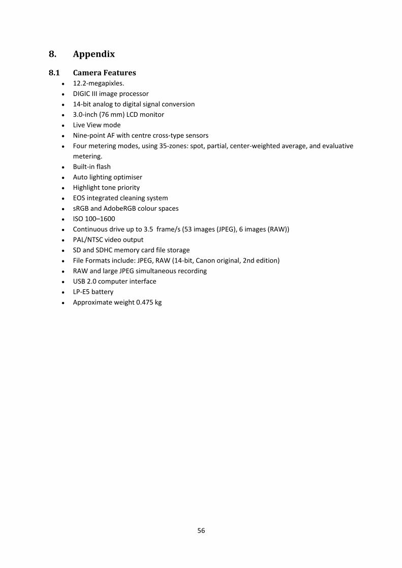
56
8. Appendix
8.1 Camera Features
• 12.2-megapixles.
• DIGIC III image processor
• 14-bit analog to digital signal conversion
• 3.0-inch (76 mm) LCD monitor
• Live View mode
• Nine-point AF with centre cross-type sensors
• Four metering modes, using 35-zones: spot, partial, center-weighted average, and evaluative
metering.
• Built-in flash
• Auto lighting optimiser
• Highlight tone priority
• EOS integrated cleaning system
• sRGB and AdobeRGB colour spaces
• ISO 100–1600
• Continuous drive up to 3.5 frame/s (53 images (JPEG), 6 images (RAW))
• PAL/NTSC video output
• SD and SDHC memory card file storage
• File Formats include: JPEG, RAW (14-bit, Canon original, 2nd edition)
• RAW and large JPEG simultaneous recording
• USB 2.0 computer interface
• LP-E5 battery
• Approximate weight 0.475 kg
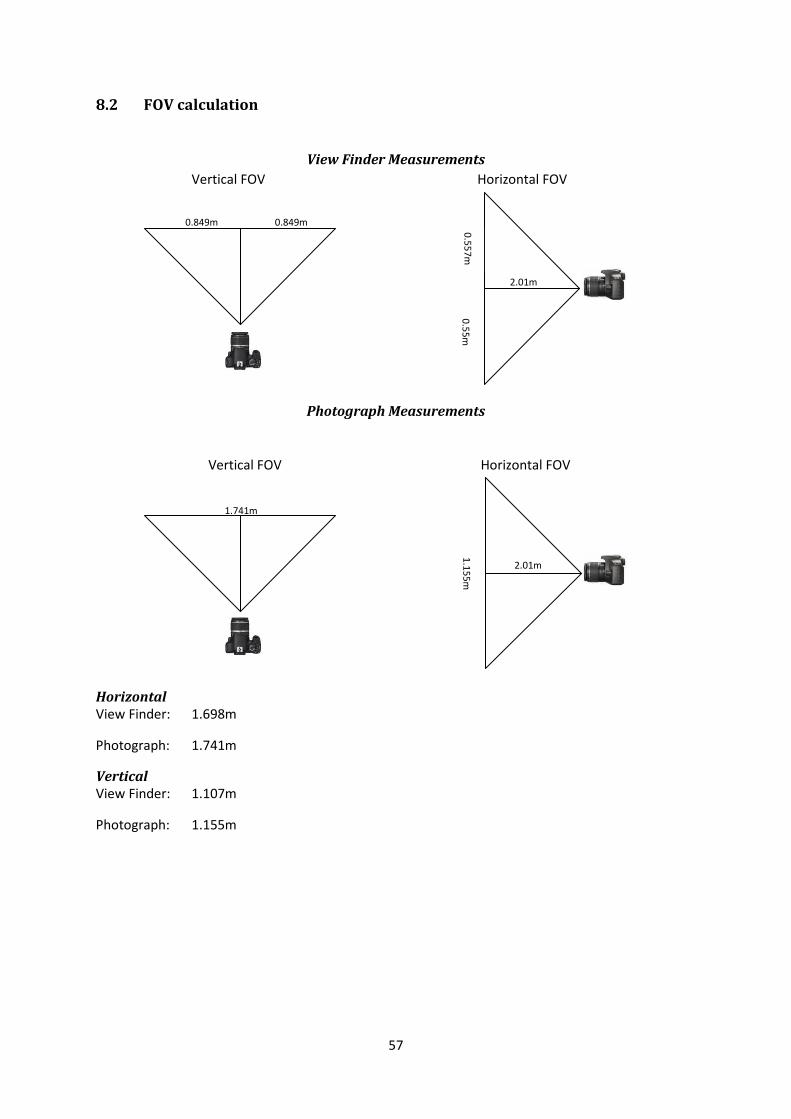
57
8.2 FOV calculation
View Finder Measurements
Vertical FOV Horizontal FOV
Photograph Measurements
Vertical FOV Horizontal FOV
Horizontal
View Finder: 1.698m
Photograph: 1.741m
Vertical
View Finder: 1.107m
Photograph: 1.155m
0.849m 0.849m
2.01m
0.5
57
m
2.01m
0.5
5m
1.741m
2.01m 1.1
55
m
2.01m
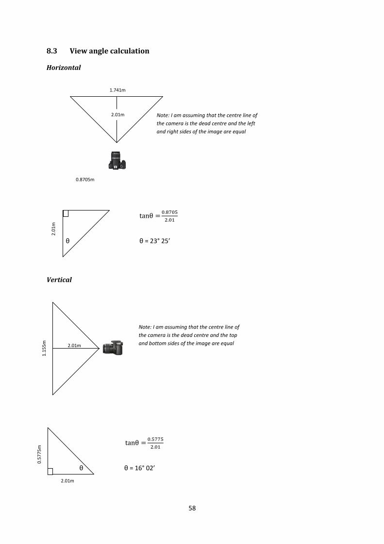
58
2.1m
8.3 View angle calculation
Horizontal
tanθ � �.�����.�
θ θ = 23° 25’
Vertical
tanθ � �.�����.�
θ θ = 16° 02’
1.741m
2.01m Note: I am assuming that the centre line of
the camera is the dead centre and the left
and right sides of the image are equal
0.8705m
2.0
1m
1.1
55
m
Note: I am assuming that the centre line of
the camera is the dead centre and the top
and bottom sides of the image are equal 2.01m
0.5
77
5m
2.01m