TRIHALOMETHANE FORMATION POTENTIAL IN THE SACRAMENTO … · THM formation potential test conditions (e.g., chlorine dose, temperature, reaction time, and pH) and by inorganic sources

TRIHALOMETHANE FORMATION POTENTIALIN THE

SACRAMENTO-SAN JOAQUIN DELTAMATHEMATICAL MODEL DEVELOPMENT

October 1991

State of CaliforniaThe Resources AgencyDepartment of Water ResourcesDivision of Planning

C-035901

State of CaliforniaThe Resources Agency

DEPARTMENT OF WATER RESOURCESDivision of Planning

Trihalomethane FormationPotential in the

Sacramento-San Joaquin Delta

Mathematical Model

DevelopmentOctober 1991

t Douglas R Wheeler Pete Wilson David N. KennedySecretary for Resources Governor Director

,ii~ The Resources Agency State .of California Department of Water Resources~r

Single cgpies of this report may be obtained withoutcharge. Additional copies are available for $2.00 eachand may be ordered from:

State of CaliforniaDEPARTMENT OF WATER RESOURCESP.O. Box 942836Sacramento, CA 94236-0~1

California residents add current sales tax.

C--035903(3-035903

FOREWORD

The Sacramento-San Joaquin Delta is a source of drinking water for 20 million Californians. Formation ofdisinfection byproducts known as trihalomethanes, or THMs, is promoted by organic matter and bromidesalts found in the Delta. Because these disinfection byproducts are a suspected threat to human healthwhen present at sufficient levels, the Environmental Protection Agency has established a standard of 0.1milligrams per liter for THMs in drinking water.

Two reports covering the Department of Water Resources’ Delta THM precursor monitoring program havebeen previously published. The In:st is titled The Delta as a Source of Drinking Water;, Monitoring Results, 1983to 1987; the second is titled Delta lsland Drainage Investigation Report of the Interagency Health AspectsMonitoring Program, A Summary of Observations During Consecutive Dry Year Conditions, Water Years 1987 and1988. Both reports are available from the Department.

This report documents the Division of Plarming’s first attempt to mathematically describe THM precursorsin the Sacramento-San Joaquin Delta. The model developed in this report, designed to simulate fate andmovement of THM precursors and to simulate THM formation potential chemistry, will ultimately be usedby the Division as a water quality planning tool. The present formulation has two important limitations.First, the model addresses Delta water quality and not tap water quality. This limitation exists because arelationship between THM formation potential and THMs at the consumer’s tap has not been clearlydefined for Delta water. Second, the model’s ability to assess agricultur, al impacts on Delta water quality islimited by available drainage site data. No conclusion should be drawn from the model results presented inthis report as the formulation is still preliminary.

Edward E Huntley~-’-~-~Chief, Division of Planning

C--035904C-035904

blank page - do not print

C--035905C-035905

CONTENTS

Page

FOREWORD ..............................................................................

ORGANIZATION, DEPARTMENT OF WATER RESOURCES ..................................... xi

ACKNOWLEDGMENTS .................................................................... xii

1 SUMMARY’Background ............~ .................................................................. 1Purpose and Scope ........................................................................1

Development ..............................................., ......... . .............Model 1Model Verification ........................................................................Model Application ......................................................................... 2Future Directions .......................................................................... 2

2 TRIHALOMETHANE FORMATION POTENTIAL ............................................ 3Chemistx~ of THM Formation ..............................................................3THM Regulations: Existing and Proposed ...........~ ....................................... 3THM Formation Potential Test ..............................................................3

3 THM PRECURSORS: ORGANIC MATTER ........... ........................................ 5Characteristics of Organic THM Precursors ...................................................5

Channel and Drain Characteristics ........................................................Delta Island Soil Characteristics ..........................................................Conservative Characteristics ...........................................................5

Sources of Organic THM Precursors .........................................................Summary of Previous MWQI Data Analyses ................................................. :. 7

Spatial Variation in THMFP .......~. ..................................................... 7Temporal Variation in THMFP ......................

4 THM PRECURSORS: BROMIDE ........................................................... 9Chemistry of Bromomethane Formation .....~ ...................................... , .......... 9 ¯Sources of Bromide..., .....................................................................9Significance of Bromide in THM Formation . ...................................................9Summary of Previous MWQI Data Analyses . .................................................9

C--035906C-035906

Page

Electrical Conductivity and TBFP Correlation ...............................................9Bromide and Chloride Correlation ........................................................9Effects of Hydrologic Conditions on TBFP ................................................10

OVERVIEW OF THMFP MODEL FORMULATION .......................................... ,11Motivation and Purpose ..................................................................11Literature Review of THM Formation Models ................................................11Conceptual Framework ...................................................................12Parameter Selection ......................................................................14

Precursor Effects .....................................................................14Bromide Effects ...................................................................... 16

Assumptions ........................... 16Limitations .............................................................................,17

DWR Delta Simulation Model .............................................................19DWRDSM Hydrodynamics ............................................................. 19DWRDSM Water Quality ~ .............................................................19

DWRDSM Calibration ...................................................................21Hand Adjustment Method ............................... ............................21Automated Method " . .............. ... " 21

Fate and Movement of THM Precursors with DWRDSM ......................................21Modes of DWRDSM Application.. .........................................................22

7 MODELING BROMINE INCORPORATION IN THM SPECIES ............................... 23Purpose ................................................................................ 23Bromine Incorporation Factor .............................................................23

Effects of Initial Conditions .................................; .......................... 23

Spatial Variation ...................................................................... 31 ~Bromine Distribution Factors ............ ................................................... 31Model Verification ....................................................................... 36

~:~ii:’

Internal Verification ................................................................... 36 ~:,~External Verification ..................................................................39

Example Problem ....................................................................... 42

8 APPLICATION OF THE THMFP MODEL .................................................. 45Modeling Objectives ...............~ ..................................................... 45Modeling Scenarios ................; ..................................................... 45ModeIing Assumptions ...................................................................48Results ............................~ .................................................... 49

Scenario 1 ................... " .......................................... 49

Scenario 2 ........................................................................... 49

C--035907C-035907

Page

Scenario 3 ........................................................................... 49Scenado 4 ........................................................................... 54Scenario 5 ........................................................................... 54Scenario 6 ........................................................................... 54Scenario 7 ......................... 60

Comparison with Historic Data ’ . ....................... ¯ ........60

9 FUTURE DIRECTIONS 65Enhanced Boundary Conditions ...........................................................65

Agricultural Drain Boundary Conditions " 65Other Boundary Conditions ............................................................67

Correlations Between THlVIFP and Actual THM Formation ...................................69Multi-Constituent Transport ..............................................................75Coordinated Data Collection and Analyses ..................................................75Management Alternatives Evaluation ......................................................75

Hypothetical Problem Definition ........................................................Hypothetical Problem Assumption ......................................................75Marginal Benefit Calculations ................................................; .........75

THMFP Reduction Calculations .............. " 79

REFERENCES ............................................................................. 81

APPENDIX A - REVIEW OF. DWR’S THMFP MODEL - G. AMY ................................. 85APPENDIX B - ESTIMATING TFPC AND CHLORIDE BOUNDARY CONDITIONS ................. 91

Sacramento River at Greene’s Landing ......................................................92Bay-Delta Interface at Benicia .......................¯ ...................................... 94

APPENDIX C - NOTATION 99

C 035908C-035908

FIGURES r

1. Composition and Distribution of Delta Soils .................................................6

2. Model Boundary Conditions and Output .............................¯ ...................... 13

3. THMFP versus TOC at Greene’s Landing .................................................15

4, THMFP versus TOC at Vernalis ...........................................................

5. DWRDSM Delta Model Grid ............................................................20

6, Bromine Incorporation Factor: Mathematical Definition ....... ........................... ....24

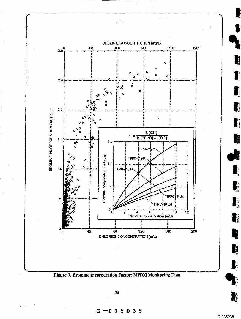
7. Bromine Incorporation Factor: MWQI Monitoring Data ......................................26

8, Bromine Incorporation Factor Submodels #1-~4:3-5 p,M TFPC Data Set .......................28

9. b as a Function of TFPC .................................................................30

10. Bromine Incorporation Factor: Submodel #5 ...............................................32,

11. Bromine Incorporation Factor: Observed versus Predicted Values .. ; ...........................33

12. Bromine Incorporation Factor at Export Stations .........................." ..................34

13. Bromine Incorporation Factor at Boundary Stations .................................." .......35

14, Bromine Distribution Factors .................................... 37

15. Bromine Distribution Factor~: Observed versus Predicted Values ...............................38

16, Bromine Incorporation Factor Verification .................................................40

17. Bromine Distribution Factors Verification ..................................................41

18. THMFP Model Methodology: Example Problem ..................................~ .........43

19. Net Flow Directions: July 1988 Model Scenarios .............................................

20. Sacramento River TFPC Impact: Scenario 1 (TFPC in

21. San Joaquin River TFPC Impact: Scenario 2 (TFPC in gg/L) ..................................52

22. Bay TFPC Impact: Scenario 3 (TFPC in ~tg/L) ..............................................53

23. ~_Peat Drainage TFPC Impact: Scenario 4 (TFPC in I.tg/L) .....................................

24. Mineral Drainage TFPC Impact: Scenario 5 (TFPC in ~tg/L) ..................................56

25. Cumulative Source TFPC Impact: Scenario 6 (TFPC in/.tg/L) .................................

26. TFPC at Clifton Court Forebay: Scenario 6 .................................................58

27. TFPC at Selected MWQI Monitoring Stations: Scenario 6 ....................................59

28. Cumulative Source Salinity Impact: Scenario 7 (TDS in rag/L) .................................61

29. Field and Model Values: THMFP Steady State Analysis ......................................62

30. TFPC Contributions from Agricultural Drainage ............................................66

C--035909(3-035909

Page

31. Boundary Conditions at Vemalis .......................................................... 68

32. Flow-TFPC Relationship at Vernalis ......................................................70

33. Banks Pumping Plant SDS Tests ..........................................................71

34. THMFP Data Adjusted to SDS Conditions ’ . ............................... 72

35. Source Water DBP Study ................................................................73

36. Other SDS Studies ..................................................................... 74

37a. Marginal Benefits of Bromide Control .....................................................76

3To. Marginal Benefits of Bromide Control. ....................................................77

B-1. Boundary Conditions at Greene’s Landing .................................................93

B-2. Flow-TFPC Relationship at Greene’s Landing .........’ ..................................... 95

B-3. Boundary Conditions at Mallard Island ....................................................96

B-4. Chloride-TFPC Relationship at Mallard Island .............................................98

ix

�-o3591 oC-035910

TABLES

1. Initial Screening: Bromine Incorporation Factor Submodels ....................................:~7

2. Modified Submodel #2: Further Screening Analysis ..........................................29

3. Peat Island Discharge Distn’bution, Scenario 4 .............................................46

4. Mineral Island Discharge Distribution, Scenario 5 .............................

5. July 1988 Boundary Conditions Using DWRDSM ~ . .......48

6. TI-IMFP: Base versus Plan Conditions .......... " 79

C--035911C-035911

ORGANIZATION ¯

STATE OF CALIFORNIAPete Wilson, Governor

THE RESOURCES AGENCYDouglas R Wheeler, Secretary for Resources

DEPARTMENT OF WATER RESOURCESDavid N. Kennedy, Director

John J. Silveira Robert G. Potter James U. McDanielDeputy Director Deputy Director Deputy Director

L. Lu6inda Chipponefi Susan N. WeberAssistant Director for Legislation Chief Counsel

Division Of Planning

Edward F. Huntley ........, .................................................................. Chief

George W. Barnes, Jr .................................................Chief, Modeling Support Branch

This report was prepared under the supervision of

Francis Chung ................................................................Supervising EngineerAli Ghorbanzadeh Senior Engineer

Paul Hutton ....................................................................Associate Engineer

with assistance from

Sam Ito ..................................................................... Engineering AssociateNancy Daddona ................................................................Editorial Technician

C--03591 2C-035912

ACKNOWLEDGMENTS

The valuable assistance provided by the many persons who contn"outed information and ideas to this report isgratefully acknowledged. Special thanks go to Stuart Krasner of The Metropolitan Water District ofSouthern California; Rick Woodard and Bruce Agee of the Department of Water Resources’ Division ofLocal Assistance; Marvin Jung of Jung and Associates; Gary L Amy, Professor of EnvironmentalEngineering, University of Colorado at Boulder; and James M. Symons, Consultant.

The Technical Advisory Group of the Municipal Water Quality Investigations Program also providedtechnical assistance in preparing this report. Member agencies of the Technical Advisory Group included:

California Department of Health ServicesCalifornia State Water Resources Control BoardCalifornia Urban Water AgenciesContra Costa Water DistrictEast Bay Municipal Water DistrictUrban Water Contractors of the State Water Project including:.

Alameda County Flood Control and Water Conservation District, Zone 7Alameda County Water DistrictLos Angeles Department of Water and PowerMetropolitan Water District of Southern CaliforniaSanta Clara Valley Water District

U.S. Environmental Protection Agency

C--03591 3C-035913

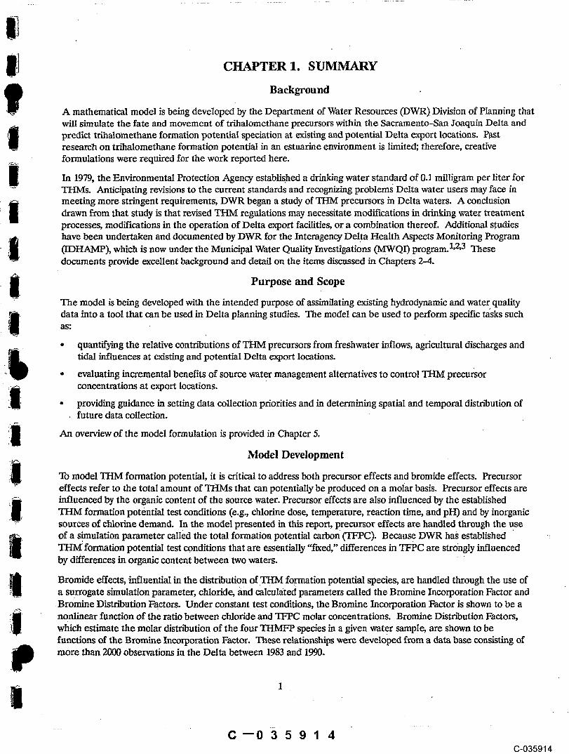
CHAPTER 1. SUMMARY

Background

A mathematical model is being developed by the Department of Water Resources (DWR) Division of Planning thatwill simulate the fate and movement of trihalomcthane precursors within the Sacramento-San Joaquin Delta andpredict trihalomethane formation potential speciation at existing and potential Delta export locations. P.astresearch on trihalomethane formation potential in an estuarine environment is limited; therefore, creativeformulations were required for the work reported here.

In 1979, the Environmental Protection Agency established a drinking water standard of 0.1 milligram per liter forTHMs. Anticipating revisions to the current standards and recognizing problems Delta water users may face inmeeting more stringent requirements, DWR began a study of THM precursors in Delta waters. A conclusiondrawn from that study is that revised THM regulations may necessitate modifications in drinking water treatmentprocesses, modifications in the operation of Delta export facilities, or a combination thereof. Additional s.tudieshave been undertaken and documented by DWR for the Interagency Del.ta Health Aspects Monitoring Program(IDI-IAMP), which is now under the Municipal Water Quality Investigations (MWQI) program.1,2,3 Thesedocuments provide excellent background and detail on the items discussed in Chapters 2-4.

Purpose and Scope

The model is being developed with the intended purpose of assimilating existing hydrodynamic and water, qualitydata into a tool that can be used in Delta planning studies. The model can be used to perform specific tasks suchas:

¯ quantifying the relative contn’butions of THM precursors from freshwater inflows, agricultural discharges andtidal influences at existing and potential Delta export locations.

o evaluating incremental benefits of source water management alternatives to control THM precursorconcentrations at export locations.

¯ providing guidance in setting data collection priorities and in determining spatial and temporal distribution offuture data collection.

An overview of the model formulation is provided in Chapter 5.

Model Development

To model THM formation potential, it is critical to address both precursor effects and bromide effects. Precursoreffects refer to the total amount of THMs that can potentially be produced on a molar basis. Precursor effects areinfluenced by the organic content of the source water. Precursor effects are also influenced by the establishedTHM formation potential test conditions (e.g., chlorine dose, temperature, reaction time, and pH) and by inorganicsources of chlorine demand. In the model presented in this report, precursor effects are handled through the useof a simulation parameter called the total formation potential carbon OWPC). Because DWR has establishedTHM.formation potential test conditions that are essentially "fixed," differences in TFPC are strongly influencedby differences in organic content between two waters.

Bromide effects, influential in the distribution of.TI-IM fo..rmation potential species, are handled through the use ofa surrogate simulation parameter, chloride, and calculated parameters called the Bromine Incorporation Factor andBromine Distn"oution Factors. Under constant test conditions, the Bromine Incorporation Factor is shown to be anonlinear function of the ratio between chloride and TFPC molar concentrations. Bromine Distribution Factors,which estimate the molar distn"oution of the four THMFP species in a given water sample, are shown to befunctions of the Bromine Incorporation Factor. These relationships x~ere developed from a data base consisting ofmore than 2000 observations in the Delta between 1983 and 1990.

C--03591 4C-035914

An existing numerical hydrodynamics and water constituent transport model is used to mimic the fate andmovement of precursor and bromide parameters from the upstream model boundaries to the downstream exportlocations. Used within the framework developed in this report, the transport model can be used to answer thefollowing generalized question: Given certain precursor and bromide effects at the upstream model boundaries(e.g.. Sacramento River at Greene’s Landing, San Joaquin River at Vernalis, Bay-Delta interface at Benicia,agricultural drainage locations, and minor fresh water tributary inflows), what are the precursor concentrations,bromide concentrations and the resulting THM formation potential species distributions at Delta export stations?The numerical transport model and development of the overall THM formation potential model framework arediscussed in Chapters 6 and 7.

Model ~Verification

The Bromine Incorporation Factor and Bromine Distribution Factor relationships were verified both internally andwith an external data set of 1025 observations. The Bromine Incorporation Factor submodel was verified against asubset of the external data base (64 observations) that more or less represents DWR’s THM formation potentialtest conditions. This data subset has constant reaction times of 168 hours and reaction temperature of 20°C. Whilethe verification shows a good correlation between predicted and observed values, it also indicates that ~he submodeltends to overpredict at low values of the factor and to underpredict at high values of the factor. The difference inchlorine dose between the external data base and the dose utilized in DWR’s test is a likely explanation for themodel underprediction at high values of Bromine Incorporation Factor. Variability in other test conditions may alsoexplain some of the deviation between model predictions and observed values.

The Bromine Distn’bution Factor relationships were verified against the entire external data set. The external database follows the submodel relationships as well or better than the internal data base. This comparison shows thatTHM formation potential species distribute in a predictable fashion under varying test conditions° Modelverification is presented in Chapter 7.

Model Application

Seven transport simulations were performed to illustrate potential model utility in meeting the following objectives:to quantify individual and cumulative impacts of THM precursor sources at Delta export locations and to simulatebromide effects at Delta export locations. Each simulation assumed historic hydrologic and water quality boundaryconditions (July 1988) and each was performed in a steady state mode. Steady state mode was selected to simplifythe analysis and was considered to be appropriate for illustrative purposes. Because of this and other simplifyingassumptions associated with the simulations, no conclusions should be drawn from the preliminary model resultspresented in thls report.

Conceptually, model utility in quantifying precursor impacts and bromide effects in the Delta was illustrated by thesimulations. Model results were compared with historically observed values at seven locations in the Delta,including four export locations. Model results compared favorably with observed values at three of the four exportstations (Clifton Court Forebay, Delta-Mendota Canal.at Tracy Pumping Plant and Contra Costa Canal at RockSlough). A less favo~ablemodel result at North Bay Aqueduct at Lindsey Slough was attn"outed to aninappropriate water quality boundary condition assignment for the Y01o Bypass. It was observed that agriculturaldrainage was influential at stations where model deviations were the greatest, thereby highlighting a need to moreaccurately descn~oe agdctiltural drainage quality and quantity in the Delta. Model application is presented inChapter 8.

Future Directions

Future directions in THM formation potential model development are discussed in Chapter 9. Areas identified forfuture enhancement include but are not limited to: developing an algorithm that descn’bes THM precursorcontributions from agricultural drainage; refining boundary conditions at Delta inflow locations;, and definingrelationships between TI-IM formation potential, as measured in source waters, and THM concentrations in treateddrinking water.

2

C--03591 5(3-035915

CHAPTER 2. TRIHALOMETHANE FORMATION POTENTIAL

Chemistry of THM Formation

Public drinking water supplies are typically disinfected prior to distnqgution to consumers. Free chlorination is thepredominant method of disinfection in water treatment practice. Although free chlorination provides a water safefrom bacteriological contamination, it allows for the formation of several chemical by-products. TrihalomethanesO"HMs) are one group of disinfection by-products formed when soluble organics are oxidized by free chlorine.THM compounds include: chloroform (CHCI3), dichlorobromomethane (CHC12Br), d~romochloromethane(CHCIBr2), and bromoform (CHBr3).

During disinfection, molecular chlorine reacts with water by the following reversible reactiqns:

Cl2(aq) + H20 +-~ HOCI + H+ + CI- . ......................................................... (2-1)

HOC1 ~-+ H+ + OC1- . ....................................................................... (2-2)

The relative amounts of hypochlorous acid (HOCI) and hypochlorite (OCI-) produced in the above reactions are afunction of pH. These chlorine species, known as free chlorine, are the disinfecting agents in the chlorinationprocess. Free chlorine reacts with soluble organics to form THM compounds by the following reaction:

Organics + Free Chlorine -+ THMs + Other Disinfection By-Products ..............................(2-3)

If bromide is not present, chloroform is the only THM formed. If present, it competes with free chlorine to formbrominated THM species, also known as bromomethanes. The chemical mechanism of THM formation in thepresence of bromide is discussed in Chapter 4.

THM Regulations: Existing and Proposed

Currently, water utilities must reduce the total concentration of TI-LMs to 0.10 mg/L to meet state and federaldrinking water standards. This Maximum Contaminant Level (MCL) was not established strictly on the basis ofhealth effects data but was set as a feas~le level for compliance by water utilities. A lower MCL is beingconsidered by the Environmental Protection Agency for human health protection.1 The THM standard applies todrinking water in the distribution system, not at the source.

THM Formation Potential Test

In 1981 DWR developed a THM Formation Potential (THMFP) test to compare THM producing capacities ofdifferent Delta inflows and outflows. The .THMFP test requires a high dose of chlorine to meet the chlorinedemand of suspended and organic material in the samples and to maintain a chlorine residual during the holdingperiod. While the test conditions do not reflect actual water treatment conditions, the IDHAMP TechnicalAdvisory Group found the procedure acceptable for the purposes of comparing relative levels of THM precursorsin Delta ~vaters.1

In this procedure, THMFP samples are spiked with a dosage of 120 mg/L of chlorine, a concentration sufficientlyhigh to meet the highest chlorine demand and maintain a residual after incubation at 25°C for seven days.. EarlierDWR results showed this high chlorine dose was necessary for meeting the exceptionally high chlorine demandtypically found in agricultural drain water samples, pH is not standardized in the test procedure. At the end of theincubation period, samples are dechlorinated and analyzed for THM compounds by the gas chromatograph purgeand trap method.

A direct relationship between the THMFP test results and THM production under ac.tual treatment conditions hasnot yet been developed. However, the amount of THMs formed during normal disinfection is influenced by theamount of precursor materials available. Therefore, a source water with high THMFP is generally indicative of awater that will contain high THM concentrations upon water treatment.

C--03591 6C-035916


|~

4

C--03591 7C-035917

Characteristics of Organic THM Precursors

As shover in Eq. 2-3, organics are the primary precursor in THM formation. Humic substances are generallyconsidered to be the most important organic THM precursor in natural waters. Humic substances, which includehumie and fulvie acids, are an extremely complex and diverse group of organic materials whose structure is not welldefined. They are a mixture of poorly biodegradable decomposition products and by-products of natural organicmatter produced by both plants and animals.4 Because of the variability of humic substances, formation of TH_Msmay vary with the different origins and properties of the humic substance.1

Channel and Drain Characteristics

et al.5 concluded that the THM in Delta channel and drain waterAmy organic precursors agricultural samplesaresignificantly different in their character and propensity to form THMs. Organic matter in drain water was found tobe more reactive and to have greater molecular sizethan organic matter in channel water in.forming THMs.Because of these differences in reactivity and molecular size, concentrating effects of applied water has beendiscounted as the primary explanation for the high THMFP found in agricultural drains. Soil leaching is consideredto be the dominant process that transports organic precursors into the drains,t

Delta Island Soil Characteristics

Delta islands are maior storage pools of humic substances due to underlying organic softs. Delta soft types havebeen grouped into three broad classes: mineral, intermediate organic, and peaty organic.6 All three soft typescontain organic matter, with mineral, softs tile least am~aunt (less than 10 percent) and peaty organic softs the most(50 to 80 percent).. The composition and distdbution of Delta softs is depicted in Fig. 1. Tests have showncomposited Delta mineral and peat soil extracts to have THMFP values in the range of 27,000 gg/kg and 61,000gg/kg, respectively.7 This difference between softs indicates that THMFP is related to soil type and watersaturation of the island soils.I

Conservative Characteristics

Dissolved organics have been observed to behave conservatively in rWaters with salinity less than 5000 mg/L,8,9,10,11,12 the range generally found in the Delta. Humie substances, the most reactive organic fraction in formingTHMs, are very resistant to natural biological degradation and tend to precipitate from solution only underextremely saline conditions.13 Organic THM precursors can be treated as conservative constituents in Delta watersnot because of low salinities, but also because of shortresidence times. With the of fewonly water exception asloughs, Delta inflows are generally transported to export pumps or out into the bay in a few days or weeks.1

~ Sources of Organic THM Precursors

Delta waters receive.0rganic materials from a variety of sources, including: agricultural drainage, Stlrfaee runoff,wastewater treatment plant discharges, algal productivity, in-channel softs, levee materials, and riparian vegetation.Organic THM precursor contn~outions from agricultural drainage is currently under intense study. Results indicatethat, in terms of concentration, agricultural drainage is ~a significant precursor source.1 Preliminary studies byDWR have shown urban storm water runoff to have THMFP concentrations similar to those of agricultural drains,2

whereas effluent from wastewater treatment plants does not appear to be a significant source of precursors in theDelta.1 DWR has recommended that studies be undertaken to determine the impact of algal productivity onTHMFP"3

5

C--03591 8(3-035918


,|

C--03591 9C-035919

CHAPTER 4. THM PRECURSORS: BROMIDE

Chemistry of Bromomethane Formation

When water containing bromide ion is chlorinated, the bromide is oxidized to hypobromous acid according to thefollowing reaction:

Br- + HOCI --~ HOBr + CI-. ...................................................................(4-1)

Hypobromous acid competes with free chlorine to produce THMs according to the general reaction:

Organics + HOCI + HOBr -~ THMs + Other Disinfection By-products .............................(4-2)

If bromide is absent, chloroforrn (CHC13) is the only THM species produced in the above reaction. But if bromideis present during this reaction, the following bromomethanes are also produced: dichlorobromomethane(CHC!2Br), dibromochloromethane (CHCIBr2) and bromoform (CHBr3).

Sources of Bromide

The major sources of bromide in the Delta are from sea water intrusion, agricultural drain discharges, and the SanJoaquin River.2 Connate waters are another source of bromide and may be significant in certain locations of theDelta.1 ~

Significance of Bromide In THM Formation

Researchers have shown that molar yields of THMs increase with increasing bromide concentration.16,17,18Furthermore, THM speciation~has been observed to shift toward the heavier bromomethanes as the concentrationof bromide increases.19 Because the atomic weight of bromine is heavier than that of chlorine (79~91 versus 35.45),the molecular weight of bromomethanes increase in proportion to the number of bromine atoms present: CHCI3[119.36], CHC12Br [163.82], CHC1Br2 [208.28], and CI-IBr3 [252.74]. Therefore, bromide not only increases theextent of THM formation on a molar basis, bromide also increases the extent of THM formation on a molecularweight basis. In addition to these problems, bromomethanes can complicate THM treatment processes and thehealth risks associated with bromomethanes may be greater than those of chloroform.

Summary MWQI Analysesof Previous Data

DWR has documented a number of observations related to Total Bromomethane Formation Potential (TBFP)based on THM data collected in the Delta.1,2,3 TBFP was delrmed as th~ sum concentration of the threebromomethanes, i.e. CHC12Br, CHCIBr2, and CHBr3.

Electrical Conductivity and TBFP Correlation

Simple linear relationships were investigated between electrical conductivity (EC) and TBFP for channels anddrains on a Delta-wide scale. These correlations were poorly defined, with coefficients of determination (r2) of0.66 and 0.54, respectively. Linear relationships were also investigated at individual monitoring stations.Correlations varied greatly by location; only three of twelve stations had r2 values greater than 0.80. Based onthese results, DWR concluded that inorganic constituents have a strong effect on TBFP at some stations; however,the use of EC, chloride, or TDS to predict TBFP on a Delta-wide scale is not appropriate because of poorcorrelation. It has been suggested that a multivariate analysis would reveal stronger relationships between EC andTBFP in the Delta.20

Bromide and Chloride Correlation ’

Because typical concentrations of bromide and chloride in open ocean water are about 65 mg/L and 19,000 rag/L,respectively,4 the following relationship would be expected based solely on sea water intrusion:

C--035920(3-035920

THM = THM concentration, ttMBr- = bromide concentration, mg/LC12 = chlorine dose, mg/LT = temperature, °CTOC. --- nonvolatile total organic carbon, mg/Lb0,bl,b2,b3,b4,b5 ---- model coefficients

Amy et al.28 applied the Morrow and Minear model to additional data sets. Amy, Chadik, and Chowdhury29studied the effect of chlorination on nine natural waters located throughout the United States. From a set of 995observations, the following multiple regression model was developed:

THM ---- bo (UVA x TOC)bl (Cl2)b2 (t)b3 (T)b4 (pH-2.6)b5 (Br- + 1)b6 .................................(5-3)

Where:THM ----- THM concentration,UVA --- absorbance of ultraviolet light at a wavelength of 254 nm, cm-1TOC --- total organic carbon, mg/LC12 -- chlorine dose, mg/Lt -- reaction time, hrsT = temperature, oCBr- -- bromide concentration, mg/Lb0,bl,b2,b3,bg,bs,b6 = model coefficients

The authors investigated a number of potential organic precursor parameters, including: TOC, UVA, relativefluorescence, and color. Statistically, the best overall organic precursor parameter for predicting THM was themultiple.term (UVA x TOC). The chemical significance of this term is that TOC defines the precursorconcentration while UVA defines the precursor reactivity in forming THIVIs.

Regression analysis indicted that THM formation theoretically commenced at pH 2.6 for the nine waters studied,therefore the parameter (pH -2.6) was utilized. Urano et a126 found that chloroform formation commenced at pH2.8. Natural bromide concentrations ranged from 0.010 - 0.245 mg/L; however, samples were spiked to increase themaximum value to 1.245 mg/L. The authors indicated that the bromide term can be deleted from the model withonly a small loss of predictive accuracy. Other THM models have also been proposed.30,31,32

Past research on THM formation potential in estuarine or bromide-rich environments is limited. As a result, manyof the previous modeling efforts do not consider bromide effects in THM formation and speciation. Also, asrevealed in the literature, a typical objective of existing models is to evaluate finished water, managementalternative.s through the description of THM reaction kinetics. Because this study is concerned with evaluatingsource water management alternatives in a bromide-rich environment, site-specific data and innovativeformulations were essential in developing a model of the Sacramento-San Joaquin Delta to simulate raw waterTHM formation potential and speciation.

Conceptual Framework

The THMFP model is conceptually divided into two main components, 1) simulation of THM precursor transportand 2) simulation of THMFP species distribution. These components are addressed in detail in Chapters 6 and 7.

Fig. 2 illustrates the model flow logic and interaction between each model component. The purpose of thetransport component is to determine THM precursor concentrations at existing and proposed export stations fromknown boundary conditions° Boundary conditions (transport model inputs) are denoted in the figure by a "B."Export water qualities (transport model outputs) are denoted in the figure by a "E." The objective of the THMFPdistnqaution simulation component is to estimate concentrations of CHCI3, CHC12Br, CHCIBr2, and CHBr3 that

12

C--035921(3-035921

SACRAMENTO RIVER

®DELTA

EXPORTS

Rio Vista

SUISUN MARSHSAN FRANCISCO BAY

DELTAEXPORTS

® ® CHCI3Delta Exports 120 mg/L CI2= CHCI2 BrTHM Precursors 25° C, 7 days CHCI Br2 = THMFP

CHBr3

(~ Model input - Plan/Historic Conditions

I~ Model Output

(~)’fI-IMFP = f (TFPC, Br’) DELTATracy ¯

EXPORTS (~SAN JOAQUIN

RIVER

Figure 2. Model Boundary Conditions and Output

C--035922C-035922

would be produced by a water sample under DWR’s test conditions, assuming export water quality determined inthe transport component. Simulation of THMFP species distnqgution is denoted by a "D" in Fig. 2. For example,given certain precursor concentrations at the model boundaries (e.g., Sacramento River at Greene’s Landing, SanJoaquin River at Vernalis, Bay-Delta interface at Benicia, agricultural drainage locations), what are the precursorconcentrations and resulting THMFP species distributions at Delta export stations?

Parameter Selection

To model THMFP, it is critical to address both precursor effects and bromide effects. Precursor effects influencethe total amount of THMs that are produced on a molar basis. Precursor effects are related to the organic contentof the source water and are also related to the conditions established for the THMFP test. Bromide effects areinfluential in the distribution of species formed in the THMFP test. Bromide effects are related to ambientbromide concentration, organic content, and to established THMFP test conditions. Therefore, to model THMFP,parameters must be selected to represent organics, bromide, and THMFP test conditions.

Precursor Effects

Chlorine dose, reaction time, temperature and pH are identified in Eq. 5-3 as important parameters that describeprecursor effects related to THMFP test conditions. Chlorine residual, another important parameter, wasmaintained relatively constant by Amy et al.29 with a 3:1 chlorine to TOC ratio. Because chlorine dose, reactiontime and temperature are "fixed" in DWR’s THMFP test, it was not necessary to explicitly include theseparameters in a description of precursor effects. Chlorine residual and pH, on the other hand, are allowed to varyin DWR’s THMFP test. But as data is not generally available for these remaining test condition parameters(chlorine residual data has been collected in recent years), chlorine residual and pH were also excluded from aprecursor effects description.

TOC is identified in Eq. 5-3 and generally throughout the literature as an important parameter that describesprecursor effects related to organic matter. If all natural organic matter readily reacted with free chlorine to formTHMs, then TOC or dissolved organic carbon (DOC) would be direct indicators of organic THM precursors. Notall organic compounds found in water are THM precursors, however. Good correlations have been obtainedbetween TOC and DOC and THM’FP for single water sources,5,15,33,34 but when waters from different sources areincluded in a single comparison, the correlations are Sometimes not as good~35 This is because TOC and DOC tendto contain variable mixtures of organic matter that are active in forming THMs, the mixture being dependent onthe source’s particular watershed characteristics.

DWI~ has found very few dearly defined relationships between TOC or DOC and THMFP in Delta source waters.Figs. 3 and 4 illustrate the poor correlations in the Sacramento River at Greene’s Landing and in the San JoaquinRiver at Vernalis. Elimination of a few outlying points does not improve the relationships significantly. Removingfour outliers at Greene’s Landing (Fig. 3) increases the r2 value to 0.35. Removing one outlier at Vernalis (Fig. 4)increases the r2 value to 0.17.

Specific formation potentials are nearly identical for the two Delta tn~outaries. The average specific THMFP atGreene’s Landing is 133 Ixg/mg TOC; the average specific THMFP at Vemalis is 131/xg/mg TOC. Individualvalues at both locations are highly variable, however, with standard deviations of 57 ttg/mg at Greene’s Landing and51 ~g/mg at Vernalis. Reckhow and Singer35 reported an average specific THMFP of 52 p.g/mg TOC from sevendifferent water sources. Differences in THMFP test conditions probably account for the discrepancy between thevalues reported by the researchers and DWR. The researchers utilized 20-60 mg/L chlorine doses and a three dayreaction time, compared with a 120 mg/L chlorine dose and seven day reaction time utilized by DWRo NeitherTC~C nor DOC was selected as a surrogate measure of precursor effects in the Delta because of the poor

¯ correlations discussed above.

14

C--035923C-035923

¯r2 = 0.19

400

:" ¯ "i.. " ," !, ~

¯200 .... : ............................. ~’:’: ........ o’; .................. "; ......................... :" ............................................... ": ................................................ : ....

O .... :" .................................................: ................................................:" ...............................................":- ....................................................1 "’ ’ " ! ~ ~ ’ I ’ * ~ I ~ ’ ’’ " I

TO(3

Figure 3. THMFP versus TOC at Greene’s Landing

1200 .................................................... : ............................ ; ........................................................................................................................*:

:: r2 = 0.09 -:¯e~ .... i ....................................:"" ...........................................................................: ...........................................................i ...............~ ....

800 ............. : ................................. ’ ......

~ , ¯ .:

88° ....i ................................................i ...............; ........."- ........................’-.: ............~ .............................~ ....................................i .....

488 .... i ................................ .................. ;’""-"/ ................ v’~.-..; ...................................... ~.- ............................................... i ....

-288 ................................. ’ .............." ............................................... : ...............................................................................................

e .... : ................................................................................................................................................. -.’- ........... .................................... ~’"--1I , . .., , . ~ , ~ , , I . .. , .

TOC

Figure 4. THMFP versus TOC at Vernalis

C--0a5924C-0~5924

UVA is also identified in Eq. 5-3 and elsewhere in the literature15,33 as an indicator of organic THM precursors.UVA measurements permit the concentration of high molecular weight molecules (e.g. humic and fulvic acids) tobe assessed in a semiquantitative fashion. In this way, UVA is more selective for THM precursors than is TOC orDOC.36 UVA was not measured under the IVIWQI program until May 1990 and therefore was not selected as asurrogate measure of precursor effects in the Delta.

Research has shown that molar yields of THMs increase with increasing bromide concentration.16,17,18 However,Amy et al. found molar THMFP to be relatively insensitive to bromide concentration.29 Therefore, bromide wasnot selected as a parameter to describe precursor effects.

Given the above limitations of surrogate measures and given the overall model objectives, the TFPC parameter wasselected to simulate precursor effects in the Delta. Variation in TFPC is strongly indicative, of differences in theorganic content and organic reactivity of Delta waters, as DWR’s THMFP test conditions are essentially "fixed."(Granted, differences in pH and chlorine residual may also corttn’bute to varying TFPC values.) TFPC provides asingle common basis for quantifying the precursor effects in various source waters. In contrast, utilizing TOC,UVA, or a product of the two parameters to represent organic precursors requires a more sophisticated modelframework. Specifically, it would be necessary to model the fate and movement of additional water quality ¯parameters that descn’be the chlorine demand and activity of each source water. And even if strong multivariaterelationships were established, such a model would be much more complex to develop and cal~rate. Furthermore,the data required to develop and calibrate such a model is not currently available in sufficient quantities on aDelta-wide basis.

The TFPC parameter is calculated directly from measured THMFP data as follows:

¯ Divide the mass concentration of each THlVIFP compound by its respective molecular weight and sum the fourconcentrations to yield a molar concentration of THMFP. Since the molar ratio of THMFP to TFPC is 1:1, thisvalue is also the molar concentration of TFPC.

¯ To obtain a mass concentration of TFPC, multiply the molar concentration by 12, the atomic weight of carbon.

Bromide Effects

Bromide was not measured under the MWQI program until May 1990 and available data is limited. Therefore, adecision was made to utilize chloride as a surrogate measure of bromide in the Delta. By using chloride as arepresentative parameter of bromide effects, the model formulation implicitly assumes the ratio between these ionsis consistent throughout the Delta. The ionic ratio has been observed to be most consistent in the western Deltaand less consistent in agricultural drains and in the interior Delta where seawater intrusion is insignificant.Fortunately~ these latter areas have not generally demonstrated significant bromide effects (because of low ionicconcentrations and or high precursor concentrations),, thereby minimizing any potential discrepancies. Modelingbromide effects is discussed at length in Chapt.er 7. ’

Assumptions

Several key assumptions were made in developing the THMFP model formulation. These assumptions areoutlined below:.

1. Precursor effects in the Delta can be simulated through the use of the TFPC parameter. Bromide effects canbe simulated with a surrogate measure of bromide--chloride. The rationale for these assumptions is given in theabove section, "Parameter Selection."

2. Precursor and bromide effects are known at the model boundaries, i.e. TFPC and chloride concentrations arespecified as boundary conditions. Model boundaries include:

¯ Sacramento River at I Street Bridge° Water quality at this boundary is assumed to be identical with observed

16

C--035925C-035925

¯ San Joaquin River at Vernalis

¯ Cosumnes River

* Mokelumne River

¯ Yolo Bypass

* Other miscellaneous rivers and streams tributary to the Delta

¯ Bay-Delta interface at Benicia

¯ Agricultural drain sites

3. Fate and movement of TFPC and chloride within the Delta can be modeled with conservative constituentassumptions. The rationale for this assumption is discussed in Chapter 3.

4. Precursor effects are dependent only on the fate and movement of TFPC specified at model boundaries.Bromide effects are dependent on interactions between chloride (i.e. bromide) and TFPC at individual locations.

Limitations

Limitations of the THMFP model formulation are as follows:

1. A lack of flow and water quality data limits the ability of the model to assess TFPC contributions from"agricultural drainage. DWR previously recommended an expansion of the MWQI monitoring program to include alarger number of Delta island drains.1 Enhancing the boundary condition description at agricultural drains, asdiscussed in Chapter 9, will require additional data.

2. TFPC cannot be estimated a priori to predict THMFP; it must be calculated from historical THMFPmeasurements. Therefore, TFPC cannot be used as a parameter to model TI-IMFP in a predictive or real-timeoperations mode. However, with adequate historical data at bo~undary conditions, TFPC can be u~ed as asimulation parameter to model THMFP in a historical or planning mode. This limitation is not critical because theTHMFP model was designed as a planning tool with which various planning alternatives can be evaluated in anincremental, or comparative manner. Establishing multivariate relationships between TFPC and directlymeasurable water quality parameters to descnqge freshwater and Bay-Delta boundary conditions would permit themodel to be used in a predictive mode. This potential modal enhancement is identified as an area of futureresearch and is discussed further in Chapter 9.

3. Correlations have not been developed between DWR’s THMFP data and THM formation in a water treatmentsystem. The THMFP test conditions skew both the total and distribution of THMs formed relative to typical watertreatment conditions, producing more total "IT/Ms but smaller fractions of bromomethanes. While this fact limitsthe model’s applicability, the lack of an established correlation does not pr0h~it the model, from being used for itsintended purpose because a) source waters with high THMFPs tend to indicate waters that will produce high THMsduring water treatment, and b) the model evaluates source water management alternatives, not treatmentalternatives. Singer37 offered the following limitations generally associated with THMFP tests:

The principal limitation in the use of the THMFP concept is that it is not intended to be used as a predictive device fordetermining the concentration of THMs reaching the consumers’ tap. It is a measure of the precursor content of agiven wat~...Nevertheless, it may be possible for a utility to develop its own predictive model provided a suitable database can be established for the specific treatment and hydraulic, conditions for that utility.

Developing Correlations between raw water THMFP and finished water THMs was previously identified as an areaof future research1,38 and is discussed further in Chapter 9.

-13"035926(3-035926

CHAPTER 6. MODELING FATE AND MOVEMENT OF THM PRECURSORS

DWR Delta Simulation Model

DWR has developed a numerical~ model to simulate hydrodynamics and water quality within the Sacramento-SanJoaquin Delta. The model, called DWR Delta Simulation.Model (DWRDSM), simulates flow, stage, velocity, andconservative water constituents at various locations in the Delta for a given hydrology and channel geometry.DWRDSM is an enhanced version of the Fisher Delta Model.39,4° Solution schemes employed by the model arethe Method of Characteristics and the Lagrangian Method for hydrodynamics and water quality, respectively. Themodel includes approximately 500 nodes, 600 channels and 13 open reservoirs or lakes. Fig. 5 shows a networkrepresentation of the Sacramento--San Joaquin Delta as used in DWRDSM. To simulate Delta hydrodynamics,flows are specified at the upstream boundaries and tidal stages are specified at the downstream boundary (Benicia).Export pumping demands and Delta consumptive use are also specified. To simulate water quality, concentrationsare specified at all boundaries.

The transport model has been used by DWR to quantify the effects of levee breaks, changes in net flow, changes inagricultural discharges, waste discharge spreading, installation of salinity control structures, dredging and/or dikingof levees, and changes in the size and location of forebays. The model has also been used to examine the effects ofvarious operational schemes of the major water facilities in the Delta.

Flow and constituent transport in the Delta is a nonlinear function of a multitude of variables, including but notlimited to: hydrology, channel geometry and roughness, tidal forcing, water project operations, agricultural wateruse, wind, barometric pressure, and density gradients. A number of simplifying assumptions are required tonumerically describe the gross circulation and transport processes associated with this complex system withinpractical data and computational constraints.

DWRDSM Hydrodynamics

channels. Coupled with continuity equations, these governing equations are solved numerically for flow, stage andvelocity at discrete locations. The fundamental assumptions made in deriving the governing equations are:

1. Flow is assumed to be one dimensional. Therefore, channel velocities are assumed to be uniform over eachcross-section and the free surface is assumed to be horizontal across the section. This assumption implies thatcentrifugal effects due to channel curvature and Coriolis effects are negligible.

2. Pressure is assumed to be hydrostatic, i.e., vertical acceleration is neglected and fluid density is assumed to behomogeneous.

3. For each channel, turbulence and boundary friction are assumed to be approximated by an empirical frictionfactor, Manning’s roughness coefficient. Manning’s coefficients are utilized as cal~ration parameters in thenumerical model.

DWRDSM Water Quality

The fate and movement of water quality constituents is assumed to be adequately explained by two distinctprocesses: adveetion and dispersion. Advection is largely dependent on flow velocities, which are determined bymodel hydrodynamics. Dispersion is modeled by assuming that the turbulent mass flux can be expressed as aweighted function of the horizontal concentration gradient in a channel. This weighting function is called thedispersion coefficient. Dispersion coefficients are Utilized as cal~ration parameters in the numerical model.

C--035928C-035928

DWRDSM Calibration

The numerical model is cal~rated with Delta 21field data to increase the accuracy of model output. DWRDSMhydrodynamics is calibrated by adjusting the values of Manning’s roughness coefficient for each channel.DWRDSM water quality is calibrated by adjusting the values of the dispersion coefficient for each channel. Theobjective of the cal~ration is to reduce the differences between observed and calculated stage (for hydrodynamics)and between observed and calculated total dissolved solids concentration (for water quality). Two differentmethods are used to cab’orate DWRDSM: a hand adjustment method and an automated method.41 For the modelruns desen’bed in Chapter 8, coefficients were calculated xvith the hand adjustment method using 1968 calendaryear TDS data and May 1988 stage data.

Hand Adjustment Method

In the hand adjustment method, an initial modeI run is made with the calibration coefficients unadjusted, therebyestablishing a base case. Runs are then made to adjust single channels or groups of channels. After each run, thedifference between calculated and observed results are examined, either by means of plots or by mathematicalmeasures of error such as root-mean-square (RMS). The coefficients are adjusted appropriately and another runis made. This procedure is repeated until a goodness-of-fit criterion is satisfied, a criterion ultimately determinedby engineering judgement. The hand adjustment method has the advantage of utilizing knowledge of the system toefficiently select which channels to adjust and by how much. Examination of intermediate and final results withplots can lead to more insight than simply comparing a single, overall RMS value.

Automated Method

In the automated PrOcedure, DWRDSM is automatically run by an algorithm called the Parameter EstimationProgram (PEP).42 After running the model, PEP examines the results, adjusts the calibration coefficients, andrepeats the model run until a predetermined go0dness-of-fit criterion is met. The advantages of the automatedmethod are 1) once established, the cal~ration requires little manual intervention, 2) many small groups ofchannels c~n be calibrated as easily as a few large groups, resulting in a finer calibration, 3) calibrations can beeasily revised, and 4) a consistent and objective calibration is achieved.

Different types of automated cal~ration methods are descn~oed below:

o Normal & Amplitude Methods -- In the normal method, the RMS of the computed values minus the observedvalues is the objective function to be minimized. In the amplitude method, a sinusoidal curve(s) is fit to boththe observed and calculated data. The difference between the sine curve amplitudes is then minimized. Theamplitude method tends to remove datum errors and tends to avoid warping the calibration, a common resultof trying to adjust for slight differences in phase between measured and computed data.

¯ Unwelghted & Weighted Methods -- In the unweighted method, measured and computed values (from eitherthe normal or amplitude methods) are used without adjustment. In the weighted method, values are adjustedbefore the RMS error is computed, giving equal weight to monitoring station with low values as stations withlarge values. This weighting adjustment normalizes the values so that small values have the same influence inthe calibration as large values.

Fate and Movement of THM Precursors with DWRDSM

The DWRDSM water quality component is cal~rated to simulate the dispersion of total dissolved solids, aconservative constituent. Theoretically, the calibrated model should be able to simulate the transport of anyeoaservative constituent. In accordance with theory, the model has been used successfully by DWR to study thefate and movement of chloride, another conservative constituent, with the same cal~ration coefficients. Asdiscussed in Chapter 5, the TI-IMFP model formulation requires DWRDSM to simulate the conservative transportof model parameters (TFPC and chloride) from boundary locations to Delta export locations.

C--035930C-035930

Modes of DWRDSM Application

DWRDSM has generally been applied under one of three modes of operation: steady state incremental analysis,multi-year time series incremental analysis, and predictive or real time analysis.41 A simple yet widely usedapplication of planning models is the steady state incremental approach. Two steps characterize the .steady stateincremental approach as applied to DWRDSM:

I. DWRDSM is run for awell-understood "base condition" that incorporates existing Delta facilities andoperations along with stream inflows representative of a year-type and season of interest. Assuming a tidal forcingfunction (typically a 19-year mean tide), the model is run until the hydrodynamics and water quality in the Delta donot change in a daily average sense. Steady state model output includes stage, velocity, flow and water quality.

2. The proposed structural or operational change is incorporated into the base condition model geometry,boundary conditions, or operations schedule. All other conditions are identical to the base condition. The resultsof this "plan condition" are compared with those of the base condition and the incremental differences aredetermined.

DWRDSM can also be operated in a time series incremental mode for multiple years. Similar to the steady stateincremental mode, this application requires defined "base" and "plan" conditions. Outputs from DWR’s statewidewater operations model DWRSIM43 can be used as input to the model when operated in time series incrementalmode. DWRSIM output includes 57 years of monthly varying Delta export pumping, Sacramento River, San :Joaquin River and miscellaneous stream inflows, and net Delta outflow to Suisun Bay. Time series output frombase and plan conditions are compared to determine incremental differences.

Although DWRDSMis rigorously cah~orated and verified against observed hydrodynamic and water quality data,use of absolute values from the model to predict impacts of structural or operational changes is not a prudent useof a planning model. Reliance on absolute values should be confined to simulating historic conditions and formodel cal~ration and verification, given the uncertainties associated with prototype geometry, boundary conditionsand mixing characteds.tics.

22

C--03593’1C-035931

CHAPTER 7. MODELING BROMINE INCORPORATION IN THM SPECIES

Purpose

Chapter 6 presents an existing numerical model, DWRDSM, as a toolto simulate the fate and movement of THMprecursors in the Sacramento--San Joaquin Delta. The observations discussed in Chapter 4 make it clear thatprecursor transport alone does not completely describe the THM formation problem, but that aspects of THMFPchemistry must als0 be addressed, particularly the competition between HOCI and HOBr. Therefore, a completemodel must also describe the interaction of organics and bromide in the presence of free chlorine to formchloroform and bromomethanes. Bromomethanes are significant relative to pure chloroform in that theyexacerbate the problem of meeting THM standards, they are more complicated to control during water treatment,and they pose a potentially greater health risk. This chapter develops empirical relationships to characterize thedistribution of THMFP species formed in the presence of free chlorine as a function of TFPC and chloride.

Bromine Incorporation Factor

Gould et al.44 def’med a term called the Bromine Incorporation Factor, "q, to simplify management of THM datafor a given water sample. The term consolidates all observed THM species into a single composite having the

i molecular formula CHCI3-NBrN, where N is the number of bromide atoms. Eq. 7-1 in Fig. 6 defines the termmathematically. Fig. 6 furtherillustrates the term with an example calculation using August 1988 data collected atClifton Court Forebay.

The Bromine Incorporation Factor has a simple intuitive appeal. When -q approaches zero, the molar distributionof THM species in a water sample is predominantly chloroform, the THM with zero bromide atoms. Whenapproaches three, the molar distribution of THM species in a water sample is predominantly bromoform, the THMwith three bromide atoms. At intermediate values of ~l, a bal~anced molar distribution of THM species is indicated.

i Further inspection of the matttematical definition reveals that the numerator is .equivalent to the molarconcentration of THMFP as bromide and the denominator is equivalent to the molar concentration of THMFP.But since the molar ratio of THMFP to TFPC is 1:1, the denominator is also equivalent to TFPC molarconcentration. Therefore:

Irhr P-

where:

-q -- Bromine Incorporation Factor

[THMFP-Br] = Bromine incorporated in THM species,

i [TFPC] = Total Formation Potential Carbon,

Effects of Initial Conditions

Gould et aI.44 tested the effects of several water quality parameters on Bromine Incorporation Factor. Theparameters tested were bromide concentration,~ pH, free chlorine (HOC1) dose, organic precursor concentration,

~1~ and reaction time.

C--035932(3-035932

3

,.

~ [ CHCI(3-N)BrN]N=0

where:

= Bromine Incorporation Factor, 0---~1-< 3

= Number of Bromide atoms in THM species .!iJ(i.e. N = 0 for Chloroform; N = 3 for Bromoform)

EXAMPLE CALCULATIONAugust 1988 - Clifton Court Forebay

Given:[CHCi3] = 230 ~g/L = 1.93[CHCI2 Br] = 120 l~g/L = 0.73[CHC! Br2] = 89 l~g/L = 0.43[CHBr3] = 15 l~g/L = 0.06THMFP = 230 + 120 + 89 + 15 = 454 l~g/L

Calculation:

0(1.93)+ 1 (0.73)+2(0.43)+3(0.06)TI = 1.93+0,73+0o43+0.06 = 0.56

Figure 6. Bromine Incorporation Factor: Mathematical Definition

C--035933G-035933

Bromine Incorporation Factor was observed to increase linearly with bromide at low concentrations of bromide.The relationship was observed to become asymptotic as rl approached a maximum value at higher concentrations ofbromide. Otherslg,31,45 have also observed a Shift toward more heavily brominated THM forms as theconcentration of bromide increases. This relationship is believed to be due to the faster rate of brominesubstitution reactions relative to chlorine substitution. 19

At l~w bromide concentrations, a linear decrease in rl was observed with increasing pH. At higher bromideconcentrations, -q increased moderately up to a pH of 8 and decreased moderately above pH 8. They concludedthat bromine incorporation is more extensive at lower pH values and low bromide concentrations. They alsoconcluded that the sensitivity of vl to pH is modest at high bromide concentrations.

Bromine Incorporation Factor was observed to decrease with increased free chlorine dose at both low (0.4 mg/L)and high (4 mg/L) bromide concentrations. This relationship was also observed by the Metropolitan Water Districtof Southern California46 at their Live Oak Reservoir, a storage facility receiving 100 percent SWP water. BromineIncorporation Factor was also observed to decrease with increased organic precursor concentrations. This responsewas observed by others19,31 and reflects a decrease in the bromide to precursor ratio. Finally, ~ was found to varylittle with reaction time. Reban et al.45 also observed the same relationship.

Submodel Development

The strategy employed to model Bromine Incorporation Factor involved several sequential steps: 1) identifyingimportant variables for which data was available, 2) analyzing data by regression analysis, and 3) selecting anappropriate submodel form. Both Delta channel and agricultural drainage data were utilized for submodeldevelopment.

Gould et aL44 found bromide effects were influenced by ambient bromide concentration, organic content andcertain established THM test conditions (i.e. chlorine dose and pH). Sensitivity of ~q .to temperature and chlorineresidual was not tested, and rl was observed to be insensitive to reaction time.

Bromide was not measured under the MWQI program prior to May 1990; hence, a relationship between rl andbromide could not be thoroughly investigated for Delta waters. As discussed in Chapter 5, a decision was made toutilize chloride as a measure of bromide in the Delta. Chloride was then identified as an importantsurrogateparameter in the.Bromine Incorporation Factor submodel.

As discussed in Chapter 5, the TFPC parameter represents precursor effects associated with organic content andestablished THMFP test conditions. TFPC was also shown to be a component of the Bromine IncorporationFactor’s mathematical definition in Eq. 7-2. Therefore, TFPC was also identified as an important parameter in theBromine Incorporation Factor submodel.

Many of DWR’s THMFP test conditions are "fixed," thereby reducing the number of parameters that contribute tovariations in TFPC. Variable test conditions include pH and chlorine, residual. Because these conditions areinfluential in bromine incorporation, Some level of submodel error should be expected from the exclusion of theseparameters (data is not generally available for these parameters, although chlorine residual data has been collectedin recent years).

Fig. 7 shows the relationship between ~q and chloride as observed in over 2000 samples collected in the Deltabetween calendar years 1983 and 1990. All Channel and agricultural drain samples collected for the MWQIprogram that included THMFP and chloride measurements and were not extreme outliers are shown. Therelationship is identical to that reported by Gould et al.44 for bromide. Because both chloride and TFPC wereidentified as potential variables in describing rl, much of the data scatter in Fig. 7 is attributed to variation in TFPC.

C--035934(3-035934

BROMIDE CONCENTRATION (rag/L)4.8 9.6 14.5 19.3 24.1

3.00 _, .= ..,

2.5 ................................ ’" ...................... ~, ....... =" .................................=.,...a .........................

~o

~.o ............................g..~ ..........................i ...........................,.....~ ................................................................

O } i ~

o i ~ ICe-]o o ~% ~ = b~FPC] + [CI’]

1.5 , ............................... ~ ...... 1.5 ~o~ e~o

~ ~.01.0 ............. - ..............

i

.5

02 4 6 8 I0 12

0 40 80 120 160 200 ~r~CHLORIDE CONCENTRATION (mM)

Figure 7. Bromine Incorporation Factor: MWQI Monitoring Data

C--035935 -C-035935

The 2000 samples were initially segregated into smaller data sets to screen Bromine Incorporation Factor submodel.fo~ms. Four data sets were defined by TFPC interval: 0-3 gM, 3-5 gM, 5-10 btM, and greater than 10 ~tM. Table 1summarizes results of the regression analyses, including sample number (n), best-fit constants (a,b), coefficients ofdetermination, (r2), sum-of-squares error (SSE), and standard error of estimate (SEE). Many submodel formswere screened; four nonlinear forms are reported in Table 1. Submodel #1, a function of molar chlorideconcentration, is similar to the model proposed by Gould et al.44 Molar Chloride concentration is determined bydividing the mass concentration (e.g. rag/L) by its molecular weight of 35.45. Submodel #2 is a function of the samevariable. Submodel #3, a function of both molar chloride and molar TFPC concentrations, mimics themathematical definition of Bromine Incorporation Factor given in Eq. 7-1. Submodel//4 is also a function ofchloride and TFPC. Fig. 8 shows best-fit curves for submodel 1-4 superimposed on the 3-5 ~tM TFPC data set.

Table 1. Initial Screening: Bromine Incorporation Factor Submodels

TFPC (~tM) n Submodel Number a b r2 SSE SEE

0-3 525 #1 ~ .243 .552 .92 5.00 0.098#2 2.770 14.187 .96 2.68 0.071

#3 .098 ~ .58 25.49 0.220#4 .454 .168 .93 4.23 0.690

3-5 681 #1 .226 .528 .93 12.12 0.133//2 2.947 19.940 .97 4.82 0.084

#3 .103 .56 78.44 0.339#4 .578 .196 .97 4.75 0.084

5-10 455 #1 . .738 .94 6.40 0.119#2’ 4.100 55.333 .95 5.52 0.110#3 .238 .82 17.51 0.196//4 .526 .144 .94 5.81 0.113

> 10 363 #1’ ’.035 .919 .’~2 2.83" 0.088#2 9.~16 313.’946 .83 2.67 0.0~6~3 .286 .73 4.32 0.109

#4 .564 .134 .88 1.88’ 0.072

Submodel #1: r/= a[Cl-]b

a[Cr]Submodel #2: b +. [Cl-]

I a[Cl-] ’

Submodel #3: [TFPC]

ip = [rFPCl + b[Cr]Submodel//4:

t 27

C--O 3 5 9 3 6(3-035936

Br" (rag/L) Br" (rag/L)0.0 4.8 9.6 14.5 19.3 0.0 4.8 9,6 14.5 19.3

SUBMOD NL #1 ~ SUBMODEL #2 ::.

.:

28

C--035937C-035937

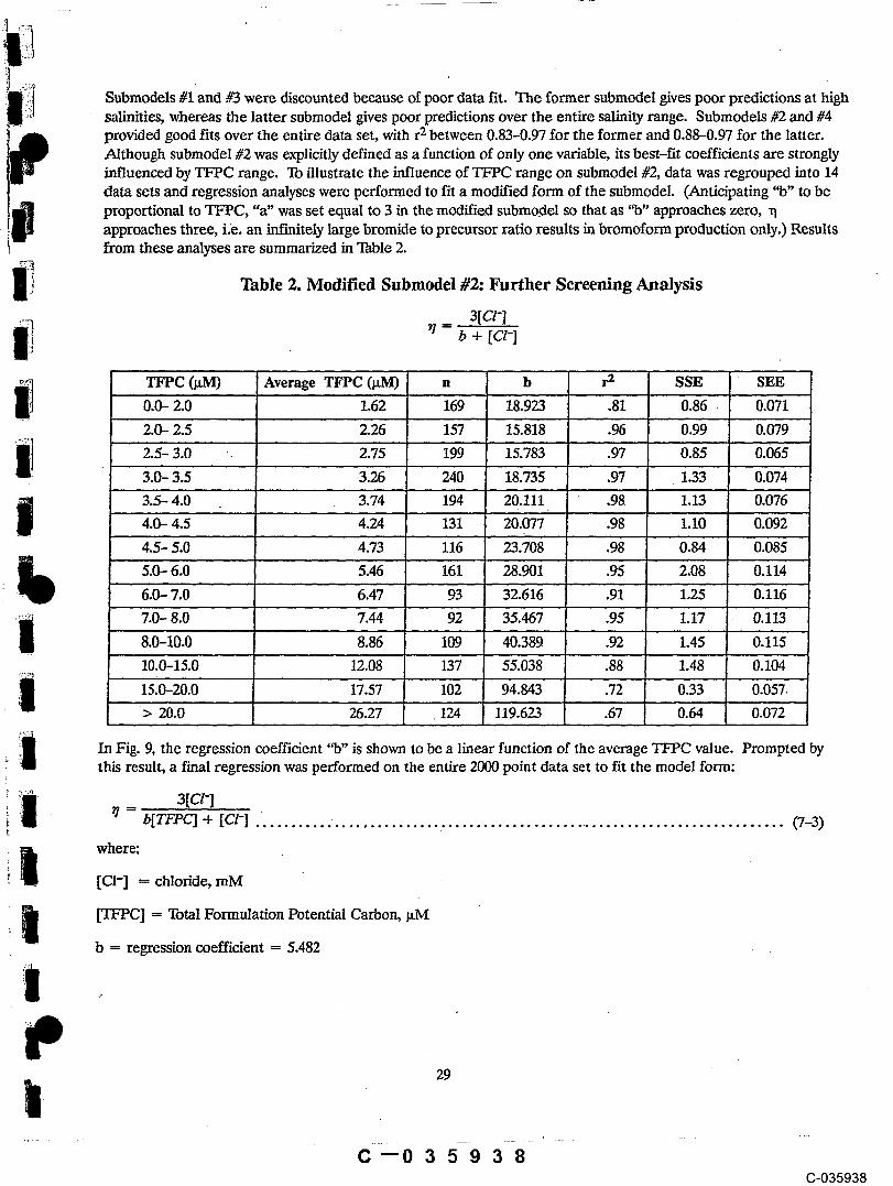
Submodels #1 and #3 were discounted because of poor data fit. The former submodel gives poor predictions at highsalinities, whereas the latter submodel gives poor predictions over the entire salinity range. Submodels #2 and #4provided good fits over the entire data set, with r2 between 0.83-0.97 for the former and 0.88-0.97 for the latter.Although submodel #2 was explicitly defined as a function of only one variable, its best-fit coefficients are stronglyinfluenced by TFPC range. To illustrate the influence of TFPC range on submodel #2, data was regrouped into 14data sets and regression analyses were performed to fit a modified form of the submodel. (Anticipating "b" to beproportional to TFPC, "a" was set equal to 3 in the modified submod, el so that as "b" approaches zero, -qapproaches three, i.e. an infinitely large bromide to precursor ratio results in bromoform production only.) Resultsfrom these analyses are summarized in Table 2.

Table 2. Modified Submodel Further Screening Analysis

3[ct-]i! ~ = b + [Ct-]

TFPC (pM) Average TFPC (~tM) n " b r~ ’ - SSE SEE0.0- 2.0 1.62 ’1~9 " 18.923 .81 0.86 - ~"’ 0.071

2.0- 2.5 2.26 157 "’ 15~’818 .96 0.99 ’ ’0.079

f 2.5- 3.0 ". 2.75 199 15.783 .97 0.85 0.065

3.0’- 3.5 3.26 240 I8.735 ’.97 i.33 0.0743.5- 4.0 3.74 194 20.111 " .98 1.13 13.0764.0- 4.5 4.24 131 " 20.0~7 .98 1.10 0.0924.5’" 5.0 4.73 116 23.708 .98 0.84 0.085

~ 5.0- 6.0 5.46 161 28.901 .95 2’.08 0.1146.0- 7.0 6.47 93 32.616 .91 1.25 0.116

~ 7.0-- 8.0 7.44 92 35.467 .95 1.17 0.113

| 8.0=10.0 8.86 109 40.389 .92 "i.45 1~.1"15

10.0-15.0 ’12.08 137 55.038 188 1.48 6.104’i5.0-2~.0" ’ 17.57 " 102 94.843 .72 0.33 0.057.> 20.0 "’ 26.27 124 119.69.23 .67 0.64 0.0~2

In Fig. 9, the regression coefficient "b" is shown to be a linear function of the average TFPC value. Prompted bythis result, a final regression was performed on the entire 2000 point data set to fit the model form:

3[ct-I~1 = b[TFPC] + [CI-] (7-3)

where:

[121-] --- chloride, mM

[TFPC] = Total Formulation Potential Carbon, ~tM

regression coefficient = 5.482

29

C--035938C-035938

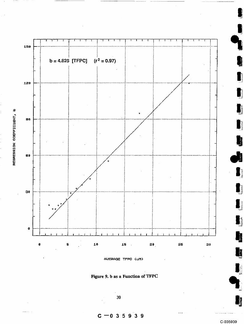
,.1,150

b = 4.825 [TFPC] (r2 = 0.97)

,/.20 .... ~ .................................. .~ ................................... ; ................................... ; ................................... : .................................. ; ........

AVERAGE TFPO

Figure 9. b as a Function of TFPC

C--035939 - -C-035939

An r2 value of 0.95, an SSE value of 19.86, and an SEE value of 0.099 were obtained for this relationship with thecoefficient "b" equal to 5.482. This relationship, Submodel #5, was selected as the best submodel form to predictBromine Incorporation Factor. Submodel #5 makes theoretical sense because it indicates the importance of thebromide to precursor ratio in influencing THMFP speciation. Eq. 7-3 can be rewritten in the form:

3[cl(7-4)

to further highlight the importance of this ratio. Fig. 10 shows the data from Fig. 7 as a function of the molarchloride to TFPC ratio and superimposes the relationship given in Eq. 7-4. Fig. 11 compares observed andpredicted values of ~q for submodel #5.

Spatial Variation

To analyze the spatial variation of "q, measured values were plotted for eight stations in the Delta. The first fourstations (see Fig. 12) represent export locations and include Banks Pumping Plant, Clifton Court Forebay,Delta-Mendota Canal, and Rock Slough. These stations are typically characterized by moderate concentrations ofchloride and TFPC. The next four stations (see Fig. 13) represent boundary stations and include a composite ofmany agricultural drains, Greene’s Landing, Mallard Island, and Vernalis. These stations represent diverseconditions and water qualities. Eq. 7-4 is superimposed on each data set in Figs. 12 and 13. Visually, model fit isgood at all stations. The most scatter exists at high CI:TFPC ratios for the composite agricultural drain data’set.

Bromine Distribution Factors

The Bromine Incorporation Factor quantifies an average distribution of THM compounds in a water sample. Topredict the concentrations of CHCI3,. CHC12Br, CHCIBr2, and CI--IBr3 that comprise this average value, a termcalled Bromine Distribution Factor is defined.

Bromine Distribution Factors, Or sN, define the proportion of TFPC that exists in each of the THMFP species for agiven water sample. N denotes the number of bromide atoms in the TI-IM species, a notation identical tO that usedby Gould et al.44 in their definition of Bromine Incorporation Factor:

[CHCI3]

so = CHCI3 Distn’bution Factor = [TFPC] ...................................................... (7-5)

[ CHCI2Br]

sl = CHC12Br Distribution Factor --- [TFPC] .................................................(7-6)

s2 =~ CHCIBr2 Distribution Factor --- [TFPC] .................................................(7-7)

[CHBr3]

s3 -~ CHBr3 Distribution Factor = [TFPC] .................................................. (778) .

C--035940C-035940

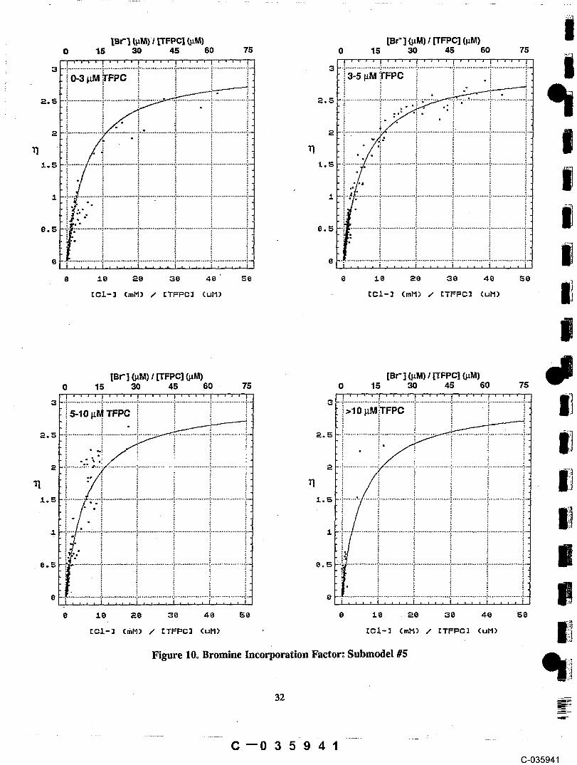
1 1

I:CL-:I (mH) / [TFPC] (uH) rcJ,-] (mH) / [TFPC] (uH)

Figure 10o Bromine Incorporation Factor: Submodel #5

32

C--035941C-035941

o

~-- PREDICTED

Fibre 11. Bromine Incorporation Factor: Obse~ed versus Predicted Values

33

C--O 3-5942G-035942

[Br- ] (~M) / [TFPC] (pM) [Br- ] (~M) / [TFPC] (~.M)

............... ~ ...............~ ................~ ...............~ ................:" ...............~’- ~ ¯ 5 -" ...............~ ................~ ................~ ...............~ ................: ................~’"

BANKS PUMPING PLAN~ ~ CLI~ON COURT~ FOREBAY

@.9

~.5 L 1.5 2 2.5 3 8 @.N 1 1.5 2 2.5 3

[CI-3 (mH) / [TFPC] (uH) [CI-3 (mH) / [TFPC] (uH)

1.s 3.0 4.s 0 1.s 3.o 4.5

8.5 1 ~.5 2 ~.5 3 @ 8.~ ¯ ~.5 2 2.5

[CI-3 (mM) / [TFPC] (uH) [Cl-] (mH) / [TFPC]

Figure 12o Bromine Incorporation Factor at Export Stations

34

C--035943C-035943

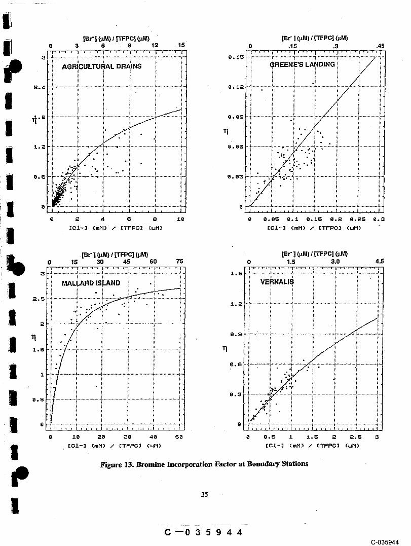
[Sr’] (I~M) I [TFPC] (}~M) [er" ] (FM) ! [TFPC] (I~M)3 S 9 12 r 15 0 .15 .3 .45

.................. + .................. ~ ................... ~ ...................................... ~’" ~ ---’"-""~---"~"-"’""~D~..~ ~ ~ . ~~

e. ~ -.~ ...............~ ................~. ...............~ .............. :~ ................~. .............AGRICULTURAL DRAINS . ~ ~REEN~’S LA

g . ~ "’~ ...............~ ................~" ...............~ ..............~ ..............."~ ................~’"

0.0B

0 I , , , , I , , , , I , , , , I , , , , I , , , ~ I ,..~ , ~ I

~ 4 ~ ~ ~0 0 0.05 0.~ 0.L5 0.~ 0.~5 0.3

ICI-] (mN) / [TFPC~ (uM) [C~-] (mM) / [TFPC] (uM)

[Br’] (~M) / FFPC] (~M) [Br" ] (~M) / FFPC] (~M)15 30

45~

60 75 0 1.5 3.0 4.5

~+ ~ L. 5 ~ ..................~ ...............~ ................ . :

. : VERNALISMAL~RD IS~ND ~

." 1.~ ...................................................................................................~’"

0.9 " ........... ~ ...........~ ....

~"I ~ ~ ~ , I , ,’, , I , , , , I , + , , , , ~ , , ,,~ ~ I

10 20 30 40 58 0 e+5 1 ~.5 ~ 2.5 3

[C1-3 (mH) / [TFPC] (QM) [CZ-] (mM) / [TFPC3 (uM)

Fibre 13. Bromi.e I.cor~ratio. Factor at Bou.da~ ~tatio.s

C--035944C-035944

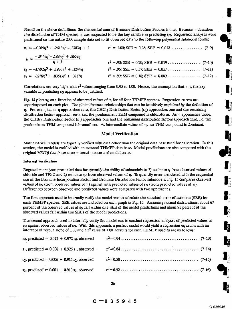
Based on the above definitions, the theoretical sum of Bromine Distribution Factors is one. Because ~q describesthe distribution of THM species, rl was suspected to be the key variable in predicting SN. Regression analyses wereperformed on the entire 2000 sample data set to fit observed data to the following polynomial submodel forms:

so -- --.0285~i3 + .2613~q2 -.8703~ + i r2 = 1.00; SSE --- 0.28; SEE = 0.012 .................(7-9)

-.0446r/~- .1888~ + .8659r/~/+ 1 r2 =.95; SSE -- 0.70; SEE = 0.019...~ ...............(7-10)

s2 --- --.0792rl3 + .1936~q2 + .1244~1 r2 =.96; SSE = 0.57; SEE = 0.017 ..................(7-11)

s3 --- -0250~13 + .0351~12 + .0017rl r2 =.99; SSE = 0.18; SEE = 0.009 ..................(7-12)

Correlations are very high, with r2 values ranging from 0.95 to 1.00. Hence, the assumption~that ~ is the keyvariable in predicting SN appears to be justified.

Fig. 14 plots SN as a function of observed values of ~1 for all four THMFP species. Regression curves aresuperimposed on each plot. The plots illustrate relationships that can be intuitively explained by the definition of"q. For example, as "q approaches zero, the CHC13 Distribution Factor (so) approaches one and the remainingdistn’bution factors approach zero, i.e., the predominant THM compound is chloroform. As "q approaches three,the CI-IBr3 Distn’bution Factor (s3) approaches one and the remaining distribution factors approach zero, i.e. thepredominant TH2VI compound is bromoform. At intermediate values of al, no THM compound is dominant

Model Verification

Mathematical models are typically verified with data. other than the original data base used for calibration. In thissection, the model is verified with an external THMFP data base. Model predictions are also compared with theoriginal MWQI data base as an internal measure of model error.

Internal Verification

Regression analyses presented thus far quantify the ability of submodels to 1) estimate ~1 from observed values ofchloride and TFPC and 2) estimate SN from observed values of a~. To quantify error associated with the sequentialuse of the Bromine Incorporation Factor and Bromine Distribution Factor submodels, Fig. 15 compares observedvalues of sN (from observed values of ~q) against with predicted values of SN (from predicted values of ~1).Differences between observed and predicted ,,~ues were compared vdth two approaches.

The first approach used to internally verify the model was tO calculate the standard error of estimate (SEE) foreach THMFP species. SEE values are included on each graph in Fig. 15. Assuming normal distributions, about 67percent of the observed values of sN fall within one SEE of the model predictions and about 95 percentof theobserved values fall within two SEEs of the model predictions.

The second approach used to internally verify the model was to conduct regression analyses of predicted values ofs~ against observed values of SN. With this approach, a perfect model would yield a regression equation with anintercept of ze.ro, a slope of 1.00 and a r2 value of 1.00. Results for each THMFP species are as follows:

sO, .predicted = 0.027 + 0.972 so, observed r2 = 0.94 ..........................................(7-13)

sl, predicted = 0.006 + 0.926 sl, observed r2---0.84 .......................................... (7-14)

s2, predicted = 0.006 + 0.915 s2, observed r2=0.88 ..........................................(7-15)

s3, predicted = 0.001 + 0.910 s3~ observed , r2 = 0.92 ..........................................(7-16)

36

C--035945C-035945

.., .............. =. ............... .’,. ...............;. ............... ;. ............... :. .................:.,

"’ iSTRi UTIO ;FA,CTbR } DiSrR’BUTiON FACTO ~ r2 = 0.953

8 o 6 @ ° 6 " ..............."." ................:" ...............~ ...............~ ...............": ................

"i} 8,4 ’i ............... ~ ......... "~’~. ............... ~ ............... ~ ............... ~ ............... ~" ¯. 4 ’’= ............... ~’~’""’: ............ ~ ...........................................................

~..

i 8 I ,, , , I , ,.,_, I , , , , I .... I , , , , I .... 1

8 8.5 I 1.5 2 2.5 3

CHCIBr2 DISTRIBUTION FACTOR CHBr3 DISTRIBUTION FACTOR

~.8 ....................................................................................................... 8.8

~ :8.6 "’ .......... ~ .........:" .......................... ~ ...............: ............... 8.6 ............................. ~ .........

~.~ ~.2 ’" - ’~ ""~’,’"’~ ...............~ ...............~"

L.~ ~ .~~ ....... ............... ............

Fibre 14. Bromine Distribution Factors

37

C--035946C-035946

Figure 15o Bromine Distribution Factors: Observed versus Predicted Values

38

�’035947C-035947

Intercepts, slopes and correlations indicate that the model generally provides good predictions; the best preditionsbeing for so.

External Verification

Model verification was also conducted with an external data base. The external data base was developed by Amy etal.29 The data set received from the authors included 1,025 samples with chlorine residuals greater than zero. Thedata set reported in the literature included 995 ~mples. This slightly larger data set was utilized to verify theBromine Incorporation Factor and Bromine Distribution Factor submodels.

To verify the Bromine Incorporation Factor submodei, the external data base was segregated to isolate data pointsthat more closely reflect DWR’s THMFP test conditions. A total of 64 data points were selected so that reactiontime was equal to seven days and reaction temperature was equal to 20°C. While other parameters such as pH,bromide and TOC are within the ranges observed in the Delta, the range of chlorine dose (1.5-69 rag/L) utilized inthe external data base is much lower than DWR’s test dose of 120 mg/L. Fig. 16 plots the 64 data points along withthe curve given in Eq. 7-4 as a function of the molar ratio of bromide to TFPC. The chloride to TFPC ratio in Eq.7-4 was multiplied by 1.5 to "convert" it to an equivalent bromide to TFPC molar ratio, assuming an open oceanwater correlation between bromide and chloride (see Eq. 4-4). Fig. 16 shows a good visual comparison between theexternal data base and the Bromine Incorporation Factor submodel given in Eq. 7-4. A SEE value of 0.132compares favorably with the SEE value of 0.099 computed for the MWQI data calibration of Eq. 7-4. A regressionanalysis of predicted values against observed values was conducted. Again, a perfect model would yield aregression equation with an intercept of zero, a slope of 1.00 and a r2 value of 1.00. The analysis resulted in anintercept of 0.079, a slope of 0.865, and a r2 value of 0.92. Although the correlation is pretty good, the interceptand slope indicates that the model tends to overpredict at low values of ri and underpredict at high values of ~.The difference in chlorine dose between the external data base and the MWQI data base is a likely explanation forthe model underpredicti0n at’ high values of n. Variability in temperature (T= 25°C under DWR test conditions)and variability in pI-I may also explain some of the deviation between model predictions and observed values.

To verify the Bromine Distribution Factor submodels, the entire data base was utilized to compare predicted andobserved values. Fig. 17 plots the 1025 data points along with the curves given in Eqs. 7-9 through 7-12 asfunctions of observed Bromine Incorporation Factor. The external data base visually follows the submodelrelationships as well or better than the MWQI data base (compare with Fig. 14). Similarities between SEE valuesfor the external data base (see Fig. 17) and for the MWQI data base (see Eqs. 7-9 through 7-12) confirm this visualobservation. Regression analyses of predicted ~lues against observed values were conducted, resulting in thefollowing:

so, predicted = -0.012 + 1.024 so, observed r2-1.00 .......................................... (7-17)

sl, predicted --- -0.004 + 0.958 sl, observed r2=0.96 (7-18)

s2, predicted = -0.008 + 0.964 s2, observed r2=’0.99 (7719)

s3, predicted = .0.002 + 0.930 s3, observed r2=0.99 ..........................................(7-20)

Intercepts, slopes and correlations indicate that the model provides excellent predictions of Bromine DistributionFactors. This comparison shows that THMFP species form in a predictable fashion under varying test conditions.Because Eqs. 7-17 through 7-20 were developed with observed (and not predicted) values of ~, the intercepts,slopes and correlations from these equations should not be directly compared with those given in Eqs. 7-13 through

C--035948C-035948

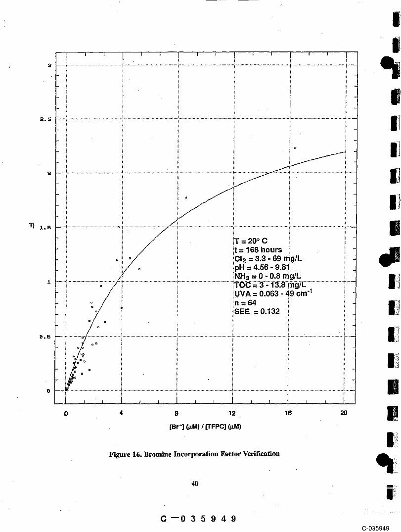
Figure 16. Bromine Incorporation Factor Verification

4O

C--035949C-035949

SEE = .0.015 SEE = 0.(Y23

Figure 17. Bromine Distribution Factors Verification

41

C--035950C-035950

Example Problem

To partially illustrate the model framework established in this report, an example problem is presented in Fig. 18and is discussed further below. The problem specifically shows how the precursor simulation model (DWRDSM)and the THMFP empirical relationships (Bromine Incorporation Factor and Bromine Distribution Factors) fitwithin the overall model framework. DWRDSM was run in a steady state.mode to simulate transport of TFPC andtotal dissolved solids (TDS) in the Delta during the month of July 1988 (see Chapter 8). Historic water qualityobservations were input as boundary conditions. SimuIation model resuIts at Clifton Court Forebay were utilized asinput to .the following steps: ~

1, Simulation model results are converted to units consistent with Eq. 7-3. If TDS or EC is used to simulatesalinity transport (as was the case in the example), an appropriate conversion must be made to determine chlorideconcentration.

2. After water quality parameters are converted to appropriate concentration units, the Bromine IncorporationFactor is determined from Eq. 7-3 with b = 5.482.

3. Bromine Distn’bution Factors are calculated as a function of the Bromine Incorporation Factor determined inStep 2. If a calculation results in a negative number, that distribution factor is assumed to be zero. An so value of0.46 means that 46 percent of the TFPC is in the form of CHCI3. An Sl value of 0.31 means 31 percent of theT!PC is in the form of cHCi2Br. After all four distribution factors are calculated, the values are summed.Theoretically, the sum should equal one. If the sum does not equal one as in the example, a correction is made inStep 5.

4. THMFP molar concentrations are calculated as the product of Bromine Distribution Factors and TFPCo

5. THMFP mass concentrations are calculated as the product of molar concentration and molecular weight. ~Because the distribution factor sum is not equal to one in the example, the mass concentrations is divided by theBromine Distnqgution Factor sum.

PROBLEM STATEMENT: A transport model simulation of THM precursors in the Delta during July 1988was conducted (details are provided in Chapter 8). Results indicated the following precursor concentrationsat Clifton Court Forebay gates:

TFPC = 3O i~g/LTDS = 473 mg/L

Estimate THMFP species and total THMFP mass concentrations at Clifton Court Forebay.

STEP 1: Calculate TFPC and Chloride STEP 2: Calculate Bromine Incorporation Factor (-q)Molar Concentrations

3 [C~’]30 ~g/L = 2.50 I~M ~1 - 5.482 x [-I-FiSC] + [Ci-][TFPC] = 12 I~g/t~mole (3

(3)(4.99)per salinity relationship [47]: TI = (5.482)(2.50) + 4.99Cl’= "47.95 + 0.4751 x TDS = 177 mg/L

[Cl’] = 177 mg/L = 4.99 mM ’q = 0.8035.45 mg/mmoi’e

STEP 4: Calculate Preliminary THMFPSTEP 3: Calculate Bromine Distribution Molar Concentrations

Factors (SN) [CHCI3] = So x [TFPC] = 0.46 × 2.50 p.M = 1.15 I~M

So = -.0285~3 + .2613~2 - .8703-q+ 1 [CHCI2Br] = $1 x [TFPC] = 0.31 x 2.50 ~M = 0.775

So = -.0285 (.80)3 + .2613 (.80)2 - .8703 (.80) + 1 [CHCIBr2] = $2 x [TFPC] = 0.18 x 2.50 I~M = 0.45

So= O.46[CHBr3] = $3 x [TFPC] = 0.04 x 2.50 I~M = 0.10

$1 = (-.0446~13- .1888TI2 + .8659~1) / (’q +1)

S1 = (-.0446 (.80)3- .1888 (.80)2 + .8659 (.80)) /(.80 + 1)

$1 = 0.31STEP 5: Calculate Revised THMFP

Mass Concentrations$2 = -.0792rl3 + .1936TI2 + .1244TI Adjust preliminary values such that ~sN = 1.00S 2 = -.0792 (.80)3 + .1936 (.80) 2 +. 1244 (.80)

$2= 0.18 CHCI3 = 1.15 ~M x 119.36 i~g/~mole= 139 p.g/L0.99

CHCI 2Br = 0.775 ~M x 163.82 I~g/l~mole = 128 i~g/L0.99

$3= .0250~13 + .0351.TI2 +.0017~1S3 = .0250 (.80)3 + .0351 (.80)2 +.0017 (.80)

0.45~MCHClBr2 0.99 x 208.28 ~g/~mole = 95 p.g/L

$3= 0.04CHBr3 = 0.10 F.M x 252.74 p.g/~mole = 26 p.g/L

0.99

~SN= 0.46 + 0.31 + 0.18 + 0.04 = 0.99 Total THMFP = 139 + 128 + 95 + 26 = 388 ~g/L

Figure 18. THMFP Model Methodology: Example Problem

43

C--035952C-035952


C--035953C-035953

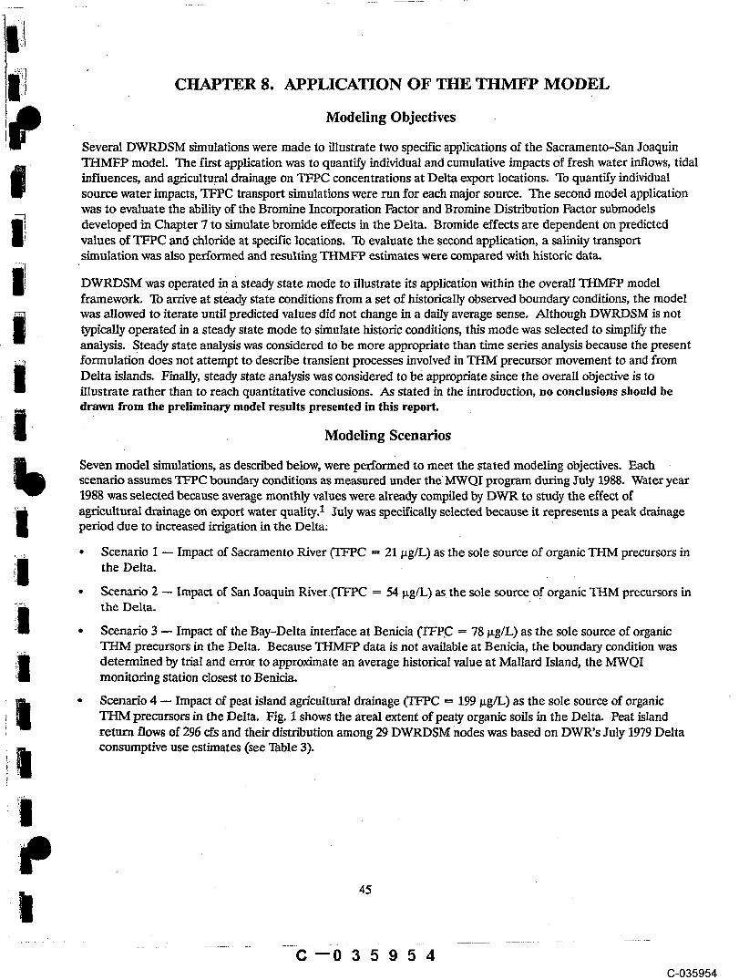
Several DWRDSM simulations were made to illustrate two specific applications of the Sacramento-San JoaquinTHMFP model. The first application was to qnanti£y individual and cumulative impacts or fresh water in.flows, tidalinfluences, and agricultural drainage on TFPC concentrations at Delta export locations. To quantify individualsource water impacts, TFPC transport simulations were run for each major source. The second model applicationwas to evaluate the ability of the Bromine Incorporation Factor and Bromine Distn’bution Factor submodelsdeveloped in Chapter 7 to simulate bromide effects in the Delta. Bromide effects are dependent on predictedvalues of TFPC and chloride at specific locations. To evaluate the second application, a salinity transportsimulation was also performed and resulting TITMFP estimates were compared with historic data.

DWRDSM was operated in a steady state mode to illustrate its application within the overall THMFP modelframework. To arrive at steady state conditions from a set of historically observed boundary conditions, the modelwas allowed to iterate until predicted values did not change in a daily average sense. Although DWRDSM is nottypically operated in a steady state mode to simulate historic conditions, this mode was selected to simplify theanalysis. Steady state analysis was considered to be more appropriate than time series analysis because the presentformulation does not attempt to describe transient processes involved in THM precursor movement to and fromDelta islands. Finally, steady state analysis was considered to be appropriate since the overall objective is toillustrate rather than to reach quantitative conclusions. As stated in the introduction, no conclusions should bedrawn from the preliminary model results presented in this report.

Modeling Scenarios

Seven model simulations, as described below, were performed to meet the stated modeling objectives. Eachscenario assumes TFPC boundary conditions as measured under theMWQI program during July 1988. Water year1988 was selected because average monthly values were already compiled by DWR to study the effect ofagricultural drainage on export water quality.1 July was specifically selected because it represents a peak drainageperiod due to increased irrigation in the Delta:

* Scenario 1 -- Impact of Sacramento River (TFPC = 21 ~tg/L) as the sole source of organic THM precursors inthe Delta.

¯ Scenario 2 -- Impact of san Joaquin RiverOqzPC = 54 ~tgFL) as the sole source of organic THM precursors inthe Delta.

o Scenario 3 -- Impact of the Bay-Delta interface at Benicia (TFP,C = 78 ~tg/L) as the sole source of organicTHM precursors in the Delta. Because THMFP data is not available at Benicia, the boundary condition wasdetermined by trial and error to approximate an average historical value at Mallard Island, the MWQImonitoring station closest to Benicia.

o Scenario 4 -- Impact of peat island agricultural drainage (TFPC = 199/tg/L) as the sole source of organicTHM precursors in the Delta. Fig. I shows the areal extent of peaty organic soils in the Delta..Peat islandreturn flows of 296 cfs and their distribution among 29 DWRDSM nodes was based on DWR’s July 1979 Deltaconsumptive use estimates (see Table 3).

C=035954C-035954

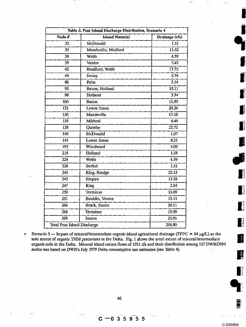
Table 3. Peat Island Discharge Distribution, Scenario 4

Node # .... Island Name(si ’ Drainage (cfs)’

32 McDonald 1.31’ 35 Mandeville, Medford 11.52

’ 38" Webb ’"39 Venice 7.43

42 Bradford, Webb 17.7544 Jersey 5.74

86 Palm 3.1493’ Bacon, Holl~nd ........ 1~.1198 Holland . 3.34

100 Bacon 11.9~121 Lower Jones 20.26130 a de, le 17.10135 Mildred ’ 4.4b

138 O~nby 22.72140 McDonald 1.0714i Lower Jones i2i ’ "195 Woodward "’ 4.09

- 21g Holland 1.5822~ Webb _ 4.59

226 Bethel 1.5124~ King, Rindge .... 22.13245 Empire 13.38

’" 247 I~g "’ ’ 2.84250 Terminus 15.09

251 Bouldin, Venice 13.51266 Brack, Staten 20.11268 Terminus 15.09269 Staten 25.91

T̄otal Peal Island Discharge 296.00

¯ Scenario 5 -- Impact of mineral/intermediate organic island agricultural drainage O’FPC = 84 gg/L) as thesole source of organic THM precursors in the Delta. Fig. 1 shows the areal extent of mineral/intermediateorganic soils in the Delta. Mineral island return flowsof 1311 cfs and their distribution among 157DWRDSMnodes was based on DWR’s July 1979 Delta consumptive use estimates (see Table 4). . ~

C--035955G-035955

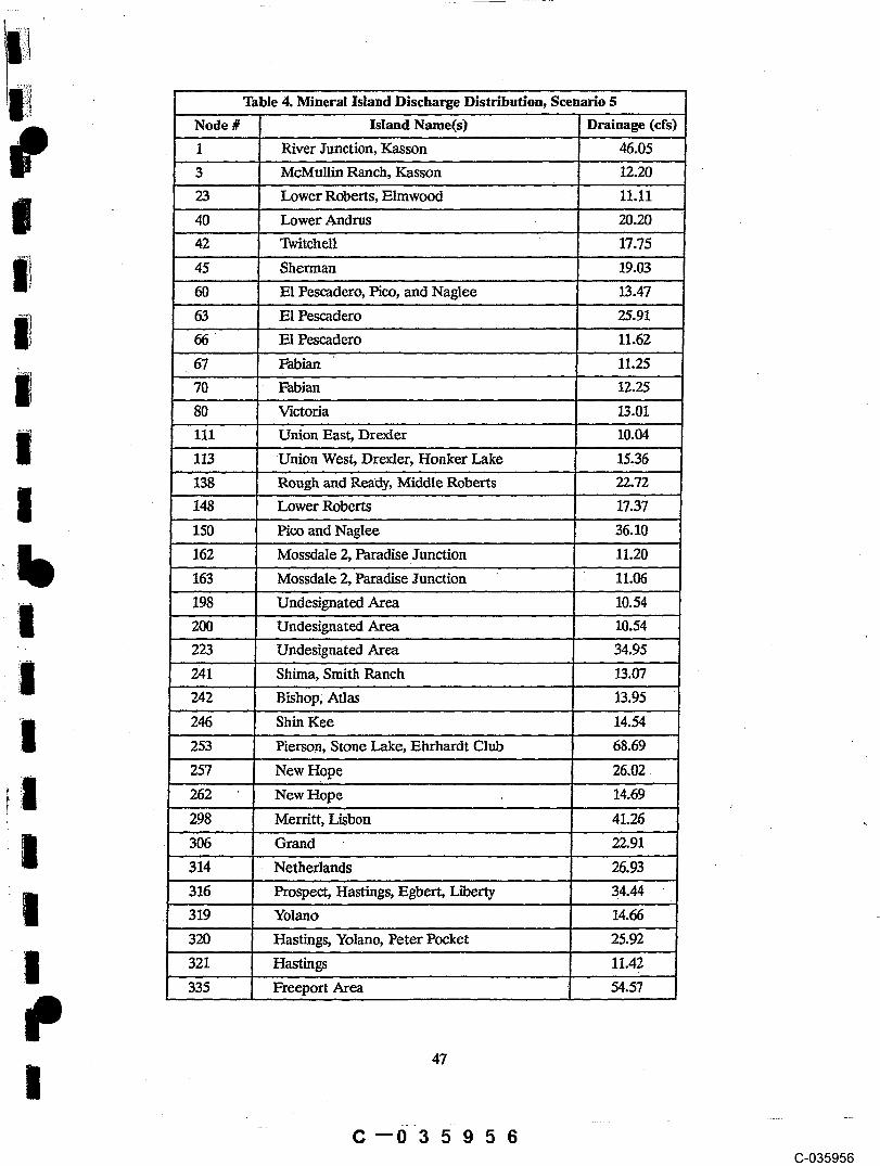
Table 4. Mineral Island Discharge Distribution, Scenario $Node #

, Is.land Nam.e(s)Drainage (cfs)

1 River Junction, Kasson 46.05

3’ McMullin Ranch, Kasson J2.2023 Lower Roberts, Elm~vo0d i1.1140 LoUver Andrus 20.2042 Twitchell 17.75

45 Sherman 19.03

60 E1 Pescadero, Picol and Naglee .........13.47

63 E1 Pescadero 25.91

66 " El Pes~.adero .... 11.62

67 Fabian 1i.25Fabian 12.2570

80 Victoria 13.01ill Union East, Drexler 10.04

113 r~ni0n ’;West, Drexler, ~onker"Lake 15~36"~38 R~ugtt and Ready, Middle Roberts 22.72

148 L~wer Roberts ..... 17.37150 Pi’co and Naglee 36.10

162 Mossdale 2, Paradise Junction 11.20

163 Mossdale 2, Paradise Junction 11.06

198 Undesignated Area 10.54

200 Undesignated Area 10.54

223 Und~"si~aated Area ~4.~5

24i Shima, Smith Ranch 13.07242 Bishop; Atlas 13.95

246 Ke ’ 14.54253 Pierson, Stone Lake,’Ehrhardt Club 68.69

257 Ne~ Hope " 26.02.262 New Ho~e 14.69

298 Merritt, Lisbon 41.i6

306 Grand 2Z91

314 Netherlands ’" 26.93

316 Prospect, Hastings, Egbert, Liberty 34.44-319 Yolano 14.66320 Hastings, ¥olano, Peter Pocket 25.92321 Hast~gs 11.42

335 Frelport ~kr~a " ~4.57 ,",

C--035956C-035956

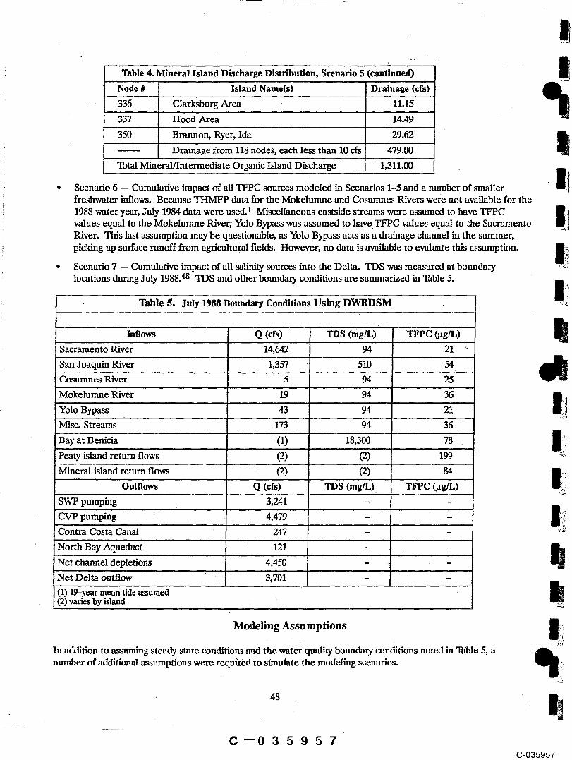
Table 4. Mineral Island Discharge Distribution, Scenario $ (continued)

Node # Island Name(s) Drainage (cfs)

336 Clarksburg Area 11.15

337 Hood Area 14.49

350 Brannon, Ryer, Ida 29.62DraYage from 118 nodes, each less than 10 cfs 479.00

To~al Mineral/Intermediate O~ganic Island Discharge 1,311.’00

¯ Scenario 6 -- Cumulative impact of all TFPC sources modeled in Scenarios 1-5 and a number of smallerfreshwater inflows. Because THMFP data for the Mokelumne and Cosumnes Rivers were not available for the!988 water year, July 1984 data were used.1 Miscellaneous eastside streams were assumed to have TFPCvalues equal to the Mokelumne River; Yolo Bypass was assumed to have TFPC values equal to the SacramentoRiver. This last assumption may be questionable, as Yolo Bypass acts as a drainage channel in the summer,picking up surface runoff from agricultural fields. However, no data is available to evaluate this assumption.

¯ Scenario 7 -- Cumulative impact of all salinity sources into the Delta. TDS was measured, at boundarylocations during July 1988.48 TDS and other boundary conditions are summarized in Table 5.

Table $. July 1988 Boundary Conditions Using DWRDSM¯Inflows Q (cfs) TDS (mg/L) TFPC (~Lg/L)

Sacramento River 14,642 94 21

San Joaquin River 1,357 510 54

Cosumnes River 5 94 25

Mokelumne Rive~: .... 19 94 36

Yolo Bypass 43 94 21

Misc, Streams .... 17~ .... 94 36

Bay at Benicia .(1) 18,300 78~eaty island return flows (2) (2) 199

Mineral island return flows (2) (2) 84

Outflows "-Q (cfs) TDS (rag/L). TFPC (~g/L)SW’~ pumping 3,241’ - -CVP pumping 4,479 - -Contra Costa Canal "" 247 - -North Bay Aqueduct ...... 121 - -i~let’channel depletions’" 4,450 - - ""

Net Delta outflow~

3,701 - -(’1) 19-year mean tide assumed(2) varies by island

Modeling Assumptions

In addition to assuming steady state conditions and the water quality boundary conditions noted in Table 5, anumber of additional assumptions were required to simulate the modeling scenarios.

48

C--035957(3-035957

¯ July 1988 hydrology was assumed to follow historic inflow, outflow and pumping values compiled in DWR’sDAYFLOW data base.49 Net flow directions, which represent average tidal conditions during July 1988, aredepicted in Fig. 19.

o’ The difference between agricultural channel diversions and returns was assumed to emulate the consumptiveuse pattern of July 1979, a similar hydrologic period.

¯ A 19-year mean tidal cycle was assumed as the tidal forcing function in the Delta,

¯ Salinity from agricultural drainage was assumed to emulate the pattern observed in the Delta during 1954 and1955"6

¯ TFPC was assumed to act as a conservative constituent in the Delta and to represent precursor effects. Bothof these assumptions are discussed at length in Chapters 3 and 5.

¯ TDS was assumed to act as a conservative constituent in the Delta and represent bromide in the Delta. Saltsare generally considered to act conservatively in natural waters. Correlations between TDS and chloride havebeen well established in the Delta.47 And for water exported from the Delta through the SWP, the ionic ratiobetween chloride and bromide appears to be similar to that of open ocean water.2!,22

Results

Results from the seven model scenarios are summarized herein. To emphasize the individual impact on exportwater quality from each precursor source, TFPC at Clifton Court Forebay inlet gates is reported for each scenario.

Scenario 1

Fig. 20 shows the influence of the Sacramento River on TFPC transport is substantial throughout most of theDelta. Since most Delta inflow comes from.the Sacramento River, this result is not too surprising. Scenario 1estimates the Sacramento River contributes 19 t~g/L TFPC at Clifton Court Forebay under steady state conditions.DWRDSM reached steady state in approximately 70 days of simulation.

Scenario 2

Fig. 21 shows the influence of the San Joaquin River on TFPC transport is limited to the southern part of theDelta. This result can be explained by the net flow directions shown in Fig. 19. The model run predicts that SanJoaquin River water flows entirely toward the Central Valley Project (CVP) Delta-Mendota Canal intake. Anidentical flow pattern was observed in the field1 by tracing selenium under similar low flow conditions. Scenario 2indicates that the San loaquin River does not contn"oute TFPC at Clifton Court Forebay under steady state lowflow conditions. DWRDSM reached steady state in approximately 12 days of simulation.

Scenario 3

Fig. 22 shows the influence of the Bay-Delta interface on TFPC transport is limited to the western Delta. Aboundary condition at Benicia was not available from existing TFPC data to directly perform this model run.Therefore, a trial and error method was employed to determine an appropriate valu.e.

Through trial and error, it was determined that a TFPC boundary condition of 78 Ixg/L at Benicia produced resultscomparable with observed values at Mallard Island. Mallard Island, for which a 52 pLg/L TFPC concentration wasmeasured, is the Delta monitoring location most representative of Suisun Marsh and San Francisco Bay influences.

C--035958(3-035958

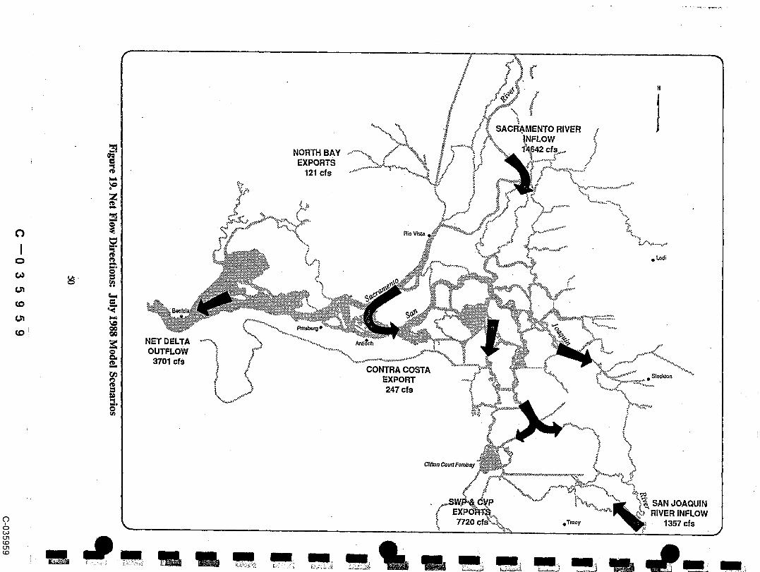
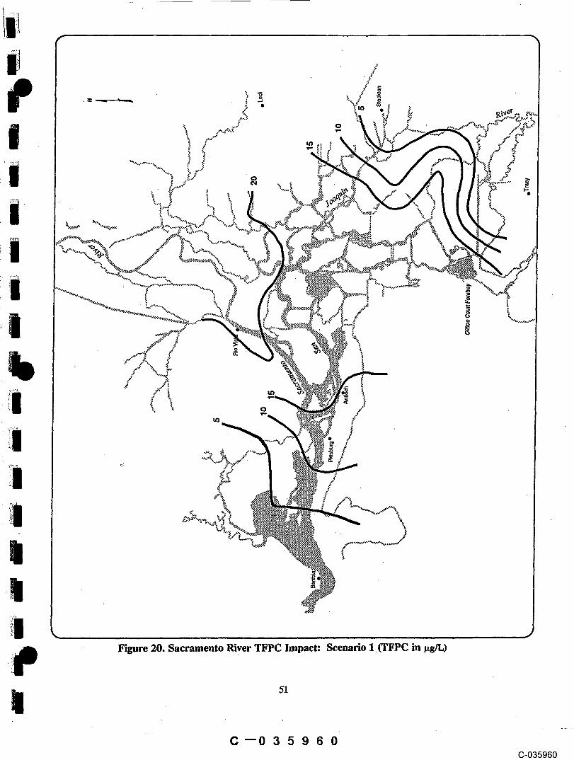
Figure 20. Sacramento River TFPC Impact: Scenario 1 .(TFP� in pg/L)

C--035960G-035960

1,969~0-0

I, 9 6 ~ ~; 0--0

Figure 22. Bay TFPC Impact: Scenario 3 (TFPC in/~g/L)

C--035962(3-035962

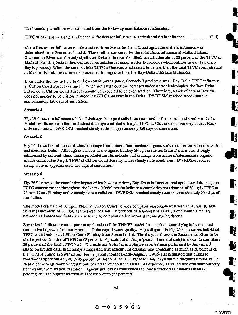
The boundary condition was estimated from the following mass balance relationship:

TFPC at Mallard ffi Benicia influence + freshwater influence + agricultural drain influence ............(8-1)

where freshwater influence was determined from Scenarios 1 and 2, and agricultural drain influence wasdetermined from Scenarios 4 and 5. These influences comprise the total Delta influence at Mallard Island.Sacramento River was the only significant Delta influence identified, contn~buting about 20 percent of the TFPC atMallard island. (Delta influences are more substantial under wetter hydrologies when outflow to San FranciscoBay is greater.) When the sum of Delta TFPC influences is estimated to be less than the total TFPC concentrationat Mallard Island, the difference is assumed to originate from the Bay-Delta interface at Benicia.

Even under the low net Delta outflow conditions assumed, Scenario 3 predicts a ~mall Bay-Delta TFPC influenceat Clifton Court Forebay (2 ~tg/L). When net Delta outflow increases under wetter hydrologies, the Bay-Deltainfluence at Clifton Court Forebay should be expected to be even smaller. Therefore, a lack of data at Beniciadoes not appear to be critical in modeling TFFC transport in the Delta. DWRDSM reached steady state inapproximately 120 days of simulation.

Scenario 4

Fig. 23 shows the influence of island drainage from peat soils is concentrated in the central and southern Delta.Model results indicate that peat island drainage contributes 6 ~tg/L TFPC at Clifton Court Forebay under steadystate conditions. DWRDSM reached steady state in approximately 120 days of simulation.

Scenario S

Fig. 24 shows the influence of island drainage from mineral/intermediate organic soils is concentrated in the centraland southern Delta. Although not shown in the figure, Lindsey Slough in the northern Delta is also stronglyinfluenced by mineral island drainage. Model results indicate that drainage from mineral/intermediate organicislands contn"outes 3 ttg/L TFPC at Clifton Court Forebay under steady state conditions. DWRDSM reachedsteady state in approximately 120 days of simulation.

Scenario 6

Fig. 25 illustrates the cumulative impact of fresh water inflows, Bay-Delta influences, and agricultural drainage onTFPC concentrations throughout the Delta. Model results indicate a cumulative contribution of 30/sg/L TFPC atClifton Court Forebay under steady state conditions. DWRDSM reached steady state in approximately 200 days ofsimulation.

The model estimate of 30 ~tg/L TFPC at Clifton Court Forebay compares reasonably well with an August 9, 1988field measurement of 38 ~tg/L at the same location. In previous data analysis of TFPC, a one month time lagbetween estimates and field data was found to compensate for inconsistent measuring dates.1

Scenarios 1-6 illustrate an important application of.the THMFP model formulation: quantifying individual andcumulative impacts of source waters on Delta export water quality. A pie diagram in Fig. 26 summarizes individualTFPC contn"outions at Clifton Court Forebay from Scenarios 1-6. The diagram shows the Sacramento River to bethe largest contributor of TFPC at 63 percent. Agricultural drainage (peat and mineral soils) is shown to contrx"oute30 percent of the total TFPC load. This estimate is similar to a simple mass balance performed by Amy et al.5Based on limited data, their analysis suggested that agricultural drainage may contribute as much as 20 percent ofthe THMFP found in SWP water. For irrigation months (April-August), DWR1 has estimated that drainagecontn~autes approximately 40 to 45 percent of the total Delta TFPC load. Fig. 27 shows pie diagrams similar to Fig.26 at eight MWQI monitoring stations located throughout the Delta. As expected, TFPC source contributions varysignificantly from station to station. Agricultural drains contn’outes the lowest fraction at Mallard Islar~d (2percent) and the highest fraction at Lindsey Slough (53 percent).

C--035963G-035963

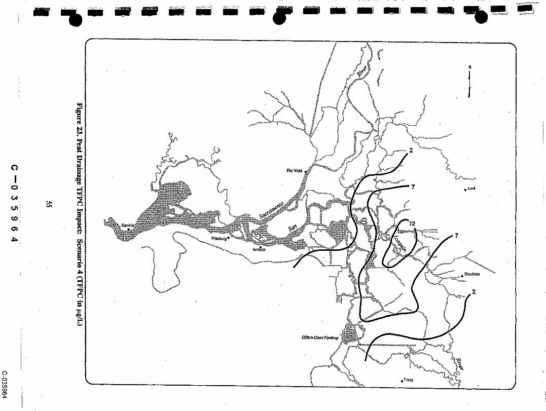
i

Bay Inflow2 (7%)

MineralIsland Drainage

3 (10%)

Peat SacramentoIsland River &

Drainage Miscellaneous6 (20%) Fresh Inflow

19 (63%)

Figure 26. TFPC at Clifton Court Forebay: Scenario 6 (in ~glL)

58

C--035967C-035967

¯ Sacramento

SAC RIVER & MISC FRESH INFLOWSAN JOAQUIN RIVERPEAT ISLAND DRAINAGE

i-~i MINERAL ISLAND DRAINAGEiY’2722R BAY INFLOW

RioLINDSEY

32 ~g/L

RIOVISTA LCONNECT,22 ~g!L 33 p,g/L

ROCKSL

MALLARDIS 29 I~g/L47 ~g/L

MIDDLER32 I~J/L

CLIFTONDMC , 30 I~g/L

34 ~g/L

Figure 27. TFPC at Selected MWQI Monitoring Stations: Scenario 6

C--035968C-035968

Scenario 7

To illustrate another important THMFP model application (simulating bromide effects from the BromineIncorporation Factor and Bromine Distribution Factors submodels), Delta-wide salinity transport was simulated inScenario 7. Fig. 28 shows steady state salinity values as measured by TDS. A TDS concentration of 473 mg/L,which translates into a chloride concentration of approximately 180 rag/L, is predicted at Clifton Court Forebay..TDS salinities represent proportional chloride (and thus bromide) concentrations throughout the Delta.

Comparison with I-Iistorie Data

DWRDSM steady state results for TFPC and TDS at the eight MWQI monitoring stations located in Fig. 27 wereused to predict chloride, Bromine Incorporation Factor 01) and THMFP values (CHCI3, CHC/2Br, CHC1Br2,CHBr3) at each location. These values, in addition to TFPC, are compared with historic data in Fig. 29. THMFPestimates compare very well with historic data at Clifton Court Forebay, Delta-Mendota Canal, Rock Slough andMallard Island. Although historic data were not available at Rio Vista, m0del values were reported to show thatthe model correctly reflects low THMFP concentrations at fresh water stations. The close agreement betweenpredicted and observed values at these stations makes the model formulation appear quite promising.

Deviations between predicted and observed values of THMFP are greatest at stations LcONNECT, LINDSEY,and MIDDLER. All three stations are shown in Fig. 27. THMFP at these stations appears to be heavilyinfluenced by agricultural drainage, highlighting the need to develop relationships that more accurately describeagricultural drainage quality in the Delta.

Although predicted and observed TFPC values are similar at LCONNECT, the chloride estimate of 76 mg/L issubstantially greater than the observed value of 10 mg/L. This devid~ion results in much higher BromineIncorporation Factor (0.37 in~tead of 0.17) and thus higher bromomethane concentrations. Because of a goodTFPC prediction, the chloroform estimate is similar to the observed value.

The high deviation in chloride values at LCONNECT is partially attn"outed to DWRDSM and partially to anapparent anomaly in the TDS:C1- conversion. DWRDSM overpredicted TDS by a factor of two, predicting a valueof 232 mg/L while a nearby station (Little Potato Slough) was observed at 103 mg/L.4s TDS was not measured atLCONNECT during July 1988. However, by converting the predicted value of TDS to chloride ~with a relationshipdeveloped for another nearby station (South Fork Mokelumne River below Sycamore Slough)~47 the overpredictionwas magnified to a factor of eight. ..:

LINDSEY suffers from the opposite problem descn~oed at LCONNECT. The 32 ~tg/L TFPC prediction deviatesfrom the historic value (63 ~tg/L), but chloride values agree quite well. The TFPC deviation results in a lowprediction of chloroform concentration (291 ttg/L insteadof 590 ttg/L). The good chloride prediction results insimilar observed and predicted bromomethane concentrations.

The high deviation in TFPC values at LINDSEY may be related to the boundary condition assumed for YoloBypass. Yolo Bypass was assigned a TEPC concentration equal to the Sacramento River (21 ttg/L), even though itactsl as an agricultural drainage channel in the summer. Yolo Bypass con~n’oiited 7 ~tg/L (22 percent) of the 32 ~tg/LTFPC at LINDSEY under simulated conditions. A better assumption may ~ that yolo Bypass water quality issimilar to Natomas Main Drain. With.this ass~ption, the July 1988 boundary condition would be 104 Ixg/L TFPC2and the contn’oution at LINDSEY w~uld be 35 ~tg/L This revised assumption results in a total TFPCconcentration of 60 rtg/L, a Bromine Incorpbra~0n Factor of 0.05, and a ehloroform concentration of 570/xg/L--predictions nearly identical to historicaii~ observed values. Percent TFPC contributions change accordingly,with 58 percent from Yolo Bypass, 13 percent from Sacramento River, and 29 percent from mineral island drainage.

C--035969(3-035969

Figure 28. Cumulative Source Salinity Impact: Scenario 7 (TDS in mg/L)

C--035970(3-035970

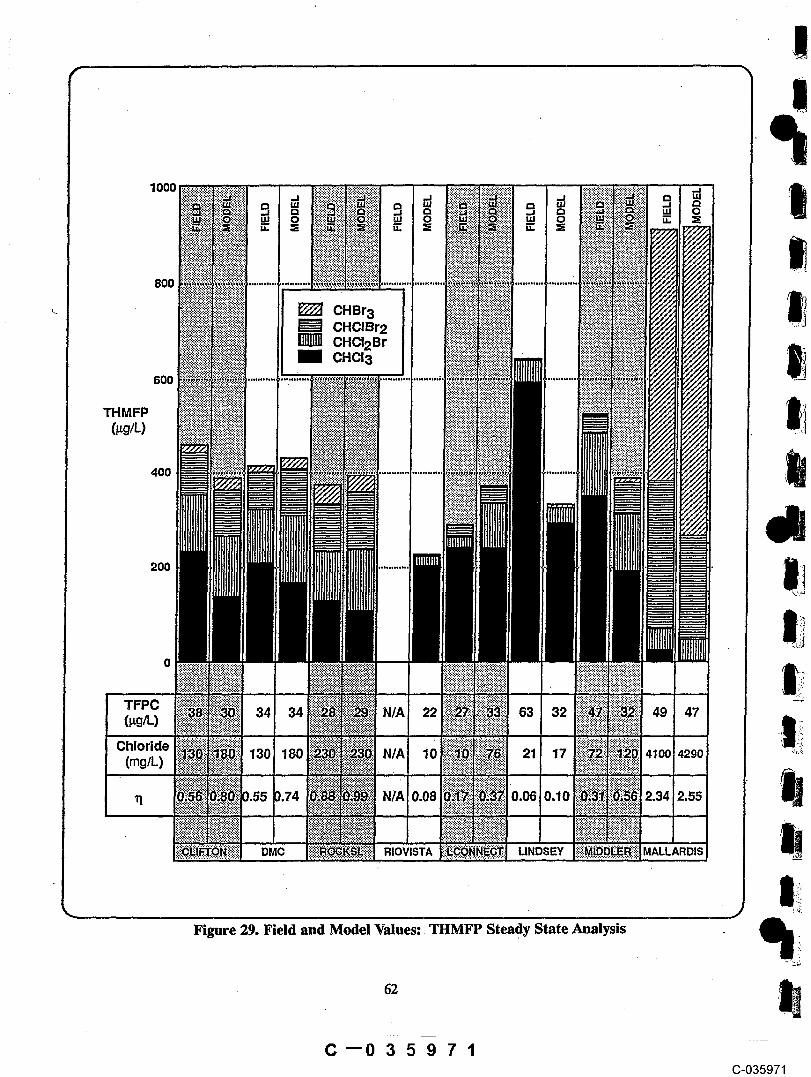
I

lOOO-I

0 u~ 0 0

800 .~.’~.~:.’-:.,.~., ........

~ CHBr3~ CHCIBr2~ CHCI2Br~ CHCl3

6oo

THMFP

400

200 IIIIIIIii

o tTFPC ~2(l~g/L)

Chloride ~’~(rag/L)

11 10

DMC RIOVISTA LINDSEY MALLARDIS

Figure 29. Field and Model Values:. THMFP Steady State Analysis

62

C--035971C-035971

Both TFPC and chloride predictions compare poorly with observed values at MIDDLER. However, THMFPestimates appear to be more sensitive to the deviation in TFPC than in chloride, as shown by the relatively pooragreement between chloroform concentrations and relatively good agreement between bromomethaneconcentrations. The overprediction of chloride at MIDDLER is attn’butable to DWRDSM, as the TDS to chloriderelationships was valid for this observation. Because TFPC is underpredicted rather than overpredicted, thisdeviation is probably a result of incomplete agricultural drainage description rather than a problem withDWRDSM.

||

C--035972C-035972


C--035973(3-035973

CHAPTER 9. FUTURE DIRECTIONS

The THMFP model framework, as presented in Chapter 5 and developed in Chapters 6 and 7, was applied to sevensimulation scenarios in Chapter 8. This exercise illustrated the model’s ability to quantify relative contributions ofTI-IM precursors from various Delta inflows and also illustrated the model’s ability to simulate bromide effects inthe Delta. The exercise also revealed a number of directions that can be taken in the future to enhance the modelframework.

Enhanced Boundary Conditions

Boundary conditions required by the Sacramento--San Joaquin THMFP model depend on the selected mode ofanalysis. For example, to simulate historic THM precursor transport in steady state or time series modes, chlorideand TFPC boundary conditions should be based on observed data for the period of interest. The problempresented in Chapter 8 is an example of simulating historic THM precursor transport in a steady state mode. Tos.imulate THM precursor transport in a planning mode, ’~oase" hydrologic and water quality conditions can bedeveloped from historic records to represent various year types and seasons. ~ "

Simulating THM precursor transport in a predictive or real-time mode with the existing fi~odel formulation isproblematic in regard to establishing boundary conditions. As discussed in Chapter 5, TFPC (the model parameterrepresenting precursor effects) cannot be estimated a priori but must be calculated from observed THMFPmeasurements. But by establishing relationships between TFPC and directly measurable water quality andhydrologic parameters at the boundaries, the ~odel can potentially be used in a predictive mode. In the past,DWRDSM has not typically been run in a predictive mode because of uncertainties associated with prototypegeometry, boundary conditions, and mixing charact .eristics. Potential refinements in the descriptions of agriculturaldrains and other botmdary conditions are proposed below.

Agricultural Drain Boundary Conditions

The simulation results presented in Chapter 8 highlight the need for a better description of precursor contributionsfrom agricultural drains. Deviations between predicted and observed values of THMFP were greatest at stations

limitation of the current THMFP model formulation. In addition to expanding the MVCQI monitoring program toinclude a larger number of agricultural drains, an effective model enhancement would be to develop amathematical description of precursor movement on Delta islands.

THMFP from agricultural drains appears to be related to soil type and degree of water saturation of the soil.1

These factors are also considered to be important in predicting agricultural drain salinity. Therefore, an existingDWRDSM drainage salinity submodel5° could be modified to simulate TFPC formation and transport from Deltaislands. A preliminary revision to the numerical formulation is presented in Eq. 9-1 of Fig. 30.

In E.q. 9-1, the impact of soil type on drainage quality is primarily represented by a term CSi, the maximum TFPCconcentration for a particular island soil. The DWRDSM drainage salinity submodel defines CSi as an averagesalinity for a particular island soil, a value that varies by the mechanisms of salt accumulation and leaching.. Whendescribing TFPC, CSi values should be higher for peat soils and lower for mineral soils. CSi could be utilized as acalibration factor in a drainage TFPC submodeI.

Soil type is also represented by the term fl, the leaching efficiency factor. This factor is assumed to vary between0.2 for clay soils and 0.6 for sandy soils in the DWRDSM drainage salinity submodel. The impact of soil saturationon drainage quality is primarily represented by the term f2, the drainage activity factor. This term is a cal~rationfactor in the DWRDSM drainage salinity module and is correlated with precipitation. The product of the leachingefficiency factor and the drainage activity factor is defined by the term f in Eq. 9-1. As f approaches its maximumvalue of 1, drainage quality is influenced mainly by soil type and, approaches a maximum value of CSi. As fapproaches its minimum value of 0, drainage quality is influenced mainly by irrigation qual!ty and approaches aminimum value of Ci.

C--035974C-035974

DIVERSION, ~ RETURN

Drainage WaterApplied Water Leach Drainage Qd’ CdLeach Water ET Precip Surface Runoff

,.. . " " :,:.. ". .: .." .’.. .- ..: :.S~p g~ " ’ ’ ’¯ :~= . : a . ¯ ¯ .-" ~: ¯ S6il I~lois’t~J~e ’" :::.!’:" ¯¯ .,:’

:/...~:::......~:..:..:.. tl:’owlands) ":::,,.,.......... , .. ....: ,:.. .....o’: .:...... "..’...... :.; ~.::- ..,. , : ....... .. : ¯ . .-... , ..., .... ¯ .-...::.:.~ % : :: ..,’.~,..:" ¯ .,

.:" ¯ " ....’::"- " " " :’:"":

MATHEMATICAL FORMU LATION

ct+l ~.d = fxCSi+ (l’f)xCt i ......... (9-1)

WHERE:

C d = Average TFPC concentration in return water

C$i = Maximum TFPC concentration in soil

C i = Average TFPC concentration in diversion water

f = flx f2 < 1

fl = Leaching efficiency factor

f2 = Drainage activity factor

Figure 300 TFPC Contributions from Agricultural Drainage

C--035975C-035975

Other Boundary Conditions~

~.A~ Ideally, TFPC boundary conditions could be specified as a multivariate function similar to Eq. 5-3 developed byAmy et aL29 Given DWR’s fixed reaction conditions (chlorine dose, time, temperature) and reported insensitivityto bromide,29 modified relationships could be developed as functions of UVA, TOC, pH, and chlorine residual.This latter term may include inorganic as well as organic demands. Unfortunately, the existing MWQI data base isnot adequate to develop such correlations. Instead, a simplified formulation was developed to ~estimate TFPC as afunction of TOC and average hydrology at key boundaries. This preliminary procedure is outlined below (see Fig.31) using the San Joaquin River at Vernalis as an example boundary:

1. Specify a flow rate and TOC concentration at the bounda.ry. Historic daily monthly average flow values arereadily available from DAYFLOW.49

2. Predict molar chloride concentration at the boundary from an established flow-salinity relationship:

In [C1-] = 6.69-0.758 lnQ .......................................................................(9-2)

where chloride concentration is in mM and flow is in cfs.

3. Calculate Bromine Incorporation Factor from the following location-specific empirical relationship:

3[Ct-]

ir/ -- 19.98 + [CI-] ..................................................................... (9-3)

4. Calculate the THMFP concentration of one "II-IM compound as a function of TOC and chloride. At Vernalis,the best ftmctional relationship was found with the compound CHCI2Br:

[CHCI2Br] -- 0.228 TOC0-340 [CI-]0-659 ........................................................... (9-4)

where:

CHC12Br and TOC concentrations are in gM and rag/L, respectively.

5. Calculate the distribution factor associated with the THMFP concentration determined in Step 4. Empiricalrelationships were developed in Chapter 7. For CHCI2Br,

-.0446~- .1888r/2 + .8659q............................................................. (9-5)

6. Divide the THMFP concentration calculated in Step 4 by the distn~bution factor calculated in Step 5 to arrive atthe TFPC concentration. For the Vernalis example,

[TFPC]. = [CHCI2Br]sl .................. , .......................................................(9-6)

C ~0 3 5 9-~-6C-035976

STEP 2: FLOW-SALINITY RELATIONSHIP STEP 3: BROMINE INCORPORATION FACTOR

I ! : ! ! : ’. :’.l ........ I I ’ ’ I I I .I II@ -’:. ............. ": ....... :."’"".’"":"~:.":.":."~’} .............. : ....... ’.’"’’,’"’~.’"~":."~’"."~" 1 ¯ ~5 ........................................................................................................

-..i ..............! .......~.....~...~...i..i..~..~.~ .....................~.....~.-..!...i..i..i+~:- .

~",’i"’""i""’~’"~’"i"i"~"ii .............~. .......!’""!"’i’i"i"i’~’i’" ~. ~ ........................................................................................................~ .....:..~. "~..o..:..o...~....;....~..;...;...’...’.. .............

~. .......;......~.....~...L.:...:..÷.’... .

""~ .............~ ......""’~’"’:’":"’:"’:"~’! .............T .......":’""’:’"’~’"~"~’’.’T’~" " "~ =. :. " ; " "- ~ ~ ~:.i :. ! :. ~ ~ ~ ~!~ @°9 ......................................................................................................

,., 1 -.= ..............." .......:...’".’o..:...=....:..::. ............. ".. .......:.....:....=...:o.:..:..:.:.. 11-.~ ..............

~. ....... ~.o.o.G..~..G,~.".~,.; °..’. .......... ÷ ....... ~°....:.....:....:. ..;...:..G:.."~ ...~ ..............",. ....... ~,....~:...=....~..G~,..~,.;. ..... .’..,..~.......G....~...-~..oi..~..~..~..:..0 8.6

.................. ¯ : .......!.....~. ...~...}..~..~..~.~ .....................~.....~....~...~, ..~..:.~.~. .

"" ~ ’i ..............! .......}""T’!’"!"!"!"!’i .......... ;"T .......};,!’"T"!"!"!’T’;"

G~ (cfs) [CI-] CmH)

STEP 4: THMFP SPECIES CONCENTRATION" STEP 51 BROMINE DISTRIBUTION FACTOR~1~

I .... ~ ’ ’ ’ ~ ’ ’ ’ ’ ~ ’ ’ ’ ’ ’ ’" ’ I ’ ’ ’ ’ ~ !’ ’ " ’ ’ ’ ’ " ’ ’ ’ ’

"° ..................................i ...............................................i ............: ..... ....................................................................................................--TOC -~ 2 mc~/L :

~..:

*’~ "i ....................... i ........................ i ....................... i’~: .............. !’

~ .i .........................................,......i....::S....-...k..-’..-. .........:. ...............-=~,~ ~)~ ~) :. :..° .~-: :~.....~ ..> .:....... .........................................

OJ "’"’"’~’’-:- ~ ~ ~ ¯ ..~| i :~~ s, 6 .... . ~ ................ ~ .....................

¯ ,~ : ." ..... : : - i ~ , , i i° -i .’..

,’~¢ ¯ i ~ , ! ! i e, ±~ o ;3 ""’~’"’"’"’"! .......................................... :"

I , . , . I o . , , I .... I .... 4 . . , . I , . , . I I . . ¯ I ..... , , I

I: C.I.- .I etcH)

Figure 31. Boundary Conditions at Vernalis

68

C--035977C-035977

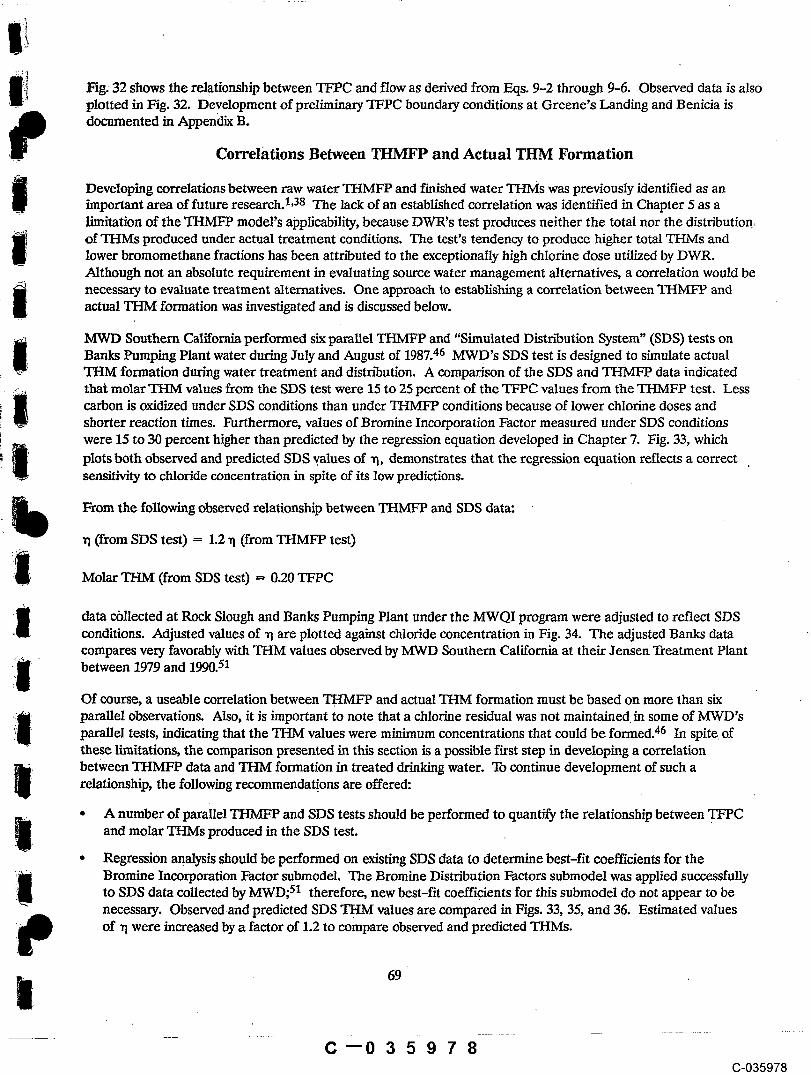
Fig. 32 shows the relationship between TFPC and flow as derived from Eqs. 9-2 through 9-6. Observed data is alsoplotted in Fig. 32. Development of preliminary TFPC boundary conditions at Greene’s Landing and Benicia isdocttmented in Appendix B.

Correlations Between THMFP and Actual THM Formation

Developing correlations between raw water THMFP and f’mished water THMs was previously identified as animportant area of future research.1,38 The lack of an established correlation was identified in Chapter 5 as alimitation of the THMFP model’s applicability, because DWR’s test produces neither the total nor the distribution,of THMs produced under actual treatment conditions. The test’s tendency to produce higher total THMs andlower bromomethane fractions has been attn’buted to the exceptionally high chlorine dose utilized by DWR.Although not an absolute requirement in evaluating source water management alternatives, a correlation would benecessary to evaluate treatment alternatives. One approach to establishing a correlation between THMFP andactual THM formation was investigated and is discussed below.

NIWD Southern California performed six parallel THMFP and "Simulated Distribution System" (SDS) tests onBanks Pumping Plant water during July and August of 1987.46 MWD’s SDS test is designed to simulate actualTHM formation during water treatment and distn"oution. A comparison of the SDS and THMFP data indicatedthat molar THM values from the SDS test were 15 to 25 percent of the TFPC values from the THMFP test. Lesscarbon is oxidized under SDS conditions than under THMFP conditions because of lower chlorine doses andshorter reaction times. Furthermore, values of Bromine Incorporation Factor measured under SDS conditionswere 15 to 30 percent higher than predicted by the regression equation developed in Chapter 7. Fig. 33, whichplots both observed and predicted SDS values of -q, demonstrates that the regression equation reflects a correctsensitivity to chloride concentration in spite of its low predictions.

From the following observed relationship between THMFP and SDS data:

~1 (from SDS test) = 1.2 ~1 (from THMFP test)

Molar ~ (from SDS test) -- 0.20 TFPC

data cbllected at Rock Slough and Banks Pumping Plant under the MWQI program were adjusted to reflect SDSconditions. Adjusted values of ~ are plotted against chloride concentration in Fig. 34. The adjusted Banks datacompares very favorably vdth THM values observed by MWD Southern California at their Jensen Treatment Plantbetween 1979 and 1990.51

Of course, a useable correlation between "I!-I. MFP and actual THM formation must be based on more than sixparallel observations. A/so, it is important to note that a chlorine residual was not maintained, in some of MWD’sparallel tests, indicating that the THM values were minimum concentrations that could be formed.46 In spite ofthese limitations, the comparison presented in this section is a possible first step in developing a correlationbetween TI-1-MFP data and THM formation in treated drinking water. To continue development of such arelationship, the following recommendations are offered:

¯ A number of parallel THMFP and SDS tests should be performed to quantify the relationship between TFPCand molar THMs produced in the SDS test.

¯ Regression analysis should be performed on existing SDS data to determine best-fit coefficients for theBromine Incorporation Factor submodel. The Bromine Distribution Factors submodel was applied successfullyto SDS data collected by MWD;51 therefore, new best-fit coefficients for this submodel do not appear to benecessary. Observed.and predicted SDS THM values are compared in Figs. 33, 35, and 36. Estimated valuesof ~1 were increased by a factor of 1.2 to compare observed and predicted THMs.

C--035978C-035978

Figure 32. Flow-TFPC Relationship at Vernalis

70C--035979

C-035979

Figure 33. Banks Pumping Plant SDS Tests

71

C--035980C-035980

Banks Pump£ng P1ant

~o ~5 .................................................................................. :. .........................................................................................................................- "4"

+.,~..~,~..;.* ...................................................................................................................+ +

++

=.s ....................................................... +,� ................................................................ ; .............................................................................+ +

+.... ~ ........................ +...~.,...~.~..: ................................................................................................................... ~ ...........................................

~, ~ ....] ..........~+..~@ ................... ~ ............. =. ..............~....~..~ ...............L- ....................................................... ~ ...........................................

.-: ~ -. ~

.

+~, ~ .................................................................................................................. ~...~.~.....~. ............ ~. ............. : ...................................... : ....

+++ +

*~...~ ............................................................................

**+

~**~ ** .~ ¯ ~ ¯ ".... L....~..~.~.~ .., ...............~ .................................L.k ......:; ........: ...................~ .....................................~ .............................

~ .... ~ ............................................................................. ~ ............................ ~ ......... ~ ...................................... ~ ...........................................

g ~ 4 6 8

Figure 34° THMFP Data Adjusted to SDS Conditions

?2

C--035981C-035981

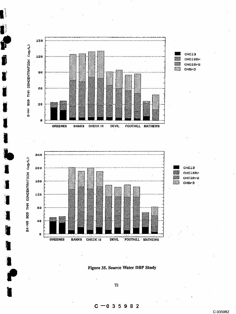
~ CHCIO

~ ~ CHCI2~ro ~ CHCZS~H

~ ~ CHBr3~ ~ ............................. ,

Z

Z0 6~ .............................

I

i GREENES BANKS CHECK 13 DEVIL FOOTHILL MATHEWS

|

~ CHCIRB~~ CHCIBr2~ CHBr~

o

| ,GREENES BANKS CHECK 13 DEVIL "~: FOOTHILL ~ MATNEWS

|Figure 35. Source Water DBP Study

73

C--035982C-035982

3an i99~ L~ve Oak Reservoir Stud~

248

~ CHOIBr~~ CHef3

B~ (mg/L) 0.45 0.45 0.45 1.35 1,35 1.35 1o35Cl2 (ppm) 3 4 5 3 4 5 6

Aug LSge $D$ Tests

CHCI~

E CHCI2Br~’~ CHC~B~

~] CHBr3

GREENES BANKS CHECK 13 GREENES BANKS CHECK13

Figure 36, Other SDS Studies

74

C--035983(3-035983

Multi-Constituent Transport

Seven DWRDSM runs were made to illustrate the model methodology in Chapter 8. Of these seven ruris, fivesimulated the transport of TFPC from different boundaries, one simulated the cumulative effect of TFPC from allboundaries, and one simulated the cumulative effect of chloride from all boundaries. The information from theseseven DWRDSM runs could be reproduced in one run by modifying the model to route several conservativeconstituents simultaneously. For the analysis of THMFP in the Delta, conservative constituents would includechloride and TFPC from five major independent sources (Sacramento River, San Joaquin River, Benicia, PeatIsland drainage, and Mineral/Intermediate Organic Island drainage). Multi-c.onstituent t.ransport would saveconsiderable model analysis time.

Coordinated Data Collection and Analyses

The preliminary modeling have emphasized importancecoordination betweenefforts the of theDivisionof LocalAssistance and the Division of Planning. As the model is refined and caI~rated with additional data, it willcontinue to provide better guidance in planning the MWQI monitoring program. Model sensitivity analysis canplay a key role in establishing data collection priorities. This link between model analysis and data collection willrequire an even closer coordination between the two Divisions in the future.

Management Alternatives Evaluation

When further confidence is gained with the THMFP model calibration, a variety of water quality managementalternatives can be evaluated. For example, benefits of new tidal barriers, variable pumping schedules, andregulated agricultural drainage can be evaluated and quantified.

To illustrate the evaluation of management alternatives, a simple problem is presented below. The problem wasdefined so that no DWRDSM runs were required. No conclusions should be drawn from this illustration.

Hypothetical Problem Definition

Due to concerns with THMs in treated water from the Delta, salinity barriers are strategically placed so thatreverse flow into the Delta from the Bay is greatly reduced. The resulting water quality impact is as follows:bromide concentration is reduced from 0.51 mg/L (150 mg/L chloride) to 0.17 mg/L (50 mg/L chloride). How muchis THMFP reduced at Clifton Court Forebay by this action?

Hypothetical Problem Assumption

The intent of the management alternative is to minimize reverse flow into the Delta from the Bay. It is assumedthat this alternative impacts the bromide load but has little impact on the organic precursor load at Clifton CourtForebay. This assumption is based on the DWRDSM model results (Scenario 3)presented in Chapter 8, whichshows that Bay influences on TFPC transport are limited to the western Delta.

Marginal Benefit Calculations

Figs. 37a-3To show the marginal effects of controlling bromide on THMFP production, assuming TFPCconcentrations typically observed at Delta export stations. These curves were derived from the empiricalrelationships Bromide Incorporation Factor and Bromine Distrfaution Factors.

C--035984C-035984

|

i i I | i I I I I i I I I I"

:-

-,, "......

- - - rFP~=45 ug/L

Go ~e ....;o ........ ........¯ ....................~’-

~ ......., :~:~..... ............................................................................................................................................................................ ~ .....

. ", i "’’. ......... rFPQ=6G ug/L

~ i ~ "’-.

~ .." , "...

I Go 16 ............................................... . ..................... ~ ................... ’." ,: ........................................ ." .......................................... : .......................................... : .....L ~ : ¯ : -... : . : :

:E :" ~ " ".". "’L. :"

;i ..............................................................................~- ~ ....~ ..........................................~ ...........................................i .......................................................................: ..............i ..........................................~ .....

8.4 e.6 e.8 t,i

BROMZDE CONCENTRATTON (mg/L)

Figure 37a. Marginal Benefits of Bromide Control

C--035985C-035985

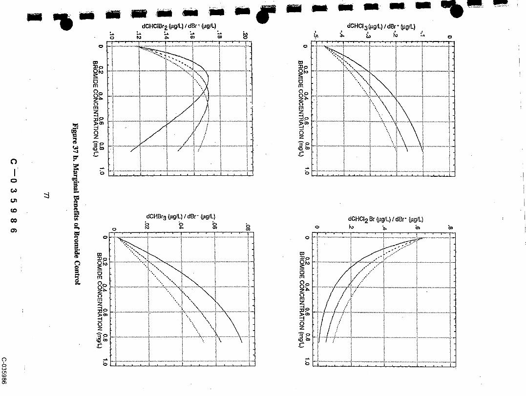
ITotal TI-IMFP. The folIowing linear relationship exists between average moIecular weight (AMW) and BromineIncorporation Factor (Vl) for the four THM species:

AMW (gg/gm01e) : 119.4 + 44.4~1 .......................................................(9-7) :

THMFP mass concentration is equal to the product of TFPC and AMW, yielding:

THMFP 0tg/L) = 119.4[TFPC] + 44.4-q[TFPC] ....................................................(9-8)

The pa,"tial derivative of THMFP with respect to [C1-] is the product of the partials: l !

O THMFP = O THMFP Orla [Cl-] an a [Ct’] ............................................................. (9-9)

where:

aTHMFP=44"4[TFPC] l~:Dr/ .................................................................... (9-10) ,

3b [TFPC]a [Cl’] (b [TFPC] + [el-])2 .... ~ ........................................................... (9-11)

Fig. 37a plots the 15artial derivative given in Eq. 9-9, modified to reflect mass bromide concentration instead ofmolar chloride concentration. The modification assumes a bromide to chloride mass ratio of 0.0034. This figuresuggests that in a typical Delta export salinity range of 0.17-0.85 mg/L bromide (50-250 mg/L chloride), themarginal benefit of reducing bromide by 1 p.g/L corresponds to a reduction in THMFP by approximately 0.1-0.2ttg/L.

CHCIa. By modifying Eq. 7-5, the mass concentration of CHCI3 can be defined as the product of so, TFPC molarconcentration, and CHCI3 molecular weight, or:

CHC13 (Isg/L) = 119.4[TFPC](c’q3 +~ drl2 +e~] +1) ............................................... (9-12)

where c,d, and e represent the regression coefficients in Eq. 7-9. The partial derivative of CHCI3 with respect to

[CI-] is the product of the partials:

~ CHCl3_ O CHCI3 ar/

a [ct’l an a [Cl’] ......................................... ~ ...................... (9-13)

where:

aCHCla = 119.4 [TFPC] (3cr/~+ 2dr/+e)

or/ ..................................................... (9-14)

and O [Cl’] is defined in Eq. 9-11.

78

C--035987C-035987

CHClzBr, CHCIBrz & CI-IBr3. The partial derivatives of the THMFP bromomethane species with respect to [CI-]can be developed in a manner similar to that presented for CHCI3, resulting in the following partials:

O CHC12Br- 163.8 [TFPC] (2cr/3+ dr/2+ 3cr/~+ 2 dr/+ e)

Or/ (r/+ 1)2 ...................................... (9-15)

3. CH�IBr~. = 208.3 [TFPCl (3cn2+ 2dr/+ e)~r/ ..................................................... (9-16)

O CI-1Br3. --252.7 [TFPC] (3cr/2+ 2dr/+ e)

0r/ ..................................................... (9-17)

Fig. 3713 plots the partial derivatives for each THMFP species with respect to [CI-], again modified to reflect massbromide concentration instead of molar chloride concentration. The figures suggest that in a typical Delta exportsalinity range of 0.17-0.85 mgfL bromide (50-250 mg/L chloride), the marginal effect of reducing bromide by 1 Isg/Lcorresponds to the following change in THMFP species distribution:

0.1-0.4 Isg/L increase in CFICI3

0.0-0.4 lsg/L decrease in CHCI2Br

0.1,-0.2 btg/L decrease in CHC1Br2

0.0-0.1 ttg/L decrease in CHBr3

The marginal benefit analysis presented in this example problem suggests that controlling bromide intrus.i0n intothe Delta results in a net reduction in THMFP. The net reduction in THMFP is accomplished through aredistnq3ution of THMFP species, with more chloroform and fewer bromomethanes produced.

THMFP Reduction Calculations

Table 6 summarizes the calculated THMFP values under base and plan conditions defined above. Themanagement alternative results in a reduction of total THMFP mass concentration by approximately 8 to 12percent. An even more important result is the change in THMFP species distn"oution between the base and planconditions. While chloroform increased by 26 to 50 percent, all bromomethane species decreased dramatically:CHCI2Br was reduced by 41 to 53 percent, CHC1Br2 was reduced by 70 to 71 percent, and CI-IBr3 was reduced by85 to 90 percent. As discussed throughout this report, THMFP data must be interpreted with an awareness thatthe test inherently produces higher total THMs and lower bromomethane fractions than produced under actualwater treatment conditions.

Table 6. THMFP: Base versus Plan Conditions30/~g/L TFPC 45 ~tg/L TFPC 60 ~g/L TFPC

base plan base plan base planCHCI3 153 230 279 374 413 520

CHC12Br ’~’23 ’ 72 159 81 184 87

CHC1Br2 83 25 82 24 79 23

CHBr2 18 2 13 2 10THMFP 376 330 532 481 686 631

Base Condition: Br- -- 0.51 mgiL (C1- -- 150 rag/L)Plan Condition: Br-= 0.17 rag/L (CI-= 50 rag/L) ..

C--035988(3-035988


C--035989C-035989

REFERENCES

1. California Department of Water Resources, Delta Island Drainage Investigation Report of the lnteragency DeltaHealth Aspects Monitoring Program, A Summary of Observations During Consecutive Dry Year Conditions, Water Years1987and 1988, June 1990.

2. DWR, Project Report of the Interagency Delta Health Aspects Monitoring Program: Summary of Monitoring Results1988-89, October 1990.

3. DWR, The Delta as a Source of Drinking Water, Monitoring Results, 1983 to 1987, August 1989.

4. Snoeyink, V.L and Jenkins, D., Water Chemistry, Wiley & Sons, New York, 1980.

5. Amy, O.L et al., "Evaluation of THM Precursor Contn~outions from Agricultural Drains," Journal AWWA, 82:1,1990.

6. DWR, "Delta and Suisun Bay Water Quality Investigation,~’ Bulletin 123, August 1967.

7. DWR, State Water Project Trihalomethane Study, April 1982.

8. Disma, D. et aI., "Supply of Suspended Matter and Particulate and Dissolved Organic Carbon from the Rhine tothe Coastal North Sea," SCOPE/UNEP Transport of Carbon and Minerals in Major World Rivers, Degens, E.T., ed.,52, University of Hamburg, Hamburg, 1982.

9. Laane, R.W., "Conservative Behavior of Dissolved Organic Carbon in the Ems-Dollart Estuary and the WesternWadden Sea," Netherlands 1ournal of Sea Research, 14, 1980.

10. Loder, T.C. and Hood, D.W., "Distribution of Organic Carbon in a Galacial Estuary in Alaska," Limnology andOceanography, 17, 1972.

11. Mantoura, R.E and Woodward, E.M., "Conservative Behavior of Riverine Dissolved Organic Carbon in theSevern Estuary: Chemical and Geochemical Implications," Geochimica et Cosmochima Acta, 47, 1983.

12. Moore, R.M. et aL, "The Behavior of Dissolved Organic Material, Iron and Manganese in Estuarine Mixing,"Geo6hemical et Cosmochicmica Acta, 43, 1979.

13. Sholkovitz, E.R. and Copland~ D., "The Coagulation, Solubility and Adsorption Properties of Fe, Mn, Cu, Ni,Co and Humic Acids in River Geochimica Cosmochimica 1981.Cd, a Water," et Acta, 45,

14. Gong, B. and Edzwald, J.K., Seasonal Evaluation of Organics Removal at a Conventional Water Treatment Plant,Proceedings 1981 AWWA Annual Conference, 1981.

15. Singer, P.C. et al., ’~I’rihalomethane Formation in North Carolina Drinking Water," JournalAWWA, 72:8, 1980.

16. Bunn, W.W. et aI., "Formation of Trihalomethane by Chlorination ofSurface Waters," Environmental Letters,10:3, 1975

17. Minear, R.A., Production, Fate and Removal of Trihalomethanes in Municipal Drinking Water Systems, ResearchReport No. 78, Tennessee Water Resources Research Center, Knoxville, "IN, April 1980.

18. Trnssell, R.R. and Umphres, M.D., "The Formation of Trihalomethanes," Journal AWWA, 70:11, 1978.

19. Lange, A.L. and Kawczynski, E., "Controlling Organics: The Contra Costa County Water District Experience,"Journal AWWA, 70:11, 1978.

C--035990(3-035990

20. Malcolm Pirnie, Inc., Review of THMFP Moael Development by CDWR, letter to MWD Southern California,February 4, 1991.

21. MWD Southern California, Delta Water Quality Issues, 9-11-90 office memorandum.

22. Jung, M., MWQI Bromide Monitoring Update, prepared for DWR, January 16, 1991.

23. Moore, G., TuthilI, R. and Polakoff, D., ’~A Statistical Model for Predicting Chloroform Levels in ChlorinatedSurface Water Supplies," Journal AWWA, 71:1, 1979.

24. Kavanaugh, M.C. et al., ’~m Empirical Kinetic Model of Tdhalomethane Formation: An Application to Meetthe Proposed THM Standard," Journal AWWA, 72:10, 1980.

25. Engerholm, B.A. and Amy, G.L., ’A Predictive Model for Chloroform Formation from Humic Acid," JournalAWWA, 75:8, 1983.

26. Urano, K., Wada, H. and Takemasa, T., "Empirical Rate Equations of Trihalomethane Formation WithChlorination of Humie Substances in Water," Water Research, 17:12, 1983.

27. Morrow, C.M. and Minear, R.A., "Use of Regression Models to Link Raw Water Characteristics toTrihalomethane Concentrations in Drinking Water," Water Research, 21:1, 1987.

28. Amy, G.L, Minear, R.A. and Cooper, W.J., ’~Testing and Validation of Multiple Non-Linear Regressed Modelfor Predicting Trihalomethane Formation Potential," Water Research, 21:6, 1987.

29. Amy, G.L., Chadik, Z.K. a~ad Chowdhury, Z.K., "Developing Models for Predicting Trihalomethane FormationPotential Kinetics," Journal AWWA, 79:7, 1987.

30. Amy, G.L et al, ’~A Mathematical Model for Trihalomethane Formation in a Highly Colored GroundwaterContaining Ammonia and Bromide," Preprints Div. Envir. Chem. Amer. Chem. Soc., 23:171, 1983.

31. Lnong, T., Peters, C. and Perry, R., "Influence .of Bromide and Ammonia Upon the Formation ofTrihalomethanes Under Water Treatment Conditions," Envir. Sci. & TechnoL, 16:473, 1982.

32. Khordagui, H., Stochastic Prediction of Trihalomethane Production in Chlorinated Drinking Water, DoctoralDissertation, University of Michigan, Ann Arbor, 1982.

33. Edzwald, J.K., Becker, W.C. and Wattier, K.L., "Surrogate Parameters for Monitoring Organic Matter andTrihalomethane Precursors," Journal AWWA, 77:4, 1985.

34. Singer, P.C. and Chang, S.D., "Correlations Between Trihalomethanes and Total Organic~ Halides FormedDuring Water Treatment," Journal AIYWA, 81:8, 1989..

35. Reckhow, D.A. and Singer, EC., "By-Products in Drinking Water: From Formation Potentials to Finished WaterConcentrations," Journal AWWA, 82:4, 1990.

36. Reckhow, D.A. and Edzwald, J.K., "Bromoform and Iodoform Formation Potential Tests as Surrogates forTrihalomethane Formation Potential," Journal AWWA, 83:5, 1991. ~

37. Singer, EC., Trihalomethane Formation Potential, The Search for a Surrogate, AWWA R~searchFoundation/KIWA, October 1988.

38. California State Water Resources Control Board, Water Quality Control Plan for Salinity, Final Draft, January

82

C--035991C-035991

39. Fischer, H.B., A Lagrangian Method for Predicting Pollutant Dispersion in Bolinas Lagoon, Matin Coup,California, US Geological Survey Paper 582-B, 1972.

40. Fischer, H.B., a~ischer Delta Model, Volume 2: Reference Manual~ Report I-IBF-84/01, Hugo B. Fischer, Inc., 1984

41. DWR, Methodology.for Flow and Salinity Estimates in the Sacramento-San doaquin Delta and San Francisco Bay,12th Annual Progress Report to SWRCB, April 1991.

42. Evenson, D. and Johnson, A., Parameter Estimation Program: Program Documentation and User’s Manual, WaterResources Engineers, Inc., 1975.

43. Barnes, G.W. and Chung, F.I., "Operational Planning for California Water System," ASCE Journal of WaterResources Planning and Management, 112:1, 1986.

44. Gould, J.P., Fitchhom, L.E. and Urheim, E., "Formation of Brominated Trihalomethanes: Extent andKinetics," Water Chlorination: Environmental Impacts and Health Effects, Vol. 4, .lolley, R.L et al., Eds., Ann ArborScience, 1981.

45. Rebhun, M., Manka, J. and Zilberman, A., ’¢Frihalornethane Formation in High-Bromide Lake Galilee Water,"Journal AWWA, 80:6, 1988.

46. MWD Southern California, Bromide Incorporation in THMs, 2-1-91 office memorandum.

47. DWR, Salinity Unit Conversion Equations, 6-24-86 office memorandum.

48.DWR, Sacramento-San Joaquin Delta Water Quality Surveillance Program - 1988: Volume 1, May 1990.

49. DWR, DAYFLOW Program Documentation and DAYFLOW Data Summary: Users Guide, February 1986.

50. DWR, Agricultural Drainage Model, September 1990 (DRAFT).

51. MWD Southern California, SDS Data Delta 2-27-91 memorandumDWR.on Waters, to

C--035992(3-035992


C--035993C-035993

APPENDIX A

REVIEW OF DWR’S THMFP MODEL - G. AMY

|

C--035994C-035994

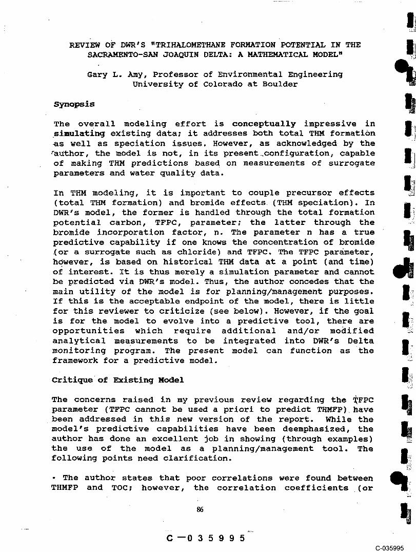
REVIEW OF DWR’S "TRIHALOMETHANE FORMATION POTENTIAL IN THE"I~ii~SACRAMENTO-SAN JOAQUIN DELTA: A MATHEMATICAL MODEL" ~

Gary L. Amy, Professor of Environmental EngineeringUniversity of Colorado at Boulder

Synopsis

The overall modeling effort is conceptually impressive in.simulating existing data; it addresses both total THM formationas well as speciation issues. However, as acknowledged by the~Uthor, the model is not, in its present.,configuration, capableof making THM predictions based on measurements of surrogateparameters and water quality data.

In THM modeling, it is important to couple precursor effects(total THM formation) and bromide effects. (THM speciation). InDWR’s model, the former is handled through the total formationpotential carbon, TFPC, parameter; the latter through thebromide incorporation factor, n. The parameter n has a truepredictive capability if one knows the concentration of bromide.(or a surrogate such as chloride) and TFPC. The TFPC parimeter,however, is based on historical THM data at a point (and time)of interest. It is thus merely a simulation parameter and cannotbe predicted via DWR’s model. Thus, the author concedes that themain utility of the model is for planning/management purposes.If this is the acceptable endpoint of the model, there is littlefor this reviewer to criticize (see below). However, if the goalis for the model to evolve into a predictive tool, there areopportunities which require additional and/or modifiedanalytical measurements to be integrated into DWR’s Deltamonitoring program. The present model can function as theframework for a predictive model.

Critique~of ExistingModel

The concerns raised in my previous review regarding the ~,FPCparameter (TFPC cannot be used a priori to predict THMFP). havebeen addressed in this new version of the report. While themodel"s predictive capabilities have been deemphasized, theauthor has done an excellent job in showing (through examples)the use of the model as a planning/management tool. Thefollowing points need clarification.

¯ The author states that poor correlations were found betweenTHMFP and TOC; however, the correlation coefficients ¯ (or

C--035995C-035995

coefficients of determination) associated with Figures 2 and 3are not reported. With the elimination of a few outliers, thesecorrelations seem fair. I would maintain that a r2 ofi forexample, 0.8 would be reasonable as a predictive tool forobtaining approximations.

- The correlation coefficient (or coefficient of determination)~or Equation 4-4, showing.br0mide as a function of chloride,should be indicated.

¯ Equation 7-1 in Figure 6 is misnumbered.

¯ For the relationships shown in Table i, the linearizationtechnique and the linear forms should be indicated. Since r2values pertain to linearized forms, it should be noted that, inthe case of transformed ~variables, r2 requires carefulinterpretation.

¯ As indicated by the author, submodel # 3 in Table 1 mimicksthe mathematical definition of n. However, it provides thepoorest correlation of data. Since n does not linearly withvaryCl- (Br-), there is clearly an asymptotic behavior as napproaches 3.0 at high Cl- (Br-).~ The relationship selected,submodel # 5, makes theoretical sense because it indicates theimportance of the Br-/TOC ratio in influencing THM speciation.

¯ The example shown on page 35 is somewhat curious. The problemstatement includes an assumed TFPC of 30 ug/L, based on somehistorical THM data. The problem then proceeds to "predict" THMspecies. How do the predictions compare with the data used toestimate TFPC in the first place? I realize that bromide (n) isalso influential but it wou~d be interesting to compare the twosets of THM values.

Future Directions

The TFPC parameter represents a measure of the organic carbonwhich becomes incorporated into THM species; thus, a measurementof the four species along with molecular weight relationshipspermits its calculation. Since on a molar basis, TFPC carbon andTHMFP are equal; it might be less confusing and more appropriateto simply use the latter terminology (i.e., molar-THMFP) withinthe model. The TFPC parameter really gives no insight intoprecursor character but rather merely describes observations ofmolar-THM formation without any measurements of the amount andcharacter of organic-precursor present in that sample. If THM

C--035996C-035996

data for its calculation did not exist, one would expect TFPC(or molar-THMFP) to be a function of the total amount of organicmatter (TOC), the character of the organic matter (e.g., humiccontent), and water quality conditions (e.g., pH).

DWR should strive to develop a means of predicting (as opposedto measuring) TFPC (or molar-THMFP). The necessary independentparameters should reflect organic-precuror characteristics andbromide, as well as influential water quality parameters such as

for TFPC are for source-specific correlations (e.g., SacramentoRiver, San Joaquin River, agricultural drains). The hydrodynamicfeatures of the present model configuration would allowassessment of the transport of different-character precursorsthrough the Delta.

Whereas TOC alone may not be an adequate surrogate parameter forTFPC (or molar-THMFP), multiplicative parameters (e.g., amultiplicative function of TOC and UV absorbance) may providemore accuracy. Another easy-to-measure surrogate parameter isfluorescence.

DWR should reexamine the way it performs THMFP tests. There aretwo alternative approaches: (i) based on a specifiedchlorine/total organic carbon (CI2/TOC) ratio (e.g., 3mg/img) or(ii) based on the chlorine dose required to provide a targetresidual (e.go, 0.5 to 1.0 mg/L) at the end of the designatedreaction time frame. The use of an arbitrarily high chlorinedose (120 mg/L) causes two problems: (i) it provides an unequal"driving force" for low versus high precursor samples and (ii)it understates the magnitude of brominated THMs..DWR’s test alsouses ambient pH; differences of +/- one pH unit cansignificantly affect THM formation. Also, my understanding~isthat DWR does not quantitatively measure chlorine residualwhich, if done, would permit a determination of chlorineutilization/demand. Beyond FP tests, there is much meri~ tosimulated distribution system (SDS) tests, based on lowerchlorine doses (e.g., CI2!TOC = I:i) and shorter reaction times~(e,g., 24 hours). The merits of these tests are two-fold: ..(i)they are more representative ~of actual water distributionsystems and (ii)the magnitude of brominated species is moreaccurately represented. Some utilities have developed goodrelationships between either SDS~THMs or actualdistribution-system THMs and THMFP; typically, the ~former has

88

C--035997(3-035997

been found to be about 25 to 50 % of the latter. This endeavor,however, has been limited to utility-specific correlations.

The large amount of chlorine used in DWR’s THMFP tests favorsmore chloroform formation; also, the long reaction time frameprovides for more chloroform formation since the formationkinetics for bromoform and brominated species are more rapidthan those for chloroform.

THM speciation is important for two reasons: (i) recent healthevidence suggests that bromodichloromethane may represent a~higher risk than other THM species and (~ii) brominated speciesmake it more difficult to meet a weight-based (ug/L) MCL.(Expressing concentrations as molar-based dampens the "chemical"role of bromide).

Future Data Needs

Through its Delta monitoring program, DWR could develop aninventory of precuror and actual bromide levels throughout theDelta. Sample locations should include major inflows, outflows,relevant transects between inflows and outflows, andagricultural drains. Precursor parameters could include DOC, UVabsorbance, fluorescence, THMFP, and SDS-THMs. Other waterquality parameters such as pH should be included. Ifquantitative measurements of chlorine residual are made, thiswould provide of calculating chlorinea meansutilization/demand. The resultant data base would permitidentification of: (i) multivariate correlations for TFPC(molar-THMFP) and .(ii) correlations between’ TKMFP and sDS-THMswhich would provide~ insight into actual distr.ibution-systemTHMs o

In any~ future modeling (reformulation, recalibration), therelationships involving n may have to be modified. The n factoris ¯based on TFPC results derived from the present THMFPprotocol.

!

C--035998(3-035998


C~035999(3-035999

APPENDIX B

ESTIMATING TFPC AND CHLORIDE BOUNDARY CONDITIONS

C--036000(3-036000

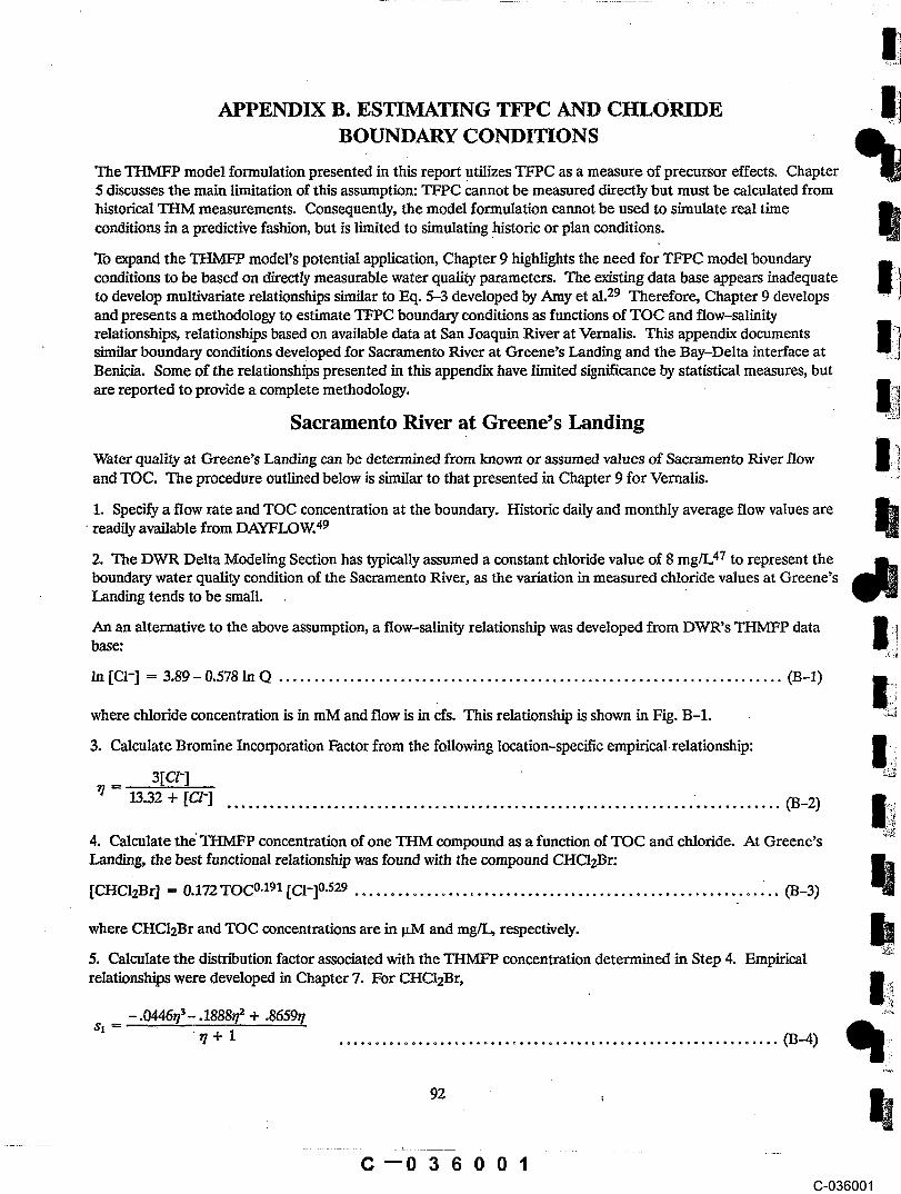
APPENDIX B. ESTIMATING TFPC AND CHLORIDEBOUNDARY CONDITIONS

The THMFP model formulation presented in this report utilizes TFPC as a measure of precursor effects. Chapter5 discusses the main limitation of this assumption: TFPC cannot be measured directly but must be calculated fromhistorical THM measurements. Consequently, the model formulation cannot be used to simulate real timeconditions in a predictive fashion, but is limited to simulating .historic or plan conditions.

To expand the THMFP model’s potential application, Chapter 9 highlights the need for TFPC model boundaryconditions to be based on directly measurable water quality parameters. The existing data base appears inadequateto develop multivariate relationships similar to Eq. 5-3 developed by Amy et al.29 Therefore, Chapter 9 developsand presents a methodology to estimate TFPC boundary conditions as functions of TOC and flow-salinityrelationships, relationships based on available data at San Joaquin River at Vernalis. This appendix documentss~milar boundary conditions developed for Sacramento River at Greene’s Landing and the Bay-Delta interface atBenich. Some of the relationships presented in this appendix have limited significance by statistical measures, butare reported to provide a complete methodology.

Sacramento River at Greene’s Landing

Water quality at Greene’s Landing can be determined from known or assumed values of Sacramento River flowand TOC. The procedure outlined below is similar to that presented in Chapter 9 for Vernalis.

1. Specify a flow rate and TOC concentration at the boundary. Historic daily and monthly average flow values arereadily available from DAYFLOW.49

2. The DWR DeIta Modeling Section has typically assumed a constant chloride value of 8 mg/L47 to represent theboundary water quality condition of the Sacramento River, as the variation in measured chloride values at Greene’sLanding tends to be small.

base:An an alternative to the above assumption, a flow-salinity relationship was developed from DWR’s THMFP data

In [C1-] -- 3.89 - 0.578 In Q ......................................................................(B-l)

where chloride concentration is in mM and flow is in ~fs. This relationship is shown in Fig. B-I.

3. Calculate Bromine Incorporation Factor from the following location-specific empirical, relationship:

3[Ct-]~/= 13.32 + [CI-] ........................................................................... 03-2)

4. Calculate the TI-EVIFP concentration of one THM compound as a function of TOC and chloride. At Greene’sLanding, the best functional relationship was found with the compound CHClzBr:

[CHCI2Br] = 0.172TOC0"191 [CI-]0-529 ........................................................... 03-3)

where CHCI2Br and TOC concentrations are in p.M and rag/L, respectively.

5. Calculate the distn’bution factor associated with the THMFP concentration determined in Step 4. Empiricalrelationships were developed in Chapter 7. For CHC12Br,

-.0446 3- .1888 /2 + .8659r/~ + 1 ............................................................. 03-4)

92

C--036001C-036001

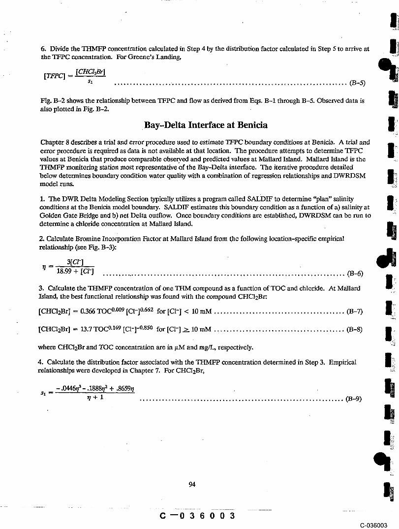
6. Divide the THMFP concentration calculated in Step 4 by the distribution factor calculated in Step 5 to arrive atthe TFPC concentration. For Greene’s Landing,

[TFPC] = [CHCI2Br]sl .................. , ................................~ ......................03-5)

Fig. B-2 shows the relationship between TFPC and flow as derived from Eqs. B-1 through B-5. Observed data is ~also plotted in Fig. B-2.

, Bay-Delta Interface at Benicia !i

Chapter 8 descn~oes a trial and error procedure used to estimate TFPC boundary conditions at Benicia. A trial and

error procedure is required as data is not available at that location. The procedure attempts to determine TFPCw ,i.values at Benicia that produce comparable obse .ryed and predicted values at Mallard Island. Mallard Island is theTHMFP monitoring station most representative of the Bay-Delta interface. The iterative procedure detailedbelow determines boundary condition water quality with a combination of regression relationships and DWRDSMmodel runs.

1. The DWR Delta Modeling Section typically utilizes a program called SALDIF to determine "plan" salinityconditions at the Benicia model boundary. SALDIF estimates this boundary condition as a function of a) salinity atGolden Gate Bridge and b) net Delta outflow. Once boundary conditions are established, DWRDSM can be run todetermine a chloride concentration at Mallard Island. ~l

2. Calculate Bromine Incorporation Factor at Mallard Island from the fo!lowing location-specific empiricalrelationship (see Fig. B-3):

3[cz-]’~ = 18.99 + [cl-] ............................................................................. 03-6)

3. Calculate the THMFP concentration of one THM compound as a function of TOC and chloride. At MallardIsland, the best functional relationship was found with the compound CHC12Br:

|[CHCI2Br] -- 0.36~ TOC°.~ [CI-]~.aa~ for [Cl-] < i0 mM 03-7) ....

[CHC12Br] - 13.7 TOC0.169 [C1-]-°.850 for [CI-] ~ 10 mM., ....................................... (B-8)

where CHCI2Br and TOC concentration are in gM and rag/L, respectively.

4. Calculate the distribution factor associated with the THMFP concentration determined in Step 3. Empiricalrelationships were developed in Chapter 7. For CHC12Br,

-.0446~-.1888rf + .8659r/,~+ 1 ................................................................03_9)

C-036003

l i i II I I i iI

iiiii i ! ii ~

i .1.lli~ " .................................... f .................. -’: ............. i ......... .~ ........t ...... f.,....’-’.....i..,.l..... ......................... :, .................................................. s.o.....,:.,....L..,~.,..7 .....

_ --]."- TOCl = e im,~/L i i f!i f f i ill -

i - ....i ....Toci= ~!,,~/i_ i i i ii i !

~ ........................................................................................ i ......i’""i’""i’"’i .................................................................................l""°~’"°’i-i"i .....

i ,-, s~ ....÷ ................................................................................... i ......i--.--i..---i.---i ............... - ...........- .......i-...--~-.....~-.-.!.-.-i .....,., i ! i ii ! i

! :. .-" ’: ~i : : ; : : -i i i i ! o: ~ ~ i i..~.-"~

i :" i .: ~ o .: :.-’" ~ ,L’.a .

~ . ~ : :" :" .: :" .: .: aacl....-~.’"" ~ ~ ~" ~ ~l ~ ~ ." :"

:. 7 " ~ ~ ": :. ..i ..... a ~ ~ : : : : : :

~’~ .... ~. ...............................: ..................... .....................; ........~ ......:..... :............;. .......o. ........u. cso. a .......~..n ......~..a o...~...o ........; ..........~ .......~ ......~......~....~....:. .....

: : : : : :a an ! :. :. ~

_ i i .: ~ .: .: a i i i .:

~ " ........................................................i .............~ i ...... i---i-i---i ................................~ ..............................i ...........’ ...... .......i.---...-:-.-.--.,’-..-i.-..i

{i~I ~ I I I i i i i I i .i i i i

Figure B-2. Flow-TFPC Relationship at Greene’s Landing

t 95

C-0~6004

5. Divide the THMFP concentration calculated in Step 3 by the distn’bution factor calculated in Step 4 to arrive atthe TFPC concentration. For Mallard Island,

[TFPC] = [CHCI~Br]sl ........................................................................(13-10)

Fig. B-4 shows the relationship between TFPC and chloride as derived from Eqs. B-6 through B-10. Observeddata is also plotted in Fig. B-4.

After a TFPC value is determined at Mallard Island, the trial and error procedure outlined in Chapter 8 should befollowed to arrive at a Benicia boundary condition. DWRDSM runs should be made until TFPC model estimatesat Mallard Island are consistent with values determined by the regression equations presented above.

C--036006(3-036006

Figure B-4. Chloride-TFPC Relationship at Mallard Island

C--036007(3-036007

APPENDIX C

NOTATION

C--036008(3-036008

APPENDIX C: NOTATION

The following symbols are used in this report:

[ ] ---- molar concentrationa,b,e,d,e = regression model coefficientsAMW = average molecular weightBr-" --- bromide ionCHC13 --- chloroform .CHC12Br = dichlorobromomethane

ICHCIBr2 ---- d~romochloromethaneCHBr3 = bromoformCVP = Central Valley ProjectDIDI --- Delta Island Drainage Investig~ationDOC ---- dissolved organic carbonDWR ---- California Department of Water ResourcesC1- --- chloride ionC12 = chlorineDWRDSM ----- DWR Delta Simulation ModelEC = electrical conductivityH+ = hydrogen ionH20 = waterHOBr = hypobromous acidHOCI = hypochlorous acid (free chlorine)IDHAMP = Interagency Delta Health Aspects Monitoring ProgramMCL ---- maximum contaminant levelMWQI = Municipal Water Quality Investigationsn = sample numberN = number of bromide ions in THM speciesOCI- = hypochlorite ionRMS = root mean squarer2 = coefficient of determinationSDS = simulated distn~oution systemSEE = standard error of estimate$SE = sum-of-squares errorsr~ -- Bromine Distribution Factorso = CHCI3 Distribution FactorSl = CHC12Br Distn"oution Factors2 = CHC1Br2 Distribution Factors3 ---- CHBr3 Distribution FactorSWP -- State Water ProjectTBFP = total bromomethane formation potentialTDS = total dissolved solidsTFPC = total formulation potential carbonTHM = trihalomethaneTHMFP ---- THM formation potentialTHMFP-Br = bromide ion in THMFP speciesTOC = total organic carbonUVA = absorbance of ultraviolet light at a wavelength of 254 rim, cm-t

al ---- Bromine Incorporation Factor

100

C--036009(3-036009

Printed byDepartment of Water Resources

Reprographics

C--03601 0(3-036010

Documents

TRIHALOMETHANE FORMATION POTENTIAL IN THE SACRAMENTO … · THM formation potential test conditions (e.g., chlorine dose, temperature, reaction time, and pH) and by inorganic sources