Trip Production and Attraction Characteristics in Small Cities M. D. HARMELINK, Department of Highways, Ontario; G. C. HARPER, N. D. Lea and Associates, Vancouver, B. C.; and H. M. EDWARDS, Queen's University, Kingston, Ontario

Several factors affecting the estimation of trips produced by and attracted to various areas of a small city were examined for vari­ous trip purposes. The trip production study was conducted for one city only, Kingston, Ontario, while the trip attraction study treated two cities, Kingston and Barrie, Ontario. Planning and assessment departments and home-interview 0-D surveys pro­vided all the basic data. For the most part, 24-hour person trips by vehicle were studied.

In the production study, attempts were made to relate trip pro­duction to car ownership, population, distance from CBD, resi­dential density, proportion of single-family dwelling units, and percentage of the population less than five years of age. The most reliable predictor of trip production was found to be car owner­ship. Results indicated decreased accuracy of trip estimation with increased segregation of trip purpose, and showed little im­provement in the trip estimates with increased sample sizes. In the attraction study, relationships were found between attracted trips and the assessed value of land and buildings and area of land in each of four land-use categories. The results of the study have expected application in both conventional 0-D surveys and math­ematical traffic models.

•FOR proper evaluation of the transportation problems in an urban area, a knowledge of traffic movements within the area is essential. A quantitative understanding of the factors which influence traffic movement is, therefore, of major importance.

As an outgrowth .of comprehensive origin-destination studies and the relation of area traffic movements to land use and economic and population characteristics of the area, mathematical models (formulae) describing traffic movements have been developed and used for predicting future traffic movements in the area. Home-interview 0-D surveys are still required for model formulation since they provide the most reliable input data necessary for the model (1). It is claimed, however, that fewer interviews are required for model formulation than for conventional 0-D surveys.

This paper describes trip production and attraction characteristics in small cities. Certainly, previous attempts have been made to relate the number of trips produced by residents of an area to certain population and location characteristics. Kudlick, Fisher, and Vance (2) used car ownership and population as predictors of trips from a zone. Others have- used labor force as a predictor of work trips, where such data were avail­able (3). Mertz and Hamner (4) used car ownership, population density, income per household, and distance from The CBD as predictors of total trips, but found that car ownership was the most reliable predictor.

Attempts have also been made to relate the number of trips attracted to an area to land-use characteristics of the area. Voorhees ~' ~), Barnes ~), and Kudlick, Fisher,

Paper sponsored by Committee on Origin and Destination and presented at the 46th Annual Meeting. 1

2

and Vance (2) all used employment and population as predictors of trips attracted to a zone. Harper and Edwards (7) found a strong relationship between the total number of daily person trips attracted to the CBD and the floor- space area in three use categories­retail, service-office, and manufacturing-warehousing.

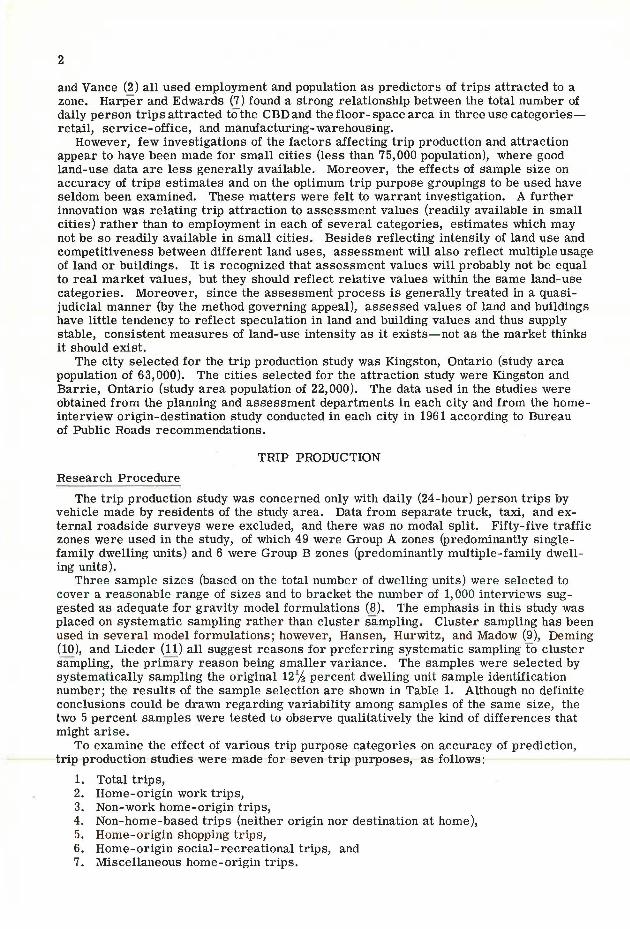
However, few investigations of the factors affecting trip production and attraction appear to have been made for small cities (less than 75,000 population), where good land-use data are less generally available. Moreover, the effects of sample size on accuracy of trips estimates and on the optimum trip purpose groupings to be used have seldom been examined. These matters were felt to warrant investigation. A further innovation was relating trip attraction to assessment values (readily available in small cities) rather than to employment in each of several categories, estimates which may not be so readily available in small cities. Besides reflecting intensity of land use and competitiveness between different land uses, assessment will also reflect multiple usage of land or buildings. It is recognized that assessment values will probably not be equal to real market values, but they should reflect relative values within the same land-use categories. Moreover, since the assessment process is generally treated in a quasi­judicial manner (by the method governing appeal), assessed values of land and buildings have little tendency to reflect speculation in land and building values and thus supply stable, consistent measures of land-use intensity as it exists- not as the market thinks it should exist.

The city selected for the trip production study was Kingston, Ontario (study area population of 63,000). The cities selected for the attraction study were Kingston and Barrie, Ontario (study area population of 22,000). The data used in the studies were obtained from the planning and assessment departments in each city and from the home­interview origin-destination study conducted in each city in 1961 according to Bureau of Public Roads recommendations.

TRIP PRODUCTION

Research Procedure

The trip production study was concerned only with daily (24-hour) person trips by vehicle made by residents of the study area. Data from separate truck, taxi, and ex­ternal roadside surveys were excluded, and there was no modal split. Fifty- five traffic zones were used in the study, of which 49 were Group A zones (predominantly single­family dwelling units) and 6 were Group B zones (predominantly multiple- family dwell­ing units).

Three sample size s (based on the total number of dwelling units) wer e selecte d to cover a r easonable r ange of sizes and to br acket the number of 1, 000 inter views sug­gested as adequate for gravity model formulations (8). The emphasis in this study was placed on systematic sampling r ather than cluste r sa mpling. Cluster sampling has been used in several model formulations; however, Hansen, Hurwitz, and Matlow (9), Deming (10), and Lieder (11) all suggest reasons for preferring systematic sampling to cluster sampling, the primary reason being smaller variance. The samples were selected by systematically sampling the or iginal 121/2 per cent dwelling unit sample identification number; the results of the sample selection are shown in Table 1. Although no definite conclusions could be drawn regarding variability among samples of the same size, the two 5 percent samples were tested to observe qualitatively the kind of differences that might arise.

To examine the effect of various trip purpose categories on accuracy of prediction, trip production studies were made for seven trip purposes, as follows:

1. Total trips, 2. Home-origin work trips, 3. Non-work home-origin trips, 4. Non-home-based trips (neither origin nor destination at home), 5. Home - origin shopping trips, 6. Home-origin social-recreational trips, and 7. Miscellaneous home-origin trips.

3

TABLE 1

KINGSTON SAMPLE SELECTION

Sample Sampling Sample Size: No. of Sample D. U. 1 111 eelected out Designation Rate No. of D. U. 's of every 10 Home-Interview D. U. 1s

S-. 025-K 2. 5% 508

S-.05-1-K s. 0% 983

S-. 05-2-K s. 0% 984

S-, 10-K 10, 0% 1967

Note: "S-. 025-K" designate& a 2f% sample of Kingston data

The category "total trips" for a given zone refers to all person trips by vehicle made by the residents of that zone, regardless of origin or destination of trip, a~d excludes all trips made to or from the zone by non-residents of the zone. The "miscellaneous" category includes trips made for the purposes of personal business, medical-dental service, school, eating a meal, changing mode of travel, and serving passengers.

If it is assumed that all home-origin trips return home, estimates of total trips may be made in three ways, using different combinations of the given trip-purpose cate­gories, as follows:

Total Trip Estimate 1: Trip Purpose Category 1 Total Trip Estimate 2: Trip Purpose Categories 2, 3, 4 Total Trip Estimate 3: Trip Purpose Categories 2, 4, 5, 6, 7

For the sample sizes tested, attempts were made by means of simple and multiple regression analysis to relate sampled trips per D. U. for various purposes to sampled values of the following land-use parameters and characteristics of the zonal population :

X1 Cars/dwelling unit X2 (Car s/dwelling unit)2 = ~ xs Per sons/dwelling unit X4 (Persons/dwelling unit)2 = x2

Xe Airline distance from CBD (tenths of miles) X6 log10 (airline distance from CBD) = log10 Xs x, Residential density (dwelling units/net residential acre) :xs log10 (residential density) = log10 x, X9 Proportion of single-family dwelling units

X10 Percentage of population less than 5 years of age

In the regression analysis, the observations were weighted in accordance with the num­ber of dwelling units in the zone.

The estimation equations of best fit are fully documented (12). The equations for .total trips, home-origin work trips, and home-origin shopping trips are given in Table 2.

The trip estimation equations showed that in Kingston, car ownership was the most reliable single predictor of the trips produced by residents of a zone. For almost all estimates, car ownership was a variable in the estimation equations, and only for home­origin shopping or social-recreational trips was the multiple regression equation an improvement over the simple regression equation using car ownership alone as the in­dependent variable or predictor.

An important observation was that, for a given trip purpose category, although the regression equations derived from the larger sample sizes appear to be better estimat­ing equations by virtue of their larger coefficients of correlation and smaller standard errors, the actual regression equations for different sample sizes show a distinct simi­larity. This similarity was evident for all trip purpose categories except home-origin shopping and social-recreational trips, where greater equation differences occur.

4

Sample

S - • 025 - K

TABLE 2

BEST REGRESSION EQUATIONS FOR TRIP PRODUCTION ESTIMATES (KINGSTON)

Total Tripe

y' = -2. 327 + B. 757x1

r = 0, 87 Se= 1, 39 Trips/D. U ,

Home-Origin Work Tripe

y' = O. 149 + 1, 00Zx1

r = 0,71 Se= 0.29 Trips/D.U,

Home-Origin Shopping Tripe

y' = -0, 017 + 0, 448x6

- 0, 008Sx10

r = 0.47 Se= 0,24 Trips/D.U.

S - , OS .. 1 - K y' = -2. 484 + 8. 289x1 y' = -0. 025 + 1, 09Sx

1 y' = 0, 902 - 1. 152x

1 + 0, 859x

2 - 0.328x

8 r = 0, 90 Se = 1. 05 Trips/ D, U . r::0.75 Se::0,25Trips/D.U , r::0,85 Se::0,12Tripe/D.U.

S-,05-2-K y'= - 2. 710 + 8. 7Slx1 y' = -0. 013 + 1, 14Sx

1 y' = O. 038 + 0, 399x

6 - 0, 01Zx

10 r = 0.91 Se= 1,04 Tripe/D.U. r = O. 79 Se= O. 23 Trips/D, U, r = 0, 66 Se:: O. 14 Tripe/D. U .

.S - • Ul - K y' = -3, 041 + 8, Y83x1 y' = -0. 024 + 1. 124x

1 y' = -0. 056 + 0, 15Sx

2 + O. 209x

6 r = 0, 94 Se= 0, 70 Tripe/D. U , r = O. 81 Se= 0, 19 Trips/D, U . r = 0, 81 Se= O. 10 Trip!!!/D. U ,

Note: y 1 = Trips/D, U .

Trip Estimates and Discussion of Errors

From the regression equations, the number of zonal trips for each trip purpose cate­gory was calculated from the actual zonal values of the basic parameters listed previ­ously and the total number of zonal dwelling units. The actual zonal values of the basic parameters (except for distance from the CBD and residential density, which were mea­sured directly) were obtained from an expansion of the original 121/.i percent sample to 100 percent, due to lack of better data. However, where sample sizes smaller than 121/2 percent were tested, it was assumed that base data comparable to those obtained from the expansion of the 121/.i percent sample to 100 percent would be available from planning sources, and the comparable base data could be substituted in the estimating equations.

For a comparison of actual and estimated trips, the actual number of trips was ob­tained in each case from an expansion of the original 121,h percent home-interview sur­vey data to 100 percent. Although it was recognized that these actual trip values are probably in error, they were used as the standard of comparison in this analysis be­cause they are the generally accepted figures, because they have been used as a stan­dard of comparison in other studies (7, 13, 14), and because there was no available substitute. - - -

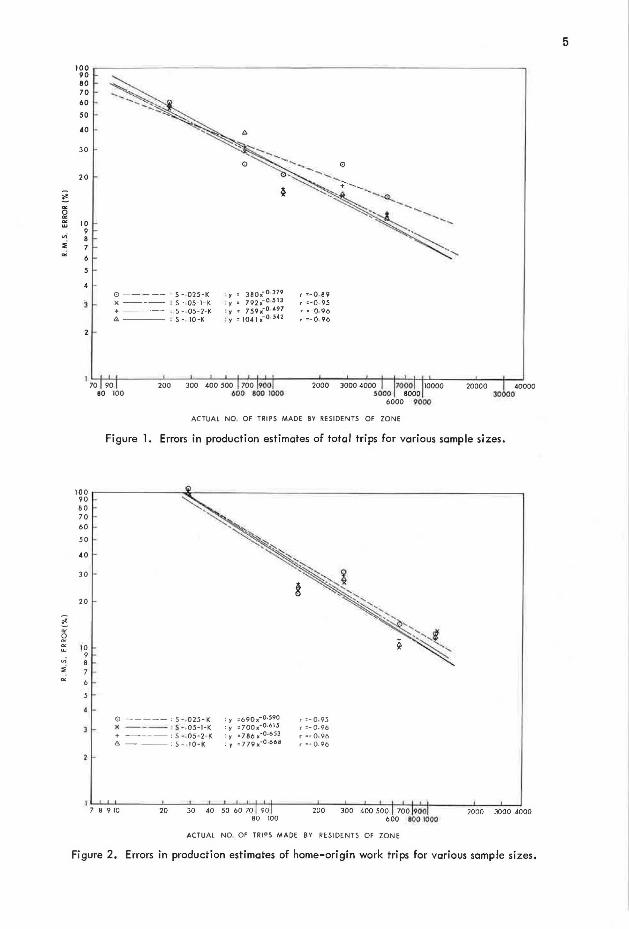
The estimated trip volumes were compared with the corresponding actual trip vol­umes and the errors or discrepancies were calculated. Thest! results are documented elsewhere (12), and are shown graphically for total trips, home-origin work trips, and home-originshopping trips in Figures 1, 2, and 3 respectively.

So that Figures 1-3 could be plotted, actual zonal volumes of trips were grouped into arbitrary ranges of trip volumes. F'or each range of trip volumes, the root-mean­square (RMS) error was calculated and plotted as a percent at the arithmetic mean of the trip volumes in the range:

where

Vest Vact

n

RMS error

estimated volume, corresponding actual volume, and number of zones in range.

Percent RMS error

(vest - V act)2

n

RMS error X 100 v

(1)

(2)

~

; vi i "'

~

~ "' "' i

100 90 80

~ 70 60 ----~:: so 40

30

20

10 9 8 7

6

s

0 ----- s - 02S-K y 3801tO 379 r •-0-B9 )( ----- ' S - · OS-1-K · Y 792.-0 513 r •-Q. 95 + ----- ' s - 05-2-K ' y ' 7 59 .-0. 497 r •-0. 96 8 ' S - . 10-K : y = l041 x- 0 ,5.d2 r •-Q. 96

1 1Lo;-9~0;-----2·00-=---3~0~0-4~o~o~s~o~o-t:1~0~0;9~0·0-t----~2~0~00=--3~0~0~0~4~000'-:-:-r-t7~0~00::-t-r10·00--o---2-o~o-oo---1r--40jooo

100 90 80 70 60

so 4 0

30

20

10 9 -8

BO 100 000 800 1000 5000 8000 30000 6000 9000

ACTUAL NO OF TRIPS MADE BY RESIDENTS OF ZONE

Figure l. Errors in production estimates of total trips for various sample sizes.

0 ----- ' S- .025-K " ---- ' S - .05-1-K + - ---' s -.os-2- K 8 ' S - 10-K

r =-Q. Q5 r =-0. 96 r =-0.96 r =-Q.96

l':-''-"--'----~,.--c'--'---"::---'-:-=:-t-:'-:1'-----:-"-:--~:--:'--L-i--i-:-t--'-t-----"----''---' 7 B 9 10 20 30 40 SO 60 70 90 200 300 400 500 700 900 2000 3000 4000

BO 100 600 800 1000

ACTUAL NO OF TRIPS MADE BY RESIDENTS OF ZONE

Figure 2. Errors in production estimates of home-origin work trips for various sample sizes.

5

6

" ~ w

i cl.

1000 900 -800 700 600

500

400

300

2 0 0

100 90 80 70 60

50

40

30

20

o --- -os- .025-K X---oS--05 -1-K +----oS--05-2-K !!:. oS- . 10-K

., =8 9 4.-0.613 1 • 837x-0 .627 'I = 8 79.:-0·6"2 , = 7 85 )(- 0 .630

r =- 0. 97 r =- Q. 95 r =- 0. 99 r =-Q. 99

l07'-'-8~9~1~0---2~0-~30-~40~5~0-6~0~70-+-9~0+----W~0-~30~0-40~0-5~0-0 ~700~9~0Q-:t----2~0~00-:--~J0~0-0~4000

80 100 0 800 1000

ACTUAL NO OF TRIPS MADE BY RES IDENTS OF ZONE

Figure 3. Errors in prod uct ion est imates of home-origin shopping trips for va rious sample sizes .

where V = mean actual trip volume in range. The percent RMS error was plotted against V.

Now, similar estimating equations, though derived from different sample sizes, would be expected to produce trip estimates of comparable accuracy. Generally this was found to be true, as shown by Figures 1-3. For total trips, home-origin work trips, non-work home-origin trips, non-home-based trips, home-origin social-recrea­tional trips, and miscellaneous home-origin trips, the 5 percent samples appea r to produce results as good as or better than the 10 percent sample, with some overlap of the curves. The 21,4 percent sample is generally slightly poorer than the 5 percent or 10 percent samples, but the differences are not great. For home-origin shopping trips, larger sample sizes appear to improve the estimates slightly, but again the differences are not great. This seems to indicate that sample size (within the range of sample sizes tested) has little effect on accuracy of trip production estimates, and that a con­siderable cost saving could be made by using a relatively small systematic sample. The use of a small sample is, of course, contingent upon the adequacy of a small sample

TABLE 3

COMPARISON OF RMS ERRORS AMONG TffiP PURPOSE CATEGORIES

Trip Purpoe e Cate a o ry Average RMS Error at Zo.W Trip Volume of

10 100 1000 10000 Tat.al

72% Z4% 7% Home-Origin Work Z05o/o 42% 10%

Non-Work Home-Origin 110% 41% 15%

Non-Home- Ba.ee d 69% 24%

Home-Origin Shopping 194% 45%

Home-Ori gin Soc. -Rec . 116% 40%

Miacellaneoua Home -Origin 44% ZO%

7

for trip attraction and distribution as well as for trip production. The effect of sample size on trip attraction estimates is described in a later section of this paper.

In all cases, the percent RMS errors decrease with increasing trip volume. With increased segregation of trip purposes, the trip volumes considered are smaller, and the percent RMS errors are generally larger over the range of trip volumes. However, Table 3 shows that at a given zonal trip volume, the errors are about the same size for all trip purpose categories except for total trips and non-home-based trips, whose er­rors are somewhat larger and approximately equal. Although the percent RMS error at 10 zonal trips shows considerable variability, the absolute difference is quite small and insignificant.

No definite conclusions can be made at present regarding the number of trip purpose categories that should be used in a small city. Table 3 indicates that for a given vol­ume, average percent RMS errors will be approximately equal for all trip purpose cate­gories except total trip and non-home-based trips. It would appear then that the smaller trip purpose categories may be used for production estimates, but the larger trip pur­pose categories should be used as a check on them. Even then, however, the check may not provide much of an improvement over the individual purpose categories used separately. For example, in a given zone assume:

No. of Home-Origin Work Trips No. of Non-Work Home-Origin Trips No. of Non-Home-Based Trips

100 100 30

Assuming that the home-origin trips return home,

No. of Home-Oriented Work Trips No. of Home-Oriented Non-Work Trips No. of Non-Home-Based Trips

Total No. of Zonal Trips

200 200

30

430

Approx. RMS

Error

42% 41%

120%

42% 41%

120%

Approx. Absolute Error

42 41 36

84 82 36

Total Error = 202

Thus using the individual purpose categories, the RMS error"" 202/430 = 47 percent. Using Figure 1, for total trips, at 430 trips, the RMS error is about 37 percent, an improvement of about 10 percent. Using an even further segregation of purpose cate­gories, and assuming the 200 home-oriented non-work trips to be made up of 70 home­oriented shopping trips, 70 home-origin social-recreational trips, and 60 miscellaneous home-oriented trips, the RMS error on total trips is about 62 percent, compared with 47 percent and 37 percent as determined earlier.

Grouping zones into districts also has the general effect of reducing percentage er­rors. When the trip estimates for individual zones were summed to district totals, the percentage errors for the district totals were generally found to be quite small in re­lation to many of the percentage errors in the individual zonal estimates. As with trip purpose categories, as greater definition and segregation are sought (in this case, of land areas), the accuracy of trip production estimates is decreased.

In traffic model analysis, trip production values have generally been assumed cor­rect, and where discrepancies arise in screenline checks or trip length distributions, adjustments have been made to either the attraction figures or the time function used in distribution. This study indicates, however, that errors in trip production estimates may be sizable. Thus, it would seem appropriate to examine the effect that higher pro­duction rates might have on trip distribution and assignment, especially in critical areas.

8

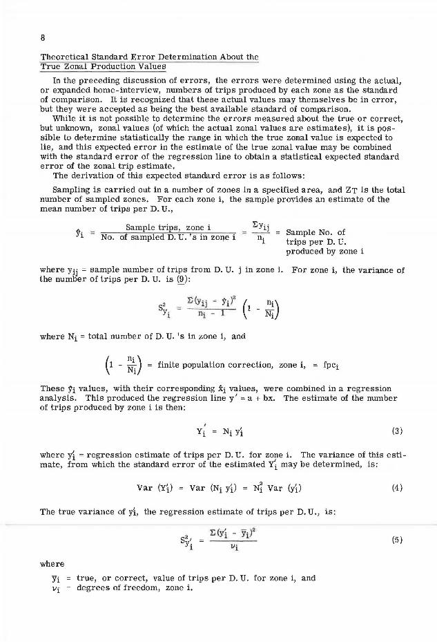
Theoretical Standard Error Determination About the True Zonal Production Values

In the preceding discussion of errors, the errors were determined using the actual, or expanded home-interview, numbers of trips produced by each zone as the standard of comparison. It is recognized that these actual values may themselves be in error, but they were accepted as being the best available standard of comparison.

While it is not possible to determine the errors measured about the true or correct, but unknown, zonal values (of which the actual zonal values are estimates), it is pos­sible to determine statistically the range in which the true zonal value is expected to lie, and this expected error in the estimate of the true zonal value may be combined with the standard error of the regression line to obtain a statistical expected standard error of the zonal trip estimate.

The derivation of this expected standard error is as follows:

Sampling is carried out in a number of zones in a specified area, and ZT is the total number of sampled zones. For each zone i, the sample provides an estimate of the mean number of trips per D. U.,

Sampie trips, zone i ti = No. of sampled D. U. 's in zone i Sample No. of

trips per D. U. produced by zone i

where Yij = sample number of trips from D. U. j in zone i. For zone i, the variance of the numl:ier of trips per D. U. is ~):

where Ni = total number of D. U. 's in zone i, and

( 1 - ~~) = finite population correction, zone i, = fpq

These :9i values, with their corresponding Xi values, were combined in a regression analysis. This produced the regression line y' =a+ bx. The estimate of the number of trips produced by zone i is then:

(3)

where Yi =regression estimate of trips per D. U. for zone i. The variance of this esti­mate, from which the standard error of the estimated Yi may be determined, is:

Var (Yi) = Var (Ni yi) = Ni Var (yj) (4)

The true variance of yi, the regression estimate of trips per D. U., is:

E{yi - Y1>2 (5)

Vi

where

Yi true, or correct, value of trips per D. U. for zone i, and vi degrees of freedom, zone i.

9

This true variance Sy'i is made up of two parts:

1. The variance between the regression estimates and the sample estimates of trips per D. U.-this variance is the square of the standard error of the regression line.

2. The variance between the sample estimates of trips per D. U. and the true values of trips per D. U.-this part is normally not considered, because it is usually assumed that the observed values used in regression analyses are true, not sampled, values.

Considering the sums of squares only,

E [<Yi - Yi) + (Yi - Yi)r E(yi - Yi)2

+ 2!; (yj - :9i) (:9i - Yi) + E (Yi - -Yd

The two parts of the variance are independent. Therefore, the cross-product term be­comes zero, and

(6)

or

i.e.,

(7)

The true value of the zone average, Yi> is unknown. However, in general terminol­ogy, the variance of sample means about the true mean may be determined from

s~ = Sy -= .,;(y - :9)2

(fpc) Y n n(n - 1)

Now, in a given zone i, a sample of ni D. U.' s provides :9i and

S2 _ E(Yij - yif Yi - ni - 1 (fpci)

and the variance of :9i about Yi, the true mean, will be

(8)

and for a given zone,

S2 S2e + ~i Yt = -y (9)

Over all or selected zones, a pooled or weighted estimate of this variance may be determined from

2 2 2 2

v 1 Sy 1

+ v2 Sy2 + Ila Bya + . . . + llp Syp

!Ji + Va + V3 + • · • + Vp

where p represents the p th and final zone to be included in the pooled variance calculation.

10

Now, since in each zone,

2

Sy1· sJi = ni

where SSD = sum of squares of deviations, then,

Therefore :

Also, Vi = ni - 1. Hence,

so that

2

Sy

2 2 2 Since Sy' Se + Sy, therefore

2 2

Sy' = Se +

SS Di (fpq)

ni

Lil + L/2 + ... + Lip

p

'2: (ni - 1) i = 1

p

2: SS Di

i = 1 ni .::

(fpCi)

t ni - p i = 1

p ni (yij - Yi)2

2: L: ni i = 1 j = 1

p

:E ni - p i = 1

SSDp + np- (fpcp)

(1 - ~~)

Two assumptions have been made in the derivation of Eq. 11:

(10)

(11)

1. Within a given zone, the frequency distribution of the number of trips per D. U. is approximately normal; and

2. Among all zones, the variances of the number of trips per D. U., s)r., are ap-proximately equal.

1

Both ammmptions woro found to bo falso. Tho froquoncy distribution in the first as­sumption appear d to be a truncated normal distribution rather than normal, and the Sh varied considerably from zone to zone, often because of an occasional very high

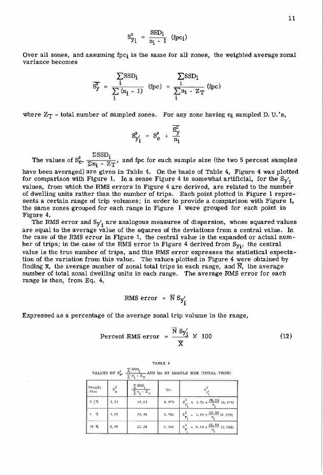
value of trips per D. U. of 20 or more. For this analysis (total trips only), the weighted average zonal variance was deter­

mined for each sample size by summing the individual sums of squares of deviations about the zonal means and dividing by the total number of sampled D. U.'s less the num­ber of zones. Thus, for zone i,

11

SS Di ni - 1 (fpCi)

Over all zones, and assuming fpCi is the same for all zones, the weighted average zonal variance becomes

"82"" y (fpc)

where ZT =total number of sampled zones. For any zone having ni sampled D. U.'s,

s2 S2

1 ::: S2 + _x Yi e ni

ESSDi The values of S~, and fpc for each sample size (the two 5 percent samples

!:ni - ZT ' have been averaged) are given in Table 4. On the basis of Table 4, Figure 4 was plotted for comparison with Figure 1. In a sense Figure 4 is somewhat artificial, for the Sy'i values, from which the RMS errors in Figure 4 are derived, are related to the number of dwelling units rather than the number of trips. Each point plotted in Figure 1 repre­sents a certain range of trip volumes; in order to provide a comparison with Figure 1, the same zones grouped for each range in Figure 1 were grouped for each point in Figure 4.

The RMS error and Sy'i are analogous measures of dispersion, whose squared values are equal to the average value of the squares of the deviations from a central value. In the case of the RMS error in Figure 1, the central value is the expanded or actual num­ber of trips; in the case of the RMS error in Figure 4 derived from SYi• the central value is the true number of trips, and this RMS error expresses the statistical expecta­tion of the variation from this value. The values plotted in Figure 4 were obtained by finding x, the average number of zonal total trips in each range, and N, the average number of total zonal dwelling units in each range. The average RMS error for each range is then, from Eq. 4,

RMS error = N S / Yi

Expressed as a percentage of the average zonal trip volume in the range,

Percent RMS error N Syi x 100

TABLE 4

rsso VALUES OF S~, --1 - AND fpc BY SAMPLE SIZE (TOTAL TRIPS) r 0 1 . ZT

Sample sz rsso, fpc sz

Size • £: 0; - ZT Yi_

2 t% I. 93 28. 05 o. 975 sz = I. 93 .~ (0.975) Yj_ "1

5 % 1. 09 ll. 40 o. 950 sz = I. 09 + ~ (0. 950) Yj_ "1

10 % o. 49 22, 58 o. 900 sz Yi = o. 49 + 1.i . SB (0. 900)

" 1

(12)

12

" ~ "' i

1000 ~~~~~~~~~~~~~~~~~~~~~~~~~~~~~~~~~~ 900 -8 00 -700

600

500

400

300

200

100 90 80 7 0

60

50

40

30

20

-

-

1010 90

80 100

0 - --- 2l ''• ~ --- 51. " --- 10%

Y = 933 .-o.•oo y ; 486 .w:-0.366 y s 359 x-0. 377

r =-0~ 97

r =-0-98 r =-0, 98

200 300 400 500 100 900 2000 JOOO 4000 7000 10000 20000 40000 600 800 1000 5000 8000 30 0

6000 9000

ACTUAL NO OF TRIPS MADE BY RES IDENTS OF ZONE

Figure 4. Relationship between RMS error based on total trips Sy; and trip volume.

Comparison of Figures 1 and 4 indicates that larger errors may be expected statis­tically than are apparently obtained when the actual number of trips is used as the stan­dard of comparison. It is to be expected that some of the actual trip volumes used as standard in Figure 1 are in fact in error, so that the true errors in the trip estimates cannot be determined. On the other hand, if the trip estimation equations are very simi­lar among sample sizes, and if they produce very similar zonal trip volume estimates, it follows that the error curves must be very similar, as they are in Figure 1. Figure 4 therefore shows not the true RMS error, but rather what we might consider the limit of the expected RMS error and the dependence of that limit on sample size.

TRIP ATTRACTION

Research Procedure

The trip attraction study was conducted for both Kingston and Barrie, and it too was concerned only with daily person trips by vehicle made by residents of the study area.

Sa.mple Designation

S-. 04-B

S-. 08-1-B

S-. 08-Z-B

S-. 16-B

S-Total-B

TABLE 5

BARME SAMPLE SELECTION

Sampling .Rate

4.0%

8.03

8. 0%

16. o~.

20 , 03

Sample Size: No. of D. U. 'e

260

504

502

1006

1Z54

No. of Sample D. U. 'e Selected out of every 10 Home-Intervi e w D. U. 1 e

10

13

Fifty zones were used in the Kingston study and 31 zones in the Barrie study. For King­ston, the same sample sizes were used as for the production study: 21,h percent, 5 per­cent, 10 percent, and in addition, the full 121,h percent sample. For Barrie, the sys­tematic sample sizes tested were 4 percent, 8 percent, 16 percent, and the full 20 per­cent sample, with the 16 percent sample size approximating 1, 000 interviews, as shown in Table 5.

The trip purpose categories examined in the attraction study were the same for both Kingston and Barrie, and were designated as follows:

ALL: The total of all purpose categories 1: Trips to work 2: Trips made to conduct personal business 8: Trips made to shop 0: Trips made to home

The modal breakdown was also examined to some extent in that examinations were made for

1. All modes combined (excluding walking trips), and 2. Auto driver and passenger combined.

Since the investigation was based on the assumed existence of a relationship between the trips attracted to an area and certain assessment-area variables, it seemed rea­sonable to assume that if a relationship did exist, it would exist not only for the total trips attracted to any area for various trip purposes but also for different sized samples of these trips. In an attempt to determine a possible relationship, multiple regression analyses were performed on trips obtained from the various samples selected and the following assessment-area variables:

x1 Assessed value of residential land (thousands of dollars) x2 Assessed value of residential buildings (thousands of dollars) X3 Assessed value of commercial land (thousands of dollars) Xi Assessed value of commercial buildings (thousands of dollars) Xs Assessed value of industrial land (thousands of dollars) Xi; Assessed value of industrial buildings (thousands of dollars) x1 Assessed value of public land (thousands of dollars) Xe Assessed value of public buildings (thousands of dollars) Xg Area of residential land (acres)

x10 Area of commercial land (acres) Xu Area of industrial land (acres) X12 Area of public land (acres)

The assessment information was obtained by examining the assessment rolls of each city and recording the assessed value of each piece of land and building under its partic­ular land-use category (residential, commercial, industrial, and public) for the traffic zone in which it was located. The land areas in each land-use category for each traffic zone were obtained by planimetry from the land-use maps prepared by each city.

The estimation equations of best fit are documented in a separate report (12). The equations for all purposes, work trips, and shopping trips, for all modes combined are given in Tables 6 and 7 for Kingston and Barrie respectively.

Again, the equations obtained for each travel mode category and trip purpose ap­peared to be similar in form, for a given city, although there was little or no similarity between cities. This does not necessarily imply that a common relationship is impos­sible. Rather, it is believed that the differences exhibited in this study may reflect variations in assessment philosophies and methods in the two cities.

The relationships developed also appear to be realistic for each city, in that the assessment-area variables tending to have the most pronounced effect in the estimating equations are those which are most logically associated with the trip purpose under consideration; that is, shopping trips are very dependent upon the commercial assess­ment-area variables, work trips are dependent upon commercial, industrial, and pub­lic assessment-area variables, etc.

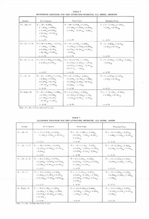
TABLE 6

REGRESSIONS EQUATIONS FOR TRIP ATTRACTION ESTIMATES, ALL MODES, KINGSTON

Sample

B - I 025 - K

S- ~ 05 ,, 1 - K

s - . os ... 2 -- K

S - • 10 - K

S - Tota.I- K

All Purposes

Y' = 163 - 4. 058x1

+ 1, 432x2

- O. 468x3

+ 5. 430x4

+ O. 226x8

+ 23. 64x9

- 19. 37x10

+ 3, 76x11

r = O. 98

Y' = 183 + 0, 900x2

- 0, 91Sx3

+ 4, 236x4

- 1, 78Sx7

+ O. 292x8

+ 10, 57x9

- 26, 04x10

+ 2. 89x11

r = 0, 98

Work Trips

Y 1 = 100 - O. 576x1

+ 1. 352x4

+ 3, 746x5

+ 1. 658x7

+ O. 054x8

+ 4. 89x9

- 13. 4lx10

+ 2. 05x11

r = 0, 97

y1 = -64 - O, 47 lx1

+ O, 838x4

t 1. 767x5

+ 1, 514x7

+ 0, 074x8

+ 4, 17x9

- 12, 30x10

+ 1, 99x11

- 0, 67x12

r = O. 96

Y' = 301+O.944x2

+ 3. 244x4

Y' = -33 + 0, 332x1

+1,27Sx4

+ O. 247x8

+ 2, 7 Sx11

+ l, 350x5

+ O. 30Sx6

+ 1, 07 lx7

+ 0, 099x8

+ 3, OOx9

- 19. 4lx10

+ 0, 73 x11

- 1, Zlx12

r = 0. 96 r = O. 98

y1 = 162 - 3.007x1

+l,115x2

Y 1 = -41- 0.425x1

+ l.03lx4

- O. 503x3

+ 4, 424x4

+ 0, 209x8

+ 20. 47x9

- 24. 16x10

+ 2. 93x11

r = 0, 98

+ 1, 424x5

+ O. l 95x6

+ 1. 250x7

+ O. 092x8

+ 3. 50x9

- 10. 3 lx10

+ 1, 26x 11 - 1. llx 12

t' = 0, 98

Y' = 103 - 2, 850x1

+ 1. 298x2

Y 1 = -2 + 0. 8llx4

+ 0, 439x6

- O. 377x3

+ 4. 186x4

+ 0. 73lx7

+ O. 126x8

+ 1. 19x9

+ O. 189x8 + 17. 23x9

- 21. 96x10

+ 3, 10x11

r = 0, 98

. 5. 8Bx10

+ 0. 70x11

- 2. 37x12

r = O. 98

Note: Y' = No. of trios atha.cted to zone

TABLE 7

Shopping Trips

Y 1 :: 15 - 0, 790x3

+ 1. 6B7x4

- 0.9Bx9

+ 27.09x10

r = 0, 95

Y 1 = 2 - O. 804x3

+ 1, 619x4

- 1. lox9

+ ZS. 9Sx10

r = 0, 93

Y 1 = 4 - O. 142x1

- O. 604x3

+ 1. 514x4

+ 18. 95x10

r = 0, 96

Y' = 9- 0.679x3 + l.519x4

- 1. 06x9

+ 21. 60x10

r = 0, 95

Y' = - 1 - O. 138x1 - O. 702x3

+ 1. 540x4

+ 18, 5Bx10

r = 0, 96

REGRESSION EQUATIONS FOR TRIP ATTRACTION ESTIMATES, ALL MODES, BARRIE

Sa.mple

S - • 04 - B

S - , 08 - 1 - B

S - • 08 - 2 - B

S - • 16 - B

S - Total - B

All Purpoeee

Y' = - 79 + 1. 476xi, + 4. 023x4

- 11, 148x7

+ 9. 9Zx11

+28.99x12

r = O. 92

y1 = - 150 + 4. 719x1

+ O. 617x2

+ 6. 137x3

+ 1. 449x8

+ 17. 76x10

+ 8,33x11

r = O. 96

Y' = - 53 + 1. 34Zx2

+ 5. 75lx3

+ 1, 429x4

- 11. 675x7

+ O. 735x8

+ 9. 2Bx10

+ 8. 4zx11

+ 21, 5Zx12

r = O. 95

Y' = - 139 + 2. 856x1

+ 0, 925x2

+ 2, 06Zx4

+ O. 940x5

+ 0, 724x8

+ 15. 30x 10 + 7, 38x11

+ B. 83xl:i.

r = 0, 97

y1 = _ 96 + 2. 110x1

+ l. 309x2

+ 6. 230x3

+ l, 164x4 - 3. 183x7

+0,939x8

+ ll.4Zx10

+9.45x11

+ 11. 2Zx12

r = 0, 98

Note: Y 1 =No, of trips attracted to zone

Work Trips

Y' = - 16 + O. 849x1

+ 1. 028x4

+ 0. 216x6

- 1, 07x9

+ 4. 20x11

+ l. 14x12

r = O. 97

y1 = - 23 + 1. lllx1

+2.127x3

+ 0, 62Bx4

- 1. 076x5

+ O. 696x6

+ O. 279x8

- 1. 6lx9

+ 2. 28x11

r = 0, 98

Y' = 16 + 3. 3Z6x3

- 0, 325x5

+ 0, 47lx6

- 1. 229x7

+ O. 173x8

+ 1, Z8x11

+ 1, 73x12

r = O. 99

y1 = - 5 + O, 63tx1

+2.475x3

+ O. 34lx4

- O. 654x5

+ 0, 574x6

+ O. 155xi - 1, Oox9

+ 2. 4lx11

+ 1. 49x12

r = O. 99

y1 = - 14 + O. 95lx1

+ 6. 825x3

- O. 738x4 - 1, 616x5 + 1. 063x6

- 1. 06x9

+ 1. 66x12

r = O. 99

Shopping Trips

Y' = - 32 + 1. 054x4 - O. 276x8

+ l. 02x9

+ 4. 90x11

+ 2, 67x12

r = O. 92

Y' = - 57 + 2. 630x3

- O. 100x8

+ 1, 34x9

+ 6. 09x10

- 1. 15x11

r = 0. 91

Y' = - 10 + 2. 16lx3

+ O. 423x5

- O. 047x8

+ O. 45x9

- O. 87x11

r = O. 98

y1 = - 75 + 2. 585x3

+ O. 335x6

- O. 196x8

+ 1. 80x9

+ 7, 15x10

- 3, 90x11

r = O. 91

Y' = - 89 + 3. 046x3

+ O. 370x6

- O. 223x8

+ 2, 2lx9

+ 8, Olx10

- 4. 48x11

r = 0, 90

15

Trip Estimates and Discussion of Errors

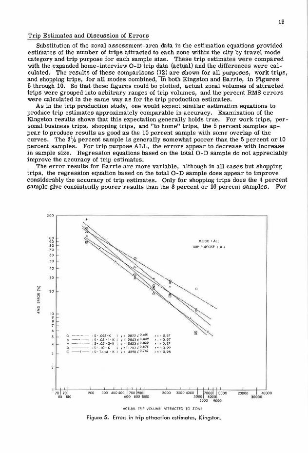
Substitution of the zonal assessment-area data in the estimation equations provided estimates of the number of trips attracted to each zone within the city by travel mode category and trip purpose for each sample size. These trip estimates were compared with the expanded home-interview 0-D trip data (actual) and the differences were cal­culated. The results of these comparisons (12) are shown for all purposes, work trips, and shopping trips, for all modes combined, in both Kingston and Barrie, in Figures 5 through 10. So that these figures could be plotted, actual zonal volumes of attracted trips were grouped into arbitrary ranges of trip volumes, and the percent RMS errors were calculated in the same way as for the trip production estimates.

As in the trip production study, one would expect similar estimation equations to produce trip estimates approximately comparable in accuracy. Examination of the Kingston results shows that this expectation generally holds true. For work trips, per­sonal business trips, shopping trips, and "to home" trips, the 5 percent samples ap­pear to produce results as good as the 10 percent sample with some overlap of the curves. The 21,4 percent sample is generally somewhat poorer than the 5 percent or 10 percent samples. For trip purpose ALL, the errors appear to decrease with increase in sample size. Regression equations based on the total 0-D sample do not appreciably improve the accuracy of trip estimates.

The error results for Barrie are more variable, although in all cases but shopping trips, the regression eq<Uation based on the total 0-D sample does appear to improve considerably the accuracy of trip estimates. Only for shopping trips does the 4 percent sample give consistently poorer results than the 8 percent or 16 percent samples. For

100 90 80 70

60

50

40

30

20

10 9 8

6

4

o ---- s-.025-K : , • 2522,-0.001 x --- S-.05-1-K : y• 284J,-00• 9

+ ---- S- 05-2-K : y•I06JJ,-0, 820 t; --- S-.10-K : y • 11782'-0. 875 0 -T- S- Toto I - K : y = 4898 :a:-0 .762

r • - 0, 97 , .. 0 97 r = - 0.97 r • • 0. 99 r • • 0.98

MODE: All

TRIP PURPOSE : All

0

ACTU.Al TRIP VOLUME ATTRACTED TO ZONE

Figure 5. Errors in trip attraction estimates, Kingston.

20000 40000 30000

16

1000 900 . 800 -700

600

500

400

300

200

10 0 90

!O 80 -

; 70

60 . 50

"' 40 .;

30 . 20

10 9 8

4 •

•ooo

JOOO

1000

1000 •OO 000 700

600

"' JOO

;;

~ 200

IOO

" " 70

"

"

~~ = • ' • 7891

" x + .. "'

----- S·. 025·K ---- s- . OS-1-K ---- S-. OS-2-K ---- S· 10-K --f- S· To1at-K

x

"

: r a 4172 .. - 0·733 : y "' 8299 .-Q.9A3 : r :: 2484 ;ii·O 71A : r = 5114 ,- 0-869 : r "' 6310 it 0- 976

MOOE : ALL

TRIP PURPOSE I !WORK)

r =-0 92 r=-0 96 r =-Q . 93 r=-0 96 r=-0 98

80 100 600 800 1000 ACTUAL TRIP VOLUME ATTRACTED TO ZONE

Figure 6. Errors in trip attraction estimates, Kingston.

MOOE : AU

HllP PUfl:P05E : I I SHOPPING )

0 ---- S - 025-K X --- S • O!H·IC +--- - S-OS·H( 0--- S-10-IC 0-T- S-Tolol - K

,, ·•790 . -o 7to •• -099 1•10167• ' 1l.1 11 r••U.5' l •0.70 1•-0.99 '•3797 , •0.717 •• -098 '•3286 . 0.611 , • -0.99

C S 6 7 8 910 XI JO lkO JOto JQ tO MO JOO .00.JOO 7® t:IO •a IOO tQO IOO ,IOOO

ACTUAt TRIP VOLUME AfC AAC:tru to 10fl [

Figure 7. Errors in trip attraction estimates, Kingston.

4000

--

" ~ ~

::;

~ ~

~ ~

100 90 80 70 60

50

40

30

20

10 9 a 7

• -0---- : s - 0.1 -8 x ---- : s - 08-1-8 + ---- = s - .oe-2-a 1>---:S-16-8 CJ -T--: S -Total B

: y = 376.1:-0. 309 : Y = 789 "-o 517 : Y =513 x-0 • .420 I f o: 542x-0 463 • r =9978.ll'-o~9os

r :-Q. 85 r =-0 91 r =-0 .86 r =-0-83 r =-0 99

MODE: ALL

TRIP PURPOSE : ALL

1 7=0+-=9~0t-----:?~00:--:-30~0,---4~00:-:-50~0:-+~70~0c!:::~---~2~00~0,---~:;;-:~:-+-t;;:!:;:!-ll;;t;:;;;;------;~~-r-;;j 80 JOO 6Q0 B.00 I

ACTUAL TRIP VOLUME ATTRACTED TO ZONE

Figure 8. Errors in trip attraction estimates, Barrie.

300

200

MODE: ALL

TRIP PURPOSE ' 1 {WORK)

100 90 60 70 -60 -

50

40

30

20 0

10 9 6

0----- S- 04- B .. 2461(-0 370 r = - 0 68 x---- 5- 08 - 1- B y• 1705--0. 751 r = - 0. 97 +---- S- ,08-2-B ,. 576 x-0 ,473 r = - 0. 94 ,, ____ s- . 16- e .. 636 )(-0. 586 r = - 0 90 B--r-- S- Total -B .. 2362 IC-0. 941 r = - 0. 97

3 -

2 -

1 ~~~---~-~-~~~~+-'-+---~--~~-~..__ ....... ~..__---~-~~ 7 8 910 20 30 40 50 60 70 90

80 IOI! 200 300 400 500 700 900

oOt'I eoo 1000

ACTUAL TRIP VOLUME ATTRACTED TO ZONE

Figure 9. Errors in trip attraction estimates, Barrie.

2000 3000 4000

17

18

~ ~

i :1

6000 7000 6000 •

5000

4000

3000

2000

1000 900 800 700

600

500

400

300

200

JOO 90 80 70

60

50

40

30 -

20 -

0 -----: S- 04-8 y=l2777 x-1 ,011 x --- : s- 08- 1 - 8 ; y:. 3338 lf0.771 + ----: s- oe- 2 - e ~ y= i101 iro6o9 "' -- S- . 16- B : y = 3624 111·0,793 O -T-: 5-Total - B : y = '1702 11·0,843

r • - o.9s+ f I • Q.97 p - 0.94 ' .. - 0.97 , • - 0.98

MODE: ALL

TRIP PURPOSE' B (SHOPPING)

0

10 ~~~~---'--~-'---'---'---'-...__._LJ ~----'-~--'----'---'---'---'--f-'-j~~~L-----"~..__-'-----ji--1 7 B 9 I 3 4 5 6 7 B 9 10 20 30 40 50 60 70 90 200 300 400 500 700

80 100 600 800

ACTUAL TRIP VOLUME ATTRACTED TO ZONE

Figure 10. Errors in trip attraction estimates, Barrie.

the other four trip purposes, the error curves overlap in such a way that no conclusions can be drawn as to the effect of sample size on estimates of attracted trips.

It may be seen, therefore, that the sample size (within the range of sample sizes tested) has little or no definite and consistent effect on the accuracy of trip attraction estimates. Consequently, it appears that a considerable saving in cost could be achieved by using a relatively small 0-D sample.

For the smaller attracted volumes, it may be noted that the percent RMS error is so great as to cause one to question the value of small trip volumes. This implies that perhaps zone boundary selection should be governed to some extent by the number of trips attracted to the zone.

The attraction study shows that trip attraction estimates, as well as production es­timates, may exhibit sizable errors. Again, however, it is suggested that the estimates are useful, and that it would seem appropriate to examine the effects of higher produc­tion and attraction rates on trip distribution and assignment in critical areas.

Although no calculations were made, the method of determining theoretical standard errors about the true zonal values, as outlined in the production study, should also be applicable, with minor modifications, to trip attraction.

CONCLUSIONS

1. Estimation equations may be developed for small cities which relate trip produc­tion to car ownership primarily as well as to other population and land-use parameters,

19

and which relate trip attraction to assessment and land-use parameters. For trips having the same trip purpose and mode of travel, the equations developed for a given city show similarity and also appear to be logical in that the expected significant variables play a predominant role in the estimating equations.

2. Comparison of the estimating equations for trip attraction for the two cities in­dicates some dissimilarities. It is suggested that variations of this kind might be re­duced if equalization of assessment between cities could be accomplished.

3. The size of the origin-destination sample used to develop the estimating equations does not appear to affect significantly the accuracy of trip estimates, although theoret­ically it would be expected to. (Accuracy here means agreement with expanded 0-D survey results.)

4. The size of the percent RMS error in trip estimation appears to increase with more extensive breakdown or segregation of trip purpose categories and land areas. On the one hand, variation of estimating equations among trip purposes is quite evident (especially for trip attraction), indicating that separate equations would appear to be necessary for estimating these different kinds of trips. On the other hand, it would appear that attempts to stratify trips too extensively will result in rather sizable errors.

REFERENCES

1. Lynch, J. T. Home-Interview Surveys and Related Research Activities. Public Roads, Vol. 30, No. 8, pp. 185-186, June 1959. Also, HRB Bull. 224, pp. 85-88, 1959.

2. Kudlick, W., Fisher, E. S., and Vance, J.A. Intermediate and Final Quality Checks Developing a Traffic Model. Highway Research Record 38, pp. 1-24, 1963.

3. Lynch, J. T., Brokke, G. E., Voorhees, A. M., and Schneider, M. Panel Dis­cussion on Inter-Area Travel Formulas. HRB Bull. 253, pp. 128-138, 1960.

4. Mertz, W. L., and Hamner, L. B. A Study of Factors Related to Urban Travel. Public Roads, Vol. 29, No. 7, pp. 170-174, April 1957.

5. Voorhees, Alan M. A General Theory of Traffic Movement. The 1955 Past Presi­dents' Award Paper, Institute of Traffic Engineers, New Haven, Connecticut.

6. Barnes, Charles F., Jr. Integrating Land Use and Traffic Forecasting. HRB Bull. 297, pp. 1-13, 1961.

7. Harper, B. C. S., and Edwards, H. M. Generation of Person Trips by Areas Within the Central Business District. HRB Bull. 253, pp. 44-61, 1960.

8. Furness, K. P. The Use of a Gravity Model in the Estimation of Traffic. Un­published paper, Traffic Section, Department of Highways, Ontario, Oct. 1961.

9. Hansen, M. H., Hurwitz, W. N., and Madow, W. G. Sample Survey Methods and Theory. Vol. 1, Methods and Applications. John Wiley and Sons, 1953.

10. Deming, W. E. Sampling Techniques. John Wiley and Sons, 1953. 11. Lieder, N. Sampling Techniques Applicable to the Collection of Economic Data.

Public Roads, Vol. 30, No. 11, pp. 246-255, Dec. 1959. 12. Harmelink, M. D., Harper, G. C., and Edwards, H. M. Trip Generation and

Attraction Characteristics in Small Cities. Research Report RR121, Depart­ment of Highways, Ontario, Nov. 1966.

13. Sharpe, G. B., Hansen, W. G., and Hamner, L. B. Factors Affecting Trip Gen­eration of Residential Land-Use Areas. Public Roads, Vol. 30, No. 4, pp. 88-99, Oct. 1958. Also HRB Bull. 203, pp. 20-36, 1958.

14. Wynn, F. H., and Linder, C. E. Tests of Interactance Formulas Derived From 0-D Data. HRB Bull. 253, pp. 62-85, 1960.