Tropical curves and metric graphs - Brown Universitymtchan/thesis_mchan.pdfTropical curves and metric graphs by Melody Tung Chan A dissertation submitted in partial satisfaction of

Tropical curves and metric graphs

by

Melody Tung Chan

A dissertation submitted in partial satisfaction of the

requirements for the degree of

Doctor of Philosophy

in

Mathematics

in the

Graduate Division

of the

University of California, BERKELEY

Committee in charge:

Professor Bernd Sturmfels, ChairProfessor Matthew Baker

Professor Robert LittlejohnProfessor Lauren Williams

Spring 2012


Copyright 2012by

Melody Tung Chan

1

Abstract


by

Melody Tung Chan

Doctor of Philosophy in Mathematics

University of California, BERKELEY

Professor Bernd Sturmfels, Chair

In just ten years, tropical geometry has established itself as an important new fieldbridging algebraic geometry and combinatorics whose techniques have been used to attackproblems in both fields. It also has important connections to areas as diverse as geomet-ric group theory, mirror symmetry, and phylogenetics. Our particular interest here isthe tropical geometry associated to algebraic curves over a field with nonarchimedeanvaluation. This dissertation examines tropical curves from several angles.

An abstract tropical curve is a vertex-weighted metric graph satisfying certain con-ditions (see Definition 2.2.1), while an embedded tropical curve takes the form of a 1-dimensional balanced polyhedral complex in Rn. Both combinatorial objects inform thestudy of algebraic curves over nonarchimedean fields. The connection between the twoperspectives is also very rich and is developed e.g. in [Pay09] and [BPR11]; we give a briefoverview in Chapter 1 as well as a contribution in Chapter 4.

Chapters 2 and 3 are contributions to the study of abstract tropical curves. We beginin Chapter 2 by studying the moduli space of abstract tropical curves of genus g, themoduli space of principally polarized tropical abelian varieties, and the tropical Torellimap, as initiated in [BMV11]. We provide a detailed combinatorial and computationalstudy of these objects and give a new definition of the category of stacky fans, of whichthe aforementioned moduli spaces are objects and the Torelli map is a morphism.

In Chapter 3, we study the locus of tropical hyperelliptic curves inside the modulispace of tropical curves of genus g. Our work ties together two strands in the tropicalgeometry literature, namely the study of the tropical moduli space of curves and tropicalBrill-Noether theory. Our methods are graph-theoretic and extend much of the work ofBaker and Norine [BN09] on harmonic morphisms of graphs to the case of metric graphs.We also provide new computations of tropical hyperelliptic loci in the form of theoremsdescribing their specific combinatorial structure.

Chapter 4 presents joint work with Bernd Sturmfels and is a contribution to thestudy of tropical curves as balanced embedded 1-dimensional polyhedral complexes. Wesay that a plane cubic curve, defined over a field with valuation, is in honeycomb form if itstropicalization exhibits the standard hexagonal cycle shown in Figure 4.1. We explicitlycompute such representations from a given j-invariant with negative valuation, we give

2

an analytic characterization of elliptic curves in honeycomb form, and we offer a detailedanalysis of the tropical group law on such a curve.

Chapter 5 is joint work with Anders Jensen and Elena Rubei and is a departure fromthe subject of tropical curves. In this chapter, we study tropical determinantal varietiesand prevarieties. After recalling the definitions of tropical prevarieties, varieties, andbases, we present a short proof that the 4× 4 minors of a 5× n matrix of indeterminatesform a tropical basis. The methods are combinatorial and involve a study of arrangementsof tropical hyperplanes. Our result together with the results in [DSS05], [Shi10], [Shi11]answer completely the fundamental question of when the r × r minors of a d× n matrixform a tropical basis; see Table 5.1.

i

Contents

List of Figures ii

List of Tables iii

1 Introduction 1

2 Tropical curves, abelian varieties, and the Torelli map 4

2.1 Introduction . . . . . . . . . . . . . . . . . . . . . . . . . . . . . . . . . . 42.2 The moduli space of tropical curves . . . . . . . . . . . . . . . . . . . . . 72.3 Stacky fans . . . . . . . . . . . . . . . . . . . . . . . . . . . . . . . . . . 132.4 Principally polarized tropical abelian varieties . . . . . . . . . . . . . . . 172.5 Regular matroids and the zonotopal subfan . . . . . . . . . . . . . . . . . 272.6 The tropical Torelli map . . . . . . . . . . . . . . . . . . . . . . . . . . . 302.7 Tropical covers via level structure . . . . . . . . . . . . . . . . . . . . . . 33

3 Tropical hyperelliptic curves 38

3.1 Introduction . . . . . . . . . . . . . . . . . . . . . . . . . . . . . . . . . . 383.2 Definitions and notation . . . . . . . . . . . . . . . . . . . . . . . . . . . 403.3 When is a metric graph hyperelliptic? . . . . . . . . . . . . . . . . . . . . 493.4 The hyperelliptic locus in tropical Mg . . . . . . . . . . . . . . . . . . . . 553.5 Berkovich skeletons and tropical plane curves . . . . . . . . . . . . . . . 64

4 Elliptic curves in honeycomb form 68

4.1 Introduction . . . . . . . . . . . . . . . . . . . . . . . . . . . . . . . . . . 684.2 Symmetric cubics . . . . . . . . . . . . . . . . . . . . . . . . . . . . . . . 704.3 Parametrization and implicitization . . . . . . . . . . . . . . . . . . . . . 744.4 The tropical group law . . . . . . . . . . . . . . . . . . . . . . . . . . . . 83

5 Tropical bases and determinantal varieties 90

5.1 Introduction . . . . . . . . . . . . . . . . . . . . . . . . . . . . . . . . . . 905.2 Tropical determinantal varieties . . . . . . . . . . . . . . . . . . . . . . . 925.3 The 4 × 4 minors of a 5 × n matrix are a tropical basis . . . . . . . . . . 95

Bibliography 102

ii

List of Figures

1.1 A tropical plane cubic curve. . . . . . . . . . . . . . . . . . . . . . . . . . 2

2.1 Poset of cells of M tr3 . . . . . . . . . . . . . . . . . . . . . . . . . . . . . 6

2.2 A tropical curve of genus 3 . . . . . . . . . . . . . . . . . . . . . . . . . . 82.3 The stacky fan M tr

2 . . . . . . . . . . . . . . . . . . . . . . . . . . . . . . 102.4 Posets of cells of M tr

2 and M2 . . . . . . . . . . . . . . . . . . . . . . . . 11

2.5 Infinite decomposition of S2≥0 into secondary cones . . . . . . . . . . . . . 19

2.6 Cells of Atr2 . . . . . . . . . . . . . . . . . . . . . . . . . . . . . . . . . . . 21

2.7 The stacky fan Atr2 . . . . . . . . . . . . . . . . . . . . . . . . . . . . . . . 22

2.8 Poset of cells of Atr3 = Acogr

3 . . . . . . . . . . . . . . . . . . . . . . . . . . 32

3.1 A harmonic morphism of degree two . . . . . . . . . . . . . . . . . . . . 403.2 The tropical hyperelliptic curves of genus 3 . . . . . . . . . . . . . . . . . 433.3 The 2-edge-connected tropical hyperelliptic curves of genus 3 . . . . . . . 443.4 Contracting a vertical edge. . . . . . . . . . . . . . . . . . . . . . . . . . 593.5 Contracting two horizontal edges. . . . . . . . . . . . . . . . . . . . . . . 593.6 The ladders of genus 3, 4, and 5. . . . . . . . . . . . . . . . . . . . . . . 603.7 Splitting a vertex v of horizontal multiplicity 2 . . . . . . . . . . . . . . . 623.8 Horizontal splits in G above vertices in T of degrees 1, 2, and 3 . . . . . 633.9 A unimodular triangulation and the tropical plane curve dual to it . . . . 65

4.1 Tropicalizations of plane cubic curves in honeycomb form . . . . . . . . . 694.2 The Berkovich skeleton Σ of an elliptic curve with honeycomb punctures 814.3 A honeycomb cubic and its nine inflection points in groups of three . . . 844.4 The torus in the tropical group law surface . . . . . . . . . . . . . . . . . 864.5 Constraints on the intersection points of a cubic and a line. . . . . . . . . 89

5.1 A hyperplane in TP2 partitions the points of the plane . . . . . . . . . . 96

iii

List of Tables

2.1 Number of maximal cells in the stacky fans M trg , Acogr

g , and Atrg . . . . . . 33

2.2 Total number of cells in the stacky fans M trg , Acogr

g , and Atrg . . . . . . . . 33

5.1 When do the r × r minors of a d× n matrix form a tropical basis? . . . . 92

iv

Acknowledgments

“And remember, also,” added thePrincess of Sweet Rhyme, “that manyplaces you would like to see are just offthe map and many things you want toknow are just out of sight or a littlebeyond your reach. But someday you’llreach them all, for what you learntoday, for no reason at all, will helpyou discover all the wonderful secretsof tomorrow.”

Norton Juster, The Phantom Tollbooth

I am deeply grateful to my advisor, Bernd Sturmfels, for his mentorship and supportthroughout my graduate career. His guidance has shaped me into the mathematician Iam today. I am also indebted to many other mathematicians for patiently teaching meso much, especially Matt Baker, Paul Seymour, and Lauren Williams, as well as fellow orformer Berkeley graduate students Dustin Cartwright, Alex Fink, Felipe Rincon, CynthiaVinzant, and many, many others. My coauthors on the projects appearing in Chapters4 and 5 (Anders Jensen, Elena Rubei, and Bernd Sturmfels) have graciously agreed tohave our joint work appear in my dissertation. The work presented in Chapter 5 grewout of discussions with Spencer Backman and Matt Baker, and I am grateful for theircontributions. I also thank Ryo Masuda for much help with typesetting. I am fortunate tohave been supported by NDSEG and NSF Fellowships during graduate school. Finally, Ithank Amy Katzen for all of her support and patience, and the members of Mrs. Mildred’sBridge Group for providing four years of beautiful music and friendship.

1

Chapter 1

Introduction

In just ten years, tropical geometry has established itself as an important new fieldbridging algebraic geometry and combinatorics whose techniques have been used success-fully to attack problems in both fields. Tropical geometry also has important connectionsto areas as diverse as geometric group theory, mirror symmetry, and phylogenetics.

There are several different ways to describe tropical geometry. On the one hand, it isa “combinatorial shadow” of algebraic geometry [MS10]. Let us start with the followingdefinition. Let K be a field, which we will assume for now to be algebraically closed andcomplete with respect to a nonarchimedean valuation val : K∗ → R on it. Suppose X isan algebraic subvariety of the torus (K∗)n, that is, the solution set to a system of Laurentpolynomials over K. Then the tropicalization of X is the set

Trop(X) = {(val(x1), . . . , val(xn)) ∈ Rn : (x1, . . . , xn) ∈ X}.

(more precisely, it is the closure in Rn, under its usual topology, of this set.) By the the-ory of initial degenerations (see [Stu96], [MS10, Theorem 3.2.4]), these tropical varietiesare made of polyhedral pieces and have many nice combinatorial properties. Further-more, they remember information about classical varieties, for example, their dimensions[BG84]. So, if X was a plane curve, then Trop(X) would be made of 1-dimensional poly-hedra, i.e. line segments and rays, in R2. A tropical plane curve of degree 3 is shownin Figure 1.1; this particular cubic will be revisited in Chapter 4. Note that differentembeddings of a variety X can yield very different tropicalizations.

There is a complementary perspective from which tropical geometry is a tool for takingfinite snapshots of Berkovich analytifications. This perspective has been made explicit inthe paper [BPR11] in the case of curves. Suppose X is a smooth curve over the field K.Then X has a space Xan intrinsically associated to it called its Berkovich analytification[Ber90]. Furthermore, there is a metric on Xan, or more precisely on Xan \ X, andone views the original points of the curve X as infinitely far away. The space Xan is avery useful object to study because it has some key desirable properties that X lacks: itadmits a good notion of an analytic function on it, along the lines of Tate’s pioneeringwork on rigid geometry; but in addition, it has a more desirable topology than X, whichis a totally disconnected space since the nonarchimedean field K itself is. Furthermore,

2

Figure 1.1: A tropical plane cubic curve.

Xan has a canonical deformation retract down to a finite metric graph Γ sitting inside it,called its Berkovich skeleton. There is a canonical choice of such a Γ for curves of genus atleast 2, or for genus 1 curves with a marked point, i.e. elliptic curves. This combinatorialcore Γ, decorated with some nonnegative integer weights, is visible in sufficiently nicetropicalizations (see Theorem 6.20 of [BPR11] for the precise theorem, which is actuallystronger and involves an extended notion of tropicalization inside toric varieties in thesense of [Pay09]). Thus, we call this decorated metric graph Γ an (abstract) tropicalcurve. More precisely:

Definition. An abstract tropical curve is a triple (G,w, ℓ), where G is a connectedmultigraph, ℓ : E(G) → R>0 is a length function on the edges of G, and w : V (G) → Z≥0

is a weight function on the vertices of G such that if w(v) = 0, then v has valence at least3. The genus of the curve is dimH1(G,R) +

∑w(v).

Thus, as suggested above, we have a natural map

trop : Mg,n(K) −→M trg,n

sending a genus g curve over K with n marked points to its skeleton, canonically definedwhen g ≥ 2 or g = n = 1 [BPR11, Remark 5.52].

Abstract tropical curves play a central role in Chapters 2 and 3 of this dissertation.In Chapter 2, we study the moduli space of abstract tropical curves of genus g, themoduli space of principally polarized tropical abelian varieties, and the tropical Torellimap, a study initiated in [BMV11]. In Chapter 3, we study the locus of tropical hy-perelliptic curves inside the moduli space of tropical curves of genus g. We view bothchapters as contributions to understanding the combinatorial side of the study of tropicalcurves, moduli spaces, and Brill-Noether theory. We hope that this work will serve as thecombinatorial underpinning of future developments tightening the relationships betweenrelating algebraic and tropical curves and their moduli, for example by studying the fibersof the map of moduli spaces above.

In Chapter 4, we study elliptic curves in honeycomb form, that is, plane cubic curveswhose tropicalizations are in the combinatorially desirable form shown in Figure 1.1. An

3

elliptic E curve can be put into such a form if and only if the valuation of its j-invariantis negative; equivalently, the abstract tropical curve associated to it consists of a singlevertex plus a loop edge based at that vertex of length − val(j(E)). Put differently, thetropicalization of an elliptic curve in honeycomb form faithfully represents the cycle inEan. Our work can thus be viewed as making more explicit, in the case of elliptic curveswith bad reduction, the abstract tropicalization map trop defined above. It can also beviewed as a computational algebra supplement to [BPR11, §7.1], in which faithful tropi-calizations elliptic curves are considered. In particular, we use explicit computations withboth classical (nonarchimedean) and tropical theta functions to gather specific combina-torial information about elliptic curves and the tropical group law on them, as suggestedby Matt Baker. Chapter 4 is joint work with Bernd Sturmfels.

In Chapter 5, we turn our attention to the study of tropical determinantal varietiesand prevarieties, and we present a short proof that the 4× 4 minors of a 5× n matrix ofindeterminates form a tropical basis. This chapter is joint work with Anders Jensen andElena Rubei.

4

Chapter 2

Tropical curves, abelian varieties,

and the Torelli map

This chapter presents the paper “Combinatorics of the tropical Torelli map” [Cha11a],which will appear in Algebra and Number Theory, with only minor changes.

2.1 Introduction

In this chapter, we undertake a combinatorial and computational study of the tropicalmoduli spaces M tr

g and Atrg and the tropical Torelli map.

There is, of course, a vast literature on the subjects of algebraic curves and modulispaces in algebraic geometry. For example, two well-studied objects are the moduli spaceMg of smooth projective complex curves of genus g and the moduli space Ag of g-dimensional principally polarized complex abelian varieties. The Torelli map

tg : Mg → Ag

then sends a genus g algebraic curve to its Jacobian, which is a certain g-dimensionalcomplex torus. The image of tg is called the Torelli locus or the Schottky locus. Theproblem of how to characterize the Schottky locus inside Ag is already very deep. See,for example, the survey of Grushevsky [Gru09].

The perspective we take here is the perspective of tropical geometry [MS10]. Fromthis viewpoint, one replaces algebraic varieties with piecewise-linear or polyhedral ob-jects. These latter objects are amenable to combinatorial techniques, but they still carryinformation about the former ones. Roughly speaking, the information they carry hasto do with what is happening “at the boundary” or “at the missing points” of the alge-braic object.

For example, the tropical analogue of Mg, denotedM trg , parametrizes certain weighted

metric graphs, and it has a poset of cells corresponding to the boundary strata of theDeligne-Mumford compactification Mg of Mg. Under this correspondence, a stable curveC in Mg is sent to its so-called dual graph. The irreducible components of C, weighted

5

by their geometric genus, are the vertices of this graph, and each node in the intersectionof two components is recorded with an edge. The correspondence in genus 2 is shown inFigure 2.4. A rigorous proof of this correspondence was given by Caporaso in [Cap10,Section 5.3].

We remark that the correspondence above yields dual graphs that are just graphs,not metric graphs. One can refine the correspondence using Berkovich analytifications,whereby an algebraic curve over a complete nonarchimedean valued field is associatedto its Berkovich skeleton, which is intrinsically a metric graph. In this way, one obtainsa map between classical and tropical moduli spaces. This very interesting perspective,developed in [BPR11, Section 5], was already mentioned in Chapter 1, and additionallyplays a crucial role in Chapter 4, a study of tropical elliptic curves in honeycomb form.

The starting point of this chapter is the recent paper by Brannetti, Melo, and Viviani[BMV11]. In that paper, the authors rigorously define a plausible category for tropi-cal moduli spaces called stacky fans. (The term “stacky fan” is due to the authors of[BMV11], and is unrelated to the construction of Borisov, Chen, and Smith in [BCS05]).They further define the tropical versions M tr

g and Atrg of Mg and Ag and a tropical Torelli

map between them, and prove many results about these objects, some of which we willreview here.

Preceding that paper is the foundational work of Mikhalkin in [Mik06b] and of Mikhal-kin and Zharkov [MZ07], in which tropical curves and Jacobians were first introduced andstudied in detail. The notion of tropical curves in [BMV11] is slightly different from theoriginal definition, in that curves now come equipped with vertex weights. We should alsomention the work of Caporaso [Cap10], who proves geometric results on M tr

g consideredjust as a topological space, and Caporaso and Viviani [CV10], who prove a tropicalTorelli theorem stating that the tropical Torelli map is “mostly” injective, as originallyconjectured in [MZ07].

In laying the groundwork for the results we will present here, we ran into some incon-sistencies in [BMV11]. It seems that the definition of a stacky fan there is inadvertentlyrestrictive. In fact, it excludes M tr

g and Atrg themselves from being stacky fans. Also,

there is a topological subtlety in defining Atrg , which we will address in §4.4. Thus, we

find ourself doing some foundational work here too.We begin in Section 2 by recalling the definition in [BMV11] of the tropical moduli

space M trg and presenting computations, summarized in Theorem 2.2.12, for g ≤ 5. With

M trg as a motivating example, we attempt a better definition of stacky fans in Section

3. In Section 4, we define the space Atrg , recalling the beautiful combinatorics of Voronoi

decompositions along the way, and prove that it is Hausdorff. Note that our definitionof this space, Definition 2.4.10, is different from the one in [BMV11, Section 4.2], and itcorrects a minor error there. In Section 5, we study the combinatorics of the zonotopalsubfan. We review the tropical Torelli map in Section 6; Theorem 2.6.4 presents com-putations on the tropical Schottky locus for g ≤ 5. Tables 1 and 2 compare the numberof cells in the stacky fans M tr

g , the Schottky locus, and Atrg for g ≤ 5. In Section 7, we

partially answer a question suggested by Diane Maclagan: we give finite-index covers ofAtr

2 and Atr3 that satisfy a tropical-type balancing condition.

6

00

00

0

00

0 0

0 0

0

00

00 0 0

0 0 0 00 0 00

0 1

0 0 0 0

1 0 0 0 0 0 0

0 00

0

100

0

00 00

1

0000 1 0 0 00 0 0 1 00 1 1 0 0 1 0 0 1 0 1 0

101

0

0 10 10 10 1 0 1 01 1 1 01 0 1

10

1

1

1 11 20 11 1 1 1

2 21

3

Figure 2.1: Poset of cells of M tr3 , color-coded according to their images in Atr

3 via thetropical Torelli map.

7

2.2 The moduli space of tropical curves

In this section, we review the construction in [BMV11] of the moduli space of tropicalcurves of a fixed genus g (see also [Mik06b]). This space is denoted M tr

g . Then, we presentexplicit computations of these spaces in genus up to 5.

We will see that the moduli space M trg is not itself a tropical variety, in that it does not

have the structure of a balanced polyhedral fan ([MS10, Definition 3.3.1]). That wouldbe too much to expect, as it has automorphisms built into its structure that preciselygive rise to “stackiness.” Contrast this with the situation of moduli space M0,n of tropicalrational curves with n marked points, constructed and studied in [GKM09], [Mik06a], and[SS04]. As expected by analogy with the classical situation, this latter space is well knownto have the structure of a tropical variety that comes from the tropical GrassmannianGr(2, n).

§2.2.1 Definition of tropical curves.

Before constructing the moduli space of tropical curves, let us review the definition of atropical curve.

First, recall that a metric graph is a pair (G, l), where G is a finite connected graph,loops and parallel edges allowed, and l is a function

l : E(G) → R>0

on the edges of G. We view l as recording lengths of the edges of G. The genus of agraph G is the rank of its first homology group:

g(G) = |E| − |V | + 1.

Definition 2.2.1. A tropical curve C is a triple (G, l, w), where (G, l) is a metric graph(so G is connected), and w is a weight function

w : V (G) → Z≥0

on the vertices of G, with the property that every weight zero vertex has degree at least3.

Definition 2.2.2. Two tropical curves (G, l, w) and (G′, l′, w′) are isomorphic if there

is an isomorphism of graphs G∼=−→ G′ that preserves edge lengths and preserves vertex

weights.

We are interested in tropical curves only up to isomorphism. When we speak of atropical curve, we will really mean its isomorphism class.

Definition 2.2.3. Given a tropical curve C = (G, l, w), write

|w| :=∑

v∈V (G)

w(v).

8

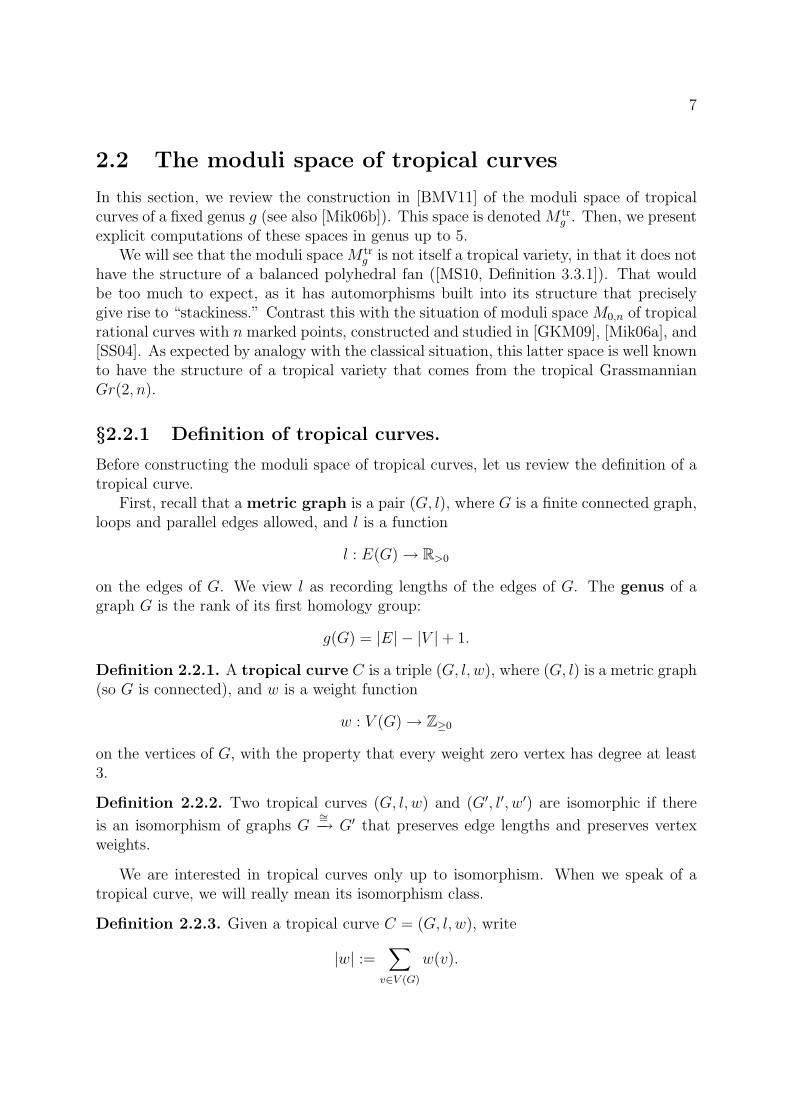
ac

b 01

Figure 2.2: A tropical curve of genus 3. Here, a, b, c are fixed positive real numbers.

Then the genus of C is defined to be

g(C) = g(G) + |w|.

In this chapter, we will restrict our attention to tropical curves of genus at least 2.The combinatorial type of C is the pair (G,w), in other words, all of the data of

C except for the edge lengths.

Remark 2.2.4. Informally, we view a weight of k at a vertex v as k loops, based at v,of infinitesimally small length. Each infinitesimal loop contributes once to the genus ofC. Furthermore, the property that only vertices with positive weight may have degree 1or 2 amounts to requiring that, were the infinitesimal loops really to exist, every vertexwould have degree at least 3.

Permitting vertex weights will ensure that the moduli spaceM trg , once it is constructed,

is complete. That is, a sequence of genus g tropical curves obtained by sending the lengthof a loop to zero will still converge to a genus g curve. Furthermore, permitting vertexweights allows the combinatorial types of genus g tropical curves to correspond preciselyto dual graphs of stable curves in Mg, as discussed in the introduction and in [Cap10,Section 5.3]. See Figure 2.4.

Figure 2.2 shows an example of a tropical curve C of genus 3. Note that if we allowthe edge lengths l to vary over all positive real numbers, we obtain all tropical curves ofthe same combinatorial type as C. This motivates our construction of the moduli spaceof tropical curves below. We will first group together curves of the same combinatorialtype, obtaining one cell for each combinatorial type. Then, we will glue our cells togetherto obtain the moduli space.

§2.2.2 Definition of the moduli space of tropical curves

Fix g ≥ 2. Our goal now is to construct a moduli space for genus g tropical curves, thatis, a space whose points correspond to tropical curves of genus g and whose geometryreflects the geometry of the tropical curves in a sensible way. The following constructionis due to the authors of [BMV11].

First, fix a combinatorial type (G,w) of genus g. What is a parameter space for all

tropical curves of this type? Our first guess might be a positive orthant R|E(G)|>0 , that is,

a choice of positive length for each edge of G. But we have overcounted by symmetries

9

of the combinatorial type (G,w). For example, in Figure 2.2, (a, b, c) = (1, 2, 3) and(a, b, c) = (1, 3, 2) give the same tropical curve.

Furthermore, with foresight, we will allow lengths of zero on our edges as well, withthe understanding that a curve with some zero-length edges will soon be identified withthe curve obtained by contracting those edges. This suggests the following definition.

Definition 2.2.5. Given a combinatorial type (G,w), let the automorphism group

Aut(G,w) be the set of all permutations ϕ : E(G) → E(G) that arise from weight-preserving automorphisms ofG. That is, Aut(G,w) is the set of permutations ϕ : E(G) →E(G) that admit a permutation π : V (G) → V (G) which preserves the weight functionw, and such that if an edge e ∈ E(G) has endpoints v and w, then ϕ(e) has endpointsπ(v) and π(w).

Now, the group Aut(G,w) acts naturally on the set E(G), and hence on the orthant

RE(G)≥0 , with the latter action given by permuting coordinates. We define C(G,w) to be

the topological quotient space

C(G,w) =RE(G)

≥0

Aut(G,w).

Next, we define an equivalence relation on the points in the union∐

C(G,w),

as (G,w) ranges over all combinatorial types of genus g. Regard a point x ∈ C(G,w)as an assignment of lengths to the edges of G. Now, given two points x ∈ C(G,w) andx′ ∈ C(G′, w′), let x ∼ x′ if the two tropical curves obtained from them by contracting alledges of length zero are isomorphic. Note that contracting a loop, say at vertex v, meansdeleting that loop and adding 1 to the weight of v. Contracting a nonloop edge, say withendpoints v1 and v2, means deleting that edge and identifying v1 and v2 to obtain a newvertex whose weight is w(v1) + w(v2).

Now we glue the cells C(G,w) along ∼ to obtain our moduli space:

Definition 2.2.6. The moduli space M trg is the topological space

M trg :=

∐C(G,w)/∼,

where the disjoint union ranges over all combinatorial types of genus g, and ∼ is theequivalence relation defined above.

In fact, the space M trg carries additional structure: it is an example of a stacky fan.

We will define the category of stacky fans in Section 3.

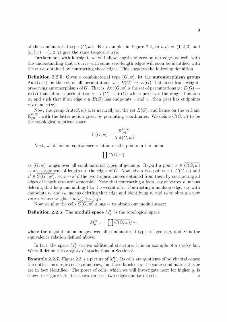
Example 2.2.7. Figure 2.3 is a picture of M tr2 . Its cells are quotients of polyhedral cones;

the dotted lines represent symmetries, and faces labeled by the same combinatorial typeare in fact identified. The poset of cells, which we will investigate next for higher g, isshown in Figure 2.4. It has two vertices, two edges and two 2-cells. ⋄

10

00 00

0

0

0

10

10

1

1

1

11

2

Figure 2.3: The stacky fan M tr2 .

Remark 2.2.8. One can also construct the moduli space of genus g tropical curves withn marked points using the same methods, as done for example in the recent survey ofCaporaso [Cap11a].

§2.2.3 Explicit computations of M tr

g

Our next goal will be to compute the space M trg for g at most 5. The computations were

done in Mathematica.What we compute, to be precise, is the partially ordered set Pg on the cells of M tr

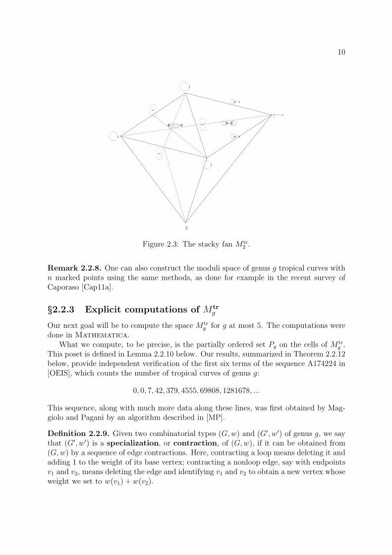
g .This poset is defined in Lemma 2.2.10 below. Our results, summarized in Theorem 2.2.12below, provide independent verification of the first six terms of the sequence A174224 in[OEIS], which counts the number of tropical curves of genus g:

0, 0, 7, 42, 379, 4555, 69808, 1281678, ...

This sequence, along with much more data along these lines, was first obtained by Mag-giolo and Pagani by an algorithm described in [MP].

Definition 2.2.9. Given two combinatorial types (G,w) and (G′, w′) of genus g, we saythat (G′, w′) is a specialization, or contraction, of (G,w), if it can be obtained from(G,w) by a sequence of edge contractions. Here, contracting a loop means deleting it andadding 1 to the weight of its base vertex; contracting a nonloop edge, say with endpointsv1 and v2, means deleting the edge and identifying v1 and v2 to obtain a new vertex whoseweight we set to w(v1) + w(v2).

11

00

0

00

10

1 11

2

Figure 2.4: Posets of cells of M tr2 (left) and of M2 (right).

Lemma 2.2.10. The relation of specialization on genus g combinatorial types yields agraded partially ordered set Pg on the cells of M tr

g . The rank of a combinatorial type(G,w) is |E(G)|.

Proof. It is clear that we obtain a poset; furthermore, (G′, w′) is covered by (G,w) pre-cisely if (G′, w′) is obtained from (G,w) by contracting a single edge. The formula forthe rank then follows.

For example, P2 is shown in Figure 2.4; it also appeared in [BMV11, Figure 1]. Theposet P3 is shown in Figure 2.1. It is color-coded according to the Torelli map, as explainedin Section 6.

Our goal is to compute Pg. We do so by first listing its maximal elements, and thencomputing all possible specializations of those combinatorial types. For the first step,we use Proposition 3.2.4(i) in [BMV11], which characterizes the maximal cells of M tr

g :

they correspond precisely to combinatorial types (G, 0), where G is a connected 3-regulargraph of genus g, and 0 is the zero weight function on V (G). Connected, 3-regular graphsof genus g are equivalently characterized as connected, 3-regular graphs on 2g−2 vertices.These have been enumerated:

Proposition 2.2.11. The number of maximal cells of M trg is equal to the (g − 1)st term

in the sequence

2, 5, 17, 71, 388, 2592, 21096, 204638, 2317172, 30024276, 437469859, . . .

Proof. This is sequence A005967 in [OEIS], whose gth term is the number of connected3-regular graphs on 2g vertices.

12

In fact, the connected, 3-regular graphs of genus g have been conveniently writtendown for g at most 6. This work was done in the 1970s by Balaban, a chemist whoseinterests along these lines were in molecular applications of graph theory. The graphs forg ≤ 5 appear in his article [Bal76], and the 388 genus 6 graphs appear in [Bal70].

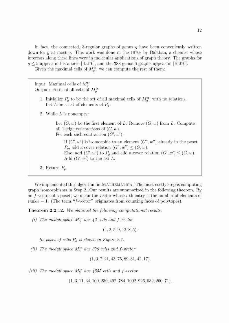
Given the maximal cells of M trg , we can compute the rest of them:

Input: Maximal cells of M trg

Output: Poset of all cells of M trg

1. Initialize Pg to be the set of all maximal cells of M trg , with no relations.

Let L be a list of elements of Pg.

2. While L is nonempty:

Let (G,w) be the first element of L. Remove (G,w) from L. Computeall 1-edge contractions of (G,w).For each such contraction (G′, w′):

If (G′, w′) is isomorphic to an element (G′′, w′′) already in the posetPg, add a cover relation (G′′, w′′) ≤ (G,w).Else, add (G′, w′) to Pg and add a cover relation (G′, w′) ≤ (G,w).Add (G′, w′) to the list L.

3. Return Pg.

We implemented this algorithm in Mathematica. The most costly step is computinggraph isomorphisms in Step 2. Our results are summarized in the following theorem. Byan f -vector of a poset, we mean the vector whose i-th entry is the number of elements ofrank i− 1. (The term “f -vector” originates from counting faces of polytopes).

Theorem 2.2.12. We obtained the following computational results:

(i) The moduli space M tr3 has 42 cells and f -vector

(1, 2, 5, 9, 12, 8, 5).

Its poset of cells P3 is shown in Figure 2.1.

(ii) The moduli space M tr4 has 379 cells and f -vector

(1, 3, 7, 21, 43, 75, 89, 81, 42, 17).

(iii) The moduli space M tr5 has 4555 cells and f -vector

(1, 3, 11, 34, 100, 239, 492, 784, 1002, 926, 632, 260, 71).

13

Remark 2.2.13. The data of P3, illustrated in Figure 2.1, is related, but not identical,to the data obtained by T. Brady in [Bra93, Appendix A]. In that paper, the authorenumerates the cells of a certain deformation retract, called K3, of Culler-VogtmannOuter Space [CV84], modulo the action of the group Out(F3). In that setting, one onlyneeds to consider bridgeless graphs with all vertices of weight 0, thus throwing out allbut 8 cells of the poset P3. In turn, the cells of K3/Out(Fn) correspond to chains in theposet on those eight cells. It is these chains that are listed in Appendix A of [Bra93].

Note that the pure part of M tr′

g , that is, those tropical curves in M tr′

g with all vertexweights zero, is a quotient of rank g Outer Space by the action of the outer automorphismgroup Out(Fg). We believe that further exploration of the connection between OuterSpace andM tr

g would be interesting to researchers in both tropical geometry and geometricgroup theory.

Remark 2.2.14. What is the topology of M trg ? Of course, M tr

g is always contractible:there is a deformation retract onto the unique 0-dimensional cell. So to make this questioninteresting, we restrict our attention to the subspace M tr′

g of M trg consisting of graphs with

total edge length 1, say. For example, by looking at Figure 2.3, we can see that M tr′

2 isstill contractible. We would like to know if the space M tr′

g is also contractible for larger g.

2.3 Stacky fans

In Section 2, we defined the space M trg . In Sections 4 and 6, we will define the space

Atrg and the Torelli map ttrg : M tr

g → Atrg . For now, however, let us pause and define the

category of stacky fans, of which M trg and Atr

g are objects and ttrg is a morphism. Thereader is invited to keep M tr

g in mind as a running example of a stacky fan.The purpose of this section is to offer a new definition of stacky fan, Definition 2.3.2,

which we hope fixes an inconsistency in the definition by Brannetti, Melo, and Viviani,Definition 2.1.1 of [BMV11]. We believe that their condition for integral-linear gluingmaps is too restrictive and fails for M tr

g and Atrg . See Remark 2.3.6. However, we do

think that their definition of a stacky fan morphism is correct, so we repeat it in Definition2.3.5. We also prove that M tr

g is a stacky fan according to our new definition. The prooffor Atr

g is deferred to §4.3.

Definition 2.3.1. A rational open polyhedral cone in Rn is a subset of Rn of theform {a1x1+ · · ·+atxt : ai ∈ R>0}, for some fixed vectors x1, . . . , xt ∈ Zn. By convention,we also allow the trivial cone {0}.

Definition 2.3.2. Let X1 ⊆ Rm1 , . . . , Xk ⊆ Rmk be full-dimensional rational open poly-hedral cones. For each i = 1, . . . , k, let Gi be a subgroup of GLmi

(Z) which fixes the coneXi setwise, and let Xi/Gi denote the topological quotient thus obtained. The action ofGi on Xi extends naturally to an action of Gi on the Euclidean closure Xi, and we letXi/Gi denote the quotient.

14

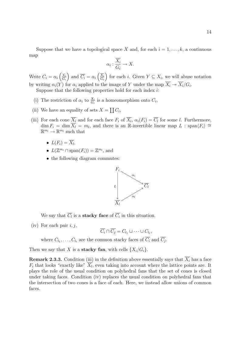
Suppose that we have a topological space X and, for each i = 1, . . . , k, a continuousmap

αi :Xi

Gi

→ X.

Write Ci = αi

(Xi

Gi

)and Ci = αi

(Xi

Gi

)for each i. Given Y ⊆ Xi, we will abuse notation

by writing αi(Y ) for αi applied to the image of Y under the map Xi ։ Xi/Gi.Suppose that the following properties hold for each index i:

(i) The restriction of αi to Xi

Giis a homeomorphism onto Ci,

(ii) We have an equality of sets X =∐Ci,

(iii) For each cone Xi and for each face Fi of Xi, αi(Fi) = Cl for some l. Furthermore,dimFi = dimXl = ml, and there is an R-invertible linear map L : span〈Fi〉 ∼=Rml → Rml such that

• L(Fi) = Xl,

• L(Zmi ∩ span(Fi)) = Zml , and

• the following diagram commutes:

Fi

L

��

αi

&&MMMMMMMMMMMMM

Cl

Xl

αl

88rrrrrrrrrrrrr

We say that Cl is a stacky face of Ci in this situation.

(iv) For each pair i, j,Ci ∩ Cj = Cl1 ∪ · · · ∪ Clt ,

where Cl1 , . . . , Clt are the common stacky faces of Ci and Cj.

Then we say that X is a stacky fan, with cells {Xi/Gi}.

Remark 2.3.3. Condition (iii) in the definition above essentially says that Xi has a faceFi that looks “exactly like” Xl, even taking into account where the lattice points are. Itplays the role of the usual condition on polyhedral fans that the set of cones is closedunder taking faces. Condition (iv) replaces the usual condition on polyhedral fans thatthe intersection of two cones is a face of each. Here, we instead allow unions of commonfaces.

15

Theorem 2.3.4. The moduli space M trg is a stacky fan with cells

C(G,w) =RE(G)>0

Aut(G,w)

as (G,w) ranges over genus g combinatorial types. Its points are in bijection with tropicalcurves of genus g.

Proof. Recall that

M trg =

∐C(G,w)

∼,

where ∼ is the relation generated by contracting zero-length edges. Thus, each equivalenceclass has a unique representative (G0, w, l) corresponding to an honest metric graph: onewith all edge lengths positive. This gives the desired bijection.

Now we prove that M trg is a stacky fan. For each (G,w), let

αG,w : C(G,w) →

∐C(G′, w′)

∼

be the natural map. Now we check each of the requirements to be a stacky fan, in theorder (ii), (iii), (iv), (i).

For (ii), the fact that

M trg =

∐C(G,w)

follows immediately from the observation above.Let us prove (iii). Given a combinatorial type (G,w), the corresponding closed cone is

RE(G)≥0 . A face F of RE(G)

≥0 corresponds to setting edge lengths of some subset S of the edgesto zero. Let (G′, w′) be the resulting combinatorial type, and let π : E(G)\S → E(G′) bethe natural bijection (it is well-defined up to (G′, w′)-automorphisms, but this is enough).Then π induces an invertible linear map

Lπ : RE(G)\S −→ RE(G′)

with the desired properties. Note also that the stacky faces of C(G,w) are thus all possiblespecializations C(G′, w′).

For (iv), given two combinatorial types (G,w) and (G′, w′), then

C(G,w) ∩ C(G′, w′)

consists of the union of all cells corresponding to common specializations of (G,w) and(G′, w′). As noted above, these are precisely the common stacky faces of C(G,w) andC(G′, w′).

For (i), we show that αG,w restricted to C(G,w) = RE(G)>0 /Aut(G,w) is a homeomor-

phism onto its image. It is continuous by definition of αG,w and injective by definition of

∼. Let V be closed in C(G,w), say V = W ∩C(G,w) where W is closed in C(G,w). To

16

show that αG,w(V ) is closed in αG,w(C(G,w)), it suffices to show that αG,w(W ) is closedin M tr

g . Indeed, the fact that the cells C(G,w) are pairwise disjoint in M trg implies that

αG,w(V ) = αG,w(W ) ∩ αG,w(C(G,w)).

Now, note that M trg can equivalently be given as the quotient of the space

∐

(G,w)

RE(G)≥0

by all possible linear maps Lπ arising as in the proof of (iii). All of the maps Lπ identify

faces of cones with other cones. Now let W denote the lift of W to RE(G)≥0 ; then for

any other type (G′, w′), we see that the set of points in RE(G′)≥0 that are identified with

some point in W is both closed and Aut(G′, w′)-invariant, and passing to the quotient

RE(G′)≥0 /Aut(G′, w′) gives the claim.

We close this section with the definition of a morphism of stacky fans. The tropicalTorelli map, which we will define in Section 6, will be an example.

Definition 2.3.5. [BMV11, Definition 2.1.2] Let

X1 ⊆ Rm1 , . . . , Xk ⊆ Rmk , Y1 ⊆ Rn1 , . . . , Yl ⊆ Rnl

be full-dimensional rational open polyhedral cones. Let G1 ⊆ GLm1(Z), . . . , Gk ⊆GLmk

(Z), H1 ⊆ GLn1(Z), . . . , Hl ⊆ GLnl(Z) be groups stabilizing X1, . . . , Xk, Y1, . . . , Yl

respectively. Let X and Y be stacky fans with cells

{Xi

Gi

}k

i=1

,

{YjHj

}l

j=1

,

Denote by αi and βj the maps Xi

Gi→ X and

Yj

Hj→ Y that are part of the stacky fan data

of X and Y .Then a morphism of stacky fans from X to Y is a continuous map π : X → Y

such that for each cell Xi/Gi there exists a cell Yj/Hj such that

(i) π(αi

(Xi

Gi

))⊆ βj

(Yj

Hj

), and

(ii) there exists an integral-linear map

L : Rmi → Rnj ,

that is, a linear map defined by a matrix with integer entries, restricting to a map

L : Xi → Yj,

17

such that the diagram below commutes:

Xi//

L

��

αi(Xi/Gi)

π

��

Yj // βj(Yj/Hj)

Remark 2.3.6. Here is why we believe the original definition of a stacky fan, Definition2.1.1 of [BMV11], is too restrictive. The original definition requires that for every pair ofcones Xi and Xj, there exists a linear map L : Xi → Xj that induces the inclusion

αi

(Xi

Gi

)∩ αj

(Xj

Gj

)→ αj

(Xj

Gj

).

We claim that such a map does not always exist in the cases of M trg and Atr

g . For example,

let Xi be the maximal cone of M tr2 drawn on the left in Figure 2.3, and let Xj be the

maximal cone drawn on the right. There is no map from Xi to Xj that takes each of thethree facets of Xi isomorphically to a single facet of Xj, as would be required. There isa similar problem for Atr

g .

2.4 Principally polarized tropical abelian varieties

The purpose of this section is to construct the moduli space of principally polarizedtropical abelian varieties, denoted Atr

g . Our construction is different from the one in[BMV11], though it is still very much inspired by the ideas in that paper. The reasonfor presenting a new construction here is that a topological subtlety in the constructionthere prevents their space from being a stacky fan as claimed in [BMV11, Thm. 4.2.4].

We begin in §4.1 by recalling the definition of a principally polarized tropical abelianvariety. In §4.2, we review the theory of Delone subdivisions and the main theorem ofVoronoi reduction theory. We construct Atr

g in §4.3 and prove that it is a stacky fan andthat it is Hausdorff. We remark on the difference between our construction and the onein [BMV11] in §4.4.

§2.4.1 Definition of principally polarized tropical abelian vari-

ety

Fix g ≥ 1. Following [BMV11] and [MZ07], we define a principally polarized tropical

abelian variety, or pptav for short, to be a pair

(Rg/Λ, Q),

where Λ is a lattice of rank g in Rg (i.e. a discrete subgroup of Rg that is isomorphicto Zg), and Q is a positive semidefinite quadratic form on Rg whose nullspace is rational

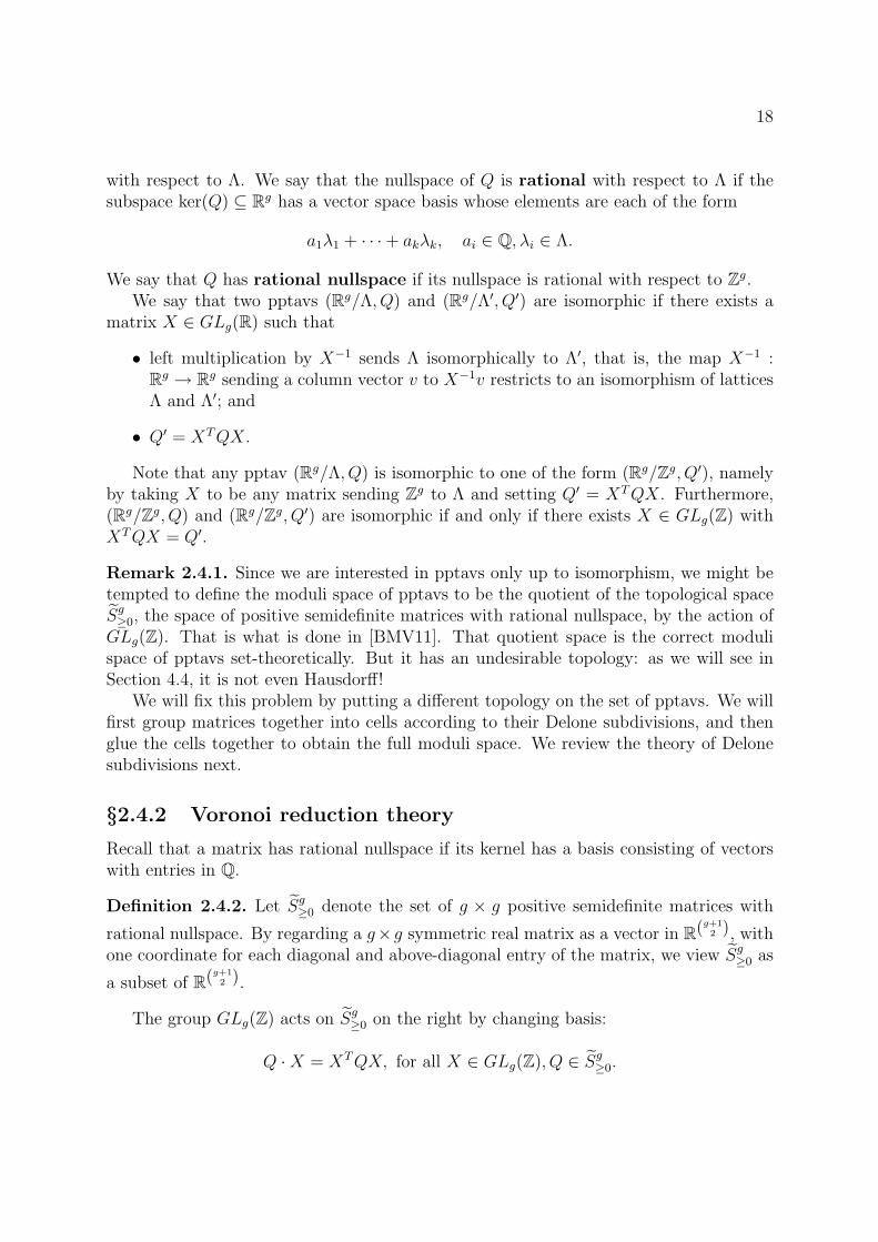
18

with respect to Λ. We say that the nullspace of Q is rational with respect to Λ if thesubspace ker(Q) ⊆ Rg has a vector space basis whose elements are each of the form

a1λ1 + · · · + akλk, ai ∈ Q, λi ∈ Λ.

We say that Q has rational nullspace if its nullspace is rational with respect to Zg.We say that two pptavs (Rg/Λ, Q) and (Rg/Λ′, Q′) are isomorphic if there exists a

matrix X ∈ GLg(R) such that

• left multiplication by X−1 sends Λ isomorphically to Λ′, that is, the map X−1 :Rg → Rg sending a column vector v to X−1v restricts to an isomorphism of latticesΛ and Λ′; and

• Q′ = XTQX.

Note that any pptav (Rg/Λ, Q) is isomorphic to one of the form (Rg/Zg, Q′), namelyby taking X to be any matrix sending Zg to Λ and setting Q′ = XTQX. Furthermore,(Rg/Zg, Q) and (Rg/Zg, Q′) are isomorphic if and only if there exists X ∈ GLg(Z) withXTQX = Q′.

Remark 2.4.1. Since we are interested in pptavs only up to isomorphism, we might betempted to define the moduli space of pptavs to be the quotient of the topological spaceSg≥0, the space of positive semidefinite matrices with rational nullspace, by the action ofGLg(Z). That is what is done in [BMV11]. That quotient space is the correct modulispace of pptavs set-theoretically. But it has an undesirable topology: as we will see inSection 4.4, it is not even Hausdorff!

We will fix this problem by putting a different topology on the set of pptavs. We willfirst group matrices together into cells according to their Delone subdivisions, and thenglue the cells together to obtain the full moduli space. We review the theory of Delonesubdivisions next.

§2.4.2 Voronoi reduction theory

Recall that a matrix has rational nullspace if its kernel has a basis consisting of vectorswith entries in Q.

Definition 2.4.2. Let Sg≥0 denote the set of g × g positive semidefinite matrices with

rational nullspace. By regarding a g×g symmetric real matrix as a vector in R(g+12 ), with

one coordinate for each diagonal and above-diagonal entry of the matrix, we view Sg≥0 as

a subset of R(g+12 ).

The group GLg(Z) acts on Sg≥0 on the right by changing basis:

Q ·X = XTQX, for all X ∈ GLg(Z), Q ∈ Sg≥0.

19

1 -1

-1 1

0 0

0 1

1 1

1 1

1 0

0 0

Figure 2.5: Infinite decomposition of S2≥0 into secondary cones.

Definition 2.4.3. Given Q ∈ Sg≥0, define Del(Q) as follows. Consider the map l : Zg →Zg × R sending x ∈ Zg to (x, xTQx). View the image of l as an infinite set of points inRg+1, one above each point in Zg, and consider the convex hull of these points. The lowerfaces of the convex hull (the faces that are visible from (0,−∞)) can now be projected toRg by the map π : Rg+1 → Rg that forgets the last coordinate. This produces an infiniteperiodic polyhedral subdivision of Rg, called the Delone subdivision of Q and denotedDel(Q).

Now, we group together matrices in Sg≥0 according to the Delone subdivisions to whichthey correspond.

Definition 2.4.4. Given a Delone subdivision D, let

σD = {Q ∈ Sg≥0 : Del(Q) = D}.

Proposition 2.4.5. [Vor09]The set σD is an open rational polyhedral cone in Sg≥0.

Let σD denote the Euclidean closure of σD in R(g+12 ), so σD is a closed rational poly-

hedral cone. We call it the secondary cone of D.

Example 2.4.6. Figure 2.5 shows the decomposition of S2≥0 into secondary cones. Here

is how to interpret the picture. First, points in S2≥0 are 2× 2 real symmetric matrices, so

let us regard them as points in R3. Then S2≥0 is a cone in R3. Instead of drawing the cone

in R3, however, we only draw a hyperplane slice of it. Since it was a cone, our drawingdoes not lose information. For example, what looks like a point in the picture, labeled

by the matrix

(1 00 0

), really is the ray in R3 passing through the point (1, 0, 0). ⋄

20

Now, the action of the group GLg(Z) on Sg≥0 extends naturally to an action (say, on

the right) on subsets of Sg≥0. In fact, given X ∈ GLg(Z) and D a Delone subdivision,

σD ·X = σX−1D and σD ·X = σX−1D.

So GLg(Z) acts on the set

{σD : D is a Delone subdivision of Rg}.

Furthermore, GLg(Z) acts on the set of Delone subdivisions, with action induced by theaction of GLg(Z) on Rg. Two cones σD and σD′ are GLg(Z)-equivalent iff D and D′ are.

Theorem 2.4.7 (Main theorem of Voronoi reduction theory [Vor09]). The set of sec-ondary cones

{σD : D is a Delone subdivision of Rg}

yields an infinite polyhedral fan whose support is Sg≥0, known as the second Voronoi

decomposition. There are only finitely many GLg(Z)-orbits of this set.

§2.4.3 Construction of Atr

g

Equipped with Theorem 2.4.7, we will now construct our tropical moduli space Atrg . We

will show that its points are in bijection with the points of Sg≥0/GLg(Z), and that it is astacky fan whose cells correspond to GLg(Z)-equivalence classes of Delone subdivisionsof Rg.

Definition 2.4.8. Given a Delone subdivision D of Rg, let

Stab(σD) = {X ∈ GLg(Z) : σD ·X = σD}

be the setwise stabilizer of σD.

Now, the subgroup Stab(σD) ⊆ GLg(Z) acts on the open cone σD, and we may extendthis action to an action on its closure σD.

Definition 2.4.9. Given a Delone subdivision D of Rg, let

C(D) = σD/ Stab(σD).

Thus, C(D) is the topological space obtained as a quotient of the rational polyhedralcone σD by a group action.

Now, by Theorem 2.4.7, there are only finitely many GLg(Z)-orbits of secondary conesσD. Thus, we may choose D1, . . . , Dk Delone subdivisions of Rg such that σD1 , . . . , σDk

are representatives for GLg(Z)-equivalence classes of secondary cones. (Note that we donot need anything like the Axiom of Choice to select these representatives. Rather, wecan use Algorithm 1 in [Val03]. We start with a particular Delone triangulation and thenwalk across codimension 1 faces to all of the other ones; then we compute the faces of thesemaximal cones to obtain the nonmaximal ones. The key idea that allows the algorithmto terminate is that all maximal cones are related to each other by finite sequences of“bistellar flips” as described in Section 2.4 of [Val03]).

21

Definition 2.4.10. Let D1, . . . , Dk be Delone subdivisions such that σD1 , . . . , σDkare

representatives for GLg(Z)-equivalence classes of secondary cones in Rg. Consider thedisjoint union

C(D1)∐

· · ·∐

C(Dk),

and define an equivalence relation ∼ on it as follows. Given Qi ∈ σ(Di) and Qj ∈ σ(Dj),let [Qi] and [Qj] be the corresponding elements in C(Di) and C(Dj), respectively. Nowlet

[Qi] ∼ [Qj]

if and only if Qi and Qj are GLg(Z)-equivalent matrices in Sg≥0. Since Stab(σDi),

Stab(σDj) are subgroups of GLg(Z), the relation ∼ is defined independently of the choice

of representatives Qi and Qj, and is clearly an equivalence relation.We now define the moduli space of principally polarized tropical abelian va-

rieties, denoted Atrg , to be the topological space

Atrg =

k∐

i=1

C(Dk)/ ∼ .

Example 2.4.11. Let us compute Atr2 . Combining the taxonomies in Sections 4.1 and

4.2 of [Val03], we may choose four representatives D1, D2, D3, D4 for orbits of secondarycones as in Figure 2.6.

D 1 D 2 D 3 D 4

Figure 2.6: Cells of Atr2 . Note that D4 is the trivial subdivision of R2, consisting of R2

itself.

We can describe the corresponding secondary cones as follows: let R12 =

(1 −1−1 1

),

R13 =

(1 00 0

), R23 =

(0 00 1

). Then

σD1 = R≥0〈R12, R13, R23〉,

σD2 = R≥0〈R13, R23〉,

σD3 = R≥0〈R13〉, and

σD4 = {0}.

Note that each closed cone σD2 , σD3 , σD4 is just a face of σD1 . One may check – andwe will, in Section 5 – that for each j = 2, 3, 4, two matrices Q,Q′ in σDj

are Stab(σDj)-

equivalent if and only if they are Stab(σD1)-equivalent. Thus, gluing the cones C(D2),

22

D 1

D 2

D 2

D 2

D 3

D 3

D 3

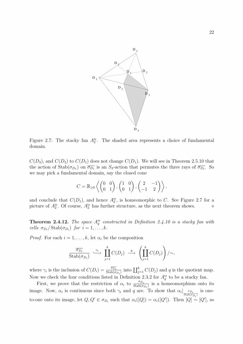
D 4

Figure 2.7: The stacky fan Atr2 . The shaded area represents a choice of fundamental

domain.

C(D3), and C(D4) to C(D1) does not change C(D1). We will see in Theorem 2.5.10 thatthe action of Stab(σD1) on σD1 is an S3-action that permutes the three rays of σD1 . Sowe may pick a fundamental domain, say the closed cone

C = R≥0

⟨(0 00 1

),

(1 00 1

),

(2 −1−1 2

)⟩,

and conclude that C(D1), and hence Atr2 , is homeomorphic to C. See Figure 2.7 for a

picture of Atr2 . Of course, Atr

2 has further structure, as the next theorem shows. ⋄

Theorem 2.4.12. The space Atrg constructed in Definition 2.4.10 is a stacky fan with

cells σDi/ Stab(σDi

) for i = 1, . . . , k.

Proof. For each i = 1, . . . , k, let αi be the composition

σDi

Stab(σDi)

γi

−→k∐

j=1

C(Dj)q

−→

(k∐

j=1

C(Dj)

)/∼,

where γi is the inclusion of C(Di) =σDi

Stab(σDi)

into∐k

j=1C(Dj) and q is the quotient map.

Now we check the four conditions listed in Definition 2.3.2 for Atrg to be a stacky fan.

First, we prove that the restriction of αi toσDi

Stab(σDi)

is a homeomorphism onto its

image. Now, αi is continuous since both γi and q are. To show that αi| σDiStab(σDi

)

is one-

to-one onto its image, let Q,Q′ ∈ σDisuch that αi([Q]) = αi([Q

′]). Then [Q] ∼ [Q′], so

23

there exists A ∈ GLg(Z) such that Q′ = ATQA. Hence Q′ ∈ ATσDiA = σA−1Di

. ThusσA−1Di

and σDiintersect, hence σA−1Di

= σDiand A ∈ Stab(σDi

). So [Q] = [Q′].Thus, αi| σDi

Stab(σDi)

has a well-defined inverse map, and we wish to show that this inverse

map is continuous. Let X ⊆σDi

StabσDi

be closed; we wish to show that αi(X) is closed in

αi

(σDi

StabσDi

). Write X = Y ∩

σDi

StabσDi

where Y ⊆σDi

StabσDi

is closed. Then

αi(X) = αi(Y ) ∩ αi

(σDi

StabσDi

);

this follows from the fact thatGLg(Z)-equivalence never identifies a point on the boundaryof a closed cone with a point in the relative interior. So we need only show that αi(Y ) is

closed in Atrg . To be clear: we want to show that given any closed Y ⊆

σDi

StabσDi

, the image

αi(Y ) ⊆ Atrg is closed.

Let Y ⊆ σDibe the preimage of Y under the quotient map

σDi−։

σDi

StabσDi

.

Then, for each j = 1, . . . , k, let

Yj = {Q ∈ σDj: Q ≡GLg(Z) Q

′ for some Q′ ∈ Y } ⊆ σDj.

We claim each Yj is closed in σDj. First, notice that for any A ∈ GLg(Z), the cone

ATσDiA intersects σDj

in a (closed) face of σDj(after all, the cones form a polyhedral

subdivision). In other words, A defines an integral-linear isomorphism LA : FA,i → FA,jsending X 7→ ATXA, where FA,i is a face of σDi

and FA,j is a face of σDj. Moreover, the

map LA is entirely determined by three choices: the choice of FA,i, the choice of FA,j, andthe choice of a bijection between the rays of FA,i and FA,j. Thus there exist only finitelymany distinct such maps. Therefore

Yj =⋃

A∈GLg(Z)

LA(Y ∩ FA,i) =s⋃

k=1

LAk(Y ∩ FAk,i)

for some choice of finitely many matrices A1, . . . , As ∈ GLg(Z). Now, each LA is ahomeomorphism, so each LA(Y ∩FA,i) is closed in FA,j and hence in σDj

. So Yj is closed.

Finally, let Yj be the image of Yj ⊆ σDjunder the quotient map

σDj

πi

−։

σDj

StabσDj

.

Since π−1j (Yj) = Yj, we have that Yj is closed. Then the inverse image of αi(Y ) under the

quotient mapk∐

j=1

C(Dj) −→

(k∐

j=1

C(Dj)

)/∼

24

is precisely Y1

∐· · ·∐Yk, which is closed. Hence αi(Y ) is closed. This finishes the proof

that αi| σDiStab(σDi

)

is a homeomorphism onto its image.

Property (ii) of being a stacky fan follows from the fact that any matrix Q ∈ Sg≥0 isGLg(Z)-equivalent only to some matrices in a single chosen cone, say σDi

, and no others.Here, Del(Q) and Di are GLg(Z)-equivalent. Thus, given a point in Atr

g represented

by Q ∈ Sg≥0, Q lies in αi

(σDi

StabσDi

)and no other αj

(σDj

StabσDj

), and is the image of a

single point inσDi

StabσDi

since αi was shown to be bijective onσDi

StabσDi

. This shows that

Atrg =

∐ki=1 αi

(σDi

StabσDi

)as a set.

Third, a face F of some cone σDiis σD(F ), where D(F ) is a Delone subdivision that

is a coarsening of Di [Val03, Proposition 2.6.1]. Then there exists Dj and A ∈ GLg(Z)

with σD(F ) · A = σDj(recall that A acts on a point p ∈ Sg≥0 by p 7→ ATpA). Restricting

A to the linear span of σD(F ) gives a linear map

LA : span(σD(F )) −→ span(σDj)

with the desired properties. Note, therefore, that σDkis a stacky face of σDi

precisely ifDk is GLg(Z)-equivalent to a coarsening of Di.

The fourth property then follows: the intersection

αi(σDi) ∩ αj(σDj

) =⋃

αk(σDk)

where σDkranges over all common stacky faces.

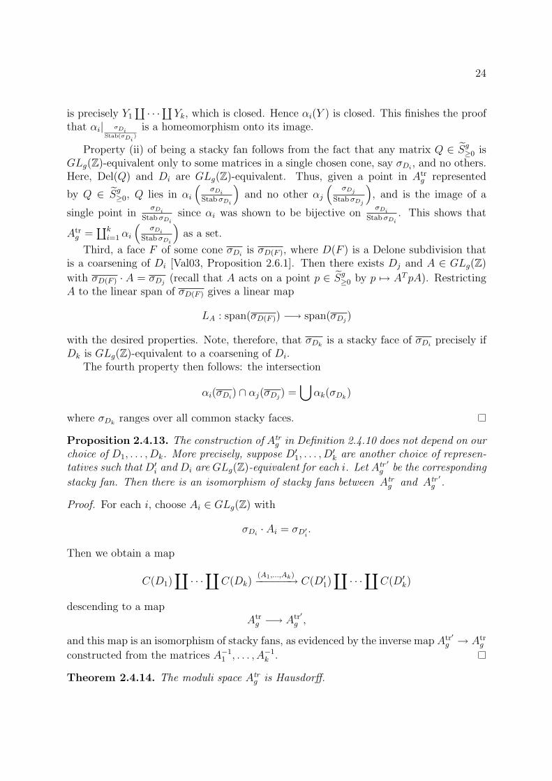
Proposition 2.4.13. The construction of Atrg in Definition 2.4.10 does not depend on our

choice of D1, . . . , Dk. More precisely, suppose D′1, . . . , D

′k are another choice of represen-

tatives such that D′i and Di are GLg(Z)-equivalent for each i. Let Atr ′

g be the corresponding

stacky fan. Then there is an isomorphism of stacky fans between Atrg and Atr ′

g .

Proof. For each i, choose Ai ∈ GLg(Z) with

σDi· Ai = σD′

i.

Then we obtain a map

C(D1)∐

· · ·∐

C(Dk)(A1,...,Ak)−−−−−−→ C(D′

1)∐

· · ·∐

C(D′k)

descending to a mapAtrg −→ Atr′

g ,

and this map is an isomorphism of stacky fans, as evidenced by the inverse map Atr′

g → Atrg

constructed from the matrices A−11 , . . . , A−1

k .

Theorem 2.4.14. The moduli space Atrg is Hausdorff.

25

Remark 2.4.15. Theorem 2.4.14 complements the theorem of Caporaso that M trg is

Hausdorff [Cap10, Theorem 5.2].

Proof. Let σD1 , . . . , σDkbe representatives for GLg(Z)-classes of secondary cones. Let

us regard Atrg as a quotient of the cones themselves, rather than the cones modulo their

stabilizers, thus

Atrg =

(k∐

i=1

σDk

)/ ∼

where ∼ denotes GLg(Z)-equivalence as usual. Denote by βi the natural maps

βi : σDi−→ Atr

g .

Now suppose p 6= q ∈ Atrg . For each i = 1, . . . , k, pick disjoint open sets Ui and Vi in σDi

such that β−1i (p) ⊆ Ui and β−1

i (q) ⊆ Vi. Let

U := {x ∈ Atrg : β−1

i (x) ⊆ Ui for all i},

V := {x ∈ Atrg : β−1

i (x) ⊆ Vi for all i}.

By construction, we have p ∈ U and q ∈ V . We claim that U and V are disjoint opensets in Atr

g .

Suppose x ∈ U ∩ V . Now β−1i (x) is nonempty for some i, hence Ui ∩ Vi is nonempty,

contradiction. Hence U and V are disjoint. So we just need to prove that U is open(similarly, V is open). It suffices to show that for each j = 1, . . . , k, the set β−1

j (U) isopen. Now,

β−1j (U) = {y ∈ σDj

: β−1i βj(y) ⊆ Ui for all i},

=⋂

i

{y ∈ σDj: β−1

i βj(y) ⊆ Ui}.

Write Uij for the sets in the intersection above, so that β−1j (U) =

⋂i Uij, and let

Zi = σDi\Ui. Note that Uij consists of those points in σDj

that are not GLg(Z)-equivalentto any point in Zi. Then, just as in the proof of Theorem 2.4.12, there exist finitely manymatrices A1, . . . , As ∈ GLg(Z) such that

σDj\ Uij = {y ∈ σDj

: y ∼ z for some z ∈ Zi}

=s⋃

l=1

(ATl ZiAl ∩ σDj

),

which shows that σDj\ Uij is closed. Thus the Uij’s are open and so β−1

j (U) is open foreach j. Hence U is open, and similarly, V is open.

Remark 2.4.16. Actually, we could have done a much more general construction ofAtrg . We made a choice of decomposition of Sg≥0: we chose the second Voronoi decom-

position, whose cones are secondary cones of Delone subdivisions. This decomposition

26

has the advantage that it interacts nicely with the Torelli map, as we will see. But, asrightly pointed out in [BMV11], we could use any decomposition of Sg≥0 that is “GLg(Z)-

admissible.” This means that it is an infinite polyhedral subdivision of Sg≥0 such thatGLg(Z) permutes its open cones in a finite number of orbits. See [AMRT75, Section II]for the formal definition. Every result in this section can be restated for a general GLg(Z)-admissible decomposition: each such decomposition produces a moduli space which is astacky fan, which is independent of any choice of representatives, and which is Hausdorff.The proofs are all the same. Here, though, we chose to fix a specific decomposition purelyfor the sake of concreteness and readability, invoking only what we needed to build up tothe definition of the Torelli map.

§2.4.4 The quotient space Sg

≥0/GLg(Z)

We briefly remark on the construction of Atrg originally proposed in [BMV11]. There,

the strategy is to try to equip the quotient space Sg≥0/GLg(Z) directly with a stacky fanstructure. To do this, one maps a set of representative cones σD, modulo their stabilizersStab(σD), into the space Sg≥0/GLg(Z), via the map

iD : σD/ Stab(σD) → Sg≥0/GLg(Z)

induced by the inclusion σD → Sg≥0.The problem is that the map iD above may not be a homeomorphism onto its image.

In fact, the image of σD/ Stab(σD) in Sg≥0/GLg(Z) may not even be Hausdorff, eventhough σD/ Stab(σD) certainly is. The following example shows that the cone σD3 , usingthe notation of Example 2.4.11, exhibits such behavior. Note that Stab(σD3) happens tobe trivial in this case.

Example 2.4.17. Let {Xn}n≥1 and {Yn}n≥1 be the sequences of matrices

Xn =

(1 1

n1n

1n2

), Yn =

(1n2 00 0

)

in S2≥0. Then we have

{Xn} →

(1 00 0

), {Yn} →

(0 00 0

).

On the other hand, for each n, Xn ≡GL2(Z) Yn even while ( 1 00 0 ) 6≡GL2(Z) ( 0 0

0 0 ). This ex-ample then descends to non-Hausdorffness in the topological quotient. It can easily begeneralized to g > 2. ⋄

Thus, we disagree with the claim in the proof of Theorem 4.2.4 of [BMV11] thatthe open cones σD, modulo their stabilizers, map homeomorphically onto their image inSg≥0/GLg(Z). However, we emphasize that our construction in Section 4.3 is just a minormodification of the ideas already present in [BMV11].

27

2.5 Regular matroids and the zonotopal subfan

In the previous section, we defined the moduli space Atrg of principally polarized tropical

abelian varieties. In this section, we describe a particular stacky subfan of Atrg whose cells

are in correspondence with simple regular matroids of rank at most g. This subfan iscalled the zonotopal subfan and denoted Azon

g because its cells correspond to those classesof Delone triangulations which are dual to zonotopes; see [BMV11, Section 4.4]. Thezonotopal subfan Azon

g is important because, as we shall see in Section 6, it contains theimage of the Torelli map. For g ≥ 4, this containment is proper. Our main contributionin this section is to characterize the stabilizing subgroups of all zonotopal cells.

We begin by recalling some basic facts about matroids. A good reference is [Oxl92].The connection between matroids and the Torelli map seems to have been first observedby Gerritzen [Ger82], and our approach here can be seen as an continuation of his workin the late 1970s.

Definition 2.5.1. A matroid is said to be simple if it has no loops and no parallelelements.

Definition 2.5.2. A matroid M is regular if it is representable over every field; equiv-alently, M is regular if it is representable over R by a totally unimodular matrix. (Atotally unimodular matrix is a matrix such that every square submatrix has determinantin {0, 1,−1}.)

Next, we review the correspondence between simple regular matroids and zonotopalcells.

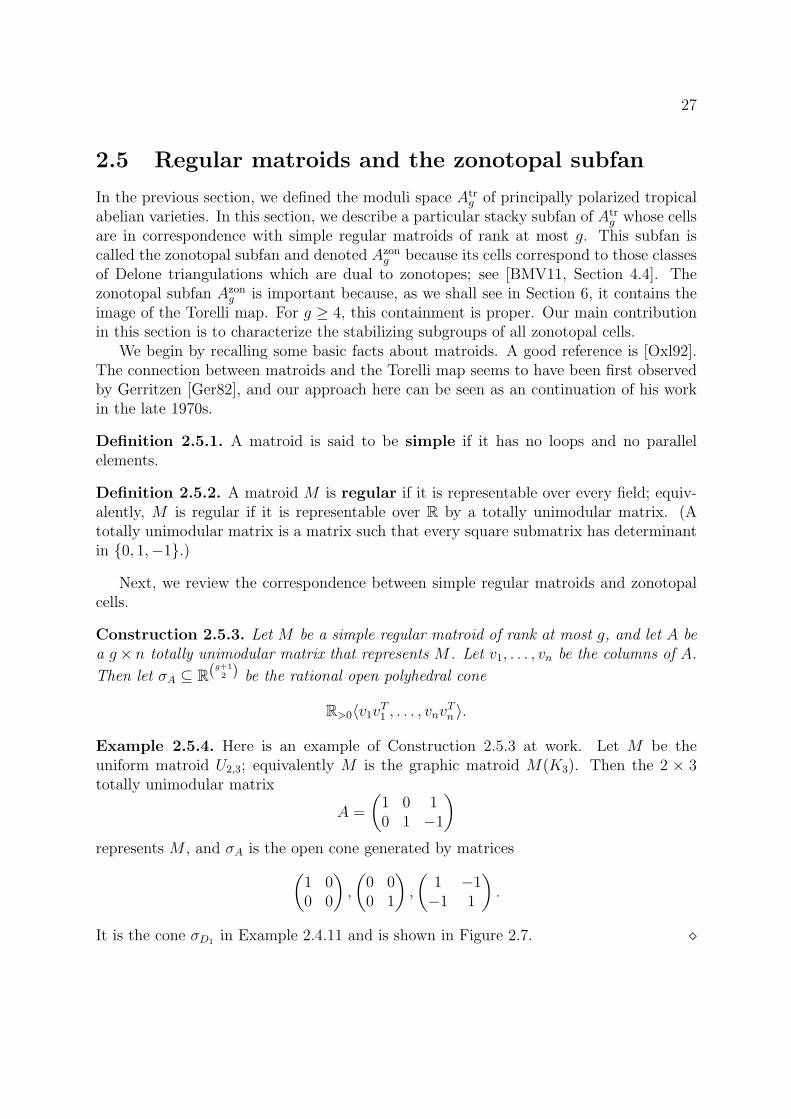
Construction 2.5.3. Let M be a simple regular matroid of rank at most g, and let A bea g× n totally unimodular matrix that represents M . Let v1, . . . , vn be the columns of A.

Then let σA ⊆ R(g+12 ) be the rational open polyhedral cone

R>0〈v1vT1 , . . . , vnv

Tn 〉.

Example 2.5.4. Here is an example of Construction 2.5.3 at work. Let M be theuniform matroid U2,3; equivalently M is the graphic matroid M(K3). Then the 2 × 3totally unimodular matrix

A =

(1 0 10 1 −1

)

represents M , and σA is the open cone generated by matrices

(1 00 0

),

(0 00 1

),

(1 −1−1 1

).

It is the cone σD1 in Example 2.4.11 and is shown in Figure 2.7. ⋄

28

Proposition 2.5.5. [BMV11, Lemma 4.4.3, Theorem 4.4.4] Let M be a simple regularmatroid of rank at most g, and let A be a g×n totally unimodular matrix that representsM . Then the cone σA, defined in Construction 2.5.3, is a secondary cone in Sg≥0. Choos-ing a different totally unimodular matrix A′ to represent M produces a cone σA′ that isGLg(Z)-equivalent to σA. Thus, we may associate to M a unique cell of Atr

g , denotedC(M).

Definition 2.5.6. The zonotopal subfan Azong is the union of cells in Atr

g

Azong =

⋃

M a simple regularmatroid of rank ≤ g

C(M).

We briefly recall the definition of the Voronoi polytope of a quadratic form in Sg≥0,just in order to explain the relationship with zonotopes.

Definition 2.5.7. Let Q ∈ Sg≥0, and let H = (kerQ)⊥ ⊆ Rg. Then

Vor(Q) = {x ∈ H : xTQx ≤ (x− λ)TQ(x− λ) ∀λ ∈ Zg}

is a polytope in H ⊆ Rg, called the Voronoi polytope of Q.

Theorem 2.5.8. [BMV11, Theorem 4.4.4, Definition 4.4.5] The zonotopal subfan Azong

is a stacky subfan of Atrg . It consists of those points of the tropical moduli space Atr

g whoseVoronoi polytope is a zonotope.

Remark 2.5.9. Suppose σ is an open rational polyhedral cone in Rn. Then any A ∈GLn(Z) such that Aσ = σ must permute the rays of σ, since the action of A on σ islinear. Furthermore, it sends a first lattice point on a ray to another first lattice point;that is, it preserves lattice lengths. Thus, the subgroup Stab(σ) ⊆ GLn(Z) realizes somesubgroup of the permutation group on the rays of σ (although if σ is not full-dimensionalthen the action of Stab(σ) on its rays may not be faithful).

Now, given a simple regular matroid M of rank ≤ g, we have almost computed thecell of Atr

g to which it corresponds. Specifically, we have computed the cone σA for Aa matrix representing M , in Construction 2.5.3. The remaining task is to compute theaction of the stabilizer Stab(σA).

Note that σA has rays corresponding to the columns of A: a column vector vi corre-sponds to the ray generated by the symmetric rank 1 matrix viv

Ti . In light of Remark

2.5.9, we might conjecture that the permutations of rays of σA coming from the stabilizerare the ones that respect the matroid M , i.e. come from matroid automorphisms. Thatis precisely the case and provides valuable local information about Atr

g .

Theorem 2.5.10. Let A be a g × n totally unimodular matrix representing the simpleregular matroid M . Let H denote the group of permutations of the rays of σA which arerealized by the action of Stab(σA). Then

H ∼= Aut(M).

29

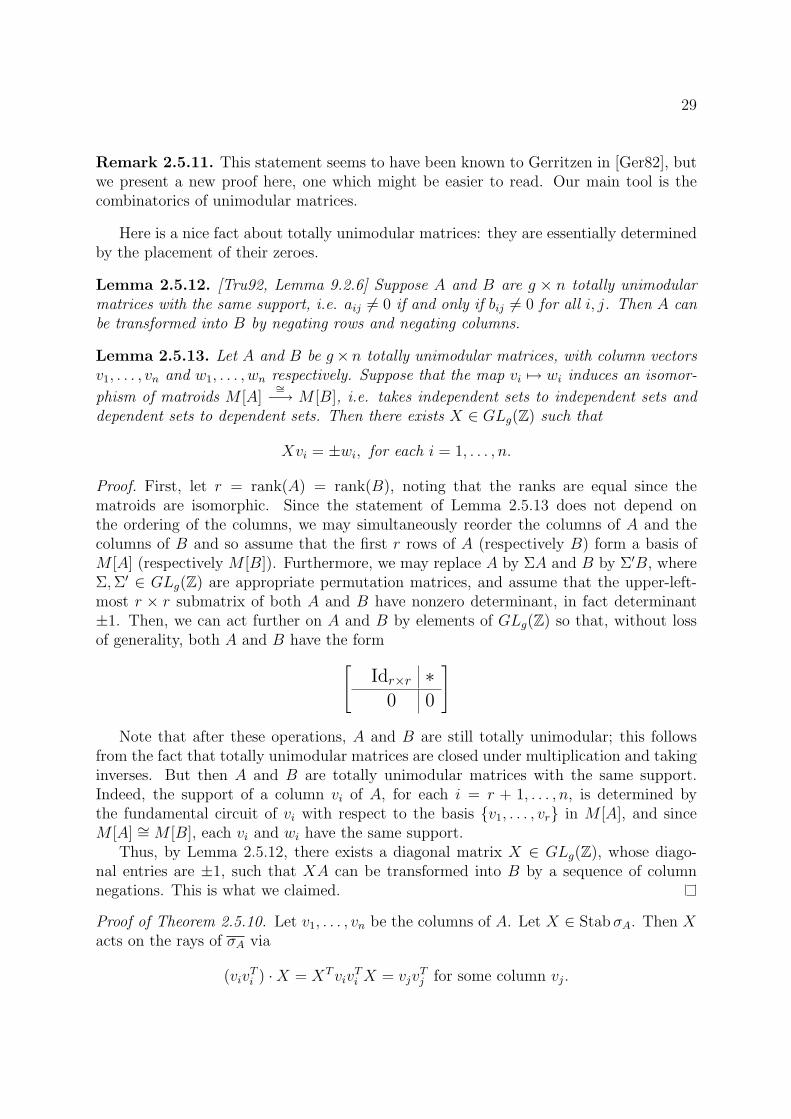
Remark 2.5.11. This statement seems to have been known to Gerritzen in [Ger82], butwe present a new proof here, one which might be easier to read. Our main tool is thecombinatorics of unimodular matrices.

Here is a nice fact about totally unimodular matrices: they are essentially determinedby the placement of their zeroes.

Lemma 2.5.12. [Tru92, Lemma 9.2.6] Suppose A and B are g × n totally unimodularmatrices with the same support, i.e. aij 6= 0 if and only if bij 6= 0 for all i, j. Then A canbe transformed into B by negating rows and negating columns.

Lemma 2.5.13. Let A and B be g× n totally unimodular matrices, with column vectorsv1, . . . , vn and w1, . . . , wn respectively. Suppose that the map vi 7→ wi induces an isomor-

phism of matroids M [A]∼=

−→ M [B], i.e. takes independent sets to independent sets anddependent sets to dependent sets. Then there exists X ∈ GLg(Z) such that

Xvi = ±wi, for each i = 1, . . . , n.

Proof. First, let r = rank(A) = rank(B), noting that the ranks are equal since thematroids are isomorphic. Since the statement of Lemma 2.5.13 does not depend onthe ordering of the columns, we may simultaneously reorder the columns of A and thecolumns of B and so assume that the first r rows of A (respectively B) form a basis ofM [A] (respectively M [B]). Furthermore, we may replace A by ΣA and B by Σ′B, whereΣ,Σ′ ∈ GLg(Z) are appropriate permutation matrices, and assume that the upper-left-most r × r submatrix of both A and B have nonzero determinant, in fact determinant±1. Then, we can act further on A and B by elements of GLg(Z) so that, without lossof generality, both A and B have the form

[Idr×r ∗

0 0

]

Note that after these operations, A and B are still totally unimodular; this followsfrom the fact that totally unimodular matrices are closed under multiplication and takinginverses. But then A and B are totally unimodular matrices with the same support.Indeed, the support of a column vi of A, for each i = r + 1, . . . , n, is determined bythe fundamental circuit of vi with respect to the basis {v1, . . . , vr} in M [A], and sinceM [A] ∼= M [B], each vi and wi have the same support.

Thus, by Lemma 2.5.12, there exists a diagonal matrix X ∈ GLg(Z), whose diago-nal entries are ±1, such that XA can be transformed into B by a sequence of columnnegations. This is what we claimed.

Proof of Theorem 2.5.10. Let v1, . . . , vn be the columns of A. Let X ∈ StabσA. Then Xacts on the rays of σA via

(vivTi ) ·X = XTviv

Ti X = vjv

Tj for some column vj.

30

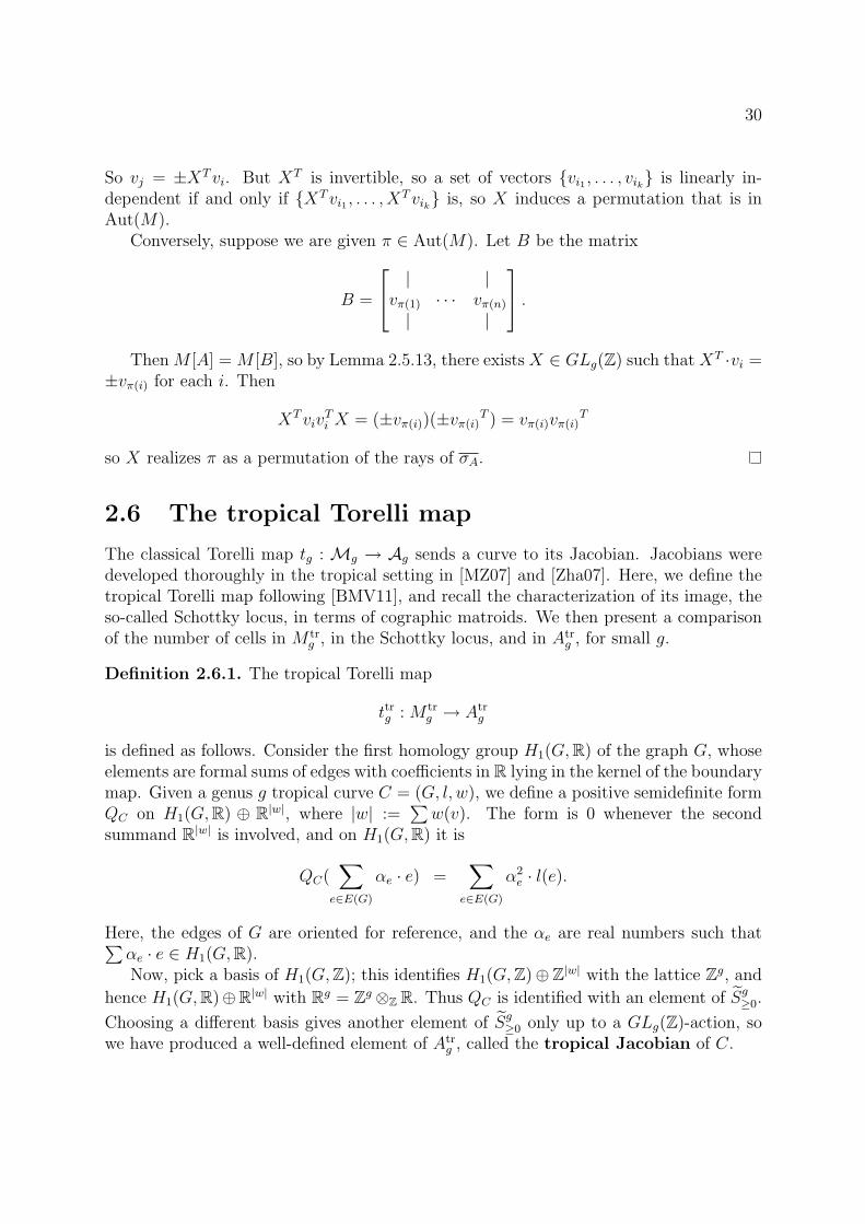
So vj = ±XTvi. But XT is invertible, so a set of vectors {vi1 , . . . , vik} is linearly in-dependent if and only if {XTvi1 , . . . , X

Tvik} is, so X induces a permutation that is inAut(M).

Conversely, suppose we are given π ∈ Aut(M). Let B be the matrix

B =

| |vπ(1) · · · vπ(n)

| |

.

Then M [A] = M [B], so by Lemma 2.5.13, there existsX ∈ GLg(Z) such that XT ·vi =±vπ(i) for each i. Then

XTvivTi X = (±vπ(i))(±vπ(i)

T ) = vπ(i)vπ(i)T

so X realizes π as a permutation of the rays of σA.

2.6 The tropical Torelli map

The classical Torelli map tg : Mg → Ag sends a curve to its Jacobian. Jacobians weredeveloped thoroughly in the tropical setting in [MZ07] and [Zha07]. Here, we define thetropical Torelli map following [BMV11], and recall the characterization of its image, theso-called Schottky locus, in terms of cographic matroids. We then present a comparisonof the number of cells in M tr

g , in the Schottky locus, and in Atrg , for small g.

Definition 2.6.1. The tropical Torelli map

ttrg : M trg → Atr

g

is defined as follows. Consider the first homology group H1(G,R) of the graph G, whoseelements are formal sums of edges with coefficients in R lying in the kernel of the boundarymap. Given a genus g tropical curve C = (G, l, w), we define a positive semidefinite formQC on H1(G,R) ⊕ R|w|, where |w| :=

∑w(v). The form is 0 whenever the second

summand R|w| is involved, and on H1(G,R) it is

QC(∑

e∈E(G)

αe · e) =∑

e∈E(G)

α2e · l(e).

Here, the edges of G are oriented for reference, and the αe are real numbers such that∑αe · e ∈ H1(G,R).Now, pick a basis of H1(G,Z); this identifies H1(G,Z)⊕Z|w| with the lattice Zg, and

hence H1(G,R)⊕R|w| with Rg = Zg ⊗Z R. Thus QC is identified with an element of Sg≥0.

Choosing a different basis gives another element of Sg≥0 only up to a GLg(Z)-action, sowe have produced a well-defined element of Atr

g , called the tropical Jacobian of C.

31

Theorem 2.6.2. [BMV11, Theorem 5.1.5] The map

ttrg : M trg → Atr

g

is a morphism of stacky fans.

Note that the proof by Brannetti, Melo, and Viviani of Theorem 2.6.2 is correct underthe new definitions. In particular, the definition of a morphism of stacky fans has notchanged.

The following theorem tells us how the tropical Torelli map behaves, at least on thelevel of stacky cells. Given a graph G, its cographic matroid is denoted M∗(G), and

M∗(G) is then the matroid obtained by removing loops and replacing each parallel classwith a single element. See [BMV11, Definition 2.3.8].

Theorem 2.6.3. [BMV11, Theorem 5.1.5] The map ttrg sends the cell C(G,w) of M trg

surjectively to the cell C(M∗(G)).

We denote by Acogrg the stacky subfan of Atr

g consisting of those cells

{C(M) : M a simple cographic matroid of rank ≤ g}.

The cell C(M) was defined in Construction 2.5.3. Note that Acogrg sits inside the zonotopal

subfan of Section 5:Acogrg ⊆ Azon

g ⊆ Atrg .

Also, Acogrg = Atr

g when g ≤ 3, but not when g ≥ 4 ([BMV11, Remark 5.2.5]). Theprevious theorem says that the image of ttrg is precisely Acogr

g ⊆ Atrg . So, in analogy with

the classical situation, we call Acogrg the tropical Schottky locus.

Figures 2.1 and 2.8 illustrate the tropical Torelli map in genus 3. The cells of M tr3 in

Figure 2.1 are color-coded according to the color of the cells of Atr3 in Figure 2.8 to which

they are sent. These figures serve to illustrate the correspondence in Theorem 2.6.3.Our contribution in this section is to compute the poset of cells of Acogr

g , for g ≤ 5,using Mathematica. First, we computed the cographic matroid of each graph of genus≤ g, and discarded the ones that were not simple. Then we checked whether any twomatroids obtained in this way were in fact isomorphic. Part of this computation wasdone by hand in the genus 5 case, because it became intractable to check whether two12-element matroids were isomorphic. Instead, we used some heuristic tests and thenchecked by hand that, for the few pairs of matroids passing the tests, the original pair ofgraphs were related by a sequence of vertex-cleavings and Whitney flips. This conditionensures that they have the same cographic matroid; see [Oxl92].

Theorem 2.6.4. We obtained the following computational results:

(i) The tropical Schottky locus Acogr3 has nine cells and f -vector

(1, 1, 1, 2, 2, 1, 1).

Its poset of cells is shown in Figure 2.8.

32

.Figure 2.8: Poset of cells of Atr

3 = Acogr3 . Each cell corresponds to a cographic matroid,

and for convenience, we draw a graph G in order to represent its cographic matroidM∗(G).

33

(ii) The tropical Schottky locus Acogr4 has 25 cells and f -vector

(1, 1, 1, 2, 3, 4, 5, 4, 2, 2).

(iii) The tropical Schottky locus Acogr5 has 92 cells and f -vector

(1, 1, 1, 2, 3, 5, 9, 12, 15, 17, 15, 7, 4).

Remark 2.6.5. Actually, since Acogr3 = Atr

3 , the results of part (i) of Theorem 2.6.4 werealready known, say in [Val03].

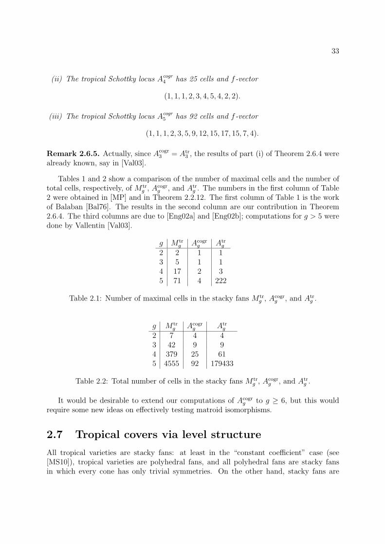
Tables 1 and 2 show a comparison of the number of maximal cells and the number oftotal cells, respectively, of M tr

g , Acogrg , and Atr

g . The numbers in the first column of Table2 were obtained in [MP] and in Theorem 2.2.12. The first column of Table 1 is the workof Balaban [Bal76]. The results in the second column are our contribution in Theorem2.6.4. The third columns are due to [Eng02a] and [Eng02b]; computations for g > 5 weredone by Vallentin [Val03].

g M trg Acogr

g Atrg

2 2 1 13 5 1 14 17 2 35 71 4 222

Table 2.1: Number of maximal cells in the stacky fans M trg , Acogr

g , and Atrg .

g M trg Acogr

g Atrg

2 7 4 43 42 9 94 379 25 615 4555 92 179433

Table 2.2: Total number of cells in the stacky fans M trg , Acogr

g , and Atrg .

It would be desirable to extend our computations of Acogrg to g ≥ 6, but this would

require some new ideas on effectively testing matroid isomorphisms.

2.7 Tropical covers via level structure

All tropical varieties are stacky fans: at least in the “constant coefficient” case (see[MS10]), tropical varieties are polyhedral fans, and all polyhedral fans are stacky fansin which every cone has only trivial symmetries. On the other hand, stacky fans are

34

not always tropical varieties. Indeed, one problem with the spaces M trg and Atr

g is thatalthough they are tropical moduli spaces, they do not “look” very tropical: they do notsatisfy a tropical balancing condition (see [MS10]).

But what if we allow ourselves to consider finite-index covers of our spaces – can wethen produce a more tropical object? In what follows, we answer this question for thespaces Atr

2 and Atr3 . The uniform matroid U2

4 and the Fano matroid F7 play a role. Weare grateful to Diane Maclagan for suggesting this question and the approach presentedhere.

Given n ≥ 1, let FPn denote the complete polyhedral fan in Rn associated to projectivespace Pn, regarded as a toric variety. Concretely, we fix the rays of FPn to be generatedby

e1, . . . , en, en+1 := −e1 − · · · − en,

and each subset of at most n rays spans a cone in FPn. So FPn has n+1 top-dimensionalcones. Given S ⊆ {1, . . . , n+1}, let cone(S) denote the open cone R>0{ei : i ∈ S} in FPn,let cone(ı) := cone({1, . . . , ı, . . . , n+1}), and let cone(S) be the closed cone correspondingto S. Note that the polyhedral fan FPn is also a stacky fan: each open cone can beequipped with trivial symmetries. Its support is the tropical variety corresponding to allof Tn.

By a generic point of Atrg , we mean a point x lying in a cell of Atr

g of maximaldimension such that any positive semidefinite matrix X representing x is fixed only bythe identity element in GLg(Z).

§2.7.1 A tropical cover for Atr

3

By the classification in Sections 4.1–4.3 of [Val03], we note that

Atr3 =

(∐

M⊆MK4

C(M)

)/ ∼ .

In the disjoint union above, the symbol MK4 denotes the graphic (equivalently, in thiscase, cographic) matroid of the graph K4, and M ⊆ M ′ means that M is a submatroidof M ′, i.e. obtained by deleting elements. The cell C(M) of a regular matroid M wasdefined in Construction 2.5.3. There is a single maximal cell C(MK4) in Atr

3 , and theother cells are stacky faces of it. The cells are also listed in Figure 2.8.

Now define a continuous map

π : FP6 → Atr3

as follows. Let A be a 3 × 6 unimodular matrix representing MK4, for example

A =

1 0 0 1 1 00 1 0 −1 0 10 0 1 0 −1 −1

,

35

and let σA be the cone in S3≥0 with rays {viv

Ti }, where the vi’s are the columns of A, as in

Construction 2.5.3. Fix, once and for all, a Fano matroid structure on the set {1, . . . , 7}.For example, we could take F7 to have circuits {124, 235, 346, 457, 156, 267, 137}.

Now, for each i = 1, . . . , 7, the deletion F7 \ {i} is isomorphic to MK4, so let

πı : [7] \ {i} → E(MK4)

be any bijection inducing such an isomorphism. Now define

αı : cone(ı) → Atr3

as the composition

cone(ı)Lı−−→ σA −։

σAStabσA

= C(MK4) −→ Atr3

where Lı is the integral-linear map arising from πı.Now, each αı is clearly continuous, and to paste them together into a map on all

of FP6, we need to show that they agree on intersections. Thus, fix i 6= j and letS ⊆ {1, . . . , 7} \ {i, j}. We want to show that

αı = α on cone(S).

Indeed, the map Lı sends cone(S) isomorphically to σA|πı(S), where A|πı(S) denotes

the submatrix of A gotten by taking the columns indexed by πı(S). Furthermore, thebijection on the rays of the cones agrees with the isomorphism of matroids

F7|S∼=

−−−→MK4|πı(S).

Similarly, L sends cone(S) isomorphically to σA|π(S), and the map on rays agrees with

the matroid isomorphism

F7|S∼=

−−−→MK4|π(S).

Hence MK4|πı(S)∼= MK4|π(S) and by Theorem 2.5.10, there exists X ∈ GL3(Z) such

that the diagram commutes:

σA|πı(S)

X

��

cone(S)

Lı

66mmmmmmmmmmmm

L

((PPPPPPPPPPPPPP

σA|π(S)

We conclude that αı and α agree on cone(S), since Lı and L differ only by a GL3(Z)-action.

Therefore, we can glue the seven maps αı together to obtain a continuous map α :FP6 → Atr

3 .

36

Theorem 2.7.1. The map α : FP6 → Atr3 is a surjective morphism of stacky fans.

Each of the seven maximal cells of FP6 is mapped surjectively onto the maximal cell ofAtr

3 . Furthermore, the map α has finite fibers, and if x ∈ Atr3 is a generic point, then

|α−1(x)| = 168.

Proof. By construction, α sends each cell cone(S) of FP6 surjectively onto the cell of Atr3

corresponding to the matroid F7|S, and each of these maps is induced by some integral-linear map Lı. That α is surjective then follows from the fact that every submatroid ofMK4 is a proper submatroid of F7. Also, by construction, α maps each maximal cellcone(ı) of FP6 surjectively to the cell C(MK4) of Atr

3 .By definition of the map αi, each x ∈ Atr

3 has only finitely many preimages α−1i (x) in

cone(ı), so α has finite fibers. If x ∈ Atr3 is a generic point, then x has 24 = |Aut(MK4)|

preimages in each of the seven maximal open cones cone(ı), so |α−1(x)| = 168.

§2.7.2 A tropical cover for Atr

2

Our strategy in Theorem 2.7.1 for constructing a covering map FP6 → Atr3 was to use the

combinatorics of the Fano matroid to paste together seven copies of MK4 in a coherentway. In fact, an analogous, and easier, argument yields a covering map FP3 → Atr

2 . Wewill use U2

4 to paste together four copies of U23 . Here, Ud

n denotes the uniform rank dmatroid on n elements.

The space Atr2 can be given by

Atr2 =

∐

M⊆U23

C(M)

/ ∼ .

It has a single maximal cell C(U23 ), and the three other cells are stacky faces of it of

dimensions 0, 1, and 2. See Figure 2.7.Analogously to Section 7.1, let

A =

(1 0 10 1 −1

),

say, and for each i = 1, . . . , 4, define

βı : cone(ı) → Atr2

by sending cone(ı) to σA by a bijective linear map preserving lattice points. Here, any ofthe 3! possible maps will do, because the matroid U2

3 has full automorphisms.Just as in Section 7.1, we may check that the four maps αı agree on their overlaps, so

we obtain a continuous mapβ : FP3 → Atr

2 .

37

Proposition 2.7.2. The map β : FP3 → Atr2 is a surjective morphism of stacky fans.

Each of the four maximal cells of FP3 maps surjectively onto the maximal cell of Atr2 .

Furthermore, the map β has finite fibers, and if x ∈ Atr2 is a generic point, then we have

|β−1(x)| = 24.

Proof. The proof is exactly analogous to the proof of Theorem 2.7.1. Instead of notingthat every one-element deletion of F7 is isomorphic toMK4, we make the easy observationthat every one-element deletion of U2

4 is isomorphic to U23 . If x ∈ Atr

2 is a generic point,then x has 6 = |Aut(U2

3 )| preimages in each of the four maximal open cones of FP3.

Remark 2.7.3. We do not know a more general construction for g ≥ 4. We seem to berelying on the fact that all cells of Atr

g are cographic when g = 2, 3, but this is not truewhen g ≥ 4: the Schottky locus is proper.

Remark 2.7.4. Although our constructions look purely matroidal, they come from levelstructures on Atr

2 and Atr3 with respect to the primes p = 3 and p = 2, respectively. More

precisely, in the genus 2 case, consider the decomposition of S2≥0 into secondary cones as

in Theorem 2.4.7, and identify rays vvT and wwT if v ≡ ±w (mod 3). Then we obtainFP3. The analogous statement holds, replacing the prime 3 with 2, in genus 3.

38

Chapter 3

Tropical hyperelliptic curves

This chapter covers the material in [Cha11b], which will appear in the Journal ofAlgebraic Combinatorics, with only minor changes in wording.

3.1 Introduction

Our aim in this chapter is to study the locus of hyperelliptic curves inside the moduli spaceof tropical curves of a fixed genus g. Our work ties together two strands in the recent trop-ical geometry literature: tropical Brill-Noether theory on the one hand [Bak08], [Cap11b],[CDPR10], [LPP11]; and tropical moduli spaces of curves on the other [BMV11], [Cap10],[Cap11a], [Cha11a], [MZ07].

The work of Baker and Norine in [BN07] and Baker in [Bak08] has opened up a world offascinating connections between algebraic and tropical curves. The Specialization Lemmaof Baker [Bak08], recently extended by Caporaso [Cap11b], allows for precise translationsbetween statements about divisors on algebraic curves and divisors on tropical curves.One of its most notable applications is to tropical Brill-Noether theory. The classicalBrill-Noether theorem in algebraic geometry, proved by Griffiths and Harris, [GH80], isthe following.

Theorem 3.1.1. Suppose g, r, and d are positive numbers and let

ρ(g, r, d) = g − (r + 1)(g − d+ r).

(i) If ρ ≥ 0, then every smooth projective curve X of genus g has a divisor of degreed and rank at least r. In fact, the scheme W r

d (X) parametrizing linear equivalenceclasses of such divisors has dimension min{ρ, g}.

(ii) If ρ < 0, then the general smooth projective curve of genus g has no divisors ofdegree d and rank at least r.

A tropical proof of the Brill-Noether theorem by way of the Specialization Lemma wasconjectured in [Bak08] and obtained by Cools, Draisma, Payne, and Robeva in [CDPR10].See [Cap11b] and [LPP11] for other advances in tropical Brill-Noether theory.

39

Another strand in the literature concerns the (3g − 3)-dimensional moduli space M trg

of tropical curves of genus g. This space was considered by Mikhalkin and Zharkovin [Mik06b] and [MZ07], in a more limited setting (i.e. without vertex weights). It wasconstructed and studied as a topological space by Caporaso, who proved thatM tr

g is Haus-dorff and connected through codimension one [Cap10], [Cap11a]. In [BMV11], Brannetti,Melo, and Viviani constructed it explicitly in the category of stacky polyhedral fans (seeDefinition 2.3.2). In [Cha11a], we gained a detailed understanding of the combinatoricsof M tr

g , which deeply informs the present study.Fix g, r, and d such that ρ(g, r, d) < 0. Then the Brill-Noether locus Mr

g,d ⊂ Mg

consists of those genus g curves which are exceptional in Theorem 3.1.1(ii) in the sensethat they do admit a divisor of degree d and rank at least r. The tropical Brill-Noetherlocus M r,tr

g,d ⊂M trg is defined in exactly the same way.

In light of the recent advances in both tropical Brill-Noether theory and tropicalmoduli theory, it is natural to pose the following

Problem 3.1.2. Characterize the tropical Brill-Noether loci M r,trg,d inside M tr

g .

The case r = 1 and d = 2 is, of course, the case of hyperelliptic curves, and the combi-natorics is already very rich. Here, we are able to characterize the hyperelliptic loci ineach genus. The main results of this chapter are the follwing three theorems, proved inSections 3, 4, and 5, respectively.

Theorem 3.1.3. Let Γ be a metric graph with no points of valence 1, and let (G, l) denoteits canonical loopless model. Then the following are equivalent:

(i) Γ is hyperelliptic.

(ii) There exists an involution i : G→ G such that G/i is a tree.

(iii) There exists a nondegenerate harmonic morphism of degree 2 from G to a tree, or|V (G)| = 2. (See Figure 3.1).

Theorem 3.1.4. Let g ≥ 3. The locus of 2-edge-connected genus g tropical hyperellipticcurves is a (2g−1)-dimensional stacky polyhedral fan whose maximal cells are in bijectionwith trees on g − 1 vertices with maximum valence 3. (See Figure 3.3).

Theorem 3.1.5. Let X ⊆ T2 be a hyperelliptic curve of genus g ≥ 3 over a com-plete, algebraically closed nonarchimedean valuated field K, and suppose X is defined bya polynomial of the form P = y2 + f(x)y + h(x). Let X be its smooth completion. Sup-pose the Newton complex of P is a unimodular subdivision of the triangle with vertices(0, 0), (2g + 2, 0), and (0, 2), and suppose that the core of TropX is bridgeless. Then the

skeleton Σ of the Berkovich analytification Xan is a standard ladder of genus g whoseopposite sides have equal length. (See Figure 3.9).

We begin in Section 2 by giving new definitions of harmonic morphisms and quotientsof metric graphs, and recalling the basics of divisors on tropical curves. In Section 3, we

40

a

a

a

b

c

c

c2b

Figure 3.1: A harmonic morphism of degree two. Here, a, b, and c are positive realnumbers.

prove the characterization of hyperellipticity stated in Theorem 3.1.3. This generalizes acentral result of [BN09] to metric graphs. See also [HMY09, Proposition 45] for a proof ofone of the three parts. In Section 4, we build the space of hyperelliptic tropical curves andthe space of 2-edge-connected hyperelliptic tropical curves. We then explicitly computethe hyperelliptic loci in M tr

g for g = 3 and g = 4. See Figures 3.2 and 3.3. Note that allgenus 2 tropical curves are hyperelliptic, as in the classical case. Finally, in Section 5,we establish a connection to embedded tropical curves in the plane, of the sort shown inFigure 3.9, and prove Theorem 3.1.5.

Our work in Section 5 represents a first step in studying the behavior of hyperellipticcurves under the map

trop : Mg(K) →M trg

in [BPR11, Remark 5.51], which sends a curve X over a algebraically closed, completenonarchimedean field K to its Berkovich skeleton, or equivalently to the dual graph,appropriately metrized, of the special fiber of a semistable model for X. Note thatalgebraic curves that are not hyperelliptic can tropicalize to hyperelliptic curves [Bak08,Example 3.6], whereas tropicalizations of hyperelliptic algebraic curves are necessarilyhyperelliptic [Bak08, Corollary 3.5]. It would be very interesting to study further thebehavior of hyperelliptic loci, and higher Brill-Noether loci, under the tropicalizationmap above.

3.2 Definitions and notation

We start by defining harmonic morphisms, quotients, divisors, and rational functions onmetric graphs. These concepts will be used in Theorem 3.3.12 to characterize hyperellip-ticity.

41

§3.2.1 Metric graphs and harmonic morphisms

Throughout, all of our graphs are connected, with loops and multiple edges allowed. Ametric graph is a metric space Γ such that there exists a graph G and a length function

l : E (G) → R>0

so that Γ is obtained from (G, l) by gluing intervals [0, l (e)] for e ∈ E (G) at theirendpoints, as prescribed by the combinatorial data of G. The distance d (x, y) betweentwo points x and y in Γ is given by the length of the shortest path between them. Wesay that (G, l) is a model for Γ in this case. We say that (G, l) is a loopless model if Ghas no loops. Note that a given metric graph Γ admits many possible models (G, l). Forexample, a line segment of length a can be subdivided into many edges whose lengthssum to a. The reason for working with both metric graphs and models is that metricgraphs do not have a preferred vertex set, but choosing some vertex set is convenient formaking combinatorial statements.

Suppose Γ is a metric graph, and let us exclude, once and for all, the case that Γ ishomeomorphic to the circle S1. We define the valence val(x) of a point x ∈ Γ to bethe number of connected components in Ux \ {x} for any sufficiently small neighborhoodUx of x. Hence almost all points in Γ have valence 2. By a segment of Γ we mean asubset s of Γ isometric to a real closed interval, such that any point in the interior of shas valence 2.

If V ⊆ Γ is a finite set which includes all points of Γ of valence different from 2, thendefine a model (GV , l) as follows. The vertices of the graph GV are the points in V , andthe edges of GV correspond to the connected components of Γ \ V . These componentsare necessarily isometric to open intervals, the length of each of which determines thefunction l : E (GV ) → R>0. Then (GV , l) is a model for Γ.

The canonical model (G0, l) for a metric graph Γ is the model obtained by taking

V = {x ∈ Γ : val(x) 6= 2}.

The canonical loopless model (G−, l) for the metric graph Γ is the model obtained fromthe canonical model by placing an additional vertex at the midpoint of each loop edge.Thus, if a vertex v ∈ V (G−) has degree 2, then the two edges incident to v necessarilyhave the same endpoints and the same length.

Suppose (G, l) and (G′, l′) are loopless models for metric graphs Γ and Γ′, respectively.A morphism of loopless models φ : (G, l) → (G′, l′) is a map of sets

V (G) ∪ E (G)φ→ V (G′) ∪ E (G′)

such that

(i) φ(V (G)) ⊆ V (G′),

(ii) if e = xy is an edge of G and φ (e) ∈ V (G′) then φ (x) = φ (e) = φ (y),

42

(iii) if e = xy is an edge of G and φ(e) ∈ E (G′) then φ(e) is an edge between φ(x) andφ(y), and

(iv) if φ (e) = e′ then l′ (e′) /l (e) is an integer.

For simplicity, we will sometimes drop the length function from the notation and justwrite φ : G → G′. An edge e ∈ E(G) is called horizontal if φ(e) ∈ E (G′) and vertical

if φ (e) ∈ V (G′).Now, the map φ induces a a map φ : Γ → Γ′ of topological spaces in the natural way.

In particular, if e ∈ E (G) is sent to e′ ∈ E (G′), then we declare φ to be linear along e.Let

µφ(e) = l′(e′)/l(e) ∈ Z

denote the slope of this linear map.A morphism of loopless models φ : (G, l) → (G′, l′) is said to be harmonic if for every

x ∈ V (G), the nonnegative integer

mφ(x) =∑

e∈E(G)x∈e, φ(e)=e′

µφ(e)

is the same over all choices of e′ ∈ E (G′) that are incident to the vertex φ(x). The numbermφ(x) is called the horizontal multiplicity of φ at x. We say that φ is nondegenerate

if mφ (x) > 0 for all x ∈ V (G). The degree of φ is defined to be

deg φ =∑

e∈E(G)φ(e)=e′

µφ(e)

for any e′ ∈ E (G′). One can check that the number deg φ does not depend on thechoice of e′ ([BN09, Lemma 2.4], [Ura00, Lemma 2.12]). If G′ has no edges, then we setdeg φ = 0.

We define a morphism of metric graphs to be a continuous map φ : Γ → Γ′ whichis induced from a morphism φ : (G, l) → (G′, l′) of loopless models, for some choice ofmodels (G, l) and (G′, l′). It is harmonic if φ is harmonic as a morphism of looplessmodels, and we define its degree deg(φ) = deg(φ). For any point x ∈ Γ, we define thehorizontal multiplicity of φ at x as

mφ(x) =

mφ(x) if x ∈ V (G)

0 if x ∈ e◦ and φ(e) ∈ V (G′)

µφ(e) if x ∈ e◦ and φ(e) ∈ E(G′).

Here, e◦ denotes the interior of e. One can check that the harmonicity of φ is independentof choice of φ, as are the computations of deg(φ) and mφ(x).

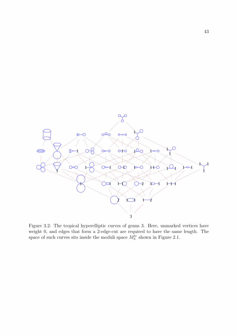
43

1 11

1

11111 11 1 1

11

1

1 1 2 1 111

1 1

1 1 1

1

1

1

2 11 21

3

Figure 3.2: The tropical hyperelliptic curves of genus 3. Here, unmarked vertices haveweight 0, and edges that form a 2-edge-cut are required to have the same length. Thespace of such curves sits inside the moduli space M tr

3 shown in Figure 2.1.

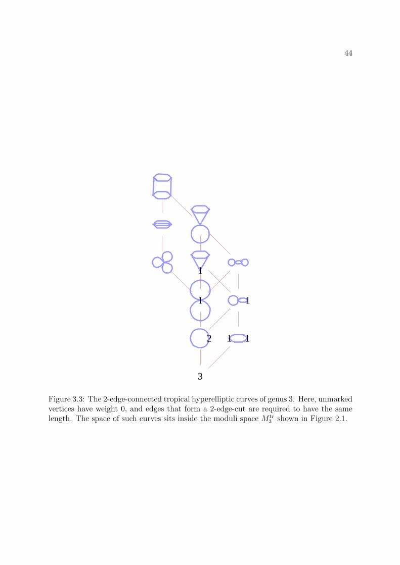
44

1

1 1

2 11

3

Figure 3.3: The 2-edge-connected tropical hyperelliptic curves of genus 3. Here, unmarkedvertices have weight 0, and edges that form a 2-edge-cut are required to have the samelength. The space of such curves sits inside the moduli space M tr

3 shown in Figure 2.1.

45

§3.2.2 Automorphisms and quotients

Let (G, l) be a loopless model for a metric graph Γ. An automorphism of (G, l) is aharmonic morphism φ : (G, l) → (G, l) of degree 1 such that the map V (G) ∪ E (G) →V (G) ∪ E (G) is a bijection. Equivalently, an automorphism of (G, l) is an automor-phism of G that also happens to preserve the length function l. The group of all suchautomorphisms is denoted Aut(G, l).

An automorphism of Γ is an isometry Γ → Γ. We assume throughout that Γ is nota circle, so the automorphisms Aut(Γ) of Γ form a finite group, since they permute thefinitely many points of Γ of valence 6= 2. Then automorphisms of Γ correspond preciselyto automorphisms of the canonical loopless model (G−, l) for Γ. An automorphism i isan involution if i2 = id.

Let (G, l) be a loopless model, and let K be a subgroup of Aut(G, l). We will nowdefine the quotient loopless model (G/K, l′). The vertices of G/K are the K-orbitsof V (G), and the edges of G/K are the K-orbits of those edges xy of G such that x andy lie in distinct K-orbits. If e ∈ E(G) is such an edge, let [e] ∈ E(G/K) denote the edgecorresponding to its K-orbit. The length function

l′ : E (G/K) → R>0

is given byl′ ([e]) = l (e) · | Stab(e)|

for every edge e ∈ E (G) with K-inequivalent ends. Notice that l′ is well-defined onE (G/K). Note also that (G/K, l′) is a loopless model.

Remark 3.2.1. If K is generated by an involution i on (G, l), then computing the lengthfunction l′ on the quotient G/K is very easy. By definition, edges of G in orbits of size 2have their length preserved, edges of G flipped by i are collapsed to a vertex, and edgesof G fixed by i are stretched by a factor of 2. See Figure 3.1.

The definition of the quotient metric graph follows the definition in [BN09] in the caseof nonmetric graphs, but has the seemingly strange property that edges can be stretchedby some integer factor in the quotient. The reason for the stretching is that it allows thenatural quotient morphism to be harmonic. Indeed, let (G, l) be a loopless model, letK be a subgroup of Aut(G, l), and let (G/K, l′) be the quotient. Define a morphism ofloopless models

πK : (G, l) → (G/K, l′)

as follows. If v ∈ V (G), let πK(v) = [v]. If e ∈ E(G) has K-equivalent ends x and y,then let πK(e) = [x] = [y]. If e ∈ E(G) has K-inequivalent ends, then let πK(e) = [e].

Lemma 3.2.2. Let (G, l) be a loopless model, let K be a subgroup of Aut(G, l), and let(G/K, l′) be the quotient. Then the quotient morphism πK : (G, l) → (G/K, l′) constructedabove is a harmonic morphism. If the graph G/K does not consist of a single vertex, thenπK is nondegenerate of degree |K|.

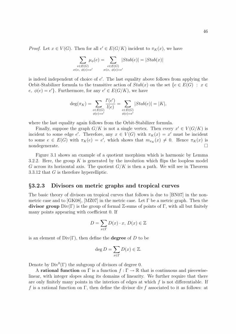
46

Proof. Let x ∈ V (G). Then for all e′ ∈ E(G/K) incident to πK(x), we have

∑


µφ(e) =∑


|Stab(e)| = |Stab(x)|

is indeed independent of choice of e′. The last equality above follows from applying theOrbit-Stabilizer formula to the transitive action of Stab(x) on the set {e ∈ E(G) : x ∈e, φ(e) = e′}. Furthermore, for any e′ ∈ E(G/K), we have

deg(πK) =∑

e∈E(G)φ(e)=e′

l′(e′)

l(e)=∑

e∈E(G)φ(e)=e′

|Stab(e)| = |K|,

where the last equality again follows from the Orbit-Stabilizer formula.Finally, suppose the graph G/K is not a single vertex. Then every x′ ∈ V (G/K) is

incident to some edge e′. Therefore, any x ∈ V (G) with πK(x) = x′ must be incidentto some e ∈ E(G) with πK(e) = e′, which shows that mπK

(x) 6= 0. Hence πK(x) isnondegenerate.

Figure 3.1 shows an example of a quotient morphism which is harmonic by Lemma3.2.2. Here, the group K is generated by the involution which flips the loopless modelG across its horizontal axis. The quotient G/K is then a path. We will see in Theorem3.3.12 that G is therefore hyperelliptic.

§3.2.3 Divisors on metric graphs and tropical curves

The basic theory of divisors on tropical curves that follows is due to [BN07] in the non-metric case and to [GK08], [MZ07] in the metric case. Let Γ be a metric graph. Then thedivisor group Div(Γ) is the group of formal Z-sums of points of Γ, with all but finitelymany points appearing with coefficient 0. If

D =∑

x∈Γ

D(x) · x, D(x) ∈ Z

is an element of Div(Γ), then define the degree of D to be

degD =∑

x∈Γ

D(x) ∈ Z.

Denote by Div0(Γ) the subgroup of divisors of degree 0.A rational function on Γ is a function f : Γ → R that is continuous and piecewise-

linear, with integer slopes along its domains of linearity. We further require that thereare only finitely many points in the interiors of edges at which f is not differentiable. Iff is a rational function on Γ, then define the divisor div f associated to it as follows: at

47

any given point x ∈ Γ, let (div f)(x) be the sum of all slopes that f takes on along edgesemanating from x.

The group of principal divisors is defined to be

Prin(Γ) = {div f : f a rational function on Γ}.

One may check that Prin(Γ) ⊆ Div0(Γ). Then the Jacobian Jac(Γ) is defined to be

Jac(Γ) =Div0(Γ)

Prin(Γ).

Note that Jac(Γ) = 1 if and only if Γ is a tree; this follows from [BF11, Corollary 3.3].A divisor D ∈ Div(Γ) is effective, and we write D ≥ 0, if D =

∑x∈ΓD(x) · x with

D(x) ∈ Z≥0 for all x ∈ X. We say that two divisors D and D′ are linearly equivalent,and we write D ∼ D′, if D−D′ ∈ Prin(Γ). Then the rank of a divisor D is defined to be

max{k ∈ Z : for all E ≥ 0 of degree k, there exists E ′ ≥ 0 such that D − E ∼ E ′ }.

Note that a divisor not equivalent to any effective divisor thus has rank −1.

Definition 3.2.3. A metric graph is hyperelliptic if it has a divisor of degree 2 andrank 1.

Let us extend the above definition to abstract tropical curves. The definition we willgive is due to [ABC11]. First, we recall:

Definition 3.2.4. An abstract tropical curve is a triple (G,w, l), where (G, l) is amodel for a metric graph Γ, and

w : V (G) → Z≥0

is a weight function satisfying a stability condition as follows: every vertex v with w(v) = 0has valence at least 3.

Now given a tropical curve (G,w, l) with underlying metric graph Γ, let Γw be themetric graph obtained from Γ by adding at each vertex v ∈ V (G) a total of w(v) loopsof any lengths.

Definition 3.2.5. An abstract tropical curve (G,w, l) with underlying metric graph Γ ishyperelliptic if Γw is hyperelliptic, that is, if Γw admits a divisor of degree 2 and rank 1.

Remark 3.2.6. We will see in Theorem 3.3.12 that the definition of hyperellipticity doesnot depend on the lengths of the loops that we added to Γ.

48

§3.2.4 Pullbacks of divisors and rational functions

Let φ : Γ → Γ′ be a harmonic morphism, and let g : Γ′ → R be a rational function. Thepullback of g is the function φ∗g : Γ → R defined by

φ∗g = g ◦ φ.

One may check that φ∗g is again a rational function. The pullback map on divisors

φ∗ : Div Γ′ → Div Γ

is defined as follows: given D′ ∈ Div Γ′, let

(φ∗ (D′)) (x) = mφ (x) ·D′ (φ(x))

for all x ∈ Γ. The following extends [BN09, Proposition 4.2(ii)] to metric graphs. It willbe used in the proof of Theorem 3.3.2.

Proposition 3.2.7. Let φ : Γ → Γ′ be a harmonic morphism of metric graphs, and letg : Γ′ → R be a rational function. Then

φ∗ div g = div φ∗g.

Remark 3.2.8. The two occurrences of φ∗ are really different operations, one on divisorsand the other on rational functions. Also, note that there is an analogous statementfor pushforwards along φ, as well as many other analogues of standard properties ofholomorphic maps, but we do not need them here.

Proof. It is straightforward (and we omit the details) to show that we may break Γand Γ′ into sets S and S ′ of segments along which φ∗g and g, respectively, are linear,and furthermore, such that each segment s ∈ S is mapped linearly to some s′ ∈ S ′ orcollapsed to a point. Then at any point x′ ∈ Γ, we have

(div g)(x′) =∑

s′=x′y′∈S′

g(y′) − g(x′)

l(s′).

So for any x ∈ Γ,

(φ∗ div g)(x) = mφ(x)∑

s′=φ(x)y′∈S′

g(y′) − g(φ(x))

l(s′)

=∑


∑

s=xy∈φ−1(s′)

l(s′)

l(s)·g(y′) − g(φ(x))

l(s′)

=∑


∑

s=xy∈φ−1(s′)

g(φ(y)) − g(φ(x))

l(s)

= (div φ∗g)(x).

49

3.3 When is a metric graph hyperelliptic?

Our goal in this section is to prove Theorem 3.3.12, which characterizes when a metricgraph hyperelliptic. It is the metric analogue of one of the main theorems of [BN09].We will first prove the theorem for 2-edge-connected metric graphs in Theorem 3.3.2 andthen prove the general case.

Given f a rational function on a metric graph Γ, let M (f) (respectively m (f)) denotethe set of points of Γ at which f is maximized (respectively minimized). Recall that agraph is said to be k-edge-connected if removing any set of at most k − 1 edges fromit yields a connected graph. A metric graph Γ is said to be k-edge-connected if theunderlying graph G0 of its canonical model (G0, l) is k-edge-connected. Thus a metricgraph is 2-edge-connected if and only if any model for it is 2-edge-connected, althoughthe analogous statement is false for k > 2.

The next lemma studies the structure of tropical rational functions with precisely twozeroes and two poles. It is important to our study of hyperelliptic curves because if Γ isa graph with a degree two harmonic morphism φ to a tree T and D = y − x ∈ PrinT ,then the pullback φ∗(D) is a principal divisor on Γ with two zeroes and two poles byProposition 3.2.7.

Lemma 3.3.1. Let Γ be a 2-edge connected metric graph; let f be a rational function onΓ such that

div f = y + y′ − x− x′

for x, x′, y, y′ ∈ Γ such that the sets {x, x′} and {y, y′} are disjoint. Then

(i) ∂M(f) = {x, x′} and ∂m(f) = {y, y′}, where ∂ denotes the boundary. In fact,there are precisely two edges leaving M(f), one at x and one at x′, and preciselytwo edges leaving m(f), one at y and one at y′. Furthermore, there is an x−x′ pathin M(f), and a y−y′ path in m(f).

(ii) f never takes on slope greater than 1. Furthermore, for any w ∈ Γ, let s+(w),(resp. s−(w)) denote the total positive (resp. negative) outgoing slope from w. Then

s+(w) ≤ 2 and s−(w) ≥ −2.

(iii) Given w ∈ Γ with (div f)(w) = 0, the multiset of outgoing nonzero slopes at w is ∅,{1,−1}, or {1, 1,−1,−1}.

Proof. Let D = div f . Note that D < 0 at any point in ∂M(f), so ∂M(f) ⊂ {x, x′}.Now, ∂M(f) must be nonempty since div f 6= 0. If |∂M(f)| = 1, then since M(f) has atleast two edges leaving it (since Γ is 2-edge-connected), and f is decreasing along them,then we must have x = x′ and ∂M(f) = {x} as desired. Otherwise, |∂M(f)| = 2 andagain ∂M(f) = {x, x′}. Now, f must decrease along any segment leaving M(f), andthere are at least two such segments by 2-edge-connectivity of Γ. By inspecting D, weconclude that there exactly two such segments, one at x and one at x′. Furthermore,

50

suppose x 6= x′. Then deleting the segment leaving M(f) at x cannot separate x fromm(f), again by 2-edge-connectivity, so there is an x−x′ path in M(f). The analogousresults hold for m(f). This proves (i).

Let us prove (ii). Pick any w ∈ Γ. We will show that s+(w) ≤ 2, and moreover, that ifs+(w) = 2 then there are precisely two directions at w along which f has outgoing slope+1. An analogous argument holds for s−(w), so (ii) will follow.

Let U be the union of all paths in Γ that start at w and along which f is nonincreasing.Let w1, . . . , wl be the set of points in U that are either vertices of Γ or are points at whichf is not differentiable. Let W = {w,w1, . . . , wl}. Then U\W consists of finitely manyopen segments. Let S = {s1, . . . , sk} be the set of closures of these segments. So theclosed segments s1, . . . , sk cover U and intersect at points in W , and f is linear alongeach of them. Orient each segment in S for reference, and for each y ∈W , let

δ+(y) = {j : sj is outgoing at y},

δ−(y) = {j : sj is incoming at y}.

Finally, for each i = 1, . . . , k, let mi ∈ Z be the slope that f takes on along the (oriented)segment si.

The key observation regarding U is that the slope of f along any edge e leaving Umust be positive, because otherwise e would lie in U . Therefore we have

D(wi) ≥∑

j∈δ+(wi)

mj −∑

j∈δ−(wi)

mj for i = 1, . . . , l, (3.1)

D(w) ≥∑

j∈δ+(w)

mj −∑

j∈δ−(w)

mj − s+(w). (3.2)

Summing (3.1) and (3.2), we have

D(w) +D(w1) + · · · +D(wl) ≥ s+(w). (3.3)

Since D = y + y′ − x− x′, we must have s+(w) ≤ 2.Suppose s+(w) = 2. Then the inequality (3.3) must be an equality, and so (3.1) and

(3.2) must also be equalities. In particular, no segment leaves U except at w. Since Γ is2-edge-connected and ∂U = {w}, it follows that there are precisely two directions at walong which f has outgoing slope +1. This proves (ii).

Finally, part (iii) follows directly from (ii).

We now come to the metric version of [BN09, Theorem 5.12], which gives equivalentcharacterizations of hyperellipticity for 2-edge-connected metric graphs.

Theorem 3.3.2. Let Γ be a 2-edge-connected metric graph, and let (G, l) denote itscanonical loopless model. Then the following are equivalent:



51

(iii) There exists a nondegenerate harmonic morphism of degree 2 from G to a tree, or|V (G)| = 2.

Proof. First, if |V (G)| = 2, then G must be the unique graph on 2 vertices and n edges,and so all three conditions hold. So suppose |V (G)| > 2. Let us prove (i) ⇒ (ii).

Let D ∈ Div Γ be a divisor of degree 2 and rank 1. We will now define an involutioni : Γ → Γ and then show that it induces an involution i : G→ G on its model. By slightabuse of notation, we will call both of these involutions i. We will then prove that G/i isa tree.

We define i : Γ → Γ as follows. Given x ∈ Γ, since D has rank 1, there exists x′ ∈ Γsuch that D ∼ x+ x′. Since Γ is 2-edge-connected, this x′ is unique. Then let i(x) = x′.Clearly i is an involution on sets.

Claim 3.3.3. The map i : Γ → Γ is an isometry.

Proof of Claim 3.3.3. Let x, y ∈ Γ, and let x′ = i(x), y′ = i(y). We will show that

d(x, y) = d(x′, y′)

with respect to the shortest path metric on Γ. We may assume x 6= y and x 6= y′, forotherwise the statement is clear.

By construction, we have x + x′ ∼ y + y′, so let f : Γ → R be a rational function onΓ such that

div f = y + y′ − x− x′.

By Lemma 3.3.1(i), we have ∂M(f) = {x, x′} and ∂m(f) = {y, y′}. Furthermore, M(f)has precisely two edges leaving it, one at x and one at x′. Similarly, m(f) has preciselytwo edges leaving it, one at y and one at y′.

By a path down from x we mean a path in Γ that starts at x and along which f isdecreasing, and which is as long as possible given these conditions. By Lemma 3.3.1(ii),f must have constant slope −1 along such a path. Furthermore, by Lemma 3.3.1(iii),any path down from x must end at y or y′. After all, if it ended at some point w withdiv f(w) = 0, then it would not be longest possible. Similarly, every path down from x′

must end at y or y′.So let P be a path down from x, and let l be its length in Γ. Suppose that P ends at

y. Note that d(x, y) = l. Indeed if there were a shorter path from x to y, then f wouldhave an average slope of less than −1 along it, contradicting Lemma 3.3.1(ii). Also, byLemma 3.3.1(iii), there must exist a path P ′ down from x′ to m(f) that is edge-disjointfrom P , so P ′ must end at y′. Now, P and P ′ have the same length since f decreasesfrom its maximum to its minimum value at constant slope −1 along each of them. Thusd(x′, y′) = l, and d(x, y) = d(x′, y′) as desired.

So we may assume instead that every path P down from x ends at y′. Then every pathdown from x′ must end at y, and no pair of x–y′ and x–y paths has a common vertex,for otherwise we could find a path down from x that ends at y. Thus x 6= x′ and y 6= y′

and, by Lemma 3.3.1, there is in fact a unique path Pxy′ down from x ending at y′ and

52

a unique path Px′y down from x′ ending at y. Then Pxy′ and Px′y have the same length,say l, by the argument above. Let δ be the length of a shortest path S in Γ between Pxy′and Px′y, and note that f must be constant on S. Then

d(x, y) = δ + l = d(x′, y′),

proving the claim.

Thus the involution i : Γ → Γ induces an automorphism i : G → G of canonicalloopless models. Then by Lemma 3.2.2, it induces a quotient morphism

π : G→ G/i

which is a nondegenerate harmonic morphism of degree two. In particular, we note thatG/i does not consist of a single vertex, since G had more than two vertices by assumption.

The final task is to show that G/i is a tree. In [BN09], this is done by by showingthat Jac (G/i) = 1 using the pullback of Jacobians along harmonic morphisms. Here,we will instead prove directly, in several steps, that the removal of any edge e from G/idisconnects it. If so, then G/i is necessarily a tree.

Claim 3.3.4. Let e ∈ E(G/i). Then π−1(e) consists of two edges.

Proof of Claim 3.3.4. Suppose instead that π−1(e) consists of a single edge e = xy ∈E (G). Then i fixes e, and i(x) = x and i(y) = y. Regarding e as a segment of Γ, choosepoints x0, y0 in the interior of e such that the subsegment x0y0 of e has length < d (x, y).Then i(x0) = x0 and i(y0) = y0, so D ∼ 2x0 ∼ 2y0. So there exists f : G → R withdiv f = 2x0 − 2y0. Then there are two paths down from x0 to y0, necessarily of the samelength in G; but one of them is the segment x0y0 and the other one passes through x andy, contradiction.

Claim 3.3.5. Let e ∈ E(G/i), and let π−1(e) = {e, e′}. Let e have vertices x, y and e′

have vertices x′, y′, labeled so that π(x) = π(x′) and π(y) = π(y′). Then in G \ {e, e′},there is no path from {x, x′} to {y, y′}.

Proof of Claim 3.3.5. By definition of the quotient map π, we have i(x) = x′ and i(y) =y′. Since x+ x′ ∼ y + y′, we may pick a rational function f on Γ such that

div f = y + y′ − x− x′.

Then f is linear along both e and e′. By Lemma 3.3.1(i), we have ∂M(f) = {x, x′}and ∂m(f) = {y, y′}, and by Lemma 3.3.1(ii), f must have constant slope 1 along eachof e and e′, decreasing from {x, x′} to {y, y′}. Then again by Lemma 3.3.1(i), e and e′

separate {x, x′} from {y, y′}.

Claim 3.3.6. Any edge e ∈ E(G/i) is a cut edge, that is, its removal disconnects G/i.

53

Proof of Claim 3.3.6. By Claim 3.3.4, we may let π−1(e) = {e, e′}. Let e have verticesx, y and e′ have vertices x′, y′, and let x = π(x) = π(x′) and y = π(y) = π(y′) be thevertices of e.

Suppose for a contradiction that there is a path in G/i from x to y not using e. Bynondegeneracy of π, we may lift that path to a path in G from x to y or y′ that does notuse e or e′. But this contradicts Claim 3.3.5.

We conclude that G/i is a tree. We have shown (i) implies (ii).(ii) ⇒ (iii). This is precisely Lemma 3.2.2.(iii) ⇒(i). This argument follows [BN09]. Let φ : (G, l) → (T, l′) be a nondegenerate

degree 2 harmonic morphism of loopless models, where T is a tree. Let φ : Γ → T be theinduced map on metric graphs, also denoted φ by abuse of notation. Pick any y0 ∈ Tand, regarding y0 as a divisor of degree 1, let D = φ∗(y0). So D is an effective divisoron Γ of degree 2, say D = y + y′. Now we have r(D) ≤ 1, for otherwise, for any z ∈ Γ,we would have (y + y′) − (z + y′) ∼ 0, so y ∼ z, so Γ itself would be a tree. It remainsto show r(D) ≥ 1. Let x ∈ Γ. Then φ(x) ∼ y0, since JacT = 1. Then by Proposition3.2.7, we have

D = φ∗(y0) ∼ φ∗(φ(x))

= mφ(x) · x+ E

for E an effective divisor on Γ. Since φ is nondegenerate, we havemφ(x) ≥ 1, soD ∼ x+E ′

for some effective E ′, as desired. This completes the proof of Theorem 3.3.2.

In the next section, we will use the fact that the hyperelliptic involution in Theo-rem 3.3.2(ii) is unique. To prove uniqueness, we need the following fact.

Proposition 3.3.7. [BN09, Proposition 5.5] If D and D′ are degree 2 divisors on ametric graph Γ with r(D) = r(D′) = 1, then D ∼ D′.

Proof. The proof of [BN09, Proposition 5.5] extends immediately to metric graphs.

Corollary 3.3.8. [BN09, Corollary 5.14] Let Γ be a 2-edge-connected hyperelliptic metricgraph. Then there is a unique involution i : Γ → Γ such that Γ/i is a tree.

Proof. Suppose i and i′ are two such involutions. From the proof of Theorem 3.3.2, wesee that for any x ∈ Γ, x + i(x) and x + i′(x) are both divisors of rank 1. Then byProposition 3.3.7, x + i(x) ∼ x + i′(x), so i(x) ∼ i′(x). Since Γ is 2-edge-connected, itfollows that i(x) = i′(x).

Our next goal is to prove Theorem 3.3.12, which extends Theorem 3.3.2 to graphswith bridges. Theorem 3.3.12 has no analogue in [BN09] because it takes advantage ofthe integer stretching factors present in morphisms of metric graphs which do not occurin combinatorial graphs.

Let us say that a point s in a metric graph Γ separates y, z ∈ Γ if every y–z path in Γpasses through s, or equivalently, if y and z lie in different connected components of Γ\s.A cut vertex is a point x ∈ Γ such that Γ \ x has more than one connected component.

54

Lemma 3.3.9. Let Γ be a 2-edge-connected hyperelliptic metric graph with hyperellipticinvolution i, and let x be a cut vertex of Γ. Then i(x) = x.

Proof. Suppose i(x) 6= x. Since x is a cut vertex, we may pick some y ∈ Γ such thatx separates y and i(x), so i(x) does not separate x and y. Furthermore, since i is anautomorphism, i(x) separates i(y) and x. Therefore i(x) separates y and i(y). ButLemma 3.3.1(i), applied to a rational function f with

div f = y + i(y) − x− i(x),

yields the existence of a y—i(y) path in m(f) not passing through i(x), contradiction.

Lemma 3.3.10. Let Γ be a metric graph, and let Γ′ be the metric graph obtained fromΓ by contracting all bridges. Let ϕ : Γ → Γ′ be the natural contraction morphism. GivenD ∈ Div Γ, let D′ ∈ Div Γ′ be given by

D′ =∑

x∈Γ

D(x) · ϕ(x).

Then D ∈ Prin Γ if and only if D′ ∈ Prin Γ′.

Proof. By induction, we may assume that Γ′ was obtained by contracting a single bridgee in Γ, and that D is not supported on the interior of e. Let e have endpoints x1 and x2,and for i = 1, 2, let Γi denote the connected component of xi in Γ \ e. Let Γ′

i = ϕ(Γi),and let x′ = ϕ(x1) = ϕ(x2) = ϕ(e).

Now suppose D ∈ Prin Γ, so let D = div f for f a rational function on Γ. Define f ′

on Γ as follows: let f ′(ϕ(y)) = f(y) for y ∈ Γ1, and f ′(ϕ(y)) = f(y) + f(x1) − f(x2)for y ∈ Γ2. This uniquely defines a rational function f ′ on Γ′, and one can check thatdiv f ′ = D′.

Conversely, suppose D′ = div f ′ ∈ Prin Γ′. Let

m = D(x1) −∑

outgoing slopes from x′ into Γ′1.

Now define f on Γ as follows: let f(x) = f ′(ϕ(x)) if x ∈ Γ1, let f(x) = f ′(ϕ(x)) +m · l(e)if x ∈ Γ2, and let f be linear with slope m along e. Then one can check that f is arational function on Γ with div f = D.

It follows from Lemma 3.3.10 that the rank of divisors is preserved under contractingbridges. The argument can be found in [BN09, Corollaries 5.10, 5.11], and we will notrepeat it here. In particular, we obtain

Corollary 3.3.11. Let Γ be a metric graph, and let Γ′ be the metric graph obtained fromΓ by contracting all bridges. Then Γ is hyperelliptic if and only if Γ′ is hyperelliptic.

We can finally prove the main theorem of the section, which generalizes Theorem3.3.2.

55

Theorem 3.3.12. Let Γ be a metric graph with no points of valence 1, and let (G, l)denote its canonical loopless model. Then the following are equivalent:



(iii) There exists a nondegenerate harmonic morphism of degree 2 from G to a tree, or|V (G)| = 2.

Proof. As in the proof of Theorem 3.3.2, we may assume that |V (G)| > 2. In fact, theproofs of (ii) ⇒ (iii) and (iii) ⇒ (i) from Theorem 3.3.2 still hold here, since they do notrely on 2-edge-connectivity. We need only show (i) ⇒ (ii).

Let Γ be a hyperelliptic metric graph with no points of valence 1, and let Γ′ be obtainedby contracting all bridges of Γ. Then Γ′ is hyperelliptic by Corollary 3.3.11. Since Γ hadno points of valence 1, the image of any bridge in Γ is a cut vertex x ∈ Γ′. By Lemma3.3.9, all such vertices are fixed by the hyperelliptic involution i′ on Γ′. Thus, we canextend i′ uniquely to an involution i on Γ by fixing, pointwise, each bridge of Γ. Theni is also an involution on the canonical loopless model (G, l), and G/i is a tree whosecontraction by the images of the bridges of G is the tree Γ′/i′.

Remark 3.3.13. The requirement that Γ has no points of valence 1 is not important,because Corollary 3.3.11 allows us to contract such points away. Also, because of Defini-tion 3.2.5 and the stability condition on tropical curves, we will actually never encounterpoints of valence 1 in the tropical context.

3.4 The hyperelliptic locus in tropical Mg

Which tropical curves of genus g are hyperelliptic? In this section, we will use the maincombinatorial tool we have developed, Theorem 3.3.12, to construct the hyperellipticlocus Htr

g in the moduli space M trg of tropical curves. The space M tr

g was defined in[BMV11] and computed explicitly for g ≤ 5 in [Cha11a]. It is (3g − 3)-dimensional andhas the structure of a stacky fan, as defined in Definition 2.3.2.

It is a well-known fact that the classical hyperelliptic locus Hg ⊂ Mg has dimension2g−1. Therefore, it is surprising that Htr

g is actually (3g−3)-dimensional, as observed in[LPP11], especially given that tropicalization is a dimension-preserving operation in manyimportant cases [BG84]. However, if one considers only 2-edge-connected tropical curves,

then the resulting locus, denotedH(2),trg , is in fact (2g−1)-dimensional. The combinatorics

of H(2),trg is nice, too: in Theorem 3.4.9 we prove that the (2g − 1)-dimensional cells are

graphs that we call ladders of genus g. See Definition 3.4.7 and Figure 3.6. We thenexplicitly compute the spaces Htr

3 , H(2),tr3 and H

(2),tr4 .

56

§3.4.1 Construction of Htrg

and H(2),trg

We will start by giving a general framework for constructing parameter spaces of tropicalcurves in which edges may be required to have the same length. We will see that theloci Htr

g and H(2),trg of hyperelliptic and 2-edge-connected hyperelliptic tropical curves,

respectively, fit into this framework.Recall that a combinatorial type of a tropical curve is a pair (G,w), where G is a

connected, non-metric multigraph, possibly with loops, and w : V (G) → Z≥0 satisfies thestability condition that if w(v) = 0 then v has valence at least 3. The genus of (G,w) is

|E(G)| − |V (G)| + 1 +∑

v∈V (G)

w(v).

Now, a constrained type is a triple (G,w, r), where (G,w) is a combinatorial typeand r is an equivalence relation on the edges of G. We regard r as imposing the constraintthat edges in the same equivalence class must have the same length. Given a constrainedtype (G,w, r) and a union of equivalence classes S = {e1, . . . , ek} of r, define the con-traction along S as the constrained type (G′, w′, r′). Here, (G′, w′) is the combinatorialtype obtained by contracting all edges in S. Contracting a loop, say at vertex v, meansdeleting it and adding 1 to w(v). Contracting a nonloop edge, say with endpoints v1

and v2, means deleting that edge and identifying v1 and v2 to obtain a new vertex whoseweight is w(v1) + w(v2). Finally, r′ is the restriction of r to E(G) \ S.

An automorphism of (G,w, r) is an automorphism ϕ of the graph G which is compat-ible with both w and r. Thus, for every vertex v ∈ V (G), we have w(ϕ(v)) = w(v), andfor every pair of edges e1, e2 ∈ E(G), we have that e1 ∼r e2 if and only if ϕ(e1) ∼r ϕ(e2).Let Nr denote the set of equivalence classes of r. Note that the group of automorphismsAut(G,w, r) acts naturally on the set Nr, and hence on the orthant RNr

≥0, with the lat-

ter action given by permuting coordinates. We define C(G,w, r) to be the topologicalquotient space

C(G,w, r) =RNr

≥0

Aut(G,w, r).

Now, suppose C is a collection of constrained types that is closed under contraction.Define an equivalence relation ∼ on the points in the union

∐

(G,w,r)∈C

C(G,w, r)

as follows. Regard a point x ∈ C(G,w, r) as an assignment of lengths to the edges of Gsuch that r-equivalent edges have the same length. Given two points x ∈ C(G,w, r) andx′ ∈ C(G′, w′, r′), let x ∼ x′ if the two tropical curves obtained by contracting all edgesof length zero are isomorphic.

Now define the topological space MC as

MC =∐

C(G,w, r)/ ∼,

57

where the disjoint union ranges over all types (G,w, r) ∈ C. Since C is closed undercontraction, it follows that the points ofMC are in bijection with r-compatible assignmentsof positive lengths to E(G) for some (G,w, r) ∈ C.

Theorem 3.4.1. Let C be a collection of constrained types, as defined above, that is closedunder contraction. Then the space MC is a stacky fan, with cells corresponding to types(G,w, r) in C.

Proof. For the definition of a stacky fan, see Definition 2.3.2. The proof of Theorem 3.4.1is entirely analogous to the proof that the moduli space of genus g tropical curves is astacky fan, so we refer the reader to Theorem 2.3.4.

Remark 3.4.2. Note that the stacky fan MC is not in general a stacky subfan of M trg .

Instead, it may include only parts of the cells of M trg , since edges may be required to have

equal length.

Our next goal is to define the collections Cg and C2g of hyperelliptic and 2-edge-

connected hyperelliptic types of genus g. If (G,w) is a combinatorial type, let Gw

denote the graph obtained from G by adding w(v) loops at each vertex v. Let Gw−

be the loopless graph obtained by adding a vertex to the interior of each loop in Gw.Now let G and G′ be loopless graphs. Then a morphism φ : G → G′ is a map of setsV (G) ∪ E (G)→V (G′) ∪ E (G′) such that

(i) φ(V (G)) ⊆ V (G′),

(ii) if e = xy is an edge of G and φ (e) ∈ V (G′) then φ (x) = φ (e) = φ (y), and

(iii) if e = xy is an edge of G and φ(e) ∈ E (G′) then φ(e) is an edge between φ(x) andφ(y).

The morphism φ is harmonic if the map φ : (G,1) → (G′,1) of loopless models is aharmonic morphism, where 1 denotes the function assigning length 1 to every edge. Thedefinitions above follow [BN09].

Definition 3.4.3. A constrained type (G,w, r) is 2-edge-connected hyperelliptic if

(i) G is 2-edge-connected,

(ii) the loopless graph Gw− has a nondegenerate harmonic morphism φ of degree 2 to a

tree, or |V (G)| = 2, and

(iii) the relation r is induced by the fibers of φ on nonloop edges of G, and is trivial onthe loops of G.

The type (G,w, r) is said to be hyperelliptic if r is the trivial relation on bridges andthe type (G′, w′, r′) obtained by contracting all bridges is 2-edge-connected hyperellipticin the sense we have just defined.

58

Let Cg denote the collection of hyperelliptic types of genus g, and C(2)g the collection

of 2-hyperelliptic types of genus g.

Proposition 3.4.4. The collections Cg and C2g of hyperelliptic and 2-edge-connected hy-

perelliptic types defined above are closed under contraction.

Proof. We will check that C(2)g is closed under contraction. If so, then Cg is too, since

it was defined precisely according to contractions to types in C(2)g . Note also that by

definition, contraction preserves the genus g, whether the contracted edge was a loop ora nonloop edge.

Let (G,w, r) be a 2-hyperelliptic type, and let

ϕ : Gw− → T

be the unique harmonic morphism to a tree T that is either nondegenerate of degree 2,or T has 1 vertex and Gw

− has 2 vertices. Let S be a class of the relation r. Then thereare three cases: either S = {e} and e is a loop; or S = {e}, e is a nonloop edge, andϕ(e) ∈ V (T ); or S = {e1, e2} and ϕ(e1) = ϕ(e2) is an edge of T .

Suppose S = {e} and e is a loop. Then the contraction of (G,w, r) by e is (G/e, w′,r|E(G/e)), where w′ is obtained from w by adding 1 at v. Then

(G/e)w′

− = Gw−

so the same morphism ϕ shows that (G/e, w′, r|E(G/e)) is a 2-hyperelliptic type.Suppose S = {e}, e is a nonloop edge, and, regarding e as an edge of Gw

−, we haveϕ(e) = v ∈ V (T ). Let k be the number of edges in G that are parallel to e, and let T ′ bethe tree obtained from T by adding k leaves at v. Then we may construct a morphism

ϕ′ : (G/e)w′

− → T ′

which in particular sends the k edges parallel to e to the k new leaf edges of T ′, andwhich has the required properties. See Figure 3.4.

Suppose S = {e1, e2} where e1 and e2 are nonloop edges of G and ϕ(e1) = ϕ(e2) =e ∈ E(T ). Now, contracting {e1, e2} in Gw

− may create new loops, say k of them, asillustrated in Figure 3.5. Let T ′ be the tree obtained from T by adding k leaves at eitherend of the edge e and then contracting e. Then we may construct a harmonic morphism

ϕ′ : (G/{e1, e2})w− → T ′

which sends the k new loops to the k new leaves of T ′, and which has the requiredproperties.

Definition 3.4.5. The space Htrg of tropical hyperelliptic curves of genus g is defined to

be the space MCg, where Cg is the collection of hyperelliptic combinatorial types of genus

g defined above.The space H

(2),trg of 2-edge-connected tropical hyperelliptic curves of genus g is de-

fined to be the space MC(2)g

, where C(2)g is the collection of 2-edge-connected hyperelliptic

combinatorial types of genus g defined above.

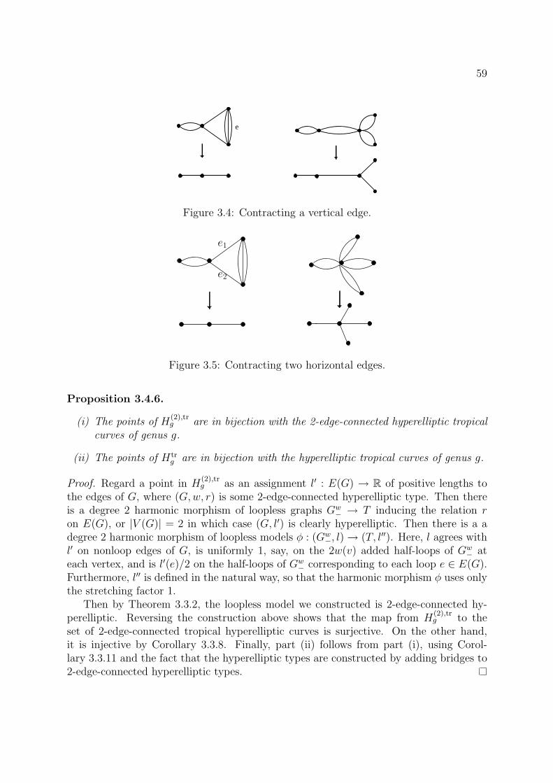
59

e

Figure 3.4: Contracting a vertical edge.

e1

e2

Figure 3.5: Contracting two horizontal edges.

Proposition 3.4.6.

(i) The points of H(2),trg are in bijection with the 2-edge-connected hyperelliptic tropical

curves of genus g.

(ii) The points of Htrg are in bijection with the hyperelliptic tropical curves of genus g.

Proof. Regard a point in H(2),trg as an assignment l′ : E(G) → R of positive lengths to

the edges of G, where (G,w, r) is some 2-edge-connected hyperelliptic type. Then thereis a degree 2 harmonic morphism of loopless graphs Gw

− → T inducing the relation ron E(G), or |V (G)| = 2 in which case (G, l′) is clearly hyperelliptic. Then there is a adegree 2 harmonic morphism of loopless models φ : (Gw

−, l) → (T, l′′). Here, l agrees withl′ on nonloop edges of G, is uniformly 1, say, on the 2w(v) added half-loops of Gw

− ateach vertex, and is l′(e)/2 on the half-loops of Gw

− corresponding to each loop e ∈ E(G).Furthermore, l′′ is defined in the natural way, so that the harmonic morphism φ uses onlythe stretching factor 1.

Then by Theorem 3.3.2, the loopless model we constructed is 2-edge-connected hy-perelliptic. Reversing the construction above shows that the map from H

(2),trg to the

set of 2-edge-connected tropical hyperelliptic curves is surjective. On the other hand,it is injective by Corollary 3.3.8. Finally, part (ii) follows from part (i), using Corol-lary 3.3.11 and the fact that the hyperelliptic types are constructed by adding bridges to2-edge-connected hyperelliptic types.

60

��

��

��

��

��

��

��

��

��

��

��

��

��

��

��

��

��

��

��

��

��

��

��

��

��

��

��

��

��

��

��

��

��

��

��

��

��

��

��

��

��

Figure 3.6: The ladders of genus 3, 4, and 5.

§3.4.2 Maximal cells of H(2),trg

Now we will prove that H(2),trg is pure of dimension 2g − 1, and we will characterize its

maximal cells. Recall that the dimension of a cell of the form RN≥0/G is equal to N , and

the dimension of a stacky fan is the largest dimension of one of its cells. It is pure if allof its maximal cells have the same dimension.

First, we define the graphs which, as it turns out, correspond to the maximal cells ofH

(2),trg .

Definition 3.4.7. Let T be any nontrivial tree with maximum valence ≤ 3. Constructa graph L(T ) as follows. Take two disjoint copies of T , say with vertex sets {v1, . . . , vn}and {v′1, . . . , v

′n}, ordered such that vi and v′i correspond. Now, for each i = 1, . . . , n,

consider the degree d = deg vi = deg v′i. If d = 1, add two edges between vi and v′i. Ifd = 2, add one edge between vi and v′i. The resulting graph L(T ) is a loopless connectedgraph, and by construction, every vertex has valence 3. We call a graph of the form L(T )for some tree T a ladder. See Figure 3.6.

Lemma 3.4.8. Let T be a tree on n vertices with maximum degree at most 3. Then thegenus of the graph L(T ) is n+ 1.

Proof. For i = 1, 2, 3, let ni denote the number of vertices in T of degree i. Then L(T )has 2n vertices and 2(n− 1) + 2n1 + n2 edges; hence its genus is g = 2n1 + n2 − 1. Also,double-counting vertex-edge incidences in T gives 2(n− 1) = n1 + 2n2 + 3n3. Adding, wehave

g + 2(n− 1) = 3n1 + 3n2 + 3n3 − 1 = 3n− 1,

so g = n+ 1.

Theorem 3.4.9. Fix g ≥ 3. The space H(2),trg of 2-edge-connected hyperelliptic tropical

curves of genus g is a stacky fan which is pure of dimension 2g − 1. The maximal cellscorrespond to ladders of genus g.

Remark 3.4.10. Note that the stacky fan H(2),trg is naturally a closed subset of M tr

g ,but it is not a stacky subfan because sometimes edges are required to have equal lengths.So its stacky fan structure is more refined than that of M tr

g . Compare Figure 3.3 andFigure 2.1.

61

Proof. Let (G,w, r) ∈ C(2)g be the type of a maximal cell in H

(2),trg . Our goal is to show

that w ≡ 0, that G = L(T ) for some tree T , and that r is the relation on E(G) inducedby the natural harmonic morphism

ϕT : L(T ) → T

of degree 2.First, we observe that the dimension of the cell C(G,w, r) is, by construction, the

number of equivalence classes of r. Now, we have, by definition of C(2)g , a morphism

ϕ : Gw− → T

where either Gw− has 2 vertices and T is trivial, or T is nontrivial and ϕ is a nondegenerate

harmonic morphism of degree 2.We immediately see that w is uniformly zero, for otherwise the cell C(Gw, 0, r′) would

contain C(G,w, r), contradicting maximality of the latter. Here, r′ denotes the relationon E(Gw) that is r on E(G) and trivial on the added loops of Gw.

Let us also dispense with the special case that G− has 2 vertices: if so, then G is theunique graph consisting of g + 1 parallel edges. But then our cell C(G, 0, r) is far frommaximal; in fact, it is contained in each cell corresponding to a ladder.

Therefore we may assume that T is nontrivial and ϕ : G− → T is a nondegeneratedegree 2 harmonic morphism.

Next, we claim that every vertex v ∈ V (G−) has horizontal multiplicity mϕ(v) = 1.This claim shows in particular that G has no loops. In fact, the intuition behind theclaim is simple: if mϕ(v) = 2, then split v into two adjacent vertices v′ and v′′ withϕ(v′) = ϕ(v′′) to make a larger cell. However, because G might a priori contain loops andthus G− might have vertices of degree 2, we will need to prove the claim carefully. Theproof is illustrated in Figure 3.7.

To prove the claim, suppose v ∈ V (G−) is such that mϕ(v) = 2. Let us assume thatdeg(v) > 2, i.e. that v is not the midpoint of some loop l of G, for if it is, then pick thebasepoint of l instead. Let w = ϕ(v). Let e1, . . . , ek ∈ E(T ) be the edges of T incident tow, and let w1, . . . , wk denote their respective endpoints that are different from w. Now,for each i = 1, . . . , k, the set ϕ−1(ei) consists of two edges of G−; call them ai and bi. Byrenumbering them, we may assume that the first j of the pairs form loops in G. That is,if 1 ≤ i ≤ j, then the edges ai and bi have common endpoints vi and v, with deg(vi) = 2.

Let us construct a new graph G′ and relation r′ such that (G, 0, r) is a contractionof (G′, 0, r′). Replace the vertex v with two vertices, va and vb, where va is incident toedges a1, . . . , ak and vb is incident to edges b1, . . . , bk. Now suppress the degree 2 verticesv1, . . . , vj, so that for 1 ≤ i ≤ j, the pair of edges {ai, bi} becomes a single edge ei. Finally,add an edge e between va and vb. Call the resulting graph G′. See Figure 3.7.

By construction, the graph G′ is a stable, 2-edge-connected graph with G′/e = G andwith the same genus as G. Let T ′ be the tree obtained from T by deleting e1, . . . , ej.Then there is a natural degree 2 harmonic morphism

ϕ′ : G′− → T ′

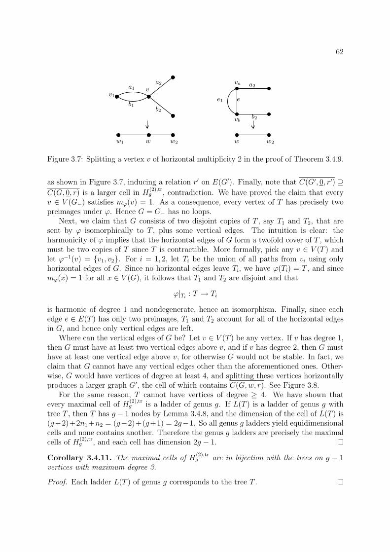
62

��

��

��

��

��

��

��

��

��

��

��

a2

b2

v1e1

w2 w2www1

a1

b1

va

e

vb

a2

b2

v

Figure 3.7: Splitting a vertex v of horizontal multiplicity 2 in the proof of Theorem 3.4.9.

as shown in Figure 3.7, inducing a relation r′ on E(G′). Finally, note that C(G′, 0, r′) ⊇

C(G, 0, r) is a larger cell in H(2),trg , contradiction. We have proved the claim that every

v ∈ V (G−) satisfies mϕ(v) = 1. As a consequence, every vertex of T has precisely twopreimages under ϕ. Hence G = G− has no loops.

Next, we claim that G consists of two disjoint copies of T , say T1 and T2, that aresent by ϕ isomorphically to T , plus some vertical edges. The intuition is clear: theharmonicity of ϕ implies that the horizontal edges of G form a twofold cover of T , whichmust be two copies of T since T is contractible. More formally, pick any v ∈ V (T ) andlet ϕ−1(v) = {v1, v2}. For i = 1, 2, let Ti be the union of all paths from vi using onlyhorizontal edges of G. Since no horizontal edges leave Ti, we have ϕ(Ti) = T , and sincemϕ(x) = 1 for all x ∈ V (G), it follows that T1 and T2 are disjoint and that

ϕ|Ti: T → Ti

is harmonic of degree 1 and nondegenerate, hence an isomorphism. Finally, since eachedge e ∈ E(T ) has only two preimages, T1 and T2 account for all of the horizontal edgesin G, and hence only vertical edges are left.

Where can the vertical edges of G be? Let v ∈ V (T ) be any vertex. If v has degree 1,then G must have at least two vertical edges above v, and if v has degree 2, then G musthave at least one vertical edge above v, for otherwise G would not be stable. In fact, weclaim that G cannot have any vertical edges other than the aforementioned ones. Other-wise, G would have vertices of degree at least 4, and splitting these vertices horizontallyproduces a larger graph G′, the cell of which contains C(G,w, r). See Figure 3.8.

For the same reason, T cannot have vertices of degree ≥ 4. We have shown thatevery maximal cell of H

(2),trg is a ladder of genus g. If L(T ) is a ladder of genus g with

tree T , then T has g − 1 nodes by Lemma 3.4.8, and the dimension of the cell of L(T ) is(g−2)+2n1 +n2 = (g−2)+(g+1) = 2g−1. So all genus g ladders yield equidimensionalcells and none contains another. Therefore the genus g ladders are precisely the maximalcells of H

(2),trg , and each cell has dimension 2g − 1.

Corollary 3.4.11. The maximal cells of H(2),trg are in bijection with the trees on g − 1

vertices with maximum degree 3.

Proof. Each ladder L(T ) of genus g corresponds to the tree T .

63

��

��

��

��

��

��

��

��

��

��

��

��

��

��

��

��

��

��

Figure 3.8: Horizontal splits in G above vertices in T of degrees 1, 2, and 3, respectively.

Corollary 3.4.12. Let g ≥ 3. The number of maximal cells of H(2),trg is equal to the

(g − 2)nd term of the sequence

1, 1, 2, 2, 4, 6, 11, 18, 37, 66, 135, 265, 552, 1132, 2410, 5098, . . .

Proof. This is sequence A000672 in [OEIS], which counts the number of trees of maximumdegree 3 on a given number of vertices. Cayley obtained the first twelve terms of thissequence in 1875 [Cay75]; see [RS99] for a generating function. See Figure 3.6 for theladders of genus 3,4, and 5, corresponding to the first three terms 1, 1, and 2 of thesequence.

Remark 3.4.13. As pointed out in [LPP11], the stacky fan Htrg is full-dimensional for

each g. Indeed, take any 3-valent tree with g leaves, and attach a loop at each leaf. Theresulting genus g graph indexes a cell of dimension 3g − 3. Thus it is more natural toconsider the sublocus H

(2),trg , at least from the point of view of dimension.

One can use Theorem 3.4.9 to computeH(2),trg andHtr

g , the latter by adding all possible

bridges to the cells of H(2),trg . We will explicitly compute H

(2),tr3 , Htr

3 , and H(2),tr4 next.

The space Htr4 is too large to compute by hand.

§3.4.3 Computations

We now apply Theorem 3.4.9 to explicitly compute the spaces H(2),tr3 , Htr

3 , and H(2),tr4 .

Theorem 3.4.14. The moduli space H(2),tr3 of 2-edge-connected tropical hyperelliptic

curves has 11 cells and f -vector(1, 2, 2, 3, 2, 1).


Proof. The space M tr3 was computed explicitly in Theorem 2.2.12. A poset of genus 3

combinatorial types is shown in Figure 2.1. Now use Theorem 3.4.9.

64

Theorem 3.4.15. The moduli space Htr3 of tropical typerelliptic curves has 36 cells and

f -vector(1, 3, 6, 11, 9, 5, 1).


Proof. Apply Theorem 3.4.14 and Lemma 3.3.10.

Theorem 3.4.16. The moduli space H(2),tr4 of 2-edge-connected tropical hyperelliptic

curves of genus 4 has 31 cells and f -vector

(1, 2, 5, 6, 7, 6, 3, 1).

Proof. The space M tr4 was computed explicitly in Theorem 2.2.12, so we can apply The-

orem 3.4.9 directly to it.

3.5 Berkovich skeletons and tropical plane curves

In this section, we are interested in hyperelliptic curves in the plane over a complete,nonarchimedean valuated field K. Every such curve X is given by a polynomial of theform

P = y2 + f(x)y + h(x)

for f, h ∈ K[x]. We suppose that the Newton polygon of P is the lattice triangle inR2 with vertices (0, 0), (2g + 2, 0), and (0, 2). We write ∆2g+2,2 for this triangle. Since∆2g+2,2 has g interior lattice points, the curve X has genus g. The main theorem in thissection, Theorem 3.5.3, says that under certain combinatorial conditions, the Berkovichskeleton of X is a ladder over the path Pg−1 on g− 1 vertices. The main tool is [BPR11,Corollary 6.27], which states that under nice conditions, an embedded tropical planecurve, equipped with a lattice length metric, faithfully represents the Berkovich skeletonof X.

Recall that an embedded tropical curve T ⊆ R2 can be regarded as a metric spacewith respect to lattice length. Indeed, if e is a 1-dimensional segment in T , then ithas a rational slope. Then a ray from the origin with the same slope meets some firstlattice point (p, q) ∈ Z2. Then the length of e in the metric space T is its Euclideanlength divided by

√p2 + q2. By a standard ladder of genus g, we mean the graph

L(T ) defined above for T a path on g − 1 vertices. We will denote this graph Lg. Figure3.6 shows the standard ladders of genus 3, 4, and 5, as well as a nonstandard ladder ofgenus 5.

In Theorem 3.5.3, we will consider unimodular triangulations of ∆2g+2,2 with bridgelessdual graph. Such triangulations contain a maximally triangulated trapezoid of height 1in their bottom half (see Figure 3.9), so we study height 1 trapezoids in the next lemma.

Lemma 3.5.1. Fix a, b, c, d ∈ Z with a < b and c < d, and let Q be the lattice polytopewith vertices (a, 0), (b, 0), (c, 1), and (d, 1). Then any unimodular triangulation of Q has

65

��

��

��

��

��

��

��

��

��

��

��

1

2

3

4

4

3

2

1

21

10

−100

Figure 3.9: On the left, a unimodular triangulation N of ∆2g+2,2 that happens to includethe edge {(0, 2), (1, 0)} but not the edge {(0, 2), (2g + 1, 0)}. On the right, the tropicalplane curve dual to N has a core (shown in thick edges) that is a standard genus 3 ladder.The numbers on the edges indicate their slopes. We have chosen g = 3 in this illustration.

N = b − a + d − c + 1 nonhorizontal edges w1, . . . , wN satisfying w1 = {(a, 0), (c, 1)},wN = {(b, 0), (d, 1)}, and for each i = 1, . . . , N − 1, if wi has the form {(x, 0), (y, 1)} forsome x, y ∈ Z, then

wi+1 = {(x+ 1, 0), (y, 1)} or wi+1 = {(x, 0), (y + 1, 1)}.

Thus there are(b−a+d−cb−a

)such triangulations.

Proof. The edge {(a, 0), (c, 1)} is contained in some unimodular triangle ∆, so either{(a + 1, 0), (c, 1)} or {(a, 0), (c + 1, 1)} must be present. Now induct, replacing Q byQ− ∆.

Definition 3.5.2. Let T ⊆ Rn be an embedded tropical curve with dimH1(T,R) > 0.We define the core of T to be the smallest subspace Y ⊆ T such that there exists adeformation retract from T to Y . See Figure 3.9.

Theorem 3.5.3. Let X ⊆ T2 be a plane hyperelliptic curve of genus g ≥ 3 over acomplete nonarchimedean valuated field K, defined by a polynomial of the form P =y2 + f(x)y + h(x). Let X be its smooth completion. Suppose the Newton complex of Pis a unimodular triangulation of the lattice triangle ∆2g+2,2, and suppose that the core

of TropX is bridgeless. Then the skeleton Σ of the Berkovich analytification Xan is astandard ladder of genus g whose opposite sides have equal length.

66

Proof. Let Σ′ denote the core of T = TropX, and let N denote the Newton complex off , to which T is dual. Note that the lattice triangle ∆2g+2,2 has precisely g interior latticepoints (1, 1), . . . , (g, 1). Now, we claim that N cannot have any edge from (0, 2) to anypoint on the x-axis such that this edge partitions the interior lattice points nontrivially.(For example, the edge {(0, 2), (3, 0)} cannot be in N). Indeed, if such an edge werepresent in N , then the edge in T dual to it would be a bridge in Σ′, contradiction. Thensince all the triangles incident to the interior lattice points are unimodular, it follows thateach edge

s1 = {(1, 1), (2, 1)}, . . . , sg−1 = {(g − 1, 1), (g, 1)}

is in N , and for the same reason, that each edge

{(0, 2), (1, 1)}, . . . , {(0, 2), (g, 1)}

is in N . For i = 1, . . . , g − 1, the 2-face of N above (respectively, below) si correspondsto a vertex of T ; call this vertex Vi (respectively Wi).

Now, either the edge {(0, 2), (1, 0)} is in N , or it is not. If it is, then unimodularityimplies that the edges {(0, 1), (1, 0)} and {(1, 1), (1, 0)} are also in N . If not, then uni-modularity again implies that {(0, 1), (1, 1)} is in N . Similarly, if {(0, 2), (2g + 1, 0)} isin N , then the edges {(g, 1), (2g + 1, 0)} and {(g − 1, 1), (2g + 1, 0)} are in N . In each ofthese cases, N contains a unimodular triangulation of the trapezoidal region with vertices

(a, 0), (b, 0), (1, 1), (g, 1)

where we take a = 0 or a = 1 according to whether the edge {(0, 2), (1, 0)} is in N , andsimilarly we take b = 2g+1 or b = 2g+2 according to whether the edge {(0, 2), (2g+1, 0)}is in N . For example, in Figure 3.9, we take a = 1 and b = 2g + 2.

In each case, we see that the dual graph to N is a standard ladder of genus g, withvertices V1, . . . , Vg−1,W1, . . . ,Wg−1. In particular, there are two paths in T from V1 toW1 not passing through any other Vi or Wi, and similarly, there are two paths from Vg−1

to Wg−1.Moreover, we claim that for each i = 1, . . . , g − 2, the lattice-lengths of the paths in

Σ′ between Vi and Vi+1 and between Wi and Wi+1 are equal. Indeed, for each i, writeVi = (Vi,1, Vi,2) and Wi = (Wi,1,Wi,2). Notice that Vi,1 = Wi,1 for each i, because eachsegment si ∈ N is horizontal so its dual in T is vertical. Furthermore, the path fromWi to Wi+1 in Σ′ consists of a union of segments of integer slopes, so their lattice-lengthdistance is the horizontal displacement Wi+1,1 −Wi,1. Similarly, the distance in Σ′ fromVi to Vi+1 is Vi+1,1 − Vi,1 = Wi+1,1 − Wi,1, as desired. So Σ′ is a standard ladder ofgenus g, with opposite sides of equal length. Finally, we apply [BPR11, Corollary 6.27] to

conclude that the tropicalization map on the Berkovich analytification Xan of X inducesan isometry of the Berkovich skeleton Σ of Xan onto Σ′. This completes the proof ofTheorem 3.5.3.

In the proof above, we gained a refined combinatorial understanding of the unimodulartriangulations of ∆2g+2,2, which we make explicit in the following corollary.

67

Corollary 3.5.4. Consider unimodular triangulations of ∆2g+2,2 whose dual complex con-tains a bridgeless connected subgraph of genus g. There are

(3g+3g+1

)such triangulations that

use neither the edge e1 = {(0, 2), (1, 0)} nor the edge e2 = {(0, 2), (2g + 1, 0)}, there are2 ·(3g+1g

)triangulations using one of e1 and e2, and there are

(3g−1g−1

)triangulations using

both e1 and e2.

Proof. Use the proof of Theorem 3.5.3, which characterizes precisely which triangulationscan occur, and Lemma 3.5.1.

68

Chapter 4

Elliptic curves in honeycomb form

The content of this chapter is the paper [CS12] joint with Bernd Sturmfels and hasbeen submitted to the Proceedings of the CIEM Workshop on tropical geometry. Theversion here incorporates only minor changes.

4.1 Introduction

Suppose K is a field with a nonarchimedean valuation val : K∗ → R, such as the rationalnumbers Q with their p-adic valuation for some prime p ≥ 5 or the rational functionsQ(t) with the t-adic valuation. Throughout, we shall assume that the residue field of Khas characteristic different from 2 and 3.

We consider a ternary cubic polynomial whose coefficients cijk lie in K:

f(x, y, z) = c300x3 + c210x

2y + c120xy2 + c030y

3 + c021y2z

+ c012yz2 + c003z

3 + c102xz2 + c201x

2z + c111xyz.(4.1)

Provided the discriminant of f(x, y, z) is non-zero, this cubic represents an elliptic curveE in the projective plane P2

K . The group GL(3, K) acts on the projective space P9K of

all cubics. The field of rational invariants under this action is generated by the familiarj-invariant, which we can write explicitly (with coefficients in Z) as

j(f) =a polynomial of degree 12 in the cijk having 1607 terms

a polynomial of degree 12 in the cijk having 2040 terms. (4.2)

The Weierstrass normal form of an elliptic curve can be obtained from f(x, y, z) byapplying a matrix in GL(3, K). From the perspective of tropical geometry, however, theWeierstrass form is too limiting: its tropicalization never has a cycle. One would ratherhave a model for plane cubics whose tropicalization looks like the graphs in Figures 4.1,4.3 and 4.5. If this holds then we say that f is in honeycomb form. Cubic curves inhoneycomb form are the central object of interest in this chapter.

Honeycomb curves of arbitrary degree were studied in [Spe05a, §5]; they are dual tothe standard triangulation of the Newton polygon of f . For cubics in honeycomb form,

69

Figure 4.1: Tropicalizations of plane cubic curves in honeycomb form. The curve on theright is in symmetric honeycomb form; the one on the left is not symmetric.

by [KMM08], the lattice length of the hexagon equals −val(j(f)). Moreover, by [BPR11],a honeycomb cubic faithfully represents a subgraph of the Berkovich curve Ean.

A standard Newton subdivision argument [MS10] shows that a cubic f is in honeycombform if and only if the following nine scalars in K have positive valuation:

c021c102c111c012

,c012c120c111c021

,c201c012c111c102

,c210c021c111c120

,c102c210c111c201

,c120c201c111c210

, (4.3)

c111c003c012c102

,c111c030c021c120

,c111c300c201c210

. (4.4)

If the six ratios in (4.3) have the same positive valuation, and also the three ratios in (4.4)have the same positive valuation, then we say that f is in symmetric honeycomb form.So f is in symmetric honeycomb form if and only if the lattice lengths of the six sides ofthe hexagon are equal, and the lattice lengths of the three bounded segments coming offthe hexagon are also equal, as in Figure 4.1 on the right.

Our contributions here are as follows. In Section 2 we focus on symmetric honey-comb cubics. We present a symbolic algorithm whose input is an arbitrary cubic f withval(j(f)) < 0 and whose output is a 3 × 3-matrix M such that f ◦M is in symmetrichoneycomb form. This answers a question raised by Buchholz and Markwig (cf. [Buc10,§6]). We pay close attention to the arithmetic of the entries of M . Our key tool is therelationship between honeycombs and the Hesse pencil [AD09, Nob11]. Results similarto those in Section 2 were obtained independently by Helminck [Hel11].

Section 3 discusses the Tate parametrization [Sil94] of elliptic curves using theta func-tions. Our approach is similar to that used by Speyer in [Spe07] for lifting tropical curves.We present an analytic characterization of honeycomb cubics with prescribed j-invariant,and we give a numerical algorithm for computing such cubics.

70

Section 4 explains a combinatorial rule for the tropical group law on a honeycomb cubicC. Our object of study is the tropicalization of the surface {u, v, w ∈ C3 |u⋆v⋆w = id} ⊂(P2)3. Here ⋆ denotes multiplication on C. We explain how to compute this tropicalsurface in (R2)3. See Corollary 4.4.4 for a concrete instance. Our results complete thepartially defined group law found by Vigeland [Vig09].

Practitioners of computational algebraic geometry are well aware of the challengesinvolved in working with algebraic varieties over a valued field K. One aim of this articleis to demonstrate how these challenges can be overcome in practice, at least for the basiccase of elliptic curves. In that sense, this chapter is a computational algebra supplementto the work of Baker, Payne and Rabinoff [BPR11].

Many of our methods have been implemented in Mathematica. In our test imple-mentations, the input data are assumed to lie in the field K = Q(t), and scalars in K arerepresented as truncated Laurent series with coefficients in Q. This is analogous to therepresentation of scalars in R by floating point numbers.

4.2 Symmetric cubics

We begin by establishing the existence of symmetric honeycomb forms for elliptic curveswhose j-invariant has negative valuation. Consider a symmetric cubic

g = a · (x3 + y3 + z3) + b · (x2y + x2z + xy2 + xz2 + y2z + yz2) + xyz. (4.5)

The conditions in (4.3)-(4.4) imply that g is in symmetric honeycomb form if and only if

val(a) > 2 · val(b) > 0. (4.6)

Our aim in this section is to transform arbitrary cubics (4.1) to symmetric cubics inhoneycomb form. In other words, we seek to achieve both (4.5) and (4.6). Note thata = 0 is allowed by the valuation inequalities (4.6), but b must be non-zero in (4.5). Theclassical Hesse normal form of [AD09, Lemma 1], whose tropicalization was examinedrecently by Nobe [Nob11], is therefore ruled out by the honeycomb condition.

Proposition 4.2.1. Given any two scalars ι and a in K with val(ι) < 0 and val(a) +val(ι) > 0, there exist precisely six elements b in the algebraic closure K, defined by anequation of degree 12 over K, such that the cubic g above has j-invariant j(g) = ι andis in symmetric honeycomb form.

Proof. First, consider the case a = 0, so that val(a) = ∞. By specializing (4.2), wededuce that the j-invariant of g = b(x2y + x2z + xy2 + xz2 + y2z + yz2) + xyz is

j(g) =(48b3 − 24b2 + 1)3

b6(2b− 1)3(3b− 1)2(6b+ 1). (4.7)

Our task is to find b ∈ K such that j(g) = ι. The expansion of this equation equals

432ιb12 − 864ιb11 + 648ιb10 − (208ι+ 110592)b9 + (15ι+ 165888)b8

+ (6ι− 82944)b7 − (ι− 6912)b6 + 6912b5 − 1728b4 − 144b3 + 72b2 − 1 = 0.(4.8)

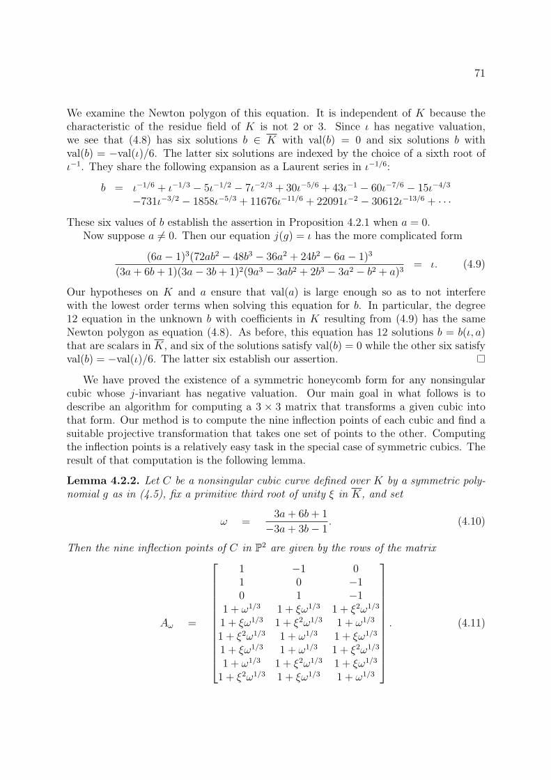
71

We examine the Newton polygon of this equation. It is independent of K because thecharacteristic of the residue field of K is not 2 or 3. Since ι has negative valuation,we see that (4.8) has six solutions b ∈ K with val(b) = 0 and six solutions b withval(b) = −val(ι)/6. The latter six solutions are indexed by the choice of a sixth root ofι−1. They share the following expansion as a Laurent series in ι−1/6:

b = ι−1/6 + ι−1/3 − 5ι−1/2 − 7ι−2/3 + 30ι−5/6 + 43ι−1 − 60ι−7/6 − 15ι−4/3

−731ι−3/2 − 1858ι−5/3 + 11676ι−11/6 + 22091ι−2 − 30612ι−13/6 + · · ·

These six values of b establish the assertion in Proposition 4.2.1 when a = 0.Now suppose a 6= 0. Then our equation j(g) = ι has the more complicated form

(6a− 1)3(72ab2 − 48b3 − 36a2 + 24b2 − 6a− 1)3

(3a+ 6b+ 1)(3a− 3b+ 1)2(9a3 − 3ab2 + 2b3 − 3a2 − b2 + a)3= ι. (4.9)

Our hypotheses on K and a ensure that val(a) is large enough so as to not interferewith the lowest order terms when solving this equation for b. In particular, the degree12 equation in the unknown b with coefficients in K resulting from (4.9) has the sameNewton polygon as equation (4.8). As before, this equation has 12 solutions b = b(ι, a)that are scalars in K, and six of the solutions satisfy val(b) = 0 while the other six satisfyval(b) = −val(ι)/6. The latter six establish our assertion.

We have proved the existence of a symmetric honeycomb form for any nonsingularcubic whose j-invariant has negative valuation. Our main goal in what follows is todescribe an algorithm for computing a 3 × 3 matrix that transforms a given cubic intothat form. Our method is to compute the nine inflection points of each cubic and find asuitable projective transformation that takes one set of points to the other. Computingthe inflection points is a relatively easy task in the special case of symmetric cubics. Theresult of that computation is the following lemma.

Lemma 4.2.2. Let C be a nonsingular cubic curve defined over K by a symmetric poly-nomial g as in (4.5), fix a primitive third root of unity ξ in K, and set

ω =3a+ 6b+ 1

−3a+ 3b− 1. (4.10)

Then the nine inflection points of C in P2 are given by the rows of the matrix

Aω =

1 −1 01 0 −10 1 −1

1 + ω1/3 1 + ξω1/3 1 + ξ2ω1/3

1 + ξω1/3 1 + ξ2ω1/3 1 + ω1/3

1 + ξ2ω1/3 1 + ω1/3 1 + ξω1/3

1 + ξω1/3 1 + ω1/3 1 + ξ2ω1/3

1 + ω1/3 1 + ξ2ω1/3 1 + ξω1/3

1 + ξ2ω1/3 1 + ξω1/3 1 + ω1/3

. (4.11)

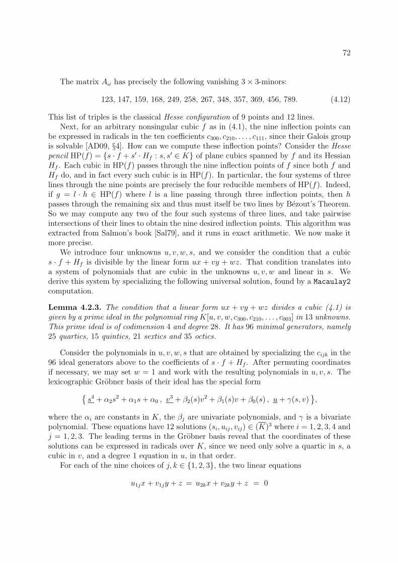
72

The matrix Aω has precisely the following vanishing 3 × 3-minors:

123, 147, 159, 168, 249, 258, 267, 348, 357, 369, 456, 789. (4.12)

This list of triples is the classical Hesse configuration of 9 points and 12 lines.Next, for an arbitrary nonsingular cubic f as in (4.1), the nine inflection points can

be expressed in radicals in the ten coefficients c300, c210, . . . , c111, since their Galois groupis solvable [AD09, §4]. How can we compute these inflection points? Consider the Hessepencil HP(f) = {s · f + s′ ·Hf : s, s′ ∈ K} of plane cubics spanned by f and its HessianHf . Each cubic in HP(f) passes through the nine inflection points of f since both f andHf do, and in fact every such cubic is in HP(f). In particular, the four systems of threelines through the nine points are precisely the four reducible members of HP(f). Indeed,if g = l · h ∈ HP(f) where l is a line passing through three inflection points, then hpasses through the remaining six and thus must itself be two lines by Bezout’s Theorem.So we may compute any two of the four such systems of three lines, and take pairwiseintersections of their lines to obtain the nine desired inflection points. This algorithm wasextracted from Salmon’s book [Sal79], and it runs in exact arithmetic. We now make itmore precise.

We introduce four unknowns u, v, w, s, and we consider the condition that a cubics · f + Hf is divisible by the linear form ux + vy + wz. That condition translates intoa system of polynomials that are cubic in the unknowns u, v, w and linear in s. Wederive this system by specializing the following universal solution, found by a Macaulay2

computation.

Lemma 4.2.3. The condition that a linear form ux + vy + wz divides a cubic (4.1) isgiven by a prime ideal in the polynomial ring K[u, v, w, c300, c210, . . . , c003] in 13 unknowns.This prime ideal is of codimension 4 and degree 28. It has 96 minimal generators, namely25 quartics, 15 quintics, 21 sextics and 35 octics.

Consider the polynomials in u, v, w, s that are obtained by specializing the cijk in the96 ideal generators above to the coefficients of s · f + Hf . After permuting coordinatesif necessary, we may set w = 1 and work with the resulting polynomials in u, v, s. Thelexicographic Grobner basis of their ideal has the special form

{s4 + α2s

2 + α1s+ α0 , v3 + β2(s)v

2 + β1(s)v + β0(s) , u+ γ(s, v)},

where the αi are constants in K, the βj are univariate polynomials, and γ is a bivariatepolynomial. These equations have 12 solutions (si, uij, vij) ∈ (K)3 where i = 1, 2, 3, 4 andj = 1, 2, 3. The leading terms in the Grobner basis reveal that the coordinates of thesesolutions can be expressed in radicals over K, since we need only solve a quartic in s, acubic in v, and a degree 1 equation in u, in that order.

For each of the nine choices of j, k ∈ {1, 2, 3}, the two linear equations

u1jx+ v1jy + z = u2kx+ v2ky + z = 0

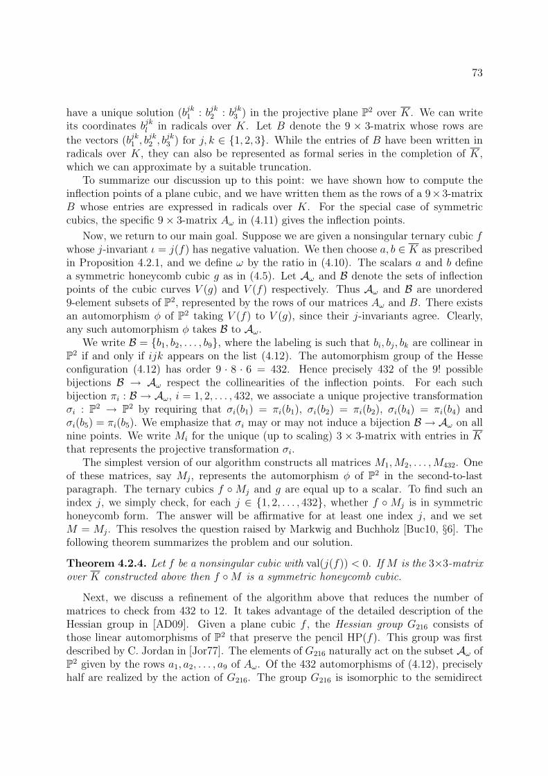
73

have a unique solution (bjk1 : bjk2 : bjk3 ) in the projective plane P2 over K. We can writeits coordinates bjkl in radicals over K. Let B denote the 9 × 3-matrix whose rows are

the vectors (bjk1 , bjk2 , b

jk3 ) for j, k ∈ {1, 2, 3}. While the entries of B have been written in

radicals over K, they can also be represented as formal series in the completion of K,which we can approximate by a suitable truncation.

To summarize our discussion up to this point: we have shown how to compute theinflection points of a plane cubic, and we have written them as the rows of a 9×3-matrixB whose entries are expressed in radicals over K. For the special case of symmetriccubics, the specific 9 × 3-matrix Aω in (4.11) gives the inflection points.

Now, we return to our main goal. Suppose we are given a nonsingular ternary cubic fwhose j-invariant ι = j(f) has negative valuation. We then choose a, b ∈ K as prescribedin Proposition 4.2.1, and we define ω by the ratio in (4.10). The scalars a and b definea symmetric honeycomb cubic g as in (4.5). Let Aω and B denote the sets of inflectionpoints of the cubic curves V (g) and V (f) respectively. Thus Aω and B are unordered9-element subsets of P2, represented by the rows of our matrices Aω and B. There existsan automorphism φ of P2 taking V (f) to V (g), since their j-invariants agree. Clearly,any such automorphism φ takes B to Aω.

We write B = {b1, b2, . . . , b9}, where the labeling is such that bi, bj, bk are collinear inP2 if and only if ijk appears on the list (4.12). The automorphism group of the Hesseconfiguration (4.12) has order 9 · 8 · 6 = 432. Hence precisely 432 of the 9! possiblebijections B → Aω respect the collinearities of the inflection points. For each suchbijection πi : B → Aω, i = 1, 2, . . . , 432, we associate a unique projective transformationσi : P2 → P2 by requiring that σi(b1) = πi(b1), σi(b2) = πi(b2), σi(b4) = πi(b4) andσi(b5) = πi(b5). We emphasize that σi may or may not induce a bijection B → Aω on allnine points. We write Mi for the unique (up to scaling) 3 × 3-matrix with entries in Kthat represents the projective transformation σi.

The simplest version of our algorithm constructs all matrices M1,M2, . . . ,M432. Oneof these matrices, say Mj, represents the automorphism φ of P2 in the second-to-lastparagraph. The ternary cubics f ◦Mj and g are equal up to a scalar. To find such anindex j, we simply check, for each j ∈ {1, 2, . . . , 432}, whether f ◦Mj is in symmetrichoneycomb form. The answer will be affirmative for at least one index j, and we setM = Mj. This resolves the question raised by Markwig and Buchholz [Buc10, §6]. Thefollowing theorem summarizes the problem and our solution.

Theorem 4.2.4. Let f be a nonsingular cubic with val(j(f)) < 0. If M is the 3×3-matrixover K constructed above then f ◦M is a symmetric honeycomb cubic.

Next, we discuss a refinement of the algorithm above that reduces the number ofmatrices to check from 432 to 12. It takes advantage of the detailed description of theHessian group in [AD09]. Given a plane cubic f , the Hessian group G216 consists ofthose linear automorphisms of P2 that preserve the pencil HP(f). This group was firstdescribed by C. Jordan in [Jor77]. The elements of G216 naturally act on the subset Aω ofP2 given by the rows a1, a2, . . . , a9 of Aω. Of the 432 automorphisms of (4.12), preciselyhalf are realized by the action of G216. The group G216 is isomorphic to the semidirect

74

product (Z/3Z)2⋊SL(2, 3). The first factor sends f to itself and permutes Aω transitively.The second factor, of order 24, sends f to each of the 12 cubics in HP(f) isomorphic toit. The quotient of SL(2, 3) by the 2-element stabilizer of f is isomorphic to PSL(2, 3),with 12 elements. Identifying G216 with the subgroup of S9 permuting Aω, a set of cosetrepresentatives for PSL(2, 3) inside G216 consists of the following 12 permutations (incycle notation):

id, (456)(987), (654)(789), (2437)(5698), (246378)(59), (254397)(68)(249)(375), (258)(963), (2539)(4876), (852)(369), (287364)(59), (2836)(4975)

(4.13)

With this notation, an example of an automorphism of the Hesse configuration (4.12)that is not realized by the Hessian group G216 is the permutation τ = (47)(58)(69).

Here is now our refined algorithm for the last step towards Theorem 4.2.4. Letf, g,B,Aω be given as above. For any automorphism ρ of (4.12), we denote by φρ :P2 → P2 the projective transformation (b1, b2, b4, b5) 7→ (aρ(1), aρ(2), aρ(4), aρ(5)). To finda transformation from f to g, we proceed as follows. First, we check to see whether φid

maps B to Aω. (It certainly maps four elements of B to Aω but maybe not all nine). Ifφid(B) = Aω then φid(f) is in the Hesse pencil HP(g). This implies that one of the 12maps φσ, where σ runs over (4.13), takes f to g. If φid(B) 6= Aω then φτ must map B toAω, since G216 has index 2 in the automorphism group of the Hesse configuration and τrepresents the nonidentity coset. Then one of the 12 maps φτσ, where σ runs over (4.13),takes f to g. In either case, after computing φid, we only have to check 12 maps, and oneof them will work.

We close with two remarks. First, the set of matrices M ∈ GL(3, K) that send agiven cubic f into honeycomb form is a rigid analytic variety, since the conditions on theentries of M are inequalities in valuations of polynomial expressions therein. It would beinteresting to study this space further.

The second remark concerns the arithmetic nature of the output of our algorithm. Theentries of the matrix M were constructed to be expressible in radicals over K(ω), withω as in (4.10). However, as it stands, we do not know whether they can be expressed inradicals over the ground field K. The problem lies in the application of Proposition 4.2.1.Our first step was to chose a scalar a ∈ K whose valuation is large enough. Thereafter,we computed b by solving a univariate equation of degree 12. This equation is generallyirreducible with non-solvable Galois group. Perhaps it is possible to choose a and bsimultaneously, in radicals over K, so that (a, b) lies on the curve (4.9), but at present,we do not know how to make this choice.

4.3 Parametrization and implicitization

A standard task of computer algebra is to go back and forth between parametric andimplicit representations of algebraic varieties. Of course, these transformations are mosttransparent when the variety is rational. If the variety is not unirational then para-metric representations typically involve transcendental functions. In this section, we use

75

nonarchimedean theta functions to parametrize planar cubics, we demonstrate how to im-plicitize this parametrization, and we derive an intrinsic characterization of honeycombcubics in terms of their nonarchimedean geometry.

In this section we assume that K is an algebraically closed field which is complete withrespect to a nonarchimedean valuation. Fix a scalar ι ∈ K with val(ι) < 0. Accordingto Tate’s classical theory [Sil94], the unique elliptic curve E over K with j(E) = ι isanalytically isomorphic to K∗/qZ, where q ∈ K∗ is a particular scalar with val(q) > 0,called the Tate parameter of E. The symbol qZ denotes the multiplicative group generatedby q. The Tate parameter of E is determined from the j-invariant by inverting the powerseries relation

j =1

q+ 744 + 196884q + 21493760q2 + · · · (4.14)

This relation can be derived and computed to arbitrary precision from the identity

j =(1 − 48a4(q))

3

∆(q),

where the invariant a4 and the discriminant ∆ are given by

a4(q) = −5∑

n≥1

n3qn

1 − qnand ∆(q) = q

∏

n≥1

(1 − qn)24.

We refer to Silverman’s text book [Sil94] for an introduction to the relevant theory ofelliptic curves, and specifically to [Sil94, Theorems V.1.1, V.3.1] for the above results.

Our aim in this section is to work directly with the analytic representation

E = K∗/qZ,

and to construct its honeycomb embeddings into the plane P2K . In our explicit computa-

tions, scalars in K are presented as truncated power series in a uniformizing parameter.The arithmetic is numerical rather than symbolic. Thus, this section connects the emerg-ing fields of tropical geometry and numerical algebraic geometry.

By a holomorphic function on K∗ we mean a formal Laurent series∑anx

n whichconverges for every x ∈ K∗. A meromorphic function is a ratio of two holomorphicfunctions; they have a well-defined notion of zeroes and poles as usual. A theta functionon K∗, relative to the subgroup qZ, is a meromorphic function on K∗ whose divisor isperiodic with respect to qZ. Hence theta functions on K∗ represent divisors on E. Thefundamental theta function Θ : K∗ → K is defined by

Θ(x) =∏

n>0

(1 − qnx)∏

n≥0

(1 −qn

x).

Note that Θ has a simple zero at the identity of E and no other zeroes or poles. Further-more, given any a ∈ K∗, we define the shifted theta function

Θa(x) = Θ(x/a).

76

The function Θa represents the divisor [a] ∈ DivE, where [a] denotes the point of theelliptic curve E represented by a. One can also check that Θa(x/q) = −x

aΘa(x).

Now suppose D = n1p1 + · · · + nsps is a divisor on E that satisfies deg(D) = 0 andpn1

1 · · · pnss = 1, as an equation in the multiplicative group K∗/qZ. We can use theta

functions to exhibit D as a principal divisor, as follows. Pick lifts p1, . . . , ps ∈ K∗ ofp1, . . . , ps, respectively, such that pn1

1 · · · pnss = 1 as an equation in K∗. Let

f(x) = Θp1(x)n1 · · ·Θps

(x)ns .

This defines a function f : K∗ → K that is q-periodic because

f(x/q) =(−x)n1+···+ns

pn11 · · · pns

s

f(x) = (−x)n1+···+nsf(x) = f(x).

The last equation holds because we assumed that deg(D) = n1 + · · · + ns is zero. Weconclude that f descends to a meromorphic function on K∗/qZ with divisor D.

We now present a parametric representation of plane cubic curves that will work wellfor honeycombs. In what follows, we write (z0 : z1 : z2) for the coordinates on P2. Fixscalars a, b, c, p1, . . . , p9 in K∗ that satisfy the conditions

p1p2p3 = p4p5p6 = p7p8p9 and pi/pj 6∈ qZ for i 6= j. (4.15)

The following defines a map from E = K∗/qZ into the projective plane P2 as follows:

x 7→(a · Θp1Θp2Θp3(x) : b · Θp4Θp5Θp6(x) : c · Θp7Θp8Θp9(x)

). (4.16)

This map embeds the elliptic curve E = K∗/qZ analytically as a plane cubic:

Lemma 4.3.1. If the image of the map (4.16) has three distinct intersection pointswith each of the three coordinate lines {zi = 0}, then it is a cubic curve in P2. Everynonsingular cubic with this property and having Tate parameter q arises this way.

Proof. By construction, the following two functions K∗ → K are q-periodic:

f(x) =a · Θp1Θp2Θp3(x)

c · Θp7Θp8Θp9(x)and g(x) =

b · Θp4Θp5Θp6(x)

c · Θp7Θp8Θp9(x). (4.17)

Hence f and g descend to meromorphic functions on the elliptic curve E = K∗/qZ. Themap (4.16) can be written as x 7→ (f(x) : g(x) : 1) and this defines a map from E into P2.The divisorD = p7+p8+p9 on E has degree 3. By the Riemann-Roch argument in [Har77,Example 3.3.3], its space of sections L(D) is 3-dimensional. Moreover, the assumptionabout having three distinct intersection points implies that the meromorphic functionsf, g and 1 form a basis of the vector space L(D). The image of E in P(L(D)) ≃ P2 is acubic curve because L(3D) is 9-dimensional.

For the second statement, we take C to be any nonsingular cubic curve with Tateparameter q that has distinct intersection points with the three coordinate lines in P2.

77

There exists a morphism φ from the abstract elliptic curve E = K∗/qZ into P2 whoseimage equals C. Let {p1, p2, p3}, {p4, p5, p6} and {p7, p8, p9} be the preimages under φof the triples C ∩ {z0 = 0}, C ∩ {z1 = 0} and C ∩ {z2 = 0} respectively. The divisorsD1 = p1 + p2 + p3 − p7 − p8 − p9 and D2 = p4 + p5 + p6 − p7 − p8 − p9 are principal, andhence p1p2p3

p7p8p9= p4p5p6

p7p8p9= 1 in the multiplicative group E = K∗/qZ. We choose preimages

p1, p2, . . . , p9 in K∗ such that (4.15) holds for these scalars.Our map φ can be written in the form x 7→ (f(x) : g(x) : 1) where div(f) = D1 and

div(g) = D2. By the Abel-Jacobi Theorem (cf. [Roq70, Proposition 1]), the function fis uniquely determined, up to a multiplicative scalar, by the property div(f) = D1, andsimilarly for g and D2. Then there exist γ1, γ2 ∈ K∗ such that

f(x) = γ1Θp1Θp2Θp3(x)

Θp7Θp8Θp9(x)and g(x) = γ2

Θp4Θp5Θp6(x)

Θp7Θp8Θp9(x).

We conclude that φ has the form (4.16).

It is a natural ask to what extent the parameters in the representation (4.16) of aplane cubic are unique. The following result answers this question.

Proposition 4.3.2. Two vectors (a, b, c, p1, . . . , p9) and (a′, b′, c′, p′1, . . . , p′9) in (K∗)12,

both satisfying (4.15), define the same plane cubic if and only if the latter vector can beobtained from the former by combining the following operations:

(a) Permute the sets {p1, p2, p3}, {p4, p5, p6} and {p7, p8, p9}.

(b) Scale each of a, b and c by the same multiplier λ ∈ K∗.

(c) Scale each pi by the same multiplier λ ∈ K∗.

(d) Replace each pi by its multiplicative inverse 1/pi.

(e) Multiply each pi by qni for some ni ∈ Z, where n1+n2+n3 = n4+n5+n6 = n7+n8+n9,

and set a′ = pn11 p

n22 p

n33 a, b

′ = pn44 p

n55 p

n66 b, c

′ = pn77 p

n88 p

n99 c.

Proof. Clearly the relabeling in (a) and the scaling in (b) preserve the curve C ⊂P2. For (c), we note that scaling each pi by the same constant λ ∈ K∗ produces areparametrization of the same curve; only the location of the identity point changes. Forpart (e), note that Θaqi(x) = Θa(q

−ix) = (−x/a)iΘa(x). Suppose (a, b, c, p1, . . . , p9) and(a′, b′, c′, p′1, . . . , p

′9) satisfy the conditions in (e). Then

(a′ · Θp′1Θp′2

Θp′3: b′ · Θp′4

Θp′5Θp′6

: c′ · Θp′7Θp′8

Θp′9)

=

((−x)na′Θp1Θp2Θp3

pn11 p

n22 p

n33

:(−x)nb′Θp4Θp5Θp6

pn44 p

n55 p

n66

:(−x)nc′Θp7Θp8Θp9

pn77 p

n88 p

n99

)

= (a · Θp1Θp2Θp3 : b · Θp4Θp5Θp6 : c · Θp7Θp8Θp9),

where n = n1 + n2 + n3 = n4 + n5 + n6 = n7 + n8 + n9.

78

Finally, for (d), one may check the identity xΘ(x−1) = Θ(x) directly from the defini-tion of the fundamental theta function. In light of (4.15), this implies

(a · Θp1Θp2Θp3 : b · Θp4Θp5Θp6 : c · Θp7Θp8Θp9)

= ( −x3ap1p2p3

Θ(p1x)Θ(p2

x)Θ(p3

x) : −x3b

p4p5p6Θ(p4

x)Θ(p5

x)Θ(p6

x) : −x3c

p7p8p9Θ(p7

x)Θ(p8

x)Θ(p9

x))

= (aΘ 1p1

(1x)Θ 1

p2

( 1x)Θ 1

p3

( 1x) : bΘ 1

p4

( 1x)Θ 1

p5

( 1x)Θ 1

p6

( 1x) : cΘ 1

p7

( 1x)Θ 1

p8

( 1x)Θ 1

p0

( 1x)).

This is the reparametrization of the elliptic curve E under the involution x 7→ 1/x in thegroup law. We have thus proved the if direction of Proposition 4.3.2.

For the only-if direction, we write ψ and ψ′ for the maps E → C ⊂ P2 defined by(a, b, . . . , p9) and (a′, b′, . . . , p′9) respectively. Then (ψ′)−1 ◦ ψ is an automorphism of theelliptic curve E. The j-invariant of E is neither of the special values 0 or 1728. By[Sil86, Theorem 10.1], the only automorphisms of E are the involution x 7→ 1/x andmultiplication by some fixed element in the group law. These are precisely the operationswe discussed above, and they can be realized by the transformations from (a, b, . . . , p9)to (a′, b′, . . . , p′9) that are described in (c) and (d).

Finally, if (ψ′)−1 ◦ψ is the identity on E, then plugging in x = pi for i = 1, 2, 3 showsthat pi is a zero of aΘp1Θp2Θp3 and hence of a′Θp′1

Θp′2Θp′3

. The same holds for i = 4, 5, 6and i = 7, 8, 9. This accounts for the operations (a), (b) and (e).

Our main result in this section is the following characterization of honeycomb curves,in terms of the analytic representation of plane cubics in (4.16). Writing S1 for the circle,

let V : K∗ → S1 denote the composition K∗ val→ R → R/val(q) ≃ S1.

Theorem 4.3.3. Let a, b, c, p1, . . . , p9 ∈ K∗ as in Lemma 4.3.1. Suppose the valuesV(p1), . . . ,V(p9) occur in cyclic order on S1, with V(p3) = V(p4),V(p6) = V(p7), V(p9) =V(p1), and all other values V(pi) are distinct. Then the image of the map (4.16) isan elliptic curve in honeycomb form. Conversely, any elliptic curve in honeycomb formarises in this manner, after a suitable permutation of the indices.

We shall present two alternative proofs of Theorem 4.3.3. These will highlight differ-ent features of honeycomb curves and how they relate to the literature. The first proof iscomputational and relates our study to the tropical theta functions studied by Mikhalkinand Zharkov [MZ07]. The second proof is more conceptual. It is based on the nonar-chimedean Poincare-Lelong formula for Berkovich curves [BPR11, Theorem 5.68]. Bothapproaches were suggested to us by Matt Baker.

First proof of Theorem 4.3.3. We shall examine the naive tropicalization of the ellipticcurve E = K∗/qZ under its embedding (4.16) into P2. Set Q = val(q) ∈ R>0. If a ∈ K∗

with A = val(a) ∈ R then the tropicalization of the theta function Θa : K∗ → K isobtained by replacing the infinite product of binomials in the definition of Θ(x) by aninfinite sum of pairwise minima. The result is the function

trop(Θa) : R → R , X 7→∑

n>0

min(0, nQ+X−A) +∑

n≥0

min(0, nQ+A−X). (4.18)

79

For any particular real number X, only finitely many summands are non-zero, and hencetrop(Θa)(X) is a well-defined real number. A direct calculation shows that

trop(Θa)(X) = min

{m2 −m

2·Q+m · (A−X) : m ∈ Z

}. (4.19)

Indeed, the distributive law transforms the tropical product of binomials on the right handside of (4.18) into the tropical sum in (4.19). The representation (4.19) is essentially thesame as the tropical theta function of Mikhalkin and Zharkov [MZ07].

The tropical theta function is a piecewise linear function on R, and we can translate(4.19) into an explicit description of the linear pieces of its graph. We find

trop(Θa)(X) =m2 −m

2·Q+m · (A−X) (4.20)

where m is the unique integer satisfying mQ ≤ A − X < (m + 1)Q. In particular, forarguments X in this interval, the function is linear with slope −m.

The tropical theta function approximates the valuation of the theta function. Thesetwo functions agree unless there is some cancellation because the two terms in somebinomial factor of Θa have the same order.

The gap between the tropical theta function and the valuation of the theta functionis crucial in understanding the tropical geometry of the map V : K∗ → S1. Our nextdefinition makes this precise. If x, y ∈ K∗ with V(x) = V(y) then we set

δ(x, y) := val(1 −

x

yqi)

(4.21)

where i ∈ Z is the unique integer satisfying val(x) + val(qi) = val(y). It is easy tocheck that the quantity defined in (4.21) is symmetric, i.e. δ(x, y) = δ(y, x). With thisnotation, the following formula characterizes the gap between the tropical theta functionand the valuation of the theta function. For any a, x ∈ K∗, we have

val(Θa(x)

)− trop(Θa)(val(x)) =

{δ(x, a) if V(a) = V(x),

0 otherwise.(4.22)

Consider now any three scalars x, y, z ∈ K∗ that lie in the same fiber of the map fromK∗ onto the unit circle S1. In symbols, V(x) = V(y) = V(z). Then

the minimum of δ(x, y), δ(x, y) and δ(y, z) is attained twice. (4.23)

This follows from the identity

(xqi − yqj) + (yqj − z) + (z − xqi) = 0

where i, j ∈ Z are defined by val(x) + val(qi) = val(y) + val(qj) = val(z).We are now prepared to prove Theorem 4.3.3. Set Q = val(q). For i = 1, 2, . . . , 9, let

Pi = val(pi) and write Pi = niQ+ ri where ni ∈ Z and ri ∈ [0, Q). Rescaling the pi’s by

80

a common factor and inverting them all does not change the cubic curve, by Proposition4.3.2. After performing such operations if needed, we can assume

0 = r9 = r1 < r2 < r3 = r4 < r5 < r6 = r7 < r8 < Q. (4.24)

The hypothesis (4.15) implies

r1 + r2 + r3 ≡ r4 + r5 + r6 ≡ r7 + r8 + r9 (mod Q).

Together with the chain of inequalities in (4.24), this implies

r1 + r2 + r3 = r4 + r5 + r6 −Q = r7 + r8 + r9 −Q,n1 + n2 + n3 = n4 + n5 + n6 + 1 = n7 + n8 + n9 + 1.

(4.25)

We now examine the naive tropicalization R → TP2 of our map (4.16). It equals

X 7→

(A+ trop(Θp1)(X) + trop(Θp2)(X) + trop(Θp3)(X) :B + trop(Θp4)(X) + trop(Θp5)(X) + trop(Θp6)(X) :C + trop(Θp7)(X) + trop(Θp8)(X) + trop(Θp9)(X)

).

(4.26)

Here A = val(a), B = val(b), C = val(c). The image of this piecewise-linear map coincideswith the tropicalization of the image of (4.16) for generic values of X = val(x). Indeed, ifX lies in the open interval (0, r2) then, by (4.20), the map (4.26) is linear and its imagein the tropical projective plane TP2 is a segment with slope

(−n1 − n2 − n3 − 1 : −n4 − n5 − n6 : n7 − n8 − n9 − 1) = ( 1 : 1 : 0 ).

Here we fix tropical affine coordinates with last coordinate 0. Similarly,

• the slope is (0 : 1 : 0) for X ∈ (r2, r3),

• the slope is (−1 : 0 : 0) for X ∈ (r4, r5),

• the slope is (−1 : −1 : 0) for X ∈ (r5, r6),

• the slope is (0 : −1 : 0) for X ∈ (r7, r8),

• the slope is (1 : 0 : 0) for X ∈ (r8, Q).

These six line segments form a hexagon in TP2. The vertices of that hexagon are theimages of the six distinct real numbers ri in (4.24) under the map (4.26).

Finally, we examine the special values x ∈ K∗ for which the naive tropicalization(4.26) does not compute the correct image in TP2. This happens precisely when some ofthe nine theta functions in (4.16) have a valuation gap when passing to (4.26).

Suppose, for instance, that V(x) = V(p1) = V(p9). From (4.22) we have

val(Θpi

(x))− trop(Θpi

)(val(x)) =

{δ(x, pi) if i = 1 or i = 9,

0 if i 6= 1, 9.(4.27)

81

1

2

34

5

6 7

8

9

Figure 4.2: The Berkovich skeleton Σ of an elliptic curve with honeycomb punctures

We know from (4.23) that the minimum of δ(p1, p9), δ(x, p1), δ(x, p9) is achieved twice.Moreover, by varying the choice of the scalar x with V(x) = r1, the latter two quantitiescan attain any non-negative value that is compatible with this constraint. This shows thatthe image of the set of such x under the tropicalization of the map (4.16) consists of onebounded segment and two rays in TP2. The segment meets the hexagon described aboveat the vertex corresponding to r1 = r9, and consists of the images of the points x such thatδ(p1, p9) ≥ δ(p1, x) = δ(p9, x). Since Θp1 and Θp9 occur in the first and third coordinates,respectively, of (4.16), the slope of the segment is (1 : 0 : 1), and its length is δ(p1, p9).Similarly, the image of the points x such that δ(p1, x) ≥ δ(p1, p9) = δ(p9, x) is a ray ofslope (1 : 0 : 0), and the image of the points x such that δ(p9, x) ≥ δ(p1, p9) = δ(p1, x) isa ray of slope (0 : 0 : 1). Note that these three slopes obey the balancing condition fortropical curves.

A similar analysis determines all six connected components of the complement of thehexagon in the tropical curve, and we see that the tropical curve is a honeycomb whenthe asserted conditions on a, b, c, p1, p2, . . . , p9 are satisfied.

The derivation of the converse direction, that any honeycomb cubic has the desiredparametrization, will be deferred to the second proof. It seems challenging to prove thiswithout [BPR11]. See also the problem stated at the end of this section.

Second proof of Theorem 4.3.3. We work in the setting of Berkovich curves introducedby Baker, Payne and Rabinoff in [BPR11]. Let Ean denote the analytification of theelliptic curve E, and let Σ denote the minimal skeleton of Ean, as defined in [BPR11,§5.14], with respect to the given set D = {p1, p2, . . . , p9} of nine punctures. Our standingassumption val(j) < 0 ensures that the Berkovich curve Ean contains a unique cycle S1,and Σ is obtained from that cycle by attaching trees with nine leaves in total. In close

82

analogy to [BPR11, §7.1], we consider the retraction map onto S1:

E(K)\D → Ean\D → Σ → R/val(q)Z ≃ S1.

The condition in Theorem 4.3.3 states that, under this map, the points of E(K) given byp1, p2, . . . , p9 retract to six distinct points on S1, in cyclic order with fibers

{p9, p1}, {p2}, {p3, p4}, {p5}, {p6, p7}, {p8}.

This means that Σ looks precisely like the graph in Figure 4.2. This picture is theBerkovich model of a honeycomb cubic. To see this, we shall apply the nonarchimedeanPoincare-Lelong Formula [BPR11, Theorem 5.69] in conjunction with a combinatorialargument about balanced graphs in R2.

The rational functions f and g in (4.17) are well-defined on Ean\D, and we mayconsider the negated logarithms of their norms: F = −log|f | and G = −log|g|. Ourtropical curve can be identified with its image in R2 under the map (F,G). Accordingto part (1) of [BPR11, Theorem 5.69], this map factors through the retraction of Ean\Donto Σ. By part (2), the function (F,G) is linear on each edge of Σ.

We shall argue that the graph Σ in Figure 4.2 is mapped isometrically onto a tropicalhoneycomb curve in R2. Using part (5) of [BPR11, Theorem 5.69], we can determine theslopes of the nine unbounded edges. Namely, F has slope 1 on the rays in Σ towardsp1, p2 and p3, and slope −1 on the rays towards p7, p8 and p9. Similarly, G has slope 1 onthe rays in Σ towards p4, p5 and p6, and slope −1 on the rays towards p7, p8 and p9. Bypart (4), the functions F and G are harmonic, which means that the image in R2 satisfiesthe balancing condition of tropical geometry. This requirement uniquely determines theslopes of the nine bounded edges in the image of Σ. For the three edges not on thecycle this is immediate, and for the six edges on the cycle, this follows by solving a linearsystem of equations. The unique solution to these constraints is a balanced planar graphthat must be a honeycomb cubic. Conversely, every tropical honeycomb cubic in R2 istrivalent with all multiplicities one. By [BPR11, Corollary 6.27(1)], the skeleton Σ mustlook like Figure 4.2, and the corresponding map (F,G) is an isometry onto the cubic.

In the rest of Section 3, we discuss computational aspects of the representation ofplane cubics given in Lemma 4.3.1 and Theorem 4.3.3. We begin with the implicitizationproblem: Given a, b, c, p1, . . . , p9 ∈ K∗, how can we compute the implicit equation (4.1)?Write

(f(x) : g(x) : h(x)

)for the analytic parametrization in (4.16). Then we seek to

compute the unique (up to scaling) coefficients cijk in a K-linear relation

c300f(x)3 + c210f(x)2g(x) + c120f(x)g(x)2

+ c030g(x)3 + c021g(x)

2h(x) + c012g(x)h(x)2 + c003h(x)

3

+ c102f(x)h(x)2 + c201f(x)2h(x) + c111f(x)g(x)h(x) = 0.(4.28)

Evaluating this relation at x = pi, and noting that Θpi(pi) = 0, we get nine linear

equations for the nine cijk’s other than c111. These equations are

c300f(pi)3 + c210f(pi)

2g(pi) + c120f(pi)g(pi)2 + c030g(pi)

3 = 0 for i = 7, 8, 9,c003h(pi)

3 + c102f(pi)h(pi)2 + c201f(pi)

2h(pi) + c300f(pi)3 = 0 for i = 4, 5, 6,

c030g(pi)3 + c021g(pi)

2h(pi) + c012g(pi)h(pi)2 + c003h(pi)

3 = 0 for i = 1, 2, 3.

83

The first group of equations has a solution (c300, c210, c120, c030) that is unique up to scaling.Namely, the ratios c300/c030, c210/c030, c120/c030 are the elementary symmetry functions inthe three quantities

b · Θ(p7p4

)Θ(p7p5

)Θ(p7p6

)

a · Θ(p7p1

)Θ(p7p2

)Θ(p7p3

),b · Θ(p8

p4)Θ(p8

p5)Θ(p8

p6)

a · Θ(p8p1

)Θ(p8p2

)Θ(p8p3

)and

b · Θ(p9p4

)Θ(p9p5

)Θ(p9p6

)

a · Θ(p9p1

)Θ(p9p2

)Θ(p9p3

).

The analogous statements hold for the second and third group of equations.We are thus left with computing the middle coefficient c111 in the relation (4.28). We

do this by picking any v ∈ K with f(v)g(v)h(v) 6= 0. Then (4.28) gives

c111 = −1

f(v)g(v)h(v)

(c300f(v)3 + c210f(v)2g(v) + · · · + c201f(v)2h(v)

).

We have implemented this implicitization method in Mathematica, for input data inthe field K = Q(t) of rational functions with rational coefficients.

The parameterization problem is harder. Here we are given the 10 coefficients cijk ofa honeycomb cubic that has three distinct intersection points with each coordinate linez0 = 0, z1 = 0, z2 = 0. The task is to compute 12 scalars a, b, c, p1, . . . , p9 ∈ K∗ thatrepresent the cubic as in Lemma 4.3.1. The 12 output scalars are not unique, but thedegree of non-uniqueness is characterized exactly by Proposition 4.3.2. This task amountsto solving an analytic system of equations. We shall leave it to a future project to designan algorithm for doing this in practice.

4.4 The tropical group law

In this section, we present a combinatorial description of the group law on a honeycombelliptic curve based on the parametric representation in Section 3. We start by studyingthe inflection points of such a curve. We continue to assume that K is algebraically closedand complete with respect to a nonarchimedean valuation.

Let Eψ

−→ C ⊂ P2 be a honeycomb embedding of the abstract elliptic curve E =K∗/qZ. Let v1, v2, v3, v4, v5 and v6 denote the vertices of the hexagon in the tropical cubictrop(C), labeled as in Figure 4.3. Let ei denote the edge between vi and vi+1, with theconvention v7 = v1, and let ℓi denote the lattice length of ei. By examining the widthand height of the hexagon, we see that the six lattice lengths ℓ1, ℓ2, ℓ3, ℓ4, ℓ5, ℓ6 satisfy twolinearly independent relations:

ℓ1 + ℓ2 = ℓ4 + ℓ5 and ℓ2 + ℓ3 = ℓ5 + ℓ6.

We first prove the following basic fact about the inflection points on the cubic C.

Lemma 4.4.1. The tropicalizations of the nine inflection points of the cubic curve C ⊂ P2

retract to the hexagonal cycle of trop(C) ⊂ R2 in three groups of three.

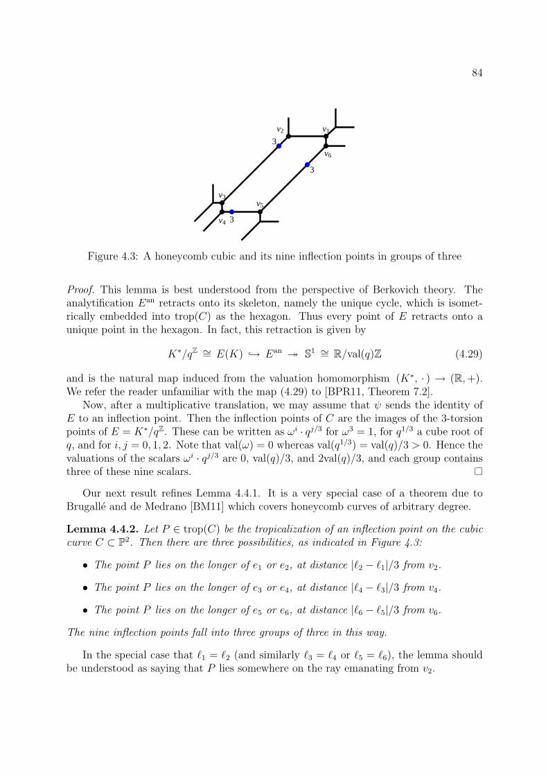
84

v1v2

v3

v4

v5

v6

3

3

3

Figure 4.3: A honeycomb cubic and its nine inflection points in groups of three

Proof. This lemma is best understood from the perspective of Berkovich theory. Theanalytification Ean retracts onto its skeleton, namely the unique cycle, which is isomet-rically embedded into trop(C) as the hexagon. Thus every point of E retracts onto aunique point in the hexagon. In fact, this retraction is given by

K∗/qZ ∼= E(K) → Ean։ S1 ∼= R/val(q)Z (4.29)

and is the natural map induced from the valuation homomorphism (K∗, · ) → (R,+).We refer the reader unfamiliar with the map (4.29) to [BPR11, Theorem 7.2].

Now, after a multiplicative translation, we may assume that ψ sends the identity ofE to an inflection point. Then the inflection points of C are the images of the 3-torsionpoints of E = K∗/qZ. These can be written as ωi · qj/3 for ω3 = 1, for q1/3 a cube root ofq, and for i, j = 0, 1, 2. Note that val(ω) = 0 whereas val(q1/3) = val(q)/3 > 0. Hence thevaluations of the scalars ωi · qj/3 are 0, val(q)/3, and 2val(q)/3, and each group containsthree of these nine scalars.

Our next result refines Lemma 4.4.1. It is a very special case of a theorem due toBrugalle and de Medrano [BM11] which covers honeycomb curves of arbitrary degree.

Lemma 4.4.2. Let P ∈ trop(C) be the tropicalization of an inflection point on the cubiccurve C ⊂ P2. Then there are three possibilities, as indicated in Figure 4.3:

• The point P lies on the longer of e1 or e2, at distance |ℓ2 − ℓ1|/3 from v2.



The nine inflection points fall into three groups of three in this way.

In the special case that ℓ1 = ℓ2 (and similarly ℓ3 = ℓ4 or ℓ5 = ℓ6), the lemma shouldbe understood as saying that P lies somewhere on the ray emanating from v2.

85

Proof. Consider the tropical line whose node lies at v2, and let L be any classical linein P2

K that is generic among lifts of that tropical line. Then the three points in L ∩ Ctropicalize to the stable intersection points of trop(L) with trop(C), namely the verticesv1, v2 and v3. Let x denote the counterclockwise distance along the hexagon from v2 toP . By applying a multiplicative translation in E, we fix the identity to be an inflectionpoint on C that tropicalizes to P . Then v1 + v2 + v3 = 0 in the group S1 ≃ R/val(q)Z.This observation implies the congruence relation

(ℓ1 + x) + x+ (x− ℓ2) ≡ 0 mod val(q),

and hence 3x ≡ ℓ2 − ℓ1. One solution to this congruence is x = (ℓ2 − ℓ1)/3. This meansthat the point P lies on the longer edge, e1 or e2, at distance |ℓ1 − ℓ2|/3 from v2. Theanalysis is identical for the vertex v4 and for the vertex v6, and it identifies two otherlocations on S1 for retractions of inflection points.

Next, we wish to review some basic facts about the group structures on a plane cubiccurve C. The abstract elliptic curve E = K∗/qZ is an abelian group, in the obvioussense, as a quotient of the abelian group (K∗, · ). Knowledge of that group structure isequivalent to knowing the surface {(r, s, t) ∈ E3 : r · s · t = qZ}.

The group structure on E induces a group structure (C, ⋆ ) on the plane cubic curveC = ψ(E). While the isomorphism ψ is analytic, the group operation on C is actuallyalgebraic. Equivalently, the set {(u, v, w) ∈ C3 : u ⋆ v ⋆ w = id} is an algebraic surfacein (P2)3. However, this surface depends heavily on the choice of parametrization ψ.Different isomorphisms from the abstract elliptic curve E onto the plane cubic C willresult in different group structures in P2.

The most convenient choices of ψ are those that send the identity element qZ of E toone of the nine inflection points of C. Such maps ψ are characterized by the conditionthat u ⋆ v ⋆ w = id if and only if u, v and w are collinear in P2. If so, the data of thegroup law can be recorded in the surface

{(u, v, w) ∈ C3 : u, v and w lie on a line in P2

}⊂ (P2)3. (4.30)

We emphasize, however, that we have no reason to assume a priori that the identityelement id = ψ(qZ) on the plane cubic C is an inflection point: every point on C isthe identity in some group law. Indeed, we can simply replace ψ by its compositionwith a translation x 7→ r · x of the group E. Our analysis below covers all cases:our combinatorial description of the group law on trop(C) is always valid, regardless ofwhether the identity is an inflection point or not.

A partial description of the tropical group law was given by Vigeland in [Vig09].Specifically, his choice of the fixed point O corresponds to the point trop(ψ(qZ)). Vige-land’s group law is a combinatorial extension of the polyhedral surface

{(U, V,W ) ∈ S1 × S1 × S1 : U + V +W = O

}(4.31)

This torus comes with a distinguished subdivision into polygons since S1 has been iden-tified with the hexagon. The polyhedral torus (4.31) is illustrated in Figure 4.4.

86

Figure 4.4: The torus in the tropical group law surface (4.31). The two pictures representthe honeycomb cubic and the symmetric honeycomb cubic shown in Figure 4.1.

Our goal is to characterize the tropical group law as follows. For a given honeycombembedding ψ : E → P2, we define the tropical group law surface to be

TGL(ψ) ={(trop(ψ(x)), trop(ψ(y)), trop(ψ(z))) : x, y, z ∈ E, x · y · z = id

}⊂ (R2)3.

If ψ sends the identity to an inflection point, then this is the tropicalization of (4.30):

TGL(ψ) = {(trop(u), trop(v), trop(w)) : u, v, w ∈ C lie on a line in P2} ⊂ (R2)3.

The tropical group law surface is a tropical algebraic variety of dimension 2, and canin principle be computed, for K = Q(t), using the software gfan [Jen]. This surfacecontains all the information of the tropical group law. We shall explain how TGL(ψ) canbe computed combinatorially, even if ψ(id) is not an inflection point.

Our approach follows directly from Section 3. Let ψ : E → P2 be a honeycomb

embedding of an elliptic curve E, and let V : K∗ → S1 denote the composition K∗ val→ R →

R/val(q) ≃ S1. By Theorem 4.3.3, there exist a, b, c, p1, . . . , p9 ∈ K∗ with V(p1), . . . ,V(p9)occurring in cyclic order on S1, with V(p3) = V(p4),V(p6) = V(p7),V(p9) = V(p1), andall other values V(pi) distinct, such that ψ is given by

x 7→(a · Θp1Θp2Θp3(x) : b · Θp4Θp5Θp6(x) : c · Θp7Θp8Θp9(x)

).

Now, again as in Section 3, given x, y ∈ K∗ with V(x) = V(y), we set

δ(x, y) = val(1 −

x

yqi),

where i ∈ Z is specified by val(x)+val(qi) = val(y). We have seen that if x ∈ K∗ satisfiesV(x) = V(pi), then trop(x) lies at distance δ(x, pi) from the hexagon along the tentacle

87

associated to pi. By the tentacle of pi we mean the union of the ray associated to pi andthe bounded segment to which that ray is attached.

The next proposition is our main result in Section 4. We shall construct the tropicalgroup law surface by way of its projection to the first two coordinates

π : TGL(ψ) → trop(C) × trop(C) ⊂ (R2)2.

As before, we identify the hexagon of trop(C) with the circle S1 ≃ R/val(q). GivenU, V ∈ trop(C), let U ◦ V ∈ S1 denote the sum of the retractions of U and V to thehexagon. The location of U ◦V depends on the choice of ψ and in particular the locationof O = trop(ψ(id)) on the hexagon S1. Let −(U ◦ V ) denote the inverse of U ◦ V , againunder addition on S1. By the distance of a point U ∈ trop(C) to the hexagon S1 we meanthe lattice length of the unique path in trop(C) from U to S1. Finally, we say that u ∈ K∗

is a lift of U ∈ trop(C) if trop(ψ(u · qZ)) = U . The following proposition characterizesthe fiber of the map π over a given pair (U, V ).

Proposition 4.4.3. Let ψ : E → C ⊂ P2 be a honeycomb embedding, with the operation◦ : trop(C) × trop(C) → S1 defined as above, and “is a vertex” refers to the hexagon S1.For any U and V ∈ trop(C), exactly one of the following occurs:

(i) If −(U ◦ V ) is not a vertex, then π−1(U, V ) is the singleton {−(U ◦ V )}.

(ii) If −(U ◦ V ) is a vertex adjacent to a single unbounded ray Ri towards the point pi,then π−1(U, V ) is the set of points on Ri whose distance to S1 equals δ(u−1v−1, pi)for some lifts u, v ∈ K∗ of U and V .

(iii) If −(U ◦ V ) is a vertex adjacent to a bounded segment B, along with two rays Rj

and Rk, toward the points pj and pk, then π−1(U, V ) consists of

• the points on B whose distance to S1 is equal to δ(u−1v−1, pj) = δ(u−1v−1, pk)for some lifts u, v ∈ K∗ of U and V ,

• the points on Rj whose distance to S1 is equal to δ(u−1v−1, pj) > δ(u−1v−1, pk)for some lifts u, v ∈ K∗ of U and V , and

• the points on Rk whose distance to S1 is equal to δ(u−1v−1, pk) > δ(u−1v−1, pj)for some lifts u, v ∈ K∗ of U and V .

Proof. For any lifts u, v ∈ K∗ of U, V , we have V(u−1v−1) + V(u) + V(v) = 0 in S1 =R/val(q)Z. This equation determines the retraction −(U◦V ) of the point trop(ψ(u−1v−1))to the hexagon. If −(U ◦ V ) is not a vertex, then trop(ψ(u−1v−1)) must be precisely thepoint −(U ◦ V ), as no other points retract to it.

If instead −(U ◦V ) is a vertex of the hexagon, then we either have V(u−1v−1) = V(pi)for exactly one pi, or V(u−1v−1) = V(pj) = V(pk) for exactly two points pj and pk,depending on whether one or two rays emanate from −(U ◦V ). We have seen (in our firstproof of Theorem 4.3.3) that the distance of trop(ψ(u−1v−1)) to the hexagon, measuredalong the tentacle associated to pi, is δ(u−1v−1, pi). In either case, these distances uniquelydetermine the location of trop(ψ(u−1v−1)).

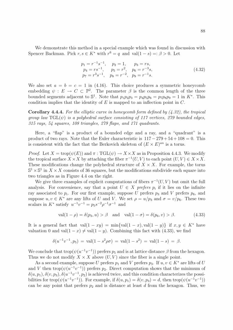
88

We demonstrate this method in a special example which was found in discussion withSpencer Backman. Pick r, s ∈ K∗ with r6 = q and val(1 − s) =: β > 0. Let

p1 = r−1s−1, p2 = 1, p3 = rs,p4 = rs−1, p5 = r2, p6 = r−3s,p7 = r3s−1, p8 = r−2, p9 = r−1s.

(4.32)

We also set a = b = c = 1 in (4.16). This choice produces a symmetric honeycombembedding ψ : E → C ⊂ P2. The parameter β is the common length of the threebounded segments adjacent to S1. Note that p1p2p3 = p4p5p6 = p7p8p9 = 1 in K∗. Thiscondition implies that the identity of E is mapped to an inflection point in C.

Corollary 4.4.4. For the elliptic curve in honeycomb form defined by (4.32), the tropicalgroup law TGL(ψ) is a polyhedral surface consisting of 117 vertices, 279 bounded edges,315 rays, 54 squares, 108 triangles, 279 flaps, and 171 quadrants.

Here, a “flap” is a product of a bounded edge and a ray, and a “quadrant” is aproduct of two rays. Note that the Euler characteristic is 117− 279+54+108 = 0. Thisis consistent with the fact that the Berkovich skeleton of (E × E)an is a torus.

Proof. Let X = trop(ψ(E)) and π : TGL(ψ) → X×X as in Proposition 4.4.3. We modifythe tropical surface X×X by attaching the fiber π−1(U, V ) to each point (U, V ) ∈ X×X.These modifications change the polyhedral structure of X ×X. For example, the torusS1 ×S1 in X×X consists of 36 squares, but the modifications subdivide each square intotwo triangles as in Figure 4.4 on the right.

We give three examples of explicit computations of fibers π−1(U, V ) but omit the fullanalysis. For convenience, say that a point U ∈ X prefers pi if it lies on the infiniteray associated to pi. For our first example, suppose U prefers p3 and V prefers p6, andsuppose u, v ∈ K∗ are any lifts of U and V . We set ρ = u/p3 and σ = v/p6. These twoscalars in K∗ satisfy u−1v−1 = p5s

−2ρ−1σ−1 and

val(1 − ρ) = δ(p3, u) > β and val(1 − σ) = δ(p6, v) > β. (4.33)

It is a general fact that val(1 − xy) = min{val(1 − x), val(1 − y)} if x, y ∈ K∗ havevaluation 0 and val(1 − x) 6= val(1 − y). Combining this fact with (4.33), we find

δ(u−1v−1, p5) = val(1 − s2ρσ) = val(1 − s2) = val(1 − s) = β.

We conclude that trop(ψ(u−1v−1)) prefers p5 and is at lattice distance β from the hexagon.Thus we do not modify X ×X above (U, V ) since the fiber is a single point.

As a second example, suppose U prefers p1 and V prefers p3. If u, v ∈ K∗ are lifts of Uand V then trop(ψ(u−1v−1)) prefers p2. Direct computation shows that the minimum ofδ(u, p1), δ(v, p3), δ(u

−1v−1, p2) is achieved twice, and this condition characterizes the possi-bilities for trop(ψ(u−1v−1)). For example, if δ(u, p1) = δ(v, p3) = d, then trop(ψ(u−1v−1))can be any point that prefers p2 and is distance at least d from the hexagon. Thus, we

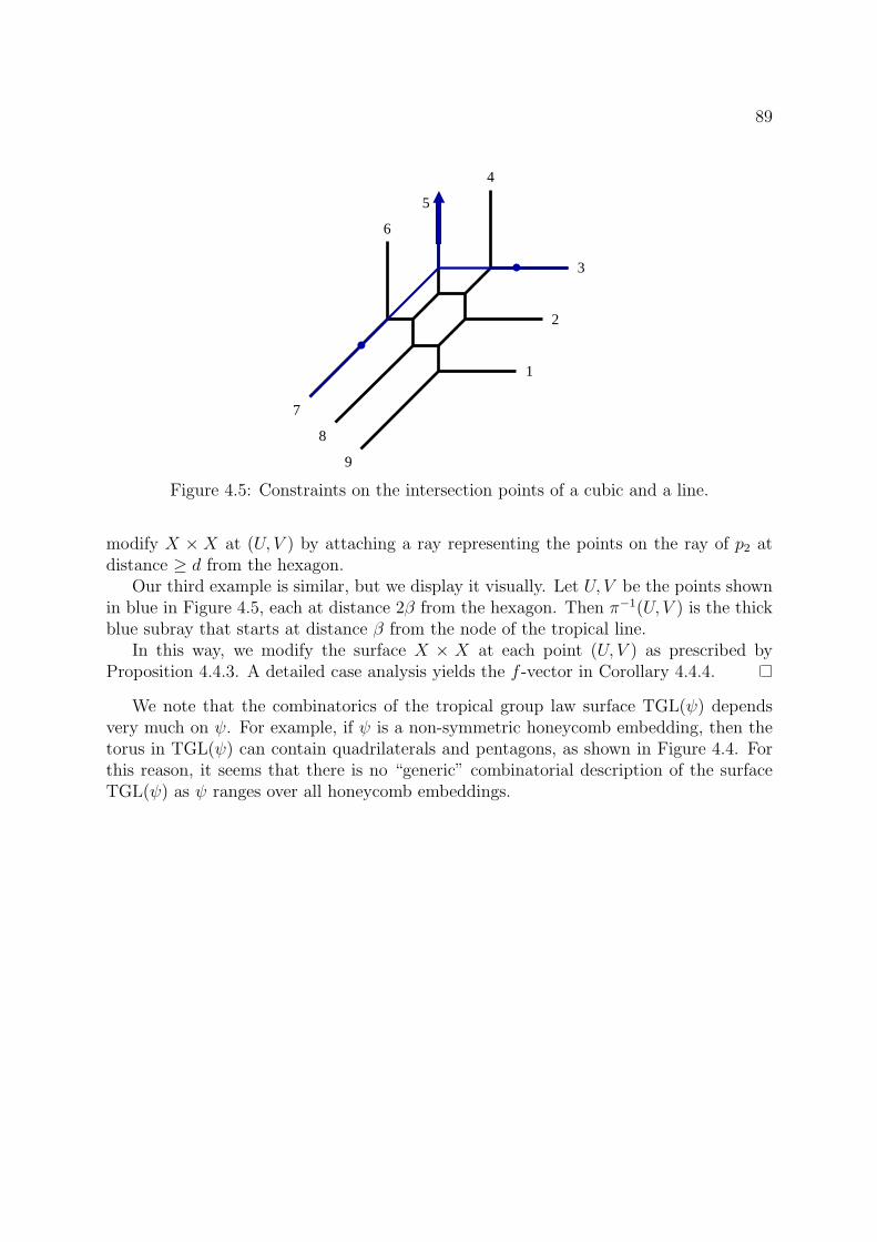
89

9

1

2

3

4

5

6

7

8

Figure 4.5: Constraints on the intersection points of a cubic and a line.

modify X × X at (U, V ) by attaching a ray representing the points on the ray of p2 atdistance ≥ d from the hexagon.

Our third example is similar, but we display it visually. Let U, V be the points shownin blue in Figure 4.5, each at distance 2β from the hexagon. Then π−1(U, V ) is the thickblue subray that starts at distance β from the node of the tropical line.

In this way, we modify the surface X × X at each point (U, V ) as prescribed byProposition 4.4.3. A detailed case analysis yields the f -vector in Corollary 4.4.4.

We note that the combinatorics of the tropical group law surface TGL(ψ) dependsvery much on ψ. For example, if ψ is a non-symmetric honeycomb embedding, then thetorus in TGL(ψ) can contain quadrilaterals and pentagons, as shown in Figure 4.4. Forthis reason, it seems that there is no “generic” combinatorial description of the surfaceTGL(ψ) as ψ ranges over all honeycomb embeddings.

90

Chapter 5

Tropical bases and determinantal

varieties

This chapter is based on the paper “The 4× 4 minors of a 5×n matrix are a tropicalbasis” [CJR09] with Anders N. Jensen and Elena Rubei.

5.1 Introduction

The tropical semi-ring (R,⊕,⊙), consisting of the real numbers equipped with tropicaladdition and multiplication

x⊕ y := min(x, y) and x⊙ y := x+ y for all x, y ∈ R,

gives rise to three distinct notions of rank of a tropical matrix A ∈ Rd×n. These, tropicalrank, Kapranov rank, and Barvinok rank, were studied in [DSS05]. They arise as thetropicalizations of three equivalent characterizations of matrix rank in the usual sense.

Indeed, classically, a d×nmatrix with entries in a fieldK has rank at most r if and onlyif all of its (r+1)×(r+1) submatrices are singular. Equivalently, the set of d×n matricesof rank at most r is the determinantal variety defined by the ideal Jdnr ⊆ K[x11, . . . , xdn]generated by the (r + 1) × (r + 1) minors of a d × n-matrix of variables. Finally, thisalgebraic variety is the image of the matrix product map φ : Kd×r ×Kr×n → Kd×n.

Accordingly, the set of matrices of tropical rank ≤ r is defined to be the intersection ofthe tropical hypersurfaces defined by the (r+ 1)× (r+ 1) minors in K[x11, . . . , xdn]. Theset of matrices of Kapranov rank ≤ r is defined to be the tropical variety T (Jdnr ), whilethe set of matrices of Barvinok rank ≤ r is the image of the tropicalization of φ. We willrevisit these definitions in Section 5.2. We note that T (Jdnr ) can be regarded as the spaceof n labeled points in TPd−1 (defined in Section 2) for which there exists a tropicalizedr− 1 plane containing them; here, we consider matrices up to the equivalence relation oftropically scaling columns.

Since the intersection of the tropical hypersurfaces defined by a set of polynomialsdoes not always equal the tropical variety of the ideal they generate, we do not expect

91

Kapranov rank and tropical rank to be the same. Similarly, the tropicalization of theimage of a polynomial function is not always equal to the image of its tropicalization;therefore, we do not expect Barvinok rank and Kapranov rank to be the same. However,in both of these cases one containment is true, implying

Tropical rank(A) ≤ Kapranov rank(A) ≤ Barvinok rank(A). (5.1)

as shown in [DSS05, Theorem 1.4].We are interested in studying Kapranov rank and tropical rank. The question of

whether these coincide is really a question about tropical bases. Recall that a tropicalbasis for an ideal I ⊆ K[x1, . . . , xn], where K is the field of generalized Laurent seriesto be defined in Section 2, is a finite generating set with hypersurface intersection equalto T (I). The authors of [BJSST07] prove that any ideal I generated by polynomialsin C[x1, . . . , xn] has a tropical basis. It is of fundamental interest to understand thegeometry of intersections of tropical hypersurfaces and varieties, and to develop methodsto recognize tropical bases. We note the tropical varieties are most naturally defined forideals I of the Laurent polynomial ring K[x±1

1 , . . . , x±n 1], and that it is still possible todefine tropical bases in this context; see [MS10, Section 2.5]. However, we cannot define aGrobner complex for these ideals and therefore cannot give T (I) a reasonable polyhedralstructure, so we will stick to ideals I ⊆ K[x1, . . . , xn] here.

Using the language of tropical bases, it is natural to ask:

Question 5.1.1. For which numbers d, n, and r do the (r+1)× (r+1)-minors of a d×nmatrix form a tropical basis? Equivalently, for which d, n, r does every d × n matrix oftropical rank at most r have Kapranov rank at most r?

Theorems 5.5 and 6.5 in [DSS05] show that if the tropical rank or the Kapranov rank ofa matrix is 1, 2, or min(d, n), then these two ranks are equal. As a corollary, if A is ad× n real matrix with d or n ≤ 4, then tropical rank of A equals its Kapranov rank. Inthis chapter, we prove the following result.

Theorem 5.1.2. For n ≥ 4, the 4 × 4 minors of a 5 × n matrix form a tropical basis.Thus, if A is a d × n matrix over R with d or n ≤ 5, then the tropical rank of A equalsthe Kapranov rank of A.

Our theorem specifically answers the open question [DSS05, Section 8,(6)].The organization of this chapter is as follows. In the next section, we review the

basic definitions of tropical prevarieties and varieties, with a focus on the determinantalcase. Then, in Section 5.3, we give a proof of Theorem 5.1.2 using the technique of stableintersections and an analysis of types similar to those in [AD09]. We refer the readerto [CJR09] for a computational proof, which makes use of the software gfan [Jen], thatshows that the 4 × 4 minors of a 5 × 5 matrix form a tropical basis, and [Rub07] for analternative, longer proof of Theorem 5.1.2.

After the publication of [CJR09], Y. Shitov subsequently solved the remaining casesin [Shi10] and [Shi11], settling Question 5.1.1 completely. The results are summarized inTable 5.1.

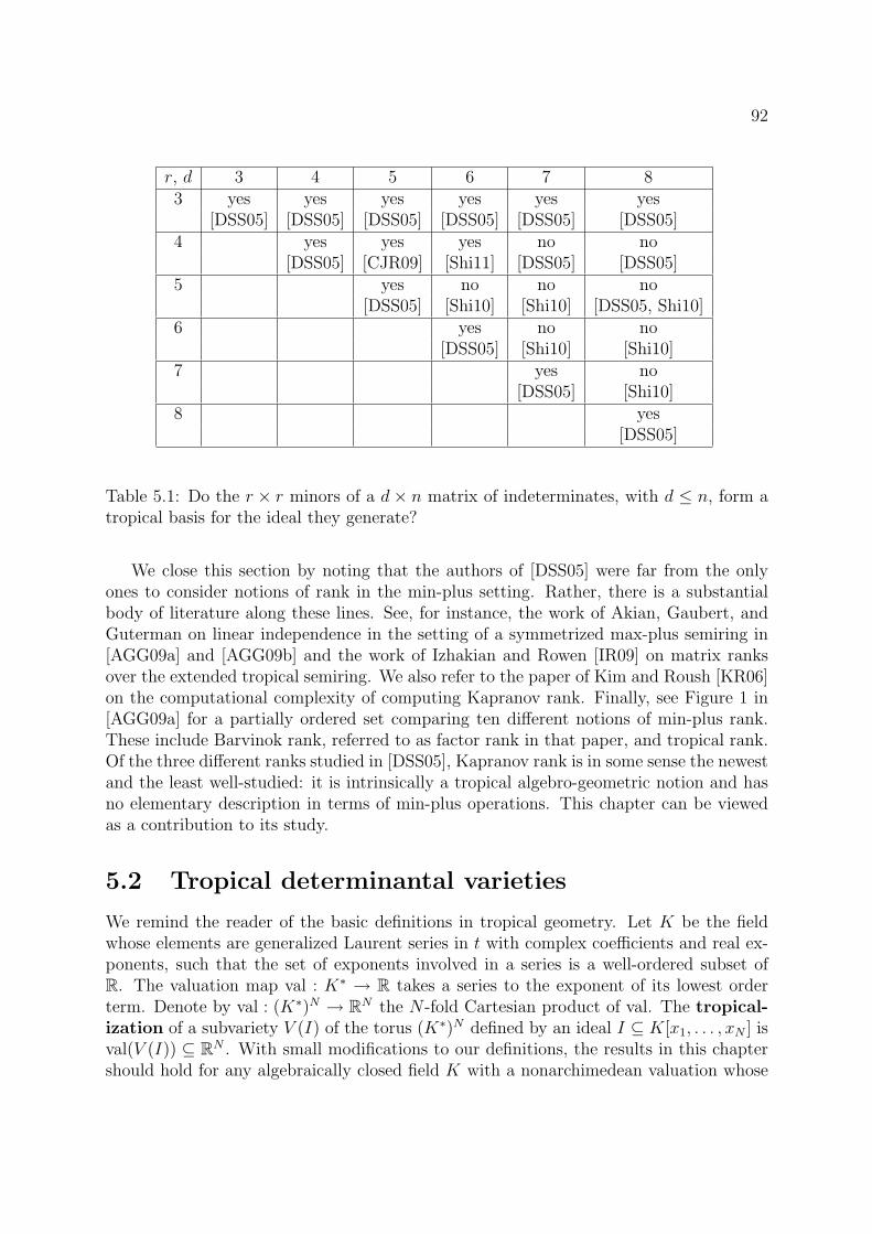
92

r, d 3 4 5 6 7 83 yes yes yes yes yes yes

[DSS05] [DSS05] [DSS05] [DSS05] [DSS05] [DSS05]4 yes yes yes no no

[DSS05] [CJR09] [Shi11] [DSS05] [DSS05]5 yes no no no

[DSS05] [Shi10] [Shi10] [DSS05, Shi10]6 yes no no

[DSS05] [Shi10] [Shi10]7 yes no

[DSS05] [Shi10]8 yes

[DSS05]

Table 5.1: Do the r × r minors of a d× n matrix of indeterminates, with d ≤ n, form atropical basis for the ideal they generate?

We close this section by noting that the authors of [DSS05] were far from the onlyones to consider notions of rank in the min-plus setting. Rather, there is a substantialbody of literature along these lines. See, for instance, the work of Akian, Gaubert, andGuterman on linear independence in the setting of a symmetrized max-plus semiring in[AGG09a] and [AGG09b] and the work of Izhakian and Rowen [IR09] on matrix ranksover the extended tropical semiring. We also refer to the paper of Kim and Roush [KR06]on the computational complexity of computing Kapranov rank. Finally, see Figure 1 in[AGG09a] for a partially ordered set comparing ten different notions of min-plus rank.These include Barvinok rank, referred to as factor rank in that paper, and tropical rank.Of the three different ranks studied in [DSS05], Kapranov rank is in some sense the newestand the least well-studied: it is intrinsically a tropical algebro-geometric notion and hasno elementary description in terms of min-plus operations. This chapter can be viewedas a contribution to its study.

5.2 Tropical determinantal varieties

We remind the reader of the basic definitions in tropical geometry. Let K be the fieldwhose elements are generalized Laurent series in t with complex coefficients and real ex-ponents, such that the set of exponents involved in a series is a well-ordered subset ofR. The valuation map val : K∗ → R takes a series to the exponent of its lowest orderterm. Denote by val : (K∗)N → RN the N -fold Cartesian product of val. The tropical-

ization of a subvariety V (I) of the torus (K∗)N defined by an ideal I ⊆ K[x1, . . . , xN ] isval(V (I)) ⊆ RN . With small modifications to our definitions, the results in this chaptershould hold for any algebraically closed field K with a nonarchimedean valuation whose

93

image is dense in the reals; these assumptions are necessary to accomodate our use ofthe Fundamental Theorem of Tropical Geometry, the characterization of Kapranov rankin terms of tropicalized linear spaces in [DSS05, Theorem 3.3], and the results on stableintersections [Spe05b, Proposition 4.4.1, Theorem 4.4.6, Proposition 4.5.3].

For ω ∈ RN , the ω-degree of a monomial cxa = cxa11 · · ·xaN

N is val(c) + 〈ω, a〉. Theinitial form inω(f) ∈ C[x1, . . . , xN ] of a polynomial f ∈ K[x1, . . . ,xN ] with respect to ω is the sum of terms of the form γtbxa (γ ∈ C) in f with minimalω-degree, but with 1 substituted for t. Define the initial ideal

inω(I) := 〈inω(f) : f ∈ I〉 ⊆ C[x1, . . . , xN ].

The Fundamental Theorem of Tropical Geometry, variously attributed to Draisma, Kapra-nov, Speyer-Sturmfels (see [Dra08],[SS04]), says that val(V (I)) equals the tropical va-

riety T (I), with

T (I) := {ω ∈ RN : inω(I) does not contain a monomial}.

The Grobner complex Σ(I) of a homogeneous ideal I, see [MS10], is the polyhedralcomplex consisting of all polyhedra

Cω(I) := {ω′ ∈ RN : inω(I) = inω′(I)},

where ω runs through RN , and the closure is taken in the usual Euclidean topology ofRN . It is clear that the tropical variety T (I) is the support of a subcomplex of Σ(I), andwe shall not distinguish between T (I) and this subcomplex.

By the linear span of a polyhedron P ⊆ RN we mean the R-span of P − P :={p− p′ : p, p′ ∈ P}. The intersection of the linear spans of all the polyhedra in a complexis called the lineality space of the complex. A complex is invariant under translationby elements of its lineality space. Since I is homogeneous, the lineality space of Σ(I)contains the (1, . . . , 1) vector and it makes sense to consider T (I) in the tropical torus

TPN−1 := RN/ ∼, where we quotient out by coordinate-wise tropical multiplication by aconstant.

If I is a principal ideal 〈f〉, where f =∑

i cixai with ci ∈ K∗, the tropical variety is

called a hypersurface. It consists of all ω ∈ RN such that the minimum

⊕

i

val(ci) ⊙ 〈ω, ai〉 (5.2)

is attained at least twice.In the special case where I is defined by polynomials with coefficients in C, the complex

Σ(I) is a fan. In this chapter, we study two kinds of tropical varieties: those defined bylinear ideals in K[x1, . . . , xN ], which yield polyhedral complexes; and those which aresets of matrices of Kapranov rank at most r, and are therefore polyhedral fans (sincetheir ideals are defined over C). In the latter case, we use the terms Grobner fan andGrobner cones for Σ(I) and its cones.

94

Definition 5.2.1. Let A,B be polyhedral fans. The common refinement of A and Bis the fan

A ∧B := {a ∩ b : a is a cone of A and b is a cone of B}.

The support of a fan A is the set of points p ∈ Rn such that p lies in some cone of A.Note that the support of A ∧ B is the intersection of the support of A and the supportof B.

Definition 5.2.2. Given a set F = {f1, . . . , fm} ⊆ K[x1, . . . , xN ], its tropical prevari-

ety is the intersection ⋂

i

T (〈fi〉).

The set F is a tropical basis if its prevariety equals T (〈f1, . . . , fm〉). If each T (〈fi〉) is afan, then the prevariety can be regarded as their common refinement and hence is a fan.

We can now give precise definitions of rank.

Definition 5.2.3. Let Fdnr ⊆ K[x1, . . . , xdn] be the set of (r+ 1)× (r+ 1) minors of the

d× n matrix {xij}. Let Jdnr = 〈f : f ∈ Fdnr 〉, and A ∈ Rd×n.

• A has tropical rank at most r if A ∈⋂f∈Fdn

rT (〈f〉).

• A has Kapranov rank at most r if A ∈ T (Jdnr ).

Equivalently, by the Fundamental Theorem, a matrix A has Kapranov rank at mostr if it has a lift A over K of rank at most r. By a lift we mean a matrix A such thatval(A) = A.

Example 5.2.4. Let f ∈ K[x11, . . . , x33] be the 3 × 3 determinant,

A =

0 1 21 1 10 1 1

and A =

1 t t2

2t 3t 5t1 + 2t 4t 5t+ t2

.

The tropical hypersurface T (〈f〉) contains A since (5.2) attains its minimum three times.Hence, A has tropical rank at most 2. Equivalently, inA(f) = x11x22x33 − x11x23x32 +x12x23x31 is not a monomial. The tropical rank is not less than 2, since inA(x11x22 −x12x21) = x11x22. Thus the tropical rank is 2. To argue about the Kapranov rank, weconsider the lift A ∈ K3×3 above. The classical rank of A is 2. By the fundamentaltheorem, or since inA(J33

2 ) is monomial-free, A has Kapranov rank at most 2. Since itsKapranov rank is at least its tropical rank, it is equal to 2. ⋄

95

5.3 The 4 × 4 minors of a 5 × n matrix are a tropical

basis

The goal of this section is to prove our main theorem, Theorem 5.1.2. For an alternativeproof, see [Rub07]. For a computational proof of the 5 × 5 case, see [CJR09].

The idea of the proof presented here is as follows.. Given a 5 × n matrix of tropicalrank at most 3, we will produce five tropical hyperplanes, each containing the n columnvectors of A. Then, we will argue that some pair of these hyperplanes must contain thesen points in their stable intersection and conclude that the Kapranov rank is at most3. The central argument is an analysis of the possible combinatorial types of the point-hyperplane incidences. We begin with some definitions. In the following the ambientspace will be TPd−1 with d general, but we will later specialize to the case where d is thenumber of rows of the matrix, in our case d = 5.

Definition 5.3.1. Let H be the tropical hyperplane in TPd−1 corresponding to the trop-ical polynomial h1⊙x1⊕· · ·⊕hd⊙xd; that is, H is the set of points (x1, . . . , xd) at whichh1 ⊙ x1 ⊕ · · · ⊕ hd ⊙ xd attains its minimum at least twice, and we write

H = T (h1 ⊙ x1 ⊕ · · · ⊕ hd ⊙ xd).

Let w = (w1, . . . , wd) be a point in TPd−1.Then the type of w with respect to H, denoted typeH w, is the subset of [d] of those

indices at which the minimum of h1 ⊙ w1, . . . , hd ⊙ wd is attained. Thus, |typeH w| ≥ 2if and only if w ∈ H.

Note that our definition of type is similar to the definition by Ardila and Develin in[AD09] which gives rise to tropical oriented matroids. The only difference is that ourtypes are taken with respect to a single hyperplane instead of a hyperplane arrangement.

Types have a natural geometric interpretation, as follows. A tropical hyperplane Hdivides TPd−1 into d sectors: the ith closed sector consists of those points w for which theminimum when the tropical function corresponding to H is evaluated at w is attained atcoordinate i. The type of a point records precisely in which closed sectors it lies. Figure5.1 illustrates the case of a tropical line in TP2.

Recall that a tropicalized linear space is the tropicalization of a classical linearvariety in K[x1, . . . , xd]. If the linear space is a classical hyperplane, then we just call itstropicalization a tropical hyperplane as in Definition 5.3.1. The stable intersection

of two tropical linear spaces L and L′ is

limv→0L ∩ (L′ + v)

where v approaches 0 along a ray whose direction lies in an open dense subset of Sn−1 (see[Spe08, p. 1545] for a discussion on the topology on the set of the polyhedral complexes).It is itself a tropicalized linear space, see [Spe05b, Proposition 4.4.1, Theorem 4.4.6]. Toclarify, a point w lies in the stable intersection of L and L′ if and only if for all ε > 0,there exists δ > 0 and an open dense subset A ⊆ Sn−1 such that for each v ∈ Rn with

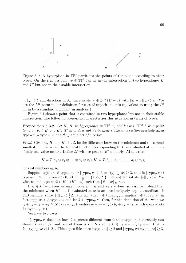
96

123

12

13

3

2

1

H H′

w23

Figure 5.1: A hyperplane in TP2 partitions the points of the plane according to theirtypes. On the right, a point w ∈ TP2 can lie in the intersection of two hyperplanes Hand H ′ but not in their stable intersection.

‖v‖∞ < δ and direction in A, there exists w ∈ L ∩ (L′ + v) with ‖w − w‖∞ < ε. (Weuse the L∞ norm in our definition for ease of exposition; it is equivalent to using the L2

norm by a standard argument in analysis.)Figure 5.1 shows a point that is contained in two hyperplanes but not in their stable

intersection. The following proposition characterizes this situation in terms of types.

Proposition 5.3.2. Let H, H ′ be hyperplanes in TPd−1, and let w ∈ TPd−1 be a pointlying on both H and H ′. Then w does not lie in their stable intersection precisely whentypeH w = typeH′ w and they are a set of size two.

Proof. Given w, H, and H ′, let ∆ be the difference between the minimum and the secondsmallest number when the tropical function corresponding to H is evaluated at w, or ∞if only one value occurs. Define ∆′ with respect to H ′ similarly. Also, write

H = T (a1 ⊙ x1 ⊕ · · · ⊕ ad ⊙ xd), H′ = T (b1 ⊙ x1 ⊕ · · · ⊕ bd ⊙ xd),

for real numbers ai, bi.Suppose typeH w 6= typeH′ w or | typeH w| ≥ 3 or | typeH′ w| ≥ 3, that is | typeH w ∪

typeH′ w| ≥ 3. Given ε > 0, let δ = 12min{ε,∆,∆′}. Let v ∈ Rn satisfy ‖v‖∞ < δ. We

wish to find a point w ∈ H ∩ (H ′ + v) such that ‖w − w‖∞ < ε.If w ∈ H ′ + v then we may choose w = w and we are done, so assume instead that

the minimum when H ′ + v is evaluated at w is achieved uniquely, say at coordinate i.Furthermore, since ‖v‖∞ < 1

2∆′, the fact that i ∈ typeH′+v w implies i ∈ typeH′ w (in

fact suppose i 6∈ typeH′ w and let k ∈ typeH′ w, then, for the definition of ∆′, we havebi +wi − bk +wk ≥ ∆′ > vi − vk, therefore bi +wi − vi > bk +wk − vk, which contradictsi ∈ typeH′+v w).

We have two cases:

1) typeH w does not have 2 elements different from i; thus typeH w has exactly twoelements, say 1, 2, and one of them is i. Pick some k ∈ typeH′ w \ typeH w that isk ∈ typeH′ w \ {1, 2}. This is possible since | typeH′ w| ≥ 2 and | typeH w∪ typeH′ w| ≥ 3.

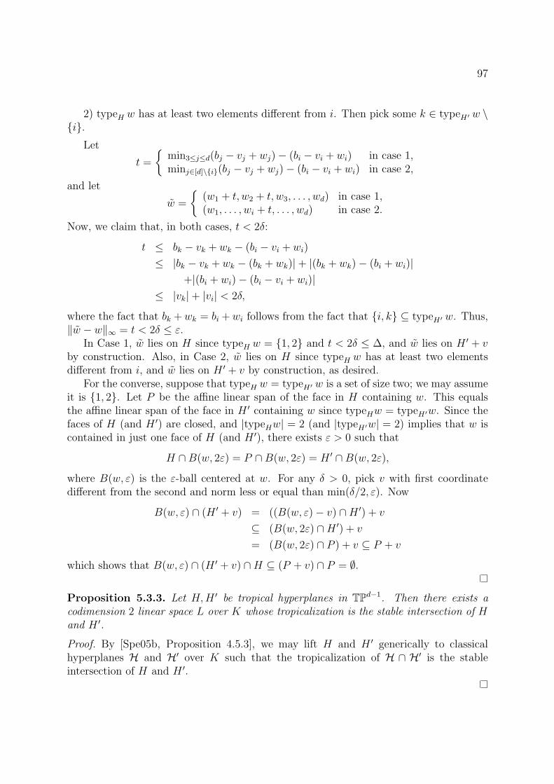
97

2) typeH w has at least two elements different from i. Then pick some k ∈ typeH′ w \{i}.

Let

t =

{min3≤j≤d(bj − vj + wj) − (bi − vi + wi) in case 1,minj∈[d]\{i}(bj − vj + wj) − (bi − vi + wi) in case 2,

and let

w =

{(w1 + t, w2 + t, w3, . . . , wd) in case 1,(w1, . . . , wi + t, . . . , wd) in case 2.

Now, we claim that, in both cases, t < 2δ:

t ≤ bk − vk + wk − (bi − vi + wi)

≤ |bk − vk + wk − (bk + wk)| + |(bk + wk) − (bi + wi)|

+|(bi + wi) − (bi − vi + wi)|

≤ |vk| + |vi| < 2δ,

where the fact that bk +wk = bi +wi follows from the fact that {i, k} ⊆ typeH′ w. Thus,‖w − w‖∞ = t < 2δ ≤ ε.

In Case 1, w lies on H since typeH w = {1, 2} and t < 2δ ≤ ∆, and w lies on H ′ + vby construction. Also, in Case 2, w lies on H since typeH w has at least two elementsdifferent from i, and w lies on H ′ + v by construction, as desired.

For the converse, suppose that typeH w = typeH′ w is a set of size two; we may assumeit is {1, 2}. Let P be the affine linear span of the face in H containing w. This equalsthe affine linear span of the face in H ′ containing w since typeHw = typeH′w. Since thefaces of H (and H ′) are closed, and |typeHw| = 2 (and |typeH′w| = 2) implies that w iscontained in just one face of H (and H ′), there exists ε > 0 such that

H ∩B(w, 2ε) = P ∩B(w, 2ε) = H ′ ∩B(w, 2ε),

where B(w, ε) is the ε-ball centered at w. For any δ > 0, pick v with first coordinatedifferent from the second and norm less or equal than min(δ/2, ε). Now

B(w, ε) ∩ (H ′ + v) = ((B(w, ε) − v) ∩H ′) + v

⊆ (B(w, 2ε) ∩H ′) + v

= (B(w, 2ε) ∩ P ) + v ⊆ P + v

which shows that B(w, ε) ∩ (H ′ + v) ∩H ⊆ (P + v) ∩ P = ∅.

Proposition 5.3.3. Let H,H ′ be tropical hyperplanes in TPd−1. Then there exists acodimension 2 linear space L over K whose tropicalization is the stable intersection of Hand H ′.

Proof. By [Spe05b, Proposition 4.5.3], we may lift H and H ′ generically to classicalhyperplanes H and H′ over K such that the tropicalization of H ∩ H′ is the stableintersection of H and H ′.

98

Now letW be a set of points in TPd−1, and let i ∈ {1, . . . , d}. We say that a hyperplaneH that contains each point in W is an i-coordinate hyperplane for W if typeH w doesnot contain i for any w ∈ W . That is, no point in W lies in the ith closed sector of H.

Next, suppose w is a point contained in two hyperplanes H and H ′ but not in theirstable intersection. Then, by Proposition 5.3.3, w has type {a, b} with respect to both Hand H ′, for some a and b. Then we say that w is a witness of type ab to the nonstableintersection of H and H ′. In the case that H and H ′ are k- and l-coordinate hyperplanes,respectively, for a set of points W containg w, we note that the sets {a, b} and {k, l} mustbe disjoint.

We are now ready to state a proposition which will serve as the combinatorial heartof our proof of Theorem 5.1.2.

Proposition 5.3.4. Let W = {w1, . . . , wn} be a subset of points in TP4, and for eachi with 1 ≤ i ≤ 5, let Hi be a hyperplane containing each point in W such that Hi is ani-coordinate hyperplane for W . Suppose further that for every pair of hyperplanes Hi andHj, the intersection Hi∩Hj is not the stable intersection of Hi and Hj and some ws ∈ Wwitnesses this nonstable intersection.

Let i, j, k, l,m be distinct elements in {1, 2, 3, 4, 5}. Suppose Hi and Hj have a witnessin W of type kl. Then any witness in W for Hi and Hk has type lm.

Proposition 5.3.4 follows from the following two lemmas, whose proofs we postponeto the end of the section.

Lemma 5.3.5. Let W = {w1, . . . , wn}, H1, . . . , H5 be as in the first paragraph of Propo-sition 5.3.4. Let i, j, k, l be distinct elements in {1, . . . , 5}, and assume without loss ofgenerality that Hi and Hj have a witness in W of type kl. Then any witness in W forHi and Hk must be of type containing l.

Lemma 5.3.6. Let W = {w1, . . . , wn}, H1, . . . , H5 be as in the first paragraph of Propo-sition 5.3.4. Let i, j, k, l be distinct elements in {1, . . . , 5}. Then it is not possible thatHi and Hk have a witness in W of type jl and that Hi and Hj have a witness in W oftype kl.

Proof of Proposition 5.3.4. Hi and Hk have some witness to their nonstable intersection;it must be of type jl, jm, or lm. But it is not of type jm by Lemma 5.3.5, and it is notof type jl by Lemma 5.3.6.

Before proving the lemmas, we first prove that Proposition 5.3.4 implies the mainresult.

Proof of Theorem 5.1.2. Fix n ≥ 4; let A be a 5×n real matrix, and letW = {w1, . . . , wn}be the set of its column vectors. Suppose that the tropical rank of A is ≤ 3. We wish toshow that the Kapranov rank is ≤ 3, or equivalently, that there exists a 3-dimensionalsubspace in K5 whose tropicalization contains each point w1, . . . , wn.

99

Let A′ be the 4× n matrix obtained by deleting the first row of A. Then the tropicalrank of A′ is ≤ 3, so by [DSS05, Theorem 5.5, 6.5], the Kapranov rank of A′ is ≤ 3, sothe columns of A′ lie on some tropical hyperplane, say

T (h12 ⊙ x2 ⊕ h13 ⊙ x3 ⊕ h14 ⊙ x4 ⊕ h15 ⊙ x5).

Then, for N sufficiently large,

H1 := T (N ⊙ x1 ⊕ h12 ⊙ x2 ⊕ h13 ⊙ x3 ⊕ h14 ⊙ x4 ⊕ h15 ⊙ x5)

is a hyperplane containing the columns of A, indeed a 1-coordinate hyperplane, wherenone of w1, . . . , wn has type containing 1.

Similarly, we may choose H2, H3, H4, H5 to be 2, 3, 4, 5-coordinate hyperplanes, re-spectively, for the points w1, . . . , wn.

We claim that for some i, j with 1 ≤ i < j ≤ 5, Hi and Hj contain each w1, . . . , wn intheir stable intersection. If so, we are done by Proposition 5.3.3.

Suppose, then, that the claim is not true, so that for every i, j with 1 ≤ i < j ≤ 5, somepoint in W witnesses the nonstable intersection of Hi and Hj. We derive a contradictionas follows.

By symmetry, we may assume that H1 and H2 have a witness of type 34. We nowapply Proposition 5.3.4 four times to get a contradiction. First, H1 and H3 have a witnessin W to their nonstable intersection by assumption; it is of type 45 by Proposition 5.3.4.Similarly, H1 and H4 have a witness in W of type 35. Applying Proposition 5.3.4 to thesetwo facts, we get that any witness in W for H1 and H5 must have type 24, and similarly,that any witness in W for H1 and H5 must have type 23. Since H1 and H5 do have awitness in W , by assumption, this is a contradiction.

Proof of Lemma 5.3.5. By symmetry, assume i = 1, j = 2, k = 4, l = 5. Suppose H1 andH2 have a witness of type 45, and that H1 and H4 have a witness of type not containing5 – that is, we assume that H1 and H4 have a witness of type 23. We wish to derive acontradiction.

For each s with 1 ≤ s ≤ 5, write

Hs = T (hs1 ⊙ x1 ⊕ · · · ⊕ hs5 ⊙ x5),with hsr ∈ R.

By translating each hyperplane and each point, we may assume that

H1 = T (0 ⊙ x1 ⊕ · · · ⊕ 0 ⊙ x5),

and for each s with 2 ≤ s ≤ 5, we may assume, by tropically scaling the coefficients ofHs, that hs1 = 0. Furthermore, since H1 and H2 have a witness of type 45, and h14 = h15,it follows that h24 = h25. Similarly, h42 = h43. Summarizing, we have

H1 = T (0x1 ⊕ 0x2 ⊕ 0x3 ⊕ 0x4 ⊕ 0x5),

H2 = T (0x1 ⊕ ex2 ⊕ bx3 ⊕ ax4 ⊕ ax5),

H4 = T (0x1 ⊕ cx2 ⊕ cx3 ⊕ fx4 ⊕ dx5),

100

with a, b, c, d, e, f ∈ R. By symmetry (i.e. switching 2 with 4 and 3 with 5), we mayassume a ≤ c.

Now, we claim b > a. Indeed, let γ = (γ1, γ2, γ3, γ4, γ5) be a witness of type 23 forH1 and H4. Since typeH1

(γ) = 23, we have that the minimum of {γ1, γ2, γ3, γ4, γ5} isattained twice, in fact, precisely at γ2 and γ3. Tropically rescaling, we may assume thatγ2 = γ3 = 0 and that γ1, γ4, γ5 > 0. Since typeH4

(γ) = 23, we have that min(γ1, c+γ2, c+γ3, f + γ4, d + γ5) is attained precisely at c + γ2 = c + γ3 = c, so γ1 > c. Finally, sinceγ ∈ H2, and H2 is a 2-coordinate hyperplane, we have that min(γ1, b+ γ3, a+ γ4, a+ γ5)is achieved twice. Since γ1 > c ≥ a, γ3 = 0, γ4, γ5 > 0, this is only possible if b > a.

Next, we claim d > a. The proof is similar. Let χ = (χ1, . . . , χ5) ∈ TP4 be a witnessof type 45 for H1 and H2. Using that typeH1

χ = typeH2χ = {4, 5} and tropically

rescaling, we have χ1 > a, χ2 > 0, χ3 > 0, χ4 = χ5 = 0. Together with a ≤ cthis implies c + χ2, c + χ3 > a. But χ ∈ H4 and H4 is a 4-coordinate hyperplane, somin(χ1, c + χ2, c + χ3, d + χ5) is attained twice, and since χ1, c + χ2, c + χ3 are all > aand χ5 = 0, we have d > a.

Now, H2 and H4 have some witness of nonstable intersection, say ψ = (ψ1, ψ2, ψ3, ψ4,ψ5) ∈ TP4, where ψ is a witness of type 13, 15, or 35. Since h21 = h41 = 0, buth25 = a 6= d = h45, it is not type 15, so it is of type 13 or 35.

Suppose ψ is of type 35, so typeH2ψ = typeH4

ψ = {3, 5}. Then, rescaling, we mayassume ψ3 = a, ψ5 = b, ψ2 > a, and ψ4 > b. But we showed b > a, so min(ψ2, ψ3, ψ4, ψ5)is attained uniquely, contradicting that ψ ∈ H1 and H1 is a 1-coordinate hyperplane.

So ψ must be a witness of type 13 for H2 and H4. Since h21 = h41 = 0, we haveh23 = h43, that is, b = c. Furthermore, using typeH2

ψ = typeH4ψ = {1, 3}, and rescaling

ψ, we may assume that ψ1 = b, ψ2 > 0, ψ3 = 0, ψ4 > b − a, ψ5 > b − a. But sinceb − a > 0 and H1 is a 1-coordinate hyperplane, ψ /∈ H1, contradiction. This provesLemma 5.3.5.

Proof of Lemma 5.3.6. By symmetry, we may assume i = 1, j = 4, k = 3, l = 2, and wesuppose for a contradiction that H1 and H3 have a witness, γ, of type 24, and H1 andH4 have a witness, χ, of type 23. We may assume, by translating and rescaling, that

H1 = T (0x1 ⊕ 0x2 ⊕ 0x3 ⊕ 0x4 ⊕ 0x5),

H3 = T (0x1 ⊕ ax2 ⊕ ex3 ⊕ ax4 ⊕ bx5),

H4 = T (0x1 ⊕ cx2 ⊕ cx3 ⊕ fx4 ⊕ dx5),

for some a, b, c, d, e, f ∈ R. Then, rescaling, we may assume that γ = (γ1, 0, γ3, 0, γ5)where γ1 > a, γ3 > 0, and γ5 > a−b. Similarly, we may assume that χ = (χ1, 0, 0, χ4, χ5),where χ1 > c, χ4 > 0, and χ5 > c− d.

Now, by hypothesis, H3 and H4 have some witness ψ to their nonstable intersection;its type must be 12, 15, or 25, since types containing 3 or 4 may not occur.

Suppose it is type 12. Then a = c. That γ lies on H4 implies that min(γ1, c, c+γ3, d+γ5) is attained twice; since γ1 > a = c and c+γ3 > c, we have c = d+γ5. Since γ5 > a−b,we have c > d+ a− b, so b > d. Symmetrically, χ ∈ H3 implies min(χ1, a, a+ χ4, b+ χ5)

101

is achieved twice; since χ1 > c = a, a + χ4 > a and b + χ5 > b + c − d = a + b − d, itfollows that d > b, contradiction.

Next, suppose ψ is a witness for H3 and H4 of type 15. Then b = d. Then γ ∈ H4

implies that min(γ1, c, c+ γ3, d+ γ5) is achieved twice; since γ1 > a, γ3 > 0 and d+ γ5 >d + a − b = a, it follows that c > a (otherwise the minimum is achieved uniquely at c).Symmetrically, χ ∈ H3 implies min(χ1, a, a + χ4, b + χ5) is achieved twice; since χ1 > c,a+ χ4 > a and b+ χ5 > b+ c− d = c, it follows that a > c, contradiction.

Finally, suppose ψ is a witness of type 25. Then a+d = b+c, and γ ∈ H4 implies thatmin(γ1, c, c+γ3, d+γ5) is attained twice; since γ1 > a, c+γ3 > c, and d+γ5 > d+a−b = c,we have c > a. Symmetrically, χ ∈ H3 implies min(χ1, a, a+χ4, b+χ5) is achieved twice;since χ1 > c, a + χ4 > a and b + χ5 > b + c − d = a, it follows that a > c. This is acontradiction and proves Lemma 5.3.6.

102

Bibliography

[AGG09a] M. Akian, S. Gaubert, A. Guterman, Linear independence over tropical semir-ings and beyond, Contemporary Mathematics 495 (2009) 138.

[AGG09b] M. Akian, S. Gaubert, A. Guterman, Tropical polyhedra are equivalent tomean payoff games, to appear in International Journal on Algebra and Computations,preprint available at arXiv:0912.2462.

[ABC11] O. Amini, L. Caporaso, Riemann-Roch theory for weighted graphs and tropicalcurves, arXiv:1112.5134.

[AD09] F. Ardila, M. Develin, Tropical hyperplane arrangements and oriented matroids,Mathematische Zeitschrift 262 (4) (2009) 795–816.

[AD09] M. Artebani and I. Dolgachev, The Hesse pencil of plane cubic curves, Enseign.Math. (2) 55 (2009) 235–273.

[AMRT75] A. Ash, D. Mumford, M. Rapoport, Y. Tai, Smooth compactification of lo-cally symmetric varieties, Lie Groups: History, Frontiers and Applications, Vol. IV,Math. Sci. Press, Brookline, Mass., 1975.

[Bak08] M. Baker, Specialization of linear systems from curves to graphs, Algebra Num-ber Theory 2 (2008), no. 6, 613–653.

[BF11] M. Baker, X. Faber, Metric properties of the tropical Abel-Jacobi map, Journalof Algebraic Combinatorics 33, no. 3 (2011), 349–381.

[BN07] M. Baker, S. Norine, Riemann-Roch and Abel-Jacobi theory on a finite graph,Adv. Math. 215 (2007), no. 2, 766-788.

[BN09] M. Baker, S. Norine, Harmonic morphisms and hyperelliptic graphs, InternationalMath. Research Notices 15 (2009), 2914–2955.

[BPR11] M. Baker, S. Payne, J. Rabinoff, Nonarchimedean geometry, tropicalization,and metrics on curves, arXiv:1104.0320.

[Bal70] A. T. Balaban, Rev. Roumaine Chim. 15 (1970), 463.

103

[Bal76] A. T. Balaban, Enumeration of Cyclic Graphs, pp. 63-105 of A. T. Balaban, ed.,Chemical Applications of Graph Theory, Ac. Press, 1976.

[Ber90] V. Berkovich, Spectral theory and analytic geometry over non-Archimedeanfields, Mathematical Surveys and Monographs, 33, American Mathematical Society,Providence, RI, 1990.

[BG84] R. Bieri, J. R. J. Groves, The geometry of the set of characters induced byvaluations. J. Reine Angew. Math. 347 (1984) 168–195.

[BCS05] L. Borisov, L. Chen, G. Smith. The orbifold Chow ring of toric Deligne-Mumfordstacks, J. Amer. Math. Soc. 18 (2005), no. 1, 193–215.

[BJSST07] T. Bogart, A. N. Jensen, D. Speyer, B. Sturmfels, R. R. Thomas, Computingtropical varieties, J. Symbolic Comput. 42 (1-2) (2007) 54–73.

[Bra93] T. Brady, The integral cohomology of Out+(F3), J. Pure and Applied Algebra87 (1993) 123-167.

[BMV11] S. Brannetti, M. Melo, F. Viviani, On the tropical Torelli map, Advances inMathematics 226 (2011) 2546–2586.

[BM11] E. Brugalle and L. L. de Medrano, Inflection points of real and tropical planecurves, preprint available at arXiv:1102.2478.

[Buc10] A. Buchholz, Tropicalization of Linear Isomorphisms on Plane Elliptic Curves,Diplomarbeit, University of Gottingen, Germany, April 2010.

[Cap10] L. Caporaso, Geometry of tropical moduli spaces and linkage of graphs, Journalof Combinatorial Theory, Series A 119 (2012) 579–598.

[Cap11a] L. Caporaso, Algebraic and tropical curves: comparing their moduli spaces, toappear in Handbook of Moduli, edited by G. Farkas and I. Morrison, 2011.

[Cap11b] L. Caporaso, Algebraic and combinatorial Brill-Noether theory, to appearin Compact moduli spaces and vector bundles, V. Alexeev, E. Izadi, A. Gibney,J. Kollar, E. Loojenga, eds., Contemporary Mathematics 564, American Mathemat-ical Society, Providence, RI, 2012, preprint available at arXiv:1106.1140v1.

[CV10] L. Caporaso, F. Viviani, Torelli theorem for graphs and tropical curves, DukeMath. Journal 153 (2010) 129-171.

[Cay75] A. Cayley, On the analytical forms called trees, with application to the theoryof chemical combinations, Reports British Assoc. Advance. Sci. 45 (1875), 257-305.

[Cha11a] M. Chan, Combinatorics of the tropical Torelli map, to appear in AlgebraNumber Theory, preprint available at arXiv:1012.4539v2.

104

[Cha11b] M. Chan, Tropical hyperelliptic curves, to appear in Journal of Algebraic Com-binatorics, preprint available at arXiv:1110.0273.

[CJR09] M. Chan, A. N. Jensen, E. Rubei, The 4 × 4 minors of a 5 × n matrix are atropical basis, Linear Algebra and its Applications 435 (2011) 1598–1611.

[CS12] M. Chan, B. Sturmfels, Elliptic curves in honeycomb form, preprint available atarXiv:1203.2356.

[CDPR10] F. Cools, J. Draisma, S. Payne, and E. Robeva, A tropical proof of the Brill-Noether Theorem, to appear in Advances in Mathematics, preprint available atarXiv:1001.2774v2.

[CV84] M. Culler, K. Vogtmann, Moduli of graphs and automorphisms of free groups,Invent. Math., 84 (1) (1986) 91-119.

[DSS05] M. Develin, F. Santos, B. Sturmfels, On the rank of a tropical matrix, In “Dis-crete and Computational Geometry” (E. Goodman, J. Pach and E. Welzl, eds),MSRI Publications, Cambridge University Press (2005).

[Dra08] J. Draisma, A tropical approach to secant dimensions, J. Pure Appl. Algebra 212(2) (2008) 349-363.

[Eng02a] P. Engel, The contraction types of parallelohedra in E5, Acta Cryst. A 56(2002), 491–496.

[Eng02b] P. Engel, V. Grishukhin, There are exactly 222 L-types of primitive five-dimensional lattices, European Journal of Combinatorics 23 (2002), 275–279.

[GK08] A. Gathmann and M. Kerber, A Riemann-Roch theorem in tropical geometry,Math. Z. 259 (2008), no. 1, 217–230.

[GKM09] A. Gathmann, M. Kerber, H. Markwig, Tropical fans and the moduli spaces oftropical curves, Compos. Math. 145 (2009), no. 1, 173–195.

[GH80] P. Griffiths and J. Harris, On the variety of special linear systems on a generalalgebraic curve, Duke Math. J. 47 (1980), no. 1, 233–272.

[Ger82] L. Gerritzen, Die Jacobi-Abbildung uber dem Raum der Mumfordkurven,Math. Ann. 261 (1982), no. 1, 81–100.

[Gru09] S. Grushevsky, The Schottky problem, Proceedings of “Classical algebraic ge-ometry today” workshop (MSRI, January 2009), to appear.

[HMY09] C. Haase, G. Musiker, and J. Yu, Linear systems on tropical curves, to appearin Math. Z, preprint available at arXiv:0909.3685.

[Har77] R. Hartshorne, Algebraic Geometry, Springer Verlag, New York, 2006.

105

[Hel11] P.A. Helminck, Tropical Elliptic Curves and j-Invariants, Bachelor’s Thesis,University of Groningen, The Netherlands, August 2011.

[IR09] Z. Izhakian, L. Rowen, The tropical rank of a tropical matrix, Comm. Algebra 37(11) (2009) 3912-3927.

[Jen] A. N. Jensen, Gfan, a software system for Grobner fans and tropical varieties,available at http://home.imf.au.dk/jensen/software/gfan/gfan.html.

[Jor77] C. Jordan, Memoire sur les equations differentielles lineaires a integralealgebrique, Journal fur Reine und Angew. Math. 84 (1877) 89–215.

[KMM08] E. Katz, H. Markwig and T. Markwig, The j-invariant of a plane tropical cubic,J. Algebra 320 (2008) 3832–3848.

[KR06] K. H. Kim, F. W. Roush, Kapranov vs. tropical rank, Proc. Amer. Math.Soc. 134 (9) (2006) 2487–2494.

[LPP11] C. M. Lim, S. Payne, N. Potashnik, A note on Brill-Noether theory and rank de-termining sets for metric graphs, to appear in International Math. Research Notices,preprint available at arXiv:1106.5519v1.

[MS10] D. Maclagan, B. Sturmfels, Introduction to Tropical Geometry, book manuscript,2010, available athttp://www.warwick.ac.uk/staff/D.Maclagan/papers/TropicalBook.pdf.

[MP] S. Maggiolo, N. Pagani, Generating stable modular graphs, Journal of SymbolicComputation 46 (10) (2011), 1087–1097.

[Mik06a] G. Mikhalkin, Moduli spaces of rational tropical curves, Proceedings of GokovaGeometry-Topology Conference 2006, 39–51, Gokova Geometry/Topology Confer-ence (GGT), Gokova, 2007.

[Mik06b] G. Mikhalkin, Tropical geometry and its applications, International Congressof Mathematicians. Vol. II, 827–852, Eur. Math. Soc., Zurich, 2006.

[MZ07] G. Mikhalkin and I. Zharkov, Tropical curves, their Jacobians and theta func-tions, Contemporary Mathematics 465, Proceedings of the International Conferenceon Curves and Abelian Varieties in honor of Roy Smith’s 65th birthday (2007),203–231.

[Nob11] A. Nobe, The group law on the tropical Hesse pencil, arXiv:1111.0131.

[OEIS] The On-Line Encyclopedia of Integer Sequences, published electronically athttp://oeis.org, 2011.

[Oxl92] J. Oxley, Matroid Theory, Oxford Univ. Press, New York, 1992.

http://home.imf.au.dk/jensen/software/gfan/gfan.html

106

[Pay09] S. Payne, Analytification is the limit of all tropicalizations, Math. Res. Lett. 16(2009), no. 3, 543–556.

[RS99] E. M. Rains and N. J. A. Sloane, On Cayley’s Enumeration of Alkanes (or 4-ValentTrees), J. Integer Sequences, Vol. 2 (1999), Article 99.1.1.

[Roq70] P. Roquette, Analytic Theory of Elliptic Functions over Local Fields, HamburgerMathematische Einzelschriften, Heft 1, Vandenhoeck & Ruprecht, Gottigen, 1970.

[Rub07] E. Rubei, On tropical and Kapranov ranks of tropical matrices,arXiv:0712.3007v2.

[Sal79] G. Salmon, A Treatise on the Higher Plane Curves: intended as a sequel to “ATreatise on Conic Sections”, 3rd ed., Dublin, 1879; reprinted by Chelsea Publ. Co.,New York, 1960.

[Shi10] Y. Shitov, Example of a 6-by-6 matrix with different tropical and Kapranov ranks,arXiv:1012.5507.

[Shi11] Y. Shitov, When do the r-by-r minors of a matrix form a tropical basis?arXiv:1109.2240.

[Sil86] J. Silverman, The Arithmetic of Elliptic Curves, Graduate Texts in Mathematics,106, Springer Verlag, New York, second edition, 2009.

[Sil94] J. Silverman, Advanced Topics in the Arithmetic of Elliptic Curves, GraduateTexts in Mathematics, 151, Springer Verlag, New York, 1994.

[Spe05a] D. Speyer, Horn’s problem, Vinnikov curves, and the hive cone, Duke Math. J.127 (2005) 395–427.

[Spe05b] D. Speyer, Tropical geometry, Ph.D. thesis, University of California, Berkeley(2005).

[Spe07] D. Speyer, Uniformizing tropical curves: genus zero and one, arXiv:0711.2677.

[Spe08] D. Speyer, Tropical linear spaces, SIAM J. Discrete Math. 22 (4) (2008) 1527–1558.

[SS04] D. Speyer, B. Sturmfels, The tropical Grassmannian, Adv. Geom. 4 (2004), no. 3,389–411.

[Stu96] B. Sturmfels, Grobner bases and convex polytopes, University Lecture Series, 8,American Mathematical Society, Providence, RI, 1996.

[Tru92] K. Truemper, Matroid decomposition, Academic Press, Boston, MA, 1992.

[Ura00] H. Urakawa, A discrete analogue of the harmonic morphism and Green kernelcomparison theorems, Glasg. Math. J., 42 (3) 319-334, 2000.

107

[Val03] F. Vallentin, Sphere coverings, Lattices, and Tilings (in low dimensions). PhDThesis, Technische Universitat Munchen, 2003.

[Vig09] M. Vigeland, The group law on a tropical elliptic curve, Math. Scand. 104 (2009)188–204.

[Vor09] G. F. Voronoı, Nouvelles applications des parametres continus a la theorie desformes quadratiques, Deuxieme Memoire, Recherches sur les parallelloedres primitifs.Journal fur die reine und angewandte Mathematik 134 (1908), 198–287 and 136(1909), 67–181.

[Zha07] I. Zharkov, Tropical theta characteristics, arXiv:0712.3205v2.

Documents

Tropical curves and metric graphs - Brown Universitymtchan/thesis_mchan.pdfTropical curves and metric graphs by Melody Tung Chan A dissertation submitted in partial satisfaction of