Tropical Cyclone Inner Core Dynamics

Assumptions

• Axisymmetric flow• Gradient and hydrostatic balance above

PBL• Troposphere neutral to slantwise moist

convection outside eye• Moist adiabatic lapse rate in eye above

inversion• Well developed anticyclone at storm top

Local energy balance (from previous lecture):

( )2

*b o

b

M dsT Tr dM

≅ − −

Definitions:

( )( )( )( ) ( )( )( )

2 2

* *

*

*0

2 2*

constant

s o a

s o a a a

s s o a a

f fR M rV r

T T s s

T T s s s s

T T s s

χ

χ

χ

≡ = +

≡ − −

≡ − − =

≡ − − =

“potential radius”

Scaling:

( )

( )

*, *,

, ,

s

sR r R rf

χ χ χ χ χ

χ

→

→

Scaled equations:

2 3

2 2

2

1 2 * ,

2 2

*2

r R RR rV r rV

RVR

χ

χ

∂= −

∂= +

∂→ −

∂

(core)

(1)

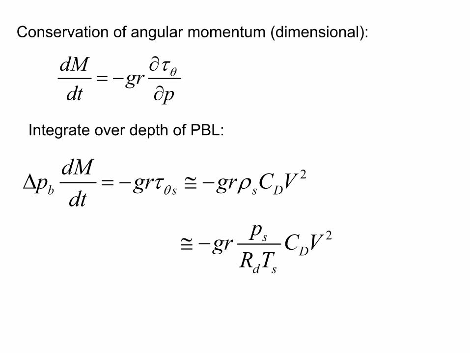
Conservation of angular momentum (dimensional):

dM grdt p

θτ∂= −∂

Integrate over depth of PBL:

2

2

b s s D

sD

d s

dMp gr gr C Vdt

pgr C VR T

θτ ρ∆ = − ≅ −

≅ −

Scaling for time:

11 2d sD b s

s

R Tt C p tgp

χ −−→ ∆

Nondimensional angular momentum equation:2

But

12

2

dR Vrdt R

Rr2V

dR RVdt

= −

→ − (2)

Nondimensional PBL entropy equation:

( )* 30 ,k

bD

s o

s

Cd V V Fdt C

T TT

χ χ χ ε

ε

= − + −

−≡

Time derivative in R space:

d Rdt R P

ωτ∂ ∂ ∂

= + +∂ ∂ ∂

(3)

Assume Χ well mixed in boundary layer,

use 1 :2

R RV= −

Also assume that Fb balances source terms outside of eyewall:

( )* 30

12

0

k

D

CRV V V eyewallR C

elsewhere

χ χ χ ε

χτ

∂+ − +

∂∂

=∂

2 *2 2R RBut V in eyewall

R Rχ χ∂ ∂

− = −∂ ∂

( ) ( )* 30 1 ,

10

k

D

C V VC

in eyewallelsewhere

χ β χ χ ετ

ββ

∂→ = − − − ∂ ==

(Steady state solution:)

( )2 *0

11

k

D

CVC

χ χε

= −−

(4)

Differentiate (4) with respect to R and use 2 :2RVRχ∂

−∂

( ) ( )

( ) ( )

2 *0

2

2 *0

3 14

2

14

k

D

k

D

k

D

CV R V VV R CC VC

CR VR C

β ε χ χτ

β

β ε χ χ

∂ ∂= − − − ∂ ∂

−

∂+ − − − ∂

First term: Propagation; Second term: damping;

Third term: Amplification

Note that first term steepens V gradient when 2 2maxV V>

0 necessary for amplificationRβ∂<

∂V gradient cannot steepen indefinitely:

( )

( )

,

1 1

1

1

V Vr rR r V V r

r r R R r r R R RV r Vr R R

V r Vr R Rr VR R

ς

ς

ς ς

ς

∂= +

∂∂ ∂ ∂ ∂ ∂ ∂ = = + + = + ∂ ∂ ∂ ∂ ∂ ∂

∂→ = + +

∂∂

+∂=∂

−∂

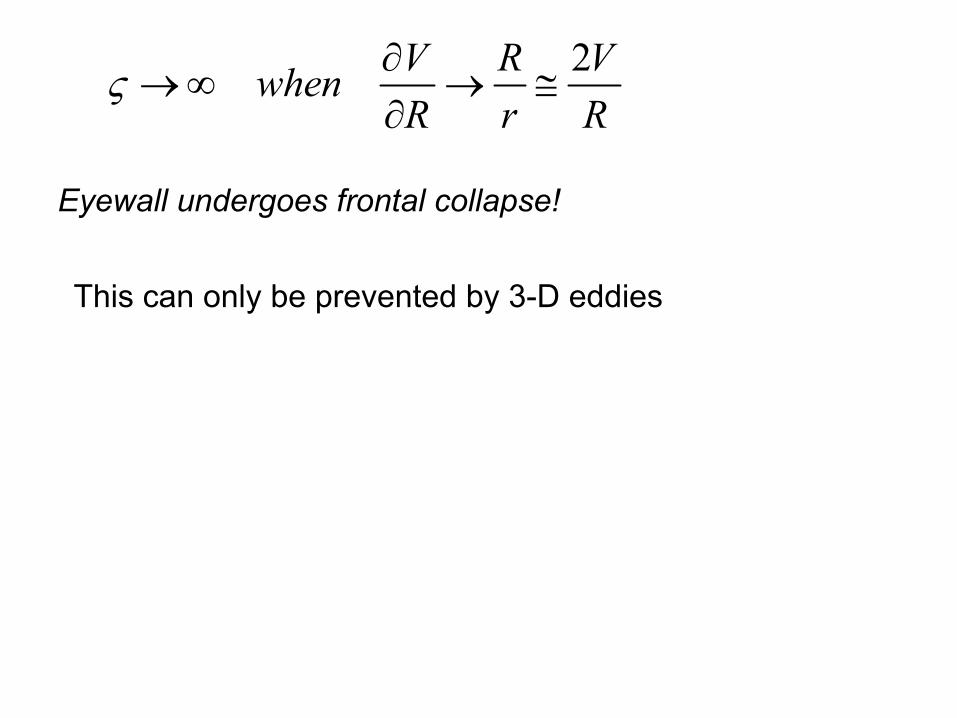
2V R VwhenR r R

ς ∂→∞ → ≅

∂

Eyewall undergoes frontal collapse!

This can only be prevented by 3-D eddies

12

R RV−

Simplified amplification model:

( ) ( )* 30 1 ,

10

k

D

C V VCin eyewallelsewhere

χ β χ χ ετ

ββ

∂= − − − ∂

==

* 20

11 12

AP A Vχ χ = − = + +

2 *2RV

Rχ∂

= −∂

*Enforce χ χ≤

How to handle frontal collapse in model?

Three methods:

1: Zero diffusion model:

For r < rm:0*

Vconstantχ χ

== =

Does not prevent frontal collapse

2. Minimum diffusion model: Just enough radial diffusion to prevent failure of coordinate transformation.

From expression for vertical component of vorticity, we enforce

2V VR R∂

≤∂

Inside the outermost radius, Rcrit, where this is violated, we take

2

2

critcrit

V VR R

RV VR

∂=

∂

→ =

By integration of2* 2V

R Rχ∂

= −∂

421* 1 ,

2

*

crit crit critcrit

crit

RV for R RR

for R R

χ χ

χ χ

= + − <

= ≥

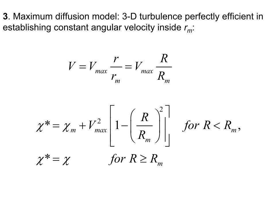
3. Maximum diffusion model: 3-D turbulence perfectly efficient in establishing constant angular velocity inside rm:

max maxm m

r RV V Vr R

= =

22* 1 ,

*

m max mm

m

RV for R RR

for R R

χ χ

χ χ

= + − <

= ≥

Tropical Cyclone Structure

• Hydrostatic and gradient balance above PBL everywhere

• Moist adiabatic lapse rates on angular momentum surfaces above PBL everywhere

• Boundary layer quasi-equilibrium (with horizontal entropy advection and dissipative heating) in rain area

• Radiative-subsidence balance in outer region

Boundary layer quasi-equilibrium

Assume that boundary layer entropy changes slowly in angular momentum space:

ds s dM sdt dt Mτ

∂ ∂= +∂ ∂

( ) ( )( )* 3| | | | .s k s D u b m ss dM shT C k k C M w h h hT

dt Mτ∂ ∂

= − + − − − −∂ ∂

V V

PBL angular momentum: | |DdMh C r Vdt

= − V

( ) ( )( )* 3| | | | | | .s k s D u b m s Ds shT C k k C M w h h T C r V

Mτ∂ ∂

= − + − − − +∂ ∂

V V V

(1)

In rain area, 0, *:uM s s> =

Use thermal wind balance, neglecting

| | | | .ss D D

s o

Ts MT C r V C VM T T r∂

−∂ −

V V

2

1 :or

Use in (1), approximating | | :M by V and by Vr

V

( )* 31 .ou k s D

b m s o

TM w C V k k C Vh h T T

= + − − − −

(2)

Closure for convective updraft mass flux.

Free tropopshere thermodynamic balance:

( )* d d radu d

m

s Qs M M wz Tτ

Γ ∂∂= − − + ∂ Γ ∂

Representation of downdrafts:

(1 ) ,d uM Mε= −

(3)

Steady state version of (3):

,rad uw w Mε= − +

radrad

d

Qw sTz

≡ − ∂∂

(4)

Outside rain area,

01

rad uw w Mr r

ψ=

∂= = −

∂

Within rain area, substitute (2) into (4):

( ) ( )* 311 0.orad k s D u

b m s o

Tw C V k k C V Mr r h h T T

ψ εε ∂

− = − + − − > ∂ − −

System closed using PBL angular momentum balance:

2 2 ,DM C r Vr

ψ ∂=

∂

or, equivalently,

(5)

(6)

( ) 2 2

.DrV C r V frr ψ

∂= −

∂

Apply scaling:

max ,V v V→

max ,vr rf

→

3max2 ,D

vCf

ψ ψ→

max ,rad D Qw C v w→

max ,u D uM C v M→

Nondimensional system:

( ) 2 2

,rV r V rr ψ

∂= −

∂

1 0,Q uw for Mr r

ψ∂= − =

∂

( )31 0,Q uw V V for Mr rε ψ ε− ∂

= − + Λ − >∂

( )311u QM w V V

ε = − +Λ − −

*k s

D b m

C k kC h h

−Λ ≡

−

(7)

(8)

(9)

(10)

Boundary condition: 00 at r rψ = =

From (7): 00V at r r= =

Simple case: , , constantQwεΛ

Outside rain area, solution to (8) is then

( )2 212 Q ow r rψ = −

Substitute into (7):

( )( )2 2

2 2

2

Q o

rV r V rr w r r

∂= −

∂ −

For wQ << 1, dominant balance is

2 22 12

oQr rV wr−

≈

For 2 20 ,r r<<

12V r

−≈

In rain area, assume that QV wεΛ >> 2 1V <<

,1

rVrψ ε

ε∂ Λ∂ −

( )2 2

.r VrVr ψ∂∂

(11)

(12)

(11) and (12) have power law solution:

nV r−≈

( )( )2 1

.1

nε εε εΛ − −

≡Λ − −

Realistic only if

12 .εε−

Λ >

(In numerical solutions to be presented, 23n = )

Numerical solution of (7)-(10): March inward from 0 :r r=

Note: longer tail in R&E model owing to different formulation of Q

1Λ =

0.8ε =

0.1Qw =

0.25or =

Curve fit to numerical solutions:

( )( )( )

( )2 22 2 0

2 120

1 1 2,

1 2

m

m mn mm m

mm

b n m b mr r rV Vr r r rr mn m

rr

++

− + + − = + − ++