Tropical Cyclone Research Report No. 2 TROPICAL …roger/Publications/M6on.pdfTropical-cyclone ﬂow asymmetries induced by a uniform ﬂow revisited Gerald L. Thomsen a, Roger K

Tropical Cyclone Research Report No. 2

TROPICAL-CYCLONE FLOW ASYMMETRIES INDUCED BY A

UNIFORM FLOW REVISITED

Gerald L. Thomsen, Roger K. Smith

Meteorological Institute, Ludwig Maximilians University of

Munich, Munich, Germany.

and

Michael T. Montgomery

Dept. of Meteorology, Naval Postgraduate School, Monterey,

CA, USA

April 2012

Meteorological Institute

Ludwig Maximilians University of Munich

Theresienstrasse 37

80333 Munich, Germany

http://www.meteo.physik.uni-muenchen.de

Tropical-cyclone flow asymmetries induced by a uniform flowrevisited

Gerald L. Thomsen a, Roger K. Smith a ∗and Michael T. Montgomery b

a Meteorological Institute, University of Munich, Munich, Germany,b Dept. of Meteorology, Naval Postgraduate School, Monterey, CA & NOAA’s Hurricane Research Division

∗Correspondence to: Roger K. Smith, Meteorological Institute, University of Munich, Theresienstr. 37, 80333 Munich,Germany. Email: [email protected]

Idealized three-dimensional numerical model simulations are carried out toinvestigate the hypothesized effects of a uniform flow on the intensification,structural evolution, and maximum intensity of a tropical cyclone. At any onetime, the presence of explicit deep convection in the model tends to mask theflow asymmetries predicted by earlier theoretical studies. In sets of ensembleexperiments in which the initial low-level moisture field is randomly perturbed,a coherent asymmetry in vertical velocity for strong vortices (maximum windspeeds ≈ 80 m s−1) is found only for background wind speeds larger thanabout 7 m s−1. In these experiments, time-averaged ensemble mean fields inthe mature stage show an asymmetry in the vertical motion rising into theeyewall. However, the maximum ascent occurs about 45 degrees to the leftof the vortex motion vector, consistent with one earlier calculation by Frankand Ritchie, but different from the predictions of previous studies that do notexplicitly account for deep convection. The corresponding mean storm-relativemaximum tangential wind speed occurs on the left side of the motion vector as inrecent observations of boundary-layer flow asymmetries in translating storms.However, there is considerable variability in the structure of the low-level flowon a sub-hourly time scale as a result of transient convection, a finding thatraises questions concerning the ability to be able to reliably determine vortex-scale flow asymmetries (especially in the radial direction) from dropwindsondeobservations spread over several hours.Copyright c© 2012 Royal Meteorological Society

Key Words: Hurricane; tropical cyclone; typhoon; boundary layer; vortex intensification

Received 27 May 2011; Revised April 26, 2012; Accepted

Citation: . . .

1. Introduction

In a recent paper, Nguyen et al. (2008, henceforth M1)investigated the predictability of tropical-cyclone inten-sification in a three-dimensional numerical model. Theyfocussed on two prototype problems for intensification,which consider the evolution of a prescribed, initially cloud-free, axisymmetric, baroclinic vortex over a warm ocean onan f -plane or beta-plane. A companion study of the sameproblems using a minimal three-dimensional model wascarried out by Shin and Smith (2008). Both studies found

that on an f -plane, the flow asymmetries that develop arehighly sensitive to the initial low-level moisture distribution.When a random moisture perturbation is added in theboundary layer at the initial time, even with a magnitudethat is below the accuracy with which moisture is normallymeasured, the pattern of evolution of the flow asymmetriesis dramatically altered and no two such calculations arealike in detail. The same is true also of calculations ona β-plane, at least in the inner-core region of the vortex,within 100-200 km from the centre. Nevertheless the large-scale β-gyre asymmetries are similar in each realization

Copyright c© 2012 Royal Meteorological Society

Prepared using qjrms4.cls [Version: 2011/05/18 v1.02]

and they remain when one calculates the ensemble mean.The implication is that the inner-core asymmetries on thef - and β-plane result from the onset of deep convectionin the model and, like deep convection in the atmosphere,they have a degree of randomness, being highly sensitiveto small-scale inhomogeneities in the low-level moisturedistribution. Such homogeneities are a well-known charac-teristic of the real atmosphere (e.g. Weckwerth, 2000).

In the foregoing flow configurations, there was noambient flow and an important question remains: could theimposition of a uniform flow or a vertical shear flow leadto an organization of the inner-core convection, therebymaking its distribution more predictable? For example,there is evidence from observations (Kepert 2006a,b,Schwendike and Kepert 2008) and from steady boundarylayer models with varying degrees of sophistication that atranslating vortex produces a distinct asymmetric patternof low-level convergence and vertical motion (Shapiro,1983, Frank and Richie 1999, Kepert 2001, Kepert andWang 2001). There is much evidence also that verticalshear induces an asymmetry in vortex structure (Raymond1992, Jones 1995, 2000a,b, Smith et al. 2000, Frank andRitchie 1999, 2001, Reasor and Montgomery 2001, 2004,Corbosiero and Molinari 2002, 2003, Riemer et al. 2010).

The important observational study by Corbosiero andMolinari (2003) showed that the distribution of strongconvection is more strongly correlated with vertical shearthan with the storm translation vector. Nevertheless, thequestion remains as to whether storm translation isimportant in organizing convection in the weak shear case.Although the main purpose of Frank and Richie (2001) wasto investigate the effects of vertical shear in a moist model,they did carry out one simulation for a uniform flow. Inthis they found that ” ... the upward vertical motion patternvaries between periods that are almost axisymmetric andother periods when they show more of a wavenumber oneasymmetry, with maximum upward motion either ahead orto the left of the track.” and ”the frictional convergencepattern in the boundary layer causes a preference forconvective cells to occur generally ahead of the stormrelative to behind it, but this forcing is not strong enoughto maintain a constant asymmetric pattern.” This finding iscontrary to the predictions of a steady boundary layer forcedby an imposed gradient wind field above the layer as in theother uniform flow studies cited above.

As noted in M1 and Shin and Smith (2008), therandom nature of the inner-core asymmetries calls fora new methodology to assess differences between twoparticular flow configurations, because the results of a singledeterministic calculation in each configuration may beunrepresentative of a model ensemble in that configuration.Thus one needs to compare the ensemble means of suitablyperturbed ensembles of the two configurations. We applythis methodology here to extend the calculations of M1to the prototype problem for a moving vortex, whichconsiders the evolution of an initially dry, axisymmetricvortex embedded in a uniform zonal flow on an f -plane.

Even in the relatively simple case of a uniform flow, thereis some disagreement in the literature on the orientation offlow asymmetries that arise. For example, using a nonlinear,slab boundary layer model with constant depth, Shapiro(1983) shows that the strongest convergence (and hencevertical velocity in his model) occurs on the forward side ofthe vortex in the direction of motion (see his Figures 5d and

6c). In contrast, the purely linear theory of Kepert (2001, leftpanel of Figure 5) predicts that the strongest convergencelies at 45 degrees to the right of the motion and the nonlinearcalculations of Kepert and Wang (2001, bottom left panelof Figure 10) predicts it to be at 90 degrees to the rightof motion. As noted by the respective authors, a limitationof the foregoing studies is the fact that the horizontal flowabove the boundary layer is prescribed and not determinedas part of a full solution.

Here we seek to answer the four questions:

1 Does the imposition of a uniform flow significantlyaffect the intensification rate and mature intensity fortypical storm translation speeds in the tropics?

2 Does the imposition of a uniform flow in aconvection-permitting simulation lead to an organiza-tion of the inner-core convection to produce persistentasymmetries in convergence and vertical motion?

3 If so, are these asymmetries similar to those predictedby earlier studies where the horizontal flow above theboundary layer is prescribed?

4 How do the asymmetries in low-level flow structureassociated with the storm translation compare withthose documented in recent observational studies?

We are aware of three previous modelling studiesaddressing the first question above (Peng et al. 1999,Dengler and Keyser 2000, Wu and Braun 2004). All threestudies found a systematic reduction of intensity withtranslation speed. Peng et al. attributed this reduction to anout of phase relationship between the asymmetry in surfacemoisture flux and boundary-layer moisture convergence. Incontrast, Dengler and Keyser found that, in their three-layer model, it was the penetration of stable dry air frommid-levels to the boundary layer that reduced the stormintensity. Finally, Wu and Braun (2004) suggested thatthe inhibiting effect of an environmental flow is closelyassociated with the resulting eddy momentum flux, whichtends to decelerate tangential and radial winds in bothinflow and outflow layers. The corresponding changes in thesymmetric circulation tend to counteract the decelerationeffect. The net effect is a moderate weakening of themean tangential and radial winds. Interestingly, the firsttwo of these studies give thermodynamic arguments for thevortex behaviour in a mean flow while the third gives aninterpretation based on dynamical processes.

All the foregoing studies used models employing arelatively coarse horizontal resolution by today’s standards(Peng et al. used 0.5o latitude, Dengler and Keyser 20 km,and Wu and Braun 25 km) and relied on a parameterizationof deep cumulus convection. Both Peng et al. and Wuand Braun used the Kuo scheme, which has been heavilycriticized because of its use of moisture convergence asthe basis for its closure∗. Dengler and Keyser used thesimple scheme proposed by Ooyama (1969) in which thecloud-base mass flux is equal to the resolved-scale massflux in the boundary layer. Because of the uncertaintiesunderlying the parameterization of deep convection in thesestudies, and because of recent insights into the role of deepconvection on tropical-cyclone intensification that haveemerged in the last few years, it seems appropriate to revisitquestion [1] above. In fact, Wu and Braun recommendfurther investigation of the various physical mechanisms

∗See Raymond and Emanuel (1993).

Copyright c© 2012 Royal Meteorological Society Q. J. R. Meteorol. Soc. 00: 1–17 (2012)

Prepared using qjrms4.cls

responsible for tropical-cyclone intensity (resulting fromlarge-scale influences) using high-resolution simulationswith more sophisticated model physics.

The remainder of the paper is structured as follows. Wegive a brief description of the model in section 2 and presentthe results of the main calculations for vortex evolutionon an f -plane in section 3. In section 4 we describe theensemble experiments, where, as in M1, the ensembles aregenerated by adding small moisture perturbations at lowlevels. We examine the asymmetric structure of boundarylayer winds in section 5 and describe briefly a calculationusing a different boundary-layer scheme section 6. Theconclusions are given in section 7.

2. The model configuration

The numerical experiments are similar to those describedin M1 and are carried out also using a modified versionof the Pennsylvania State University-National Center forAtmospheric Research fifth-generation Mesoscale Model(MM5; version 3.6, Dudhia 1993; Grell et al. 1995).The model is configured with three domains with sidesorientated east-west and north-south (Figure 1). The outerand innermost domains are square, the former 9000 km insize and the latter 1500 km. The innermost domain is movedfrom east to west at selected times within an intermediatedomain with a fixed meridional dimension of 3435 kmand a zonal dimension of up to 8850 km, depending onthe background wind speed. The first displacement takesplace 735 minutes after the initial time and at multiplesof 1440 minutes (one day) thereafter. The frequency ofthe displacement is doubled for a background wind speedof 12.5 m s−1. The distance displaced depends on thebackground wind speed in the individual experiments. Theouter domain has a relatively coarse, 45-km, horizontal gridspacing, reducing to 15 km in the intermediate domain and5 km in the innermost domain. The two inner domains aretwo-way nested. In all calculations there are 24 σ-levels inthe vertical, 7 of which are below 850 mb. The model top isat a pressure level of 50 mb. The calculations are performedon an f -plane centred at 20◦N.

To keep the experiments as simple as possible, wechoose the simplest explicit moisture scheme, one thatmimics pseudo-adiabatic ascent†. In addition, for allbut one experiment we choose the bulk-aerodynamicparameterization scheme for the boundary layer. Oneadditional calculation is carried out using the Gayno-Seaman boundary-layer scheme (Shafran et al. 2000) toinvestigate the sensitivity of the results to the scheme used.

The surface drag and heat and moisture exchangecoefficients are modified to incorporate the results ofthe coupled boundary layer air-sea transfer experiment(CBLAST; see Black et al. 2007, and Zhang et al. 2009).The surface exchange coefficients for sensible heat and

†If the specific humidity, q, of a grid box is predicted to exceed thesaturation specific humidity, qs(p, T ) at the predicted temperature T andpressure p, an amount of latent heat L(q − qs) is converted to sensible heatraising the temperature by dT = L(q − qs)/cp and q is set equal to qs,so that an amount of condensate dq = q − qs is produced. (Here L is thecoefficient of latent heat per unit mass and cp is the specific heat of dry airat constant pressure.) The increase in air parcel temperature increases qs,so that a little less latent heat than the first estimate needs to be released anda little less water has to be condensed. The precise amount of condensationcan be obtained by a simple iterative procedure. Convergence is so rapidthat typically no more than four iterations are required.

(a)

Figure 1. Configuration of the three model domains. The inner domain ismoved from east to west (the negative x-direction) at selected times to keepthe vortex core away from the domain boundary.

moisture are set to the same constant, 1.2× 10−3, and thatfor momentum, the drag coefficient, is set to 0.7× 10−3 +1.4× 10−3(1− exp(−0.055|u|)), where |u| is the windspeed at the lowest model level. The fluxes between theindividual model layers within the boundary layer are thencalculated by a first-order (local K-mixing) scheme.

The exchange coefficient for moisture is set to zero inthe two outer domains to suppress the build up there ofambient Convective Available Potential Energy (CAPE).Because of the dependence of the moisture flux on windspeed, such a build up would be different in the experimentswith different wind speeds. The sea surface temperature isset to a constant 27oC except in one experiment where it wasset to 25oC to give a weaker mature vortex. The radiativecooling is implemented by a Newtonian cooling term thatrelaxes the temperature towards that of the initial profileon a time scale of 1 day. This initial profile is defined inpressure coordinates rather than the model’s σ-coordinatesso as not to induce a thermal circulation between southernand northern side of the model domain.

In each experiment, the initial vortex is axisymmetricwith a maximum tangential wind speed of 15 m s−1 at thesurface at a radius of 120 km. The strength of the tangentialwind decreases sinusoidally with height, vanishing at thetop model level (50 mb). The vortex is initialized to be inthermal wind balance with the wind field using the methoddescribed by Smith (2006). The far-field temperature andhumidity are based on Jordan’s Caribbean sounding (Jordan1958). The vortex centre is defined as the centroid of relativevorticity at 900 mb over a circular region of 200 km radiusfrom a “first-guess” centre, which is determined by theminimum of the total wind speed at 900 mb.

2.1. The main experiments

Six main experiments are discussed, five with a uniformbackground easterly wind field, U , and the other withzero background wind. Values of U are 2.5 m s−1, 5 ms−1, 7.5 m s−1, 10 m s−1 and 12.5 m s−1, adequatelyspanning the most common range of observed tropical-cyclone translation speeds. All these experiments employ



Figure 2. Time series of maximum total wind speed at 850 mb, V Tmax,for the six experiments with different background wind speeds U : (black:U = 0 m s−1, red: U = 2.5 m s−1, blue: U = 5.0 m s−1, purple:U = 7.5 m s−1, orange: U = 10 m s−1, pink: U = 12.5 m s−1) and forthe experiment with U = 5.0 m s−1 but with the sea surface temperaturereduced to 25oC. The time series have been smoothed with a five-pointfilter to highlight the differences between them.

the bulk aerodynamic representation of the boundary layerand have a sea surface temperature (SST) of 27oC. Twoadditional experiments have U = 5 m s−1, one with an SSTof 25oC, and the other with the Gayno-Seaman boundary-layer scheme.

2.2. Ensemble experiments

As in M1, sets of ensemble calculations are carriedout for the main experiments. These are similar to themain calculations, but have a random perturbation witha magnitude between ±0.5 g kg−1 added to the water-vapour mixing ratio at each grid point up to 950 mb atthe initial time. In order to keep the mass field unchanged,the temperature is adjusted at each point to keep thevirtual temperature unchanged. A five member ensemble isconstructed for all values of U except U = 5 m s−1, forwhich a ten member ensemble is constructed.

3. Results of five deterministic calculations

3.1. Vortex evolution and motion

Figure 2 shows time-series of the maximum total windspeed, V Tmax at 850 mb (approximately 1.5 km high)during a 7 day (168 hour) integration in the six mainexperiments and in that with U = 5 m s−1 and an SSTof 25oC. The last experiment will be discussed in section3.3. As in many previous experiments, including those inM1, the evolution begins with a gestation period duringwhich the vortex slowly decays due to surface friction, butmoistens in the boundary layer due to evaporation from theunderlying sea surface. This period lasts approximately 9hours during which time the maximum total wind speeddecreases by about 2.0 m s−1.

The imposition of friction from the initial instantleads to inflow in the boundary layer and outflowabove it, the outflow accounting for the initial decrease

in tangential wind speed through the conservation ofabsolute angular momentum. The inflow is moist and asit rises out of the boundary layer and cools, condensationprogressively occurs in some grid columns interior to thecorresponding radius of maximum tangential wind speed.In these columns, existing relative vorticity is stretchedand amplified leading to the formation of localized deepvortical updraughts. Collectively, these updraughts lead tothe convergence of absolute angular momentum above theboundary layer and thereby to the spin up of the bulkvortex (see e.g. Bui et al. 2009). Then, as the bulk vortexintensifies, the most intense tangential wind speeds developin the boundary layer (Smith et al. 2009).

As the updraughts develop, there ensues a periodlasting about 5 days during which the vortex progressivelyintensifies. During this time, V Tmax increases from itsminimum value of between 12.5 and 25 m s−1 to a finalvalue of up to 90 m s−1 at the end of the experiment.The vortex in the quiescent environment is the first toattain a quasi-steady state after about 6 days, but allexcept possibly that for U = 10 m s−1 appear to havereached such a state after 7 days. For all values of U ,there are large fluctuations in V Tmax (up to ±5 m s−1

before time-smoothing) during the period of intensification.Indeed, except in the experiment with an SST of 25 oC, thefluctuations in an individual experiment during this periodare comparable with the maximum deviations between thedifferent experiments to the extent that it is pertinent to askif the differences between these experiments are significant.We examine this important question in section 4.1.

The translation speed tends to be fractionally smallerthan the background wind speed, especially in the maturestage when it is between 20% and 25% less. The translationspeeds for U = 7.5 m/s, 10 m/s and 12.5 m/s are about 5.9,7.5 and 9.5 m/s, respectively. This is presumably becausethe tangential circulation of the vortex is strongest at lowlevels where the background wind is, itself, reduced instrength by surface friction.

3.2. Structure changes

The evolution in vortex structure during the intensificationstage is exemplified by the contours of vertical velocity at850 mb at selected times for the main experiment with U =5 m s−1. These contours are shown in Figures 3 and 4. Atearly times, convective cells begin to develop in the forwardleft (i.e. southwest) quadrant (Figure 3a), where, as shownbelow, the boundary-layer-induced convergence is large.However, cells subsequently develop clockwise (upstream)in the space of two hours to the forward quadrant (Figure3b) and over the next two hours to the forward right and rearright quadrants (Figure 3c). It should be emphasized that, asin the calculations in M1, the cells are deep, extending intothe upper troposphere (not shown here).

By 24 hours, convective cells are distributed over allfour quadrants with little obvious preference for a particularsector. Moreover, they amplify the vertical component oflocal low-level relative vorticity by one or two orders ofmagnitude (not shown). For comparison, panels (e) and (f)of Figure 3 show the early evolution of cells in the maincalculation with zero background flow, which, as expected,shows no preference for cells to develop in a particularsector.

As time proceeds, the convection becomes moreorganized (Figure 4), showing distinctive banded structures,



(a) (b)

(c) (d)

(e) (f)

Figure 3. Contours of vertical velocity at 850 mb at times indicated in the top right of each panel during the vortex evolution. (a)-(d) for the experimentwith U = 5.0 m s−1 (from right to left), and (e) and (f) for the experiment with the zero background flow. Contour interval: thick contours 0.5 m s−1,thin contours 0.1 m s−1. Positive velocities (solid/red lines), negative velocities (dashed/blue lines). The zero contour is not plotted. The arrow indicatesthe direction of vortex motion.

but even at 90 h, its distribution is far from axisymmetric,even in the region within 100 km of the axis. However,

as shown later, the vortex does develop an annular ring of



(a) (b)

Figure 4. Contours of vertical velocity at 850 mb at (a) 60 hours, and (b) 96 hours, during the vortex evolution for the experiment with U = 5.0 ms−1 (from right to left). Contour interval: thick contours 0.5 m s−1, thin contours 0.1 m s−1. Positive velocities (solid/red lines), negative velocities(dashed/blue lines). The zero contour is not plotted. The arrow indicates the direction of vortex motion.

(a) (b)

Figure 5. Contours of divergence at 500 m at for the experiment with U = 5.0 m s−1: (a) between 3-5 hours (contour interval 1× 10−5 s−1. Positivecontours (solid/red) and negative values (dashed/blue).) and (b) between 63

4− 7 days (contour interval: thick contours 5× 10−4 s−1, thin contours

5× 10−5 s−1. Positive contours (solid/red), negative values (dashed/blue)), zero contour thin, solid and black. The arrow indicates the direction ofvortex motion. Note that the domain shown is only half the size of that in Figures3 and 4.

convection with an eye-like feature towards the end of theintegration.

Figure 5 shows the pattern of convergence at a heightof 500 m averaged between 3 and 5 h and 6 3

4 − 7 days inthe case with U = 5 m s−1. This height is typically thatof the maximum tangential wind speed and about half thatof the ‘mean’ inflow layer in the mature stage (see section5). The period 3-5 hours is characteristic of the gestationperiod during which the boundary layer is moistening, butbefore convection has commenced. During this period, theconvergence is largest on the forward side of the vortex,explaining why the convective instability is first releasedon this side. There is a region of divergence in the rear leftsector. The pattern is similar to that predicted by Shapiro

(1983‡), but in Shapiro’s calculation, which, at this stagewas for a stronger symmetric vortex with a maximumtangential wind speed of 40 m s−1 translating at a speedof 10 m s−1, the divergence region extends also to the rearright of the track.

In the mature stage in our calculation, the pattern ofconvergence is rather different from that in Shapiro’scalculation and is much more symmetric, presumablybecause at this stage the vortex is twice as strong asShapiro’s and the translation speed is only half. Notably,outside the ring of strong convergence that marks the

‡See his Figure 5d, but note that the vortex translation direction is orienteddifferently to that in our configuration.



(a) (b)

Figure 6. Contours of divergence at 500 m at for the experiment with U = 5.0 m s−1 and a sea surface temperature of 25oC: (a) between 3-5 hours(contour interval 1× 10−5 s−1). (b) between 63

4− 7 days (contour interval: thick contours 5× 10−4 s−1, thin contours 5× 10−5 s−1. Positive

contours (solid/red), negative values (dashed/blue), zero contour thin, solid and black. The arrow indicates the direction of vortex motion. Note that thedomain shown is only half the size of that in Figure4.

eyewall, the vortex is almost surrounded by a region of low-level divergence, except for the narrow band of convergencefeeding into the eyewall on the forward right side. In thenext section we examine the differences in behaviour for aweaker vortex.

3.3. Calculations for a weaker vortex

To examine the questions raised in the previous sectionconcerning possible differences when the vortex is muchweaker, we repeated the experiment with U = 5 m s−1 withthe sea surface temperature reduced by 2oC to 25oC. Figure2 shows the variation of total wind speed at 850 mb in thiscase. As expected, the evolution is similar to that in Figure3, but the maximum wind speed during the mature stage isconsiderably reduced, with the average wind speed duringthe last 6 hours of the calculation being only about 40 ms−1. Figure 6 shows the patterns of divergence at a heightof 500 m averaged during 3-5 hours and during the last 6hours of this calculation. These should be compared withthe corresponding fields in Figure 5. In the early period(panel (a)), the patterns are much the same, although themaximum magnitudes of divergence and convergence areslightly larger when the sea surface temperature is reduced.We have no explanation for this difference, but do notconsider it to be significant. In the mature stage (panel(b)), the differences are considerable with the central ringof divergence marking the eye being much larger in thecase of the weaker vortex and the region of convergencesurrounding it and marking the eyewall being broader andmore asymmetric. However, like the stronger vortex and thatin Shapiro’s calculation, the largest convergence is on theforward side of the vortex with respect to its motion.

4. Ensemble experiments

As pointed out by M1 and Shin and Smith (2008), theprominence of deep convection during the vortex evolutionand the stochastic nature of convection, itself, means that

the vortex asymmetries will have a stochastic componentalso. Thus, a particular asymmetric feature brought aboutby an asymmetry in the broadscale flow (in our casethe uniform flow coupled with surface friction) may beregarded as significant only if it survives in an ensembleof experiments in which the details of the convectionare different. For this reason, we carried out a seriesof ensemble experiments in which a random moistureperturbation is added to the initial condition in the mainexperiments as described in section 2.2. We begin byinvestigating the effects of this stochastic component on thevortex intensification and go on to examine the effects onthe vortex structure in the presence of uniform flows withdifferent magnitudes.

4.1. Stochastic nature of vortex evolution

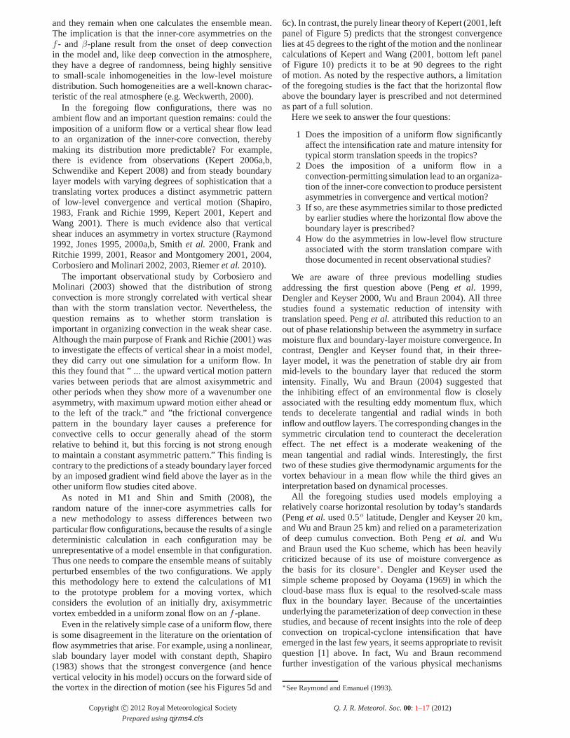
Figure 7a shows time series of the ensemble-mean,maximum total wind speed, V Tmax, at 850 mb for the mainexperiments with background flows of 5 m s−1 and 10 ms−1. It shows also the range of variability (i.e. the maximumand minimum values of V Tmax) for the set of ensembles ineach case. There are two features of special interest:

• There is a significant difference between themaximum and minimum intensity at any one time,being as high as 20 m s−1 in the case U = 10 m s−1

at about 6 days.• There is some overlap between the envelopes of

variability between the two sets of ensembles, butafter about 5 days, the ensemble mean V Tmax of theset with U = 10 m s−1 is generally smaller than thatof the set with U = 5 m s−1.

The foregoing comparison suggests that the differencesin intensity between the main experiments with differentvalues of background flow shown in Figure 2 may not besignificant and that one should really examine ensemblemean values rather than time series of single deterministic



(a) (b)

Figure 7. (a) Time series of the ensemble-mean, maximum total wind speed, V Tmax, at 850 mb for the main experiments with a background flow of 5m s−1 (middle red curve) and 10 m s−1 (middle blue curves). The thin curves of the same colour show the maximum and minimum values of V Tmax

for a particular run at a given time. (b) Time series of the ensemble-mean V Tmax for the experiments with U = 0, 5, 7.5, 10 and 12.5 m s−1.

runs. Such a comparison is made in Figure 7b, whichshows time series of the ensemble mean for the experimentswith U = 0, 5, 7.5, 10 and 12.5 m s−1. It is clearfrom this figure that the intensification rate decreases withincreasing background flow speed and that the maturevortex intensity decreases also, although the differencesbetween the intensity of the pairs of ensembles withU = 5 and 7.5 m s−1 and U = 10 and 12.5 m s−1

after 7 days is barely significant. Finally we note thatcomparison of plots of the eleven§ V Tmax-time series forU = 5 m s−1 with the six such time series for the otherensemble sets suggests that five ensembles together with thecorresponding control experiment give an acceptable spanof the range of variability in each case (not shown).

When viewed in the proper way, the foregoing results areconsistent with those of Zeng et al. (2007), who presentedobservational analyses of the environmental influences onstorm intensity and intensification rate based on reanalysisand best track data of Northwest Pacific storms. While theyconsidered a broader range of latitudes, up to 50 oN, and ofstorm translation speeds of up to 30 m s−1, the data thatare most relevant to this study pertain to translation speedsbetween 3 and 12 m s−1. The most intense tropical cyclonesand those with the most rapid intensification rates werefound to occur in this range when there is relatively weakvertical shear. Most significantly, their data have a lot ofscatter in this range and do not show an obvious relationshipbetween intensity and translation speed.

4.2. Stochastic nature of vortex structure

The first four panels of Figure 8 show the time-averaged vertical velocity fields for the last 6 hours ofintegration (6 3

4 - 7 days) in three of the experimentswith U = 10.0 m s−1, including the main experimentand two ensemble experiments and in the six-memberensemble mean. In all fields, including the ensemble mean,there is a prominent azimuthal wavenumber-1 asymmetry,with maximum upflow in the forward left quadrant andmaximum subsidence in the eye to the left of the motion

§We include the main calculation as part of the ensemble mean whenaveraging.

vector. Similar results are obtained for U = 7.5 m s−1

and 12.5 m s−1 (not shown). For U = 5 m s−1, the mostprominent asymmetry in the vertical velocity is at azimuthalwavenumber-4 (Fig. 8f), which is a feature also of theensemble mean of calculations for a quiescent environment(Fig. 8e). As the latter would be expected to have noasymmetry for a sufficiently large ensemble, we are inclinedto conclude that the wavenumber-4 asymmetry in the casewith U = 5 m s−1 is at least partially a feature of thelow ensemble sample and possibly also of the limited gridresolution (the 100 km square domain in Figure 8 is spannedby only 21× 21 grid points). Therefore we do not attributemuch significance to the wavenumber-4 component of theasymmetry in panels (e)-(f).

On the basis of these results, we are now in a positionto answer the second of the four questions posed in theIntroduction: does the imposition of a uniform flow in aconvection-permitting simulation lead to an organization ofthe inner-core convection so as to produce asymmetries inlow-level convergence and vertical motion? The answer tothis question is a qualified yes, the qualification being thatthe effect is barely detectable for the strong vortices thatarise in our calculations and for background flow speedsbelow about 7 m s−1. However, the effect increases withbackground flow speed and there is a more prominentazimuthal wavenumber-1 asymmetry in the calculation for aweaker storm with U = 5 m s−1 (see section 3.3 and Figure6b).

We are in a position also to answer the third of the fourquestions: how do the asymmetries compare with thosepredicted by earlier studies? For background flow speeds of7.5 m s−1 and above, the ensemble mean vertical velocityasymmetry, which for upflow is in the forward left quadrantin our calculations, is closest to the prediction of Shapiro(1983). Whereas, Shapiro found the maximum convergence(and hence vertical motion in his slab model) to be directlyahead of the motion vector, we find it to be approximately45o to the left thereof. Our result deviates significantly fromthat in Kepert’s (2001) linear theory, where the maximumvertical motion is at 45o to the right of the motion vector andeven more from that in the nonlinear numerical calculationof Kepert and Wang (2001), where the maximum is at 90 o

to the right of the motion vector. The reasons for these



(a) (b)

(c) (d)

(e) (f)

Figure 8. Contours of vertical velocity at 850 mb averaged during the period 634− 7 days about the centre of minimum total wind speed at this level.

(a-d) The experiments with U = 10 m s−1; (a) The main experiment; (b) and (c) two ensemble experiments, and (d) the average of the main and fiveensemble experiments. For comparison, panels (e) and (f) show the ensemble mean fields for the experiments with U = 0 m s−1 and U = 5 m s−1,respectively. Contour interval 0.5 m s−1. Positive velocities (solid/red lines), negative velocities (dashed/blue lines), zero contour thin, solid and black.Filled contours indicate values larger in magnitude than 3 m s−1. The arrow indicates the direction of vortex motion.



(a) (b)

(c) (d)

Figure 9. Contours of Earth-relative total wind speed at 850 mb averaged during the period 634− 7 days about the centre of minimum total wind speed

at this level. (a) the main experiment and (b), (c) two ensemble experiments with U = 5.0 m s−1. Panel (d) shows the average of the main and tenensemble experiments. Contour interval: thin contours 15 m s−1; thick contours 5 m s−1 starting at 65 m s−1. The arrow indicates the direction ofvortex motion.

discrepancies are unclear, but they could be because, in ourcalculations, the vortex flow above the boundary layer isdetermined as part of a full solution for the flow and isnot prescribed. Nevertheless, this reason would not accountfor the discrepancies between Shapiro’s results and those ofKepert (2001) and Kepert and Wang (2001). Although thelast two papers cited Shapiro’s earlier work, they did notcomment on the differences between their findings and his.

4.3. Wind asymmetries

Figure 9 shows contours of earth-relative total wind speedat 850 mb averaged during the period 6 3

4 − 7 days for thecontrol experiment with U = 10.0 m s−1, two ensemblesfor this value and the ensemble mean (control + tenensembles). In constructing the time average, the vortexat each time is centred on the centre of minimum totalwind speed at this time and level. As might be expected,the largest wind speed occurs on the right of the track,but in the forward right sector rather than exactly on the

right as would be the case for the tangential velocitycomponent for a translating axisymmetric barotropic vortexin a uniform flow (e.g. Callaghan and Smith 1998). Notethat the maximum wind speed is weaker in ensemble 1(panel (b)) than in ensemble 2 (panel (c)) and largest in thecontrol experiment (panel (a)). Significantly, the maximumin the forward right quadrant survives in the ensemblemean, again an indication that this maximum is a robustasymmetric feature.

Figure 10 shows the contours of ensemble mean, totalwind speed at 850 mb in a co-moving (i.e. storm-relative)frame, again averaged during the period 6 3

4 − 7 days, inthe experiments with U = 5.0, 7.5, 10, and 12.5 m s−1. Inthis frame, the maximum wind speed in the experiment withU = 5.0 m s−1 has two maxima on the left side of the track;for U = 7.5 there is a broad maximum predominantly onthe left side for the contour values chosen; and for U = 10and 12.5 m s−1, there are distinct maxima in the forwardleft quadrant.



(a) (b)

(c) (d)

Figure 10. Contours of total wind speed at 850 mb averaged during the period 634− 7 days about the centre of minimum total wind speed at this level

in a co-moving frame of reference in the control experiment and ensemble mean in the experiments with (a),(b) U = 5 m s−1, and (c),(d) U = 7.5 ms−1. Contour interval: thin contours 15 m s−1; thick contours 5 m s−1 starting at 65 m s−1. The thick contour in panel (a) has the value 80 m s−1. Thearrow indicates the direction of vortex motion.

5. Asymmetry of boundary-layer winds

We seek now to answer the fourth question posed inthe Introduction. In a series of papers, Kepert (2006a,b)and Schwendike and Kepert (2008) carried out a detailedanalysis of the boundary-layer structure of four hurricanesbased on Global Positioning System dropwindsondemeasurements, complementing the earlier observationalstudy of Powell (1982). Amongst the effects noted byKepert (2006a) for Hurricane Georges (1998) were thatthe low-level maximum of the tangential wind component“becomes closer to the storm centre and is significantlystronger (relative to the flow above the boundary layer)on the left of the storm than the right”. He noted alsothat “there is a tendency for the boundary-layer inflow tobecome deeper and stronger towards the front of the storm,together with the formation of an outflow layer above,which persists around the left and rear of the storm.” Weexamine now whether such features are apparent in thepresent calculations.

Figure 11 shows height-radius cross sections of thetangential and radial wind component in the co-movingframe in different compass directions for the maincalculation with U = 5 m s−1. Panels (a) and (b) of thisfigure show time-averaged isotachs of the tangential windsin the last six hours of the calculation in the west-east (W-E) and south-north (S-N) cross sections to a height of 3km. These do show a slight tendency for the maximumtangential wind component at a given radius to becomelower with decreasing radius as the radius of the maximumtangential wind is approached. Moreover, the maximumtangential wind speed occurs on the left (i.e. southern) sideof the storm as found by Kepert. In fact, the highest windspeeds extend across the sector from southwest to southeastand the lowest winds in the sector northeast to northwest¶.

¶The maximum tangential wind speeds in the various compass directionsare: W 77.1 m s−1, SW 85.9 m s−1, S 85.9 m s−1, SE 84.0 m s−1, E 78.3m s−1, NE 73.7 m s−1, N 71.0 m s−1, NW 73.9 m s−1



(a) (b)

(c) (d)

(e) (f)

(g) (h)

Figure 11. Height-radius cross sections showing the isotachs of the wind components in and normal to different compass directions (x) in the co-movingframe. The data are for the control calculation with U = 5 m s−1 and are averaged over the last 6 hours of the calculation. Normal component to thecross section: (a) west to east, (b) south to north. Component in the cross section: (c) south to north, (d) southeast to northwest, (e) west to east, (f)southwest to northeast. Panels (g) and (h) show the radial wind at two particular times, 15 minutes apart, during the last six hours. Contour values: 10 ms−1 for normal (tangential) wind, 5 m s−1 for the wind component in the cross section. Positive contours are denoted by solid/red and negative contoursare denoted by dashed/blue. The zero contour is not plotted.

Panels (c)-(f) of Figure 11 show the corresponding time-

averaged isotachs of the radial winds in the west-east,

southwest-northeast (SW-NE), south-north and southeast-

northwest (SE-NW) cross sections. Thus the strongest and

deepest inflow occurs in the sector from northwest to

southwest (i.e. the sector centred on the direction of storm

motion) and the weakest and shallowest inflow in the sector

southeast to east‖. These results are broadly consistent with

the Kepert’s findings. Note that, in contrast to Shapiro’s

study, there is inflow in all sectors, presumably because of

the much stronger vortex here.

‖The maximum radial wind speeds in the various compass directions are:W 43.5 m s−1, SW 39.3 m s−1, S 34.8 m s−1, SE 29.7 m s−1, E 29.1 ms−1, NE 33.1 m s−1, N 38.5 m s−1, NW 42.6 m s−1.



(a) (b)

(c) (d)

Figure 12. Height-radius cross sections showing isotachs of the wind component in different compass directions (x) in the co-moving frame. The dataare for the control calculation with U = 5 m s−1 and a sea surface temperature of 25oC, and are averaged over the last 6 hours of the calculation. (a)south to north, (b) southeast to northwest, (c) west to east, (d) southwest to northeast. Contour values: 5 m s−1. Positive contours solid/red, negativecontours dashed/blue. The zero contour is not plotted.

The strongest outflow lies in the south to southeast sector(panels (c) and (d) of Figure 11), which is broadly consistentalso with Kepert’s findings for Hurricane Georges.

Despite the good overall agreement with Kepert’sobservational study in the time-averaged fields, the fieldsat individual times show considerable variability betweenthe 15 minute output times. For example panels (g) and (h)show the radial wind in the southeast to northwest sectorat 162.5 h and 162.75 h, which should be compared withthe corresponding time mean panel (d). At 162.5 h, the flowfrom the northwest is strong and crosses the vortex centre,the maximum on this side being 54.0 m s−1∗∗. In contrast,the maximum inflow on the southeastern side in this crosssection is 28.3 m s−1. Fifteen minutes later, the maximuminflow on the two sides of this cross section is comparable,but slightly larger on the southeastern side, 36.1 m s−1,compared with 33.5 m s−1 on the northwestern side. Onemight argue that this extreme temporal variability is areflection of the particular centre-finding method employed,but the variability in the centre position from a smooth trackis simply a reflection of the presence of deep convection inthe core that is responsible for the variability in the flowstructures.

∗∗While this inflow component may appear to be excessively large, wewould argue that it is not unreasonable. For example, Kepert (2006a, Figure9) shows mean profiles with inflow velocities on the order of 30 m s−1 fora vortex with a mean near-surface tangential wind speed of over 60 m s−1.Moreover, Kepert (2006b, Figure 6) again on the order of 30 m s−1 witha mean near-surface tangential wind speed on the order of 50 m s−1. Herethe mean total near-surface wind speed is on the order of 75 m s−1. Theboundary layer composite derived from dropsondes released from researchaircraft in Hurricane Isabel (2003) in the eyewall region by Montgomeryet al. (2006) shows a similar ratio of 0.5 between the maximum meannear-surface inflow to maximum near-surface swirling velocity. The recentdropsonde composite analysis of many Atlantic hurricanes by Zhang et al.(2011b) confirms that a ratio of 0.5 for the mean inflow to mean swirl formajor hurricanes appears to be typical near the surface.

The foregoing structures are not captured in calculationsthat assume a dry symmetric translating vortex moving atuniform speed such as those of Shapiro op. cit. and Kepert(2006a,b). However, the extreme variability is supported byKepert’s analysis of observational data. For example, Kepert(2006a, p2178) states “The radial flow measurements showneither systematic variation nor consistency from profile toprofile, possibly because the measurements were samplingsmall-scale, vertically-coherent, but transient features”.Our calculations support this finding and suggest thatthe ‘transient features’ are associated with (vortical) deepconvection.

At this time there does not appear to be a satisfactorytheory to underpin the foregoing findings concerning theasymmetry in boundary layer depth. Of the two theoriesthat we are aware of, Shapiro’s (1983) study assumes aboundary layer of constant depth, but it does take intoaccount an approximation to the nonlinear accelerationterms in the inner core of the vortex. In contrast, Kepert(2001) presents a fully linear theory that accounts for thevariation of the wind with height through the boundary layerand the variation of boundary-layer depth with azimuth,but the formulation invokes approximations whose validityare not entirely clear to us. For example, he assumes thatthe background steering flow is in geostrophic balance, butnotes that “the asymmetric parts of the solution do notreduce to the Ekman limit for straight flow far from thevortex”. In addition, he assumes that the tangential windspeed is large compared with the background flow speed,an assumption that restricts the validity of the asymmetriccomponent to the inner-core region of the vortex. However,this is precisely the region where linear theory for boththe symmetric flow component (Vogl and Smith 2009) andasymmetric flow component (Shapiro, 1983 - see his TableII) cannot be formally justified. Thus it is difficult for us



Figure 13. Time series of maximum total wind speed at 850 mb forthe control experiments with U = 5.0 m s−1 (bulk/red curve), thecorresponding ensemble mean (Ens mean/black curve) and the experimentusing the Gayno-Seaman boundary-layer scheme (blue curve).

to precisely identify a region in which the theory might beapplicable.

In general terms, one might argue that where theboundary-layer wind speeds are largest, the boundary-layer depth would be shallowest since the local Reynoldsnumber is largest in such regions. However, such anargument assumes that the eddy diffusivity does not changeappreciably with radius. The results of Braun and Tao(2001, see their Figure 15) imply that this assumptioncannot be justified in general, and those of Smith andThomsen (2010) show that it is not justified even when thereis no background flow (see their Figure 8).

As shown in Figure 12, the variation in the radius-heightpatterns of the time-mean inflow do not change appreciablyin the case of a weaker vortex, but the magnitude of theradial flow is weaker than for the stronger vortex (comparepanels (a) to (d) of Figure 12 with panels (c) - (f) of Figure10, respectively).

6. The Gayno-Seaman boundary-layer scheme

The foregoing calculations are based on one of the simplestrepresentations of the boundary layer. It is thereforepertinent to ask how the results might change if a moresophisticated scheme were used. A comparison of differentschemes in the case of a quiescent environment was carriedout by Smith and Thomsen (2010), where it was found thatthe bulk scheme used here is one of the least diffusive.For this reason we repeated the main calculation with U =5 m s−1 with the bulk scheme replaced by the Gayno-Seaman scheme. The latter is one of the more diffusiveschemes examined by Smith and Thomsen (2010), giving amaximum eddy diffusivity, K , of about 250 m 2 s−1. Thisvalue is considerably larger than the maximum found sofar in observations†† suggesting that this scheme may beunrealistically diffusive.

††The only observational estimates for this quantity that we are awareof are those analysed recently from flight-level wind measurements at analtitude of about 500 m in Hurricanes Allen (1980) and Hugo (1989) byZhang et al. (2011a). In Hugo, maximum K-values were about 110 m2

s−1 beneath the eyewall, where the near-surface wind speeds were about60 m s−1, and in Allen they were up to 74 m2 s−1, where wind speedswere about 72 m s−1.

Figure 13 compares the evolution of the maximum totalwind speed at 850 mb for this case with that in themain calculation for U = 5 m s−1 and with that for thecorresponding ensemble mean. As expected from the resultsof Smith and Thomsen op. cit., the use of this schemeleads to a reduced intensification rate and a weaker vortexin the mature stage. However, as shown in Figure 14, thepatterns of the wind and vertical velocity asymmetries aresimilar to those with the bulk scheme (compare Figure14a with Figure 8d and Figure 14b with Figure 10a). Ofcourse, the maxima of the respective fields are weaker. Thesame remarks apply also to the vertical cross-sections ofradial inflow shown in Figure 15. As in the correspondingcalculation with the bulk scheme, the deepest and strongestinflow occurs on the downstream (western) side of thevortex and the weakest is on the upstream side (comparethe panels in Figure 15 with the corresponding panels (c),(d), (e) and (f) in Figure 11). More generally, the inflow isstrongest in the sector from northwest to south and weakestin that from southeast to north, but the magnitudes aresmaller than with the bulk scheme.

7. Conclusions

We have presented an analysis of the dynamics oftropical-cyclone intensification in the prototype problemfor a moving tropical cyclone using a three-dimensional,convection-permitting numerical model. The problemconsiders the evolution of an initially dry, axisymmetricvortex in hydrostatic and gradient wind balance, embeddedin a uniform zonal flow on an f -plane. The calculationsnaturally extend those of Nguyen et al. (2008), whoexamined the processes of tropical-cyclone intensificationin a quiescent environment.

The calculations were motivated in part by our desire toanswer four basic questions. The first is: does the impositionof a uniform flow significantly affect the intensification rateand mature intensity for storm translation speeds typical ofthose in the tropics? Ensemble calculations show that anincrease in the background flow leads to a slight reduction inthe intensification rate and to a weaker storm after 7 days,the reduction in intensity being on the order of 10 m s−1

from zero background flow to one of 12.5 m s−1, althoughthe reduction in intensification rate and intensity do not varylinearly with the translation speed. We showed that theseresults are consistent with the analyses of observationaldata presented by Zeng et al. (2007). However, we notethat, because the ensemble spread of storm intensity hasa magnitude also on the order of 10 m s−1, a comparisonof two particular ensemble members for two differentbackground flows may yield a different conclusion.

The three other questions addressed concern the relationof our results to previous studies. The second questionis: does the imposition of a uniform flow lead to anorganization of the inner-core convection making itsdistribution more predictable compared with the case ofa quiescent environment? The answer to this question isa qualified yes. For the relatively strong vortices mostlystudied here, the effect is pronounced only for backgroundflow speeds larger than about 7 m s−1. In such cases wefound that the time-averaged vertical velocity field at 850mb during the last six hours of the calculations has amaximum at about 45o to the left of the vortex motionvector. This maximum survives also in the ensemble mean,



(a) (b)

Figure 14. Contours of (a) vertical velocity (contour interval: thick lines 0.5 m s−1, thin dashed lines 0.1 m s−1, positive values solid lines, negativevalues dashed lines, the thin solid line is the zero contour), and (b) total wind speed at 850 mb averaged during the period 63

4− 7 days about the centre

of minimum total wind speed at this level in the experiment with U = 5.0 m s−1 that uses the Gayno-Seaman boundary-layer parameterization scheme(thin contours 17 and 33 m s−1, thick contour interval 5 m s−1 starting at 45 m s−1). The arrow indicates the direction of vortex motion.

(a) (b)

(c) (d)

Figure 15. Height-radius cross sections showing isotachs of the wind component in different compass directions (x) in the co-moving frame. The dataare for the control calculation with U = 5 m s−1 and with the Gayno-Seaman boundary-layer scheme, and are averaged over the last 6 hours of thecalculation. (a) south to north, (b) southeast to northwest, (c) west to east, (d) southwest to northeast. Contour interval: 5 m s−1. Positive contourssolid/red, negative contours dashed/blue.

suggesting that it is a robust feature and not just a transientone associated with a particular convective feature.

In an Earth-relative frame, the total wind has a maximumin the forward right quadrant, a feature that survives alsoin the ensemble mean calculation. In the co-moving frame,this maximum lies to the left of the motion vector in theensemble mean except at the highest wind speed studied(12.5 m s−1) where it lies in the forward left quadrant.

The low-level asymmetric wind structure found aboveremains unaltered when the more sophisticated, but more

diffusive Gayno-Seaman scheme is used to represent theboundary layer, suggesting that our results are not overlysensitive to the boundary-layer scheme used.

The third question is: to what extent do our results cor-roborate with those of previous theoretical investigations?A useful metric for comparing the results is via the vortex-scale pattern of horizontal convergence/divergence at thetop of the boundary layer. We find that the direction ofthe maximum is about 45o to the left of that predictedby Shapiro (1983), where the maximum convergence is



in the direction of motion. This difference may have con-sequences for the interpretations of observations, sinceShapiro’s results are frequently invoked as a theoreticalbenchmark for characterizing the boundary-layer inducedvertical motion (e.g. Corbosiro and Molinari (2003, p375).The direction of the maximum convergence is significantlydifferent from that in Kepert’s (2001) linear theory, wherethe maximum vertical motion is 45o to the right of vortexmotion, and even more different from that in the nonlinearnumerical calculation of Kepert and Wang (2001), wherethe maximum is at 90o to the right of the motion vector.The reasons for these discrepancies are unclear to us, butthey could be, at least in part, because in our calculations,the vortex flow above the boundary layer is determined aspart of a full solution for the flow and not prescribed.

The fourth question raised is: how well do the findingscompare with recent observations of boundary-layer flowasymmetries in translating storms by Kepert (2006a,b) andSchwendike and Kepert (2008)? We found that verticalcross sections of the 6 hour averaged, storm-relative,tangential wind component in the lowest 3 kilometresduring the mature stage show a slight tendency for themaximum tangential wind component to become lowerin altitude with decreasing radius as the radius of themaximum tangential wind is approached. Moreover, themaximum tangential wind speed occurs on the left (i.e.southern) side of the storm as is found in the observationsreported in the foregoing papers. Similar cross sectionsof the radial wind component show that the strongestand deepest inflow occurs in the sector from northwestto southwest (i.e. in the direction of storm motion) andthe weakest and shallowest inflow in the sector southeastto east, consistent also with the observations. In contrast,the radial wind component at individual times during themature stage shows considerable variability on a 15 minutetime scale, apparently because of the variability of deepconvection on this time scale. This result raises a potentialissue concerning the ability to determine asymmetries in theradial inflow from dropwindsonde observations spread overseveral hours.

8. Acknowledgements

GLT and RKS were supported in part by Grant SM30/23-1 from the German Research Council (DFG). MTMacknowledges the support of Grant No. N0001411Wx20095from the U.S. Office of Naval Research and NSF AGS-0733380 and NSF AGS-0851077, NOAAs HurricaneResearch Division and NASA grants NNH09AK561 andNNG09HG031.

References

Black PG D’Asoro EA Drennan WM French JR NillerPP Sanford TB Terril EJ Walsh EJ Zhang JA 2007 Air-seaexchange in hurricanes. Synthesis of observations from thecoupled boundary layer air-sea transfer experiment. Bull.Amer. Meteorol. Soc., 88, 357-374.

Bui HH Smith RK Montgomery MT Peng J. 2009Balanced and unbalanced aspects of tropical-cycloneintensification. Q. J. R. Meteorol. Soc., 135, 1715-1731.

Callaghan J and Smith RK. 1998: The relationshipbetween maximum surface wind speeds and centralpressure in tropical cyclones. Aust. Met. Mag. 47, 191-202.

Corbosiero KL Molinari J. 2002 The effects of verticalwind shear on the distribution of convection in tropicalcyclones. Mon. Wea. Rev., 130, 2110-2123.

Corbosiero KL Molinari J. 2003 The relationshipbetween storm motion, vertical wind shear, and convectiveasymmetries in tropical cyclones. J. Atmos. Sci., 60, 366-376.

Dengler K Keyser D. 2000 Intensification of tropicalcyclone-like vortices in uniform zonal background flows.Q. J. R. Meteorol. Soc., 126, 549-568.

Dudhia J. 1993 A non-hydrostatic version of thePenn State-NCAR mesoscale model: Validation tests andsimulation of an Atlantic cyclone and cold front. Mon. Wea.Rev., 121, 1493-1513.

Frank WM Ritchie EA. 1999 Effects of environmentalflow on tropical cyclone structure. Mon. Wea. Rev., 127,2044-2061.

Frank WM Ritchie EA. 2001 Effects of vertical windshear on the intensity and structure of numerically simulatedhurricanes. Mon. Wea. Rev., 129, 2249-2269.

Grell GA Dudhia J and Stauffer DR. 1995 A descriptionof the fifth generation Penn State/NCAR mesoscale model(MM5). NCAR Tech Note NCAR/TN-398+STR, 138 pp.

Jones SC. 1995 The evolution of vortices in vertical shear.Part I: Initially barotropic vortices. Q. J. R. Meteorol. Soc.,121, 821851.

Jones SC. 2000a: The evolution of vortices in verticalshear. II: Large-scale asymmetries. Q. J. R. Meteorol. Soc.,126, 3137-3160.

Jones SC. 2000b: The evolution of vortices in verticalshear. III: Baroclinic vortices. Q. J. R. Meteorol. Soc., 126,3161-3186.

Jordan CL. 1958 Mean soundings for the West Indiesarea. J. Meteor., 15, 91-97.

Kepert JD. 2001 The dynamics of boundary layer jetswithin the tropical cyclone core. Part I: Linear Theory. J.Atmos. Sci., 58, 2469-2484.

Kepert JD Wang Y. 2001 The dynamics of boundarylayer jets within the tropical cyclone core. Part II: Nonlinearenhancement. J. Atmos. Sci., 58, 2485-2501.

Kepert JD. 2006a Observed boundary-layer windstructure and balance in the hurricane core. Part I. HurricaneGeorges. J. Atmos. Sci., 63, 2169-2193.

Kepert JD. 2006b Observed boundary-layer windstructure and balance in the hurricane core. Part II.Hurricane Mitch. J. Atmos. Sci., 63, 2194-2211.

Montgomery MT Bell MM Aberson SD and BlackML. 2006b Hurricane Isabel (2003): New insights into thephysics of intense storms. Part I Mean vortex structure andmaximum intensity estimates. Bull. Amer. Meteorol. Soc.,87, 1335 - 1348.

Nguyen SV Smith RK and Montgomery MT. (M1) 2008Tropical-cyclone intensification and predictability in threedimensions. Q. J. R. Meteorol. Soc., 134, 563-582.

Peng MS Jeng B-F Williams RT. 1999 A numerical studyon tropical cyclone intensification. Part I: Beta effect andmean flow effect. J. Atmos. Sci., 56, 1404-1423.

Raymond DJ. 1992 Nonlinear balance and potential-vorticity thinking at large Rossby number. Q. J. R.Meteorol. Soc., 118, 987-1015.

Reasor PD Montgomery MT. 2001 Three-dimensionalalignment and co-rotation of weak TC-like vortices vialinear vortex Rossby waves. J. Atmos. Sci., 58, 2306-2330.

Schwendike J Kepert JD. 2008 The boundary layer windsin Hurricane Danielle (1998) and Isabel (2003). Mon. Wea.Rev., 136, 3168-3192.

Shafran PC Seaman NL and Gayno GA. 2000 Evaluationof numerical predictions of boundary layer structure duringthe lake Michigan ozone study. J. Appl. Met., 39, 337-351.

Shapiro LJ. 1983 The asymmetric boundary layer flowunder a translating hurricane. J. Atmos. Sci., 40, 1984-1998.

Shin S Smith RK. 2008 Tropical-cyclone intensificationand predictability in a minimal three-dimensional model.Q. J. R. Meteorol. Soc., 134, 1661-1671.

Smith RK. 2006 Accurate determination of a balancedaxisymmetric vortex. Tellus, 58A, 98-103.

Smith RK and Thomsen GL. 2010 Dependence oftropical-cyclone intensification on the boundary layerrepresentation in a numerical model. Q. J. R. Meteorol.Soc., 136, 1671-1685.

Smith RK Ulrich W Sneddon G. 2000 On the dynamicsof hurricane-like vortices in vertical shear flows. Q. J. R.Meteorol. Soc., 126, 2653-2670.

Smith RK Montgomery MT Nguyen SV. 2009 Tropicalcyclone spin up revisited. Q. J. R. Meteorol. Soc., 135,1321-1335.

Weckwerth TM. 2000 The effect of small-scale moisturevariability on thunderstorm initiation. Mon. Wea. Rev., 128,4017-4030.

Wu L Braun SA. 2004 Effects of environmentallyinduced asymmetries on hurricane intensity: A numericalstudy. J. Atmos. Sci., 61, 3065-3081.

Zhang D-L Liu Y Yau MK. 2001 A multi-scale numericalstudy of Hurricane Andrew (1992). Part IV: Unbalancedflows. Mon. Wea. Rev., 129, 92-107.

Zhang J Drennan WM Black PB French JR. 2009Turbulence structure of the hurricane boundary layerbetween the outer rainbands. J. Atmos. Sci., 66, 2455-2467.

Zhang JA Marks FD Montgomery MT and Lorsolo S.2011a An estimation of turbulent characteristics in the low-level region of intense Hurricanes Allen (1980) and Hugo(1989). Mon. Wea. Rev., 139, 1447-1462.

Zhang JA Rogers RF Nolan DS and Marks FD. 2011b Onthe characteristic height scales of the hurricane boundarylayer. Mon. Wea. Rev., 139, 2523-2535.

Zeng Z Wang Y Wu C-C. 2007 Environmental dynamicalcontrol of tropical cyclone intensity - An observationalstudy. Mon. Wea. Rev., 135, 38-59.



Documents

Tropical Cyclone Research Report No. 2 TROPICAL …roger/Publications/M6on.pdfTropical-cyclone ﬂow asymmetries induced by a uniform ﬂow revisited Gerald L. Thomsen a, Roger K