Embed Size (px)
Citation preview
TROPICAL CYCLONE RESEARCH REPORTTCRR 1: 1–20 (2018)Meteorological InstituteLudwig Maximilians University of Munich
Axisymmetric balance dynamics of tropical cycloneintensification and its breakdown revisited
Roger K. Smitha1, Michael T. Montgomeryb and Hai Buic
a Meteorological Institute, University of Munich, Munichb Dept. of Meteorology, Naval Postgraduate School, Monterey, CA c Department of Meteorology, Vietnam National University, Hanoi, Vietnam
Abstract:
This paper revisits the evolution of an idealized tropical-cyclone-like vortex forced by a prescribed distribution of diabatic heating
in the context of inviscid and frictional axisymmetric balance dynamics. Prognostic solutions are presented for a range of heating
distributions, which, in most cases, are allowed to contract as the vortex contracts and intensifies. Interest is focussed on the kinematic
structure and evolution of the secondary circulation in physical space and on the development of regions of symmetric and static
instability. The solutions are prolonged beyond the onset of unstable regions by regularizing the Sawyer-Eliassen equation in these
regions, but for reasons discussed, the model ultimately breaks down. The intensification rate of the vortex is essentially constant up to
the time when regions of instability ensue. This result is in contrast to previous suggestions that the rate should increase as the vortex
intensifies because the heating becomes progressively more “efficient” when the local inertial stability increases.
The solutions provide a context for re-examining the classical axisymmetric paradigm for tropical cyclone intensification in the light of
another widely-invoked intensification paradigm by Emanuel, which postulates that the air in the eyewall flows upwards and outwards
along a sloping M -surface after it exits the frictional boundary layer. The conundrum is that the classical mechanism for spin up
requires the air above the boundary layer to move inwards while materially conserving M . Insight provided by the balance solutions
helps to refine ideas for resolving this conundrum.
KEY WORDS Hurricane; tropical cyclone; typhoon; boundary layer; vortex intensification
Date: June 1, 2018; Revised ; Accepted
1 Introduction
Reduced models have played an important educational role
in the fields of dynamic meteorology and geophysical fluid
dynamics. These reduced models, traditionally referred to
as balance models, are based on rational simplifications
of Newton’s equation of motion and the thermodynamic
energy equation to exploit underlying force balances and
thermodynamic balances that prevail in certain large-scale
flow regimes (McWilliams 2011, McIntyre 2008) and also
in coherent structures, such as atmospheric fronts (Eliassen
1962, Hoskins and Bretherton 1972) and vortical flows
(McWilliams et al. 2003).
A scale analysis of the underlying equations for an
axisymmetric tropical-cyclone-scale vortex shows that, to
a first approximation, the flow is mostly in gradient and
hydrostatic balance, and hence in thermal wind balance
(Willoughby 1979). Exceptions to this leading order
balance include the frictional boundary layer and possibly
localized regions in the upper troposphere where the flow
may be inertially and/or symmetrically unstable. The
validity of the balance approximation has underpinned
the classical theory for tropical cyclone intensification,
1Correspondence to: Prof. Roger K. Smith, Meteorological Institute,Ludwig-Maximilians University of Munich, Theresienstr. 37, 80333Munich. E-mail: [email protected]
which invokes the convectively-induced inflow through
the lower troposphere to draw absolute angular momen-
tum (M ) surfaces inwards at levels above the frictional
boundary layer, where absolute angular momentum is
approximately conserved (Ooyama 1969, 1982: see also
Montgomery and Smith 2014, 2017 for up-to-date reviews
of paradigms for tropical cyclone intensification). Over the
years, the validity of the balance approximation has been
exploited in the formulation of numerous idealized theo-
retical and numerical studies of axisymmetric and weakly
asymmetric tropical cyclone behaviour (e.g. Ooyama 1969,
Sundqvist 1970a,b, Smith 1981, Shapiro and Willoughby
1982, Schubert and Hack 1982, Hack and Schubert
1986, Schubert and Alworth 1982, Emanuel 1986,
Shapiro and Montgomery 1993, Moller and Smith 1994,
Montgomery and Shapiro 1995, Moller and Montgomery
2000, Wirth and Dunkerton 2006, Schubert et al. 2007,
Rozoff et al. 2008, Pendergrass and Willoughby 2009,
Vigh and Schubert 2009, Emanuel 2012, Schubert et al.
2016, Heng and Wang 2016 and many more).
In the case of strictly axisymmetric dynamics, the
assumption of thermal wind balance allows the deriva-
tion of a single, linear, diagnostic partial differential equa-
tion for the streamfunction of the secondary (overturn-
ing) circulation in the presence of forcing processes such
Copyright c© 2018 Meteorological Institute
2 R. K. SMITH, M. T. MONTGOMERY AND H. BUI
as diabatic heating and tangential friction that, by them-
selves, would drive the vortex away from such a state
of balance. This diagnostic equation is often referred to
as the Sawyer-Eliassen equation (or SE-equation). Echo-
ing Pendergrass and Willoughby (2009), “a strong, slowly
evolving, axially symmetric vortex is a good place to start
analysis of tropical cyclone structure and intensity, pro-
vided that the analyst recognizes that rapidly changing parts
of the flow will generally need to be treated as nonbalanced,
perhaps nonlinear, perturbations”.
Recent studies of the fluid dynamics of tropical
cyclones have shown that the azimuthally-averaged radial
flow emerging from the boundary layer in an intensi-
fying tropical cyclone has an outward radial component
and, in a broad sense1, the air in the developing eyewall,
itself, is moving upwards and outwards (e.g. Xu and Wang
2010, Fig. 1; Fang and Zhang 2011, Fig. 5; Persing et al.
2013, Figs. 10a,c and 11a,c; Zhang and Marks 2015, Fig.
4; Stern et al. 2015, Figs. 14b and 15b; Schmidt and Smith
2016, Figs. 9b, 10b and 11). In these situations the spin
up of the eyewall cannot be explained by the classi-
cal axisymmetric mechanism (Schmidt and Smith 2016,
Montgomery and Smith 2017). The key question is: could
the spin down tendency of radial outflow be reversed by a
larger positive tendency from the vertical advection ofM in
a balance formulation2, or is spin up within a (nonlinear)
boundary layer essential to account for the spin up of the
eyewall? In either case, the M -surfaces would need to have
a negative vertical gradient in the region of net spin up.
Traditionally, the classical model for spin up is pre-
sented in terms of axisymmetric balance theory (e.g.
Ooyama 1969, Willoughby 1979, Shapiro and Willoughby
1982, Schubert and Hack 1982)3, which is an example of
a reduced model. In order to understand how departures
from the balance model might come about in numerical
model simulations and in the real world, one needs to know
in detail how spin up occurs in the balance model, itself.
In particular, one needs to know how the M -surfaces are
structured at low levels in the eyewall in this model. Fur-
thermore, one needs to understand the structure of the sec-
ondary circulation in relation to these M surfaces.
The foregoing axisymmetric studies of tropical
cyclones can be subdivided into ones where a prognostic
theory is developed and solved for the vortex evolution (e.g.
Ooyama 1969, Sundqvist 1970a,b, Schubert and Alworth
1Actually, the adjustment of the flow emanating from the boundary layerhas the nature of an unsteady centrifugal wave with a vertical scale ofseveral kilometres, akin to the vortex breakdown phenomenon (Rotunno(2014) and refs.) Above the low-level outflow layer there is sometimesan inflow layer that is part of the wave and not directly associated withconvectively-driven inflow.2Unless otherwise stated, the term “balance formulation” is used to meanstrict gradient wind balance above and within the boundary layer, anassumption that is required by such a formulation, but is a significantlimitation of the formulation vis-a-vis reality.3Unlike Ooyama’s three-layer formulation on which the classical modelis based, Willoughby, Shapiro and Willoughby, Schubert and Hack con-sidered vortices with continuous vertical variation in which the verticaladvection of tangential momentum plays a role in spin up also.
1982, Moller and Smith 1994, Emanuel 1995, 2012,
Schubert et al. 2016) and ones where the SE-equation
is solved diagnostically for the secondary circulation
in the presence of a prescribed forcing mechanism
(or mechanisms), possibly with an examination of the
instantaneous tangential wind tendency accompanying
the calculated overturning circulation (e.g. Smith 1981,
Shapiro and Willoughby 1982, Schubert and Hack 1982,
Hack and Schubert 1986, Rozoff et al. 2008, Bui et al.
2009, Pendergrass and Willoughby 2009, Wang and Wang
2013, Abarca and Montgomery 2014, Smith et al. 2014).
In the former cases, the early studies by Ooyama and
Sundqvist incorporated a parameterization of deep cumu-
lus convection, while those of Schubert and Alworth,
Moller and Smith used a prescribed heating distribution in
the model coordinates: potential radius (R) in the horizon-
tal and potential temperature (θ) in the vertical4. The recent
study by Schubert et al. (2016) focussed on a highly simpli-
fied shallow water model in which the effects of convective
heating were modelled as a mass sink as in the one-layer
balance model of Smith (1981).
The use of (R, θ)-coordinates leads to an elegant math-
ematical formulation of the problem, but solutions por-
trayed in this space can sometimes obscure the underlying
physical processes of intensification because the secondary
circulation that is fundamental to vortex spin up is implicit
in the formulation. The same remark applies to the many
theoretical studies by Emanuel (see Emanuel 2012 and
refs.), in which the models are formulated also using R-
coordinates. For this reason it is useful and insightful to
have a prognostic balance formulation in physical coordi-
nates to explore some of the issues referred to above.
In this paper we revisit the dynamics of vortex inten-
sification in the context of a rather general axisymmetric,
balanced prediction model. In the formulation, no approx-
imation is made in regard to the variation of density with
height or radius and the system is formulated in physical
coordinates. The diabatic heating distribution is prescribed,
but as in some previous studies, the location of the heating
is allowed to move radially-inwards as the vortex contracts.
In some simulations the annulus of the heating distribution
is vertical and located where it intersects the chosen M -
surface that it follows. In other simulations, the axis coin-
cides with the sloping M -surface, itself. In one calculation,
the location of the heating is held fixed.
Here the focus is on the kinematic structure and evo-
lution of the primary and secondary circulation in physical
space, the amplification of the tangential wind field, and
on the ultimate development of localized regions where
the flow becomes symmetrically and/or statically unstable.
This development heralds the breakdown of the strict bal-
ance model because the SE-equation is no longer elliptic
4The potential radius R is defined by 1
2fR2 = rv +
1
2fr2 where r
denotes the ordinary radius in a cylindrical polar coordinate system, vthe azimuthal (tangential) velocity in this coordinate and f the Coriolisparameter. Note that R2 = 2M/f .
Copyright c© 2018 Meteorological Institute TCRR 1: 1–20 (2018)
BALANCE DYNAMICS OF TROPICAL CYCLONE INTENSIFICATION 3
in such regions. Solutions are obtained beyond the time
when regions of instability develop by regularizing the SE-
equation in these regions to keep it elliptic globally. Ulti-
mately, these extended solutions break down as well for
reasons that are explored. Particular interest at all times
is centred on the structure of the flow near the base of
the eyewall, which, as noted above, provides a context for
a more complete understanding of how departures from
the classical mechanism come about in numerical models
and in observations. The effects of boundary layer friction
are examined as well, albeit in the limited context of an
axisymmetric balanced boundary layer formulation.
An outline of the remaining paper is as follows.
Section 2 reviews briefly the model configuration and
method of solution. Section 3 provides a synopsis of the five
balance simulations carried out, while Section 4 presents
analyses of these simulations. A discussion of the results
and the conclusions are given in Section 5.
2 The axisymmetric balance model
As is well known from prior work, the axisymmetric
balance model comprises a simplified radial momentum
equation expressing strict gradient wind balance, and a
simplified vertical momentum equation expressing strict
hydrostatic balance. These two balance equations are used
in conjunction with an evolution equation for tangential
momentum and potential temperature forced, respectively,
by sources/sinks of tangential momentum and heat.
Of course, for the balance model to remain physically
consistent, the time scales implied by the heat and momen-
tum forcing functions must be long in comparison to the
intrinsic oscillation periods of the vortex so as not to excite
large-amplitude, high-frequency inertial gravity (centrifu-
gal) modes. Being a balance model, only one of the latter
evolution equations can be used to predict the time depen-
dence of the flow. As a result, a compatibility equation must
exist to ensure that the tangential velocity and potential
temperature remain in thermal wind balance as the vor-
tex evolves under the prescribed forcing. The compatibility
equation is the SE-equation for the transverse circulation.
As discussed in Smith et al. (2009) (see footnote on
p1718) the balance evolution is easiest to advance forward
in time by using the tangential momentum equation. This
is because of a restriction on the magnitude of the radial
pressure gradient force when solving the gradient wind
equation for the tangential velocity.
2.1 The model equations
The specific equations used herein are as follows. The
tendency equation for tangential wind component v in
cylindrical r-z coordinates is:
∂v
∂t= −u∂v
∂r− w
∂v
∂z− uv
r− fu− V , (1)
where u and w are the radial and vertical velocity compo-
nents, t is the time, f is the Coriolis parameter (assumed
constant), and V is the azimuthal momentum sink asso-
ciated with the near-surface frictional stress. Following
Smith et al. (2005), the thermal wind equation has the gen-
eral form
∂
∂rlogχ+
C
g
∂
∂zlogχ = − ξ
g
∂v
∂z, (2)
where χ = 1/θ is the inverse of potential temperature
θ, C = v2/r + fv is the sum of centrifugal and Coriolis
forces per unit mass, ξ = f + 2v/r is the modified Coriolis
(inertia) parameter, i.e. twice the local absolute angular
velocity, and g is the acceleration due to gravity. This is
a first order partial differential equation for logχ, which
on an isobaric surface is equal to the logarithm of density
ρ plus a constant, with characteristics zc(r) satisfying the
ordinary differential equation dzc/dr = C/g.
The SE-equation for the streamfunction ψ has the
form:
∂
∂r
[
−g ∂χ∂z
1
ρr
∂ψ
∂r− ∂
∂z(χC)
1
ρr
∂ψ
∂z
]
+
∂
∂z
[(
χξζa + C∂χ
∂r
)
1
ρr
∂ψ
∂z− ∂
∂z(χC)
1
ρr
∂ψ
∂r
]
=
g∂
∂r
(
χ2θ)
+∂
∂z
(
Cχ2θ)
+∂
∂z
(
χξV)
(3)
where ζ = (1/r)∂(rv)/∂r is the vertical component of
relative vorticity, ζa = ζ + f is the absolute vorticity and
θ = dθ/dt is diabatic heating rate. The derivation of this
equation is sketched in section 2.2 of Bui et al. (2009). The
transverse velocity components u and w are given in terms
of ψ by:
u = − 1
rρ
∂ψ
∂z, w =
1
rρ
∂ψ
∂r. (4)
As outlined in the appendix, the discriminant of the
SE-equation, ∆, is given by
∆ = γ2
[
− g
χ
∂χ
∂z
(
ξζa +C
χ
∂χ
∂r
)
−(
1
χ
∂
∂z(Cχ)
)2]
,
(5)
where γ = χ/(ρr), and the SE-equation is elliptic if ∆ > 0.
In the simulations to be described, the prescribed
diabatic heating rate has the spatial form:
θ(r, z) = Θ cos
(
1
2πδr
ri
)
cos
(
1
2πδz
ZM
)
(r < rM )
= Θ cos
(
1
2πδr
ro
)
cos
(
1
2πδz
ZM
)
(r > rM ). (6)
where δr = r − rM , rM is the physical radius of the pre-
scribed M surface, ri and ro are the inner and outer widths
of the heating function, δz = z − ZM , ZM is the height of
Copyright c© 2018 Meteorological Institute TCRR 1: 1–20 (2018)
4 R. K. SMITH, M. T. MONTGOMERY AND H. BUI
maximum heating rate and Θ is maximum amplitude of the
heating rate. In all calculations we take ri = 20 km, ro = 70km, ZM = 8 km and Θ = 3 K h−1. Initially, rM = 80 km,
but in most cases, this radius varies with time. The dif-
ferent choices for ri and ro make the heating rate distri-
bution broader outside the axis of maximum heating than
inside. Some of the foregoing values were guided in part
by the values diagnosed from a numerical model study of
tropical cyclogenesis (Montgomery et al. 2006, Fig. 5(d)).
In essence, the heating rate distribution varies sinusoidally
with height with a maximum amplitude at an altitude of 8
km and is zero above the tropopause (16 km). In the radial
direction, the distribution has a skewed bell-shape in radius
(inner radius 20 km, outer radius 70 km scale) and the max-
imum amplitude of 3 K h−1 is centred on a particular Msurface.
The effects of surface friction are represented by a
body force corresponding with the surface frictional stress
distributed through a boundary layer with uniform depthH .
The body force has the spatial form:
V (r, z) = Cd|v(r, 0, t)|v(r, 0, t) exp(−(z/z0)2)/H, (7)
where Cd is a surface drag coefficient, v(r, 0, t) =√
u(r, 0, t)2 + v(r, 0, t)2 is the total surface wind speed at
time t, and z0 is a vertical length scale over which the fric-
tional stress is distributed. Here we choose zo = 600 m and
H = 800 m. This simple formulation is in the spirit of that
assumed by Shapiro and Willoughby (1982), but is differ-
ent from that for a classical boundary layer in that it is
strictly balanced and does not have a horizontal pressure
gradient that is uniform through the depth of the layer.
However, it produces a low level inflow that is qualitatively
similar, albeit quantitatively weaker than a more com-
plete boundary layer formulation (Smith and Montgomery
2008).
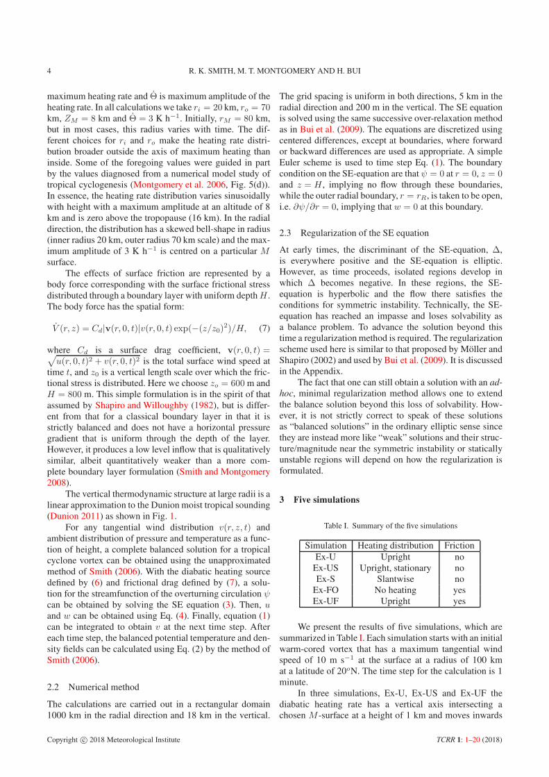
The vertical thermodynamic structure at large radii is a
linear approximation to the Dunion moist tropical sounding
(Dunion 2011) as shown in Fig. 1.
For any tangential wind distribution v(r, z, t) and
ambient distribution of pressure and temperature as a func-
tion of height, a complete balanced solution for a tropical
cyclone vortex can be obtained using the unapproximated
method of Smith (2006). With the diabatic heating source
defined by (6) and frictional drag defined by (7), a solu-
tion for the streamfunction of the overturning circulation ψcan be obtained by solving the SE equation (3). Then, uand w can be obtained using Eq. (4). Finally, equation (1)
can be integrated to obtain v at the next time step. After
each time step, the balanced potential temperature and den-
sity fields can be calculated using Eq. (2) by the method of
Smith (2006).
2.2 Numerical method
The calculations are carried out in a rectangular domain
1000 km in the radial direction and 18 km in the vertical.
The grid spacing is uniform in both directions, 5 km in the
radial direction and 200 m in the vertical. The SE equation
is solved using the same successive over-relaxation method
as in Bui et al. (2009). The equations are discretized using
centered differences, except at boundaries, where forward
or backward differences are used as appropriate. A simple
Euler scheme is used to time step Eq. (1). The boundary
condition on the SE-equation are that ψ = 0 at r = 0, z = 0and z = H , implying no flow through these boundaries,
while the outer radial boundary, r = rR, is taken to be open,
i.e. ∂ψ/∂r = 0, implying that w = 0 at this boundary.
2.3 Regularization of the SE equation
At early times, the discriminant of the SE-equation, ∆,
is everywhere positive and the SE-equation is elliptic.
However, as time proceeds, isolated regions develop in
which ∆ becomes negative. In these regions, the SE-
equation is hyperbolic and the flow there satisfies the
conditions for symmetric instability. Technically, the SE-
equation has reached an impasse and loses solvability as
a balance problem. To advance the solution beyond this
time a regularization method is required. The regularization
scheme used here is similar to that proposed by Moller and
Shapiro (2002) and used by Bui et al. (2009). It is discussed
in the Appendix.
The fact that one can still obtain a solution with an ad-
hoc, minimal regularization method allows one to extend
the balance solution beyond this loss of solvability. How-
ever, it is not strictly correct to speak of these solutions
as “balanced solutions” in the ordinary elliptic sense since
they are instead more like “weak” solutions and their struc-
ture/magnitude near the symmetric instability or statically
unstable regions will depend on how the regularization is
formulated.
3 Five simulations
Table I. Summary of the five simulations
Simulation Heating distribution Friction
Ex-U Upright no
Ex-US Upright, stationary no
Ex-S Slantwise no
Ex-FO No heating yes
Ex-UF Upright yes
We present the results of five simulations, which are
summarized in Table I. Each simulation starts with an initial
warm-cored vortex that has a maximum tangential wind
speed of 10 m s−1 at the surface at a radius of 100 km
at a latitude of 20oN. The time step for the calculation is 1
minute.
In three simulations, Ex-U, Ex-US and Ex-UF the
diabatic heating rate has a vertical axis intersecting a
chosen M -surface at a height of 1 km and moves inwards
Copyright c© 2018 Meteorological Institute TCRR 1: 1–20 (2018)
BALANCE DYNAMICS OF TROPICAL CYCLONE INTENSIFICATION 5
Figure 1. Far field sounding of θ(z) (thick red curve) compared with
that for the Dunion tropical sounding (thin blue curve).
with this M -surface as the vortex evolves. This M -surface,
which corresponds with a potential radius of 265 km, is
located initially inside the radius of maximum tangential
wind speed. The configuration of the simulations Ex-US
and Ex-UF are the same as Ex-U, except that in Ex-US, the
location of the heating distribution is held fixed in space,
while in Ex-UF, a representation of near-surface friction is
included (V 6= 0). In Ex-S, the axis of the diabatic heating
rate is aligned along the chosen M -surface and slopes
upwards and outwards with height, but friction is excluded
(V = 0). The slope of the heating is arguably more realistic
for the mature stage of tropical cyclone development. In
Ex-FO, there is no heating and only friction.
4 Results
4.1 Vortex evolution in the Ex-U calculation
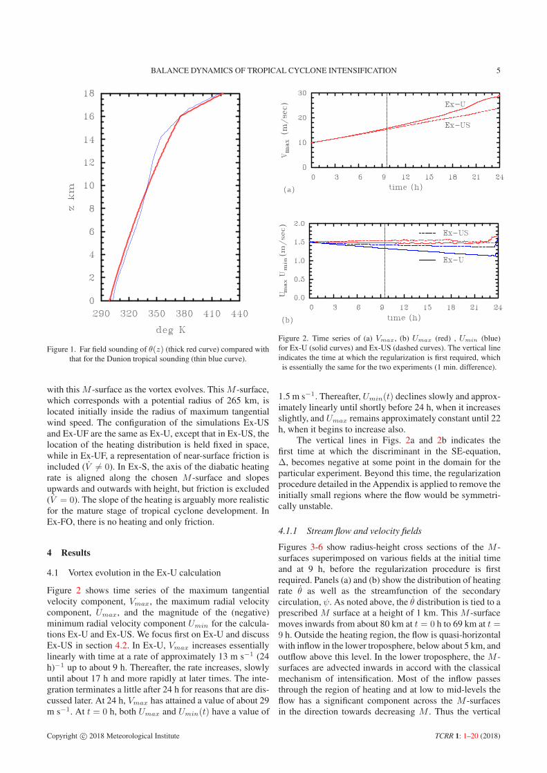
Figure 2 shows time series of the maximum tangential
velocity component, Vmax, the maximum radial velocity
component, Umax, and the magnitude of the (negative)
minimum radial velocity component Umin for the calcula-
tions Ex-U and Ex-US. We focus first on Ex-U and discuss
Ex-US in section 4.2. In Ex-U, Vmax increases essentially
linearly with time at a rate of approximately 13 m s−1 (24
h)−1 up to about 9 h. Thereafter, the rate increases, slowly
until about 17 h and more rapidly at later times. The inte-
gration terminates a little after 24 h for reasons that are dis-
cussed later. At 24 h, Vmax has attained a value of about 29
m s−1. At t = 0 h, both Umax and Umin(t) have a value of
Figure 2. Time series of (a) Vmax, (b) Umax (red) , Umin (blue)
for Ex-U (solid curves) and Ex-US (dashed curves). The vertical line
indicates the time at which the regularization is first required, which
is essentially the same for the two experiments (1 min. difference).
1.5 m s−1. Thereafter, Umin(t) declines slowly and approx-
imately linearly until shortly before 24 h, when it increases
slightly, and Umax remains approximately constant until 22
h, when it begins to increase also.
The vertical lines in Figs. 2a and 2b indicates the
first time at which the discriminant in the SE-equation,
∆, becomes negative at some point in the domain for the
particular experiment. Beyond this time, the regularization
procedure detailed in the Appendix is applied to remove the
initially small regions where the flow would be symmetri-
cally unstable.
4.1.1 Stream flow and velocity fields
Figures 3-6 show radius-height cross sections of the M -
surfaces superimposed on various fields at the initial time
and at 9 h, before the regularization procedure is first
required. Panels (a) and (b) show the distribution of heating
rate θ as well as the streamfunction of the secondary
circulation, ψ. As noted above, the θ distribution is tied to a
prescribed M surface at a height of 1 km. This M -surface
moves inwards from about 80 km at t = 0 h to 69 km at t =9 h. Outside the heating region, the flow is quasi-horizontal
with inflow in the lower troposphere, below about 5 km, and
outflow above this level. In the lower troposphere, the M -
surfaces are advected inwards in accord with the classical
mechanism of intensification. Most of the inflow passes
through the region of heating and at low to mid-levels the
flow has a significant component across the M -surfaces
in the direction towards decreasing M . Thus the vertical
Copyright c© 2018 Meteorological Institute TCRR 1: 1–20 (2018)
6 R. K. SMITH, M. T. MONTGOMERY AND H. BUI
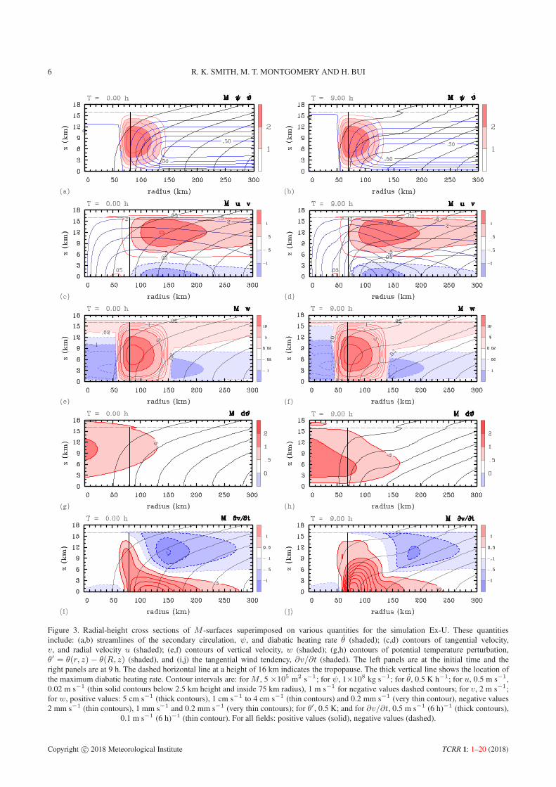
Figure 3. Radial-height cross sections of M -surfaces superimposed on various quantities for the simulation Ex-U. These quantities
include: (a,b) streamlines of the secondary circulation, ψ, and diabatic heating rate θ (shaded); (c,d) contours of tangential velocity,
v, and radial velocity u (shaded); (e,f) contours of vertical velocity, w (shaded); (g,h) contours of potential temperature perturbation,
θ′ = θ(r, z)− θ(R, z) (shaded), and (i,j) the tangential wind tendency, ∂v/∂t (shaded). The left panels are at the initial time and the
right panels are at 9 h. The dashed horizontal line at a height of 16 km indicates the tropopause. The thick vertical line shows the location of
the maximum diabatic heating rate. Contour intervals are: for M , 5 ×10⁵ m2 s−1; for ψ, 1×10⁸ kg s−1; for θ, 0.5 K h−1; for u, 0.5 m s−1,
0.02 m s−1 (thin solid contours below 2.5 km height and inside 75 km radius), 1 m s−1 for negative values dashed contours; for v, 2 m s−1;
for w, positive values: 5 cm s−1 (thick contours), 1 cm s−1 to 4 cm s−1 (thin contours) and 0.2 mm s−1 (very thin contour), negative values
2 mm s−1 (thin contours), 1 mm s−1 and 0.2 mm s−1 (very thin contours); for θ′, 0.5 K; and for ∂v/∂t, 0.5 m s−1 (6 h)−1 (thick contours),
0.1 m s−1 (6 h)−1 (thin contour). For all fields: positive values (solid), negative values (dashed).
Copyright c© 2018 Meteorological Institute TCRR 1: 1–20 (2018)
BALANCE DYNAMICS OF TROPICAL CYCLONE INTENSIFICATION 7
advection of M becomes important in spinning up the
flow there. This behaviour is consistent with the statement
of Pendergrass and Willoughby (2009) (p. 814) that the
acceleration of the tangential wind “is primarily caused
by upward and inward advection of angular momentum”5.
This finding is consistent also with that in a recent study by
Paull et al. (2017).
Panels (c) and (d) of Fig. 3 show the radial and tan-
gential velocity components in relation to the M -surfaces.
The maximum tangential wind speed occurs at the surface
where the inflow is a maximum. This is to be expected
because Vmax lies at the surface initially and Umin occurs
at the surface at subsequent times. Thus, the largest inward
advection of the M -surfaces occurs at the surface. The
asymmetry in the depths of inflow and outflow is a con-
sequence of mass continuity and the fact that density
decreases approximately exponentially with height. The
maximum outflow occurs at a height of about 12 km.
Figures 3e and 3f show the vertical velocity w in
relation to the M -surfaces. At both times shown, there is
strong ascent in the heating region and weak ascent in the
upper troposphere at all radii, except below 13.5 km inside
the heating region. In the lower and middle troposphere,
there is subsidence both inside and outside the heating
region. The maximum vertical velocity is about 18 cm s−1
and it occurs at a height of about 7 km. The subsidence
is strongest at low levels inside the heating region, the
maximum being 4.3 mm s−1 at t = 0. As time proceeds,
the subsidence both inside and outside the heating region
increases in strength as the radius of the heating region
contracts. The maximum subsidence at t = 9 h is 6.4 mm
s−1 and occurs just outside the heating region.
4.1.2 Potential temperature perturbation
Figures 3g and 3h show the perturbation potential temper-
ature, θ′ = θ(r, z)− θ(R, z), relative to the ambient poten-
tial temperature profile at the outer boundary, (r = R). At
t = 0, the warm anomaly in balance with the tangential
wind field has a maximum of 1.1 K located on the rota-
tion axis at an altitude of 10 km. By 9 h, the warm anomaly
has strengthened throughout the vortex core and the maxi-
mum, now 1.4 K, has shifted downwards to 6.2 km, again
on the vortex axis.
4.1.3 Tangential wind tendency
Figures 3i and 3j show the local tangential wind tendency
∂v/∂t, obtained by evaluating the terms on the right hand
side of Eq. (1), which, after rearrangement, represent 1/rtimes the advection of theM -surfaces by the secondary cir-
culation, at least in the present calculation when V = 0. At
both t = 0 h and t = 9 h there is a strong positive tendency
in the lower troposphere within and outside the region of
5These authors made this inference from the fields of balanced tangentialwind tendency, but did not show the structure of the M -surfaces inrelationship to the streamlines.
heating and a tongue extending to the high troposphere
about the axis of heating. This positive tendency, which
coincides with the region where the flow in Fig. 3a and 3b
is across the M surfaces in the direction of decreasing M ,
is a maximum at the surface, but extends through an appre-
ciable depth of the heating region (over 13 km in altitude
at 9 h). The tendency is negative in the upper troposphere,
typically above an altitude of 6 km and mostly beyond the
heating region, where the flow crosses the M surfaces in
the direction of increasing M . This negative tendency is
strongest at levels where the outflow is strong (compare
panels (i) and (j) of Fig. 3 with panels (c) and (d), respec-
tively). At low levels inside the axis of maximum heating
there is a small spin down tendency due to the weak outflow
under the main updraught (see panels (c) and (d)). A similar
pattern of outflow at low levels in the eye region was found
by Pendergrass and Willoughby (2009), see their Fig. 5.
One notable feature at both times is the overlap
between positive tendency and radial outflow, principally
within the upper troposphere in the region of heating (com-
pare again panels (i) and (j) of Fig. 3 with panels (c) and
(d), respectively), but the largest positive tendencies occur
in the lower troposphere where the radial flow is inwards.
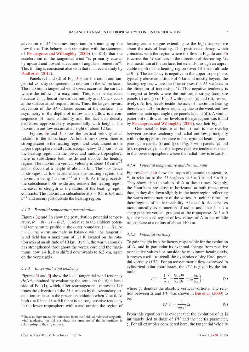
4.1.4 Potential temperature and discriminant
Figures 4a and 4b show isentropes of potential temperature,
θ, in relation to the M -surfaces at t = 0 h and t = 9 h.
They show also the values of ∆ at these times. Notably,
the θ surfaces are close to horizontal at both times, even
though they dip down slightly in the inner region reflecting
the warm core structure of the vortex. At neither times are
there regions of static instability. At t = 0 h, ∆ decreases
monotonically as a function of radius and, like θ, has a
sharp positive vertical gradient at the tropopause. At t = 9h, there is closed region of low values of ∆ in the middle
troposphere at a radius of about 140 km.
4.1.5 Potential vorticity
To gain insight into the factors responsible for the evolution
of ∆, and in particular its eventual change from positive
to negative values just outside the maximum heating axis,
it proves useful to recall the dynamics of dry Ertel poten-
tial vorticity (PV ). For an axisymmetric flow expressed in
cylindrical-polar coordinates, the PV is given by the for-
mula
PV =1
ρ
(
−∂v∂z
∂θ
∂r+ ζa
∂θ
∂z
)
. (8)
where ζa denotes the absolute vertical vorticity. The rela-
tion between ∆ and PV was shown in Bui et al. (2009) to
be:
ξPV =1
ρgχ3∆. (9)
From this equation it is evident that the evolution of ∆ is
intimately tied to those of PV and the inertia parameter,
ξ. For all examples considered here, the tangential velocity
Copyright c© 2018 Meteorological Institute TCRR 1: 1–20 (2018)
8 R. K. SMITH, M. T. MONTGOMERY AND H. BUI
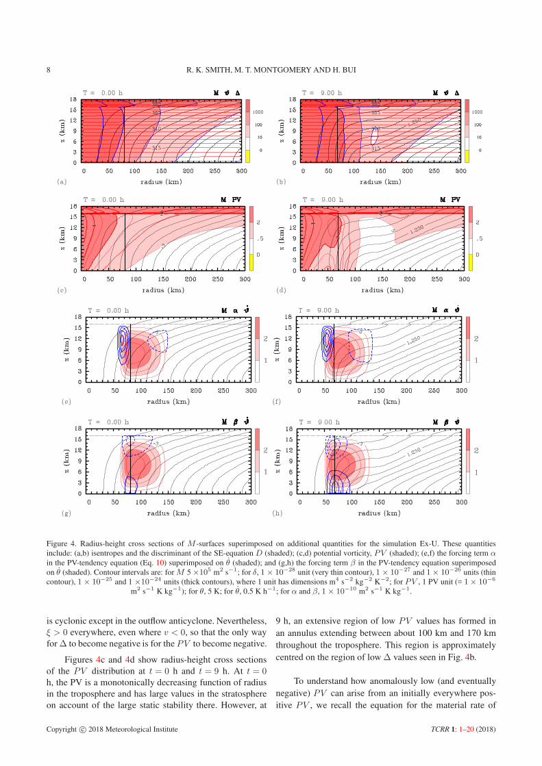
Figure 4. Radius-height cross sections of M -surfaces superimposed on additional quantities for the simulation Ex-U. These quantities
include: (a,b) isentropes and the discriminant of the SE-equation D (shaded); (c,d) potential vorticity, PV (shaded); (e,f) the forcing term αin the PV-tendency equation (Eq. 10) superimposed on θ (shaded); and (g,h) the forcing term β in the PV-tendency equation superimposed
on θ (shaded). Contour intervals are: forM 5 ×10⁵ m2 s−1; for δ, 1× 10⁻²⁸ unit (very thin contour), 1× 10⁻²⁷ and 1× 10⁻²⁶ units (thin
contour), 1× 10⁻²⁵ and 1 ×10⁻²⁴ units (thick contours), where 1 unit has dimensions m4 s−2 kg−2 K−2; for PV , 1 PV unit (= 1× 10⁻⁶
m2 s−1 K kg−1); for θ, 5 K; for θ, 0.5 K h−1; for α and β, 1× 10⁻¹⁰ m2 s−1 K kg−1.
is cyclonic except in the outflow anticyclone. Nevertheless,
ξ > 0 everywhere, even where v < 0, so that the only way
for ∆ to become negative is for the PV to become negative.
Figures 4c and 4d show radius-height cross sections
of the PV distribution at t = 0 h and t = 9 h. At t = 0
h, the PV is a monotonically decreasing function of radius
in the troposphere and has large values in the stratosphere
on account of the large static stability there. However, at
9 h, an extensive region of low PV values has formed in
an annulus extending between about 100 km and 170 km
throughout the troposphere. This region is approximately
centred on the region of low ∆ values seen in Fig. 4b.
To understand how anomalously low (and eventually
negative) PV can arise from an initially everywhere pos-
itive PV , we recall the equation for the material rate of
Copyright c© 2018 Meteorological Institute TCRR 1: 1–20 (2018)
BALANCE DYNAMICS OF TROPICAL CYCLONE INTENSIFICATION 9
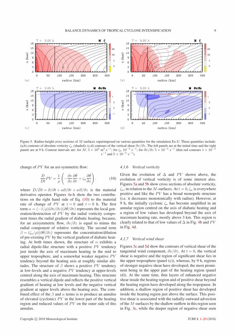
Figure 5. Radius-height cross sections of M -surfaces superimposed on various quantities for the simulation Ex-U. These quantities include:
(a,b) contours of absolute vorticity ζa (shaded); (c,d) contours of the vertical shear ∂v/∂z. The left panels are at the initial time and the right
panels are at 9 h. Contour intervals are: for M , 5× 10⁵ m2 s−1; for ζa 10−5 s−1; for ∂v/∂z 5× 10⁻⁵ s−1 (thin red contours 1× 10⁻⁵
s−1 and 5× 10⁻⁵ s−1).
change of PV for an axi-symmetric flow:
D
DtPV =
1
ρ
(
−∂v∂z
∂θ
∂r+ ζa
∂θ
∂z
)
. (10)
where D/Dt = ∂/∂t+ u∂/∂r + w∂/∂z is the material
derivative operator. Figures 4e-h show the two contribu-
tions on the right hand side of Eq. (10) to the material
rate of change of PV at t = 0 and t = 9 h. The first
term α = (−1/ρ)(∂v/∂z)(∂θ/∂r) represents the local gen-
eration/destruction of PV by the radial vorticity compo-
nent times the radial gradient of diabatic heating, because,
for an axisymmetric flow, ∂v/∂z is equal to minus the
radial component of relative vorticity. The second term
β = (ζa/ρ)(∂θ/∂z) represents the concentration/dilution
of pre-existing PV by the vertical gradient of diabatic heat-
ing. At both times shown, the structure of α exhibits a
radial dipole-like structure with a positive PV tendency
just inside the axis of maximum heating in the mid to
upper troposphere, and a somewhat weaker negative PVtendency beyond the heating axis at roughly similar alti-
tudes. The structure of β shows a positive PV tendency
at low-levels and a negative PV tendency at upper-levels
centred along the axis of maximum heating. This structure
resembles a vertical dipole and reflects the positive vertical
gradient of heating at low levels and the negative vertical
gradient at upper levels above the heating axis. The com-
bined effect of the β and α terms is to produce an annulus
of elevated (cyclonic) PV in the lower part of the heating
region and reduced values of PV on the outer side of this
annulus.
4.1.6 Vertical vorticity
Given the evolution of ∆ and PV shown above, the
evolution of vertical vorticity is of some interest also.
Figures 5a and 5b show cross sections of absolute vorticity,
ζa, in relation to theM -surfaces. At t = 0, ζa is everywhere
positive and like the PV has a broad monopole structure
(i.e. it decreases monotonically with radius). However, at
9 h, the initially cyclonic ζa has become amplified in an
annular region centred on the axis of diabatic heating and
a region of low values has developed beyond the axis of
maximum heating rate, mostly above 3 km. This region is
clearly related to that of low values of ∆ in Fig. 4b and PVin Fig. 4d.
4.1.7 Vertical wind shear
Figures 5c and 5d show the contours of vertical shear of the
tangential wind component, ∂v/∂z. At t = 0, the vertical
shear is negative and the region of significant shear lies in
the upper troposphere (panel (c)), whereas, by 9 h, regions
of stronger negative shear have developed, the most promi-
nent being in the upper part of the heating region (panel
(d)). At the same time, thin layers of enhanced negative
shear inside the heating region and of positive shear beyond
the heating region have developed along the tropopause. In
addition, a shallow region of positive shear has developed
inside the heating region just above the surface. This posi-
tive shear is associated with the radially-outward advection
of theM -surfaces by the shallow outflow in this region seen
in Fig. 3c, while the deeper region of negative shear seen
Copyright c© 2018 Meteorological Institute TCRR 1: 1–20 (2018)
10 R. K. SMITH, M. T. MONTGOMERY AND H. BUI
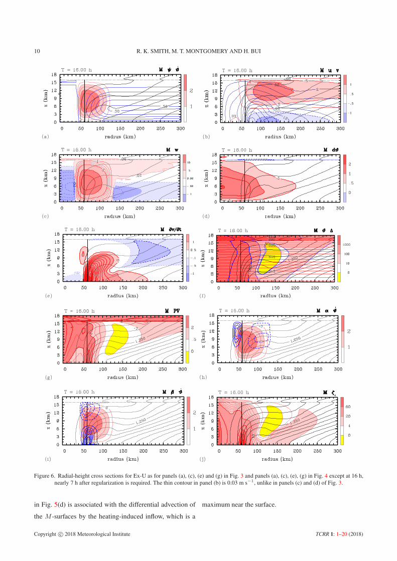
Figure 6. Radial-height cross sections for Ex-U as for panels (a), (c), (e) and (g) in Fig. 3 and panels (a), (c), (e), (g) in Fig. 4 except at 16 h,
nearly 7 h after regularization is required. The thin contour in panel (b) is 0.03 m s−1, unlike in panels (c) and (d) of Fig. 3.
in Fig. 5(d) is associated with the differential advection of
the M -surfaces by the heating-induced inflow, which is a
maximum near the surface.
Copyright c© 2018 Meteorological Institute TCRR 1: 1–20 (2018)
BALANCE DYNAMICS OF TROPICAL CYCLONE INTENSIFICATION 11
4.1.8 Development of symmetrically-unstable regions
Figure 6 shows radius-height cross sections of selected
quantities similar to those in Figs. 3-5, but at 16 h, more
than 6 h after a region of symmetric instability has devel-
oped and the SE-equation requires regularization. Even at
this time, the fields are generally smooth. The axis of heat-
ing has moved further inwards to just over 60 km radius and
some of the M surfaces have folded in the mid and upper
troposphere to form a “well-like” structure beyond the heat-
ing region, partly because of differential vertical advection
of theM -surfaces between the ascending branch of the sec-
ondary circulation and the region of subsidence outside the
heating. Some distance inwards from the lowest point of
the well, the radial gradient of M is negative, implying
negative absolute vorticity and thereby inertial instability.
It is interesting that, even at this stage of evolution, the M -
surfaces are generally not congruent with the streamlines in
the upper troposphere as they would have to be if the flow
were close to a steady state.
Notably, the subsidence inside the heating region has
strengthened (panel (c)) and the eye has warmed further
(panel (d)), θ′ now being 2 K at a height of 5.8 km
compared with 1.4 K at a height of 6.2 km at 9 h. The
tangential wind tendency has increased further and remains
positive at the location of Vmax (compare panels (e) and
(b)) consistent with the continued increase in Vmax seen in
Fig. 2. Positive tendencies in the region of heating continue
to extend above 11 km and at larger heights, these positive
tendencies overlap with regions of outflow, highlighting the
importance of the vertical advection on M in spinning up
this region.
At 16 h, the regions of low ∆, PV and ζa seen in Figs.
4 and 5 have become more pronounced and regions where
these quantities are negative have formed (Figs. 6f, 6g and
6j). As noted above, the region of negative ζa coincides
with that in which theM -surfaces dip down with increasing
radius and because the static stability does not reverse
sign anywhere (panel(f)), the region of inertial instability
is one also of symmetric instability in which both ∆ and
PV are negative. Panels (h) and (i) of Fig. 6 show similar
patterns of PV generation as in panels (e), (f) and (g), (h),
respectively, of Fig. 4. Because, in the absence of heating,
PV is materially conserved, the occurrence of regions of
negative PV must be a result of the negative generation
of PV in the upper troposphere, which is another way of
viewing the formation of a region of symmetric instability.
4.1.9 Ultimate solution breakdown
The breakdown of the regularized solution shortly after 24
h is brought about by the appearance and growth of small-
scale features in the secondary circulation in the upper tro-
posphere, near the edge of where ∆ < 0 (not shown). The
small-scale features arise from spatial irregularities intro-
duced by the ad-hoc regularization method described in
the Appendix. This regularization procedure is necessarily
somewhat arbitrary and only removes conditions for sym-
metric instability in the SE-equation and not in the equation
for the tangential wind tendency. As a result, regions of
inertial instability with negative values of ζa are still seen
by the tendency equation and inertial instability can still
manifest itself during the flow evolution. Typically, regions
of static instability occur only in the presence of friction
and with our method here, they tend to lead to a catastrophic
breakdown of the solution very rapidly.
Eventually, a time is reached when M becomes neg-
ative at some point, presumably on account of numerical
issues. At this point, the solution is programmed to ter-
minate. While it may be possible to extend the solution
beyond this point for some time interval by refining the
numerical algorithm (and in part smoothing the coefficients
in the SE-equation after each regularization step), the main
purpose of our study is to understand how the axisymmet-
ric balance solution, itself, breaks down and not to devise
necessarily ad hoc ways to extend the solution.
If, for the sake of argument, such a continuation
method could be developed, we would expect to see con-
tinued sharpening of the radial gradient of M at the base
of the updraught as air is drawn into the updraught from
both sides near the surface. In essence, the flow there
is trying to form a discontinuity in M (and a corre-
sponding vortex sheet) by a process akin to frontogenesis
(Hoskins and Bretherton 1972, Emanuel 1997).
However, even if one could prolong the period in
which the regularized solution could be obtained, in the
presence of non-axisymmetric perturbations, one would
expect that the annular vortex sheet would be baro-
clinically unstable on account of the reversal in sign
of the radial and vertical gradient of the axisymmetric
PV (Montgomery and Shapiro 1995, Schubert et al. 1999,
Naylor and Schecter 2014). Questions concerning these
and other non-axisymmetric instabilities of the vorticity
annulus, as well as longer-term evolution issues, lie beyond
the scope of the current study. The reader is referred to
Naylor and Schecter (2014), Menelaou et al. (2016), and
references cited therein, for further analysis and discussion
of these complex topics.
4.1.10 Uniform intensification rate
An interesting feature of the foregoing solution worth
remarking on is the approximately uniform intensification
rate, at least before regularization of the SE-equation is
required6. Even beyond that time, there is only a relatively
slow increase in spin up as the vortex intensity increases.
This finding, which is a feature of all the calculations
6We remind the reader that we use the term “intensification rate” for thechange in the maximum tangential wind speed and not the maximum inthe tendency at any point, as the location of these maxima do not, ingeneral, coincide. Thus although the maximum tendency approximatelydoubles between Fig.3(i) and 3(j), this doubling does not occur at thelocation of Vmax.
Copyright c© 2018 Meteorological Institute TCRR 1: 1–20 (2018)
12 R. K. SMITH, M. T. MONTGOMERY AND H. BUI
forced by heating shown below, differs from some previ-
ous inferences based on balance theory that the intensifica-
tion rate should increase as the vortex intensifies because
the heating becomes progressively more efficient (Vigh
and Schubert 2009 and refs.). An appraisal of ideas relat-
ing the efficiency of diabatic heating to the inertial stabil-
ity is given by Smith and Montgomery (2016b): see also
(Kilroy and Smith, 2016, section 7).
We cannot regard the finding of an approximately
uniform intensification rate as general, of course, because
of the limited number of simulations we have carried out
and because the solutions break down at wind speeds
approaching minimal hurricane intensity. Most previous
theories fix the structure of both the heating rate and the
vortex and diagnose the intensification rate at individual
times as a function of vortex intensity. In contrast, the
present approach is to integrate the balance equations as
an initial-value problem so that the vortex structure and,
in most experiments the location, but not the structure
of the heating, evolve with time. In the experiments with
imposed heating, an annulus of cyclonic PV of limited
radial extent is generated around the heating region. Thus,
prior calculations that assume an increase in vorticity
across the entire inner-core would over-estimate the extent
of the vorticity increase in comparison. The occurrence of
the approximately constant intensification rate found here
may be influenced also, in part, by the change in location
of the heating relative to the axis of rotation, because the
spatial gradients of the heating, and therefore the magnitude
of the diabatic forcing term in the SE-equation does not
change (see Equation (11) in the appendix).
4.2 Vortex evolution in the Ex-US calculation
Ex-US is similar to Ex-U, but the axis of heating is held
fixed, as for example in the calculations by Heng and Wang
(2016). The Ex-US simulation is carried out as a bench-
mark to examine the consequences of allowing the heating
axis to move in the Ex-U simulation. Time series of Vmax,
Umax and Umin for this experiment are included in Fig. 2
and show, perhaps as expected, that intensification rate is
impeded in this case. However, there is little difference in
the Vmax curves until after the time when the SE-equation
requires regularization, which is merely a minute later
in Ex-US. Notwithstanding the previous caveat, a likely
reason for the reduced intensification rate is because only
those M -surfaces within and beyond the region of heat-
ing can be drawn inwards by the heating-induced secondary
circulation and the radius to which a given M -surface can
be drawn inwards is thereby limited.
The maximum inflow becomes fractionally larger in
Ex-US, presumably on account of the slightly weaker
vortex, which provides a reduced inertial stability and
hence less resistance to radial parcel displacements.
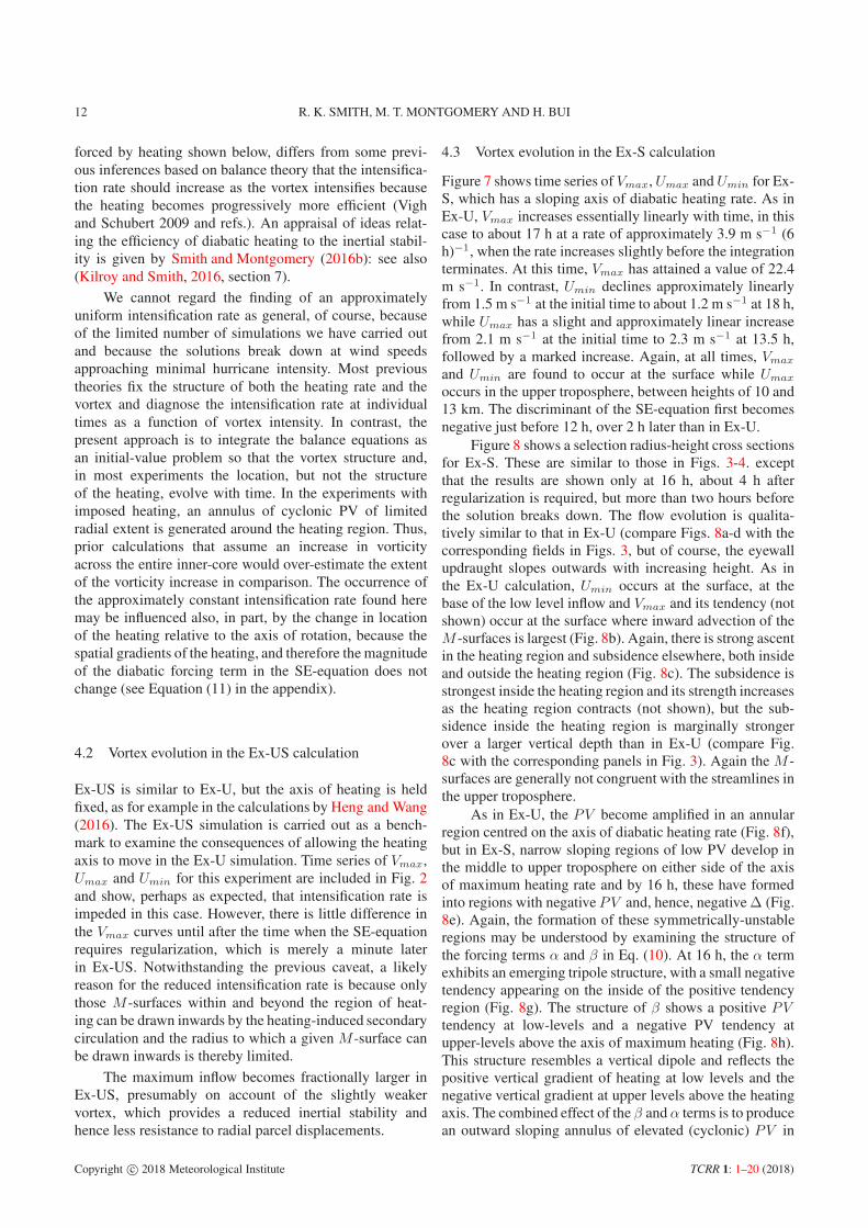
4.3 Vortex evolution in the Ex-S calculation
Figure 7 shows time series of Vmax,Umax and Umin for Ex-
S, which has a sloping axis of diabatic heating rate. As in
Ex-U, Vmax increases essentially linearly with time, in this
case to about 17 h at a rate of approximately 3.9 m s−1 (6
h)−1, when the rate increases slightly before the integration
terminates. At this time, Vmax has attained a value of 22.4
m s−1. In contrast, Umin declines approximately linearly
from 1.5 m s−1 at the initial time to about 1.2 m s−1 at 18 h,
while Umax has a slight and approximately linear increase
from 2.1 m s−1 at the initial time to 2.3 m s−1 at 13.5 h,
followed by a marked increase. Again, at all times, Vmax
and Umin are found to occur at the surface while Umax
occurs in the upper troposphere, between heights of 10 and
13 km. The discriminant of the SE-equation first becomes
negative just before 12 h, over 2 h later than in Ex-U.
Figure 8 shows a selection radius-height cross sections
for Ex-S. These are similar to those in Figs. 3-4. except
that the results are shown only at 16 h, about 4 h after
regularization is required, but more than two hours before
the solution breaks down. The flow evolution is qualita-
tively similar to that in Ex-U (compare Figs. 8a-d with the
corresponding fields in Figs. 3, but of course, the eyewall
updraught slopes outwards with increasing height. As in
the Ex-U calculation, Umin occurs at the surface, at the
base of the low level inflow and Vmax and its tendency (not
shown) occur at the surface where inward advection of the
M -surfaces is largest (Fig. 8b). Again, there is strong ascent
in the heating region and subsidence elsewhere, both inside
and outside the heating region (Fig. 8c). The subsidence is
strongest inside the heating region and its strength increases
as the heating region contracts (not shown), but the sub-
sidence inside the heating region is marginally stronger
over a larger vertical depth than in Ex-U (compare Fig.
8c with the corresponding panels in Fig. 3). Again the M -
surfaces are generally not congruent with the streamlines in
the upper troposphere.
As in Ex-U, the PV become amplified in an annular
region centred on the axis of diabatic heating rate (Fig. 8f),
but in Ex-S, narrow sloping regions of low PV develop in
the middle to upper troposphere on either side of the axis
of maximum heating rate and by 16 h, these have formed
into regions with negative PV and, hence, negative ∆ (Fig.
8e). Again, the formation of these symmetrically-unstable
regions may be understood by examining the structure of
the forcing terms α and β in Eq. (10). At 16 h, the α term
exhibits an emerging tripole structure, with a small negative
tendency appearing on the inside of the positive tendency
region (Fig. 8g). The structure of β shows a positive PVtendency at low-levels and a negative PV tendency at
upper-levels above the axis of maximum heating (Fig. 8h).
This structure resembles a vertical dipole and reflects the
positive vertical gradient of heating at low levels and the
negative vertical gradient at upper levels above the heating
axis. The combined effect of the β and α terms is to produce
an outward sloping annulus of elevated (cyclonic) PV in
Copyright c© 2018 Meteorological Institute TCRR 1: 1–20 (2018)
BALANCE DYNAMICS OF TROPICAL CYCLONE INTENSIFICATION 13
Figure 7. Time series of (a) Vmax, (b) Umax, Umin for Ex-S. The dashed vertical line indicates the time at which the regularization is first
required.
the main updraught, with reduced values of PV on both
sides of the annulus.
Panel (i) of Fig. 8 shows the tangential wind tendency
in Ex-S at 16 h, which has a slightly different structure to
that in Fig. 6e with the appearance of a tongue of strong
spin down tendency on the upper side of the heating axis.
However, below this axis, there is a region of strong positive
tendency extending to above 11 km as in the calculations
with upright heating distributions. Again, this positive ten-
dency may be attributed to the vertical advection of M and
it occurs in a region where there is predominantly outflow.
Finally, the complete breakdown of the solution is due
to the appearance and growth of small-scale features in the
secondary circulation in the upper troposphere, near the
edge of where ∆ < 0 and the solution is terminated when
the potential radius becomes negative at some grid point
(not shown).
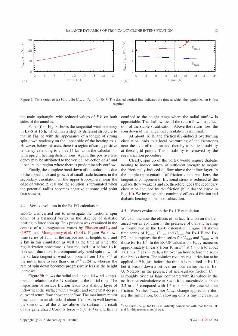
4.4 Vortex evolution in the Ex-FO calculation
Ex-FO was carried out to investigate the frictional spin
down of a balanced vortex in the absence of diabatic
heating to force spin up. This problem was examined in the
context of a homogeneous vortex by Eliassen and Lystad
(1977) and Montgomery et al. (2001). Figure 9a shows
time series of Vmax at the surface and at heights of 1 and
2 km in this simulation as well as the time at which the
regularization procedure is first required just before 16 h.
It is seen that there is a comparatively rapid spin down of
the surface tangential wind component from 10 m s−1 at
the initial time to less than 6 m s−1 at 24 h, whereas the
rate of spin down becomes progressively less as the height
increases.
Figure 9b shows the radial and tangential wind compo-
nents in relation to the M -surfaces at the initial time. The
imposition of surface friction leads to a shallow layer of
inflow near the surface with a weaker and somewhat deeper
outward return flow above the inflow. The maximum return
flow occurs at an altitude of about 1 km. As is well known,
the spin down of the vortex above the surface is a result
of the generalized Coriolis force −(v/r + f)u and this is
confined to the height range where the radial outflow is
appreciable. The shallowness of the return flow is a reflec-
tion of the stable stratification. Above the return flow, the
spin down of the tangential circulation is minimal.
At about 16 h, the frictionally-induced overturning
circulation leads to a local overturning of the isentropes
near the axis of rotation and thereby to static instability
at these grid points. This instability is removed by the
regularization procedure.
Clearly, spin up of the vortex would require diabatic
heating to induce inflow of sufficient strength to negate
the frictionally-induced outflow above the inflow layer. In
the simple representation of friction considered here, the
tangential component of frictional stress is reduced as the
surface flow weakens and so, therefore, does the secondary
circulation induced by the friction (blue dashed curve in
Fig. 10). We investigate the combined effects of friction and
diabatic heating in the next subsection.
4.5 Vortex evolution in the Ex-UF calculation
We examine now the effects of surface friction on the bal-
anced vortex evolution in the presence of diabatic heating
as formulated in the Ex-U calculation. Figure 10 shows
time series of Vmax, Umax and Umin for Ex-UF and Ex-
FO and compares the time series for Vmax and Umin with
those for Ex-U7. In the Ex-UF calculation, Vmax increases
approximately linearly from 10 m s−1 at t = 0 h to about
17.1 m s−1 at t = 24 h, a bit over an hour before the solu-
tion breaks down. The solution requires regularization to be
applied at 9 h, just before the time it is required in Ex-U,
but it breaks down a bit over an hour earlier than in Ex-
U. Notably, in the presence of near-surface friction Umin
is roughly twice as large compared with its values in the
no friction calculations: at t = 0 h its magnitude is about
3.2 m s−1 compared with 1.5 m s−1 in the case without
friction. Neither Umin nor Umax change appreciably dur-
ing the simulation, both showing only a tiny increase. In
7The curve Umax for Ex-U is virtually coincident with that for Ex-UFand for this reason is not shown.
Copyright c© 2018 Meteorological Institute TCRR 1: 1–20 (2018)
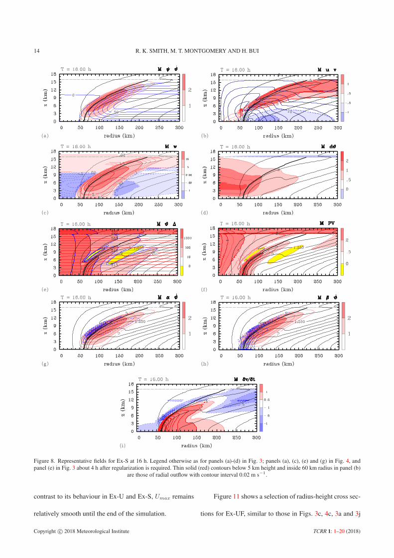
14 R. K. SMITH, M. T. MONTGOMERY AND H. BUI
Figure 8. Representative fields for Ex-S at 16 h. Legend otherwise as for panels (a)-(d) in Fig. 3; panels (a), (c), (e) and (g) in Fig. 4, and
panel (e) in Fig. 3 about 4 h after regularization is required. Thin solid (red) contours below 5 km height and inside 60 km radius in panel (b)
are those of radial outflow with contour interval 0.02 m s−1.
contrast to its behaviour in Ex-U and Ex-S, Umax remains
relatively smooth until the end of the simulation.
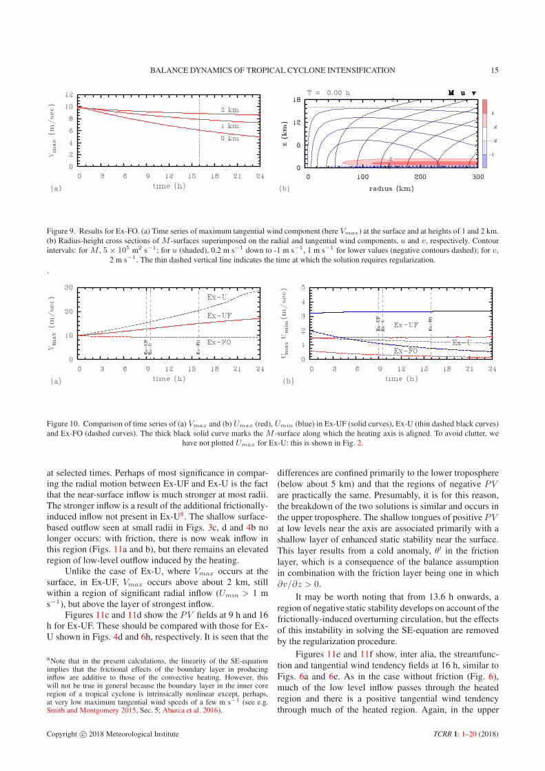
Figure 11 shows a selection of radius-height cross sec-
tions for Ex-UF, similar to those in Figs. 3c, 4c, 3a and 3j
Copyright c© 2018 Meteorological Institute TCRR 1: 1–20 (2018)
BALANCE DYNAMICS OF TROPICAL CYCLONE INTENSIFICATION 15
Figure 9. Results for Ex-FO. (a) Time series of maximum tangential wind component (here Vmax) at the surface and at heights of 1 and 2 km.
(b) Radius-height cross sections of M -surfaces superimposed on the radial and tangential wind components, u and v, respectively. Contour
intervals: for M , 5× 10⁵ m2 s−1; for u (shaded), 0.2 m s−1 down to -1 m s−1, 1 m s−1 for lower values (negative contours dashed); for v,
2 m s−1. The thin dashed vertical line indicates the time at which the solution requires regularization.
.
Figure 10. Comparison of time series of (a) Vmax and (b) Umax (red), Umin (blue) in Ex-UF (solid curves), Ex-U (thin dashed black curves)
and Ex-FO (dashed curves). The thick black solid curve marks the M -surface along which the heating axis is aligned. To avoid clutter, we
have not plotted Umax for Ex-U: this is shown in Fig. 2.
at selected times. Perhaps of most significance in compar-
ing the radial motion between Ex-UF and Ex-U is the fact
that the near-surface inflow is much stronger at most radii.
The stronger inflow is a result of the additional frictionally-
induced inflow not present in Ex-U8. The shallow surface-
based outflow seen at small radii in Figs. 3c, d and 4b no
longer occurs: with friction, there is now weak inflow in
this region (Figs. 11a and b), but there remains an elevated
region of low-level outflow induced by the heating.
Unlike the case of Ex-U, where Vmax occurs at the
surface, in Ex-UF, Vmax occurs above about 2 km, still
within a region of significant radial inflow (Umin > 1 m
s−1), but above the layer of strongest inflow.
Figures 11c and 11d show the PV fields at 9 h and 16
h for Ex-UF. These should be compared with those for Ex-
U shown in Figs. 4d and 6h, respectively. It is seen that the
8Note that in the present calculations, the linearity of the SE-equationimplies that the frictional effects of the boundary layer in producinginflow are additive to those of the convective heating. However, thiswill not be true in general because the boundary layer in the inner coreregion of a tropical cyclone is intrinsically nonlinear except, perhaps,at very low maximum tangential wind speeds of a few m s−1 (see e.g.Smith and Montgomery 2015, Sec. 5; Abarca et al. 2016).
differences are confined primarily to the lower troposphere
(below about 5 km) and that the regions of negative PVare practically the same. Presumably, it is for this reason,
the breakdown of the two solutions is similar and occurs in
the upper troposphere. The shallow tongues of positive PVat low levels near the axis are associated primarily with a
shallow layer of enhanced static stability near the surface.
This layer results from a cold anomaly, θ′ in the friction
layer, which is a consequence of the balance assumption
in combination with the friction layer being one in which
∂v/∂z > 0.
It may be worth noting that from 13.6 h onwards, a
region of negative static stability develops on account of the
frictionally-induced overturning circulation, but the effects
of this instability in solving the SE-equation are removed
by the regularization procedure.
Figures 11e and 11f show, inter alia, the streamfunc-
tion and tangential wind tendency fields at 16 h, similar to
Figs. 6a and 6e. As in the case without friction (Fig. 6),
much of the low level inflow passes through the heated
region and there is a positive tangential wind tendency
through much of the heated region. Again, in the upper
Copyright c© 2018 Meteorological Institute TCRR 1: 1–20 (2018)
16 R. K. SMITH, M. T. MONTGOMERY AND H. BUI
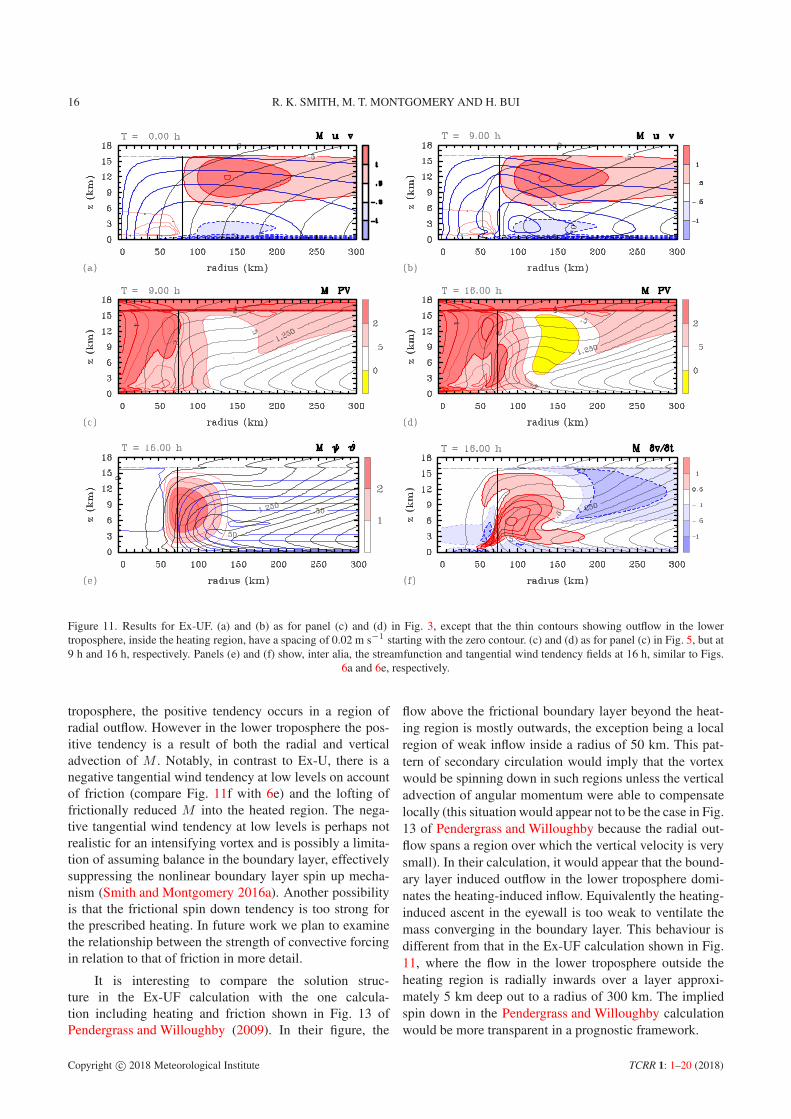
Figure 11. Results for Ex-UF. (a) and (b) as for panel (c) and (d) in Fig. 3, except that the thin contours showing outflow in the lower
troposphere, inside the heating region, have a spacing of 0.02 m s−1 starting with the zero contour. (c) and (d) as for panel (c) in Fig. 5, but at
9 h and 16 h, respectively. Panels (e) and (f) show, inter alia, the streamfunction and tangential wind tendency fields at 16 h, similar to Figs.
6a and 6e, respectively.
troposphere, the positive tendency occurs in a region of
radial outflow. However in the lower troposphere the pos-
itive tendency is a result of both the radial and vertical
advection of M . Notably, in contrast to Ex-U, there is a
negative tangential wind tendency at low levels on account
of friction (compare Fig. 11f with 6e) and the lofting of
frictionally reduced M into the heated region. The nega-
tive tangential wind tendency at low levels is perhaps not
realistic for an intensifying vortex and is possibly a limita-
tion of assuming balance in the boundary layer, effectively
suppressing the nonlinear boundary layer spin up mecha-
nism (Smith and Montgomery 2016a). Another possibility
is that the frictional spin down tendency is too strong for
the prescribed heating. In future work we plan to examine
the relationship between the strength of convective forcing
in relation to that of friction in more detail.
It is interesting to compare the solution struc-
ture in the Ex-UF calculation with the one calcula-
tion including heating and friction shown in Fig. 13 of
Pendergrass and Willoughby (2009). In their figure, the
flow above the frictional boundary layer beyond the heat-
ing region is mostly outwards, the exception being a local
region of weak inflow inside a radius of 50 km. This pat-
tern of secondary circulation would imply that the vortex
would be spinning down in such regions unless the vertical
advection of angular momentum were able to compensate
locally (this situation would appear not to be the case in Fig.
13 of Pendergrass and Willoughby because the radial out-
flow spans a region over which the vertical velocity is very
small). In their calculation, it would appear that the bound-
ary layer induced outflow in the lower troposphere domi-
nates the heating-induced inflow. Equivalently the heating-
induced ascent in the eyewall is too weak to ventilate the
mass converging in the boundary layer. This behaviour is
different from that in the Ex-UF calculation shown in Fig.
11, where the flow in the lower troposphere outside the
heating region is radially inwards over a layer approxi-
mately 5 km deep out to a radius of 300 km. The implied
spin down in the Pendergrass and Willoughby calculation
would be more transparent in a prognostic framework.
Copyright c© 2018 Meteorological Institute TCRR 1: 1–20 (2018)
BALANCE DYNAMICS OF TROPICAL CYCLONE INTENSIFICATION 17
The foregoing comparison points to limitations of per-
forming diagnostic calculations by themselves as opposed
to an integration of an initial value problem. For example,
Pendergrass and Willoughby’s vortices have maximum tan-
gential velocities of 50 m s−1, whereas in all the present
prognostic balance calculations starting with a tangential
wind maximum of 10 m s−1, breakdown of the solu-
tions occurs at maximum wind speeds close to 30 m s−1.
Notwithstanding the fact that the prognostic system may
have its own limitations, this finding raises the possi-
bility that not all strong vortices used as starting points
for diagnostic calculations may be attainable from path-
ways involving balanced evolution from an initial vortex
of only modest intensity. Clearly, further work is required
to explore this possibility.
5 Discussion and conclusions
The axisymmetric balance model calculations presented
herein provide a benchmark for understanding the clas-
sical spin up mechanism for tropical cyclone intensifica-
tion, which refers to the convectively-induced inward radial
advection of absolute angular momentum (M ) at levels
where this quantity is materially conserved. The role of
this mechanism in the spin up of the eyewall (the heating
region) was investigated for a range of heating configura-
tions, both in an inviscid model and one with a balanced
frictional boundary layer. It was shown that, beyond the
heating region, the flow is quasi-horizontal and spins up
by the classical mechanism. Much of the heating-induced
inflow ascends in the heating region and flows outwards
in the upper troposphere. In the lower half of the heating
region, the secondary circulation has a local component
of flow both inwards and upwards across the M -surfaces
towards low values of M , i.e. the vertical advection of Mbecomes important in spinning uresults from previous stud-
iesresults from previous studiesp the eyewall. In the upper
part of the eyewall, positive tangential wind tendencies are
found in regions of radial outflow and in these regions, the
vertical advection of M is the dominant spin up process.
In the cases without friction, there is weak outflow
at low levels inside the annulus of heating as well as
inflow beyond this annulus. This deformation flow pattern,
in the presence of a radial gradient of M , leads to a
spatial concentration of M -surfaces near this axis. The
effect is akin to a frontogenesis process with M serving
as the frontogenetic element. This process tends toward a
discontinuity in M and amplifies the vorticity towards a
vortex sheet. Whether this vortex sheet materializes in a
finite time remains an open question in general, but can be
expected to depend on the chosen parameters in the model.
In all the flows with heating, the vortex intensification
rate hardly changes, at least before appreciable regions of
symmetric instability have developed. This finding does
not support the idea that spin-up increases markedly as the
vortex intensity increases, a finding that is in contrast to
some previous results. However, as discussed in the text,
there are some differences in the formulation of the present
model and previous ones and the integrations only reach
minimal hurricane intensity before they break down so that
general conclusions from this finding cannot be drawn.
The axisymmetric balance solutions can be integrated
only for a finite time before the discriminant (and poten-
tial vorticity) of the SE-equation becomes negative and a
regularization procedure becomes necessary to keep the
equation globally elliptic. Beyond this time, the solutions
eventually become noisy in the upper troposphere as the
regions with negative discriminant before regularization
become larger in size. The integrity of the solutions after
the discriminant (and potential vorticity) becomes appre-
ciably negative is unclear, in part because of the expectation
that symmetric instability will occur at small-scale (e.g.
Thorpe and Rotunno 1989) and also because of hydrody-
namic shear instability and mesovortices that are expected
to develop on the emerging vortex sheet on the inside of
the eyewall (Montgomery et al. 2002, Naylor and Schecter
2014, and refs.). Furthermore, it does not appear that the
streamlines and M -surfaces are becoming congruent in the
upper troposphere on the time-scale over which the solu-
tions break down, calling into question the existence of a
quasi-steady state, even in the inner-core region. This find-
ing would appear to have implications for assumed steady
state models such as that of Emanuel (1986) and later incar-
nations thereof (e.g. Emanuel 2012).
The work described herein was motivated in part by
the desire to understand how the tropical cyclone eyewall
spins up in numerical model simulations and in the real
atmosphere if the air within the eyewall has a radially-
outward component after leaving the boundary layer. A
related question is whether the classical paradigm for
tropical cyclone intensification can be utilized in such
an explanation. Exemplified by the range of calculations
carried out, it would appear that the classical paradigm for
intensification cannot explain the spin up of the eyewall in
the lower troposphere if the air within the eyewall is moving
radially outwards. In all the calculations shown, spin up of
the lower portion of the eyewall occurs by the classical
mechanism in conjunction with the vertical advection of
M . In the calculation with boundary layer friction, spin
down occurs in the friction layer. Nevertheless, in the upper
part of the heating region, there are regions where the
vertical advection of M is sufficiently large that a positive
spin up tendency occurs even in regions of radial outflow.
In a strictly axisymmetric balanced model (see foot-
note 2), or in a generalized balanced flow consisting of gra-
dient wind balance above the boundary layer and Ekman-
like balance in the boundary layer (e.g. Abarca et al. 2015),
the vertical gradient of M in the boundary layer is posi-
tive. Clearly, for sustained spin up to occur anywhere where
there is radial outflow, there are two possibilities. Either
there must be a sufficiently-large negative vertical gradient
ofM above the boundary layer to permit the vertical advec-
tion of M to dominate the spin down tendency accompany-
ing radial advection, or there must be a source of high M
Copyright c© 2018 Meteorological Institute TCRR 1: 1–20 (2018)
18 R. K. SMITH, M. T. MONTGOMERY AND H. BUI
in the boundary layer. There may, of course be a temporary
spin up depending on the structure of the initial vortex, but
without a low-level source of M , by for example the clas-
sical mechanism or from the boundary layer, the spin up
cannot be maintained.
It has been shown in recent work that, in an axisym-
metric configuration, the spin up of supergradient tangen-
tial winds in the boundary layer can provide the neces-
sary negative vertical gradient of M to spin up the eyewall
(Schmidt and Smith 2016, Persing et al. 2013, Fig. 12(d)).
However, in a three-dimensional configuration, there is evi-
dence that the spin up of the eyewall in the lower tropo-
sphere is accomplished by resolved eddy momentum fluxes
(Persing et al. 2013, cf .Fig. 10(d), (g) and (h); Kilroy 2018,
personal communication).
6 Appendix
The SE-equation, Eq. (3) may be written in the form:
∂
∂r
[
A∂ψ
∂r+
1
2B∂ψ
∂z
]
+∂
∂z
[
C∂ψ
∂z+
1
2B∂ψ
∂r
]
= Θ,
(11)
where
A = −g ∂χ∂z
1
ρr=
(
χ
ρr
)
N2,
B = − 2
ρr
∂
∂z(χC) = − 2
ρr
(
χξ∂v
∂z+ C
∂χ
∂z
)
,
C =
(
ξ(ζ + f)χ+ C∂χ
∂r
)
1
ρr= χI2g ,
and
Θ = g∂
∂r
(
χ2θ)
+∂
∂z
(
Cχ2θ)
+ g∂Fλ
∂r+
∂
∂z(χξFλ) ,
where N is the Brunt-Vaisala frequency defined as
(g/θ)∂θ/∂z and I is the generalized inertial frequency
defined by I2 = ξ(ζ + f) + Cχ
∂χ∂r
. It follows that A and Ccharacterize the static stability and inertial stability, respec-
tively. Further, B characterizes, in part, the strength of the
vertical shear.
Equation (11) may be written alternatively as:
A∂2ψ
∂r2+ B
∂2ψ
∂z∂r+ C
∂2ψ
∂z2+ E
∂ψ
∂r+ F
∂ψ
∂z= Θ, (12)
where
E =∂A
∂r+
1
2
∂B
∂z,
and
F =∂C
∂z+
1
2
∂B
∂r.
Equation (12) is an elliptic equation provided that the
discriminant, ∆ = 4AC − B2 > 0. For a vortex that is both
statically stable and inertially stable, N2 and I2 are both
positive and provided that the vertical shear is not too large,
the criterion for ellipticity is everywhere satisfied.Typically,
this is the case for the initial vortices studied here. However,
as the vortex evolves, small regions develop in which the
flow is inertially unstable I2 < 0, or in which the shear
is sufficiently large locally to make ∆ < 0. In this case,
the vortex is symmetrically unstable and to advance the
solution for v further in time, it is necessary to regularize
the equation for ψ by removing the regions of symmetric
instability (∆ < 0).
To accomplish the regularization we follow the proce-
dure adopted by Moller and Shapiro (2002). First, having
calculated new coefficients A, B and C at a particular time,
we search for points at which ∆ < 0 and, assuming first
that Awe calculate the minimum value of C at these points,
say Cmin. Then, at points where ∆ < 0 we increase C by
adding 1.01Cmin. If A < 0 at any of these points, i.e. if the
flow is statically unstable there, we setN2 in the expression
for A to 1× 10⁻⁸ s−2. The next step is to recalculate ∆ < 0using the new values of C and possibly A. Now, at any
remaining points where ∆ < 0, the vertical shear and there-
fore B must be too large since C and A are both positive.
At these points we effectively reduce the shear by setting
∆ = 2AC and replacing B by√2AC.
Acknowledgements
We thank Gerard Kilroy for his perceptive comments
on the original manuscript as well as Yuqing Wang and
two anonymous reviewers for their constructive comments.
RKS acknowledges financial support for tropical cyclone
research from the Office of Naval Research Global under
Grant N62909-15-1-N021. MTM acknowledges the sup-
port of NSF Grant AGS-1313948, NOAA HFIP Grant
N0017315WR00048, NASA Grant NNG11PK021 and the
U. S. Naval Postgraduate School.
References
Abarca, S. F. and M. T. Montgomery, 2014: Departures
from axisymmetric balance dynamics during secondary
eyewall formation. J. Atmos. Sci., 71, 3723–3738.
Abarca, S. F., M. T. Montgomery, S. A. Braun, and
J. Dunion, 2016: On secondary eyewall formation of
Hurricane Edouard (2014). Mon. Wea. Rev., 144, 3321–
3331.
Abarca, S. F., M. T. Montgomery, and J. C. McWilliams,
2015: The azimuthally averaged boundary layer structure
of a numerically simulated major hurricane. J. Adv.
Model. Earth Syst., 7, 1207–1219.
Bui, H. H., R. K. Smith, M. T. Montgomery, and J. Peng,
2009: Balanced and unbalanced aspects of tropical-
cyclone intensification. Quart. Journ. Roy. Meteor. Soc.,
135, 1715–1731.
Dunion, J. P., 2011: Rewriting the climatology of the
tropical north atlantic and caribbean sea atmosphere. J.
Clim., 24, 893–908.
Copyright c© 2018 Meteorological Institute TCRR 1: 1–20 (2018)
BALANCE DYNAMICS OF TROPICAL CYCLONE INTENSIFICATION 19
Eliassen, A., 1962: On the vertical circulations in frontal
zones. Geofys. Publ., 24, 147–160.
Eliassen, A. and M. Lystad, 1977: The Ekman layer of
a circular vortex: A numerical and theoretical study.
Geophys. Norv., 31, 1–16.
Emanuel, K. A., 1986: An air-sea interaction theory for
tropical cyclones. Part I: Steady state maintenance. J.
Atmos. Sci., 43, 585–604.
— 1995: The behavior of a simple hurricane model using
a convective scheme based on subcloud-layer entropy
equilibrium. J. Atmos. Sci., 52, 3960–3968.
— 1997: Some aspects of hurricane inner-core dynamics
and energetics. J. Atmos. Sci., 54, 1014–1026.
— 2012: Self-stratification of tropical cyclone outflow. Part
II: Implications for storm intensification. J. Atmos. Sci.,
69, 988–996.
Fang, J. and F. Zhang, 2011: Evolution of multiscale
vortices in the development of Hurricane Dolly (2008).
J. Atmos. Sci., 68, 103–122.
Hack, J. J. and W. H. Schubert, 1986: Nonlinear response
of atmospheric vortices to heating by organized cumulus
convection. J. Atmos. Sci., 43, 1559–1573.
Heng, J. and Y. Wang, 2016: Nonlinear response of a
tropical cyclone vortex to prescribed eyewall heating
with and without surface friction in tcm4: Implications
for tropical cyclone intensification. J. Atmos. Sci., 73,
1315–1333.
Hoskins, B. J. and F. P. Bretherton, 1972: Atmospheric
frontogenesis models: Mathematical formulation snd
solution. J. Atmos. Sci., 29, 11–37.
Kilroy, G. and R. K. Smith, 2016: A numerical study of
deep convection in tropical cyclones. Quart. Journ. Roy.
Meteor. Soc., 142, 3138–3151.
McIntyre, M. E., 2008: Fundamentals of atmosphere-ocean
dynamics. LATEX version edited by Bj’orn Habler and
Christophe Koudella, with assistance from Teresa Cronin
and Sarah Shea-Simonds, 244.
McWilliams, J. C., 2011: Fundamentals of geophysical
fluid dynamics. Cambridge University Press, Cambridge,
England, ISBN-13:978-1107404083, 272pp.
McWilliams, J. C., L. P. Graves, and M. T. Montgomery,
2003: A formal theory for vortex Rossby waves and
vortex evolution. Geophys. Astrophys. Fluid Dyn., 97,
275–309.
Menelaou, K., D. A. Schecter, and M. K. Yau, 2016: On the
relative contribution of inertia-gravity wave radiation to
asymmetric instabilities in tropical-cyclone-like vortices.
J. Atmos. Sci., 73, 3345–337.
Moller, J. D. and M. T. Montgomery, 2000: Tropical
cyclone evolution via potential vorticity anomalies in
a three-dimensional balance model. J. Atmos. Sci., 57,
3366–3387.
Moller, J. D. and R. K. Smith, 1994: The development
of potential vorticity in a hurricane-like vortex. Quart.
Journ. Roy. Meteor. Soc., 120, 1255–1265.
Montgomery, M. T., M. E. Nichols, T. A. Cram, and A. B.
Saunders, 2006: A vortical hot tower route to tropical
cyclogenesis. J. Atmos. Sci., 63, 355–386.
Montgomery, M. T. and L. J. Shapiro, 1995: Generalized
charney-stern and fjortoft theorems for rapidly rotating
vortices. J. Atmos. Sci., 52, 1829–1833.
Montgomery, M. T. and R. K. Smith, 2014: Paradigms
for tropical cyclone intensification. Aust. Met.
Ocean. Soc. Journl., 64, 37–66, [Available online at
http://www.bom.gov.au/amoj/docs/2014/montgomery_
— 2017: Recent developments in the fluid dynamics of
tropical cyclones. Annu. Rev. Fluid Mech., 49, 541–574.
Montgomery, M. T., H. D. Snell, and Z. Yang, 2001:
Axisymmetric spindown dynamics of hurricane-like vor-
tices. J. Atmos. Sci., 58, 421–435.
Montgomery, M. T., V. A. Vladimirov, and P. V. Denis-
senko, 2002: Recent developments in the fluid dynamics
of tropical cyclones. J. Fluid Mech., 471, 1–32.
Naylor, J. and D. A. Schecter, 2014: Evaluation of the
impact of moist convection on the development of
asymmetric inner core instabilities in simulated tropical
cyclones. J. Adv. Model. Earth Syst., 6, 1027–1048.
Ooyama, K. V., 1969: Numerical simulation of the life
cycle of tropical cyclones. J. Atmos. Sci., 26, 3–40.
— 1982: Conceptual evolution of the theory and modeling
of the tropical cyclone. J. Meteor. Soc. Japan, 60, 369–
380.
Paull, G., K. Menelaou, and M. K. Yau, 2017: Sensitivity
of tropical cyclone intensification to axisymmetric heat
sources: The role of inertial stability. J. Atmos. Sci., 74,
2325–2340.
Pendergrass, A. G. and H. E. Willoughby, 2009: Diabati-
cally induced secondary flows in tropical cyclones. part
i. quasi-steady forcing. Mon. Wea. Rev., 137, 3–40.
Persing, J., M. T. Montgomery, J. McWilliams, and R. K.
Smith, 2013: Asymmetric and axisymmetric dynamics
of tropical cyclones. Atmos. Chem. Phys., 13, 12299–
12341.
Rotunno, R., 2014: Secondary circulations in
rotating-flow boundary layers. Aust. Met. Ocean.
Soc. Journl., 64, 27–35, [Available online at
http://www.bom.gov.au/amoj/docs/2014/rotunno_hre
Copyright c© 2018 Meteorological Institute TCRR 1: 1–20 (2018)
20 R. K. SMITH, M. T. MONTGOMERY AND H. BUI
Rozoff, C. M., W. H. Schubert, and J. P. Kossin, 2008:
Some dynamical aspects of tropical cyclone concentric
eyewalls. Quart. Journ. Roy. Meteor. Soc., 135, 583–593.
Schmidt, C. J. and R. K. Smith, 2016: Tropical cyclone
evolution in a minimal axisymmetric model revisited.
Quart. Journ. Roy. Meteor. Soc., 142, 1505–1516.
Schubert, W. H. and B. T. Alworth, 1982: Evolution of
potential vorticity in tropical cyclones. Quart. Journ.
Roy. Meteor. Soc., 39, 1687–1697.
Schubert, W. H. and J. J. Hack, 1982: Inertial stability and
tropical cyclone development. J. Atmos. Sci., 39, 1687–
1697.
Schubert, W. H., M. T. Montgomery, R. K. Taft, T. A.
Guinn, S. R. Fulton, J. P. Kossin, J. P. Edwards, C. M.
Rozoff, J. L. Vigh, B. D. McNoldy, and J. P. Kossin,
1999: Polygonal eyewalls, asymmetric eye contraction,
and potential vorticity mixing in hurricanes. J. Atmos.
Sci., 56, 1197–1923.
Schubert, W. H., C. J. Slocum, and R. K. Taft, 2016: Forced,
balanced model of tropical cyclone intensification. J.
Met. Soc. Japan, 94, 119–135.
Schubert, W. H., C. J. Slocum, J. L. Vigh, B. D. McNoldy,
and J. P. Kossin, 2007: On the distribution of subsidence
in the hurricane eye. Quart. Journ. Roy. Meteor. Soc.,
133, 1–20.
Shapiro, L. J. and M. T. Montgomery, 1993: A three-
dimensional balance theory for rapidly-rotating vortices.
J. Atmos. Sci., 50, 3322–3335.
Shapiro, L. J. and H. Willoughby, 1982: The response
of balanced hurricanes to local sources of heat and
momentum. J. Atmos. Sci., 39, 378–394.
Smith, R. K., 1981: The cyclostrophic adjustment of vor-
tices with application to tropical cyclone modification. J.
Atmos. Sci., 38, 2020–2030.
— 2006: Accurate determination of a balanced axisymmet-
ric vortex. Tellus A, 58, 98–103.
Smith, R. K., G. Kilroy, and M. T. Montgomery, 2014: Why
do model tropical cyclones intensify more rapidly at low
latitudes? J. Atmos. Sci., 140, 1783–1804.
Smith, R. K. and M. T. Montgomery, 2008: Balanced
depth-averaged boundary layers used in hurricane mod-
els. Quart. Journ. Roy. Meteor. Soc., 134, 1385–1395.
— 2015: Towards clarity on understanding tropical cyclone
intensification. J. Atmos. Sci., 72, 3020–3031.
— 2016a: Comments on: Nonlinear response of a tropical
cyclone vortex to prescribed eyewall heating with and
without surface friction in tcm4: Implications for tropical
cyclone intensification, by J. Heng and Y. Wang. J.
Atmos. Sci., 73, 5101–5103.
— 2016b: The efficiency of diabatic heating and tropical
cyclone intensification. Quart. Journ. Roy. Meteor. Soc.,
142, 2081–2086.
Smith, R. K., M. T. Montgomery, and S. V. Nguyen, 2009:
Tropical cyclone spin up revisited. Quart. Journ. Roy.
Meteor. Soc., 135, 1321–1335.
Smith, R. K., M. T. Montgomery, and H. Zhu, 2005:
Buoyancy in tropical cyclone and other rapidly rotating
atmospheric vortices. Dyn. Atmos. Oceans, 40, 189–208.
Stern, D. P., J. L. Vigh, D. S. Nolan, and F. Zhang, 2015:
Revisiting the relationship between eyewall contraction
and intensification. J. Atmos. Sci., 72, 1283–1306.
Sundqvist, H., 1970a: Numerical simulation of the devel-
opment of tropical cyclones with a ten-level model. Part
I. Tellus, 4, 359–390.
— 1970b: Numerical simulation of the development of
tropical cyclones with a ten-level model. Part II. Tellus,
5, 505–510.
Thorpe, A. J. and R. Rotunno, 1989: Nonlinear aspects of
symmetric instability. J. Atmos. Sci., 46, 1285–1299.
Vigh, J. L. and W. H. Schubert, 2009: Rapid development of
the tropical cyclone warm core. J. Atmos. Sci., 66, 3335–
3350.
Wang, Y. and H. Wang, 2013: The inner-core size increase
of Typhoon Megi (2010) during its rapid intensification
phase. Trop. Cyclone Res. Rev., 2, 65–80.
Willoughby, H. E., 1979: Forced secondary circulations in
hurricanes. J. Geophys. Res., 84, 3173–3183.
Wirth, V. and T. J. Dunkerton, 2006: A unified perspective
on the dynamics of axisymmetric hurricanes and mon-
soons. J. Atmos. Sci., 63, 2529–2547.
Xu, J. and Y. Wang, 2010: Sensitivity of tropical cyclone
inner-core size and intensity to the radial distribution of
surface entropy flux. J. Atmos. Sci., 67, 1831–1852.
Zhang, J. A. and F. D. Marks, 2015: Effects of horizon-
tal diffusion on tropical cyclone intensity change and
structure in idealized three-dimensional numerical sim-
ulations. Mon. Wea. Rev., 48, 3981–3995.
Copyright c© 2018 Meteorological Institute TCRR 1: 1–20 (2018)