Truck Costing Model

for Transportation Managers

Mark Berwick

Mohammad Farooq

Upper Great Plains Transportation Institute

North Dakota State University

August 2003

Abstract

A software model was developed to estimate truck costs under different equipment configurations, inputprices, and gross vehicle weights. The software was developed to obtain for many different configurationsand trip characteristics. Important conclusions can be drawn from running simulations include the sensitivityof costs and equipment use, wait time and trip distance, labor, and fuel price. Relationships of cost variablesand the cost of operations are important for trucking companies and shippers.

Disclaimer

The contents of this report reflect the views of the authors, who are responsible for the facts and accuracy ofthe information presented herein. This document is disseminated under the sponsorship of the Departmentof Transportation, University Transportation Centers Program, in the interest of information exchange. TheU.S. government assumes no liability for the contents or use thereof.

i

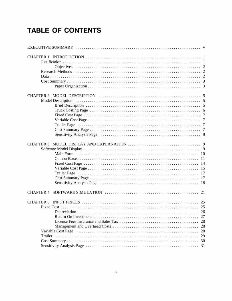
TABLE OF CONTENTS

EXECUTIVE SUMMARY . . . . . . . . . . . . . . . . . . . . . . . . . . . . . . . . . . . . . . . . . . . . . . . . . . . . . . . . . . . . v

CHAPTER 1. INTRODUCTION . . . . . . . . . . . . . . . . . . . . . . . . . . . . . . . . . . . . . . . . . . . . . . . . . . . . . . . 1Justification . . . . . . . . . . . . . . . . . . . . . . . . . . . . . . . . . . . . . . . . . . . . . . . . . . . . . . . . . . . . . . . . . . 1

Objectives . . . . . . . . . . . . . . . . . . . . . . . . . . . . . . . . . . . . . . . . . . . . . . . . . . . . . . . . . . . . 2Research Methods . . . . . . . . . . . . . . . . . . . . . . . . . . . . . . . . . . . . . . . . . . . . . . . . . . . . . . . . . . . . . 2Data . . . . . . . . . . . . . . . . . . . . . . . . . . . . . . . . . . . . . . . . . . . . . . . . . . . . . . . . . . . . . . . . . . . . . . . . 2Cost Summary . . . . . . . . . . . . . . . . . . . . . . . . . . . . . . . . . . . . . . . . . . . . . . . . . . . . . . . . . . . . . . . . 3

Paper Organization . . . . . . . . . . . . . . . . . . . . . . . . . . . . . . . . . . . . . . . . . . . . . . . . . . . . . . 3

CHAPTER 2. MODEL DESCRIPTION . . . . . . . . . . . . . . . . . . . . . . . . . . . . . . . . . . . . . . . . . . . . . . . . . 5Model Description . . . . . . . . . . . . . . . . . . . . . . . . . . . . . . . . . . . . . . . . . . . . . . . . . . . . . . . . . . . . 5

Brief Description . . . . . . . . . . . . . . . . . . . . . . . . . . . . . . . . . . . . . . . . . . . . . . . . . . . . . . . 5Truck Costing Page . . . . . . . . . . . . . . . . . . . . . . . . . . . . . . . . . . . . . . . . . . . . . . . . . . . . . 6Fixed Cost Page . . . . . . . . . . . . . . . . . . . . . . . . . . . . . . . . . . . . . . . . . . . . . . . . . . . . . . . . 7

Variable Cost Page . . . . . . . . . . . . . . . . . . . . . . . . . . . . . . . . . . . . . . . . . . . . . . . . . . . . . . 7Trailer Page . . . . . . . . . . . . . . . . . . . . . . . . . . . . . . . . . . . . . . . . . . . . . . . . . . . . . . . . . . . 7Cost Summary Page . . . . . . . . . . . . . . . . . . . . . . . . . . . . . . . . . . . . . . . . . . . . . . . . . . . . . 7Sensitivity Analysis Page . . . . . . . . . . . . . . . . . . . . . . . . . . . . . . . . . . . . . . . . . . . . . . . . . 8

CHAPTER 3. MODEL DISPLAY AND EXPLANATION . . . . . . . . . . . . . . . . . . . . . . . . . . . . . . . . . . . 9Software Model Display . . . . . . . . . . . . . . . . . . . . . . . . . . . . . . . . . . . . . . . . . . . . . . . . . . . . . . . . 9

Main Form . . . . . . . . . . . . . . . . . . . . . . . . . . . . . . . . . . . . . . . . . . . . . . . . . . . . . . . . . . . 10Combo Boxes . . . . . . . . . . . . . . . . . . . . . . . . . . . . . . . . . . . . . . . . . . . . . . . . . . . . . . . . . 11Fixed Cost Page . . . . . . . . . . . . . . . . . . . . . . . . . . . . . . . . . . . . . . . . . . . . . . . . . . . . . . . 14Variable Cost Page . . . . . . . . . . . . . . . . . . . . . . . . . . . . . . . . . . . . . . . . . . . . . . . . . . . . . 15Trailer Page . . . . . . . . . . . . . . . . . . . . . . . . . . . . . . . . . . . . . . . . . . . . . . . . . . . . . . . . . . 17Cost Summary Page . . . . . . . . . . . . . . . . . . . . . . . . . . . . . . . . . . . . . . . . . . . . . . . . . . . . 17

Sensitivity Analysis Page . . . . . . . . . . . . . . . . . . . . . . . . . . . . . . . . . . . . . . . . . . . . . . . . 18

CHAPTER 4. SOFTWARE SIMULATION . . . . . . . . . . . . . . . . . . . . . . . . . . . . . . . . . . . . . . . . . . . . . 21

CHAPTER 5. INPUT PRICES . . . . . . . . . . . . . . . . . . . . . . . . . . . . . . . . . . . . . . . . . . . . . . . . . . . . . . . . 25Fixed Cost . . . . . . . . . . . . . . . . . . . . . . . . . . . . . . . . . . . . . . . . . . . . . . . . . . . . . . . . . . . . . . . . . . 25

Depreciation . . . . . . . . . . . . . . . . . . . . . . . . . . . . . . . . . . . . . . . . . . . . . . . . . . . . . . . . . . 26Return On Investment . . . . . . . . . . . . . . . . . . . . . . . . . . . . . . . . . . . . . . . . . . . . . . . . . . 27License Fees Insurance and Sales Tax . . . . . . . . . . . . . . . . . . . . . . . . . . . . . . . . . . . . . . 28Management and Overhead Costs . . . . . . . . . . . . . . . . . . . . . . . . . . . . . . . . . . . . . . . . . 28

Variable Cost Page . . . . . . . . . . . . . . . . . . . . . . . . . . . . . . . . . . . . . . . . . . . . . . . . . . . . . . . . . . . 28Trailer . . . . . . . . . . . . . . . . . . . . . . . . . . . . . . . . . . . . . . . . . . . . . . . . . . . . . . . . . . . . . . . . . . . . . 29Cost Summary . . . . . . . . . . . . . . . . . . . . . . . . . . . . . . . . . . . . . . . . . . . . . . . . . . . . . . . . . . . . . . . 30Sensitivity Analysis Page . . . . . . . . . . . . . . . . . . . . . . . . . . . . . . . . . . . . . . . . . . . . . . . . . . . . . . 31

ii

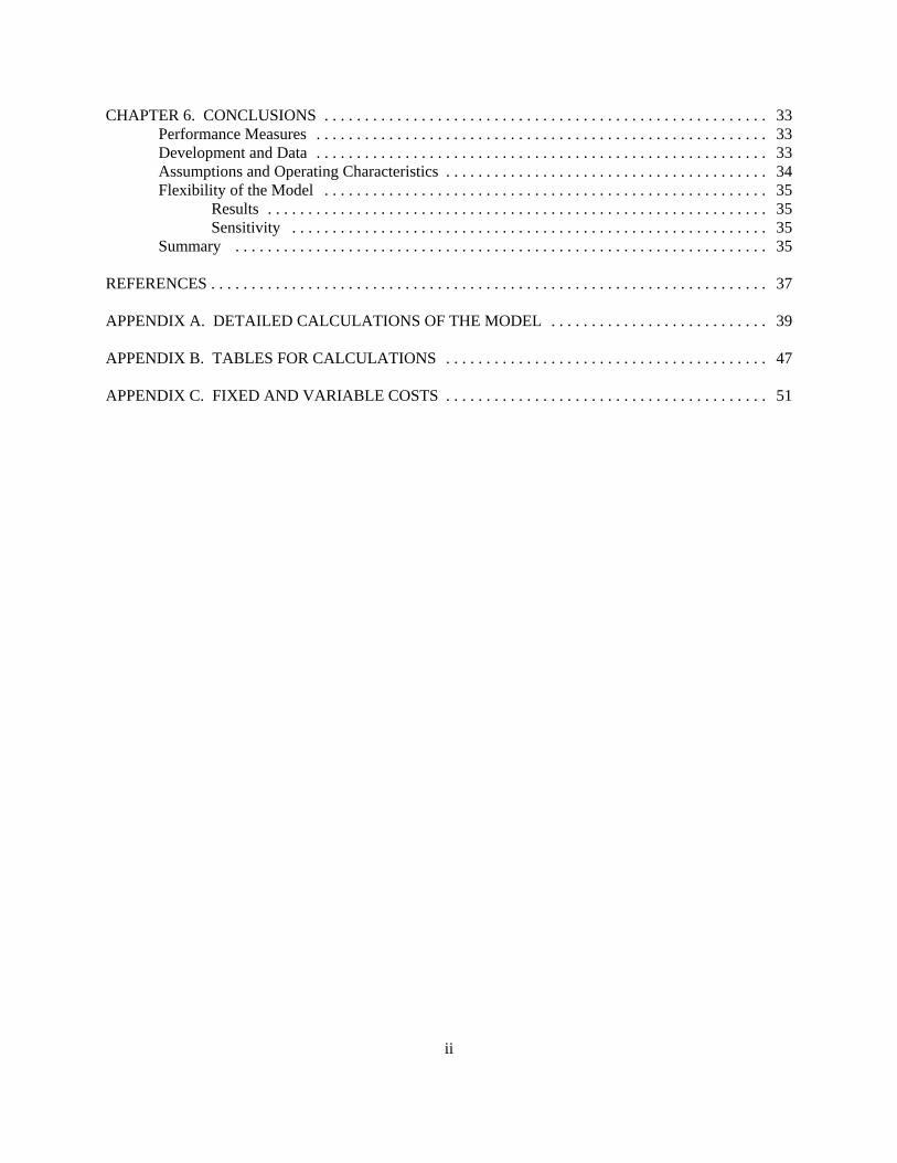
CHAPTER 6. CONCLUSIONS . . . . . . . . . . . . . . . . . . . . . . . . . . . . . . . . . . . . . . . . . . . . . . . . . . . . . . . 33Performance Measures . . . . . . . . . . . . . . . . . . . . . . . . . . . . . . . . . . . . . . . . . . . . . . . . . . . . . . . . 33Development and Data . . . . . . . . . . . . . . . . . . . . . . . . . . . . . . . . . . . . . . . . . . . . . . . . . . . . . . . . 33Assumptions and Operating Characteristics . . . . . . . . . . . . . . . . . . . . . . . . . . . . . . . . . . . . . . . . 34Flexibility of the Model . . . . . . . . . . . . . . . . . . . . . . . . . . . . . . . . . . . . . . . . . . . . . . . . . . . . . . . 35

Results . . . . . . . . . . . . . . . . . . . . . . . . . . . . . . . . . . . . . . . . . . . . . . . . . . . . . . . . . . . . . . 35Sensitivity . . . . . . . . . . . . . . . . . . . . . . . . . . . . . . . . . . . . . . . . . . . . . . . . . . . . . . . . . . . 35

Summary . . . . . . . . . . . . . . . . . . . . . . . . . . . . . . . . . . . . . . . . . . . . . . . . . . . . . . . . . . . . . . . . . . 35

REFERENCES . . . . . . . . . . . . . . . . . . . . . . . . . . . . . . . . . . . . . . . . . . . . . . . . . . . . . . . . . . . . . . . . . . . . . 37

APPENDIX A. DETAILED CALCULATIONS OF THE MODEL . . . . . . . . . . . . . . . . . . . . . . . . . . . 39

APPENDIX B. TABLES FOR CALCULATIONS . . . . . . . . . . . . . . . . . . . . . . . . . . . . . . . . . . . . . . . . 47

APPENDIX C. FIXED AND VARIABLE COSTS . . . . . . . . . . . . . . . . . . . . . . . . . . . . . . . . . . . . . . . . 51

iii

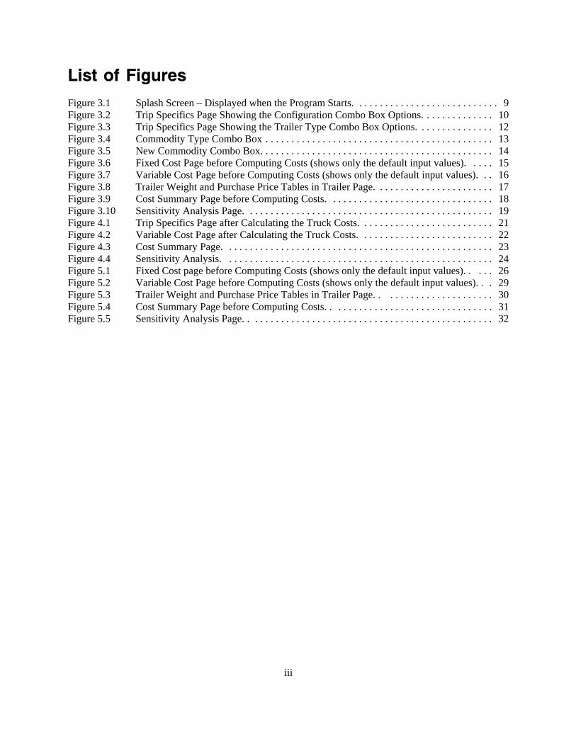
List of Figures

Figure 3.1 Splash Screen – Displayed when the Program Starts. . . . . . . . . . . . . . . . . . . . . . . . . . . . 9Figure 3.2 Trip Specifics Page Showing the Configuration Combo Box Options. . . . . . . . . . . . . . 10Figure 3.3 Trip Specifics Page Showing the Trailer Type Combo Box Options. . . . . . . . . . . . . . . 12Figure 3.4 Commodity Type Combo Box . . . . . . . . . . . . . . . . . . . . . . . . . . . . . . . . . . . . . . . . . . . . 13Figure 3.5 New Commodity Combo Box. . . . . . . . . . . . . . . . . . . . . . . . . . . . . . . . . . . . . . . . . . . . . 14Figure 3.6 Fixed Cost Page before Computing Costs (shows only the default input values). . . . . 15Figure 3.7 Variable Cost Page before Computing Costs (shows only the default input values). . . 16Figure 3.8 Trailer Weight and Purchase Price Tables in Trailer Page. . . . . . . . . . . . . . . . . . . . . . . 17Figure 3.9 Cost Summary Page before Computing Costs. . . . . . . . . . . . . . . . . . . . . . . . . . . . . . . . 18Figure 3.10 Sensitivity Analysis Page. . . . . . . . . . . . . . . . . . . . . . . . . . . . . . . . . . . . . . . . . . . . . . . . 19Figure 4.1 Trip Specifics Page after Calculating the Truck Costs. . . . . . . . . . . . . . . . . . . . . . . . . . 21Figure 4.2 Variable Cost Page after Calculating the Truck Costs. . . . . . . . . . . . . . . . . . . . . . . . . . 22Figure 4.3 Cost Summary Page. . . . . . . . . . . . . . . . . . . . . . . . . . . . . . . . . . . . . . . . . . . . . . . . . . . . 23Figure 4.4 Sensitivity Analysis. . . . . . . . . . . . . . . . . . . . . . . . . . . . . . . . . . . . . . . . . . . . . . . . . . . . 24Figure 5.1 Fixed Cost page before Computing Costs (shows only the default input values). . . . . 26Figure 5.2 Variable Cost Page before Computing Costs (shows only the default input values). . . 29Figure 5.3 Trailer Weight and Purchase Price Tables in Trailer Page. . . . . . . . . . . . . . . . . . . . . . 30Figure 5.4 Cost Summary Page before Computing Costs. . . . . . . . . . . . . . . . . . . . . . . . . . . . . . . . 31Figure 5.5 Sensitivity Analysis Page. . . . . . . . . . . . . . . . . . . . . . . . . . . . . . . . . . . . . . . . . . . . . . . . 32

iv

v

EXECUTIVE SUMMARY

Truckers face different input prices, product characteristics, truck configurations, geographical characteristics,firm size, and driving practices. Thus, it is difficult to obtain current estimates of costs for particularindependent owner/operators. The software that was developed determines costs for a variety of truckconfigurations, product characteristics, and input prices. A firm's costs are determined by its equipment,characteristics of products hauled, and input prices associated with a typical movement for that firm.

The truck costing software may provide information to many in the trucking and or shipping industry.Anyone estimating transportation costs need reliable estimates of owner/operator costs. Also some shippersneed accurate truck cost information to negotiate desirable rates and determine the appropriate mode oftransportation.

A stand alone Truck Costing Model was developed using Microsoft Visual Basic for Windows. The modelin this study has many useful features. Costs can be obtained for many different configurations and tripcharacteristics. Important conclusions can be drawn from running simulations include the sensitivity of costsand equipment use, wait time and trip distance, labor, and fuel price. The relationships of these variables andthe cost of operations are important for trucking interests.

The simulations and sensitivity analysis determined the truck cost model's flexibility and inadequacies.Factors influencing costs of owner/operators include annual miles, trip distance, and truck speed for fuelefficiency. Decreasing annual miles may be critical for the trucker debating on waiting for a better revenueload. The opportunity cost of waiting may more than make up for the additional revenue received. Anotherinteresting factor in the model is the wait time. Initial assumptions exclude wait time, but loading andunloading time for short movements are the driving force of increased costs. The shorter the trip, the greaterthe impact of loading and unloading time on cost.

vi

1

CHAPTER 1. INTRODUCTION

The motor carrier industry has been a recurrent subject for cost studies. Most referenced studies use aneconomic-engineering approach to estimate trucking costs. The economic-engineering model estimates theproduction function with a given set of factor prices. Some studies use surveys as a data collecting tool toarrive at costs by averaging information received from the survey. Cost components are easily identified inthe economic-engineering approach and thus, cost estimates of a new startup firm are readily available. Aweakness of the economic-engineering approach is that results are based on average values of input pricesand resource usage, and are accurate for a limited population. Furthermore, a new study must be undertakento update the results.

This model aims to provide for adaptability for the different users. The focus is on individual motor carriercosting for a single movement.

Justification

An Owner/Operator Spreadsheet Costing Model developed in 1996 has been useful. However, it is based ona spreadsheet and lacked functionality of a stand alone model or software product. A new visual basic modelhas been developed to be a stand alone product that may be employed by transportation professionals andresearchers. The model can be expanded to include many truck configurations.

Although the trucking industry is perceived as a competitive homogenous industry, many characteristicssegment the industry into subindustries. The trucking industry is classified as either local or intercity. Vastdifferences exist between these two segments. Local carriers include intracity services such as delivery, dumptrucks, garbage trucks, and other services (Titus, 1994). Intercity trucking is classified between less-than-truckload (trucks hauling less than 10,000 pounds) and the truckload sectors. The focus of the softwareproduct is on the intercity truckload sector and, more specifically, a specific movement of a single tractortrailer unit.

Many small truckload (TL) firms operate in the motor carrier industry. An estimated 575,000 truckingcompanies operate in the United States (Federal Motor Carrier Administration, 2002). It is estimated thatmore than 95 percent of trucking companies have less than $1 million in gross revenue (Coyle, Bardi, andNovak, 1994). Many of these smaller companies are owner/operators or small firms with a single unit or onlya few trucks.

Truckers face different input prices, product characteristics, truck configurations, geographical characteristics,firm size, and driving practices. Thus, obtaining current estimates of costs for particular independentowner/operators is difficult. The software that was developed determines costs for a variety of truckconfigurations, product characteristics, and input prices. A firm's costs are determined by its equipment,characteristics of products hauled, and input prices associated with a typical movement for that firm.

The truck costing software may provide information to many in the trucking and or shipping industry.Anyone estimating transportation costs need reliable estimates of owner/operator costs. Also some shippersneed accurate truck cost information to negotiate desirable rates and determine the appropriate mode oftransportation.

1A performance measure in the trucking industry is the unit cost such as per-mile, per-ton, per hour etc.

2

Owner/operator cost information helps larger trucking firms that use owner/operators. Owner/operators lease(enter into contract) to a larger firm and current cost estimates may be beneficial to both parties in negotiatingthe agreement.

The trucking industry is not homogenous; but, the industry approximates perfect competition because it haslimited entry barriers, a large number of firms, virtually perfect information, and its small independenttruckers mainly are price takers. There are many entries and exits from the industry annually. For firmsneeding the owner/operator services, sustainability may reduce search costs and improve transportationservice through reduced turnover.

Current transportation cost estimates are essential for economic development or those providing feasibilityof possible manufacturing or other facilities. Current cost information again may allow intermodaltransportation rate comparisons and provide transportation information vital to the location of a new facility.

Objectives

The primary objective of this project was to develop a software model that provides truck cost informationreflecting differences in equipment, product, and trip characteristics of an individual firm. A secondaryobjective was to provide additional performance measures for decision makers who use truck costinformation1. The different performance measures generated can be used by different entities for specificpurposes.

Research Methods

Developing costs in the trucking industry requires use of many data sources. Secondary data sources includedata for equipment, trip, and industry characteristics. A literature review was conducted to identify data fromprior truck costing studies and to evaluate past methods to form assumptions and determine relevant costs forthe industry. Interviews were conducted with various trucking experts to gather data related to trucking costs.A Microsoft Visual Basic model was developed to link relevant truck costs to performance measures. Ahighlight of the model is that sensitivity analysis can be conducted to determine the model’s sensitivity tochanging input variables. The model’s design enables a user to change most parameters to fit individualneeds.

Data

Data used to build the original truck cost spreadsheet model came from a variety of sources includinginterview and secondary data sources. Some data and formulas used in the original spreadsheet model havebeen updated and verified for reliability. The new software model also allows the user to change data thatdoes not reflect a particular input, equipment cost, or trip characteristic.

3

Cost Summary

Factors affecting costs in the trucking industry include economies of size, economies of utilization, and themakeup of variable and fixed costs. Economies of size for small firms and owner/operators are minimal, andthe cost structure of owner/operators vary from larger firms because management and overhead costs maybe low or negligible. For small firms or owner/operators, increasing company size by adding power unitsmay result in volume discounts for purchasing larger quantities of inputs.

Utilization of equipment is the most important factor affecting motor carriers. High use of equipment lowersaverage fixed costs. It would be expected that small changes in equipment use may have a large impact oncosts for the owner/operator.

Paper Organization

This paper is divided into five parts. Industry cost structure and the literature are examined. Modeldevelopment is explained. Model results and sensitivity analysis are presented and a conclusion andsummary.

4

5

CHAPTER 2. MODEL DESCRIPTION

Bierman, Bonini, and Hausman (1991) describe a model as a "simplified representation of an empiricalsituation." This software model attempts to replicate the actual movement of a product by a motor carrier.Variables are classified as decision variables, exogenous variables, intermediate variables, policies andconstraints, or performance measures. Decision variables are under the control of the decision maker. Theother types of variables affect the model, but their values cannot be determined by the decision maker.

Exogenous or external variables are outside the decision maker's control. Intermediate variables are used torelate decision variables and exogenous variables to performance measures (Bierman, et al., 1991).Exogenous and intermediate variables are represented in various places throughout the model.

Truck costs are a function of decisions made by a company or owner/operator. The differences in equipmentcharacteristics, and operational structure, along with different trip characteristics, result in a somewhat uniquecost structure for a particular movement and/or firm. Firm costs such as fuel, insurance, labor, maintenanceand repair costs vary depending on geography, new versus used, and freight being transported. The modelallows decision makers to change parameters to reflect different decisions which impact transportation cost.

The software model can calculate truck cost for many commodities using different truck equipmentcombinations and input prices. This application provides per mile, per hour, per bushel, per hundredweight,per ton, per gallon, and the option of a user defined unit cost or performance measure for a particular trip.

The following sections describe features of the model and provide examples for use. Formulas and other dataalso are displayed.

Model Description

The software interface must have parameter entries and definitions prior to trip simulations being computed.The program can be run repeatedly, allowing for different inputs simulating different input parameters. Thesensitivity analysis feature of the model allows the user to see how sensitive the model is to changing inputprices and how those changes reflect cost. The model was constructed using Visual Basic programminglanguage. Visual Basic allows a programmer to develop applications with graphical user interfaces that runin Microsoft’s Windows without the complexity generally associated with Windows programming.

This application includes three forms: a splash screen form, a main form, and a small pop up form used toadd new commodity type or unit. The next section provides a brief description of the model and thendescribes the different pages in depth with a visual display.

Brief Description

The operator of the software defines the firm’s operating and trip characteristics. The model calculates costsbased on those decisions and there are many options available. The model is unique, as it can be run for manydifferent options, and the options may be compared to determine a low cost solution. This section firstexplains the contents of the different pages. Next, it describes calculations the model performs, and last itdiscusses the performance measures or output of the model.

2Rocky Mountain Double is a six-axle semi truck pulling a two-axle trailer. Conventional is a five-axlesemi (most common), a spread tandem is a five-axle semi where the trailer axles are set apart to take advantage ofweight restrictions. A tridem is a six-axle semi.

6

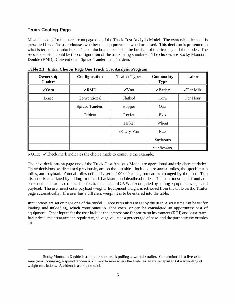
Truck Costing Page

Most decisions for the user are on page one of the Truck Cost Analysis Model. The ownership decision ispresented first. The user chooses whether the equipment is owned or leased. This decision is presented inwhat is termed a combo box. The combo box is located at the far right of the first page of the model. Thesecond decision could be the configuration of the truck being simulated. The choices are Rocky MountainDouble (RMD), Conventional, Spread Tandem, and Tridem.2

Table 2.1. Initial Choices Page One Truck Cost Analysis Program

OwnershipChoices

Configuration Trailer Types CommodityType

Labor

TOwn TRMD TVan TBarley TPer Mile

Lease Conventional Flatbed Corn Per Hour

Spread Tandem Hopper Oats

Tridem Reefer Flax

Tanker Wheat

53' Dry Van Flax

Soybeans

SunflowersNOTE: TCheck mark indicates the choice made to compute the example.

The next decisions on page one of the Truck Cost Analysis Model are operational and trip characteristics.These decisions, as discussed previously, are on the left side. Included are annual miles, the specific tripmiles, and payload. Annual miles default is set at 100,000 miles, but can be changed by the user. Tripdistance is calculated by adding fronthaul, backhaul, and deadhead miles. The user must enter fronthaul,backhaul and deadhead miles. Tractor, trailer, and total GVW are computed by adding equipment weight andpayload. The user must enter payload weight. Equipment weight is retrieved from the table on the Trailerpage automatically. If a user has a different weight it is to be entered into the table.

Input prices are set on page one of the model. Labor rates also are set by the user. A wait time can be set forloading and unloading, which contributes to labor costs, or can be considered an opportunity cost ofequipment. Other inputs for the user include the interest rate for return on investment (ROI) and lease rates,fuel prices, maintenance and repair rate, salvage value as a percentage of new, and the purchase tax or salestax.

7

Fixed Cost Page

The Fixed Cost page includes computed values and others that can be changed. On this page the tractor pricecan be changed and the estimated useful life for the tractor and the trailer can be varied to reflect differentequipment usage affecting annual equipment price. In the equipment ownership and lease expense sectionscosts are displayed along with depreciation and ROI.

Also on the Fixed Cost page are the license, taxes, and insurance entries with defaults set. Computed in thetable is the annual fixed costs, which are converted to the different performance measures.

Variable Cost Page

The Variable Cost Page contains five sections. The sections are tire, fuel, maintenance and repair, labor, andtotal variable costs. In the tire section is the cost per tire separated by tractor tires and trailer tires. There iscost per mile loaded and empty for both tractor and trailer. There also is calculated cells for weight per tireand costs per mile per tire.

The fuel costs have cells for calculations on miles per gallon empty and loaded, and adjusted for speed. Thefinal cells in the table are fuel cost per mile loaded and empty.

The maintenance and repair section shows the calculated values for loaded and empty. This section iscalculated by the model and those calculations are explained later.

The labor cells show the labor cost per mile, from driving and waiting. These entries are calculated fromdecisions made on page one of the model.

Trailer Page

The Trailer page contains two tables. The first table has the trailer weights. These are used throughout todetermine GVW, tire numbers, and other calculations. These can be changed before the model is run forspecific trailer weights for different equipment to provide a more accurate cost estimate.

The second table is the trailer prices. These are default prices established from industry experts. These pricescan be changed before the model is run for specific equipment providing a more accurate cost estimate.

Cost Summary Page

The Cost Summary page contains the performance measures or the output of the software model. Themeasures are separated into fixed and variable costs and also into different costing units or performancemeasurements. Variable costs are fuel, labor, tires, and maintenance and repair. Fixed costs are equipmentcosts, license and taxes, insurance, and management and overhead.

As stated earlier, these costs are measured using several different performance measures. These measuresare per mile, per hour, per bushel, per hundredweight, per ton, per trip, per gallon or other unit that can bedesignated by the user at the outset of running the model.

8

Sensitivity Analysis Page

The Sensitivity Analysis page contains many variables that can be changed to see the model's reaction orsensitivity to these variables. The variables can be chosen independently and positive and negativepercentages can be used to test sensitivity. The change in costs are presented as percentage effects on originalcosts. This provides the user with flexibility in testing variables’ influences on truck costs.

9

Figure 3.1. Splash Screen – Displayed when theProgram Starts

CHAPTER 3. MODEL DISPLAY AND EXPLANATION

This chapter will show different displays of the model and explain how entries may be changed. The goalis to provide a user with an understanding of how to use the model. As stated earlier, the model is made upof different pages that are accessed by using “SSTabs.” The following description and figures explains andshows how to use the model.

Software Model Display

The truck cost software application splash screen is displayed as the application loads. An example of thesplash screen is shown as Figure 3.1.

10

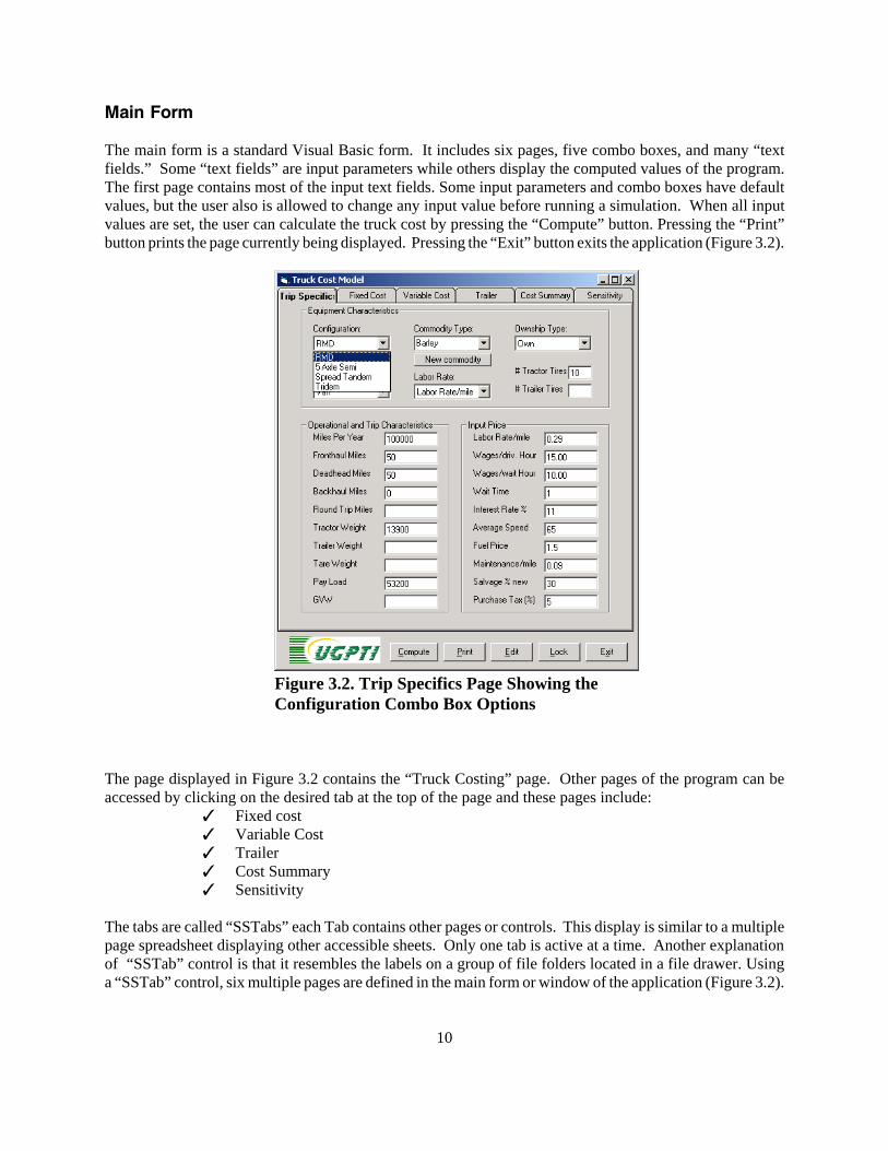
Figure 3.2. Trip Specifics Page Showing theConfiguration Combo Box Options

Main Form

The main form is a standard Visual Basic form. It includes six pages, five combo boxes, and many “textfields.” Some “text fields” are input parameters while others display the computed values of the program.The first page contains most of the input text fields. Some input parameters and combo boxes have defaultvalues, but the user also is allowed to change any input value before running a simulation. When all inputvalues are set, the user can calculate the truck cost by pressing the “Compute” button. Pressing the “Print”button prints the page currently being displayed. Pressing the “Exit” button exits the application (Figure 3.2).

The page displayed in Figure 3.2 contains the “Truck Costing” page. Other pages of the program can beaccessed by clicking on the desired tab at the top of the page and these pages include:

T Fixed costT Variable CostT TrailerT Cost SummaryT Sensitivity

The tabs are called “SSTabs” each Tab contains other pages or controls. This display is similar to a multiplepage spreadsheet displaying other accessible sheets. Only one tab is active at a time. Another explanationof “SSTab” control is that it resembles the labels on a group of file folders located in a file drawer. Usinga “SSTab” control, six multiple pages are defined in the main form or window of the application (Figure 3.2).

3Bridge formulas are created to determine the maximum gross weight allowable on the structure and stillmeet strict safety requirements. North Dakota highways and interstates use Bridge Formula B to determine theallowable gross weight on bridges. State highways and Interstates use the same bridge formula. Current bridgeformulas allow extra weight for longer vehicles and for vehicles with more axles. Longer vehicles reduce bridgestress and more axles on a vehicle reduces its impact on pavement (LeAnn Emmer, interview, July, 2000).

11

Users can navigate between pages either by pressing “CTRL+TAB” on the keyboard, or by clicking the leftmouse button on the caption of each tab.

Combo Boxes

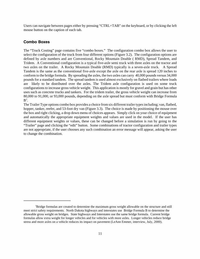
The “Truck Costing” page contains five “combo boxes.” The configuration combo box allows the user toselect the configuration of the truck from four different options (Figure 3.2). The configuration options aredefined by axle numbers and are Conventional, Rocky Mountain Double ( RMD), Spread Tandem, andTridem. A Conventional configuration is a typical five-axle semi truck with three axles on the tractor andtwo axles on the trailer. A Rocky Mountain Double (RMD) typically is a seven-axle truck. A SpreadTandem is the same as the conventional five-axle except the axle on the rear axle is spread 120 inches toconform to the bridge formula. By spreading the axles, the two axles can carry 40,000 pounds versus 34,000pounds for a standard tandem. The spread tandem is used almost exclusively on flatbed trailers where loadsare likely to be distributed over the axles. The Tridem axle configuration is used on some truckconfigurations to increase gross vehicle weight. This application is mostly for gravel and grain but has otheruses such as concrete trucks and tankers. For the tridem trailer, the gross vehicle weight can increase from80,000 to 91,000, or 93,000 pounds, depending on the axle spread but must conform with Bridge FormulaB3. The Trailer Type options combo box provides a choice from six different trailer types including; van, flatbed,hopper, tanker, reefer, and 53-foot dry van (Figure 3.3). The choice is made by positioning the mouse overthe box and right clicking, a drop down menu of choices appears. Simply click on your choice of equipmentand automatically the appropriate equipment weights and values are used in the model. If the user hasdifferent equipment weights or values, these can be changed before a simulation is run by going to the“Trailer” page and clicking the “edit” button. Some combinations of tractor configuration and trailer typesare not appropriate, if the user chooses any such combination an error message will appear, asking the userto change the combination.

12

Figure 3.3. Trip Specifics Page Showing the TrailerType Combo Box Options

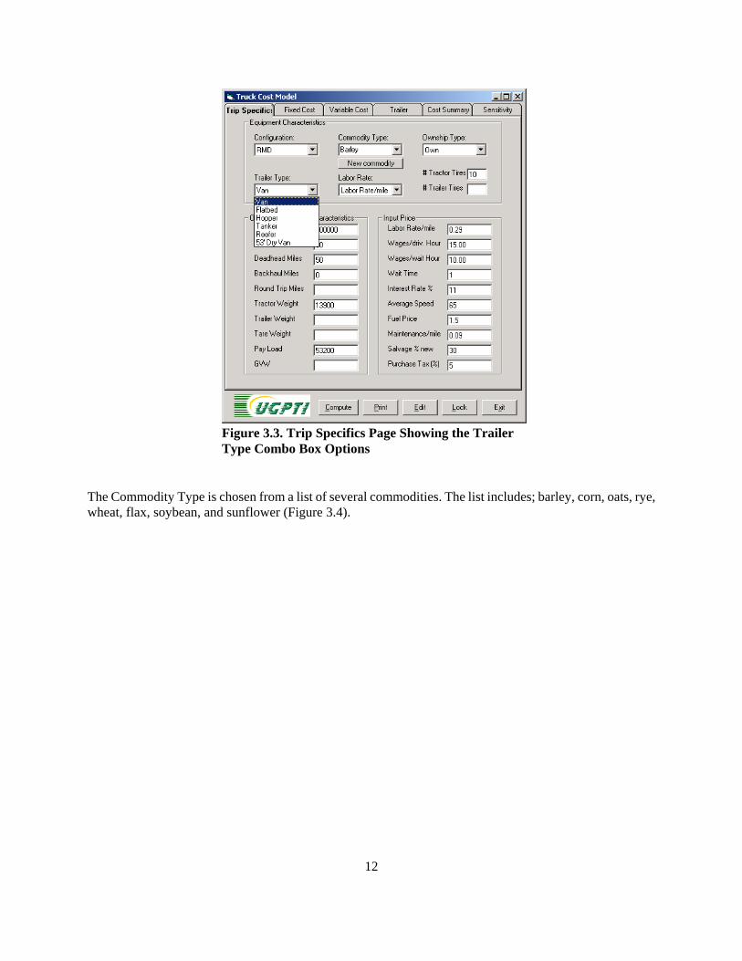
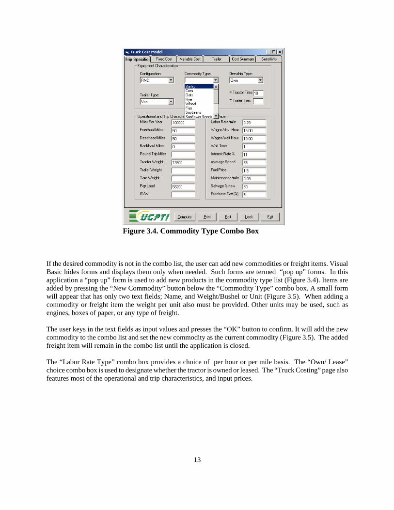
The Commodity Type is chosen from a list of several commodities. The list includes; barley, corn, oats, rye,wheat, flax, soybean, and sunflower (Figure 3.4).

13

Figure 3.4. Commodity Type Combo Box

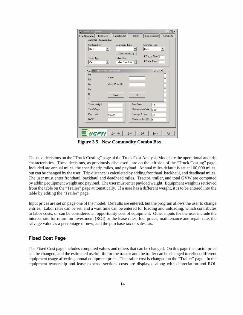
If the desired commodity is not in the combo list, the user can add new commodities or freight items. VisualBasic hides forms and displays them only when needed. Such forms are termed “pop up” forms. In thisapplication a “pop up” form is used to add new products in the commodity type list (Figure 3.4). Items areadded by pressing the “New Commodity” button below the “Commodity Type” combo box. A small formwill appear that has only two text fields; Name, and Weight/Bushel or Unit (Figure 3.5). When adding acommodity or freight item the weight per unit also must be provided. Other units may be used, such asengines, boxes of paper, or any type of freight.

The user keys in the text fields as input values and presses the “OK” button to confirm. It will add the newcommodity to the combo list and set the new commodity as the current commodity (Figure 3.5). The addedfreight item will remain in the combo list until the application is closed.

The “Labor Rate Type” combo box provides a choice of per hour or per mile basis. The “Own/ Lease”choice combo box is used to designate whether the tractor is owned or leased. The “Truck Costing” page alsofeatures most of the operational and trip characteristics, and input prices.

14

Figure 3.5. New Commodity Combo Box.

The next decisions on the “Truck Costing” page of the Truck Cost Analysis Model are the operational and tripcharacteristics. These decisions, as previously discussed , are on the left side of the “Truck Costing” page.Included are annual miles, the specific trip miles, and payload. Annual miles default is set at 100,000 miles,but can be changed by the user. Trip distance is calculated by adding fronthaul, backhaul, and deadhead miles.The user must enter fronthaul, backhaul and deadhead miles. Tractor, trailer, and total GVW are computedby adding equipment weight and payload. The user must enter payload weight. Equipment weight is retrievedfrom the table on the “Trailer” page automatically. If a user has a different weight, it is to be entered into thetable by editing the “Trailer” page.

Input prices are set on page one of the model. Defaults are entered, but the program allows the user to changeentries. Labor rates can be set, and a wait time can be entered for loading and unloading, which contributesto labor costs, or can be considered an opportunity cost of equipment. Other inputs for the user include theinterest rate for return on investment (ROI) or the lease rates, fuel prices, maintenance and repair rate, thesalvage value as a percentage of new, and the purchase tax or sales tax.

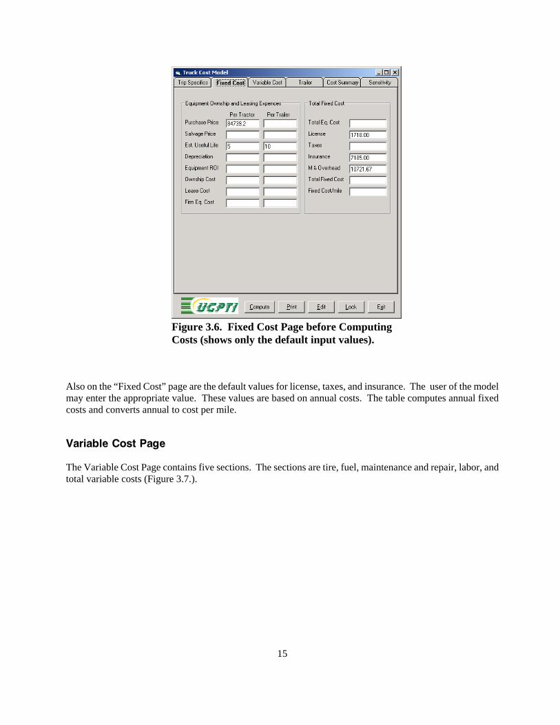
Fixed Cost Page

The Fixed Cost page includes computed values and others that can be changed. On this page the tractor pricecan be changed, and the estimated useful life for the tractor and the trailer can be changed to reflect differentequipment usage affecting annual equipment price. The trailer cost is changed on the “Trailer” page. In theequipment ownership and lease expense sections costs are displayed along with depreciation and ROI.

15

Figure 3.6. Fixed Cost Page before ComputingCosts (shows only the default input values).

Also on the “Fixed Cost” page are the default values for license, taxes, and insurance. The user of the modelmay enter the appropriate value. These values are based on annual costs. The table computes annual fixedcosts and converts annual to cost per mile.

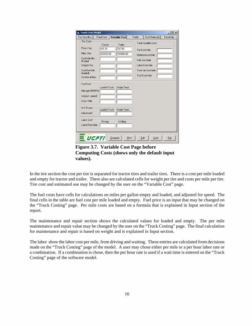
Variable Cost Page

The Variable Cost Page contains five sections. The sections are tire, fuel, maintenance and repair, labor, andtotal variable costs (Figure 3.7.).

16

Figure 3.7. Variable Cost Page beforeComputing Costs (shows only the default inputvalues).

In the tire section the cost per tire is separated for tractor tires and trailer tires. There is a cost per mile loadedand empty for tractor and trailer. There also are calculated cells for weight per tire and costs per mile per tire.Tire cost and estimated use may be changed by the user on the “Variable Cost” page.

The fuel costs have cells for calculations on miles per gallon empty and loaded, and adjusted for speed. Thefinal cells in the table are fuel cost per mile loaded and empty. Fuel price is an input that may be changed onthe “Truck Costing” page. Per mile costs are based on a formula that is explained in Input section of thereport.

The maintenance and repair section shows the calculated values for loaded and empty. The per milemaintenance and repair value may be changed by the user on the “Truck Costing” page. The final calculationfor maintenance and repair is based on weight and is explained in Input section.

The labor show the labor cost per mile, from driving and waiting. These entries are calculated from decisionsmade on the “Truck Costing” page of the model. A user may chose either per mile or a per hour labor rate ora combination. If a combination is chose, then the per hour rate is used if a wait time is entered on the “TruckCosting” page of the software model.

17

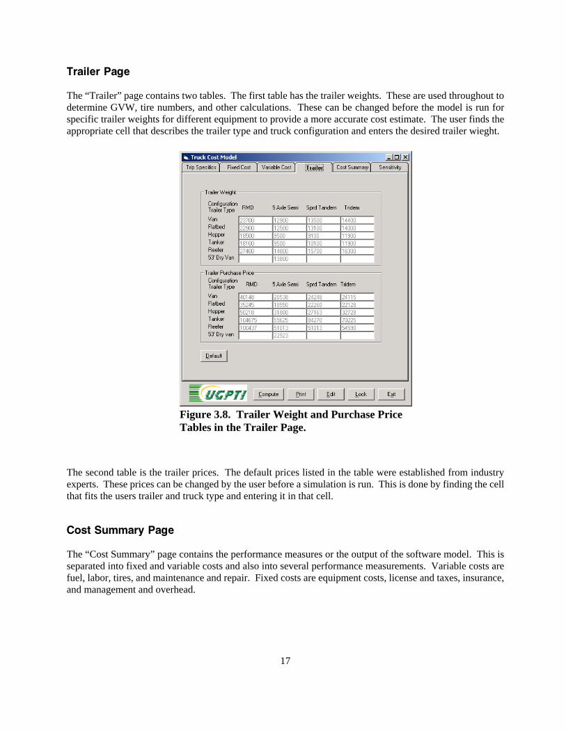
Figure 3.8. Trailer Weight and Purchase PriceTables in the Trailer Page.

Trailer Page

The “Trailer” page contains two tables. The first table has the trailer weights. These are used throughout todetermine GVW, tire numbers, and other calculations. These can be changed before the model is run forspecific trailer weights for different equipment to provide a more accurate cost estimate. The user finds theappropriate cell that describes the trailer type and truck configuration and enters the desired trailer wieght.

The second table is the trailer prices. The default prices listed in the table were established from industryexperts. These prices can be changed by the user before a simulation is run. This is done by finding the cellthat fits the users trailer and truck type and entering it in that cell.

Cost Summary Page

The “Cost Summary” page contains the performance measures or the output of the software model. This isseparated into fixed and variable costs and also into several performance measurements. Variable costs arefuel, labor, tires, and maintenance and repair. Fixed costs are equipment costs, license and taxes, insurance,and management and overhead.

18

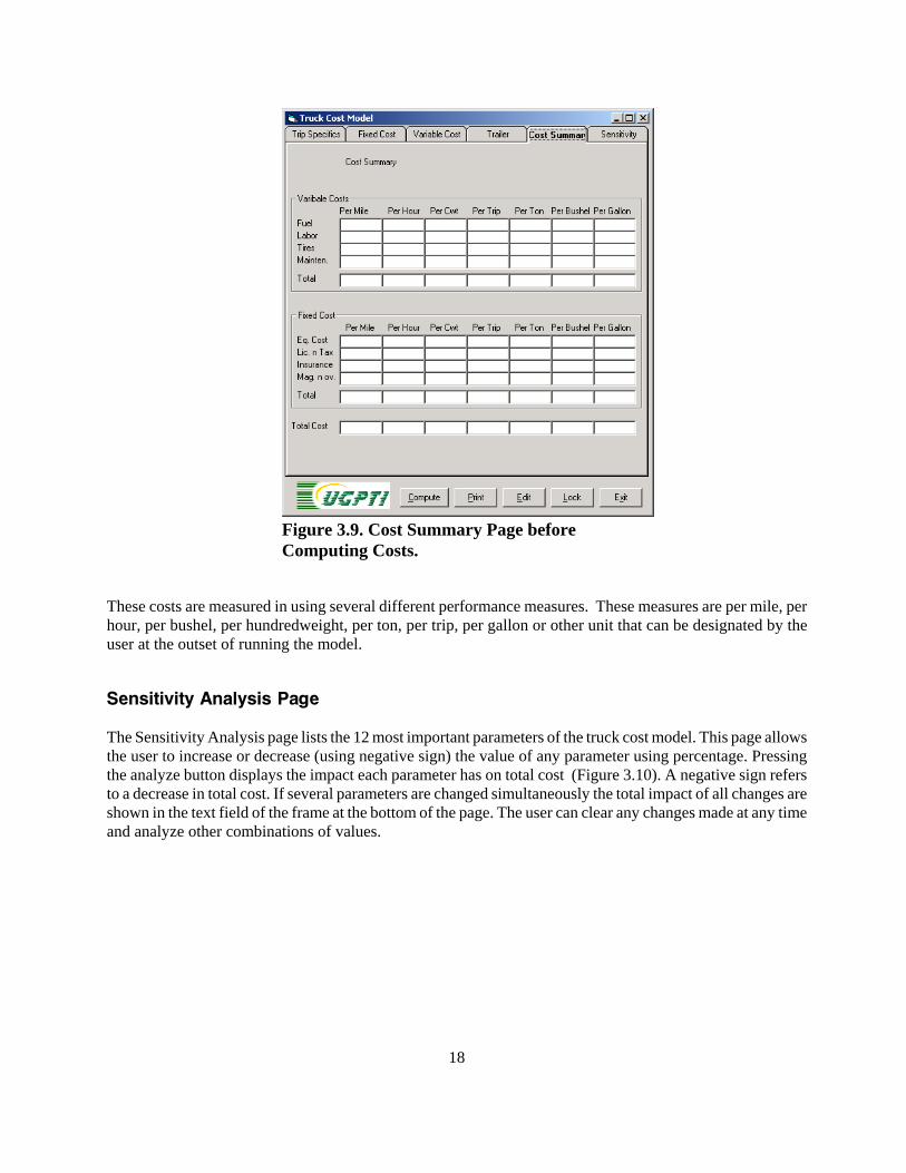
Figure 3.9. Cost Summary Page beforeComputing Costs.

These costs are measured in using several different performance measures. These measures are per mile, perhour, per bushel, per hundredweight, per ton, per trip, per gallon or other unit that can be designated by theuser at the outset of running the model.

Sensitivity Analysis Page

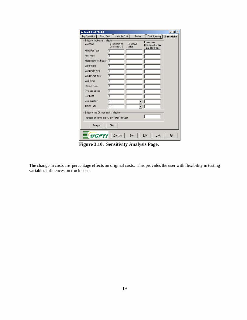
The Sensitivity Analysis page lists the 12 most important parameters of the truck cost model. This page allowsthe user to increase or decrease (using negative sign) the value of any parameter using percentage. Pressingthe analyze button displays the impact each parameter has on total cost (Figure 3.10). A negative sign refersto a decrease in total cost. If several parameters are changed simultaneously the total impact of all changes areshown in the text field of the frame at the bottom of the page. The user can clear any changes made at any timeand analyze other combinations of values.

19

Figure 3.10. Sensitivity Analysis Page.

The change in costs are percentage effects on original costs. This provides the user with flexibility in testingvariables influences on truck costs.

20

21

Figure 4.1. Trip Specifics Page after Calculatingthe Truck Costs.

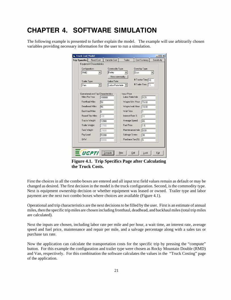
CHAPTER 4. SOFTWARE SIMULATION

The following example is presented to further explain the model. The example will use arbitrarily chosenvariables providing necessary information for the user to run a simulation.

First the choices in all the combo boxes are entered and all input text field values remain as default or may bechanged as desired. The first decision in the model is the truck configuration. Second, is the commodity type.Next is equipment ownership decision or whether equipment was leased or owned. Trailer type and laborpayment are the next two combo boxes where choices are available (Figure 4.1).

Operational and trip characteristics are the next decisions to be filled by the user. First is an estimate of annualmiles, then the specific trip miles are chosen including fronthaul, deadhead, and backhaul miles (total trip milesare calculated).

Next the inputs are chosen, including labor rate per mile and per hour, a wait time, an interest rate, averagespeed and fuel price, maintenance and repair per mile, and a salvage percentage along with a sales tax orpurchase tax rate.

Now the application can calculate the transportation costs for the specific trip by pressing the “compute”button. For this example the configuration and trailer type were chosen as Rocky Mountain Double (RMD)and Van, respectively. For this combination the software calculates the values in the “Truck Costing” pageof the application.

22

Figure 4.2. Variable Cost Page after Calculatingthe Truck Costs.

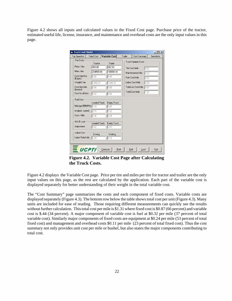
Figure 4.2 shows all inputs and calculated values in the Fixed Cost page. Purchase price of the tractor,estimated useful life, license, insurance, and maintenance and overhead costs are the only input values in thispage.

Figure 4.2 displays the Variable Cost page. Price per tire and miles per tire for tractor and trailer are the onlyinput values on this page, as the rest are calculated by the application. Each part of the variable cost isdisplayed separately for better understanding of their weight in the total variable cost.

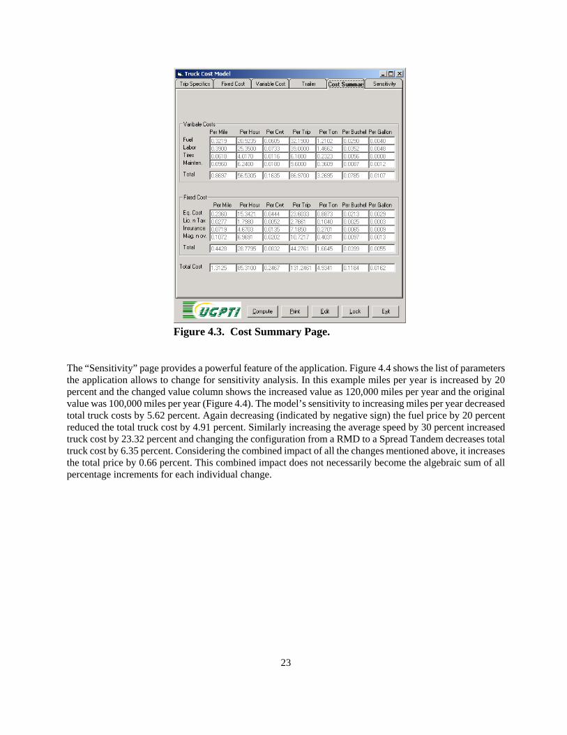
The “Cost Summary” page summarizes the costs and each component of fixed costs. Variable costs aredisplayed separately (Figure 4.3). The bottom row below the table shows total cost per unit (Figure 4.3). Manyunits are included for ease of reading. Those requiring different measurements can quickly see the resultswithout further calculation. This total cost per mile is $1.31 where fixed cost is $0.87 (66 percent) and variablecost is $.44 (34 percent). A major component of variable cost is fuel at $0.32 per mile (37 percent of totalvariable cost). Similarly major components of fixed costs are equipment at $0.24 per mile (53 percent of totalfixed cost) and management and overhead costs $0.11 per mile (23 percent of total fixed cost). Thus the costsummary not only provides unit cost per mile or bushel, but also states the major components contributing tototal cost.

23

Figure 4.3. Cost Summary Page.

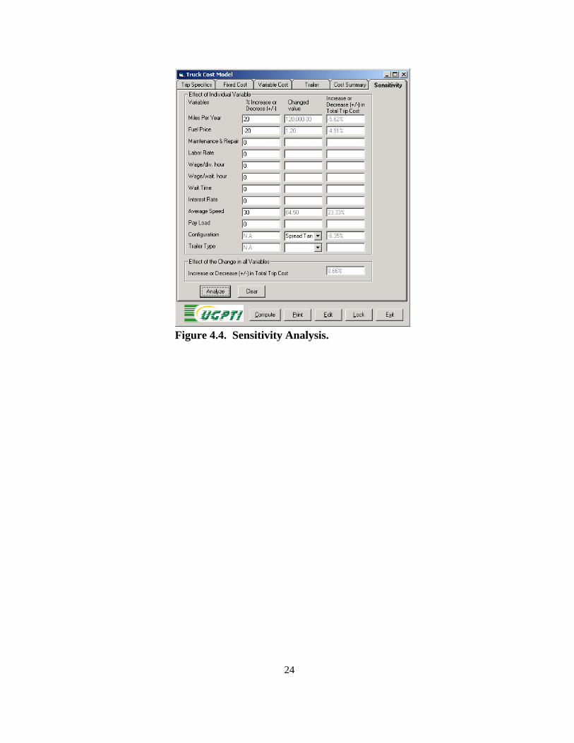
The “Sensitivity” page provides a powerful feature of the application. Figure 4.4 shows the list of parametersthe application allows to change for sensitivity analysis. In this example miles per year is increased by 20percent and the changed value column shows the increased value as 120,000 miles per year and the originalvalue was 100,000 miles per year (Figure 4.4). The model’s sensitivity to increasing miles per year decreasedtotal truck costs by 5.62 percent. Again decreasing (indicated by negative sign) the fuel price by 20 percentreduced the total truck cost by 4.91 percent. Similarly increasing the average speed by 30 percent increasedtruck cost by 23.32 percent and changing the configuration from a RMD to a Spread Tandem decreases totaltruck cost by 6.35 percent. Considering the combined impact of all the changes mentioned above, it increasesthe total price by 0.66 percent. This combined impact does not necessarily become the algebraic sum of allpercentage increments for each individual change.

24

Figure 4.4. Sensitivity Analysis.

25

CHAPTER 5. INPUT PRICES

Owner/operators face a competitive labor rate, which can be hourly, by the mile, or some combination. In thesoftware application, labor cost also can include wait time for loading and unloading. Wait time might beconsidered as an opportunity cost of operations and may be overlooked by many owner/operators.Owner/operators may not consider wait time or loading and unloading as a cost because of U.S. DOT rulesthat limit driving and on-duty time.

The interest rate is used for equipment purchase and leasing and also for return on investment (ROI). The ratevaries in the case of lease, or purchase, depending on the market rates and the risk factor foreseen by thelender. The rate can vary in the case of ROI depending on the return expected by the owner/operator.

The fuel price is an exogenous variable that depends on the current market rates for fuel. Fuel price may varydepending on geographical location, and supply and demand conditions. The default value is $1.50 per gallon.

Maintenance and repair costs are estimated at nine cents per vehicle mile and weight adjusted by .097 centsfor each 1,000 pounds above or below 58,000 pounds (Faucett and Associates, 1991). Technologicalimprovements and long warranties for trucks may lessen repair costs but individual firms will have differentmaintenance and repair costs depending on equipment and operating conditions. The default is set at ninecents and can be changed by the user.

Speed is a function of engine horsepower, terrain, wind, and weight. The model bases fuel economy on weightand speed. Ryder (1994) found that for every one mile-per-hour gain in speed above 55 miles per hour, fueleconomy drops 2 percent. As of the winter of 2002, industry experts concur that the fuel economy of the newtrucks are similar to results of the formulas developed for this software model. Many input fields have adefault value and the user is allowed to change these defaults before run time. The text fields for the valuesto be computed are kept empty and disabled (The page displays values in black which are input values and thevalues in gray are computed values).

Fixed Cost

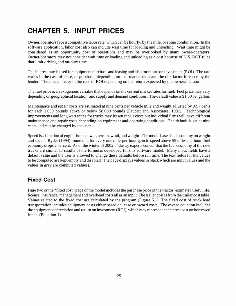
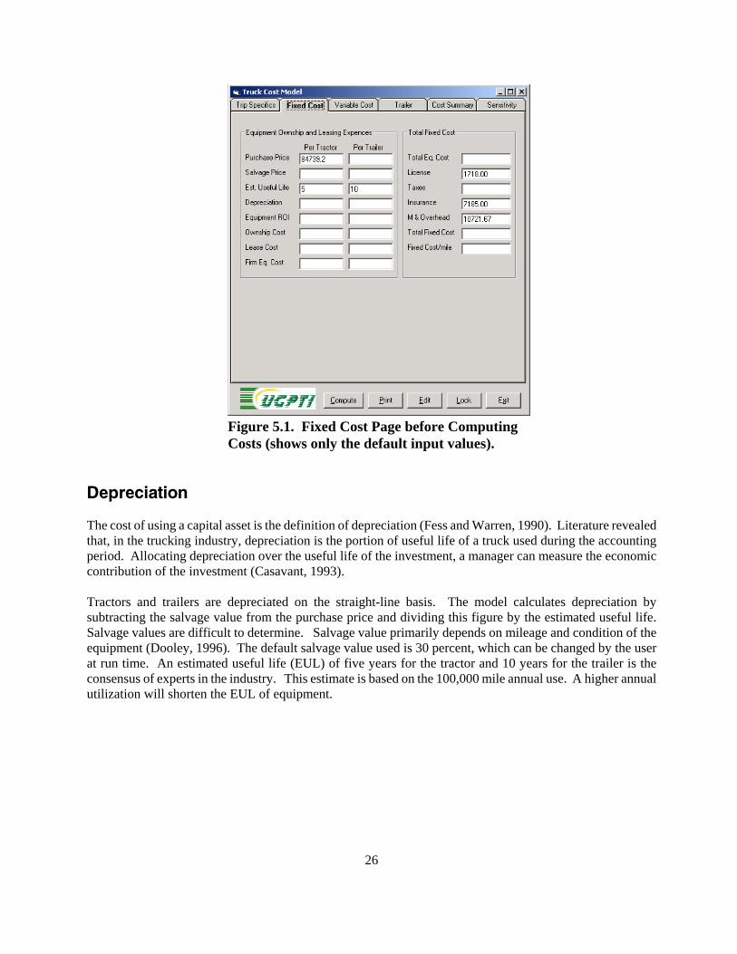
Page two or the “fixed cost” page of the model includes the purchase price of the tractor, estimated useful life,license, insurance, management and overhead costs all as an input. The trailer cost is from the trailer cost table.Values related to the fixed cost are calculated by the program (Figure 5.1). The fixed cost of truck loadtransportation includes equipment costs either based on lease or owned costs. The owned equation includesthe equipment depreciation and return on investment (ROI), which may represent an interest cost on borrowedfunds. (Equation 1).

26

Figure 5.1. Fixed Cost Page before ComputingCosts (shows only the default input values).

Depreciation

The cost of using a capital asset is the definition of depreciation (Fess and Warren, 1990). Literature revealedthat, in the trucking industry, depreciation is the portion of useful life of a truck used during the accountingperiod. Allocating depreciation over the useful life of the investment, a manager can measure the economiccontribution of the investment (Casavant, 1993).

Tractors and trailers are depreciated on the straight-line basis. The model calculates depreciation bysubtracting the salvage value from the purchase price and dividing this figure by the estimated useful life.Salvage values are difficult to determine. Salvage value primarily depends on mileage and condition of theequipment (Dooley, 1996). The default salvage value used is 30 percent, which can be changed by the userat run time. An estimated useful life (EUL) of five years for the tractor and 10 years for the trailer is theconsensus of experts in the industry. This estimate is based on the 100,000 mile annual use. A higher annualutilization will shorten the EUL of equipment.

27

Return On Investment

Equipment return on investment (ROI) constitutes another portion of equipment costs. ROI is considered tobe either interest on debt capital or return on equity investment. Therefore, Interest can be the desired returnof the manager or the rate paid on debt capital. The default value for interest is 11 percent and was estimatedas the interest rate a owner/operator may have to pay on borrowed capital for equipment (Equation 5.1).

Equation 5.1. Return on Investment.

where,

PP is purchase price, SV is savage value, and I is interest.

The program considers only one ownership cost or lease cost depending on the choice made on the TruckCosting page. Because the costing is for a particular trip, in the short run, truckers own or lease based on theirdecision at the time of acquiring the truck (Equations 5.2 and 5.3).

Equation 5.2. Total Equipment Cost (tractor and trailer)

Equipment ownership cost = Equipment depreciation + Equipment Return On Investment (ROI)

Equation 5.3. Total Equipment Lease Costs

Let:C = Cash Flow PaymentP = Principal (amount of loan of purchase price)I = yearly interest rate in decimalN = Number of years (period of lease)

Therefore,

C = (Pi) / [1 - (1 / (1 + I) N)]

PP-V2 + SV I

28

License Fees Insurance and Sales Tax

Other fixed costs associated with equipment are license fees and insurance. License fees and insurance area factor of trade area, miles traveled, weight, and product characteristics. Both have some characteristics ofvariable costs, but generally are treated as fixed costs (Casavant, 1993). License fees and fuel tax wereobtained from the N.D. Motor Vehicle Department in Bismarck and were prorated at $1,126. This fee is forboth North Dakota and Minnesota, where a vehicle would be used equally in both states. Insurance costs wereestimated to be $7,185 (Kleingartner, 2001). Estimates were obtained for a 350-mile radius of Fargo formovements in North Dakota and Minnesota. The model default is set at the aforementioned levels, but canbe changed in the model to reflect the user’s needs.

Sales tax also is a factor in the purchase of a new truck and trailer. This estimate is based on a percentage andthe purchase price of equipment. This is an entry the user can change in the model and the default is set at 5percent. This percentage varies on a per state basis.

Management and Overhead Costs

The literature described management and overhead costs as short-run fixed costs not directly attributable toa unit of output (Casavant, 1993). Dooley, Bertram, and Wilson (1988) identified management costs asmanagement and administration staff and overhead costs as advertising and communications equipment, officespace, and office equipment. For owner/operators, management and overhead costs may be minimal becausethe operator may be the manager and other costs are not applicable.

Management and overhead costs include costs for management and administrative help. Dooley, Bertram, andWilson (1988) reported that many owner/operators fail to allocate cost for management or administration.Overhead costs would include advertising and communications. Other costs included in management andoverhead are dispatch, sales, management, and accounting.

The default estimate for management and overhead is based on a Dooley, Bertram, and Wilson (1988) survey.The weighted average cost totaled $10,721 annually. Advances in technology may have lowered the costs ofcommunications and accounting. Cell phones can reduce the time spent in search for loads and dispatch, whilecomputers and electronic data communication can reduce time spent on accounting. This cost can be changedto reflect a company’s management cost.

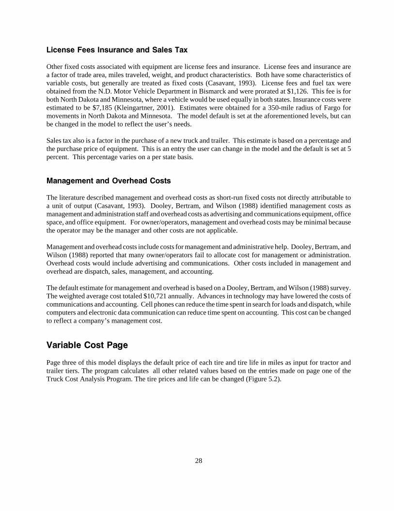
Variable Cost Page

Page three of this model displays the default price of each tire and tire life in miles as input for tractor andtrailer tiers. The program calculates all other related values based on the entries made on page one of theTruck Cost Analysis Program. The tire prices and life can be changed (Figure 5.2).

29

Figure 5.2. Variable Cost Page beforeComputing Costs (shows only the default inputvalues).

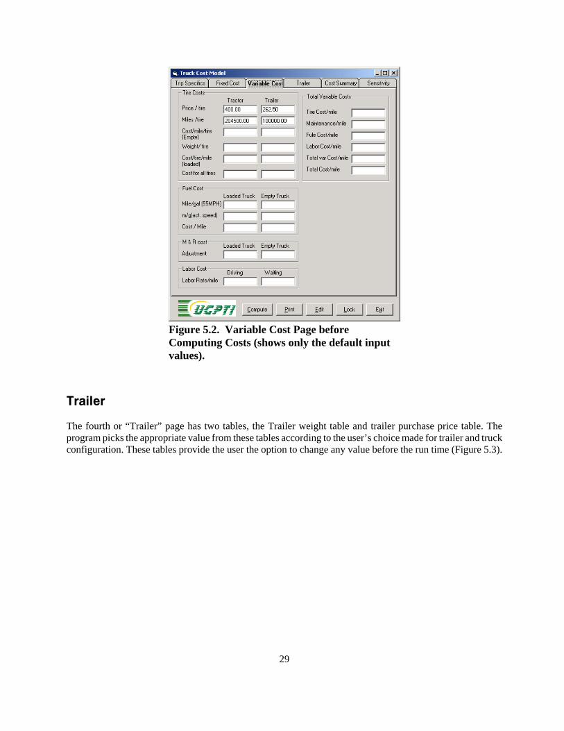
Trailer

The fourth or “Trailer” page has two tables, the Trailer weight table and trailer purchase price table. Theprogram picks the appropriate value from these tables according to the user’s choice made for trailer and truckconfiguration. These tables provide the user the option to change any value before the run time (Figure 5.3).

30

Figure 5.3. Trailer Weight and Purchase PriceTables in Trailer Page.

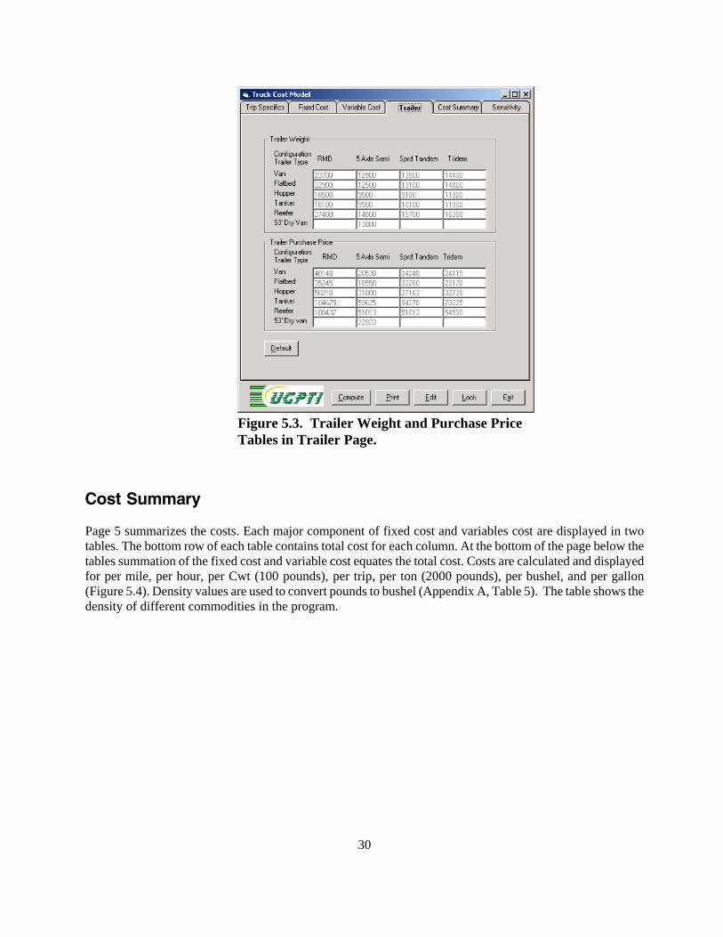
Cost Summary

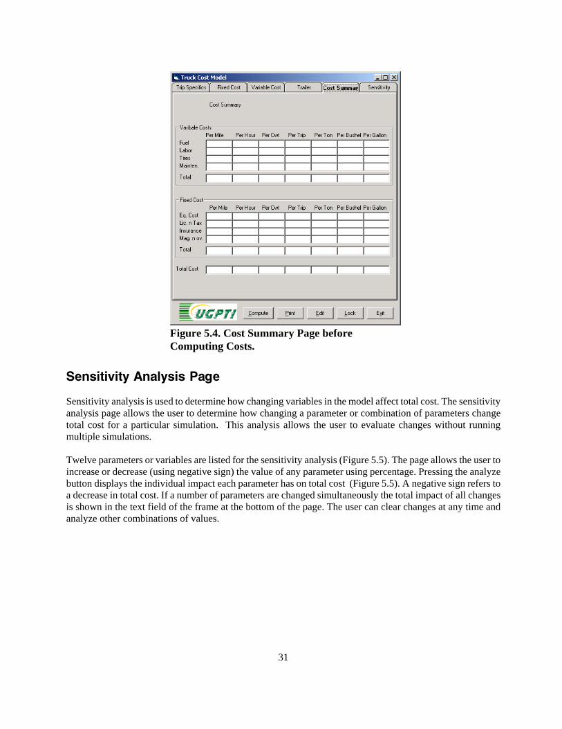
Page 5 summarizes the costs. Each major component of fixed cost and variables cost are displayed in twotables. The bottom row of each table contains total cost for each column. At the bottom of the page below thetables summation of the fixed cost and variable cost equates the total cost. Costs are calculated and displayedfor per mile, per hour, per Cwt (100 pounds), per trip, per ton (2000 pounds), per bushel, and per gallon(Figure 5.4). Density values are used to convert pounds to bushel (Appendix A, Table 5). The table shows thedensity of different commodities in the program.

31

Figure 5.4. Cost Summary Page beforeComputing Costs.

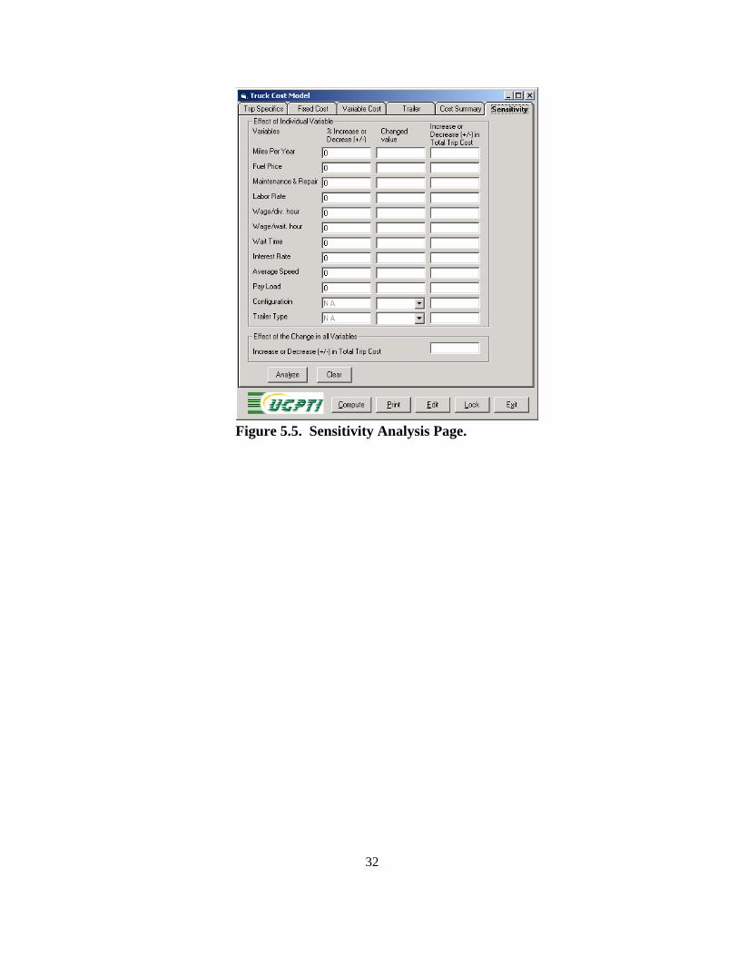
Sensitivity Analysis Page

Sensitivity analysis is used to determine how changing variables in the model affect total cost. The sensitivityanalysis page allows the user to determine how changing a parameter or combination of parameters changetotal cost for a particular simulation. This analysis allows the user to evaluate changes without runningmultiple simulations.

Twelve parameters or variables are listed for the sensitivity analysis (Figure 5.5). The page allows the user toincrease or decrease (using negative sign) the value of any parameter using percentage. Pressing the analyzebutton displays the individual impact each parameter has on total cost (Figure 5.5). A negative sign refers toa decrease in total cost. If a number of parameters are changed simultaneously the total impact of all changesis shown in the text field of the frame at the bottom of the page. The user can clear changes at any time andanalyze other combinations of values.

32

Figure 5.5. Sensitivity Analysis Page.

33

CHAPTER 6. CONCLUSIONS

Differences that exist among truck configurations, trip and product characteristics, and input prices influencecosts for individual owner/operators. Obtaining cost estimates for individual motor carrier movements isdifficult. The increasing need for on-time quality delivery of products makes it imperative for all users ofowner/operators to understand their costs. Shippers who understand that sustainability for the independenttrucker may reduce search costs for transportation and at the same time increase customer service by repeatedlyusing the same trucker. Also large trucking companies and or brokers who use owner/operators need truckcost information to benchmark performance against competitors and industry standards. The Truck CostingSoftware Model developed also may be used by shippers and owner/operators as a negotiating tool to arriveat equitable shipping rates.

An Owner/Operator Spreadsheet Costing Model developed in 1996 has been useful, however it is based ona spreadsheet and is not a stand alone model or software product. The software model developed is to be astand alone product that does not require any specific software applications except for Microsoft Windows.The model includes many truck configurations, freight options, and performance measures.

Performance Measures

Previous motor carrier cost studies focused on per mile costs. Users of independent truckers may use differentperformance measures for the same movement. A shipper may measure costs in units, while the truckermeasures in miles. This study differs from the previous studies in the performance measures provided and alsoflexibility of the model.

The objective of this study was to provide truck cost information to reflect differences in equipment,product, and trip characteristics of an individual firm. The secondary objective was to provideadditional performance measures for decision makers who need owner/operator cost information.The measures include, but are not limited to:

• cost per mile• cost per bushel• cost per hundredweight• cost per ton• cost per trip• cost per hour• cost per gallon• cost per unit

Development and Data

The model is implemented using Visual Basic, a widely used programming language. Visual Basic allows aprogrammer to develop applications with graphical user interfaces that run in Microsoft’s Windows withoutthe complexity generally associated with Windows programming. This application includes three forms; asplash screen form, a main form, and a small pop up form used to add new commodity type or unit.

34

Data used to build the model came from a combination of previous studies, interviews, and journal articles.Information used from previous studies was updated and verified through interviews of industry experts.Estimates on license fees and taxes came from the N.D. Department of Motor Vehicles. Estimates oninsurance were received from West Fargo Insurance. Equipment quotes came from Wallwork Truck Sales andJohnson Trailer Sales. Tire cost estimates were received from OK Tire, with costing and wear information.

Assumptions and Operating Characteristics

The operating characteristics of the firm assumed 100,000 mile equipment usage. A simulation of the modelused an equipment configuration of an RMD setup pulling a 48-foot van with a 28-foot pup trailer and a GVWof 90,800 pounds and a payload of 53,200 pounds. Capital equipment costs were estimated to be $84,739 forthe tractor and $40,180 for the trailer, with an estimated useful life of five years for the truck and 10 years forthe trailer. The equipment was assumed to be purchased rather than leased.

Industry estimates for labor rates of non-refrigerated, non-union wages at 29 cents per mile. Default laborcost was 29 cents per mile. The interest rate estimate of 11 percent may be on the high end of the range ofrates a new owner/operator may have to pay because of the risk factor associated with independent truckers.Only one interest rate was used in the model. The rate of 11 percent was used for return on investment andcomputing lease payments. Functions of fuel costs include fuel price, weight, speed, terrain, and truckconfiguration. Fuel costs are determined from a coefficients table for different truck configurations and trailertypes developed by David Knapton (Faucett and Associates, 1991). The assumptions made in using the tableare for level terrain 55 miles per hour and fuel-efficiency options in use in 1985. Ryder (1994) confirmed thatnot only is fuel efficiency weight sensitive, but also speed sensitive. The estimation in the article is that forevery mile per hour over 55, there is a 2 percent loss in fuel efficiency. The embedded formula in the modeluses the coefficients table for weight and adjusts automatically for speed over 55 miles per hour. The basecase for the RMD at 65 miles per hour results in miles per gallon of 4.15 loaded and 5.34 empty. This estimatewas confirmed to be a good estimation of fuel economy by industry experts. The model estimates fuel mileagefor a five-axle semi at 80,000 GVW and 55 mph at 7.73 miles per gallon empty and 5.72 miles per gallonloaded.

The base maintenance and repair costs are nine cents per mile with a load factor of plus or minus .097 centsper mile per 1,000 pounds of weight over or under 58,000 pounds. Faucett and Associates (1991) estimatedmaintenance and repair costs at 10 cents per mile with a .108 cents per mile change per 1,000 pounds changein gross vehicle weight. Better warranties have brought repair costs down for many trucking firms. The ageof the equipment and operating conditions directly impact maintenance and repair costs. The model wassimulated with a base maintenance cost of nine cents. All variables can be changed by the user to reflectoperating conditions and actual available data.

Tire costs were weight adjusted with different mileage estimations for tractor and trailer tires. Tractor tiresare estimated to cost $400 with estimated mileage of 204,500 miles, while trailer tires are estimated to cost$262.50 with expected mileage of 100,000 miles. Tires wear more with more weight, and some trailerconfigurations have more tire wear. Data suggest that for a five-axle semi above 3,500 pounds per tire, tirelife decreases by about .7 percent for each 1 percent increase in weight (Faucett and Associates, 1991). Forthe base case scenario, tire costs are estimated at 4.5 cents per mile, which includes the load factor.

35

Flexibility of the Model

The model was designed for ease of use and can quickly provide results for different configurations and bodytypes. “SStabs” were used in programming to provide for ease of jumping back and forth among the pagesin the model.

The decision maker can choose the interest rate, fuel price, labor rate, payload, and trip design. Thesevariables all are easily changed to compensate for different truck and trip characteristics. The model is easilyupdated. Equipment costs and other factors, such as tire price or insurance costs, can be changed. All partsof the model easily are changed to specific applications. Performance measures can be added to fit differentsituations.

Results

The end results of running a simulation are the performance measures in costs per mile, hour, bushel, hundredweight, ton, and trip. These costs are separated into fixed and variable cost categories. Variable costcategories include fuel, labor, tires, and maintenance and repair. Fixed costs categories include equipment,license fees and taxes, management and overhead, and insurance.

Sensitivity

Sensitivity analysis can be performed on variables that may change. Variables, such as wages, fuel price,maintenance and repair, or equipment utilization, may be different or changing for individual owner/operators.Analysis can easily be run by using the sensitivity analysis section of the model to quickly access an increaseor decrease in fuel prices or a change in equipment usage.

Summary

Truckers face different input prices, product characteristics, truck configurations, geographical characteristics,firm size, and driving practices. Thus, obtaining current estimates of costs for particular independentowner/operators is difficult. The software that was developed determines costs for a variety of truckconfigurations, product characteristics, and input prices. A firm's costs are determined by its equipment,characteristics of products hauled, and input prices associated with a typical movement for that firm.

The truck costing software may provide information to many in the trucking and or shipping industry. Anyoneestimating transportation costs needs reliable estimates of owner/operator costs. Also some shippers needaccurate truck cost information to negotiate desirable rates and determine the appropriate mode oftransportation.

A stand-alone Truck Costing Model was developed using Microsoft Visual Basic for Windows. The modelin this study has many useful features. Costs can be obtained for many different configurations and tripcharacteristics. Important conclusions can be drawn from running simulations include the sensitivity of costsand equipment use, wait time and trip distance, labor, and fuel price. The relationships of these variables andthe cost of operations are important for trucking interests.

36

The simulations and sensitivity analysis determined the truck cost model's flexibility and inadequacies.Factors influencing costs of owner/operators include annual miles, trip distance, and truck speed for fuelefficiency. Decreasing annual miles may be critical for the trucker debating on waiting for a better revenueload. The opportunity cost of waiting may more than make up for the additional revenue received. Anotherinteresting factor in the model is the wait time. Initial assumptions exclude wait time, but loading andunloading time for short movements are the driving force of increased costs. The shorter the trip, the greaterthe impact of loading and unloading time on cost.

37

REFERENCES

Battelle Team (1995). Comprehensive Truck Size and Weight Study. Federal Highway AdministrationDepartment of Transportation. Working Paper 7. Washington, District of Columbia.

Benson, P. (2002). Interview for Interest Rates. First Bank Systems. Fargo, North Dakota.

Bierman, H., Bonini, C., & Hausman, W. (1991). Quantitative Analysis for Business Decisions. 8th ed. Richard D. Irwin Inc., Homewood, Illinois.

Casavant, K. (1993). Basic Theory of Calculating Costs: Applications to Trucking. Upper Great PlainsTransportation Institute No. 118. North Dakota State University. Fargo.

Coyle, J., Bardi, E., & Novack, R. (1994). Transportation. West Publishing Company, St. Paul, Minnesota.

Crum, M., Premkumar, G., & Ramamurthy, K. (1996). "An Assessment of Motor Carrier Adoption, Use, andSatisfaction with EDI." Transportation Journal. Summer 1996.

Dooley, F., Bertram, L., & Wilson,W. (1988). Operating Costs and Characteristics of North Dakota GrainTrucking Firms. Upper Great Plains Transportation Institute No. 67. North Dakota State University.Fargo.

Dooley, F. (1991). Economies of Size and Density for Short Line Railroads. Mountain Plains ConsortiumNo. 91-2. Upper Great Plains Transportation Institute. North Dakota State University. Fargo.

Dooley, F., & Wilson,W. (1991). An Empirical Examination of Market Access. Upper Great Plains

Transportation Institute No. 106. North Dakota State University. Fargo, North Dakota.

Dooley, T. (1996). Interview for Trucking Characteristics. Wallwork Truck Sales. Fargo, North Dakota.

Faucett & Associates (1991). The Effect of Size and Weight Limits on Truck Costs. Bethesda, Maryland.

Ferguson, C., & Gould, J. (1975). Microeconomic Theory. Richard D. Irwin Inc., Homewood, Illinois.

Ferguson, C., & Kreps, J. (1965). Principles of Economics. Holt, Rinehart, & Winston Inc., New York.

Fess, P., & Warren, W. (1990). Accounting Principles. South-Western Publishing Company, Cincinnati,Ohio.

Griffin, G., & Rodriguez, J. (1992). Creating a Competitive Advantage Through Partnershipping WithOwner-Operators. Upper Great Plains Transportation Institute No. 91. North Dakota StateUniversity. Fargo.

Griffin, G., Rodriguez, J., & Lantz, B. (1992). Evaluation of the Impact of Changes in the Hours of ServiceRegulations on Efficiency, Drivers and Safety. Upper Great Plains Transportation Institute No. 93.North Dakota State University. Fargo, North Dakota.

Heggeness, J. (2002). Interview for Tire Pricing and Mileage. OK Tire Store. Fargo, North Dakota.

38

Hesh, R. (2002). Interview for Truck Prices. Wallwork Truck Sales. Fargo, North Dakota.

Hirschey, M., & Pappas J. (1993). Managerial Economics. 7th ed. The Dryden Press. Harcourt BraceJovanovich College Publishers, Orlando, Florida.

Kapel, J. (2002). Interview for Trailer Costs. Johnson Trailer Sales. Fargo, North Dakota.

Kleingartner, J. (2002). Interview for Insurance Costs. West Fargo Insurance. West Fargo, North Dakota.

Knapton, D. (1981). Truck and Rail Fuel Effects of Truck Size and Weight Limits. U.S. Department ofTransportation. Transportation Systems Center, Cambridge, Massachusetts.

Maurice, C., & Phillips, O. (1992). Economic Analysis: Theory and Application. 6th ed. Richard D. IrwinInc., Homewood, Illinois.

McConnell, C., & Brue, S. (1990). Economics: Principles, Problems, And Policies. 11th ed. McGraw-HillPublishing Company, San Francisco, California.

Nicolson, W. (1995). Microeconomic Theory: Basic Principles and Extensions. 6th ed. The Dryden Press.Hartcourt Brace & Company, Orlando, Florida.

Ryder, A. (1994). "Fuel-Efficient Driving: The Basics." Heavy Duty Trucking 73 (7).

Skager, C. (2002). Interview for License and Fees. North Dakota State Motor Vehicle Department. Bismarck.

Titus, M. (1994). Implications of Electronic Clearance for Regulatory Enforcement of Trucking Industry. Upper Great Plains Transportation Institute No. 103. North Dakota State University. Fargo.

Truck Size and Weight and User Fee Policy: Analysis Study for U.S. Department of Transportation FederalHighway Administration. Washington, District of Columbia.

Vachal, Kimberly (2001). North Dakota Grain and Oilseed Transportation Statistics. Upper Great PlainsTransportation Institute. North Dakota State University. Fargo.

39

APPENDIX A. DETAILED CALCULATIONS OF THEMODEL

This section will show calculations in the Truck Cost Analysis Software, which determines variable and fixedcosts. The costs are segmented in fixed and variable costs by their components. The calculations will beshown by those components.

Variable Cost Components

The components making up variable costs, as mentioned previously are fuel, labor, tires, and maintenance andrepair. The calculations for these individual components will be explained. In order to provide an examplefor variable cost components the derivation of gross vehicle weight is explained.

GVW

INPUT:Pay Load = 53,200 lb (determined by the user of the model)Tractor weight = 13900 lbTrailer weight = 23700 lb (Appendix I)

CALCULATE:

Tare weight = Trailer weight + Tractor weight = (23700 + 13900) lbs

= 37,600 lb

Gross Vehicle weight, GVW = (Pay Load + Tare weight) = (53,200 + 37,600) lb= 90,800 lb

Fuel

The fuel price is an exogenous variable that depends on the current market rates. Fuel price may varydepending on geographical location and supply and demand conditions. Fuel economy is a function of enginehorsepower, speed, terrain, wind, and weight. At the same time speed is a function of engine horsepower, terrain, wind and weight. This study based fuel economy on weight and speed. Ryder (1994) found that forevery one mile per hour gain in speed over 55 miles per hour, fuel economy drops 2 percent. KnaptonsFormula is based on the co-efficient table and may be adjusted for speed. The following procedure shows thecalculations.

40

Where:

FC is a fixed co-efficientGVW is gross Vehicle WeightVC is a variable co-efficientINPUT:

MPH = average speed = 65 miles/hourFuel Price= 1.50

Calculate Loaded Truck:For RMD and Van FC = 0.1203 (From Table, Appendix I ) For RMD and Van VC = 0.0008 (From Table, Appendix I)Loaded GVW = 90,800 (calculated)Empty GVW = Tare weight = 37,600 (From Table, Appendix I)

Calculated For Empty Truck:Speed = 65 MPH; [0.02*(MPH -55)] = 0.2

For loaded truck = 5.182985(1 – 0.2) miles/ gallon= 4.1464 miles/gallon

For empty truck = 6.64982(1 – 0.2) miles/ gallon= 5.3199 miles/gallon time loaded = 50% [previous input]

% time Empty = 50 %

Cost/mile for fuel (Loaded truck) = (Fuel Price/ gallon)/ (miles/gallon)= 1.5/4.1464 = 0.3618 / mile

Cost/mile for fuel (Empty truck) = (Fuel Price/ gallon)/ (miles/gallon)= 1.5/5.3199 = 0.2820 / mile

Average fuel cost/mile = (Loaded cost*Time Loaded + Empty cost*time empty)= 0.3618*0.5 + 0.2820*0.5= 0.3219 /mile

Labor

Rates for labor is a readily known variable for paid drivers and is accounted for in the model by per time andper mile. The user of the model can choose per mile, per hour, or both.The model is designed to recognize wages through the initial entry on sheet one. If functions are used to placelabor costs into the performance measures:

If(LM>0andWT=0,LM)If(LM>0andWT>0,(LM+((TD/S)+WT)*LH))/TD))If(LM=0,((TD/S)+WT)*LH)/TD))

41

where:

LM=Labor Rate Per MileTD=Trip DistanceWT=Wait TimeLH=Labor Rate Per HourS=Speed

=(.29+(((100/65)+1)*10))/100)=$.39/mile

Tire Cost

The combination of tire price and tire wear make up tire costs. Tires are weight sensitive and wear more withmore weight. Tire life is independent of weight below 3,500 pounds per tire (Faucett and Associates, 1991).Weights above 3,500 pounds result in a .7 increase in wear for each 1 percent increase in weight.

INPUT:

Tractor tires cost/ tire = 400.00Trailer tires cost/ tire = 262.50Tractor tires miles/ tire = 204500.00Trailer tires miles/ tire = 100000.00

Tire cost is independent of weight below 3500 lb/tire

GVW/(number of tractor tires + number of trailer tires) > 35000.7 % increase in cost for each 1% increase in weight

Tire cost increase/mile = (GVW/tire – 3500)/3500*100*0.007*Tractor tire cost/mile

Increased Tire cost/mile = (Tire cost/tire)/(Tire miles/tire) + [Increment if GVW/tire>3500]

Tire cost/ truck = (Loaded tire cost/mile/time)*(Num of tires)*Percent time loaded + (Empty tire cost/mile/time)*(Num of tires)*Percent time empty

In this example:

Empty tire cost/mile/tire for tractor = 400.00/204500 = 0.00195599Empty tire cost/mile/tire for trailer = 265.50/100000 = 0.002625For RMD & VanNumber of Tractor Tires = 10Number or Trailer Tires = 16Number of Total Tires = 26

42

Loaded GVW = 90800Empty GVW = 37600

90800/26 = 3492.3 < 3500

So no incrementLoaded tire cost/mile/tire for tractor = 0.00195599Loaded tire cost/mile/tire for trailer = 0.002625Percent Loaded = 50% [Previously calculated]Percent Empty = 50% [Previously calculated]

Tire cost/vehicle/mile for Tractor = (Loaded tire cost/mile/time)*(Num of tires)*Percent time loaded

+ (Empty tire cost/mile/time)*(Num of tires)*Percent time empty= 0.00195599*10*0.5 + 0.00195599*10*0.5= 0.00195599

Tire cost/vehicle/mile for Trailer= 0.002625*16*0.5 + 0.002625*16*0.5= 0.042

Total Tire cost /vehicle/mile= Cost for tractor tire + Cost for Trailer tires= 0.00195599 + 0.042= $.06155/mile

Maintenance and Repair Cost

Maintenance and repair is based on a formula from Faucett and Associates (1991) where a scaling procedurewas used. The formula is weight sensitive and is based on a gross vehicle weight (GVW) of 58,000 pounds.Service costs are nine cents per vehicle mile and weight adjusted by .097 cents for each 1,000 pounds aboveor below 58,000 pounds (Faucett and Associates, 1991). Long warranties exist for major components ontractors, so maintenance and repair costs vary depending on the age of the equipment, weight and operatingconditions. Base cost = 0.09 per mile

Weight adjustment: +-0.097 cents for each 1000 pounds above or below 58,000

Maintenance and repair

cost/mile = 0.09 + adjustment

Adjustments:For Loaded truck = ((Loaded GVW - 58000)/1000)*0.00097* Percent time loadedFor Empty truck = ((58000 – Empty GVW )/1000)*0.00097* Percent time empty

In this example: Loaded GVW = 90800Empty GVW = 37600

43

Percent time loaded = 50%Percent time empty = 50%

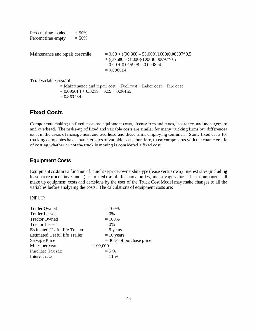
Maintenance and repair cost/mile = 0.09 + ((90,800 – 58,000)/1000)0.00097*0.5+ ((37600 – 58000)/1000)0.00097*0.5= 0.09 + 0.015908 – 0.009894 = 0.096014

Total variable cost/mile = Maintenance and repair cost + Fuel cost + Labor cost + Tire cost= 0.096014 + 0.3219 + 0.39 + 0.06155= 0.869464

Fixed Costs

Components making up fixed costs are equipment costs, license fees and taxes, insurance, and managementand overhead. The make-up of fixed and variable costs are similar for many trucking firms but differencesexist in the areas of management and overhead and those firms employing terminals. Some fixed costs fortrucking companies have characteristics of variable costs therefore, those components with the characteristicof costing whether or not the truck is moving is considered a fixed cost.

Equipment Costs

Equipment costs are a function of: purchase price, ownership type (lease versus own), interest rates (includinglease, or return on investment), estimated useful life, annual miles, and salvage value. These components allmake up equipment costs and decisions by the user of the Truck Cost Model may make changes to all thevariables before analyzing the costs. The calculations of equipment costs are:

INPUT:

Trailer Owned = 100%Trailer Leased = 0%Tractor Owned = 100%Tractor Leased = 0%Estimated Useful life Tractor = 5 yearsEstimated Useful life Trailer = 10 yearsSalvage Price = 30 % of purchase priceMiles per year = 100,000Purchase Tax rate = 5 %Interest rate = 11 %

44

CALCULATE:

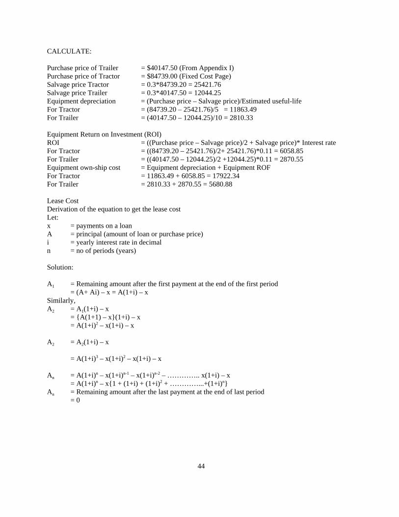
Purchase price of Trailer = $40147.50 (From Appendix I)Purchase price of Tractor = $84739.00 (Fixed Cost Page)Salvage price Tractor = 0.3*84739.20 = 25421.76Salvage price Trailer = 0.3*40147.50 = 12044.25Equipment depreciation = (Purchase price – Salvage price)/Estimated useful-lifeFor Tractor = (84739.20 – 25421.76)/5 = 11863.49For Trailer = (40147.50 – 12044.25)/10 = 2810.33

Equipment Return on Investment (ROI)ROI = ((Purchase price – Salvage price)/2 + Salvage price)* Interest rateFor Tractor = ((84739.20 – 25421.76)/2+ 25421.76)*0.11 = 6058.85 For Trailer = ((40147.50 – 12044.25)/2 +12044.25)*0.11 = 2870.55Equipment own-ship cost = Equipment depreciation + Equipment ROFFor Tractor = 11863.49 + 6058.85 = 17922.34For Trailer = 2810.33 + 2870.55 = 5680.88

Lease CostDerivation of the equation to get the lease costLet:x = payments on a loanA = principal (amount of loan or purchase price)i = yearly interest rate in decimaln = no of periods (years)

Solution:

A1 = Remaining amount after the first payment at the end of the first period= (A+ Ai) – x = A(1+i) – x

Similarly, A2 = A1(1+i) – x

= {A(1+1) – x}(1+i) – x = A(1+i)2 – x(1+i) – x

A2 = A2(1+i) – x

= A(1+i)3 – x(1+i)2 – x(1+i) – x

An = A(1+i)n – x(1+i)n-1 – x(1+i)n-2 – ………….. x(1+i) – x = A(1+i)n – x{1 + (1+i) + (1+i)2 + …………...+(1+i)n}

An = Remaining amount after the last payment at the end of last period = 0

45

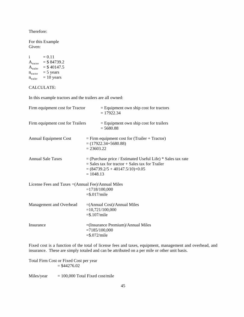
Therefore: For this Example Given:

i = 0.11Atractor = $ 84739.2Atrailer = $ 40147.5ntractor = 5 yearsntrailer = 10 years

CALCULATE:

In this example tractors and the trailers are all owned:

Firm equipment cost for Tractor = Equipment own ship cost for tractors= 17922.34

Firm equipment cost for Trailers = Equipment own ship cost for trailers= 5680.88

Annual Equipment Cost = Firm equipment cost for (Trailer + Tractor)= (17922.34+5680.88)= 23603.22

Annual Sale Taxes = (Purchase price / Estimated Useful Life) * Sales tax rate= Sales tax for tractor + Sales tax for Trailer= (84739.2/5 + 40147.5/10)+0.05= 1048.13

License Fees and Taxes =(Annual Fee)/Annual Miles=1718/100,000=$.017/mile

Management and Overhead =(Annual Cost)/Annual Miles=10,721/100,000=$.107/mile

Insurance =(Insurance Premium)/Annual Miles=7185/100,000=$.072/mile

Fixed cost is a function of the total of license fees and taxes, equipment, management and overhead, andinsurance. These are simply totaled and can be attributed on a per mile or other unit basis.

Total Firm Cost or Fixed Cost per year= $44276.02

Miles/year = 100,000 Total Fixed cost/mile

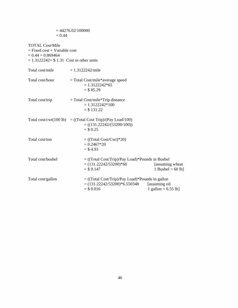
46

= 44276.02/100000= 0.44

TOTAL Cost/Mile = Fixed cost + Variable cost= 0.44 + 0.869464= 1.3122242= $ 1.31 Cost in other units

Total cost/mile = 1.3122242/mile

Total cost/hour = Total Cost/mile*average speed= 1.3122242*65= $ 85.29

Total cost/trip = Total Cost/mile*Trip distance= 1.3122242*100= $ 131.22

Total cost/cwt(100 lb) = ((Total Cost Trip)/(Pay Load/100)= ((131.22242/(53200/100))= $ 0.25

Total cost/ton = ((Total Cost/Cwt)*20)= 0.2467*20= $ 4.93

Total cost/bushel = ((Total Cost/Trip)/Pay Load)*Pounds in Bushel= (131.22242/53200)*60 [assuming wheat = $ 0.147 1 Bushel = 60 lb]

Total cost/gallon = ((Total Cost/Trip)/Pay Load)*Pounds in gallon= (131.22242/53200)*6.550348 [assuming oil = $ 0.016 1 gallon = 6.55 lb]

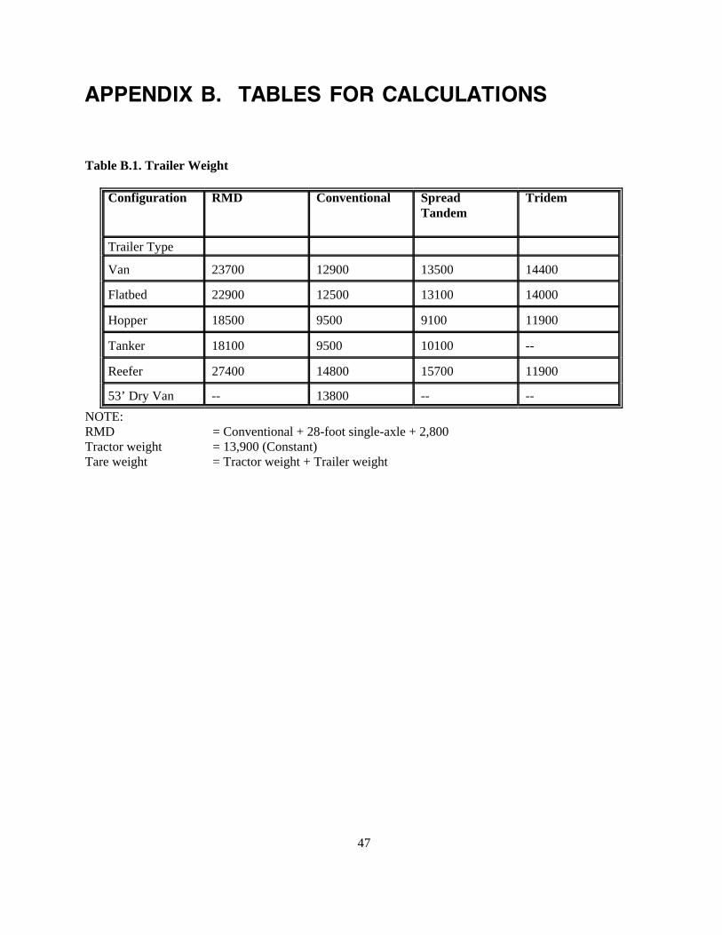
47

APPENDIX B. TABLES FOR CALCULATIONS

Table B.1. Trailer Weight

Configuration RMD Conventional SpreadTandem

Tridem

Trailer Type

Van 23700 12900 13500 14400

Flatbed 22900 12500 13100 14000

Hopper 18500 9500 9100 11900

Tanker 18100 9500 10100 --

Reefer 27400 14800 15700 11900

53’ Dry Van -- 13800 -- --NOTE:RMD = Conventional + 28-foot single-axle + 2,800Tractor weight = 13,900 (Constant)Tare weight = Tractor weight + Trailer weight

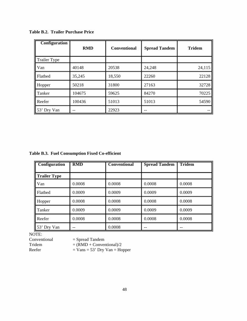
48

Table B.2. Trailer Purchase Price

ConfigurationRMD Conventional Spread Tandem Tridem

Trailer Type

Van 40148 20538 24,248 24,115

Flatbed 35,245 18,550 22260 22128

Hopper 50218 31800 27163 32728

Tanker 104675 59625 84270 70225

Reefer 100436 51013 51013 54590

53’ Dry Van -- 22923 -- --

Table B.3. Fuel Consumption Fixed Co-efficient

Configuration RMD Conventional Spread Tandem Tridem

Trailer Type

Van 0.0008 0.0008 0.0008 0.0008

Flatbed 0.0009 0.0009 0.0009 0.0009

Hopper 0.0008 0.0008 0.0008 0.0008

Tanker 0.0009 0.0009 0.0009 0.0009

Reefer 0.0008 0.0008 0.0008 0.0008

53’ Dry Van -- 0.0008 -- --NOTE:Conventional = Spread TandemTridem = (RMD + Conventional)/2Reefer = Vans = 53’ Dry Van = Hopper

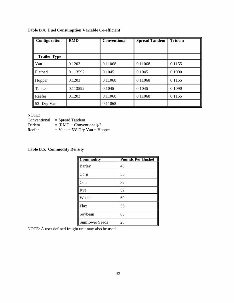
49

Table B.4. Fuel Consumption Variable Co-efficient

Configuration RMD Conventional Spread Tandem Tridem

Trailer Type

Van 0.1203 0.11068 0.11068 0.1155

Flatbed 0.113592 0.1045 0.1045 0.1090

Hopper 0.1203 0.11068 0.11068 0.1155

Tanker 0.113592 0.1045 0.1045 0.1090

Reefer 0.1203 0.11068 0.11068 0.1155

53’ Dry Van 0.11068

NOTE:Conventional = Spread TandemTridem = (RMD + Conventional)/2Reefer = Vans = 53’ Dry Van = Hopper

Table B.5. Commodity Density

Commodity Pounds Per BushelBarley 48

Corn 56

Oats 32

Rye 52

Wheat 60

Flax 56

Soybean 60

Sunflower Seeds 28NOTE: A user defined freight unit may also be used.

50

51

APPENDIX C. FIXED AND VARIABLE COSTS

Costs identified in the literature review include fixed and variable costs components for an owner/operator.Fixed costs are costs that do not change with output and cannot be changed quickly or in the short run. Theshort run is a period in which a firm cannot change its factors of production. Variable costs change with outputand may be easily changed (Ferguson and Kreps, 1965). The distinguishing characteristic between fixed andvariable cost is time. In the long run, all costs are variable, or can be changed.

Dooley, Bertram, and Wilson (1988), Casavant (1993), and Faucett and Associates (1991) identified costsincurred by trucking firms. Variable costs are costs that can be attributed to mileage, or running time (Dooley,Bertram, and Wilson, 1988). The literature revealed that owner/operator variable costs include maintenanceand repair, fuel, labor, and tires. Fixed costs are incurred whether or not a truck is logging miles (Dooley,Bertram, and Wilson, 1988). Items of fixed costs include equipment costs, license fees and taxes, insurance,and management and overhead.

Operational trade-offs exist between large and small carriers. Small firms may be free from many costsassociated with larger firms such as terminal operations, administrative and management specialists, andinformation systems; but larger firms may enjoy an advantage in purchasing sophisticated technology,equipment, and other inputs where large volume discounts may exist (Coyle, Bardi, and Novak, 1994).

Even though it appears economic gains from size are minimal, there are many small companies owning morethan a single power unit or trailer. It would be intuitive to assume that some economies could be gained in theform of volume discounts for some inputs used in the trucking industry for those operating more than onepower unit. However, in the truckload sector of the trucking industry, there does not seem to be any majoreconomies due to the size of a company (Coyle, Bardi, and Novak, 1994). The large number of small firmsoperating in the motor carrier industry should attest that economies of size are not extensive.

Economies of Utilization

Owner/operators may not incur some fixed costs associated with larger firms. While economies of size areminimal for the owner/operator, economies of utilization are possible. C o s t m i n i mi z a t i o n f o r t h eowner/operator encourages high usage of equipment. The concept of economies of utilization is allocationof fixed costs over increased output and is realized by increasing the use of those fixed assets. Equipmentusage for owner/operators may be limited by the hours of service allowed by federal regulations (Griffin,Rodriguez, and Lantz, 1992).

Opportunity exists for the entrepreneur who employs a strategy of increased equipment use. Increasedequipment usage may be accomplished by adding a driver and using a team concept. Additional revenue fromincreased equipment use may more than offset higher labor and other increased costs by decreasing fixed costsand total costs per unit of output. Figure 1 shows the cost relationship with increased use. As usage increases,average fixed cost per unit decreases.

Figure 1 shows the average fixed cost curve slopes downward throughout the entire range. As outputapproaches zero, average fixed cost becomes larger and larger, but as output increases, average fixed costbecomes smaller and smaller. Thus, Figure 1 depicts the concept of increased equipment use to minimizeaverage total costs.

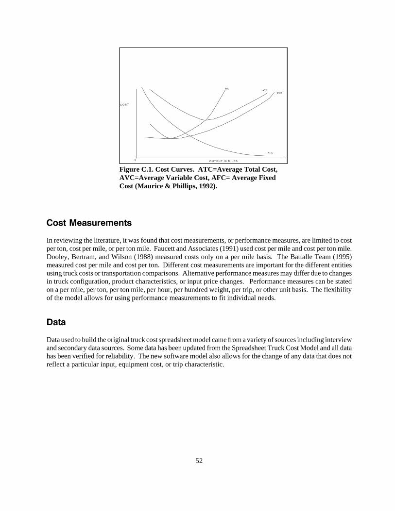
52

M CAT C

AV C

A F C

O U T P U T IN M IL E S

C O S T

0

Figure C.1. Cost Curves. ATC=Average Total Cost,AVC=Average Variable Cost, AFC= Average FixedCost (Maurice & Phillips, 1992).

Cost Measurements

In reviewing the literature, it was found that cost measurements, or performance measures, are limited to costper ton, cost per mile, or per ton mile. Faucett and Associates (1991) used cost per mile and cost per ton mile.Dooley, Bertram, and Wilson (1988) measured costs only on a per mile basis. The Battalle Team (1995)measured cost per mile and cost per ton. Different cost measurements are important for the different entitiesusing truck costs or transportation comparisons. Alternative performance measures may differ due to changesin truck configuration, product characteristics, or input price changes. Performance measures can be statedon a per mile, per ton, per ton mile, per hour, per hundred weight, per trip, or other unit basis. The flexibilityof the model allows for using performance measurements to fit individual needs.

Data

Data used to build the original truck cost spreadsheet model came from a variety of sources including interviewand secondary data sources. Some data has been updated from the Spreadsheet Truck Cost Model and all datahas been verified for reliability. The new software model also allows for the change of any data that does notreflect a particular input, equipment cost, or trip characteristic.

53

Cost Summary

Factors affecting costs in the trucking industry include economies of size, economies of utilization, and themakeup of variable and fixed costs. Economies of size for small firms and owner/operators may be minimal,and the cost structure of owner/operators may vary somewhat from larger firms because management andoverhead costs may be low or negligible. Small firms or owner/operators may increase size by adding powerunits to take advantage of volume discounts. Utilization is the most important factor affectingowner/operators. High use lowers average fixed costs for the owner/operator. It would be expected that smallchanges in equipment use would have a large impact on costs for the owner/operator.