Turbulence, Turbulent Mixing and GPU-Accelerated Computing

Turbulence, Turbulent Mixing and

GPU-Accelerated Computing on TITAN

P.K. Yeung (and Matthew P. Clay)Georgia Institute of TechnologyE-mail: [email protected]

Part 1: The Science

OLCF Users Meeting, Oak Ridge, May 15, 2018

Yeung & Clay, Part 1 Turbulence Aug 2017 1/18

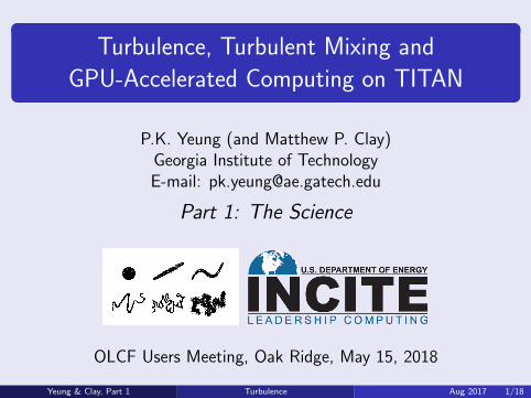
The Nature of Turbulence

Disorderly fluctuations in time and three-dimensional space— multi-scale, nonlinear, stochastic; interdisciplinary— crucial agent of transport, mixing and dispersion

(Sources: Wikipedia and Google search)

R. Feynman: “The Last Unsolved Problem of Classical Physics”

Also a Grand Challenge problem for high-performance computing


Introduction: Turbulent Mixing

Mixing: inter-mingling of entities of different properties ina fluid flow, with reduction of non-uniformity

Between different chemical species, clean vs polluted air

Between warm and cold fluids, fresh and salty water

May or may not affect the fluid motion itself

If not, called a “passive scalar” in fluid dynamics

Enhanced by turbulence, which carries “contaminants”around with fluid elements in disorderly motion

Large local gradients may form, subsequently smoothed out(“dissipated”) by molecular diffusion acting at the small scales

Overall results depend on intensity of turbulence, and magnitudeof molecular diffusivity versus kinematic viscosity of the fluid


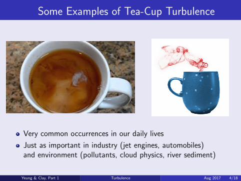
Some Examples of Tea-Cup Turbulence

Very common occurrences in our daily lives

Just as important in industry (jet engines, automobiles)and environment (pollutants, cloud physics, river sediment)


Evolution Equation for Passive Scalars

Advection-diffusion equation for scalar fluctuations in thepresence of a uniform mean gradient:

∂θ + u · ∇θ = −u · ∇〈Θ〉+ D∇2θ

(fluctuating) velocity field governed by Navier-Stokesequations for conservation of mass and momentum:

∇·u = 0

∂u/∂t + u·∇u = −∇(p/ρ) + ν∇2u + f

Simplified geometry, amenable to pseudo-spectral methods

Numerical forcing to maintain statistical stationarity in time


Resolution Requirements in DNS

Range of scales increases with the Reynolds number:

Domain size should be larger than largest scale (L)

Grid spacing should be comparable to smallest scale (η)

Number of grid points scale as (L/η)3 ∝ Rλ9/2 where Rλ is

Taylor-scale Reynolds number (based on intermediate scales)

More expensive if higher Reynolds number or better resolution isneeded or required (e.g. for study of intermittency)

Some notable references in the field:Kaneda et al. PoF 2003: 40963, on Earth Simulator

Yeung, Zhou & Sreenivasan PNAS 2015: 81923, on Blue Waters

Ishihara et al. PRF 2016: 122883, on K Computer


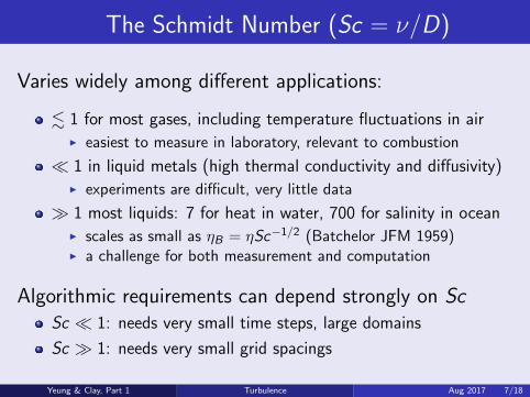
The Schmidt Number (Sc = ν/D)

Varies widely among different applications:

. 1 for most gases, including temperature fluctuations in airI easiest to measure in laboratory, relevant to combustion

1 in liquid metals (high thermal conductivity and diffusivity)I experiments are difficult, very little data

1 most liquids: 7 for heat in water, 700 for salinity in oceanI scales as small as ηB = ηSc−1/2 (Batchelor JFM 1959)I a challenge for both measurement and computation

Algorithmic requirements can depend strongly on ScSc 1: needs very small time steps, large domains

Sc 1: needs very small grid spacings


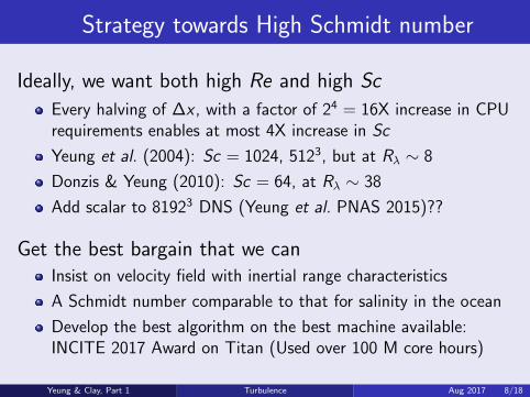
Strategy towards High Schmidt number

Ideally, we want both high Re and high Sc

Every halving of ∆x , with a factor of 24 = 16X increase in CPUrequirements enables at most 4X increase in Sc

Yeung et al. (2004): Sc = 1024, 5123, but at Rλ ∼ 8

Donzis & Yeung (2010): Sc = 64, at Rλ ∼ 38

Add scalar to 81923 DNS (Yeung et al. PNAS 2015)??

Get the best bargain that we canInsist on velocity field with inertial range characteristics

A Schmidt number comparable to that for salinity in the ocean

Develop the best algorithm on the best machine available:INCITE 2017 Award on Titan (Used over 100 M core hours)


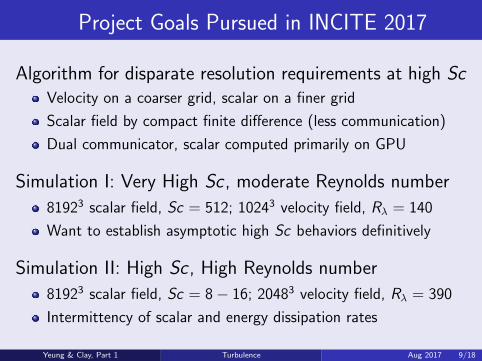
Project Goals Pursued in INCITE 2017

Algorithm for disparate resolution requirements at high ScVelocity on a coarser grid, scalar on a finer grid

Scalar field by compact finite difference (less communication)

Dual communicator, scalar computed primarily on GPU

Simulation I: Very High Sc , moderate Reynolds number

81923 scalar field, Sc = 512; 10243 velocity field, Rλ = 140

Want to establish asymptotic high Sc behaviors definitively

Simulation II: High Sc , High Reynolds number

81923 scalar field, Sc = 8− 16; 20483 velocity field, Rλ = 390

Intermittency of scalar and energy dissipation rates


Passive Scalars: Some Physical Questions

Note d〈θ2〉/dt = −2〈uθ〉·∇〈Θ〉 − 〈χ〉 where 〈χ〉 = 2D〈∇θ · ∇θ〉is the mean scalar dissipation rate

How are scalar fluctuations distributed among different scales?I Sc 1, in viscous-convective range: 1/η k 1/ηB

Theory of “local isotropy” in turbulence:I Do scalar gradients lose preferential orientation as Sc →∞?

Scalar dissipation fluctuations and intermittencyI How do “extreme events” of χ scale with Sc, and compare

with those of energy dissipation, at high Reynolds no.?


Batchelor Scaling of the Spectrum

Batchelor (JFM 1959) predicted Eθ(k) = CB〈χ〉(ν/〈ε〉)1/2k−1 inV-C range where kη 1 and kηB 1. A formula by Kraichnan(1968) also predicts behavior at kηB > 1 well

Batchelor suggested CB = 2, but most simulations give 5 ∼ 6

10−8

10−7

10−6

10−5

10−4

10−3

10−2

10−1

100

10−2 10−1 100 101 102

k −1

Increasing Sc

10−1

100

101

10−3 10−2 10−1 100

10−6

10−5

10−4

10−3

10−2

10−1

100

101

0 1 2 3 4

Eθ(k)

kη

kEθ(k)(〈ε〉/ν)1/2/〈χ

〉

kηB


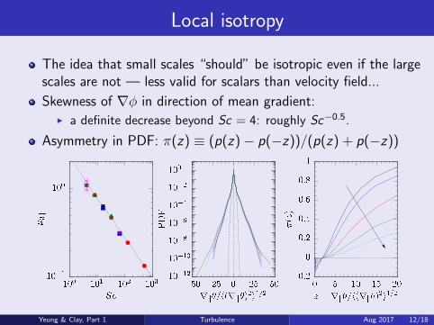
Local isotropy

The idea that small scales “should” be isotropic even if the largescales are not — less valid for scalars than velocity field...

Skewness of ∇φ in direction of mean gradient:I a definite decrease beyond Sc = 4: roughly Sc−0.5.

Asymmetry in PDF: π(z) ≡ (p(z)− p(−z))/(p(z) + p(−z))


Saturation of Intermittency

Flatness factor of scalar gradients which are highly non-Gaussian

Likelihood of samples of very large χ/〈χ〉 (hundreds, or higher)

Finite resolution can underestimate large gradients

Various Reynolds nos. and resolutions Rλ ∼ 140

1

ε

Sc

14

15

16

17

18

19

20

21

22

100 101 102 10310−1410−1210−1010−810−610−410−2100

0 100 200 300 400 500 600

µ4‖,µ4,⊥

Sc

PDF

χ/〈χ〉, ε/〈ε〉


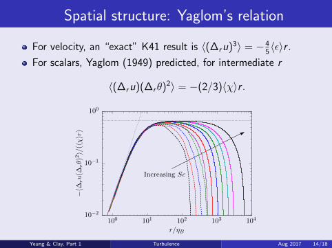
Spatial structure: Yaglom’s relation

For velocity, an “exact” K41 result is 〈(∆ru)3〉 = −45〈ε〉r .

For scalars, Yaglom (1949) predicted, for intermediate r

〈(∆ru)(∆rθ)2〉 = −(2/3)〈χ〉r .

10−2

10−1

100

100 101 102 103 104

Increasing Sc

−〈∆

ru

(∆rθ)

2〉/

(〈χ〉r

)

r/ηB


About “Extreme Events”

In turbulence, probability distribution of velocity and scalarfluctuations taken at a point are usually close Gaussian

But gradients in space are non-Gaussian, with localizedfluctuations of high intensity (spottiness in space)

Quadratic measures of such gradients are important:I ε ≡ 2νsijsij : energy dissipation rate (strain rates)I Ω ≡ νωiωi : enstrophy (vorticity squared)I χ ≡ 2D(∂θ/∂xi )(∂θ/∂xi ): scalar dissipation rate

Changes in shape and orientation of fluid elements, andoccurrence of large gradients (v. important in combustion)

Properties of ε taken pointwise or averaged over selected scalesizes are crucial in intermittency theory


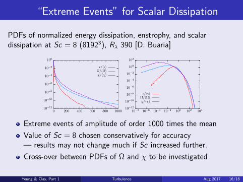
“Extreme Events” for Scalar Dissipation

PDFs of normalized energy dissipation, enstrophy, and scalardissipation at Sc = 8 (81923), Rλ 390 [D. Buaria]

10−12

10−10

10−8

10−6

10−4

10−2

100

0 200 400 600 800 1000

ǫ/〈ǫ〉Ω/〈Ω〉χ/〈χ〉

10−12

10−10

10−8

10−6

10−4

10−2

100

102

10−8 10−6 10−4 10−2 100 102 104

ǫ/〈ǫ〉Ω/〈Ω〉χ/〈χ〉

Extreme events of amplitude of order 1000 times the mean

Value of Sc = 8 chosen conservatively for accuracy— results may not change much if Sc increased further.

Cross-over between PDFs of Ω and χ to be investigated


Science Results: Summary and Further Questions

DNS of High Sc mixing up to Sc = 512, at Rλ ∼ 140

Viscous-convective scaling (between η and ηB = η/√Sc)

Reduction of anisotropy in the Sc 1 limit

Saturation of intermittency in small scales as Sc increases

Evidence of extreme events in scalar dissipation rate

Further questions and extensionsMore analyses: e.g to explain skewness of scalar gradientsvarying as Sc−1/2, and to obtain statistics of locally averaged χ

INCITE 2018 project on Titan:I Differential diffusion between Sc = 4 and 512I Active scalars in oceanic context: density of seawater depends

on both temperature (Sc = 7) and salinity (Sc = 700)


Some Publications

Gotoh, T. & PKY (2013) “Passive scalar transport: a computationalperspective”. in Ten Chapters in Turbulence, Cambridge UniversityPress, UK.

† Clay, M.P., Buaria, D., PKY & Gotoh, T. (2018) GPU accelerationof a petascale application for turbulent mixing at high Schmidtnumber using OpenMP 4.5.Comput. Phys. Commun., 228, 100-114.

Donzis, D.A., Sreenivasan, K.R. & PKY (2010) The Batchelorspectrum for mixing of passive scalars in isotropic turbulence.Flow, Turb. & Combust., 85, 549-566.

PKY, Zhai, X.M & Sreenivasan, K.R. (2015). Extreme events incomputational turbulence. PNAS, 112, 12633-12638.

†: INCITE publication


Documents

Turbulence, Turbulent Mixing and GPU-Accelerated Computing