Turbulent dissipation in a near-field river plume: A

Turbulent dissipation in a near-field river plume:

A comparison of control volume and microstructure observations with

a numerical model

Daniel G. MacDonald,1,2 Louis Goodman,1,2 and Robert D. Hetland3

Received 22 December 2006; revised 23 March 2007; accepted 10 May 2007; published 25 July 2007.

[1] Data collected from the near-field region (first several kilometers) of the MerrimackRiver plume are analyzed to provide estimates of turbulent kinetic energy (TKE)dissipation rates. Measurement techniques included a control volume methodincorporating density and velocity survey data, and direct dissipation rate measurementsby turbulence sensors mounted on an autonomous underwater vehicle (AUV). These twodistinct observational approaches are compared with TKE dissipation rates derived from ahighly resolved three-dimensional numerical model. In general, there is goodagreement between the three estimates of dissipation rate. Differences occurred in tworegions: (1) at the base of the plume, where plume density increased, and (2) in the verynear field of the plume, which is characterized by rapid acceleration and strongshoaling. Results suggest that there is a feedback between the turbulence and the plumeevolution with the result that the spreading rate of the plume is constrained. A scalingparameterization, relating turbulent dissipation rate to plume density and velocity, is alsoexamined. Immediately seaward of the front this parameterization appears to be consistentwith observed rates of dissipation, but progressing seaward, a modification to theparameterization may be necessary to account for plume spreading and deepening.

Citation: MacDonald, D. G., L. Goodman, and R. D. Hetland (2007), Turbulent dissipation in a near-field river plume: A comparison

of control volume and microstructure observations with a numerical model, J. Geophys. Res., 112, C07026,

doi:10.1029/2006JC004075.

1. Introduction

[2] The process of turbulence occurs over a wide range ofscales [e.g., Richardson, 1920], from the largest energycontaining scales, Lt, where energy from the mean flow istypically imparted to the turbulence, down to the Kolmo-gorov microscales, where turbulent energy is ultimatelydissipated into heat. Additionally, the impact of turbulencecan also be observed across scales much larger than theenergy containing scales, as the cumulative effect of mixingprocesses and the dissipation of energy originally derivedfrom the mean flow can result in significant alterations tothe density structure and momentum of the flow field. Assuch, it could be argued that turbulence is truly a phe-nomenon which is important across all scales of relevanceto a particular flow field.

[3] A key theoretical relationship in quantifying turbu-lence observations has been the usage of the steady stateturbulent kinetic energy budget equation [Gregg, 1987].However, up until recently the only technique which hasbeen typically employed in turbulence measurementsinvolved estimating one term of the TKE budget, thedissipation rate e. The standard technique to directly mea-sure e is the thrust probe sensor, originally developed bySiddon [1965] and initially employed in the ocean byOsborn [1974]. Typically this type of measurement is madeby a vertical profiler. Recently a number of alternativetechniques and platforms have been developed and usedto measure ocean turbulence. (For a review of such techni-ques, see Lueck et al. [2002]). One such platform which isparticularly useful for inferring e at very high resolution,both horizontally as well as vertically, is an AUV [Levine etal., 1997]. Recently, Goodman et al. [2006] have shownthat the thrust probe can be successfully mounted on such aplatform and produce very high quality measurements ofdissipation rate by employing a procedure which correctssensor vibration and vehicle motion effects arising from alldirections. The approach of using micro- and fine-scalesensors on an AUV is particularly useful for measuringturbulence and its local background processes in a field oflimited horizontal and vertical extent, such as in buoyantplumes and coastal fronts.

JOURNAL OF GEOPHYSICAL RESEARCH, VOL. 112, C07026, doi:10.1029/2006JC004075, 2007ClickHere

for

FullArticle

1Department of Estuarine and Ocean Sciences, School for MarineScience and Technology, University of Massachusetts-Dartmouth, NewBedford, Massachusetts, USA.

2University of Massachusetts School of Marine Sciences, Lowell,Massachusetts, USA.

3Department of Oceanography, Texas A&M University, CollegeStation, Texas, USA.

Copyright 2007 by the American Geophysical Union.0148-0227/07/2006JC004075$09.00

C07026 1 of 13

http://dx.doi.org/10.1029/2006JC004075

[4] Recently a technique has been developed [MacDonaldand Geyer, 2004; Chen and MacDonald, 2006] to obtain theother terms in the steady state TKE budget equation, namelythe buoyancy flux, B, and shear production, P, terms. Thetechnique involves using density and velocity transect datacollected at scales significantly larger than the energy con-taining scales [Kay and Jay, 2003; MacDonald and Geyer,2004;Chen andMacDonald, 2006]. A budget is formed oversome finite region of the flow field, or control volume,allowing the turbulent momentum (Reynolds stress) andbuoyancy fluxes to be inferred. Owing to the sensitivityrequired in identifying changes in flow structure, thesetechniques are best suited for high-energy environments,such as estuaries, and near-field river plumes, where veloc-ities are high and stratification is strong.[5] Numerical models can also be useful in understanding

the vertical and horizontal structure of turbulent fields [e.g.,Burchard and Baumert, 1995; Burchard et al., 2002].Traditional two equation turbulence models [e.g., Galperinet al., 1988; Rodi, 1987], as well as recent advances inturbulence modeling, such as the generic length-scale ap-proach [Umlauf and Burchard, 2003], have proven effectivein many cases. However, such second moment closureschemes are based on one-dimensional boundary layerphysics, and for energetic shear-stratified flows, the mod-eled turbulent field will be primarily dependent on thestability functional. Shear-stratified turbulence, particularlyin high-energy regimes, remains the major weakness ofsecond moment closure schemes, and it is unclear howaccurately these models can predict the magnitude of TKEdissipation rates and other important TKE parameters.[6] This paper describes measurements of TKE parame-

ters in the highly sheared outflow associated with a near-field river plume [e.g., Wright and Coleman, 1971]. Such aregion is characterized by supercritical flow extendingseveral kilometers seaward of a sharp bottom attached saltfront, typically located at the mouth of narrow estuariesduring high-discharge events (Figure 1). In this environ-ment, high stratification and strong velocity shears create avery active turbulent field, which results in rapid mixing ofthe discharging water with ambient ocean waters. Previousobservations have suggested that mixing is accomplished inthis environment primarily through the generation of

Kelvin-Helmholz instabilities [Geyer and Farmer, 1989;MacDonald and Geyer, 2004], resulting in energy con-taining scales of the turbulence of similar size to the

Ozmidov scale (LO ¼ eN�3ð Þ12, where N is the buoyancy

frequency).[7] In this manuscript, estimates of TKE quantities are

derived using the control volume technique described byMacDonald and Geyer [2004], and compared with directestimates of dissipation rates generated from microstructureinstrumentation mounted in a horizontal configuration on anAUV, and also with quantities generated from a numericalmodel of the near-field region. The results provide impor-tant insight into the evolution of the turbulent field acrossthe near-field plume region, as well as an opportunity forcomparison and validation of two relatively new measure-ment techniques, and model output. In theory, the funda-mental difference in scales associated with the measurementtechniques can also be exploited to further understand theheterogeneity of the turbulence field.[8] A description of the Merrimack River field study and

sampling efforts is described in section 2. Section 3 pro-vides a detailed description of the various measurementtechniques and the numerical model, and presents results.Comparisons between the observed and modeled turbulentquantities are discussed in section 4, along with implicationsfor the evolution of the near-field plume structure.

2. Merrimack River Field Site

[9] Field observations were conducted in the near-fieldregion of the Merrimack River plume on 21 May 2006. TheMerrimack River discharges into the Gulf of Maine approx-imately 6 km south of the New Hampshire–Massachusettsborder (see inset, Figure 2), with a watershed covering asignificant portion of the New Hampshire and northeastMassachusetts land area. The study occurred less than aweek after extensive flooding in the Merrimack River basinresulted in a discharge of nearly 3000 m3 s�1, the highest innearly 70 years. Discharge during the observation periodwas approximately 1260 m3 s�1. Discharges were measuredat USGS gauging station number 01100000 in Lowell,Massachusetts, 60 km upstream from the river mouth.

Figure 1. Cartoon of vertical structure of near-field plume region, showing velocity and densityprofiles. Shaded region represents ambient ocean water, while unshaded region represents river andplume water. Vertical mixing between the two water masses, which occurs along the interface, is notrepresented by the shading.

C07026 MACDONALD ET AL.: TURBULENCE IN A NEAR-FIELD PLUME

2 of 13

C07026

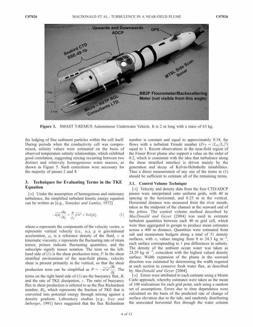
[10] Hydrographic data were collected from the Univer-sity of Massachusetts research vessel, the R/V Lucky Lady,using a towed conductivity temperature depth (CTD) unit(Ocean Sensors, OS200), and two RD Instruments 1200 kHzacoustic Doppler current profilers (ADCPs). One of theADCPs was mounted in a downward looking position offthe starboard side of the research vessel, the other in anupward looking orientation on an Acrobat (Sea Sciences,Inc.) tow body, which was towed approximately 3 m off thestarboard side of the vessel at a depth of approximately 4 m.The upward looking ADCP provided critical near surfacevelocity data which could not be resolved by the downwardlooking ADCP. The CTD sampled continuously at approx-imately 6 Hz, providing vertical resolution generally on theorder of 5 to 10 cm. The up and down motion of the tow-yosampling pattern also provided resolution in the horizontalof approximately 100 m. Both ADCP units were samplingat approximately 1 Hz, using 25 cm vertical bins. Inaddition, a REMUS AUV equipped with microstructureprobes (Figure 3) was deployed from a separate vessel.

[11] The location of five sampling transects are shown inFigure 2. Passes 1 through 4 were conducted with thesampling equipment aboard the R/V Lucky Lady. The trackof the REMUS AUV is also shown. Note that samplingpasses were repeated throughout the duration of the ebbtide, with the REMUS sampling period coinciding with pass4. The weather and sea state were calm, with a light offshorewind, and minimal swell.[12] The density and velocity structure of the near-field

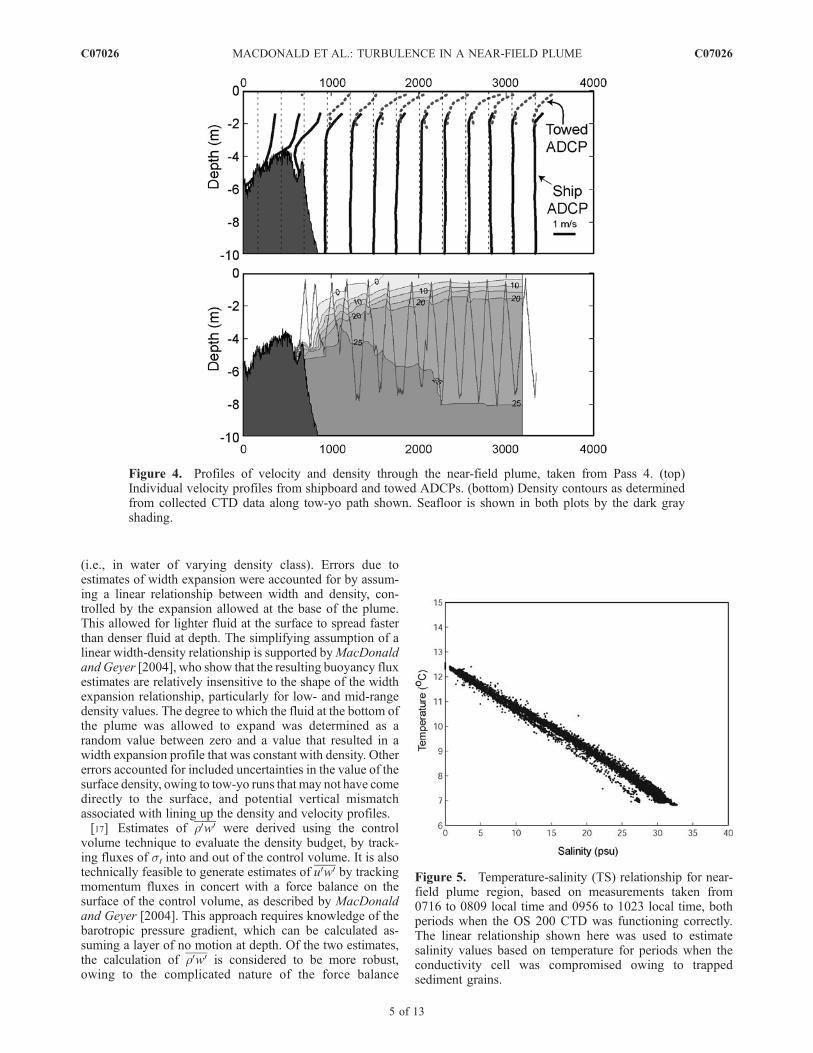
region is characterized by a rapidly thinning and mixingfresh water layer located seaward of a bottom attached saltfront (Figure 4). At the time of Pass 1, the salt front had notyet established itself at the estuary mouth, as ocean waterwas still present within the estuary. As the ebb progressed,the ocean water was expelled from the estuary, and some-time between Passes 1 and 2 a salt front was establishednear the bar located 400 to 600 m beyond the end of thejetties at the river mouth.[13] The discharging river water was also characterized

by a high coarse sediment load, which ultimately resulted inthe conductivity cell of the OS200 malfunctioning owing to

Figure 2. Location of sampling passes at mouth of Merrimack River. Passes 1 through 4 indicatelocations of CTD/ADCP transects performed from the R/V Lucky Lady. The line marked AUV indicatesthe location of the microstructure AUV run. Concentric circles indicate 1 km radii from the river mouth.Insets show the location of the Merrimack River mouth, near the Massachusetts–New Hampshire border,and the timing of the passes with respect to the tidal cycle on 21 May 2006. The AUV pass occurred atthe same time as Pass 4, as shown. Base map is from NOAA chart 13282 (December 1995).


3 of 13

C07026

the lodging of fine sediment particles within the cell itself.During periods when the conductivity cell was compro-mised, salinity values were estimated on the basis ofobserved temperature salinity relationships, which exhibitedgood correlation, suggesting mixing occurring between twodistinct and relatively homogeneous water masses, asshown in Figure 5. Such corrections were necessary forthe majority of passes 2 and 4.

3. Techniques for Evaluating Terms in the TKEEquation

[14] Under the assumption of homogenous and stationaryturbulence, the simplified turbulent kinetic energy equationcan be written as [e.g., Tennekes and Lumley, 1972]

�u0iu0j

@ui@xj

¼ g

ror0w0 þ 2ueijeij; ð1Þ

where u represents the components of the velocity vector, wrepresents vertical velocity (i.e., u3), g is gravitationalacceleration, ro is a reference density of the fluid, u iskinematic viscosity, e represents the fluctuating rate of straintensor, primes indicate fluctuating quantities, and thesubscripts signify tensor notation. The term on the left-hand side of (1) is the shear production term, P. In the shearstratified environment of the near-field plume, velocityshear is present primarily in the vertical, so that the shear

production term can be simplified as P = �u0w0 @u

@z. The

terms on the right hand side of (1) are the buoyancy flux, B,and the rate of TKE dissipation, e. The ratio of buoyancyflux to shear production is referred to as the flux Richardsonnumber, Rif, which represents the fraction of TKE that isconverted into potential energy through mixing against adensity gradient. Laboratory studies [e.g., Ivey andImberger, 1991] have suggested that the flux Richardson

number is constant and equal to approximately 0.18, forflows with a turbulent Froude number (FrT ¼ LO=Ltð Þ

23)

equal to 1. Recent observations in the near-field region ofthe Fraser River plume also support a value on the order of0.2, which is consistent with the idea that turbulence alongthe shear stratified interface is driven mainly by thegeneration and decay of Kelvin-Helmholtz instabilities.Thus a direct measurement of any one of the terms in (1)should be sufficient to estimate all of the remaining terms.

3.1. Control Volume Technique

[15] Velocity and density data from the four CTD/ADCPpasses were interpolated onto uniform grids, with 40 mspacing in the horizontal, and 0.25 m in the vertical.Horizontal distance was measured from the river mouth,taken as the midpoint of the channel at the seaward end ofthe jetties. The control volume method described byMacDonald and Geyer [2004] was used to estimateturbulent quantities between each 40 m grid cell, whichwere then aggregated in groups to produce mean estimatesacross a 400 m distance. Quantities were estimated fromsalt and momentum budgets along a total of 31 densitysurfaces, with st values ranging from 0 to 24.3 kg m�3,each surface corresponding to 1 psu differences in salinity.The density of the ambient ocean water was taken as24.29 kg m�3, coincident with the highest valued densitysurface. Width expansion of the plume in the seawarddirection was estimated by determining the width requiredat each section to conserve fresh water flux, as describedby MacDonald and Geyer [2004].[16] Errors were attributed to each estimate using a Monte

Carlo approach, whereby estimates were taken as the meanof 100 realizations for each grid point, each using a randomset of assumptions. Errors due to time dependence werecalculated on the basis of the predicted rate of change ofsurface elevation due to the tide, and randomly distributingthe associated horizontal flux through the water column

Figure 3. SMAST T-REMUS Autonomous Underwater Vehicle. It is 2 m long with a mass of 63 kg.


4 of 13

C07026

(i.e., in water of varying density class). Errors due toestimates of width expansion were accounted for by assum-ing a linear relationship between width and density, con-trolled by the expansion allowed at the base of the plume.This allowed for lighter fluid at the surface to spread fasterthan denser fluid at depth. The simplifying assumption of alinear width-density relationship is supported byMacDonaldand Geyer [2004], who show that the resulting buoyancy fluxestimates are relatively insensitive to the shape of the widthexpansion relationship, particularly for low- and mid-rangedensity values. The degree to which the fluid at the bottom ofthe plume was allowed to expand was determined as arandom value between zero and a value that resulted in awidth expansion profile that was constant with density. Othererrors accounted for included uncertainties in the value of thesurface density, owing to tow-yo runs that may not have comedirectly to the surface, and potential vertical mismatchassociated with lining up the density and velocity profiles.[17] Estimates of r0w0 were derived using the control

volume technique to evaluate the density budget, by track-ing fluxes of st into and out of the control volume. It is alsotechnically feasible to generate estimates of u0w0 by trackingmomentum fluxes in concert with a force balance on thesurface of the control volume, as described by MacDonaldand Geyer [2004]. This approach requires knowledge of thebarotropic pressure gradient, which can be calculated as-suming a layer of no motion at depth. Of the two estimates,the calculation of r0w0 is considered to be more robust,owing to the complicated nature of the force balance

Figure 4. Profiles of velocity and density through the near-field plume, taken from Pass 4. (top)Individual velocity profiles from shipboard and towed ADCPs. (bottom) Density contours as determinedfrom collected CTD data along tow-yo path shown. Seafloor is shown in both plots by the dark grayshading.

Figure 5. Temperature-salinity (TS) relationship for near-field plume region, based on measurements taken from0716 to 0809 local time and 0956 to 1023 local time, bothperiods when the OS 200 CTD was functioning correctly.The linear relationship shown here was used to estimatesalinity values based on temperature for periods when theconductivity cell was compromised owing to trappedsediment grains.


5 of 13

C07026

required to accurately constrain the u0w0 estimate. As such,only the r0w0 results are presented here, although bothestimates show qualitatively similar trends.[18] This technique allowed for the two dimensional

structure of the Reynolds density flux term, leading directlyto estimates of B, to be generated, providing a frameworkfor understanding the evolution of the turbulent field acrossthe first several kilometers of the near-field region. This is asignificant advancement over the results presented byMacDonald and Geyer [2004], which provided verticalprofiles at only one location within the near-field plume.[19] Contours and representative vertical profiles of

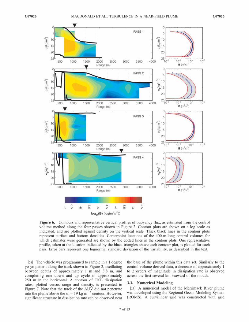
buoyancy flux, associated with passes 1 through 4, areshown in Figure 6. Note that these data are presented withrespect to density, and not depth. Bold black lines in eachcontour plot represent density of the surface and bottomwaters. Note the general trend of decreasing mixing awayfrom the river mouth, with buoyancy flux decreasing bymore than an order of magnitude in the first few kilometersseaward of the river mouth. Vertical profiles take a roughlyparabolic shape peaking in intensity at midrange densityvalues, and decaying toward zero at the surface and oceandensity contours.[20] The fact that turbulent quantities must decay to zero at

the plume boundaries is a critical constraint of the calculationtechnique. By definition, a turbulent process is one thatresults in no net transport of fluid. For example, followingthe Reynolds averaging technique (i.e., rw ¼ r0w0 þ r w ),all net transport of fluid on the right hand side is accom-plished by the advective term, r w , while the r0w0 termrepresents the transport of density accomplished onlythrough a compensating exchange of higher and lowerdensity fluids. Therefore focusing on the ocean densitycontour, which serves as the bounding surface separatingplume waters from an ocean assumed to be of uniformdensity, any turbulent transport of ambient ocean waterupward through that surface would have to be compensatedby an equal amount of plume water mixed downward,ultimately resulting in a displacement of the ocean densitycontour in the downward direction. Thus there can be noturbulent transport across the bottom boundary of theplume. There is, however, a significant upward directedadvective transport [see MacDonald and Geyer, 2004] ofambient ocean water across the bottom boundary of theplume, resulting in an upwelling which is necessary tosatisfy mass conservation and to feed all of the turbulentmixing processes occurring higher in the water column.

3.2. Turbulence AUV

[21] Direct values of the TKE dissipation rate wereobtained by using the SMAST AUV, T-REMUS vehicle.T-REMUS is a custom designed, extended REMUS, 1.9 min length with a mass of 63 kg. Mounted forward on thevehicle (see Figure 3) is the Micro ASTP developed byRGL Consultants (now Rockland Scientific International)of Victoria, BC. The Micro ASTP turbulence packageconsists of two orthogonal thrust probes, two FP07 fastresponse thermistors, three orthogonal accelerometersand a fast response pressure sensor. Also containedon the T-REMUS vehicle are an upward and downwardlooking 1.2 MHz ADCP, a FASTCAT CTD, a Wet Labs

BB2F Combination Spectral Backscattering Meter/Chloro-phyll Fluorometer, and a variety of ‘‘hotel’’ sensors mea-suring pitch, roll, yaw, and many other internal dynamicalcharacteristics of the T-REMUS vehicle. This suite ofsensors allows quantification of the key dynamical andkinematical turbulent and fine-scale physical processes.The turbulent and fine-scale parameters which can beestimated from the data collected by the T-REMUS include:the turbulent dissipation rate, fine-scale velocity shearand fine-scale stratification [see Levine and Lueck, 1999;Goodman et al., 2006].[22] Turbulent dissipation rate e is estimated by calculating

e ¼ 15

4

�@v

@xþ @w

@x

�; ð2Þ

where x is the along track direction, and v and w are thecross-track and vertical velocity components, respectively.Correction for vehicle motion and sensor vibration isperformed by coherently subtracting the three componentsof acceleration using a Weiner function filter (R. Lueck,personal communication, 2006) on the two components ofshear in equation (2). An analogous procedure for spectralcorrection is given by Goodman et al. [2006]. Equation (2)involves the assumption of isotropy at the smallest(Kolmogorov) scales of motion. Yamazaki and Osborn[1993] have shown that this assumption is valid for a value

ofe

nN2> 100.

[23] Dissipation rate was calculated by averaging the twoshear terms of (2) over 5 meters horizontally, whichtypically corresponded to 10 centimeters vertically. Therange of wave numbers making the dominant (90%) con-tribution to the dissipation rate is expected to be near thepeak in the shear spectra which is of order 0.1 times theKolmogorov wave number [Lueck et al., 2002]. For ourdata this peak occurs between 10 to 20 cyc/m (or 5 cm to10 cm length scale). Using an average over 5 meters in thehorizontal yields an effective number of degrees of freedomof order 20. (The peak in the shear spectra tended to occur atwave numbers > 20 cyc/m for e > 10�7 m2 s�3.) Shearspectra corresponding to e > 10�7 m2 s�3 had reasonableuniversal Nasmyth [1970] spectra with the v and w sheartending to be the same magnitude. Thus for this data set weestimate that noise levels were sufficiently low to trustdissipation rate values e > 10�7 m2 s�3 within calculatederror bounds. We calculated 90% error bounds by subsam-pling the data over a 0.4 m horizontal range (shear probedata being sampled at 500 Hz and the shear varianceaveraged over 200 points) and forming a histogram (pdf)of the subsampled e values using (2). The resulting rawvalues of e tended to follow a log normal distribution[Gregg, 1987], as expected. For dissipation rate values

e > 10�7 m2 s�3, approximately 70% had values ofe

nN2>

20, a boundary where active turbulence is expected to occur

[Itswiere et al., 1993]. For this range ofe

nN2values the

assumption of isotropy should lead to errors no greater than40% [Yamazaki and Osborn, 1990, 1993], which is typicallyof the same order or less than the error estimates describedabove.


6 of 13

C07026

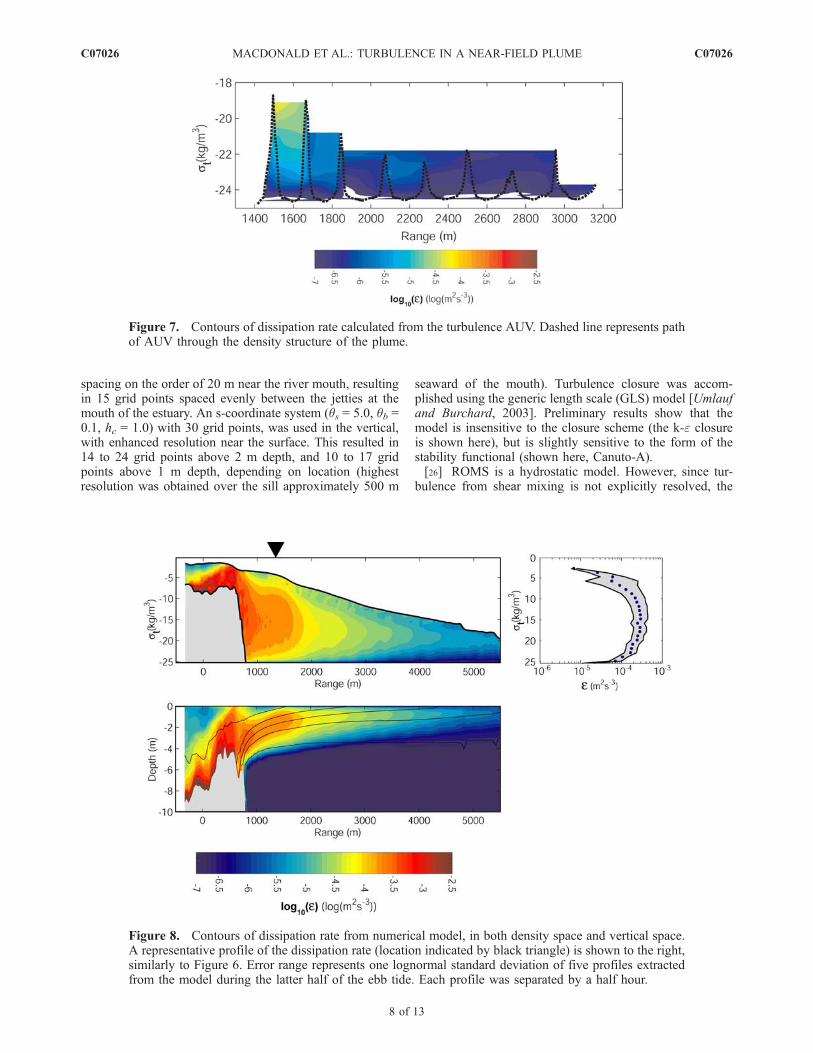
[24] The vehicle was programmed to sample in a 1 degreeyo-yo pattern along the track shown in Figure 2, oscillatingbetween depths of approximately 1 m and 3.8 m, andcompleting one down and up cycle in approximately250 m in the horizontal. A contour of TKE dissipationrates, plotted versus range and density, is presented inFigure 7. Note that the track of the AUV did not penetrateinto the plume above the st = 19 kg m�3 contour. However,significant structure in dissipation rate can be observed near

the base of the plume within this data set. Similarly to thecontrol volume derived data, a decrease of approximately 1to 2 orders of magnitude in dissipation rate is observedacross the first several km seaward of the mouth.

3.3. Numerical Modeling

[25] A numerical model of the Merrimack River plumewas developed using the Regional Ocean Modeling System(ROMS). A curvilinear grid was constructed with grid

Figure 6. Contours and representative vertical profiles of buoyancy flux, as estimated from the controlvolume method along the four passes shown in Figure 2. Contour plots are shown on a log scale asindicated, and are plotted against density on the vertical scale. Thick black lines in the contour plotsrepresent surface and bottom densities. Centerpoint locations of the 400-m-long control volumes forwhich estimates were generated are shown by the dotted lines in the contour plots. One representativeprofile, taken at the location indicated by the black triangles above each contour plot, is plotted for eachpass. Error bars represent one lognormal standard deviation of the variability, as described in the text.


7 of 13

C07026

spacing on the order of 20 m near the river mouth, resultingin 15 grid points spaced evenly between the jetties at themouth of the estuary. An s-coordinate system (qs = 5.0, qb =0.1, hc = 1.0) with 30 grid points, was used in the vertical,with enhanced resolution near the surface. This resulted in14 to 24 grid points above 2 m depth, and 10 to 17 gridpoints above 1 m depth, depending on location (highestresolution was obtained over the sill approximately 500 m

seaward of the mouth). Turbulence closure was accom-plished using the generic length scale (GLS) model [Umlaufand Burchard, 2003]. Preliminary results show that themodel is insensitive to the closure scheme (the k-e closureis shown here), but is slightly sensitive to the form of thestability functional (shown here, Canuto-A).[26] ROMS is a hydrostatic model. However, since tur-

bulence from shear mixing is not explicitly resolved, the

Figure 7. Contours of dissipation rate calculated from the turbulence AUV. Dashed line represents pathof AUV through the density structure of the plume.

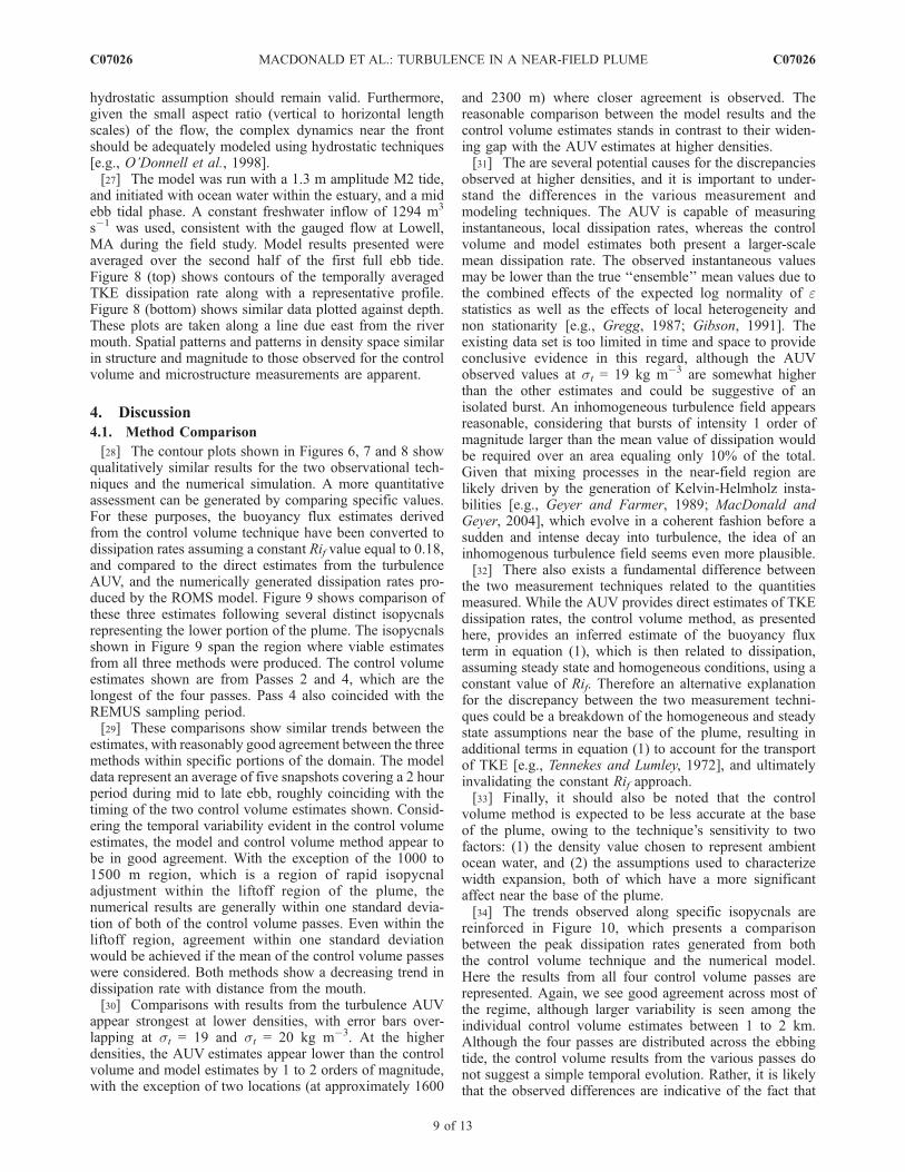
Figure 8. Contours of dissipation rate from numerical model, in both density space and vertical space.A representative profile of the dissipation rate (location indicated by black triangle) is shown to the right,similarly to Figure 6. Error range represents one lognormal standard deviation of five profiles extractedfrom the model during the latter half of the ebb tide. Each profile was separated by a half hour.


8 of 13

C07026

hydrostatic assumption should remain valid. Furthermore,given the small aspect ratio (vertical to horizontal lengthscales) of the flow, the complex dynamics near the frontshould be adequately modeled using hydrostatic techniques[e.g., O’Donnell et al., 1998].[27] The model was run with a 1.3 m amplitude M2 tide,

and initiated with ocean water within the estuary, and a midebb tidal phase. A constant freshwater inflow of 1294 m3

s�1 was used, consistent with the gauged flow at Lowell,MA during the field study. Model results presented wereaveraged over the second half of the first full ebb tide.Figure 8 (top) shows contours of the temporally averagedTKE dissipation rate along with a representative profile.Figure 8 (bottom) shows similar data plotted against depth.These plots are taken along a line due east from the rivermouth. Spatial patterns and patterns in density space similarin structure and magnitude to those observed for the controlvolume and microstructure measurements are apparent.

4. Discussion

4.1. Method Comparison

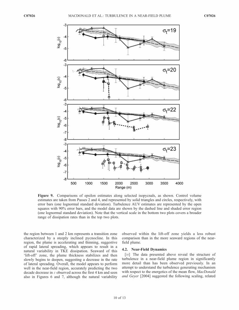
[28] The contour plots shown in Figures 6, 7 and 8 showqualitatively similar results for the two observational tech-niques and the numerical simulation. A more quantitativeassessment can be generated by comparing specific values.For these purposes, the buoyancy flux estimates derivedfrom the control volume technique have been converted todissipation rates assuming a constant Rif value equal to 0.18,and compared to the direct estimates from the turbulenceAUV, and the numerically generated dissipation rates pro-duced by the ROMS model. Figure 9 shows comparison ofthese three estimates following several distinct isopycnalsrepresenting the lower portion of the plume. The isopycnalsshown in Figure 9 span the region where viable estimatesfrom all three methods were produced. The control volumeestimates shown are from Passes 2 and 4, which are thelongest of the four passes. Pass 4 also coincided with theREMUS sampling period.[29] These comparisons show similar trends between the

estimates, with reasonably good agreement between the threemethods within specific portions of the domain. The modeldata represent an average of five snapshots covering a 2 hourperiod during mid to late ebb, roughly coinciding with thetiming of the two control volume estimates shown. Consid-ering the temporal variability evident in the control volumeestimates, the model and control volume method appear tobe in good agreement. With the exception of the 1000 to1500 m region, which is a region of rapid isopycnaladjustment within the liftoff region of the plume, thenumerical results are generally within one standard devia-tion of both of the control volume passes. Even within theliftoff region, agreement within one standard deviationwould be achieved if the mean of the control volume passeswere considered. Both methods show a decreasing trend indissipation rate with distance from the mouth.[30] Comparisons with results from the turbulence AUV

appear strongest at lower densities, with error bars over-lapping at st = 19 and st = 20 kg m�3. At the higherdensities, the AUV estimates appear lower than the controlvolume and model estimates by 1 to 2 orders of magnitude,with the exception of two locations (at approximately 1600

and 2300 m) where closer agreement is observed. Thereasonable comparison between the model results and thecontrol volume estimates stands in contrast to their widen-ing gap with the AUV estimates at higher densities.[31] The are several potential causes for the discrepancies

observed at higher densities, and it is important to under-stand the differences in the various measurement andmodeling techniques. The AUV is capable of measuringinstantaneous, local dissipation rates, whereas the controlvolume and model estimates both present a larger-scalemean dissipation rate. The observed instantaneous valuesmay be lower than the true ‘‘ensemble’’ mean values due tothe combined effects of the expected log normality of estatistics as well as the effects of local heterogeneity andnon stationarity [e.g., Gregg, 1987; Gibson, 1991]. Theexisting data set is too limited in time and space to provideconclusive evidence in this regard, although the AUVobserved values at st = 19 kg m�3 are somewhat higherthan the other estimates and could be suggestive of anisolated burst. An inhomogeneous turbulence field appearsreasonable, considering that bursts of intensity 1 order ofmagnitude larger than the mean value of dissipation wouldbe required over an area equaling only 10% of the total.Given that mixing processes in the near-field region arelikely driven by the generation of Kelvin-Helmholz insta-bilities [e.g., Geyer and Farmer, 1989; MacDonald andGeyer, 2004], which evolve in a coherent fashion before asudden and intense decay into turbulence, the idea of aninhomogenous turbulence field seems even more plausible.[32] There also exists a fundamental difference between

the two measurement techniques related to the quantitiesmeasured. While the AUV provides direct estimates of TKEdissipation rates, the control volume method, as presentedhere, provides an inferred estimate of the buoyancy fluxterm in equation (1), which is then related to dissipation,assuming steady state and homogeneous conditions, using aconstant value of Rif. Therefore an alternative explanationfor the discrepancy between the two measurement techni-ques could be a breakdown of the homogeneous and steadystate assumptions near the base of the plume, resulting inadditional terms in equation (1) to account for the transportof TKE [e.g., Tennekes and Lumley, 1972], and ultimatelyinvalidating the constant Rif approach.[33] Finally, it should also be noted that the control

volume method is expected to be less accurate at the baseof the plume, owing to the technique’s sensitivity to twofactors: (1) the density value chosen to represent ambientocean water, and (2) the assumptions used to characterizewidth expansion, both of which have a more significantaffect near the base of the plume.[34] The trends observed along specific isopycnals are

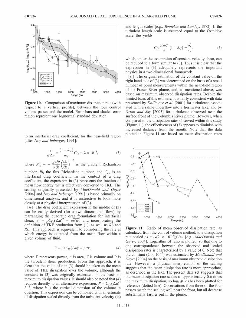
reinforced in Figure 10, which presents a comparisonbetween the peak dissipation rates generated from boththe control volume technique and the numerical model.Here the results from all four control volume passes arerepresented. Again, we see good agreement across most ofthe regime, although larger variability is seen among theindividual control volume estimates between 1 to 2 km.Although the four passes are distributed across the ebbingtide, the control volume results from the various passes donot suggest a simple temporal evolution. Rather, it is likelythat the observed differences are indicative of the fact that


9 of 13

C07026

the region between 1 and 2 km represents a transition zonecharacterized by a steeply inclined pycnocline. In thisregion, the plume is accelerating and thinning, suggestiveof rapid lateral spreading, which appears to result in anatural variability in TKE dissipation. Seaward of this‘lift-off’ zone, the plume thickness stabilizes and thenslowly begins to deepen, suggesting a decrease in the rateof lateral spreading. Overall, the model appears to performwell in the near-field region, accurately predicting the twodecade decrease in e observed across the first 4 km and seenalso in Figures 6 and 7, although the natural variability

observed within the lift-off zone yields a less robustcomparison than in the more seaward regions of the near-field plume.

4.2. Near-Field Dynamics

[35] The data presented above reveal the structure ofturbulence in a near-field plume region in significantlymore detail than has been observed previously. In anattempt to understand the turbulence generating mechanismwith respect to the energetics of the mean flow, MacDonaldand Geyer [2004] suggested the following scaling, related

Figure 9. Comparisons of epsilon estimates along selected isopycnals, as shown. Control volumeestimates are taken from Passes 2 and 4, and represented by solid triangles and circles, respectively, witherror bars (one lognormal standard deviation). Turbulence AUV estimates are represented by the opensquares with 90% error bars, and the model data are shown by the dashed line and shaded error region(one lognormal standard deviation). Note that the vertical scale in the bottom two plots covers a broaderrange of dissipation rates than in the top two plots.


10 of 13

C07026

to an interfacial drag coefficient, for the near-field region[after Ivey and Imberger, 1991]:

eg0Du

¼1� Rif� �

RigCDi � 2� 10�3; ð3Þ

where Rig = � g

r@r@z

@u

@z

� ��2

is the gradient Richardson

number, Rif the flux Richardson number, and CDi is aninterfacial drag coefficient. In the context of a dragcoefficient, the expression in (3) represents the fraction ofmean flow energy that is effectively converted to TKE. Thescaling originally presented by MacDonald and Geyer[2004] and Ivey and Imberger [1991] is based primarily ondimensional analysis, and it is instructive to look moreclosely at a physical interpretation of (3).[36] The drag coefficient expression in the middle of (3)

can be easily derived (for a two-dimensional flow) byrearranging the quadratic drag formulation for interfacialshear, ti = rCDi(Du)2 = ru0w0, and incorporating thedefinition of TKE production from (1), as well as Rif andRig. This approach is equivalent to considering the rate atwhich energy is extracted from the mean flow within agiven volume of fluid,

G ¼ rACDi Duð Þ3¼ rPV; ð4Þ

where G represents power, A is area, V is volume and P isthe turbulent shear production. From this approach, it isclear that the value of e in (3) should be taken as the meanvalue of TKE dissipation over the volume, although theconstant in (3) was originally estimated on the basis ofmaximum dissipation values. It should also be noted that (4)reduces directly to an alternative expression, P = CDi(Du)3

h�1, where h is the vertical dimension of the volume inquestion. This expression can be combined with an estimateof dissipation scaled directly from the turbulent velocity (ut)

and length scales [e.g., Tennekes and Lumley, 1972]. If theturbulent length scale is assumed equal to the Ozmidovscale, this yields

CDi

Duð Þ3

h1� Rif� �

¼ u3tLo

; ð5Þ

which, under the assumption of constant velocity shear, canbe reduced to a form similar to (3). Thus it is clear that theexpression in (3) adequately represents the importantphysics in a two-dimensional framework.[37] The original estimation of the constant value on the

right hand side of (3) was determined on the basis of a smallnumber of point measurements within the near-field regionof the Fraser River plume, and, as mentioned above, wasbased on maximum observed dissipation rates. Despite thelimited basis of this estimate, it is fairly consistent with datapresented by Dallimore et al. [2001] for turbulence associ-ated with a saline underflow into a freshwater lake, and byOrton and Jay [2005] for turbulence observed near thesurface front of the Columbia River plume. However, whencompared to the dissipation rates observed within this study(Figure 11), the effectiveness of (3) appears to diminish withincreased distance from the mouth. Note that the dataplotted in Figure 11 are based on mean dissipation rates

Figure 10. Comparison of maximum dissipation rate (withrespect to a vertical profile), between the four controlvolume passes and the model. Error bars and shaded errorregion represent one lognormal standard deviation.

Figure 11. Ratio of mean observed dissipation rate, ascalculated from the control volume method, to a dissipationrate scaled as e �(2 � 10�3)g0Du [e.g., MacDonald andGeyer, 2004]. Logarithm of ratio is plotted, so that one toone correspondence between the observed and scaleddissipation rates is characterized by a value of 0. Note thatthe constant (2 � 10�3) was estimated by MacDonald andGeyer [2004] on the basis of maximum observed dissipationrate. However, a physical interpretation of the scalingsuggests that the mean dissipation rate is more appropriate,as described in the text. The present data set suggests thatthe mean dissipation rate scales as approximately 0.6 timesthe maximum dissipation, so log10(0.6) has been plotted forreference (dotted line). Observations from three of the fourpasses match the scaling well near the front, but all decreasesubstantially farther out in the plume.


11 of 13

C07026

observed across the entire plume depth, and that the dottedline represents an approximate scaling factor between themean and maximum dissipation values. The data plotted inFigure 11 suggest that the ratio (e=g0Du) may not be constant,as suggested in (3).[38] The near-field plume is a complicated region, with

the flow field undergoing rapid adjustments, not only in thevertical, as shown in Figure 4, but also in the horizontal [seeHetland, 2005]. In the lift-off region, rapid shoaling of theplume can cause significant acceleration. However, hori-zontal divergence of streamlines within the plume, drivenby lateral pressure gradients resulting from the densitydifference between the plume waters and ambient oceanwaters, can temper the shoaling-driven acceleration. Thepresence of active turbulence not only produces a drag forceon the plume waters, directly decelerating the advancingplume, but may also play a role in modifying the rate ofwidth expansion due to a direct influence on the lateralpressure gradient.[39] It is clear that both vertical and lateral effects are

important to the evolution of the plume and the turbulentfield. The gradient Richardson number characterizes manyof the vertical influences, and its importance to the value ofthe dissipation rate is apparent from the expression in (3),and the physical discussion presented above. However,physics associated with the lateral dynamics are not explic-itly included in (3), which was derived within a two-dimensional framework. A Buckingham-Pi scaling analysisof the three-dimensional near-field plume problem suggeststhat there should be three independent nondimensional

parameters, which can be accounted for by the ratioe

g0Du,

the gradient Richardson number, Rig, and a third parameter

representing the rate of width expansion (i.e.,@b

@x). Given

that the value of Rig is relatively constant across the near-field region, it is likely that the rate of width expansion may

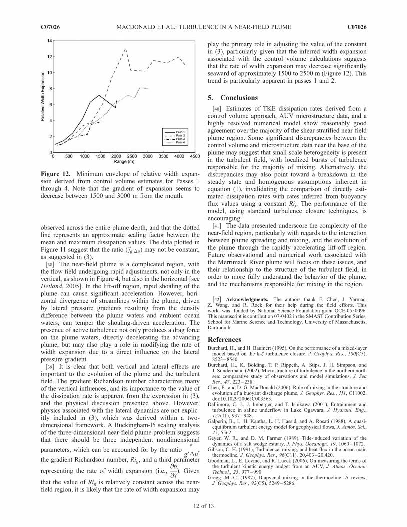
play the primary role in adjusting the value of the constantin (3), particularly given that the inferred width expansionassociated with the control volume calculations suggeststhat the rate of width expansion may decrease significantlyseaward of approximately 1500 to 2500 m (Figure 12). Thistrend is particularly apparent in passes 1 and 2.

5. Conclusions

[40] Estimates of TKE dissipation rates derived from acontrol volume approach, AUV microstructure data, and ahighly resolved numerical model show reasonably goodagreement over the majority of the shear stratified near-fieldplume region. Some significant discrepancies between thecontrol volume and microstructure data near the base of theplume may suggest that small-scale heterogeneity is presentin the turbulent field, with localized bursts of turbulenceresponsible for the majority of mixing. Alternatively, thediscrepancies may also point toward a breakdown in thesteady state and homogenous assumptions inherent inequation (1), invalidating the comparison of directly esti-mated dissipation rates with rates inferred from buoyancyflux values using a constant Rif. The performance of themodel, using standard turbulence closure techniques, isencouraging.[41] The data presented underscore the complexity of the

near-field region, particularly with regards to the interactionbetween plume spreading and mixing, and the evolution ofthe plume through the rapidly accelerating lift-off region.Future observational and numerical work associated withthe Merrimack River plume will focus on these issues, andtheir relationship to the structure of the turbulent field, inorder to more fully understand the behavior of the plume,and the mechanisms responsible for mixing in the region.

[42] Acknowledgments. The authors thank F. Chen, J. Yarmac,Z. Wang, and R. Rock for their help during the field efforts. Thiswork was funded by National Science Foundation grant OCE-0550096.This manuscript is contribution 07-0402 in the SMAST Contribution Series,School for Marine Science and Technology, University of Massachusetts,Dartmouth.

ReferencesBurchard, H., and H. Baumert (1995), On the performance of a mixed-layermodel based on the k-e turbulence closure, J. Geophys. Res., 100(C5),8523–8540.

Burchard, H., K. Bolding, T. P. Rippeth, A. Stips, J. H. Simpson, andJ. Sundermann (2002), Microstructure of turbulence in the northern northsea: comparative study of observations and model simulations, J. SeaRes., 47, 223–238.

Chen, F., and D. G. MacDonald (2006), Role of mixing in the structure andevolution of a buoyant discharge plume, J. Geophys. Res., 111, C11002,doi:10.1029/2006JC003563.

Dallimore, C. J., J. Imberger, and T. Ishikawa (2001), Entrainment andturbulence in saline underflow in Lake Ogawara, J. Hydraul. Eng.,127(11), 937–948.

Galperin, B., L. H. Kantha, L. H. Hassid, and A. Rosati (1988), A quasi-equilibrium turbulent energy model for geophysical flows, J. Atmos. Sci.,45, 5562.

Geyer, W. R., and D. M. Farmer (1989), Tide-induced variation of thedynamics of a salt wedge estuary, J. Phys. Oceanogr., 19, 1060–1072.

Gibson, C. H. (1991), Turbulence, mixing, and heat flux in the ocean mainthermocline, J. Geophys. Res., 96(C11), 20,403–20,420.

Goodman, L., E. Levine, and R. Lueck (2006), On measuring the terms ofthe turbulent kinetic energy budget from an AUV, J. Atmos. OceanicTechnol., 23, 977–990.

Gregg, M. C. (1987), Diapycnal mixing in the thermocline: A review,J. Geophys. Res., 92(C5), 5249–5286.

Figure 12. Minimum envelope of relative width expan-sion derived from control volume estimates for Passes 1through 4. Note that the gradient of expansion seems todecrease between 1500 and 3000 m from the mouth.


12 of 13

C07026

Hetland, R. D. (2005), Relating river plume structure to vertical mixing,J. Phys. Oceanogr., 35, 1667–1688.

Itswiere, E. C., J. R. Koseff, D. A. Bruggs, and J. H. Ferzinger (1993),Turbulence in stratified shear flows: Implication for interpreting shear-induced mixing in the ocean, J. Phys. Oceanogr., 23, 1508–1522.

Ivey, G. N., and J. Imberger (1991), On the nature of turbulence in astratified fluid. Part I: The energetics of mixing, J. Phys. Oceanogr.,21, 650–658.

Kay, D. J., and D. A. Jay (2003), Interfacial mixing in a highly stratifiedestuary: 1. A ‘‘method of constrained differences’’ approach for the de-termination of the momentum and mass balances and the energy of mix-ing, J. Geophys. Res., 108(C3), 3073, doi:10.1029/2000JC000253.

Levine, E. R., and R. G. Lueck (1999), Turbulence measurements from anautonomous underwater vehicle, J. Atmos. Oceanic Technol., 16, 1533–1544.

Levine, E. R., D. Connors, R. Shell, and R. Hanson (1997), Autonomousunderwater vehicle-based hydrographic sampling, J. Atmos. OceanicTechnol., 14, 1444–1454.

Lueck, R. G., F. Wolk, and H. Yamazaki (2002), Oceanic velocity turbu-lence measurements in the 20th century, J. Oceanogr., 58, 153–174.

MacDonald, D. G., and W. R. Geyer (2004), Turbulent energy productionand entrainment at a highly stratified estuarine front, J. Geophys. Res.,109, C05004, doi:10.1029/2003JC002094.

Nasmyth, P. W. (1970), Ocean turbulence, Ph.D. thesis, Univ. of B. C.,Vancouver, B. C., Canada.

O’Donnell, J., G. O. Marmorino, and C. L. Trump (1998), Convergence anddownwelling at a river plume front, J. Phys. Oceanogr., 28, 1481–1495.

Orton, P. M., and D. A. Jay (2005), Observations at the tidal plume front ofa high-volume river outflow, Geophys. Res. Lett., 32, L11605,doi:10.1029/2005GL022372.

Osborn, T. R. (1974), Vertical profiling of velocity microstructure, J. Phys.Oceanogr., 4, 109–115.

Richardson, L. F. (1920), The supply of energy from and to atmosphericeddies, Proc. R. Soc., Ser. A, 97, 354–373.

Rodi, W. (1987), Examples of calculation methods for flow and mixing instratified fluids, J. Geophys. Res., 92(C5), 5305–5328.

Siddon, T. F. (1965), A turbulence probe utilizing aerodynamic lift, Rev.Sci. Instrum., 42, 653–656.

Tennekes, H., and J. L. Lumley (1972), A First Course in Turbulence, MITPress, Cambridge, Mass.

Umlauf, L., and H. Burchard (2003), A generic length-scale equation forgeophysical turbulence models, J. Mar. Res., 61, 235–265.

Wright, L. D., and J. M. Coleman (1971), Effluent expansion and interfacialmixing in the presence of a salt wedge, Mississippi River Delta, J. Geo-phys Res., 76(36), 8649–8661.

Yamazaki, H., and T. Osborn (1990), Dissipation estimates for stratifiedturbulence, J. Geophys. Res., 95(C6), 9739–9744.

Yamazaki, H., and T. Osborn (1993), Erratum: ‘‘Dissipation Estimates ForStratified Turbulence’’ [Journal of Geophysical Research, 95, 9739–9744 (1990)], J. Geophys. Res., 98(C7), 12,605–12,606.

��L. Goodman and D. G. MacDonald, Department of Estuarine and Ocean

Sciences, School for Marine Science and Technology, University ofMassachusetts Dartmouth, 706 South Rodney French Boulevard, NewBedford, MA 02744-1221, USA. ([email protected])R. D. Hetland, Department of Oceanography, Texas A&M University,

College Station, TX 77843, USA.


13 of 13

C07026

Documents

Turbulent dissipation in a near-field river plume: A