NASA Technical Memorandum 89451

Reynolds-Stress and Dissipation Rate Budgets in a Turbulent Channel Flow N. N. Mansour J. Kim P. Moin, Ames Research Center, Moffett Field, California

December 1987

NASA National Aeronautics and Space Administration

Ames Research Center Moffett Field. California 94035

Reynolds-stress and dissipation rate budgets in a turbulent channel flow

N. N. Mansour, J. Kim and P. Moint NASA Ames Research Center, Moffett Field, CA 94035, USA

The budget.s for the Reynolds stresses and for the dissipation rate of the turbulence kinetic energy are computed using direct simulation data of a turbulent channel flow. The budget, data reveal that all the terms in the budget become important close to the wall. For inhomogeneous pressure boundary conditions, the pressure-strain term is split into a return term, a rapid term, and a Stokes term. The Stokes term is important. close to the wall. The rapid and return terms play different roles depending on the component of the term. A split of the velocity pressure-gradient term into a redist.ribut,ive t,erni and a diffusion term is proposed, which should be simpler to model. The budget dat,a is used to test existing closure models for the pressure-strain term, the dissipation rate, and the transport rate. In general, further work is needed to improve the models.

1. Introduction

The advancement of large-scale computers has led to the wide use of turbulence models to predict turbulent flows. At the 1980-81 AFOSR-HTTM-Stanford conference, phenomenological models of all categories (one-, two-, and Reynolds-stress-equations) were used to model various flows. The anticipated result, that transport models for the Reynolds-stress equations will outperform eddy-viscosity-type closures, did not happen. In fact, in simple flows, mixing-length models produced results as good or better than Reynolds-stress models. However, the same Reynolds-stress models were used in a variety of flows to simulate quantities that simpler models could not model. The possibility of using the same model with the same constants for a variety of flows is the niain motivation behind developing models at the Reynolds-stress level.

According to Lumley (1978), the history of “higher-order” modeling dates as far back as Kolmogorov (1942), who was the first to suggest the characterization of turbulence by its int,ensity and scale. Chou (1945 a) considered the full Reynolds-stress equations and the triple-correlation equations t,o close the averaged Navier-Stokes equation. He suggested that the use of equations up to third moments is sufficient to characterize turbulent flows and, wit,h simplifications, he predicted the mean velocity profile of a turbulent channel flow (Chou, 1945 b) which is the flow of interest in this work.

Rotta (1951a) developed closure models for the Reynolds-stress equations and ad- vanced models for the pressure-strain and the dissipation rate terms that, are the basis for several of the present, day models. In a followup paper, Rotta (1951 b) introduced an equation for the turbulence length scale and tested his models by simulating a turbulent channel flow. He found that the peak in the turbulence intensity could not be predicted

tAlso Department of Mechanical Engineering, Stanford University, Stanford, CA, USA

1

by his theory. Davydov (1959) proposed closures at the Reynolds-stress and the triple- correlation equations levels. Later, Davydov (1961) proposed closures for the equation of the dissipation rate of the turbulence kinetic energy ( c ) which are used by most present-day E-equations. Daly gL Harlow (1970) (hereafter referred to as DH) used various ideas to close the Reynolds-st.ress equations and used gradient-transport to model the turbulent diffusion terms. They added the scalar equation representing the trace of the dissipation rate tensor to the Reynolds-stress equations. They also computed the channel flow with mixed success in predicting the Reynolds-stresses. Launder, Reece, & Rodi (1975) (hereafter referred t>o as LRR) advanced closure forms to the Reynolds-stress equations that were tested for a variety of turbulent flows. Their models were developed for high Reynolds number flows. Hanjalii. & Launder (1976) (hereafter referred to as HL2) extended the model of LRR to simulate low-Reynolds-number turbulence and the near-wall region. HL2 computed the channel flow and found that their model underpredicts the peak in the turbulence kinetic energy by 30%. More recently, Shih & Lumley (1986) proposed closure forms to the pressure-strain terms that seem to hold promise but did not use the model to compute to the wall (wall functions were used in the near-wall region).

All of the work on turbulence modeling development uses indirect methods to test the various closure models. Because of the difficulty in measuring pressure and velocity with sufficient spatial accuracy, direct comparison of the closure models with experimental data has not been possible. Often, the adequacy of the model is judged by computing a flow with the model and by comparing the predicted mean velocity and Reynolds stresses with experimental data. With the advent of large-scale computers and new algorithm developments, direct simulations of turbulent flows are now possible at moderate Reynolds numbers. These simulations are being used to compute the terms in the budget of the Reynolds st,resses. It is then possible to test the closure models by direct comparison of the closure formula with the term being modeled.

A comprehensive testing of one point closure models using simulation data was carried out by Rogallo (1981) where he t3ested different pressure-strain models for homogeneous flows under mean strain and shear. Recently, direct simulations of simple inhomogeneous flows have been carried out by Kim, Moin & Moser (1987) (hereafter referred to as KMM), Moser 8L Moin (1984), and Spalart (1986a, 1986b). KMM computed the fully turbulent channel flow using two different grid resolutions (2 x lo6 and 4 x lo6 grid points) and found no dependency of the results on grid resolution. They compared their results with experimental data and were able to study the behavior of turbulence correlations near the wall. Although there exist some disagreements between experimental data and com- puted results, especially in the near wall region, the overall agreements were good. KMM attributed the differences to possible probe errors due to wall proximity. Moser 8t Moin computed a channel flow with mild streamwise curvature. They showed that the presence of the Gortler vortices contribute substantially to the shear stress. They also computed the terms in the budget of the Reynolds stresses. Spalart (1986a) computed boundary-layer flows with favorable pressure gradient and more recently (Spalart, 19868) computed tur- bulent boundary layers with zero pressure gradient up to Reo = 1410. These simulations were carried out at moderate Reynolds numbers and were used to compute the Reynolds

2

stresses and the terms in their budgets.

The objective of this work is to present the budget data for the Reynolds stresses and the budget data for the dissipation rate of the turbulence kinetic energy using the flow fields of KMM. These budgets are needed for model development because they will provide a direct means to evaluate closure models. The budget data for the dissipation rat e of the turbulence kinetic energy have eluded measurement techniques and will provide valuable guidelines for model developers and model testing. We will use these budgets to evaluate some existing algebraic models for the dissipation rate of the Reynolds stresses. Closure models for the budget of the dissipation rate of the turbulence kinetic energy will be evaluated. We will also compare with the data some existing models for the pressure- strain and the turbulent transport rate of the Reynolds stresses.

2. Channel data analyses

The use of direct simulation to compute turbulent flow fields will be restricted to simple flows for the forseeable future. The flows of engineering interest are simulated using the averaged Navier-St,okes equations in conjunction with closure models. With the advent of large computers, the trend will be towards using closures at the level of the budget, for the Reynolds dresses.

2.1. Reynolds stress budget

The transport equations for the Reynolds stresses are derived from the Navier-Stokes equations by ensemble averaging the equations, then deriving equations for the fluctuat- ing dresses and ensemble averaging these equations. For incompressible turbulent flow, the transport equations nondimensionalized with u$/v (the wall-shear velocity, u , = ,/=, and the kineiliatic viscosity, v) are given by

where o / D t = d / d t + i ! J k a / d Z k , and the terms on the right-hand side of the above equation are identified as follows:

Production rate

Dissipation rate

Turbulent transport rate

Viscous diffusion rate

Velocity pressure-gradient term

3

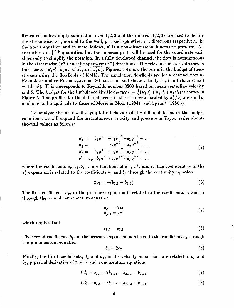
Repeated indices imply summation over 1,2,3 and the indices (1,2,3) are used to denote the streamwise, z+, normal to the wall, y+ , and spanwise, t+, directions respectively. In the above equation and in what follows, p' is a non-dimensional kinematic pressure. All quantities are { }+ quantities, but the superscript + will be used for the coordinate vari- ables only to simplify the notation. In a fully developed channel, the flow is homogeneous in the streamwise ( .T+ ) and the spanwise ( z + ) directions. The relevant non-zero stresses in this case are u i u i , u i u ; , uiui, and uiuk. Figures 1-4 show the terms in the budget of these stresses using the flowfields of KMM. The simulation flowfields are for a channel flow at Reynolds number Re, = u,S/v = 180 based on wall-shear velocity ( u r ) and channel half width (6) . This corresponds to Reynolds number 3200 based - - ~ on mean-centerline velocity and 5 . The budget for the turbulence kinetic energy 12 = ~ ( I L ~ u ' , +uiu; +u\ui) is shown in Figure 5 . The profiles for the different terms in these budgets (scaled by u",v) are similar in shape and magnitude to those of Moser & Moin (1984)) and Spalart (1986b).

---

To analyze the near-wall asymptotic behavior of the different terms in the budget equat,ions, we will expand the instantaneous velocity and t,he-wall values as follows:

p' =ap+b,y + +cPy $2 + d p ~ +3

pressure in Taylor series about-

+ ... + ... + ... + ...

where the coefficients a,, b l , b2, ... are functions of x+, z+, and t . The coefficient c2 in the U; expansion is related to the coefficients bl and b3 through the continuity equation

The first coefficient, up , in the pressure expansion is related to the coefficients c1 and c3

t.hrough the x- and :-momentum equation ~

ap,1 = 2 C l

ap,3 = 2c3

which implies that c1,3 = C3,l

(4)

( 5 )

The second coefficient, b,, in the pressure expansion is related to the coefficient c2 through I the y-momentum equation I

b, = 2 ~ 2 (6) Finally, the third coefficients, dl and d3, in the velocity expansions are related to bl and b3, y-partial derivative of the x- and t-momentum equations

4

- Using Equations (2 ) and (3) in the expression for the Reynolds shear stress, -u\uL, yields

Clhapiiian k Kuhn (1986) have used the “splatting argument” to show, and the data of K M M coIifirni, that near the wall the first term in the expansion of u:uk is positively correlated. The data of KMM show that b]b3,3 = 1.4 x low3. In the fully developed channel, the mean velocity near the wall will vary as,

= Y+ - Y+2/(2Re4 + ... (10)

Substituting Equations (9) and (10) into the expression for the production rate term of the u\u‘, yields

pi1 = b l b ~ , 3 Y + ~ + ... ( 1 1 )

Figure 1 shows that the production term in the uiu; budget is the dominant “producing” (positive) term in the range ys > 10. Moving towards the wall, the turbulent transport term becomes positive at around y+ 10. Then the viscous diffusion term becomes positive at ys z 5 , while the production term H 0 as ys . Taylor-series expansion about the wall of the viscous diffusion rate term yields

3

- Dl] = 2b]bl + 1 2 G y + + ...

- where from the data blbl = 0.13. At large y+ the dissipation rate term and the velocity pressure-gradient term are both negative, and of the same order of magnitude, and they balance the production rate. Moving towards the wall the velocity pressure-gradient term tends towards zero. The asymptotic behavior close to the wall of I l l , is

n,, = -4&+ + ... (13) -

where from t.he simulation we have -blcl z 8.5 x large at all ys and does not. vanish at t,he wall

The dissipation rate term remains

The above expansions show that close to the wall the dissipation rate balances the viscous diffusion rate plus the velocity pressure-gradient term. At the wall the viscous diffusion rate is equal to the dissipation rate.

- The budget for the uiui component of the Reynolds-stress tensor (fig. 2) shows that

the turbulent transport rate T22 is of the same order as the other t>erms through most of the channel. Close to the wall this term decays faster than the other terms. The uiui budget does not have a production term but the velocity pressure-gradient term is the dominant, producing term. The dissipation rate term is the dominant consuming term.

5

, The viscous diffusion rate term is small compared to the other terms except very close to the wall (y+ < 20). Taylor-series expansion of the viscous diffusion rate term, 0 2 2 , in t.he near- wall region yields

D 2 2 = 12Z&y+* + ... (15)

From the simulatsion we have wall t,he diffusion ratme is positive. Expansion of the dissipation ratme term ~2~ yields

= 7.4 x lo-’. Equation (15) shows that close to the

c22 = 8c2czy+2 + ...

Finally, expansion of the velocity pressure-gradient term yields

(17 ) -

n 2 2 = - 4 c 2 c 2 y + 2 + ...

As expected, close to the wall I I22 balances with 0 2 2 - €22. The expansion, Equation (17), shows that, IT22 is negative close to the wall.

I - The budget for the ukuk component of the Reynolds-stress tensor (fig. 3) shows that

away from the wall the “producing” term is the velocity pressure-gradient term. The dominant consuming term is the dissipation rate term. Moving towards the wall, the velocity pressure-gradient term decreases as

- + n33 = - 4 b 3 c 3 y + ... From the simulation we have -G x 4.4 x lou3. The viscous diffusion rate term becomes important close to the wall and reaches a maximum at the wall

0 3 3 = 2b3b3 + 1 2 b 3 y ’ + ... (19)

I From the simulation dat4a we have b3b3 = 3.76 x reaches a maximum at the wall. The near-wall behavior of €33 is given by

The dissipation rate t,erm also

€33 = 2b3b3 + 8b3C3yS + ... At all y+ the turbulent transport rate T 3 3 remains small compared to the other terms. This is in contrast with T22 which is of the same order as the other terms in the budget of -

I u; u;.

- As in the budget of uiu\, the budget for u\uk (Fig. 4) is dominated by P 1 2 (production of -u\uk). Away from the wall, the velocity pressure-gradient term balances with P12, while the other terms are small. Moving towards the wall, the turbulent, transport term becomes important. Very close to the wall, the dissipation rate term and the viscous diffusion rate term become important. The sum of the two viscous terms (the viscous diffusion term and the dissipation rate term) yields a term that is small throughout the

6

channel, indicating that the viscosity plays a minor role in the dynamics of the Reynolds shear stress. The asymptotic behavior of the various terms close to the wall is given by

PI2 = + ... €12 = 4b&y + ... - + TI2 = -5b]c2C2y+4 + ... II12 =-2b]c2y - + + ... 0 3 2 = 6 G y + + ...

where blca -7. x than the other terms as y+

The above expansions show that P I 2 and T I 2 decay much faster 0.

The budget for IC (fig. 5) is one half the sum of the budgets of the diagonal components of the Reynolds-stress tensor. We point out that away from the wall (y+ > 30) the argument often used that Pk = e holds acceptably well. Moving towards the wall, the turbulent transport rate becomes important. It is a consuming term in the 30 > y+ > 8 range and a producing term very near the wall. In effect. it is transporting energy from the maximum source towards the wall. As we get closer to the wall, the dissipation rate balances with the viscous diffusion rate plus the pressure diffusion rate. At the wall, the dissipation rate is non-zero and is equal to the viscous diffusion rate. The data show that

If we compare the above budget to the budget of Laufer (see, for example, Townsend, 1976), we find that both the turbulent transport rate and pressure diffusion rate were overesti- mated by the measurements. The viscous diffusion rate is underestimated by Laufer’s data, which yields a lower dissipation rate at the wall. It should be noted that there is a large difference between the Reynolds numbers of the simulation and Laufer’s data. We expect the turbulent transport terms which are large scale dependent terms, to be less sensitive to Reynolds number dependence than the dissipation rate terms, which are small scale dependent terms. Our data is consistent with the data of Moser k Moin (1984) for a flow in a curved channel, and Spalart (1986a & b) for flows over a flat plate. Near the wall, all simulation data show that the pressure diffusion rate term remains small compared to the other terms. However, very close to the wall the pressure diffusion rate term is of the same order as the difference between the dissipation rate and the viscous diffusion rate.

2.2. Dissipation rate budget

In the discussion of the Reynolds-stress transport, we have seen that far from the wall the dominant terms are the production rate, dissipation rate, and velocity pressure- gradient terms. The production rate term is a function of the Reynolds stresses and the mean velocity, and it does not need modeling. However, the rest of the terms need modeling.

A set of equations describing the dynamics of e i j can be derived from the Navier- Stokes equation, but doing so will introduce six more equations and more terms t,o be modeled. The alternative used in the Reynolds-stress modeling is to model the dissipation

7

rate tensor in terms of the Reynolds stresses and a turbulence time scale. In the case of isotropic turbulence, the combination of the turbulence kinetic energy and the dissipation rate term provides a time scale for the decay of the turbulence. The approach suggested by Davydov (1961), and taken by DH and Hanjalik & Launder ( 1972) (hereafter HL1) is to introduce the scalar trace of the dissipation rate tensor

- and t,o model e i j in terms of u:u> and e. In this way one equation describing the evolution of 6 is needed for closure. The equation for e derived from the Navier-Stokes equation is

given by -

(23) D

- e = P,' + P," + P," + P," + T, + II, + D, - Y Dt

We can identify the different terms on the right hand side as (rate of ...)

p,' =-2U.'. .U' . S i k Production by mean velocity gradient w k , i

Mixed production

Gradient production 3 P, = - 2 4 u; rm u; , k m

p 4 = -2d u! UI Turbulent production t , k a , m k , m

T, = - ( U ~ U ~ , m U ~ , m ) , k Turbulent transport

Pressure transport

De = 6 , k k Viscous diffusion

Dissipation

where S,j = (Ui,j + Uj,i)/2 is the mean strain-rate. Tennekes & Lumley (1972) analyzed the vorticity fluctuation budget, which is related to t,he above budget for homogeneous turbulent flows. They inferred from an order-of-magnitude analysis that, in the high- Reynolds-number regime, the turbulent-production rate (P:) and the dissipation rate (Y ) dominate the balance equation. However, they point out that the difference of these terms yields a term of the same order as the other terms. The various terms in the balance equation for e are shown in figure 6. The errors in the budgets are expected to be highest. for this case, because the cornputmation of the terms in Eq. (23) involve correlations of the derivatives. There are two sources of errors, numerical (differencing errors) and statistical (limited sample size). Unfortunately, we cannot assess these errors directly, for example by running a finner grid for longer time. But an indirect measure of these errors is the imbalance in the budget. In the case of the dissipation budget, the imbalance in the budget is less than 2% (of Y at the wall) throughout the channel (less than 0.04% for y+ > 20).

8

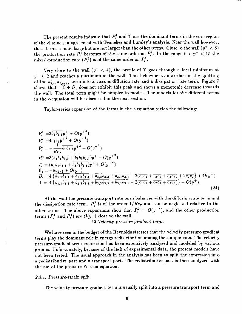
The present results indicate that P: and Y are the dominant terms in the core region of the channel, in agreement, with Tennekes and Lumley's analysis. Near the wall however, these terms remain large but are not larger than the other terms. Close to the wall (y+ < 8) the production rate P,' becomes of the same order as P,". In the range 6 < y+ < 15 the mixed-product.ion rate (P,") is of the same order as Pf'.

Very close to the wall (y+ < 4), the profile of Y goes through a local niininiuni at yS 2 2 and reaches a maximum at the wall. This behavior is an artifact of the splitting of the u ~ , , u ' , , , ~ ~ term into a viscous diffusion rate and a dissipation rate term. Figure 7 shows that - Y + D, does not exhibit this peak and shows a monotonic decrease towards the wall. The total term might be simpler to model. The models for the different terms in the c-equation will be discussed in the next section.

Taylor-series expansion of the terms in the c-equation yields the following:

At t,he wall the pressure transport rate term balances with the diffusion rate t,erin and the dissipat,ioIi rate term. P," is of the order 1/Re, and can be neglected relative to the other t,erms. The above expansions show that Pz = O(y+ ), and t,he other production terms (P,' and P,") are O(y+) close to the wall.

2.3 Velocity pressure-gradient terms

2

We have seen in the budget of the Reynolds stresses that the velocit,y pressure-gradient terms play the dominant role in energy redistribution among the components. The velocity pressure-gradient term expression has been extensively analyzed and modeled by various groups. IJnfortunat,ely, because of the lack of experimental data, the present models have not been test,ed. The usual approach in the analysis has been to split the expression into a redidributive part and a transport part. The redistributive part is then analyzed with the aid of the pressure Poisson equation.

2.3.1. Pressure-strain split

The velocity pressure-gradient term is usually split into a pressure transport term and

9

where &j = 2% (and S i j = (ul ,? . + u’. 311 . ) /2) is known as the pressure-strain term. Sub- stit.ut,ing the Taylor series expansion for pressure and velocities in the definition of 4ij

vields

For the case of a fully turbulent channel flow, the flow is homogeneous in the streamwise and spanwise directions and the split is irrelevant in these directions; II11 and I I 3 3 are the pressure-strain terms. The Taylor series expansions (eq. 26) show that the diagonal terms of +ij t-r 0 as y+ H 0, while the 4 1 2 component does not vanish at the wall.

Figure 8 shows the distribution across the channel of the terms obtained by splitting 1122 into a transport term and a pressure-strain term. In this case the split produces t,ernis that highly emphasize t,he presence of the wall. The reversal of the sign of the pressure-strain term near the wall was attributed by Moin & Kim (1982) to the “splatting” effect. The split chosen in equation (25) is not unique (Lumley, 1975); Launder (private communication, 1985) pointed out that the use of a decomposition suggested by Lumley:

where

would reduce the negat,ive levels of 4G2 near the wall to about one third their current, levels. A split suggested by the balance equation for the anisotropy tensor of the Reynolds stresses is as follows:

Note that the trace of &j is zero and therefore $ , j is redistributive. Figures 9-12 show the didribution across the channel of the terms in Eqs. (29) and (30). The negative levels of the redistributive 22 component near the wall are substantially reduced. In addition, the split suggests that a model for the trace of the velocity pressure-gradient term is needed rather than a model for the pressure-transport vector. This might be easier to achieve.

2.3.2. Fast and return splitting

10

An equation for the pressure fluctuation can be derived from the Navier-Stokes equa-

I t is customary (see Luinley 1978, for example) to split the pressure into two parts, p’ = pl + p 2 , one associated with the first term on the right-hand side of equation (31) and the other with the second and third terms. Most of the analyses used to model the pressure- st rain terms consider homogeneous cases where the boundary conditions are not considered in the split. The Poisson equation and the boundary conditions are linear in p . Therefore, we can isolate the effects of the viscous terms at the wall by splitting the pressure into three parts, a “return” part, a “rapid” part, and (for the case of flows with walls) a “Stokes” part. 3

i ) The rapid pressure, p l , is defined as the solution to the following problem:

(33 - a) P I . . 133 = -2Ui,juj,$ I

with the boundary conditions at the walls

Pty = 0

i i ) The return pressure, p 2 , is defined as the solution to

with the boundary conditions at. t,he walls

PTy = 0

iii) And finally t,he Stokes pressure, p s , is defined as the solution to

p . 7 0 S 913

(33 - b )

(34 - u )

(34 - b )

(35 - u )

with the boundary conditions at the walls

(35 - b ) S I p , , = v9YY

This split resolves the question of whether to add the boundary conditions to the return part of the pressure or to the rapid part. It does not remove the effect of the wall on the rapid and return pressure. The pressure-strain terms are linear in p and therefore

11

the St.okes pressure-strain statistics can be added to either the rapid pressure-strain terms or to the redurn pressure-strain terms.

The rapid part of the pressure-strain can be written analytically as follows:

where G is t,he Green function with homogeneous Neumann boundary conditions at the walls. Note that most modelers neglect the surface integral terms that should be added to equation (36) if inhomogeneous Neumann conditions are used for the pressure. The use of homogeneous boundary conditions (eq. 33 - b) at the walls for the rapid pressure is consist.ent with equat,ion (36) and the approximation used by the modelers. The effect of the wall on the pressure is contained in the form of the Green function G'.

Figures 13-16 show the splitting of the pressure-strain term into the three components. For the case of qhll the rapid part of the pressure-strain term is of the same order as the return part at y+ > 80. Close to the wall the return part is larger than the rapid part. The 4 2 2 terms show that at y+ > 80 most of the correlation is due to the return part. Near the wall, the rapid part in this case has the opposite sign from the total term. The total term is consuming close to the wall, while the rapid part is producing. The 433 terms show that the rapid part contributes the most to this component. Close to the wall the return part becomes the main contributor. The 9 1 2 split shows that at y+ > 80 the return and the rapid terms are of the same order. Close to the wall the return is the main contributor to the total term. The behavior of $12 near the wall is much more complicated than that of &I (eq. 30), which also suggests that it, might be simpler to model. Except for 9il, which is negligible throughout the channel, qhfJ for other components is significant only near the walls.

3. Model testing

In the previous sections we presented the budget data for the channel. In this section, we will use t,his data to evaluate some existing turbulence models. Our testing will be by direct comparisons of the ternis in the budget with the model expression using the chaiinel data.

3.1. Dissipation rate models

3.1.1. Algebraic models for cij

Rotta (1951a) argued that in the limit as Re H 0, the dissipation rate tensor will be aligned with the Reynolds stress tensor and can be modeled as

He also argued that in the limit Re H 00, the dissipation rate tensor is isotropic. This idea was used by HL2 who argued that the model for the dissipation rate tensor should

12

take the following form:

where t,hey inferred from the experimental data that fa is a function of the turbulence Reynolds number (IC’/€) as follows:

1 k2 10 €

fa = (1 + --)-’ (39)

The assumed form in equation (38) implies that the anisotropy tensor of the Reynolds st,ress and the anisot,ropy tensor for the dissipation rate are related as follows:

where dij = ~ j / ( 2 ~ ) - 6;j/3 and bij = =/(2k) 2 3 - bij/3.

Lumley and Newman (1977) identify a turbulence state in terms of the second (I1 ) and third (111 ) invariants of the Reynolds stress anisotropy tensor (b2,) . They have shown that turbulence states can be identified on a -11 vs. 111 map (anisotropy map) and that due to the properties of b,, , turbulence states are limited inside the region bounded by the two axisymmetric states and the two-dimensional state (see fig. 17). It can be shown that the states of the dissipation anisotropy tensor (dzj) are also contained in the same region as the b,, tensor (for more detail, see Lee & Reynolds, 1985). If we neglect the d13 and the d23 components of the tensor compared to the other components (for a large enough sample they are negligible), we can use the budget results presented in the previous section to compute the variation (as a function of g + ) of d,, on the anisotropy map. Figure 17 shows the points for d,, and b,, on the anisotropy map for different ys locations in the channel. Figure 18 shows the points for d,, and the curve for the right-hand side of equation (40). We note that the state of turbulence producing the dissipation rate tensor vary from a nearly isotropic state in the center of the channel to a two-dimensional state close to the wall. The model (eq. 40) clips the transition from the almost two-dimensional state near the wall to the state in the core region. Close to the center, the model is closer to the axisymmetric state than the data would indicate. The fact that the dissipation rate tensor is close to a two-dimensional state near the wall is an indication that the variation in d,, near the wall is due in part to wall-proximity. Near the wall, the normal component to the wall is suppressed and the anisotropy tensor approaches the line of the two-dimensional state. At around ys = 3.46 the state of the dissipation anisotropy tensor is closest to the one-dimensional state. The bij tensor will also vary from a two-dimensional state near the wall to the nearly isotropic state in the core region. In fact, if we assume that fa = 1 (; .e, that the anisotropy tensor of the dissipation rate and the anisotropy tensor of the Reynolds stress are equal), we find (fig. 17) better agreement between the data and the model. It is possible that this agreement is because KMM’s flow is at low Reynolds number. Comparison of the anisotropy invariant map of b,, with the map of d,, shows that

13

in the core region, the dissipation anisotropy is closer to the axisymmetric state than is the Reynolds stress anisotropy. We point out that close to the wall, Taylor-series expansions of d,, and b,, show that they are equal only up to O(ys). For example, d12 and b 1 ~ approach 0 as ys ++ 0, but the ratio of the two terms will yield dI2/b12 H 2 as y H 0. In fact, Launder & Reynolds (1983) proposed a model that will have the proper limits (for the ratio of the component of b,, and d, , ) , but using the values of the constants (a and P ) recommended by them will yield a model that is tensorially incorrect: e.g., the trace of and the trace of their model are not equal.

Figures 19-22 show t,he four components of ~ i j compared to the components of the model, t i j = E u : u > / k . The off-diagonal component shows the largest difference between the model and the data. The diagonal components show better agreements but would require a different function, fa, for the different components to obtain an improvement in the agreement.

3.1 2. Transport models for E .

-

Almost any type of one point closure models would require a time-scale or a length- scale model. Often, the dissipation rate of the turbulence kinetic energy is used to obtain these scales. In addition to the equations for the transport of the Reynolds stresses, an equation for the transport of the trace of E%, which is twice the dissipation rate of the turbulence kinetic energy, c (see eq. 23) is used. The terms in the equation of have been modeled by a number of workers (see for example Davydov, 1961; DH; HLl; Lumley & Khajeh-Nouri, 1974; HL2). Most of the current models for the €-equation can be written as the sum of a production term, a dissipation term, a turbulent transport, and a viscous

where Pk = Pll/2 is t,he production rate of the turbulence kinetic energy, Ccl, C62, and C,', are const,ants or functions of the turbulence Reynolds number. The disagreement' is in t,he correspondence of the modeled expression with the exact equation. Lumley and Khajeh-Nouri (1974); and later HL2, associated the right-hand side of equation (41) with the difference between Pp and Y (see eq. 23) and did not identify a model for each term in the balance equation. Davydov (1961) and HL1 combined the production terms P: and P: and modeled them as follows:

€- € P,' + P, 2 = -c,1 -u;u;sij = ccl- Pk k k

HL2 recommend C,l = 1.275. Figure 23 shows the above model compared to the data; t,he agreement is good away from the wall. The model predicts the production very well away from the wall. In the near wall region, however, the peak in the production of c is underpredicted and a modification to the model is needed in this region.

HL1 combined the production term P: with Y and modeled the combination as

€2

k -Pp + Y = Cr2- (43)

14

The right-hand side of equation (43) approaches 00 as y I-+ 0. HL2 modified the model for t,he dissipation rate of c using a modified dissipation rate of k, Z = c - 2 ( ( l ~ ' / ~ ) , ~ + ) )

which insures that the ratio Z / k is bounded as y+ H 0. They also argued that turbulence data indicate t,hat the dissipation rate of c is a function of the Reynolds number. This functional was accounted for by introducing a damping function. If t.he model of HL2 represents a model for the left-hand side of equation (43), we have

2

c; -p:sr=c "'k f - (44)

where Cc2 = 1.8, and fc = 1. .- & exp [ - ( k 2 / 6 c ) 2 ] . Figure 24 shows the above model compared to the data. In the core region, the model and the data show good agreement. Close to the wall, the model underpredicts the data.

The turbulent transport of c is modeled by HL1 as

where Cyc = 0.15. Figure 25 shows the model compared to the data. This term is small compared t.0 the other terms in the budget equation and the disagreement between the model and t,he data is small compared to the errors in the other terms. The production rat,e, P$, and t,he pressure diffusion rate, ne, were neglected by HL1, and the present, data also show t,hat, these terms are small.

3.2. Pressure-strain models

Most models used for the velocity pressure-gradient expression are based on splitting the expression into a pressure-strain term and a pressure diffusion term. The pressure diffusion term is either added to the turbulent transport term or neglected. Several models for the pressure-strain term exist that use different approximations and arguments to provide closures for the term. Most of these closures are based on homogeneous flow arguments. In this section, we will test the closure of LRR for the pressure-strain term that was developed for wall-bounded flows. LRR split the pressure-strain term into a return term, a rapid term, and a wall term. For the return terms, 4:1) they recommend the use of the model proposed by Rotta (1951a),

where c11 is a model constant,. They modeled the rapid term by assuming that. t.he mean velocity gradient is slowly varying and write

41. 2 3 = u,,,a;i (47)

They then assumed that a;' is linear in the Reynolds stresses. Substitution of the linear approximation for ugi into the expression for (p:j yields

15

- I where, A;j = -(u',uiUk,j + U > U i U k , i ) . The above model also has one adjustable constant,

CY2. The value of the constants C1 = 1.5 (for the return term) and G2 = 0.4 were chosen by LRR by matching the homogeneous shear experiment of Champagne, Harris, & Corrsin (1970).

By examining the case of wall bounded flows, LRR argued that a third term, d:;, is needed to account, for near-wall effects, corresponding to the reflected wall influence of 4tJ + @ j . They argued that t,he model for the wall effects should take the same form as 4:1 + 4;) and using near-wall data, the wall effect on the pressure-strain was modeled as

Figures 26-28 show comparisons of LRR's model for the diagonal terms to the data. The comparison for the off-diagonal term is similar, the agreement is acceptable away from the wall, but is poor close to the wall. We have also shown the distribution of the individual terms. Rotta's return model does not vanish at the wall; while, as can be seen from the Taylor series expansions (eq. 26), the diagonal terms should vanish at the wall. This is an indication that LRR's model will behave poorly close to the wall because of the return model. It is clear that Rotta's model should be modified to include the correct behavior near the wall. In fact, the model without Rotta's return model shows the proper trends, and it will be better than the full model.

3.3. Turbulence transport models

The nonlinearity of the equations of motion introduces higher order moments when equations for the moments are derived. For the Reynolds-stress equations, the triple- correlation terms need either t.o be closed or to have an equation derived for them. The need for equat,ions describing the evolution of the turbulent transport term (Tijk = u'.ul.uL) was suggest,ed by Chou (1945a) and Davydov (1959). But using closures at the triple- correlat,ion level will add ten more equations to the system of equat.ions to be solved. How- ever, the transport equations for Tijk are used to derive closures for the triple-correlation t.erms. The construct.ion of t,he model for the t,ransport terms start.s (see HL1; and Lumley, 1978) with the governing equation for the transport terms,

z ?

I l l 1 1 1 1 1 1 1 1 1 +(uIui"juL),l = -(ujukp,i + uiujp,k + U L U i p l j ) + {u!juiuI,,, + uiujuk,l[ + uiu:u>,,,)

(50) Davydov neglected the second term on the right-hand side of equation (50). He also argued t,hat in an analogy to the pressure-strain model, the remaining term on the right.- hand side should be modeled as -Cbc/k Tijk. To close the quadruple-correlation term, Millionshchikov's zero-fourth-cumulant hypothesis (Monin & Yaglom 1975, p. 241 ) is often

16

Using the above closure in the triple-correlation equations, we have

If we use the assumption of HL1 (that the transport terms are in equilibrium) and - drop the & term, the model for the triple correlation will close as follows:

In addition to the equilibrium assumption, HL1 assumed that the production terms are negligible and wrote the model for the triple correlation as follows

__- -__ k -- -IL;u;u> = C d - { I L : I L { ( I L > I L L ) , / , € + IL>IL',(IL;u:),1 + IL;ui(ILiu>),[} (54)

For the case of no mean velocity gradients, the two models (eqs. (53) and (54)) are the same (with Cb = l/Cs). If we use the expression given by equation (53) to model the transport terms, we have for the channel case

-- -I- ULIL; (IL\IL\ ) ,Z + 2U1,2Tglg]

k- - -T222 = c,-u;IL; (UL?4),2

€

-- -T233 = Cs-

The above expressions show that the production of the triple correlation in the fully de- veloped channel will affect the 2'211 and T212 components only; the largest effect is on the Tgll component. Figure 29 shows the models for T211 given by equations (53) and (54) (with Cs = l/Cb = .11) compared to the data. These results indicate that both models do not agree well with the data and that including the production term does not improve the model. The extra effort involved in inverting the coupled system given by equation (53) is not justified.

A simpler form for the transport terms was derived by DH using the recipe that, turbulence transport of a quantity, I L L # , should be modeled as cx u;u; +,[. Following this recipe, they modeled the transport term as

- --

17

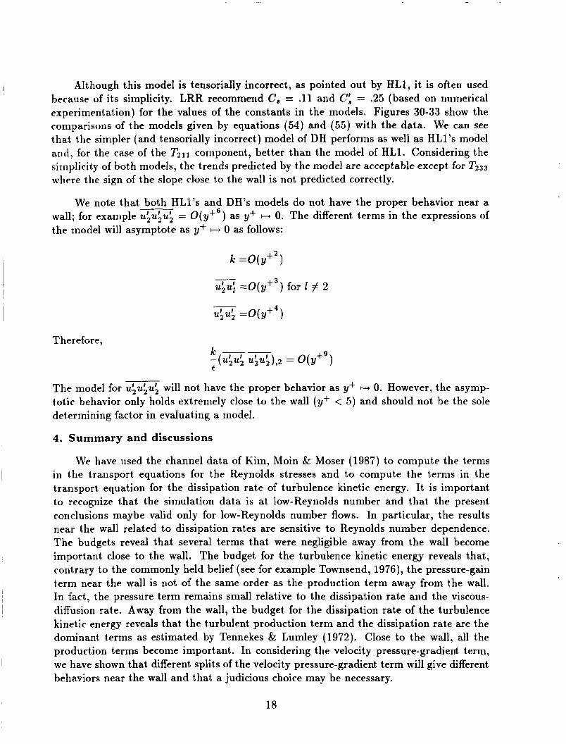
I Although this model is tensorially incorrect, as pointed out by HL1, it is often used because of its simplicity. LRR recommend C, = .ll and C: = .25 (based on numerical experimentation) for the values of the constants in the models. Figures 30-33 show the comparisons of the models given by equations (54) and ( 5 5 ) with the data. We can see that the simpler (and tensorially incorrect) model of DH performs as well as HLl's model and, for the case of the 2'211 component, better than the model of HL1. Considering the simplicity of both models, the trends predicted by the model are acceptable except for 7'233

where the sign of the slope close to the wall is not predicted correctly.

We note that both HLl's and DH's models do not have the proper behavior near a wall; for example uLuku.; = O ( Y + ~ ) as y+ H 0. The different terms in the expressions of the model will asymptote as y+ H 0 as follows:

k = O ( Y + ~ )

Therefore,

The model for T L ~ U ; U ; will not have the proper behavior as ys H 0. However, the asymp- totic behavior only holds extremely close to the wall (ys < 5 ) and should not be the sole degermining factor in evaluating a model.

4. Summary and discussions

We have used the channel data of Kim, Moin & Moser (1987) to compute the terms in the transport equations for the Reynolds stresses and to compute the terms in the transport equation for the dissipation rate of turbulence kinetic energy. It is important to recognize that the simulation data is at low-Reynolds number and that the present conclusions maybe valid only for low-Reynolds number flows. In particular, the results near the wall related to dissipation rates are sensitive to Reynolds number dependence. The budgets reveal that several terms that were negligible away from the wall become important close to the wall. The budget for the turbulence kinetic energy reveals that, contrary to the commonly held belief (see for example Townsend, 1976), the pressure-gain term near the wall is not of the same order as the production term away from the wall. In fact, the pressure term remains small relative to the dissipation rate and the viscous- diffusion rate. Away from the wall, the budget for the dissipation rate of the turbulence kinetic energy reveals that the turbulent production term and the dissipation rate are the dominant terms as estimated by Tennekes & Lumley (1972). Close to the wall, all the production terms become important. In considering the velocity pressure-gradient term, we have shown that different splits of the velocity pressure-gradient term will give different behaviors near the wall and that a judicious choice may be necessary.

18

For wall-bounded flows, we have shown that the inhomogeneous boundary condition on the pressure introduces a third term in the split of the pressure and have recommended that the pressure be split into a rapid term, a return term, and a Stokes term. We find that the rapid and the return terms in the channel are of the same order, and we cannot neglect one with respect to the other. The 22 component of the pressure-strain term shows that the rapid part in fact has the opposite sign as the total term. Away from the wall the rapid part is consuming, while the total term is producing. Close to the wall the tot a1 term is consuming (the splatting effect), while the rapid part is producing.

Comparison of closure models with the data reveals that the pressure-strain term needs immediate attention and the model of Launder, Reece & Rodi (1975) has difficulty. As a first approximation, the anisotropy tensor for the dissipation rate of the Reynolds stresses may be modeled in terms of the anisotropy tensor of the Reynolds stresses. The budget for the dissipation rate of the turbulence kinetic energy is modeled well away from the wall; close to the wall, improvements are needed. Finally, the transport term also can be improved upon. Overall, the closure models are better than expected for the budget of the dissipation rate of the turbulence kinetic energy and are generally inadequate for the pressure-strain correlations.

19

REFERENCES

Champagne, F. H., Harris, V. G. & Corrsin, S. 1970 Experiments on nearly homoge- neous shear flow. J. Fluid Mech. 41, 81.

Chapman, D. R. & Kuhn, G. D. 1986 The limiting behavior of turbulence near a wall. J. Fluid Mecli. 170, 265-292.

Chou, P. Y. 1945a On velocity correlations and the solutions of the equations of turbulent fluctuations. Q. Appl. Math. 3, 38-54.

Chou, P. Y. 1945b Pressure flow of a turbulent fluid between parallel plates. Q. Appl. Math. 3, No. 3, 198-209.

Daly, B. J. & Harlow, F. H. 1970 Transport equations in turbulence. Phys. Fluids 13, NO. 11, 2634-2649.

Davydov, B. I. 1959 On the statistical dynamics of an incompressible turbulent fluid. Dokl. Akad. Nauk SSSR 127, No. 5, 768-770 (Trans. in Soviet Physics-Doklady 4, No. 5, 1960, 769-772).

Davydov, B. I. 1961 On statistical dynamics of an incompressible turbulent, fluid. Dokl. Akad. Nauk SSSR 136, No. 1, 47-50 (Trans. in Soviet Physics-Doklady 6, No. 1, 1961, 10-12).

Hanjalit, E(. & Launder, B. E. 1972 A Reynolds stress model of turbulence and its application to thin shear flows. J. Fluid Mecli. 52, part 4, 609-638.

Hanjalit, Ii. & Launder, B. E. 1976 Contribution towards a Reynolds-stress closure for low-Reynolds-number turbulence. J. Fluid Mech. 74 part 4, 593-610.

Kim, J., Moin, P. & Moser, R. 1987 Turbulence statistics in fully developed channel flow at. low Reynolds number. J. Fluid Mech. 177, 133-166.

Kolmogorov, A. N. 1942 Equation of turbulent motion of an incompressible fluid. Izv. Akad. Nauk SSSR, Ser. Fiz. 6, 56-58.

Launder, B. E., Reece, G. J. & Rodi, W. 1975 Progress in the development of a Reynolds-stress turbulence closure. J. Fluid Mech. 68 part 3, 537-566.

Launder, B. E. & Reynolds, W. C. 1983 Asymptotic near-wall stress dissipation rates in a turbulent flow. Phys. Fluids 26, No. 5, 1157-1158.

Lee, M. J. & Reynolds, W. C. 1985 Numerical experiments on the structure of homo- geneous turbulence. Report No. TF-24. Department of Mechanical Engineering. Stanford {Jniversity, Stanford, CA.

Lumley, J. L. 1975 Pressure strain correlation. Phys. Fluids 18, 750.

Lumley, J. L. 1978 Computational modeling of turbulent flows. Advances in Applied

20

Mech. 18, 123-176.

Lumley, J. L. & Khajeh-Nouri, B. 1974 Computational modeling of turbulent trans- port,. Turbulent. Diffusion in Environmental Pollution, Ed. F. N. Frenkiel & R. E. Munn, Advances in Geoph. 18A, 169-192, Academic Press., NY.

Lumley, J. L. & Newman, G. R. 1977 The return to isotropy of homogeneous turbu- lence. J. Fluid Mech. 82, part 1, 161-178.

Moin, P. & Kim, J. 1982 Numerical investigation of turbulent channel flow. J. Fluid Mech. 118, 341-377.

Monin, A. S. & Yaglom, A. M. 1975 Statistical Fluid Mechanics: Mechanics of Turb- ulence. 2, Ed J. L. Lumley, MI'I' Press, Cambridge, Mass.

Moser, R. D. & Moin, P. 1984 Direct Numerical Simulation of Curved Turbulent, Channel Flow. NASA T M 85974. Ames Research Center, Moffett Field, CA.

Rogallo, R. S. 1981 Numerical experiments in homogeneous turbulence. NASA T M 81315, Ames Research Center, Moffett Field, Ca.

Rotta, J. 1951a Statistical theory of inhomogeneous turbulence, Part 1. Zeitschrift f u r Physik 129, 257-572.

Rotta, J. 1951b Stat8ist.ical theory of nonhomogeneous turbulence, Part 11. Zeif.sclirift fur Physik 131, 51-77.

Shih, T-H. & Lumley, J. L. 1986 Second-order modeling of near-wall turbulence. Phys. Fluids 29, No. 4, 971-975.

Spalart, P. R. 1986a Numerical study of sink-flow boundary layers. J. Fluid Mech. 172, 307-328.

Spalart, P. R. 1986b Direct Simulation of a Turbulent Boundary Layer up to Re = 1400, NASA T M 89407. Ames Research Center, Moffett Field, CA.

Tennekes, H. & Lumley, J. L., 1972 A First Course in Turbulence. MIT Press, Cam- bridge, Mass.

Townsend, A. A. 1976 The structure of turbulent shear flow. Cambridge University Press, Cambridge, England.

21

0.5

Gain 0.3

0.1

-0.1

LOSS -0.3

0.0 50.0 100.0 150.0

Y+

Terms in the budget of u\u\ in wall coordinates. Pll = Production; TI1 = Turbulent transport; Dl1 = Viscous diffusion; €11 = Dissipation rate; 1111 = Velocity pressure-gradient taerm.

- Figure 1.

Gain

Loss

0.03

0.02

0.01

0.00

-0.01

-0.02

0.0 50.0 100.0 150.0

Y+ ,

Figure 2. Terms in the budget of uiui in wall coordinates. 2'22 = Turbulent transport; 0 2 2 = Viscous diffusion; € 2 2 = Dissipation rate; lI22 = Velocity pressure- gradient term.

22

Gain

Loss

0.10

0.05

0.00

-0.05 - E33

0.0 50.0 100.0 150.0

Y+ -

Figure 3. Terms in the budget of u ~ u ~ in wall coordinates. 2'33 = Turbulent transport; 0 3 3 = Viscous diffusion; €33 = Dissipation rate; II33 = Velocity pressure- gradient term.

Gain

Loss

0.08

0.04

0.00

-0.04

I - . /

0.0 50.0 100.0 150.0

Y+ -

Figure 4. Terms in the budget of u:ui in wall coordinates. PI2 = Production; TI, = Turbulent transport; 0 1 2 = Viscous diffusion; €12 = Dissipation rate; III2 = Ve1ocit.y pressure-gradient, ratme.

23

Gain

Loss

0.2

0.1

0.0

-0.1

50.0 100.0 150.0 0.0

Y+ Figure 5 . Terms in the budget of the turbulence kinetic energy, I C , in wall co-

ordinat,es. Pk = Production; Tk = Turbulent transport; Dk = Viscous diffusion; e k = Dissipation rate; n k = Velocity pressure-gradient term.

0.03

0.02

0.01

0.00

-0.01

-0.02

Gain

Loss

0.0 20.0 40.0 60.0

Y+ Figure 6. Terms in the budget of the dissipation rate of t2he turbulence kinetic

energy, e , in wall coordinates. P,] = Production by mean velocity gradient; P: = Mixed production; P: = Gradient production; P: = Turbulent production; T, = Turbulent pransport; D, = Viscous diffusion; T = Dissipation rate; 11, = Pressure transport.

24

0.03

0.02

-0.01

-0.02 - - - - Y - - - - - I I I 1 1 I l I I I I l l I I 1 1 1 1 I 1 1 I 1 1

0.0 20.0 40.0 60.0

Y+ Figure 7.

diffusion term, D,. Split of the viscous term into a dissipation rate term, Y, and a viscous

4 P I 2

(m) .2

0.03

0.02

0.01

0.00

-0.01

-0.02

0.0 50.0 100.0 150.0

Y+ Figure 8. Split of the velocity pressure-gradient term into a pressure transport -

term, and a pressure-strain term, pu: +. IY

25

0.02

0.00

n11

u3ui -0.02 -l-h 2k

rill -0.04 n 1 1 - - U l U l

2k

-0.06

0.0 50.0 100.0 150.0

Y+

Figure 9. Split of the velocity pressure-gradient term, n11, into a pressure transport t,erni, u i u i / 2 k nil, and a redistributive term, - u i u i / 2 k nil.

0.03

0.02 n22

0.00

50.0 100.0 150.0 0.0

Y+ Figure 10. Split, of the velocity pressure-gradient term, n22, into a pressure

t.ransport, term, u',u',/2k rill, and a redistributive term, IIZ2 - uLu;/2k I I l l . -

26

0.08

ugu2 2k n11 0.04

215 u3 rill n33 - - 2k 0.02

0.00

0.0 50.0 100.0 150.0

Y+

Figure 11. Split of the velocity pressure-gradient term, Il33, into a pressure transport term, uLu5/2k IIll, and a redistributive term, II33 - u~u:/2k IIll.

0.08

0.06 n 1 2

ui ui 0.04 --rh

rill 0.02 21: u2

2k

n12 -

0.00

0.0 50.0 100.0 150.0

Y+ Figure 12. - Split of the velocity pressure-gradient term, Ill,, into a pressure

transport term, u\uh/2k IIll, and a redistributive term, I l l 2 - u\uk/2k I l l l .

27

0.06

0.04

0.02

0.00

-0.02

-0.04

-0.04

0.0 50.0 100.0 150.0

Y+

- - -

- - - - - - ; l l l l l l l l l l ' l l l l l l l l ' l l l l l l l l l ' l l l l l '

Figure 13. and a St,okes term, 4f1.

Split of pressure-strain term, $11, int,o a rapid t,erm, 4il, a return t,ernl,

4222 7

28

0.06

0.04

0.02

0.00

-0.02

-0.04

0.0 50.0 100.0

Y+

150.0

Figure 15. and a Stokes term, &.

Split of pressure-strain term, $33, into a rapid term, 4i3, a return t,erm,

0.08

0.06

0.04

0.02

0.00

-0.02

0.0 50.0 100.0

Y+

150.0

Figure 16. and a Stokes term, c$:~.

Split of pressure-strain term, $12, into a rapid term, 4i2, a ret,urn term,

29

-11

0.3

0.2

0.1

/ y+ = 3.46

L /,

0.00 0.01 0.02 0.03 0.04 0.05 0.06 0.07 0.08 111

Figure 17. Anisotropy invariant map. o o o o dij at various y+ in the channel; bij at various y+ in the channel.

-11

0.3

0.2

0.1

0.00 0.01 0.02 0.03 0.04 0.05 0.06 0.07 0.08

111

Figure 18. Anisotropy invariant map. o o o o di j at various ys in the channel; model, equation (40).

30

€11

0.30

0.25

0.20

0.15

0.10

0.05

0.0 50.0 100.0 150.0

Y+ Figure 19. Distribution of €11 across the channel. o o o o €11 term computed from

the channel data; - model, c / k uiu;.

0.05

0.04

0.03 E22

0.02

0.01

0.0 50.0 100.0 150.0

Y+ Figure 20. Distribution of €22 across the channel. o o o o €22 term computed from

the channel data; - model, uhui.

31

0.10

0.08

0.01

0.00

-0.01

-0.02

-0.03

E. 12

-0.04

0.06 € 3 3

0.04

0.02

50.0 100.0 150.0 0.0 Y+

Figure 21. Distribution of €33 across the channel. o o o o €33 term computed from the channel data; - model, c / k uiui.

0.0 50.0 100.0 150.0

Y+

Figure 22. Distribution of €12 across the channel. o o o o €12 term computed from the channel data; - model, c / k uiu;.

32

0.03

. r - - - - - - - - -

1 1 1 1 1 1 1 1 1 1 1 1 1 1 1 1 1 1 1 1 1 1 1 1 1 1 1 1 1 1 1 1 1 1 1 1 1 1 1 1 1 1 1 1 1 1 1 1 1 1 1 1 1 1 1 1 1 1 1

0.02

P,' + P,2 0.01

0 1 oooo

0 c n

0.00

0.0 10.0 20.0 30.0 40.0 50.0 60.0

YS Figure 23. Distribution of the production term, P,] + P:, in the budget of c across

t,he channel; o o o o term computed from the channel dat,a; - model, equation (42) .

Pp - Y

0.01

0.00

-0.01

-0.02

p o 0

0 0

0.0 10.0 20.0 30.0 40.0 50.0 60.0

w+ Figure 24. Distribution of the dissipation term, P: - Y, in the budget of across

t,he channel. o o o o term computed from the channel data; - model, equation (44).

33

0.01 E

!-

-0.01 k -0.02

0.0 10.0 20.0 30.0 40.0 50.0 60.0

Y+ Figure 25. Distribution of the turbulent transport term, T,, in the budget of 6

across t,he channel. o o o o term computed from the channel data; - model, equa-

t.ion (45).

P4.1

0.0

-0.2

0.0 50.0 100.0 150.0

Y+

I Figure 26. Pressure-strain term, p ~ i , ~ , in the budget equation for U ~ U ; across t ne

model, channel. o o o o term computed from the channel data;

(eq. (48)+eq. (49)). model, (eq. (46)+eq. (48)+eq. (49)); ---- model, equation (46);

34

P 4 . 2

0.20

0.15

0.10

0.05

0.00

0.0 50.0 100.0 150.0

Y+ Figure 27. Pressure strain term, pui,,, in the budget equation for ukuk across t,he

model, (eq. (46)+eq. (48)+eq. (49)); ---- model, equation (46). - - model, channel. o o o o term computed from the channel data;

(eq. (48)+eq. (49)). 0.20

0.15

0.10 P 4 , 3

0.05

0.00

0.0 50.0 100.0 150.0

Y+ Figure 28. Pressure strain term, P U ; , ~ , in the budget equat,ion for uiu i across the

model, channel. o o o o term comput,ed from the channel data;

(eq. (48)+eq. (49)). model, (eq. (46)+eq. (48)+eq. (49)); ---- model, equation (46).

35

~

- u p l u'l

1.5

1.0

0.5

0.0

-0.5

-1.0

E-

0.0 50.0 100.0 150.0

YS

Figure 29. Triple correlation term -u;uiui across the channel. o o o o term computed from the channel data; - model, equation (53); - - - - model, equation (54).

-u;u'lu'l

1 .o

0.5

0.0

-0.5 t

-1.0

0.0 50.0 100.0 150.0

Y+ Figure 30. Triple correlation term -uIuiu\ across the channel.

o o o o term computed from the channel data; - model, equation (54); ---- model, equation (55).

36

-u;u;u;

0.250

0.125 0

0

0.000

-0.125

0 0

0

0 0

0

0.0 50.0 100.0 150.0

YS Figure 31. Triple correlation term - u L u ~ u ~ across the channel.

o o o o term computed from the channel data; - model, equation (54); - - - - model, equation (55).

0.15 E- t

0.10

0.05

0.00

-0.05

-0.10 c

0.0 50.0 100.0 150.0

YS Figure 32. Triple correlation term - u ~ u . ~ u ~ across the channel.

o o o o term computed from the channel data; - model, equation (54); - - - - model, equation (55) .

37

0.2 Oe4 i 0

0

0

o o o o o 0 O O

0 0

0 0

0 0

0 0

0 0 0 0

Figure 33. Triple correlation t,erxii -u~u\u~ across the channel. o o o o term computed from the channel data; - model, equation (54); - - - - model, equation (55) .

38

Report Documentation Page

2. Govciiiiiieiit Accession No. 1 I. n c p w NO. NASA TM-8945 1

-------I- 4. Title end Sul)title

Rcynolds-Stress and Dissipation Rate Budgets in a Turbulent Channel Flow

7. Aulliorlsl

N. N. Mansour, J . Kim, and P. Moin*

9. Performing Organization Name end Address

Ames Research Center Moffett Field, CA 94035 I- ----- - 2. Sponsoring Agency Name end Address

National Aeronautics and Space Administration Washington, DC 20546-0001

December 1987 . - ... .... ~- ..

6. Perfotniiiig Orgniiizntioii Cocln

A-87 182

505-60 - - -- - -- .- 11. Contract or Grant No.

Technical Memorandum __ .. - _ _

14. Sponsoring Agency Cock

... -- ........

5. Sul)plementary Notes

*Also Dept. of Mechanical Engineering, Stanford University, Stanford, CA 94035 Accepted for publication in J . Fluid Mech. Point of Contact: N. N. Mansour, Ames Research Center, MS 202A-1, Moffett Field, CA 94035

(41 5) 694-6420 or FTS 464-6420

.The budgets for the Reynolds stresses and for the dissipation rate of the turbulence kinetic energy are computed using direct simulation data of a turbulent channel flow. The budget data reveal that all the terms in the budget become important close t o the wall. For inhomogeneous pressure boundary conditions, the pressure-strain term is split into a return term, a rapid term, and a Stokes term. The Stokes term is important close t o the wall. The rapid and return terms play different roles depending on the component of the term. A split of the velocity pressure-gradient term into a redistributive term and a diffusion term is proposed, which should be simpler to model. The budget data is used to test existing closure models for the pressure-strain term, the dissipation rate, and the transport rate. In general, further work is needed to improve the models,

. -_ - ....... 1. Key Words lSuggosted by Autlior(s)l ‘TIE. Distribuiionstaternent

Reynolds stress budget Dissipation rate budget Turbulence modeling Turbulent channel flow

Unclassified-Unlimi ted

Subject Category - 34 --_----I--- 20. Swurity Classif. (of this page) i-?kurity Clessif. lo1 this report1

Unclassified -----I Unclassified

NASA FORM 1626 OCT 86 For sale by the National Technical Information Service, Springfield, Virginia 2216 1

._ 22. Price

AQ 3