Turbulent Statistics from Time-Resolved PIV · PDF fileTurbulent Statistics from Time-Resolved PIV Measurements of a Jet Using Empirical Mode Decomposition ... -0.45-0.40-0.35 0.64

Turbulent Statistics from Time-Resolved PIV

Measurements of a Jet Using Empirical Mode

Decomposition

Milo D. Dahl∗

NASA Glenn Research Center, Cleveland, OH, 44135, USA

Empirical mode decomposition is an adaptive signal processing method that when ap-plied to a broadband signal, such as that generated by turbulence, acts as a set of band-passfilters. This process was applied to data from time-resolved, particle image velocimetrymeasurements of subsonic jets prior to computing the second-order, two-point, space-timecorrelations from which turbulent phase velocities and length and time scales could bedetermined. The application of this method to large sets of simultaneous time histories isnew. In this initial study, the results are relevant to acoustic analogy source models forjet noise prediction. The high frequency portion of the results could provide the turbulentvalues for subgrid scale models for noise that is missed in large-eddy simulations. The re-sults are also used to infer that the cross-correlations between different components of thedecomposed signals at two points in space, neglected in this initial study, are important.

I. Introduction

Computational approaches to predicting jet noise may be categorized as acoustic analogy and numericalmethods. The acoustic analogy methods use a rearrangement of the governing equations. The resultingequation contains a linear operator on one side of the equation that reduces to the wave equation foracoustic propagation at large distances from the source region. On the other side of the equation are termsthat are significant within a relatively small region and are identified as the equivalent or analogous acousticsources. The formal solution for the acoustic spectrum in the far field typically involves a convolution integralcontaining a wave propagator function and a correlation function of turbulence terms in the flow field.1

Numerical methods based on direct numerical simulation attempt to compute all the scales of turbulence ina flow followed by the computation of the associated radiated noise field. This type of computation requiresa large amount of computer resources and time. Using less computer resources, large-eddy simulationscompute the relatively larger scales of turbulence in the jet flow field. Consequently, higher frequency noiseis missing from the resulting acoustic field spectrum calculations since the computational grid is too largeto capture the turbulent noise sources at smaller subgrid scales. Thus, subgrid scale noise models have beenproposed following the acoustic analogy approach.2 Whether the full acoustic spectrum or just the highfrequency portion of the acoustic spectrum is to be predicted, these methods require turbulence statisticsfrom flow field measurements. Bodony & Lele,3 using spatial filtering of a highly resolved, direct numericalsimulation of a two-dimensional, low-Reynolds-number shear layer, computed the statistics for both theresolved, large-eddy-simulation-type scales and the unresolved, subgrid scales of turbulence. The parametersfor the spatial filter had to be determined prior to its use. In this paper, empirical mode decomposition isused on measured data from jets to filter the data and separate the turbulent scales prior to the computationof turbulent statistics. The decomposition effectively filters the data in a manner that is automatic andsignal dependent.

Empirical mode decomposition (EMD) is a recently developed, adaptive signal processing method for anygeneral, non-stationary, and nonlinear signal.4 The method separates the data signal into a series of basisfunctions, called intrinsic mode functions, using the data itself. The intrinsic mode functions (IMFs) derivedfrom signal decomposition have been used to distinguish physical phenomena of different frequencies and

∗Senior Research Scientist, Senior Member AIAA

1 of 20

American Institute of Aeronautics and Astronautics

https://ntrs.nasa.gov/search.jsp?R=20120018039 2018-05-23T21:38:03+00:00Z

wavelengths regardless of the long or short duration of the signal. For example, the method has been appliedto study classical nonlinear systems, wind and water wave interactions, ocean waves and tides, tsunamiwaves, seismic waves, and atmospheric turbulence.5 The newness of the method and its current issues, suchas its limited mathematical foundation and uniqueness,6 have not slowed its successful application. Aftera description of the velocity field measurements using time-resolved, particle image velocimetry (TR-PIV)and the jet operating conditions, a description is given of the EMD method as applied in this study. Theapplication of EMD on a large set of simultaneous time histories generated by TR-PIV and subsequentlycomputing two-point, space-time correlations is new.

This paper provides some initial results determined from the second-order, two-point, space-time correla-tions and spectra computed using the total signals consisting of the flow velocity time histories from TR-PIVand the IMFs of the decomposed signals. Surveys of the axial fluctuating velocity signal and the IMF com-ponents of the decomposed signal space-time correlations are given at three reference points near the liplineof two subsonic jets. From the correlations, turbulence phase velocities and integral length and time scalesare determined. For the higher speed jet of the two measured jets, the frequency dependent version of theseturbulence values are presented and compared to the correlation derived values. It is the highest frequencyIMF results for the phase velocities and the length and time scales that may be applicable to subgrid scalenoise source modeling. Finally, as a prelude to future work, the importance of the cross-correlation betweenIMFs is considered.

II. Description of Test Measurements

An extensive set of measured jet noise and flow data has been acquired using the Small Hot Jet AcousticRig at the NASA Glenn Research Center.7 Included in that set is data from time-resolved, particle imagevelocimetry (TR-PIV). Using this technique, velocity fields were measured in a jet flow at resolutions inboth space and time suitable for computing spatial-temporal correlations and spectra. The details of thetechnique and the methods of data acquisition are found in Wernet8 and in Bridges & Wernet.9 Data fromjets issuing from a converging nozzle with exit diameter D = 50.8 mm operating at exit Mach numbers of0.51 and 0.98 were used in this paper. The operating conditions for both jets, respectively labelled SP3 andSP7, are shown in Table 1 where Tt/T∞ is the total temperature ratio relative to ambient conditions, Ts/T∞is the static temperature ratio, Pt/P∞ is the nozzle pressure ratio, MJ is the jet Mach number, UJ/c∞ isthe jet acoustic Mach number, UJ is the jet exit velocity, and c∞ is the ambient speed of sound.

Case Tt/T∞ Ts/T∞ Pt/P∞ MJ UJ/c∞ UJ(m/s)

SP3 1.00 0.95 1.20 0.51 0.50 172.8

SP7 1.00 0.84 1.85 0.98 0.90 310.0

Table 1. Test conditions for convergent nozzle flow measurements.

As discussed in Wernet,8 the size of the TR-PIV measurement field depends on the sampling or cameraframing rate. The higher the sampling rate, the smaller the field of view becomes. With additional consid-erations such as the amount of storage space available for the data, the amount of data that can be obtaineddetermines the length of the time histories for the TR-PIV measurements. The jet cases listed in the tablewere sampled at 25 kHz with a time history length of about 1 second resulting in the maximum Strouhalnumber for analysis of 3.67 for case SP3 and 2.05 for case SP7 with resolutions in Strouhal number of 0.014and 0.008, respectively. The measured field was 178.85 mm wide in the axial direction and 5.18 mm widein the radial direction with a discretization of 70 by 5. The spatial resolutions are ∆x/D = 0.0510 and∆r/D = 0.0255. Figure 1 shows a representation of the nozzle and the three TR-PIV measurement locationswith equal scale in the r/D and x/D direction.

Mean and turbulence quantities computed from the measured TR-PIV data are shown in Figures 2to 4. The mean axial velocity contours in Figure 2 reflect the wide disparity between the axial and radialdimensions. The negative sign on the radius is maintained by convention with the measurement coordinates,indicating that the measurements were made near the lipline below the centerline of a horizontal jet as shownin Figure 1. Line plots along each of the five radial measurement locations are shown for the normalizedmean axial velocity in Figure 3. The lowest mean axial velocities occur along the line r/D = −0.49, nearestto the lipline of the jets. Figure 4 shows a similar set of line plots for the normalized axial turbulence

2 of 20


x/D

r/D

-4 -2 0 2 4 6 8 10 12 14

-2

0

2

Figure 1. TR-PIV measurement domain size and location relative to the nozzle.

x/D

r/D

2 4 6 8 10 12 14-0.50

-0.45

-0.40

-0.350.64 0.7 0.76 0.82 0.88 0.94

(a) SP3 jet with MJ = 0.51, Tt/T∞ = 1.00

x/D

r/D

2 4 6 8 10 12 14-0.50

-0.45

-0.40

-0.350.64 0.7 0.76 0.82 0.88 0.94

(b) SP7 jet with MJ = 0.98, Tt/T∞ = 1.00

Figure 2. Mean axial velocity contour plots.

x/D

Mean(u)/U

J

2 4 6 8 10 12 14

0.6

0.8

1.0


x/D

Mean(u)/U

J

2 4 6 8 10 12 14

0.6

0.8

1.0


Figure 3. Mean axial velocities at 5 equidistant radial locations from about r/D = −0.39 to −0.49. Arrow points towardvelocities at increasing radius. Dot marks reference point conditions.

x/D

Mean(u’u’)/U

J2

2 4 6 8 10 12 14

0

0.01

0.02

0.03


x/D

Mean(u’u’)/U

J2

2 4 6 8 10 12 14

0

0.01

0.02

0.03


Figure 4. Axial turbulence intensities at 5 equidistant radial locations from about r/D = −0.39 to −0.49. Arrow pointstoward turbulence intensities at increasing radius. Dot marks reference point conditions.

intensities. Nearer to the nozzle exit the higher intensities occur near the lipline. These results are basedon non-overlapping TR-PIV measurement locations. The middle location between about x/D of 6 and10 has mean and turbulence velocity measurements that appear to be consistent with those measured atthe upstream location. The levels and slopes of the data lines at each radius appear connectable betweenmeasurement locations. The downstream measurement location is not consistent in the sense that the datalines are not all connectable across the gap between measurement locations. This was not resolved; hence theresults from this location downstream should be considered approximate in terms of coordinate reference.

Correlations and spectra for these data sets were computed for reference points nearest the lipline and

3 of 20


at the axial location of maximum difference in turbulence intensities across the shear layer and at the axiallocation nearest the end of the potential core. For the SP3 jet, these locations are at x/D = 2.39 andx/D = 6.90 and for the SP7 jet, x/D = 3.41 and x/D = 7.82. An additional reference point for each jet wasat x/D = 10.0 in the downstream TR-PIV measurement location. The axial locations for these referencepoints are marked in Figure 3 for the mean axial velocities near the lipline and in Figure 4 for the axialturbulence intensities.

III. Empirical Mode Decomposition

Empirical mode decomposition (EMD) is an adaptive method to decompose any general non-stationaryand nonlinear signal into a set of basis functions known as intrinsic mode functions (IMFs).4 Flandrin etal.10 describe the method as one of extracting the local oscillations from the local trend to obtain the IMF.The procedure is defined by an algorithm that is summarized as follows:

1. Identify all maxima and minima of the signal.

2. Interpolate between all maxima and all minima to define an envelope.

3. Compute the average of the envelope at every point in the signal.

4. Subtract the average from the signal to obtain the local oscillations.

5. The local oscillation result is examined to see if it meets the following criteria for an IMF:

(a) The difference between the number of extrema and the number of zero crossings is at most one.

(b) The average of the envelope along the signal is zero or near zero according to some convergencecriterion.

If these conditions are not met, the current signal obtained at step 4 is used as the input signal startingat step 1 and the algorithm repeats until the criteria of step 5 are met.

This process extracts one IMF C1(t) from the signal u(t) leaving a residual z1(t). The next IMF C2(t) isthen extracted from the residual z1(t) and so forth until the residual contains one or no extreme value. Thecomplete decomposition of the signal u(t) is achieved with a finite number of IMFs of the order N ≤ log2Kwhere K is the number of data points in the signal. The result is written as

u(t) =

N∑n=1

Cn(t) + zN (t) . (1)

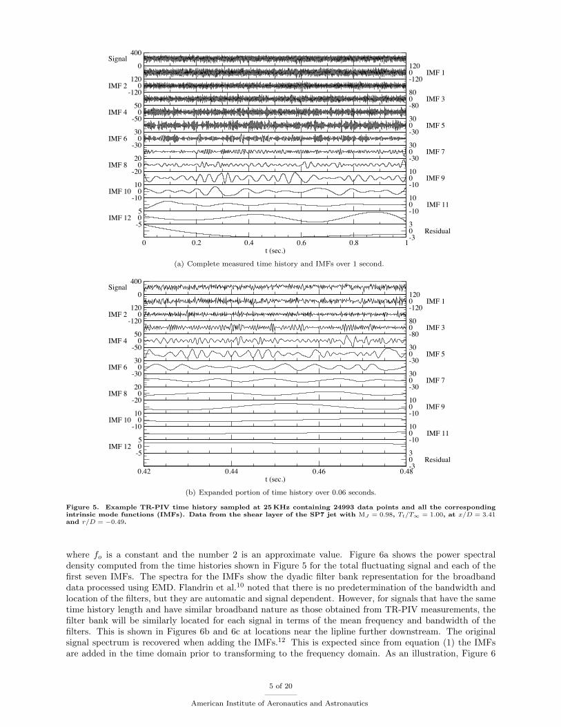
An example result of EMD performed on a TR-PIV time history is shown in Figure 5a. The total axialvelocity (mean plus fluctuating) is shown as the top signal time history. Prior to performing EMD in thisstudy, the total signal mean value was subtracted from the signal. The first process of removing the localoscillations from the local trend results in the first IMF containing the highest frequency content of thesignal. As can be observed, each succeeding IMF contains lower frequency content as the local wavelengthbetween zero crossings in the IMF increases. The residual is near zero since the total signal mean valuewas removed. Figure 5b shows the IMFs in greater detail over a fraction of the original signal length. TheIMFs for a single time history are found to be nearly orthogonal4 and uncorrelated. Further details andillustrations are given in Appendix A.

The EMD method was developed in general for non-stationary and nonlinear signals and is often appliedto signals with significant underlying trends or with short term events. Turbulence measurements suchas those presented herein are broadband and approximately stationary in nature though they representnonlinear behavior in the flow. Flandrin et al.10 and Wu & Huang11 discuss the application of EMD tobroadband signals. The decomposition of a broadband signal into N IMFs gives a result that representsa signal having been processed by a dyadic filter bank with N filters. A dyadic filter bank is a set ofoverlapping, band-pass-type filters having a constant band-pass shape with each filter having half or doublethe frequency range of its neighboring filters. The mean frequencies of the filter bank are given by

f cn = fo 2−n (2)

4 of 20


0

400Signal

-1200120

IMF 1

-1200

120IMF 2

-80080

IMF 3

-500

50IMF 4

-30030

IMF 5

-300

30IMF 6

-30030

IMF 7

-200

20IMF 8

-10010

IMF 9

-100

10IMF 10

-10010

IMF 11

-505

IMF 12

0 0.2 0.4 0.6 0.8 1t (sec.)

-303

Residual

(a) Complete measured time history and IMFs over 1 second.

0

400Signal

-1200120

IMF 1

-1200

120IMF 2

-80080

IMF 3

-500

50IMF 4

-30030

IMF 5

-300

30IMF 6

-30030

IMF 7

-200

20IMF 8

-10010

IMF 9

-100

10IMF 10

-10010

IMF 11

-505

IMF 12

0.42 0.44 0.46 0.48t (sec.)

-303

Residual

(b) Expanded portion of time history over 0.06 seconds.

Figure 5. Example TR-PIV time history sampled at 25 KHz containing 24993 data points and all the correspondingintrinsic mode functions (IMFs). Data from the shear layer of the SP7 jet with MJ = 0.98, Tt/T∞ = 1.00, at x/D = 3.41and r/D = −0.49.

where fo is a constant and the number 2 is an approximate value. Figure 6a shows the power spectraldensity computed from the time histories shown in Figure 5 for the total fluctuating signal and each of thefirst seven IMFs. The spectra for the IMFs show the dyadic filter bank representation for the broadbanddata processed using EMD. Flandrin et al.10 noted that there is no predetermination of the bandwidth andlocation of the filters, but they are automatic and signal dependent. However, for signals that have the sametime history length and have similar broadband nature as those obtained from TR-PIV measurements, thefilter bank will be similarly located for each signal in terms of the mean frequency and bandwidth of thefilters. This is shown in Figures 6b and 6c at locations near the lipline further downstream. The originalsignal spectrum is recovered when adding the IMFs.12 This is expected since from equation (1) the IMFsare added in the time domain prior to transforming to the frequency domain. As an illustration, Figure 6

5 of 20


shows the spectra computed after summing IMFs 2 and 3. The spectral level of the total fluctuating velocityis nearly recovered in this region of the spectrum.

fD/UJ

Pow

er S

pect

ral D

ensi

ty

10-2 10-1 100

10-3

10-2

10-1

1

23456

7

(a) x/D = 3.41 and r/D = −0.49

fD/UJ

Pow

er S

pect

ral D

ensi

ty

10-2 10-1 100

10-3

10-2

10-1

1

2345

6

7

(b) x/D = 7.82 and r/D = −0.49

fD/UJ

Pow

er S

pect

ral D

ensi

ty

10-2 10-1 100

10-3

10-2

10-1

1

2

3456

7

(c) x/D = 10.0 and r/D = −0.49

Figure 6. Power spectral densities computed for the axial velocity fluctuations at 3 axial locations near the jet lipline.SP7 jet with MJ = 0.98 and Tt/T∞ = 1.00. Highest levels are the total fluctuating velocity spectra. Intrinsic modefunction (IMF) spectra are labelled 1 to 7. Dashed lines are spectra for the sum of IMFs 2 and 3.

IV. Correlation Definitions

The data from TR-PIV is arranged as an array of time histories located at discrete points in a planethat cuts across the flow field of the jet. These data may be used to compute both second- and fourth-order,two-point correlations of the velocity fluctuations both for the total fluctuation and for the IMF components.However, the 1 second time histories were too short to obtain sufficient averages for reliable fourth-ordercorrelations. Thus, this paper concentrates on computing second-order correlations. The second-order,two-point correlation is defined over a time length T by

Rij(x,η, τ) =1

T

∫ T0

u′i(x, t)u′j(x+ η, t+ τ) dt (3)

where u′i(x, t) is the total fluctuating velocity (given that the fluctuating velocity is a sum of IMF components)

in the i-th direction obtained from the total velocity using u′i(x, t) = ui(x, t) − ui(x, t), η is the spatialseparation, τ is the time delay, and an overbar denotes the time average of the quantity. (From hereon,the term ‘total’ refers to the total fluctuating velocity.) The normalized two-point correlation or correlation

6 of 20


coefficient is given by

rij(x,η, τ) =Rij(x,η, τ)[

1T∫ T0u′i(x, t)u

′i(x, t) dt 1

T∫ T0u′j(x+ η, t+ τ)u′j(x+ η, t+ τ) dt

]1/2 (4)

where the denominator integrals are the mean square values of the velocity fluctuations at the two locationsin the field.

Generalizing equation (1) for different fluctuating velocity components at each point in space

u′i(x, t) =

N∑n=1

Cin(x, t) + ziN (x, t) , (5)

we substitute this into equation (3) and multiply the terms to get the correlation equation that applies afterempirical mode decomposition.

Rij(x,η, τ) =

N∑n=1

1

T

∫ T0

Cin(x, t)Cjn(x+ η, t+ τ) dt+

N∑n=1

1

T

∫ T0

Cin(x, t)

N∑k 6=n

Cjk(x+ η, t+ τ) dt

+

N∑n=1

1

T

∫ T0

ziN (x, t)Cjn(x+ η, t+ τ) dt+

N∑n=1

1

T

∫ T0

Cin(x, t)zjN (x+ η, t+ τ) dt

+1

T

∫ T0

ziN (x, t)zjN (x+ η, t+ τ) dt (6)

This equation is also normalized as in equation (4), thus all the normalized correlations involving the IMFsare relative to the root mean square values of the total fluctuating velocities at the two locations.

To compute the length and time scales from the normalized, two-point correlation, we follow the approachof Kerherve et al.13 The integral length scale is computed from

Λkij(x) =

∫ +∞

0

rij(x, ηk, τ = 0) dηk (7)

and the integral time scale by

τkij(x) =

∫ +∞

0

rij(x, ηk = Uckτ, τ) dτ (8)

where Uck is the phase speed in the ηk direction. These scales are determined for signals that either containedall the frequency content of the total fluctuating velocity or the band-pass frequency content of the individualIMFs. To determine the frequency dependence of these scales, Kerherve et al.13 used the complex coherencefunction. This function is computed using the Fourier transform with respect to the time delay of equation(3), the cross-power spectral density function, and the Fourier transforms of the velocity correlations at thetwo points in the field. See Kerherve et al.13 for the details. The final results for the frequency dependentlength scale and the frequency dependent time scale are

Λkij(x, ω) =

∫ +∞

0

<{γij(x, ηk, ω)} dηk (9)

and

τkij(x, ω) =1

uck(ω)

∫ +∞

0

|γij(x, ηk, ω)| dηk (10)

where, following Morris & Zaman,14

uck(ω) = ω/|∂φ(ηk, ω)/∂ηk|, (11)

γij is the complex coherence function, < denotes the real part, and φ(ηk, ω) is the phase of the complexcoherence function.

7 of 20


The approximately 1 second of data obtained from the TR-PIV measurements provided time historiescontaining 24993 samples. The calculation of the correlations and spectra were performed following pro-cedures given in Bendat & Piersol.15 The time histories were divided into equal length segments. Eachsegment was windowed using a Kaiser-Bessel window (parameter α = 3.0), zero padded, and then processedby the fast Fourier transform. The segment transforms were summed and averaged to obtain auto- andcross-spectra. These were then inverse Fourier transformed to obtain the auto- and cross-correlations. Witha fixed time history length, a trade-off has to be made between good frequency resolution and low variance.16

For this study, the time histories were divided into 194 segments with 256 points each with 50% overlap.This resulted in a frequency resolution of 48.8 Hz for spectrum estimates with a standard deviation of 8%.

V. Results

The velocity time histories at each point in the frame of TR-PIV data are decomposed into IMFs thatare used to compute the second-order, two-point correlation of equation (6) normalized as in equation (4).The last three terms in equation (6) are correlations involving the residual of the decomposition. Figure 5shows the residual to be relatively small and nearly constant compared to most IMFs. Consequently, theintegral involving residuals is small and the integrals involving residuals and IMFs are nearly zero. Thelatter follows from removing the nearly constant residual from the integral resulting in a computation of theaverage intrinsic mode value which is zero. Of the remaining two integrals, we will concentrate in this paperon computing the first integral; the second-order, two-point correlation of IMFs of the same mode number.

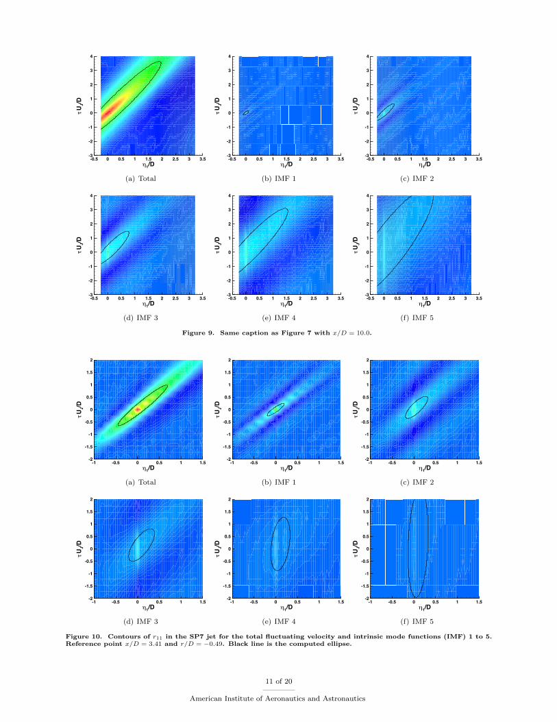
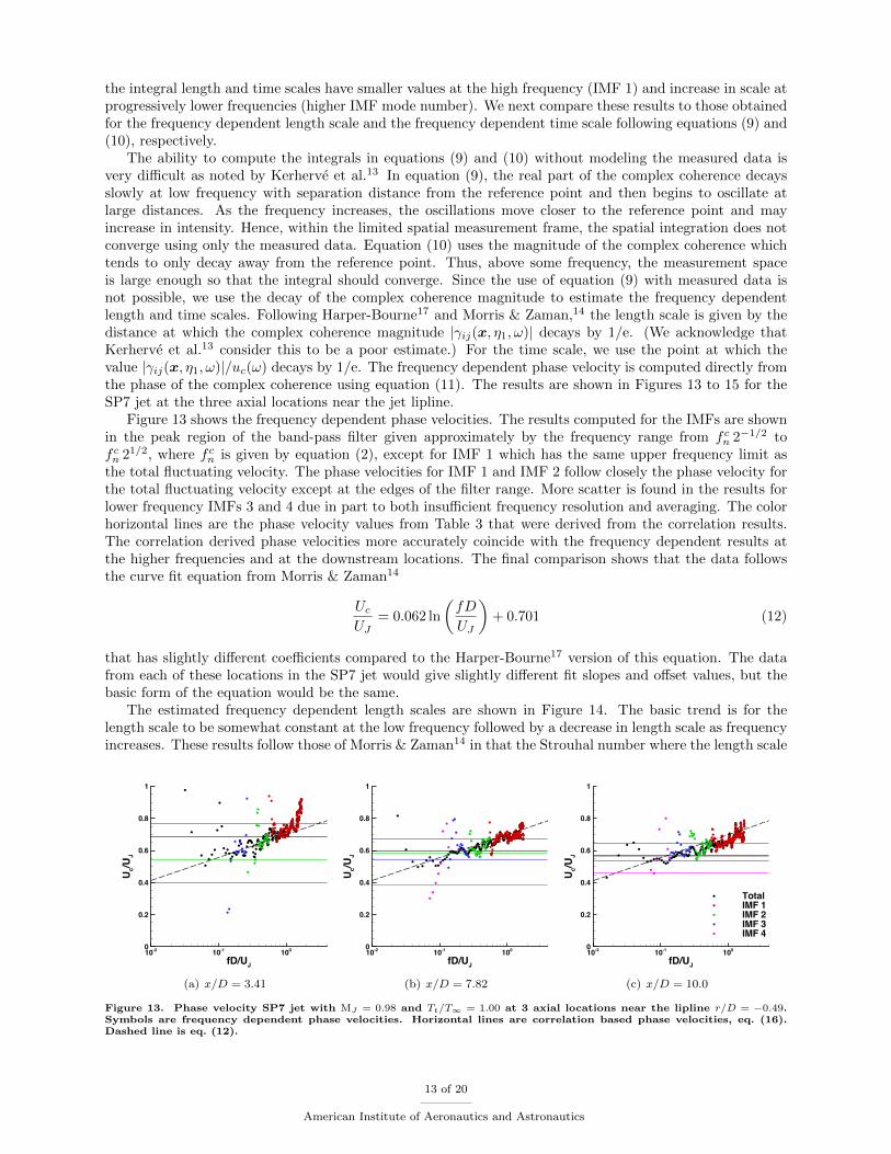
Contour plots of r11(x, η1, τ), the correlation between fluctuating axial velocity components, are shownin Figures 7 to 12 for the total fluctuating axial velocity and the first 5 IMFs from the two jets listed inTable 1 at the three reference points. The correlations are shown as a function of the normalized axialseparation η1/D and the normalized delay time τUJ/D. All the correlation plots are on the same contourscale from -0.1 to 1.0, thus the IMF correlation levels are relative to the total fluctuating velocity correlationlevel. A computed elliptic contour is included in the figures. These will be defined in the next paragraph.The IMF correlations all follow the same pattern. The highest frequency intrinsic mode IMF 1 is confinedto a small region of space and time. As the frequency decreases with increasing IMF mode number, thecorrelation broadens in both space and time. There is also a noticeable change in the slope of the contourswith IMF indicating a change in phase velocity with frequency. Two issues affect the results obtained fromthese correlations. The first is a lack of spatial grid points to properly resolve the rapid changes in thecorrelations in the high frequency IMF 1, especially in the lower velocity SP3 jet. The second is manifestas an anomaly visible in the contour plots at η1/D = 0 and centered on τUJ/D = 0. It is especially visiblein the generally lower contour levels in the higher number IMFs. It occurs within plus or minus one spatialgrid point of η1/D = 0. Some results were affected by this as discussed below.

To extract phase velocity and scale values from the correlation results, we fit an ellipse to a contourof the data,3 shown as the black line shape in Figures 7 to 12. The contour chosen was 1/e times thecorrelation peak r11(x, 0, 0) for the total fluctuating axial velocity or the individual IMFs. Assuming thecorrelation is monotonically decreasing, such as an exponential or Gaussian shaped function, an estimate forthe integral length scale, Lη = Λ1

11, following equation (7), was found. The distance is from the referencepoint, the origin in the (η1/D, τUJ/D) plane, to the ellipse along η1/D at τUJ/D = 0. Similarly, the integraltime scale, τη = τ111, equation (8), was estimated using the distance from the reference point to the ellipsealong the line η1/D = (Uc/UJ)(τUJ/D). The phase velocity Uc/UJ was also determined from the ellipseequation. The details of this ellipse method are given in Appendix B. An advantage of this method is thatit allows scale estimates to be made where measured data is lacking. For example, Figure 11a shows thatthe reference point is too close to the downstream edge of the measurement frame to allow the correlationto decay sufficiently along the constant phase velocity line to obtain an estimate for the integral time scale.However, with the ellipse equation determined from fitting the available data, an estimate for the time scalecan be computed. The results using this method to estimate the phase velocities and the integral lengthand time scales are shown in Table 2 for the SP3 jet and in Table 3 for the SP7 jet. For reference, themean axial velocities at the reference points are included in the tables. The values missing in the tablesare due to the ellipse method giving unreliable results. Especially at the shear layer reference point and forhigher number IMFs, the presence of the anomaly affects the location of the ellipse fitting points, skewingthe tilt of the ellipse and affecting the length of the ellipse axes. Thus, the extracted values based on theellipse method were inaccurate. As a check of the method in general, we compare the total fluctuating

8 of 20


x/D Total IMF 1 IMF 2 IMF 3 IMF 4 u/UJ

2.39 Uc/UJ 0.705 – – – – 0.756

Lη/D 0.108 – – – –

τηUJ/D 0.408 – – – –

6.90 Uc/UJ 0.564 0.709 0.580 0.550 0.478 0.594

Lη/D 0.388 0.061 0.137 0.287 0.509

τηUJ/D 3.148 0.135 0.567 1.686 2.633

10.0 Uc/UJ 0.529 0.623 0.541 0.498 0.480 0.548

Lη/D 0.459 0.064 0.144 0.299 0.529

τηUJ/D 3.638 0.142 0.655 1.480 3.089

Table 2. Integral properties from correlations for the total fluctuating velocity and IMF components at three axiallocations near the lipline r/D = −0.49 using the ellipse method. SP3 jet. Phase velocity, Uc. Integral length scale, Lη.Integral time scale, τη. Mean axial velocity, u.

velocity results in Table 3 for the SP7, cold, MJ = 0.9 jet to those values found by Kerherve et al.13 for anisothermal, MJ = 0.9 jet on the lipline near the end of the potential core. Using Table 3 at x/D = 7.82,we get Uc = 185 m/s, Lη = 18.6 mm, and τη = 0.50 ms. The Kerherve et al.13 values are Uc = 137 m/s,Lη = 19 mm, and τη = 0.62 ms. These results show that the ellipse method can produce correlation-basedphase velocity and scale values comparable with other methods. The assumption here is that the correlationin this part of the flow follows an exponential or Gaussian shape implying little or no significant oscillationsin the tail of the correlation.

Within the limitations of the frequency range of the measurements and the nature of empirical modedecomposition, the IMF 1 values in Tables 2 and 3 represent the measured small-scale turbulent phasevelocity and integral scales. Though the comparison is qualitative, since the measurements here are nearthe lipline of an axisymmetric jet, a couple of trends are similar to those found by Bodony & Lele3 from thecomputed results for a two-dimensional shear layer. One is that the total turbulence phase velocities are lessthan the mean velocities on the higher-speed side of the shear layer and that the small-scale phase velocitiesmay be higher (and in this case are higher) than the total phase velocities. The other is that the small-scaleintegral scales are much smaller than the total fluctuating velocity integral scales. The computed shear layersmall-scale integral scales are 60 to 80% smaller in the downstream portion of the shear layer. For the twojet cases here, the small-scale integral scales are 80 to 95% smaller.

Given that the intrinsic mode functions isolate a range of frequencies that decrease in frequency as theIMF mode number increases, the turbulent phase velocity and scale values listed in Tables 2 and 3 show thegross changes in these values with frequency. The phase velocity decreases with decreasing frequency and

x/D Total IMF 1 IMF 2 IMF 3 IMF 4 u/UJ

3.41 Uc/UJ 0.687 0.769 0.540 0.396 – 0.747

Lη/D 0.162 0.090 0.172 0.252 –

τηUJ/D 0.984 0.245 0.529 0.807 –

7.82 Uc/UJ 0.596 0.670 0.586 0.540 0.384 0.626

Lη/D 0.366 0.076 0.206 0.375 0.545

τηUJ/D 3.057 0.403 1.036 2.246 2.266

10.0 Uc/UJ 0.568 0.644 0.562 0.535 0.460 0.592

Lη/D 0.433 0.090 0.215 0.401 0.684

τηUJ/D 3.606 0.280 1.089 2.314 3.476

Table 3. Integral properties from correlations for the total fluctuating velocity and IMF components at three axiallocations near the lipline r/D = −0.49 using the ellipse method. SP7 jet. Phase velocity, Uc. Integral length scale, Lη.Integral time scale, τη. Mean axial velocity, u.

9 of 20


1/D

UJ/D

-0.5 0 0.5 1 1.5-1

-0.5

0

0.5

1

1.5

2

(a) Total

1/D

UJ/D

-0.5 0 0.5 1 1.5-1

-0.5

0

0.5

1

1.5

2

(b) IMF 1

1/D

UJ/D

-0.5 0 0.5 1 1.5-1

-0.5

0

0.5

1

1.5

2

(c) IMF 2

1/D

UJ/D

-0.5 0 0.5 1 1.5-1

-0.5

0

0.5

1

1.5

2

(d) IMF 3

1/D

UJ/D

-0.5 0 0.5 1 1.5-1

-0.5

0

0.5

1

1.5

2

(e) IMF 4

1/D

UJ/D

-0.5 0 0.5 1 1.5-1

-0.5

0

0.5

1

1.5

2

(f) IMF 5

Figure 7. Contours of r11 in the SP3 jet for the total fluctuating velocity and intrinsic mode functions (IMF) 1 to 5.Reference point x/D = 2.39 and r/D = −0.49. Black line is the computed ellipse.

1/D

UJ/D

-1 -0.5 0 0.5 1 1.5 2-3

-2

-1

0

1

2

3

4

(a) Total

1/D

UJ/D

-1 -0.5 0 0.5 1 1.5 2-3

-2

-1

0

1

2

3

4

(b) IMF 1

1/D

UJ/D

-1 -0.5 0 0.5 1 1.5 2-3

-2

-1

0

1

2

3

4

(c) IMF 2

1/D

UJ/D

-1 -0.5 0 0.5 1 1.5 2-3

-2

-1

0

1

2

3

4

(d) IMF 3

1/D

UJ/D

-1 -0.5 0 0.5 1 1.5 2-3

-2

-1

0

1

2

3

4

(e) IMF 4

1/D

UJ/D

-1 -0.5 0 0.5 1 1.5 2-3

-2

-1

0

1

2

3

4

(f) IMF 5

Figure 8. Same caption as Figure 7 with x/D = 6.90.

10 of 20


1/D

UJ/D

-0.5 0 0.5 1 1.5 2 2.5 3 3.5-3

-2

-1

0

1

2

3

4

(a) Total

1/D

UJ/D

-0.5 0 0.5 1 1.5 2 2.5 3 3.5-3

-2

-1

0

1

2

3

4

(b) IMF 1

1/D

UJ/D

-0.5 0 0.5 1 1.5 2 2.5 3 3.5-3

-2

-1

0

1

2

3

4

(c) IMF 2

1/D

UJ/D

-0.5 0 0.5 1 1.5 2 2.5 3 3.5-3

-2

-1

0

1

2

3

4

(d) IMF 3

1/D

UJ/D

-0.5 0 0.5 1 1.5 2 2.5 3 3.5-3

-2

-1

0

1

2

3

4

(e) IMF 4

1/D

UJ/D

-0.5 0 0.5 1 1.5 2 2.5 3 3.5-3

-2

-1

0

1

2

3

4

(f) IMF 5


1/D

UJ/D

-1 -0.5 0 0.5 1 1.5-2

-1.5

-1

-0.5

0

0.5

1

1.5

2

(a) Total

1/D

UJ/D

-1 -0.5 0 0.5 1 1.5-2

-1.5

-1

-0.5

0

0.5

1

1.5

2

(b) IMF 1

1/D

UJ/D

-1 -0.5 0 0.5 1 1.5-2

-1.5

-1

-0.5

0

0.5

1

1.5

2

(c) IMF 2

1/D

UJ/D

-1 -0.5 0 0.5 1 1.5-2

-1.5

-1

-0.5

0

0.5

1

1.5

2

(d) IMF 3

1/D

UJ/D

-1 -0.5 0 0.5 1 1.5-2

-1.5

-1

-0.5

0

0.5

1

1.5

2

(e) IMF 4

1/D

UJ/D

-1 -0.5 0 0.5 1 1.5-2

-1.5

-1

-0.5

0

0.5

1

1.5

2

(f) IMF 5

Figure 10. Contours of r11 in the SP7 jet for the total fluctuating velocity and intrinsic mode functions (IMF) 1 to 5.Reference point x/D = 3.41 and r/D = −0.49. Black line is the computed ellipse.

11 of 20


1/D

UJ/D

-2 -1.5 -1 -0.5 0 0.5 1 1.5-4

-3

-2

-1

0

1

2

3

4

(a) Total

1/D

UJ/D

-2 -1.5 -1 -0.5 0 0.5 1 1.5-4

-3

-2

-1

0

1

2

3

4

(b) IMF 1

1/D

UJ/D

-2 -1.5 -1 -0.5 0 0.5 1 1.5-4

-3

-2

-1

0

1

2

3

4

(c) IMF 2

1/D

UJ/D

-2 -1.5 -1 -0.5 0 0.5 1 1.5-4

-3

-2

-1

0

1

2

3

4

(d) IMF 3

1/D

UJ/D

-2 -1.5 -1 -0.5 0 0.5 1 1.5-4

-3

-2

-1

0

1

2

3

4

(e) IMF 4

1/D

UJ/D

-2 -1.5 -1 -0.5 0 0.5 1 1.5-4

-3

-2

-1

0

1

2

3

4

(f) IMF 5


1/D

UJ/D

-0.5 0 0.5 1 1.5 2 2.5 3 3.5-3

-2

-1

0

1

2

3

4

(a) Total

1/D

UJ/D

-0.5 0 0.5 1 1.5 2 2.5 3 3.5-3

-2

-1

0

1

2

3

4

(b) IMF 1

1/D

UJ/D

-0.5 0 0.5 1 1.5 2 2.5 3 3.5-3

-2

-1

0

1

2

3

4

(c) IMF 2

1/D

UJ/D

-0.5 0 0.5 1 1.5 2 2.5 3 3.5-3

-2

-1

0

1

2

3

4

(d) IMF 3

1/D

UJ/D

-0.5 0 0.5 1 1.5 2 2.5 3 3.5-3

-2

-1

0

1

2

3

4

(e) IMF 4

1/D

UJ/D

-0.5 0 0.5 1 1.5 2 2.5 3 3.5-3

-2

-1

0

1

2

3

4

(f) IMF 5


12 of 20


the integral length and time scales have smaller values at the high frequency (IMF 1) and increase in scale atprogressively lower frequencies (higher IMF mode number). We next compare these results to those obtainedfor the frequency dependent length scale and the frequency dependent time scale following equations (9) and(10), respectively.

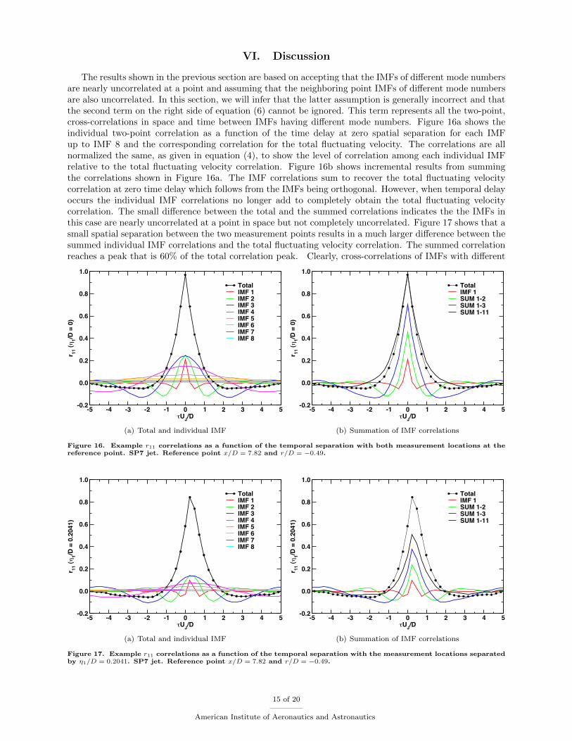
The ability to compute the integrals in equations (9) and (10) without modeling the measured data isvery difficult as noted by Kerherve et al.13 In equation (9), the real part of the complex coherence decaysslowly at low frequency with separation distance from the reference point and then begins to oscillate atlarge distances. As the frequency increases, the oscillations move closer to the reference point and mayincrease in intensity. Hence, within the limited spatial measurement frame, the spatial integration does notconverge using only the measured data. Equation (10) uses the magnitude of the complex coherence whichtends to only decay away from the reference point. Thus, above some frequency, the measurement spaceis large enough so that the integral should converge. Since the use of equation (9) with measured data isnot possible, we use the decay of the complex coherence magnitude to estimate the frequency dependentlength and time scales. Following Harper-Bourne17 and Morris & Zaman,14 the length scale is given by thedistance at which the complex coherence magnitude |γij(x, η1, ω)| decays by 1/e. (We acknowledge thatKerherve et al.13 consider this to be a poor estimate.) For the time scale, we use the point at which thevalue |γij(x, η1, ω)|/uc(ω) decays by 1/e. The frequency dependent phase velocity is computed directly fromthe phase of the complex coherence using equation (11). The results are shown in Figures 13 to 15 for theSP7 jet at the three axial locations near the jet lipline.

Figure 13 shows the frequency dependent phase velocities. The results computed for the IMFs are shownin the peak region of the band-pass filter given approximately by the frequency range from f cn 2−1/2 tof cn 21/2, where f cn is given by equation (2), except for IMF 1 which has the same upper frequency limit asthe total fluctuating velocity. The phase velocities for IMF 1 and IMF 2 follow closely the phase velocity forthe total fluctuating velocity except at the edges of the filter range. More scatter is found in the results forlower frequency IMFs 3 and 4 due in part to both insufficient frequency resolution and averaging. The colorhorizontal lines are the phase velocity values from Table 3 that were derived from the correlation results.The correlation derived phase velocities more accurately coincide with the frequency dependent results atthe higher frequencies and at the downstream locations. The final comparison shows that the data followsthe curve fit equation from Morris & Zaman14

UcUJ

= 0.062 ln

(fD

UJ

)+ 0.701 (12)

that has slightly different coefficients compared to the Harper-Bourne17 version of this equation. The datafrom each of these locations in the SP7 jet would give slightly different fit slopes and offset values, but thebasic form of the equation would be the same.

The estimated frequency dependent length scales are shown in Figure 14. The basic trend is for thelength scale to be somewhat constant at the low frequency followed by a decrease in length scale as frequencyincreases. These results follow those of Morris & Zaman14 in that the Strouhal number where the length scale

fD/UJ

Uc/U

J

10-2 10-1 1000

0.2

0.4

0.6

0.8

1

(a) x/D = 3.41

fD/UJ

Uc/U

J

10-2 10-1 1000

0.2

0.4

0.6

0.8

1

(b) x/D = 7.82

fD/UJ

Uc/U

J

10-2 10-1 1000

0.2

0.4

0.6

0.8

1

TotalIMF 1IMF 2IMF 3IMF 4

(c) x/D = 10.0

Figure 13. Phase velocity SP7 jet with MJ = 0.98 and Tt/T∞ = 1.00 at 3 axial locations near the lipline r/D = −0.49.Symbols are frequency dependent phase velocities. Horizontal lines are correlation based phase velocities, eq. (16).Dashed line is eq. (12).

13 of 20


fD/UJ

L/D

(Est

.)

10-2 10-1 100

10-1

100

(a) x/D = 3.41

fD/UJ

L/D

(Est

.)

10-2 10-1 100

10-1

100

(b) x/D = 7.82

fD/UJ

L/D

(Est

.)

10-2 10-1 100

10-1

100

(c) x/D = 10.0

Figure 14. Length scale SP7 jet with MJ = 0.98 and Tt/T∞ = 1.00 at 3 axial locations near the lipline r/D = −0.49.Symbols are frequency dependent length scales. Horizontal lines are correlation based integral length scales, eq. (14).See Fig. 13c for legend.

changes from constant to a decreasing value moves to a lower value as the reference point moves downstream.At the end of the potential core location shown in Figure 14b, there is insufficient axial extent to enablethe computation of the lower Strouhal number length scales. The IMF results follow those for the totalfluctuating velocity, though the estimates for the length scale are lower for IMFs 2 to 4. A possible reasonfor this will be discussed in the next section. A comparison of these results with the correlation integrallength scale (horizontal lines for the values from Table 3) may indicate that the estimates for the frequencydependent length scale are too high. The oscillations inherent in the real part of the complex coherencewould provide cancellations in the calculation of equation (9) resulting in smaller length scales that wouldcoincide more closely with the integral length scales.

Figure 15 shows the frequency dependent time scale for the total fluctuating velocity and the IMFs wherethere is sufficient data in the axial direction to make the calculation. The comparisons with the integral timescales are closer in value than found for the length scale comparison in Figure 14. Again, the IMF resultsfollow the total fluctuating velocity results with more scatter in IMFs 2 to 4 especially in the shear layer.The accuracy of computing the integral time scale using the ellipse method was estimated for the IMF 1and IMF 2 results shown in Figure 15c. The 1/e point was found by interpolation along the constant phasevelocity line of r11. The results are given by the dashed lines in the figure. For IMF 1, the directly computedintegral time scale is 33% higher than the ellipse method time scale. With better resolution at IMF 2, thedifference decreases to 11%.

fD/UJ

UJ/D

10-2 10-1 10010-1

100

101

(a) x/D = 3.41

fD/UJ

UJ/D

10-2 10-1 10010-1

100

101

(b) x/D = 7.82

fD/UJ

UJ/D

10-2 10-1 10010-1

100

101

(c) x/D = 10.0

Figure 15. Time scale SP7 jet with MJ = 0.98 and Tt/T∞ = 1.00 at 3 axial locations near the lipline r/D = −0.49.Symbols are frequency dependent time scales. Horizontal lines are correlation based integral time scales, eq. (15). SeeFig. 13c for legend.

14 of 20


VI. Discussion

The results shown in the previous section are based on accepting that the IMFs of different mode numbersare nearly uncorrelated at a point and assuming that the neighboring point IMFs of different mode numbersare also uncorrelated. In this section, we will infer that the latter assumption is generally incorrect and thatthe second term on the right side of equation (6) cannot be ignored. This term represents all the two-point,cross-correlations in space and time between IMFs having different mode numbers. Figure 16a shows theindividual two-point correlation as a function of the time delay at zero spatial separation for each IMFup to IMF 8 and the corresponding correlation for the total fluctuating velocity. The correlations are allnormalized the same, as given in equation (4), to show the level of correlation among each individual IMFrelative to the total fluctuating velocity correlation. Figure 16b shows incremental results from summingthe correlations shown in Figure 16a. The IMF correlations sum to recover the total fluctuating velocitycorrelation at zero time delay which follows from the IMFs being orthogonal. However, when temporal delayoccurs the individual IMF correlations no longer add to completely obtain the total fluctuating velocitycorrelation. The small difference between the total and the summed correlations indicates the the IMFs inthis case are nearly uncorrelated at a point in space but not completely uncorrelated. Figure 17 shows that asmall spatial separation between the two measurement points results in a much larger difference between thesummed individual IMF correlations and the total fluctuating velocity correlation. The summed correlationreaches a peak that is 60% of the total correlation peak. Clearly, cross-correlations of IMFs with different

-5 -4 -3 -2 -1 0 1 2 3 4 5UJ/D

-0.2

0.0

0.2

0.4

0.6

0.8

1.0

r 11 (

1/D =

0)

TotalIMF 1IMF 2IMF 3IMF 4IMF 5IMF 6IMF 7IMF 8

(a) Total and individual IMF

-5 -4 -3 -2 -1 0 1 2 3 4 5UJ/D

-0.2

0.0

0.2

0.4

0.6

0.8

1.0

r 11 (

1/D =

0)

TotalIMF 1SUM 1-2SUM 1-3SUM 1-11

(b) Summation of IMF correlations

Figure 16. Example r11 correlations as a function of the temporal separation with both measurement locations at thereference point. SP7 jet. Reference point x/D = 7.82 and r/D = −0.49.

-5 -4 -3 -2 -1 0 1 2 3 4 5UJ/D

-0.2

0.0

0.2

0.4

0.6

0.8

1.0

r 11 (

1/D =

0.2

041)



-5 -4 -3 -2 -1 0 1 2 3 4 5UJ/D

-0.2

0.0

0.2

0.4

0.6

0.8

1.0

r 11 (

1/D =

0.2

041)



Figure 17. Example r11 correlations as a function of the temporal separation with the measurement locations separatedby η1/D = 0.2041. SP7 jet. Reference point x/D = 7.82 and r/D = −0.49.

15 of 20


mode numbers are required to make up the difference. Further examples of correlations as a function of theaxial spatial separation are shown in Figure 18 for zero time delay and in Figure 19 for a small time delaybetween measurement points. The requirement for including IMF cross-correlation terms is clearly evidentas the sum of the individual IMF correlations falls short of the total fluctuating velocity correlation.

The consequence of neglecting the cross-correlations between IMFs of different mode numbers can alsobe found in the phase velocity and scale results in Figures 13 to 15. For IMF 1, the effects appear to besmall in the range of Strouhal number 1 to 2, the upper half of the measured frequency range. The totalfluctuating velocity and IMF 1 results are in basic agreement. The IMF cross-correlation terms are notas important for the IMF 1 results except near the lower end of the frequency range. The IMF 2 to 4results occur in increasingly narrower frequency bands resulting in deviations in the phase velocities anddecreases in the length and time scales compared to the total fluctuating velocity results. In Figure 14,the frequency dependent length scales of IMFs 2 to 4 are smaller than the corresponding length scales forthe total fluctuating velocity. The difference comes from the neglected cross-correlation terms that passthrough the linear process of Fourier transforming equation (6) and taking the real part in equation (9). Thedifferences in the frequency dependent time scales are more difficult to discern since taking the magnitudeof the complex coherence function, equation (10), is not a linear process.

-2 -1 0 11/D

-0.2

0.0

0.2

0.4

0.6

0.8

1.0

r 11 (

UJ/D

= 0

)



-2 -1 0 11/D

-0.2

0.0

0.2

0.4

0.6

0.8

1.0

r 11 (

UJ/D

= 0

)



Figure 18. Example r11 correlations as a function of the axial spatial separation with no time delay between measurementlocations. SP7 jet. Reference point x/D = 7.82 and r/D = −0.49.

-2 -1 0 11/D

-0.2

0.0

0.2

0.4

0.6

0.8

1.0

r 11 (

UJ/D

= 0

.976

4)



-2 -1 0 11/D

-0.2

0.0

0.2

0.4

0.6

0.8

1.0

r 11 (

UJ/D

= 0

.976

4)



Figure 19. Example r11 correlations as a function of the axial spatial separation with a time delay of τUJ/D = 0.9764between measurement locations. SP7 jet. Reference point x/D = 7.82 and r/D = −0.49.

16 of 20


VII. Concluding Remarks

A new application of the empirical mode decomposition (EMD) method has been shown in this paper.Instead of analyzing a single time history signal or a small set of time histories, a large array of closelyspaced time histories derived from TR-PIV measurements have been analyzed. The results from EMD wereequivalent to passing the time histories through a bank of band-pass filters. This data was then used intwo-point correlation calculations resulting in the determination of turbulence phase velocities and lengthand time scales that only apply to a particular band-pass range. The highest frequency-range results maybe applicable to subgrid scale noise source modeling.

Some issues were identified that would need to be resolved to better use the method.

• A higher sampling rate would increase the Strouhal number range that can be analyzed and/or allowhigher speed jets to be studied.

• The length of the time histories needs to be increased. This would allow for greater frequency resolutionand/or allow a larger number of averages to be performed to reduce spectral variance and allow betterresults for fourth-order correlation calculations.

• There needs to be finer spatial resolution in the TR-PIV measurements. The higher frequency corre-lations can change rapidly in a short distance.

Unfortunately, hardware limitations may inhibit significant improvements in any of these issues.Finally, there is the issue of the importance of the cross-correlation of IMFs of different mode numbers.

Since the IMFs represent data in overlapping frequency bands, it is not yet known if these space-time cross-correlations are between different frequency data or between the same frequencies in the overlapping regions.The fact that the highest frequency IMF 1 results appeared not to deviate much from the total results exceptat the low end of the frequency range suggests the latter explanation for the results. The lower frequencyIMFs have overlap on both ends of the band-pass filter with results showing that the cross-correlationinformation is missing. Resolving these matters is part of future work.

Appendix A – Some Details of Empirical Mode Decomposition

Further details about the empirical mode decomposition (EMD) method as applied in this study aregiven in this appendix. Specifically, information is given about interpolation and sifting, stopping criteria,and boundary conditions that were used in the current work. Any issues related to these are discussed inthe references cited below

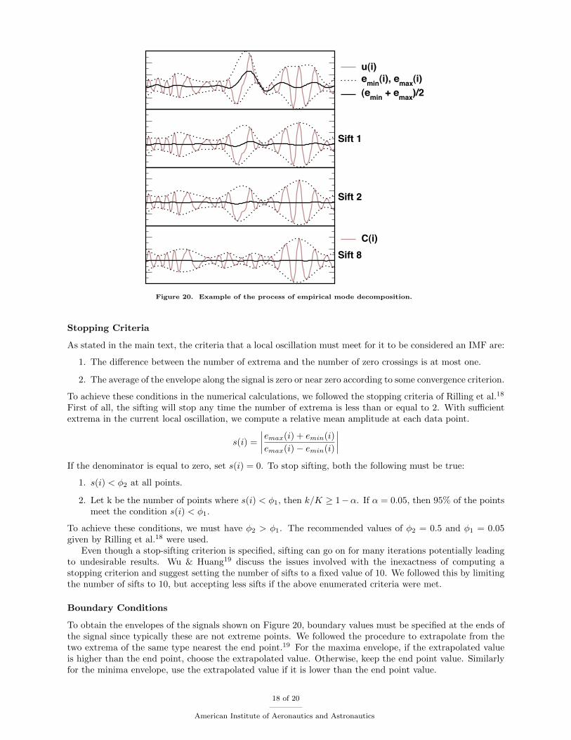
Empirical Mode Decomposition

The EMD method may be applied to any general, non-stationary, and nonlinear signal.4 The signal u(t)is sampled to create a set u(i) where i = 1, 2, . . . ,K. We start by identifying the extrema of u(i), thepositive peaks and the negative peaks in our case since the mean value of the signal is removed from thesignal prior to decomposition. The positive peaks are used to construct an interpolating function emax(i)using a cubic spline. Similarly, the negative peaks are used to construct the interpolating function emin(i).The original signal u(i) and emax(i) and emin(i) are illustrated in the top part of Figure 20. As can beseen, the interpolating functions represent the envelope of the signal u(i). We now compute the average ofthe envelope m(i) = (emax(i) + emin(i))/2, which gives the local trend in the signal. Subtracting the localtrend from the signal results in the local oscillation. Ideally, the local oscillation is a simple function withvarying amplitude and frequency with zero mean value and with the number of extrema and the number ofzero crossings differing by no more than one, called an intrinsic mode function (IMF). However in practice,these conditions do not immediately occur and a process of iteration called sifting is followed. The currentlocal oscillation becomes the new signal for which new envelope functions are determined, labelled ‘Sift 1’ inFigure 20, and the average of the envelope is computed. This new local trend is subtracted from the currentsignal to obtain the new local oscillation. As noted in the figure, at least 8 siftings are required for the localtrend to approach zero and the resulting IMF C(i) to have zero mean. It should also be noted that theenvelope of the IMF is approximately symmetric about the axis.

17 of 20


u(i)emin(i), emax(i) (emin + emax)/2

Sift 1

Sift 2

Sift 8C(i)

Figure 20. Example of the process of empirical mode decomposition.

Stopping Criteria

As stated in the main text, the criteria that a local oscillation must meet for it to be considered an IMF are:

1. The difference between the number of extrema and the number of zero crossings is at most one.

2. The average of the envelope along the signal is zero or near zero according to some convergence criterion.

To achieve these conditions in the numerical calculations, we followed the stopping criteria of Rilling et al.18

First of all, the sifting will stop any time the number of extrema is less than or equal to 2. With sufficientextrema in the current local oscillation, we compute a relative mean amplitude at each data point.

s(i) =

∣∣∣∣emax(i) + emin(i)

emax(i)− emin(i)

∣∣∣∣If the denominator is equal to zero, set s(i) = 0. To stop sifting, both the following must be true:

1. s(i) < φ2 at all points.

2. Let k be the number of points where s(i) < φ1, then k/K ≥ 1−α. If α = 0.05, then 95% of the pointsmeet the condition s(i) < φ1.

To achieve these conditions, we must have φ2 > φ1. The recommended values of φ2 = 0.5 and φ1 = 0.05given by Rilling et al.18 were used.

Even though a stop-sifting criterion is specified, sifting can go on for many iterations potentially leadingto undesirable results. Wu & Huang19 discuss the issues involved with the inexactness of computing astopping criterion and suggest setting the number of sifts to a fixed value of 10. We followed this by limitingthe number of sifts to 10, but accepting less sifts if the above enumerated criteria were met.

Boundary Conditions

To obtain the envelopes of the signals shown on Figure 20, boundary values must be specified at the ends ofthe signal since typically these are not extreme points. We followed the procedure to extrapolate from thetwo extrema of the same type nearest the end point.19 For the maxima envelope, if the extrapolated valueis higher than the end point, choose the extrapolated value. Otherwise, keep the end point value. Similarlyfor the minima envelope, use the extrapolated value if it is lower than the end point value.

18 of 20


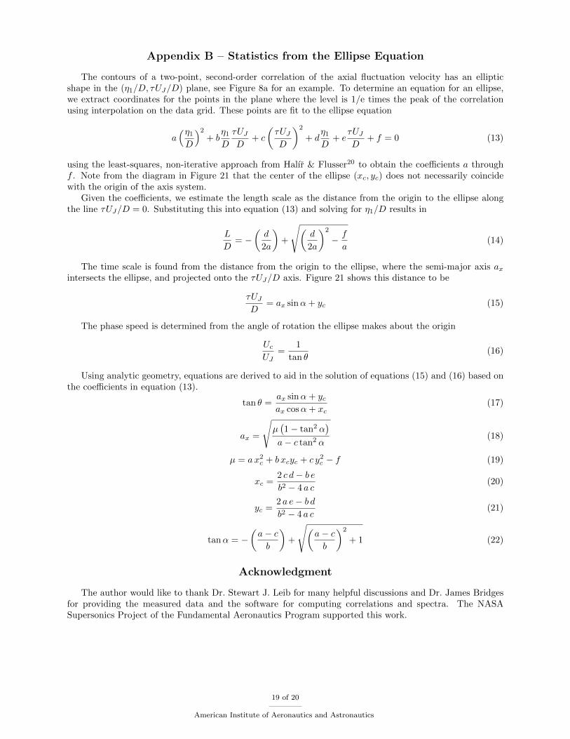
Appendix B – Statistics from the Ellipse Equation

The contours of a two-point, second-order correlation of the axial fluctuation velocity has an ellipticshape in the (η1/D, τUJ/D) plane, see Figure 8a for an example. To determine an equation for an ellipse,we extract coordinates for the points in the plane where the level is 1/e times the peak of the correlationusing interpolation on the data grid. These points are fit to the ellipse equation

a(η1D

)2+ b

η1D

τUJD

+ c

(τUJD

)2

+ dη1D

+ eτUJD

+ f = 0 (13)

using the least-squares, non-iterative approach from Halır & Flusser20 to obtain the coefficients a throughf . Note from the diagram in Figure 21 that the center of the ellipse (xc, yc) does not necessarily coincidewith the origin of the axis system.

Given the coefficients, we estimate the length scale as the distance from the origin to the ellipse alongthe line τUJ/D = 0. Substituting this into equation (13) and solving for η1/D results in

L

D= −

(d

2a

)+

√(d

2a

)2

− f

a(14)

The time scale is found from the distance from the origin to the ellipse, where the semi-major axis axintersects the ellipse, and projected onto the τUJ/D axis. Figure 21 shows this distance to be

τUJD

= ax sinα+ yc (15)

The phase speed is determined from the angle of rotation the ellipse makes about the origin

UcUJ

=1

tan θ(16)

Using analytic geometry, equations are derived to aid in the solution of equations (15) and (16) based onthe coefficients in equation (13).

tan θ =ax sinα+ ycax cosα+ xc

(17)

ax =

√µ(1− tan2 α

)a− c tan2 α

(18)

µ = a x2c + b xcyc + c y2c − f (19)

xc =2 c d− b eb2 − 4 a c

(20)

yc =2 a e− b db2 − 4 a c

(21)

tanα = −(a− cb

)+

√(a− cb

)2

+ 1 (22)

Acknowledgment

The author would like to thank Dr. Stewart J. Leib for many helpful discussions and Dr. James Bridgesfor providing the measured data and the software for computing correlations and spectra. The NASASupersonics Project of the Fundamental Aeronautics Program supported this work.

19 of 20


-0.5 0 0.5 1 1.51/D

0

1

2

3

U J/D ax

yc

xc

ax sin( )

ax cos( )

L/D

Figure 21. Diagram of ellipse system for computing phase velocity and length and time scales.

References

1Goldstein, M. E. and Leib, S. J., “The Aeroacoustics of Slowly Diverging Supersonic Jets,” J. Fluid Mech., Vol. 600,2008, pp. 291–337.

2Bodony, D. J. and Lele, S. K., “A Statistical Subgrid Scale Noise Model: Formulation,” AIAA Paper No. 2003-3252,2003.

3Bodony, D. J. and Lele, S. K., “Spatial Scale Decomposition of Shear Layer Turbulence and the Sound Sources Associatedwith the Missing Scales in a Large-Eddy Simulation,” AIAA Paper No. 2002-2454, 2002.

4Huang, N. E., Shen, Z., Long, S. R., Wu, M. C., Shih, H. H., Zheng, Q., Yen, N.-C., Tung, C. C., and Liu, H. H., “TheEmpirical Mode Decomposition and the Hilbert Spectrum for Nonlinear and Non-Stationary Time Series Analysis,” Proc. Roy.Soc. Lond. A, Vol. 454, 1998, pp. 903–995.

5Huang, N. E., Shen, Z., and Long, S. R., “A New View of Nonlinear Water Waves: The Hilbert Spectrum,” Ann. Rev.Fluid Mech., Vol. 31, 1999, pp. 417–457.

6Huang, N. E. and Wu, Z., “A Review on Hilbert-Huang Transform: Method and its Applications to Geophysical Studies,”Rev. Geophys., Vol. 46, No. RG 2006, 2008.

7Bridges, J. and Brown, C. A., “Validation of the Small Hot Jet Acoustic Rig for Aeroacoustic Research,” AIAA PaperNo. 2005-2846, 2005.

8Wernet, M. P., “Temporally Resolved PIV for Space-Time Correlations in Both Cold and Hot Jet Flows,” MeasurementScience and Technology, Vol. 18, 2007, pp. 1387–1403.

9Bridges, J. and Wernet, M. P., “Effect of Temperature on Jet Velocity Spectra,” AIAA Paper No. 2007-3628, 2007.10Flandrin, P., Rilling, G., and Goncalves, P., “Empirical Mode Decomposition as a Filter Bank,” IEEE Sig. Proc. Let.,

Vol. 11, No. 2, 2004, pp. 112–114.11Wu, Z. and Huang, N. E., “A Study of the Characteristics of White Noise using the Empirical Mode Decomposition

Method,” Proc. Roy. Soc. Lond. A, Vol. 460, 2004, pp. 1597–1611.12Huang, Y., Schmitt, F. G., Lu, Z., and Liu, Y., “Empirical Mode Decomposition Analysis of Experimental Homogeneous

Turbulence Time Series,” Colloque GRETSI 11–14 September, Troyes, France, 2007.13Kerherve, F., Fitzpatrick, J., and Jordan, P., “The Frequency Dependence of Jet Turbulence for Noise Source Modelling,”

J. Sound Vib., Vol. 296, 2006, pp. 209–225.14Morris, P. J. and Zaman, K. B. M. Q., “Velocity Measurements in Jets with Application to Noise Source Modeling,” J.

Sound Vib., Vol. 329, 2010, pp. 394–414.15Bendat, J. S. and Piersol, A. G., Random Data Analysis and Measurement Procedures, Wiley-Interscience, New York,

NY, 2nd ed., 1986.16Rabiner, L. R., Schafer, R. W., and Dlugos, D., “Periodogram Method for Power Spectrum Estimation,” Programs for

Digital Signal Processing, Section 2.1, IEEE Press, 1979, pp. 2.1–1–2.1–10.17Harper-Bourne, M., “Jet Noise Turbulence Measurements,” AIAA Paper No. 2003-3214, 2003.18Rilling, G., Flandrin, P., and Goncalves, P., “On Empirical Mode Decomposition and its Algorithms,” IEEE-EURASIP

Workshop on Nonlinear Signal and Image Processing, No. NSIP-03 Grado(I), June 2003.19Wu, Z. and Huang, N. E., “Ensemble Empirical Mode Decomposition: A Noise-Assisted Data Analysis Method,” Adv.

Adapt. Data Anal., Vol. 1, No. 1, 2009, pp. 1–41.20Halır, R. and Flusser, J., “Numerically Stable Direct Least Squares Fitting of Ellipses,” Proc. 6th Int. Conf. in Central

Europe on Computer Graphics, Visualization and Interactive Digital Media WSCG, 1998, pp. 125–132.

20 of 20


Documents

Turbulent Statistics from Time-Resolved PIV · PDF fileTurbulent Statistics from Time-Resolved PIV Measurements of a Jet Using Empirical Mode Decomposition ... -0.45-0.40-0.35 0.64