Tutorial: Analyzing real network data 1) Creating data from survey Getting Started: 1)Log into the machine (directions on board) 2)Create a directory on

Tutorial: Analyzing real network data1) Creating data from survey

Getting Started:

1) Log into the machine (directions on board)2) Create a directory on the machine you are using called “c:\Nets\”3) Go to the course webpage:http://www.soc.duke.edu/~jmoody77/SSRINets/wsfiles.htm

• Download the first 3 or 4 files and save them, including the SPAN zip file

http://www.soc.duke.edu/~jmoody77/SSRINets/wsfiles.htm


You can download all of the needed files from here:


-Outline:-From survey to analysis files-Exploring the network: visualization-Moving data among programs

-SAS, PAJEK, UCINET, R-Network Position Measures

-Centrality, Reachability, Reciprocity, Constraint, Mixing/Homophily.-Network Behavior & Peer Influence Models

-Network structure as indep variable-Peer influence models-Dyad similarity models

-Network Structure analyses-Clustering for peer groups-Block models-Statistical Models for networks (STANET).


This is what students filled out in the Add Health, in school survey. One set for male friends, another for female friends.

This is the foundation of our data….


This is what students filled out in the Add Health, in school survey. One set for male friends, another for female friends.

This is the foundation of our data….

Resulting in a nomination data file that looks something like this (actual numbers changed).

We want to turn this file into something PAJEK, UCINET, etc. can read.

Open “netcreate.sas” & walk through logic of the file.


Netcreate.sas used files from SPAN to create PAJEK files.

After reading in the data, we use an %include statement to get the needed subroutines from SPAN.


The %include statement reads in subroutines for network analysis

Tutorial: Analyzing real network data1) Creating data from survey (aside to SPAN manual!)



We first use the adj() routine to create an adjacency matrix.

Then we select just ties matching within the nominated set and then write out a set of node-level attribute files.


We can also store the main files for later use in matrix format.


The PAJEK format is a simple text file:

This is the minimum specification for a file. In addition, you can add cols in the *Vertices section to specify shape, color, xyz coords. Ditto w. arcs & edges.


*Vertices 10 1 1 2 2 3 3 4 4 5 5 6 6 7 7 8 8 9 9 10 10*Arcs 1 4 1.00 1 5 1.00 1 6 1.00 1 10 1.00 2 8 1.00 2 9 1.00 3 2 1.00 3 4 1.00 3 10 1.00 4 8 1.00 5 3 1.00 5 4 1.00 5 8 1.00 5 9 1.00 6 4 1.00 6 5 1.00 7 3 1.00 7 10 1.00 8 6 1.00 8 7 1.00 8 9 1.00 9 10 1.00 10 2 1.00*Edges 1 8 1.00 2 4 1.00 2 7 1.00 5 7 1.00 6 9 1.00

Tutorial: Analyzing real network data2) Exploring the network graphically

I think it’s useful to simply “play” with the network in various ways and get a sense of the shape of the network. This is perhaps PAJEK’s most useful purpose.

-- Load a network and work through good/bad plots, basic PAJEK interface. -- Note the diff btwn the full nomination matrix and the in-school only matrix.

Tutorial: Analyzing real network data2) Exploring the network graphically

Once you have a network, how do you create a print-ready image?

a) Screen shots (good for .ppt)b) Export to .eps or FLASH and edit in Illustrator

Tutorial: Analyzing real network data3) Basic Network Statistics

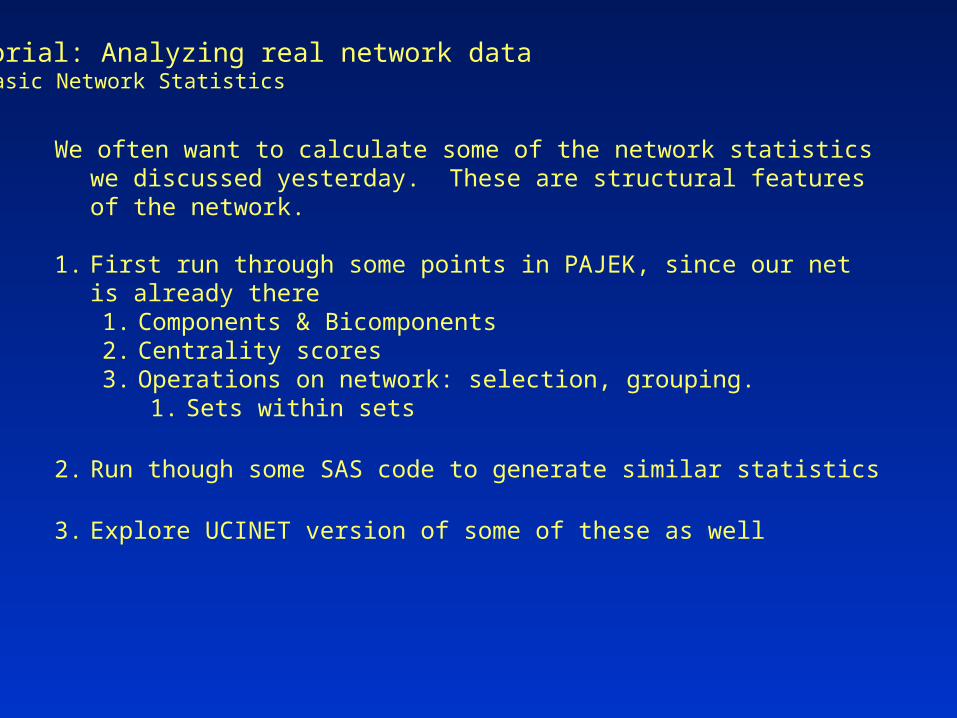
We often want to calculate some of the network statistics we discussed yesterday. These are structural features of the network.

1. First run through some points in PAJEK, since our net is already there1. Components & Bicomponents2. Centrality scores3. Operations on network: selection, grouping.

1. Sets within sets

2. Run though some SAS code to generate similar statistics

3. Explore UCINET version of some of these as well

Tutorial: Analyzing real network data3) Network Behavior & Peer Influence

Open nodestats1.sas to see how to code these same stats, plus a few, in SAS…

Tutorial: Analyzing real network data3) Moving Data from program to program

There is no single canned program that does everything, so you can spend lots of time moving data around. A couple of keys and then let’s play:

1) The PAJEK format is getting pretty standard; lots of routines use it.2) Most network programs have some basic text file as input, so it’s usually

pretty simple to write a program to transfer the data if you have to.3) There are lots of tools out there to make the move from one set to another.4) Some examples:

1) SAS Pajek (above)2) Pajek UCINET3) Pajek R, SPSS


Pajek UCINET1) Use the File command to save

a .NET file.2) Open PAJEK3) Read the files directly

1) Note you can save out .DL files (UCINET’s text format), but I find it somewhat unreliable.

Once opened, look at directory and see the file format..UciNet does everything in matricies, and every new operation creates a new matrix. See: http://www.faculty.ucr.edu/~hanneman/nettext/C6_Working_with_data.html for details

http://www.faculty.ucr.edu/~hanneman/nettext/C6_Working_with_data.html


Pajek R1) Locate R from PAJEK.2) Export the set of files you want


Pajek R1) Locate R from PAJEK.2) Export the set of files you want

http://vlado.fmf.uni-lj.si/pub/networks/pajek/howto/HowToR.htm


Pajek R1) Locate R from PAJEK.2) Export the set of files you want3) We have a simple set of tools in

the example .r file: Pajek2R1.r



Pajek R1) Locate R from PAJEK.2) Export the set of files you want3) We have a simple set of tools in

the example .r file: Pajek2R1.rNote you have to have the race partition saved

as a vector!


library(sna);library(network);help(package="sna");help(package="network");#the gplot function makes the matrix a networkgplot(n1);#better to make that explicitnet1<-as.network(n1);btwn1<-betweenness(net1);summary(btwn1);#plot based on the race vector#add constant to adjust the color...gplot(net1,vertex.col=(v1+2))#can use these in an ergm#attache the race variablehelp(attribute.methods)set.vertex.attribute(net1,"race",v1[1:255])library(statnet)eg1<-ergm(net1~edges+nodematch("race"))summary(eg1)




We often want to know how some simple features of the network position affect students. These are “network behavior” models, where some indicator measure of network position is used to predict an outcome.

One should think carefully about a theoretical model here. Cause is often very difficult to disentangle. Here we’ll leave those questions aside and simply look for correlates of network position in behavior.

We’ll look at:a) network volume (degree)b) centrality (Closeness)c) local reciprocity (proportion of ties ego send that are received)

We can get most of these from either SAS or PAJEK, though I’m not sure PAJEK can give you node-level reciprocity rates…

Paj_nodestatread.sas is the SAS file…


Paj_nodestatread.sas is the SAS file…After running some models we get:


QAP is an alternative method that doesn’t make as many strong assumptions about the model.

To use QAP, we can run in SAS (but it’s slow and basic), or export to UCINET (which is fast, sophisticated and all that jazz).

The “qapstats.sas” file moves the data for us….


We can also estimate the network autocorrelation model directly. We can get “QAD” estimates just by adding the W*Y term to the base model, which typically performs fairly well.

Open peerinfl1.sas to see this routine.

Alternatively, UCINET calculates a simple network correlation between any vector (Nx1) and any matrix (NxN) to estimate the bivariate peer effect, and Carter Butts’ LNAM routine in R (as part of SNA), let’s you run a full linear network autocorrelation model.

For stats details:Leenders, T.Th.A.J. (2002) ``Modeling Social Influence Through Network Autocorrelation: Constructing the Weight Matrix'' Social Networks, 24(1), 21-47.

Anselin, L. (1988) Spatial Econometrics: Methods and Models. Norwell, MA: Kluwer


To run the R version, we need to export the data. We can get started using the send2r.mac routine and reshape some of the files.

The sas program “sas2r_peerinfl.sas” creates the needed external files

The r script “lname_example.r” is the needed r script.

Run the example models….

Call:lnam(y = fights, x = cv, W1 = w1, W2 = clbs)

Residuals: Min 1Q Median 3Q Max -1.3138 -0.7955 -0.3844 0.3147 3.6792

Coefficients: Estimate Std. Error Z value Pr(>|z|) FEMALE -0.292433 0.144148 -2.029 0.042489 * WHITE 0.160314 0.149228 1.074 0.282692 S3 0.061595 0.014843 4.150 3.33e-05 ***rho1.1 0.379421 0.103426 3.669 0.000244 ***rho2.1 0.001573 0.003954 0.398 0.690870 ---

Result of “fights” as Y, friendship as W1, club overlap as W2


Getting measures from PAJEK.

PAJEK has no direct ID link to files. These are simply text files, so sort order matters.

The basic routine to get any measure in PAJEK is to create the measure using the dropdown menus, then save the files and read them into SAS, SPSS or whatever stats program you use.

Open the PAJEK files and create in-degree, out-degree, closeness centrality, & reciprocity.

Tutorial: Analyzing real network data4) Network Structure: Clustering the network

As part of the description, we often want to identify significant clusters in the network. There are lots of ways to do this, we’ll sample a few.

a) Using UCINET’s routinesb) Clustering a distance matrix (SAS)c) The “Jiggle” routine (SAS, Moody)d) The “Crowds” algorithme) Using PAJEK’s blockmodel routine to fine-tune a peer group model.


Clustering in UCINET

-I find it simplest to read PAJEK files. Then the best “general” routine is FACTIONS, though it is slow for large (100s) nets. Very effective for small nets.

-In a pinch, CONCOR will often yield reasonable peer groups, and it’s faster in UCINET

Clustering in SAS- We can often get a quick starting point by simply using a hierarchical clustering on the distance matrix. This is a fair place to start for nets in the 100s of nodes size. - Two algorithms that work fairly well are “Jiggle” for large nets and “Crowds” for smaller nets. Both work by extending the RNM approach of Moody (2001), but jiggle is faster for large nets, Crowds includes more checks for particular structures (like biconnected sets) and thus is slower.


Clustering in PAJEK

Pajek doesn’t have a dedicated clustering routine for finding peer groups in nets. But you can coerce the blockmodel routine to find block-diagonal structures (slow) or use some of it’s neighboring partitions.

Keep an eye on this, as I bet they implement Newman’s algorithm soon…

Let’s try running some of these….


Sample results

This is the resulting graph from a “Jiggle” run on the school net. Note this is a randomized algorithm, so you will get dif. Results from dif. runs


Sample results

This is the resulting graph from a “Crowds” run on the school net. We end up with smaller clusters, and a larger “background” set. By construction, the clusters must be bi-connected, so they are “rounder” than in the prior algorithm.


Sample results



Sample results


Tutorial: Analyzing real network data4) Network Structure: Block modeling a network

Sample resultsThe most commonly used blockmodel routine is ConCorr, which is simple and fast. The result is a set of nested “splits” – to some pre-specified depth.

Here I apply that result to the school net, working to a depth of 3 splits.

Split 1




Split 2

Note that the 2nd split in the bottom half captures a “periphery” position




Split 3


More in keeping w. the spirit of the original block modeling papers, “regular equivalence” models are less likely to generate block-diagonal models.

A simple positional model is the “core-periphery” model. This searches for a single “core” in the net. Since we know this net is split in two “wings”, we’ll just look within one of them.


Another simple way to get at positions in a network is to compare nodes across a vector of triad-positions. In a directed network, the vector giving the count of which positions an actor is part of nicely summarizes the type of role the actor plays in the net.

003

012_S

012_E

012_I

102_D

102_I

021D_S

021D_E

021U_S

021U_E

021C_S

021C_B

021C_E

111D_S

111D_B

111D_E

111U_S

111U_B

111U_E

030T_S

030T_B

030T_E

030C

201_S

201_B

120D_S

120D_E

120U_S

120U_E

120C_S

120C_B

120C_E

210_S

210_B

210_B

300

Triadic Position Census: 36 Positions within 16 Directed TriadsIndicates the position.


Another simple way to get at positions in a network is to compare nodes across a vector of triad-positions. In a directed network, the vector giving the count of which positions an actor is part of nicely summarizes the type of role the actor plays in the net.

Tutorial: Analyzing real network data4) Statistical Models for Networks

The exponential random graph (ERGM) class of models are designed to let you model an observed network as a function of local-network, node, and dyad-level features.

These models take the form:

)(

}{exp

)( ,

ji

ijx

xXp

Tutorial: Analyzing real network dataStatistical Models for Networks

http://csde.washington.edu/statnet/Sunbelt2006/ergmssunbeltxxviintroduction.ppt


http://csde.washington.edu/statnet/Sunbelt2006/ergmssunbeltxxviintroduction.ppt


From Handcock (2006):http://csde.washington.edu/statnet/Sunbelt2006/ergmssunbeltxxviergmclass.pdf



Note this is a very simple “dyad independence” model.



The dyad-independence model had been extended to other “node” features



Lots of other structural features can be included, though not all imply reasonable models





The STATNET statistical package in R is the best way to estimate these models.

We will:• walk through exporting our school friendship data from SAS and

bringing it into R.• Specify some simple models• Demonstrate getting goodness of fit stats on these models• Demonstrate simulating from a model

The ultimate set of stats one can add to a model are growing quickly….

Open “statnet_datawrite.sas” to see how to create data for export.



Results from a model (takes too long to run in real time!):

Summary of model fit==========================

Formula: s_friends ~ edges + mutual + ttriad + nodematch("S3") + nodematch("WHITE") + edgecov(s_clubs, "ovlpec")

Newton-Raphson iterations: 87 MCMC sample of size 10000

Monte Carlo MLE Results: estimate s.e. p-value MCMC s.e.edges -6.0927 0.1590376 < 1e-04 3.054007 mutual 1.7009 0.3217789 < 1e-04 0.716237 ttriad 0.4666 0.0003942 < 1e-04 0.006069 nodematch.S3 1.4469 0.1719817 < 1e-04 0.597009 nodematch.WHITE 0.9567 0.2931915 0.00110 2.890984 edgecov.s_clubs.ovlpec 0.2689 0.1585942 0.09001 0.555580

Null Deviance: 85606.4 on 61752 degrees of freedom Residual Deviance: 6867.4 on 61746 degrees of freedom Deviance: 78739.0 on 6 degrees of freedom AIC: 6879.4 BIC: 6933.6

Documents

Tutorial: Analyzing real network data 1) Creating data from survey Getting Started: 1)Log into the machine (directions on board) 2)Create a directory on