Tutorial for VSDI

Table of ContentsBefore imaging .................................................................. 2

Brain slices preparation ......................................................... 2

Staining ......................................................................... 2

The EPHUS software ............................................................... 2

Starting EPHUS ................................................................... 3

Running a mapping experiment ..................................................... 4

The BV software .................................................................. 6

Setting the microscope for VSDI .................................................. 6

Acquisition ...................................................................... 6

Analysis ......................................................................... 8

Loading movies ................................................................... 8

Saving results .................................................................. 11

Calibration ..................................................................... 12

Before imaging

Brain slices preparation

Animal subjects: P17-23 preferably use fresh cutting solutions and recording

solutions.

Cut the brain and incubate the slices in an interface chamber oxygenated (95%

O2 and 5% CO2) so slices remain healthy for up to 8-10 hours.

Make sure you have turned on the air table, and the chamber perfusion system

is stable.

Set the perfusion flow (by setting the rate flow regulator to ~150) and

remove all air bubbles.

Set the outflow pump (Watson Marlow) to a relatively slow speed (around the ~

4 mark). As it is peristaltic pump, it has certain pulsations and may cause

small regular recording noises. If the outlet has continuous flow with air

bubbles you will likely to have a stable flow.

Place a healthy brain slice under 4x objective, use a slice anchor to hold it

down to the chamber bottom. Make sure you identify the cortical region and cortical layers you intend to record neurons from.

Staining

Prepare a chamber for staining and wash it with ACSF.

Weigh 2.5 mg of NK3630 (RH482; available from Nippon Kankoh-Shikiso

Kenkyusho Co., Ltd., Japan) and add it to 60 ml of ACSF in room temperature.

Incubate slices in oxygenated (95% O2-5% CO2 ) solution for about 2 h.

After incubation move the slices into oxygenated ACSF for 10 min for washing.

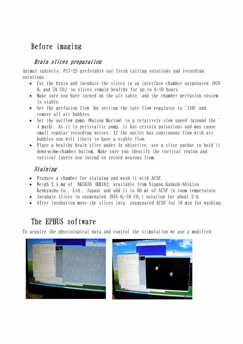
The EPHUS software

To acquire the physiological data and control the stimulation we use a modified

version of Ephus software (Ephus, available at https://openwiki.janelia.org/).

Turn on Q-imaging camera and open the Q-Capture software. Make sure your

electrophysiology amplifiers are turned on and configured. For the MultiCLamp this

includes running MultiClamp Commander and the MultiClamp Telegraph client.

The telegraph client (“Ephus” software interface) has to be scanned and connected

to

Multiclamp 700B, as shown above.

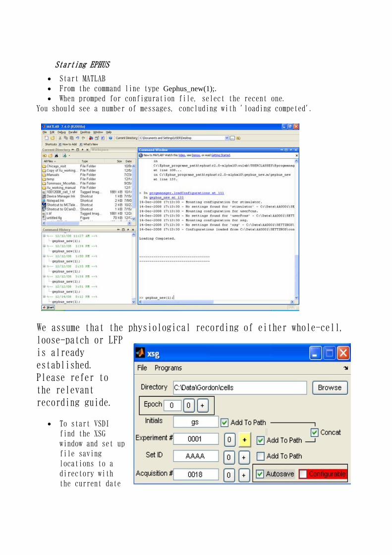
Starting EPHUS

Start MATLAB

From the command line type Gephus_new(1);. When promped for configuration file, select the recent one.

You should see a number of messages, concluding with 'loading competed'.

We assume that the physiological recording of either whole-cell,

loose-patch or LFP

is already

established.

Please refer to

the relevant

recording guide.

To start VSDI

find the XSG

window and set up

file saving

locations to a

directory with

the current date

in your own directory and put your initials.

The following part should be done only after the VSDI system is

ready for imaging (see below).

The image should be centered to the field of view of the VSDI camera.

Pull the lever marked 'VSDI' and snap a frame with the Q-imaging software

(see instructions) and save it to your experiment directory.

In the 'Hotswitch' window, press 'VSDI 8 s'. This should set all parameters

to recording VSDI to map stimulation at intevals of 8 seconds.

Running a mapping experiment

Specify the mapPattern and the spacing between positions.

Use “Grab video” to load the snap

picture via the Q-imaging software

(It is saved at the

corresponding cell folder).

You can label the cell soma by

clicking “[1]”

Use the '=' tick to set the X and Y

spacing to the same value. The

mapping grid should appear overlaid

on the videoImg window. Position

the map, both offset and rotation ,

using 'dX' 'dY' and 'deg'

You can click “Use as offset” to make

the pattern centering around the cell soma. For VSDI use 4x4 or 3x4 and cover the area of interest. Once the map is ready you can follow the instructions for BV and hit 'Map' when the

BV is ready.

The BV software

Setting the microscope for VSDI

Verify the filter position on the bottom to VSDI-filter (red arrow).

Remove the IR filter ･ pull low lever out.

Push lever on camera port in (marked VSDI)

Acquisition

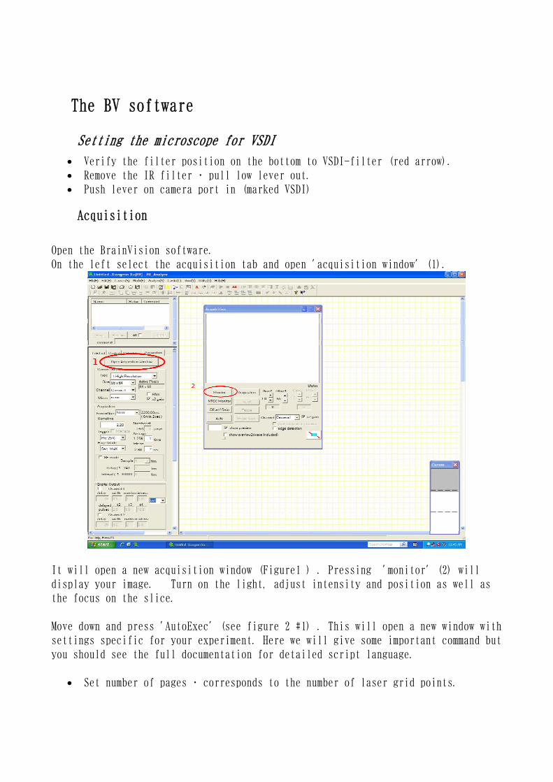
Open the BrainVision software.

On the left select the acquisition tab and open 'acquisition window' (1).

It will open a new acquisition window (Figure1 ) . Pressing 'monitor' (2) will

display your image. Turn on the light, adjust intensity and position as well as

the focus on the slice.

Move down and press 'AutoExec' (see figure 2 #1) . This will open a new window with

settings specific for your experiment. Here we will give some important command but

you should see the full documentation for detailed script language.

Set number of pages ･ corresponds to the number of laser grid points.

Create a directory in C:/Data with the current date.

Set 'save file'- to the current date

Note that for file naming you should put your initials followed by the date of the

experiment. After the date put “_” (underscore) and the cell number

corresponding to the XSG directory in the EPUS program.

Set 'save dir'- to the current date

Press 'test' button (3).

If the test is completed successfully you are ready to run the experiment.

You can now:

stop the monitor

stop perfusion

press start (4)

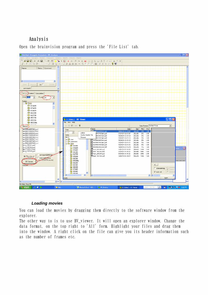
Analysis

Open the brainvision program and press the 'File List' tab.

Loading movies

You can load the movies by dragging them directly to the software window from the

explorer.

The other way to is to use BV_viewer. It will open an explorer window. Change the

data format, on the top right to 'All' form. Highlight your files and drag them

into the window. A right click on the file can give you its header information such

as the number of frames etc.

Double click on a frame and a rectangle will appear with a trace representing the

VSDI change in the region over time.

Press the calculation tab. While one frame is selected press 'Spatial Filter' (1)

and 'Cubic Filter' (2). For a quantitative measure it is necessary to select

reference frames. One way is to use the first 10 or 20 frames (3).

If you have multiple files loaded ･ as you normally would- after applying all these

changes to one file you should press 'Apply All' (4) to apply them to the rest of

the files.

Note that the reference frame is not applied and you will have to calculate is

separately for each file.

Press the 'Control' tab and scroll down.

At the trace, move the rectangle until a clear signal is seen. Then click on the

peak of the signal ･ a dashad line should mark your position on the trace.

When at the peak adjust 'Img' and 'Threshold' until a region is green or somewhat

redish (but not too much red). Make sure that when you click on the trace at the

pre-stimulus region it is mostly gray. If it is green or red redus 'Img' and

increase 'Threshold'.

To apply the settings to all files press 'Apply all' below 'step' then scroll down

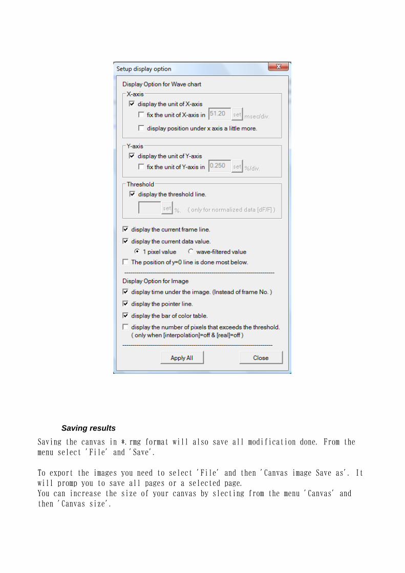
and apply all again below 'show option' .

It is usfull to set identical scale for all traces. To do so you need to press

'show Option'. In the window that opens up you can check 'fix the units of Y axis'

and select a value.

Saving results

Saving the canvas in *.rmg format will also save all modification done. From the

menu select 'File' and 'Save'.

To export the images you need to select 'File' and then 'Canvas image Save as'. It

will promp you to save all pages or a selected page.

You can increase the size of your canvas by slecting from the menu 'Canvas' and

then 'Canvas size'.

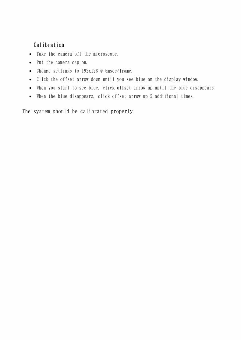
Calibration

Take the camera off the microscope.

Put the camera cap on.

Change settings to 192x128 @ 5msec/frame.

Click the offset arrow down until you see blue on the display window.

When you start to see blue, click offset arrow up until the blue disappears.

When the blue disappears, click offset arrow up 5 additional times.

The system should be calibrated properly.