Sample to Insight

Tutorial

Taxonomic Profiling of Whole Shotgun Metage-nomic Data

June 28, 2018

QIAGEN Aarhus Silkeborgvej 2 Prismet 8000 Aarhus C DenmarkTelephone: +45 70 22 32 44 www.qiagenbioinformatics.com ts-bioinformatics@qiagen.com

Tutorial

2

Taxonomic Profiling of Whole Shotgun Metagenomic DataThis tutorial will give an introduction to the use of the CLC Microbial Genomics Module TaxonomicProfiling tool on whole shotgun metagenomic data.

To demonstrate how to use the tools we will analyze a subset of the data from the publicationby Willmann et al., 2015. This paper describes two healthy male subjects (S1 and S2) whowere treated with the antibiotic ciprofloxacin (Cp) for 6 days. Stool samples were taken on day 0(before treatment), the first, third and sixth (last) day of treatment, and two and 28 days afterthe treatment. Metagenomic shotgun sequencing was performed on all samples on an IlluminaHiSeq 2000 platform using a paired-end sequencing approach with a targeted read length of 100bp and an insert size of 180 bp. In this tutorial, we will analyze the samples that were collectedbefore treatment (day 0), the last day of treatment (day 6) as well as 28 days after treatment(day 34). We will investigate how the composition of the gut microbiota develops over time inresponse to the treatment and in how far it recovers after the treatment.

Prerequisites For this tutorial, you will need either CLC Genomics Workbench or BiomedicalGenomics Workbench with CLC Microbial Genomics Module 3.5 or higher installed. How to in-stall modules and plugins is described here: http://resources.qiagenbioinformatics.com/manuals/clcmgm/current/index.php?manual=Installation_modules.html, aswell as in the module manual.

Overview In this tutorial we will go through the use of several different tools in order to monitorthe evolution of the gut microbiota of the two subjects before, during and after a ciprofloxacintreatment.

• First, we will import the NGS reads from the 6 samples to the workbench and prepare themfor analysis. We will also import reference databases of microbial genomes and metadata.

• Then we will run the Data QC and Taxonomic Profiling workflow to build a profile of thebacteria and their abundances in each sample.

• We will then run the Merge and Estimate Alpha and Beta Diversities workflow in order tomerge abundance profiles from each sample into a single table and measure diversity bothwithin and between samples.

• We then look at the tables, visualizations and plots that we have created and make someinteresting observations on the data.

• And finally, we create a heat map that shows how the samples cluster and how the differentorganism abundances correlate across the samples.

Tutorial

3

Downloading and importing the data The data for this tutorial consist of NGS data files fromthe Willmann et al., 2015 publication. The original files, the publication abstract and the fullmetadata are available directly from the workbench using the Search for Reads in SRA tool andlooking for the study accession number ERP011645.

However, to ensure a reasonable analysis time for this tutorial, we provide a dataset whereeach sample has been reduced to a million paired-end reads, a metadata spreadsheet, and acustomized reference database for identifying the composition of the gut microbiome.

1. Click on the following link or paste it into your web browser to download the tutorialdata: http://resources.qiagenbioinformatics.com/testdata/taxpro.zip.The zip-file being downloaded is ∼900MB, so depending on your internet connection, thismay take a while to download.

2. Start your workbench and create a folder for storing input data and results, named forexample Profiling tutorial.

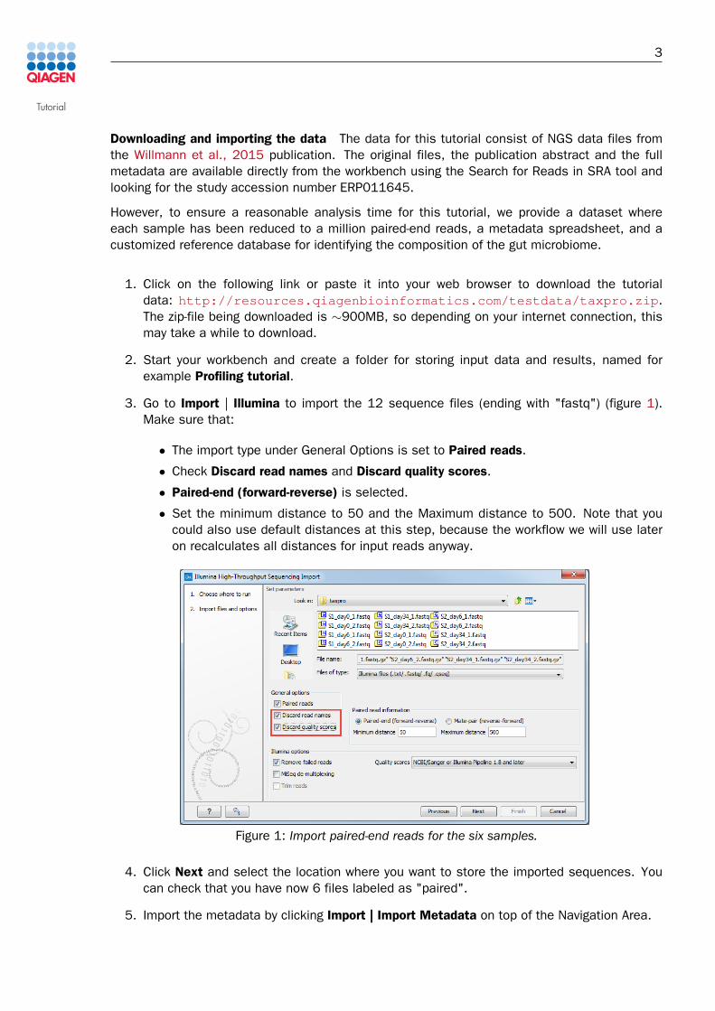
3. Go to Import | Illumina to import the 12 sequence files (ending with "fastq") (figure 1).Make sure that:

• The import type under General Options is set to Paired reads.

• Check Discard read names and Discard quality scores.

• Paired-end (forward-reverse) is selected.

• Set the minimum distance to 50 and the Maximum distance to 500. Note that youcould also use default distances at this step, because the workflow we will use lateron recalculates all distances for input reads anyway.

Figure 1: Import paired-end reads for the six samples.

4. Click Next and select the location where you want to store the imported sequences. Youcan check that you have now 6 files labeled as "paired".

5. Import the metadata by clicking Import | Import Metadata on top of the Navigation Area.

Tutorial

4

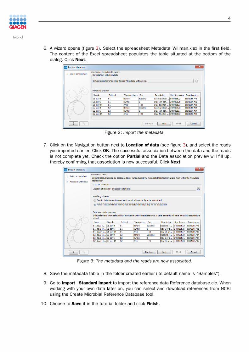
6. A wizard opens (figure 2). Select the spreadsheet Metadata_Willman.xlsx in the first field.The content of the Excel spreadsheet populates the table situated at the bottom of thedialog. Click Next.

Figure 2: Import the metadata.

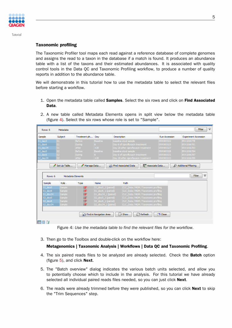
7. Click on the Navigation button next to Location of data (see figure 3), and select the readsyou imported earlier. Click OK. The successful association between the data and the readsis not complete yet. Check the option Partial and the Data association preview will fill up,thereby confirming that association is now successful. Click Next.

Figure 3: The metadata and the reads are now associated.

8. Save the metadata table in the folder created earlier (its default name is "Samples").

9. Go to Import | Standard import to import the reference data Reference database.clc. Whenworking with your own data later on, you can select and download references from NCBIusing the Create Microbial Reference Database tool.

10. Choose to Save it in the tutorial folder and click Finish.

Tutorial

5

Taxonomic profiling

The Taxonomic Profiler tool maps each read against a reference database of complete genomesand assigns the read to a taxon in the database if a match is found. It produces an abundancetable with a list of the taxons and their estimated abundances. It is associated with qualitycontrol tools in the Data QC and Taxonomic Profiling workflow, to produce a number of qualityreports in addition to the abundance table.

We will demonstrate in this tutorial how to use the metadata table to select the relevant filesbefore starting a workflow.

1. Open the metadata table called Samples. Select the six rows and click on Find AssociatedData.

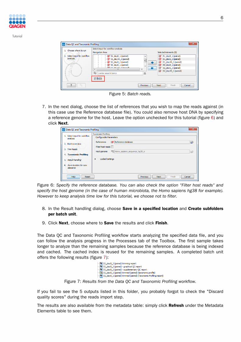
2. A new table called Metadata Elements opens in split view below the metadata table(figure 4). Select the six rows whose role is set to "Sample".

Figure 4: Use the metadata table to find the relevant files for the workflow.

3. Then go to the Toolbox and double-click on the workflow here:

Metagenomics | Taxonomic Analysis | Workflows | Data QC and Taxonomic Profiling.

4. The six paired reads files to be analyzed are already selected. Check the Batch option(figure 5), and click Next.

5. The "Batch overview" dialog indicates the various batch units selected, and allow youto potentially choose which to include in the analysis. For this tutorial we have alreadyselected all individual paired reads files needed, so you can just click Next.

6. The reads were already trimmed before they were published, so you can click Next to skipthe "Trim Sequences" step.

Tutorial

6

Figure 5: Batch reads.

7. In the next dialog, choose the list of references that you wish to map the reads against (inthis case use the Reference database file). You could also remove host DNA by specifyinga reference genome for the host. Leave the option unchecked for this tutorial (figure 6) andclick Next.

Figure 6: Specify the reference database. You can also check the option "Filter host reads" andspecify the host genome (in the case of human microbiota, the Homo sapiens hg38 for example).However to keep analysis time low for this tutorial, we choose not to filter.

8. In the Result handling dialog, choose Save in a specified location and Create subfoldersper batch unit.

9. Click Next, choose where to Save the results and click Finish.

The Data QC and Taxonomic Profiling workflow starts analyzing the specified data file, and youcan follow the analysis progress in the Processes tab of the Toolbox. The first sample takeslonger to analyze than the remaining samples because the reference database is being indexedand cached. The cached index is reused for the remaining samples. A completed batch unitoffers the following results (figure 7):

Figure 7: Results from the Data QC and Taxonomic Profiling workflow.

If you fail to see the 5 outputs listed in this folder, you probably forgot to check the "Discardquality scores" during the reads import step.

The results are also available from the metadata table: simply click Refresh under the MetadataElements table to see them.

Tutorial

7

Merge results and statistical analyses

While it is possible to review each set of batch results one after the other, it makes more senseto merge the abundance tables into one, and to perform statistical tests on the merged table,later using metadata layers for improved visualization. You can do that with the Merge andEstimate Alpha and Beta Diversities workflow.

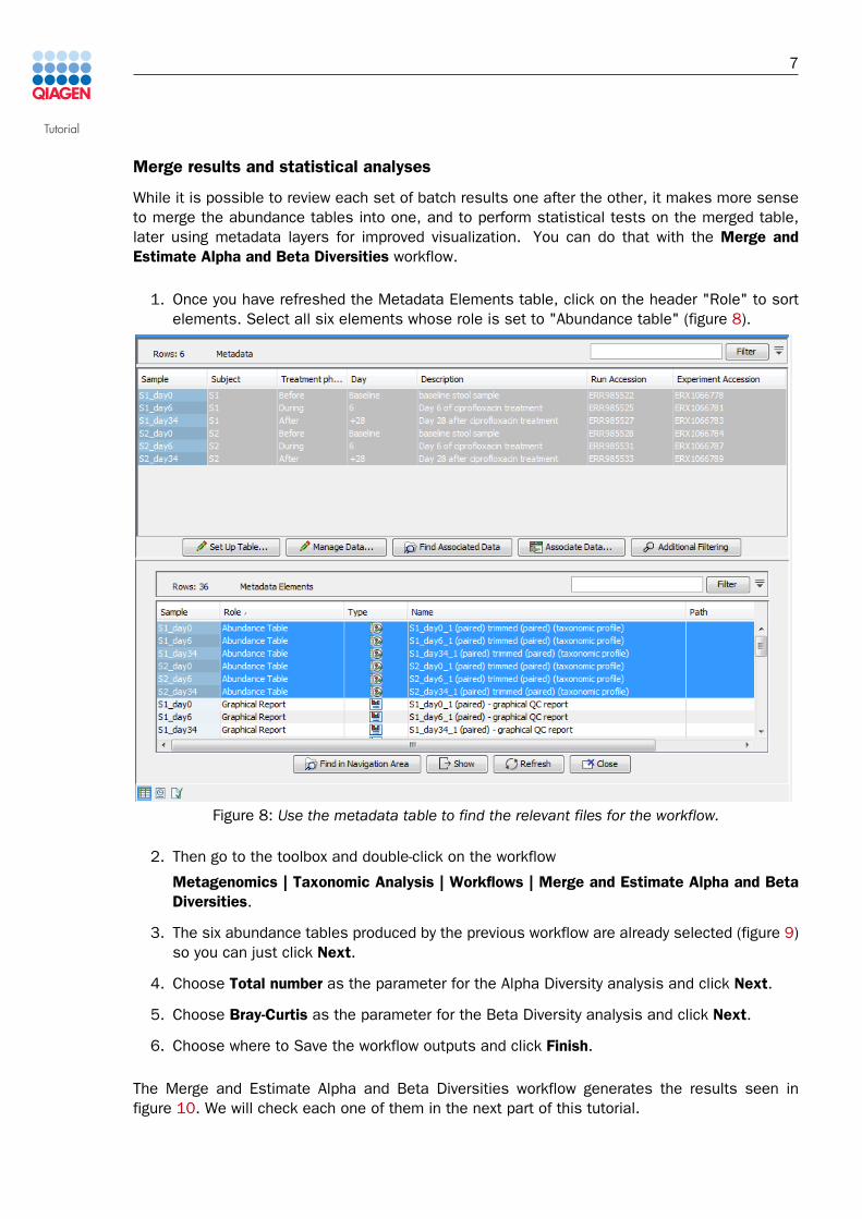
1. Once you have refreshed the Metadata Elements table, click on the header "Role" to sortelements. Select all six elements whose role is set to "Abundance table" (figure 8).

Figure 8: Use the metadata table to find the relevant files for the workflow.

2. Then go to the toolbox and double-click on the workflow

Metagenomics | Taxonomic Analysis | Workflows | Merge and Estimate Alpha and BetaDiversities.

3. The six abundance tables produced by the previous workflow are already selected (figure 9)so you can just click Next.

4. Choose Total number as the parameter for the Alpha Diversity analysis and click Next.

5. Choose Bray-Curtis as the parameter for the Beta Diversity analysis and click Next.

6. Choose where to Save the workflow outputs and click Finish.

The Merge and Estimate Alpha and Beta Diversities workflow generates the results seen infigure 10. We will check each one of them in the next part of this tutorial.

Tutorial

8

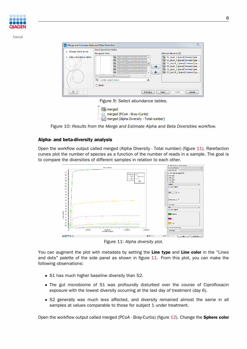
Figure 9: Select abundance tables.

Figure 10: Results from the Merge and Estimate Alpha and Beta Diversities workflow.

Alpha- and beta-diversity analysis

Open the workflow output called merged (Alpha Diversity - Total number) (figure 11). Rarefactioncurves plot the number of species as a function of the number of reads in a sample. The goal isto compare the diversities of different samples in relation to each other.

Figure 11: Alpha diversity plot.

You can augment the plot with metadata by setting the Line type and Line color in the "Linesand dots" palette of the side panel as shown in figure 11. From this plot, you can make thefollowing observations:

• S1 has much higher baseline diversity than S2.

• The gut microbiome of S1 was profoundly disturbed over the course of Ciprofloxacinexposure with the lowest diversity occurring at the last day of treatment (day 6).

• S2 generally was much less affected, and diversity remained almost the same in allsamples at values comparable to those for subject 1 under treatment.

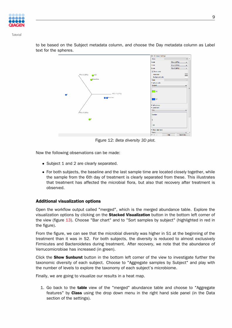
Open the workflow output called merged (PCoA - Bray-Curtis) (figure 12). Change the Sphere color

Tutorial

9

to be based on the Subject metadata column, and choose the Day metadata column as Labeltext for the spheres.

Figure 12: Beta diversity 3D plot.

Now the following observations can be made:

• Subject 1 and 2 are clearly separated.

• For both subjects, the baseline and the last sample time are located closely together, whilethe sample from the 6th day of treatment is clearly separated from these. This illustratesthat treatment has affected the microbial flora, but also that recovery after treatment isobserved.

Additional visualization options

Open the workflow output called "merged", which is the merged abundance table. Explore thevisualization options by clicking on the Stacked Visualization button in the bottom left corner ofthe view (figure 13). Choose "Bar chart" and to "Sort samples by subject" (highlighted in red inthe figure).

From the figure, we can see that the microbial diversity was higher in S1 at the beginning of thetreatment than it was in S2. For both subjects, the diversity is reduced to almost exclusivelyFirmicutes and Bacteroidetes during treatment. After recovery, we note that the abundance ofVerrucomicrobiae has increased (in green).

Click the Show Sunburst button in the bottom left corner of the view to investigate further thetaxonomic diversity of each subject. Choose to "Aggregate samples by Subject" and play withthe number of levels to explore the taxonomy of each subject’s microbiome.

Finally, we are going to visualize our results in a heat map.

1. Go back to the table view of the "merged" abundance table and choose to "Aggregatefeatures" by Class using the drop down menu in the right hand side panel (in the Datasection of the settings).

Tutorial

10

Figure 13: Relative abundances of microbial diversity over the course of treatment.

2. The resulting abundance table has 12 rows. Select them all and click Create AbundanceSubtable below the table.

3. A new table called Merged (Filtered) opens in split view (figure 14). Save it in the NavigationArea by dragging the tab to the location you want to save it.

Figure 14: Create an abundance table where features are aggregated by class.

4. In the Toolbox, go to

Metagenomics | Abundance Analysis | Create Heat Map for Abundance Table

5. Select the merged (Filtered) table you just created (figure 15).

Tutorial

11

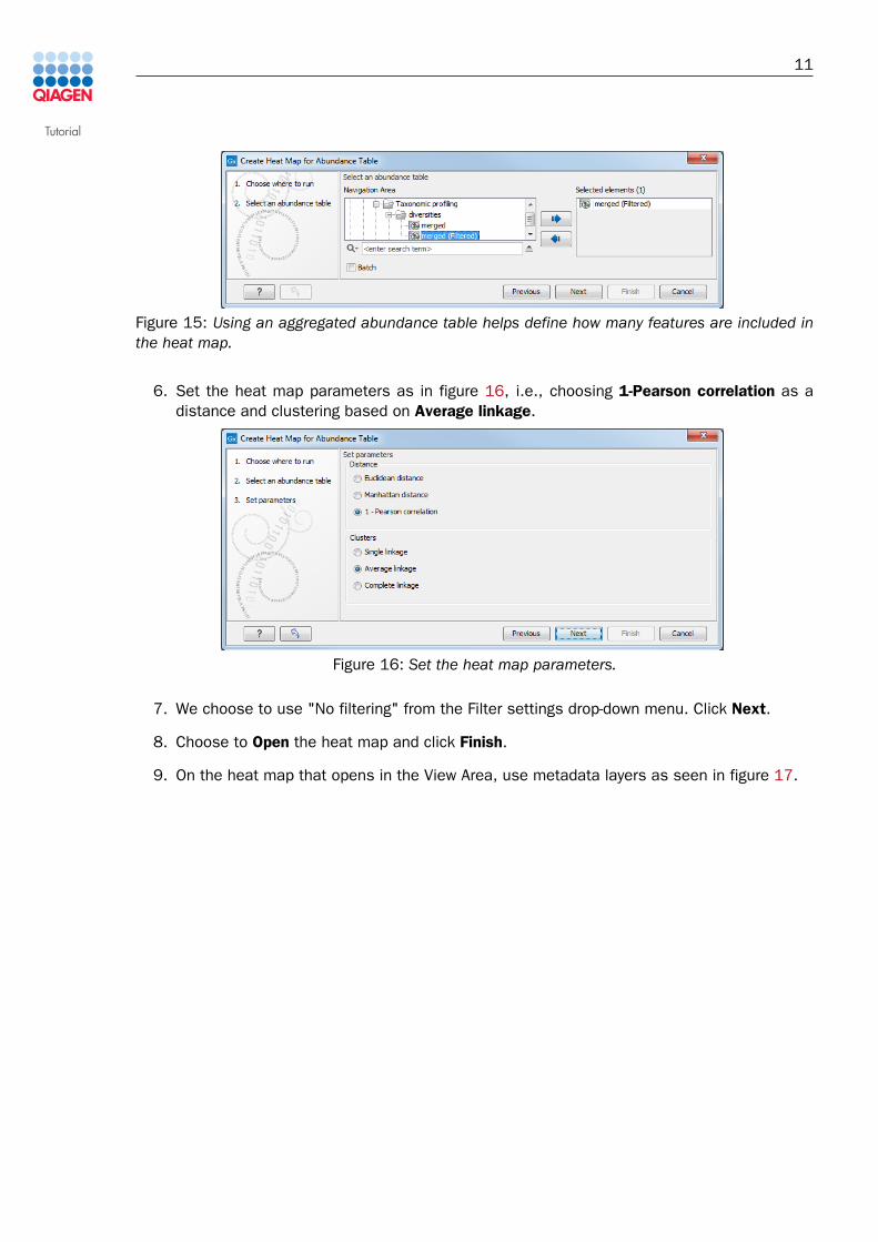
Figure 15: Using an aggregated abundance table helps define how many features are included inthe heat map.

6. Set the heat map parameters as in figure 16, i.e., choosing 1-Pearson correlation as adistance and clustering based on Average linkage.

Figure 16: Set the heat map parameters.

7. We choose to use "No filtering" from the Filter settings drop-down menu. Click Next.

8. Choose to Open the heat map and click Finish.

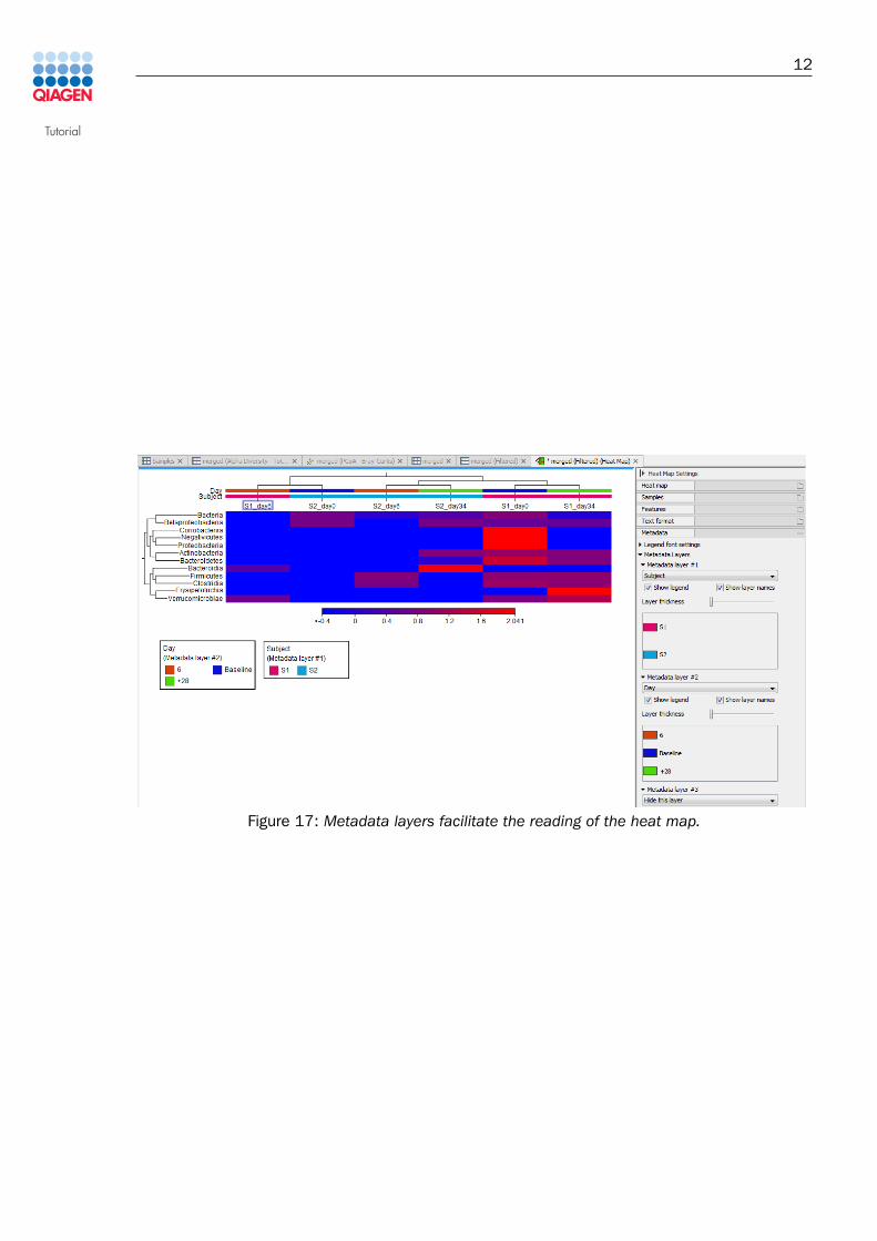
9. On the heat map that opens in the View Area, use metadata layers as seen in figure 17.

Tutorial

12

Figure 17: Metadata layers facilitate the reading of the heat map.

Tutorial

Bibliography

[Willmann et al., 2015] Willmann, M., El-Hadidi, M., Huson, D., Schuetz, M., Weidenmaier, C.,Autenrieth, I., and Peter, S. (2015). Antibiotic selection pressure determination throughsequence-based metagenomics. Antimicrobial Agents and Chemotherapy, 59(12):7335--7345.doi: 10.1128/AAC.01504-15.

13