Tutorial - QIAGEN · PDF fileThis tutorial takes you through some of the sequence analysis and structure visualization features ... CLC5, and CLC6 proteins. You can read more about

Sample to Insight

Tutorial

Exploring your proteinMarch 31, 2016

CLC bio, a QIAGEN Company Silkeborgvej 2 Prismet 8000 Aarhus C DenmarkTelephone: +45 70 22 32 44 www.clcbio.com [email protected]

Tutorial

Exploring your protein 2

Exploring your proteinThis tutorial takes you through some of the sequence analysis and structure visualization featuresavailable in CLC Drug Discovery Workbench.

Amino acid sequences and a protein structure of a chloride channel (CLC) protein are studied, tomake an initial exploration of whether inhibition of CLC proteins in E. coli could be used to combatE. coli infections in human. To judge if the chloride channel is sufficiently different between E. coliand human to vouch for a selective drug, human homologs are compared to E. coli CLC protein.A suitable protein structure of the CLC protein is found and examined with the intent to use it forstructure based drug design.

Example data relating to this tutorial can be imported from the Help menu ( Help | Import ExampleData). The files for this tutorial is found in CLC_Data/Example Data/Explore your Protein.

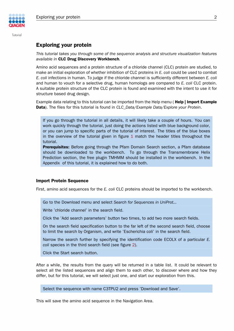
If you go through the tutorial in all details, it will likely take a couple of hours. You canwork quickly through the tutorial, just doing the actions listed with blue background color,or you can jump to specific parts of the tutorial of interest. The titles of the blue boxesin the overview of the tutorial given in figure 1 match the header titles throughout thetutorial.Prerequisites: Before going through the Pfam Domain Search section, a Pfam databaseshould be downloaded to the workbench. To go through the Transmembrane HelixPrediction section, the free plugin TMHMM should be installed in the workbench. In theAppendix of this tutorial, it is explained how to do both.

Import Protein Sequence

First, amino acid sequences for the E. coli CLC proteins should be imported to the workbench.

Go to the Download menu and select Search for Sequences in UniProt...

Write ’chloride channel’ in the search field.

Click the ’Add search parameters’ button two times, to add two more search fields.

On the search field specification button to the far left of the second search field, chooseto limit the search by Organism, and write ’Escherichia coli’ in the search field.

Narrow the search further by specifying the identification code ECOLX of a particular E.coli species in the third search field (see figure 2).

Click the Start search button.

After a while, the results from the query will be returned in a table list. It could be relevant toselect all the listed sequences and align them to each other, to discover where and how theydiffer, but for this tutorial, we will select just one, and start our exploration from this.

Select the sequence with name C3TPU2 and press ’Download and Save’.

This will save the amino acid sequence in the Navigation Area.

Tutorial


Figure 1: Schematic of the tutorial workflow. Example file names are shown in italic.

BLAST to find Human Homologs

To discover if there are proteins in humans that are so similar to the E. coli CLC protein, that theywould likely be targeted by the same drugs, do a BLAST search for human homologs.

Invoke the BLAST at NCBI... tool from the Sequence Analysis | BLAST folder in the Toolbox.

Step 1: Select the saved CLC amino acid sequence as input.

Step 2: Use the blastp program on the Swiss-Prot protein sequences database (figure 3).

Step 3: Limit the search to Homo sapiens [ORGN]. Leave the rest as default values.

Step 4: Choose to open the results and click Finish.

After a few minutes, the BLAST results appear, showing an overview of how the hits align to thequery sequence.

Tutorial


Figure 2: Searching for E. coli chloride channels (example file UniProt search).

Figure 3: Program and database used for the BLAST search.

Right-click on the BLAST result overview and click Show | BLAST Table

or use the table icon below the view, as seen in figure 4.

Figure 4: Alternative views on BLAST results. The BLAST table is number two from the left.

Info box: Columns in the BLAST Table

Use the mouse to decrease or increase the column widths in the BLAST Table. Hold themouse pointer over the line dividing columns in the header row. When a left-right arrowappears, click and hold while dragging the size of the column to the desired width.

Sort the table based on E-value by clicking the E-value column header.

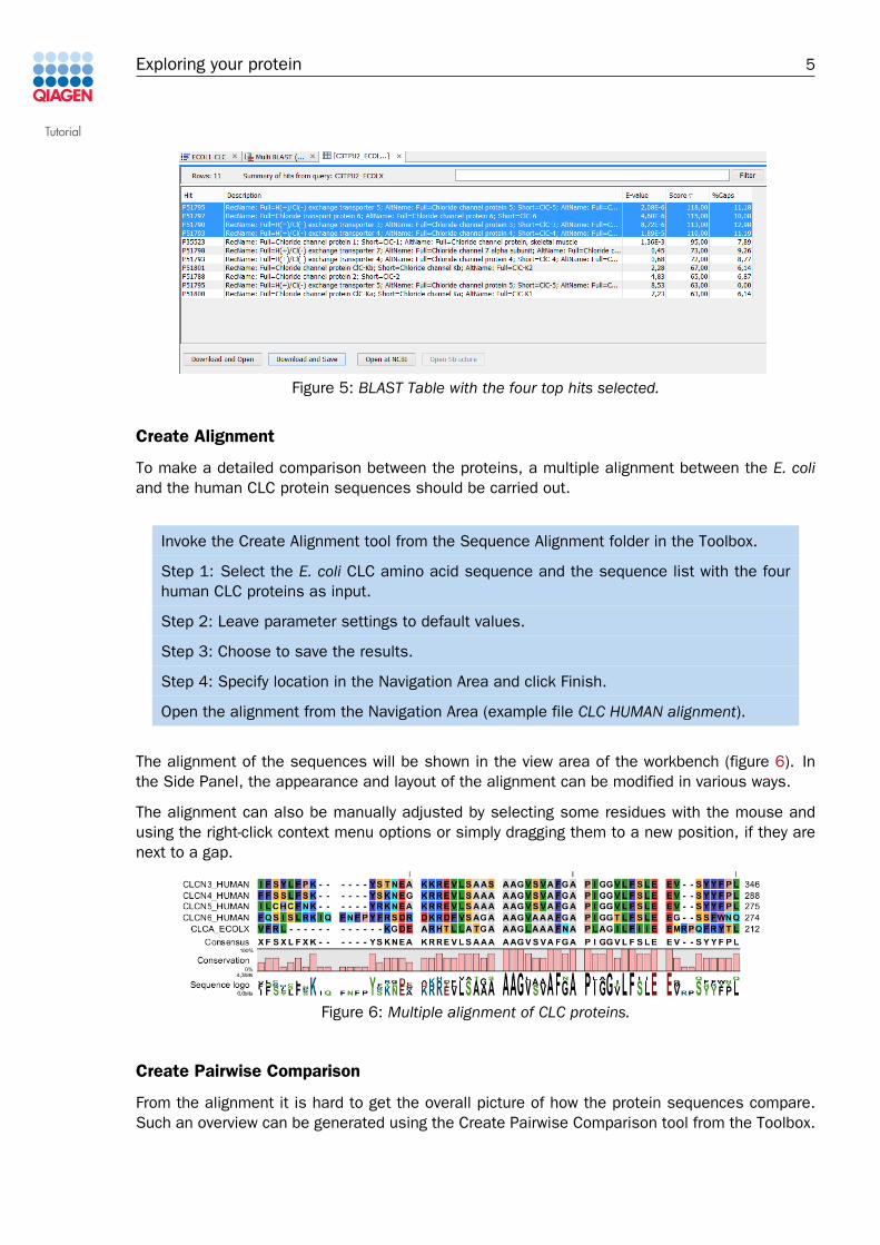
Select the four hits with highest score and lowest E-value (figure 5).

Click Download and Save.

The four top hits are the human CLC3, CLC4, CLC5, and CLC6 proteins. You can read more aboutBLAST and E-values in the Bioinformatics explained: BLAST section in the CLC Drug DiscoveryWorkbench manual.

Tutorial


Figure 5: BLAST Table with the four top hits selected.

Create Alignment

To make a detailed comparison between the proteins, a multiple alignment between the E. coliand the human CLC protein sequences should be carried out.

Invoke the Create Alignment tool from the Sequence Alignment folder in the Toolbox.

Step 1: Select the E. coli CLC amino acid sequence and the sequence list with the fourhuman CLC proteins as input.

Step 2: Leave parameter settings to default values.

Step 3: Choose to save the results.

Step 4: Specify location in the Navigation Area and click Finish.

Open the alignment from the Navigation Area (example file CLC HUMAN alignment).

The alignment of the sequences will be shown in the view area of the workbench (figure 6). Inthe Side Panel, the appearance and layout of the alignment can be modified in various ways.

The alignment can also be manually adjusted by selecting some residues with the mouse andusing the right-click context menu options or simply dragging them to a new position, if they arenext to a gap.

Figure 6: Multiple alignment of CLC proteins.

Create Pairwise Comparison

From the alignment it is hard to get the overall picture of how the protein sequences compare.Such an overview can be generated using the Create Pairwise Comparison tool from the Toolbox.

Tutorial


Invoke the Create Pairwise Comparison tool from the Sequence Alignment folder in theToolbox.

Step 1: Select the alignment as input.

Step 2: Leave default values.

Step 3: Choose to open results and click Finish.

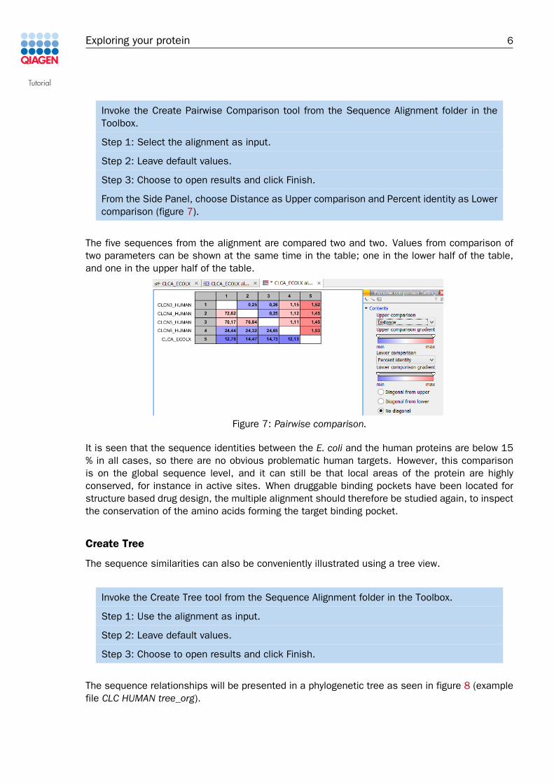
From the Side Panel, choose Distance as Upper comparison and Percent identity as Lowercomparison (figure 7).

The five sequences from the alignment are compared two and two. Values from comparison oftwo parameters can be shown at the same time in the table; one in the lower half of the table,and one in the upper half of the table.

Figure 7: Pairwise comparison.

It is seen that the sequence identities between the E. coli and the human proteins are below 15% in all cases, so there are no obvious problematic human targets. However, this comparisonis on the global sequence level, and it can still be that local areas of the protein are highlyconserved, for instance in active sites. When druggable binding pockets have been located forstructure based drug design, the multiple alignment should therefore be studied again, to inspectthe conservation of the amino acids forming the target binding pocket.

Create Tree

The sequence similarities can also be conveniently illustrated using a tree view.

Invoke the Create Tree tool from the Sequence Alignment folder in the Toolbox.

Step 1: Use the alignment as input.

Step 2: Leave default values.

Step 3: Choose to open results and click Finish.

The sequence relationships will be presented in a phylogenetic tree as seen in figure 8 (examplefile CLC HUMAN tree_org).

Tutorial


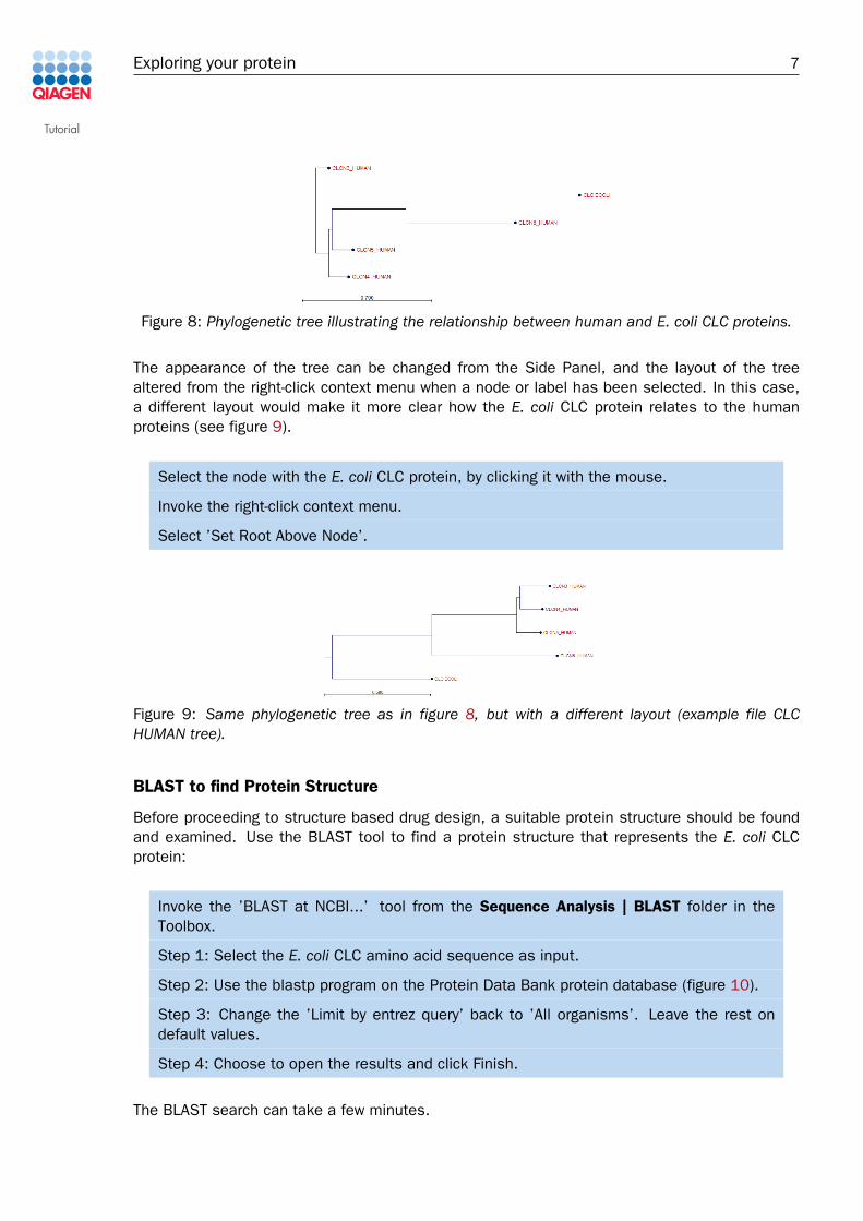
Figure 8: Phylogenetic tree illustrating the relationship between human and E. coli CLC proteins.

The appearance of the tree can be changed from the Side Panel, and the layout of the treealtered from the right-click context menu when a node or label has been selected. In this case,a different layout would make it more clear how the E. coli CLC protein relates to the humanproteins (see figure 9).

Select the node with the E. coli CLC protein, by clicking it with the mouse.

Invoke the right-click context menu.

Select ’Set Root Above Node’.

Figure 9: Same phylogenetic tree as in figure 8, but with a different layout (example file CLCHUMAN tree).

BLAST to find Protein Structure

Before proceeding to structure based drug design, a suitable protein structure should be foundand examined. Use the BLAST tool to find a protein structure that represents the E. coli CLCprotein:

Invoke the ’BLAST at NCBI...’ tool from the Sequence Analysis | BLAST folder in theToolbox.

Step 1: Select the E. coli CLC amino acid sequence as input.

Step 2: Use the blastp program on the Protein Data Bank protein database (figure 10).

Step 3: Change the ’Limit by entrez query’ back to ’All organisms’. Leave the rest ondefault values.

Step 4: Choose to open the results and click Finish.

The BLAST search can take a few minutes.

Tutorial


Figure 10: Program and database used for the BLAST search.

Right-click on the BLAST result overview and select Show | BLAST Table

There are several hits that match the query sequence completely, with very high scores and anE-value of zero.

Select the protein with the hit ID 1KPK_A in the table.

Click Open Structure.

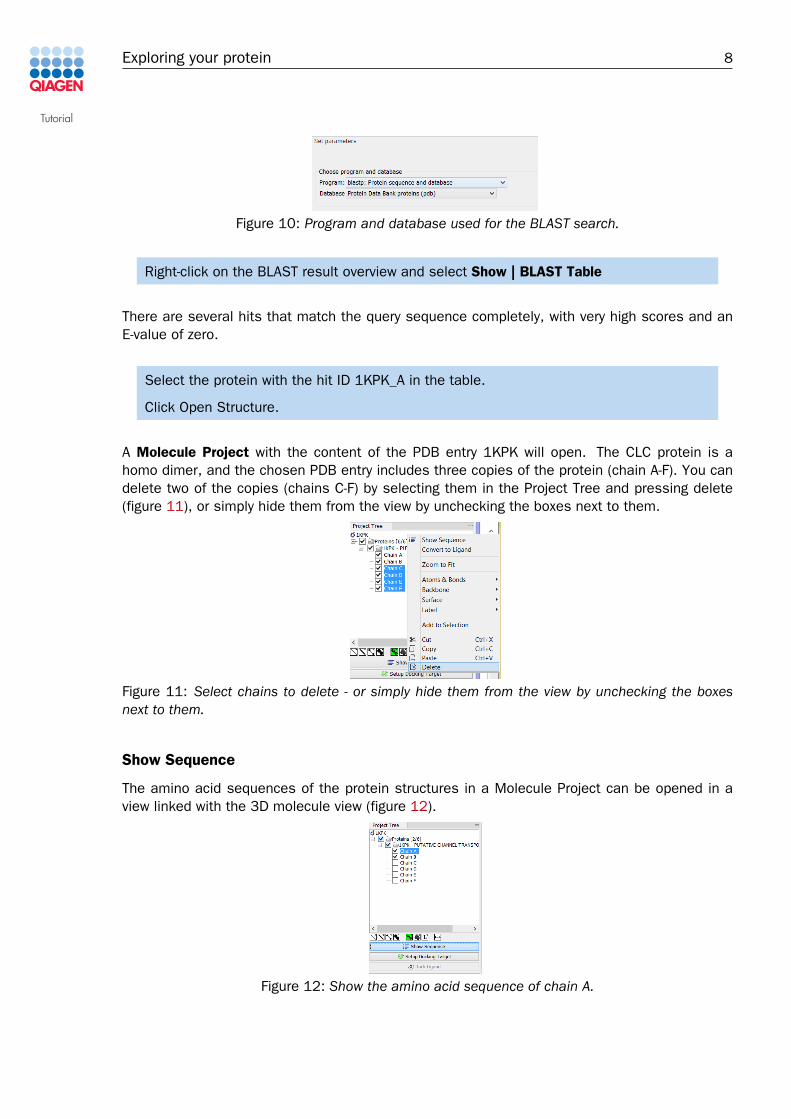
A Molecule Project with the content of the PDB entry 1KPK will open. The CLC protein is ahomo dimer, and the chosen PDB entry includes three copies of the protein (chain A-F). You candelete two of the copies (chains C-F) by selecting them in the Project Tree and pressing delete(figure 11), or simply hide them from the view by unchecking the boxes next to them.

Figure 11: Select chains to delete - or simply hide them from the view by unchecking the boxesnext to them.

Show Sequence

The amino acid sequences of the protein structures in a Molecule Project can be opened in aview linked with the 3D molecule view (figure 12).

Figure 12: Show the amino acid sequence of chain A.

Tutorial


Select Chain A in the Project Tree.

Click the Show Sequence button below the Project Tree.

A sequence list with the amino acid sequence of chain A will appear in split view.

Try to select a stretch of amino acids by click-drag the mouse over the sequence. This will zoomto the selected residues in the 3D view, and make a Current selection available in the ProjectTree. The atom selection only includes the backbone atoms, but all atoms of the amino acids areshown, to display the ’context’ of the selected backbone atoms. Click the Current selection in theProject Tree. This will put a blue box around the entry, to illustrate that it has been selected in theProject Tree view. The right-click context menu now allows you to create an atom group from theatom selection (backbone atoms) or from the selection plus context (all atoms in the residuesselected in the sequence view). The created atom groups can be treated as the molecules in theProject Tree (hide/show, modify visual representation and rename).

Info box: Link between sequence and structure

The link between the sequence in the Sequence List and the structure in the MoleculeProject will break if one of them is closed. Sequences opened from a Molecule Projectcan be used as input to the tools found in the Sequence Analysis folder in the Toolbox.Many of the tools will add annotation to the sequence. If the link between sequence andstructure is maintained, the sequence annotations can conveniently be visualized in theprotein structure context, by simply selecting the annotation in the sequence view andmaking a custom visualization of the generated Current atom selection in the 3D view.

Pfam Domain Search

Proteins are generally composed of one or more functional regions, commonly termed domains.The identification of domains that occur within proteins can therefore provide insights intotheir function. The Pfam database is a large collection of protein families, each representedby a model based on multiple sequence alignments. You can read more about Pfam athttp://pfam.sanger.ac.uk/.

Sequences in the workbench can be annotated with functional domains using the Pfam DomainSearch tool.

Make sure the protein sequence view is in focus (has a blue line in the top of the view).

Invoke the Pfam Domain Search tool from the Sequence Analysis folder in the Toolbox.

Step 1: The Sequence List with the protein sequence has already be selected as input.

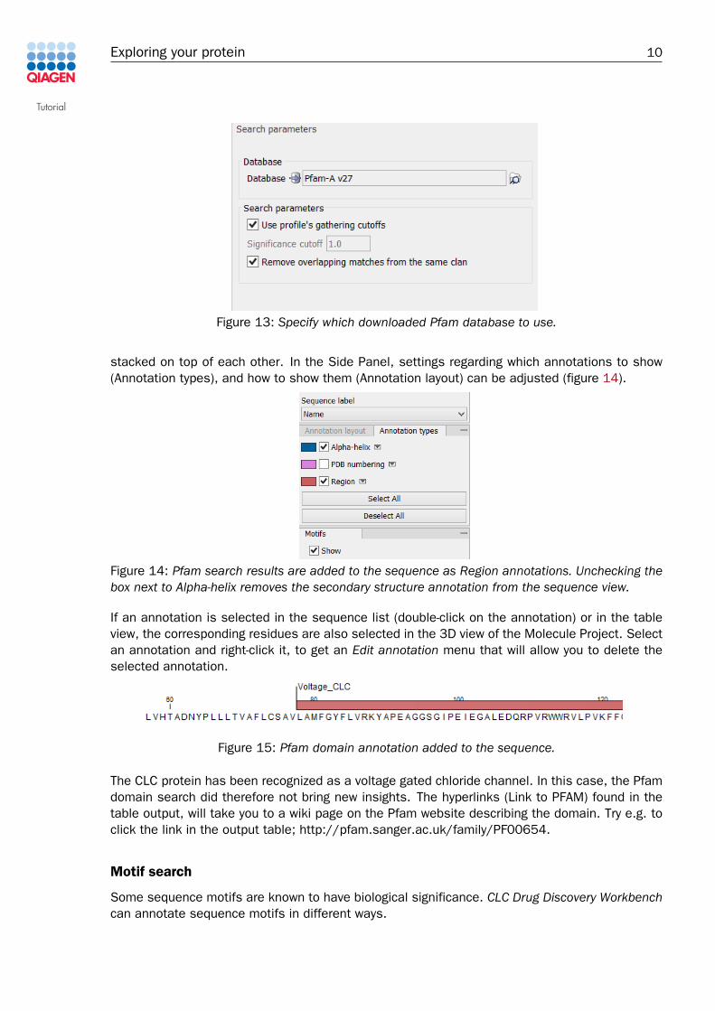
Step 2: Specify which Pfam database you wish to use (figure 13). If no Pfam databasehas yet been downloaded to your Navigation Area, see in the Appendix of this tutorialhow to do this.

Step 3: Choose to add annotation to sequence, create a table, open the results and clickFinish.

When the search is done, Pfam annotation is added to the sequence (figure 15). Secondarystructure annotation was already present, and it can be too crowded to look at many annotations

Tutorial


Figure 13: Specify which downloaded Pfam database to use.

stacked on top of each other. In the Side Panel, settings regarding which annotations to show(Annotation types), and how to show them (Annotation layout) can be adjusted (figure 14).

Figure 14: Pfam search results are added to the sequence as Region annotations. Unchecking thebox next to Alpha-helix removes the secondary structure annotation from the sequence view.

If an annotation is selected in the sequence list (double-click on the annotation) or in the tableview, the corresponding residues are also selected in the 3D view of the Molecule Project. Selectan annotation and right-click it, to get an Edit annotation menu that will allow you to delete theselected annotation.

Figure 15: Pfam domain annotation added to the sequence.

The CLC protein has been recognized as a voltage gated chloride channel. In this case, the Pfamdomain search did therefore not bring new insights. The hyperlinks (Link to PFAM) found in thetable output, will take you to a wiki page on the Pfam website describing the domain. Try e.g. toclick the link in the output table; http://pfam.sanger.ac.uk/family/PF00654.

Motif search

Some sequence motifs are known to have biological significance. CLC Drug Discovery Workbenchcan annotate sequence motifs in different ways.

Tutorial


As the CLC protein is positioned in a membrane, it could be relevant to know if it has binding sitesfor cholesterol, which is known to have a regulatory effect for some membrane proteins [Fantiniand Barrantes, 2013]. The best known cholesterol binding motif is the CRAC motif [Fantini andBarrantes, 2013], and the inverted domain, CARC. Such a motif can be searched for using theMotif Search tool from the toolbox.


Invoke the Motif Search tool from the Sequence Analysis folder in the Toolbox.


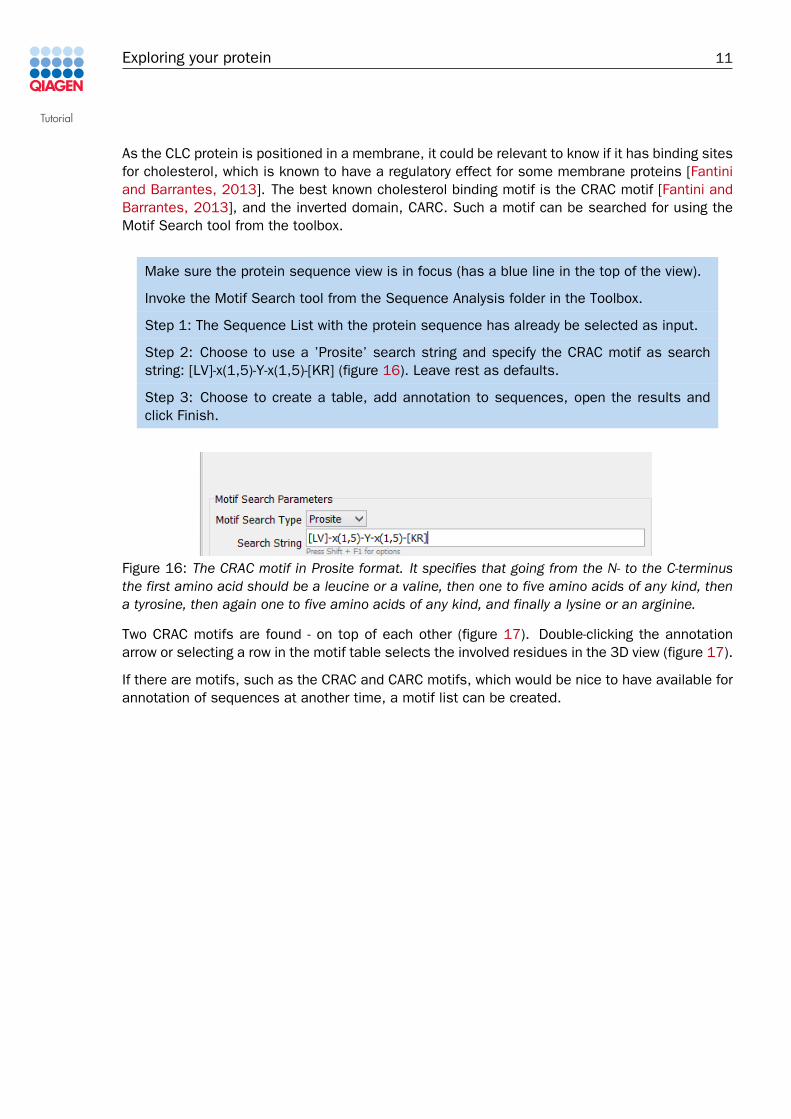
Step 2: Choose to use a ’Prosite’ search string and specify the CRAC motif as searchstring: [LV]-x(1,5)-Y-x(1,5)-[KR] (figure 16). Leave rest as defaults.

Step 3: Choose to create a table, add annotation to sequences, open the results andclick Finish.

Figure 16: The CRAC motif in Prosite format. It specifies that going from the N- to the C-terminusthe first amino acid should be a leucine or a valine, then one to five amino acids of any kind, thena tyrosine, then again one to five amino acids of any kind, and finally a lysine or an arginine.

Two CRAC motifs are found - on top of each other (figure 17). Double-clicking the annotationarrow or selecting a row in the motif table selects the involved residues in the 3D view (figure 17).

If there are motifs, such as the CRAC and CARC motifs, which would be nice to have available forannotation of sequences at another time, a motif list can be created.

Tutorial


Figure 17: The CRAC motif is found, in a position likely to fit with a cholesterol positioned in one ofthe membrane leaflets.

Tutorial


Invoke the Create Motif List tool from the Sequence Analysis folder in the Toolbox.

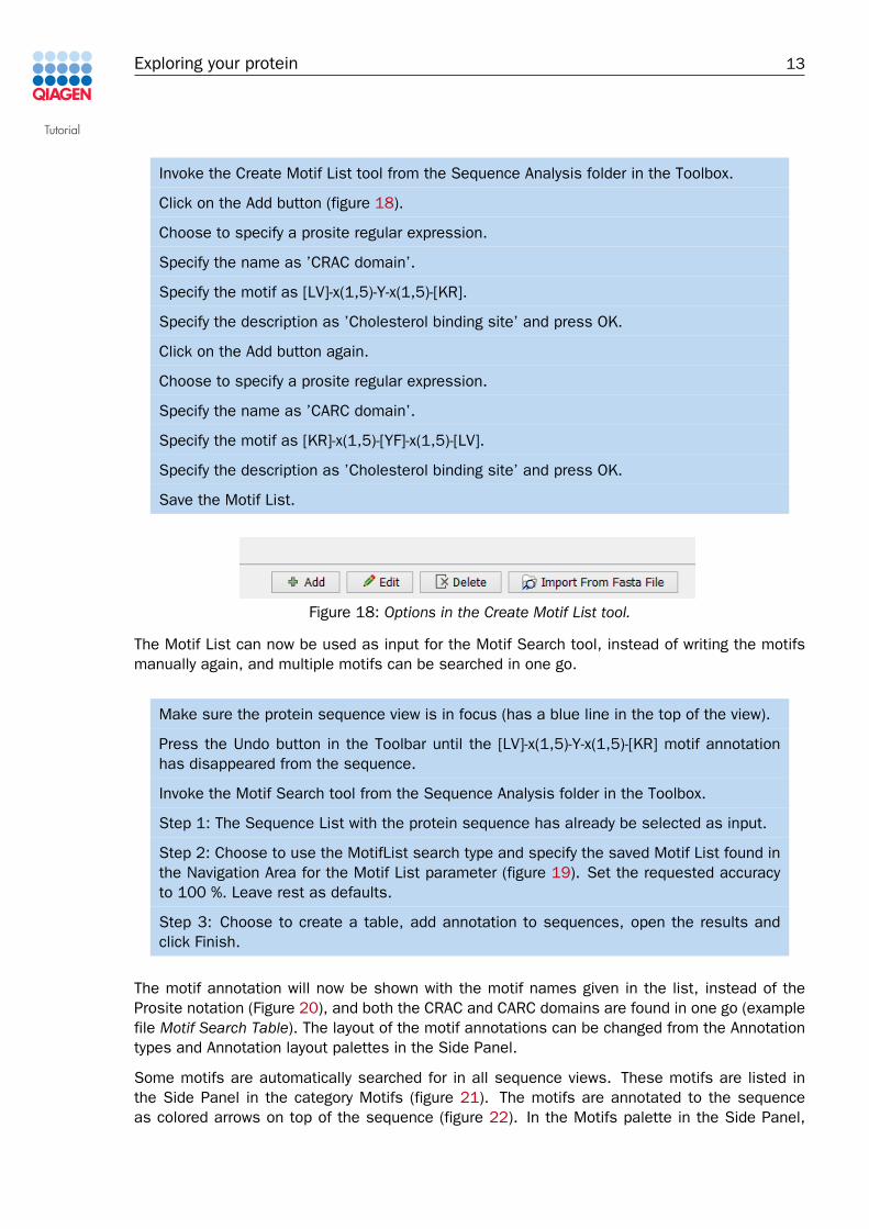
Click on the Add button (figure 18).

Choose to specify a prosite regular expression.

Specify the name as ’CRAC domain’.

Specify the motif as [LV]-x(1,5)-Y-x(1,5)-[KR].

Specify the description as ’Cholesterol binding site’ and press OK.

Click on the Add button again.

Choose to specify a prosite regular expression.

Specify the name as ’CARC domain’.

Specify the motif as [KR]-x(1,5)-[YF]-x(1,5)-[LV].

Specify the description as ’Cholesterol binding site’ and press OK.

Save the Motif List.

Figure 18: Options in the Create Motif List tool.

The Motif List can now be used as input for the Motif Search tool, instead of writing the motifsmanually again, and multiple motifs can be searched in one go.


Press the Undo button in the Toolbar until the [LV]-x(1,5)-Y-x(1,5)-[KR] motif annotationhas disappeared from the sequence.

Invoke the Motif Search tool from the Sequence Analysis folder in the Toolbox.


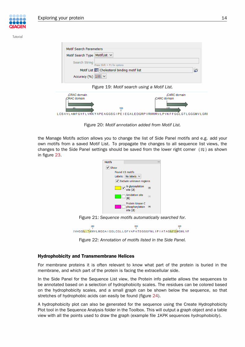
Step 2: Choose to use the MotifList search type and specify the saved Motif List found inthe Navigation Area for the Motif List parameter (figure 19). Set the requested accuracyto 100 %. Leave rest as defaults.

Step 3: Choose to create a table, add annotation to sequences, open the results andclick Finish.

The motif annotation will now be shown with the motif names given in the list, instead of theProsite notation (Figure 20), and both the CRAC and CARC domains are found in one go (examplefile Motif Search Table). The layout of the motif annotations can be changed from the Annotationtypes and Annotation layout palettes in the Side Panel.

Some motifs are automatically searched for in all sequence views. These motifs are listed inthe Side Panel in the category Motifs (figure 21). The motifs are annotated to the sequenceas colored arrows on top of the sequence (figure 22). In the Motifs palette in the Side Panel,

Tutorial


Figure 19: Motif search using a Motif List.

Figure 20: Motif annotation added from Motif List.

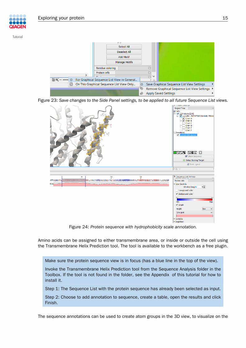
the Manage Motifs action allows you to change the list of Side Panel motifs and e.g. add yourown motifs from a saved Motif List. To propagate the changes to all sequence list views, thechanges to the Side Panel settings should be saved from the lower right corner ( ) as shownin figure 23.

Figure 21: Sequence motifs automatically searched for.

Figure 22: Annotation of motifs listed in the Side Panel.

Hydrophobicity and Transmembrane Helices

For membrane proteins it is often relevant to know what part of the protein is buried in themembrane, and which part of the protein is facing the extracellular side.

In the Side Panel for the Sequence List view, the Protein info palette allows the sequences tobe annotated based on a selection of hydrophobicity scales. The residues can be colored basedon the hydrophobicity scales, and a small graph can be shown below the sequence, so thatstretches of hydrophobic acids can easily be found (figure 24).

A hydrophobicity plot can also be generated for the sequence using the Create HydrophobicityPlot tool in the Sequence Analysis folder in the Toolbox. This will output a graph object and a tableview with all the points used to draw the graph (example file 1KPK sequences hydrophobicity).

Tutorial


Figure 23: Save changes to the Side Panel settings, to be applied to all future Sequence List views.

Figure 24: Protein sequence with hydrophobicity scale annotation.

Amino acids can be assigned to either transmembrane area, or inside or outside the cell usingthe Transmembrane Helix Prediction tool. The tool is available to the workbench as a free plugin.


Invoke the Transmembrane Helix Prediction tool from the Sequence Analysis folder in theToolbox. If the tool is not found in the folder, see the Appendix of this tutorial for how toinstall it.

Step 1: The Sequence List with the protein sequence has already been selected as input.

Step 2: Choose to add annotation to sequence, create a table, open the results and clickFinish.

The sequence annotations can be used to create atom groups in the 3D view, to visualize on the

Tutorial


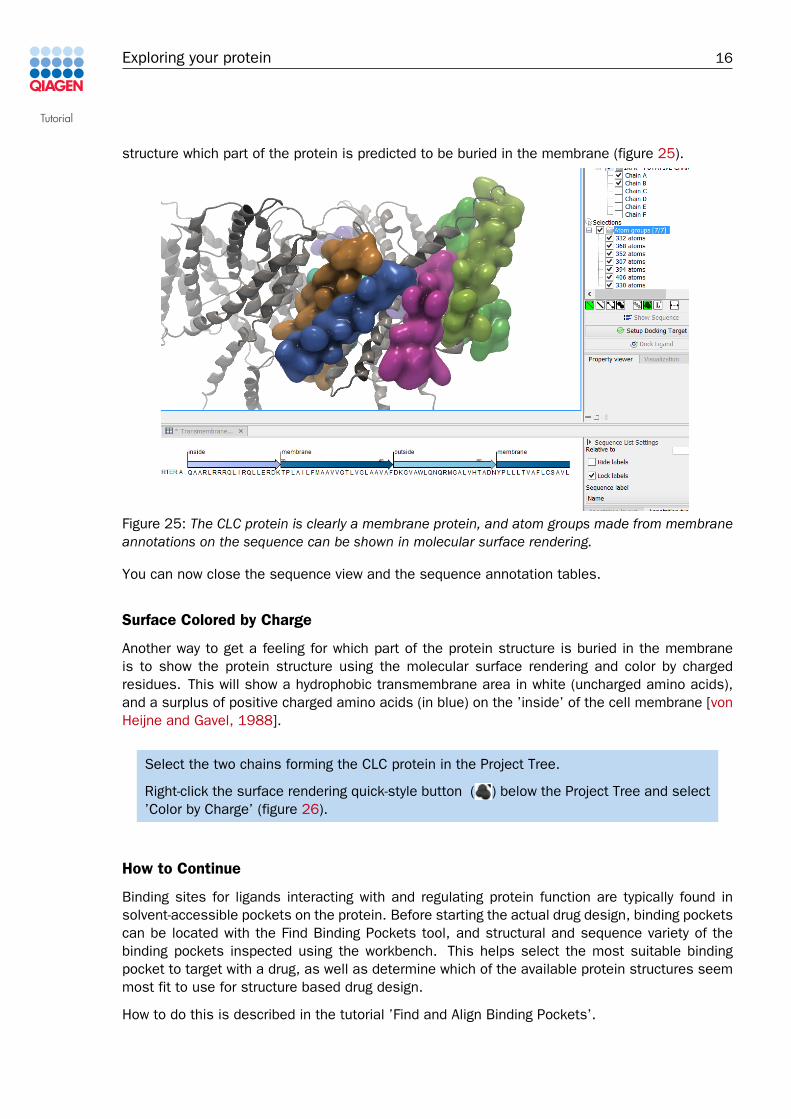
structure which part of the protein is predicted to be buried in the membrane (figure 25).

Figure 25: The CLC protein is clearly a membrane protein, and atom groups made from membraneannotations on the sequence can be shown in molecular surface rendering.

You can now close the sequence view and the sequence annotation tables.

Surface Colored by Charge

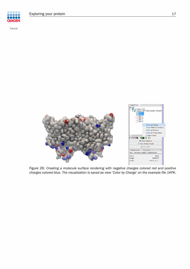
Another way to get a feeling for which part of the protein structure is buried in the membraneis to show the protein structure using the molecular surface rendering and color by chargedresidues. This will show a hydrophobic transmembrane area in white (uncharged amino acids),and a surplus of positive charged amino acids (in blue) on the ’inside’ of the cell membrane [vonHeijne and Gavel, 1988].

Select the two chains forming the CLC protein in the Project Tree.

Right-click the surface rendering quick-style button ( ) below the Project Tree and select’Color by Charge’ (figure 26).

How to Continue

Binding sites for ligands interacting with and regulating protein function are typically found insolvent-accessible pockets on the protein. Before starting the actual drug design, binding pocketscan be located with the Find Binding Pockets tool, and structural and sequence variety of thebinding pockets inspected using the workbench. This helps select the most suitable bindingpocket to target with a drug, as well as determine which of the available protein structures seemmost fit to use for structure based drug design.

How to do this is described in the tutorial ’Find and Align Binding Pockets’.

Tutorial


Figure 26: Creating a molecule surface rendering with negative charges colored red and positivecharges colored blue. The visualization is saved as view ’Color by Charge’ on the example file 1KPK.

Tutorial


Appendix

How to download the Pfam database

To download the Pfam database to the workbench, invoke the ’Download Pfam Database’ toolfrom the Sequence Analysis folder in the Toolbox. The will open a wizard where the only optionis to save the database. Click Next, and specify where in the Navigation Area you would like tosave the database. When you later run the ’Pfam Domain Search’ tool, this is the database tospecify in Step 2 (see figure 13).

How to install the TMHMM plugin for transmembrane helix prediction

If you do not see the Transmembrane Helix Prediction tool in the Sequence Analysis folder in theToolbox, you should download and install the TMHMM plugin to the workbench.

Invoke the plugins manager from the Toolbar (figure 27).

Figure 27: Click Plugins in the right side of the Toolbar to invoke the plugins manager.

Info box: Permissions in the plugins manager

Depending on your computer setup, it is required that you have administrator privilegesto manage plugins. In that case, it will be written in red in the bottom of the manager,and you will not be allowed to download and install anything. You should then closethe workbench and start it up again as administrator (on Windows you can right-click theworkbench launch icon on your desktop and select ’Run as administrator’).

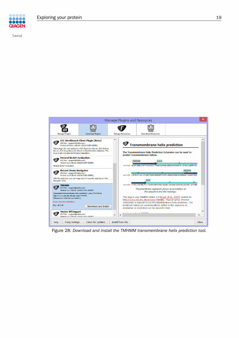
Click the Download Plugins tab in the plugins manager, select TMHMM from the list, and clickDownload and Install (figure 28).

Tutorial


Figure 28: Download and install the TMHMM transmembrane helix prediction tool.

Tutorial


References[Fantini and Barrantes, 2013] Fantini, J. and Barrantes, F. J. (2013). How cholesterol interacts

with membrane proteins: an exploration of cholesterol-binding sites including crac, carc andtilted domains. Frontiers in Physiology, 4(31).

[von Heijne and Gavel, 1988] von Heijne, G. and Gavel, Y. (1988). Topogenic signals in integralmembrane proteins. European Journal of Biochemistry, 174(4):671--678.

Documents

Tutorial - QIAGEN · PDF fileThis tutorial takes you through some of the sequence analysis and structure visualization features ... CLC5, and CLC6 proteins. You can read more about