Embed Size (px)
Citation preview
Two New Classes of Nonlinear Transformations for Accelerating the Convergence of Infinite Integrals and Series
David Levin
!School of Mathemutical Sciences Tel Aviv University Ramat Aviv, Israel
and
Avram Sidi
Computer Science Department Technion -Israel Institute of Technology Haifa, Israel
Transmitted by M. Scott
ABSTRACT
Two new classes of nonlinear transformations, the Dtransformation to accelerate the convergence of infinite integrals and the d-transformation to accelerate the convergence of infinite series, are presented. In the course of the development of these transformations two interesting asymptotic expansions, one for infinite integrals and the other for infinite series, are derived. The transformations D and d can easily be applied to infinite integrals /$’ f(t) dt whose integrands f( t ) satisfy linear differential equations of the form f(t)=Zr=:=, pk. t)f@)( t) and to infinite series X$&r) whose terms f(r) satisfy a linear difference equation of the form f(r) =X$&r pk( r) A’f(r), such that in both cases the pk have asymptotic expansions in inverse powers of their arguments. In order to be able to apply these transformations successfully one need not know explicitly the differential equation that the integrand satisfies or the difference equation that the terms of the series satisfy; mere knowledge of the existence of such a differential or difference equation and its order m is enough. This broadens the areas to which these methods can be applied. The connection between the 0 and d-transformations with some known transformations in shown. The use and the remarkable efficiency of the D and d-transformations are demonstrated through several numerical examples. The computational aspects of these transformations are described in detail.
APPLIED MATHEMATICS AND COMPUTATION 9: 175-215 (1981) 175
0 Elsevier North Holland, Inc., 1981
52 Vanderbilt Ave., New York, NY 10017 MQ&vm9 ,Q, ,n_lnl7+lrl~no v=
176 DAVID LJWIN AND AVFL4M SIDI
1. INTRODUCTION
In this work we present some nonlinear transformations to accelerate the convergence of slowly converging infinite integrals and infinite series. These transformations, in a sense, combine the Gtransformation of Gray, Atchison, and McWilliams [l] and the confluent e-algorithm of Wynn [4] on the one hand, and some transformations that were obtained by the first author [S-7] for accelerating the convergence of infinite integrals and series on the other.
The Gtransformation and the confluent e-algorithm have in common the property that they integrate exactly from zero to infinity functions f(t) which satisfy linear differential equations with constant coefficients on (0, co); i.e., (in the notation of Gray, Atchison, and McWilliams [l]) the quantity G,[ F(t); k] of the Gtransformation and (in the notation of Wynn [4]) the quantity e&t) of the confluent r-algorithm are exactly equal to 17 f(t) dt. For more details on both the Gtransformation and the confluent r-algorithm the reader is referred to [l].
For future reference, when dealing with infinite series, we define Acy) to be the set of functions a(x), which, as x + co, have asymptotic expansions in inverse powers of x, of the form
(14
and when dealing with infinite integrals, we define Acy) to be the set of infinitely differentiable functions a(x), satisfying (l.l), and such that their derivatives of any order have asymptotic expansions, which can be obtained by differentiating that in (1.1) formally term by term,
It turns out numerically. that the G-transformation and the confluent e-algorithm work efficiently on functions of the form f = ug, where a E A(7) for some y and where g satisfies a linear differential equation with constant coefficients, provided F(x)= &f(t) dt is not monotonic as x + co-and therefore, on sums of functions of this form.
In the work of Levin [S] too we find that there is a strong connection between the differential equation that the integrand satisfies and the method of accelerating the convergence of the infinite integral, or between the recursion relation that the terms of the infinite series satisfy and the method of accelerating the convergence of the infinite series. In this work of Levin methods are given for accelerating the convergence of infinite integrals of the form JTa(t)$(t)dt and infinite series of the form Z~&a(r)+(r), where a E A(Y) for some y, and where +(t) satisfies a spec$c differential equation in the case of the infinite integrals, and e(r), r = 1,2,. . . , satisfy a specific recursion relation in the case of the infinite series. That is, for each different

Two New Glosses of Nonliw Transf~tions 177
function cp(t) or different sequence #(r), r = 1,2,. . . , one has a difibrent transformation. This point will be further clarified below.
So far nonlinear transformations have been developed for a limited class of infinite integrals and infinite series. The main purpose of this work is to develop a transformation or a class of transformations that will work effi- ciently on a large class of infinite series and infinite integrals that arise in many problems of applied mathematics and physics. A property common to most of these problems is the fact that many of the functions of applied mathematics and physics satisfy linear differential equations and/or linear recursion relations. This fact will be the starting point in the development of our nonlinear transformations.
We shall see that it is possible to obtain a class of nonlinear transformations DC”), that will accelerate the convergence of infinite integrals /$ f(t) dt where f( t ) satisfies any linear differential equation of order m with any coefficients in A(y) for some values of y. Similarly we shah see that it is possible to obtain another class of transformations d(“) for accelerating the convergence of infinite series E~!rf(r) where f(r), r=1,2,..., satisfy any linear (m + I)-term recursion relation with coefficients in A(r) for some values of y. This recursion relation can be written as a linear mthorder difference equation witb coefficients again in A (y) for some values of y, this difference equation being the discrete analogue of the differential equation mentioned above.
Levin [6], in the development of his transformations for infinite integrals of the form S = j; a(t)+(t)dt, where a E tiy) for some y and where r+(t) satisfies a second-order linear differential equation, made use of an asymptotic expansion of the “remainder” 1,” a( t)+(t) dt, of the form
where rk are constants and ok(x) are functions which depend on a(x), u’(x), #(x), r+‘(x), and explicitly on the coefficients of the differential equation that $(x) satisfies. For infinite series of the form S=ZT.ru(r)+(r), where u(x) considered as a function of the continuous variable x is in ti7) for some y and where +(r), r = 1,2,. . . , satisfy a linear 3term recursion relation, Levin [6] derived for the “remainder” Zy+ra( r)+(r) an asymptotic expansion of the form
where rk are constants and 8,(R) are quantities that depend on the elements of the series, and explicitly on the coefficients of the recursion relation that

178 DAVID LEVIN AND AVRAM SIDI
the (p(r) satisfy. Since the e,(x) in (1.2) and the 8,(R) in (1.3) enter Levin’s transformations, these transformations cannot be used unless one knows fully the differential equation that +(t) satisfies or the recurrence relation that the +( r ) satisfy.
In Sections 2 and 5 of this work, in the development of the DC”)- and the d(m&ansformations, we make use of some asymptotic expansions which are interesting by themselves. For an infinite integral ja,f(t) dt, where f(t) satisfies a linear differential equation of order m of the form
(1.4) k=l
withp,~A(~), k=1,2 ,..., m, under certain mild conditions to be described in Section 2, we obtain the asymptotic expansion
/ mj-(t)dt-m$f(k’(x) g &jxf’+ as X’CQ, (1.5)
r k=O i=O
wherethejkareintegerswiththepropertyjkGk+l, k=O,l,...,m-l.For an infinite series ET!if(r), where f(r), T = 1,2,. . . , satisfy a linear difference equation of order m of the form
0.6) k=l
with pk~Ack), k=1,2 ,..., m, when the pk(x) are considered as functions of the continuous variable x, again under certain mild conditions to be described in Section 5, we obtain the asymptotic expansion
again with the jk being integers with the property ik G k -I- 1, k = 0,1,. . . , m - 1. Both in (1.5) and in (1.7) the fik, i are constants. Since the quantities fCk)(x), k=O,l , . , . ,m - 1, and Akf(r), k = 0, 1, . . . ,m - 1, enter the DC”)- and the d(“)-transformations respectively, we see that full knowledge of the differen- tial equation (1.4) or the difference equation (1.6) is not required.
To the best of our knowledge, the existence of such asymptotic expansions has not been known in full generality until now except for a few special cases

Two New Clusses of Nonlinear Transfmtions 179
like
-si(x) = I -- . . . x
I
sin x +- ( H l-2’+?!-
x x2 x4 -** ’ )
where (sin t )/t satisfies a linear second-order differential equation (see Exam- ple 4.1 in Section 4),
Jrn ( ) x Jo t &_Jo(x) ;_!p+ 12xf;x5_ 12x32xq52x7+ . . . ( I +Jgx) 1_f+Ly_ 12x;Bgx52+ . . . , ( 1
where J,,(t) also satisfies a linear second-order differential equation (see Example 4.2 in Section 4), and
where s >1 Bi are the Bernoulli numbers, and ( ) : , k=O,l,..., are the
binomial coefficients. This last expansion can easily be obtained from
where l(s) = Z$ 1 l/ rs is the Biemann S-function (see [17, p. 5381). Here the terms f( 7) = l/r’, T = 1,2,. . . , satisfy the 2term recursion relation f( r + 1) = (l+ l/r)Y(r)*
In Section 3 we shall show that the Dtransformation, in a sense, gener- alizes the Gtransformation, the confluent c-algorithm, and the P-transforma- tion of Levin [7], and in Section 6 we shall show that the d-transformation generalizes the c-algorithm of Wynn [3] and the t- and u-transformations of Llevin [S].
180 DAVID LEVIN AND AVRAM SIDI
In Sections 4 and 7 we shall illustrate the use of the LX and d-transfonna- tions with several examples of infinite integrals and infinite series. It turns out that the D- and d-transformations work efficiently on all the integrals and series on which the known methods work efficiently, and in addition to that they work on infinite integrals and series such as jc sin(& + bt)dt, /TIO(t)Jl(t)dt/t, Z~“=,J,(X,X)/[~,J~((~,)~~ [A, is the 7th positive zero of Jo(x)], and Z~COcos(r + ~)#?P,(cos $), on which the known transformations fail to work.
The computational aspects of these transformations are discussed in detail in Section 8.
2. THE D-TRANSFORMATION FOR INFINITE INTEGRALS.
Let us define B(“) to be the set of functions f which are integrable on (0, co) and which satisfy linear mth-order differential equations of the form
k=l
wherepkEACk), k=I,2 ,..., m. We assume that this m is minimal. We shall now develop the I%transformation which will accelerate the
convergence of slowly converging infinite integrals whose integrands are in I#“‘). In the next two sections we shall deal with some special cases of the D-transformation and apply it to some infinite integrals whose integrands are in Bc2) and Rc3).
Let us start by integrating (2.1) from x > 0 to infinity:
jmj-(t)dt = g /mpk(t)f’k’(t)dt. x k=l r
(2.2)
Assuming that lim,,, pk(~)f’k-l)(~)=O, k=l,2,...,m, and integrating by parts the right-hand side of (2.2), we obtain
- k~2[mp;(t)fck-1'(t) dt. (2.3)
Two New Clapses of Nonlinear Transf~ths 181
Assuming next that lim,,,p;(X)f’k-2)(X)=0, k=2,3,...,m, and integrat- ing by parts the last term on the right-hand side of (2.3) we obtain
+JW[-p;(t)+&(t)]f(t)dt+ i JWp;(t)f-(t)dt. x k=3 X
(2.4)
Assuming, in general, that lim,_Oop~f-l)(r)f(k-i)(x)=O, k=i, i+l,...,m, i =3,4 , . . . , m, we keep integrating by parts until all derivatives of f disappear in the last term on the right-hand side of (2.4). The final result is
Rearranging the first term on the right-hand side of (2.5), we obtain
J 0 mf t dt=y x k=O
al.k~~~pL’~~~+~mal~t~fod~~
where
m
(2.5)
(2.6)
~l,k(~)=l=~+~(-l)i+rp~i-L1’(~), k=O,l,...,m-1,
(2.7)
&)= : (-l)kpf’(z). k=l
We now use the fact that if h E ACy), i.e., h(x)= hoxY + o(~7-1) as x + W, then h’(z)= yh,,~y-~+o(xY-~), i.e., h’EA(y-l), and if hE A(‘), then h’E
182 DAVID LEVIN AND AVFiAM SIDI
A(-2). SincepiEA(f), j=1,2 ,..., m,thena, k~A(k+l), k=O,l,..., m-1,and a ,E A@. Now al, being the derivative of u~,~, does not contain the power x-l in its asymptotic expansion; hence it can be expressed as
&9= a1 + Cl(X) (2.8)
where 1~i=Z;1=i(-l)~k!p~,~, p~,O=hx_m~-kpk(~), k=L%...,m, and Cl E A(-2). Assuming that q # 1, (2.6) can be written as
where
al kb) bl,kb)= sp k=O,l,..., m-l,
1
(2.10)
b,(x)=g$ 1
WenowseethatblkEA(k+l),k=O,l ,..., m-l,butbl~A(-2);i.e.,bl(x)=
’ 0(x-s) as x + co. Therefore, the integral lrn b,(t)f(t)dt converges to zero X
faster than j,“f(t)dt as x + co. In order to continue the above process we shall prove the following
lemma.
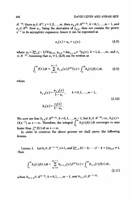
LEMMAI. Letb~~A(-‘-‘~,Irl,andZ~~,l(l-l)~~~(Z-k+l)pk,,Z~. Then
j”b,(t)f(t)dt=m$lb x k=O
r+l,k(r)Pk’(x)+~mb,+l(t)f(t)~~7
(2.11)
whem bl+i,k E A(k--[) k =O , 1 , ,.*a, m - 1, and br+lE A(+‘).
Two New Classes of Nonlinear Transformations 183
PROOF. Substituting (2.1) in /,” b,(t )f(t) dt and using the procedure that led to (2.6), we obtain
where
u,+,,k(X)= j=&-l)i+k[b,(*)p,(r)](f-k-l~> k=O,l,...,m-1,
(2.13)
%+1(x)= k~l(-l)k[b,(r)pk(~)l'L'.
The conditions lim, _ o3 p~-‘)(~)f(~-‘)(x) = 0, k = i, i + 1,. . . ,m, i =
1,2,..., m, that were imposed previously are sufficient for (2.12) to be true for all 121, since they also imply lim,,,[bl(X)Pk(X)](i-‘)f(k-i)(X)=O, k=i, i +1,..., m, i=1,2 ,..., m, which are sufficient for (2.12) to hold.
Now al+l,k E #--I) k =o 1 m - 1, and al+,
A(-[-‘) and Z+E A+ we ;an$-fte E AC-l-‘). Since CZ~+,E
%+1(x)= %+,hW+ cl+lw (2.14)
with aI+,=X~=:=,Z(Z-l)...(Z-k-tl)p,,, and c~+~EA(-‘-~). Since by as- sumption (Ye+ 1 # 1, we obtain (2.11) with
k=O,l ,..a, m-l,
(2.15)
b,,,(r)=~, If1
so that b 1+1 k~ Ack-‘) and bl+lE A(-‘-2), thus proving the lemma.
Starting now with Equation (2.9), with al,,(x), k=O,l,..., m-l, u,(x), al, c,(r), b,, k(r), k =O, 1,. . . , m - 1, and b,(x) already defined in (2.7), (2.8), and @lo), and assuming that Zr=r Z(Z - 1) . * * (1 - k + l)p,,, # 1 for Ia 1,
184 DAVID LEYIN AND AVBAM SIDI
we use Lemma 1 to define recursively a,,, k(x), k=O,l,...,m-1, al+,(x), aI+n cl+r(x), bl+,,Jx), k =O, 1,. . . ,m - 1, and &+,(x), Z= 1,2,. . . ,n - 1, by Equations (2.13), (2.14), and (2.15). We then sum Equation (2.9) and
/ mbr(t)f(t)dt=m&l
x k=O
1=1,2 ,..,) n-l, (2.16)
which are obtained by repeated application of Lemma 1. The result is
jrnf(t)dt = m~la;(z)f(k)(x)+j~b,(t)f(t)dt, (2.17) r k=O x
where
&b)= i bl,k(x), k=O,l,..., m-l. (2.18) Z=l
In (2.17) &‘E dk+‘), k =O,l,. . . ,m - 1, and &E A(-n-l). Let the asymp totic series of pi(x) begin with the power xi,, Since p,~ A(l), i, <l. The condition lim x _ o. pl( x )f( x ) = 0 which was previously imposed implies that f(x)= o(xPil) as x + 00. Since b”(x)= O(X-“-~) andf(x)= o(C’l) as x + cc, the integral 1,” b,,( t )f( t ) dt is o( x-“-~I) as x + cc. If we now choose n and x large enough, we can neglect 1,” b,,(t)f(t) dt in (2.17) and still get a good approximation to S = ja”f( t) dt; i.e., we can approximate S as
dt + m&?;(X)f(k)(X). k=O
(2.19)
Of course, in (2.19) one has to compute the functions j?;(x), k =O, 1,. . . , m - 1. But the computation of these functions becomes difficult, as is seen from Equations (2.18), (2.15), (2.14), and (2.13). However, as we shall show below, we can still make use of (2.19) to derive a transformation that will produce a good approximation to S.

Two New Classes of Nonlinear Transf~tions 185
SillCt!
Bk”(X)=Bkn-l(X)+b,,k(X)Y k=O 1 , ,***, m -1, (2.20)
and b,, k~ A(k--n+l), we can write
s;(X)=Xk+l B;,o+++F$2+ :.. +kL+qy,I 1 as x+00, k=O,l ,...:m-1, (2.21)
where the coefficients &, j=O,l,...,n, are the same for all &(x), k= 0, 1,. . . , m - 1, with 1) n. Therefore, we deduce from (2.17), (2.21), and the fact that j,” b,,+,(t)f(t)dt =o(~-“-~-~l) as x + 00 that j,“f(t)dt has a true asymptotic expansion which is given as
In many cases it occurs that the asymptotic series of r)k(x), k = 1,2,. . . ,m, do not all start with the power xk; ’ i.e., some may start with the lower power of x. We then assume that, in general, pkE Acik), ik G k, k = 1,2,. . . ,m. If one now follows the steps that led to (2.17), one can see that some of the /Y$, k=Ol , , . . . ,m - 1, may have asymptotic series which do not start with xk+‘, but with a lower integer power of x, say xtt. For example, if pkE A(‘), k=12 , ,... ,m (which for instance, with m = 2, is the case for Bessel’s equation), then from (2.7)-(2.17) one can see that a,, kE A(-‘+‘), k = 01 , ,***, m - 1, a, E A(-“-‘), and hence CQ = 0, b,,, E alsk, k = O,l,. . . ,m - 1, and bl-a,,Z=1,2... . Therefore, /$E A(‘). In general, &‘E A(“), with ik integers and jk S k -I- 1, k = 0, 1, . . . , m - 1. Actually, pi(x) = O(b,,,(x)) as x+00; hence from (2.7) jk~max(ik+l,ik+2-l,...,im-m+k+1), k= 0, 1, . . . , m - 1. Therefore (2.22) can be replaced by
We can summarize ah that has been said so far in the following theorem.

186 DAVID LEVIN AND AVFUM SIDI
THEOREM 1. Let f be integrable on [0, co) and satisfy the linear m&order diff&x&iul equation f(x)=& P~(x)~‘~)(x) with pkE dik), ik G k, k = 1,2,..., m. Zflim,,, pf’-‘)(x)f’k-‘)(r)=O, k=i,i +l,..., m, i=1,2 ,..., m, and if for any integer 1 2-l we have Zr=‘=,Z(Z-l)...(Z--k+l)p,,,#l, where pk.0 =lir&,x-‘p,(x), then, as X -00, j,“f(t)dt has an asymptotic expansion of the fomz (2.23) with jk Gmax(ik+r, ik+a - 1,. . . ,i, - m + k + 1), k=O,l,..., m-l.
We note that the conditions stated in Theorem 1 are sufficient. In ah the examples done by the authors ah of these conditions were seen to hold simultaneously. Therefore, the authors feel that the result (2.23) of Theorem 1 might hold even with a smaller number of conditions.
We note in passing that if f satisfies (2.23) such that &a # - 1, then f is in B(“‘). This can be proved by differentiating both sides of (2.22).
Having established (223, we now define our D-transformation. Following Schucany, Gray, and Owen [2] .and Levin [5-71, we demand that the
approximation Q$,,. ,n,_, to S=/Ff(t)dt satisfy the N=l+Zr~~n, equations
Dlzont)n,,...,*m_, = J (1 ,‘f t dt+m$f(k)(xl)xp *k-l p
k=O
2 -$, i=O
1=1,2 ,..., N, (2.24)
with & constants and x1 chosen to satisfy OC x1 < x2 <. . .<xN. The equations (2.24) form a linear set in N unknowns, namely, D,$~)n,,,,,,,_, and
pk$ i=o$l ssse) n,-1, k=O,l ,a.., m - 1, and can, in general, be solved for the N unknowns. DA’$,,, ,.,n,_l is expected to be a good approximation to S; however, the coefficients BkBk. i do not have to be identical to the &., i in (2.23), since the asymptotic series in (2.23) are usually infinite. As it turns out, the choice of the xI is important, and this point has been investigated by the second author; see Note Added in Proof. For the sake of simplicity, however,
\ we choose
xl=[+(z-l)r, 1=1,2 ,...,N, 5~0, 7~0.
Following Gray, Atchison, and McWilliams [l], we then denote D,!$)n,,,,,,,_,
by D::‘,,,...,,,_,[F(E); 1 h T w ere F(E)= /t f(t)dt. Usually it is more conve- nient to use the “diagonal” transformation DC”) n,n,...,n [F(6); -T] = D(“‘)[ F(t); 71. For the case m =2 and j. = ji ~0, which occurs frequently, Di”[ F(5); T] is given below:
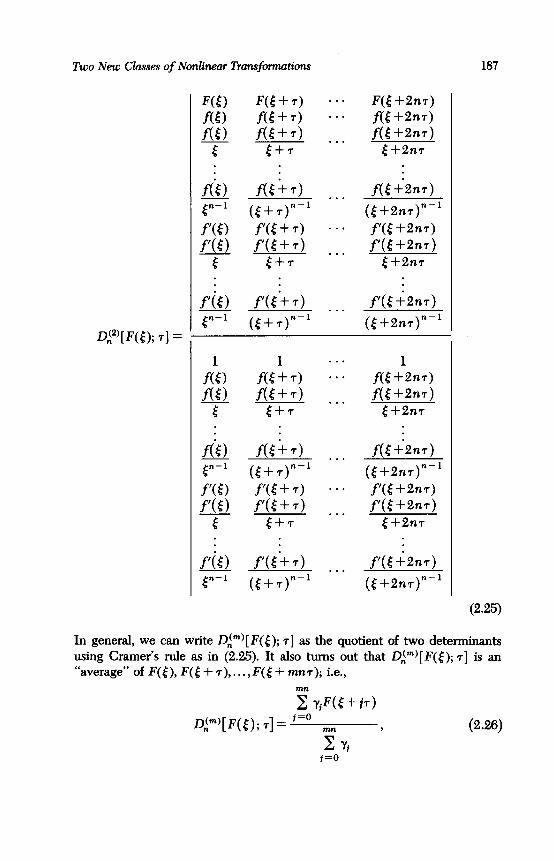
Two New Classes of Nonlinear Transjbrmations
F(5) F(5 + 7) f(5) f(t+r) f(E) fG+4
5 5+7
I: :
fis) f&d
D;2’[W); ?I= , En-’ (t+ 7)-l
fib f(5)
5
Ai) En-’ f(6) flo
E
A&) (5+ ry-1 fY5 + 7) f% + 4
t+r
f(i+ 4 ([+ry
. . .
. . .
. . .
. . .
. . .
. . .
. . .
. . .
. . .
. . .
. . .
. . .
. . .
. . .
F(t +2nr)
f(5+2nr) f(5 +2nr)
t+2nr
fY6 +2n71 fG +274
5+2nr
f(E :w ff E+2nr)
[+2nr
f(5 +2n7) ((+2nr)“-’
f(t +2nr) 05 +2nr)
5+2nr
f([ +2nr)
([+2nr)“-’
187
(2.25)
In general, we can write D,, (*)[ F(t); r] as the quotient of two determinants using Cramer’s rule as in (2.25). It also turns out that Di”)[F([); r] is an “average” of F(t), F(t + r), . . . ,F([ + mnr); i.e.,
2 y,F(t + id D;“)[F(t); r] = ‘=’
%j ’
(2.26)
i=O

188 DAVID LEVIN AND AVFiAM SIDI
where y, are the cofactors of F(E + jr) and are dependent on f(x), f(x), . ..,f(“-‘j(x), Therefore, the Dtransformation can be viewed as a nonlinear summability method.
3. SOME SPECIAL CASES OF THE D-TRANSFORMATION AND AN EXTENSION OF THE CONFLUENT E-ALGORITHM
For m = 1 and j,, =O the system of equations (2.24) reduces to that given by Levin [7] in his development of the P-transformation. Hence the D!$trans- formation is identical to the P-transformation of Levin. The P-transformation has been developed for functions of the form f(x)= eiwxh(x) with w constant and h E Acy), y (0. It is not difficult to show that these functions satisfy first-order linear differential equations of the form f(x)= p(x)f(x) with p(x)=[h’(x)/h(z)+iw]-‘, so that pi A”), which implies that j. =O in (2.23). It is worth mentioning that the P-transformation has worked very efficiently on the Bromwich integral, which is used in inverting Laplace transforms. This fact may indicate that the Dtransfoxmation would also produce very good results.
If the asymptotic expansion (2.23) turns out to be finite, i.e.,
(3.1)
thenS=l,“f((t)dt~D~~),;,,,,,~~_,[F(5);7]foralln;,nk,k=O,l,...,m-1, 5 > 0, and r > 0. As an example of (3.1) we can consider the Bessel functions of the 1st kind of odd order, namely, _lak+i(x), k = 0,1,2,. . . . Using the relation [IS]
J m.hk+l(t)dt = &(x)+2 ii J,Zb), ?z I=1
together with the different recursion relations between the Jl, we finally arrive at (3.1). For k = 1 (3.1) becomes
As another example we can consider the functions which satisfy linear
Two New Claws of Nonlinear Transformations
differential equations of the form
f(x)= g $ c& f’k’(X). i I k=l f=O
189
(3.2)
Then we can see from (2.7) that al(x) is a constant; hence b, ~0, and b,, k(~) are polynomials of degree k + 1, k ~0, 1, . . . , m - 1, i.e.,
/ f(k)(X). (3.3)
x
If&(x), k=l,2 ,..., m, in (2.1) are constants, then b,,k(x), k =O, 1,. . . ,m - 1, in (2.3) are constants too, and hence Dim’ with ik = 0, k = 0, 1, . . . ,m - 1, Iike the G,-transformation and the csrn in the confluent ealgorithm, integrates exactly functions which satisfy linear m&order differential equations with constant coefficients.
We can make use of (3.3) to obtain another transformation which will integrate exactly functions which satisfy equations of the type (3.2). We start by writing (3.3) as
(3.4)
and differentiate this equation M = m( m + 3)/2 times to obtain a total of M+l equations for the M+l constants S=j,"f((t)dt and &I, i=O,l,...,k
-t-l, k=O,l , . . . , m - 1. We now define the Gtransformation for any integra- ble function f. We demand that the approximation Cc”) to S, satisfy the
M + 1 equations
f(kw 1 =o,
i-0,1,... ,M, (3.5)
where &, are constants. Equations (3.5) can, in general, be solved for the M-t-l unknowns C(*)=C(“)[F(x)] and&i, j=O,l,..., k+l, k=O,l, . . . . m
- 1. Obviously C(“‘)[F(x)] E S if f satisfies (3.2). It is easy to see that the
190 DAVID L&YIN AND AVRAM SIDI
C-transformation is an extension of the confluent e-algorithm of Wynn, since this algorithm can be obtained by solving the set of equations
d’
dx’
for earn.
m-l
I =o, i-O,1 ,..., m+l, (3.6)
4. APPLICATIONS OF THE D-TRANSFORMATION
In this section we shall illustrate the use of the LXtransformation that was developed in Section 2 for several functions which are in I?(‘) and 13c3). The integrals of all those functions considered in this section converge very slowly. The high-order Gtransformations work efficiently on some of these functions but fail to work on most others.
It is worthwhile to make a few comments on the practical application of the D-transformation. In order to be able to apply the IFtransformation efficiently one has to know (1) the smallest possible positive integer m such that the integrand f is in B(“), and (2) the parameters jk, k =0, 1, . . . ,m - 1, in the asymptotic expansion of j,“f(t ) dt. If the upper bounds for the jk are known, then we can substitute these upper bounds for the jk in the equations (2.24). If the differential equation that f satisfies is not readily obtained, then we proceed as follows: Since integrability of f at infinity means that lim x_m/pf(t)dt =O, we must have
lim Xfqk)(X)=O , k=O,l,..., m-l, (4.1) r-+00
in the asymptotic expansion in (2.23). Therefore, we replace jk in (2.24) by the minimum (rk of k + 1 and s,., where sk is the hrgfi!St of the integers s for which lim X#c~f(~)(X)=O. If, with jk replaced by uk, the first few coeffi-
cients, say &,a, &, 1,. . . , Pk, ,ky in (2.24), turn out to be very small compared with the rest of the coefficients, then we can assume that jk = ‘Jk - rk in (223) and replace jk by ok - rk in (2.24); and if indeed jk = uk - rk, then we are likely to obtain better accuracy for the approximations to S = jcf(t ) dt using the same number of the F(xi).
We shall now state a lemma that will be useful in determining the order of the differential equations that the function f whose integral is to be evaluated satisfies.

Two New Classes of Nonlinear Transformations 191
LEMMA 2. Zf the finctions f and g satisfy linear dij$rential equations of order m and n respectively, then their product fg and their sum f + g, in general, satisfy linear diffkrential equations of orders less than or equal to mn and m + n respectively.
PROOF. Let f and g satisfy
f = 5 Pkf? k=l
g = i qlg’? I=1
(4.2a)
(4.2b)
Multiplying (4.2a) and (4.2b), we get
fg = $! i pkqlf(k)d’)* k=l I=1
(4.3)
In (4.3) we have to be able to express the mn products f (k)g(z), k = 1,2,. . . , m,
2=12 , ,***, n, as linear combinations of (fg)“), r=1,2,...,mn. Using Leibnitz’s rule for differentiating the product of two functions, we have
(fg)“) = ,4 (;)f’s’g”-s’, r =1,2 ,...,mn. (4.4)
In (4.4) if s =O, f(“) is replaced by zr=i pk ftk’ using (4.2a), and if s > m, then f’“) is expressed as a combination of f, f’, . . . , f cm), by differentiating (4.2a) s - m times. The same can be done for g(‘-‘) when r - s =O and r--S>n. Then we wih have expressed (fg)“), r=1,2,...,mn, as combina-
tionsof themnproductsflk)g(‘), k=1,2 ,..., m, 2=1,2 ,..., n; i.e.,
(fg)@‘= 2 i A,,f@‘g”‘, 7 =1,2 ,...,mn. (4 -5) k=l I=1
Now (4.5) is a set of mn linear equations in the mn unknowns f@)g(‘), k=1,2 ,..., m, 1=1,2 ,..., n, and can, in general, be solved to give flk)g(‘) as

192 DAVID LEVIN AND AVRAM SIDI
linear combinations of (fg)“), T = 1,2,. . . ,mn. Hence (4.3) becomes
fg = 5 A,(fg)('). r=l
For the case off + g we add (4.2a) and (4.2b) to obtain
f+g= i pffk’+ f: t&g”‘.
(4.6)
(4.7) k=l I=1
In (4.7) we have to express fck), k=1,2 ,..., m, and g(l), 1=1,2 ,..., n, as combinations of (f + g)(‘), r = 1,2,. . . ,m + n. Using (f + g)(‘) = f (‘) + g(‘) and the fact that for T > m f(‘) can be written as a combination of f’,f” ,...) f’“‘, and for r > n g(‘) can be written as a combination of g’,g”,...,g (n), the result follows as in the previous case; i.e.,
m+n
f+g= 2 Mf+gP. (4.8) r=l
COROLLARY 1. Zf f satisfies a linear diffkrential equation of order m, then, in general, f 2 satisjb a linear differential equution of order m(m + 1)/2 or less.
PROOF. The proof follows from the fact that the number of unknowns ftk)g(‘) in (4.3) is m(m + 1)/2 when f = g.
COROLLARY 2. Zf the coefj%ients p,, k = 1,2,. . . ,m, and Q~, I= 1,2,. . . , n, have asymptotic expansions in inverse powers of x as x 3 00, then so do A,, r=l,2,..., mn, in(4.6)andB,, r=1,2 ,..., m+n, in(4.8).
COROLLARY 3. Zf fE Z3 (m) and g E ACT) or g(x)= eux, then fg satisfies a linear differential equation of order m or less with coeficients that have asymptotic expansions in inverse powers of x as x + 00.
The proofs of these corollaries are easy and we omit them. From the experience gained in the use of the P- and high-order G-transfor-
mations, we expect that as n tends to infinity, D,$“)[F(t; T)] should tend to

Two New Chsar of Nonlinear Transfmtions 193
j,“f(t)dt quickly if fE B(“) and satisfies all the conditions of Theorem 1. The numerical results in the following examples indeed confirm this. Conver- gence properties of the D-transformation have been taken up by the second author in a separate paper, see Note Added in Proof.
EXAMPLE 4.1.
z= I m sint
0 -i-dt =; =1.570796326795... .
The integrand f(t)=(sin t)/t is integrable at infinity and satisfies the differential equation f = -(2/t)f’- f”; hence it is in IS(‘). Therefore, we expect 0, c2) to work efficiently. Also since sin t satisfies a second-order linear differential equation with constant coefficients, we expect G,, to work effi- ciently too. This point has been mentioned in the introduction. From the differential equation that f satisfies we see that j,, < - 1 and jr ~0. However, we used the prescription proposed for the case in which the differential equation is not known explicitly, and in (2.24) we replaced j. by a0 =O and jr by ur =O, where ok = min(k -I 1, Sk), k =O, 1. Accordingly Di2)[ f(t); 71 was computed by solving the 2n + 1 linear equations
with [=l and r = 1, and F(r)= _j$‘[(sin t)/t] dt. The finite integrals F(< + jr) were computed correctly to 14 decimal points using a Gauss-Legendre quadrature formula. We also computed G,,[ F(5); r)]. The results of the computations with IIA2) and G,, are given in Table 1. Di2)[F([); r] has been compared with G,,[F(t); r], since they both use the same finite integrals, namely, F([+ j7), j=O,l,..., 2n.
For the integral /,“[(&I t)/ t] dt we have the asymptotic expansion
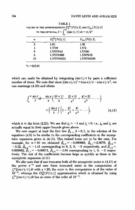
194 DAVID LEVIN AND AVRAM SIDI
TABLE 1 VALUES OF THE APPROXIMATIONSm~,?[ F(1); 11 AND G,,[ F(1); 1]
TO THE INTJZGFtAL I= /
[(sin t>/t] dt = n/2” 0
n D@)[ F(1). l] n > G,, [ F(l); 11
2 1.63 1.56 4 1.5716 1.572 6 1.5707943 1.57080 8 1.57079 606 1.57079 55 10 1.570796323 1.57079 6326
*n = 2(2)10
which can easily be obtained by integrating (sind)/t by parts a sufficient number of times. We note that since [(sin x)/x ]‘=(cos x)/x -(sin x)/x2, we can rearrange (4.10) and obtain
J -- . . . x
sin x ’ +- ( H p2’+41-
X X2 X4 *** ’ )
(4.11)
which is in the form (223). We see that j. = - 1 and jr ~0; i.e., j. and jr are actually equal to their upper bounds given above.
We now expect at least the first few pk, i, k =O, 1, in the solution of the equations (4.9) to be similar to the corresponding coefficients in the asymp- totic expansion given in (4.11). This indeed turns out to be the case. For example, for n =lO we obtained &o = -0.000068, & ~2.0076, go,2 = -0.32, &a= - 1.41 corresp+iing to 0, 2, 0, -8 respectively, and &o = 0.999982, Pr, r = -0.m71, /31,2 = - 1.84 corresponding to 1, 0, -2 respec- tively. The rest of the coefficients become large as quickly as those in the asymptotic expansion (4.11).
We also note that if one truncates both of the asymptotic series in (4.11) at th e power XC9 and uses these truncated series in the computation of /,” [(sin t )/t] dt with x =20, th e error in this computation is of the order of lo-‘, whereas the Df$[F(l); I] approximation which is obtained by using /;‘[(sint)/t] dt h as an error of-the order of 10Vg.
Two New Classes of Nonlinear Tramfmtions 195
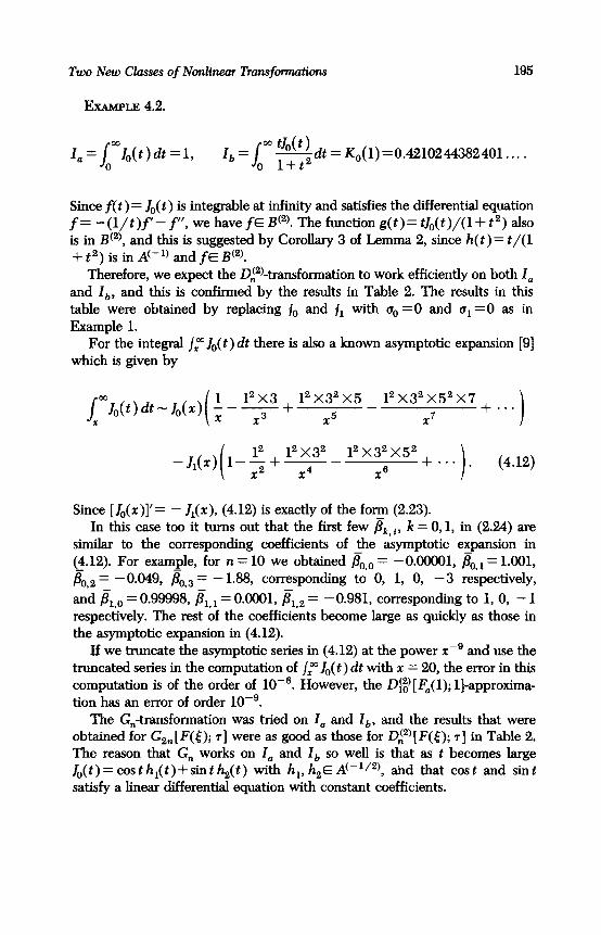
EWLE 4.2.
I, = /
mJO(t)&=l, I = m %W
0 b l ---&dt=K,(1)=0.4210244382401....
Since f( t ) = J,(t) is integrable at infinity and satisfies the differential equation f=-(l/t)f-f”, wehavefEB . (2) The function g(t)= tJ,(t)/(l+ t2) also is in Bc2), and this is suggested by Corollary 3 of Lemma 2, since h(t) = t/(1 + t2) is in A(-‘) and fE B(‘).
Therefore, we expect the DA2)-transformation to work efficiently on both I, and I,, and this is confirmed by the results in Table 2. The results in this table were obtained by replacing j0 and jl with a0 =O and u1 =O as in Example 1.
For the integral 1,” J$ t) dt there is also a known asymptotic expansion [9] which is given by
p&)&_Jo(x) g2jz+ 12x;y _ 12x32x;52x7+ . ..) x (
-&(x)(1-$+y- 12x~;x52 + .j. (4.12)
Since [l,(x)]‘= - II(x), (4.12) is exactly of the foe (2.23). In this case too it turns out that the first few &, i, k = 0, 1, in (2.24) are
similar to the corresponding coefficients of the asymptotic expansion in ($12). For exam_ple, for n = 10 we obtained &, = -0.00001, /$I = 1.001, &, = -0.049, &, = - 1.88, corresponding to 0, 1, 0, - 3 respectively,
and &.o = 0.99998, &I = 0.0001, &2 = -0.981, corresponding to 1, 0, - 1 respectively. The rest of the coefficients become large as quickly as those in the asymptotic expansion in (4.12).
If we truncate the asymptotic series in (4.12) at the power x? and use the truncated series in the computation of 1,” JO( t ) dt with x = 20, the error in this computation is of the order of lo-*. However, the D$)[ F,(l); ll-approxima- tion has an error of order 10W9.
The G,,-transformation was tried on I, and I,, and the results that were obtained for G,,[F(E); T] were as good as those for Di2)[F([); 71 in Table 2. The reason that G,, works on I, and I, so well is that as t becomes large J,(t)=costh,(t)+sinth2(t) with h,,hz~A(-1/2), tid that cost and sint satisfy a linear differential equation with constant coefficients.

196 DAVID JXVIN AND AVRAM SIDI
TABLE 2 VALUES OF THE APPROXIMATIONS oi2’ [ F,( 1); l] AND oA2’ [ Fb( 1); 11
TO&= / 0
~JO(t)dtANDzb=jm t&( t)/(l + t 2, dt RESPECTIVELY a 0
n D:2qF,W; 11 DC2’[ F,(l);11 n
2 1.04 0.43 4 1.003 0.4212 6 0.999994 0.421027 8 0.9999998 0.421024433 10 0.9999999986 0.421024434 12 0.99999999984 0.4210244382407
“For n = 2(2)12, where F,(r) = /; J,,(t) dt and Fb(z) = /o” tJ,(t)/(l+ t2) dt.
The integrals I, and I, were computed also by L.&n [6] using a transfor- mation designed to work exclusively on integrals of the form
@)JV(t) dt, hi A(v),
and very good results were obtained.
where
C(z)=~‘_s( tt2) dt and S(x)=Jo”sin( it”) dt.
Two New Classm of Nonlinear Trutasfmtions 197
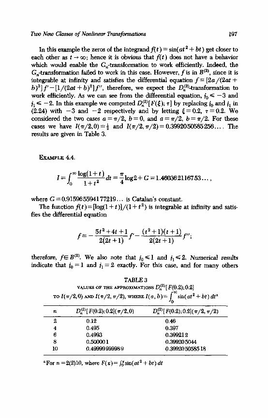
In this example the zeros of the integrand f(t) = sin(at2 + bt ) get closer to each other as t --) co; hence it is obvious that f( t ) does not have a behavior which would enable the G,,-transformation to work efficiently. Indeed, the G,-transformation failed to work in this case. However, f is in Bc2), since it is integrable at infinity and satisfies the differential equation f= [2~/(2at + b)3] f - [l/(2& + b)‘] f’, therefore, we expect the D,$2)-transformation to work efficiently. As we can see from the differential equation, j. G -3 and jl < - 2. In this example we computed Di2)[F([); 71 by replacing j0 and jl in (2.24) with -3 and -2 respectively and by letting [ = 0.2, T = 0.2. We considered the two cases a = r/2, b = 0, and a = r/2, b = n/2. For these cases we have Z( n/2,0) = f and Z( 7r/2,7~/2) = 0.3992050565256.. . . The results are given in Table 3.
EXAMPLE 4.4,
z = lW ‘““,‘:y’ dt=~log2+G=1.460362116753... ,
where G =0.915965594177219.. . is Catalan’s constant. The function flt)=[log(l+ t)]/(l+ t2) is integrable at infinity and satis-
fies the differential equation
therefore, fE B (2! We also note that i0 91 and jl G2. Numerical results indicate that j0 = 1 and jl = 2 exactly. For this case, and for many others
TABLE 3 VALUES OF THE APPROXIMATIONS oA2’[ F(0.2); 0.21
TOl(lr/2,0)hm,I(n/2,?r/2),~eREI(a,b)=lomsin(ot2+bt)dt”
n D~2’[F(0.2);0.2](~/2,0) Di2'[ F(0.2); 0.2]( 7r/2, n/2)
2 0.12 0.46 4 0.495 0.397 6 0.4993 0.399212 8 0.5mOOl 0.399205044 10 0.49999999989 0.39920 50585 18
“For n=2(2)10, whereF(x)=jtsin(~t~+bt)dt

198 DAVID LEVIN AND AVFL4M SIDI
which contain logarithmic terms multiplied by functions in A(u), the choice of the xi, j=1,2 ,..., N, in the equations (2.24) becomes very important. If we choose the zi equidistantly as in the previous examples, the approximations DA2)[ F(t); T] are poor for large n. If we choose xi = [&i)‘, j = 1,2,. . . , N, then the convergence of the approximations Di2’ obtained by solving the equations (2.24) improves considerably. In our computations we chose 5 = 1 and r = 0.2. The results of the computations are given in Table 4.
We note that the G,,-transformation failed to work in this case.
EXAMPLE 4.5.
q( y2 dt = ; = 1.57079 6326795.. . ,
The integrandf(t)=[(sin t)/t] 2 is integrable at infinity, and since (sin t)/ t is in IS(‘) from Example 4.1, [(sin t)/t12 satisfies a differential equation of order 3 or less with coefficients in A (y) for some values of y, according to Corollaries 1 and 2 of Lemma 2. Indeed, f satisfies the differential equation
hence fE Bc3). Therefore, we except the D~3)-transformation to produce good results. The G,-transformation does not work efficiently on this function, although (sin t)2 satisfies a linear differential equation of order 3 with constant coefficients. The parameters jkr k =O, 1,2, in (2.24) satisfy jc, < 1, ii GO, j2 G 1, and from numerical results it turns out that j0 = 1, ji =O, j2 = 1. In the
TABLE 4 VALUES OF THE APPROXIMATIONS 0;" TO
I= mhdl+t)dta / 0 1+t2
n D’2’ n
2 1.14 4 1.46085 6 1.46042 6 1.46036208 10 1.4603621191
“Obtained using xi = e(i-‘p.‘, j = 1,2 ,..., N, for n =2(2)10
Two New Classes of Nonlinear Transfmtions 199
TABLE 5
n Dc3’[ F(1). l] ” 9
2 1.61 4 1.5799 6 1.570793 8 1.57079635 10 1.57079932688
‘For n =2(2)10.
computation of Q3’ we assumed that the equation was not known and replaced jk by uk =min(k + 1, sk), k =O, 1,2, which in this case turned out to be equaI to 1. The approximations Di3)[ F(t); r] to Z were obtained by using E = 1 and r = 1. The results of the computations are given in Table 5.
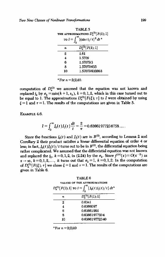
bAA@LE 4.6.
z= J 0
mZo(t)l,(t)~=~=0.63661977236758....
Since the functions Jo(t) and Zi(t) are in Bc2), according to Lemma 2 and Corollary 2 their product satisfies a linear differential equation of order 4 or less; in fact, Jo( t )Zr( t )/t turns out to be in Bc3), the differential equation being rather complicated. We assumed that the differehtial equation was not known and replaced the jk, k =O, 1,2, in (2.24) by the uk. Since flk)(r)= 0(xd2) as x+00, k=0,1,2 ,.a., it turns out that uk = 1, k = 0, 1,2. In the computation of ZP’[F(5); ] r we chose [ = 1 and r = 1. The results of the computations are give: in Table 6.
TABLE 6 VALUES OF THE APPROXIMATIONS
DL3’ [ F( 1); l] TO I = / o%wJdwtl &”
n DA3’[ F(1); l]
2 0.6341 4 0.63660 97 6 0.63661991 8 0.63661977204 10 0.636619772340
aFor n =2(2)10
200 DAVID LEYIN AND AVRAM SIDI
We note that the G,,-transformation failed to work in this case too. Di3)[F(6); l] was compared with G3n[F([); r]. Gsc,[F(l); l] was seen to be correct to 5 decimal places, and F(31) was seen to be correct to 3 decimal places.
5. THE d-TRANSFORMATION FOR INFINITE SERIES
Let BCrn) be the set of infinite sequences {f(r)} whose elements f(r), r =1,2,3 ,..., satisfy linear mthorder difference equations of the form
f(r)= k~lr44AkfG93 (5.1)
where A’f(r)=f(r), Af(r)=f(r+l)-f(r), A’f(r)=A[Af(r)], etc., and ;k.)2considered as functions of *the continuous variable x, are in A@),
, )..., m. In this section we are going to make use of the ideas that were developed
in Section 2 to derive the d-transformation that will give good approximations to the sums of infinite series of the form X:&f(r), where {f(r)} E @‘“). In essence the d-transformation is the discrete analogue of the D-transformation for infinite integrals.
In analogy to Theorem 1 for infinite integrals whose integrands are in Rem), we now state Theorem 2 for infinite series whose associated sequences are in B(m)*
THEOREM 2. Let IZ~=“,,f(r)l<co, and Z&f(r), r=l,2 ,..., satisfy the linear mth-orderdiff&nce equutionf(r)=I&pk(r)Akf(r) with pk~ACik), i,~k, k=1,2 ,..., m. Zf
rlifnm [A’-‘pk(r)][A’k-if(r)] =O, k=i,i+l,..., m, i=1,2 ,..., m,
(5.2)
and
2 Z(Z-l)+Z-k+l)p,,,#l, 12-1, Zinteger, (5.3) k=l
whew pk.0 =&,, rekpk(r), then ZTzo=, f(r), for R + 00, has an asymptotic
Two New Classes of Nonlinear Transfmtim !201
expansion of the fm
5 f(+y*y(R)Rfr. j3k,o+++%+ . ..) (5.4) r=R k=O
with jk &m&i,+,, ik+s -l,...,i, -m+k+l), k=O,l,..., m-l.
The proof of this theorem is analogous to that of Theorem 1 of Section 2 with D E d /dx replaced by A, 1,” replaced by ZTEo=, , and integration by parts replaced by “summation by parts” using the formma
$Rg(r)Ah(r)=-g(R-l)h(R)+g(R’)h(R’tl)
- 5 [Ag(r-l)]h(r). r=R
(5.5)
In order to show the similarity of the proof of Theorem 2 to that of Theorem 1, we give the first step of it in detail, the rest being analogous.
Summing f(r)=Zrcl pk(r)Akf(r) from r =R to infinity and using (5.5) repeatedly together with the conditions in (5.2), we obtain analogously to
(2.6)
g flr)=~~~%k(R)AkflR)+ r~Radr)ft~h (5.6) r=R
where
a,,k(R)= i (-l)‘+kA~-k-lq(R-f+k), k=O,l ,.a., m-l, j=k+l
al(r)= i (-l)kAkpk(r-k), TZ=R. (5.7)
k=l
We now use the fact that if hE Acy) [i.e., h(r)= horr+ O(rr-l) as r --$oo], then Ah(r)=yhOr y-l + O(rym2) as r -+ 00, i.e., AhE A(?-‘); and if hE A’o’, then Ah E tie2). This property of the difference operator A is similar to that ofthedifferentialoperatorD.Wethenseethata,,kEA(k+1),k=O,1,...,m- 1, and a,E A(o, and is of the form
q(r)= a1 + q(r), (54
202 DAVID LEVIN AND AVRAM SIDI
where a1 = Zp=r,( - l)kk!p,,, and C,E A(-‘). Since (or # 1 according to the hypothesis stated in the theorem, (5.6) can be written as
where
a1 k(R) h,kw= l_ar’ k=O,l,..., m-l, 1
(5.10)
b,(r)=+@, rz=R, 1
and where b, kE Ack+‘), k =O, 1,. . . , m - 1, and b,~ AcP2). Since f(r)= o(1) and b,(r)= O(rP2) as r + co, the sum ZyTO=Rbl(~)f(r) converges to zero faster than the sum IZ~&f(r) as R + cc.
We now make use of (5.4) to derive the d-transformation for infinite series. We demand that the approximation dkr,‘n,,.,.,,__, to S =Zr=rf(r) satisfy the N = 1+2&’ nk equations
1=1,2,..., N, (5.11)
with & constants and R, chosen to satisfy OG R,< R,< . . . <RN, and with 2:: r f(r) =0 when R, = 0. The zquations (5.11) form a linear set in N unknowns,namely,d~~~ “,,,,,, ,__,and~k,i,i=O,l,...,nk-l,k=O,l ,... ,m-- 1, and can, in general, be solved for d$TJn,,,, ,,n,_,. Again for the sake of
simplicity we choose
Rl=[+(Z--1)q 1=1,2 ,..., N,
where 5 2 0, r 3 1 are integers. We denote dkT,),,,,,,,,__l by
dL;)n, ,..., .,_,[F(U; I. 7 w h ere F(t) is the sum of the first 6 terms of ZT=rf(r), i.e., F([)=Zf.-, f(r). We also define the “diagonal” d-transformation as d(“‘) n,n,....n [F(t); T] = d’“)[F(& T]. n
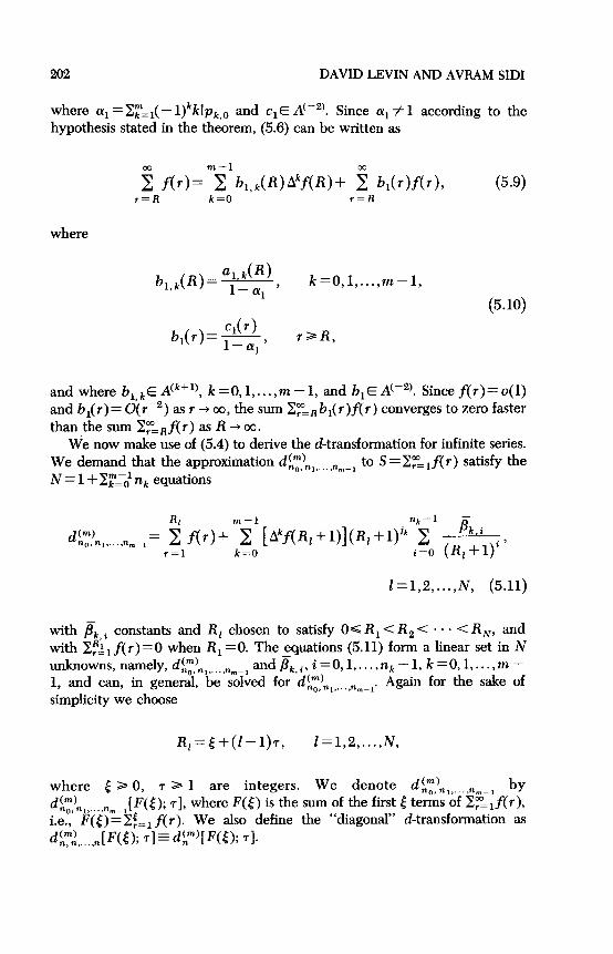
Two New Classes of Nonlinear Transf~tions 203
cl$,“‘)[ F( 0; l] for the case m = 2 and il = iz = 0, which occurs frequently, is given below:
@[F(5); l] =
F(E) F(.$+l) ..a F(t +2n)
f(E+l) f(E+2) ... f([+2n+l)
fG+l) f(E+2n+l) f(5 +2) . . . <+1 5+2 {+2n+l
f(h) f&2) f(<+in+l)
(E+l)“-’ @+2)“_’ **. (‘$+2n+1)“_’
Af(t+l) Af(5+2) a*. Af(t+2n+l)
Af(t+l) Af(E +2) . . . AI%$;~) E+l t+2 n
Af(i+O Af(i+2) Af(t+&+l)
(E+l)“-’ ([+2)“-’ *‘* (5+2n+l)“-’
1 1 . . . 1
f(E.+l) f(5+2) --a f(t+Zn+l)
xs’+i” f(l+2) f(5+2n+l) . . .
2+2 [+2n+l
f(c+l) f($ $2) f(c+in+l)
([+l)“-’ (t+2)“-’ *** (5+2n+1)“_’
Af(E+l) Af(5+2) a.- Af(.$+zn+l)
Af(E+l) Af(E+2) . . . AJT~~;;~) E+l E+2 n
Af(i+l) Af(i+2) Af(5+‘2n +l)
([+l)“-’ ([t-2)“-’ *** (<+2n+l)“-’ (5.12)
Like the Dtransformation, the d-transformation is also a nonlinear summabil- ity method.
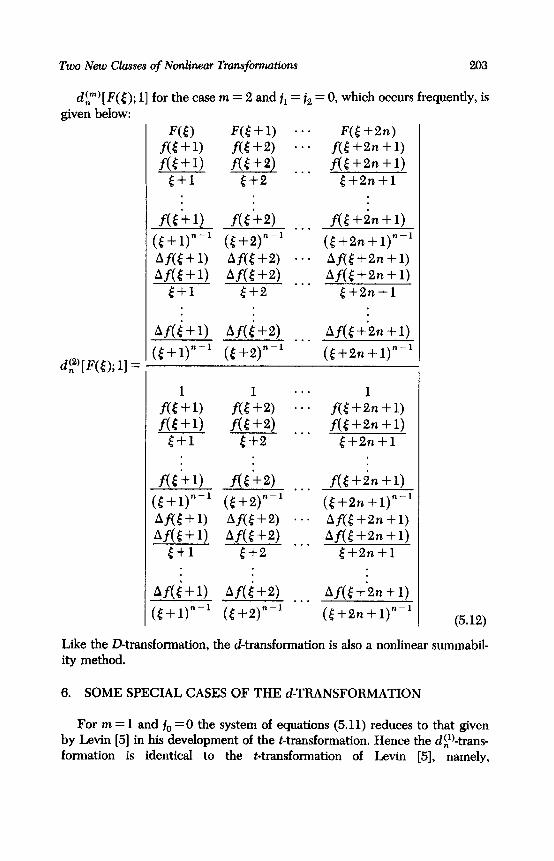
6. SOME SPECIAL CASES OF THE d-TRANSFORMATION
For m = 1 and j0 =O the system of equations (5.11) reduces to that given by Levin [5] in his development of the t-transformation. Hence the di’)-trans- formation is identical to the t-transformation of Levin [5], namely,
2804 DAVID LEXIN AND AVRAM SD1
d;“[F(~);l]=t,,[F(E+l)]. F or m = 1 and f0 = 1 the d~l)-transformation turns out to be identical to the u-transformations of Levin [5], namely dt)[F(E); l] 3 u,[F([ + l)] with n >l. The fact that the t- and u-transformations accel- erate the convergence of slowly converging series whose associated sequences are in B(l), in the sense that as n + co t,, and U, converge to the sums of the series quickly, indicates that the dim)-transformation will be as efficient as the t- and u-transformations when applied to series whose associated sequences are in BCm) for any m 21; i.e., as n --) CIO, dim) will tend to the sums of these series quickly. This was indeed the case in all the examples that were considered. (See Section 7.)
Italsoturnsoutthatd~“~[F(~);1]withj,=O,k=O,l,...,m-1,isidenti- cal to the e,,,[ F(t + m)]transformation of Shanks [8], which in turn is identical to eZm[ F(t)] of the e-algorithm of Wynn [3].
When the d-transformation is applied to power series, rational approxima- tions are obtained. From what has been said above we see that the rational approximations obtained using di”‘) with jk = 0, k = 0, 1, . . . ,m - 1, are just the Pad& approximants, and those obtained using din with j,, = 1 are the u- approximants of Levin [6], see also Longman [lo]. The Pade and u-approxi- mants have proved to be very efficient for power series whose coefficients satisfy simple recurrence relations. However, for power series whose coeffi- cients satisfy complicated recurrence relations of the form (5.1) we expect that the rational approximations obtained using the d(“‘)-transformation will be more appropriate. These rational approximations can be cast into a form which is convenient to use. For example, the dF)[ F( 5); l] approximation to a power series Z~?,lurrr-l, with i,, = jr = 0, after some elementary row and column transformations on (5.12), can be expressed as @[F(E); l] = N/D, where
N=
t+1
X2n 5: a,r”-l X2n-l 2 a,x’-l
r=l
at+1
at+1
E+l
at+1
([+l)“-’
at+2 at+2
5+1
r=l
at+2
at+2
t+2
. . .
. . .
. . .
. . .
. . .
. . .
. . .
6 f2n
I: a$-’
r=l
a&+zn+l
Uf+2n+l
t+2n+1
ac+2n+ 1
(5+2n +1)“_’
at+2n+2
at+2n+2
5+2n+1 (6.1)

Two Nm Classes of Nonlinear Transfmtions 205
and D is obtained from N by replacing the first row in the determinant expression in (6.1) with the row vector (x2n, x2n-1,. . . ,x, 1).
As is seen from (6. l), the rational approximation obtained using dr) [ F( t ); l] has numerator of degree 2n + [ -1 and denominator of degree 2n. In general, the rational approximations obtained using dim)[ F(t); l] with jk = 0, k=O 1 , ,***, m - 1, will have numerators of degree mn + E - 1 and denomina- tors of degree mn.
7. APPLICATIONS OF THE d-TRANSFORMATION
In many problems of applied mathematics the solution is obtained in the form of an infinite series Z~=ia(r)+~(x), where G,(X) are orthogonal poly- nomials, or elementary functions, or special functions, or products of them. Hence the functions +Jr) satisfy a linear recursion relation of some finite order hence the sequences {+,(x)} are usually in l8”‘) for some m. As we shall see below, if a(r) = t” or a E A(v) for some y, then in general, {a(r)$~Jx)} E B@Q too.
Several methods for accelerating the convergence of series of orthogonal functions have been developed in the past. Mention can be made of the methods of Maehley [ll] and Clenshaw and Lord [14] for Chebyshev series, of Holdeman [12] for series of orthogonal polynomials in general, and of Fleischer [13] for Legendre series. A recursive method for the computation of the approximations of Clenshaw and Lord has been given by the second author [ 151. All these methods are of the Pade type. We finahy mention the methods of Levin [6] for accelerating the convergence of series of orthogonal polynomials, which are like the d-transformation, but unlike the d-transforma- tion require full knowledge of the recursion relations that these polynomials satisfy. This point has been explained in detail in Section 1. One drawback of all these methods is that one needs different transformations for different kinds of series, whereas the same d-transformation can be used for all of these series. If the function represented by the infinite series in question is analytic, then the d-transformation, like the methods given in [ll, 12, 13, 141, can be used to analytically continue the series to regions in which the series diverges. This point is briefly illustrated in Example 7.1.
In this section we shall illustrate the use of the d-transformation on different infinite series of the form mentioned in the previous paragraph; in particular, we shall deal with series whose associated sequences are in B(‘) and B(4)*
The choice of the parameters jk in (5.11) is exactly as explained in Section 4 for the D-transformation with the derivative operator replaced by the forward difference operator A. In analogy to Lemma 2 and its Corollaries 1,2, and 3 of Section 4 we state
206 DAVID LEVIN AND AVRAM SIDI
LEMMA 3. Zf {f(r)} and {g(r)} satisfy linear dij@rence equations of orders m and n respectively, i.e.,
f(r)= i ~k(r)A~f(4 g(r)= i dr)A’gW, (7.1) k=l Z=l
thentheirproduct {f(r)g(r)} undtheirsum{f(r)+g(r)},ingeneruZ,satisji~ linear diff?ence equations of orders less than ur equul to mn and m + n respectively, i.e.,
f(r)g(r)= 2 Ak(r)Akk[f(r)g(r)ly k=l
m+n
f(r)+g(r)= Ix %r)@[f(“)+g(r)l.
U-2)
k=l
coRoILAFiY 1. Zf {f(r)] t E sa is es a linear difference equation of order m, then, in general, {[f(r)12} t’fze sa zs s a lineur di~erence equation of order m(m + 1)/2 or less.
COROLLARY 2. Zf the coeficients pk( r), k = 1,2,. . . ,m, and ql(r), 1 = 1,2,..., n, in (7.1) have asymptotic expansions in inverse powers of r as r--co, then so do Ak(r), k=1,2,...,mn, and &(r), k=1,2 ,..., m+n, in (7.2).
COROLLARY 3. Zf { f(r)} E g(m) and g(r)= tr or gE A(u) for some y, then the terms of the sequence {g( r)f(r)} satisfy a linear diffbence equation of order m or less with coeflcients that have asymptotic expansions in inve-rse powers of r as r -+ 00.
The proofs of Lemma 3 and its Corollaries 1,2, and 3 are identical to those of Lemma 2 and its corollaries if one uses
AN[f(r)g(r)]= 5 ( y)Nik( “ik)[A~-‘f(r)][Akt’g(r)l, (7.3) k=O j=O
in the same manner that Leibnitz’s rule for differentiating the product of two
Two New C/awes of Nonlinear Tranafonnatim 207
functions was used in Section 4. The formula given in (7.3) can be proved by induction on N.
EXAMPLE 7.1.
where P,(r) is the Legendre polynomial of degree r, r =O, 1,2,. . . . This series converges slowly for ( x 1 G 1 and diverges for ( x I> 1.
Since the Legendre polynomials satisfy the linear threeterm recursion relation
the terms C, = P,(x)/[(l-2r)(2r +3)] of the infinite series above satisfy the second-order difference equation
where
p (+ (l-x)4r2f(11-6x)2r+(28-5x) 1
(x-1)(4r2+12r)+(5x-13) ’
2r2 + llr + 14
“(‘)’ (x-1)(4r2+12r)+(5x-13)’
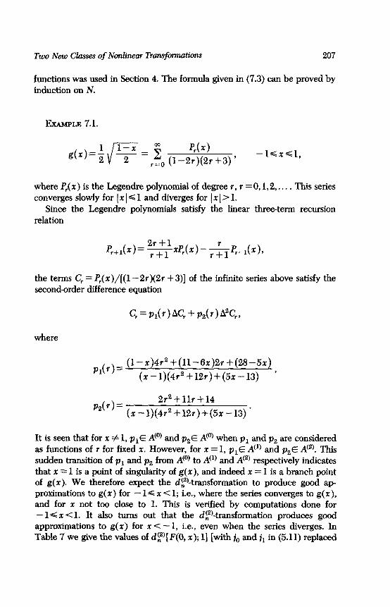
It is seen that for x # 1, pi E AC’) and paE A(o, when p, and p, are considered as functions of r for fixed X. However, for x = 1, p,~ A(‘) and p,E A”). This sudden transition of pr and p, from A(‘) to A(‘) and Ac2) respectively indicates that x = 1 is a point of singularity of g(x), and indeed x = 1 is a branch point of g(x). We therefore expect the d~kansformation to produce good ap- proximations to g(x) for - 1~ x < 1; i.e., where the series converges to g(x), and for x not too close to 1. This is verified by computations done for - 19 x <l. It also turns out that the dr)-transformation produces good approximations to g(x) for x < - 1, i.e., even when the series diverges. In Table 7 we give the values of dF)[F(O, x); l] [with j. and jr in (5.11) replaced
208 DAVID LEVIN AND AVBAM SIDI
TABLE 7 VALUES OF THE APPROXIMATIONS
dc,“[ F(0, x); l] TO g(x) = d-/2’
n dc2’[ F(0 9 - 1.5); l] ” rft2’[ F(0 ,. 0 5). , I] n d”[ F(0 ,* 0 9). 3 n I]
2 0.559015 0.2505 0.116 4 0.559016998 0.249998 0.1114 6 05590109943 72 0.24999989 0.11177 8 0.55901699437493 0.24999 99997 8 0.111800 10 0.55901099437485 0.25000OOOOO27 0.1118039
Exact 0.5599169943 74947 o.25OOOOOOOOOO 0.111803398874
“For x = - 1.5,0.5,0.9, and n = 2(2)10. Exact values of g(z) are given in the Bottom row.
by their upper bound, which is zero] for x = - 1.5,0.5,0.9, where F(& x) is
the $th partial sum of the infinite series evaluated at x; i.e., F(& x) = Z;:;P,(x)/[(l-2r)(2r +3)], and F(0, x) = 0.
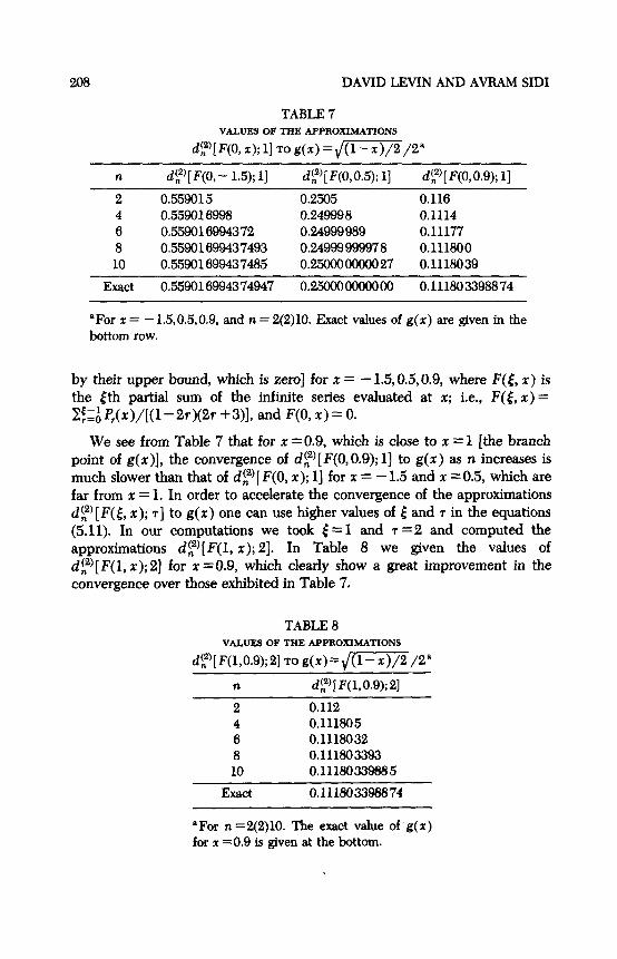
We see from Table 7 that for x ~0.9, which is close to x = 1 [the branch point of g(x)], the convergence of d,“)[ F(0,O.Q); l] to g(x) as n increases is much slower than that of df)[ F(0, x); l] for x = - 1.5 and x ~0.5, which are far from x = 1. In order to accelerate the convergence of the approximations d:) [ F(& x); T] to g(x) one can use higher values of [ and 7 in the equations (5.11). In our computations we took 4 = 1 and T =2 and computed the approximations d$)[F(l, x); 21. In Table 8 we given the values of dF)[ F(l, x);2] for x =O.Q, which clearly show a great improvement in the convergence over those exhibited in Table 7.
TABLE 8 VALUES OF THE AFPROXIMATIONS
@‘[F(1,0.9);2] TO g(r)=dw/2a
n dF’[F(l,0.9);2]
2 0.112 4 0.111805 6 0.1118032 8 0.111803393 10 0.11180339885
Exact 0.111803398874
*For n==2(2)10. The exact value of’g(x) for x =0.9 is given at the Bottom.
Two New Classes of Nonlinear Tramfmtkms 209
EXAMPLE 7.2.
g(x)=sgnr = ; s shgy-ll)x, --a-=X-CT.
r=l
The terms f(r) = sin(2r -1)x, r = 1,2,. . . , satisfy the three-term recursion relation
f(r+1)=2cos2xf(r)-f(r-1);
hence the terms C, = [4sin(2r - 1)x1/[ n(2r - 1)] of the infinite series satisfy the secondorder difference equation
c, = P~(WG + p,(r)A2C,,
where
P,(r)= -1+ (l_~f;223;);2;+l) ’
p2(r) = - (1 -co~.&~~4r +2) *
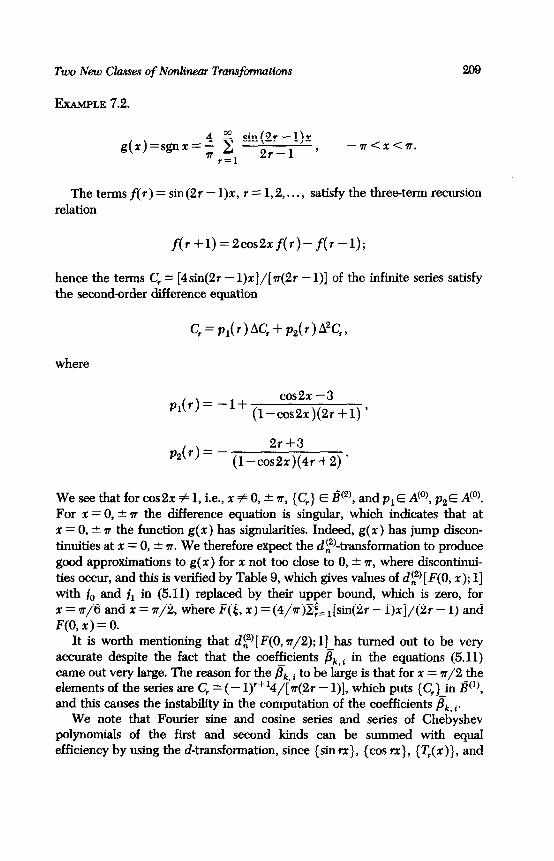
We see that for cos2x # 1, i.e., x # 0, * 7r, {C,} E B(‘), and p,~ A(‘), p,~ A(‘). For r = 0, k s the difference equation is singular, which indicates that at x = 0, k s the function g(x) has signularities. Indeed, g(x) has jump discon- tinuities at x = 0, 2 7r. We therefore expect the d~%ransformation to produce good approximations to g(x) for x not too close to 0, * 7~, where discontinui- ties occur, and this is verified by Table 9, which gives values of d,“,[ F(0, x); l] with i. and ji in (5.11) replaced by their upper bound, which is zero, for r = 7r/6 and x = r/2, where F(& x) =(4/s)&[sin(2r - l)r]/(2r - 1) and F(O,x)=O.
It is worth mentioning that dF)[F(O, r/2); l]_has turned out to be very accurate despite the fact that the coefficients Pk,< in the equations (5.11) came out very large. The reason for the &, i to be large is that for x = 7r/2 the elements of the series are C, = (- 1)‘+‘4/[ lr(2r - l)], which puts {C,.} in B(l), and this causes the instability in the computation of the coefficients &, i.
We note that Fourier sine and cosine series and series of Chebyshev polynomials of the first and second hinds can be summed with equal efficiency by using the d-transformation, since {sin 1x}, {cos rx}, {T,(z)}, and
210 DAVID LJWIN AND AVRAM SIDI
TABLE 9 VALUES OF THE APPROXIMATIONS
d’,2’[ F(0, r); l] TO g(x) = sgn xa
n d2’[ F(0, n/6); l] n @[ F(0, n/2); 11
2 1.032 1.00010 4 1.OcQ31 0.99999 983 6 0.99997 9 1.OOOOOOO36 8 0.999999908 0.999999999980 10 0.99999999932 0.99999999999993
‘For x = n/6 and I = a/2, and n = 2(2)10.
{t&(x)}, where T,(x) and U,(x) are the Chebyshev polynomials of the first and second kinds respectively, all satisfy similar recursion relations, namely,
sin(r+l)x=2cosxsinrx-sin(r-1)x,
cos(r+l)x=2cosxcos?x-cos(7-I)X,
T,+,(x)=2xT,(x)- T,-,(x)*
u,+,(x)=2xu,(+ v,-,(x)9
for r&l.
EXAMPLE 7.3.
g(x)=logi =2 f J&x> r=l [X,J,(A,)]2 ’ OCxG1,
where A, is the rth positive zero of JO(x). We have not been able to find a recursion relation that the terms
c,=Zr,(h,~)/[X,J,(h,)]~ of this infinite series satisfy; however, we can prove that {C,} E B -c2). For this we shall make use of the following results [16]:
X,=(r-$)a+a(r),
Hjl)(x)= e i(x-vn/2-n/4)by(;r),
(7.4)
(7.5)
J,(x)=ReHi’)(x), (7.6)
Two New Classes of Nonlinear Transfmtim 211
where u(r), considered as a function of r, is in A’-“; b,(x), considered as a function of x is in A(-1/2)* 9 > and Hi’)(x) is the Hankel function of the first kind of order v.
First of ah, we see from (7.4) that l/X: considered as a function of r is in AcP2). Secondly, from (7.5) and (7.6)
J,(x,)=ReHI’)(X,)=Re{e +=+=W+7 - 7r/4+ u(r)]}
=(-1)“‘Re{ein(r)bl[rrr-lr/4+a(r)]}.
Now since a E A’-‘), i.e., u(r) = O(r-‘) as r + cc, we have eiacr)E A(‘). Using the fact that b,[r~ - 7r/4+ a(r)] E A(-li2) [since b,(r)~ A’-1/2)], we have that .I1( A,) E A(-‘/2) and hence 1/[J1(h,)]2~ A(‘).
Finally, we show hat {.Io(h,~)} for fix e d x is in Bc2), Using (7.4) and (7.5), we have
Z-@(A,x) = eirlrrK(r),
where K( r ) = eiacr)’ e A(‘) and b [nr*-n!,;+u(r)x]~A-
i(‘“‘/4~~~4~bo~m~,; nx/4 + u(r)x]}. Since eiocr)‘E
-Ys we have K(r) E A(-1/2). Since
{eir”‘} E B for x fixed, we have {iY~l)(&)} E B(‘) using CoroIIary 3 to Lemma 3. Also since J,(A,x) = [H$‘)(h,x)+ @)(X,x)]/2, we have {I,( h,, x)} E B(‘) in accordance with CorolIary 2 of Lemma 3. And finahy
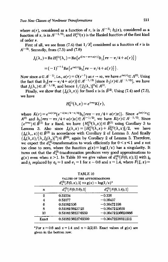
{Jo(~,~)/[~,J1(~,)12] E @2), again by Corollary 2 of Lemma 3. Therefore, we expect the d, (2)-transformation to work efficiently for 0 < x G 1 and x not too close to zero, where the function g(x) = log(l/x) has a singularity. It turns out that the @-transformation produces very good approximations to g(x) even when x > 1. In Table 10 we give values of dF)[ F(0, x); l] with to and jl replaced by a0 = 1 and u1 = 1 for x = 0.6 and x = 1.4, where F([, x) =
TABLE 10 VALUES OF THE APPROXIMATIONS
d”‘[ F(0, x); 11 TO g(x) = log(+)” ”
n c.P’[ F(O,0.6); l] n dC2’[ F(0 14). l] n 9.1
2 0.51034 -0.336 4 0.51077 -0.36437 6 0.51082 556 - 0.36472 198 8 0.51082 56237 25 -0.3647223659 10 0.51082 56237 6559 -0.36472236620986
Exact 0.51082 56237 65599 -0.36472236621212
aFor 2 = 0.6 and x = 1.4 and n = 2(2)10. Exact values of g(r) are given in the bottom row.
212 DAVID LEYIN AND AVRAM SIDI
El Mw/[~,Jl(~,)12 and F(0, x) = 0. Numerical results indicate that i0 = ii = 0.
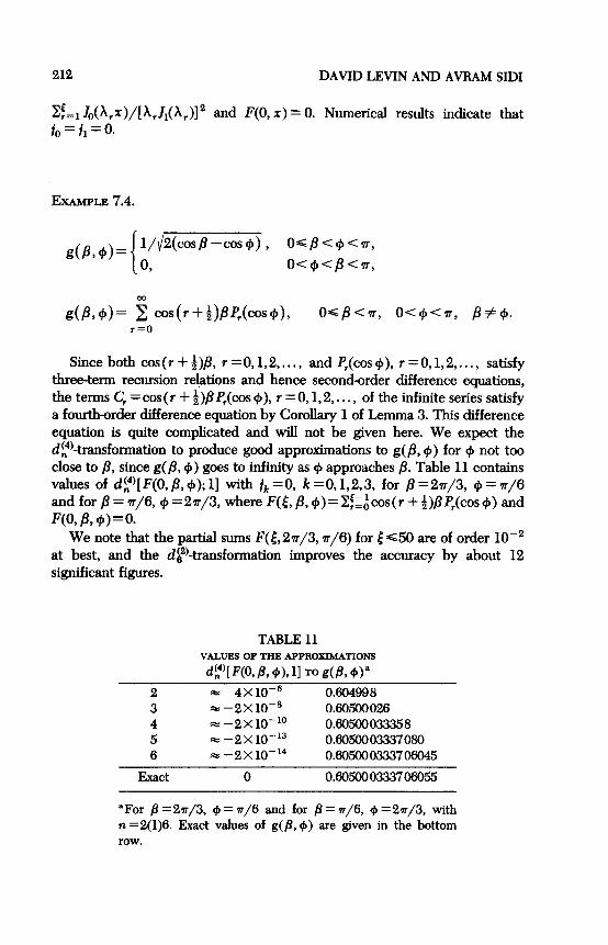
dPd4= o r 1/\/2(cos/3-cos+), OGp<c#s<Tr,
, oc+</3<n,
Since both cos(r + ;)a, r =O, 1,2,. . . , and P,(cos +), r =O, 1,2,. . . , satisfy three-term recursion relations and hence second-order difference equations, the terms C, = cos (r + 8)/3 P,(cos t$), r =O, 1,2,. . . , of the infinite series satisfy a fourth-order difference equation by Corollary 1 of Lemma 3. This difference equation is quite complicated and will not be given here. We expect the dr)-transformation to produce good approximations to g(/3, +) for $8 not too close to j3, since g(& +) goes to infinity as + approaches /3. Table 11 contains values of dff)[F(O, j?, +); l] with ik =O, k =O, 1,2,3, for /? =2~r/3, + = rr/6 and for /3 = r/6, + =2~/3, where F(& 8, +)=ZfiAcos(r + f)PP,(cos +) and F(0, 8, cp)=O.
We note that the partial sums F([,2~/3,7r/6) for 4 G50 are of order 10m2 at best, and the d&2kansformation improves the accuracy by about 12 significant figures.
2 3 4 5 6
Exact
TABLE 11 VALUES OF THE APPROXIMATIONS
&4’[F@, I% +X 11 TO d/% $1”
= 4x10-e 0.604998 E+r -2x10⁻⁸ 0.60500026 W -2x10-‘0 0.60500033358 a-gx10-‘3 0.6050003337080 s=a-2x10-14 0.605000333706045
0 0.605000333706055
“For j3 =2~/3, $ = r/6 and for j3 = 97/S, + =2~/3, with n =2(l)& hct values of g(B, up) are given in the bottom row.
Two New Clusses of Nonlinear Trarwfmtbns 213
8. COMPUTATIONAL ASPECTS
In this section we shall describe briefly the computational aspects of the D-transformation, those of the d-transformation being similar.
When one is given a function f to integrate between zero and infinity, one should find out whether this function is in B(“) for some m and what this m is. Then, as was described in Section 4, the parameters jk in (2.24) should be replaced either by their upper bounds or by the ok whose determination was also described in Section 4. Once this is done, one should pick up the xI in (2.24) in such a way that the function f(t) has a smooth behavior between two consecutive x1’s and hence can be integrated accurately there without much effort being wasted. An example of poor behavior was given in Example 4.3, where f(t) = sin(at’ + bt) with a = 7r/2, b = 0 and with a = 7r/2, b = 7r/2. This function oscillates with increasing frequency as t becomes large, and if the distance between xt and xl+i is so large as to enable the function to oscillate a large number of times there, then the accurate computation of the integrals uI = Q_ 1 f(t) dt and h ence of F(xf) = Xi=, u, becomes a hard task. This is the reason why we took x, = E + (j - 1)r with 6 and r small (actually we took 4 = 0.2 and r = 0.2). With this choice of 6 and r, at least the first few u, which are needed for the computation of Dis)[F(t); r], say up to n = 15, can be computed accurately without any difficulty. We have already pointed out in Example 4.4 that sometimes the choice X~ = 6 + (i - 1)~ causes the approximations DA”)[F([); r] to be poor even for large n, and this problem can be dealt with by taking, for example, x1 = [ +(i - l)%, I > 1, or xI = [e(‘-‘)‘; in Example 4.4 we chose the latter. Now that we have chosen the xt appropriately, we compute the t.+, the F(x,), and the matrix of the equations (2.24) and solve the linear system in (2.24). We used the LINSYST subroutine subprogram [18] to solve the linear system in (2.24). This subroutine solves linear systems by LU decomposition and iterative improvement. The use of Cramer’s rule, as in (2.25) for example, is not advised, since as n and hence the number of equations become large, the determinant of the linear system (2.24) decreases rapidly and thus errors are introduced in the computation of the approximations 0:“). Also it is worth mentioning that the system (2.24) becomes very ill conditioned as n increases. However, this does not seem to affect the approximations DA”).
In order to give proper meaning to the numerical results, attention must be paid to the coefficients &, *, as well as 0;“). in the solution of (2.24). In most cases the D-transformation produces approximations DA”) which, as n be- comes large, converge very quickly to the right value. For instance, in most of the examples in Section 4, 0:“) is correct to ten significant figures or more. As the D,$“), n=1,2 ,..., converge, the first few &(, for each k, approach the corresponding Bk,, in the asymptotic expansion in (2.23), and this can be recognized very easily even for small n.

214 DAVID LEVIN AND AVRAM SIDI
It may happen, though very rarely, that the convergence pattern of the approximations 0;“) is disrupted by some DA”‘), say for n = r; i.e., it may happen that D>“) is a worse approximation than D,?“], D$!‘] being better than D!_“1’. Thi. is accomp anied by a disruption in the convergence pattern of tbe first few Pk, i for each k to &( in (2X$), the rest of the coefficients becoming much larger than those for n = r f 1. The reason for this is that the matrix of the equations (2.24) for n = r, for computational purposes, is singular. Need- less to say, D,?“‘) should be discarded.
The authors are grateful to Profess0 I. M. Longmun for continuous support and encouragement of this work. The computations for this paper were carried out on the CDC 6600 computer at the Tel-Aviv University Computation center.
REFERENCES
1 H. L. Gray, T. A. Atchison, and G. V. McWilliams, Higher order G-transforma- tions, SZAM J. Numer. Anal. 8:365-381 (1971).
2 W. R. Schucany, H. L. Gray, and D. B. Owen, On bias reduction in estimation, J. Amer. Statist. Assoc. 66:524-533 (1971).
3 P. Wynn, On a device for computing the e,,,(S,) transformation, MTAC 10:91-96 (1956).
4 P. Wynn, Upon a second confluent form of the c-algorithm, Proc. Glasgow Math. Assoc. 5160-165 (1962).
5 D. L&n, Development of non-linear transformations for improving convergence of sequences, Znterttut. J. Cumput. Math. B3:371-388 (1973).
6 D. Levin, Ph.D. Thesis, Tel-Aviv Univ., 1975 (in Hebrew). 7 D. Levin, Numerical inversion of the Laplace transform by accelerating the
convergence of Bromwich’s integral, J. Cmnput. Appl. Math., 1:247-250 (1975). 8 D. Shanks, Non-linear transformations of divergent and slowly convergent se-
quences, J. Math. Phys. 34:1X? (1955). 9 I. M. Longman, A short table of j~l,,(t)t-“dt and j,“]l(t)t-“dt, MTAC
13:306-311 (1959). 10 I. M. Longman, On the generation of rational function approximations to Laplace
transform inversion with an application of viscoelastivity, SIAM Z. Appl. Math. 24:429-440 (1973).
11 H. J. Maehley, Rational approximations for transcendental functions, in Proceed- ings of the International Confmence on lnfonnation Processing, UNESCO, Butterworths, London, 1960.
12. J. T. Holdeman, Jr., A method for the approximation of functions defined by formal series expansions in orthogonal polynomials, Math. Comp. 23:275-287 (1969).
13 J. Fleischer, Non-linear Padi! approximauts for Legendre series, Z. Math. Phys. 14:246-248 (1973).
Two New Classes of Nonlinear Transfmtiom 215
14 C. W. Clenshaw and K. Lord, Rational approximations from Chebyshev series, in Studies in Numerical Analysis, Academic, London, 1974, pp. 95-113.
15 A. Sidi, Computation of the Chebyshev-Pad6 table, I. Cornput. Appl. Math. 1:69-71 (1975).
16 M. Abramowitz and I. A. Stegun, Handbook of Mathematical Functions with Formulas, Graphs, and Mathematical Tables, Dover, New York, 1968.
17 K. Knopp, Theory and Application of Znfinite Series, 2nd English ed. (transl. from the 4th German ed.), Blackie, Glasgow, 1951.
18 F4 UTF,X LINSYST, Univ. of Texas Computation Center, May 1988.
Note Added in Proof
The convergence analysis of the D- and d-transformations has been taken up by the second author within a more general framework in the paper
A. Sidi, Some properties of a generalization of the Richardson extrapolation process, J. Inst. Maths. Applies. 24:327-346 (1979).
In this paper the question of the significance of the xl that go into the definition of the D-transformation is also considered.
It turns out that by selecting the xl in an appropriate manner, the Dtransformation can be modified and made more efficient for integrands f(x) that oscillate an infinite number of times as x --) co. This subject is taken up in the papers
A. Sidi, Extrapolation methods for oscillatory infinite integrals, J. Inst. Maths. Applies. 2&l-20 (1986).
A. Sidi, The numerical evaluation of very oscillatory infinite integrals by extrapolation, Math. Camp. 38 (1982) (in press).
Convergence properties of the T-transformation of Levin [5] have been taken up in the papers
A. Sidi, Convergence properties of some non-linear sequence transforma- tions, Math. Comp. 33:315-326 (1979).
A. Sidi, Analysis of convergence of the T-transformation for power series, Math. Camp. 35:833-850 (1986).
The t- and u-transformations, which are special cases of the T-transformation, are simply d(l)-transformations as mentioned in Section 6 of the present work.

![STOCHASTIC HEAT EQUATION WITH INFINITE - LSUMath175].pdf · STOCHASTIC HEAT EQUATION WITH INFINITE DIMENSIONAL FRACTIONAL NOISE: L2-THEORY ... integrals are of Hitsuda-Skorohod type](https://img.pdfslide.net/doc/110x75/5b146a867f8b9a3e7c8cd6ea/stochastic-heat-equation-with-infinite-lsumath-175pdf-stochastic-heat-equation.jpg)