Embed Size (px)
Citation preview
Physica D 199 (2004) 201–222
Two-phase resonant patterns in forced oscillatory systems:boundaries, mechanisms and forms
Arik Yochelisa,∗, Christian Elphickb, Aric Hagbergc, Ehud Merona,d
a Department of Physics, Ben-Gurion University, Beer Sheva 84105, Israelb Centro de Fisica No Lineal y Sistemas Complejos de Santiago, Casilla 17122, Santiago, Chile
c Mathematical Modeling and Analysis, Theoretical Division, Los Alamos National Laboratory, Los Alamos, NM 87545, USAd Department of Solar Energy and Environmental Physics, BIDR, Ben Gurion University, Sede Boker Campus 84990, Israel
Abstract
We use the forced complex Ginzburg–Landau (CGL) equation to study resonance in oscillatory systems periodically forcedat approximately twice the natural oscillation frequency. The CGL equation has both resonant spatially uniform solutions andresonant two-phase standing-wave pattern solutions such as stripes or labyrinths. The spatially uniform solutions form a tongue-shaped region in the parameter plane of the forcing amplitude and frequency. But the parameter range of resonant standing-wavepatterns does not coincide with the tongue of spatially uniform oscillations. On one side of the tongue the boundary of resonantpatterns is inside the tongue and is formed by the nonequilibrium Ising Bloch bifurcation and the instability to traveling waves. Onthe other side of the tongue the resonant patterns extend outside the tongue forming a parameter region in which standing-wavep e inside thet r analysisn ns outsidet tion.©
K
1
oscillators aturalo in ratios
e
0d
atterns are resonant but uniform oscillations are not. The standing-wave patterns in that region appear similar to thosongue but the mechanism of their formation is different. The formation mechanism is studied using a weakly nonlineaear a Hopf–Turing bifurcation. The analysis also gives the existence and stability regions of the standing-wave patter
he resonant tongue. The analysis is supported by numerical solutions of the forced complex Ginzburg–Landau equa2004 Elsevier B.V. All rights reserved.
eywords:Resonant pattern; Forced oscillatory system; Ginzburg–Landau equation
. Introduction
Resonance phenomena in forced oscillatory systems have mostly been studied in the context of a singleuch as the pendulum[1–3]. The resonant behavior is manifested by the ability of the system to adjust its nscillation frequency to a rational fraction of the forcing frequency. Thus, the system may respond, or lock,
∗ Corresponding author.E-mail addresses:[email protected] (A. Yochelis); [email protected] (C. Elphick); [email protected] (A. Hagberg);
[email protected] (E. Meron)
167-2789/$ – see front matter © 2004 Elsevier B.V. All rights reserved.oi:10.1016/j.physd.2004.08.015
202 A. Yochelis et al. / Physica D 199 (2004) 201–222
1/n (n = 1,2,3, . . .) of the forcing frequency and at additional fractions determined by the Farey hierarchy[4]. Thenatural frequency range, where the system locks to the forcing frequency, increases with the forcing amplitude andforms a tongue-shaped region (Arnol’d tongues) in the amplitude–frequency plane. The parameter region pertainingto oscillations at 1/n the forcing frequency is occasionally referred to as then: 1 resonance tongue.
More recently resonance phenomena have been studied in spatially extended systems using uniform time periodicforcing [5–21]. These systems demonstrate another property of resonance phenomena; although any spatial pointin the system oscillates at the same fraction 1/n of the forcing frequency, the phase of oscillation may assumeone ofn different values and may vary from one spatial domain to another[8,22]. In the 2:1 resonance, there aretwo stable phases of oscillations (differing from one another byπ) and fronts that shift the oscillation phase byπ may appear. In the 4:1 resonance, there are four stable phases and two types of fronts may appear; fronts canshift the oscillation phases by eitherπ or π/2. Along with these fronts spatial patterns, such as spiral waves andstanding-wave labyrinths, may appear[10,12,20].
In this paper, we study to the 2:1 resonance case and the conditions for resonant behavior in spatially extendedsystems as compared with those of a single oscillator. The study is based on a variant of the complex Ginzburg–Landau (CGL) equation which describes the dynamics of the oscillation amplitude near the Hopf bifurcation. Amongour findings are non-resonant patterns in a range of resonant uniform oscillations and resonant patterns in a rangewhere uniform oscillations are not resonant. The results derived in this paper extend the analytical and numericalresults presented in Ref.[20].
The paper is organized as follows. InSection 2, we derive the boundaries of the 2:1 resonance tongue for uniformoscillations. This is the domain where the system is bistable and front solutions may exist. InSection 3, we study twofront instabilities and the patterns that arise from them. The results are used to determine the range where resonantpatterns appear inside the 2:1 resonant tongue of uniform oscillations. InSection 4, we determine the conditions forthe prevalence of resonant standing wavesoutsidethe resonance tongue and show that the formation mechanismdiffers from that of standing waves inside the tongue. We conclude with a summary and a discussion of the resultsin Section 5.
2. The 2:1 resonance tongue
i thes
wa s. Thea CGLe
I sd lL dicf eo
Consider an extended system undergoing a Hopf bifurcation to uniform oscillations at a frequencyΩ. The systems now uniformly forced at a frequencyωf ≈ 2Ω. Near the Hopf bifurcation a typical dynamical variable ofystem can be written as
u = u0 + [Aeiωt + c.c.] + · · · , (1)
hereu0 is the value ofu when the system is at the rest state undergoing the Hopf bifurcation,A is a complexmplitude,ω := ωf /2, c.c. stands for the complex conjugate, and the ellipses denote higher order termmplitude of oscillationA is slowly varying in space and time and for weak forcing is described by the forcedquation[23–26]
∂tA = (µ+ iν)A+ (1 + iα)∇2A− (1 + iβ)|A|2A+ γA∗. (2)
n this equation,µ represents the distance from the Hopf bifurcation,ν = Ω− ωf /2 the detuning,α representispersion,β represents nonlinear frequency correction,γ the forcing amplitude, and∇2 is the two-dimensionaaplacian operator. The termA∗ is the complex conjugate ofA and describes the effect of the weak perio
orcing[23]. Throughout this paper, we will mostly be concerned withEq. (2) for the amplitude of oscillations. Thscillating system inEq. (1) will be referred to as the “original system.”
A. Yochelis et al. / Physica D 199 (2004) 201–222 203
To find the resonance boundary of uniform oscillations, we writeA = R exp(iφ) and consider uniform solutionsof Eq. (2). The amplitudeR and the phaseφ obey the equations:
R = µR−R3 + γR cos 2φ, (3a)
φ = νR− βR3 − γR sin 2φ. (3b)
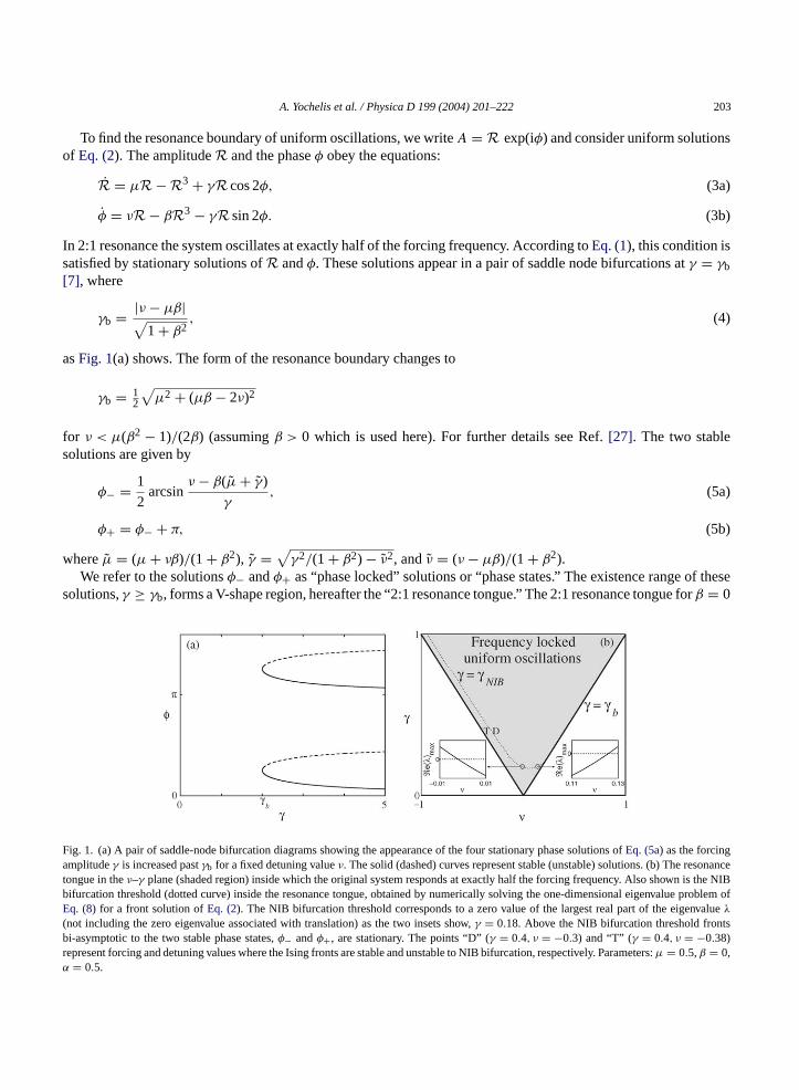
In 2:1 resonance the system oscillates at exactly half of the forcing frequency. According toEq. (1), this condition issatisfied by stationary solutions ofR andφ. These solutions appear in a pair of saddle node bifurcations atγ = γb[7], where
γb = |ν − µβ|√1 + β2
, (4)
asFig. 1(a) shows. The form of the resonance boundary changes to
γb = 12
√µ2 + (µβ − 2ν)2
for ν < µ(β2 − 1)/(2β) (assumingβ > 0 which is used here). For further details see Ref.[27]. The two stablesolutions are given by
φ− = 1
2arcsin
ν − β(µ+ γ)
γ, (5a)
φ+ = φ− + π, (5b)
whereµ = (µ+ νβ)/(1 + β2), γ =√γ2/(1 + β2) − ν2, andν = (ν − µβ)/(1 + β2).
We refer to the solutionsφ− andφ+ as “phase locked” solutions or “phase states.” The existence range of thesesolutions,γ ≥ γb, forms a V-shape region, hereafter the “2:1 resonance tongue.” The 2:1 resonance tongue forβ = 0
Fa onancet s the NIBb problem ofE value( tsbrα
ig. 1. (a) A pair of saddle-node bifurcation diagrams showing the appearance of the four stationary phase solutions ofEq. (5a) as the forcingmplitudeγ is increased pastγb for a fixed detuning valueν. The solid (dashed) curves represent stable (unstable) solutions. (b) The res
ongue in theν–γ plane (shaded region) inside which the original system responds at exactly half the forcing frequency. Also shown iifurcation threshold (dotted curve) inside the resonance tongue, obtained by numerically solving the one-dimensional eigenvalueq. (8) for a front solution ofEq. (2). The NIB bifurcation threshold corresponds to a zero value of the largest real part of the eigenλ
not including the zero eigenvalue associated with translation) as the two insets show,γ = 0.18. Above the NIB bifurcation threshold froni-asymptotic to the two stable phase states,φ− andφ+, are stationary. The points “D” (γ = 0.4, ν = −0.3) and “T” (γ = 0.4, ν = −0.38)epresent forcing and detuning values where the Ising fronts are stable and unstable to NIB bifurcation, respectively. Parameters:µ = 0.5,β = 0,= 0.5.
204 A. Yochelis et al. / Physica D 199 (2004) 201–222
is shown inFig. 1(b). Forβ = 0 the tongue gets wider and is shifted to the right (β > 0) or to the left (β < 0).Outside the resonance tongue uniform solutions describe unlocked oscillations.
For the analysis that follows we rewriteEq. (2) in terms of the real and imaginary parts of the amplitude,U := ReA andV := ImA:(
∂tU
∂tV
)= (L−N )
(U
V
), (6)
whereL is the linear operator
L =[
(µ+ γ) + ∇2 −ν − α∇2
ν + α∇2 (µ− γ) + ∇2
],
andN includes the nonlinear terms
N = (U2 + V 2)
[1 −ββ 1
].
3. Spatial patterns inside the 2:1 resonance tongue
Inside the 2:1 resonance tongue the system is bistable and front solutions, bi-asymptotic to the two stable phasestates, exist. Patterns in bistable systems are strongly affected by two types of front instabilities[28,29]. The first isthe nonequilibrium Ising Bloch (NIB) bifurcation in which a stationary “Ising” front solution loses stability to a pairof counter-propagating “Bloch” front solutions. This instability designates a transition from stationary patterns totraveling waves. The second front instability is a transverse instability (occasionally also referred to as modulationalor morphological instability) where wiggles along the front line grow in time. A transverse front instability of anIsing front often leads to stationary labyrinthine patterns. In the context of forced oscillations the NIB bifurcationh ee nt patternsr
the 2:1r in a veryn rns repre-sf are stablet
3
b f theI
as been studied in Refs.[7,30–33]and the transverse instability in Ref.[17]. In the following we extend thesarlier works and use the results to delineate the range within the 2:1 resonance tongue where resonaeside.
Finite wavenumber instabilities of the uniform phase states may also lead to pattern formation insideesonance tongue. A linear stability analysis of the phase states indeed reveals such an instability butarrow range near the 2:1 resonance boundary. The instability leads to large amplitude stationary patteenting resonant oscillations of the original system. For further details the reader is referred to Ref.[27]. In theollowing analyzes performed inside the tongue we assume a parameter range for which the phase stateso nonuniform perturbations.
.1. The nonequilibrium Ising Bloch (NIB) bifurcation
In the case,α = β = 0, the NIB bifurcation occurs atγNIB =√ν2 + (µ/3)2 [32,33]. To evaluate the NIB
ifurcation across the resonance tongue for non-zeroα or β values we use a numerical eigenvalue analysis osing front solutionI (x). Inserting the form[
U(x, t)
V (x, t)
]= I (x) + e(x) eλt, (7)
A. Yochelis et al. / Physica D 199 (2004) 201–222 205
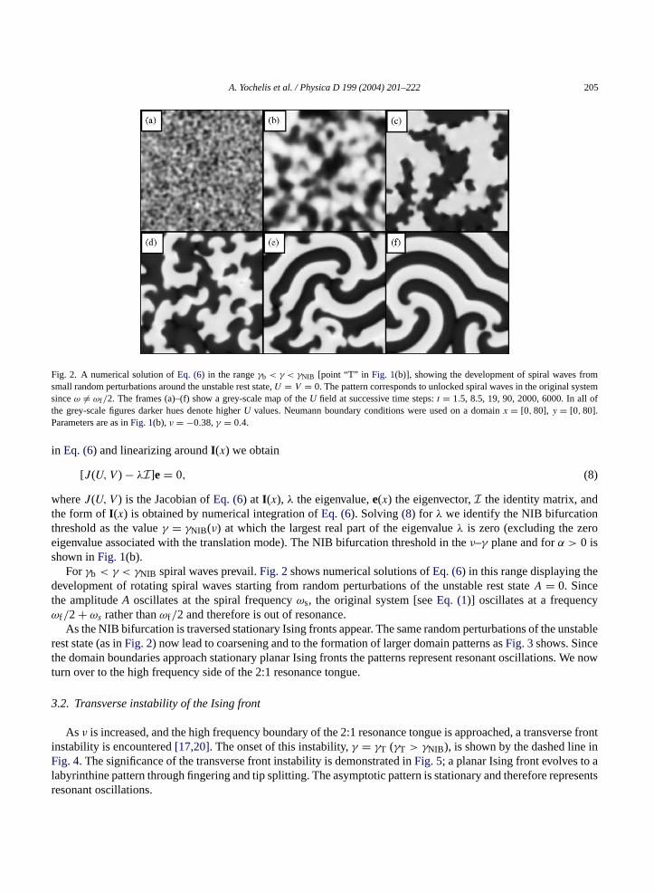
Fig. 2. A numerical solution ofEq. (6) in the rangeγb < γ < γNIB [point “T” in Fig. 1(b)], showing the development of spiral waves fromsmall random perturbations around the unstable rest state,U = V = 0. The pattern corresponds to unlocked spiral waves in the original systemsinceω = ωf /2. The frames (a)–(f) show a grey-scale map of theU field at successive time steps:t = 1.5, 8.5, 19, 90, 2000, 6000. In all ofthe grey-scale figures darker hues denote higherU values. Neumann boundary conditions were used on a domainx = [0,80], y = [0,80].Parameters are as inFig. 1(b), ν = −0.38,γ = 0.4.
in Eq. (6) and linearizing aroundI (x) we obtain
[J(U,V ) − λI]e= 0, (8)
whereJ(U,V ) is the Jacobian ofEq. (6) at I (x), λ the eigenvalue,e(x) the eigenvector,I the identity matrix, andthe form ofI (x) is obtained by numerical integration ofEq. (6). Solving(8) for λ we identify the NIB bifurcationthreshold as the valueγ = γNIB(ν) at which the largest real part of the eigenvalueλ is zero (excluding the zeroeigenvalue associated with the translation mode). The NIB bifurcation threshold in theν–γ plane and forα > 0 isshown inFig. 1(b).
Forγb < γ < γNIB spiral waves prevail.Fig. 2shows numerical solutions ofEq. (6) in this range displaying thedevelopment of rotating spiral waves starting from random perturbations of the unstable rest stateA = 0. Sincethe amplitudeA oscillates at the spiral frequencyωs, the original system [seeEq. (1)] oscillates at a frequencyωf /2 + ωs rather thanωf /2 and therefore is out of resonance.
As the NIB bifurcation is traversed stationary Ising fronts appear. The same random perturbations of the unstablerest state (as inFig. 2) now lead to coarsening and to the formation of larger domain patterns asFig. 3shows. Sincethe domain boundaries approach stationary planar Ising fronts the patterns represent resonant oscillations. We nowturn over to the high frequency side of the 2:1 resonance tongue.
3.2. Transverse instability of the Ising front
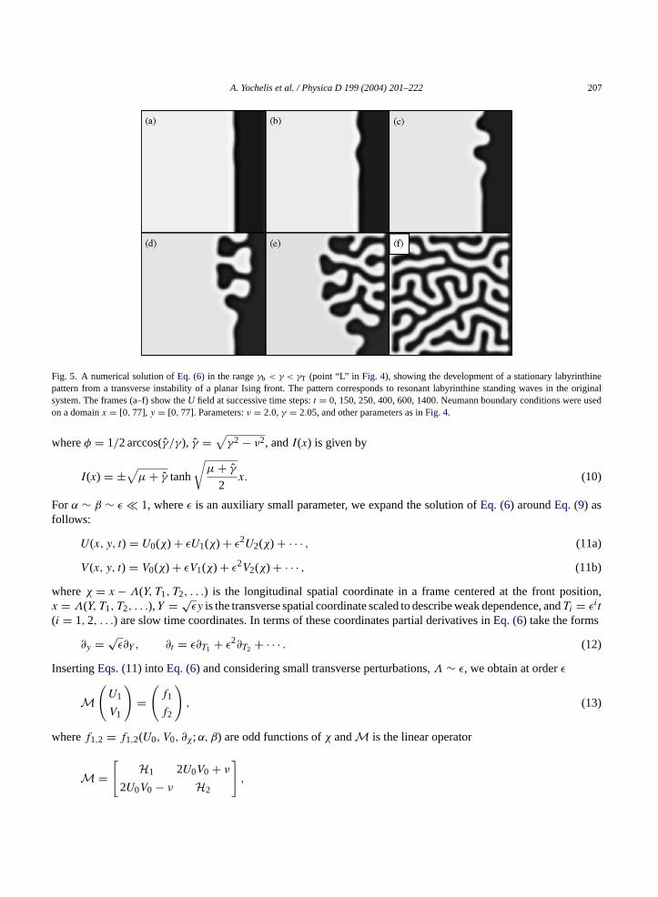
As ν is increased, and the high frequency boundary of the 2:1 resonance tongue is approached, a transverse frontinstability is encountered[17,20]. The onset of this instability,γ = γT (γT > γNIB), is shown by the dashed line inFig. 4. The significance of the transverse front instability is demonstrated inFig. 5; a planar Ising front evolves to alabyrinthine pattern through fingering and tip splitting. The asymptotic pattern is stationary and therefore representsresonant oscillations.

206 A. Yochelis et al. / Physica D 199 (2004) 201–222
Fig. 3. A numerical solution ofEq. (6) in the rangeγNIB < γ [point “D” in Fig. 1(b)] showing the coarsening of small domains into largerones separated by a planar Ising front. The asymptotic state is resonant since the Ising front is stationary and any point in the original system itoscillates at exactlyω = ωf /2. The frames (a)–(f) show theU field at successive time steps:t = 1.5, 8.5, 19, 90, 350, 850. Neumann boundaryconditions were used on a domainx = [0,80], y = [0,80]. Parameters are as inFig. 1(b), ν = −0.3, γ = 0.4.
We evaluated the transverse instability boundary by deriving a linear evolution equation for transverse frontmodulations as we now describe.Eq. (6), for α = β = 0 (but arbitraryν), has the exact Ising front solution
U0 = I(x) cosφ, (9a)
V0 = I(x) sinφ, (9b)
Fig. 4. The transverse instability line,γ = γT, for an Ising front inside the 2:1 resonance tongue. The dashed line denotes the approximateanalytical result ofγT given byEq. (24). The crosses (×) depict the conditionD = 0 whereD is calculated semi-analytically usingEq. (20),while the solid circles (•) represent results of a numerical two-dimensional eigenvalue analysis of the Ising front. Parameters:µ = 0.5,α = 0.35,β = 0.
A. Yochelis et al. / Physica D 199 (2004) 201–222 207
Fig. 5. A numerical solution ofEq. (6) in the rangeγb < γ < γT (point “L” in Fig. 4), showing the development of a stationary labyrinthinepattern from a transverse instability of a planar Ising front. The pattern corresponds to resonant labyrinthine standing waves in the originalsystem. The frames (a–f) show theU field at successive time steps:t = 0, 150, 250, 400, 600, 1400. Neumann boundary conditions were usedon a domainx = [0,77], y = [0,77]. Parameters:ν = 2.0, γ = 2.05, and other parameters as inFig. 4.
whereφ = 1/2 arccos(γ/γ), γ =√γ2 − ν2, andI(x) is given by
I(x) = ±√µ+ γ tanh
√µ+ γ
2x. (10)
Forα ∼ β ∼ ε 1, whereε is an auxiliary small parameter, we expand the solution ofEq. (6) aroundEq. (9) asfollows:
U(x, y, t) = U0(χ) + εU1(χ) + ε2U2(χ) + · · · , (11a)
V (x, y, t) = V0(χ) + εV1(χ) + ε2V2(χ) + · · · , (11b)
whereχ = x−Λ(Y, T1, T2, . . .) is the longitudinal spatial coordinate in a frame centered at the front position,x = Λ(Y, T1, T2, . . .),Y = √
εy is the transverse spatial coordinate scaled to describe weak dependence, andTi = εit
(i = 1,2, . . .) are slow time coordinates. In terms of these coordinates partial derivatives inEq. (6) take the forms
∂y = √ε∂Y , ∂t = ε∂T1 + ε2∂T2 + · · · . (12)
InsertingEqs. (11) into Eq. (6) and considering small transverse perturbations,Λ ∼ ε, we obtain at orderε
M
(U1
V1
)=(f1
f2
), (13)
wheref1,2 = f1,2(U0, V0, ∂χ;α, β) are odd functions ofχ andM is the linear operator
M =[
H1 2U0V0 + ν
2U0V0 − ν H2
],
208 A. Yochelis et al. / Physica D 199 (2004) 201–222
with
H1 = −(µ+ γ) − ∂2x + 3U2
0 + V 20 , H2 = −(µ− γ) − ∂2
x + 3V 20 + U2
0.
Solvability of Eq. (13) requires the right-hand side of this equation to be orthogonal to the null vectorΞ ofM†,the adjoint ofM. We evaluatedΞ numerically and found it to be an even function ofχ. Sincef1 andf2 are oddfunctions ofχ the solvability condition is automatically satisfied. For the same reasonU1 andV1 must be odd too(i.e. they preserve the symmetry of the zero-order approximation,U0, V0).
Proceeding to orderε2 we find
M
(U2
V2
)=[
(∂T1Λ− ∂2YΛ)U ′
0 + g1
(∂T1Λ− ∂2YΛ)V ′
0 + g2
], (14)
where the prime denotes derivation with respect to the argument and
g1,2 = g1,2(U0, V0, U1, V1, ∂χ;α, β)
are odd functions ofχ. Solvability ofEq. (14) leads to
∂T1Λ = ∂2YΛ. (15)
UsingEq. (15) into Eq. (14) we conclude thatU2 andV2 are again odd functions ofχ (i.e. preserve the symmetryof the lower order approximations).
Proceeding to orderε3 we find
M
(U3
V3
)=[∂T2ΛU
′0 + α(∂2
YΛ)V ′0 + (∂YΛ)2U ′′
0 + h1
∂T2ΛV′0 − α(∂2
YΛ)U ′0 + (∂YΛ)2V ′′
0 + h2
], (16)
where
a
w
a
w
T stable)w
h1,2 = h1,2(U0, V0, U1, V1, U2, V2, ∂χ;α, β)
re odd functions ofχ. Solvability ofEq. (16), yields
∂T2Λ = −αΣ∂2YΛ, (17)
here
Σ =∫∞−∞(Ξ1V
′0 −Ξ2U
′0) dχ∫∞
−∞(Ξ1U′0 +Ξ2V
′0) dχ
, (18)
ndΞ1 andΞ2 are the components of the null vectorΞ. InsertingEqs. (15) and (17) into Eq. (12), we obtain
∂tΛ = D∂2yΛ, (19)
here
D = 1 − αΣ. (20)
he sign ofD determines the stability of the Ising front to transverse perturbations; the front is stable (unhenD > 0 (D < 0) and the conditionD = 0 gives the instability thresholdγ = γT.
A. Yochelis et al. / Physica D 199 (2004) 201–222 209
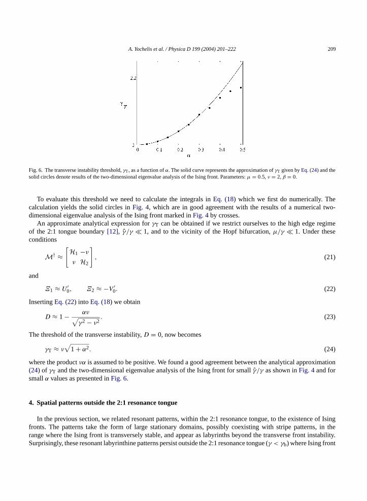
Fig. 6. The transverse instability threshold,γT, as a function ofα. The solid curve represents the approximation ofγT given byEq. (24) and thesolid circles denote results of the two-dimensional eigenvalue analysis of the Ising front. Parameters:µ = 0.5, ν = 2,β = 0.
To evaluate this threshold we need to calculate the integrals inEq. (18) which we first do numerically. Thecalculation yields the solid circles inFig. 4, which are in good agreement with the results of a numerical two-dimensional eigenvalue analysis of the Ising front marked inFig. 4by crosses.
An approximate analytical expression forγT can be obtained if we restrict ourselves to the high edge regimeof the 2:1 tongue boundary[12], γ/γ 1, and to the vicinity of the Hopf bifurcation,µ/γ 1. Under theseconditions
M† ≈[H1 −νν H2
], (21)
and
Ξ1 ≈ U ′0, Ξ2 ≈ −V ′
0. (22)
InsertingEq. (22) into Eq. (18) we obtain
D ≈ 1 − αν√γ2 − ν2
. (23)
The threshold of the transverse instability,D = 0, now becomes
γT ≈ ν√
1 + α2. (24)
where the productνα is assumed to be positive. We found a good agreement between the analytical approximation(24) of γT and the two-dimensional eigenvalue analysis of the Ising front for smallγ/γ as shown inFig. 4and forsmallα values as presented inFig. 6.
4. Spatial patterns outside the 2:1 resonance tongue
In the previous section, we related resonant patterns, within the 2:1 resonance tongue, to the existence of Isingfronts. The patterns take the form of large stationary domains, possibly coexisting with stripe patterns, in ther instability.S t
ange where the Ising front is transversely stable, and appear as labyrinths beyond the transverse fronturprisingly, these resonant labyrinthine patterns persist outside the 2:1 resonance tongue (γ < γb) where Ising fron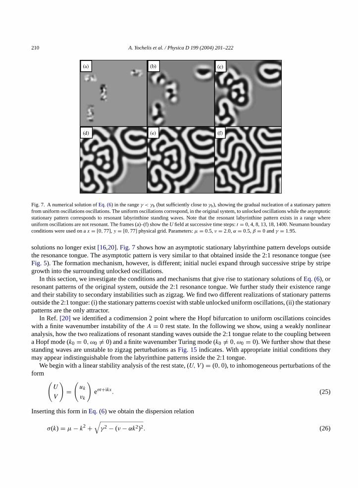
210 A. Yochelis et al. / Physica D 199 (2004) 201–222
Fig. 7. A numerical solution ofEq. (6) in the rangeγ < γb (but sufficiently close toγb), showing the gradual nucleation of a stationary patternfrom uniform oscillations oscillations. The uniform oscillations correspond, in the original system, to unlocked oscillations while the asymptoticstationary pattern corresponds to resonant labyrinthine standing waves. Note that the resonant labyrinthine pattern exists in a range whereuniform oscillations are not resonant. The frames (a)–(f) show theU field at successive time steps:t = 0, 4, 8, 13, 18, 1400. Neumann boundaryconditions were used on ax = [0,77], y = [0,77] physical grid. Parameters:µ = 0.5, ν = 2.0,α = 0.5,β = 0 andγ = 1.95.
solutions no longer exist[16,20]. Fig. 7shows how an asymptotic stationary labyrinthine pattern develops outsidethe resonance tongue. The asymptotic pattern is very similar to that obtained inside the 2:1 resonance tongue (seeFig. 5). The formation mechanism, however, is different; initial nuclei expand through successive stripe by stripegrowth into the surrounding unlocked oscillations.
In this section, we investigate the conditions and mechanisms that give rise to stationary solutions ofEq. (6), orresonant patterns of the original system, outside the 2:1 resonance tongue. We further study their existence rangeand their stability to secondary instabilities such as zigzag. We find two different realizations of stationary patternsoutside the 2:1 tongue: (i) the stationary patterns coexist with stable unlocked uniform oscillations, (ii) the stationarypatterns are the only attractor.
In Ref. [20] we identified a codimension 2 point where the Hopf bifurcation to uniform oscillations coincideswith a finite wavenumber instability of theA = 0 rest state. In the following we show, using a weakly nonlinearanalysis, how the two realizations of resonant standing waves outside the 2:1 tongue relate to the coupling betweena Hopf mode (k0 = 0, ω0 = 0) and a finite wavenumber Turing mode (k0 = 0, ω0 = 0). We further show that thesestanding waves are unstable to zigzag perturbations asFig. 15 indicates. With appropriate initial conditions theymay appear indistinguishable from the labyrinthine patterns inside the 2:1 tongue.
We begin with a linear stability analysis of the rest state, (U,V ) = (0,0), to inhomogeneous perturbations of theform (
U
V
)=(uk
vk
)eσt+ikx. (25)
Inserting this form inEq. (6) we obtain the dispersion relation
σ(k) = µ− k2 +√γ2 − (ν − αk2)2. (26)
A. Yochelis et al. / Physica D 199 (2004) 201–222 211
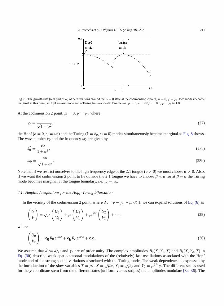
Fig. 8. The growth rate (real part ofσ) of perturbations around theA = 0 state at the codimension 2 point,µ = 0, γ = γc. Two modes becomemarginal at this point, a Hopf zero–kmode and a Turing finite–kmode. Parameters:µ = 0, ν = 2.0,α = 0.5, γ = γc ≈ 1.8.
At the codimension 2 point,µ = 0, γ = γc, where
γc = ν√1 + α2
, (27)
the Hopf (k = 0,ω = ω0) and the Turing (k = k0,ω = 0) modes simultaneously become marginal asFig. 8shows.The wavenumberk0 and the frequencyω0 are given by
k20 = να
1 + α2 , (28a)
ω0 = να√1 + α2
. (28b)
Note that if we restrict ourselves to the high frequency edge of the 2:1 tongue (ν > 0) we must chooseα > 0. Also,if we want the codimension 2 point to lie outside the 2:1 tongue we have to chooseβ < α for atβ = α the Turingmode becomes marginal at the tongue boundary, i.e.γc = γb.
4.1. Amplitude equations for the Hopf–Turing bifurcation
In the vicinity of the codimension 2 point, whered := γ − γc ∼ µ 1, we can expand solutions ofEq. (6) as(U
V
)= √
µ
(U0
V0
)+ µ
(U1
V1
)+ µ3/2
(U2
V2
)+ · · · , (29)
where(U0
V0
)= e0B0 eiω0t + ekBk eik0x + c.c.. (30)
We assume thatd := d/µ andγc are of order unity. The complex amplitudesB0(X, Y1, T ) andBk(X, Y2, T ) inEq. (30) describe weak spatiotemporal modulations of the (relatively) fast oscillations associated with the Hopfm ressed byt edf
ode and of the strong spatial variations associated with the Turing mode. The weak dependence is exphe introduction of the slow variablesT = µt, X = √
µx, Y1 = √µy andY2 = µ1/4y. The different scales us
or they coordinate stem from the different states (uniform versus stripes) the amplitudes modulate[34–36]. The
212 A. Yochelis et al. / Physica D 199 (2004) 201–222
eigenvectorse0 andek correspond to the eigenvaluesσ(0) andσ(k0), respectively, and are given by
e0 = 1 + iα
ρ
1
, ek =
(η
1
),
whereρ = √1 + α2 andη = α+ ρ.
Inserting the expansion(29) into Eq. (6) we obtain at orderµ
M
(U1
V1
)= −(2∂X∂x + ∂2
Y2)
(U0 − αV0
αU0 + V0
), (31)
where
M =[
−∂t + γc + ∂2x −ν − α∂2
x
ν + α∂2x −∂t − γc + ∂2
x
].
Defining an inner product as
〈f, g〉 := ω0k0
(2π)2
∫ ∫f ∗g dX dT, (32)
where the integrals are evaluated over the temporal oscillation period and over the stripe wavelength, the adjointoperator is
M† =[∂t + γc + ∂2
x ν + α∂2x
−ν − α∂2x ∂t − γc + ∂2
x
], (33)
a
T thise
w
nd its null vector is
1 =− (1 + iα)
ρ
1
e−iω0t +
(1
α− ρ
)e−ik0x. (34)
he solvability condition associated withEq. (31) is automatically satisfied and we can proceed to solvingquation. We find
(U1
V1
)= C
(U0
V0
)+ 0
ρ3
ν
DBk eik0x + c.c.
. (35)
hereD = 2ik0∂X + ∂2Y2
andC is an arbitrary constant which for simplicity, we set to zero.Proceeding to orderµ3/2 we obtain
M
(U2
V2
)= (N0 − L0)
(U0
V0
)− L1
(U1
V1
), (36)
A. Yochelis et al. / Physica D 199 (2004) 201–222 213
where
L0 =[
1 + d + ∂2X − ∂T −α∂2
X
α∂2X 1 − d + ∂2
X − ∂T
], N0 = (U2
0 + V 20 )
[1 −ββ 1
],
L1 = (2∂X∂x + ∂2Y2
)
[1 −αα 1
].
Solvability ofEq. (36) yields two coupled equations for the amplitudesB0 andBk:
∂TB0 =(
1 − i
αd
)B0 − (4 + im1)|B0|2B0 − (8ρη+ im2)|Bk|2B0 + (1 + iρ)(∂2
X + ∂2Y1
)B0, (37a)
∂TBk =(
1 + ρ
αd)Bk − 6ρη
(1 − β
α
)|Bk|2Bk − 4
(2 − 3
β
α
)|B0|2Bk − ρ2
2k20
(2ik0∂X + ∂2Y2
)2Bk, (37b)
where
m1 = 2(2ρ2 + 1)β
αρ, m2 = 4[2αρ(α+ 1) + (3ρ + α)]β
α− 4η.
Finally, by rescalingEqs. (37) back to the relatively fast space–time scales we obtain the following approximationto Eq. (6) in the vicinity of the codimension 2 point:(
U
V
)= e0A0 eiω0t + ekAk eik0x + c.c.+ · · · (38)
where the ellipses denote high order corrections and the amplitudesA0 andAk satisfy
∂tA0 =(µ− i
αd
)A0 − (4 + im1)|A0|2A0 − (8ρη+ im2)|Ak|2A0 + (1 + iρ)∇2A0, (39a)
4
sa
a
T eo thes
∂tAk =(µ+ ρ
αd)Ak − 6ρη
(1 − β
α
)|Ak|2Ak − 4
(2 − 3
β
α
)|A0|2Ak − ρ2
2k20
(2ik0∂x + ∂2y)
2Ak. (39b)
.2. Hopf and Turing pure-mode solutions
Eqs. (39) admit two families of pure-mode solutions and a mixed-mode solution[37,38]. The pure-mode solutionre
A0 = 12
√µ−K2 ei(Kx−ϑt)+iψ0, Ak = 0; (40a)
nd
A0 = 0, Ak =√αµ+ dρ − 2αρ2K2
6ρη(α− β)eiKx+iψk . (40b)
he phasesψ0 andψk are arbitrary constants which we set to zero andϑ = d/α+ µm1/4. In the context of thriginal system, the uniform-oscillation solution(40a) corresponds to unlocked uniform oscillations, whiletationary uniform solution(40b) represents resonant standing waves.
214 A. Yochelis et al. / Physica D 199 (2004) 201–222
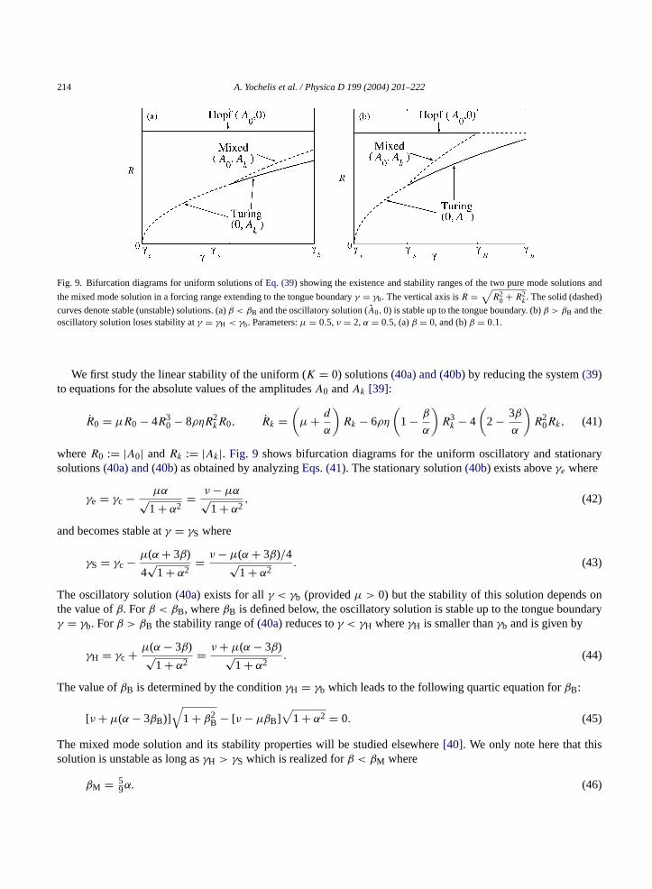
Fig. 9. Bifurcation diagrams for uniform solutions ofEq. (39) showing the existence and stability ranges of the two pure mode solutions and
the mixed mode solution in a forcing range extending to the tongue boundaryγ = γb. The vertical axis isR =√
R20 + R2
k. The solid (dashed)
curves denote stable (unstable) solutions. (a)β < βB and the oscillatory solution (A0,0) is stable up to the tongue boundary. (b)β > βB and theoscillatory solution loses stability atγ = γH < γb. Parameters:µ = 0.5, ν = 2,α = 0.5, (a)β = 0, and (b)β = 0.1.
We first study the linear stability of the uniform (K = 0) solutions(40a) and (40b) by reducing the system(39)to equations for the absolute values of the amplitudesA0 andAk [39]:
R0 = µR0 − 4R30 − 8ρηR2
kR0, Rk =(µ+ d
α
)Rk − 6ρη
(1 − β
α
)R3k − 4
(2 − 3β
α
)R2
0Rk, (41)
whereR0 := |A0| andRk := |Ak|. Fig. 9 shows bifurcation diagrams for the uniform oscillatory and stationarysolutions(40a) and (40b) as obtained by analyzingEqs. (41). The stationary solution(40b) exists aboveγe where
γe = γc − µα√1 + α2
= ν − µα√1 + α2
, (42)
and becomes stable atγ = γS where
γS = γc − µ(α+ 3β)
4√
1 + α2= ν − µ(α+ 3β)/4√
1 + α2. (43)
The oscillatory solution(40a) exists for allγ < γb (providedµ > 0) but the stability of this solution depends onthe value ofβ. Forβ < βB, whereβB is defined below, the oscillatory solution is stable up to the tongue boundaryγ = γb. Forβ > βB the stability range of(40a) reduces toγ < γH whereγH is smaller thanγb and is given by
γH = γc + µ(α− 3β)√1 + α2
= ν + µ(α− 3β)√1 + α2
. (44)
The value ofβB is determined by the conditionγH = γb which leads to the following quartic equation forβB:
[ν + µ(α− 3βB)]√
1 + β2B − [ν − µβB]
√1 + α2 = 0. (45)
The mixed mode solution and its stability properties will be studied elsewhere[40]. We only note here that thissolution is unstable as long asγH > γS which is realized forβ < βM where
βM = 59α. (46)
A. Yochelis et al. / Physica D 199 (2004) 201–222 215
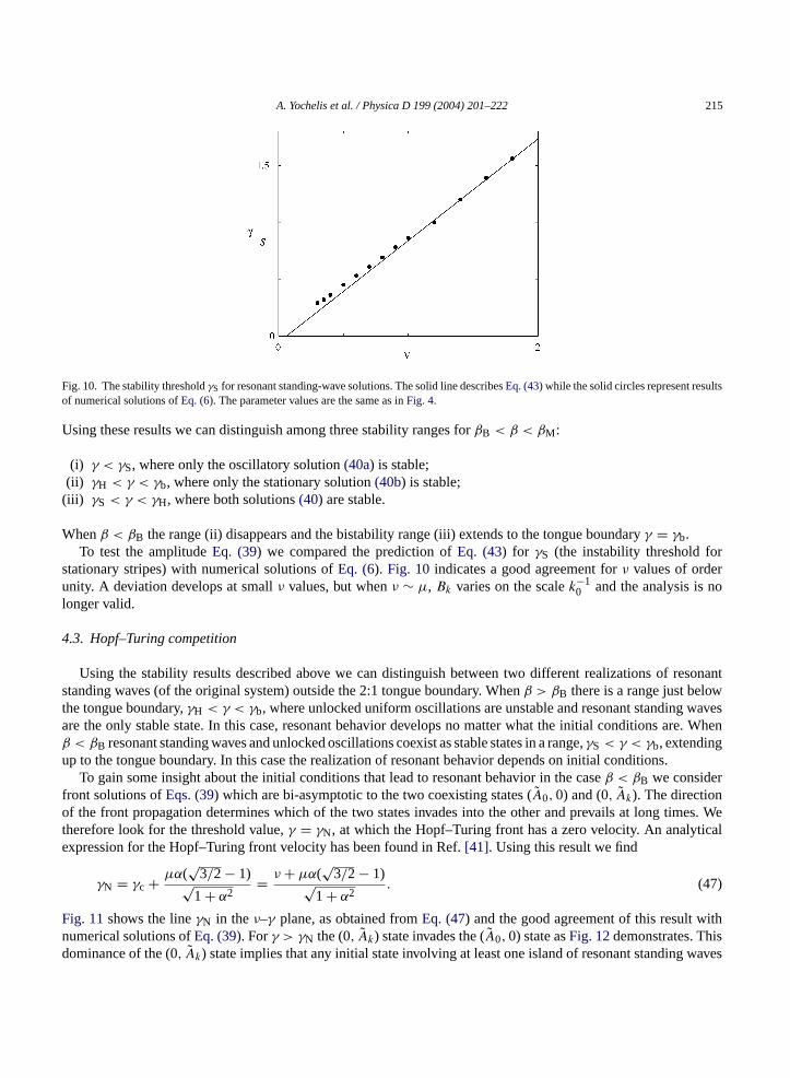
Fig. 10. The stability thresholdγS for resonant standing-wave solutions. The solid line describesEq. (43) while the solid circles represent resultsof numerical solutions ofEq. (6). The parameter values are the same as inFig. 4.
Using these results we can distinguish among three stability ranges forβB < β < βM:
(i) γ < γS, where only the oscillatory solution(40a) is stable;(ii) γH < γ < γb, where only the stationary solution(40b) is stable;
(iii) γS < γ < γH, where both solutions(40) are stable.
Whenβ < βB the range (ii) disappears and the bistability range (iii) extends to the tongue boundaryγ = γb.To test the amplitudeEq. (39) we compared the prediction ofEq. (43) for γS (the instability threshold for
stationary stripes) with numerical solutions ofEq. (6). Fig. 10 indicates a good agreement forν values of orderunity. A deviation develops at smallν values, but whenν ∼ µ, Bk varies on the scalek−1
0 and the analysis is nolonger valid.
4.3. Hopf–Turing competition
Using the stability results described above we can distinguish between two different realizations of resonantstanding waves (of the original system) outside the 2:1 tongue boundary. Whenβ > βB there is a range just belowthe tongue boundary,γH < γ < γb, where unlocked uniform oscillations are unstable and resonant standing wavesare the only stable state. In this case, resonant behavior develops no matter what the initial conditions are. Whenβ < βB resonant standing waves and unlocked oscillations coexist as stable states in a range,γS < γ < γb, extendingup to the tongue boundary. In this case the realization of resonant behavior depends on initial conditions.
To gain some insight about the initial conditions that lead to resonant behavior in the caseβ < βB we considerfront solutions ofEqs. (39) which are bi-asymptotic to the two coexisting states (A0,0) and (0, Ak). The directionof the front propagation determines which of the two states invades into the other and prevails at long times. Wetherefore look for the threshold value,γ = γN, at which the Hopf–Turing front has a zero velocity. An analyticalexpression for the Hopf–Turing front velocity has been found in Ref.[41]. Using this result we find
γN = γc + µα(√
3/2 − 1)√1 + α2
= ν + µα(√
3/2 − 1)√1 + α2
. (47)
Fig. 11shows the lineγN in theν–γ plane, as obtained fromEq. (47) and the good agreement of this result withnumerical solutions ofEq. (39). Forγ > γ the (0, A ) state invades the (A ,0) state asFig. 12demonstrates. Thisd waves
N k 0ominance of the (0, Ak) state implies that any initial state involving at least one island of resonant standing
216 A. Yochelis et al. / Physica D 199 (2004) 201–222
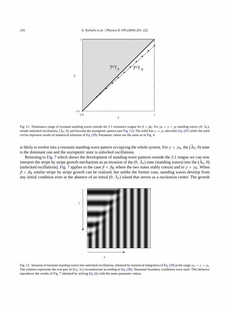
Fig. 11. Dominance range of resonant standing waves outside the 2:1 resonance tongue forβ < βB. ForγN < γ < γb standing waves, (0, Ak),invade unlocked oscillations, (A0,0), and become the asymptotic pattern (seeFig. 12). The solid lineγ = γN describesEq. (47) while the solidcircles represent results of numerical solutions ofEq. (39). Parameter values are the same as inFig. 4.
is likely to evolve into a resonant standing-wave pattern occupying the whole system. Forγ < γN, the (A0,0) stateis the dominant one and the asymptotic state is unlocked oscillations.
Returning toFig. 7which shows the development of standing-wave patterns outside the 2:1 tongue we can nowinterpret the stripe by stripe growth mechanism as an invasion of the (0, Ak) state (standing waves) into the (A0,0)(unlocked oscillations).Fig. 7applies to the caseβ < βB where the two states stably coexist and toγ > γN. Whenβ > βB similar stripe by stripe growth can be realized, but unlike the former case, standing waves develop fromany initial condition even in the absence of an initial (0, Ak) island that serves as a nucleation center. The growth
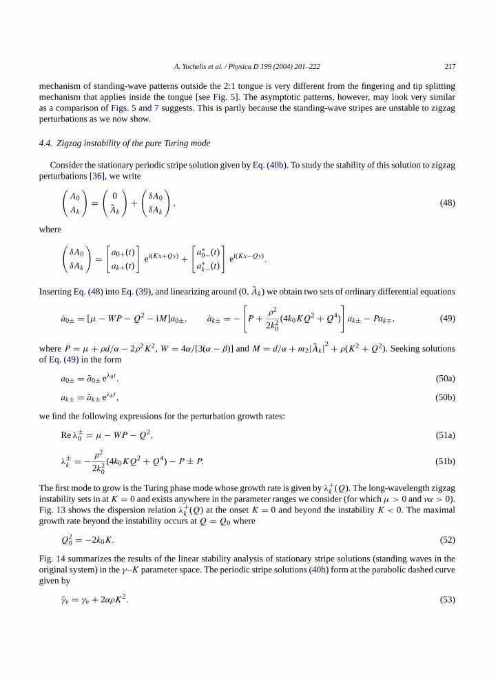
Fig. 12. Invasion of resonant standing waves into unlocked oscillations, obtained by numerical integration ofEq. (39) in the rangeγN < γ < γb.The solution represents the real part of (U0, V0) reconstructed according toEq. (30). Neumann boundary conditions were used. This behaviorreproduces the results ofFig. 7obtained by solvingEq. (6) with the same parameter values.
A. Yochelis et al. / Physica D 199 (2004) 201–222 217
mechanism of standing-wave patterns outside the 2:1 tongue is very different from the fingering and tip splittingmechanism that applies inside the tongue [seeFig. 5]. The asymptotic patterns, however, may look very similaras a comparison ofFigs. 5 and 7suggests. This is partly because the standing-wave stripes are unstable to zigzagperturbations as we now show.
4.4. Zigzag instability of the pure Turing mode
Consider the stationary periodic stripe solution given byEq. (40b). To study the stability of this solution to zigzagperturbations[36], we write(
A0
Ak
)=(
0
Ak
)+(δA0
δAk
), (48)
where
(δA0
δAk
)=[a0+(t)
ak+(t)
]ei(Kx+Qy) +
[a∗
0−(t)
a∗k−(t)
]ei(Kx−Qy).
InsertingEq. (48) into Eq. (39), and linearizing around (0, Ak) we obtain two sets of ordinary differential equations
a0± = [µ−WP −Q2 − iM]a0±, ak± = −[P + ρ2
2k20
(4k0KQ2 +Q4)
]ak± − Pak∓, (49)
whereP = µ+ ρd/α− 2ρ2K2, W = 4α/[3(α− β)] andM = d/α+m2|Ak|2 + ρ(K2 +Q2). Seeking solutionsof Eq. (49) in the form
a0± = a0± eλ0t , (50a)
ak± = ak± eλkt, (50b)
w
T giF lg
F s in theo rveg
e find the following expressions for the perturbation growth rates:
Reλ±0 = µ−WP −Q2, (51a)
λ±k = − ρ2
2k20
(4k0KQ2 +Q4) − P ± P. (51b)
he first mode to grow is the Turing phase mode whose growth rate is given byλ+k (Q). The long-wavelength zigza
nstability sets in atK = 0 and exists anywhere in the parameter ranges we consider (for whichµ > 0 andνα > 0).ig. 13shows the dispersion relationλ+
k (Q) at the onsetK = 0 and beyond the instabilityK < 0. The maximarowth rate beyond the instability occurs atQ = Q0 where
Q20 = −2k0K. (52)
ig. 14summarizes the results of the linear stability analysis of stationary stripe solutions (standing waveriginal system) in theγ–K parameter space. The periodic stripe solutions(40b) form at the parabolic dashed cuiven by
γe = γe + 2αρK2. (53)
218 A. Yochelis et al. / Physica D 199 (2004) 201–222
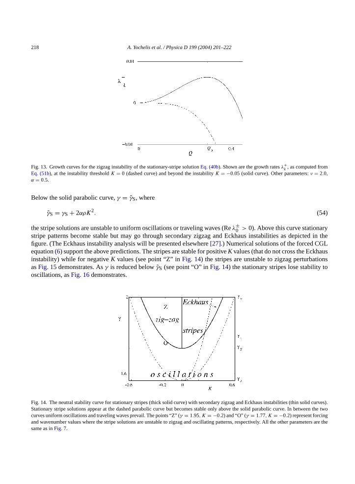
Fig. 13. Growth curves for the zigzag instability of the stationary-stripe solutionEq. (40b). Shown are the growth ratesλ+k
, as computed fromEq. (51b), at the instability thresholdK = 0 (dashed curve) and beyond the instabilityK = −0.05 (solid curve). Other parameters:ν = 2.0,α = 0.5.
Below the solid parabolic curve,γ = γS, where
γS = γS + 2αρK2. (54)
the stripe solutions are unstable to uniform oscillations or traveling waves (Reλ±0 > 0). Above this curve stationary
stripe patterns become stable but may go through secondary zigzag and Eckhaus instabilities as depicted in thefigure. (The Eckhaus instability analysis will be presented elsewhere[27].) Numerical solutions of the forced CGLequation(6) support the above predictions. The stripes are stable for positiveK values (that do not cross the Eckhausinstability) while for negativeK values (see point “Z” inFig. 14) the stripes are unstable to zigzag perturbationsasFig. 15demonstrates. Asγ is reduced belowγS (see point “O” inFig. 14) the stationary stripes lose stability tooscillations, asFig. 16demonstrates.
Fig. 14. The neutral stability curve for stationary stripes (thick solid curve) with secondary zigzag and Eckhaus instabilities (thin solid curves).Stationary stripe solutions appear at the dashed parabolic curve but becomes stable only above the solid parabolic curve. In between the twocurves uniform oscillations and traveling waves prevail. The points “Z” (γ = 1.95,K = −0.2) and “O” (γ = 1.77,K = −0.2) represent forcingand wavenumber values where the stripe solutions are unstable to zigzag and oscillating patterns, respectively. All the other parameters are thes
ame as inFig. 7.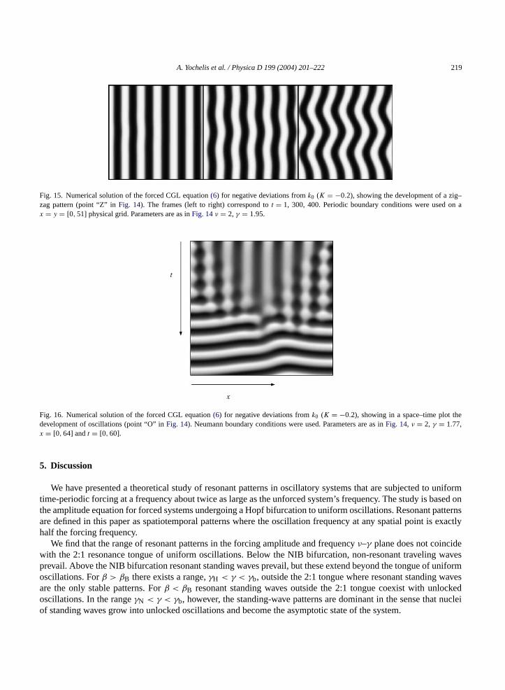
A. Yochelis et al. / Physica D 199 (2004) 201–222 219
Fig. 15. Numerical solution of the forced CGL equation(6) for negative deviations fromk0 (K = −0.2), showing the development of a zig–zag pattern (point “Z” inFig. 14). The frames (left to right) correspond tot = 1, 300, 400. Periodic boundary conditions were used on ax = y = [0,51] physical grid. Parameters are as inFig. 14ν = 2, γ = 1.95.
Fig. 16. Numerical solution of the forced CGL equation(6) for negative deviations fromk0 (K = −0.2), showing in a space–time plot thedevelopment of oscillations (point “O” inFig. 14). Neumann boundary conditions were used. Parameters are as inFig. 14, ν = 2, γ = 1.77,x = [0,64] andt = [0,60].
5. Discussion
We have presented a theoretical study of resonant patterns in oscillatory systems that are subjected to uniformtime-periodic forcing at a frequency about twice as large as the unforced system’s frequency. The study is based onthe amplitude equation for forced systems undergoing a Hopf bifurcation to uniform oscillations. Resonant patternsare defined in this paper as spatiotemporal patterns where the oscillation frequency at any spatial point is exactlyhalf the forcing frequency.
We find that the range of resonant patterns in the forcing amplitude and frequencyν–γ plane does not coincidewith the 2:1 resonance tongue of uniform oscillations. Below the NIB bifurcation, non-resonant traveling wavesprevail. Above the NIB bifurcation resonant standing waves prevail, but these extend beyond the tongue of uniformoscillations. Forβ > βB there exists a range,γH < γ < γb, outside the 2:1 tongue where resonant standing wavesare the only stable patterns. Forβ < βB resonant standing waves outside the 2:1 tongue coexist with unlockedoscillations. In the rangeγN < γ < γb, however, the standing-wave patterns are dominant in the sense that nucleiof standing waves grow into unlocked oscillations and become the asymptotic state of the system.
220 A. Yochelis et al. / Physica D 199 (2004) 201–222
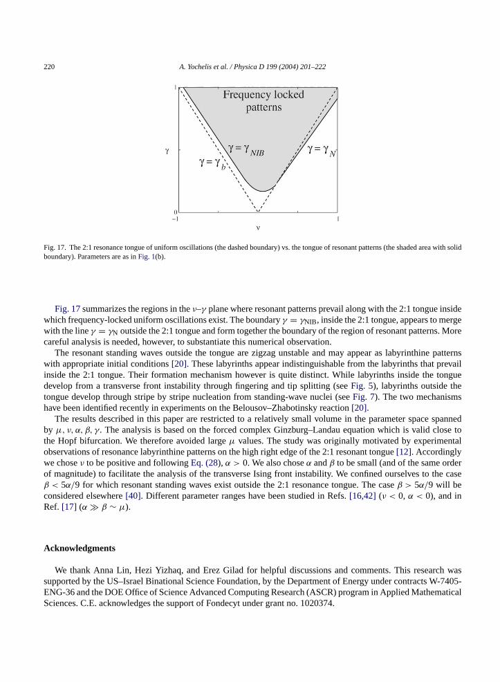
Fig. 17. The 2:1 resonance tongue of uniform oscillations (the dashed boundary) vs. the tongue of resonant patterns (the shaded area with solidboundary). Parameters are as inFig. 1(b).
Fig. 17summarizes the regions in theν–γ plane where resonant patterns prevail along with the 2:1 tongue insidewhich frequency-locked uniform oscillations exist. The boundaryγ = γNIB, inside the 2:1 tongue, appears to mergewith the lineγ = γN outside the 2:1 tongue and form together the boundary of the region of resonant patterns. Morecareful analysis is needed, however, to substantiate this numerical observation.
The resonant standing waves outside the tongue are zigzag unstable and may appear as labyrinthine patternswith appropriate initial conditions[20]. These labyrinths appear indistinguishable from the labyrinths that prevailinside the 2:1 tongue. Their formation mechanism however is quite distinct. While labyrinths inside the tonguedevelop from a transverse front instability through fingering and tip splitting (seeFig. 5), labyrinths outside thetongue develop through stripe by stripe nucleation from standing-wave nuclei (seeFig. 7). The two mechanismshave been identified recently in experiments on the Belousov–Zhabotinsky reaction[20].
The results described in this paper are restricted to a relatively small volume in the parameter space spannedby µ, ν, α, β, γ. The analysis is based on the forced complex Ginzburg–Landau equation which is valid close tothe Hopf bifurcation. We therefore avoided largeµ values. The study was originally motivated by experimentalobservations of resonance labyrinthine patterns on the high right edge of the 2:1 resonant tongue[12]. Accordinglywe choseν to be positive and followingEq. (28), α > 0. We also choseα andβ to be small (and of the same orderof magnitude) to facilitate the analysis of the transverse Ising front instability. We confined ourselves to the caseβ < 5α/9 for which resonant standing waves exist outside the 2:1 resonance tongue. The caseβ > 5α/9 will beconsidered elsewhere[40]. Different parameter ranges have been studied in Refs.[16,42] (ν < 0, α < 0), and inRef. [17] (α β ∼ µ).
Acknowledgments
We thank Anna Lin, Hezi Yizhaq, and Erez Gilad for helpful discussions and comments. This research wassupported by the US–Israel Binational Science Foundation, by the Department of Energy under contracts W-7405-ENG-36 and the DOE Office of Science Advanced Computing Research (ASCR) program in Applied MathematicalSciences. C.E. acknowledges the support of Fondecyt under grant no. 1020374.
A. Yochelis et al. / Physica D 199 (2004) 201–222 221
References
[1] V.I. Arnold, Geometrical Methods in the Theory of Ordinary Differential Equations, Springer-Verlag, New York, 1983.[2] M.H. Jensen, P. Bak, T. Bohr, Transition to chaos by interaction of resonances in dissipative systems. I. Circle maps, Phys. Rev. A 30
(1984) 1960–1969.[3] L. Glass, J. Sun, Periodic forcing of a limit-cycle oscillator : Fixed points, Arnold tongues, and the global organization of bifurcations,
Phys. Rev. E 50 (6) (1994) 5077–5084.[4] R.C. Hilborn, Chaos and Nonlinear Dynamics, Oxford University Press, New York, 1994.[5] J.A. Glazier, A. Libchaber, Quasi-periodicity and dynamical systems: an experimentalist’s view, IEEE Trans. Circuits Syst. 35 (1988)
790–809.[6] M. Eiswirth, G. Ertl, Forced oscillations of a self-oscillating surface reaction, Phys. Rev. Lett. 60 (15) (1988) 1526–1529.[7] P. Coullet, J. Lega, B. Houchmanzadeh, J. Lajzerowicz, Breaking chirality in nonequilibrium systems, Phys. Rev. Lett. 65 (1990) 1352–1355.[8] P. Coullet, K. Emilsson, Strong resonances of spatially distrubuted oscillatiors: a laboratory to study patterns and defects, Physica D 61
(1992) 119–131.[9] V. Petrov, Q. Ouyang, H.L. Swinney, Resonant pattern formation in a chemical system, Nature 388 (1997) 655–657.
[10] A.L. Lin, A. Hagberg, A. Ardelea, M. Bertram, H.L. Swinney, E. Meron, Four-phase patterns in forced oscillatory systems, Phys. Rev. E62 (2000) 3790–3798.
[11] H. Chate, A. Pikovsky, O. Rudzick, Forcing oscillatory media: phase kinks vs. synchronization, Physica D 131 (1999) 17–30.[12] A.L. Lin, M. Bertram, K. Martinez, H.L. Swinney, A. Ardelea, G.F. Carey, Resonant phase patterns in a reaction–diffusion system, Phys.
Rev. Lett. 84 (2000) 4240–4243.[13] V.K. Vanag, L.F. Yang, M. Dolnik, A.M. Zhabotinsky, I.R. Epstein, Oscillatory cluster patterns in a homogeneous chemical system with
global feedback, Nature 406 (6794) (2000) 389–391.[14] V.K. Vanag, A.M. Zhabotinsky, I.R. Epstein, Pattern formation in the Belousov–Zhabotinsky reaction with photochemical global feedback,
J. Phys. Chem. A 104 (49) (2000) 11566–11577.[15] V.K. Vanag, A.M. Zhabotinsky, I.R. Epstein, Oscillatory clusters in the periodically illuminated, spatially extended Belousov–Zhabotinsky
reaction, Phys. Rev. Lett. 86 (3) (2001) 552–555.[16] H.-K. Park, Frequency locking in spatially extended systems, Phys. Rev. Lett. 86 (2001) 1130–1133.[17] D. Gomila, P. Colet, G.L. Oppo, M.S. Miguel, Stable droplets and growth laws close to the modulational instability of a domain wall, Phys.
Rev. Lett. 87 (19) (2001) 194101.[18] R. Gallego, D. Walgraef, M. San Miguel, R. Toral, Transition from oscillatory to excitable regime in a system forced at three times its
natural frequency, Phys. Rev. E 64 (5) (2001) 056218.[19] J. Kim, J. Lee, B. Kahng, Harmonic forcing of an extended oscillatory system: Homogeneous and periodic solutions, Phys. Rev. E 65 (4)
(2002) 046208.[20] A. Yochelis, A. Hagberg, E. Meron, A.L. Lin, H.L. Swinney, Development of standing-wave labyrinthine patterns, SIADS 1 (2) (2002)
236–247http://epubs.siam.org/sam-bin/dbq/article/39711.[ ysica D
[ 30.[[ (1987)
[ ) (1998)
[ 85–5291.[[ 7 (1994)
[[ 55–258.[ 33–37.[ rametric
[ sica
[[
21] K. Martinez, A.L. Lin, R. Kharrazian, X. Sailer, H.L. Swinney, Resonance in periodically inhibited reaction–diffusion systems, Ph2 (2002) 168–169.
22] E. Meron, Phase fronts and synchronization patterns in forced oscillatory systems, Discrete Dyn. Nat. Soc. 4 (3) (2000) 217–223] J.M. Gambaudo, Perturbation of a Hopf bifurcation by an external time-periodic forcing, J. Diff. Eq. 57 (1985) 172–199.24] C. Elphick, G. Iooss, E. Tirapegui, Normal form reduction for time-periodically driven differential equations, Phys. Lett. A 120
459–463.25] C. Elphick, A. Hagberg, E. Meron, A phase front instability in periodically forced oscillatory systems, Phys. Rev. Lett. 80 (22
5007–5010.26] C. Elphick, A. Hagberg, E. Meron, Multiphase patterns in periodically forced oscillatory systems, Phys. Rev. E 59 (5) (1999) 5227] A. Yochelis, Pattern formation in periodically forced oscillatory systems, Ph.D. Thesis, Ben-Gurion University, 2003.28] A. Hagberg, E. Meron, Pattern formation in non-gradient reaction–diffusion systems: the effects of front bifurcations, Nonlinearity
805–835.29] A. Hagberg, E. Meron, From labyrinthine patterns to spiral turbulence, Phys. Rev. Lett. 72 (15) (1994) 2494–2497.30] S. Sarker, S.E. Trullinger, A.R. Bishop, Solitary-wave solution for a complex one-dimensional field, Phys. Lett. A 59 (4) (1976) 231] C. Elphick, A. Hagberg, E. Meron, B. Malomed, On the origin of traveling pulses in bistable systems, Phys. Lett. A 230 (1997)32] D.V. Skryabin, A. Yulin, D. Michaelis, W.J. Firth, G.L. Oppo, U. Peschel, F. Lederer, Perturbation theory for domain walls in the pa
Ginzburg–Landau equation, Phys. Rev. E 64 (5) (2001) 056618.33] C. Elphick, Dynamical approach to the Ising-Bloch transition in 3 + 1dimensional time periodically driven dynamical systems, Phy
D, submitted for publication.34] A.C. Newell, J.A. Whitehead, Finite bandwidth, finite amplitude convection, J. Fluid Mech. 38 (1969) 279–303.35] L.A. Segel, Distant side-walls cause slow amplitude modulation of cellular convection, J. Fluid Mech. 38 (1969) 203–224.
222 A. Yochelis et al. / Physica D 199 (2004) 201–222
[36] M.C. Cross, P.C. Hohenberg, Pattern formation outside of equilibrium, Rev. Mod. Phys. 65 (3) (1993) 851–1112.[37] J.P. Keener, Secondary bifurcation in nonlinear diffusion-reaction equations, Stud. Appl. Math. 55 (3) (1976) 187–211.[38] H. Kidachi, On mode interactions in reaction diffusion equation with nearly degenerate bifurcations, Prog. Theor. Phys. 63 (4) (1980)
1152–1169.[39] J.D. Crawford, Introduction to bifurcation theory, Rev. Mod. Phys. 63 (4) (1991) 991–1037.[40] A. Yochelis, C. Elphick, A. Hagberg, E. Meron, Frequency locking in extended systems: the impact of a Turing mode, in press.[41] M. Or-Guil, M. Bode, Propagation of Turing–Hopf fronts, Physica A 249 (1998) 174–178.[42] H.-K. Park, M. Bär, Spiral destabilization by resonant forcing, Europhys. Lett. 65 (2004) 873–879.