Two serve and project - in more ways: two-way analysis of

Two serve and project - in more ways: two-wayanalysis of variance with random effects

Rasmus WaagepetersenDepartment of Mathematics

Aalborg UniversityDenmark

March 3, 2021

1 / 31

Outline for today

I Two-way ANOVA using orthogonal projections

2 / 31

Two-way ANOVAConsider two factors: T (treatment) and P (plot) with number oflevels dT and dP . Moreover let P × T be the cross-factor (hasdPdT levels - one for each combination of levels of P and T ).

Assume P × T is balanced with nP×T = m observations for eachlevel. Then P and T balanced too with numbers of observationsnP = mdT and nT = mdP for each level.

Model with random P and P × T effects (e.g. to account for soilvariation)

yptr = ξ + βt + Up + Upt + εptr

p = 1, . . . , dP , t = 1, . . . , dT , r = 1, . . . ,m

In vector form:

y = µ+ ZPUP + ZP×TUP×T + ε

where µ ∈ LT = spanXT .3 / 31

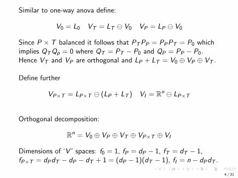
Similar to one-way anova define:

V0 = L0 VT = LT V0 VP = LP V0

Since P × T balanced it follows that PTPP = PPPT = P0 whichimplies QTQp = 0 where QT = PT − P0 and QP = PP − P0.Hence VT and VP are orthogonal and LP + LT = V0 ⊕ VP ⊕ VT .

Define further

VP×T = LP×T (LP + LT ) VI = Rn LP×T

Orthogonal decomposition:

Rn = V0 ⊕ VP ⊕ VT ⊕ VP×T ⊕ VI

Dimensions of ‘V ’ spaces: f0 = 1, fP = dP − 1, fT = dT − 1,fP×T = dPdT − dP − dT + 1 = (dP − 1)(dT − 1), fI = n − dPdT .

4 / 31

Orthogonal projections on ‘V ’ spaces: Q0 = P0, QP = PP − Q0,QT = PT − Q0, QP×T = PP×T − QP − QT − Q0 andQI = I − PP×T .

Covariance structure:

CovY = σ2PnPPP + σ2P×TnP×TPP×T + σ2I

= λPQP + λP×T QP×T + λI QI

where

λI = σ2

λP×T = σ2 + nP×Tσ2P×T

λP = σ2 + nP×Tσ2P×T + nPσ

2P

and

QP = Q0 + QP = PP QP×T = QP×T + QT QI = QI

5 / 31

Interpretation of VP×T for a fixed effects two-way ANOVA

Suppose that P and T are both systematic factors. Then theordinary two-way ANOVA is

yptr = ξ + αp + βt + γpt + εptr .

Then LP×T is the space for the mean vectorµ = (ξ + αp + βt + γpt)ptr .

Similarly, LP + LT is the space for the mean vectorµ = (ξ + αp + βt)ptr in case of the additive model where theγpt = 0 (no interaction).

Hence VP×T = LP×T (LP + LT ) is the ‘interaction space’.

6 / 31

‘Q’s are orthogonal projections on

VP = V0 + VP VP×T = VP×T + VT VI = VI

This corresponds to orthogonal decomposition

Rn = VP ⊕ VP×T ⊕ VI

based on model without systematic effects (‘V ’-spaces aggregatedinto V -spaces).

7 / 31

Orthogonal decomposition of data vector:

Y = Q0Y + QPY + QTY + QP×TY + QIY

= QPY + QP×TY + QIY

Decomposition of mean vector µ ∈ LT = V0 ⊕ VT :

µ = QPµ+ QP×Tµ+ QIµ = Q0µ+ QTµ+ 0 = µ0 + µT

where µ0 ∈ L0 and µT ∈ VT .

Note: one-to-one correspondence between µ and (µ0,µT )(reparametrization)

8 / 31

As for one-way anova Y is decomposed into independent normalvectors

QPY ∼ N(µ0, λPQP) QP×TY ∼ N(µT , λP×T QP×T )

QIY ∼ N(0, λI QI )

Density for Y factorizes into product of ‘densities’ for QPY ,QP×TY and QIY .

Hence

µ0 = P0QPY = P0Y = Y··1n µT = QT QP×TY = QTY

µ = µ0 + µT = PTY λP = ‖QPY − P0Y ‖2/dP = ‖QPY ‖2/dPλP×T = ‖QP×TY−QTY ‖2/(dPdT−dP) = ‖QP×TY ‖2/(dPdT−dP)

λI = σ2 = ‖QIY ‖2/(n − dPdT )

NB: since VP and VP×T have dimensions fP = dP − 1 andfP×T = (dP − 1)(dT − 1) we often use these denominators insteadof dP and dPdT − dP for λP and λP×T (REML).Note: MLE for µ is identical to MLE in the linear model withµ ∈ LT and no random effects.

9 / 31

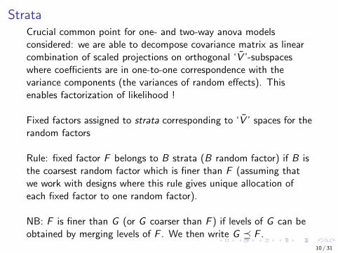
StrataCrucial common point for one- and two-way anova modelsconsidered: we are able to decompose covariance matrix as linearcombination of scaled projections on orthogonal ‘V ’-subspaceswhere coefficients are in one-to-one correspondence with thevariance components (the variances of random effects). Thisenables factorization of likelihood !

Fixed factors assigned to strata corresponding to ‘V ’ spaces for therandom factors

Rule: fixed factor F belongs to B strata (B random factor) if B isthe coarsest random factor which is finer than F (assuming thatwe work with designs where this rule gives unique allocation ofeach fixed factor to one random factor).

NB: F is finer than G (or G coarser than F ) if levels of G can beobtained by merging levels of F . We then write G � F .

10 / 31

Structure diagram

I PxT

P

T

O

Arrow from F to G if G is coarser than F and there is nointermediate factor which is coarser than F and finer than G .

Note: three strata (black, green and red) corresponding to‘random’ factors I , P × T and P.

NB: here we can not have both P and T random unless O randomtoo (if O systematic no unique allocation to random factor strata).Also want to respect hierarchical principle so P × T can not befixed if P random.

11 / 31

Relation to ‘old school ANOVA’By orthogonal decomposition

Y = Q0Y + QPY + QTY + QP×TY + QIY

and Pythagoras,

‖Y − Q0Y ‖2 = ‖QPY ‖2 + ‖QTY ‖2 + ‖QP×TY ‖2 + ‖QIY ‖2

With terminology SSF=‖QFY ‖2 we get∑ptr

(Yptr − Y···)2 = SSP + SST + SSPT + SSI

Here, for example, SSP=∑

ptr (Yp·· − Y···)2 and SSPT=∑

ptr (Ypt· − Yp·· − Y·t· + Y···)2.

Sorry: in relation with one-way ANOVA I called left hand side SST(T for total) and SSI was SSE

12 / 31

Note also: QTY = (Y·t· − Y···)ptr .

This is the part of the mean vector that corresponds to sum tozero constraint: with

βt = Y·t· − Y···

we have ∑t

βt = 0

13 / 31

Paper pulp example: two-way analysis of variance withouttreatment effect

P: card board with dP = 5. T: position within cardboard (not atreatment) with dT = 4. Number of replications m = 4.

Model:yptr = ξ + Up + Upt + εptr

Variances σ2P , σ2P×T and σ2

We can use exactly the same orthogonal decomposition as before.Only difference is that QTµ = QT1nξ = 0 which meansQP×TY ∼ N(0, λP×T QP×T ) and REML and ML estimates forλP×T coincide and are equal to

λP×T = ‖QP×TY ‖2/(dPdT − dP)

NB: in ANOVA table (next slide), SSP=‖QPY ‖2, SST=‖QTY ‖2,SSPT=‖QP×TY ‖2 and SSE=‖QIY ‖2.

14 / 31

ANOVA table

Analysis of Variance Table

Response: Reflektans

Df Sum Sq Mean Sq F value Pr(>F)

factor(Sted) 3 0.03600 0.011999 188.981 < 2.2e-16 ***

#SST

factor(Pap.nr.) 4 1.07520 0.268800 4233.472 < 2.2e-16 ***

#SSP

factor(Sted):factor(Pap.nr.)

12 0.02168 0.001807 28.452 < 2.2e-16 ***

#SSPT

Residuals 60 0.00381 0.000063

#SSE

σ2 = 0.00006 λP×T = (0.036 + 0.02168)/15 = 0.00385λP = 1.0752/5 = 0.21504 (or λP = 1.0752/4 = 0.0072 = 0.2688).

15 / 31

By relations

λP×T = σ2 + nP×Tσ2P×T

λP = σ2 + nP×Tσ2P×T + nPσ

2P

we obtain σ2P = (0.21504− 0.00385)/16 = 0.0132σ2P×T = (0.00385− 0.00006)/4 = 0.0009475 (orσ2P = (0.2688− 0.00385)/16 = 0.01655937)

Recall: balanced design required - and difficult to remember rulesfor calculating variance components.

16 / 31

Using lmer and ML

> out2=lmer(Reflektans~(1|Sted:Pap.nr.)+(1|Pap.nr.),REML=F)

> summary(out2)

Random effects:

Groups Name Variance Std.Dev.

Sted:Pap.nr. (Intercept) 9.454e-04 0.030747

Pap.nr. (Intercept) 1.320e-02 0.114890

Residual 6.349e-05 0.007968

Number of obs: 80, groups: Sted:Pap.nr., 20; Pap.nr., 5

17 / 31

Using lmer and REML

> out2=lmer(Reflektans~(1|Sted:Pap.nr.)+(1|Pap.nr.))

> summary(out2)

Random effects:


Sted:Pap.nr. (Intercept) 9.455e-04 0.030749

Pap.nr. (Intercept) 1.657e-02 0.128717

Residual 6.349e-05 0.007968

Number of obs: 80, groups: Sted:Pap.nr., 20; Pap.nr., 5

Note REML and ML estimates for σ2 and σ2P×T coincide (up torounding error)

18 / 31

Explanation of Reflektans~(1|Sted:Pap.nr.)+(1|Pap.nr.)):

I no fixed formula: intercept always included as default

I (1|Sted:Pap.nr.) random intercepts for groups identifiedby variable StedPap.nr.

I (1|Pap.nr.) random intercepts for groups identified byvariable Pap.nr.

I random effects specified by different terms independent.

19 / 31

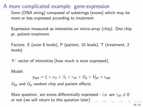
A more complicated example: gene-expressionGene (DNA string) composed of substrings (exons) which may bemore or less expressed according to treatment.

Expression measured as intensities on micro-array (chip). One chippr. patient-treatment.

Factors: E (exon 8 levels), P (patient, 10 levels), T (treatment, 2levels)

Y : vector of intensities (how much is exon expressed).

Model:yept = ξ + αe + βt + γet + Up + Upt + εept

Upt and Up random chip and patient effects.

Main question: are exons differentially expressed - i.e. are γet 6= 0or not (we will return to this question later)

20 / 31

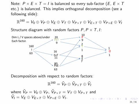
Note: P × E × T = I is balanced so every sub-factor (E , E × Tetc.) is balanced. This implies orthogonal decomposition (see afollowing slide):

R160 = V0 ⊕ VP ⊕ VE ⊕ VT ⊕ VP×T ⊕ VE×T ⊕ VP×E ⊕ VI

Structure diagram with random factors P,P × T , I :

I

PxTP

T

O

EExT

PxE

Dim L / V spaces above/underEach factor.

1

1

10

9

2

1

8

7

20

9

16

11

80

63

160

63

Decomposition with respect to random factors:

R160 = VP ⊕ VP×T ⊕ VI

where VP = V0 ⊕ VP , VP×T = VT ⊕ VP×T andVI = VE ⊕ VE×T ⊕ VP×E ⊕ VI .

21 / 31

Decomposition of CovY :

CovY = nPσ2PPP+nP×Tσ

2P×TPP×T+σ2I = λPQP+λP×T QP×T+λI QI

Decomposition of µ:

µ = QPµ+ QP×Tµ+ QIµ = Q0µ+ QTµ+ QEµ+ QE×Tµ

As before decomposition of Y into independent Gaussian vectors:

QPY ∼ N(Q0µ, λPQP) QP×TY ∼ N(QTµ, λP×T QP×T )

QIY ∼ N((QE + QE×T )µ, λI QI

)

22 / 31

Orthogonality of ‘V ’-spacesWe use results of exercise 5 to deduce that

PP×EPE×T = PE QPPE×T = PPPE×T −P0PE×T = P0−P0 = 0

The second equality shows that VP and VE×T are orthogonal.

Further:

QP×E = PP×E −QP −QE −Q0 QE×T = PP×E −QE −QT −Q0

Using the result in the upper equation and pairwise orthogonalityof QP ,QE ,QT ,Q0 we get

QP×EQE×T = 0

Thus VP×E and VE×T are orthogonal too.

Orthogonality of VP×T , VP and VT was shown for two-wayANOVA.

Proceeding this way all ‘V ’ spaces orthogonal.23 / 31

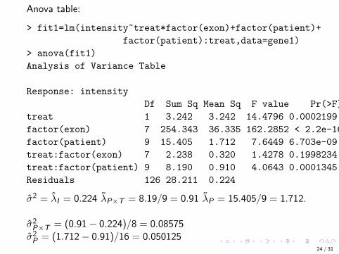
Anova table:

> fit1=lm(intensity~treat*factor(exon)+factor(patient)+

factor(patient):treat,data=gene1)

> anova(fit1)

Analysis of Variance Table

Response: intensity


treat 1 3.242 3.242 14.4796 0.0002199 ***

factor(exon) 7 254.343 36.335 162.2852 < 2.2e-16 ***

factor(patient) 9 15.405 1.712 7.6449 6.703e-09 ***

treat:factor(exon) 7 2.238 0.320 1.4278 0.1998234

treat:factor(patient) 9 8.190 0.910 4.0643 0.0001345 ***

Residuals 126 28.211 0.224

σ2 = λI = 0.224 λP×T = 8.19/9 = 0.91 λP = 15.405/9 = 1.712.

σ2P×T = (0.91− 0.224)/8 = 0.08575σ2P = (1.712− 0.91)/16 = 0.050125

24 / 31

With aov()

> fit1=aov(intensity~treatment*factor(exon)+

Error(factor(patient)+factor(patient):treatment),data=gene1)

> summary(fit1)

Error: factor(patient)


Residuals 9 15.4 1.712

Error: factor(patient):treatment


treatment 1 3.242 3.242 3.563 0.0917 .

Residuals 9 8.190 0.910

---

Signif. codes: 0 ‘***’ 0.001 ‘**’ 0.01 ‘*’ 0.05 ‘.’ 0.1 ‘ ’ 1

Error: Within


factor(exon) 7 254.34 36.33 162.285 <2e-16 ***

treatment:factor(exon) 7 2.24 0.32 1.428 0.2

Residuals 126 28.21 0.22

---

Signif. codes: 0 ‘***’ 0.001 ‘**’ 0.01 ‘*’ 0.05 ‘.’ 0.1 ‘ ’ 1

Conveniently organizes factors into strata !

25 / 31

Using lmer:

> fit1=lmer(intensity~treat*factor(exon)+

(1|patient)+(1|patient:treatment),data=gene1)

> summary(fit1)

Random effects:


patient:treatment (Intercept) 0.08577 0.2929

patient (Intercept) 0.05011 0.2239

Residual 0.22389 0.4732

Number of obs: 160, groups: patient:treatment, 20; patient, 10

26 / 31

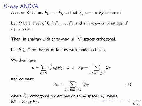
K -way ANOVAAssume K factors F1, . . . ,FK so that F1 × . . .× FK balanced.

Let D be the set of 0, I ,F1, . . . ,FK and all cross-combinations ofF1, . . . ,FK .

Then, in analogy with three-way, all ’V’ spaces orthogonal.

Let B ⊆ D be the set of factors with random effects.

We then have

Σ =∑B∈B

σ2BnBPB and PB =∑

F∈D:F�BQF

and we wantPB =

∑B′∈B:B′�B

QB′ (1)

where QB orthogonal projections on some spaces VB whereRn = ⊗B∈BVB .

27 / 31

K -way ANOVA continuedGiven (1) we have required decomposition of Σ into sum of scaledorthogonal projections:

Σ =∑B∈B

σ2BnBPB =∑B′∈B

λB′QB′ where λB′ =∑

B∈B:B′�BnBσ

2B .

A sufficient (and necessary) condition for (1) is that: for all F ∈ Dthere exists a B ∈ B such that F � B and B � B ′ for all other B ′

with F � B ′.

(this must be checked for a given model. Note this implies I ∈ Band that B = B(F ) is unique).

Then we define

VB =∑

F∈D:B(F )=B

VF and QB =∑

F∈D:B(F )=B

QF

Each F ∈ D belongs to precisely one VB so Rn = ⊗B∈BVB .28 / 31

K -way ANOVA continued

Thus we can again obtain decomposition Y of into independentYB = QBY , B ∈ B.

See also more details in note “Analysis of variance usingorthogonal projections”.

Even more general set-up can be found in Jesper Møller: Centralestatistiske modeller og likelihood baserede metoder.

29 / 31

Exercises

1. Check that PTPP = P0.

2. Check that LT + LP = V0 ⊕ VP ⊕ VT .

3. Derive factorization of likelihood for balanced two-way. Deriveestimates of mean and variance parameters.

4. Install the R-package faraway which contains the data setpenicillin. The response variable is yield of penicillin forfour different production processes (the ‘treatment’). The rawmaterial for the production comes in batches (‘blends’). Thefour production processes were applied to each of the 5blends. Fit anova models with production process as a fixedfactor and blend as random factor. Try to use both the anovatable and lmer.

30 / 31

5. In a balanced three-way design with factors F1,F2, and F3show that

PF1×F2PF2×F3 = PF2 PF1×F2PF3 = P0

Explain how this can be generalized to the following result:

P∏i∈A Fi

P∏i∈B Fi

= P∏i∈A∩B Fi

for a K -way balanced design with factors Fi , i = 1, . . . ,K andA,B ⊆ {1, . . . ,K} (taking P∏

i∈∅Fi= P0).

31 / 31

Documents

Two serve and project - in more ways: two-way analysis of