CURVE is the Institutional Repository for Coventry University

Tyre model development using co-simulation technique for helicopter ground operation Wang, Y. , Blundell, M. V. , Woodand, G. and Bastien, C. J. Author post-print (accepted) deposited in CURVE January 2016 Original citation & hyperlink: Wang, Y. , Blundell, M. V. , Woodand, G. and Bastien, C. J. (2014) Tyre model development using co-simulation technique for helicopter ground operation. Proceedings of the Institution of Mechanical Engineers, Part K: Journal of Multi-body Dynamics, volume 228 (4): 400-413 http://dx.doi.org/10.1177/1464419314541638 ISSN 1464-4193 ESSN 2041-3068 DOI 10.1177/1464419314541638 Copyright © and Moral Rights are retained by the author(s) and/ or other copyright owners. A copy can be downloaded for personal non-commercial research or study, without prior permission or charge. This item cannot be reproduced or quoted extensively from without first obtaining permission in writing from the copyright holder(s). The content must not be changed in any way or sold commercially in any format or medium without the formal permission of the copyright holders. This document is the author’s post-print version, incorporating any revisions agreed during the peer-review process. Some differences between the published version and this version may remain and you are advised to consult the published version if you wish to cite from it.

Mechanical, Automotive and Manufacturing

Engineering Department, Coventry University,

UK

Corresponding Author:

Yun Wang, Mechanical, Automotive and

Manufacturing Engineering Department,

Coventry University, Priory Street, Coventry,

CV1 5FB, UK

Email: wangy21@uni.coventry.ac.uk

Tyre Model Development Using Co-Simulation

Technique for Helicopter Ground Operation

Yun Wang, M V Blundell, G Wood and C Bastien

Vehicle Dynamics and Safety Applied Research Group, Coventry University, UK.

Abstract

This paper describes the development of a new aircraft tyre model applied using

a co-simulation approach for the multibody dynamic simulation of helicopter ground

vehicle dynamics. The new tyre model is presented using a point follower approach

that makes a novel contribution to this area by uniquely combining elements of two

existing tyre models used by the aircraft industry, namely the NASA R64 model

developed by Smiley and Horne [1] and the ESDU (Engineering Sciences Data Unit)

Mitchell tyre model [2].

Before the tyre model was used with a full helicopter model, a virtual tyre

test rig was used to examine the tyre and to predict the tyre forces and moments

for a range of tyre states. The paper concludes by describing the successful

application of the new tyre model with a full helicopter model and the simulation

of representative landing, take-off and runway taxiing manoeuvres. The predictive

capability of the model is demonstrated to show the open-loop ground vehicle

dynamics response of the helicopter and also the ground load predictive capability

for the distribution of loads through the tyres, wheels and landing gears.

Keywords: Multibody Dynamics, Helicopter Ground Dynamics, Tyre

Mechanics, Tyre Dynamics, Tyre Modelling, Landing Gears.

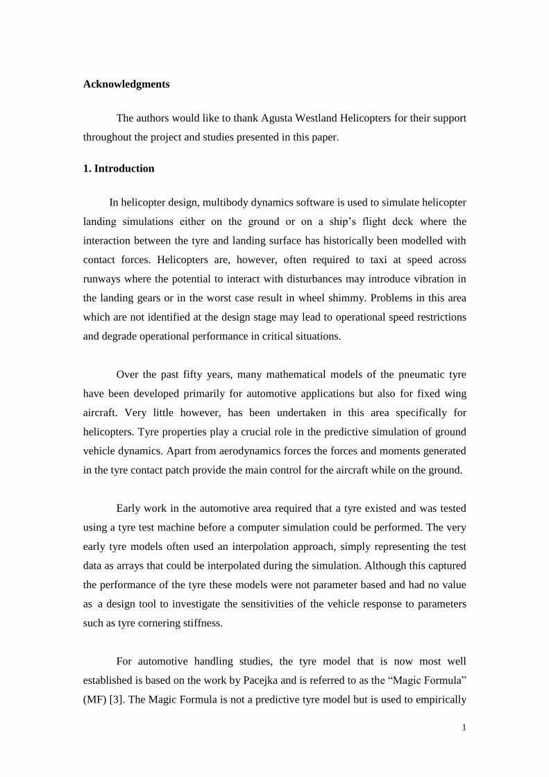
Nomenclature

A1, A2 – vertical force coefficient

B1 to B5 – cornering power coefficients

C1, C2 – tyre yaw angle parameter

Cz – coefficient in expression for tyre deflection under normal load

Cc – coefficient in expression for N

D – tyre diameter

D1 – lateral force coefficient

E1 to E4 – aligning moment coefficients

h – half length of tyre ground contact area

N – cornering power

n – user define coefficient

p – tyre pressure

pr – rated tyre pressure

Ru – unloaded radius

Rl – actual radius 𝑅𝑙 = 𝑅𝑢 + 𝛿

Re – effective radius

w – width of the tyre

Wz – steering angle

Z – normal load

δ – tyre vertical deflection

σ – relaxation length

Φ – tyre yaw-angle parameter

Ψtyre – tyre yaw (or slip) angle

λ0 – lateral distortion at the wheel centre

λ1 – lateral distortion one step before the contact patch centre

λ2 – lateral distortion one step after the contact patch centre

µΨ – coefficient of friction

µΨ max – maximum attainable value of force or friction coefficient in unbraked

yawed rolling and in braked unyawed rolling

µr – ratio between µΨ max and dry road friction coefficient

1

Acknowledgments

The authors would like to thank Agusta Westland Helicopters for their support

throughout the project and studies presented in this paper.

1. Introduction

In helicopter design, multibody dynamics software is used to simulate helicopter

landing simulations either on the ground or on a ship’s flight deck where the

interaction between the tyre and landing surface has historically been modelled with

contact forces. Helicopters are, however, often required to taxi at speed across

runways where the potential to interact with disturbances may introduce vibration in

the landing gears or in the worst case result in wheel shimmy. Problems in this area

which are not identified at the design stage may lead to operational speed restrictions

and degrade operational performance in critical situations.

Over the past fifty years, many mathematical models of the pneumatic tyre

have been developed primarily for automotive applications but also for fixed wing

aircraft. Very little however, has been undertaken in this area specifically for

helicopters. Tyre properties play a crucial role in the predictive simulation of ground

vehicle dynamics. Apart from aerodynamics forces the forces and moments generated

in the tyre contact patch provide the main control for the aircraft while on the ground.

Early work in the automotive area required that a tyre existed and was tested

using a tyre test machine before a computer simulation could be performed. The very

early tyre models often used an interpolation approach, simply representing the test

data as arrays that could be interpolated during the simulation. Although this captured

the performance of the tyre these models were not parameter based and had no value

as a design tool to investigate the sensitivities of the vehicle response to parameters

such as tyre cornering stiffness.

For automotive handling studies, the tyre model that is now most well

established is based on the work by Pacejka and is referred to as the “Magic Formula”

(MF) [3]. The Magic Formula is not a predictive tyre model but is used to empirically

2

represent previously measured tyre force and moment curves. The first version

developed is sometimes referred to as the “Monte Carlo version” due to the

conference location at which this model was presented in the 1989 paper.

The Magic Formula model is undergoing continual development, which is

reflected in a further publication where the model is not restricted to small values of

slip angle and the wheel may also run backwards. The authors also discuss a relatively

simple model for longitudinal and lateral transient responses restricted to relatively

low time and path frequencies. The tyre model in this paper also acquired a new name

and was referred to as the ‘Delft Tyre 97’ version, which has reverted over time to

MF-Tyre 5.0. Also the “Delft-Tyre” model has become an umbrella term to include

not only the base MF-Tyre model but a modified version of it suitable for

intermediate frequency events known [4].

Although the Magic Formula is widely used in the automotive and aircraft

sector (including helicopters), its capability is constantly face against different range

of challenges. Aircraft taxiing manoeuvres can lead to much larger slip angles (also

referred to as yaw angles) than those on automotive vehicles. While car tyres may

typically operate with slip angles of less than 10 degrees, even during severe

manoeuvres, for this particular investigation the helicopter tyres were subject to slip

angles up to 90 degrees. It is important to predict the carcass elasticity and transient

behaviour in manoeuvres such as cornering, braking and taxiing. Aircraft and

helicopters also often use bias tyres rather than the radial tyres established in the

automotive sector. In general the main problem in aerospace applications is the

absence of large scale tyre test programmes and a resulting lack of tyre test data. This

renders models such as the MF tyre model, although proven to be accurate, difficult to

use due to the large model parameter sets and the amount of experimental data

required to populate these. The aim of this project was therefore to develop a tyre

model with relatively low data input requirements. However, the model still needed to

capture most of the tyre dynamic behaviour and to be compatible with a range of

simulation scenarios.

The tyre model developed in this project was tested using a virtual tyre test rig

model developed in a multibody systems environment in order to support the

3

theoretical development of the model. Trial data sets were used to produce typical

graphs of tyre forces and moments as a function of vertical force and slip angle.

Finally a full scale helicopter model was developed and used to successfully

demonstrate the ground dynamics of the helicopter and the load prediction capability

for landing, takeoff and taxiing manoeuvres.

2. Review of Existing Tyre Models

Over the past fifty years, several approaches have been taken to develop

mathematical models to predict tyre behaviour. The tyre properties play a crucial role

when determining vehicle dynamic behaviour, due to the fact that tyres are the only

component which makes contact with the ground and provide the most significant

input to control vehicle motion and trajectory. There are in the main three different

categories of tyre models:

Analytical Models: the modelling of tyre/road contact was developed before the

1980s and mainly involves a point contact method, rigid tread band model and fixed

footprint model. Despite this, some of these models can only achieve relatively low

accuracy. However, they provided fundamental knowledge of the principal

characteristics of the tyre and contribute to the analytical components of a terrain-

vehicle interaction model used for dynamic vehicle simulation. These models include:

Brush Models - These models are based on a relatively simple representation of

the tyre structure where the model assumes the tyre to behave like an elastic

element. The tyre tread is represented by an array of small elastic rectangular

elements attached to a rigid ring. Each of the small elements possesses mass and

captures the transient effects introduced by the previous element as they enter in

and out of the contact patch [5]. This model has also been expanded upon by

Mavros [6] where the model includes viscoelastic circumferential connections

between the sequential bristles introducing a lateral degree of freedom. The

instantaneous state of the bristle depends on the state of the same bristle at the

preceding time step, as well as on the state of the two adjacent bristles at the same

time. A comparison was undertaken between the simple and expanded version of

4

the brush model and the results showed that the extended version can capture

certain oscillations such as the tyre transition from elastic deformation to the

slipping phase.

Gim and Nikravesh [7-9] have also conducted a detailed study for the

development of an analytical model of a pneumatic tyre. The first part of the

study included a brief review on tyre characteristics along with several algorithms

for computational modelling purposes. The second part of the study focused on

an analytical approach for determining tyre dynamic properties. The equations

derived in these papers describe a mathematical model for calculating the

principle forces and moments of a tyre. For the final part of the study the

analytical formulations were derived for the tyre dynamic properties as a function

of the slip ratio, slip angle, camber angle and other tyre dynamic parameters.

These formulations can be used for the general vehicle simulations in different

terrain conditions. The tyre model results were also compared with experimental

results. The analytical predictions of the longitudinal and lateral forces show

good agreement with the experimental values.

Harty Model - This model was developed to increase the accuracy and potential

of a low parameter tyre model. The model is similar in structure to the Fiala tyre

model, but has been significantly developed by incorporating new methods to

eliminate the major limitations in the Fiala tyre model. Improvements have been

made to the longitudinal and lateral force calculations along with better curve

fitting methods that have been utilised by introducing a series of scale factors

[10].

Semi-Empirical/Empirical Models: In order to improve the accuracy problem

caused by simplification in analytical modelling, semi-empirical/empirical models

have been developed. These models are developed using experimental data; the

formulation compensates for the margin of error introduced by theoretical

assumptions in analytical methods. Several classical empirical models have been

developed and are still being used for current tyre dynamic analysis.

5

Magic Formula - This is a widely used tyre model which permits the calculation

of the tyre forces and moments in various conditions. In Pacejka’s early research,

several types of mathematical functions were used to represent the cornering

force characteristics. Different equations such as exponential, arctangent,

parabolic and hyperbolic tangent functions were investigated to successfully

model the tyre dynamic characteristics. There are several versions of the Magic

Formula in which its use is extended to combined longitudinal, lateral slip and

camber angle within a simulation. The equations derived include a number of

micro-coefficients which have to be determined from experimental data. The

model provides simulation results that better fit the measured data. The Magic

Formula tyre model has wide spread use today and is constantly evolving [3]. The

model was further expanded to adopt higher frequency response and this version

is called the SWIFT (Short Wavelength Intermediate Frequency Tyre) tyre

model. The SWIFT tyre model is based upon the Magic Formula. The SWIFT

tyre model is able to describe dynamic tyre behaviour for in-plane (longitudinal

and vertical) and out-of-plane (lateral, camber and steering) motions up to about

60Hz, whilst also being able to accommodate road obstacles with short

wavelength. Due to accuracy and calculation speed the SWIFT model has been

programmed as a semi-empirical model which is derived using advanced physical

models and a dedicated high frequency tyre measurement to assess the speed

effects in tyre behaviour [4].

FTire Model - The FTire model is a flexible ring tyre model developed by

Gipser [11]. It is a full 3D nonlinear in-plane and out-of plane tyre simulation

model. It is designed for vehicle comfort simulations and prediction of road loads

on road irregularities even with extremely short wave-lengths. It can also be used

as a structural dynamics base to investigate highly non-linear and dynamic tyre

models for handling studies without limitations or modification to its input

parameters.

Finite Element Tyre Models: Over the past twenty years numerical analysis,

especially finite element analysis (FEA), has been increasingly applied during the tyre

design process. This method is time consuming but is potentially more accurate and

applicable for tyre simulation [12].

6

It can be seen that tyre models are developed for a specific purpose.

Different levels of accuracy and complexity may be introduced in each approach.

Current empirical tyre models used by the automotive industry are very advanced

and widely used for vehicle handling manoeuvres but are not directly applicable

to helicopter tyres due to the lack of suitable test data. Currently the

commissioning of an extensive range of tyre testing to develop helicopter tyre

model data is not feasible. The purpose of this study was therefore to review

existing automotive and aircraft tyre models and to develop a new tyre model

specifically for helicopter ground simulations.

3. Tyre Modelling

There are two significant approaches for the modelling of a tyre which will be

discussed in this section. Between 1950 and 1952 Moreland [13] developed a tyre

model specifically for shimmy investigations. Moreland treated the tyre surface as

small grids connected together to represent the tyre surface rolling into the contact

patch and the influence of the road surface. The second method was the ‘string’

method developed by Von Schlippe [3], which treated the tyre as a section of string

which deforms and returns back to its original shape as the tyre rolls in and out of the

contact patch. In addition to Moreland’s theories the work of Smiley and Horne [1] is

also widely recognised.

The purpose of creating a tyre model is to predict the forces and moments acting

through the tyres when the vehicle is traversing different road or terrain conditions,

these being the forces, longitudinal force (Fx), lateral force (Fy) and vertical force (Fz)

and the moments, overturning moment (Mx), rolling resistance moment (My) and

aligning moment (Mz). Previous researchers such as Moore [14], Grossman [15] and

Haney [16] have developed sophisticate methods of estimating tyre forces and

moments for tyre modelling and aircraft landing gear investigations. Further to this,

research has been undertaken by Butts and Kogan [17] looking at investigating

helicopter landing gear shimmy using the UA-Tire model (a tyre model develop by

University of Arizona).

7

Sophisticated automotive tyre models can require a high number of tyre model

parameters and extensive data on which these can be based. The tyre data for aircraft

modelling is very limited due to the cost and limited testing facilities. The tyre data

provided for this investigation was limited and as such, the new tyre model for this

investigation needed to have relatively low data input requirements. Considering the

practicality and available of tyre data for model development, the author decided to

begin development of the tyre model using the model from Mitchell [2] as a base due to

the availability of data for this model from the project partner. For the tyre model

development, equations were extracted from Mitchell [2] and Blundell and Harty [18]

to model the lateral force, aligning moment, longitudinal force, rolling resistance

moment and aligning moment. However, Mitchell [2] only provided equations for the

vertical force, lateral force and aligning moment. There was no information on the

overturning moment or tyre lateral distortion. To accommodate this several equations

were adopted from the work of Smiley [19] and the R-64 model by Smiley and Horne

[1]. A summary is provided in Table 1 to show the work of previous authors that

informed the development of the model force and moment components in this study.

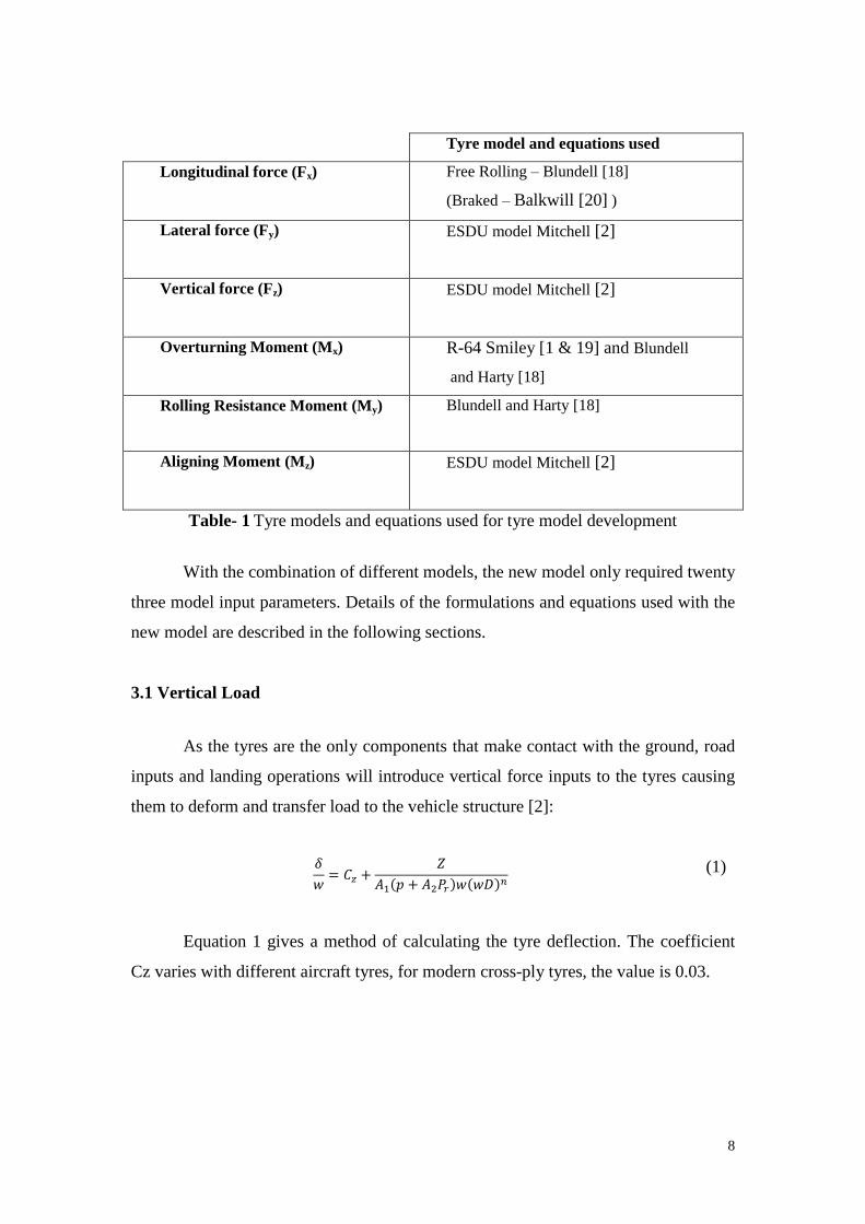
8

Tyre model and equations used

Longitudinal force (Fx) Free Rolling – Blundell [18]

(Braked – Balkwill [20] )

Lateral force (Fy) ESDU model Mitchell [2]

Vertical force (Fz) ESDU model Mitchell [2]

Overturning Moment (Mx) R-64 Smiley [1 & 19] and Blundell

and Harty [18]

Rolling Resistance Moment (My) Blundell and Harty [18]

Aligning Moment (Mz) ESDU model Mitchell [2]

Table- 1 Tyre models and equations used for tyre model development

With the combination of different models, the new model only required twenty

three model input parameters. Details of the formulations and equations used with the

new model are described in the following sections.

3.1 Vertical Load

As the tyres are the only components that make contact with the ground, road

inputs and landing operations will introduce vertical force inputs to the tyres causing

them to deform and transfer load to the vehicle structure [2]:

𝛿

𝑤= 𝐶𝑧 +

𝑍

𝐴1(𝑝 + 𝐴2𝑃𝑟)𝑤(𝑤𝐷)𝑛

(1)

Equation 1 gives a method of calculating the tyre deflection. The coefficient

Cz varies with different aircraft tyres, for modern cross-ply tyres, the value is 0.03.

9

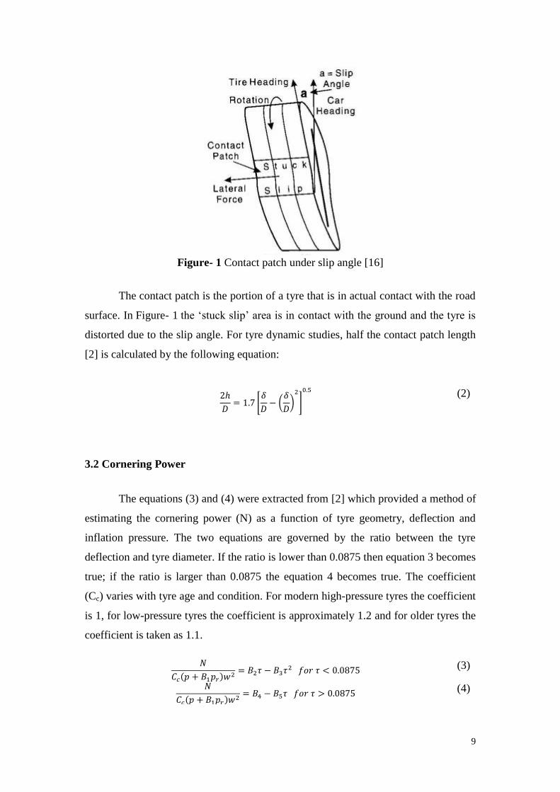
Figure- 1 Contact patch under slip angle [16]

The contact patch is the portion of a tyre that is in actual contact with the road

surface. In Figure- 1 the ‘stuck slip’ area is in contact with the ground and the tyre is

distorted due to the slip angle. For tyre dynamic studies, half the contact patch length

[2] is calculated by the following equation:

2ℎ

𝐷= 1.7 [

𝛿

𝐷− (

𝛿

𝐷)

2

]

0.5

(2)

3.2 Cornering Power

The equations (3) and (4) were extracted from [2] which provided a method of

estimating the cornering power (N) as a function of tyre geometry, deflection and

inflation pressure. The two equations are governed by the ratio between the tyre

deflection and tyre diameter. If the ratio is lower than 0.0875 then equation 3 becomes

true; if the ratio is larger than 0.0875 the equation 4 becomes true. The coefficient

(Cc) varies with tyre age and condition. For modern high-pressure tyres the coefficient

is 1, for low-pressure tyres the coefficient is approximately 1.2 and for older tyres the

coefficient is taken as 1.1.

𝑁

𝐶𝑐(𝑝 + 𝐵1𝑝𝑟)𝑤2= 𝐵2𝜏 − 𝐵3𝜏2 𝑓𝑜𝑟 𝜏 < 0.0875

(3)

𝑁

𝐶𝑐(𝑝 + 𝐵1𝑝𝑟)𝑤2= 𝐵4 − 𝐵5𝜏 𝑓𝑜𝑟 𝜏 > 0.0875

(4)

10

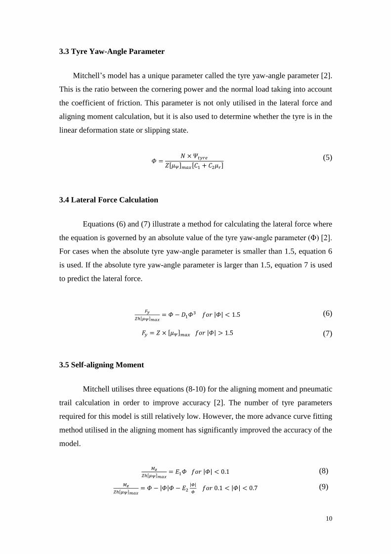
3.3 Tyre Yaw-Angle Parameter

Mitchell’s model has a unique parameter called the tyre yaw-angle parameter [2].

This is the ratio between the cornering power and the normal load taking into account

the coefficient of friction. This parameter is not only utilised in the lateral force and

aligning moment calculation, but it is also used to determine whether the tyre is in the

linear deformation state or slipping state.

𝛷 =𝑁 × 𝛹𝑡𝑦𝑟𝑒

𝑍[𝜇𝛹]𝑚𝑎𝑥[𝐶1 + 𝐶2𝜇𝑟]

(5)

3.4 Lateral Force Calculation

Equations (6) and (7) illustrate a method for calculating the lateral force where

the equation is governed by an absolute value of the tyre yaw-angle parameter (Φ) [2].

For cases when the absolute tyre yaw-angle parameter is smaller than 1.5, equation 6

is used. If the absolute tyre yaw-angle parameter is larger than 1.5, equation 7 is used

to predict the lateral force.

𝐹𝑦

𝑍ℎ[𝜇𝛹]𝑚𝑎𝑥= 𝛷 − 𝐷1𝛷3 𝑓𝑜𝑟 |𝛷| < 1.5

(6)

𝐹𝑦 = 𝑍 × [𝜇𝛹]𝑚𝑎𝑥 𝑓𝑜𝑟 |𝛷| > 1.5 (7)

3.5 Self-aligning Moment

Mitchell utilises three equations (8-10) for the aligning moment and pneumatic

trail calculation in order to improve accuracy [2]. The number of tyre parameters

required for this model is still relatively low. However, the more advance curve fitting

method utilised in the aligning moment has significantly improved the accuracy of the

model.

𝑀𝑧

𝑍ℎ[𝜇𝛹]𝑚𝑎𝑥= 𝐸1𝛷 𝑓𝑜𝑟 |𝛷| < 0.1 (8)

𝑀𝑧

𝑍ℎ[𝜇𝛹]𝑚𝑎𝑥= 𝛷 − |𝛷|𝛷 − 𝐸2

|𝛷|

𝛷 𝑓𝑜𝑟 0.1 < |𝛷| < 0.7 (9)

11

𝑀𝑧

𝑍ℎ[𝜇𝛹]𝑚𝑎𝑥= 𝐸3

|𝛷|

𝛷− 𝐸4𝛷 𝑓𝑜𝑟 0.7 < |𝛷| < 1.2 (10)

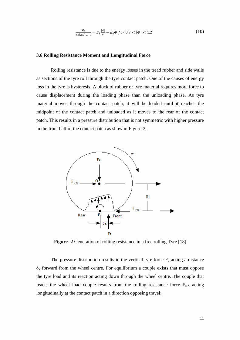
3.6 Rolling Resistance Moment and Longitudinal Force

Rolling resistance is due to the energy losses in the tread rubber and side walls

as sections of the tyre roll through the tyre contact patch. One of the causes of energy

loss in the tyre is hysteresis. A block of rubber or tyre material requires more force to

cause displacement during the loading phase than the unloading phase. As tyre

material moves through the contact patch, it will be loaded until it reaches the

midpoint of the contact patch and unloaded as it moves to the rear of the contact

patch. This results in a pressure distribution that is not symmetric with higher pressure

in the front half of the contact patch as show in Figure-2.

Figure- 2 Generation of rolling resistance in a free rolling Tyre [18]

The pressure distribution results in the vertical tyre force Fz acting a distance

δx forward from the wheel centre. For equilibrium a couple exists that must oppose

the tyre load and its reaction acting down through the wheel centre. The couple that

reacts the wheel load couple results from the rolling resistance force FRX acting

longitudinally at the contact patch in a direction opposing travel:

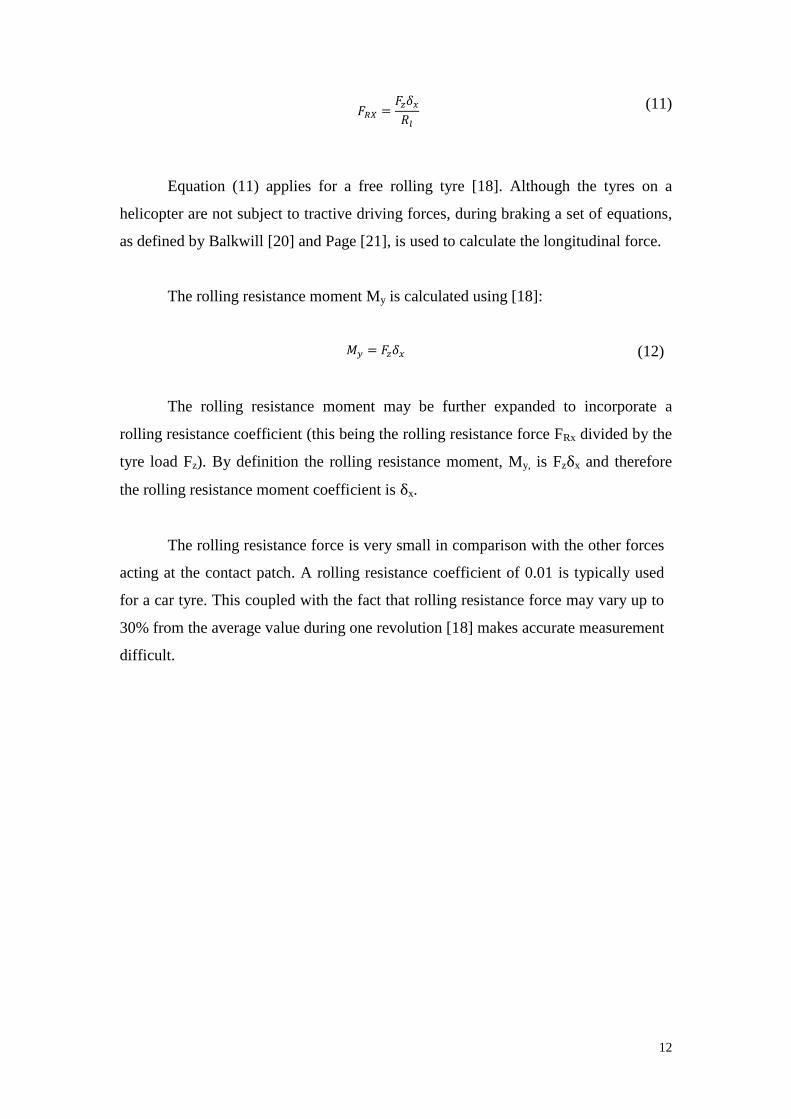
12

𝐹𝑅𝑋 =𝐹𝑧𝛿𝑥

𝑅𝑙

(11)

Equation (11) applies for a free rolling tyre [18]. Although the tyres on a

helicopter are not subject to tractive driving forces, during braking a set of equations,

as defined by Balkwill [20] and Page [21], is used to calculate the longitudinal force.

The rolling resistance moment My is calculated using [18]:

𝑀𝑦 = 𝐹𝑧𝛿𝑥 (12)

The rolling resistance moment may be further expanded to incorporate a

rolling resistance coefficient (this being the rolling resistance force FRx divided by the

tyre load Fz). By definition the rolling resistance moment, My, is Fzδx and therefore

the rolling resistance moment coefficient is δx.

The rolling resistance force is very small in comparison with the other forces

acting at the contact patch. A rolling resistance coefficient of 0.01 is typically used

for a car tyre. This coupled with the fact that rolling resistance force may vary up to

30% from the average value during one revolution [18] makes accurate measurement

difficult.

13

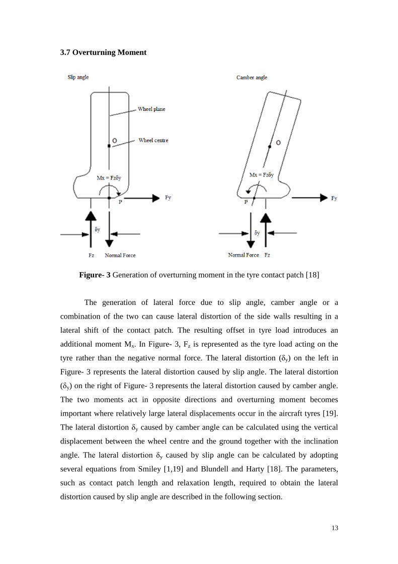
3.7 Overturning Moment

Figure- 3 Generation of overturning moment in the tyre contact patch [18]

The generation of lateral force due to slip angle, camber angle or a

combination of the two can cause lateral distortion of the side walls resulting in a

lateral shift of the contact patch. The resulting offset in tyre load introduces an

additional moment Mx. In Figure- 3, Fz is represented as the tyre load acting on the

tyre rather than the negative normal force. The lateral distortion (δy) on the left in

Figure- 3 represents the lateral distortion caused by slip angle. The lateral distortion

(δy) on the right of Figure- 3 represents the lateral distortion caused by camber angle.

The two moments act in opposite directions and overturning moment becomes

important where relatively large lateral displacements occur in the aircraft tyres [19].

The lateral distortion δy caused by camber angle can be calculated using the vertical

displacement between the wheel centre and the ground together with the inclination

angle. The lateral distortion δy caused by slip angle can be calculated by adopting

several equations from Smiley [1,19] and Blundell and Harty [18]. The parameters,

such as contact patch length and relaxation length, required to obtain the lateral

distortion caused by slip angle are described in the following section.

14

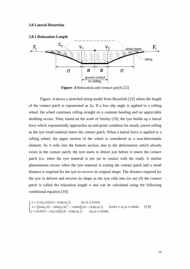
3.8 Lateral Distortion

3.8.1 Relaxation Length

Figure- 4 Relaxation and contact patch [22]

Figure- 4 shows a stretched string model from Besselink [22] where the length

of the contact patch is represented as 2a. If a low slip angle is applied to a rolling

wheel, the wheel continues rolling straight on a constant heading and no appreciable

skidding occurs. Then, based on the work of Smiley [19], the tyre builds up a lateral

force which exponentially approaches an end-point condition for steady yawed rolling

as the tyre tread material enters the contact patch. When a lateral force is applied to a

rolling wheel, the upper section of the wheel is considered as a non-deformable

element. As it rolls into the bottom section, due to the deformation which already

exists in the contact patch, the tyre starts to distort just before it enters the contact

patch (i.e. when the tyre material is not yet in contact with the road). A similar

phenomenon occurs when the tyre material is exiting the contact patch and a small

distance is required for the tyre to recover its original shape. The distance required for

the tyre to deform and recover its shape as the tyre rolls into (or out of) the contact

patch is called the relaxation length σ and can be calculated using the following

conditional equation [19]:

{

𝜎 = (11𝛿0 𝑑⁄ )(2.8 − (0.8𝑝 𝑝𝑟⁄ )) (𝛿0 𝑑 ≤ 0.053)⁄

𝜎 = [(64𝛿0 𝑑⁄ ) − 500(𝛿0 𝑑)⁄ 2− 1.4045](2.8 − (0.8𝑝 𝑝𝑟⁄ ))

𝜎 = [0.9075 − (4𝛿0 𝑑⁄ )](2.8 − (0.8𝑝 𝑝𝑟⁄ )) (𝛿0 𝑑 ≥ 0.068)⁄

(0.053 ≤ 𝛿0 𝑑⁄ ≤ 0.068) (13)

15

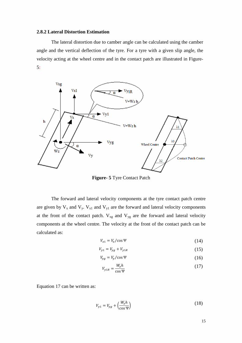
2.8.2 Lateral Distortion Estimation

The lateral distortion due to camber angle can be calculated using the camber

angle and the vertical deflection of the tyre. For a tyre with a given slip angle, the

velocity acting at the wheel centre and in the contact patch are illustrated in Figure-

5:

Figure- 5 Tyre Contact Patch

The forward and lateral velocity components at the tyre contact patch centre

are given by Vx and Vy. Vx1 and Vy1 are the forward and lateral velocity components

at the front of the contact patch. Vxg and Vyg are the forward and lateral velocity

components at the wheel centre. The velocity at the front of the contact patch can be

calculated as:

𝑉𝑥1 = 𝑉𝑥 cos Ψ⁄ (14)

𝑉𝑦1 = 𝑉𝑦𝑔 + 𝑉𝑦1𝑅 (15)

𝑉𝑦𝑔 = 𝑉𝑦 cos Ψ⁄ (16)

𝑉𝑦1𝑅 =𝑊𝑧ℎ

cos Ψ

(17)

Equation 17 can be written as:

𝑉𝑦1 = 𝑉𝑦𝑔 + (𝑊𝑧ℎ

cos Ψ)

(18)

16

The lateral distortion at the front of the contact patch can be calculated using the

following equation:

𝜆1 = 𝜎Ψ − 𝜎(𝑉𝑦1 𝑉𝑥1⁄ ) (19)

For a time dependant solution the current solution step should include the same effect

as the previous step. If K is assumed to be the current step and T the time of the

simulation and a simulation is run, for example, for 10 seconds with 100 steps (when

K is 1), the time of a simulation should be at least 0.1s. Also if J is the previous step

then it can be seen that J = K – 1.

For look back distance:

𝑑𝑒𝑙𝑡0 = 𝜎 𝑉𝑥⁄ (20)

𝑇𝑏𝑎𝑐𝑘 = 𝑇𝑖𝑚𝑒 − 𝑇𝑖𝑚𝑒(𝐽) (21)

If Tback is greater than delt0:

𝐺𝑟𝑎𝑑0 = [𝜆1(𝐾) − 𝜆1(𝐽)] [𝑇𝑖𝑚𝑒(𝐾) − 𝑇𝑖𝑚𝑒(𝐽)]⁄ (22)

𝜆0 = 𝜆1(𝐾) + 𝐺𝑟𝑎𝑑0 ∗ (𝑇𝑏𝑎𝑐𝑘 − 𝑑𝑒𝑙𝑡0) (23)

If K = 1 and Tback is smaller than delt0, then

𝜆0 = 𝜆1 (24)

For a look back distance H:

𝑑𝑒𝑙𝑡2 = 2𝜎 𝑉𝑥⁄ (25)

If Tback is greater than delt2:

𝐺𝑟𝑎𝑑2 = [𝜆1(𝐾) − 𝜆1(𝐽)] [𝑇𝑖𝑚𝑒(𝐾) − 𝑇𝑖𝑚𝑒(𝐽)]⁄ (26)

𝜆2 = 𝜆1(𝐾) + 𝐺𝑟𝑎𝑑2 ∗ (𝑇𝑏𝑎𝑐𝑘 − 𝑑𝑒𝑙𝑡0) (27)

17

If K = 1 and Tback is smaller than delt2, then

𝜆0 = 𝜆2 (28)

In summary the parameters for the new aircraft tyre model are listed in Table- 2:

Table- 2

A1 Tyre pressure coefficient for vertical force calculation

A2 Rated tyre pressure coefficient for vertical force calculation

B1 Rated tyre pressure coefficient for cornering power calculation

B2,B3 Cornering power coefficient for τ below 0.0875

B4,B5 Cornering power coefficient for τ above 0.0875

C1, C2 Yaw angle parameter friction coefficient

D1 Lateral force coefficient for linear deformation phase

E1 Aligning moment coefficient for linear deformation phase

E2 Aligning moment coefficient for transition phase

E3 Aligning moment coefficient for slipping phase

Table- 2 Table of Coefficient Description

4. Co-simulation and Building a Tyre Subroutine in Matlab

The MSC.ADAMS software is a general purpose industry standard multi-body

simulation tool where programming tyre model equations directly into ADAMS is

based on a code compiling format. This is not always a convenient method for tyre

model development if the tyre model needs to be exported to other simulation

environments. Developing a tyre subroutine is an effective solution to counter this

problem where the tyre subroutine file (.dll) contains all of the constant values,

equations and the necessary variables for calculating the tyre model outputs [23].

During simulation information such as slip angel and camber angle is passed to the

model subroutine file simultaneously so that it can calculate the tyre force and

moment outputs for the next time step and pass these back to the vehicle or aircraft

model. The software chosen for the tyre subroutine development for this investigation

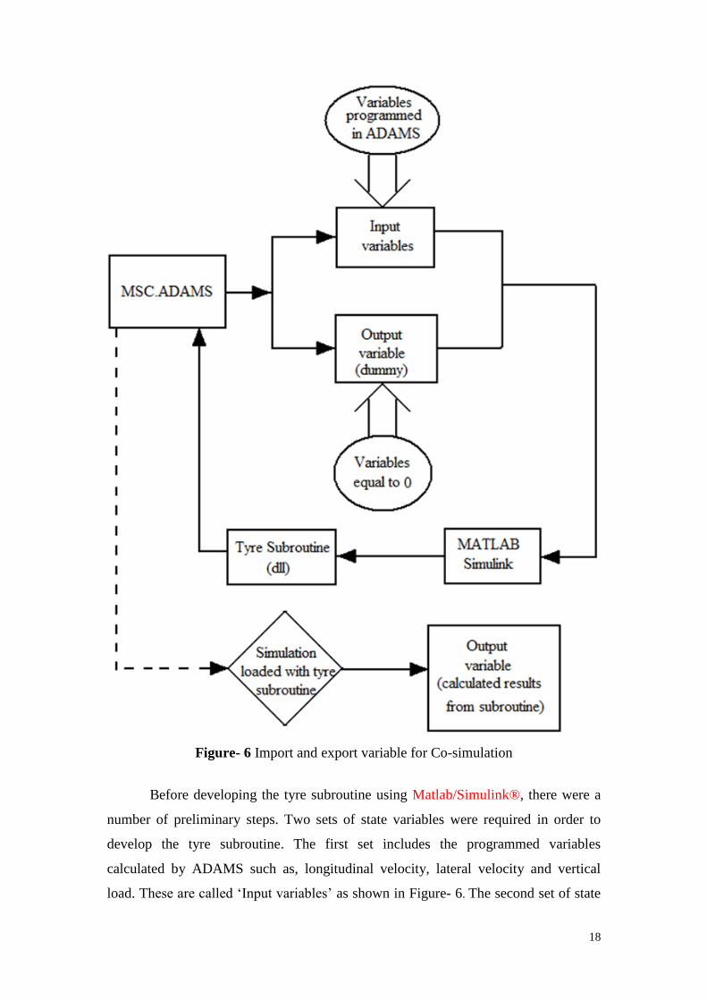
was Matlab/Simulink®. The process of co-simulation is illustrated in Figure- 6.

18

Figure- 6 Import and export variable for Co-simulation

Before developing the tyre subroutine using Matlab/Simulink®, there were a

number of preliminary steps. Two sets of state variables were required in order to

develop the tyre subroutine. The first set includes the programmed variables

calculated by ADAMS such as, longitudinal velocity, lateral velocity and vertical

load. These are called ‘Input variables’ as shown in Figure- 6. The second set of state

19

variables are dummy variables, i.e. variables set equal to zero. These dummy

variables need to be setup in relation to the desire outputs calculated by the tyre

subroutine such as longitudinal force, lateral force and aligning moment. After setting

the ‘control plan export’, ADAMS will generate a file that is compatible with

Matlab®. Matlab/Simulink®. Unlike other software, instead of using direct

programming, Matlab/Simulink® uses block and flow diagrams to represent

mathematical calculations.

After the programme in Matlab/Simulink® was completed, the ‘real time

workshop’ function was used to create a subroutine file (.dll) as shown in Figure- 6.

The tyre model subroutine was then imported back and integrated with the chosen

multi-body simulation model file. Further information on how to setup the ‘real time

workshop’ can be found in [24].

5. Tyre Modelling and Simulation

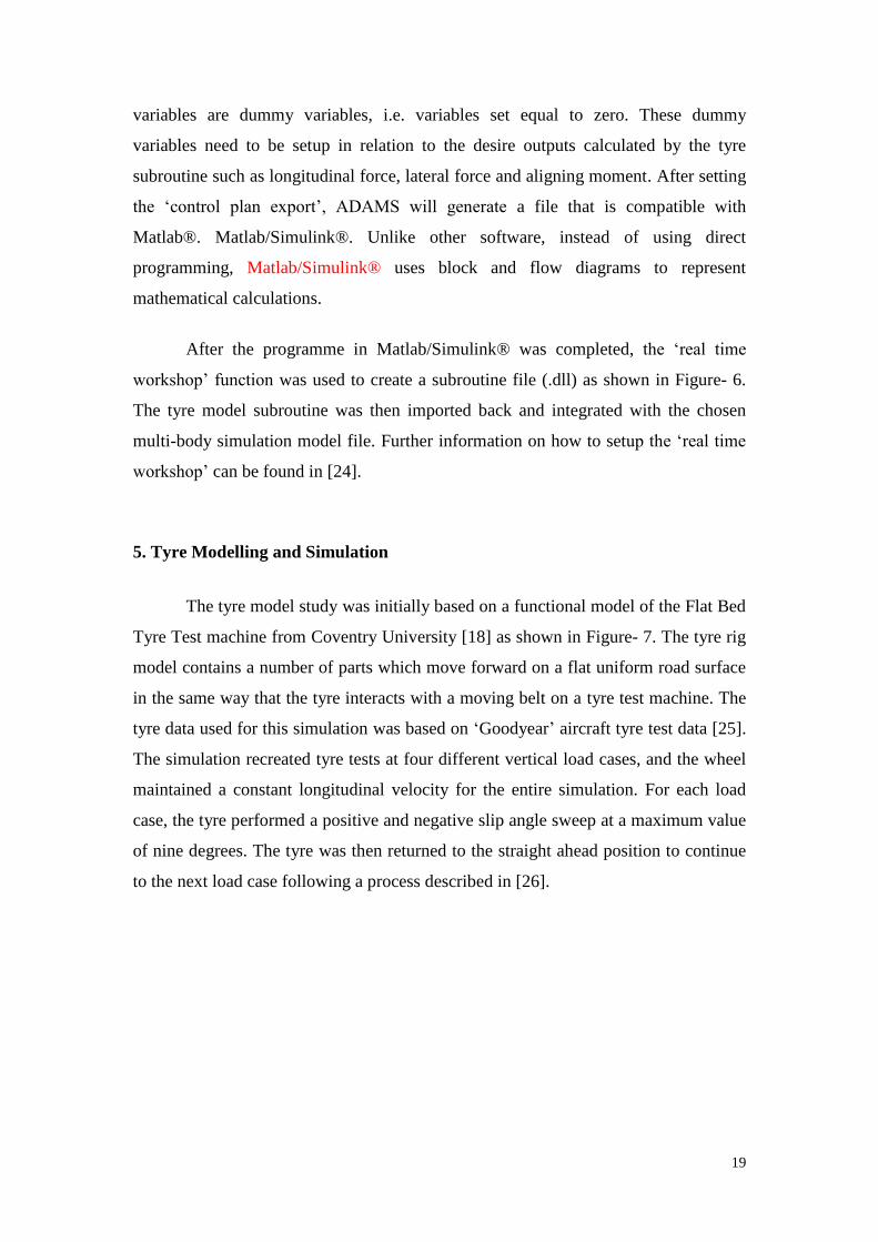
The tyre model study was initially based on a functional model of the Flat Bed

Tyre Test machine from Coventry University [18] as shown in Figure- 7. The tyre rig

model contains a number of parts which move forward on a flat uniform road surface

in the same way that the tyre interacts with a moving belt on a tyre test machine. The

tyre data used for this simulation was based on ‘Goodyear’ aircraft tyre test data [25].

The simulation recreated tyre tests at four different vertical load cases, and the wheel

maintained a constant longitudinal velocity for the entire simulation. For each load

case, the tyre performed a positive and negative slip angle sweep at a maximum value

of nine degrees. The tyre was then returned to the straight ahead position to continue

to the next load case following a process described in [26].

20

Figure- 7 Test Rig Model [18]

6. Simulated Test Rig Results

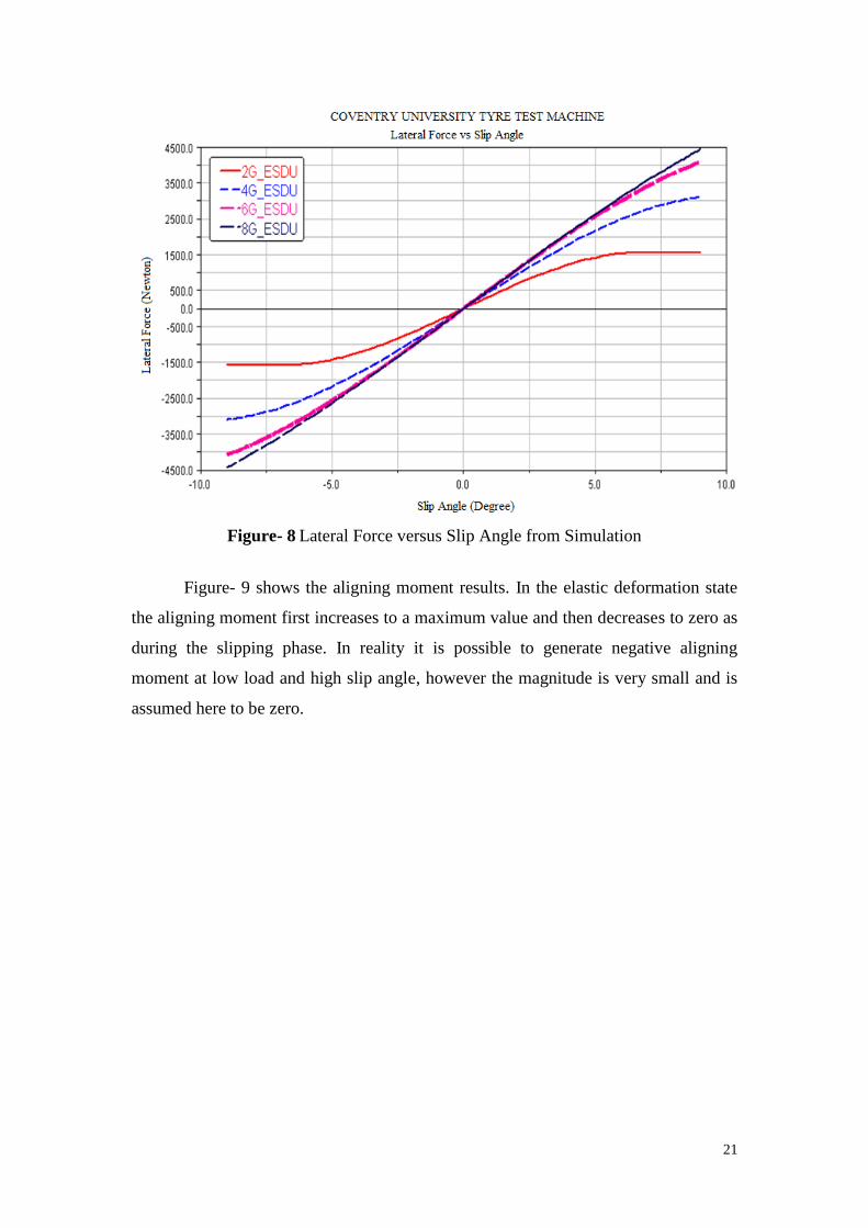
Figure- 8 shows the simulation results for slip angle versus lateral force at

various tyre loads. For loads corresponding to 4G, 6G and 8G the lateral force

increases linearly as the slip angle is varied between plus and minus nine degrees.

This shows that the tyre is undergoes elastic deformation in this region. From the 2G

test, the lateral force first varies linearly as the slip angle increases. As the slip angle

increases beyond six degrees, the lateral force stops increasing and becomes constant.

This effect shows that the energy generated from slip angle has passed beyond that

which the tyre can sustain which results in the tyre slipping. The slip angle at which

the tyre transfers from an elastic deformation state to a slipping state is also known as

the critical slip angle. By plotting all four load cases on the same graph, it can be seen

that the vertical force does not only influence the lateral force but also the critical slip

angle (the point of maximum lateral force). Therefore at higher vertical loads, the tyre

will experience a larger range for the elastic deformation state.

21

Figure- 8 Lateral Force versus Slip Angle from Simulation

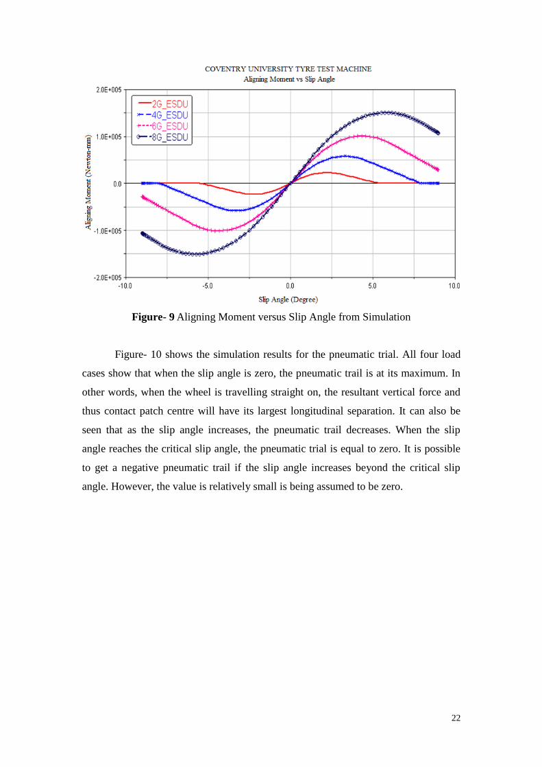
Figure- 9 shows the aligning moment results. In the elastic deformation state

the aligning moment first increases to a maximum value and then decreases to zero as

during the slipping phase. In reality it is possible to generate negative aligning

moment at low load and high slip angle, however the magnitude is very small and is

assumed here to be zero.

22

Figure- 9 Aligning Moment versus Slip Angle from Simulation

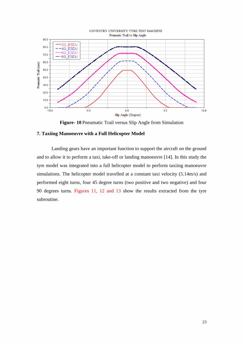
Figure- 10 shows the simulation results for the pneumatic trial. All four load

cases show that when the slip angle is zero, the pneumatic trail is at its maximum. In

other words, when the wheel is travelling straight on, the resultant vertical force and

thus contact patch centre will have its largest longitudinal separation. It can also be

seen that as the slip angle increases, the pneumatic trail decreases. When the slip

angle reaches the critical slip angle, the pneumatic trial is equal to zero. It is possible

to get a negative pneumatic trail if the slip angle increases beyond the critical slip

angle. However, the value is relatively small is being assumed to be zero.

23

Figure- 10 Pneumatic Trail versus Slip Angle from Simulation

7. Taxiing Manoeuvre with a Full Helicopter Model

Landing gears have an important function to support the aircraft on the ground

and to allow it to perform a taxi, take-off or landing manoeuvre [14]. In this study the

tyre model was integrated into a full helicopter model to perform taxiing manoeuvre

simulations. The helicopter model travelled at a constant taxi velocity (5.14m/s) and

performed eight turns, four 45 degree turns (two positive and two negative) and four

90 degrees turns. Figures 11, 12 and 13 show the results extracted from the tyre

subroutine.

24

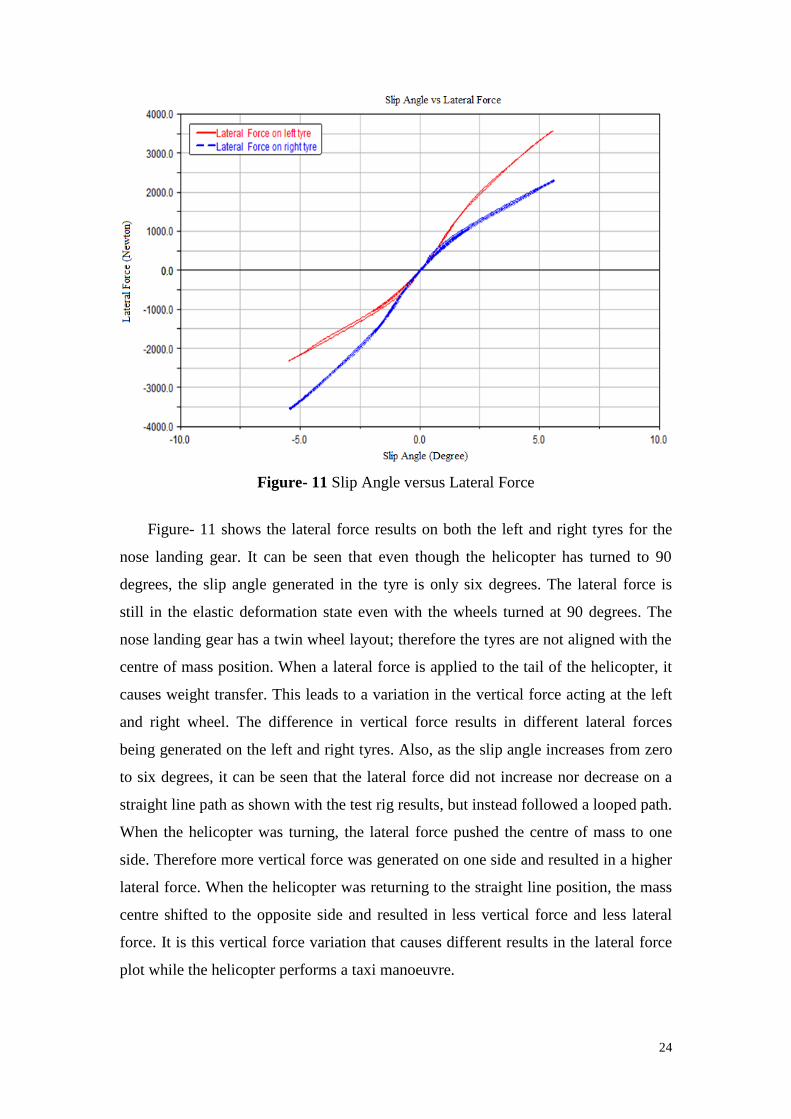
Figure- 11 Slip Angle versus Lateral Force

Figure- 11 shows the lateral force results on both the left and right tyres for the

nose landing gear. It can be seen that even though the helicopter has turned to 90

degrees, the slip angle generated in the tyre is only six degrees. The lateral force is

still in the elastic deformation state even with the wheels turned at 90 degrees. The

nose landing gear has a twin wheel layout; therefore the tyres are not aligned with the

centre of mass position. When a lateral force is applied to the tail of the helicopter, it

causes weight transfer. This leads to a variation in the vertical force acting at the left

and right wheel. The difference in vertical force results in different lateral forces

being generated on the left and right tyres. Also, as the slip angle increases from zero

to six degrees, it can be seen that the lateral force did not increase nor decrease on a

straight line path as shown with the test rig results, but instead followed a looped path.

When the helicopter was turning, the lateral force pushed the centre of mass to one

side. Therefore more vertical force was generated on one side and resulted in a higher

lateral force. When the helicopter was returning to the straight line position, the mass

centre shifted to the opposite side and resulted in less vertical force and less lateral

force. It is this vertical force variation that causes different results in the lateral force

plot while the helicopter performs a taxi manoeuvre.

25

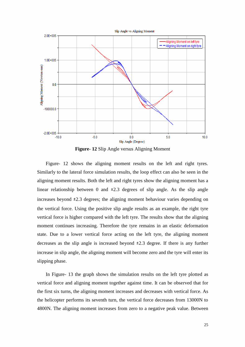
Figure- 12 Slip Angle versus Aligning Moment

Figure- 12 shows the aligning moment results on the left and right tyres.

Similarly to the lateral force simulation results, the loop effect can also be seen in the

aligning moment results. Both the left and right tyres show the aligning moment has a

linear relationship between 0 and 2.3 degrees of slip angle. As the slip angle

increases beyond 2.3 degrees; the aligning moment behaviour varies depending on

the vertical force. Using the positive slip angle results as an example, the right tyre

vertical force is higher compared with the left tyre. The results show that the aligning

moment continues increasing. Therefore the tyre remains in an elastic deformation

state. Due to a lower vertical force acting on the left tyre, the aligning moment

decreases as the slip angle is increased beyond 2.3 degree. If there is any further

increase in slip angle, the aligning moment will become zero and the tyre will enter its

slipping phase.

In Figure- 13 the graph shows the simulation results on the left tyre plotted as

vertical force and aligning moment together against time. It can be observed that for

the first six turns, the aligning moment increases and decreases with vertical force. As

the helicopter performs its seventh turn, the vertical force decreases from 13000N to

4800N. The aligning moment increases from zero to a negative peak value. Between

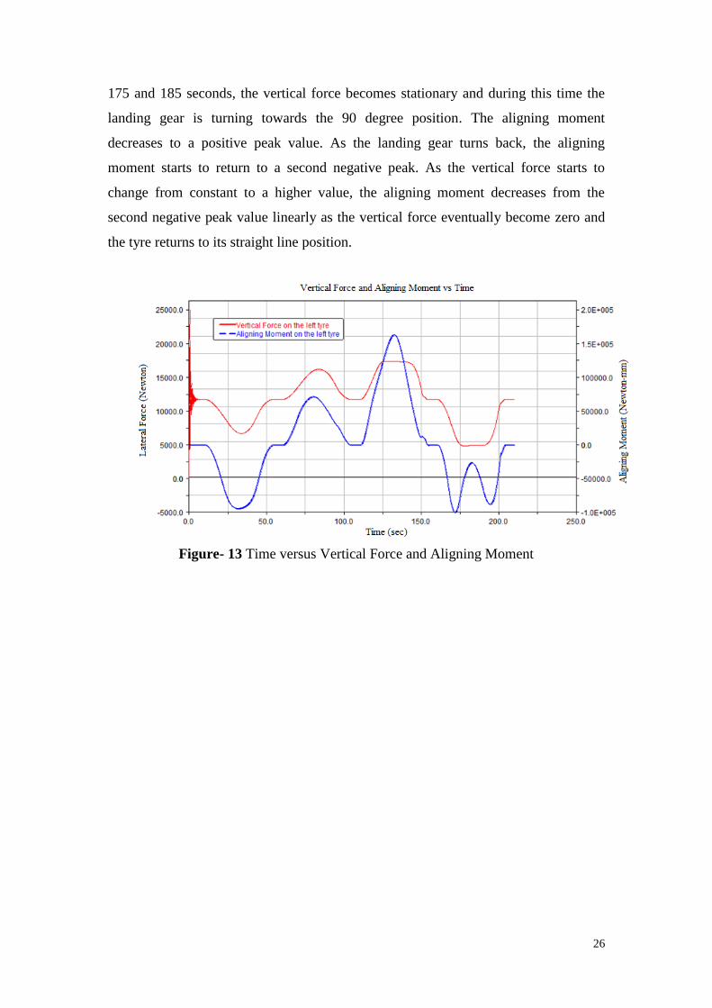
26

175 and 185 seconds, the vertical force becomes stationary and during this time the

landing gear is turning towards the 90 degree position. The aligning moment

decreases to a positive peak value. As the landing gear turns back, the aligning

moment starts to return to a second negative peak. As the vertical force starts to

change from constant to a higher value, the aligning moment decreases from the

second negative peak value linearly as the vertical force eventually become zero and

the tyre returns to its straight line position.

Figure- 13 Time versus Vertical Force and Aligning Moment

27

8. Conclusions

A unique tyre model was developed specially for helicopter ground operation

simulations. Various tyre models were reviewed to provide a basis for the

formulations in the new tyre model. Following consideration of existing available tyre

models and the with the project research aim of developing a low parameter tyre

model, the ESDU tyre model developed by Mitchell [2] was used as the model

foundation. The model was completed by adopting other equations from Blundell and

Harty [18] and the R-64 model by Smiley [1] resulting in a new model that only

requires twenty three input parameters. To make the model portable, a co-simulation

method was also utilised. The tyre model was programmed in Matlab/Simulink® and

formatted into a subroutine file. The subroutine file was then imported into

MSC.ADAMS and loaded with the multi-body helicopter model to perform different

simulations. The model was first imported to a virtual tyre test rig to validate the basic

properties of the tyre model. The tyre model was then imported to a full helicopter

model and used successfully to perform taxiing manoeuvre simulations. From the

runway manoeuvre simulation results, the tyre model showed its capability to capture

various dynamic characteristics.

The tyre model developed in this investigation has been shown to integrate the

low parameter principle whilst maintaining detailed calculations for some of the

important tyre responses. The lateral force and the aligning moment were created with

a suitable level of precision. However, the aim of this project was to replicate the

response of the lateral and longitudinal force of the tyre. This could not be achieved

due to a lack of suitable test data. If tyre test data were to become available the tyre

model could be developed further. This would significantly advance the research

already conducted and lead to improved tools for helicopter design and the simulation

of aircraft ground dynamics.

28

9. References

1. Smiley, R.F. and Horne, W.B. Mechanical properties of pneumatic tyres with

special reference to modern aircraft tyre R-64, NASA,. 1957 (USA)

2. Mitchell, D.J. Frictional and Retarding Forces on Aircraft Tyres Part IV:

Estimation of Effects of Yaw, ESDU,. 1986. 86016

3. Pacejka, H.B. Tyre and Vehicle Dynamics. 2006, 321-358 (ELSEVIER,

Netherlands, second edition).

4. Besselink, I.J.M., Schmeitz, A.J.C., and Pacejka, H.B. An Improved Magic

Formula/SWIFT Tyre Model That Can Handle Inflation Pressure Changes. 2000,

(Department of Mechanical Engineering, Eindhoven University of Technology).

5. Kiebre, R. Contribution to the Modelling of Aircraft Tyre-Road Interaction.

University De Haute-Alsace PhD thesis,. 2010. (France)

6. Mavros, G., Rahnejat, H. and King, P.D. Transient analysis of tyre friction

generation using a brush model with interconnected viscoelastic bristles. J.

Multibody Dynamics,. 2004, 219(K). 7. Gim, G. and Nikravesh, P. E. An analytical model of pneumatic tyres for

vehicle denamic simulations. Part 1: pure slips, International Journal of Vehicle

Design,. 1990, 11(6).

8. Gim, G. and Nikravesh, P. E. An analytical model of pneumatic tyres for

vehicle denamic simulations. Part 2: pure slips, International Journal of Vehicle

Design, 1991, 12(1).

9. Gim, G. and Nikravesh, P. E. An analytical model of pneumatic tyres for

vehicle denamic simulations. Part 3: pure slips, International Journal of Vehicle

Design, 1991, 12(2).

10. Wood, G. Aircraft Tyre Modelling. Coventry University PhD thesis.. 2006. (U.K.)

11. Gipser, M. FTire - Flexible Ring Tire Model. Cosin Scientific Software,. 2013.

12. YANG, X.G. Finite Element Analysis and Experimental Investigation of Tyre

Characteristics for Developing Strain-based Intelligent Tyre. Birmingham

University PhD thesis,. 2011. (U.K.)

13. Moreland, W.J. The Story of Shimmy. Journal of the Aeronautical Sciences,.

1954. 21(12).

14. Moore, D.F. The Friction of Pneumatic Tyres. 1975, 323-325 (ELSEVIER,

Amsterdam-Oxford-New York).

29

15. Grossman, D.T. F-15 nose landing gear shimmy, taxi test and correlative

analyses. SAE Technical Paper,. 1980, 801239

16. Haney, P. The Racing and high-performance tyre, 2003, (TV MOTORSPORTS

and SAE, United States of America) R-351.

17. Butts, D. and Kogan, A. Helicopter landing gear shimmy analysis. American

helicopter society international, Inc,. May 2010. (66th Annual Forum, Phoenix,

AZ, USA)

18. Blundell, M.V. and Harty, D. The Multibody systems Approach to Vehicle

Dynamics. 2004, 248~325 (ELSEVIER, UK).

19. Smiley, R.F. Correlation, Evaluation, and Extension of linearized theories for

tyre motion and wheel shimmy. NASA,. 1956.

20. Balkwill, K.J. Comprehensive method for modeling performance of aircraft type

tyres rolling or braking on runways contaminated with water, slush, snow, ice.

ESDU,. May 2005. 05011.

21. Page, A.N. Frictional and Retarding Forces on Aircraft Tyres Part IV: Estimation

of Effects of Yaw. ESDU,. 1986, 71025.

22. Besselink, I.J.M. Shimmy of aircraft main landing gear. voorzitter van het

College PhD thesis,. 2000. (Netherlands)

23. Feng, J.Z., Yu, F. and Zhao, Y.X. Design of a Bandwidth-limited Active

suspension Controller for Off-Road Vehicle Base on the Co-simulation

Technology. Journal of Shanghai Jiao Tong University,. 2004, 3(1).

24. MSC.ADAMS, Getting Started Using ADAMS/Controls. MSC.Software

Corporation, year 2004.

25. Aircraft tyre engineering GOODYEAR tyre and rubber company.

Nosewheel tyres for the Westland Helicopter. Agusta Westland Helicopter,

March 1989.

26. HEGAZY, S., H. RAHNEJAT, and K. HUSSAIN. Dynamic tyre testing for

vehicle handling studies. Multibody Dynamics: Monitoring and Simulation

Techniques II,. 2000, 135.

30

List of Figures

Figure- 1 Contact patch under slip angle [16] ......................................................... 9

Figure- 2 Generation of Rolling Resistance in a Free Rolling Tyre [18] .............. 11

Figure- 3 Generation of overturning moment in the tyre contact patch [18] ........ 13

Figure- 4 Relaxation and contact patch [22] ......................................................... 14

Figure- 5 Tyre Contact Patch ................................................................................ 15

Figure- 6 Import and export variable for Co-simulation ....................................... 18

Figure- 7 Test Rig Model [18] .............................................................................. 20

Figure- 8 Lateral Force versus Slip Angle from Simulation ................................. 21

Figure- 9 Aligning Moment versus Slip Angle from Simulation ......................... 22

Figure- 10 Pneumatic Trail versus Slip Angle from Simulation ........................... 23

Figure- 11 Slip Angle versus Lateral Force .......................................................... 24

Figure- 12 Slip Angle versus Aligning Moment ................................................... 25

Figure- 13 Time versus Vertical Force and Aligning Moment ............................. 26

Table- 1 Tyre models and equations used for tyre model development ................. 8

Table- 2 Table of Coefficient Description ............................................................ 17