U. Rascher et al. CEFLES2: the remote sensing component …pubman.mpdl.mpg.de/pubman/item/escidoc:1692840/... · BGD 6, 2217–2266, 2009 CEFLES2 U. Rascher et al. Title Page Abstract

BGD6, 2217–2266, 2009

CEFLES2

U. Rascher et al.

Title Page

Abstract Introduction

Conclusions References

Tables Figures

J I

J I

Back Close

Full Screen / Esc

Printer-friendly Version

Interactive Discussion

Biogeosciences Discuss., 6, 2217–2266, 2009www.biogeosciences-discuss.net/6/2217/2009/© Author(s) 2009. This work is distributed underthe Creative Commons Attribution 3.0 License.

BiogeosciencesDiscussions

Biogeosciences Discussions is the access reviewed discussion forum of Biogeosciences

CEFLES2: the remote sensing componentto quantify photosynthetic efficiency fromthe leaf to the region by measuringsun-induced fluorescence in the oxygenabsorption bandsU. Rascher1, G. Agati2, L. Alonso3, G. Cecchi2, S. Champagne4, R. Colombo5,A. Damm6, F. Daumard4, E. de Miguel7, G. Fernandez3, B. Franch8, J. Franke9,C. Gerbig10, B. Gioli11, J. A. Gomez7, Y. Goulas4, L. Guanter12,O. Gutierrez-de-la-Camara7, K. Hamdi1, P. Hostert6, M. Jimenez7,M. Kosvancova13, D. Lognoli2, M. Meroni5, F. Miglietta11, A. Moersch1,J. Moreno3, I. Moya4, B. Neininger14, A. Okujeni6, A. Ounis4, L. Palombi2,V. Raimondi2, A. Schickling15, J. A. Sobrino8, M. Stellmes16, G. Toci2,P. Toscano11, T. Udelhoven17, S. van der Linden6, and A. Zaldei11

1Institute of Chemistry and Dynamics of the Geosphere, ICG-3: Phytosphere,Forschungszentrum Julich, Leo-Brandt-Str., 52425 Julich, Germany

2217

http://www.biogeosciences-discuss.net

http://www.biogeosciences-discuss.net/6/2217/2009/bgd-6-2217-2009-print.pdf

http://www.biogeosciences-discuss.net/6/2217/2009/bgd-6-2217-2009-discussion.html

http://creativecommons.org/licenses/by/3.0/

BGD6, 2217–2266, 2009

CEFLES2

U. Rascher et al.

Title Page



Tables Figures

J I

J I

Back Close

Full Screen / Esc



2IFAC-CNR, Istituto di Fisica Applicata “Nello Carrara”, Consiglio Nazionale delle Ricerche, viaMadonna del Piano 10, 50019, Sesto F.no, Firenze, Italy3Department of Earth Physics and Thermodynamics, University of Valencia, Dr Moliner, 50,46100 Burjassot – Valencia, Spain4Lab. de Meteorologie Dynamique, CNRS, Ecole Polytechnique, 91128 Palaiseau, France5Remote Sensing of Environmental Dynamics Lab., DISAT, University of Milan-Bicocca, Piazzadella Scienza 1, 20126 Milano, Italy6Geomatics Lab, Humboldt-Universitat zu Berlin, Unter den Linden 6, 10099 Berlin, Germany7Remote Sensing Laboratory, Instituto Nacional de Tecnica Aeroespacial, Carr. de Ajalvir, km4, 28850 Torrejon de Ardoz, Madrid, Spain8Global Change Unit, Imaging Processing Laboratory, University of Valencia, Pol. “La Coma”,s/n. 46980 Paterna-Valencia, Spain9Center for Remote Sensing of Land Surfaces (ZFL), University of Bonn, Walter-Flex-Strasse3, 53113 Bonn, Germany10Max Planck Institute for Biogeochemistry, Hans Knoell Str. 10, 07745 Jena, Germany11IBIMET-CNR, Instituto di Biometeorologia, Consiglia Nazionale delle Ricerche, Via G.Caproni 8, 50145 Firenze, Italy12Helmholtz Centre Potsdam, GFZ German Research Centre for Geosciences, Department 1– Geodesy and Remote Sensing, Telegrafenberg, 14473 Potsdam, Germany13Laboratory of Plants Ecological Physiology, Division of Ecosystem Processes, Institute ofSystems Biology and Ecology, Porıcı 3b, 60300 Brno, Czech Republic14Metair AG, Flugplatz, 8915 Hausen am Albis, Switzerland15Institute for Geophysics and Meteorology, University of Cologne, Kerpener Str. 13, 50937Cologne, Germany16Remote Sensing Department, Trier University, 54286 Trier, Germany17CRP-Gabriel Lippmann, Departement “Environnement et Agro-biotechnologies”, GeomaticPlatform, 41, rue du Brill, 4422 Belvaux, Luxembourg

2218





BGD6, 2217–2266, 2009

CEFLES2

U. Rascher et al.

Title Page



Tables Figures

J I

J I

Back Close

Full Screen / Esc



Received: 23 December 2008 – Accepted: 8 January 2009 – Published: 24 February 2009

Correspondence to: U. Rascher ([email protected])

Published by Copernicus Publications on behalf of the European Geosciences Union.

2219





BGD6, 2217–2266, 2009

CEFLES2

U. Rascher et al.

Title Page



Tables Figures

J I

J I

Back Close

Full Screen / Esc



Abstract

The CEFLES2 campaign during the Carbo Europe Regional Experiment Strategy wasdesigned to provide simultaneous airborne measurements of solar induced fluores-cence and CO2 fluxes. It was combined with extensive ground-based quantification ofleaf- and canopy-level processes in support of ESA’s Candidate Earth Explorer Mission5

of the “Fluorescence Explorer” (FLEX). The aim of this campaign was to test if fluores-cence signal detected from an airborne platform can be used to improve estimatesof plant mediated exchange on the mesoscale. Canopy fluorescence was quantifiedfrom four airborne platforms using a combination of novel sensors: (i) the prototypeairborne sensor AirFLEX quantified fluorescence in the oxygen A and B bands, (ii)10

a hyperspectral spectrometer (ASD) measured reflectance along transects during 12day courses, (iii) spatially high resolution georeferenced hyperspectral data cubes con-taining the whole optical spectrum and the thermal region were gathered with an AHSsensor, and (iv) the first employment of the high performance imaging spectrometer HY-PER delivered spatially explicit and multi-temporal transects across the whole region.15

During three measurement periods in April, June and September 2007 structural, func-tional and radiometric characteristics of more than 20 different vegetation types in theLes Landes region, Southwest France, were extensively characterized on the ground.The campaign concept focussed especially on quantifying plant mediated exchangeprocesses (photosynthetic electron transport, CO2 uptake, evapotranspiration) and flu-20

orescence emission. The comparison between passive sun-induced fluorescence andactive laser-induced fluorescence was performed on a corn canopy in the daily cy-cle and under desiccation stress. Both techniques show good agreement in detectingstress induced fluorescence change at the 760 nm band. On the large scale, airborneand ground-level measurements of fluorescence were compared on several vegetation25

types supporting the scaling of this novel remote sensing signal. The multi-scale designof the four airborne radiometric measurements along with extensive ground activitiesfosters a nested approach to quantify photosynthetic efficiency and gross primary pro-

2220





BGD6, 2217–2266, 2009

CEFLES2

U. Rascher et al.

Title Page



Tables Figures

J I

J I

Back Close

Full Screen / Esc



ductivity (GPP) from passive fluorescence.

1 Introduction

Photosynthesis harvests light from a variable stream of solar photons and converts thisenergy to carbohydrates that fuel all plant processes and ultimately life on Earth. Theefficiency of photosynthetic electron transport and carbon fixation is highly regulated,5

depending on plant species and environmental constrains (Rascher and Nedbal, 2006;Schurr et al., 2006). Quantum efficiency of photosystem II (PSII) depends primarily onlight intensity and varies between 0.83 at leaves of dark adapted higher plants to closeto zero at high light intensities (Rascher et al., 2000). Plants have evolved a varietyof photochemical and non-photochemical regulation mechanisms that are either con-10

stitutively active or are activated on demand to optimise the distribution of energy forphotosynthesis and to avoid damage because of over-energetisation of metabolism(refer to Schulze and Caldwell, 1995, for a comprehensive summary). Thus, plant pho-tosynthesis is dynamically regulated adapting to environmental conditions and beingaffected by the ecological plasticity of each species (Turner et al., 2003b; Schurr et al.,15

2006).Remote sensing offers the unique possibility to derive spatially explicit information on

vegetation status at local, regional or landscape scale (Goetz and Prince, 1999; Hilkeret al., 2008). Reflectance signals alone, however, cannot quantify photosynthetic ac-tivity and dynamics of vegetation accurately. Great benefits would be expected from20

remote sensing techniques that quantify the actual status of photosynthetic carbon fix-ation. Monteith’s (1972, 1977) mechanistic Light Use Efficiency (LUE) concept relatesthe photosynthetic capacity to LUE, describing the potential to convert absorbed radia-tion into biomass. Accordingly, Gross Primary Productivity (GPP) can be described asa function of the fraction of absorbed photosynthetic active radiation (fAPAR) and LUE25

(Turner et al., 2003a; Hilker et al., 2008). LUE is highly variable and depends on thephenological status, structure and species composition (Field et al., 1995; Goetz and

2221





BGD6, 2217–2266, 2009

CEFLES2

U. Rascher et al.

Title Page



Tables Figures

J I

J I

Back Close

Full Screen / Esc



Prince, 1999). Due to its dynamic changes, the insufficient parameterization of LUEis identified as a major source of uncertainties in modeling GPP (Hilker et al., 2008;Running et al., 2000).

Chlorophyll fluorescence analyses are among the most powerful techniques to non-destructively quantify photosynthetic efficiency and non-photochemical energy dissipa-5

tion in photosynthetically active organisms under laboratory conditions. At canopy andfield scale, chlorophyll fluorescence emission is frequently considered to be employedas a complementary, high-capacity signal on vegetation dynamics (Papageorgiou andGovindjee, 2004). Sun-induced fluorescence can be obtained from remote sensingplatforms. Several studies have shown that it is correlated with photosynthetic effi-10

ciency and thus may serve as a proxy to quantify photosynthetic efficiency (Flexas etal., 2000, 2002).

The chlorophyll fluorescence emitted by a leaf under natural sunlight is only 1–5%of the total reflected light at a specific wavelength. This makes it particularly difficult toquantitatively extract the fluorescence signal from remote sensing data. However, at15

certain wavelengths, the solar irradiance is absorbed in the solar or earth atmosphere(so-called Fraunhofer lines); thus, there is no or greatly reduced incoming radiationat the Earth’s surface in these wavelengths (Plascyk, 1975). Solar irradiance exhibitsthree main absorption bands in the red and near infrared wavelength region: the Hαline at 656.3 nm is due to hydrogen absorption in the solar atmosphere, whereas two20

bands at 687 (O2-B) and 760 nm (O2-A) are due to absorption by molecular oxygenin the terrestrial atmosphere. The O2-A and O2-B bands especially overlap with thechlorophyll fluorescence emission spectrum and, due to their widths, have the potentialto be investigated from air- and space-borne platforms. Thus, they can be used formonitoring chlorophyll fluorescence emission under daylight excitation by the method25

of the Fraunhofer lines in-filling (Plascyck, 1975).Several studies are currently under way to evaluate the accuracy with which sun-

induced fluorescence can be used to quantify photosynthetic efficiency. With this pa-per we report the concept and first results from the CEFLES2 campaign that took

2222





BGD6, 2217–2266, 2009

CEFLES2

U. Rascher et al.

Title Page



Tables Figures

J I

J I

Back Close

Full Screen / Esc



place in the context of the Carbo Europe Regional Experiment Strategy (CERES)between April and September 2007 in Southern France (see http://www.esa.int/esaLP/SEMQACHYX3F index 0.html). This campaign combined state-of-the-art re-mote sensing with extensive field-based measurements to quantify the actual status ofphotosynthetic efficiency from the level of single leaves to a regional scale. The over-5

arching goal was to better constrain and reduce uncertainties in modelling mesoscalecarbon fluxes using fluorescence as a direct input parameter.

2 The integrated concept of CEFLES2: quantifying photosynthetic efficiencyfrom leaf- to the regional scale

CEFLES2 was designed to provide extensive and spatially resolved validation of photo-10

synthesis estimates based on remote sensing fluorescence measurements that can beobtained using airborne instrumentation. Validation data were provided by extensiveground measurements of plant mediated exchange processes (photosynthetic CO2uptake, evapotranspiration and water use efficiency), fluorescence features at the leafand canopy scale, and by CarboEurope aircraft fleet that was operating during CERES15

experimental campaigns in Les Landes (France) in April and September 2007.A multitude of vegetation specific ground measurements were acquired during three

campaigns (April, June, and September 2007). These included structural parameters(leaf area index (LAI), canopy height or fractional cover (fcover), biochemical charac-terizations (chlorophyll, water and dry matter content), physiological parameters (PAM20

fluorometry, gas exchange) and standard field spectroscopy. These more traditionalmeasurements were complemented with novel set-ups aimed to quantify fluorescenceat the canopy level. As species of major interest, winter wheat was chosen in April andcorn in September. Additionally, investigations were expanded to rapeseed, grasslandand pine in April, corn, potato, sunflower and pine in June and bean, kiwi, vine and oak25

forest in September. The intensive measurement site was Marmande during the wholeCEFLES campaign. Further test sites were located in Clairac, Le Bray, Villeneuve-sur-

2223





http://www.esa.int/esaLP/SEMQACHYX3F_index_0.html



BGD6, 2217–2266, 2009

CEFLES2

U. Rascher et al.

Title Page



Tables Figures

J I

J I

Back Close

Full Screen / Esc



Lot, and Saint Laurent du Bois.

2.1 Leaf-level: quantifying photosynthesis and fluorescence

2.1.1 PAM fluorometry to derive cardinal points of photosynthesis

Efficiency of light reactions of photosynthesis were measured on the level of singleleaves using the miniaturized Fluorescence Yield Analyser (Mini-PAM) of H. Walz (Ef-5

feltrich, Germany) with a leaf clip holder described by Bilger et al. (1995) (Fig. 1a).Spot measurements of photosynthetic photon flux density (PPFD, λ=380 nm to 710 nm)were taken inside the measuring field by the micro-quantum sensor of the Mini-PAM. Effective quantum yield of PS II (∆F/F ′

m) was calculated as (F ′m−F )/F ′

m, whereF is fluorescence yield of the light adapted sample and F ′

m is the maximum light-10

adapted fluorescence yield when a saturating light pulse (800 ms duration, intensity≈4000µmol m−2 s−1) was superimposed on the prevailing environmental light levels.The apparent rate of photosynthetic electron transport (ETR) of photosystem II (PS II)was obtained as ETR=∆F/F ′

m·PPFD·0.5·α, where the factor 0.5 assumes equal exci-tation of both photosystems; the absorption factor α was derived from leaf level optical15

measurements using an integrating sphere.Light within the canopy constantly changed and showed patches of varying intensity.

Thus, leaves were exposed to rapid changes in PPFD of various duration and inten-sity, which could not be determined analytically. ∆F/F ′

m and ETR values dynamicallyadapt primarily to these changes in light intensity, but may also reflect manifold under-20

lying physiological mechanisms. Additional parameters, such as maximum apparentelectron transport rate (ETRmax) and saturating photosynthetically active radiation canbe derived from light-response curves. In general, measurements of light-responsecurves lead to a deeper insight into characteristic parameters of a plant species, whichare not related to the momentary ambient light conditions, but rather to the ontogeny of25

a leaf and to the range of physiological plasticity of a plant. In order to obtain lightresponse characteristics, about 100 randomly distributed spot measurements were

2224





BGD6, 2217–2266, 2009

CEFLES2

U. Rascher et al.

Title Page



Tables Figures

J I

J I

Back Close

Full Screen / Esc



recorded within a field and plotted over PPFD. Light dependency data plotted in suchway were mathematically fitted using single exponential functions to quantify the char-acteristic cardinal points of photosynthesis (Rascher et al., 2000).

2.1.2 Measurement of fluorescence emission spectrum

Algorithms for fluorescence retrieval from airborne data require the characterization of5

the fluorescence emission spectrum at the leaf level. They were recorded under naturalsun light conditions using a specially built spectro-fluorometer based on a HR2000+spectro-radiometer (Ocean Optics) (Fig. 1h). This instrument used solar radiation asan excitation source. Solar radiation is filtered by a short pass blue filter and focusedonto the leaf by a converging lens to compensate the attenuation of the filter.10

The spectro-radiometer was calibrated spectrally and for linearity using a standardblack body (LI-Cor 1800-02, NE, USA) and a Hg-Ar standard lamp (CAL-2000, Mi-cropack, Germany).

Measurements were performed around solar noon and during overflights in April,June and September 2007 on grass, wheat, corn and bean leaves from the different15

experimental sites. Chlorophyll content and PPFD were systematically acquired with achlorophyll-meter (SPAD-502, Minolta) and a quantum-meter.

2.1.3 Gas exchange measurements

Using the open gas-exchange system Li-6400 (Li-Cor, USA) photosynthetic charac-teristics, i.e., CO2 assimilation rate (A), stomatal conductance to water vapor (GS ),20

transpiration rate (Tr) and intercellular CO2 concentration (Ci), were recorded for ac-tual PPFD in April. In September whole light curves allowed the estimation of e.g., Aor Tr for saturating PPFD (A1800, Tr1800). Light response curves were measured us-ing the LED light source Li-6400-02B (Li-Cor, USA). The irradiances used for the lightresponse curve were 0, 80, 250, 600, 1200 and 1800µmol (photons) m−2 s−1.25

Desiccation stress was performed on four individual plants. The CO2/H2O fluxes

2225





BGD6, 2217–2266, 2009

CEFLES2

U. Rascher et al.

Title Page



Tables Figures

J I

J I

Back Close

Full Screen / Esc



were measured as an integral signal from the central parts of leaves (investigated area6 cm2) on the 4th leaves from the top. The leaves were kept inside the assimilationchamber under constant CO2 concentration (380±5µmol CO2 mol−1), air humidity andleaf temperature (following ambient conditions) during the measurement. Air flow ratethrough the assimilation chamber was maintained at 500µmol s−1.5

2.2 Canopy-level

2.2.1 Active laser induced fluorescence

Active fluorescence spectra of vegetation were recorded by using a hyperspectral Flu-orescence LIDAR (FLIDAR) imaging system (Fig. 1c). This consists mainly of a Q-switched Nd:YAG laser, a 1 m focal length Newtonian telescope and a 300 mm focal10

length spectrometer coupled to an intensified, gated 512×512 pixels CCD detector.Imaging was carried out by scanning the target with a computer-controlled, motorizedmirror. The FLIDAR prototype includes also a low power DPSS (Diode-Pumped SolidState) laser (emitting in the green) for geometrical referencing on the target.

The pulsed Nd:YAG laser excitation source can operate at 355 nm (triple frequency)15

or at 532 nm (double frequency), with pulse width of 5 ns, pulse energy of 8 mJ and20 mJ for the UV and green excitation respectively, and a maximum repetition rateof 10 Hz. The laser beam divergence is 0.5 mrad with a starting beam diameter of7 mm. Three folding high energy dielectric mirrors provide the excitation laser beam tobe coaxial to the telescope. The telescope is a 25 cm diameter f/4 Newtonian reflec-20

tor. The fibre bundle is composed by 50 quartz optical fibres with a core diameter of100µm. The far field of view is 1 mrad that corresponds to about 2 cm diameter circlespot at a distance of 20 m.

The spectral dispersion system is the flat field SpectraPro-2300i by Acton Research.This spectrometer has a crossed Czerny Turner layout, 300 mm focal length, f/4.25

The spectrometer is equipped with three dispersion gratings having 150, 600, and2400 grooves mm−1. The gratings provide a nominal dispersion of 21.2, 5.1 and

2226





BGD6, 2217–2266, 2009

CEFLES2

U. Rascher et al.

Title Page



Tables Figures

J I

J I

Back Close

Full Screen / Esc



0.9 nm mm−1, respectively. The detector is a gateable 512×512 pixel CCD (model PIMAX:512, Princeton Instruments/Acton) equipped with an intensifier (Unigen III Gen-eration). The pointing and scan system for the hyperspectral imaging is obtained bya movable folding mirror placed between the telescope and the target. This mirror ismounted in a controllable motorized fork that permits the rotation on two orthogonal5

axes. The primary axis is fixed and coaxial with the telescope and crosses the ge-ometrical centre of the folding mirror surface. The secondary axis direction is set bythe rotation of the first one, coplanar with mirror surface and crossing its geometricalcentre. The used stepping motors give rotation accuracy better than 0.5 mrad.

Two different field set-ups of the FLIDAR were used to take measurements on vege-10

tation: the first one, adopted during the April campaign, relied on the use of 4 mirrorspositioned at 45◦ at about 1 m above the canopy (Fig. 1b). Wheat fluorescence wasexcited at 355 nm and detected in the 570–830 nm and 348–610 nm spectral windows.The 4 canopy zones (560 cm2 each) were covered by scanning the motorized mirror,placed near the optical sensor that was mounted inside a van. A 10×10 sampling grid15

(∼100 points per zone) was adopted and a spectrum was obtained by averaging 30spectra per point.

The second one, adopted during the September CEFLES2 campaign, used a scan-ning mirror positioned on the top of a 6 m high scaffolding tower (Fig. 1d). This configu-ration, with the mobile mirror at about 2.7 m above the canopy, permitted to cover 1 m2

20

area of the corn field within small angles from nadir. A reference fluorescent plastic tar-get (Walz, Effeltrich, Germany, about 10×10 cm2 of size) was positioned on the top-leftcorner of the scanned area; its fluorescence signal was acquired once per area scan,and used to normalize the fluorescence spectra of the scanned area. The van with thelaser was located about 10 m from the scaffolding tower.25

In both set-ups, the canopy average temperature was continuously measured andlogged by means of a Minolta Land Cyclops optical pyrometer mounted either in prox-imity of the four 45◦ mirrors (Fig. 1b) or on top of the scaffolding tower (Fig. 1d).

2227





BGD6, 2217–2266, 2009

CEFLES2

U. Rascher et al.

Title Page



Tables Figures

J I

J I

Back Close

Full Screen / Esc



2.2.2 Passive sun-induced fluorescence

Sun-induced fluorescence (Fs) was estimated in the field with four different set-ups.Three stationary set-ups exploit field spectrometers to collect the signal above thecanopy during the day and differ for the spectral resolution achieved. While the firstone was manually operated, the second and third system operated autonomously. In5

addition to the stationary approaches, a mobile set-up was used to quickly measurethe distribution of canopy fluorescence and thus cover the spatial distribution of the FSsignal.

(1) The core of the first set-up was composed by two HR4000 spectrometers(OceanOptics, USA). One spectrometer covered the visible to near-infrared part of the10

spectrum (350–1100 nm) with a Full Width at Half Maximum (FWHM) of 2.8 nm whilea second spectrometer was limited to a narrower spectral range in the near-infrared(720–800 nm) to provide a very high spectral resolution (0.13 nm FWHM) intended forfluorescence retrieval at the O2-A band. The canopy was observed from nadir by barefibres (25◦ field of view). The manual rotation of a mast mounted horizontally on a tripod15

permitted to observe either the white reference panel or the canopy. The spectrometricset-up was installed over winter wheat in April and over corn in September to recordcanopy diurnal cycle of optical properties and sun-induced fluorescence (Fig. 1f refersto the set-up used in the September over corn).

Prior to the field campaign, both spectrometers were radiometrically calibrated with20

known standards. The spectroscopy technique referred to as “single beam” (Milton andRolling, 2006) was applied in the field to evaluate the incident and upwelling fluxes:target measurements are “sandwiched” between two white reference measurements(calibrated panel, Optopolymer GmbH, Germany) taken a few seconds apart. For everyacquisition, 15 and 4 scans (for the two spectrometers, respectively) were averaged25

and stored as a single file. Additionally, a dark current measurement was collectedfor every set of acquisitions (four consecutive measurements). Spectrometers werehoused in a Peltier thermally insulated box (model NT-16, Magapor, Zaragoza, Spain)

2228





BGD6, 2217–2266, 2009

CEFLES2

U. Rascher et al.

Title Page



Tables Figures

J I

J I

Back Close

Full Screen / Esc



keeping the internal temperature at 25◦C in order to reduce dark current drift.Processing of raw data included correction for CCD detector non linearity, correction

for dark current drift, wavelength calibration and linear resampling; radiance calibra-tion, incident radiance computation by linear interpolation of two white reference panelmeasurements, and computation of vegetation optical indices and sun-induced fluo-5

rescence according to Meroni and Colombo (2006).(2) A second high performance spectro-radiometer set-up (SpectroFLEX) for

detecting passive fluorescence signal has been installed at Villeneuve-sur-Lot(Lat. 44.397571◦, Long.: 0.763944◦) during April 2007, in the middle of a large andhomogeneous field of natural grass (Fig. 1e). The objective was to compare passive10

fluorescence data acquired with the airborne AirFLEX sensor and ground based mea-surements recorded with the SpectroFLEX sensor on the same target. The target wascomposed mainly of Velvetgrass (Holcus lanatus), an erectophil monocot species ofabout 60 cm height.

SpectroFLEX is based on a narrow band spectrometer (HR2000+, Ocean Optics,15

USA). The instrumental function of 0.2 nm FWHM was established using the atomiclines of a spectral calibration lamp (Cal-2000-Bulb, Micropack, Germany) also usedfor wavelength calibration. Radiometric calibration has been performed with a blackbody lamp (Li-Cor 1800-2, Lincoln, NE, USA). A high pass filter (Schott RG590) pre-vented for stray light. The spectro-radiometer was enclosed in a temperature regulated20

box at 25±0.5◦C, allowing thermal noise reproducibility. A shutter (Inline TTL shutter,Micropack, Germany) allows CCD dark current acquisition for each integration time.All the electronic components were protected by a waterproof aluminium box. Fluores-cence fluxes were simultaneously acquired in both O2-B band (687 nm) and O2-A band(760 nm), similar to the AirFLEX sensor. Fluorescence was computed using the same25

channel widths and positions as the AirFLEX sensor inboard the Seneca airplane.SpectroFLEX has been designed to measure automatically over extended periods oftime (days or weeks).

Measurements at the canopy level required a nadir viewing configuration. The in-

2229





BGD6, 2217–2266, 2009

CEFLES2

U. Rascher et al.

Title Page



Tables Figures

J I

J I

Back Close

Full Screen / Esc



strument box was installed at the top of a 2.5 m scaffolding. A 2 m length optical fibreconnects the sensor head to the spectrometer. The entrance of the optical fibre isfixed above the target by a 1 m horizontal arm at 2.4 m above the ground (Fig. 1e).The resulting target diameter is about 1.1 m, which ensures a good spatial integrationof the canopy structure. Local irradiance was measured using a white frosted PVC5

board which intercepts alternately the field of view of the sensor. This reference boardwas periodically moved by an electromagnet. Radiances measured with the referenceboard were used to estimate the photosynthetic active radiation after calibration againsta quantum meter (SDEC, France). An elementary measurement cycle requires the ac-quisition of two spectra on the target and two spectra on the reference. The acquisition10

frequency is up to 0.4 Hz at maximum illumination.(3) A FieldSpec Pro high resolution spectroradiometer (Analytical Spectral Devices,

Boulder, USA), which was used to quantify canopy fluorescence. The device measuresreflected radiation within the spectral domain of 350–2500 nm with a nominal bandwidth

of 1.4 nm (350–1050 nm) and a field-of-view (FOV) of 25◦. A calibrated Spectralon™15

panel (25×25 cm) served as white reference to estimate incident irradiance.The instrument’s fibre optic was mounted on a robotic arm of 0.6 m length, approx-

imately 1 m above the canopy. The movement of the robotic arm allowed to auto-matically collect daily cycles of four different spots with a circular area of about 0.5 mdiameter each (Fig. 1g). The acquired dataset consists of spectral records from four20

canopy areas, bracketed by measurements of the reference panel. At each position,a trigger signal released the recording of 10 single spectra. Each spectrum was inter-nally averaged by the spectrometer from 25 individual measurements. Integration timewas automatically optimized during the day in order to maximize the instrument signalto noise ratio. In June and September five diurnal courses were acquired during the25

campaign windows. The fluorescence signal was quantified using the modified FLDmethod proposed by Maier et al. (2003) in the O2-A band.

(4) Several FieldSpec Pro high resolution spectroradiometers were used for a spa-tially explicit characterization of the fluorescence signal over a wide range of agricultural

2230





BGD6, 2217–2266, 2009

CEFLES2

U. Rascher et al.

Title Page



Tables Figures

J I

J I

Back Close

Full Screen / Esc



crops and surface classes. During the three campaigns in April, June, and Septem-ber 11 different crops were characterized, whereas one representative field per cropwas selected (exceptionally winter wheat with seven fields and corn with eight fields).Beside these agricultural canopies, water and bare soil were measured. To cover thespatial heterogeneity of each field, four representative places were selected and three5

measurements per place were performed.At each place in the field, the instrument’s fibre optic was mounted on a tripod,

approximately 1 m above the canopy. Three different spots with a circular area of 0.5 mdiameter each were recorded moving the fibre optic manually over the canopy. Thefluorescence signal was quantified as mentioned in set-up 3.10

2.2.3 Quantifying sun-induced fluorescence using the Fraunhofer Line Discrimination

Under natural sunlight illumination, chlorophyll a exhibits a fluorescence emission spec-trum in the red and near-infrared regions (600–800 nm), characterized by two peaks atabout 690 and 740 nm. Solar light is reflected by vegetation in the same spectral re-gion (Fig. 2) and, therefore, the signal reaching a remote sensor is composed by the15

superimposition of the two fluxes: fluorescence and background reflection from thesurface.

In laboratory conditions, one can somehow decouple the two signals by selecting twonon overlapping wavelengths for illumination and observation of the sample: a shorterexcitation wavelength induces fluorescence which is observed at longer wavelength20

without any reflection background (e.g. Corp et al., 2006). This concept has been alsosuccessfully adapted for outdoor application using a pulsed laser as light source formeasuring the so-called laser induced fluorescence (see Sect. 2.2.1). However, thisapproach cannot be currently considered for satellite observations because it requiresa strong laser pulse that limits its application to the near range.25

Fluorescence quantification from the far range must rely on passive measurements(i.e. without the use of an artificial excitation source) to decouple the small fluorescencesignal from the background reflectance. This goal can be achieved by selectively mea-

2231





BGD6, 2217–2266, 2009

CEFLES2

U. Rascher et al.

Title Page



Tables Figures

J I

J I

Back Close

Full Screen / Esc



suring the flux upwelling from vegetation in specific spectral lines characterised by verylow levels of incident irradiance (i.e. Fraunhofer lines).

In such lines, the otherwise much stronger reflectance background is significantly re-duced, and fluorescence can be decoupled from the reflected signal. In particular, twoof these lines (O2-B and O2-A positioned at 687 and 760 nm, due to oxygen absorption5

in the earth atmosphere) largely overlap with the chlorophyll fluorescence emissionspectrum of plants and have often been exploited for fluorescence retrieval (e.g. Moyaet al., 1999, 2004; Evain et al. 2001; Louis et al., 2005; Meroni et al., 2008; Middletonet al., 2008).

Fluorescence is estimated in correspondence of these spectral lines by using the10

FLD (Fraunhofer Line Discrimination) method originally proposed by Plascyck (1975).In short, this method compares the depth of the line in the solar irradiance spectrum tothat of the line in the radiance spectrum up-welling from vegetation. Fluorescence isquantified by measuring to what extent this depth is reduced by fluorescence in-filling.In operation, fluorescence can be decoupled from the reflected signal when measuring15

in spectral channels close enough so that it can be assumed that both reflectanceand fluorescence vary smoothly with wavelength. Therefore, FLD relies on spectralmeasurements inside and outside narrow Fraunhofer lines, in which incident irradianceis strongly reduced.

The FLD basic concept has been recently upgraded with several modifications and20

improvements by different research groups (e.g. Gomez-Chova et al., 2006; Meroni andColombo, 2006; Alonso et al., 2008) in order to increase the accuracy of the methodand to exploit the current availability of hyperspectral high resolution data (for a reviewof fluorescence retrieval method see Meroni et al., 2009).

2.3 Field to regional level using novel airborne sensors25

On the largest spatial scale, a fleet of several aircrafts was employed over the region,testing different approaches to quantify sun-induced fluorescence from airborne plat-forms (Fig. 3).

2232





BGD6, 2217–2266, 2009

CEFLES2

U. Rascher et al.

Title Page



Tables Figures

J I

J I

Back Close

Full Screen / Esc



2.3.1 Repeated transects using AirFLEX

AirFLEX is an interference-filter based airborne sensor developed in the frameworkof the Earth Observation Preparatory Programme of the European Space Agency(Fig. 3a–c). Basically it is a six channel photometer aimed to measure the in-fillingof the atmospheric O2 bands. A set of 3 different channels (each with a specific in-5

terference filter) is used to characterize each absorption band: one at the absorptionpeak and two others immediately before and after the O2 absorption feature. The peakpositions of these filters (Omega Optical, Brattleboro, VT, USA) are 685.541, 687.137and 694.114 nm for the O2-B band and 757.191, 760.39 and 770.142 nm for the O2-Aband (L1 to L6, respectively, Fig. 2 bottom). The FWHM are 0.5 nm and 1.0 nm for10

the O2-B and O2-A band respectively. In order to maintain stability of the characteris-tics of these filters, the filter compartment was insulated and warmed up to 40±0.1◦C.The use of two filters out of the band allows interpolating the reflectance within theband. In addition to the narrow band filters, long pass coloured filters (Schott RG645)in combination with a baffled hub are used to reduce the stray light.15

The AirFLEX sensor was fixed on the floor of the Piper Seneca airplane of theIBIMET (Fig. 3b). During data acquisition a synchronised video camera recorded theimages of the context and a spectroradiometer measured the radiance of the target inthe spectral range of 200–890 nm. A proprietary program developed under LABVIEW 7(National Instrument) software allows for real time control and display of measured sig-20

nals. AirFLEX has been calibrated radiometrically, with a calibration source (Li-Cor1800-02, NE, USA). The spectral calibration was done with an HR4000 spectrome-ter (Ocean Optics, IDIL, France) and 6035 Hg(Ar) lamp (Oriel Instruments, France).The foot print on the ground is about 10×15 m at a repetition rate of 5 Hz. The entireCEFLES2 campaign totalised 14 flights performed by the Seneca aircraft with the Air-25

FLEX sensor onboard, which represent a ground sampling of about 6000 km. AirFLEXgenerated several products including (i) fluorescence radiances at 687 and 760 nm,(ii) fluorescence fractions at the same wavelengths obtained by dividing fluorescence

2233





BGD6, 2217–2266, 2009

CEFLES2

U. Rascher et al.

Title Page



Tables Figures

J I

J I

Back Close

Full Screen / Esc



radiances by the reflected radiance at 687 nm, (iii) the Photochemical Reflectance In-dex (PRI, Gamon et al., 1992) and (iv) the Normalized Differential Reflectance Index(NDVI). A commercial thermal camera (Flir, mod. SC500) was installed together withAirFLEX providing surface temperature information coregistered with fluorescence data(Fig. 3c).5

2.3.2 Repeated transects using an airborne hyperspectral sensor in the METAIR-DIMO aircraft.

The small research aircraft of Metair AG (Switzerland) was used as platform for hyper-spectral measurements. Alongside an extensive range of additional parameters suchas CO2, H2O, CO, NOx, (Neininger, 2001; Schmitgen et al., 2004) were captured si-10

multaneously. The flight track and attitude angles were recorded by a TANS Vectorphase sensitive GPS system blended with 3-axis accelerometers. For the collection ofhyperspectral reflectance data, a portable sensor (FieldSpec Pro, ASD Inc., Boulder,CO, USA) was mounted in the lefthand underwing pod (Fig. 3g). Reflected light wascaptured in nadir orientation with a fibre optic that was equipped with a 1◦ foreoptic. In-15

cident light was spectrally analyzed in the range from 350 to 1050 nm, with a FWHM of1.4 nm. The instrument was operated in continuous mode, thus spectra were collectedwith approximately 2 Hz. Spectral measurements were recorded using radiances andexposure time was adjusted to 130 ms for best signal to noise ratio and to avoid satu-ration. In order to improve data quality, three spectra were averaged and saved. The20

FieldSpec device generates a TTL trigger signal that was used (i) to record the timeof each hyperspectral measurement and (ii) to capture a video image (640×480 pix-els, 12-bit, grey values) using an industrial video camera (Flea, Point Grey Research,Vancouver, BC, Canada; with a 25 mm lens, Cosmicar/Pentax). Both camera and hy-perspectral sensor share the same viewing orientation, but differ in their field of view25

(1◦ for the FieldSpec device and 10.5◦ for the video camera).Data from the FieldSpec hyperspectral instrument are currently being processed

according to the principle of Fraunhofer Line Discrimination. The same protocol for2234





BGD6, 2217–2266, 2009

CEFLES2

U. Rascher et al.

Title Page



Tables Figures

J I

J I

Back Close

Full Screen / Esc



ground based and airborne data is used to test for the influence of atmospheric ab-sorption and to establish a consistent data processing line from the canopy to theecosystem level.

2.3.3 Regional mapping with the Airborne Hyperspectral Scanner (AHS)

The Airborne Hyperspectral Scanner (AHS) is an 80-bands airborne imaging radiome-5

ter (Fig. 3e), developed and built by SensyTech Inc., (currently Argon ST, and formerlyDaedalus Ent. Inc.) and operated by the Spanish Institute for Aerospace Technology(INTA) in different remote sensing projects. It has 63 bands in the reflective part of theelectromagnetic spectrum, 7 bands in the 3 to 5µm range and 10 bands in the 8 to13µm region.10

The AHS was first flown by INTA on September 2003. During 2004 the instrumentwas validated during a number of flight campaigns which included extensive groundsurveys (SPARC-2004 and others), and is fully operational in INTA’s C-212-200 EC-DUQ “Paternina” aircraft since beginning of 2005 (Fig. 3d). AHS has been configuredwith distinct spectral performances depending on the spectral region considered. In15

the VIS/NIR range, bands are relatively broad (28–30 nm): the coverage is continuousfrom 0.43 up to 1.0µm. In the SWIR range, there is an isolated band centred at 1.6µmwith 90 nm width, simulate corresponding band in satellite missions.

Next, there is a set of continuous, fairly narrow bands (18–19 nm) between 1.9 and2.5µm, which are well suited for soil/geologic studies. In the MWIR and LWIR regions,20

spectral resolution is about 300 to 500 nm, and the infrared atmospheric windows (from3 to 5µm and from 8 to 13µm) are fully covered. These spectral features allow to statethat AHS is best suited for multipurpose studies/campaigns, in which a wide range ofspectral regions including thermal have to be covered simultaneously.

2235





BGD6, 2217–2266, 2009

CEFLES2

U. Rascher et al.

Title Page



Tables Figures

J I

J I

Back Close

Full Screen / Esc



2.3.4 First regional map of fluorescence derived from HYPER airborne imager

SIM.GA HYPER is a 512+256-spectral-band push-broom sensor with VNIR and SWIRimaging capability. The instrument was provided by Galileo Avionica. The airbornehyperspectral system covers the 400–2450 nm spectral region and was operated at1000 m. The hyperspectral HYPER SIM.GA is composed of two optical heads (Fig. 3f):5

1. VNIR Spectrometer with a spectral range of 400–1000 nm, 512 spectral bandswith 1.2 nm spectral sampling, 1024 spatial pixels across a swath of 722 m, whichcorresponds to a pixel resolution of 0.7×0.7 m

2. SWIR Spectrometer with a spectral range of 1000–2450 nm, 256 spectral bandswith 5.8 nm spectral sampling, 320 spatial pixels across a swath of 425 m, which10

corresponds to a pixel resolution of 1.33×1.33 m

The optical heads are managed by a common data acquisition and control electronics.The HYPER SIM.GA works as a push-broom imager. A spatial line is acquired at nadirand the image is made exploiting the aircraft movement. The optical head of HYPERSIM.GA is rigidly coupled to a GPS/INS unit that collects data about platform move-15

ments (yaw, roll, pitch, velocity, altitude, lat, long) allowing to geo-rectify the imagesacquired. The use of GPS/INS unit reduces the mass and the cost of the instrumentavoiding stabilized platform.

These campaigns were the first employment of this new airborne hyperspectral in-strument and we are currently establishing the processing routines for geometrical and20

radiometrical processing of the data. With this communication we present the firstresults, automated routines allowing the processing of the extensive data sets are cur-rently developed.

2236





BGD6, 2217–2266, 2009

CEFLES2

U. Rascher et al.

Title Page



Tables Figures

J I

J I

Back Close

Full Screen / Esc



3 Selected first results highlighting the dynamics of variations in photosyn-thetic energy conversion

3.1 Leaf-level: quantifying photosynthesis and fluorescence

3.1.1 Diurnal variations of photosynthetic efficiency

During the September campaign main focus was put on characterizing corn in the di-5

urnal course. Leaf-level measurements showed a physiological limitation of photosyn-thesis during different times of the day. Photosynthetic efficiency was high during en-vironmentally moderate morning hours, a clear depression of photosynthetic efficiencywas obvious during afternoon, when conditions were dry and hot, and photosyntheticefficiency increased again towards the evening, when conditions again became mod-10

erate. Diurnal courses of sun-induced fluorescence yield of corn were derived fromspectrometric measurements and their potential as proxies for LUE was investigated.GPP was modeled using Monteith’s LUE-concept (Monteith, 1971, 1973) and GPP andLUE values were compared to synoptically acquired eddy covariance data. The diurnalresponse of complex physiological regulation of photosynthesis could be tracked from15

sun-induced fluorescence. Considering structural and physiological effects, this studyshowed for the first time that including sun-induced fluorescence improves modeling ofdiurnal courses of GPP. A detailed publication on this study is in press (Damm et al.,2009).

3.1.2 Activation of photosynthesis within days20

During the April campaign special focus was put on winter wheat that was a main cropin the study area. Weather conditions at the beginning of the campaign were wet andcloudy and photosynthesis of the plants was adapted to the low light and moderateconditions. Midday 18 April 2007, weather changed and the whole region was abruptlyexposed to longer lasting high pressure conditions with concomitant clear skies and25

2237





BGD6, 2217–2266, 2009

CEFLES2

U. Rascher et al.

Title Page



Tables Figures

J I

J I

Back Close

Full Screen / Esc



warm and dry air.This poses good conditions for a test case: Photosynthesis of the formerly low-light

adapted plants had to acclimate to the now high light conditions. This was a specificadvantage to test if these dynamic physiological changes were reflected in sun-inducedfluorescence.5

PAM fluorometry was used to analyze changes in photosynthetic activity and condi-tion of photosynthetic apparatus of winter wheat plants. Among other parameters, ETRof photosystem II, non-photochemical quenching (NPQ) and steady-state fluorescencewere determined. To relate these three parameters, the variation of these parametersat saturating light intensities was investigated in detail. Plants increased their ETR in10

the course of acclimation to the high light period. The increase was strongest in themorning. However, acclimation was associated with increasing leaf temperatures. Atthe beginning of the improved weather conditions, the NPQ at saturating light inten-sities was lowest around midday, but increased with the days in high light conditions.Concomitantly, a slight decrease in potential quantum efficiency was observed. This15

could be the sign of photoinhibition or of activation of sustained photoprotection mech-anisms, due to high light intensities over the days. In contrast, steady-state fluores-cence showed an inverse behaviour. The relation of fluorescence with NPQ revealeda clear negative correlation, whereas fluorescence and ETR apparently were not cor-related. No obvious correlation between NPQ and fluorescence with leaf temperature20

was observed. This suggests that fluorescence indeed is associated with propertiesdescribing the physiological status of photosynthesis and thus, may serve as a remotesensing measure to quantify changes of the efficiency of photosynthesis that occur onthe relevant time scales. A detailed study of this topic will be published soon.

3.1.3 Characterization of sun-induced fluorescence emission spectrum at the leaf25

level

The shape of the fluorescence emission spectrum at the leaf level depends on manydifferent parameters, such as the excitation wavelength, light intensity, pigment concen-

2238





BGD6, 2217–2266, 2009

CEFLES2

U. Rascher et al.

Title Page



Tables Figures

J I

J I

Back Close

Full Screen / Esc



tration or leaf structure. Figure 4 compares sun-induced fluorescence emission spec-tra of leaves from different species under the same conditions of illumination (about1700µmol m−2 s−1). It can be seen that leaves with the same chlorophyll content canshow different emission spectra (e.g. wheat and bean). The shape parameters of thefluorescence emission spectrum are introduced into the retrieval algorithm of fluores-5

cence from airborne data.

3.2 Canopy-level

Ground-based diurnal cycles of sun- and laser-induced canopy fluorescence were col-lected with the aim of characterizing the temporal dynamic of fluorescence in additionto the spatial variation captured by airborne sensors (Sect. 3.3).10

3.2.1 Variations of sun-induced canopy fluorescence

Diurnal cycles of canopy sun-induced fluorescence were collected during both theApril and September campaigns over natural grassland (Velvetgrass), winter wheatand corn, respectively.

The diurnal cycle of both fluorescence fluxes (F687 and F760) and Photosynthetic15

Active Radiation (PAR) during a sunny day is shown in Fig. 5a (21 April 2007) but sim-ilar results are obtained for other days (Fig. 5b). One may observe that F687 closelyfollowed PAR whereas less diurnal variation was observed on F760. It is hypothe-sized that this difference, already observed in other experiments (Louis et al., 2005),is due to a canopy structure effect. Nevertheless the fluorescence ratio F687/F76020

was calculated and compared with the same ratio calculated for the in board AirFLEXdata (Table 1). On-board data were processed to retrieve the fluorescence flux at theground level after atmospheric corrections, according to Daumard et al. (2007). Be-tween 11:27 and 14:05, time of the airplane overpass, an increase of similar amplitudewas observed on both on-board and ground measurements.25

As another example, the diurnal variation of Fs at 760 nm over winter wheat, mea-

2239





BGD6, 2217–2266, 2009

CEFLES2

U. Rascher et al.

Title Page



Tables Figures

J I

J I

Back Close

Full Screen / Esc



sured at three days (22–24 April) under comparable meteorological conditions (i.e.clear sky) is shown in Fig. 5b. As it is generally observed for photosynthesis, Fs ex-hibited a diurnal variation which is partially driven by incident PPFD (i.e. the morephotons are absorbed, the more are dissipated through Fs). However, while PPFDshowed a symmetrical trend around solar noon, Fs reached its maximum before solar5

noon (about 12:00 UTC) and decreased after 13:00 UTC. This trend was more easilyobservable with the Normalized Fs (Fs yield, Fig. 5c), which is the yield of Fs per unitincident radiation (Meroni and Colombo, 2006). The diurnal course of Fs yield, which isexpected to track the canopy LUE (e.g. Meroni et al., 2008), showed an increase duringearly morning, a depression during solar noon when the PPFD reached its maximum,10

followed by a recover in late afternoon.

3.2.2 Variations of sun-induced canopy fluorescence over different agricultural crops

Main focus of this analysis was to investigate the variability of sun-induced fluorescencewithin the same field, of the same crop, and in different canopies. Additionally, the in-terdependency between Fs and the well established Normalized Difference Vegetation15

Index (NDVI) was investigated. The measured crop types and surface classes providea high gradient of canopy structural parameters and the plant physiological status.

A first relative evaluation of the data showed a hyperbolic relationship of the Fs signaland the NDVI (Fig. 6) for different crop types and surfaces. A clear difference in theintra- and inner-field variation was obvious for both parameters. Moreover, the sensitiv-20

ity of both parameters differs especially at the boundaries of the parameter range. Onthe one hand, the classical vegetation index saturated in dense canopies (e.g. whenLAI is higher than 4) at a value of 0.9, where Fs still provided a differentiation of val-ues (e.g. for winter wheat). On the other, the NDVI showed a significant variability fornon vegetated surface classes (e.g. bare soil or water), whereas Fs values were more25

consistent with values around 0 for such non vegetated surfaces. Given insights fromthese first experiments the focus of future analysis will be put on a differentiated viewon the impact of structural and functional response to the acquired signal.

2240





BGD6, 2217–2266, 2009

CEFLES2

U. Rascher et al.

Title Page



Tables Figures

J I

J I

Back Close

Full Screen / Esc



3.2.3 Active laser induced fluorescence mapping

The corn fields investigated during the September campaign were characterized bya large variability in chlorophyll content within the canopy and heterogeneous chloro-phyll concentrations along the longitudinal axis of single leaves. Consequently, theshape and intensity of the chlorophyll fluorescence spectra at leaf level were markedly5

dependent on the leaf position into the canopy (Fig. 7a) and on the part of the leafmeasured (Fig. 7b), in accordance with the well-known relationship between chloro-phyll content and fluorescence reabsortion at the red fluorescence band (Buschmann,2007). Therefore, the fluorescence spectrum of the canopy was the result of hetero-geneous contributions from the top layers as well as of those coming from the inner10

layers, which underwent multiple reabsorption processes.An example of a laser induced fluorescence (LIF) mapping for a corn canopy is

shown in Fig. 8. The LIF measurements were performed by the FLIDAR system thatcovered a 1 m2 area (specifically, the area was about 80×120 cm) of the corn fieldwithin small angles from nadir (Fig. 8a). The spot effectively measured with the FLI-15

DAR system at each laser pulse was a circular area of 2.5 cm in diameter. The wholefluorescence spectrum between 580 and 830 nm was recorded for each spot. The spa-tial resolution, defined as the distance between the center of one measured spot andthe next one, was about 4.5 cm both in the vertical and horizontal direction. The imagesconsist of 18×27 pixels and each pixel value corresponds to the integral of the fluores-20

cence spectrum, obtained as an average of 20 spectral measurements with 532 nmexcitation, in the 760±2.5 nm band. Measurements with very low fluorescence inten-sity at 680 nm (e.g. soil or dried vegetation) were marked as black pixels to excludethem from further analysis.

As expected, the fluorescence map was found to be largely heterogeneous. Although25

it was difficult to appreciate significant changes in the fluorescence evolution over theday, a general decrease of the F760 nm signal appeared (Fig. 8b–d). This variationwas confirmed by the fluorescence signal, determined as average over the canopy

2241





BGD6, 2217–2266, 2009

CEFLES2

U. Rascher et al.

Title Page



Tables Figures

J I

J I

Back Close

Full Screen / Esc



area. As shown in Fig. 9a, the fluorescence signals decreased in a magnitude of 15%from 08:00 to 15:00 CET. Similar results were obtained for a second diurnal course ofthe same corn canopy recorded on 15 September 2007 (data not shown).

3.2.4 Comparison between Sun Induced Fluorescence and Laser Induced Fluores-cence5

The comparison between Sun Induced Fluorescence (SIF) and Laser Induced Fluo-rescence (LIF) measurements at the canopy level is important to better understandvariation of SIF within days and seasons. Furthermore, only few data sets concerningthe relationship between active and passive chlorophyll fluorescence are reported intothe literature (Moya et al., 2004; Liu et al., 2005; Perez-Priego et al., 2005). In those10

studies, the active measurements were restricted to the leaf level, hence, they werelimited for calibration purposes of canopy related SIF measurements.

In this study, canopy LIF data were compared to SIF data, which were acquired asdescribed in Sect. 2.2.2. LIF-measurements were done within the same corn field inMarmande, at the same time but in a distance of few tenths of meters to the SIF-15

measuremets. Some corn plants were selected next to the control area and the waterflow was interrupted by cutting their stem. The plants were fixated with poles to keeptheir original position. Leaf level gas-exchange measurements were used to track thedesiccation stress.

The time courses of the normalized SIF signal at 760 nm, the LIF signal measured at20

the same wavelength, and maximum photosynthetic and transpiration rates (A1800 andTr1800) are shown in Fig. 9 for both the control and treated areas (stem cutting occurredat 09:30 UTC). In general, both SIF and LIF signals of the control canopies showeda trend to decrease with time. Afternoon decrease was evident for CO2 assimilationrate, especially Tr1800 and LIF reacted similar. The decrease in the SIF was less evi-25

dent, but still visible. This discrepancy is rather small considering the difference in theexcitation light (wavelength and intensity) and in the excitation/detection geometry ofthe two measuring systems. The passive fluorescence data were largely dependent

2242





BGD6, 2217–2266, 2009

CEFLES2

U. Rascher et al.

Title Page



Tables Figures

J I

J I

Back Close

Full Screen / Esc



on the solar-zenith angle that affects penetration of the excitation light into the canopy.Consequently, the contributions from leaves in the inner layers to the fluorescence sig-nal can change with time and may not be adequately normalized by using the solarradiation incident on the horizontal plane. On the contrary, in the LIF measurements,the excitation/detection geometry was constant.5

The average light intensity of the laser excitation at 532 nm was always less than halfthe incident solar PAR measured during the experiment (1100–1500µmol m−2 s−1),therefore, no marked perturbation of the leaf photosynthetic state was expected to beinduced by the excitation beam.

Under desiccation stress, both LIF and SIF values showed a larger decrease during10

the day with respect to the controls (Fig. 9a). This trend was more evident in the ratiobetween control and stressed plant fluorescence signals (Fig. 9b). For both techniques,the difference in fluorescence between control and stressed plants increased with time.The decrease of A1800 in stressed plants was faster than the decreases in LIF and SIFvalues.15

3.3 Regional level

3.3.1 Repeated transects using AirFLEX

Repeated transects using AirFLEX have been performed over an area of about 130 kmby 80 km covered with various vegetation types such as winter wheat, corn, vineyard,fruit trees, grassland, oak forest, pine forest and also bare fields which are useful for20

calibration purpose. Figure 10 shows a map of these transects over some of the Mar-mande test fields (top). It also shows the corresponding fluorescence signals as well asthe NDVI over three different fields covered with corn and bean (bottom). One can seea significant increase of NDVI between the first corn field and the bean field, while therewere only little changes between the bean field and the second corn field. These ob-25

servations could be related to the senescence of the first corn field that was observedfrom the video images (data not shown). It can be seen from Fig. 10b that many flu-

2243





BGD6, 2217–2266, 2009

CEFLES2

U. Rascher et al.

Title Page



Tables Figures

J I

J I

Back Close

Full Screen / Esc



orescence variations were correlated to NVDI variations. However, larger variationswere observed on fluorescence signals. Fluorescence also showed variations fromfield to field that could not be explained by NDVI changes. It was the case of the F687signal when going from the bean field to the second corn field. These fluorescencechanges were most probably related to different canopy structure, as bean is a dicot5

with a rather planophile structure while corn is a monocot having a more erectophilestructure. Similar results have been already reported in Moya et al. (2006).

To investigate spatial and temporal variability of fluorescence signals at a wider spa-tial scale, an analysis based on a number of target fields along the flight track wasperformed. Portions of land belonging to specific land use and land cover classes were10

identified and parameterized, by visual inspection of the video images acquired duringthe flights. Each field was marked and basic statistical computations were computedfrom the fluorescence signal. In total, 40 fields were identified over pine forest, and42 over winter wheat land uses, besides smaller amounts of fields over other land useclasses. Fields had similar and homogeneous characteristics, in terms of texture and15

NDVI. Mean NDVI was computed from the flights is 0.83±0.07 over pine and 0.87±0.08over wheat. Not all the fields were sampled in all the flights, because of track variationsbetween different flights. Nevertheless, investigating the aggregated fluorescence re-sponse over these fields can provide information on the spatial and temporal variabilityof the observations, and on the absolute magnitudes of fluorescence signals at a wider20

scale with respect to point observations. Figure 11 shows the diurnal course of the flu-orescence flux over pine and wheat fields respectively, together with incoming PPFD.Variability related to differences between fields is encompassed by vertical deviationbars. Both fluorescence signals showed a diurnal shape that obviously was drivenby incoming radiation, but important differences in fluorescence signals over different25

land cover exist; fluorescence was on average 53% higher on wheat then on pine for-est, while corresponding average incoming PPFD, as directly measured at the timeof observations, did not show any remarkable difference. Even in absence of directcanopy-scale LUE measurements over target fields, LUE of a fast developing winter

2244





BGD6, 2217–2266, 2009

CEFLES2

U. Rascher et al.

Title Page



Tables Figures

J I

J I

Back Close

Full Screen / Esc



wheat canopy in April was expected to be higher than LUE over mature pine forests,suggesting that Fs can potentially explain LUE spatial variability when compared atdifferent areas. The influences and the relative importance of structural effects on thefluorescence radiometric signals are not yet well known and may play a role in explain-ing part of this observed variability.5

3.3.2 First regional map of fluorescence derived from HYPER airborne imager

The spatial analysis of the fluorescence signal by means of imaging spectroscopy datais complex. The signal recorded by airborne line scanners with a relatively large field-of-view varies strongly across the track, i.e. perpendicular to the flight direction, due toa variety of disturbing effects (e.g. Kennedy et al., 1997; Schiefer et al., 2006). With10

regard to the derivation of the fluorescence signal the following effects have to be con-sidered: (1) data from push-broom sensors like HYPER are influenced by shifts inthe position and width of spectral bands. This view-angle variation is known as “smileeffect”; (2) atmospheric scattering in the NIR regions vary with path length betweensensor and Earth surface and increases towards larger view-angles; (3) anisotropic15

surface reflectance that are a function of the fractions of sunlit and shaded surfaces aredriven by the direction of incoming solar irradiance and position of the sensor (Pinty etal., 2002). All these effects require special attention when the raw data is transferredinto surface reflectance and a normalization of such effects has to be included intoradiometric calibration and atmospheric correction. Moreover, knowledge on the di-20

rectionality of the fluorescence signal as emitted by canopies is still very limited andpossible influences cannot be estimated at the moment.

First attempts to compute reliable reflectance values from the HYPER imagesshowed a high degree of statistical noise and problems with the radiometric calibra-tion because of bad pixels and uneven radiometric response of the sensor. The across25

track gradients caused be the smile effect appear to be dominant (Fig. 12, top). There-fore, it was not feasible to derive fluorescence in physical values. As alternative weused an empirical normalization to account for most of the disturbing effects and rel-

2245





BGD6, 2217–2266, 2009

CEFLES2

U. Rascher et al.

Title Page



Tables Figures

J I

J I

Back Close

Full Screen / Esc



ative fluorescence values. This empirical normalization used the fact, that the acrosstrack effects also exist in soil data, which may be used as reference during the FLDmethod. For normalization bare soil surfaces were manually selected in the image.The spectral information from these soil surfaces was then used to derive an averagesoil signal for each viewing angle. By incorporating this varying signal, the FLD was5

set up as a function of view angle and normalized fluorescence values were derivedfor the entire image. In doing so, the requirement of the reference signal being viewedunder identical illumination conditions as the target signal (Moya et al., 2004) was met.However, differences in the directional behaviour of soils and vegetation, as well asknowledge gaps on the directionality of emitted fluorescence limit the accuracy and an10

evaluation of absolute fluorescence value is not feasible with this empirical approach.Nevertheless, it was possible to evaluate the spatial distribution of fluorescence and

to achieve first insights on the spatial variations of fluorescence (Fig. 12, bottom). Cleardifferences in intra- and inner-field variation of the fluorescence signal were observedfor agricultural areas near Marmande. Differences correlate to some extent with tra-15

ditional index-based proxies for vegetation or with vegetation fractions derived fromspectral mixture analyses. However, such index-based measures often saturate at val-ues where fluorescence still allows differentiating photosynthetic activity. Moreover, theabsolute fluorescence signal differed clearly between different crop types having thesame leaf area, providing information that cannot be derived by traditional measures.20

4 Conclusions

Current satellite remote sensing techniques do not have the potential to quantify theactual status of photosynthetic light conversion and light use efficiency (LUE) is thusnot implemented as an operational input parameter in current carbon models. Thefluorescence signal is to date the most power full signal that is directly related to ac-25

tual photosynthetic efficiency. With this paper we demonstrated the potential, but alsothe open questions to measure fluorescence from the leaf to the mesoscale. We also

2246





BGD6, 2217–2266, 2009

CEFLES2

U. Rascher et al.

Title Page



Tables Figures

J I

J I

Back Close

Full Screen / Esc



showed a path how this directly measured signal can be used for a better estimate ofleaf and ecosystem carbon fixation and potentially evapotranspiration. Several cam-paigns and scientific studies are currently under way to better understand the link be-tween sun-induced fluorescence and variations in photosynthetic carbon fixation andto explore the technical feasibility to detect the signal accurately from a space born5

platform. These conditions were strongly supported by the FLEX mission as one ofESA’s candidate missions for a future Earth Explorer (Rascher, 2007). Fluorescencedefinitely shows potential as a direct measure of actual photosynthesis, nevertheless,we do not underestimate the challenges especially that of scaling up leaf-level meth-ods to the canopy level. The plant canopy is a complex three-dimensional structure10

that changes due to environmental factors and structural adaptations of the plants.

Acknowledgements. This work has been made possible by the funding support of the ESA-projects (1) Technical Assistance for Airborne/Ground Measurements in support of Sentinel-2 mission during CEFLES2 Campaign (ESRIN/Contract No. 20801/07/I-LG); (2) TechnicalAssistance for Airborne/Ground Measurements in support of FLEX mission proposal during15

CEFLES2 Campaign (ESRIN/Contract No. 20802/07/I-LG); (3) FLEX Performance analysisand requirements consolidation study (ESTEC/Contract No. 21264/07/NL/FF). Additional fi-nancial and intellectual support was provided by the SFB/TR 32 “Patterns in Soil-Vegetation-Atmosphere Systems: Monitoring, Modelling, and Data Assimilation” – project D2, funded bythe Deutsche Forschungsgemeinschaft (DFG).20

References

Alonso, L., Gomez-Chova, L., Vila-Frances, J., Amoros-Lopez, J., Guanter, L., Calpe, J., andMoreno, J.: Improved Fraunhofer Line Discrimination method for vegetation fluorescencequantification., IEEE Geosci. Rem. Sens. Lett., 5, 620–624, 2008.

Bilger, W., Schreiber, U., and Bock, M.: Determination of the quantum efficiency of photosystem25

II and of non-photochemical quenching of chlorophyll fluorescence in the field, Oecologia,102, 425–432, 1995.

2247





BGD6, 2217–2266, 2009

CEFLES2

U. Rascher et al.

Title Page



Tables Figures

J I

J I

Back Close

Full Screen / Esc



Buschmann, C.: Variability and application of the chlorophyll fluorescence emission ratiored/far-red of leaves., Photosynthesis Res., 92, 261–271, 2007.

Corp, L. A., Middleton, E. M., McMurtrey, J. E., Entcheva Campbell, P. K., and Butcher, L. M.:Fluorescence sensing techniques for vegetation assessment, Appl. Optics, 45, 1023–1033,2006.5

Damm, A., Elbers, J., Erler, A., Gioli, B., Hamdi, K., Hutjes, R., Kosvancova, M., Meroni, M.,Miglietta, F., Moersch, A., Moreno, J., Schickling, A., Sonnenschein, R., Udelhoven, T., vander Linden, S., van der Tol, C., Hostert, P., and Rascher, U.: Remote sensing of sun inducedfluorescence to improve modelling of diurnal courses of gross primary productivity (GPP),Global Change Biol., accepted, 2009.10

Daumard, F., Goulas, Y., Ounis, A., Pedros, R. and Moya, I.: Atmospheric correction of air-borne passive measurements of fluorescence, in: ISPMSRS07, Davos, Switzerland, 12–14March 2007, P58, available at: http://www.commission7.isprs.org/ispmsrs07/P58 Daumardfluorescence.pdf, 2007.

Evain, S., Camenen, L., and Moya, I.: Three channels detector for remote sensing of chloro-15

phyll fluorescence and reflectance from vegetation, 8th International Symposium: Physicalmeasurements and signatures in remote sensing, Aussois, France, 395–400, 2001.

Field, C. B., Randerson, J. T., and Malmstrom, C. M.: Global Net Primary Production – Com-bining ecology and remote sensing, Rem. Sens. Environ., 51, 74–88, 1995.

Flexas, J., Briantais, J.-M., Cerovic, Z. G., Medrano, H., and Moya, I.: Steady-state and maxi-20

mum chlorophyll fluorescence responses to water stress in grapevine leaves: A new remotesensing system, Rem. Sens. Environ., 73, 283–297, 2000.

Flexas, J., Escalona, J. M., Evain, S., Gulias, J., Moya, I., Osmond, C. B., and Medrano, H.:Steady-state chlorophyll fluorescence (Fs) measurements as a tool to follow variations of netCO2 assimilation and stomatal conductance during water-stress in C3 plants, Physiologia25

Plantarum, 114, 231–240, 2002.Gamon, J. A., J. Penuelas, J., and Field, C. B.: A narrow-waveband spectral index that tracks

diurnal changes in photosynthetic efficiency, Rem. Sens. Environ., 41, 35–44, 1992.Goetz, S. J. and Prince, S. D.: Modelling terrestrial carbon exchange and storage: Evidence

and implications of functional convergence in light-use efficiency, Adv. Ecol. Res., 28, 57–92,30

1999.Gomez-Chova, L., Alonso, L., Amoros-Lopez, J., Vila-Frances, J., del Valle-Tascon, S., Calpe,

J., and Moreno, J.: Solar induced fluorescence measurements using a field spectroradiome-

2248





http://www.commission7.isprs.org/ispmsrs07/P58_Daumard_fluorescence.pdf



BGD6, 2217–2266, 2009

CEFLES2

U. Rascher et al.

Title Page



Tables Figures

J I

J I

Back Close

Full Screen / Esc



ter. Earth Observation For Vegetation Monitoring And Water Management., AIP ConferenceProceedings, 274–281, 2006.

Hilker, T., Coops, N. C., Wulder, M. A., Black, A. T., and Guy, R. D.: The use of remote sensingin light use efficiency based models of gross primary production: A review of currant statusand future requirements, Sci. Total Environ., 404, 411–423, 2008.5

Kennedy, R. E., Cohen, W. B., and Takao, G.: Empirical methods to compensate for a view-angle-dependent brightness gradient in AVIRIS imagery, Rem. Sens. Environ., 62, 277–291,1997.

Liu, L., Zhang, Y., Wang, J., and Zhao, C.: Detecting solar-induced chlorophyll fluorescencefrom field radiance spectra based on the Fraunhofer Line Principle, IEEE Trans. Geosci.10

Rem. Sens., 43, 827–832, 2005.Louis, J., Ounis, A., Ducruet, J.-M., Evain, S., Laurila, T., Thum, T., Aurela, M., Wingsle, G.,

Alonso, L., Pedros, R., and Moya, I.: Remote sensing of sunlight-induced chlorophyll fluores-cence and reflectance of Scots pine in the boreal forest during spring recovery, Rem. Sens.Environ., 96, 37–48, 2005.15

Lucht, W., Barker Schaaf, C., and Strahler, A. H.: An algorithm for the retrieval of Albedo fromspace using semiempirical BRDF models, IEEE Trans. Geosci. Rem. Sens., 38, 977–998,2000.

Maier, S., Gunther, K. P., and Stellmes, M.: Sun-Induced Fluorescence: A new Tool for Preci-sion Farming, in: Digital Imaging and Spectral Techniques: Applications to Precision Agri-20

culture and Crop Physiology, edited by: VanToai, R., Major, D., McDonald, M., Schepers, J.,and Tarpley, L., ASA Special Publications, Madison, Wisconsin, USA, 209–222, 2003.

Meroni, M. and Colombo, R.: Leaf level detection of solar induced chlorophyll fluorescence bymeans of a subnanometer resolution spectroradiometer, Rem. Sens. Environ., 103, 438–448, 2006.25

Meroni, M., Picchi, V., Rossini, M., Cogliati, S., Panigada, C., Nali, C., Lorenzini, G., andColombo, R.: Leaf level early assessment of ozone injuries by passive fluorescence andPRI, Int. J. Rem. Sens., 29, 5409–5422, 2008.

Meroni, M., Rossini, M., Guanter, L., Alonso, L., Rascher, U., Colombo, R., and Moreno, J.: Re-mote sensing of solar induced chlorophyll fluorescence: review of methods and applications,30

Rem. Sens. Environ., submitted, 2009.Middleton, E. M., Corp, L. A., and Entcheva Campbell, P. K.: Comparison of measurements

and FluorMOD simulations for solar-induced chlorophyll fluorescence and reflectance of a

2249





BGD6, 2217–2266, 2009

CEFLES2

U. Rascher et al.

Title Page



Tables Figures

J I

J I

Back Close

Full Screen / Esc



corn crop under nitrogen treatments, Int. J. Rem. Sens., 29, 5193–5213, 2008.Milton, E. J. and Rolling, E. M.: Estimating the irradiance spectrum from measurements in a

limited number of spectral bands, Rem. Sens. Environ., 100, 348–355, 2006.Monteith, J. L.: Solar-radiation and productivity in tropical ecosystems, J. Appl. Ecol., 9, 747–

766, 1972.5

Monteith, J. L.: Climate and efficiency of crop production in Britain, Philosophical Transactionsof the Royal Society of London Series B-Biological Sciences, 281, 277–294, 1977.

Moya, I., Camenen, L., Latouche, G., Mauxion, C., Evain, S., and Cerovic, Z. G.: An instrumentfor the measurement of sunlight excited plant fluorescence, in: Photosynthesis: Mechanismsand Effects, edited by: Garab, G., Kluwer Academic Publishers, Dordrecht, 4265–4270,10

1999.Moya, I., Camenen, L., Evain, S., Goulas, Y., Cerovic, Z. G., Latouche, G., Flexas, J., and

Ounis, A.: A new instrument for passive remote sensing. – 1. Measurements of sunlight-induced chlorophyll fluorescence, Rem. Sens. Environ., 91, 186–197, 2004.

Moya, I., Daumard, F., Moise, N., Ounis, A., and Goulas, Y.: First airborne multiwavelength pas-15

sive chlorophyll fluorescence measurements over La Mancha (Spain) fields, in: 2nd Interna-tional Symposium on Recent Advances in Quantitative Remote Sensing (RAQRS II), Torent,Spain, 25–29 September 2006, 820–825, available at: http://www.uv.es/raqrs/index.pdf,2006.

Neininger, B.: A small aircraft for more than just ozone: Metair’s ‘Dimona’ after ten years of20

evolving development, Proceedings of the 11th Symposium on Meteorological Observationsand Instrumentation, 81st AMS Annual Meeting, Albuquerque, NM, USA, 14–19 January2001.

Papageorgiou, G. C. and Govindjee: Chlorophyll a Fluorescence: A Signature of Photosynthe-sis, Advances in Photosynthesis and Respiration, 19, Kluwer Academic Publications, Dor-25

drecht, 2004.Perez-Priego, O., Zarco-Tejada, P. J., Miller, J. R., Sepulcre-Canto, G., and Fereres, E.: Detec-

tion of Water Stress in Orchard Trees with a High-Resolution Spectrometer through Chloro-phyll Fluorescence in-filling of the O2-A band, IEEE Trans. Geosci. Rem. Sens., 43, 2759–2769, 2005.30

Pinty, B., Widlowski, J.-L., Gobron, N., Verstraete, M. M., and Diner, D. J.: Uniqueness ofmultiangular measurements – Part I: An indicator of subpixel surface heterogeneity fromMISR, IEEE Trans. Geosci. Rem. Sens., 40, 1560–1573, 2002.

2250





http://www.uv.es/raqrs/index.pdf

BGD6, 2217–2266, 2009

CEFLES2

U. Rascher et al.

Title Page



Tables Figures

J I

J I

Back Close

Full Screen / Esc



Plascyk, J. A.: MK II Fraunhofer Line Dicsriminator (FLD-II) for airborne and orbital remote-sensing of solar-stimulated luminescence, Optical Engineering, 14, 339–346, 1975.

Rascher, U., Liebig, M., and Luttge, U.: Evaluation of instant light-response curves ofchlorophyll-fluorescence parameters obtained with a portable chlorophyll fluorometer on sitein the field, Plant, Cell Environ., 23, 1397–1405, 2000.5

Rascher, U. and Nedbal, L.: Dynamics of plant photosynthesis under fluctuating natural condi-tions, Current Opinion in Plant Biology, 9, 671–678, 2006.

Rascher, U.: FLEX – FLuorescence EXplorer: a remote sensing approach to quantify spatio-temporal variations of photosynthetic efficiency from space, Photosynthesis Res., 91, 293–294, 2007.10

Running, S. W., Thornton, P. E., Nemani, R., and Glassey, J. M.: Global terrestrial gross and netprimary productivity from the earth observing system, in: Methods in Ecosystem Science,edited by: Sala, O. E., Jackson, R. B., Mooney, H. A., and Howarth, R. W., Springer Verlag,New York, 44–57, 2000.

Schiefer, S., Hostert, P., and Damm, A.: Correcting brightness gradients in hyperspectral data15

from urban areas, Rem. Sens. Environ., 101, 25–37, 2006.Schmitgen, S., Geiß, H., Ciais, P., Neininger, B., Brunet, Y., Reichstein, M., Kley, D., and Volz-

Thomas, A.: Carbon dioxide uptake of a forested region in southwest France derived fromairborne CO2 and CO measurements in a quasi-Lagrangian experiment, J. Geophys. Res.-Atmos., 109(D14), D14302, doi:10.1029/2003JD004335, 2004.20

Schulze, E. D. and Caldwell, M. M.: Ecophysiology of photosynthesis, Ecological Studies,Springer, Berlin, Heidelberg, 1994.

Schurr, U., Walter, A., and Rascher, U.: Functional dynamics of plant growth and photosynthe-sis – from steady-state to dynamics – from homogeneity to heterogeneity, Plant Cell Environ.,29, 340–352, 2006.25

Turner, D. P., Ritts, W. D., Cohen, W. B., Gower, S. T., Zhao, M. S., Running, S. W., Wofsy, S.C., Urbanski, S., Dunn, A. L., and Munger, J. W.: Scaling Gross Primary Production (GPP)over boreal and deciduous forest landscapes in support of MODIS GPP product validation,Rem. Sens. Environ., 88, 256–270, 2003a.

Turner, D. P., Urbanski, S., Bremer, D., Wofsy, S. C., Meyers, T., Gower, S. T., and Gregory, M.:30

A cross-biome comparison of daily light use efficiency for gross primary production, GlobalChange Biology, 9, 383–395, 2003b.

2251





BGD6, 2217–2266, 2009

CEFLES2

U. Rascher et al.

Title Page



Tables Figures

J I

J I

Back Close

Full Screen / Esc



Table 1. Simultaneous measurement of the F687/F760 ratio from the airborn AirFLEX sensorand on ground.

Date Time NDVI F687/F760 F687/F760 NDVI(UTC) Plane Plane (AirFLEX) Ground (SpectroFLEX) Ground

21 Apr 2007 11:27 0.81 1.82±0.7 1.44±0.35 0.7421 Apr 2007 14:05 0.78 2.11±0.7 1.76±0.35 0.68

2252





BGD6, 2217–2266, 2009

CEFLES2

U. Rascher et al.

Title Page



Tables Figures

J I

J I

Back Close

Full Screen / Esc



35

Figures 962

963

964

Figure 1. Ground measurement set-up to quantify changes of photosynthetic efficiency from 965

the leaf to the canopy level. A: Mini-PAM measurement within winter wheat. Fluorescence 966

emission and photosynthetic quantum efficiency is characterized with this fast screening 967

method at hundreds of representative leaves under the prevailing environmental conditions. B: 968

Mirror set-up of the active FLIDAR imaging system as they were installed in April in winter 969

wheat. C: FLIDAR imaging system of the group of G. Agati. The laser system was installed 970

Fig. 1.

2253





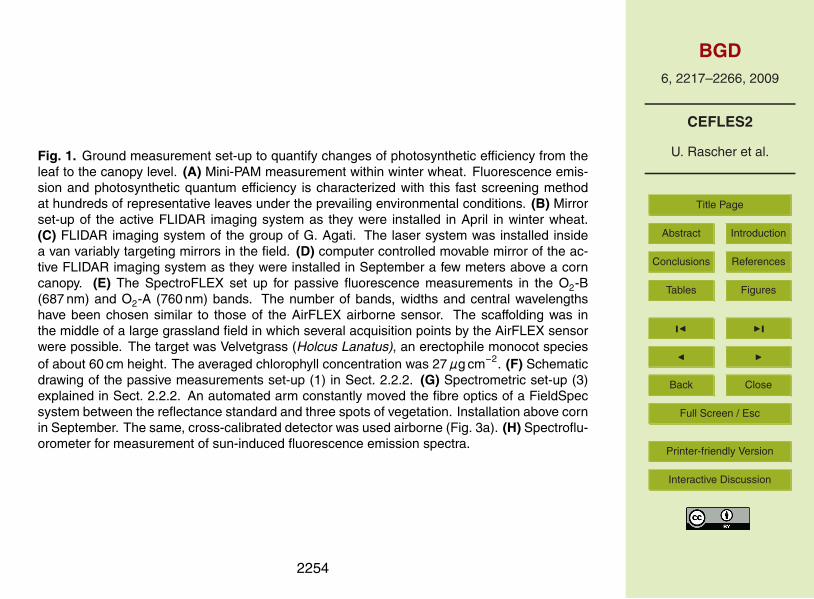
BGD6, 2217–2266, 2009

CEFLES2

U. Rascher et al.

Title Page



Tables Figures

J I

J I

Back Close

Full Screen / Esc



Fig. 1. Ground measurement set-up to quantify changes of photosynthetic efficiency from theleaf to the canopy level. (A) Mini-PAM measurement within winter wheat. Fluorescence emis-sion and photosynthetic quantum efficiency is characterized with this fast screening methodat hundreds of representative leaves under the prevailing environmental conditions. (B) Mirrorset-up of the active FLIDAR imaging system as they were installed in April in winter wheat.(C) FLIDAR imaging system of the group of G. Agati. The laser system was installed insidea van variably targeting mirrors in the field. (D) computer controlled movable mirror of the ac-tive FLIDAR imaging system as they were installed in September a few meters above a corncanopy. (E) The SpectroFLEX set up for passive fluorescence measurements in the O2-B(687 nm) and O2-A (760 nm) bands. The number of bands, widths and central wavelengthshave been chosen similar to those of the AirFLEX airborne sensor. The scaffolding was inthe middle of a large grassland field in which several acquisition points by the AirFLEX sensorwere possible. The target was Velvetgrass (Holcus Lanatus), an erectophile monocot speciesof about 60 cm height. The averaged chlorophyll concentration was 27µg cm−2. (F) Schematicdrawing of the passive measurements set-up (1) in Sect. 2.2.2. (G) Spectrometric set-up (3)explained in Sect. 2.2.2. An automated arm constantly moved the fibre optics of a FieldSpecsystem between the reflectance standard and three spots of vegetation. Installation above cornin September. The same, cross-calibrated detector was used airborne (Fig. 3a). (H) Spectroflu-orometer for measurement of sun-induced fluorescence emission spectra.

2254





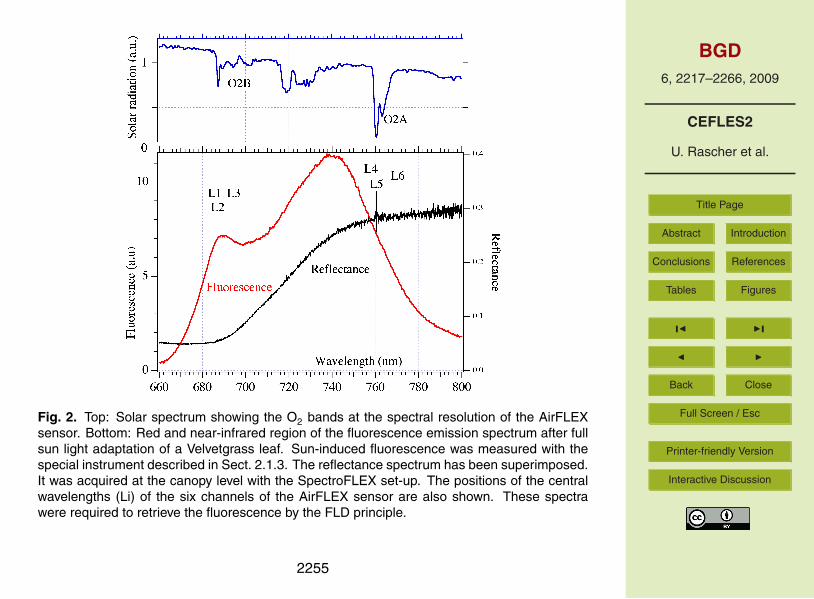
BGD6, 2217–2266, 2009

CEFLES2

U. Rascher et al.

Title Page



Tables Figures

J I

J I

Back Close

Full Screen / Esc



Fig. 2. Top: Solar spectrum showing the O2 bands at the spectral resolution of the AirFLEXsensor. Bottom: Red and near-infrared region of the fluorescence emission spectrum after fullsun light adaptation of a Velvetgrass leaf. Sun-induced fluorescence was measured with thespecial instrument described in Sect. 2.1.3. The reflectance spectrum has been superimposed.It was acquired at the canopy level with the SpectroFLEX set-up. The positions of the centralwavelengths (Li) of the six channels of the AirFLEX sensor are also shown. These spectrawere required to retrieve the fluorescence by the FLD principle.

2255





BGD6, 2217–2266, 2009

CEFLES2

U. Rascher et al.

Title Page



Tables Figures

J I

J I

Back Close

Full Screen / Esc



38

995 996

Figure 3. Airborne instruments that were employed during the campaign to quantify changes 997

of photosynthetic efficiency from the field to the regional level. A: Internal sensor head of the 998

AirFLEX sensor showing the six channels for O2-A and O2-B fluorescence retrieval. Each 999

channel requires three spectral bands: within the atmospheric absorption feature and on the 1000

Fig. 3.

2256





BGD6, 2217–2266, 2009

CEFLES2

U. Rascher et al.

Title Page



Tables Figures

J I

J I

Back Close

Full Screen / Esc



Fig. 3. Airborne instruments that were employed during the campaign to quantify changes ofphotosynthetic efficiency from the field to the regional level. (A) Internal sensor head of the Air-FLEX sensor showing the six channels for O2-A and O2-B fluorescence retrieval. Each channelrequires three spectral bands: within the atmospheric absorption feature and on the left andright shoulder of the absorption feature. (B) Picture of AirFLEX installed on board the CNRSENECA during the campaigns. (C) Thermal camera on board the SENECA. (D) INTA C-212-200 EC-DUQ “Paternina” aircraft. Within this aircraft both the AHS and HYPER sensor wereinstalled for parallel recording of flight lines. (E) AHS hyperspectral imager onboard EC-DUQ“CASA” as arranged during the CEFLES 2 campaign. (F) Picture of the SIM.GA HYPER sensor,which was first time used during the CEFLES2 campaign. (G) Underwing pod with the Field-Spec hyperspectral reflectance instrument. The instrument continuously acquired spectra with2 Hz resolution along repeated overpasses during the campaign. The same, cross-calibrateddetector was used on the ground (Fig. 1h).

2257





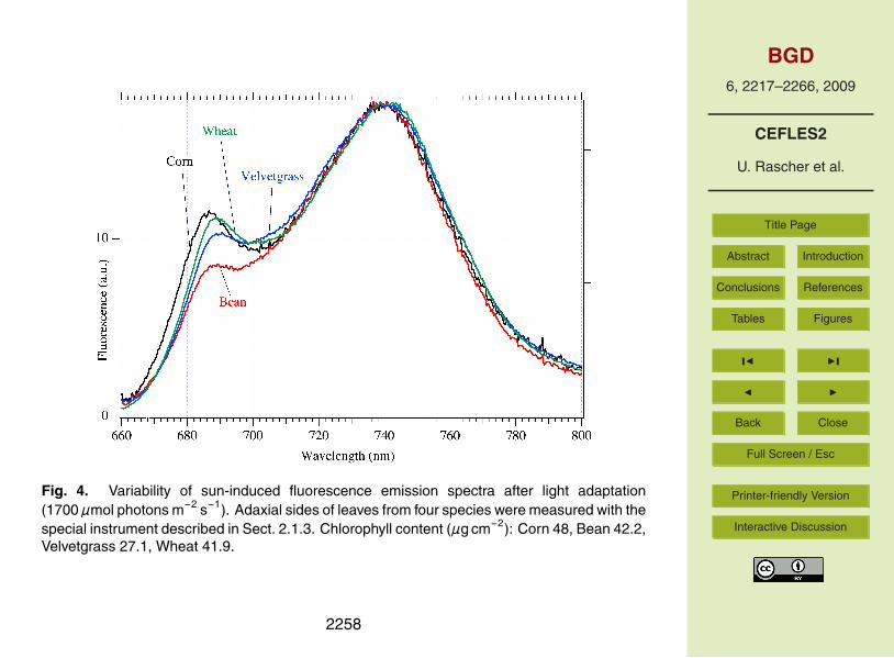
BGD6, 2217–2266, 2009

CEFLES2

U. Rascher et al.

Title Page



Tables Figures

J I

J I

Back Close

Full Screen / Esc



Fig. 4. Variability of sun-induced fluorescence emission spectra after light adaptation(1700µmol photons m−2 s−1). Adaxial sides of leaves from four species were measured with thespecial instrument described in Sect. 2.1.3. Chlorophyll content (µg cm−2): Corn 48, Bean 42.2,Velvetgrass 27.1, Wheat 41.9.

2258





BGD6, 2217–2266, 2009

CEFLES2

U. Rascher et al.

Title Page



Tables Figures

J I

J I

Back Close

Full Screen / Esc



41

1018 1019

Figure 5. (A): Diurnal course of fluorescence fluxes at 687 and 760 nm, (F687 and F760) and 1020

Photosynthetic Active Radiation (PAR), measured at the canopy level with the SpectroFLEX 1021

set-up. Similar results were obtained on 22 and 23 April, 2007. Vertical black lines indicates 1022

the moment at which the field has been flight over. The fluorescence ratios inboard and at 1023

ground level are compared in Table2. B, C: Diurnal courses of sun-induced fluorescence (Fs) 1024

and normalized Fs (Fs yield) at 760 nm measured over three measurement days. Values 1025

represent mean ± SE (n = 4 consecutive measurements). Measurements were collected over a 1026

Fig. 5. (A) Diurnal course of fluorescence fluxes at 687 and 760 nm, (F687 and F760) andPhotosynthetic Active Radiation (PAR), measured at the canopy level with the SpectroFLEXset-up. Similar results were obtained on 22 and 23 April 2007. Vertical black lines indicatesthe moment at which the field has been flight over. The fluorescence ratios inboard and atground level are compared in Table 1. (B), (C) Diurnal courses of sun-induced fluorescence(Fs) and normalized Fs (Fs yield) at 760 nm measured over three measurement days. Valuesrepresent mean±SE (n=4 consecutive measurements). Measurements were collected over awinter wheat dense canopy (LAI=6.3 m2 m−2) during three days of measurements (22–24 April2007) at the Marmande main site.

2259





BGD6, 2217–2266, 2009

CEFLES2

U. Rascher et al.

Title Page



Tables Figures

J I

J I

Back Close

Full Screen / Esc



Fig. 6. Sun-induced fluorescence and NDVI over different 11 agricultural crops and two ad-ditional surface classes. For each canopy type, average and standard deviation of 12 singlemeasurements were calculated (winter wheat 84, corn 96).

2260





BGD6, 2217–2266, 2009

CEFLES2

U. Rascher et al.

Title Page



Tables Figures

J I

J I

Back Close

Full Screen / Esc


Interactive DiscussionFig. 7. Laser induced fluorescence spectra of single corn leaves excited at 532 nm. (A) leavesat different position into the plant (I to VI from top of the plant). (B) Different part from the sameleaf (leaf II from the top).

2261





BGD6, 2217–2266, 2009

CEFLES2

U. Rascher et al.

Title Page



Tables Figures

J I

J I

Back Close

Full Screen / Esc



45

1042 1043

Figure 8. (A) Corn canopy area (about 1 m2) scanned by the FLIDAR imaging system, within 1044

small angles from nadir; note the presence of a fluorescence standard (blue) and a reflectance 1045

standard (white) at the left-top corner. (B-D) Canopy fluorescence maps at the 760 nm band, 1046

with excitation at 532 nm, acquired in sequence at 8:00, 10:30 and 15:00 (UTC), respectively, 1047

on 12 September, 2007. Each map, made up of 18 x 27 pixels, required an acquisition time of 1048

20 min. Fluorescence intensities in the colour bar are expressed as arbitrary units. 1049

1050

Fig. 8. (A) Corn canopy area (about 1 m2) scanned by the FLIDAR imaging system, withinsmall angles from nadir; note the presence of a fluorescence standard (blue) and a reflectancestandard (white) at the left-top corner. (B–D) Canopy fluorescence maps at the 760 nm band,with excitation at 532 nm, acquired in sequence at 08:00, 10:30 and 15:00 UTC, respectively,on 12 September 2007. Each map, made up of 18×27 pixels, required an acquisition time of20 min. Fluorescence intensities in the colour bar are expressed as arbitrary units.

2262





BGD6, 2217–2266, 2009

CEFLES2

U. Rascher et al.

Title Page



Tables Figures

J I

J I

Back Close

Full Screen / Esc



Fig. 9. Time evolution of photosynthetic CO2 uptake rate (A), leaf transpiration (B), SIF andLIF signals at 760 nm (C) and ratio of the fluorescence signals (D) from control and stressedcorn plants. Desiccation stress was applied at 10:00 UTC by cutting the plants but keepingthem under the same conditions in the canopy. Photosynthetic uptake rates and transpirationwere measured at the leaf level, while SIF and LIF were measured on the canopy level (about1×1 m). LIF and SIF data were normalized to a fluorescence standard signal and to the incidentsolar radiance, respectively.

2263





BGD6, 2217–2266, 2009

CEFLES2

U. Rascher et al.

Title Page



Tables Figures

J I

J I

Back Close

Full Screen / Esc



47

1061 1062

Figure 10. Top: AirFLEX transects over the Marmande test fields on 15 September, 2007. 1063

Bottom: Fluorescence flux at 687 nm, fluorescence flux at 760 nm and NDVI measured 1064

during the transect marked in red. 1065

1066

Fig. 10. Top: AirFLEX transects over the Marmande test fields on 15 September 2007. Bot-tom: Fluorescence flux at 687 nm, fluorescence flux at 760 nm and NDVI measured during thetransect marked in red.

2264





BGD6, 2217–2266, 2009

CEFLES2

U. Rascher et al.

Title Page



Tables Figures

J I

J I

Back Close

Full Screen / Esc



Fig. 11. Fs (left axis) and PPFD (right axis) averages at different hours of the day over 118pine fields (black circles) and over 47 wheat fields (white circles) during five days of flights from18–23 April 2007.

2265





BGD6, 2217–2266, 2009

CEFLES2

U. Rascher et al.

Title Page



Tables Figures

J I

J I

Back Close

Full Screen / Esc



49

1073 1074

Figure 12 Relative distribution of Fs signal as derived from HYPER imaging spectroscopy 1075

data (30 June 2007) without correction of anisotropic cross-track effects (top) and with 1076

empirical correction of the effects (bottom). Results show Fs values for all corn fields in the 1077

Marmande area and have been filtered with a 3x3 pixel mean filter to reduce statistical noise. 1078

Fig. 12. Relative distribution of Fs signal as derived from HYPER imaging spectroscopy data(30 June 2007) without correction of anisotropic cross-track effects (top) and with empiricalcorrection of the effects (bottom). Results show Fs values for all corn fields in the Marmandearea and have been filtered with a 3×3 pixel mean filter to reduce statistical noise.

2266





Documents

U. Rascher et al. CEFLES2: the remote sensing component …pubman.mpdl.mpg.de/pubman/item/escidoc:1692840/... · BGD 6, 2217–2266, 2009 CEFLES2 U. Rascher et al. Title Page Abstract