UNCL ASSI11!11FIED - apps.dtic.mil · 4.1 Review of Parameters and Effects 143 4.2 Design Procedure 145 4.2.1 Choosing T and U To Obtain a Given Directivity 145 4.2.2 Designing for

UNCL ASSI11!11FIED

41

U E

=OTICE: When governmnt or other drawi gs speci-fications or other data e used for any purposeother than in connection with a definitely relatedgovernment procurement operation, the U. z,Govenment thereby Incurs no responsibility., nor anyobligation mhatsoecver; and the fact that the Govern-ment May have formslated, furnished, or in any waymupplied the said drawings, specifications, or otherdata i not to be regarded by implication or other-wise as in mny mamer licensing the holder or anyother person or corporation, or conveying any rlgtsor Pe=nilson to manufacture, use or sell anypateted Invention that may in any way be relatedthereto.

ii

- ,K) ANTENNA LABORATORY

Technkal Report N4o. 52

ANALYSIS AND DESIGN OF THELOG-PERIODIC DIPOLE ANTENNA

EtinJ by

ROBERT V CARREL

Contract AF3(616).6079Proloct No. 9413.6279) Tak 40372

Sonsored by:AERONAL 't C SYSTEMS DIVISION

WRIGHT-PATTERSON AIR FORCEASE, OHIO

UNIVERSJTy 6F ILUNOIS

URILANA, ILLINOIS

OU

~1 AN~TENNA LABORATORY

U Technical Report No. 52

ANALYSIS AND DESIGN OF THE LOG-PERIODIC DIPOLE ANTENNAK1 byRobert L. Carrel

Contract AF33 (616) -6079

Project No. 9-(13-6278) Task 40572

ii Sponsored by:

[I AERONAUTICAL SYSTEMS DIVISION

ZlectricA1 E9ngineering Research LaboratoryZngiroering Experiment Station

Universityof IllinoistTjbata, Illinois

A--

ABSTRACT

A mathematical analysis of the logarithmically periodic dipole class

of frequency independent antennas, which takes into account the mutual

coupling between dipole elements, is described. The input impedance,

directivity, and bandwidth, as well as the input current and voltage of the

several elements, are calculated. A new concept, the bandwidth of the

active region, is formulaten and is used to relate the size and operating

bandwidth of the antenna. The limiting values oi the various parameters

that describe the antenna are ex plored. The results from the mathematical

model are shown to be in good agreement with measurements. A step by step

procedure is presented which enables one to design a log-periodic dipole

antenna over a u.de range of input impedance, bandwidth, directivity, and

antenna size.

ACKNOWLEDGEME.NT

The author wishes to thank all the members of the Antenna Laboratory

Staff for their help and encouragement. the guidance of his advisor, Professor

G. A. Deschamps, and the continued interest of Professor P. E. Mayes are

particularly appreciated. This work would not have been pvssible without

the timely invention of the log-periodic dipole antenna by D. E. Isbell,

whose counsel during tOe initial phase cf this research xas most helpful.

The author ts also fortunate to have been assotiated with V. H. Rumsey and

R. H. DuHamel during the time of their original contributions to the field

of frequency independent antennas.

Thanks are also due to Ronald Grant and David Levinson, student

technicians who built the models and performed many of the measurements.

This work was sponsored by the United States Air Force, Wright Air

Development Division under contract number AF33(616)-6079, for which the

author is grateful.

t4

iv

CONTENTS

Page

1. Introduction 1

2. Formulation of the Problem 15

2.1 Description of the Log-Periodic Dipole Antenna 152,2 Separation of the Problem into Two Parts 20

2,2.1 The Interior Problem 212.2.1.1 The Feeder Admittance Matrix 252,2 1 2 The Element Impedance Matrix 26

2.2.2 The Exterior Problem 332.3 Use of the Digital Computer in Solving 'he Mathematical

Model 37

3. Results and Analysis 39

3.1 The Transmission Region 39

3 1.1 Computed and Measured Results 403.1 2 An Approximate Formula for the Constants of an

Equivalent Line in the Transmission Region 52

3.2 The Active Region 553,2,1 Element Base Current in the Active Region 553.2.2 Width and Location of the Active Region 64

3.3 The Unexcited Region 713.4 The Input Impedance 77

3.4.1 General Characteristics of LPD Input Impedance 78

3.4.2 Input Impedance as a Function of T and Or 813.4.3 Input impedance as a Function of Zo and h/a 87

3.5 The Far Field Radiation 963.5.1 Radiation Patterns 98

3.5.1.1 The Characteristic Pattern as a Function

of T and Or 1153.5.1.2 The Characteristic Pattern as a Function

of Z and h/a 119

3.5.2 The Far Field Phase Characteristics 1273.5.2 1 The Phase Rotation Phenomenon 1?73.5.2,2 The Phase Cestvr 131

4. The Design of Lcg-Periodic Dipole Antennas 143

4.1 Review of Parameters and Effects 143

4.2 Design Procedure 1454.2.1 Choosing T and U To Obtain a Given Directivity 1454.2.2 Designing for a Given Input Impedance 1534.2.3 Application of the Design Procedure: An Example 154

4.3 Some Novel Variations in the Log-Periodic Design 181

5. Conclusion 168

vIV|

CONTENTS (Continued)

Page

Bibliography 171 1Appendix A 174 1

A.1 The Cosine-and Sine-Integral Functions 174A.2 Matrix Operations 179

Appendix B 181 iiB.1 Near Field Measurements 182

B.1.1 Amplitude Measurements 185B.1.2 Phase Measurements 187

B.2 Impedance Measurements 193

B.3 Far Field Measurements 195

vi

ILLUSTRATIONTS

Figure Page

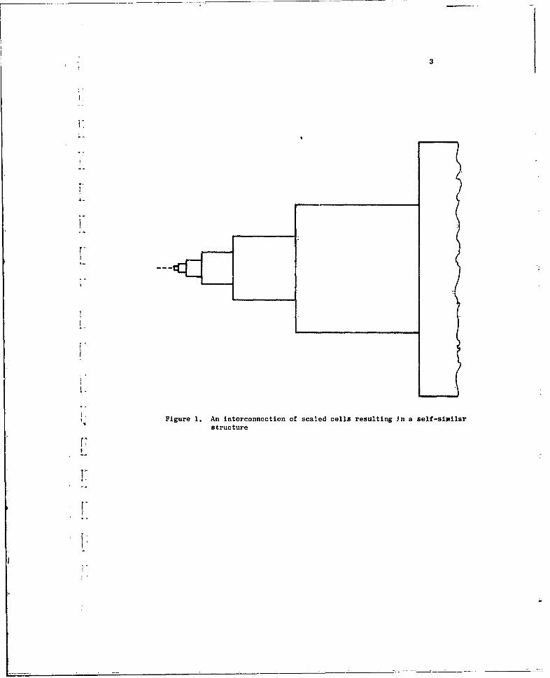
1. An interconnectLon of scaled cells resulting in a self--similar structure 3

2. Infinite bi-cone and bi-fin structures 6

3. A balanced planar log-spiral antenna. The shaded portionrepresents one cell 8

4. A planar log-periodic antenna 10

5. A non-planar log-periodic antenna 11

6. A log-periodic dipole antenna 12

7. A picture of a log-periodic dipole antenna 16

8. A schematic of the log-periodic dipole antenna, includingsymbols used in its description 'L7

9. Connection of elements to the balanced feeder and feedpoint details 19

10. Schematic circuits for the LPD interior-problem 22

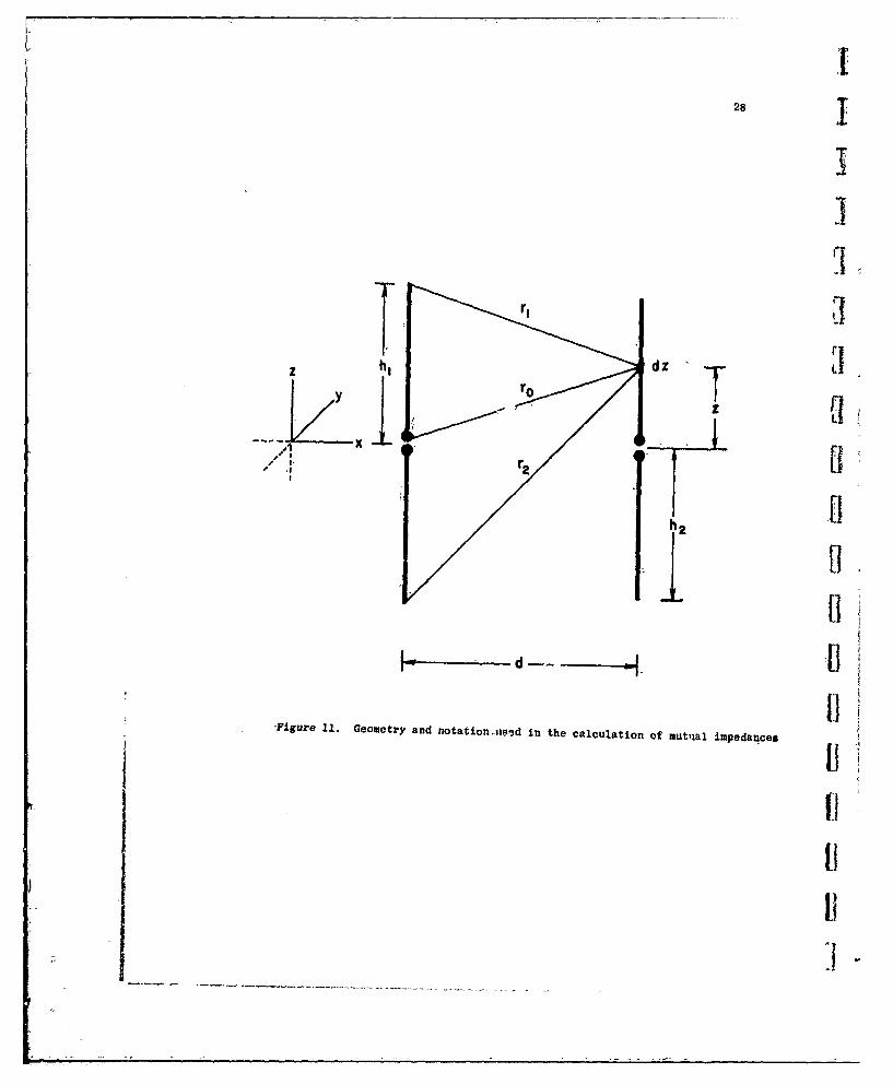
11. Geometry and notation used in the calculation of mutualimpedances 28

j 12. Geometry and notation used in the calculation of selfimpedances 32

13. Coordinate system used in the computation of the far fieldL radiation patterns 35

14. Sketches of the transmission- and radiation field lines 41

15, Computed and measured amplitude and phase of the transmissionwave vs. relativ? distance from the apex at frequency f3 ;T = 0.9.&, = 0,0.64 Zo = 100, Z = short at h /2 h/a = 177 42

16. Computed and measured amplitude ai,'d phase of the transmissionrave vs. relative distance from the apex at frequency ff3 1/41

0.95, O = 0.0564 N = 13, Zo = 100, ZT = short at hj/2,h/a = 177 44-

17. Computed and measured amplitude and phase of the transmissionwave vs. relative distance from the apex at frequency- f3 1/2T = 0.95, O = 0.0564 N = 13, Zo 100, ZT = short at h1/2)h/a = 177 45

11M

vii

ILLUSTRATIONS (Continued)

Figure Page

18. Computed 2nd measured amplitude and phase of the transmissionwav vs. relative distance frsm the apex at frequency f3 3/4;T = 0.95, = 0.0564 N = 13, Zo = 100 Z = short at hl/2h/a = 177 T 46

19. Computed and measured amplituue und phase of the transmissionwave vs. relative distance from the apex at frequency f4 ;

= 0.95, a = 0.0564, N = 13 Zo = 100 Z T f= short at hl/2,h/a = 177 47

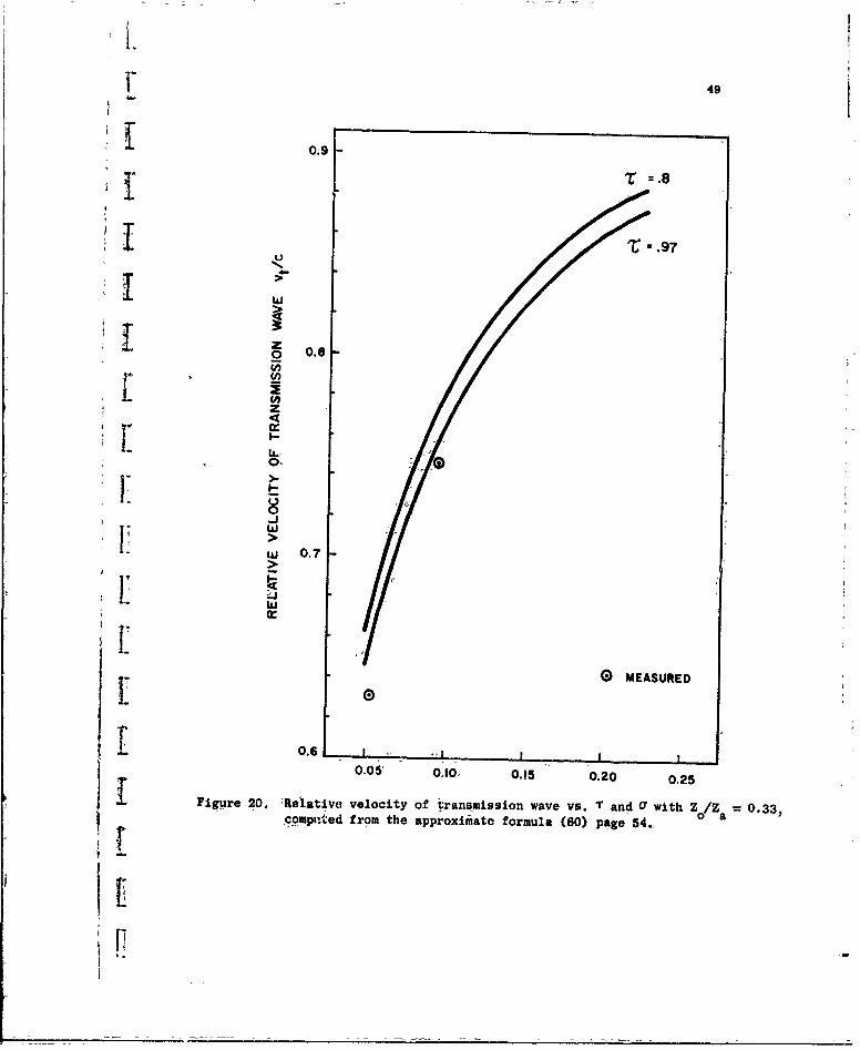
20. Relative velocity of transmission wave vs. T and a computedfrom the approximate formula 49

21. Computed and measured amplitude and phase of tLe transmissionwave vs. relative distance from the apex at frequency f3;T = 0.888, = 0.089, N = 8j, Z o = 100, ZT = short at h/2,

h/a = 125 50

22. Relative velocity of transmission wave as a function of therelative phase velocity along the feeder with the elementsremoved. 51

23. Computed base impedance Zb vs. eloment number for an eight )element LPD at frequency f4 56

24. Computed and measured amplitude and phase of the element

.!se current vs. relative distance from the aoex, at ire-qun.cy f.; T = 0.95, O = 0.0564, Z = 100, h/a = 177, ZT =short -cuit at hl/2 0 58

25. Computed and neasured amplitude and phase of the elementbase current vg.- elative distance from the apex, at frequencyf 1 = 0.95, a = 0.0564, Zo = 100, h/a = 177 ZT = shortchriWt at h, 59

26. Computed and measured amplitude and phase of the element basecurrent vs. relative distance from the apex, at frequencyf3 1/2 1 9 I0o95, a z 0.0564,Z o = 100 h/a = 177, ZT = shortcircuit at h /2 60

27. Computed and measured amplitude and phase of the element basecurrent vs. relative distance from the apex at frequencyf ; 'i - 0.95, a = 0.0564, zo = 100 h/a = 177,z = short

circdt at hi!2 61

28. Computed and measured amplitude and phase of the element basecurrent vs. relative distance from the aper:at frequency f4

= 0.95, 'Tf-00564 Zo = 100, h/a -177, ZT = short circuit

at hl/2 62

viii


Figure Page

29. Relative amplitude of base current in the active region vs.element number, frequencies fl thru f6. T = 0.888, a = 0.089,

N = 8, Zo = 100, k/a = 125, ZT = short at hl/2 63

L 30. Computed relative phase velocity of the first backward spaceharmonic in the active region vs. a for several values of T. 65

31. A typical curve of base current vs. distance from the apex,showing the quantities used in the d;ifinition of the bandwidthand location of the active region 68

32. Bandwidth of the active region, Ear, vs. U and r 70

33. Shortening factor S, vs. Z and h/a 72

34. Radiating efficiency of the active region vs. relative lengthof the longest element 75

35. Radiating efficiency of the active region vs, feeder impedanceand T 76

1. 36. Input impedance vs. frequency of an eight element LPD 79

37. Input impedance showing periodic variation with frequency 82

38. Input impedance R vs. O and T for Z = 100 and h/a = 177 830 0

39. Difference between the approximate discrute formula andapproximate distributed formula for R , vs. the distance

botween elements as a percent of the ?atter 85

40. Computed SWR vs. a and T for Z = 100 and h/a = 177- 86

41. Input impedance Ro vs. feeder impedance Zo, T 0.888, o =

. 0.089, N = 8 h/a = 125 88

42. Input impedance R vs. Z0 and a, with h/a = 177, from theapproximate formua 89

43. Input impedance R0 vs. h/a and a, Zo = 100, from the approxi-mate formula 9

44a. Inp3ut lmpedance T = 0.888, a = 0.089, N = 8, Zo = 50, ZT =50at frequencies f3 1 f4, f4 1/2 , f5 and f6 92

44b. Input impedance T = 0.888, a = 0.089, N = 8 , Zo = 50 ZT=short at hl/2, at frequencies f3, f4, f5 and f6 33

- 45. Average characteristic impedance of a dipole Z vb. heightto radius ratio h/a a 94

ILLUSTRATIONS (Continued) ix

Figure Page

46. Relative feeder impedance Z0 /R0 vs. relative dipole impedanceZaJRo, from the approximate formula, 95

47. A frequency independent 4:1 balun transformer for use with

LPD antennas 97

48. An example of radiation patterns computed by ILLIAC, 7 =

0.888, a= 0.089, i = 8, Z° =l100 ZT = short at h1 /2 99

49. Computed patterns T = 0.888, a = 0.089 Z0 = 100, Z = shortat hl/2, showing no difference between patterns for = 5 andN =8 100

50. Computed half power beamwidth vs. frequency; T - 0.888, a' =0.0891 N = 8, Z° = 104 ZT = short at h1/2 101

51. Computed and measured patterns; T = 0.888, Or = 0.089, Z =

100, ZT short at h /2 0 103

52. Computed and measured patterns; 'r = 0 888, a' = 0.089, Z =100, ZT = short at- 11h/2 0 104

53. Computed and measured patterns; T 0.888, a = C.) 089, Z100, Z = short at bl/2 105

T

54. Computed and measured patterns; T = 0.888, o = 0.089, Z 106

100 ZT = short at h1 /2 106

55. Computed and measured patterns; T = 0.888, a' = 0.089, 0 =I00. ZT = short at hi/2 107

56. Computed and measured patterns; T = 0.888, a = 0,089P Z =100, ZT = short at h,/2 108

57. Computed and measured patterns; T = 0,98, a = 0,057, N = 12,Z =100 ZT = short at h1/2 109

58. Computed and measured patterns; + 0.98, a' = 0.'057, N = 12,Z° =100j ZT = sho t ah/2 110 d

59. Computed and measured patterns; T = 0.98p 0' = 0.057, N = 12,

Zo = 1001 ZT 1 short at h1/2

60. Computed and measured patterns; T = 0.8, a' = 0.137, N = 81Z = 100 Z =short at h /2 1120 T 1

61. Computed and measured patterns; T 0,8, 0' = 0.137, N = 8,Z = 100, ZT = short at hl/2 1130 1

6.Computed and measured patterns; T = Q8p a = 0.137, N = 8,) 1Z0 10, Z T short ath,/211

x


Figure Page

63. Computed E-plane half-power beamwidth Vs. T and U; Z = 100)ZT = short wt h1r 2 , h/a = 177 116

64. Computed H-plane half-power beamwidth vs. T and 0; Z° 100)ZT = short at h/2 h/a = 177 117

65. Computed contours of constant directivity vs. T, a, and Q;Z = 100, ZT = short at h /2, h/a = 177 118

0TI

:66. Measured patterns; T = 0.7, U = 0.206, Z = 100, ZT shortat h,/2, N =-6, h/a 177 120

67. Computed and measured H-plane patterns: 7 = 0.7, 0 = 0.206Z 100, ZT = 100 N = 6, h/a = 177 121

68. Computed pattern front to back ratio vs. 0 and T; Z = 100,ZT = short at hl /2 122

69. Computed and measured patterns; T = 0.888) a = 0.089 Z=150, ZT = short at h1/2 0 123

'7n. Computed and measured patterns; r = 0.888p = 0.089 Z0150, ZT = short at h /2 124

71. An example of computed-and measured directivity vs. h/a 126

72, Computed far field phase as a function of frequency, illu-strating the phase rotation phenomenon 130

73. Coordinate system for phase center computations 132

74- A typical evolute of an equiphase contour, plotted on a

wavelength scale 135

75. Typical frequency variatior of the relative distance fromthe apex to the phase center 136

76. Measured and computed location of tlht phi6 uetta WitLh-reference to the active region 138

V 77. Location of the phase center in wavelengths from-the apex 139

78. Coordinate system for the computation of the phase tolerLnce 140

79. Nomograph, a = 1/4(1 - T)cot a 148

80. Nomograph, B = 1.] + 7.7 (1 - T)2 cot Q 149

) ar

81. Nomograph, L/X = 1/4(1 - -) cot C 150max B


Figure Page1

82. Nomograph, N = 1 -t (log B s/lOg) 151515T

83, The LPD realized by the design procedure of Section 4.2.3 157

84. Measured standing wave ratio vs. frequency of the designmodel 158 j

85. Measured- E- and H-plane half-power beamwidth and directivityof the design model 159

86. Computed and measured patterns of the design model 160

87-. Two LPD antennas in cascade 162

88. An LWD antennaetched from double- copper-clad Rexolite 164

89. Measured- patterns of an LPD antenna which was etched from

double copper-clad Rexolite 165

90. Measured patterns of an LPD- antenna which was etched fromdouble copper-clad Rexollte 166

91. Computation time-vs. argument x--for the series and continuedfraction expansion of K(x) = Ci.(x) + J Si(x) 175 -

92. A picture of one of the antennas used for near -fieldmeasurements 183 i

93. Details of the probe used for-measuring the voltage between

the feeder conductors 184

94. Details of the probe used for measuring the dipole element '1

current 186

95. A block diagram of the amplitude measuring circuit 188

96. A block diagram of the-phase measur -g circuit 189 -

97. Phasor relations and- the nulls obtained for values ofIETI/IER! for two methods of-measuring relative phase. ETis- the test signal, ER is the reference signal 190

98. -A picture of the equipment arrangement used in the near fieldmeasurements 192

99. Details of-the symmetrical feed point, showing the reference

plane -foi, impedance measurements 194

100. Antenna positioner and-tower at the University of Illinois!

Antenna Laboratory 196 5

I i--. .. ...- £

1. INTRODUCTION

The-object of this work is to provide a mathematical model of the

log-periodic dipole antenna which contains the essential features of the

practical antenna and which is amenable to solution. The need for such

a-viodel occurs for two reasons. First, the principles of lig-periodic

antenna design have evolved from the interpretation of laboratory measure-

1 ments, without the benefit of mathematical analysis. A rigorous formulation

of these principles is clearly called for. Second, the task o' extending

the state of the design art if log-periodic antennas, is formidable if

I carried out on a wholly experimental basis. Even an approximate analysis

is quite useful if it lends direction to an explrimental program. The

conclusions resulting from the solutioihof the mathematical model proposed

herein are sufficiently general to lend insight into the operation of

log-periodic dipole antennas, and- the results are applicable to the

V design of LP dipole antennas which must meet given electrical specifications,

Throughout this work it becomes necessary to define as precisely as

possible certain concepts relating to wideband ant pnas, such as "broadband",

"frequency independent", "active region", and "end effect". Some of the

terms have been objects of disagreement over the past years, and while

-the definitions heretnmay not settle the issue, they can provide a

common ground of understanding for this work. The terms "wideband" and

"brnAdband" have become so much- a mart --f c a -_.-.. g vernacular

that they express only a notion and must be qualified each time they are

-used. In the follcwing paragraphs the term "frequency independent" is used.

Strictly speaking, there are no frequency independent antennas. However, it

21

is proposed that a xore liberal definition be adopted-one which applies T

to a special class of antennas. By frequency independence as applied to

an antenna, it is meant that the observable characteristics of the antenna

such as the field pattern and input impedance vary negligibly over a band

of frequencies within the design limits of the antenna, and that this

bLnd may be made arbitrarily wide merely by properly extending the geometry T

of the antenna structure. The ultimate band limits of a given design are

determined by non-electrical restrictions: size governs the low frequency

limit., and precision of construction governs the high frequency limit.

The idea of frequency independent antennas is based upon the familiar

Ioperation of scaling and the principle of similitude . -It is well known

that the performance of a lossless antenna remains unchanged if its dimensions

in terms =f wavelength are held constant. Thus, If all dimensions of a

lossless antenna are decreased by a factor T < 1 , and the frequency is

increased by l/T, the fields about the two antennas are similar, that is,

they differ at most by a constant factor Consider a class of structures

which are made up-of an infinite number of interconnected "cells" such as

shown in Figure 1. Each cell is similar to its neighbor by a constant Iscale factor T, Structures of this class are called self-similar because

they possess the unique property of transforming into themselves under a

uniform expansion by T or an Integral power of T. If each cell represents

an electromagnetic apparatusY the performane of the structure remains the

same for all frequoncies related by

fO p , t 1, + 2,. 1f -o

If the structure is a source or sink of electromagnetic waves, then each

:I'

3

7

* Figure 1. An interconnection of scaled cells resulting Jn a self-similarstructure

f;

F-

I-

4

cell may centain lumped or distributed generators or loads. To preserve

similitude, a generator at frequency f in cell n must "scale" into a0

generator at frequency Tf0 in cell n + 1. If it is undesirable to move

the generators about, an excitation independent of scaling can be obtained

by placing a generator at the small end of the strunture. Only the latter

method of excitation will be considered.

luch self-similar structures exhibit what is calld, log-periodic

performance. Although the patterns and input impedance may vary with

frequency, the variation must be periodic with the logarithm of frequency.

In order for the pattern and input impedance to be independent of frequency,

the variationjh.performance over the period, log T, must be negligible.

To be a practical antenna, the infinite structure must be truncated.

That is, the scaling must start with a given small cell ard must stop at

a given large cell. The requirement that the truncated structure must

duplicate the performance of the infinite structure places certain restric-

tions cn the nature of the cells in the aggregate. At a given frequency the

electrically small eells must behave as a transmis ...n line. Truncation at

the small end is equivalent to the elimination of a section of line; the

net effect is a shift in the location of the generator. The electrically

large cells mtist be unexcited, so that their presence or absence makes

no difference in'the electromagnetic performance at the given frequency.

When this is true, thp fact that the structure has an end will not be

observable, and the "end effect" is said to be eliminated. The foregoing

restrictions on the small and large cells require that:most of the energy

be radiated from a limited number of adjacent, "medium-sized" cells. These

p%

5

cells constitute the "active region". Thus three riegions may be associated

with the infinite, self-similar structure-the "transmission region", the

"active region", and te "unexcited region". The key problem, therefore,

is to determine which finite stru'tures, if any, exhibit performance which

approaches that of the infinite structure over a design band.

-Let the steps be traced which led to the discovery of several types

-- of frequency independent antennas, leading up to the log-periodic dipole

antenna. Prior to 1954 much effort had been expended in attempts at

antenna broadbanding. These efforts, for the most part, applied the

comparatively advanced knowledge of broadband circuit theory to basically

narrow band antennas. Some notable examples resulted2'3 . However,

conventional antennas resisted efforts to extend the usable bandwidth

V ratio beyond two or three to one.

In the fall of 1954 Rumsey broke the bandwidth barrier in antenna

theory and practice with his "angle method"4 . He stated that if the shape

of an antenna were such that it could be specified entirely in terms of

angles it would exhibit constant input impedance and pattArns independent

fj of frequency because no fixed length is involved in its description. The

infinite bi-conical and bi-fin structures shown in Figure 2 are frequency

bindependent, ut infinite structures are not practical antennas. If

one truncates these structures, the frequency independent behavior is

lost; the patterns vary with frequency. The variation with frequency is

a manifestation of the "end effect", that is, the effect of radiated

and/or reflected current at the discontinuity introduced by the truncation.

Rumsey suggested- that the log-spiral curve defined by r = exp(kO could

6

9 9

ILzi

zz

Fiur 2.7fnt:1cn nd~ifnsrcue

7

be used to define another infinite structure in terms o£ angles only. He

also showed that the log-spiral family of surfaces are the only surfaces

for which an expansion is equivalent to a rotation. For a rotation about

the = 0 axis this can be expressed symbolically as

r = f(6,0 =,.e-acf(erp+ c) (2)T_

U The pattern of such a structure rotates with frequency about the e 0

axis at a rate which depends on a. A balanced, planar log-sptral antenna

is shown in Figure 3.

r The log-spiral is an example of a self-similar siructure. One cell.

of the structure is given by the shaded portion of Figure 3. The fact

that the exiansion from one cell to another can also be accomplished by

a rotation sets the log-spiral apart from other self-similar structures

in which the expansion must be carried out in a fixedodirection. In

contrast to the bi-cones and bi-fins, the truncated log-spiral structure

is one antenna whose pattern is the same as that of the infinite structure

for all wavelengths shorter than twice the length of the truncated spiral

jr arm. The. absence of end effect is the result of a rapid diminution of

current along the spiral arm. The radiation pattern of the planar log-

spiral is bi-directional and centered about theO8 = 0 axis. Over a wide

range of design parameters the pattern is rotationally symmetric and

circular-lv volarized. The sense of the circular polarization is in tho

negative ( direction for the log-spiral of Figure 3. The properties of

planar and conical log-spiral antennas have been carefully investigated

and 78and catalogued by Dyson

Ir 1956 DuHamel considered the possibility of perturbing the smooth

geometry of the bi-fin antenna In order to produce a rapid diminution of

(-

#,=90* .

I I

if

Figure 3. A balanced planar log-spiral antennaThe shaded portion represents one cell t

,!f

j

9

current on the structure. He first considered planar structures which,

if extended to infinity, were self-complementary. This was in order to

assure a frequency independent input impedance. Figure 4 shows one such

structure which consists of a plurality of teeth and slots cut in a bi-fin

in such a manner that the widths of successive teeth and slots form a

geometric progression. This self-similar structure was called a log-

periodic antenna because its geometry repeats periodically with the

logarithm of the distance from the apex. The trui-ated structure exhibited

patterns and impedance which varied periodically with the logarithm of

frequency; and for a wide range of parameters the variation over a period

was negligible, yielding frequency independent operation. The teeth and

slots accomplished the necessary reduction of end effect. The radiation

pattern of the planar -LP is characterized by a bi-directiusial beam centered-

on the 0 = 0 axis. The antenna is horizontally polarized when oriented

as shown in Figure 4, Thus the polarization of the planar LP is

orthogonal to the polarization of the smooth bi-fin.

An attempt at providing a uni-directional pattern led -to the nonm

101, planar LP..tructures which Isbell investigated. The antenna shown in

Figure 5 exhibits a horizontally polarized uni-directional beam off the

tip end. Again, a lack of end effect is observed and the patterns are

frequency Independent over a range of the design parameters. In the

LPD antenna of Isbell". shown in Figure e. dipole elements replace th~e

teeth of the non-planar LP and a constant impedance two-wire feeder

replaces the central bi-fin section. One observes the frequency independent

behavior of the LPD antenna over large ranges of the design parameters.

10 I

II

I

.19 .0 1

06i

-~ 900

0-900

Figure 5. A non-planar log-periodic antenna

I12 1

-i

-i

Iif

4)4., 1-4a-4

-4U.4) 1.4)0-4

4)

0'-4

.4:.

iii[1[IIII11F 'II

IIII

13

Table 1 summarizes the preceding discussion by a classification of self-

similar structures. There are some finite structures that exhibit only

log-periodic electrical characteristics and others that have log-periodic

geometry but neither frequency independent nor log-perlodic performance,

:* Experience has shown that the latter category contains many members.

- The log-periodic dipole antennu was selected for analysis because it

is made of conventional linear dipole elements, a fact which allows one

to replace the tubular conductors with filamentary currents. In this work

electromagnetic field theory is used to calculate the self and mutual

I.. impedances of the several dipole elements from an assumption of a sinusoidal

- form of current on each element. Circuit -techniques are used-to find the

voltage and current at the terminals of each dipole element and the

I antenna input impedance. Once the element current is known, field

techniques are again used to calculate the radiation pattern.

The organization of this work is as follows: The preceding section was

an introduction to the idea of frequency independent antennas. In Section

2 the mathematical model of the LPD antenna is formulated using the self

and mutual impedances of the several dipole elements. The expressions

for input impedance, and voltage and current at th-e base of each element

are determined. The equaions for the radiated field and the phase center

are also set up. In Section 3 the computed anC measured results are

displayed and analyzed. Criteria for "optimum" LPD antennas are established.

Section 4 presents design information, combining the computed and measured

results in simplo formulas and nomographs. Section 5 summarizes the work.

Appended is a section which considers the computation-of the equations of

Part 2, and a section devoted to the measurement techniques used in this

research.

C: 0 0 0 0 0 .14.4 41 -H 4. 41 44J

C) a .4 4 .4 0cd

U :4 .4 .4 V V.4

-0 14 0

0'

9-4 9-4 '-4 U30020 44C 0 0c

)C,0 v 9: "4:4 -------'to c

c u

4. 0

V4 ~ 44 0 0

U.. Uk40 0.4 0 4 .2~~~ 4J.) 0 . 4

C) U 4 4.44

V.4 0 0

U~~. 0* 0 I,*' '' ~ -U. c, !00 bbI) I" ;n R 4-4 k- CC 0

U ~ ~~ ~~~~ 0 .S. S. 4. 4* S.U iU'~9 C)f 4

2 0.

0104

15

2. FORMULATION OF THE PROBLEM

2.1 ICscription of the Log-Periodic -Dipole Antenna

The log-periodic dipole antenna, shown pictorially in Figure 7 and

described by Figure 8, consists of a plurality of parallel, linear dipoles

arranged side by side in a plane. The lengths of successive dipole elements

form a geometric progression with the common ratio T < I. T is called the

scawle factor. A line through the ends of the dipole elements on one side of

-the antenna subtends an angle a with the center lire of the antenna at the

virtual apex-0. The spacing factor T is defined as the ratio of the distance

between two adjacent elements to twice the length of the larger element, and

is a constant for a given antenna, The geometry of the antenna relates O to

T and a.

a (I - T)cot a (3)

4

The largest element is called element number i. The half length of

element n is denoted by h Therefore,

h =h Tnl (4)

The distance d from element n to element n + 1 is given byn

dn = dIl- (5)

Ifa nis the radius of element number n, the a n s are given by

a= a-n 1 U

The ratio of element height to radius is the same for all elements in a

given antenna and will be denoted by h/a,

The elements are energized from a balanced, constant impedance feeder,

161

Aill

SYS

14

:)4

34

6 V1

17

DIRECTION OF BEAM

41 I _ I i ,( % .Yii lii

ndn

Xn n r h n xt/2

Xn -i !dn

METHOD OF FEEDING,

Figure 8. A schematic of the log-periodic dipole antenna, 'includingsymbols used in its description

adjacent elements being connected to the feeder in an alternating fashion.

Due to the alternating mariner in whicn the elements are connected to the

feeder, one cell of tne LPD antenna consists of two adjacent dipoles and 'Itwo sections of feeder. Thus T as defined above is the square root of the

cell scaling factoro Ideally, the feeder should be conical or stepped, .1to preserve the exact scaling f-om-onA l1 t the-nexNt. -Rowever, it has

been found in practice that two parallel cylinders can satisfactorily

replace the cones as long as the cstlnder radius remains small compared

to the shortest wavelength of operation. The element feeder configuration

is shown in Figure 9. It is seen that the elements do not lie precisely ii-ina plane; the departure therefrom is equal to the feeder spacing, which Iis always small.

The antenna may be energized from a balanced twin line connected at

the junction of the feeder and the smallest element. Alternatively, a

coaxial line may be inserted through the back of one of the hollow feeder

conductors. The shield of the coax is connected to its half- of the feeder

at the front of the antenna, the central conductor of the coax is coanected

to the other side of the feeder as shown in Figure 9 -In the latter method

the antenna becomes its own balun because the currents on the feeder at the

large'end of the antenna are negligible, as will be demonstrated later.

Due to the diminution of current at the large end, the impedance Z T which Iterminates the feeder at that point is immaterial. For definiteness,

in most models ZT will be taken equal to the characteristic Impedance Z 0

of the feeder. The'propagation constant of the feeder alone is-B and

may be different from the free space propagation constant B-if dielectric

is used.

II 19

FEED

Figure 9. Connection of elements to the balanced feeder and

feed point details

20

When the antenna is operated at a wavelength within the design limits,

that is approximately

4 hN < < 4h (7)

where N is the total number of elements, a linearly polarized undirectional 4beam is observed in the direction of the smaller elements. It is found that

for any frequency within the design band there are several -elements of

nearly half-wavelength dimensions. The current in these elements is

large compared to the current on the remainder of tie elements; these Ielements contribute most of the radiation, and form the so-called "active

region". As the frequency is decreased from fn to Tf the active region

shifts from one group of elements to the next. In most cases the variation

in performance over a log-period is negligible and frequency independent

operation results. Since the LPD antenna is a truncated section of the .1infinite structure, the performance of the antenna approaches that of the

infinite structure only to the extent that a properly constituted Active

regioi exists on the antenna. The active region becomes deformed as it

begins to include,the- smallest or largest element on the antenna. When

-this happens, the upper or lower frequency limit is reached. and it is this

phenomenon which detarmines the useful bandwidth of the antenna. I2.2 Separation of the Problem into Two Parts

The problem may be divided into two parts for the purpose of simplifying jthe analysis. Finding the voltnoes and currents -along -the -foder constitutt:3

the interior part of the problem, and finding the field of the dipole

elements constitutes the exterior part of the problem.

21

Since the feeder has transverse dimensions which are small compared

to wavelength, its principal function is to guide and distribute the energy

to the radiating elements. There is negligible inductive and capacitive

coupling from the feeder to the shunting rlonwents because the fields due

to the currents and charges on the feeder are very small at the location

of each dipole element.

In the exterior problem, the magnitude and phase of the far field

radiation produced by the currents on the elivvints are of primary interest.

The E- and H-plane beamwidths, directivity, front to back ratio, and side

lobe level can be determined from the radiation pattern. The phase center

L can be determined from the phase of the far field.

2.2.1 The Interior Problem

Insofar as the interior problem is concerned, the connection of the

dipole elements to the feeder Is equivalent to the parallel connection of

two N terminal-pair circuits. One circuit consists of the feeder with

alternating, properly spaced taps which represent the terminals to which

he elements are eventually attached. The feeder circuit is shown schematically

in Figure lOb, and includes the arbitrary terminating impedance Z . The

other circuit) shown schematically in Figure lOa, Tepresents the behavior

of the dipoleelements as viewed from their input terminals.

Let Y be the admittance matrix of the feeder circuit. Then

F

LF = -V (8)

where I and V Fare column matrices which represer'. the 11 driving currents and

I22

ANTENNA / EL ENTS

'A! ~ 'A 'A2' t ' 113 11 'A NO4.- 4<-" 4 4

'AI "'vA2 "'A3 "AN

a. ELEMENT CIRCUIT "'V L "VL2 OV L3 "VLNI " LI 1L2 L3 'LN4

cciTA

.d - t.-F, *- -- -----

b. FEEDER CIRCUIT

NI10

c. COMPLETE CIRCUIT

Figure 1 . Schematic circuits for the LPD interior problem

23

response voltages of the feeder circuit. Let YA be the admittance matrix

of the element circuit. Then

I A AA(9)

where I and are coluvmi itwtrices which represent the driving currents

T and resp6ose voltages of the eleman circuit. If the corresponding terminals

of the feeder and element circuits are €oncted in parallel, a new circuit

is obtained as shown in Figure lOc. The new resnonse voltage matrix is

equal to either A or V F since they are equivalent. The new driving

current matrix is now the sum of I and TF due to cosi.ervation of current

at a node. If Equations (8) and (9) are added,

I = A + I F = YYAVA + YFVF . (10)

F is set equal to and factored,

I=(A+ Y )VA(1

TA) the base current at the dipole element terminals, is of primary interest.

Therefore

f (A + F )AA (12)

where Z - Y Multiplying Z- iside the paeenthesis results inA A A

Y (V + YFZA) A (13)

where U is the unit matrix.

24 ,1

The elements of I represent the input currents at the terminals of the

new circuit of Figure 10c In the actual LP antenna all I ns are zeroniexcept iNJ the current at the feed point, which is the driving current of

-the antenna. The driving current may be set equal to one ampere. Therefore,

00o 10

1= "(14)

• IL

1

Equation a3) must be solved for TA. This can be done by inverting the Amatrix T,

F U FA' (15)

and multiplying

1 -1

TA =fT I (16)

or by solving directly the set of simultaneous Equations (13). The latter I

method is preferable in terms of computarx6n time and accuracy due to the

special form of 1.

Once I is determined V can be found by multiplyingA A

V -ZI(17)VA = AIA

Note that 7F (ffVA) is not the voltage between the two feeder members at

I

25Veach element, but differs therefrom by a phase change of 180 at every

other element. The Nth element of V A is the voltage across the smallest

dipole; it is also the input impedance of the entire antenna since one-

ampere of driving current was assumed.

The Interior problem has beei £ozmulaLted and its solution -indicated.

It remains to determine explicity the feeder admittance matrix and the

element imr,%dance matrix.

2.2.1.1 The Feeder Adimittance Matrix

The admittance matrix for one section of transmission line of length d,

propagation constant 80, and characteristic admittance Y is

00

J Y cot B d + Y csc 8 d0 0 0 0

= (18)

+ J Y csc B d - J Y cot 8ed

Connecting N-i of these sections according to the scheme shown in Figure 10

results in the following matrix.

(YT-JY cot Bod') -JY csc Bed 0 0

-JY csc Bod -JYo(cot-od1 JYo csc 0od ... 00 0o1 00 0 o2

+ cot Bod2)

0 -JYo csc Bed -J0(cot Bed 2 ... 0

+ cot Bed 3)

oN-

0 0 0 ""-JYo cot 3d

(19)

I

26

YTP the terminating admittance, has been added in y11 " All tb, eldednnts off

the diagonal by two or more are zero because yi is the current in terminal

i due to a unit voltage at j, all terminal pairs other than j being shorted.

The short circuit restricts current flow to sections of line adjacent to

the terminals to which the voltage is applied; hence no voltage is induced

in the remaining sections. -

2.2.1.2 The Element Impedance Matrix

The seif anu mutual impedances oA tn dipole elements are calculated-

12using the method of &nduced-emf . The following approximations are made

in this method: j

1. A symmetric sinusoidal current distribution is assumed over the 1length of each dipole. This assumption is valid as long as the dipole is

reasonably less than a full wavelength long, the accuracy being greatest -

for halt-wave and shorter dipoles. Accuracy can be ensured by not using

frequencies at which any of the dipole elements are exactlyafUU wavelength long.

:2. In the calculation of mutual ibpedances the elements are assumed i

to be infinitesimally thin. This means that the current at a cross-section

of the actual dipole has been replaced by an average urrent concentrated

at the center of the cross-section.

3. The mutual -term involves only the two dipole eie.,ents considered;

i.e., the effects of intervening elements are neglected. This assumption

is actually implicit in 2 above. In the limiting case of zero element

thickness, the current in the first dipole induces a voltage across the

terminals of the second, but no current along it since the inductance per

unit length of an infinitesimally thin dipole is infinite. Since there is

no induced current, there is no reaction on any other dipole, and tU.erefore

I-!

27

no secondary action on the second dipole.

4. The self impedances are calculated from the same formula as the

mutuals. The thickness of the dipole is important in the determination of

the self reactance. This is taken into account by approximating the self-

impedance of a dipole of radius a by the mutual impedance of two identical,

infinitesimally thin dipoles spaced a distance Ra apart.

The problem on hand is illustrated int Figure 11, where h and h2 are

the half-lengths of dipoles 1 and 2, d is their separation, 'z is the

voordinate of a typical element dz, ana r0 , rl, auid r2 are distancesifrom

fixed points on one dipole to a typical element on the other. The iutual

impedance between the two antennas of Figure 11 is defined by

- V21

z2 1 = (20)

where V21 is the open circuit voltage at :he terminals of -antenna 2 due to

a base current 11(0) at antenna 1. The induced emf at the open terminals

of antenna 2 may be found by the application of the reciprocity theorem.

emf-1h;2

.mf V2 1 1 2 ( _h EZ 1 12 (z)dz (21)

2-h2

where EzI is the z component of electric field intensity at the location of

antenna 2 due to the current rn antenh 1, specified by I(0), when 2 is

removed, The current distribution on antenna 2 is assumed to be sinusoidal

f and is given by

I( 1 ma) sin B(h2 -IzI) -(22)

28

dz

I]r,

x

Figure 11. Geometry and notation-twd in the calculation of mutual impedances

Ii{II -

29The expression for the parallel component of electric field due to a

sinusoidal current distribution in antenna-1 is given by

e-JBr -jBr 2j cos Bh e- 0R zl - 30 11 max er r + - r 1 (23)

Inserting (22) and (23) into (21).gives the mutual impedance referred

to the base of the artenna.

I I -h 2 Air - J -j'e212 =2 -30 1l1uax 2 max si IZIh .1 e12 021 = 0 ) 12(0) in B(h-- .2

2 r B r a ]( 2 4 ) .

2j cos Bh1 Jr0

From Figure 11,

0

l d + (h1 -z) (25)

r ? h2 1

Under the assumption of sinusoidal currents the maximum currents are

related to the base currents by

I(0) =1 sin Bh Iv 1 1lmax1(26)

2(0) = Imax sin 8h2

Therefore (24) can be rewritten as

I

302 ~-j-Brl

S-30 csc Bh 1 csc Bh 2 sin B(h-- j 1 je'jBr 2

2 (27) I2J cos Sh IejBro-I+dI d°

Integration o" (27) yields an expression for the mutual impedance in Jterms of cosine integral and sine integral functions.* V

60 f Jvl -JW'l

e12 - s cow [ ) - K (u 2 ) ] + e (K(v )-K(v )-K(v

12 1o w CO w Ku 0 )Ku-Ku) 1 2 1 -~ 2 ,j-

2]JW2 jw

+ e [K(u)-K(u )-K(v2)] + e [K(vl)-K(v )- (28)

+ 2X(w0)(Cos w 1 4- cos w 2]}*

The * denotes the complex conjugate of the expression in the braces.

• Here IK(x) = Ci (x) + J Si (x), (29)

where Ci (x) and Si (x) are the cosine integral and sine integral functions

of the real arfument- x; for definitions, see Appendix A. Also

u 0 f Pd + h +h 2 (h 14 2

v= + (h1 + h2) + (h1 + h2)]

Vd 2 (- (- h)]U 0 , 1 2 )

31

v 0 [ + (h 1 h2) + (h 1 h2 )o27 U 1 =B dr hi - hE2

T"Vl VdY[ + hl + h I

E U2 B( y/ 7 2h](30)2' B d + h 2 + h Jo 2

1! w B(h 1 + h2

w = S(h1 - h2)

w = Od0

where B is the free space propagation constant, d is the separation of the

two dipoles, and h and h are the half-lengths of dipoles one and two,1' 2

-respectively.

The self impedance of a dipole antenna can be calculated- in a manner

similar to that employed in the calculation of mutual impedance. The

V self reactance of an antenna depends on the -induction and electrosttic

fields close to the antenna, which in turn depend on the details of the

antenna geometry. Figure 12 is pertinent to this discussion. The current

which is uniformly distributed around thE circumference of the cylinder

I is assumed to be concentrated at the center. Then the "avekage" distance

S from a point on the cylinder P to a point on a typical ring Q is some-

what greater than the distance S1 from P to the center of the ring 013

J i _ 11- . - _L . . . .-. .. . . . . . . . .

32

LI

S I11I

Figure 12. Geometry and notation used in the calculation of self imednces

[

L" 33

"- S' fa1 + z'

(31)

T"S = ~ (- Cos . + z

Factor the expression for S.

S2a 2

S2 + 2 cos9 (32)

For thin antennas 2a(2a2 + z2)is small for z > a and may be neglected if

. z >> a. When z za, the current and the field whilch it produces are in

f phase. Since the reactance depends-on the out of phase components, the

contribution to the self reactance is small. Hence the approximate-expression

for S is given by

S _- y~1 + (33)

for all z. If re rl, and r2 of Equation 25 are replaced by

2 2

S1 = V2a2 + (h -z) 2 (34)

and

S2 =

respectively, it will be found that the final expression for the self

impedance of a thin dipole antenna is then given by Equation -)with h1

and h set equal to the half length of the dipole and d',replaced by P a.-2

2.2,2 The Exterior Problem

Once the element base currents I A are knowa from the solution of the

interior problem, the far field components can be calculated. The coordinate

I

system of Figure 13 is used in this section. The antenna- -is oriented

with thedipole elements parallel to the z direction, and the -tip of the

antenna points in the positive x direction. "he z component of vector

potential due only to currents on the dipole elements is first determined.

The far-field spherical components are then found by a simple transformation.

The vector potential A at a distant point P(r, 0, due t6 a current ]

distribution of density J (x, y, z)- is given by

i //-JO[r - r (r . r#)

W Cx, Y, z -') r dx dy'dz'. (35) ]

-Here the integration is performed throughout -the volume density of the,

source 5 (denoted by the primed-coordinntes). r and o' a-

from the origin to the observation point P and to the point of integration jA A

respectively, while r and- r are the corresponding unit vectors. For the

nth dipole oriented-as in Figure 13,

n z i (z) 6 (x - x) 6 (Y), (36)

*where i (z) is the filamentary current distribution along dipole numbern

n, 6 is the Dirac delta function, and z is the unit vector in the z direction.

Substituting (36) into (35) and using Ir r(.r), r + I x sin cos O-z coso, (37)

one finds

A= fz (e ,, (38) j

LZL

Ii

Ii-

I i Figure 1; . CoordinlteO system used in the computution of the fairi -- field rndi.ition pettorns.

36

where e J

= i--- (39)

and h

fN n ixesin cos (P z CosfZ. n{' = l n-- (n40)

-h (4)n I

The principal far field components E0 (0 E 0 F'd ,) are

related to f by iiE0 ( , =H 0

( JS G0 f o ; (E (41)

and

E% (,.=0, ( ) =P (0) = jielG sin O f (e, 0' Jr) (42)0 z

Here PH and.,P1R denote the principal H-plane and E-plane patterns, respectively.

In the -plane pattern P takes on the values-0 or ir depending on whether

the-x coordinate of the point of observation is positive or negative. The

magnitude of the far field components are then given by

-h

jPE(O~~9')N +snise x sn0Cos n ~ /e~

n n1

and

]PIC0,01 sin 0 e n W e lJh n 44) [

The distribution of current in(Z) is assumed to-be sinusoidal and .1sn

related to the element base current IAn by [j

i() iAn sin B(h - f zI) [In (sin Bhn

§ - .--. '--s,- - -- - In

137

Performing the integration and simplifying yields

N~ iA(l -cos Bh )+is x Coxn

8H(O eE A inS n , (46)

andI9 I N iA[cOs (cos Bh coo e) - con Sh1

~(47)

[ JB x sin O cos (P

Thus thI relative magnitude of the far field can he calculated given the

element base currents.

L The relative phase in the principal planes of the far field is given

by the phase of the complex field components PH exp (-JBr) and PI exp (-JBr).

The phase which is a function of the polar angles, is used to determine

[ the phase center of a log-periodic dipole antenna, as explained in Section

3.5.2.2.

I. 2.3 Use of the Digital Computer in Solving the-Mathematical Model

Because of the large amount of routine computations involved in extracting

numerical results from the foregoing analytical expressions, the use of

a digital computer became a necessity. By programming the computer to

solve the whole problem, starting from the physical dimensions of the

Iantenna the mathematical model was given at least as much flexibility

for experimentation as the corresponding laboratory model. In this way

-the computer became the electrical analog of the laboratory technician.

I

To the computer the -nertinent design parameters were specified, along

with the testing frequencies. The antenna was then modeled and tested

by the computer, and the results were displayed. These results are the A.principal fkr field radiation patterns, the far field phase, the voltage 1and current at the terminals of each dipole element, and- the input impedance.

To this end the above formulas were programed in complex number Iarithmetic for use of the ILLIAC, a high speed digital computer operated

by the University of Illinois Graduate College. BecL.se of the large amount 1ol intermediate results which must be stored in the fast access electrostatic

memory (capacity 1024 forty bit words), the program was split into six

different parts, each stored on the slow access magnetic drum (capacity I16,384 forty bit words). They are:

1. Input: The descriptive parameters of the antenna are read into ILLIAC. 32. Computation of ZA

3. Computation of Y

4. Matrix multiplications of Y Z and solution of I T I

5. Output I multiply Z I = V and output V.

6. Pattern calculation and scope display of patterns. IA control-program calls each. section into play as needed. I

The input and basic output of the computer is by perforated paper tape

which is translated by a teletypewriter. The patterns are calculated

point by point -and are plotted by the ILLIAC )n a scope- to which is attached

an automatic 35 mm camera which is controlled by the computer. The camera Itakes a picture of the completed pattern, then advances the film into

position fQr a new exposure. Some of the computational problems are considered

In Appendix-A, however, the details of the programing are not of general

interest and are omitted._____

L

p 39

3. RESULTS AND ANALYSIS

7n this section the results of the computer solution of 104 different IPD

models are presented and analyzed. In any analysis which is made amenable

by the use of approximating techniques, Justification must be Fiven for each

approximation, and appeal is usually made to experimental methods. Therefore

this section compares the computed results with measurements of several labora-

tory models. The presentation of this section is divided into five 9arts,

I each part being concerned with one of the aspects-of the operation of a log-

y periodic frequency independent antenna. They are:

1. The transmission region

L 2. The active -region

3. The unexcited region

4. The input impedance

jj 5. The far field radiation

It will be shown how each of these properties relate to the general ideas

[! about frequency independent antennas as outlined in Section 1, and how each

is controlled by the several LPD antenna parameters.

3.1 The Transmission Region

Ii The transmission region consists of all dipole elements which are reasonaily

less than a half-wavelength long at a given-frequency, and the portion of feeder

to which these elements are attached. It is not necessary to define precisely

the extent of the transmission region since it is tiot the size of the rogton

1: but the effects it produces which are of primary interest.

The mechanism of the transfer of energy from the feed point to the radiated

wave leads one to consider two fields along the axis of the structure. Ond

Ii field originates at the feed point and propagates along the feeder in the

40

direction of the larger elements. It is called the transmission field and

will be digcussed in this section. The other field originates in the vicinity

of the halT-wavelength dipole and propagates in the direction of smaller

elements, manifesting itself in the radiated field. It will 'e discussed

in Section 3.-, Electric field lines of the transmission field and of the IIridiated field are sketched in Figure 14. The fact that thes two fields are

perpendicular along the axis of a structure with this pirticular feeder-element"1

configuration allows one to neasure the tranumissio- field along the axis

by the use of a properly oriented probe antenna.

As energy is launched-from-the feed point onto the small element end Iof th4 antenna, a TIM type wave is set up, supported by-the feeder and theIIsmall elements which load the feeder. This transmission line mode 'isevidefced

by the electric field between the feeder conductors. The matrix VF gives the

voltage across the base of each dipole element. By convention this voltage

is considered positive at the upper termindl of each element in Figure 9.

The transmission line voltage is positive,at the feeder conductor to the Iright in Figure 9. Due to the alternating manner in which the elements are

connected to the feeder, the phase of the base voltage must be changed by

T80° at every other element to find the correct phase of the transmission

line voltage.

3.1.1, Computed and Measured Results jA graph of the computed and measured t'ansmission line voltage is shown

in Figure 15. The data was recorded at frequency f3 as a function of wave- -

lengths from the apex. (f3 is the frequency for which element tiiree is a

half-wavelength long.) The calculated voltage at the locaOun of each element

is also plotted. This 13 element antenna has ,the followine parameters:

i . . -4 1

S-FEEDER FIELD

I

RADIATION FIELD

Figure 14. 'Sketches of the transmission anG radiation field lines

j I

0 0

0 +100- -10

00

-10 0 -OPTD_20

-MEASURED

POSIION OF ELEMENT

0.70 0].00 0.90 1.00 1.10 1.20 1.0I3

DISTANCE-FROM APEXX

J Figure 15. Computed and measured amplitude and phase of the transmissionline voltage vs. RelatiVe Distance from the Apex at Frequencyf = T 0.95, a =0.0564, N =13, Z =100, z short at h, .1

1~771/

I430.95, 07 0.064 a 12.50 h/a 177 and = 100 ohms. The voltage

is essetially constant from the feed point at x/X = 0.675 to the beginning

Iof the active region at x/% = 1.00. This indicates that the transmission

wave propagates with little reflection or attenuation. Since the small elements

are closely spaced and fed out of phase, their contribution to the radiated

Ifield is negligible, and they act as small shunt capacitors. For x/X > 1.00,

the feeder voltage decreases rapidly, due to the coupling of energy into the

elements of nearly half wavelength dimensions in 'he active regioni rFigures

16, 17, 18 and 19 are for frequencies f 1/ f -and f respectively,3 1/4' 3 1/2' 3 3/4~ 4 epciey

on the same;model. The shape of these curves is the same, since the distance

from the apex is normalized with respect to wavelength. The feeder on.this

model was terminated in a short circui, at a constant distance hl/2 from fhe

lar5est element. That the shape-of the curves did not change-with frequency,

'even though a frequenCy sensitive termination was used, shows the lack of end

-effect on this antenna. Ind effects will be discussed in Section 3.3.

IThe phase of the feeder voltage is plotted in Figures 15, 16, 17, 18 and

19. The phase is essentially linear up to x/X = 1.00. This also suggests

that the transmission wave propagates away from the feed point with negligible

reflection. The computed input standing wave ratio for this antenna was 1.15:1

with -respect to 65 ohms and -the measured value was L17. The low VSWR is also

indicative of a small reflected wave. For the case of low VSWR, the slope

of the curve of phase versus distance is: inversely.proportional to the

relative velocity of propagation of the transmission wave, V- . is the

phase velocity of the transmission wave and c is the velocity of light in

free space. For this antenna -= 0.63.

Iii

44

, ii00

-5 I '~AMPLITUDE

+200-0

W +100 -:5 woa

x -200 -

-100 - OA COMPUTED -- 2.5

1MEASURED

-200 - -30

rOSTION OF ELEMENT.,

13 )I0,70 0.80 0,90 1.00 1.10 1.20 1.30 1.35

DISTANCE FROM APEX .

I

Figure 16. Computed and measured amplitude and phase of the transmission -1

-linij voltage vs. relative distance from the apex at frequencyI I/.,+ •= 0.95, =-0: .00-, N :13, Z 1 00, "Zj short at

n 1/2 h/a = 177 0

i

I45

+200 -Ia0

TL wS+100 -15

S-20.

00

I: ~~ -tO 0~CMPAUTED

Ii-200 -3POSITION OF ELEMET4 13

0.70 0.60 0.90 1.00 I.6 1.0 1313

DISTANCE FROM APEX

r Figure 17. Computed and measured amplitude and phase of the transfmission-- line voltage vs. relative distance from the apex at frequency f3 /2

TO 95, 0'=0.0564,K 13, Z 0=1IG ,sota 1/2)' /

1 ~ ~ ~~ ~h/a :z 17? C 7= hr tI

46

~0oI

_5

+i-OO0 -1

ILI

-100 1

400 -2Q0

0.70 -30 .0

0 :670 8 0 Oi 1.00 1.10. 1.20- 13,54

DISTANCE FROM APEX]

-Figire18. ComutedAndmeauredampitud an phse o th trasmisio~Figureline-vpltage vs. relative distance from the apex at frequency

f I ; 'r0.95, a =0.0564) N l3,. Z =100, Zt . short at,1/)h/a =1770

I

47I

0 0+200 0 0

I AMPLITUD

200

w

+100 PHASE-

w

a -o," " "

w I-

In -J

IL 0 "20

-100o -0 -A COMPUTED --251.1~ - EASURED

7200 --30

13 POSITION OF ELEMENTS~

0.70 - 0.90. 0.90 3.00 1.10( 1.20 31.30 1.40

DISTANCE FROM APEX

Figure 19. Computed and measured amplitude and phase of the transmission-1 line-voltage vs. relative distance from the apex at frequency f4;T = 0;95, ( = 0.0564, N = 13, Z = 100, ZT short at h1/2'

h/a 177K1T'V

48

In Section 3.1.2 an approximate formula for the constants of an equivalent

Iline in the transmission region is derived. The graph of Figure 20, based

on the approximate formula, -shows that the transmission wave phase velocity

depends primarily on the relative spacing a. For small spacing the loading

effect of the elements is appreciable; relative phase velocities less than

0.Cc have been observed. Since vt is less than c, the wavelength of the

transmission wave Xt is less than the free space value. Xt rather than-. t t

must bemused if one is to- compute the electrical leng'h of any part of

the tiansmission region.

Near field measurements made on a second model are shown in Figure 21.

V or this 8 element antenna T = 0.888, (7 = 0.089, a = 17.5°, h/a = 125, and

Z 0 =100 ohms. The graphs of the magnitude and-phase are generally the

same as for the previous model. However the linear portion of the-phase Icurve.is smallor, because less elements were used. A phase velocity of

0.75c'is given by the slope of the left-most linear portion of the curve.

The measued values of phase velocity are plotted on the graph of Figure 20.

The slow wave in the transmission field was observed in every computed

model. The range of parameters of the computed models was 0.7-_ T < 0.98 and

G.03 .z0-o. 23.

Measurements on a different type of LP antenna have boen made by Bell, tiElf ving, and Franks 4at Sylvania Electronic Dafense Laboratories. Their Iresults also demonstrate the slow wave nature of the transmission field.

€HSeveral computations were made to determine the effect of changing

the phase velocity of the unloaded feeder, to simulate the use of a

dielectric]material in the feeder configuration. Figure 22 shows that the 1

relative-velocity of the traitimission wave decreases as the relative

o I

17I 4941.

0.9I -T=.8

:1 = ".97

0o 0.8LI,

tl

z

010

i I

>11'LW 0.7

MEASURED

I00.6

0.05' 0o1, 0. 1 0.s" .20 0.25Figure 20, Relative velocity of 0ransmission wave vs. T and C with Zo/Z = 0.33,

,compI!ed from the approximate formula (60) page 54. 0

Iip

50

I

0

- 5

+200 -10

wDO +100---1

a I-

-- 20

-100 0 A COMPUTED -25

-i MEASURED

z200 -30

POSITION OF ELEMENTSI

,l h I I I , ,

0.4 0.5 0.6 0.7 0.8 0.9 1.0 1.1

DISTANCE FROM APEX IL

Figure 21. Computed and weasured amplitude and phase of the transmissiontine voltage vs. relative distance from the apex at frequency

T 10 .se, G ;089 N- 8 Z =100, short at b

0 ZTIi

125,

I

I 51

T

0.7

W

zT 0

n 0.6z

U.0>-

-10T>LUa 0.5

-JW

0.4

0.4 I I III

0.5 '0.6 0.7 0.8 0.9 1.0

LRELATIVE PHASE VELOCITY ALONG ISOLATED FEEDER

Figure 22. Relative velo-ity of transmission wave as a function of therelative phase velocity along the feeder with the elements

removed.

U:

F:

52

velocity along th, unloaded feeder decreases. The range of feeder velocity

qhown corresponds to a relative dielectric constant 1 < E < 2.78. Ther

LPD performs satisfactorily under these conditions; the only noticable

change in the computed modelswmsnincrease in the input impedance and a

shift of the active region towards, -the shorter elements. Theas effects

are the same as those resulting from an increase in the characteristic

impedance of the feeder. (See Sections 3.4.3 and 3.5.1.2). The

4eatibility of using a dielectric in the antenna -tructure was shown in

a model that was constructed from double copper-clad Rexolit.a using printed

dircuit techniques. It exhibited uniform directivity over the design band.

This antenna is discussed in Section 5.2.

A discussion of the effects of changing the characteristic -impedance

Of the feeder and the h/a ratio will be taken up in Section 3.4, because

tihese factors can be 4ed- to control the input impedance.

3.1.2 An Approximate Formula for the Constants of an Equivalent Linein the Transmission Region.

The transmission region displays some of the characteristics of a

uniform transmission line. The small., non-radiating elements load the

feeder to produce the slow wave. Furthermore, this loading appears to be

uniform because the magnitude of the voltage is constant and the phase

is linear throughout te transmission,,ragion. This uniform loading is

due to the shunting capacitance-of each element. To the first approximation,

tke;-capacitande of a small dipole is proportional to its length, and on

an LPD, the spacing d at element j is also proportional to the length

of element J, thus, the added capacitance per unit length is constant.

Consider the approximate formula for the input impedance of'a small dipole

I

A~53

antenna of half-length h,Z JZ a cot Sh, (48),

J where 8 is the free space propagation constant. Za is called the average

characteristic impedance of a dipole antenna,

Z = 120 (ln h/a - 2.25) (49)

T-r 1 1 Tls a-- modiiication of a rormuia in Jordan w ch was derived by Siegel

and Labus16 . The original formula for Za contains a term which depends

on the--height of the dipole relative to wavelength;, the factor 2.25 in

Zquation(49 represents an average height. Replacing the cotangent function

in Equation(48).hy its small argument approximation, the capacitance of the

I nth dipole is given byh

ncZ

a

where c is the velocity of- light in vacuum. Using the mean spacing at dipole n

~ddmean " n 1

the capacitance per unit length is given by

Cn hn F

length cd Z a

But h n/dn is related to the spacing factor (I by

n n d

a n (53)p4,h

54

hence

(54),a

The characteristic impedance of the unloaded feeder is given by

Zo = FE0C (3

and the characteristic impedance of the equivalent line is given by

L LR 0,OA (56)o o +AC

Using /L oCo= 1/c and substituting, one findsI0

R = Zo vr (57)

where

1 + F (58)

Similarly, the propagation cpnstant for the equivalent line is given by

t 8 T (59)

The relative phaseivelocity of the transmission wave iD given by

~ ~ (60)v tS 1

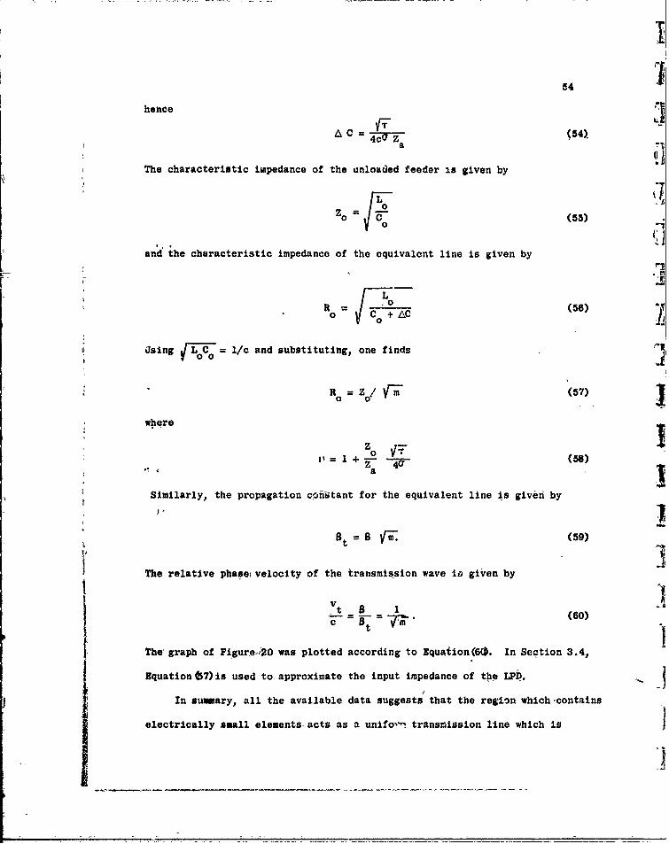
The' graph of Figure 20 was plotted according to Equation 60. In Section 3.4,

Equation (7)is used to approximate the input impedance of the LPD.

In sumary, all the available data suggests that the region which-contains

electrically small elements acts as a unifo,'' transmission line which is

I• 55

matched to the active region. This is why the front end of an IPD can -be

T truncated without adve r s e effects on the frequency independent character-

istics.

3.2 The Active Region

The active region .n-the LPD antenna consists of several dipole elements

whose lengths border on a half-wavelength at a given friquency, and the

4-portion of feeder to which these elements are attached. It is this part of

tbe antenna which determines the characteristics of the radiated field. This

section presents calculated and measured results whoch show how the power

Iin-the feeder wave is divided among the radiating elements. A useful concept,

the bandwidth of the active region, is formulated and its functional dependence

on the several LPD parameters is given.

3.2.1 Element Base Current in the Active-Region

The dipole elements in the active region transfer the power from

I the transmission wave to the radiated field. Figure 23 shows the base

impedances of the dipole elements in n 8-element LPD operating at f4 "

Base impedance here means the ratio of voltage to cirrent at the base

of each element, when the antenna is fed i'n the usual manner. The base

impedancea of elements 4 and 5 are predominately real, so conditions are

favorable for the coupling of energy from the feeder onto the radiating

elements in the active region. The small elements 6, 7, and 8 are capacitive

Land therefore loosely coupled to the feeder. The large elexe~nts 1, 2, and 3

are inductive and also Ioosell -y- oupled. The base impedance of all computed

models in -the range 0.8 <'T < 0.98 and 0.03 < U < 0.23 behaved in a

V similir manner. For T < 0.8, th6 base impedance of only one antenna

element was predominately real at any given frequency; for these models the

U. performance was not frequency independent.

2 ... . :2 ..

Im (Zb)

0'20 300

200

100

.3

200R e Zb),- 200 -100 100 200

"Q 5

'6

07o

-0200

8-0.

* Figure 23. Computed ho impedance Z vs. element number for an eightelement LPD at frequency 4

t4

567

Figure 24 is a graph of the relative amplitude of element base current

as a function ofWx/., Which is the normilized distance from the apex of the

antenna. The location of each element is indicated in the figure. The

lines which connect the values oZ current at the discrete location of each

j element are for clarity of presentation only. A loop-probe technique was

used to measure the base current, as explained in Appendix B. The element

base currents in the active region rise to a peak in the element which is

sovewhat shorter than a half-wavelength. As frequency is-chanCed, the shape

of this curve remains unchanged as shown Pn Figures J5, 26, 27 and 28. Thai.

f is, the active -region moves along the antenna as frequency is changed, but its

distance in wavelengths from the apex remains constant. Figure 29 shows the

computed magnitude of the base currents in the active region of an eight

element antenna at frequencies related by T. These curves are identical

except for f and f At these frequencies the active region becomes

deformed as it begins to include the largest or smallest element on the

antenna. When this happens, the lower or upper frequency limit is reached

1. The phase of the current from element to element in the active region

is also plotted in Figures 24 through 28. This is the phase which has to be

considered, when computing the radiation pattern. Since -the phase can be determined

only within a multiple of 2 , many phase -velocities are compatible with a

given phase progression. In Figures 24,through 28, the slope of the phase

curve in the active region was chosen to yield the largest phase velocity

compatible with the given phase progression. This phase velocity is approxibately,

equivalent to that of the first backward space harmonic of a periodic structure

made up of cells identical to the central cell of the active region. Mayes)17

Deschamps and Patton have explained the operation of unidirectional

If

58

+90

a

90'

I-,

-'5 II

=: -20 -

4/ /

+90 0 1.2_.

S-|80 "' -- V-- "- "

A~ MEASURED COMPUITE D 0

12-

0.70 0.0 0.0,.0 tI0 120O3

DISTANCE MHOM APEX-"

Figure 24, Computed and measured amplitude and phase of the nlementbase current vs. -relative distance from the apex, atfrequency f3; T = 0.95, a = 0.0564, Z = 109, h/a 177,Z, short circuit at h,/2.

'F 59L s

0

-5

a.

-0 -

U/

(n +90

w

o 0

uJ

wU + 90

a. fr / /-180 L 4

A MEASURED COMPUTED0

'2POSITION OF ELEMENTS .0

0,70 0.80 0.90 1.00 1.10 1.20 1.30

DISTANCE FROM APEXX~

Ftgure 25. Computed and measured amplitude and phase of the element base curentvs. relative distance from the apex, at frequency f3 " T f 0.95,0=0.05641 Z = 100, h/a 177, ZT = short circuit at~i2 .

60

0-

-5

z

o /

w

0

ISO

4

ww 0

U) -20~ +1801

/ //+9°0

'- /w -90 Q

A~ MEASURED COMPUTED-0

POSITION OF ELEMENTS1 1 _2 1 0 -I I , I - ,

0:70 o - eo 0.90 1.00 1.10 1.20 i.30

DISTANCEFROM APEX,

Figure 26. Computed and measured amplitude and phase of the element base current

vs. relative distance from the apex, at frequency f3 T 0.95,Q =-0.0564, Z = 100, h/a = 1773 ZOT short circuit 3a'R/2

0 1

0

-5 I

0

.- 0

a.Z

= -20o +180

: +90

w 0

UW 4-90- -' B .-

A MEASURED CO!i'UTEO 0

12PSITIO OF ELEMENTS%

ID0.70 0.80 0.90 1.00 1.10 1-.20 1.30DISTANCE FROM APEX

fi Figure 27. Computed and measured amplitude and phase of the-element base currentvs. relative distance from the apex, at frequency f3 0.95,

0.0564, Z 0 100, h/a O177, ZT short circuAM 1 /2.DITNEIRMAPXF

l

62 10-

O 0-5 /

zIuJ jO= -go -I '

wAc.

< " I-15 - 1

w

I. 0-20

i-180, I ,I

4 /I

0.70 0.80 0,90, 1.10 .. SO

DISTANCE. FROM -APEX

Figure 28. Computed and measured amplitude and phase of the element base current

Vo%/ relative distance from the apex, at frequency f 4; T =0.95Ja7 0.0564, Z° 0 100, h/a =177, ZT =short circuit at hl/2. "

i 00 1!

""I

I'63

II

w 1.0 -f 3 f 5 1

_J 0.9 -

,- 0.8 .

I =: 0.7 -

0.6

Ca 0.5- w

I- 0.4II -jU., 0.3,.

0.2

0.1

I 2 3 4 5 S

ELEMENT NUMBER

Figure.29. Relative -amplitude of base current in the active region vs. elementnumber, frequencies f thru f. T = 0.888, tr -O.089, N 8,Z 0 100, h/a = 125, 1T i hoft at h /2.

; 7 -

*I-

64

frequency independent antennas in terms of backward wave radiation.

The computed phase velocity of the first backward space harmonic as

a function of a is shown in Figure 30 for several values of T. These

curves represent average values taken over several frequencies. As the

spkcing increases, the phase velocity increases. For low values of T

thk relative phase velocity increases rapidly with increasing a, indicating

the possibility of radiation broadside to the antenna. Several models

have exhibited broadside radiation patterns; these ar discussed in Section 3.5.

! The mutual impedance of the elements in the active region plays a

fundamental role in determining the amplitude and phase of the element

currents. To, find if any of the mutual terms in the element impedance

matrix could be neglected, several tests were -made in which the range of

the mutual coupling was changed. If z is the mutual impedance betweenij

elpment i and element j, the range is given by the number Ii-J[. Thus

raige 0 means all mutual terms are zero, range 1 means all mutual terms

excepting ihose for adjacent elements are zero, etc, Limiting the mutual

effect to range 2 causes distortion of the computed patterns. The average

input impedance level remains about the same, but the input standing wave

ratio increases from its actual value for full range coupling. This means

that one must take into accouit interaction at range 3 or greater to

determine the relative excitation of each element.

3.2.2 Width and Location of the Active Region

For a given antenna, the usable bandwidth for frequency independent

operation depends on the relative distance the active region can move before

it becomes distorted by the smallest or largest element. Thus the width of

r(

!I65

1.7 UO.

i I ,.6-

I 1.5 -" T=0.8

1 1.4 -

S 1.3-

o 1.2

w x . T0.875

1.0 -

I-

f 0.8

> Q- 0.78

. -I L 0 .6 "C '0 1 9 2

! -0..,,T ~00.6

1I 0.5

0.3 -

0.1 -0 . ....... L...-...I..

" 0

0.04 0.06 ;0.08 0.10, 0.12 0.14 0.16 0.18 0.20 0.22 0.24

RELATIVE SPACING 0"

1 Figure 30. Computed relative phase velocity of the first backward spaceharmonic In the active region vs. U for several vilues of TZ 100- and h/a 177.

1. 0

iii

66

the active region, if proverly defined, can be used to measure the band-

width capbility of a given antenna. Furthermore, the knowledge of the

width of the active region is prerequisite to the design of an antenna

to cover a given bandwidth. The lower cut-off frequency of a given antenna

is determined by the length of the longest element. Conversely, if the

loser cut-off frequency is given, the relative length of the longest required

element in the active region must be known to fix the length of the

longest element on the antenna.

If the active region was very narrow, the operating -bandwidth of the

antenna would be given substantially by the ratio of the length of the

largest to smallest element. This ratio will be called the structure

bandwidth, B .

1 TI- (61)Bs =r-=N

Since the active region has some width, it is apparent that the operating

bandwidth B is always less than B by a factor which can be called the5

bandwidth of the active region, B Thusar

B = Bs/Bar. (62)

Placing numerical values on B and B is complicated by the fact that the~ar

width of the active region is not easily quantified. This is hicause the

observable characteristics of an LPD such as the pattern and input impedance

do not change abruptly from the values which characterize frequency independent

operation to, values'which are unquestionably outside the range of operation.

Actually, the characteristics change slowly, and only by applying a tolerance

to the pattern, or input impedance, can a figure be chosen which represents

the operating bandwidth of an LPD.

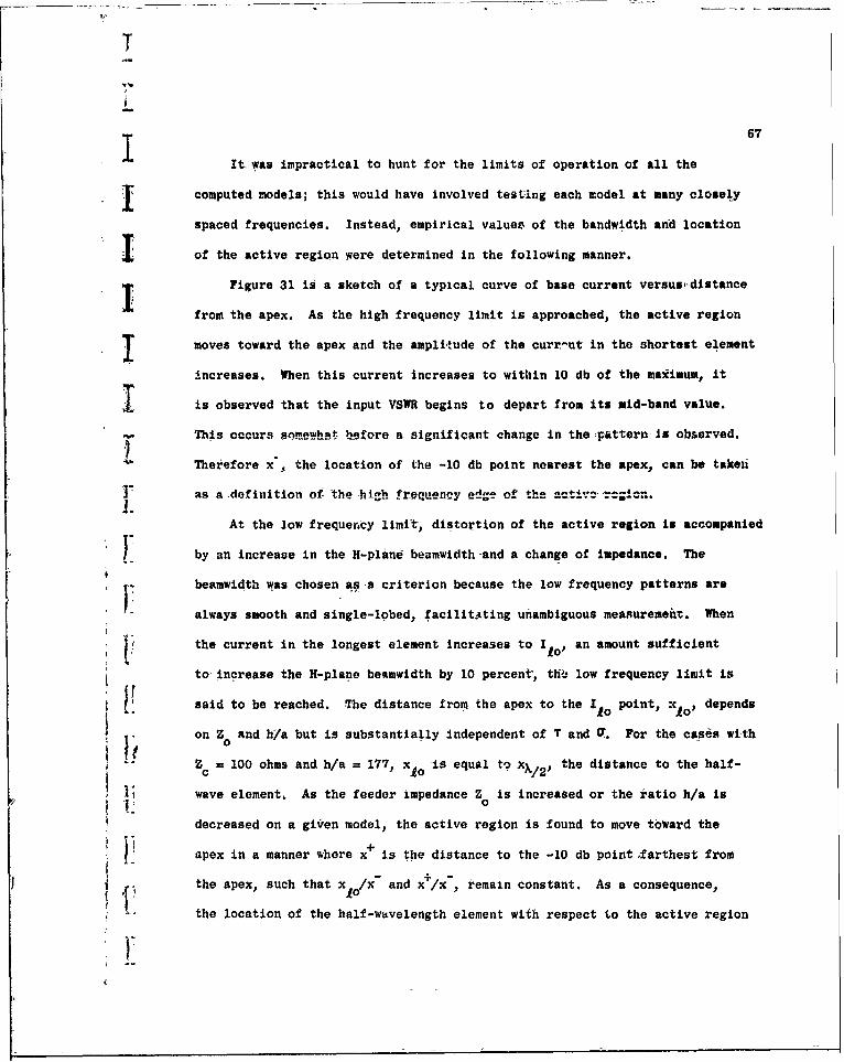
T

I67It was impractical to hunt for the limits of operation of all the

j computed models; this would have involved testing each model at many closely

spaced frequencies. Instead, empirical values of the bandwidth and location

of the active region were determined in the following manner.

i Figure 31 is a sketch of a typical curve of base current versus distance

from the apex. As the high frequency limit is approached, the active region

moves toward the apex and the amplitude of the curr-nt in the shortest element

increases. When this current increases to within 10 db of the maximum, it

I is observed that the input VSWR begins to depart from its mid-band value.

This occurs sov-ewhat before a- significant change in the =pattern s observed.

Therefore x', the location of the -10 db point nearest the apex, can be taken

as a definition of the -high -f requeney edge of the mactie -'rc.

At the low frequency limit, distortion of the active region is accompanied

by an increase in the -H-plane beamwidth -and a change of impedance. The

~beamwidth was chosen as-a criterion because the low frequency patterns are

always smooth and single-lobed, ;acilit-ating unambiguous measurement. When

the current in the longest element increases to I1 , an amount sufficient

to increase the H-plane beamwidth by 10 percent, th6 low frequency limit is

said to be reached. The distance from the apex to the 1 0 point, X1o1 depends

on Z and h/a but is substantially independent of T and O. For the cases with

Z = 100 ohms and h/a = 177, XAo is equal to xk/2 , the distance to the half-

wave element, As the feeder impedance Z is increased or the ratio h/a isV 0

decreased on a given model, the active region is found to move toward the

I +apex in a manner where x is the distance to the -10 db point farthest from

the apex, such that x /x and x+/x, remain constant. As a consequence,

the location of the half-wavelength element with respect to the active region

1'~

68

+.4

444

0

34 04.'

4A

0

4.'

w,

0.0Uw 0

4.

0 -PC~

0

U 4

0-09

T*4

'80~~ ~ ~ ~ 3ailWVI-48O3V

A

69

changes.

Knowing the high and low frequency edges of the active region, the band-

Twidth of the active region is given byx

Br (63)

In many practical applications the requirements will be less stringp.nt aid the

I bandwidth of the active region can be decreased'accordingly. In a previous

T papir was taken as the low frequency edge. The old-defLition was,

subsequently found to result in B Is gruater than ,iecessary for values ofar

T -less than 0.875. A graph of Bar versus a for several values of T -

shown in Figure 32. The circles are computed values and the strgitht 7A1es

are- iased, o an eiprical formula fitted to the computed results,

L Bar = 1.1 + 30.7 a(I-T) (64)

The empirical formula agrees with the computed and measured results for all

but the lowest values of T, jo its use should be restricted to T > C'875.

For a fixed T, the bandwidth of the active region increases as a increases.

This is an important design consideration, because the size of an antenna

V to cover a given bated increases as B increases.ar

The relationship between Io and xX/2 takes the form

x S(Z J. h/a) xX2(65)

Due to the geometry of the antenna, an identical relation exists between

the half-wavelength transverse dimension and the length of the largest

requirek e'emjnt in tkio active region.

10 S(Zo) h/a) (66)

K

70 'Ii

2,61 T=0.8

2.5 -0 COMPUTFD

2.4 - EMPIRICAL FORMULA

2.31-

2.2 0j

2.1 :1

r000w 2.0 o t0.875

10.92

-1.

o0I.? t 0.92

1.6 0 0--

1.5

1.1

0 .05 .10 .5 .20 .25

1o .ATIVE SPACING T "

Figure 3S2. Bandwidth of the active region, BarP vs. 0 and T.

F

'1 71j Thus S represents a shortening factor, and it serves to locate the active

region.with respect to the half-wavelength transverse dimension. Figure 33

is a graph of the computed shortening factor as a function of Z for several

values of 1/a. S was found to be essentially independent of T and O in the

range 0,1 < T < 0.95, and 0.075,< a <,0.2-. In the computed models, low

Jvalues ol h/a which correspond to thick elements were not extensivelyinvestigated; in these cases the approximations of the theory are not well

I satisfied. The curves have been extrapolated to 1 ,w values of h/a by the

inclusion of measured results. The S factor is significant; for high

values of feeder impedance the shortening can be equivalent to scaling the

antenna'by a factor T, resulting in the saving of one element at the large

end of the antenna. Work done by Isbell on models in which the radii

of the elements were held constant, so that h/a varied from 20 to 100,

showed that'the largest element was roughly 0.47X at the low frequency

cut-off, and this agrees with the trend observed in Figure 33. Another

19researcher in the field agrees with the location of the active region,

but finds that the stated values of B are somewhat high if the front,1 ar

to-back ratio of the pattern is used as a criterion- At any rate, the above

Fi results can be used as a guide in the design of LPD antennas for specific

applications.

L" 3.3 The Unexcited Region

The unexcited region consists of all dipr.Ae elements larger than a half-

'I wavelength at a given frequency, and the portion of feeder to which these

elements are attached. This section shows that an unexcited region exists

*on an LPD because of the efficient manner in which the power in the feeder

L, wave is radiated by the active region. In this case the operation of the LPD

antenna is unaffected by the truncation at the large end. The results of

I72,

1.10 . .-

1.08- COMPUTED

1.06 .... EXTRAPOLATED- FROM

EXPERIMENTAL DATA

1.04 j

1.00

0.98 1< 0.96 h/a 3

W 0.94I-0

cn 0.92-1

0.901-/ 3

b .10.8

0.86

0.84 F0.82 a o0:80 I ....I II

0 100 200 300 400 50

FEEDER IMPEDANCE Zo OHMS

Figure 33. Shortening- factor 8, vs. Zo and h/a.

t]

ii£

73

I several measurements of this property are presented.

Perhaps the most easily observed property of a successful log-periodic

I antenna is the insensitivity of the pattern and input impedance to the abrupt

discontinuity at the large end of the antenne between the structure and

free space. The absence of end effects can be verified by distorting the

Istructure at the large end of the antenna or by operating the antenna in

front of a conducting screen. In either case the characteristics of the antenna

performance should not change. This lack of end-eafect was observed by the

original researchers in .. field and was postulated as a necessary condition

for log-periodic performance. Furthermore, it was thought that a necessary

j-condition for lack of end effect was that the major portion-of the radiated

-field- should be in the direction of shorter elements, so that the longer

j elements are not illuminated,

-As shown in the preceding section, the magnitude of the element current

decreases rapidly in the unexcited region. This is because most of the

incident power in the transmission wave has been -radiated by the elements

of the active region. One might reason that the elements which are longer

than a half wavelength are not-efficiently coupled to the feeder, due to a

difference ii impedancc levels. This is true to an extent, but the fact remains

that on a successful LPD there is no-practical amount of power on the feeder

to excite the longer elements, even if they were efficiently coupled. In

fact, there do exist many regions where coupling is favorable; they are

in the neighborhood of elements whose lengths are odd multiples of a half-

wavelength. These regions will radiate if power is delivered to them by the

1. feeder. This-effect has been exploited by Professor Mayes and the author

in the design of high gain multi-mode LP antennas 20.

74,

The %mount of end effect or excitation of L-elements depends on the2T

radiating efficiency of the active region. Assuming the rest of the t

structure lossless, the radiating efficiency can be defined as

p. - Pq N T (67)?IN

P INs ,the total input power and PT is the power dissipated in n matched resistor

at the large end of the antenna, i.e. ZT =,Zo . End efect depends on the amount

of power delivered to the termination, and-one Would expect PT to be negligible "

when the antenna is performing satisfactorily. Figure-34 is a graph of 1 versus

the length of the longest element -in wavelengths. Computed values for feeder

impedances of 100 and 300 ohms are plotted for an LPD with T = 0.888 and

0 = 0.089. The relative length of the longest element was varied by changiilg

the frequency; identical results would obtain by changing the antenna size. IWhen the longest element is a half-wavelength, more than 80% of the incident

power has been dissipated by radiation from the active region. The antenna .1is more efficient for Z 300 ohms than for Z = 100 ohms for fixed /

This is partially the result of the movement of the-active region toward the ismaller elements as Z is increased, as was discussed in Section 3.2.2. The I

Xts -on- the graph correspond to values measured by Isbell on an LPD with

T= 0-89 and a = 0.0275, with Z = 104 ohms, The measured results agree with Ithe computcO results for Z = 100-ohms in the neighborhood of I1/A = 0.5.

This is an indication that the- low frequency edge of the active region remains

-fixedas 0 is changed, JThe end effect or the possibility of exciting :-/2 elements on an LPD

-depends on T and the feeder impedance Z. Figure 35 shows the computed j0d

I

1 100-95- ' Z. = 3 0 0 1 L

90 -Z, 100 A

85 "

80-

1 75 -

j 70-65

I _ 6S60zS2',v 55 -

W 50-9 /0 40

-

3530-

25 -

20- COMPUTED

15- x MEASURED-IiSBEL.)

-

0.3 0.4'_ 0 5 0.6

RELATIVE LENGTH OF LONGEST ELEMENT 1/A

Figure 34. Radiating efficiency of the active region vs. zelative length

Af the longest element.

I-- _______________________________ __ _______________ ___________________

76

N*

0

CY ZI' U,>V

000 U 1

cv 0

41CI

InIw OD'

% ~ ~ ~ ~ ~ A 0O30:4 N.VCV

JI

77

efficiency as a function of Z for T 0.92 and1/

and 1 1 A=0.71, and for T = 0.800 and 11/k = 0.97. The curves were doeermined

by averaging high, optimum, and low values of 0; the deviation ranges from

+ 3% for T 0.8 to+ 1% for T = 0.92. For the given values of A the

active region is ,well ahead of the longest element. Neyertheless for low

values of T and Z an apPreciable amount of power remains on the feeder behind0

theiantenna. If the efficiency is less than 85 or 90 percent and the antenna

is terminated in a mis-match (e.g. a short circuit), sufficient power will

be reflected back into the active region to cause the antenna characteristics

to depend on frequency. If an LPD has an operating bandwidth greater than

3:,, at soue frequencies 3X/2 elemdnts will exist on the antenna. If the

efficiency of this model is low the 3X/2 elements will be energized, and

there will be two active regions of the anteiina. In severe cases pattern

lobingk will occur.

Provided the efficiency is gieater than 90%, a short circuit at a distance

h /2 behind the longest element is a satisfactory termination for sll m6dels

in th6 range 0.8 T < 0.98 and-0.03- <'0.23. The 90% efficiency--requirement

places a lower limit on the allowable values of T and Z . This is why it is0

difficult to achieve, for example, a S0-ohm input impedance -if the required

feoder impedance is less than 75 ohms-and T is less than 0.888. The relation

between feeder impedance and input 'Impdance is discussed in Section 3.4.3.

The absence of end effect is an -important feature of frequency independent

gntennas. -t hac been found 4-thethe frequency dependent perfo-ianc0 of

H many unsuccessful log-periodfc structures can be attributed to end effects,

3.4 The Input Impedance

The input impedance of a log-periodic dipole antenna- is measured at the

78

juncture of the feeder and the smallest dipole element. This sectio. considers

0 the input impedance level as being determined primarily by the characteristics

of the equivalent line in the transmission region. Dta are presented which

show how the input impedance depends on the -arious LPD parameters, and an

approximate formula is given which enables one to design an LPD with a

required input impedance. A wide practical range of impedance levels can

be obtained, and factors which ultimately limit this rangeare discusedi

34.1 General Characteristics of LPD Input Impedaice-I

A plot of input impedance versus frequency for an, eight element LPD

with T = 0.888 ,andzU = 0.089 is shown on the Smith Chart of Figure 36. The

nuibers on-the chart are the J's in -

=f 1 T, 1 (68)

-whire f is the frequency for which element 1i s a--half-wavelength long.

Except for ff 1/ 2 , f 7 and f8 the points cluster around a mean-resistance

level R " To find Ro a circle is drawn with its center on the resistance

axis, enclosingthe cluster. The intersections of the circle with the resistance

axis determines the minimum and maximum swing of resistance. P Is then given

1 by-byi 7 (69)

i 'R0 = JRma x R '-in' 89

The standiii- -ave ratio-with revpect to Re is given by

ntgure 36 the-mean resistance level is 72-ohms and the standingwave ratio,

-wih respect toh ms, is 1.25:1. The points for f and f1/2 fall outside I-

------------ ---/ _ __

79

iid

'4

Alr

the cluster; this 4ndicates that the low frequency limit has been exceeded.

The points f7 and f8 also fall outside the cluster, indicating that the

high frequency limit has been exceeded. These effects are typical and char-

acterize all LP arlennas. To the extent that the SWR can be neglected the

points which make up the cluster define the frequency independent impedance

bndwidth of this antenna.

Ideally, the input impedance at the apex of an infinite log-periodic

structure should- be the same for all frequencies rel'ted by the scale factor

T. There is at least one reason why this does not generally hold for LP

antennas, even ,for frequencies within the design band. In any .:xactical LP,

the scaling from cell to cell must start at a small but finite element, because

'the device which, delivers energy to the antenna cannot be made arbitrarily

small. This means that there is always a portion of the strvcture missing

'.due to the front truncation. Ii Section 3.1 it was shown that the transmission

region acts as a uniform line. Since a fixed- length of this line is missing

i(the part from the apex to the smallest element), impedances are not trans- ,

formed to the apex, and a frequency dependent variation is imposed. The

departure from the ideal log-periodic variation is negligible only if the

removed piece of line is electrically small at the ijighest operating frequencies.

The electrical length of front-truncated line depends on the propagation constant

in -the transmission -egion and the distance x N from the apex to the shortest Uelement. In some cases the front truncation can introduce an appreciable

effect. The~graph of Figure 36 is one such example. Here the equivalent

length of theb-iont truncativit-amounts to 0.75X t at the high frequency limit

(t is,the *avelength of the tiazismission wave). The input impedances at

frequencies relatedby integral powers of are not equal. An example of

- .-- .:- - - - - -- - - --

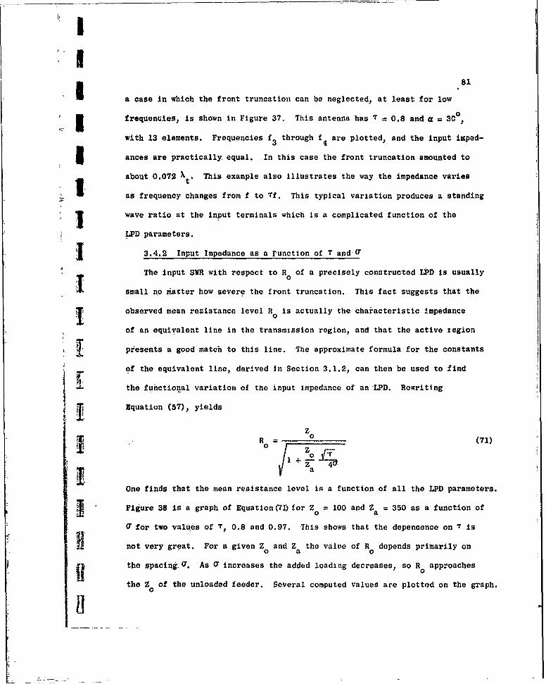
* 81

- a case in which the front truncatioa can be neglected, at least for low

:. 3 frequencies, is shown in Figure 37. This antenna has T = 0.8 and 1 = 3C0 ,

with 13 elements. Frequencies f3 through f4 are plotted, and the input isped-

5 ances are practically equal. In this case the front truncation amounted to

about 0.072 %t. This example also Illustrates the way the impedance varies

as frequency changes from f to Tf. This typical variation produces a standing

wave ratio at the input terminals which is a complicated function of the

LPD parameters.

1 3.4.2 Input Impedance as a Function of T and-a

The input SWR with respect to R of a precisely constructed LPD is usually

small no matter how severe the front truncation. This fact suggests that the

observed mean resistance level R0 is actually the characteristic impedance

of an equivalent line in the transmission region, and that the active legion

presents a good-match to this line. The approximate formula for the constants

of the equivalent line, derived In Section 3.1.2, can then be used to find

the functional variation of the input impedance of an LPD. Rewriting

Equation (57), yields

zRo 0 (71)

1 Za 4O

One finds that the mean resistance level is a function of all the LPD parameters.

Figure 38 is a graph of Equation(7]) for Z 0 100 and Z = 350 as a function of

O for two values of T, 0.8 and 0.97. This shows that the depenaence on T is

not very great. For a given Z and Z the value of R depends primarily ono a o

the spacingia. As a increases the added loading decreases, so R approaches0

the Z of the unloaded feeder. Several computed values are plottod on the graph.0

82

41

it:

V3

I83

3 0

90-

1 85r x

ex

SC P80.

T 00 75

Lx

65

0.04 0.08 0.12 0.16 0.20 0.24 0.28

RELATIVE SPACING (7

Figure 38. Input impedance R vs. 01 and T for Z 0 100 and h/a 177.

.

84

The errcr between the approximate furmula and measured or computed results

is usually less than 10%.

An indication of the nature of the- error involved in assuming that the

capacitive loading of a small element is distributed-uniformly over a section

of the feeder can be found. Consider the loading to consist of small, 3identical elements, uniformly spaced. -Assuming the capacitanco of a small

dipole to be proportional to its length a- in Section 311.2, the characteristic

impedance of this-equivalent line can-be fovund. It 13

ZRo _o (72)

0 T

-P

+ ~ a-7.91n i+ - a (P (Cos (- 1) "

a21rd

Here 9'-is the electrical length in-radians of one section of line. 9 ="--,

where d -is the distance-between -neighboring elements. As 9Vgoes to zero

(72) reduces to (71). A graph of the error involved in using (71) rather

than (72) is ishown in Figure-39, where the percent error is plotted -as a

function-of 41X. The error is- small for -all values oT d/X found in -the

transmission region of an LPD.

The computed standing wave -ratio with respect to R- as a function of aA0

for several vsaues of T is shown-in Figure 40. For these-models Z = 100 ohms 3and h/a = 177. The SWR decreases as T increases, and for low values of T, a

minimum value of SWR-exists. For the two large laboratory models which were jused for the -near field measurements, the values of SWR agreed with the

computed values. However, the SWR of pattern models was always greater than

KI85I

II

10 k 2.0

9

1 70 6 -

n- 5- k z "

0 IO 4 k=1.0

4K

II

0 0.01 0.02 0.03 0.04 0,05 o. 6 0.07 0.08 0.09 0.10

DISTANCE BETWEEN ELEMENTS d/X

Figure 39. Difference between the approximate discrete formula andapproximate distributed formula for R , vs. the distancebetwoor elenents as a percent of the atter.

LIi -L

(11'

?6i I

2.0

01.9

01.8

1.7U

: T= 0.7

o 1.5

1.4

1.3 -3z

z 1.2 t

LIlI.I - "T=0.95 r

1.0 I I I -I0.04 0.06 0.08 0.10 0.12 0.34 0.16 0.18 0.20 0.22 0.24 13

RELATIVE 3SPACING T"

Figure 40, Computed SIYR vs. 0 and T. for Z = 100 and h/a = 177.

87

U the computed value; this is because tho details of the feed-point geometry

assume additional importance at higher frequencies.

3.4.3 Input Impedance as a Function of Z and h/sI 0

I For fixed T and O, the mean resistance level is determined by the chcracteristic

Impedance of the feeder, Zo . The graph of Figure 41 shows that R increases

as Z increases. The computed points are shown along with the measured values.

IIn addition) points calculated from the approximatc formula (71) are also

shown. In all cases the agreement is good, demonstrating the utility of

I the approximate formula.

Figure 42 shows how -R depends on Z as a- function of the mean- spacing0 0

factor U' = iVT using the approximate formula (71). As 0 increases,

the slope of the curves approach unity, indicating that R approaches-Z

The element thickness as given by the ratio h/a can also be used to control

1the input impedance. Figure 43 s:iows the effect of changing h/a with fixed

Zo, for aeveral values of O . As h/a increases, the loading decreases and

R increases.0

LIt can be seen from the preceding graphs that the input impedance of

I.PD antennas can be adjusted over a wide range. The upper limit is determined

Vby the problems involved in constructing feeder configurations. Even when

four wire balanced lines are used, characteristic impedances greater than

600 ohms are difficult to achieve. An added reactance due to the large gap

between the two halves of each dipole would possibly cause detrimental effects.

In the computed models there was no way of taking this into account; the computer

results show that antennas with Z = 500 ohms work just as well as antennas0

with Z = 100 ohms. The lower limit of Z is determined by the radiatingI: ° °

0

N 1.4-1.3 X

V) x

100 I0

o 1w 80 Xu. I- 60

0z

40tI

-0--*- CALCULATEDz XXXX EXPERIMENTAL jw 30 -0--- APPROXIMATE FORMULA

. I I.- II

30 50 7o 90 110 130 -150.

FEEDER IMPEDANCE Z*OHMS-

Figure 43. Input impedance R° vs. feeder impedance Z, T 0.888,Or 0.089, N = 5, h/a 125.

89

:1 300

1 250

200

0

100-4 ~50 I

50 100 150 200 250 300

Figurc 42. Input imipedance RO vs. ZO and a'with h/a =177, from the approximateformula. 0

90

S-i 06 0 6

b b b

cc C

o

o 0oSINH *N ONV0dVYIindN

91

efficiency of the antenna. As previoualy shown in Secticn 3.3, in all models

I in which Z is less than 75 ohms an appreciable amount of power remains on

the feeder at the large end of the-antenna. This power is reflected back through

the antenna if the feeder is shorted at the large end, as is commonly done,

or it ji wasted if a resistive terminatiop is used. This effect has been

Ldetected in the cumputed models. Figure 44a shows the input impedance of

an LPD- witZ w 6G ohms, terminated -in a- 50 ohm resistor. The impedance

00locus.-has the same characteristics as foi higher va.lues of Zo . However,

: wheh a purely reactive termination is used, the input impedance locus

blossoms out as shown in Figure 44b, indicattng that the end effect is

appr6iable.. In addition, irregularitites in the pattern occur, -otherwise

11 the -increased SWR could probably be tolerated.

Formula (71) can be inverted to find the feeder impedance required to,

achieve a given input impedance. In its most useful form Z is normalized0

with respect to R, resulting in

0

1:o _ 1 3.iS Za ° + - 1 .(73)

ano[0As in Iquation (71) Za is the average characteristic impedance of a short

- dipole) given by

Za = 120 (in h/a - 2.25). (74)

A graph of Za versus h/a is given in Figure 45. Figure 46 is a graph of the

V relative feeder impedance Z a/RO versus the relative characteristic dipole0impedance Za/Ro, for several values of the mean spacing factor This graph

/

can-be used to design for a specific input impedance, given O and Za

921

010

a

S

4J0

* -4.,-, ~ -- . o

f4.

1 93

4

64, 0

jII

1+

- b

K ~ V ~ 4J

.V

94

In 44

4 3

A

N WYz

cuU

a be______-.4co

$48 8- 0- 0000 9ODI0 n I

VZ _1dO1-3 C3~ -IS81VUV33V3V

NbI- P4

95.

1 02

.

.9- 0L ~Cn

VM

00

cr 40

II :

96

Input impedance levels from 35 to 200 ohms have been measured using the

coaxial lhne feed method pictured in Figure 9. If higher impedance levels

are -required for use with balanced twin line, the 4:1 balun transformer

scheme suggested by Dr. Jordan can be used. In figure 47, the feeder of

an LlAD is shown but thW elements are not. 'I represents the antenna input

impedance at the front end. This load can be driven in parallel by two

-coaxial lines of characteristic impedance 2R . Each line is inserted through

i one of the feeders as shown, and at the back of the a.itenna they are connected

in series. A parallel wire line with characteristic impedance 4R, is then

-connected to the series combination, resulting in a perfect match to the

antenna. This balun transformer -scheme has a bandwidth. q'il to the operating

-bandwidth of the antenna. Since there is no current ,on the--feeder at the

-back of the antenna, the quarter-wLve choke which is-ordinarily used in a

4-4:1 balun is not required,. so the balun does not depend on frequency. This

-technique has been used with success in the design-of LPD television receiving

:antennas. ,

3.5 The Far Field Radiation

The far field properties of the LP1D antenna are determined from the

- 'equations of Section 2.2.2. This section presents' computed -results which show

: how th'e characteristic pattern of an LPD depenids on the various parameters.

The charact ristic pattern of an LPD is defined as the pattern which typifies

the )ntenna for all frequencies within the aesitn band. The cnmputed patterns-.are-eompared-with ptternt bf several expiormental models,-recorded by the i

:University of Illinois Antenna Laboratory pattern range facilities.

'Consideratibn is also. given to factors which control the relative phase of

the far f1 ld. The phase center of an LPD is defined, -and measured and computed

I97

'I -~ 4.

4'o coo

.1 Z Nz Ila

0 IIIILI 0

U II II z

1T -1 z

I II Iw .-

II zI

II - -I ~ ,.

I III

I--

I I JN

-o vz

t

0 -M

2 0 l a12 Z I

ILL.

T

98

data are presented which show that the phase center is located at the active

region. [3.5.1 Radiation Patterns

-Examples of the computed relative field intensity patterns are shown Iin Figure 48. For this LPD, T = 0.888, 9 = 0.089 and- N = 8, fj denotes the Ufrequency

f j = f (5) 'l0

,where f1 is the frequency for which element number one is a half-wavelength-

long. The characteristic pattern is, observed over the range fI to f7, which

yields- a pattern bandwidth of approximately (0.888) = 2-04. At f8 definite

pattern deterioration has occurred, indicating that tne high frequency limit

has been exceeded. Figures 53, 54, and 55a are enlarged patterns which sn 2

the negligible variation as frequency changes from f to Tf. The computed

patterns of Figure 49 are for the same antenna with fewer elements, N = 5.

Again there is no measurable difference. In addition to exhibiting negligible

variation over a period, the characteristic pattern of this antenna does

not depend 4onte nw*erof elements, as long as there are enough elements

to support the active region. Thus, according to the definition, this antenna

can be called frequency independent with respect to its radiation pattern.

This behavior is' typicafl of computed and measured -LPD patterns. The only IexceptIons occur when there is an and effect. These exceptions 4re char-

jcterized by petter~ie which ,change with frequency. The patterns broaden

and sometimes side lobes appear.

Thogross pattern behavior can be observed from a plot of the computed

hal f-pwer.beamw idth versus frequency, as in Figure 50. The E-plane pattern

-holds constant over a wider frequency range than the H-plane pattern.

99

I E- PLANE E- PLANE

-H- PLANE H- PLANE

- E--PLANE E- PLANEIff

I j!k 4, H-PLANE -H-PLANE

E- -PLANE E-PLANEf4 6 f

H- PLANE . H- PLANE

. f4 I * f8

i :H - PLANE H --- AN

I4-H -PLANE - H- PLANE

Figure 48. An example of radiation patterns computpd by ILLIAC,T= 0.883 (7 = .089 N = 8, Zo = 100, ZT short at

1h1/2

i f

100 -

f2__ NX58 N=' -

E -PiA E -H-LN

---- CMPUTE

i ur49 Copue patrs] .8,-9-C.8,z z1

Z _= shr th1/,soigIdfeec eweItrn for N 5In N

I

101

180

170

160

150

I 140

130

t, 120

or 80

C3

0 70

<J -r- E- PLANExZ 50 -

1- 40

30

20

1. 10

LOGARITHM OF FREQUENCY

Figure 50. Computed half Power b-m---dth vs. frequency; T 0.888, a 0.089,N 8, Z 0 0S , Z = short at hl/2.

0 T0

102

This trend is evidenced by all LPD antennas, and- results from the strong 1dependence of the H-plane pattern on the array factor of the antenna, whereas

the more directive E-plane element pattern masks small changes in the array

1factor. The graph of H-plane beamwidth shows that the active region spans

several elements, because the pattern bandwidth is significantly less than

the structure bandwidth. The graph also shows that -the center of the active

region is located somewhat ahead of the half-wavelength element, because

-the center of the .pattern band is located at a lower Irequency than the

center of the structure band. -'

Examples of measured and computed patterns are given in Figures 51 through

156 for T =O.888 and O = 0.089; in Figures 57 through 59 for T =-0.98 and

= 0.057, and in Figures 60 through 62 for T =0.8 andU =-0.137. The

:measured cross polarization was found to be more than 20- db below the

pattern maximum as long as the sp~cing between the -eeder conductors is small

4compared to the shortest wavelength of operation. In every case the computed

RE-plane beamwidth is narrower than the one measured, and the-computed H-plane

;beamwidth is wider than the one measured. Thes^ errors -tend to compensate each

: other in the computation of antenna directivity, so the comparison of computed

'and measured directi'&Aty Is more accurate than the comparison of computed j

and measured beamwidth. The error is incurred because the actual current

on the dipole elements apparently departs from the assumed sinusoidal form.

Actually, it can be seen from Equations (46) and (47) that the pattern

cannot 'be expressed as the product of an element factor and an array factor,because of the differing element lengths. However, it is convenient to thinkin these terms here, owing to tfe dissmilarity between the E-plane patternof a single element (a figure eight pattern) and the H-plane pattern(omnidirectional).

t.i

3 103

/II4

Io 1

-PLNH-PL ECOPUE MESUE

Fiur 51 optdadmauedpten;T=/801 .8,V,=10,Z hr th/

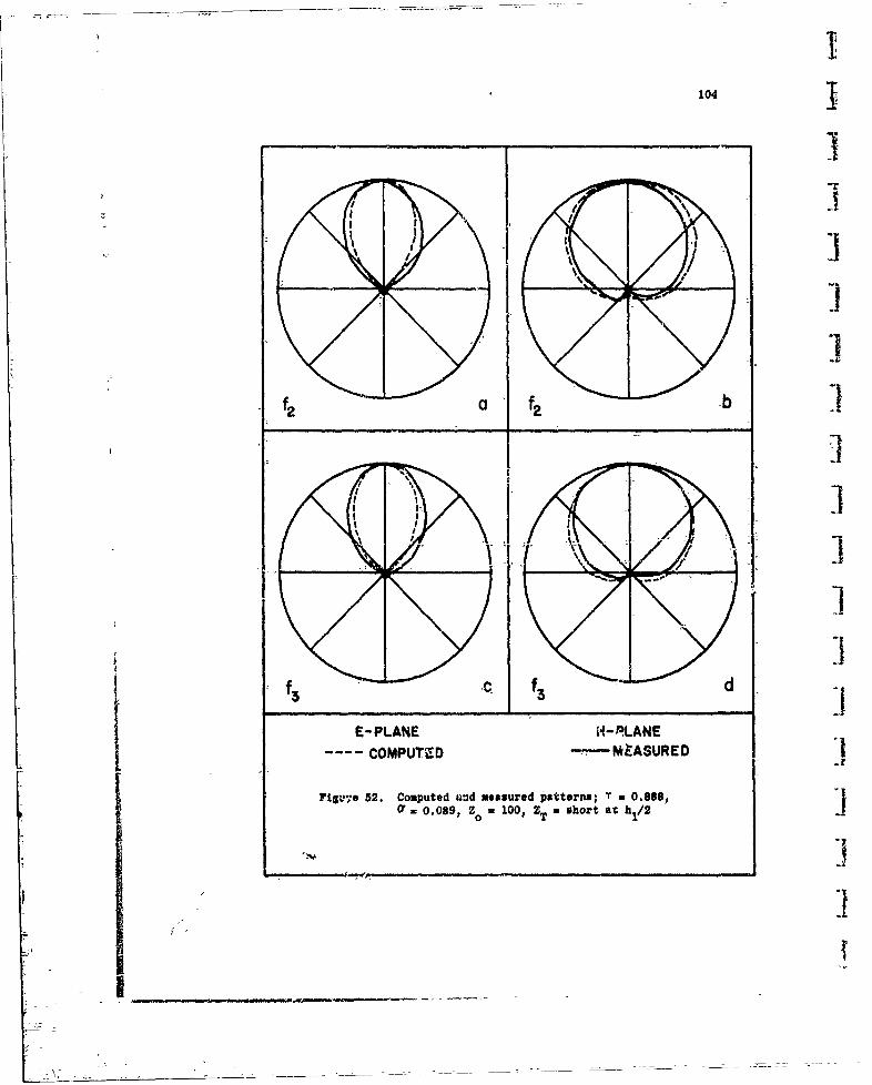
1041

f2 f2

f3 f3

E-PLANER-PLAN

COMPTED - -MZAUREFig~e 2.Comutd ud easre patens;T 0.88

01. .089 zo 00, T shrt a b11

3 105

II

1 4

--E-PLANE H -PLANECOMPUTED - MEASURED

Figure 53. Computed and measured patterns; T =-0.888,or=0.0Oi), Z 0 = 100, ZT = short at h/

106j

f1l f I b--

\~ f/1 A

-E-PLNE HPLA2

COMPUED -MASUREFigue 54 Copute andmeauredpattrns T 0888or 009,ZO 10)Z sor t /.

I 07,

I 41

f5 a__f5__b

E-PLANE H-PLANE

---- COMPUTED -MEASURED

Figure 55. Computed and measured patterns; T = 0.888,01=0.089, o -100, Z -shor th/

108j

av%

f7 47I

I5 ' C f

E-L N -L N

--- COPTEEAUE

Fi ur 5 / optd ad mauedpt en;T=os0.089 z -00, , shrt a hi/

1 109

4 4

E-LNEHPLNr OPTD MAUEFiue5.Cmue n esrdpten;T=09I0=007NI2 o 10 T hr th/

110

f~l 31

Figure 58. Computed and measured patterns; T = 0.98, 0' = 0.057) [N 12, ZO 0 100, ZT short at- 1 /2

I!

I A +I

LI I

/+

I11

I ,

I - - 1

!7/

* E-LN -LN

COPTDI EAUE

" iue5.Cmue n esrd atrs ":09aO .007* 2 0 =10 T =sota;h/

U /

I

'I-

112

4A

E-PLANE H- PLANECOMPUTED -MEASURED

Figure 60. Computed and measured patterns; T 0.8, Or 0.137,N =8, Z 100, ZT short at h/

.11

f 313

0- T

114

II J

ii

f4 a f4b

E-PLANE H-PLANE

COMPUTED - MEASURED

Figure 62. Computed and measured patterns; T = 0.8, O = 0.137,

N =8, Z0 100, ZT short at h /2

tII

- I

1115

I It can be shown that the E-plane pattern of a half-wave dipole antenna becomes

narrower as the current distribution changes from sinusoidal to uniform.

Thus the actual current distribution in the elements must be more nearly

uniform than-sinusoidal.

1 3.5.1.1 The Characteristic Pattern as a-Function of T and 9

I The scale factor T and the relative spacingaexercise: primary control

over the shape of the radiation patterns of LPD antennas. Figures -63 and

64 are plots of the computed E- and H-plane half pover beamwidth as a function

of (7 for several values of T. In -these curves Z = 100 ohms and h/a = 177.

Each-curve possccces a minimum in the range.0.12 < a < 0.18. ThIe H-plane

L beamwidth varies more than the E-plane beamwidth; it. should-be-noted chat

the scale of the ordinate is different in the two figures.

L Using the graphs of -Figures 63 and 64, tne directivity in decibels can

be approximated-using the formula from Kraus,21

41253

D 10 log 415 (76)(BWE ) (BW )BH

BW and BWH are the half-power beamwidths, In degrees. In Figure. 65 are

plotted contours of constant directivity in decibels, as a function of T

7 and 0. A scale for the angle a is also given. A straight line connecting

equal a indices on the top (or right) and the bottom edges of the graph

17. describes combinations of T and U corresponding to the given angle a.

All values of T and C which result in single-lobed frequency independent

patterns fall within this graph. For O less than 0;05- the directivity falls

off rapidly and the front to back ratio decreases. Values of T greater than

0.98 on the left side of Figure 65 have not been extensively Investigated,

zI116

t-DJ 60

58

,I t .87554-

WL!

w 52

4-.j .92 I

"1' :.95 (J 38

.4.06 .08 10 12 14 .16 .18 .20 .22 24 .26 :11

RELATIVE SPACING O3-

Flgutre 63. C omputed N-plane half-power boamwldth vs. T and 0";

Zo:l0,Z = short at hl/2, h/a =177.

00a.r

117

190

J 180

n170woD 160-

01

I 140

13 -w 'C = .875

w 1200k

U. 110 -

l100w0 .92

X 80 t 9

70 = .95

60-

.04 .06 .08 .10 .12 .14 .16 .18 .20 .22 .24 26ARELATIVE SPACING G

I Figure 64. Computed H-plane half-power boamwidth vs. T and Or;

Z= 100, ZT = short at hl/2, h/a = 177.

It

I

A70

118

% I I V11

14, P..

liti

"Plil IT1J

TX~

7i 1 0

N~~ l!0 0 0

21 01TVd RAI±Vlt1CN

119

3 because the number of elements required to achieve a given bandwidth becomec

excessive. Por values of C greater than the optimum (, the directivity falls

off and the patterns either tend toward broadside or side lobes appear. In

addition, the length of the antenna for a required bandwidth becomes excessive.

For T less than 0.8, only one dipole is near resonance at a given frequency,

I° and it couples an insufficient amount of energy from the feeder, resulting

in end effects which destroy the log;.periodic performance. Measured patterns

of such an antenna are shown its Figure 66, For this antenna T = 0.7 and

J a = 0.206. The feeder was terminated Ly an open circuit -at the largest

elemant. The patterns definitely depend on Lr£xten2y, one pattern has its

I maximum in the opposite direction. Terminating the feeder in a matched

T resistor resulted in the measured and computed H-plane patterns of Figure 67.

In-chis case the patterns are more nearly independent of frequency; however,

the addition of the matched termination has lowered the computed efficiency

to 70%. The patterns of Figure 67 also illustrate the broadside tendency

I_ which is characteristic of values of U much greater than the optimum.

The front-t.-back ratio as a function of T and a is shown in Figure 68.

-For T > 0-.875 the calculated F/B is greater than 20 db. The F/B f~r T < 0.875

depends on the value of 0; it attains a maximum for O near the optimum value

shown in Figure 65. F/B decreases as the cut-off frequencies are approached.

(Compare the patterns of Figures 51 through 56.) This decrease can be limited

to some exte.t by adjusting the reactive determination ZT. Isbell found that

6 short circuit at a distance h /2 behind the largest element resulted in

a minimum-deviation of F/B from its mid-band value.

3.5.1.2 The Characteristic Pattern as a Function of Z and h/a0

The computed and measvred patterns of an LPD with T = 0.888, O = 0.089,

1" and Z = 150 ohms are shown in -Figures 69 and 70. A comparison of the

corresponding patterns of Figures 52, 53, and 55, for Z= 100 ohms shows

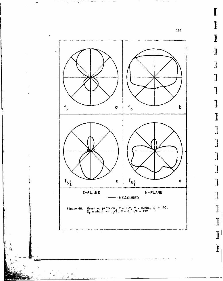
IIiI

120

r I

f3a f 3-3

i

3 3-1

E-PLANE H- PLANE---- MEASURED 21

Figure 66. Measured patterns; 7 = 0.7, 0.206, Z 0 100,

T = short at h 1 /2) N = 6, h/a = 77

___

j 39

- -- j" ¢ .' _ . .

121

I~ A

433I

I4

H-PLANE H-PLANE

--- COMPUTED -- MEASURED

Figure 67. Computed and measured fl-plane patterns; T = 0.7,

or~0 0.206, Z0 = 100, Z,= 100, N 6, b/a =177.

122

18 O IS16

00

0

S 12

o

P 14

I-z0

U.10 -

8 ]

6]6 I ,. I IU I ,I I I

0.06 0.08 0.10 0.2 0.14 0.16 0.18 0.20 0.22 1RELATIVE SPACING, O"

Fieure 68. Computed pattern front to back ratio vs. 0* and T;Z6 = 100, ZT = short at hl/2

123

-E 'L N H'- PL N

--- COMPUTED -MEASURED

Figur 69.computed-and meas~.red-patterns; T = 0.888,

Figure = 69 -0O.89, Z0 = 150, ZT u 1orah/

124

f5 a

E-LN - PLN

---- COMPUTED -MEASURED 4Figure 70. Computed and measured patterns; T =0.888,

a 0.089, z IS0, ZT -short at h.212UI0

125

m that a change in Z has little effect on the characteristic patterns.

In this model the average directivity decreased by less than one decibel is

the feeder impedance increased from 75 to 300 ohms. On nine models with

different T and 01, similar -results were observed; antennas with 0 greater.

than optimum lost as much as one db over th\ range 100 < Z < 300. For

1siall a the variation was less than O;5-db. As an approximation' suitable

for design purposes, one may assume that the diretivitycontours ofT Figure 65 hold for all practical values of Z

0

The-element thickness controls the directivity to some extent. Figure

71 shows that the average directivity decreases as the element height to radius

ratio increases. For this model, with T - 0 888oand ' =-O089, thq<decrease

amounts -to about 1.2 db over the range 100 < na < 1001000, Although the'

japproximations of the theory are best sattsried with large h/a, in thefrequency range for which -the Antenna Laboratory is equipped, it was imissible

to build models with h/a much greater than 800. Tne two laboratory models

T with T = 0.888 and a 0 0.089 agree with the trend-of tne curve for h/a < 800,

although -the measured directivity was low. As with Zo, the -variation seems'0I insignificant in the light of the approximations made, and for design purposes

the directivity contours of Figure 65 can be used if a small correction is-

- applied.

It has been found (.hat a-deprture from -the exact scaling, of the diameter

of each element can be tolerated If the dcameters of the elements are held-

L cnsfant, the directivity should increase with frequency. This increase was

riot observed in the laboratory models which covered a 3:1 bandwidth, because

11 other minor pattern variations masked the sought after trend. It is to be

expectod that the input VSWR wi-I1 increase if constant diameter elements are

used.

126

00

0~0

100

C4o 0 co 4 tNK .. i

'Sa~~ oIA~tPW

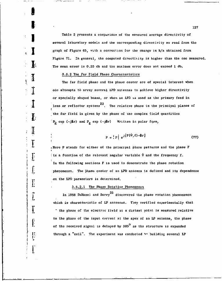
I

1 127

Table 2 presents a comparlson of the measured average directivity of

several laboratory models and the corresponding directivity as read from the

graph of Figure 65, with a correction for the change in h/a obtained from

Figure 71. In general, the computed directivity is higher than the one measured.

The mean error is 0.35 db and the maximum error does not exceed 1 db.

13.5.2 The Far Field Phase CharacteristicsThe far field phase and the phaue center are of special interest when

*I ione ,attempts to array several LPD antennas to achieve higher directivity

or specially shaped beams, or when an LPD i& used as the primary feed in

1 22lens or reflector systems . The relative phase in the principal planes of

the far field is given by the phase of the complex field quantities

P- exp (-Jar)- and P exp (-jBr) Written in polar form,

I P = !Pi eJ[F(4',f)-Br] (77)

,Here P stands for either of the principal plane patterns and the phase F

V iis a fAinction of the relevant angular variable ' and the frequency f.

In the following sections F is used to demonstrate the phase rotation

phenomenon. The phase center of an LPD antenna is defined and its dependence

on the LPD parameters is determined.

E3.5.2.1 The Phase Rotation Phenomenon

) In 1958 DuHamel and Berry2 3 discovered the phase rotation phenomenon

which is characteristic of LP antennas. T*Jey verified experimentally that

-_ the phase of the electric field at a distant point is measured relative

to the phase of the input current at the apex of an LP antenna the phase

'1 of the received signal is delayed by 3600 as the structure is expanded

through a "cell". The experiment was conducted ' building several LP

f ;.

'I

128

TABLE 2

Comparison-of keasurod and Conputed Directivity -.

Measured Computed

T,. Z 0/a BE BW D D

-0.98 0.057 5.0 100 125 56.5 85.7 9.31 10.0

0.98 0.038 7.5 75 240/148* 5e.1 85.7 9.50 9.50.975 C.0717 5.0 100 200/151* 52.8 76;6 10.08 10.0

0.95 0.0268 25.0 100 100/26* 68.7 114.2 7.20

0.93 0.125 8.0 65 66 60.0 85.0 9.08 9.8

0.92 0.200 5.7 100 142 52.7 69.1 10.53 9.9

0.92 0.160 7.1 100 177 57.0 80.2 9.56 10.0

0.92 0.150 7.6 300 60/20* 54.0- 85.4 9.53 9.8

0.92 0.120 9.5 100 118 57.0 81,1 9.52 9.4

0.92 0.080 14.0 100 177 61.5 98.0 8.36 8.9

0.91 0.128 10.0 94 06 59.2 90.8 8.85 9.4 10.89 0.103 15.0 75 80/45* 67.0 106.3 7.68 8.6

0.888 0.089 17.5 100 80 61.8 101.9 8.18 8.7

0.888 0.089 17.5 100 177 63.4 106.6 7.86 8.5

0.888 0.089 17.5 150 177 65.2 112.0 7.52 8.3

0.86 0.080 23.6 200 50 64.3 112 4 7.57 7.9

0.85 0.26 10.0 75 80/49* 71.3 10O 7.14 7.3 II0.84 0.068 30.5 215 50 67.8 164. 6.83 7.5

0.81 0.364 7.5 75 80/43* 95.0 180.0 3.83 ...

0.80- 0.137 20.0 100 125 58.5 101.9 8.41 8.3

* In tbeo models, the element diameter was hold constant; the h/t of the longestand shortest-element Is recorded.

!

I ., 129

,antennas with indentical T and a, the models differing from each other

in size. If Kx is the distance from the apex of the structure to element n,n

£s the expansion factor for each antenna is determined by assigning values

of K from 1 to 1/72. (The "cell" scaling factor for LPD antennas is T2

All other dimensions of the structure are also multiplied by K,

I Since an expansion of a log-periodic structure is equivalent to a-

change of frequency, the-phase rotation phenomenon can also be observed by

1 I measuring the phase of a given antenna as frequency is -increased from

f to f/T 2 provided that the distance r from the apex to the far field

point is decreased from -r to T 2r. The phase of a far field component is

given by the-exponent of Equation (77), F( ,f)-Br. Under the stated conditions

Br is held constant. The phase should-be measured relative to the input -,

I current at the apex of the antenna- so the front truncation which occurs

on most practical antennas must -be taken into acccunt for the reasons

Tgiven in Section 3.1.1. The dotted curve of Figure 72 is for a computed

model with T = 0.875 and-a = 0.067, from frequency f2 to f In this

2 4)1!model the front truncation was 0.158X at f2 and 0.206k at f 4 , ana the

computed values of F were corrected accordingly. The phase function F

was found to be essentially proportional to the logarithm of frequency,

The slight deviation from linearity was also observed by DuHamel and Barry.

V Since the phase is proportional to the logarithm of frequency, or

equivalently to the logarithm-of the expansion factor K, it is possible

i to adjust the phase of an LP antenna in a manner which is independent of

the pattern and input impedance. This property has been exploited in -the

I. design of phased arrays of LP antennas; for a detailed discussion and

130

90

w

w

Uj 0U)

. Vw

'\

-90 %%d

'S\

-180

LOG OF FREQUENCY

Figure 72. Computed far field phase as a function-of frequeney, illustratingthe phase rotation phenomenon.

4 5%

I

131

I several examp'es, reference 23 should be consulted.

S.5.2.2 The Phase Centei

It is well known that the amplitude pattern of the far field is

independent of the location of the origin of the coordinate system in-which

I the antenna.-is situated. However, the phase function F is-quite sensitive

-to the location of' the reference point,,and it follows that there may be

a certain reference point which leads to a simplification-.of F. -if there

exists an-origin which reduces F to a constant, tt,n this origin is said to

be the phase center of the antenna. Since this definition of phase center

I depends on the polarization of the field and the plane ,which contains the

I angular variable +, these two quantities must be specified-whenever -the

concept of phase center is used

IFor most antennas the phase is a function of + whatever the origin

_chosen, but over a limited range of + there may exist a point p such -that

F is practically constant. If p is chosen as the phase center for a given-

aspect Angle 4p, then the range of + for which the fixed point p can be

used as-the phase center will depend on the allowable tolerance on F.

To find the point p use is made of the evolute of a plane equiphase contour.

The evolute is the locus of the center of curvature of the contour, and the

V center of curvature corresponds to the location of an origin which leads

to no change in the phase f unction over an Increment A4 . It will be shown

that the knowledge of F as a function of '" for any origin near the anterina

j1 is sufficient to determine the evolute of a far field equi-phase .contour.

In- the coordinate system of Figure 73 OP = r is the distance trom

I pthe origin to a point on an equi-phase contour S. The ray DP is normal to

the tangent line of S at P, therefore DP must go through the center of curvature.

I.;

132

S P 1

xx -d

Figure 73. Coordinate system for phase center computations.

*L1

II

133

IIn the following development, point D at x -d is found, then r is made

very large so that Y is approximated by 4. Knowing d and Y for each

point on the curve, a pencil of lines such as DP can be determined. The

locus of the phase center or equivalently the evolute of S, is traced'by

the envelope curve of the rays.

Let an equiphane contour in tne x, y plane be given by

F(O) - Br =C, ()

I !;ere-C is an arbitrary constant. The angle 6 is given by

~drtan 6

sin + r cos 4tn6= (79)

dr cos - r sin4IWFrom the geometry of Figure 73,

d = -y tan 6 -xo0 (80)

i where x and y are the coordinates of point P. Substituting for x YO and

tan 6, one finds

Sd= (F-C) F

S(F-C) sin FCs (81)

where the prime indicates differentiation with respect to 4. Changing

L to the variable

u = 27r cos 4, (82)

and writing d in terms of wavelength, results in

d -dF/du

SudF/du (83)

1+ Br

For the far field condition r is very large, hence d/X is approximated by

d dF (84)

'i

134

Thus, d/X is 3iven by the slope of FO) as a function of 27T cos 4.

d/X can be computed from the difference equation

di F( i )+ ) --F(8)

= - 21[ cos (i + t) " cos ip (85)

here 4' is a given value of 4 and P is- an increment. Once d is found

as a function-of 4', rays such as DP can be -dr'n by setting y = 4. The

evolute of the equiphase contour is then the envelope curve of the

rays.

Figure 74 shows a pencil of rays and the corresponding evolute for

an LPD with T = 0.92 and Or = 0.12. Only half of the -evolute is shown,

because it is symmetric about the axis. For angles other than 00 or 1800

the phase center clearly lies off the axis of the antenna. However, for iall antennas the departure from the axis is small in terms of wavelengths,

0Iand it can be neglected for 4 angles less than 700. Each LPD antenna

exhibits an evolute of the equiphase contour that -is peculiar to itself,

nnd no correlation was found between the shape of the evolute and the

LPD parameters.

In what follows, the point po corresponding to 4 = 00 is chosen as the

phase center. Ideally, the distance in wavelengths from the apex to P0

should remain constant as frequency is changed by an integral power of T.

Although a variation with frcquency was observed, the computed results

similar to those in Figure 75 show that the variation is small. The Lordinate is xp/X1 the distance from the apex to P in wavelengths. and

the abscissa is the log of frequency. In all cases the variation was

less than 5%, so the average value can be used without significant loss

I!

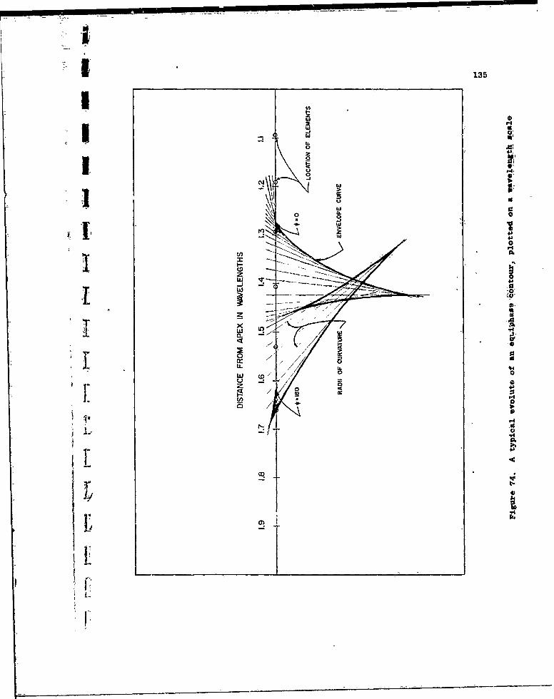
1~ 135

IIw

p4A

o>

w

4

4

IF

r 44

i

136 1

I

0.701-1

0.68 -

0.66 ,

04O.64H-PLANE,

:0.62 "p

wzP 0:60 E-PLANE

w 0.56

0.56-

0.54-

0.52-

0.50"1 I I I 1

13 13.25 I'3.50 147

LOGARITHM OF FREQUENCY

a Figure 75. Typical frequency variation of the relative distance frow

the apex to the phase center.1

.5

I]j I ii

1 137

of accuracy. An example of the measured and computed location of the phase

center is shown in Figure 76. The relative magnitude of the element base

current is also plotted so that the location of the phase center with

reference to the active region can be visualized.

i A graph-of the computed location of the phase center for models with

Z 100 and--h/a-= 177 is shown in Figure 77. x p/ is the distance to the0- p

.H-plane phase center in wavelengths, for = 00. The location'-of the

I phase center is independent of T and 7 over the rpnge of a shown. The

E-plane phase center was found to lie ahead of the H-plane phase center

by an amount which varied linearly from 0.95 x for a = 250 to x forP P

T a = 2.5 . In all cases x p < xX/2) which is the point -where the transverse

dimension is a half-wavelength. The shortening factor of Figure 33 can

be used to find the change in xp as Z0 or h/ais changed.

Since no-LP antenna exhibits a completely :.pherical equiphase surface,

the question arises as- to the utility of using point p as the phase center.

U This, of course, depends on the allowable tolerance between the zctual

- phase at some angle A', and the phase computed on the basis of an hypothetical

I! spherical wave which orignates at the phase center. Figure 78 shows an

equiphase contour S describe'd by F(C)-Or = C) where ' is the angle subtended

at the origin 0. S is an arc of radius r + d with center at po. the

- chosen phase center. S1 represents an hypothetical circular equiphase

contour of value F(o)-Bro . The error 6 F is the distance between S and S10

at the angle Y, and is given by

AF F(o) - F() d sin - sin Y= 21r + X [ sin (4, - y)] (86)

1380

-4 --

-6"

-8 i

W -10 -

M- 'A ACT.IVE .iS 12REGION

i.. -14 A.

o I"

i -18

POSITION OFH-PLANE f MEASURED

-2O0 PHASE CENTERFOR, *:0 CALCULAATEDE\

-22

-24. - 1: 700 mc POSITION OF X/2.... 800 me$ TRANSVERSE DIMENSION

-28-2I I I .. I . r I - ,I I ,I I I ,, I .

0.6 '0;7 0.8 0.9. 1.0 -1.1 1.2 1.3 1.4 1.5 1.6 1.7 1.8 1.9

X/X FROM APEX

Figure 76_. Measured And ,computed location of the phase center with referenceto the iactive region.

r'

L,.., ,.- .... 1

1 1139I

'U

4.5-zW

U) 0

z

3.0- COMPUTED POINTS:c \ Br =0.8i

-r • '-= 0.875I- \ & r =0.92

2.5 T -=0.95' "LX !X "T = 0.97

I: \ LOCATION OF HALF-

WAEENT ELEMENT

wi 1.5-z

IV)

~JJ J

2 4 6 8 10 12 -14 16 18 20 22 24 6

DEGREES

e! igure 77. Location of the phase center in wavelengths from the apex

Fl

140

kii

an

|

1 141

For the far field condition r approaches infinity and Y becomes equal to

-, reducing(80 to

6 F F(O) - F( ) d

-F2F + (1 - cos4J). (87)

If a tolerance q is given, a value 4' can be found such that

q

This defines the range of 4 over which p is a useful phase center, for

.1 the tolerance q.

Setting q = X/16 and using Equation(8, 4' was found by a trial andq

error process. Little correlation ,-zs found between 4' and the antenna

I parameters, because the phase function F was different for each antenna.

However, for all but two models in which Q is less than optimum, the value

of 4' was 900 for the E-plane pattern and greater than 900 for the H-planeq

pattern. The two exceptions were T = 0.95, O = 0.143, and T = 0.97,

= 0.175; both are high directivity models. For a greater thai, optimum,

decreased to 590 at T.= 0.875 and a = 0.222, which was the lowest valueb, q

of + recorded. Thus, in all models in the range 0.8 < T < 0.97, and

0.05 < 0 < 0.222, the error in using P as the phase center is less than

X/16 for all angles within the 3 db beamwidth.

The values of x described herein can be used as a guide in the design, P

of arrays of LPD antennas. However, due to the approximations of the theory

and the sensitivity to error of phase, it is prudent to measur'e the location

of the phase center in critical designs. An indication of the nature of the

error involved in using an incorrect value of d can be determined fro=rL

142 IEquation(WO If the error in d is Ad, then the phase error in wavelengths

will be Ad(!- cos

II 143

4. THE DESIGN OF LOG-PERIODIC DIPOLE ANTENNAS

This section first reviews the LPD parameters and their effect on

the observed antenna performance. A procedure is outlined whereby the

physical dimensions of an antenna which meets given electrical specifications

can be determined by the use of graphs and nomograms. Finally, several

I novel designs are given which exploit certain properties of log-periodic

T dipole antennas.

4.1 Review of Parameters and Effects

To varying degrees all the parameters which specify al LPD-have an

effect on the observed performance. Table 3 lists the-parameters and

I qualitatively describes how each effects the performance. The -principal

LPD parameters and their range are listed in the first two columns. At

the top of each succeeding column are the features of the antenna. The

entries denote how the performance changes with an increase in the- pertinent

parameter, while all other factors are held constant.

IThe directivity -of an LPD depends primarily on the combination of T

7 and Or selected. Directivities from7.5to 12 db over isotropic have been

measured. Since an increase in directivity implies an increased aperture,

T it is not surprising that high directivity models are characterized by

small a and large L/max . For a givca T 9, and element thickness,

T the input impedance depends- on the characteristic impedance of the feeder.

Fortunately, the directivity is essentially independent of the feeder

impedance. This makes it possible to design an antenna for a given

idirectivity and then, in most cases, the input impedance can be adjusted

to the required level. The exceptions occur on models with both low T and

low Z . Under this condition the radiating efficiency of the active region0

144

C rc)

£40 Q0 O

0 ~ N t 0 u41. on C) 0 C C 4

A'1 44 0 as os 1 .Cs.41.

0 Qs 0 4 £4o 4k

O )£0 00 C C CC

£4~~1 V -PCO -C)

0. a-=0 0Cl.4

1In 00

C '0

C 4--'C u

V. 0 04 01 0 C4. CC N~. 4, 14, -

:s C)- .4 es 0.

%) 14 0 24

0. x) 00 41~ t44.

.0y v

k, 04 2., Al 0,,p 0k0.0 a4 a) w) 'A 0 - 1 >) C) 0 0

42 ., m ) ..o C c) .0 04 4.4

4, 0, a0 40 C 0 .) at 4

..C,

0

.. 9 C

t)) 0

co mNOCC r. c -ViC)

00 0. 0.I. C4 C) C) ) 0 .4.

I145

is low, and troublesome end effects appear. Nevertheless, input impedance

levels from 50 ohms for high values of T to 200 ohms for all values of T

have been obtained. If a higher impedance level is required, the suggested

4:1 balun transformer scheme can be used.

Table 4 is a collection of the design equations. The numbers in

Jparentheses refer to the page on which the eqdations are introduced.

The most important relationship, that which relates the directivity to the

I antenna parameters, has not been put into equati-n form. For this information

reference must be made to the graph of Figure 65.

4.2 Design Procedure

First is presented a method of finding the major design parameters T

and O for a given value of directivity. Then it is shown how Z is adjusted

to obtain the required input impedance. An example which illustrates the

technique is given.

4.2.1 Choosing T and O To Obtain a Given Directivity

For most applications, one is interested in designing an antenna which

has a given -directivity and input impedance over a given frequency band.

Once these electrical characteristics are specified, one must decide the

relative importance of minimizing the number o elements or the size of

Ithe antenna. These two properties are not independent. The number of

Ielements is determined by T, as T increases the number of elements increases.

The antenna size is determined by the bc~m length (the distance between

the smallest and largest element), which depends primarily on a. As a

S d4ecreases The size increases. From the graph of Figure 65, it can be seen

JIthat a humbr of combinations of T and a lead to a given value of dir.ectivity.

(J '0

146

TABLE 4

,uxber, in parantheala refer to the page on which the equations are first Introduced

0 (1- Tcot-a r 1 4U tana a - ) 15)

Bar 1.1 + 30.7 (( rB 1.1 + 122.8 02 tan Blr 1.1 + 7.7 (1- T)2 ten a (09)

1r541 0( - r a

4Z I (1

gap%

* 120tn h/a -2.25) (53) 1

Z . 120 cosh1 (136)

a, " a r Ie)

V*0~1- j)cut a Zun.x -(, - 1, (17),B Oe B I

(6

ma F 2 - (147)

log B.

X .(127)

xp i-cota

1:I II

L .1

1 147

One of this set (T, 0) leads to minimum boom length and another leads to a

minimum number of elements.

With these facts in mind a preliminary choice of T and a can be made

from the graph of Figure 65. It is usually best to start with the optimum

value of a and then proceed to lower values. Knowing T and a, the value

j of the dependent variable a can be determined from

jj tana= (1 (89)

or from the nomograph of Figure 79.

The structure bandwidth B must be found to determine the boom length-

and the number of elements. Bs depends on the required- operating bandwidth

B and the bandwidth of the active region Bar. For the given values--of

T) and a, B r can be determined from Figure 32, or from the nomograph

of Figure 80. B is then given by~S

I B = B B. (90)S ar

Since the length of element number one is -. in the preliminary design,

the geometry of the LPD antenna provides an expression for the boom length

]U relative to the longest operating wavelength.

L (1 1-)cot a (91)

max s

where L is the boom length between the longest and shortest elements. A

nomograph of 91 is given in Figure 81. The number of elements is found

1from the equation log B

N = 1 + s (92)

a nomograph of which is given in Figure 82.

12

-. 70 2.5-

-.72 .-- ".741.4 -T4 148

.76 !,2 -3- 1.0 --. 78

.80 .801

4-

-82 .60.

-. 84 5.1

.86 .60

-. 88 7--

.20- 8-

-.90.1 - 9

.91'- 10 IC.) w

S.09 12-

S .048- 1-

D71 14-

D.5- 16-

.04 18 I-. 95

- ~20--.032

22-

-. 96 24--.96 .02- 24

264

28-

30,!-.97

01

40ih

r.98 45-

Figure 79. Nimograph, Cr -~ T) cot aI,____ _4

.2.5 70-

14.0- 7120- .73 149&0 .74-

3.0 10.0- 75-75-

8.0- 77-&5 7.0- .78

6.0- 793 4.0 .80 -

5.0- .81--4.5 4.0 .82-

.83-

• '- 5,0 S4 -

5.5 30-8

2.8-85

- 6.0 2.6- .86-1 6.5 202.2- .87-

-7.0 n2.0- .88-S-7.5 1.9- .

8 1.0- .89-8.0 0 1,-

-8.5 ( 1.79.0 I6-

-9.5 o: 1.5-

Sw WIA-

12 1,-35- .92-l1e 000~- L< -13 < 1.28 -

1.26 -93

-14 k LLI 1,24-5 0 0 L-22-

16 L20 9-

-171.8181.17

-19 .95--20 01.15-16-21 <,-

-22

24 ,96--25 --26-27 2-

-28

2930

,-34 UIO .9

-36

-38

40 1.105-

-L42

-44 _ _.98-

Figure 80. Nomograph, Ba= 1.1 + 7.7 (1 -) cot a

V

-20 2.5 --I0-8.0-6. 4A - 3-

15014.0 360.

3.5 43.0 4 1

2.82.6 2.0-

2.4 5-61.6 5

2.2 IA4

20 1.2 6-1..-"

-1.8 i.9I.801.7

1 70. 8-

iH .60- 9-

-L5 . I)10I.5Q w

<' Mco ~(D -12-1.4 .3

1 14-

H w8>3 20- 16-

1-- 16I-s-

1WJ .14- 20

.12 22

o - --- 1.3 .09 -

.08 26-

.7- 28-

.06- 30

.05-

.04-

.03 40-

.I .02 46-,

Figure 81. Nomograph, X-- 4(1 - W-)cot amax s

I-

I -.98 160- 20]

"- - " i i- 00,-_0 700- 151

90 :980-a70-760- 6

50 54540-4

356-. 96 30 3

25 ,--

20 ,A 2.6-'I- w 24--161

-M4 14" 2.2-

z 12-20 9 -o-

- L- ."w7 0

IL 9- 1.6-.92 LO M

0 Q~055--.90 ITl

4- X IA

-.85

-.80

-.75V "

-.70

log B

Figure 82. Nomograph, N = 1 . B

log

152

It is likely that the first estimate of T and U will not minimize

L or N. Repeating the process for different values of T and a will esteblish

the trend, and the minimum-designs will become readily apparent. For some

values of B minimum L cannot be attained for values of T and a within

the operating range of the graph of Figure 65. In these cases a compromise

will have to be made. If a choice of (T, 0) exists, and there is no

apparent basis for a decision it ahnld ha ra adl that +he aW inc....

and the front to back ratio decreases as a departs irom the optimum value,

according to Figures 40 and68.

Some mention should-be made of the secondary factors which effect

the directivity, Z and Z . Since the graph of Figure 65 is based onO a

Z° = 100 ohms and Za = 350, an adjustment should be made if it is

anticipated that Z° avd Z will depart from these values by more than

a factor of 2. The exact value of Z is as yet undetermined. However,

it is known that the feeder impedance is always greater than the resulting

input impedance, so if R is greater than 100 ohms the directivity contours

of Figiio 65 will read-a fraction of a decibel high. If the ratio h/a is

much different than 177 a rerection must be made. According to the curve

of Figure 71, the directivity decreases by about 0.1 db for each doubling

of h/a; for h/a > 177 the constant directivity contours of Figure 65 will

*read high. One may wish to include an additional safety factor, since a

comparison of computed and measured directivity in Table 2 shows that the

directivity compyted from Figure 65 averages 0.35 db higher than the measured

value. Th3 corrected value of directivity, for use in Figure 65, is

obtained by adding the above contributions to the required design value.

I

153

4.2.2 Designing for a Given Input Impedance

I Once the final values of T and a are found, the characteristic -impedance

of the feeder Z must be determined so as to give the required-input impedance

R . The retio h/a is determined from structural considerations, aqdideally0

3 should be the sa-me for each element. Practically, the element diameters

can be scaled in groups, and in the computation of iztput impedance the

average h/a in a group should be used. The averagechavacteristic impedane

of a dipole element Za can be found from

Za = 120 (In h/a - 2.25), (93)

or from the graph of Figure 45. Inverting Equation(71), gives the characteristic

I impedance of the feeder relative to Ro,

0: + -( ~) +1 -(94)

| ISZ 1 + -

:~R o ta [(8 . 1/ 2 94

where Z /R is the average characteristic impedatce of a dipole element with

reipect to the required input impedance Ro and a* is the mean relative

-- spacing,!/0T or/f (95)

A graph of(94)is given in Figure 46.

The major parameters of the required design have now been determined.

j It remains to find the size of the first element relative to the maximum

operating wavelength. As shown in Section 3.2.2, the longest element

can be less than for values of Z > lOG and h/a < 177. The half-e 2 0

length of the longest element is given by

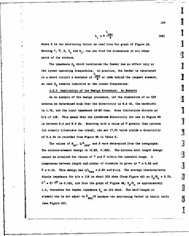
' I154

h M S max (96)1 4

where S is the shortening factor as read from the graph of Figure 33.

Knowing T, 0, N, Z and hl, one can find- tne-4mensions of all other

parts of the = antenna.

The impedance ZT which terminates the feeder has-an effect only at

the loiwest operating fliquecies. Inpractice, the feeder is terminated

in a short circuit a- distance of or -lea behind- the largest element,

so that ZT remains inductive at the lowest frequencies.

4.2.3 Application of the Design-Procedure: An Example

As an example of the design procedure, let the dimensionsof an LPDj

antenna be determined such, th1at the directivity 'in 9.5 db, the bandwidth,

is 1,75, and the input impedanci16-80-ohms. Size limitations dictate an j-h/a uf 118. This means that the corrktod'directivity for use in-Figure 65

is between 9.4 ,and-9.5 db. Starting With a value o-f greater than optimum

(to clearly illustrate the 'trend), the set (T,) which yields, a directivity

of 9.4 db is recorded from-Figure 65 in Table 5.

The values of Bar, WX~5sx and-N were determined from the nomographs.

The minimum-element design is (0.89, 0.165). The minimum boom length design

cannot be attained for vf(Lues of Tand 0 within-'the operable rangb. A

compromise between length an4 -ngmber of elements is given by T w 0.92 and

a = 0.12. This design-has L/Xmax -0.-o: and-N=12. The average characteistic

dipole impedance for h/a n 118 is about 300. ohms (from-Figure 45) so Za/ o 0 3.75.

U- - q/ VT is- 0.-126, nd from the- graph of Figure 46, Z0/R 0 is approximately

1.3, therefore the feeder, impedance Zo is 104 ohms. The half-length of

element one is set epal to.-'\/2.because th sholtening factor is nearly unity

(see Figure 33).

5 i155

TABLP 5

I Values of T, (T and a. which give 9.4 4b directivity over a 1.75:1 band

S1r L/% max

092 0.21 5.4 WLb2 2.84 1.72 13+

0.91 0.197 6.6 1.64 2.87 1.41 120.90 0.187 7.7 1.68 2.94 1.23 11+

0.89 0.165 9.5 1.66 2.91 0.99 10

0.90 0.1418 9.7 1.56 2.73 0.94 10+0.91 0.135 9.5 1.47 2.57 0.92 11-

0.92 0.120 9.5 1.40 2.45 0.89 12-0.93 0.105 9.5 1.33 2.33 0.86 13-0.9,J 0.090 9.5 1.27 2.22 0.83 14-0.95 0.070 10.2 1.21 2.12 0.7,4 15+0.96 0.051) 11.0 1.16 2.03 0.66 1+I

TABLE 6

I Antenna Dimensions in Inches

S2aDiameter of7nI h n Dn 2a1 wire used

1 1.0000 4.66 28.00 16.81 0.rf79 0.078

2 0.9200 4.29 25.76 14.57 0.073 0.0723 0.846,1 3.95 23.70 2.51 0.067 0.0724 0.7787 3.63 21.80 10.61 0.062 "J.065

5 0.7164 3.34 20.06 8.87 0.057 0.0616 0.6591 3.07 18.45 7.26 0.052 0.0507 0.606-1 2.83 16.98 5.79 0.048 0.0488 0.5578 2.60 15.62 4.43 0.044 0.0401' 9 0.5132 2.39 14.37 3.18 0.041 0.040

- 10 0.4722 2.20 13.22 2.03 0.037 0.038

1i 0.4344 2.02 12.16 0.97 0.034 0.031

12 0.3996 1.87 11.19 0 0.032 0.031

V -

vI

156 5

In compiling a table of the dimensions of the antenna, it is best

to start with a tabulation of powers of T which is accurate to at least 5four decimal places. The half lengths of the elements hn; the distance

from the apex to each element, Xn; the distance from the front of the Iantenna to each element, Dn; and the element diameters are then computed, Ias shown in Table 6. The'half length of the largest element is 4.66 ikches

because the desired low frequency cut-off is 635 mcs. 1

The feeder is spaced to give a characteristic impedance of 104 ohms

according to the formula,

Z 120 cosh - 1 b (97) 1

where b is the center to center spading and 2a is the diameter of the

feeder conductors. The above described antenna was constructed of coin

silver tubing and copper wire, using silver-solder techniques. The

resulting -model is pictured in Figure 83. The measured input impeeance

clustered around a mean resistance level R of 73 ohms, a bit lower than.

the design value. This could be brought closer to 80> ohms by increasing

the spacing between the feeders. The SWR with respect to 73 ohms is plotted

in-Figure 84. Taking an SWR of 1.3:1 to define the useful band, one finds

that this antenna operates from f to f which gives a bandwidth1.05 8,25'

of 1.82. The mesiured B-and H-plane half-power beamwidths and the

directivity ,re saown in Figure 85. The average directivity frcn f

to f8. 25 Is about 9-5 db, which just meets the requirement. A comparison

of measured and computed patterns for this antenna is shown in Figure 86.

I

III 157

III CV)

Ct

1'1 0

I 0

0

11w0

'U0

.0

0N'4

T CV)-~ 0

I TXV

V.

158

0

41

I'D-

N OR lo

cy os c cu C-SWHO Ulum u0

159

-4

UUU 0U

z .0

--

0

cl

ca-

*1Y

000.S338014K8 -lAD31 HII WV8 3.0J'V

160

"I

I / "

CO PUE - M ///E

Figure 86. Computedod and measured patterns of the-deign md

33 161

This antenna comes close to meeting tho required specifications. The

agreement between tbc measured and design value of input impedance is about

3 what can be expected. However, tne agreement between the measured ahi,

design value of directivity is somewhat better than typical; an error

of less than 0.5 db is probably as good as can be expected.

Of course, the outlined procedure is only one of many, and variations

will become apparent to those who gain experience in the design of LP

j! antennas. The concept of bandwidth of the active region and its -application

are new. Heretofore specific bandwidth designs were determined by constructing

J! an antenna which was obviously longer than necessary; the required operating

bandwidth was then obtained by a cut-and-try procedure. The graphs and

nomograms are particularly useful because they allow one to achieve many

J preliminary designs without resorting to tedious computations.

4.3 Some Novel Variations in the Log-Periodic Design

The fact that the radiating portion of an LPD at any given frequency

is confined to a relatively few elements and is independent of the location

of the front or back truncation leads to some novel departures Orom the

rtrue log-periodic forms. If it is desired to operate over two or more

separate bands, or if part of a band contains "non-int eresting" frequencies,

ithe solution is to-eliminate the elements that form the active region at

the unwanted frequencies. Tnis amounts to connecting two or more LPD

5antennas in cascade. Figure 87 shows one such-example. If the input

impedance is to remain the same over both bands, the two sections should

have the same T and a. This means that the apices of-each sec"ion will

be different. In the one model constructed according to the scheme-of

Figure 67, it was found that the presence of Section 2 lowered the low

II

162

I

~ *1 I

ii ii

4.'

-_ I2-!

I- 1-U1Ud

w!

'11

I

'I5 163

frequency cut-off of Section 1. The high frequency cut-off of Section 2

Iwas extended somewhat by the proximity of Section 1. The mid-band pa'.terns

of each section were characteristic of what would be observed with each

antenra operating by itself.

There also exists the possibility of tatilring the directivity

characteristic such that the patterns are frequency dependent in a special

Away. This would require that T and a or both be a function of position.

In this- case should be held constant to achieve a frequcnuy indepandent

input impedance. The above idea was applied- to one model in which c was

fixed at 250. The spacing between all elements was a constant, one-half

inch. 0 varied along the antenna from-0.022 to 0.088. The measured

directivity increased with frequency from 5 to 8.5 db, then decreased to 7.5 db.

IA high quality dielectric material can be used'between the elements

as well as in the feeder configuration. -The model pictured in Figure 88,

was constructed-from 0.0625'double copper-clad-Rexolite using printed

circuit :.tchlniqueg; Its parameters are T =0.92, &= 0.08, and'N= 23.

IThe equivalent h/a is 138 and Z is approximately 105 ohms. Examoles0

of the:measured patterns are shown in Figures 89 and 90. The directivity

is 8.5 db-over the band. The patterns developed scallops at the highest

frequency fi, -which was 4450 mcs. The measured cross polarization was

negligible.

The phase rotation phenomenon has been used in the design of a

frequency independent antenna whose beam is circularly polarized on the

axis. Tn this case two LPD antennas are interleaved along a common axis

with the elements of one antenna perpendicular to the other. One antenna

is also expanded with respect to the other to achieve the 90" phase shift.

V

I

C)"40'-4 I0 I'-4ci

0,0.C.C,

0

.0- IaC)o

'6'4

'C)0

£3o j4.)0

04.)

C)

C)

0 ~10

'.4

T

165

I ~f f____________ ___________

fE / LN -LN

MEASURE

Fiue8.maue atrso nLi non hc a11h, rmdobecpe-ca eoie

166

f13 f13b

E-PLANE H LN--- MEASURED

Figure go. Measured patterns of an LPD antenna which was etchedfrom double copper-clad Rexolite.

I'167 4I

Since the phase shift is independent of frequency, the pattern remainaI circularly polarized over the opbratlng band.

,1I

I-m

I:iiI

I

r

[

168

5. CONCLUSION

The object of this research wus to provide a matheatical model of Ithe log-periodic dipole antenna. The model was to be general enough to

lend insight into the operation of log-periodic antennas, and capable of

being used as a design tool. The model described herein was shown to fulfill

these objectives.

In this research the known properties of dipole antennas were used to Idetermine the self and mutual impedances in a log-periodic array of dipoles.

The properties-of the dipoles were described by an impedance matrix which

relates the voltage and current at the base of each dipole. A feeder

system, which determines the relative excitation-of each element, was

also described-by an impedance matrix. The feeder and element circuits

were joined, and the voltage and current at the base of each dipole element

were found, From these quantities the input impedance and properties of

the radiated fVeld were determined.

It was shown that three regions exist on a frequency independent

log-periodic dipole antenna: the transmission region, the active reNion,

and the -unexcited region. The transmission region was shown to be equivalent

to a section-of uniform transmission line, and the characteristic impedance

and propagation coastant of this line were determined. The active region

was shown to consist of several elements of approximately half-wavelength

dimensions on which the current amplitude is considerably greater than

that on the remaining elements. Tt, -gnitude and phase of the currents

in the activa region determines the caaracteristic pattern of the LPD, and

it was shown that the phase progression from element to element in the

I!. 1.[i

II

active region was that required to produce

the backward wave which is 1

-Icharacteristic of all LP antennas. The low input standing wave ratio

indicates that tne active region presents a good match to the transmission

I region. In the unexcited region, it was shown that in most cases a

negligible amount of power remains on the feeder beyond the active region,

and that the current In the element- that are longer than a half-wave-

,ength is very small. For these reasons the truncation at the large end of

the antenna has no effect for all frequencies within the operating band.

The bandwidth and location of the active regio.. were defined, and

these quantities were used to determine the size of an antenna which covers

a given frequency band. The relations between the observed characteristics

of the antenna, directive gain, input impedance, and location of the phase

center, and the antenna parameters were shown. A design procedure was

outlined whereby the physical dimensions of a log-periodic dipole antenna

which meets given electrical specifications can be determined. The good

Ii. agreement between measured and computed results reaffirmed once again thevalidity of certain engineering approximations that have been used since

the beginning of antenna analysis. They are, the assumption of a sin-

usoidal current distribution along straight conductors of small cross-

section, and the applicability of circuit -theory concepts to certain parts

of an antenna structure that are small compared to wavelength.

This is the first time a digital computer has been used by the Antenna

Laboratory to simulate and test a complicated, antenna model. The successful

r results of this study Indicate the possibility of utilizing the computer in

even more complex problems. It is estimated that at least seven man-days

I would be needed to build a model and perform the measurements which the

) 1.

1

I170

computer has done in a matter of minutes. On the other hand, this work 1

also illustrates one drawback in using a computer for experimental research.

That is, each model tested represents a "new" problem to the computer,

so a large mass of data must be collected to establish a trend, Perhaps Ia more sophisticated computer program could provide some data processing 1and interpolation, but in the end the utility of the results depends on the

ability of the researcher to draw conclusions from them. This is not as

easy as it may seem. Because of past training and-experience, the redearcher

has certain-prejudices that favor analysis of mathemutical equations and Inot computed data. However, once these prejudices are set aside, one will

find many new areas of research in which modern day computers can play

increasingly important roles.

UI:

.1

II

]IA

IP

I171

I BIBLIOGRAPHY

1 1. J. A. Stratton, Electromagnetic Theory, Mc Graw-Hill, New Ycrk, N. Y.,1941, p. 488.

2. A. G. -Kandojan, "Three New Antenna Types and Their Applications", Proc. IRE,

Vol. 34, pp. 70w-75w, February, 1946.

3. J. S. Chatterjee, "Radiation Field of a Conical Helix," J. Appl. Phys.,Vol. 24, p. 550, May, 1953.

I 4. V. H. Rumsey, "Frequency Independent Antennas", IRE National ConventionRecord, Pt. I, pp. 114-118, 1957. Technical Report No. 20, ContractAF33(616)-3220, Antenna Lab., University of Illinois, Urbana, Illinois,October, 1957.

5. S. A. Schelkunoff, Electromagnetic Waves, D. Va;. Nostrand Co., Inc.,New York, 1943, pp. 441-459.

6. R, L. Carrel, "The Characteristic Impedance of Two Infinite Cones ofArbitrary Cross Section", IRE Transactions, Vol. AP-6, No. 2, April, 1958,pp. 197-201. Technical Report No. 25, Contract AF33(616)-3220, AntennaLab., University of Illinois, Urbana, Illinois, August, 1957.

7. J. D. Dyson, "The Equiangular Spiral Antenna", IRE Transactions, Vol. AP-7,April, 1959, pp. 181-187. Technical Report No. 21, Contract No. AF33(616)-3220,AnteL-a Lab.-, University of Illinois, Urbana, Illinois, September, 1957.

8. J. D. Dyson, "The Unidirectional Equiangular Spiral Antenna," IRETransactions, Vol. AP-7, October 1959, pp. 329-334. Technical Report No. 33,Contract No. AF33(616)-3220, Antenna Lab., University of Illinois, Urbana,Illinois, July 1958.

9. R. H. DuHamel and D. E. Isbell, "Broadband Logarithmically PeriodicAntenna Structures," IRE National Convention Record, Pt. I, pp. 119-128,1957. Technical Report No. 19, Contract No. AF33(616)-3220, Antenna Lab.,University of Illinois, Urbana, Illinois, May, 1957.

10. D. 3. Isbell, "Non-Planar Logarithmically Periodic Antenna Structures,"Technical Report No. 30, Contract No. AF33(616)-3220, Antenna Lab.,University of Illinois, Urbana, Illinois, February, 1958.

11. D. E. Isbell, "Log Periodic Dipole Arrays," IRE Transactions, Vol. AP-8,No. 3, May, 1960, pp. 260-267, Technical Report No. 39, Contract No.AF33(616)-6079, Antenna Lab., University of Illinois, Urbana, Illinois,June, 1959.

12. H. E. King, "Mutual Impedance of Unequal Length Antennas in Achelon,"'IRE Transactions, Vol. AP-5, No. 3, July, 1957, pp. 306-313.

13. 0. Zinke, "Fundamentals of Voltage and Current Distributions along Antennas,"V Arch. Rlektrotech., Vol. 35, pp. 67-84, 1941.

172 114. R. L. Bell, C. T. Elfving, R. 8. Franks, "Near Fieli Measurements on

a Logarithmically Periodic Antenna," Technical Memorandum r.DL-M231,Contra:ct No. DA-36-039-SC-78281, Electronic Defense Laboratories, IMountain View, California, December, 1959.

15. S. C. Jordan, Electromagnetic Waves and Radiating Systems, Prentice-Hall, 1'Inc., New York, 1950, p. 464.

16. 2. Siegel and J. Labus, "Apparent Resistance of Antennas," Hochf. andElck., Vol. 43, 1934, p. 166.

17. P. E. Mayes, G. A. Deschamps, W. T. Patton, "Backward Wave Radiationfrom Periodic Structures and Application to the Design of FrequencyIndependent Antennas," Proceedings of IRE, Vol. 49, -No. 5, May, 1961.

18. R. L. Carrel, "The Pe r gn-of ±og-Pericdic Dipole Antennas," 1961 IRE

International Convention Record, pt. I, March, 1061.

19. Smith Electronics Co., Brecksville, Ohio, Private Communications.

20. P. E Mayes and R. L. Carrel, "Logarithmically Periodic Resonant-

V Arrays," Technical Report No. 47, Contract No. AF33(616)-6079, AntennaLab., University of Illinois, Urbana, Illinois, Jaly, 1960.

21. J. D. Kraus, Antennas, Mc Graw-Hill, New York, N. Y., 1950, p. 25.

22. R. H. Dufamel and F. R. -Ore, "Log-Periodic Feeds for Lens and Reflectors,"

IRE National Convention Record, pt. I, 1959, p. 128.

23. R. H. DuHamel and D. G. Berry, "Logarithmically Periodic AntennaArrays,"I IRE WESCON Convention Record, pt. I, August, 1958.

24. Z. Jahnke and F. Emde, Tables of Functions, Dover Publications,New York, 1945.

25. Tables of Sine, Cosine, and Exponential Integrals, Federal Works Agency,

Work Projects Administration for the City of New York, sponsored by the BNational Bureau of Standards, 1940.

26, H. S. Wall, The -Analytic Theory of Continued Fractions, D. Van Nostrand

Co., Inc., New York, 1948.

27. G. Kron, Tensor Analysis of Networks, J. Wiley & Sons, Inc., New York,f N. Y., 1939.

28. J. D. 1-json) "Measuring the Capacitance Per Unit Length of BiconicalStructures of Arbitrary Cross Section," Technical Report No. 29, Contract INo. AF33(616)-3220, Antenna Lab., University of Illinois, Urbana,

Illinois, -January, 1958.

29. G. A. Deschamps, "Impedance Properties of 'nmplementary MultiterminalPlanar Structures," Technical Report No. 43, Contract No. AF33(616)-6079,Antenna Lab., University of Illinoia, Urbana, Illinois, November, 1959.

I!

173

30. R. H. DuHamel "Logarithmically Periodic Circuits," Research DivisionTechnical Mem'randum, Collins Radio Company, Cedar Rapids, Iowa, November,1960.

1 31. R. H. DuHamel and F. R. Ore, "Logarithmically Periodic Antenna Designs",1958 IRE National Convention Record, pt. I, p. 139.

1 32. R. E. Franks and C. T. Elfving, "Reflector-Type Periodic BroadbandAntennas," 1958 IRE WESCON Convention Record, p. 266.

33. R. H. DuHamel and.D. G. Berry, "A New Concept in High Frequency AntennaDesign ," 1959 IRE National Convention Record, pt. I, p. 42.

34. J. R. Tomlinson and M. N. Fullilove, "Very Broadband Feed for ParaboloidalReflectors," 1959 IRE National Convention Reccrd, -pt. I, p. 147.

35. J. K. Shimizee, E. M. J. Jones, and R. C. Honey, "A Sinuous Flush-Mounted Frequency Independent Antenna," Technical Report No. 3, ContractNo. AF19(604)-3502, Stanford Reseaich Institute, Oct~Ober, 1959.

36. D. E. Isbell, "A Log-Periodic Reflector Feed," Proc. IRE, Vol. 47,p. 1152, June, 1959.

T 37. P. S. Mayes and R. L Carrel, "Logarithmically Periodic Resonant-VArrays," Technical Report No. 47, Contract AF33(616)-6079, AntennaLab.,* University of Illinois, Urbana, Illinois, July, 1960.

38. R. L. Carrel, "Analys's of the Log-Periodic Dipole Antenna," Abstractsof the 10th Annual Syposium on Air Force Antenna Research and Develop-ment, University of Illinois, October, 1960.

39. D. G. Berry and F. R. Ore, "Log-Periodic Monopole Array," CullinsResearch Report No. CRR-220, Collins Radio Company, Cedar Rapids,Iowa, October, 1960; 1961 IRE International Convention Record, pt. I,March, 1961.

- 40. J. )V. Carr, "Some Variations in Log-Porioedic Antenna Structures,"Trans. IRE., Vol. AP-A, pp. 229-230, March, 1961.

41. H. Jasik, Antenna Engineerine Handbook Mc Graw-Hill, New York, N. Y.,1961, Chapter 18.

p'

174

APPENDIX A 174

COMPUTATIONAL CONSIDERATIONS

This section describes several pirts of the computer program for the

solution of the equations of Section 2. The expansions used to evaluate -

Lhe jine- and cosine-integral functions are given in detail, and the /

mg.hod used to solve the system of linear equations is outlined. ,

Since the accuracy of the over-all program depends on the accuracy

of the veveral parts, care was taken to avoid progrpmming blunders which Ilead to accumulated round-off errors. Each section of the program was

checked by-special test routines and compared with calculations performed

on a desk calculator before being incorporated into the whole. In general,

priority was placed on accuracy rather than computational spoed, and

standard ILLIAC library routines were used wherever possible,

A.1 The Cosine- and Sine-Integral FUnctions

The cosine-integral and sine-integral functions are definqdas24

Ci(x) - f cosu du (98)

and

Si(x)=J sin- -du (99)

Two distinct methods were used to compute E(x) = Ci(x) + j Si(x), For

0 < x < 6 a series expansion was used. For x > 6-a continued fraction

expansion was used., The crossover point x =--6 was determined by the

computer time required to achieve 8 or 9 accurate significant digits, using

either method. A plot of computer time vs. x is shown in Figure 91. The

crossover 'pint x i 6 was chosen from this plot. The series representations

-,

I

K'~~ - z , z -- -

II175

12

II'

1 80I I

0

- 7IDo 6--

w

-w

3 /1

2

0 I . . I I , I I I I I0 I 2 3 4 5 6 7 8 9 10

ARGUMENT x

Figure 91. Computation time vs. argument x for the series and-continuedfraction expansion of K(x) = Ci(x) + j St(x)

I-

T

F

176

used were

25

00 (l) n2n

Ci(x) = C + 1n(x) + E (2n), 2 n (100)

n=l

where C = 0.57721 is Euler's constant, and

Go n2n + ISi(x) = nl _(2n + 1) j (2nX+71) (101)

Boch the above series are uniformly convergent for all finite values of x.

The convergence of these seriesis slow, and the number of terms required-

for a given accuracy increases with x. Fifteen terms were required for

eight place accuracy with x equal to-6. However the terms of the-series

are monotonically decreasing and alternating in sign, so the error involved

In using n terms is numerically less than the n + 1st term. This fact

allows one to compute until a given accuracy is attained, Und this-

advantage outweighs the fact that the convergence is slow. The two

series of Equations 100 and- 101 were computed together as

K(x) = C + -n(x)- nl n n (102)

To -find the continued fraction expansion for-K(x) observe that

K(x) = Ci(x) + JSi(x) = Ei(jx) + J, (103)

where 0

-Ei(-z) = du (104)U

As a function of the complex variable z. Ei(-z) has a logarithmic branch

point at z = 0, therefore the argumtent z =z1 eje is restricted such that

-v < 6 'I. A continued fraction exp.4nsion exists for (104), 26L _________

II

177

eZf O u 1= -- -- - (105)ez du 1 1 2 2 3 (rs

f z

By means of an equivalence transformation (105) can be rewritten

Iez ez- du =I 1 I 1 1 1(106)

e u z + + +1 + 4+ + -+ 10.1 z2 3

This is a continued fraction of Stieltjes. The general form of the Stieltjes

continued fraction is

1 1 1 (107)

k + k + k3z + k' + ks 4- k + ...1 2 3 4 5 6

The continued fraction (107) is uniformly convergent in the cut z-plane due

to the fundamental convergence theorem-of Stieltjes, which states that if

the k are positive constants and the series E k diverges the continuedP p

fraction is uniformly converE-nt over every finite closed domain of z whose

distance from the--negative half of the real axis is positive, and its

value is an analytic function of z for all z not on the negative half of

the real axis. Therefore K(x) may be computed from (106). By means of

-another equivalence transformation,

K(x) =J + (108)jx F~jx)

whereF(Jx) I I1/Jx 1/Jx 2/Jx 2/Jx 3/ix

1 - 1 - 1 - 1 - 1 ... (109)

The pth approximate of F, AP/Bp, is given by the fundamental recurrence

formulas:

I

178

Ap + b P + A p + ap + 1 A .1

(110)

B +i bp +i Bp + ap + 1 B p iwith

A-, 31, B1 =0, A= b 0 B° =1, (ii)

and -(p + 0)/2

ap -(p +p = 1,3,5, "'', I

a - p = 2,46, "', (112)

bp =x.

1.

The fundamental recurrence formulas allow one to compute the successive

approximates of F rather than start with a given p and ationalize F p

In the ILLIAC program for -the continued :fraction expansion of K(x), it

was found that nine place accuracy for Ci(x) or Si(x), whichever was larger,

was achieved when

A A

for x > 1.5. The number of iterations required ranged from 73 for x = 1.5

to 15 for x = 9.

The subroutine for X(x) was programmed to test x to determine the type

of expansion to use and then to compute K(x) to nine sigificant digits. It

is worthy of note that continued fraction expansions exist for many trans-

cendental functions, some of which are given by Wall? and that in certain

cases the continued fraction is more rapidly convergent than the corresponding

series expansion.

1 179

5 A.2 Matrix Operations

The program which computes T (U + YFZA) was straightforward. . The prime

3L difficulty in this case is the systematic addressing of the storage locatlons

of the matrix elements.

The solution of

1 1= T -A (114)

employs the upper triangularization and back-substitution method. The

I steps in this method are as follows. Fist the augnented matrix Ta is

I s set up, using T and Y.

t11 t12 t3 ---- tlN 1l

21 2223 2N 2

a

L Nl N2 N3 NN N

Here the t 1s are the elements of T and the ii's are the elements of .

Ya is a matrix which represents the equation

I - 1= 0 * (116)_ A

- By the elementary determinate operations, Ta can--be upper triangularized

yielding

1 t --- t12 13 1,N+1

t23 ---- t2N+

0 0- t-- ~~~N 0 --- I N+1

180

iA N iA N-1 A N-2 ... can be successively determined by a series of back-

substitutions,

iAN t NN+l

(118)

/ /iAN_1 = N-i, N i - N-1 N iAN

Several test matrices were employed to check the accuracy of this

part of the program. It was found -that nine significant digit accuracy

was preserved in solving equations- in four unknowns. Nine significant

digits is the maximum accuracy that can be obtained-using the ILLIAC in

the floating-point mode. It was expected that the accuracy decreased

as the number of equations increased. However, a sample calculation of

an eight element antenna using the entire LPD, analysis program, agreed

in the first five significant digits with the computations performed on

a desk calculator (which, incidently, ,took three weeks to perform).

1 181

5 APPENDIX B

5 MEASUREMENT CONSIDERATIONS

This section discusses several types of measurements which were per-

3 formed in the experimental phasu of this research. The procedure used in

the measurement of the near field amplitude and phase will be considered

I in detail, whereas the input impedance, radiation pattern, and phase center

. measurements will be given only summary remarks. Except for the near field

phase measurements standard techniques were used, and a majority of problems

SI that arose were concerned with the application of these techniques to the

particular antenna structures under investigation.

I In any measurement involving log-periodic or log-spiral structures,

one is faced with the problem of obtaining a great amount of data over a

wtde range of frequencies, if the frequency independence of the antenna

is to be confirmed. The large bandwidth (4:1 or greater) over which the

measurements must. be performed places certain requirements on the

experimental set-up and on the construction of the model. The experimental

T set-up must be changed several times throughout the course of a measurement

because of the relatively narrow bandwidth of some testing equipment. This

f means that certain pieces of equipment are operated under slightly differing

conditions, hence the set-up should proide for easy calibration and tuning.

IOf equal importance is the actual fabrication of the model antenna.

Construction tolerance should be figured on the basis of the shortest wave-

length of operation. Thus, to some extent, the size of the antenna is

determined uy the accuracy which can be maintained in the model shop. The

transverse dimensions of the feeder configuration of an LPD must remain small

compared to the length of the zhortest element. Nevertheless, the minimum

T182

diameter of the feeder members is limited by the size of the internal

feed coax. This again places a limit on the size of the antenna and the

range of useful testing frequencies.

The above requirements led to the choice of the 100 mcs to 400 mcs Irange for the models used for impedance and near field measurements. A

picture of one of the impedance models is shown in Figure 92. The feeder Idiameter was 0.420 inches, just large enough to accommodate the teflon dielectric 3RG-115 A/U coaxial cable which was choseh for its low loss and excellent

uniformity. The pattern models were built for the 500 mcs to 2000 mcs range,

the low frequency limit being dictatpd by the antenna pattern range facilities.

B.1 Near Field Measurements

The near field mcasurements consisted of determining the amplitude and

phase of the voltage between the feeder conductors and the current into each

dipole element. The voltage between the feeder conductors was found by 4measuring the signal received by a small probe antenna as pictured in Figure

93. The coax which energizes the antenna model runs trough one of the hollow

feeders. The other -feedrir member is equipped with a milled slot which -jguides the probe assembly throughout the length of the antenna. The probe

is connected to a length of RG 58/U coaxial cable which is contained in a -

thin walled tube. The end of the tube opposite the probe assembly Is fitted

with a pointer which moves along the length of a rule, permitting accurate

and repeatable positioning of the probe. The input impedance of the antenna

was found to change 1.4% as the position of the probe was changed from the

front of the antenna to the back. This is due to a small change in the I

feeder impedance owing to the presence of the milled slot. The variation

II-

18I' _ _ _ _ _ _

r

Fiue9.ApcueoIn fteatensue o erfedmaueet

184 ~

M 4)0 $4 -

w0 ow 0

4 ii

0 4)

z U )

z w

J 0 A

w 0LI-

< 4)

CL~f 0; 41

w z0 #--

a - 0

-LJ '1

o 4-0

DIzI

z'

185

I of the measured data was found to be independent of the length of the probe,

which was varied from one eight to one quarter inch.

The measurement of the dipole element current was accomplishad by the

loop probe shown in Figure 94. The loop was designed to measure the

magnetic field encircling the dipole, and was located as close to the base

I of the dipole as possible. Many difficulties were encountered in the selection

of the proper loop size, spacing, and location. Shielding waj necessary,

as indicated by initial results with an anshielded loop. However, a

I completely shielded loop could not be constructed small and accurately,

because there was no space to extend the pick-up coax through the guide

1 assembly. The partially shielded loop in Figure 94 was selected as a

comprom .se. The figure also shows the delectr~c disk which encloses the

loop. This device was used to accurately position the loop at a constant

Td~stance from the dipole and in a pla-e containing the dipole element andthe loop. The diameter of the loop and the dielectric was chosen such that

a minimum amount of transverse motion was required in going from an element

F. connected to one feeder to an element connected to the other. The configuration

shown in Figure 94 was found to yield repeatable results aithough effects

of undesired field components were never entirely eliminated. The largest

extraneous component was thought to be due to the proximity of the current

on the neighboring dipoles. It was estimated that this component was

down at least 15 db from the desired component. The agreement between

measured and computed results of the element current is therefore not

as good as that of the feeder voltage.

B.1.I Amplitude Measurements

T-A block diagram of the ciicuit used for the amplitude measurements is

186

U -

WI14

w 0 m

z uA

w w 0 a 3

0 c

~~tO a - 0[

0 =) 2

)0 0 0J

I cI

II

187

3 shown in Figure 95. The filtered output of the square wave modulated power

oscillator is delivered to the antenna through a double stub tuner, which

was adjusted for maximum signal to the probe. The square law detected out-

put of the tuned probe is displayed on a SWR amplifier, peak tuned to the

modulation frequency of 1000 cps. In performing the measurement, the

I probe was moved back and forth until the location of maximum signal was

found. This point was taken as the 0 db reference. A readirg wai tuken

every centimeter throughout the length of the anterna. A power output

from the oscJllator on the order7 of 5everal watts was required for a

dynamic range of 40 db above noise.

I B.1.2 Phase Measurements

The phase measuring circuit is diagrammed in Figure 96. The principal

features are the hybr1 junction and the balanced input adapter. The

Imeasurement theory is as follows: A CW reference signal, whose phase can

be adjusted by means of the slotted se, tion and linp stretcher, is injected

into the series arm (4) of the hybrid junction. The modulated test signal

r" feeds the shunt arm (3). The RF phasor sum of these signals is impressed

across the load connected to output (1) and the phasor difference appears

at output (2). The balanced input adapter takes the audio difference of

these detected signals from the hybrid junction arid also provides the bias

voltage for the bolometers. As shown in Figure 97, a sharp null is observed

at the output of the balanced adapter when the reference signal is 900 out

of phase with the test signal. Figure 97 compares the phasor relations and

1 the nulls obtained cf the balanced detection method and the single detection

method. In the latter method only the difference channel would be used; the

null is obtained when the reference and test signals are in phase, provided

188

F1114 Y0z c

z

.4o

.J w

ww

0 w 0a 0

0: 0

U. L0J 0

I. 1 IOw

0: w

LL 4)

w 0I--E .00100

00'4

wI

I w 189

3~~C 0. 1 .jf

0 .4 x

IL>1 0

000.

8,51

0.0 w S

mw o 0

Ii U-n 0 VI-w w

0 01

CD-

LuzU4 L -------- ------ -------

-j Ilk

-Col.

190

ii-E ET - ER E EIE'ERp

IETI - ER IETTER ETR ET

I ER

1ETI R IETI ER

JERI IER.I

II

ET-ER ET ET'I-ER

ET-ER ET ER "ER

J IE- - 5 0 = 0 o -T E .I = .5 ,/ = 9 0 0

SINGLE DETECTION BALANCED DETECTION I2.0\ = 2.o0 -2.CJERI 1 JERI

1.5 IE -IEr

- w 1.5

ww'4 .0 . a:--

12 w.5-4 .. 5

0So o i-180 0 180 0 90 180

SDEGREES 1 DEGREES

Figure 97. Phasor relations and the nulls obtairted for values of .1I,. I/IE for two methods of measuring relative .hase.ET R I-)aeET is the test signal, ER is the reference signsl.

J I

1 191

5 both signals have equal amplitude. Since the amplitude of the test signal

varies, this method wou! require a precision variable attenuator calibrated

3 for amplitude and phase. The advantage of the balanced detection system is

that a well defined null is obtained even when the test and reference signals

are of unequal amplitude. However a 1800 ambiguity exists in the balanced

j detection method. This can be resolved by carefully following the incremental

phase shift as the probe is moved away from the reference position.

1 For phase measurements the probe signal, rather than the oscillator

is modulated. This results in a sharper null than would otherwise be obtained.

.1 Even though the unmodulated refereice signal, which may be larger than the

1 test signal. is present at the detectors, the result is only a DC componentIof current to the transformer. The only error from the reference signal

is due to leak-through in the hybrid junction. This is negligible; in

dommei.cially available instrument hybrids the decoupling is on the order

of 50 db.

The experimental set-up for the near field phase measurements is shown

in Figure 98. All the equipment was mounted on a bench whilh could be rolled

up to a second story window in the Antenna Laboratory, in order for the

model under test to look into an uncluttered environment. The most predominaut

feature In the picture is the take-up reel for the cable which is zonnected

to the probe. In the phase measurements it is important that t~e flexing

of the (able be controlled and held to a minimum; the take-up reel serves

I this purpose.

The following procedure was carried out to balance the hybrid circuit

-- after each change of frequency. Refer to Figure 96. The connection at

IX terminal (4) is broken and replaced with a matched load. The bias to

~~~~192

44,4

"'.4

'4

IV?

I(

1 193

each bolumetor was adjusted to 8.75 ma. One bolomeer was then disconnected

and thi balancing potentiometer was adjusted for maximum output. The

I tuning stubs throughout the circuit were then tuned for maximum output.

The other bolometer was reconnected and the first was disconr.ected. The

balancing potentiometer was again adjusted for maximum output, and only

the stubs associated with the operative bolometer were tuned, the others

were left as previously adjusted. With both bolometers connected, the

1. baloncing potentiometer was adjusted to null the skgnal. This step had

the effect of balancing out any leak-through component of the test signal;

it also equalized any residual unbalance which might have existed between

the two bolometers. The slotted line was reconnected, completing the tune-up

procedure.

The probe was positioned at a chosen point and the phase of the reference

p" signal was changed to obtain a null. This was repeated every centimeter

along the feeder of the antenna. By recording the phase change introduced

by the slotted line, the relative phase of the test signal was determined.

B.2 Impedance Measurements

f. The input impedance of the LPD models was determined by the SWR and

null shift method. The set-up incorporated a PRD standing wave indicator

or alternatively a HP slotted line, and a tuned amplifier using a bolometar

* detector.

The short circuit reference plane for the impedance measurements was

taken at the front of the antunna, as shown in Figure 99. This choice of

a reference plane lumps the gap or terminal impedance in with the antenna

impedance. For this reason, extra care was taken in the construction of

I the feed region. After several trials it was found that the feed region

Lf

194KREFERENCE PLANE

METAL ELBOWFOR SYMMETRY

,FEED COAX i

I~k

CONDUCTORS

CONDUCTOR [Pigure 99. Details of the symmetrical feed point, showing the

reference plane for impedance measurements

i

1

195

configuration shcwn in Figure 99 was best from the standpoint of introducing

a minimum unbalanced current component and a minimum gap reactance. Ideally,

the reference measurement should be made at every frequenvy, ju:z- before or

after the co. responding load measurement. This was not done because of

the large number of test frequencies involved and because of the uncertainty

in reconstructing an identical feed configuration each time. Instead, the

electrical length of the coax from the reference plane to a reference on

the measuring device was determined for all the f'equencies within the band,

prior to taking the load measurements. Several lengths of cable were testea;

the one which yielded the most uniform results was used.

B.3 Far Field Measurements

The radiation patterns of the LPD modes were recorded by the commercially

equirqed University of Illinois Antenna Lab-3ratory patcern range facilities.

The tower and ap LPD model are pictured in Figure 100. Using a bolometar

as the square law detector, the system was found to have a linear dynamic

range of greater than 20 db. Since the LPD models tested had an operating

bandwidth of 3:1 or greater, interference from other sources operating

within this band sometimes presented a problem. Except for the signal

from an S-band radar that was 250 yards away, the interference problem was

i±iminated by filtering and tuning techniques.

The phase center measurement wcrc cccp shcd . .. n. the . ... ,,

detector shown in Figure 96, except that the model under test assumed the

role of the probe antenna. The test model was mounted on a tower in such

a way that the axis of rotation could be moved toward or away from the

transmitting antenna. The relative phise of the received signal was plotted

as a function of the azimuth angle over the range + 40 degrees from the dead

F _ _ _ _ _ _ _ _ _ _ _ _ _ _ _ __ _ _ _ _ _ _ _ _ _ _ _ _ _ _ _ _ _ _

196

rI

ILL

I

1 197

3 ahead position. The center of rotation of the model was varied from one

plot to the next until a position was found such that the phase was most

U nearly constant over the range of the azimuth angle. The bornsight and

positioning accuracy was such that the location of the phase center could

be determined within an error of + 0.125 inch, which was about 0.01 > at

the testing frcqucncies.

1I

i1-

I"

7

* ANTENNA LABORATORY*TECHNICAL REPORTS AND MEMORANDA ISSUED

Contract AF33 (616)-310

"Synthesis of Aperture Antennas," Technical Rcoort No. I C.T. A. Johnk,jOctober, 1954.*"A Synthesis Method for Broad-band Antenna Iz'pedance Matching Networks,"

Technical Report No. 2, Nicholas Yaru, 1 February 1955.*

"The Asymmetrically Excited Spherical Antenna , Technical Report No. 3PRobert C. Hansen, 30 April 1955,41

"Analysis of an Airborne Homing System, Technical Riport No. 4 Paul E.Mayes, 1 June 1955 (CONFIDENTIAL).

I"Coupling of An~tenna Elcnients to a Circular Surface Waveguide , TechnicalReport No. 0u 1%. E. King and R,. 11, Dullamel, 30 June 1955.*

I"Axially Excited Surface Wave Antennas, Technical Report No. 7 D. E. Royal,10 October 1955.*

"Homing Ant:~inas for the F-86F Aircraft (450..2500mc)," T,,chnic-al R ep o rt No-_1P. E. Mayes, H. F. Hyneman, and R. C. Becker, 20 February 1957, (CONFIDENTIAL).

"Ground Screen Pattern Range, I'Technical Memorandum No._ 1 Roger R. Trapp,II 10 July 1955.*

FContract AF33(616)-3220Effective Permeability of Spheroiual Shells, Technical Report No. 9, E. J.Sotand R. H. Dullamel, 16 April 1956.

An.Analytical Study of Spaced Loop ADF Antenna Systems , Technical Report

No 1 -D. -G. Berry Rnd J. B. Kreer, 10 May 1956.

"A Technique for Controlling the Radiation from Dielectric Rod Waveguides,"

T~cffiigiLk-Report No. 11 J. W. Duncan and R. H. DuHamel. 15 Yuly 1956.*

"Directional Characteristies of a U-Shaped Slot Antenna, Technical ReportNo..12 -Richard C. Becker, 30 September 1956.**

!'txW~ceof Ferrite Loop Antennas," Technical Repoit No. 13. V. H. RumseyadW.L. !±4ek-s 15 Oc-tober 1956.jJ oey--pcd-Trnves Slots in Rectangular Waveguide," Technical Report

xo ~ kcor-F yea 20 December 1956.

I N,>4,I

--

I

"Distributed Coupling to Surface Wave Anteqas," Technical Report Nu. 15,

Ralph Richard Hodges, Jr., 5 January 1957. 1"The Characteristic Impedance of the Fin Antenna of Infinite Length , TechnicalReport No, 16, Robert L. Carrel, 15 January 1957.*

"On the Estimation of Ferrite Loop Antenna Impedance, Technical Report No. 17,Walter L. Weeks, 10 April 1957.*

"A Note Concerning a Mechanical Scanning System for a Flush Mounted Line Source IAntenna," Technical Report No. 18, Walter L. Weeks, 20 April 1957.

"Broadband Logarithmically Periodic Antenna Structures," Technical Report No. 19R. H. DuHamel and D. E. Isbell" 1 May 1957.

"Frequency Independent Antennas," Technical Report.No V. H. Rumsey 25 October 1957.

"The Equiangular Spiral Antenna," Technical Report No. 21, J. D. Dyson 15

September 1957.

"Experimental Investigation of the Conical Spiral Aattenna," Technical ReportNo. 22.R. L. Carrel, 25 May 1957.**

"Coupling between a Parallel Plate Waveguide anda Surface Weveguide," Technical

Report-No. 23 E. J. Scott, 10 August 1957.

"Launching Efficiency of Wires and Slots for a Dielectric Rod Waveguide,"Technical Report No. 24, J. W. Duncan and R. H. DuHamel, August 1957. 3"The Characteristic Impedance of an Infinite Biconica2 Antenna of ArbitraryCross SAction ," Technical Report No. 25, Robert L. Carrel, August 1957. 1"Cavity-Backed Slot Antennas," Technical Report Noq 26 R. J. Tector, 30October 1957.

"Coupled Waveguide Excitation of Traveling Wave Slot Antennas," TechnicalReportNo. 27 W. L. Weeks, 1 December 1957.

"Phase Velocities in Rectangular Waveguide Partially Filled with Dielectric,"Technical Report No. 28, W. L. Weeks, 20 ')ecember 1957.

"Measuring the Capacitance per Unit Length of Biconical Structures of ArbitraryCross Section," Technical Report No. 29, J D. Dyson, 10 January 1958.

"Non-Planar Logarithmically Periodic Antenna Structure," Technical Report No. 30 JD. W. Isbell, 20 February 1958.

"Electromagnetic Fields in Rectangular Slots," Technical Report No. 31 N. J.Kuhn and P. E. Mast, 10 March 1958. ["The Efficiency of Excitation of a Surface Wave on a DielectriV Cylinder ,

Technical Report No. 32, J. W. Duncan, 25 May 1958.

I

jI!U

"A Unidirectional Equiangular Spiral Antenna, Technical Report No. 33,J. D. Dyson, 10 July 1958.

"Dielectric Coated Spheroidal Radiators, Technical Report No. 34 W. L.

m3 Weeks, 12 September 1958.

"A Theoretical atudy of the Equiangular Spiral Antenna," Technical ReportN 3 P . E. Mast, 12 September 1958.

I Contract AF33(616)-6079

"Use of Coupled Waveguides in a Traveling Wave Scanning Antenna," Technical

Report No. 36, R. H. MacPhle, 30 April 1959,

' "On the Solution of a Class of Wiener-Hopf Integral 2quaticas in Finite and

Infinite Ranges," Technical Report No. 37, Raj Mittra, 15 May 1959.

"Prolh'e Spheroidal Wave Functions for Electromagnetic Theory," TechnicalReport No. 3.Fj W. L, Weeks, 5 June 1959.

"Log Periodic Dipole Arrays," Technical Report No, 39 D. E. Isbell, 1 June 1959.

"A Study of the Coma-Corrected Zoned Mirror by Diffraction Theory," TechnicalReport No. 40, S. Dasgupta and Y. T. Lo, 17 July 1959.

"The Radiation Pattern of a Dipole on a Finit. 91electrJc Sheet," Technical

-Report No. 41 K. G. Balmain, 1 August 1959.

"The Finite Range Wiener-Hopf Integral Equation and a Boundary Value Problem

in a Wavegulde" Technical Report No. 42, Raj Mittra, 1 October 1959.

"Impedance Properties- of Complementary Multiterminal Planar Structures,"Technical Report No. 43. G. A. Deschamps 11 November 1959.

I "On the Synthesis of Strip Sources," Technical Report No. 44 Raj Mittra4 December 1959.

S " Numerical Analysis of the Eigenvaluc Problem of Waves in Cylindrical Waveguides,"

Technical Report No. 45, C. H Tang and Y. T. Lo, 11 March 1960.

"New Circularly Polarized Frequency Independent Antennas with Conical Dliam or

Omnidirectional Patterns," Technical Report No. 46, J D. Dyson and P. E. Maves,

20 Jure 1960.

"Logarithmically Periodic Resonant-V Arrays," Technical Report No. 47, P. E. Mayesand R. L. Carrel, 15 July 1960

"A Study of Chromatic Aberration of a Coma-Corrected Zoned Mirror," TechnicalReport No. 48 Y. T. Lo.

1

_________ _____. . . ..____ ____ __________ __________

"Evaluation of Cross-Correlation Methods in the Utilization of Antenna Systems,"Technical Report No. 49, R. H. MacPhie, 25 January 1961.

"Synthesis of Antenna Product Patterns Obtained from a Single Array," Technical

Report No. 50, R. H. MacPhie.

* Copies available for a three-week loan pcriod.

** Copies no longer available.

V.V]

]

! .1

II

I

AF 33(616)-6079

DISTRIBUTION LIST

One copy each unless otherwise indicated

Armed Services Technical Information A r Force Ballistic Missile DivisionAgency Attn: Technical Library, Air Force

Attn: TIP-DR Unit Post OfficeArlington Hall Statior Los Angeles, CaliforniaArlington 12, Virgini (10 copies)

DirectorAeronautical Systems Division B4l1istics Research LaboratoryAttn, (ASRNRE-4) Aitt.: Ballistics Measurement Lab.

I Wright-Patterson Air Force Base Aberdeen Proving Ground MarylandOhio (3 copies)

National Aeronautics & Space Adm.Aeronautical Systems Division Attn: LibrarianAttn: ASDSED, Mr. Mulligaa Langley Field VirginiaWright-Patterson Air Force BassOhio Rome Air Development Center

Atty: RCLTMAeronautical Systems Division Griffiss Air Force BaseAttn: ASAD - Library New YorkWright-Patterson Air Force BaseOhio Research &- Development Command

Hq USAF (ADRD-RE)Aeronautical Systems Division Washington 25, D. C.Attn: AFCIN-4BlAWright-Patterson Air Force Base Office of-Chief'Signal OfficerOhio Engineering & Technical Division

Attn: -SIGNET-5Air Force Cambridge Research Washington-25, D. C.

LaboratoryAttn: CRRD CommanderLaurence G. Hanscom Field U. S. Army White Santl Signal AgencyBedford, Massachusetts Attn: SIGWS-FC-02

White Sands, New Mexico

Attn: PGTRI, Technical Library 801 Air DivilonEglin Air Force Base Attn: DCTIDFlorida Lockbouine Air Force Base

Oh A eiCommanderAir Force Missile Test Center DirectorPatrick Air Force Base Surveillance Department

Florida Evans AreaAttn: Technical Document Center

Commander Belmar, New JerseyAir Force Missile Deveionnent CenterAttn; Technical Library CommanderHolloman Air Force Base U. S. Naval Air Test CenterNew Mexico Attn: WST-54, Antenna Sction

Patuxent River, Maryland

Material Laboratory, Code 932 Amphenol-Borg Electronic CorporationNew York Naval Shinyard Attn: Librarian (Antenna Section)Brooklyn I, New York 2801 S. 25th AvenueBroadview, Illinois ICommanding

Officer

Diamond Ordnance Fuse Laboratories Bell Aircraft CorporationAttn: 240 Attn: Technical LibraryWashington 25, D. C. (Antenna Section)

Buffalo 5. New York

DirectorU. S. Navy Electronics Laboratory Bendix Radio Division ofAttn: Library Bendix Aviation CorporationSan Diego 52, California Attn: Technical Library

(For Dept 462-4)

National Bureau of Standards Baltimore 4, MarylandDepartment of CommerceAttn: Dr. A. G.. McNish Boeing Airplane CompanyWashington 25Y D. C. Aero Sps'e Division

Attn: Technical Library

Adams-Russell Company M/F Antenna & Radomes Unit

200 Sixth Street Seattle, WashingtonAttn: Library (Antenna Section)CambridgeJ Massachusetts Boeing Airplane Company

Attn: Technical Library

Aero Geo Astro M/F Antenna Systems Staff UnitAttn: Security Officer Wichita, Kans.-

1200 Duke StreetAlexandria, Virginia Chance Vought Aircraft Inc.

THRU: BU AER -RepresentativeNASA Goddard Space Flight Center Attn: Technical -Library -Attn: Antenna Soction, Code 523 M/F Antenna Section 1Greenbelt, Maryland P. 0. Box 5907

Dallas 22, Texas

Airborne Instruments Labs., Inc.Attn: Librarian (Antenna Section) Collins Radio Company

Walt Whitman Road Attn: Technical Library (Antenna

Melville, L. Io. N.Y. Section)Cedar Rapids, Iowa

American Electronic Labs

Box 552 (Antenna Section) Convair

Lansdale, Pennsylvania Ft, Worth Division JAttn: Technical Library (Antennh

American Systems Inc. Section)Attn: Technical Library Grants Lane

" ......a ... .. .~in) Fort Worth, Texas

3412:Century Blvd.Inglewood, California Convair

Attn: Technical Library (Antenna

Andrew Alfred Consulting Engineers Section)

Attn: Librarian (Antenna Section) P. 0. Box 1950

299 Atlantic Ave. San Diego 12, California iBoston 10, Massachusetts

J -I

I{

i Dalmo Victor Company Goodyear Aircraft CorporationAttn: Tcchnical Library (Antenna Attn: Technical Library

Section) M/F Dept 4741515 Industrial Way 1210 Massilon RoadBelmont, California Akron 15, Ohio

Dorne & Margolin, Inc. Granger AssociatesAttn: Technical Library (Antenna Attn: Technical Library

Section) Antenna Section30 Sylvester Street 974 Commercial StreetWestbury, L, I., N. Y. Palo AltIo, California

* Dyatronics Inc. Grumman Aircraft Engineering Corp.Attn: Technical Library (Antenna Attn: Technical Library

Section) (N/F Avionics Engineering)Orlando, Florida Bethpage, New York

I Electronic Communications, Inc. The Hallicrzfters CompanyResearch Division Attn: ,rechnical Library (AntennaAttn: Tecnnical Library Sectfon)1830 York Road 4401 W. Fjfth AvenueTimonium, Maryland Chicago 24, Illinois

Fairchild Engine & Airplane Corporation Hoffman Laboratories Inc.Fairchild Aircraft & Missiles Division Attn. Technical Library (AntennaAttn: Technical Library (Antenna Section)

Section) Los Angeles 7, CaliforniaHagerstown 10, Maryland

John Hopkins UniversityGeorgia :nstitute of Technology Applied Physics LaboratoryEngineering Experimznc Station 8621 Georgia AvenueAttn: Technical Library Silver Springs, Maryland

M/F Electronics DivisionAtlanta 13, Georgia Hughes Aircraft Corporation

Attn: TechnicaJ Library (AntennaGeneral Electric Company Section)fl Electronics Laboratory Florence & Teal StreetAttn: Technical Library Culver City, CaliforniaElectrotnics ParkSyracuse, New York University of Illinois

" Attn: Technical Library (Dept ofGeneral Electronic Labs., Inc. Electrical Engineering)Attn! Technical Library (Antenna Urbana, Illinois

Scctlon18 Ames Street ITT LaboratoriesCambridge 42, Massachusetts Attn: Technical Library (Antenna

Section)General Precision Lab., Division of 500 Washington Avenue

General Precision Inc. Nutley 10, New JerseyAttn: Technical Library (Antenna

Section)63 Bedford RoadPleasantville, New York

L

Lr

ILincoln Laooretories University of Michigan

Massachusetts Institute of Technology Radiation LaboratoryAttn: Document Room Willow Run

P. 0. Box 73 201 Catherine StreetItexington 73. Massachusetts Ann Arbor, Michigan

Litton Industries Mitre CorporationAttn: Technicil Library (Antenna Attn: Technical Library (M/F Elec-

Section) tronic Warfare Dept. D-21)4900 Calvert Road Middlesex TurnpikeCollege Park, Maryland Bedford, Massachusetts ILockheed Missile & Space Division New Mexico State UniversityAttn: Technical Library (M/F Dept- Attn: Technical Library (M/F

58-40., Plant 1, Bldg. 130) Antenna Dept)Sunnyvale, California University Parkj New Mexico

The Martin Company North Ame-ican Aviation Inc. IAttn: Technical Library (Antenna Attn: Technical Library (M/F

Section) Engineering Dept.)P. 0. Box 179 4300 E. Fifth Avenue IIDenver 1, Colorado Columbus 16, Ohio

The Martin Company North American Aviation Inc.

Attn: Technical Library (Antenna Attn: Technical LibrarySection) (M/F Dept 56)

Baltimore 3, Maryland International Airport

Loc Angeles, CaliforniaThe Martin CompanyAttn: Technical Library (M/F Northrop Aircraft, Inc.

Microwave Laboratory) NORAIR DivisionBox 5837 Attn: Technical Library IIOrlando, Florida (M/F Dept 2135)

Hawthorne, California

W. L. Maxson Corporation

Attn: Technical Library (Antenna Ohio State University Research

Section) Foundation

460 West 34th Street Attn: Technical LibraryNew York 1. New York (M/F Antenna Laboratory)

1314 Kinnear RoadMcDonnell Aircraft Corporation Columbus 12, Ohio [IAttn: Technical Library (Antenna

Section) Philco CorporationBox 516 Government & Industrial DivisionSt. Louis 66, Missouri Attn: Technical Library I

(M/F Antenna Sectfmn)Melpar, Inc. 4700 Wissachickon AvenueAttn: Technical Library (Antenna Philadelphia 44, Pennsylvania 0

Section)

3000 Arlington Blvd.Falls Church, Virginia

L i

II Radio Corporation of America H. R. B. Singor Corporation

RCA Laboratories Division Attn: Librarian (Antenna Lab)Attn: Technical Lib-ary State College Pennsylvania

(M/F Antenna Section)Princeton. New Jersey Sperry Microwave Electronics Company

Attn: Librarian (Antenna L4b)

* Radiation Inc. P. 0. Box 1828Attn: Te~hnical Library (M/F) Clearwater. Florida

Antenna SectionDrawer 37 Sperry Gyroscope CompanyMelbourne, Florida Attn; Librarian (Antenna Lab)

Great Neck, L. I., New YorkRaiioplane CompanyAttn: Librarian (M/F Aerospace Lab) Stanford Electronic Laboratory8000 Woodly Avenue Attn: Librarian (Antenna Lab)Van Nuy3, California Stanford California

Ramo-Wonldridge Corporation Stanford Research InstituteAttn: Librarian (Antenna Lab) Attn: Librarian (Antenna Lab)Conoga Park, California Menlo Park, Californlu

Rand Corporation Sylvania Electronic SystemAttn: Librarian (Antenna Lab) Attn: Librarian (M/F Antenna &

1700 Main Street Microwave Lab)Santa Monica, California 100 First Strest

Waltham 54, MassachusettsRantec CorporationAttn: Librarian (Antenna Lab) Sylvania Electronic System23999 Ventura Blvd. Attn: Librarian (Antenna Lab)Calabasas, California P, 0. Box 1881" Mountain View, California

Raytheon Electronics Corporation

Attn: Librarian (Antenna Lab) Technical Research Group" 089 Washington Street Attn: Librarian (Antenna Section)

. Newton, Ma3sachusetts 2 Aerial WaySyosset, New York

Republic Aviation CorporetionApplied Research & Development Ling Temco Aircraft Corporation

Division Temco Aircraft Division

Attn: Librarian (Antenna Lab) Attn: Librarian (Antenna Lab)L Farmingdale, New York Garland, Texas

Sanders Associates Texas Instruments Inc.Aitn: Librarian (Antenna Lab) Attn: Librarian (Antenna Lab)95 Canal Street 6000 Lemmon Ave.Nishua, New Hampshire Dallas 9, Texas

, Southwest Research Instituta A. S. Thomas Inc.Attn: Librarian (Antenna Lab) Attn: Librarian (Antenna L.b)8500 Culebra Road 355 Providence HighwaySan Antunio, Texas Westwood, Massachusetts

Ii

IWestinghouse Electric Corporation Dr. Harry Letaw, Jr. IAir Arms Division Raytheon CompanyAttn: Liurarlan (Artenna Lab) Surface Radar and NavigationP. 0. Box 746 Operations

State Road West IWheeler Laboratories Wayland, Massachusetts

Attn: Librarian (Antenna Lab)Box 561 Dr. Frank Fu FangSmithtown) New York IBM Research Laboratory

Poughkeepsie, New York

Electrical Engineering ResearchLaboratory Mr. Dwight Isbell

Uriversity of Texas 1422 lth WestBox 8026, Univ. Station Seattle 99, WashingtonAustin, Texas

Dr. A. K. Chatterjee

University of Michigan Research Vice Pri'cipalInstitute Brla Engineering College

Electronic Defense Group Pilani, RajasthanAttn: Dr. J. A. M. Lyons IndiaAnn Arbor. Michigan INew Mexico State UniversityHead Antenna DepartmentPhysical Sci. i Laboratory IUniversity Park, New Mexico

Bell Telephone Laboratories Inc. fWhippany Laboratory

Whippany, New Jersey -,

Ati: Technical Reports Librarian IRoom 2A-165

Robert C. Hansen

Aerospace CorporationBox 95085Los Angeles 45, California -1

Dr. D. E. Royal

Ramo-Wooldridge, a division ofThompson Ramo Wooldridge Inc.

8433 Fallbrook AvenueCanoga Park, California

Dr. S. Dasgupta _Government Engineering CollegeJabalpur, M.P.

India

Dr. Richard C. Becker

10829 BerkshireWestchester, Illinois

.I

R _ ° L

Documents

UNCL ASSI11!11FIED - apps.dtic.mil · 4.1 Review of Parameters and Effects 143 4.2 Design Procedure 145 4.2.1 Choosing T and U To Obtain a Given Directivity 145 4.2.2 Designing for