Embed Size (px)
Citation preview
UNCLASSIFIED
AD 400926
)FENSE DOCUMENTATION CENTERFOR
SSCIENTIFIC AND TECHNICAL INFORMATION
CAMERON STATION, ALEXANDRIA, VIRGINIA
UNCLASSIFIED
NOTICE: When government or other drawings, speci-
fications or other data are used for any purpose
other than in connection with a definitely related
government procurement operation, the U. S.
Government thereby incurs no responsibility, nor any
obligation vhatsoever; and the fact that the Govern-
ment may have formulated, furnished, or in any way
supplied the said drawings, specifications, or other
data is not to be regarded by implication or other-
wise as in any manner licensing the holder or any
other person or corporation, or conveying any rights
or permission to manufacture, use or sell any
patented invention that my in any way be related
thereto.
'.t
1I T A

NOT RELEASABLE
TO OTS
LECTURES IN APPLIED MATHEMATICSProceedings of the Summer Seminar, Boulder, Colorado, 1960
VOLUME I
LECTURES IN STATISTICAL MECHANICSBy G. E. Uhlenbeck and G. W. Ford with E. W. Montroll
VOLUME II
MATHEMATICAL PROBLEMS OF RELATIVISTIC PHYSICSBy 1. E. Segal with G. W. Mackey
VOLUME III
PERTURBATION OF SPECTRA IN HILBERT SPACEBy K. 0. Friedrichs
VOLUME IV
QUANTUM MECHANICSBy V. Bargmann
A STIA A
APR121 : 1
€0TISIA
0
0Q
LECTURES IN APPLIED MATHEMATICSProceedings of the Summer Seminar, Boulder, Colorado, 1960
VOLUME Iby
G. Ep UHLENBECK and G. W. FORDwith
E. W. MONTROLL
0
Mark Kac, EditorThe Rockefeller Institute
S SQ
o0
B0
iU
I, li. Lectures inStatistical Mechanics; '
by
S-.E. UHLENBECKTHE ROCKEFELLER INSTITUTE
G. W. FORDPROFESSOR OF PHYSICS, UNIVERSITY OF MICHIGAN /
WITH AN APPENDIX ON
Quantum Statistics of Interacting Particlesby
E. W. MONTROLLRESEARCH CENTER, INTERNATIONAL BUSINESS MACHINES CORPORATION
$ -1 %3
, "- 1, '* "/ '$ r* ,7 "< / , :,
AMERICAN MATHEMATICAL SOCIETY
PROVIDENCE, RHODE ISLAND
(:v ?/ ..
Copyright C 1963 by the American Mathematical Society
The Summer Seminar was conducted, and the proceedingsprepared in part, by the American Mathematical Societyunder the following contracts and grants:
Grant NSF-G12432 fron; .he National Science Founda-tion.
Contract No. AT(30-I)-2482 with the United StatesAtomic Energy Commission.
Contract Nonr-308 1(00) with the Office of Naval Research.Contract DA-19-020-ORD-5086 with 'the Office of
Ordnance Research.All rights reserved except those granted to the United StatesGovernment, otherwise, this book, or parts thereof, may notbe reproduced in any form without permission of thepublishers.
Library of Congress Catalog Card Number 62-21480
Printed in the United States of America
Foreword
This is the first of a series of four volumes which are to contain theProceedings of the Summer Seminar on Applied Mathematics,arranged by the American Mathematical Society and held at theUniversity of Colorado for the period July 24 through August 19,1960. The Seminar was under the sponsorship of the NationalScience Foundation, Office of Naval Research, Atomic EnergyCommission, and the Office of Ordnance Research.
For many years there was an increasing barrier between mathematicsand modern physics. The separation of these two fields was regret-table from the point of view of each-physical theories were largelyisolated from the newer advances in mathematics, and mathematicsitself lacked contact with one of the most stimulating intellectualdevelopments of our times. During recent years, however, mathe-maticians and physicists have displayed alacrity fpr mutual exchange.This Seminar was designed to enlarge the much-needed contact whichhas begun to develop.
The purpose of the Seminar was primarily instructional, withemphasis on basic courses in classical quantum theory, quantumtheory of fields and elementary particles, and statistical physics,supplemented by lectures specially planned to complement them.The publication of these volumes is intended to extend the sameinformation presented at the Seminar to a much wider public thanwas privileged to actually attend, while at the same time serving as apermanent reference for those who did attend.
Following are members of a committee who organized the programof the Seminar:
Kurt 0. Friedrichs, ChairmanMark KacMenahem M. SchifferGeorge E. UhlenbeckEugene P. Wigner
Local arrangements, including the social and recreational program,V
vi FOREWORD
were organized by a committee from the University of Colorado, asfollows:
Charles A. HutchinsonRobert W. Ellingwood
The enduring vitality and enthusiasm of the chairmen, and thecooperation of other members of the university staff, made the stayof the participants extremely pleasant; and the four agencies whichsupplied financial support, as acknowledged on the copyright page,together with the Admissions Committee, consisting of BernardFriedman, Wilfred Kaplan, and Kurt 0. Friedrichs, Chairman, alsocontributed immeasurably to the successful execution of the plans forthe Seminar.
The Seminar opened with an address given by Professor Mark Kac,Department of Mathematics, Cornell University, on the subject "AMathematician's Look at Physics: What Sets us Apart and WhatMay Bring us Together." Afternoons were purposely kept free togive participants a chance to engage in informal seminars anddiscussions among themselves and with the distinguished speakers onthe program.
Editorial Committee
V. BARGMANNG. UHLENBECKM. KAC, CHAIRMAN
Contents
PREFACE ixL. THE EXPLANATION OF THE LAWS OF THERMODYNAMICS 1
I1. THEORY OF THE NON-IDEAL GAS 32II. REMARKS ON THE CONDENSATION PROBLEM 61IV. THE BOLTZMANN EQUATION 77V. THE PROPAGATION OF SOUND 89
VI. THE CHAPMAN-ENSKOG DEVELOPMENT 102VII. THE KINETIC THEORY OF DENSE GASES 118
APPENDIX: QUANTUM STATISTICS OF INTERACTING
PARTICLES
By E. W. MONTROLL 143INDEX 179
vii
Preface
These lectures were given by one of us (G. E. U.) as a part of thesummer symposium in theoretical physics, which was organized by theAmerican Mathematical Society at the University of Colorado in thesummer of 1960. The lectures are printed here almost in the sameform as they were presented, which explains the rather colloquialstyle and the perhaps excessive use of the first personal pronoun.This last feature does not mean that the content of the lectures is dueonly to the first author. All lectures were thoroughly discussed andprepared by both of us, and most of the developments for which someoriginality may be claimed are the result of the collaboration of thetwo authors during many years.
The purpose of the summer symposium was to acquaint a group ofmathematicians with some of the basic problems in present-daytheoretical physics, hoping that this would stimulate a more intensecollaboration. In our opinion such a collaboration would be especiallyvaluable in statistical mechanics, since here many of the unsolvedproblems can be formulated precisely and are of a technical mathe-matical nature. Furthermore, because of the lack of exact knowledgeof the intermolecular forces, one is usually more interested in theexplanation of the qualitative features of the macroscopic phenomenathan in the precise quantitative prediction of the macroscopic quantities.This qualitative aspect of the theory should appeal to the mathe-matician while for the physicist it is often a real difficulty. Since thefacts are so well known the latter is often tempted to be satisfied withmore or less uncontrolled approximations based on intuitive argu-ments. These are often very valuable, but usually they do not provide,so to say, a foothold for a rigorous mathematical treatment. In ouropinion such a treatment is especially needed in statistical mechanics,and to provide it is the real challenge of the subject.
We have therefore stressed as much as possible the logical structureof the theory, and we have always tried to indicate the mathematicalgaps which remain in the argument. In addition we have tried tostart from the beginning and to avoid as much as possible the phrase:it can be shown. Proofs are often put in the notes at the end of eachchapter together with references to the literature. We hope that as
ix
X PREFACE
a result the book can be used as a short but self-contained introductionto the subject, although we realize that it will have to be used withtact, since the textbook-like chapters alternate with chapters describingwork still in progress.
To achieve, even only approximately, these rather conflicting goals,it soon became clear to us that we had to limit the field considerably.Not only have we restricted ourselves to the simplest possible physicalsystems (namely mono-atomic gases) but even for these systems wecould only discuss a few characteristic problems. The most severelimitation we had to impose was the restriction to the classical theory.This is fortunately somewhat mitigated by the two lectures Dr. E.Montroll gave, which are reproduced in the Appendix. Here anaccount is given of some of the recent developments in quantumstatistics to which Dr. Montroll himself has made such importantcontributions.
In one respect we did not want to limit ourselves. It is oftencustomary either to consider only the statistical problems for theequilibrium state (sometimes called statistical thermodynamics), or toconcentrate on the explanation of the irreversible and transportphenomena (sometimes called kinetic theory). It seems to us thatsuch a limitation gives a distorted view of the subject, and that oneshould try to give a unified treatment both of equilibrium and non-equilibrium statistical mechInics. We have therefore devoted sixlectures (reproduced in the first three chapters) to equilibrium prob-lcms and six lectures (reproduced in Chapters 4-7) to non-equilibriumproblems, and we have attempted to point out at least the conceptionalconnections between the two fields.
Finally there remains the pleasant duty to thank in the first placeProfessor Mark Kac for all the help and advice he has given us. Ifthese lectures would inspire one other mathematician of the calibre ofProfessor Kac to work on the problems of statistical mechanics thesymposium would have more than justified itself! The reader wouldalso be well advised to read in parallel with these lectures the thirdchapter in the book Probabilit, and Related Topics in Physical Sciences,by Professor Kac, since the outlook is in many respects the same asours. Then we want to thank Professor T. H. Berlin for manydiscussions and for his permission to use a few parts of a manuscripton which he and one of us (G. E. U.) have been working for quitesome time.
G. E. UHLENBECK
G. W. FORD
CHAPTER I
The Explanation of the Lawsof Thermodynamics
I. Introduction. In this chapter I will try to present an outline of thefoundations of statistical mechanics, and I must apologize for the factthat it will not be a clear, axiomatic presentation. This is not becauseI am, as some physicists are, impatient with general discussions offundamentals. On the contrary, I believe that further progress isintimately connected with a further clarification of the foundations.However, at present there is no generally accepted opinion of what thebasic assumptions of the theory are, and as a result I can only presentmy own point of view, which is, I believe, a kind of paraphrase of thefundamental ideas of Boltzmann and Gibbs. And since these ideaswere mainly developed in the attempt of explaining the laws of thermo-dynamics from the molecular theory of matter, I will follow also inthis respect in the footsteps of the two founders of statisticalmechanics.'*
First, let me remind you of the general problem of statistical physics.Given the structure and the laws of interaction of the molecules,what are the macroscopic properties of the matter composed of thesemolecules? To start one has therefore to say something about themolecular model and about the basic microscopic laws. For sim-plicity I will almost always assume:
(a) The motion of the molecules is governed by classical mechanics.It is true that the quantum mechanics adds new features to the prob-lem; it may even be that the act of measurement introduces a "true"irreversibility into the theory as some authors claim. But most of theessential questions arise already in the classical theory, and since it ismore familiar to you, I will restrict myself to this theory.
(b) The molecules are mass points interacting through centralforces, which have the additivity property and which are of the van
* Numbers refer to Notes at end of Chapter.
2 THE EXPLANATION OF THE LAWS OF THERMODYNAMICS
der Waals or molecular type. This means that the given Hamiltonianof the system of N particles is of the form:
(N H= 2m 1(I) H= [A + U(r,)J + #I 0r 1 - r1 )
IIl J<j
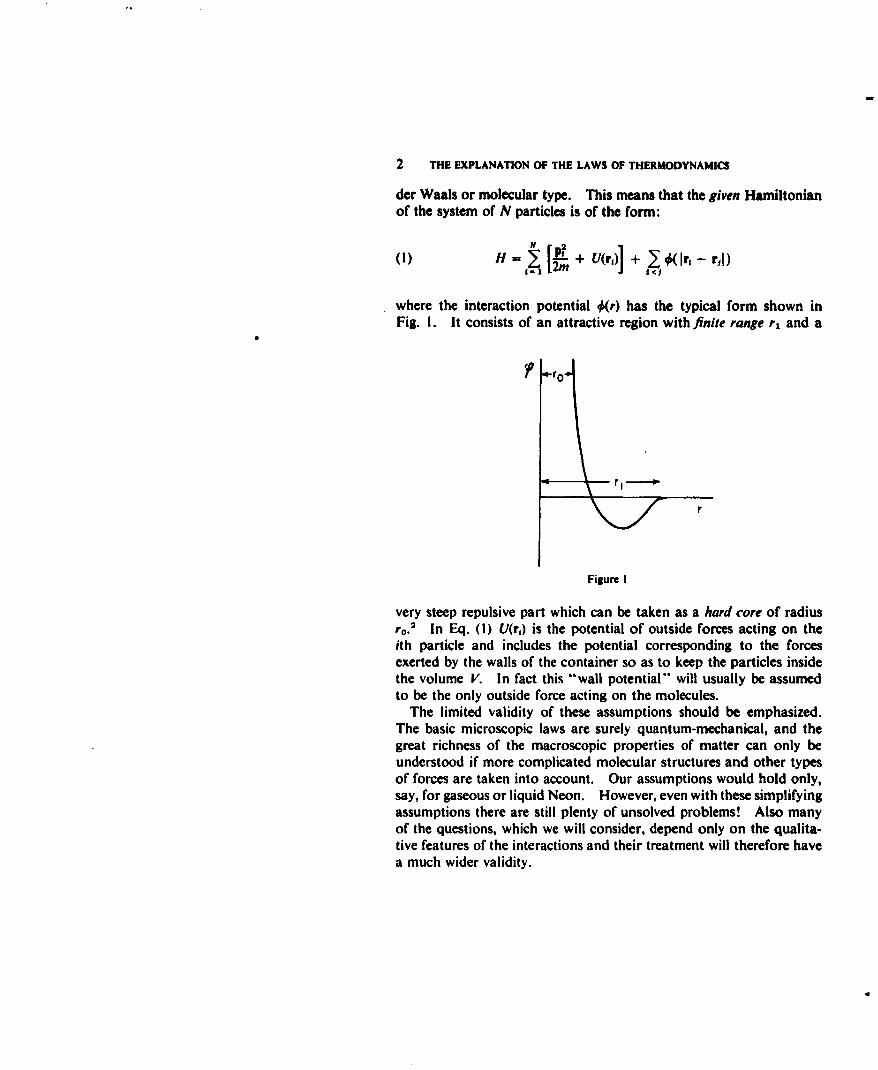
where the interaction potential 0(r) has the typical form shown inFig. I. It consists of an attractive region with finite range r, and a
ro
Figure I
very steep repulsive part which can be taken as a hard core of radiusr o.2 In Eq. (1) U(r1) is the potential of outside forces acting on theith particle and includes the potential corresponding to the forcesexerted by the walls of the container so as to keep the particles insidethe volume V. In fact this "wall potential" will usually be assumedto be the only outside force acting on the molecules.
The limited validity of these assumptions should be emphasized.The basic microscopic laws are surely quantum-mechanical, and thegreat richness of the macroscopic properties of matter can only beunderstood if more complicated molecular structures and other typesof forces are taken into account. Our assumptions would hold only,say, for gaseous or liquid Neon. However, even with these simplifyingassumptions there are still plenty of unsolved problems! Also manyof the questions, which we will consider, depend only on the qualita-tive features of the interactions and their treatment will therefore havea much wider validity.
THE LIOUVILLE THEOREM 3
2.1 "Lioullle dteorem. We represent the state of a mechanicalsystem of n degrees of freedom by a point in the 2n-dimensional phasespace or r-space. In our case n = 3N, N = number of particles,and the coordinates of a point in P-space are r1*.. rN, Pi "'PN. Inthe course of time this P-point will move according to the Hamiltonequations of motion:
OH OH(2) 0 - ' i 1,2, ...,n.
Since these equations are of first order in the time it is clear that thepath of the representative point in P-space will be determined by theinitial point. To visualize the motion for all possible initial points,imagine that one has a very large number of copies of the system.Each copy sends a point in V-space, and if the number is large enough,one may consider the collection of points as a fluid streaming inP-space and possessing in any point a certain number densityp(q1...q,,p..p.,t). The streamlines of the fluid motion areidentical with the particle paths as determined by (2). With Gibbswe call this the ensemblefluid or just an ensembk of mechanical systems.One should note that the total number of copies never plays a roleand is only introduced as an aid to visualize all the possible motionsof the P-point. The ensemble fluid is a true continuum, and insteadof the streaming of the fluid it may be better to speak of a continuousmapping of the P-space in itself. Soon also the density p will becomethe probability density that the system is in a region dq1... dp. ofP-space, and we shall then denote it by D(q ... p., t) and assume thenormalization condition:
f... fdql ... dp. D= l.
In addition if the N particles are identical one should require that Dbe a symmetric function of the phases (r,, p,) of the separate particles.
A theorem which plays a central role is the theorem of Liouville,3
which states that the ensemble fluid moves as if it were an incompressibkfluid.
To prove this, note that the "velocity" V (components q..,il... fulfills the condition:
( Qv+ V.)(3) divV a 1" 2,") •~ . XS, • = 0
4 THE EXPLANATION OF THE LAWS OF THERMODYNAMICS
by virtue of the Hamilton equations. Since one always has thecontinuity equation:
Op + div (pV) = 0
or:Dp
(4) D- + pdiv V = 0
with
D a(5) + V.grad
+ i1 + p
it follows from (3) that:
(6) Dt
which means that p does not change if one moves with the fluid, orthe fluid is incompressible.
If one stays at a fixed point in F-space then p changes according to:
e- + V-grad p = 0
or:(7) Lp (OH ep 1H 1_p) H'(-7)= • ap, eP) q = {H, p}
where (H, p} is the Poisson bracket of Hand p. This is the "Eulerian"way of expressing the incompressibility of the fluid. In the "Lagran-gian " way of describing the motion of the fluid, the position (qr* • 'p.)of a fluid element is given as a function of the initial position (qjo • . pR0)and of the time. The condition for the incompressibility of the flowis now that the Jacobian:
(8) Paq o ... p.)ij~qjo ""PRO)
which expresses the fact that if one follows a whole volume of pointsduring the flow, this volume always stays the same, although of course
THE APPROACH TO EQUILIBRIUM; THE IDEAS OF BOLTZMANN 5
its shape will vary. Or in other words: the transformation of theV-space into itself induced by the flow preserves volumes. It is easyto see that the characterizations (7) and (8) are completely equivalent.
Two simple consequences of the Liouville theorem are worthnoting:
(a) For any function F(p) of the density, the integral:
f . .. f F(,) dq, I ... dp.
taken over the whole F-space is independent of the time.(b) Any density distribution p will be stationary, i.e. will not depend
explicitly upon the time, if and only if p is constant along each stream-line. In particular any distribution p(H), which is a function of theHamiltonian H, will be stationary, although such distributions are byno means the only stationary ones.
3. The approach to equilibrium; the ideas of Boltznman. How can one"explain" the irreversible behaviour of macroscopic systems from thestrictly reversible mechanical model? This question, which I call theproblem of Boltzmann, has dominated the whole initial developmentof statistical mechanics and it is still being discussed. In its simplestform, one must "explain" in which sense an isolated (that is a con-servative) mechanical system consisting of a very large number ofmolecules approaches thermal equilibrium, in which all "macro-scopic" variables have reached steady values. This is sometimescalled the zeroth law of thermodynanies and it expresses the mosttypical irreversible behaviour of macroscopic systems familiar fromcommon observation.
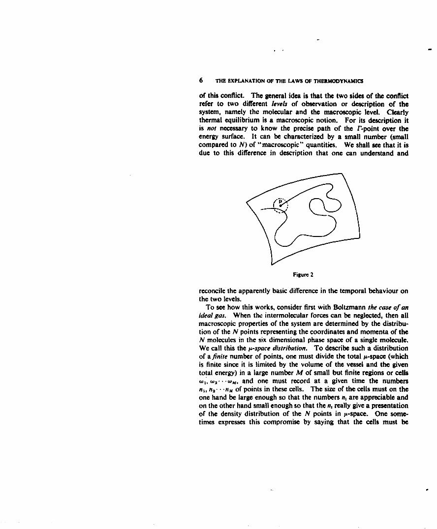
The conflict with mechanics is most drastically shown if one recallsthe famous Poincare recurrence theorem. For a conservative system,the motion of the r-point will stay on the energy surface H(q1 ... )= E. Furthermore the motion is bounded (in the momenta by thetotal energy E and the finite attractive potential energy; in the co-ordinates by the volume in which the molecules are enclosed). Forsuch a mechanical system starting from a point P on the energy surface,the theorem says that for an), region around P, there is a time T inwhich the phase point of the system will return to the region (seeFig. 2). Or in other words, the motion is quasi periodic, and there isapparently no trace of an approach to equilibrium. An outline of theproof of the Poincar6 theorem is given in the notes.4
Let me now try to sketch the classical Boltzmann-Gibbs resolution
6 THE EXPLANATION OF THE LAWS OF THERMODYNAMICS
of this conflict. The general idea is that the two sides of the conflictrefer to two different levels of observation or description of thesystem, namely the molecular and the macroscopic level. Clearlythermal equilibrium is a macroscopic notion. For its description itis not necessary to know the precise path of the /-point over theenergy surface. It can be characterized by a small number (smallcompared to N) of "macroscopic" quantities. We shall see that it isdue to this difference in description that one can understand and
Figure 2
reconcile the apparently basic difference in the temporal behaviour onthe two levels.
To see how this works, consider first with Boltzmann the case of anideal gas. When the intermolecular forces can be neglected, then allmacroscopic properties of the system are determined by the distribu-tion of the N points representing the coordinates and momenta of theN molecules in the six dimensional phase space of a single molecule.We call this the IA-space distribution. To describe such a distributionof a finite number of points, one must divide the total jL-space (whichis finite since it is limited by the volume of the vessel and the giventotal energy) in a large number M of small but finite regions or cellsW1 , W2 ... WJ, and one must record at a given time the numbersn1, n2 " • .nM of points in these cells. The size of the cells must on theone hand be large enough so that the numbers n, are appreciable andon the other hand small enough so that the nj really give a presentationof the density distribution of the N points in ju-space. One some-times expresses this compromise by saying that the cells must be
THE APPROACH TO EQUILIBRIUM; THE IDEAS OF BOLTZMANN 7
"physically infinitesimal". It is a compromise which always must bemade in the description of an empirical distribution of a finite numberof discrete entities.
Clearly the distribution n1 , n2 ' •. over the cells w,, w2 " . . in J,-spacedescribes the state of the gas much less precisely than the descriptionby one point in F-space. Each point in F-space corresponds to adefinite distribution in 1s-space, but the reverse is not true. In factit is easy to prove that a given distribution in s-space corresponds to awhole region (6N-dimensional) in F-space which has the volume:
(9) W = N! - w ;&"2... 'A(.nj! n2 ! ... nM! 1 2 "
PROOF. Clearly the distribution n, will not change if we move themolecules around in their cells. Moving, say, one of the moleculesin the first cell around, leaving all other molecules fixed, will move thecorresponding r-point over a six-dimensional volume W1. Since inF-space the states of the different molecules are represented byorthogonal six-dimensional sub-spaces, the motion of all N moleculesin their cells will move the /-point over a "block" in F-space of thevolume:
(10) U " "U.
In addition the distribution n, will not change if we permute twomolecules in different cells and the motion of the molecules in theircells after the permutation will again produce a block of size (10) inF-space, which will have no common region with the previous block.Since there are:
(I N!(11) Nnj! n2! ... nu!
ways of dividing the N molecules in groups ni, n2 ", the total volumein F-space will be given by the product of (10) and (II).
The set of numbers n, is restricted by two subsidiary conditions:
In,= N,(12)
1 E
8 THE EXPLANATION OF THE LAWS OF THERMODYNAMICS
which express the conservation of total number and of total energy.Here ej denotes the energy of a particle in the cell w,. That one canassign this energy independently of the occupation numbers of thecells is clearly due to the assumption of the ideality of the gas. Notealso that in (12) the value of E is not precisely determined, because theF, will vary slightly when the points move in their cells. The E in(12) is therefore not strictly the same as the given energy which deter-mines the energy surface H(q, p) = E in V-space on which the /-pointmoves. In fact the energy condition (12) determines two neigh-bouring energy surfaces around the given energy surface. Theregion in between we will call the energy shell; its thickness clearlydepends again on the finiteness of the cells wd in IA-space.
NEquilibriumS~state
S• Non-equilibrium
states
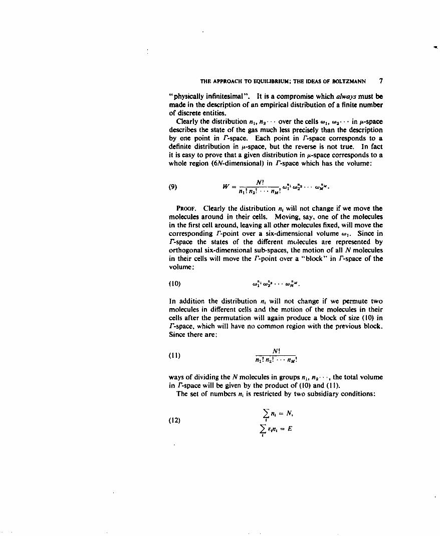
Figure 3
The volumes W(n1 , n ... ) of the different distributions n, over thecells w, in IA-space (as given by (9)) will cut out of the energy shellcylindrical regions of different size. Now one can prove thetheorem :'
If N is very large then the so-called Maxwell-Boltzmann (M.B.)distribution:
(13) f, = Awo,e-,
corresponds to a volume W which cuts out the overwhelmingly largestportion of the energy shell. In (13) the A and P are constants whichmust be determined from the subsidiary conditions (12). Schemati-cally the division of the energy surface in /-space by the various
THE GENERALIZATION BY GIBBS. THE ERGODIC THEOREMS 9
volumes W(ni, n,...) is shown in Fig. 3. Boltzmann now identifiesthe M.B. distribution in 1,-space with the thermal equilibrium state ofthe gas, and all other 1s-space distributions with the macroscopicnon-equilibrium states of the gas.
If we now assume, that in the motion of the V-point over the energysurface there is no preference for any portion of the surface and thatin the course of time every accessible part of the surface will bereached, then it is very plausible that the time t(A) during which theV-point is inside a region A is mainly determined by the magnitude ofthe area of A. Clearly one can then conclude:
I. If the gas is not in the thermal equilibrium state (- M.B.distribution), then it almost always will go into this state.
2. Once the gas is in the equilibrium state it will almost alwaysstay there, although fluctuations away from equilibrium will andmust occur because of the quasi-periodic character of the motion ofthe V-point.
This is the Boltzmann picture. It clearly reconciles the reversibilityof the mechanical motion as expressed by the Poincare theoremwith the existence of a state of macroscopic equilibrium.
4. The generalization by Gibbs. The ergodic theorems. In the previoussection we have avoided on purpose any mention of the word proba-bility and of the ergodic hypothesis so as to emphasize the plausibilityof the general ideas of Boltzmann. In order to generalize these ideasand to show the connection with the theory of probability and withthe ergodic theorems, let us repeat the previous argument in a moreabstract fashion.
Instead of describing the macroscopic state of the gas by the numbersn1 , n2, • ' of points in the different cells of u-space, one could also saythat the macroscopic state of the gas is defined by the values of anumber of macroscopic variables:
(14) Yt =f,(x. X2 ... XN)
which are functions of the phases xk = (rk, pk) of the N particles. Foridentical particles the functions f should of course be symmetric inthe x,. In fact in our case (ideal gas), one can take for these functions
N
(15) ,= 1A,(x0), i = 1,2... Mk --I
whereI if x is in cell w, of 1s-space,0 otherwise.
10 THE EXPLANATION OF THE LAWS OF THERMODYNAMICS
The values of the y, are then clearly the numbers n, in the cells (0,corresponding to the point P (x 1 ... XN) in F-space. Here againthe question of the size of the cells w, comes up. Instead of sayingthat they should be physically infinitesimal, as explained in §3, so asto give the "best" description of the distribution in s-space, one canalso say that the sizes of the cells are essentially arbitrary and dependonly on how detailed the macroscopic observation is. However, theyalways must befinite, so that corresponding to a given set of values ofthe )', there is a region in F-space. In addition it must always be sothat for one set of values of the macroscopic variables y,, when N isvery large, the corresponding region in /-space is overwhelminglythe largest. Of course in our case this follows as we saw from theexplicit expression (9) for the volume of the F-space region.
In the general case, when the intermolecular forces are not neg-lected, it is clear that the I,-space distribution will not be enough tospecify the macroscopic state of the system. For instance, often wewill have to know how many pairs of molecules are in each other'saction splicre since this will affect some of the macroscopic variables.However, we will still assume that the macroscopic state can be speci-fied by giving the values of a number of phase functions ),t, so that
(a) each macroscopic state corresponds to a region in F-space andtherefore to a portion of the energy shell, and so that:
(b) for large N there is one set of values of the Y, which correspondsto a region which is overwhelmingly the largest.'
For a given macroscopic description, that is for a given choice ofthe variables y,, the energy shell will then be divided in fixed regionsas indicated schematically in Fig. 3. Suppose now that at t = 0, onehas "prepared" the system in a definite non-equilibrium macroscopicstate. With this initial macroscopic state we associate an initial F-spaceprobability distribution D(P, I = 0) which is different from zero onlyin the corresponding region of the energy shell. Inside this regionD(P, 0) is in principle arbitrary, except that it should be a sufficientlysmooth function of P. One can take for instance D(P, 0) constantinside the region and zero otherwise. Note that we now write D forthe density distribution p; D is normalized to unity.
This is the only probability assumption which one makes, and onecan argue that it is the simplest assumption which is consistent withour macroscopic knowledge. From the Liouville equation one thencan find in principle D(P, t). It is the character of the changeD(P, 0) -D(P, t) which determines everything. Gibbs in thenotorious Chapter 12 of his book describes it about as follows. The
THE GENERALIZATION BY GIBBS. THE ERGODIC THEOREMS II
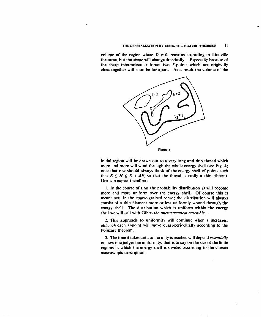
volume of the region where D 6 0, remains according to Liouvillethe same, but the shape will change drastically. Especially because ofthe sharp intermolecular forces two 17-points which are originallyclose together will soon be far apart. As a result the volume of the
Figurc 4
initial region will be drawn out to a very long and thin thread whichmore and more will wind through the whole energy shell (see Fig. 4;note that one should always think of the energy shell of points suchthat E _-• H =< E + JE, so that the thread is really a thin ribbon).One can expect therefore:
I. In the course of time the probability distribution D will becomemore and more uniform over the energy shell. Of course this ismeant on/y in the coarse-grained sense; the distribution will alwaysconsist of a thin filament more or less uniformly wound through theenergy shell. The distribution which is uniform within the energyshell we will call with Gibbs the inicrocanonical ensemble..
2. This approach to uniformity will continue when t increases,although each F-point will move quasi-periodically according to thePoincare theorem.
3. The time it takes until uniformity is reached will depend essentiallyon how one judges the uniformity, that is io say on the size of the finiteregions in which the energy shell is divided according to the chosenmacroscopic description.
12 THE EXPLANATION OF THE LAWS OF THERMODYNAMICS
4. For any macroscopic description there comes a time when theprobability of each macroscopic state is determined by the size of thecorresponding region of the energy shell. Since for large N, there isone region which is overwhelmingly the largest this will then also bethe most probable state and it characterizes the thermal equilibriumof the system.
I hope I have made clear the similarity between the Boltzmannpicture and the more general argument of Gibbs. Of course in bothcases a number of statements were made without proof, and they mayseem so vague that they are not amenable to proof! It is therefore ofgreat interest that at least part of the argument can be formulatedmuch more precisely by means of the Birkhoff ergodic theorems.'Let me remind you of these theorems:
(a) For a bounded mechanical motion and for any phase functiony = t(P) which is integrable over the energy surface, the time average:
(16) 7Lim I dtf(P,)
almost always exists. Here P, denotes the phase point which evolvesfrom the initial point P, by the motion. Furthermore T is independentof the choice of the initial point on the trajectory, but -v can vary withthe trajectory.
I will not try to indicate the proof since it is quite tricky. All thatis used is the boundedness of the motion and the Liouville theorem.It is therefore certainly applicable to the Gibbs macroscopic variables
(b) For a metricallyv transitive system the time average (16) is inde-pendent of the trajectory chosen and is equal to the ensemble average
(17) y, f ... f d~f(P)a H).
Here the integral goes over the energy surface and c(H) is the dis-tribution over the energy surface which corresponds to the uniformdistribution in the energy shell, so that:
const.(18) ,((1) - Igrad HIwhere the constant is to be determined by the normalization con-dition:
f... f a(//) d2 = 1.
a(H) is called the microcanonical surface distribution.

THE GENERALIZATION BY GIBBS. THE ERGODIC THEOREMS 13
A mechanical system is metrically transitive if the energy surfacecan not be divided into two finite regions such that the orbits startingfrom points in one of the regions always remain in that region. It isclearly a more precise formulation of the idea that in course of timethe path of the P-point will fill the whole energy surface which weused in the Boltzmann-Gibbs argument.' Of course it is very difficult(and it has not been achieved) to prove for a given Hamiltonian thatthe motion is or is not metrically transitive, and even examples whichcan be discussed exactly are rare.' However, the advantage of aprecise formulation remains. Note still that in principle it is notnecessary for the equality of the time and phase averages that themechanical system has a large number of degrees of freedom, althoughit seems more likely that the system will be metrically transitive ifN is large.
Let us now return to the Boltzmann-Gibbs picture of the approachto equilibrium. First, by taking in (16) and (17) forf(P) the character-istic function of a region A on the energy surface (that is f(P) = I ifP is inside A and f(P) = 0 otherwise), it follows that for a metricallytransitive system:
(19) Lim -t(A) = V(A)'.. T V
where t is the time the phase point spends in A, and where V(A) isthe volume of the part of the energy shell, whose total volume is V,which is based on A. This is clearly the precise formulation of theassumption essential for the Boltzmann picture that the time t(A) ismainly determined by the magnitude of the area of A. 10
Also the argument of Gibbs can now be expressed more precisely.The assumption that for large N there is one set of values of themacroscopic variables y, which correspond to by far the largest partof the energy surface, can be replaced by the requirement that thevariables yv must be normal variables."1 By this we mean that forlarge N the Y, must have the property:
(20) 1 ý.2,> - "
or in words: the fluctuation of each of the y, must be very smallcompared to .'•', itself. Here the average values are always taken asin (17) over the microcanonical ensemble. It is then clear that if
14 THE EXPLANATION OF THE LAWS OF THERMODYNAMICS
one starts at t = 0 with the initial distribution D(P, 0) the expectationvalues of the variables y, defined by:
(21) y,(t) = f ".. f d f(P)D(P, t)
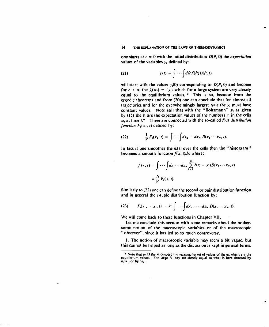
will start with the values ),(A) corresponding to D(P, 0) and becomefor t -,- x the fY(oo) = /y,) which for a large system are very closelyequal to the equilibrium values."2 This is so, because from theergodic theorems and from (20) one can conclude that for almost alltrajectories and for the overwhelmingly largest time the y, must haveconstant values. Note still that with the "Boltzmann" y, as givenby (15) the ., are the expectation values of the numbers n, in the cellsw, at time t.* These are connected with the so-called first distribution
function F,(xi, t) defined by:
(22) -F,(x1, t) = ... fdx 2 ." dxN D(x1 "xN, t).
In fact if one smoothes the AP(t) over the cells then the "histogram"becomes a smooth function f(x, t)dx where:
p p N
f (x, t) ... fdx .. dx,, (x - xi)D(xl xN, t)1=!
NV F,(x, t).
Similarly to (22) one can define the second or pair distribution function
and in general the s-tuple distribution function by:
(23) b,(.v , ,.-,, t) = P f. - f dx, fI .dXN D(X1 . XN., t)
We will come back to these functions in Chapter VII.Let me conclude this section with some remarks about the bother-
some notion of the macroscopic variables or of the macroscopic"observer", since it has led to so much controversy.
I. The notion of macroscopic variable may seem a bit vague, but
this cannot be helped as long as the discussion is kept in general terms.
* Note that in §3 the ,i, denoted the nwximnizing set of values of the ni, which arm theequilibrium values. For large N they are closely equal to what is here denoted byfi,(r) or by Ln,
THE GENERALIZATION BY GIBBS. THE ERGODIC THEOREMS 15
In Chapter Vii we shall see that the expectation values of the usualmacroscopic variables (as stress tensor, temperature distribution, etc.)can be found from the first few of the distribution functions (23).
2. There is an element of arbitrariness in the concept of the macro-scopic description of the system, which may seem objectionable.However, it is clear that in principle the macroscopic knowledge ofthe state of the system depends so to say on the zeal of the observerand can therefore not be defined in general. All one can say is thatthe macroscopic description is a contracted description, which usesmuch fewer variables than required for the precise microscopic speci-fication. Also, in practice, it usually is clear what the macroscopicvariables are, since they are dictated by the experimental phenomenawhich one tries to explain. To avoid the arbitrariness by introducingthe concept of a probability distribution over all possible macroscopicobservers,"3 as some authors have done, seems to me only to increasethe confusion.
3. The arbitrariness of the macroscopic description affects the timerequired for the expectation values Y,(t) to reach their equilibriumvalues 'y,>, since the choice of the y, determines the size of the regionsin which the energy shell is divided. One expresses this often by sayingthat the relaxation to equilibrium depends on the coarse graining.I think this is surely the case, but on the other hand it is clear that therelaxation to equilibrium will also depend on the Hamiltonian, that ison the structure of the mechanical system, and it is this dependence inwhich one is usually more interested, since the choice of the Y, isfixed by the experimental situation.
4. The variation in time of the yJ(t) in principle will always dependon the initial probability distribution D(P, 0) in r-space. This againseems objectionable, because of the arbitrariness. Even if one saysthat D(P, 0) should be chosen so as to correspond with our initialmacroscopic knowledge of the system, it is clear that this cannotpossibly determine D(P, 0) completely. The answer is, I think, thatone is only interested in that part of the relaxation of the *v, to equili-brium which is independent of the choice of D(P, 0). One shouldexpect that in a proper macroscopic experiment this will be the caseafter a short "chaotization period". Or one can say that after such ashort period the temporal development of the yv will be determinedby the y, themselves through equations which are of the first order intime. I call this the requirement of macroscopic causality. It is acondition on the choice of the macroscopic description, which clearly
16 THE EXPLANATION OF THE LAWS OF THERMODYNAMICS
can only be fulfilled in some asymptotic sense. We will come backto this in Chapter VII.
5. The laws of thermodynamics. We must now discuss the connec-tion with or the "explanation" of the laws of thermodynamics. In
the usual formulation of these laws, this means that we have toexplain the following five basic facts and notions.
(a) The existence of thermodynamic equilibrium for a closed system.This is the so-called zeroth law referred to in §3."1 Let me assumethat it was sufficiently elucidated in the previous sections!
(b) The notion of temperature. In thermodynamics the equili-brium is in the first place characterized by the temperature. In orderto represent the temperature by a number one must show besides theexistence of an equilibrium state, that the equilibrium state has thetransitive property. If system A is in equilibrium with the systemsB and C separately then B and C are also in equilibrium betweenthemselves. Here we mean by equilibrium of two systems the factthat the macroscopic properties of the systems will not change whenthe systems are coupled "weakly" together. The coupling mustallow interchange of energy between the systems, but the interactionenergy must be completely negligible compared to the energy of eachof the two systems.
(c) The first law of thermodynamics. Since the molecular model isalways taken to be a conservative mechanical system, so that the totalenergy is already conserved, the only question which remains is that of thedistinction between the notions of quantity of heat and of external work.
(d) The second law of thermodynamics for reversible phenomena.Knowing how the temperature T and the quantity of heat Q have tobe interpreted, one must show that for a "reversible" change of themacroscopic state SQ/T is a perfect differential of a function (theentropy) of the macroscopic state of the system.
(e) The second law of thermodynamics for irreversible phenomena.This says that in an irreversible or spontaneous change from oneequilibrium state to another (as for example the equalization oftemperature of two bodies A and B, when brought in contact) theentropy always increases.
In the following we will discuss these points in succession.
6. The notion of temperature. The canonical ensemble. For theintroduction of the notion of temperature we have to discuss theequilibrium of the system A under consideration when it is weakly
THE NOTION OF TEMPERATURE. THE CANONICAL ENSEMBLE 17
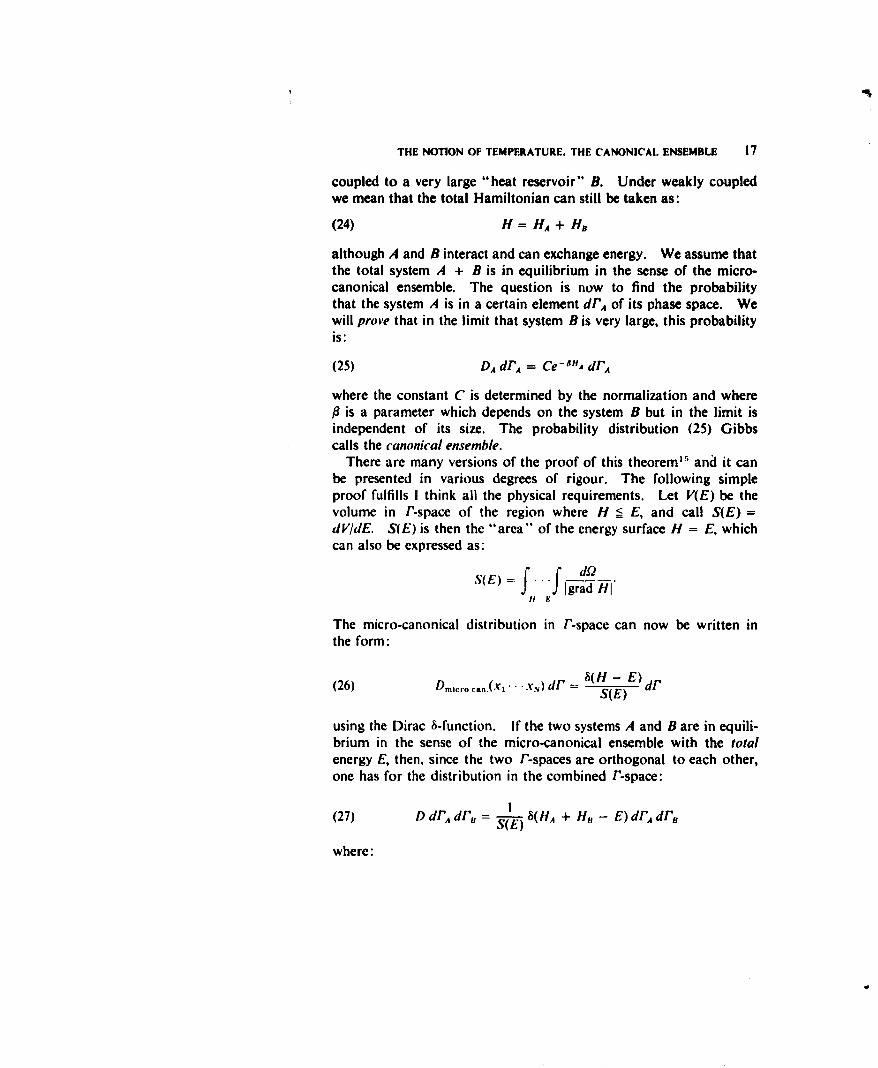
coupled to a very large "heat reservoir" B. Under weakly coupledwe mean that the total Hamiltonian can still be taken as:
(24) H= HA+ HB
although A and B interact and can exchange energy. We assume thatthe total system A + B is in equilibrium in the sense of the micro-canonical ensemble. The question is now to find the probabilitythat the system A is in a certain element dfA of its phase space. Wewill prove that in the limit that system B is very large, this probabilityis:
(25) DAdIA = Ce-'HA dFA
where the constant C is determined by the normalization and whereP is a parameter which depends on the system B but in the limit isindependent of its size. The probability distribution (25) Gibbscalls the canonical ensemble.
There are many versions of the proof of this theorem"5 and it canbe presented in various degrees of rigour. The following simpleproof fulfills I think all the physical requirements. Let V(E) be thevolume in r-space of the region where H < E, and call S(E) =dV/dE. S(E) is then the "area" of the energy surface H = E, whichcan also be expressed as:
f fIgrad HIII E
The micro-canonical distribution in P-space can now be written inthe form:
(26) Dmicro .. n.(x.' xs) dF S(H - E) dS(E)
using the Dirac 8-function. If the two systems A and B are in equili-brium in the sense of the micro-canonical ensemble with the totalenergy E, then, since the two P-spaces are orthogonal to each other,one has for the distribution in the combined P-space:
(27) D dl'Adl' = S(JE 8(HA + Ho - E) dFAdr,
where:
18 THE EXPLANATION OF THE LAWS OF THERMODYNAMICS
(28) S(E) = f, de SA(E)SB(E - E)
as follows immediately from the normalization. The distributionfunction for system A irrespective of the state of B is therefore:
DAdrA= (-) dri 8(HA + H, - E)
dIA(29) E de S(E)8(HA + HB- E)
SB(E- HA)drA.S(E)
In most proofs, to make things definite, one assumes that B consistsof a large number of weakly coupled systems, so that in turn
H = HI+H 2 +'" + H,.
Physically this means that one assumes the heat reservoir B to be anideal gas. and there is clearly nothing against that. But then we mayas well assume that B is an ideal gas of N point molecules, in whichcase:
H, = •..N-- 2m
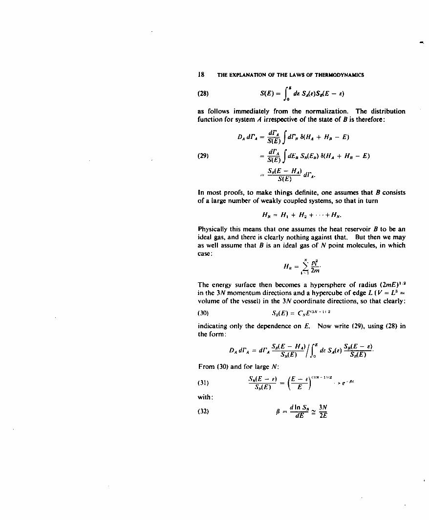
The energy surface then becomes a hypersphere of radius (2mE)I'2in the 3N momentum directions and a hypercube of edge L (V = L3 =volume of the vessel) in the 3N coordinate directions, so that clearly:
(30) St(E) = CNE 3N)- 1) 2
indicating only the dependence on E. Now write (29), using (28) inthe form:
DA arA = dPA S,(E - HA)/ dSA(E) S -E -
Dfd(Ae) oddr)S(E)
From (30) and for large N:
(31) S,(E - E) -(_f)N-I)!2SR(E) (E)
with:
(32) dlnS.~ 3NdE =2E
THE FIRST LAW OF THERMODYNAMICS 19
in which all that is assumed is that we are interested only in values ofe '4 E. Since DA is constant on energy surfaces HA = E one gets:
(33) DAdrA = drA e-HAo d SA(E)e-0'
which is of the form (25) and which is automatically normalized toone, since:
f... f rrADA(H) = f dE AFDi)
Note that I/# is proportional to the average energy per particle ofthe heat reservoir and is in this sense independent of the "size" ofthe reservoir.
Note that if we had several systems A,, A2..• each coupled to thevery large reservoir B, then the probability for each of them to be intheir region drAl is given by the canonical distribution with the sameft. The quantity P has therefore all the required temperature propertiesand it must be an universal function of the thermodynamic tempera-ture.
Note, finally, that the system A will always be canonically distri-buted, whatever its size. It could consist of a few or even one mole-cule. However, we will only use the theorem in the case that A is ofmacroscopic size. In this case because of the steepness of increaseof SA(E) with E, the canonical distribution (33) will be very narrowaround the average value, so that then the difference between thecanonical and the micro-canonical distribution will be slight."6
7. The first law of thermodynamics. Since both in the first and inthe second law of thermodynamics one considers changes of themacroscopic state of the system, we first need to look more closelyat the outside potential U in the Hamiltonian (1) through which thechanges of state are produced. In general one can say that thispotential U(r,, a,, a2 ... ) will depend, besides on the position r, ofthe ith molecule, on a number of parameters ak which characterizethe outside fields. Suppose for instance that the outside field isproduced by m fixed and independent centres of force. Then:
U(r,, a,, a 2 '.) = O 0j(1r1 - RkI)k=1
and the parameters a, are the positional coordinates Rk of the centres.
20 THE EXPLANATION OF THE LAWS OF THERMODYNAMICS
The force on the ith molecule:
(34) F1 = - ( )R k fd
is equal and opposite to the sum of the forces:
(35) kiXk = - cont.k I I1X k =E I O onst
exerted by the ith molecule on the centres as required by Newton'sthird law.
Although it is always possible to describe the outside force fieldsin such detail that the equality of action and reaction is put in evidence,it is in general not convenient to do so. Already if the force centresRk are not independent but are rigidly connected to each other, thenit is clearly indicated to describe the centres by the six coordinates ofthe rigigAstructure of connected sources. In this case the force F1on the ith molecule is still related to the generalized force:
(36) X, = - (iJU 0 h, it.
acting "in the direction ak" on the sources, but the relation is morecomplicated than in (34) and (35). In the general case we will there-fore not bother with the relation between the force:
F = - 4k COSt
acting on the ith molecule and the generalized force X, in the directiona,. The forces Xk will determine the work done on the gas forfixedconfiguration of the molecules if one changes the outside force fieldsby changing the parameters ak. In fact this work will be given by:(37) SW = - X, Sa, - X, Sa, ....
where the equality of action and reaction is used implicitly.Turning now to the first law of thermodynamics, I have remarked
already that since conservation of energy is so to say built into thetheory the only question remaining is how to distinguish between theexternal work W done on the system and the quantity of heat Q putinto the system.
Work can only be done on the gas by changing the parameters ak,
and from (36) and (37) we see that the work done on the gas is:
(38) 8W= -- k&1kk
THE SECOND LAW OF THERMODYNAMICS 21
where:
(39)T, f fd "HD
is the force in "direction" ok averaged over all the configurations of thegas. If one takes for D the microcanonical distribution then clearly8W must be equal to the increase SE of the energy, or in thermo-dynamical language the change 8 is then an adiabatic one. If, how-ever, one takes for D the canonical distribution, then after the change8ak of the parameters a, the original distribution will in general notbe an equilibrium distribution with respect to the heat reservoir.A redistribution will take place, which will change the average energy,and we will define the quantity of heat 8Q put into the system by:(40) SQ = 8E- 8W.That this is appropriate can be seen also by saying that the averageenergy can also be changed by changing the / of the heat reservoirwithout changing the parameters ak, and in this case the change shouldclearly be called the heat put into the system.
Note finally that since usually the only outside potential we consideris the wall potential for which there is only one parameter a, namelythe volume V of the vessel, one can write in this case Eq. (38)
W= -pSVwhere:
(41) p =f ... fd(-H ')D
is clearly the pressure exerted by the gas which if D is the canonicalensemble will be a function of V and f. The macroscopic state of thesystem is then specified by V and /, or in the general case by P and theparameters ak.
8. Tbe second law of tbermodynamics. We will now show that for achange 8 in which both the 9 of the heat reservoir and the parametersa, are changed in such a slow or "reversible" way that the systemmay always be considered to be canonically distributed, the quantityP8Q is a perfect differential of a function of the state of the system,that is a function of P and the ak.
To prove this, write the average energy in the form:
f= r Hei - lnZ
J dre-l"
22 THE EXPLANATION OF THE LAWS OF THERMODYNAMICS
with:
(42) Z = fPre-OH.
Hence:
S - a2 02ý= 5 (In Z) SP - ýp- (in Z) Sak.
From (38) follows that the work done on the system can be written as:
fdIe- OH -OH Sa8 W = Jdea l8an 8ksw - fýa-, _I :ElIn Z Sf dr = - k O ak .
Therefore:
P SQ =P(8R- 8W);)
2 1 nZ 02a nZ alnz].8a=-i- k TPa• a aa
i)[, In _Z IZa[ ' nZ a
=8[InZ - P t In Zj = [-P2 (Ilnz)Z
which concludes the proof.
Comparison with SQJT = 8S shows that:
(44) P = k -T
S = -kp2 I(nZ + const.
(45)= -jT(kTInZ) + const.
where T is the absolute thermodynamic temperature, S the entropyand k an universal constant which cannot be determined from thisargument. To find k, one must consider the case of an ideal gas,enclosed in the volume V. Then:
Z= f(... f )dri ...drf...fdpl...dpNexp(-P
= V,(21rmkT)3 1112.
THE SECOND LAW OF THERMODYNAMICS 23
From (41) this gives for the pressure:8 NkT
(46) p = b (kT In Z) = AT
So one gets the ideal gas law if k = RIN is the gas constant permolecule.
I will omit a more detailed discussion about the question in whichprecise sense the entropy S as defined by (45) has also the property(required by the second law for irreversible processes) of increasingin any spontaneous transition from one equilibrium state to another.Since we have explained the zeroth law the reader will believe thatthis part of the second law, which is a more precise expression of theirreversible behaviour of macroscopic systems, can be "explained"in a similar way.
Finally a remark about the constant in the equation (45) for theentropy. Clearly from the argument given it is not possible to fixthis constant and one cannot even determine its dependence on thenumber of particles N. Thermodynamically only entropy differencesbetween states which can be connected by a reversible transition areoperationally defined. Therefore since N is fixed, the dependence ofthe entropy on N can only be agreed upon by convention."7 How-ever, it certainly is a sensible convention to require that the entropyat fixed Tand for large N and large V, so that r = V/N is fixed, becomesof the form:
(47) S = Ni?(r, T).
The entropy becomes then a so-called extensive variable, that is pro-portional to the size of the system when the intensive variables T and vare given. In addition one also would like to insure that all theclassical results agree in the limit T ,. o with the results of thequantum statistics, if one makes the usual assumption that each non-degenerate energy level has the statistical weight equal to one. Notethat this is of course also a convention, since only the ratios of theweights of different levels have operational meaning, but it certainlyis a very appealing convention. Both these objectives are realized byomitting the constant in (45) and by defining Z instead of by (42), by:
Z(V, T, N) = 3N fdre- "1
(48)
NI!A3N fkx( < )
24 THE EXPLANATION OF THE LAWS OF THERMODYNAMICS
where h is Planck's constant, A = h/(2wmkT) 12 , and where in the secondline the integration over the momenta has been carried out. Z iscalled the partition function. Comparison with the thermodynamicformulas then shows that:
(49) W(V, T, N)= -kln Z
is the (Helmholtz) free energy, from which all other macroscopicquantities follow. Especially:
(50)W '
R=V'T- C T,= Or'
and so on. In Chapter 11 we will show that for large N and V,v = VIN fixed:
(51) WP(V, T, N) = N#(v, T)
from which (47) follows.
NOTES ON CHAPTER I
1. For a critical discussion of the foundations of statistical mechanicsthe article of P. and T. Ehrenfest (Begriffliche Grundlagen der Statis-tischen Auffassung in der Mechanik, Enzyclopidie der Math. Wiss.Vol. IV, Art. 32, 1912), is still indispensable. It is now also availablein English translation (by M. J. Moravcsik, Cornell University Press,1959). For a recent account and for the recent literature see forinstance A. M uinster, Prinzipien der Statistischen Mechanik, Handbuchder Physik, Vol. 111/2, 1959.
The difference in attitude with respect to the foundations is forinstance illustrated by the fact that a mathematician (e.g. Khinchin,see his book: Mathematical Foundations of Statistical Mechanics,translated by G. Gamov, Dover reprint, 1949), is inclined to lookupon the ergodic theorems of Birkhoff e.o. as the proper basis forthe theory, while a physicist is often inclined to think that thesetheorems are either almost obvious or not really essential. This is forinstance the view expressed by Landau and Lifshitz in their excellentbook Statistical Physics (Pergamon Press, London, 1958). Theseauthors start from the beginning not with a closed system, but with asystem interacting with a large heat reservoir. Other physicists (e.g.Tolman in his well known book, The Principles of Statistical Mechanics(Oxford, 1938)) more or less postulate the microcanonical ensemble asthe representation of a closed system in thermal equilibrium. It istrue that in either of these two ways one can avoid the vexing problemof the approach to equilibrium while one keeps all that is needed forthe treatment of the problems of the equilibrium theory. However,it seems to us that the goal should be an unified treatment of bothequilibrium and non-equilibrium statistical mechanics. To do this,one cannot avoid the ergodic problem, and the Birkhoff ergodictheorems then become an important first step, which however does notexhaust the subject!
2. The assumptions of a hard core and of a finite range are onlymade in order to have a definite mathematical model for the inter-molecular potential. From the quantum theory of the van derWaals' forces between neutral molecules it only follows that at shortdistances one has a very sharp repulsion while at larger distances
25

26 THE EXPLANATION OF THE LAWS OF THERMODYNAMICS
there is an attraction which goes to zero as I/,r. Since the theorydoes not give an explicit expression for 0(r) it is customary to usesimple semi-empirical formulas, as fo6r instance the so-called Lennard-Jones (12, 6) potential: (I ,I(a) 4(r) = 4 I J(r/)12 (rl/')6which represents the two features of 0(r) which the quantum theorypredicts. We will come back to this in Chapter i1.
3. The theorem of Liouville proves that the volume in phase-spaceis a so-called integral invariant of the motion. It is well known thatthe volume is only one of a series of such integral invariants whichwere discovered by Poincare. One can prove that for any ensembleflow and for any s such that I < s < n:
(b) D f f dq,1 dp,1 dqI dp424 dq.. dp. = O.
In here the integral goes over a 2s-dimensional surface and the sumgoes over all ,C, different combinations of the indices i,. • .. Eq. (b)states that the integral does not change if one moves with the fluid.For s = n Eq. (b) becomes the Liouville theorem in the Lagrangianform. Compare E. T. Whittaker, Anab'tical Dynamics, 4th ed.(Cambridge University Press, Cambridge, 1960), Chapter 10, or for amore succinct discussion H. Goldstein, Classical Mechanics (Addison-Wesley Press, Cambridge, Massachusetts, 1950), pp. 247-250.
One might well ask the reason why the particular case of (b) repre-sented by the Liouville theorem plays such a special role in statisticalmechanics. We think the simple answer is that the Liouville theoremis the only invariance theorem which affects the change of the densityp. Only for singular density distributions, in which the members ofthe ensemble would be distributed over surfaces of dimensionalityless than 2n, would the more general invariance properties (b) be ofimportance.
4. Proof of the Poincar6 recurrence theorem. We follow thepresentation by M. Kac in the Boulder lectures of 1957 (Probabilityand related topics in physical sciences, p. 63). Let A be the region onthe energysurface H = E around the initial point P (see Fig. 2). Ifwe follow all the points of A in their motion, then it is easy to showthat:
(c) I(A) = f fIgrad HIA
NOTES ON CHAPTER 1 27
remains the same. To see this, consider two energysurfaces H = Eand H = E + JE. If Jn is the normal distance between these twosurfaces, then according to Liouville the cylindrical volume:
will be conserved. Since JE = Igrad Hldn and 4E is fixed thisimplies that (c) remains constant. Call IA(A) the measure of the regionA. This is therefore a positive and finite number associated with Awhich is conserved in the streaming over the energysurface. Sincethe total area of the energysurface is finite because of the boundednessof the motion also the total measure of the energysurface will be finite.
Suppose now that there are points in A which in their motion wouldnever come back to A and that there are so many of such points thatthey would fill a subregion B in A, which has a finite measure. Wewill prove that this is impossible. Follow namely the region B in itsmotion and consider the corresponding regions B,, B 2,... occupiedby the points of B at the later times 4, 24A ... If J is chosen largeenough so that B and B, do not overlap it follows that none of theregions B, B1, B2,, overlap. To see this note that if say B, andB,., A had points in common, then from the unicity of the motion (theimpossibility of the crossing of two streamlines) it follows by tracingthe motion backwards that also B, -, and B,. A, - must have pointsin common. Continuing this argument one would end up with thestatement that B itself must have points in common with B4, whichmeans that B contains points which after the time k4 would havereturned to A. But this is contrary to the supposition that B is aregion containing all points which never come back. If the regionsB, B,, B2', - do not overlap, then since p(B) = pA(B1 ) = IA(B2 ) =.
the total measure of all these regions would be infinite, which isimpossible since the measure of the total energysurface is finite.Hence one concludes that the measure of all points in A, which willnever return to A must be zero, which is the Poincar6 theorem.
5. The proof can be given with various degrees of precision. Thesimplest way, following Boltzmann and Tolman (Principles of Statis-tical Mechanics, p. 79) is to take the logarithm of W and to apply theStirling approximation in the weak form:(d) log in! = it log n - it.One then gets:
(e) log W = NlogN - nnlogn, + >n, logto,.
28 THE EXPLANATION OF THE LAWS OF THERMODYNAMICS
Varying the n, by An, one obtains:
( C) lo g W + .W . n ,( - lo g n , - I + lo g - + . . . .
W 2 n
The An, have to fulfill the subsidiary conditions:
A4n, = 0 E, End, = oi I
because N and E are given. Multiplying these conditions with theLagrange multipliers (log A + I) and (-Pi) respectively, and addingthe result to (f), one sees that the first variation vanishes for the setfulfilling the conditions:
-lognt, + logA + log w l,- = 0or:
fi, = Aw, e-fi,.
That for this set W is a very sharp maximum follows from (f) since forthis set:
SW+ AW I 2. _ n,2(g) o - Ný (4n11,,) 2>av
if W is the value of W for nt = n,. Clearly if N is very large theneven a very small average relative deviation '4 n/i,' from the A, willreduce the corresponding volume enormously.
From this proof we see that a more correct statement of the theoremis that the M.B. distribution, together with those states for which
occupy almost all of the energy shell.
6. Requirement (a) expresses the property that any macroscopicdescription must have, namely that it must be insensitive to smallchanges in the position of the phase point P. That such a "coarsegraining" of the P-space is necessary for the whole argument wasespecially emphasized by P. and T. Ehrenfest (I.c. Note I). Onemay say that this coarse graining depends on the observer through hischoice of the macroscopic variables. On the other hand (b) can belooked upon as the requirement imposed by the system (mainlybecause of the fact that N is very large) on the choice of its macro-scopic description.
NOTES ON CHAPTER I 29
7. See Khinchin, Statistical Mechanics, Chapter 11, §5, or E. Hopf,Ergodentheorie (Berlin, 1937), or P. R. Halmos, Lectures on ergodictheory (Publications of the Mathematical Society of Japan, no. 3,1956), also for the further mathematical literature. In the followingthe word "almost" means as usual "except possibly for a set ofmeasure zero".
8. In the physical literature the same idea is expressed by sayingthat the system must be quasi-ergodic. (See P. and T. Ehrenfest,i.e., also for the discussion and criticism of the older ergodic hypo-thesis of Boltzmann.) By this one means that the trajectory startingfrom almost any point P will cross in the course of time any regionaround any' point Q of the energysurface. A metrically transitivesystem is obviously quasi-ergodic, but the inverse is not necessarilytrue. It may be that the energysurface can be divided in two setsboth of finite measure and so interwoven that the points in each setare everywhere dense on the surface. If the orbits starting from pointsin one set stay in that set then the system is clearly not metricallytransitive although it is obviously quasi-ergodic. From the quasi-ergodic property Eq. (19) cannot be deduced. This was attemptedby A. Rosenthal (Ann. Physik 43 (1914) 894) and the error was pointedout by A. Melamit (Acta Phys. Polon. 1 (1932) 281).
9. The best known example is the motion of a mass point on asurface of constant negative curvature. That the flow defined by thegeodesics on such a surface is metrically transitive was first proved byG. A. Hedlund in 1934 (Ann. of Math. 35 (1934) 787). Comparealso E. Hopf, Ergodentheorie, Chapter V, and for a simplified proofG. A. Hedlund, Amer. J. Math. 62 (1940) 233.
There is also a paper by Fermi (Physik. Z. 24 (1923) 261) in which aproof is presented of the quasi ergodicity of so-called canonical normalsystems with more than two degrees of freedom. These systems wereconsidered by Poincard (Les Methodes Nouvelles de la MecaniqueCeleste, Vol. i, Chapter 5) and they are essentially non-degeneratemultiply periodic systems which are perturbed by a potential which isperiodic in the angle variables. They include therefore a wide classof mechanical systems, and it would be of great interest to knowwhether Fermi's argument could be made into a rigorous proof ofthe metrical transitivity of these systems.
10. Eq. (19) is related to a theorem proved by M. Kac (Bull. Amer.Math. Soc. 53 (1947) 1002) about the average recurrence time. Con-sider again a discrete set of time points 4, 2,,... as in the proof of
30 THE EXPLANATION OF THE LAWS OF THERMODYNAMICS
the Poincar6 theorem (Note 4) and an area A on the energysurface.Let n(P),4 be the first time for a point P in A to return to A, so thatP, c A. Then for a metrically transitive system Kac proves that theaverage recurrence time defined by:
id = -.4 ..f-f n(P)A
is determined only by the area of A and in fact is equal to (VI V(A)) J.The smaller the area A is, the longer the average recurrence time willbe, and the shorter (according to Eq. (19)) the point will spend inthe area A.
11. The notion of a normal property of a system was introduced byJeans (Dynamical Theory of Gases, 3rd ed., 1921, p. 74), and wasfurther discussed by Fowler (Statistical Mechanics, Cambridge, 1929,§1.4, p. 8). We think that the definition used in the text expresses moreprecisely what these authors had in mind.
12. This can also be expressed in the following way. Since D(P, 0)corresponds to a given set of values yo, of the macroscopic variablesat t = 0, one finds by integrating D(P, t) over the different regions onthe energy shell corresponding to the different sets of values of theyi, the conditional probability P(jo, I.,, t) that at time t the macro-scopic variables have the values y, if at t = 0 they have the valuesy10,. For t - wo, P(.• 0
)jy,, t) '( Wy),Y2.. '), where W(O, Y2"'. ) isdetermiued by the volume of the energy shell corresponding to theset of values.i'•, ' ' -. Because for large N there is one set of valuesof the Y, corresponding to an overwhelmingly largest volume, thefunction W(y,y.. , .) will be very sharply peaked at this equilibriumset of values of the v,.
Formulated in this way the theory becomes completely similar tothe theory of stationary stochastic processes.
13. This was done first by J. von Neumann (Z. Physik. 57 (1929)80). For a discussion and criticism of this concept see the article byM. Fierz in the Memorial Volume to Wolfgang Pauli (IntersciencePublishers, New York, 1960).
14. It should be pointed out that this terminology is not generallyused. For instance R. H. Fowler and E. A. Guggenheim (StatisticalThermodynamics, Cambridge, 1939, p. 56) call the postulate of theexistence of temperature the zeroth law of thermodynamics. Since the
NOTES ON CHATER I 31
notion of temperature depends, besides on the existence of thermo-dynamic equilibrium, on the transitive property of the equilibrium state,and since for the statistical interpretation of the notion of temperatureone needs the canonical ensemble, it seems to us preferable to reservethe term zeroth law to the fundamental fact of the approach to equili-brium of a closed system.
15. See for instance: Boltzmann, Wissenschaftliche Abhandlungen,Vol. I, p. 284; G. Krutkow, Z. Physik. 81 (1933) 377; Khinchin,Statistical Mechanics, Chapter 5, §19; H. Grad, Comm. Pure Appl.Math. 5 (1952) 455.
16. It seems very likely therefore that for a system with a largenumber of molecules the macroscopic properties of the equilibriumstate can be obtained either from the canonical or from the micro-canonical ensemble and that the results will always be the same. Fromthe point of view of thermodynamics the difference between the twoensembles lies only in the choice of the basic thermodynamic character-istic function and in the corresponding choice of the macroscopicvariables. It is difficult though to prove this rigorously and in allgenerality, so that it should be verified for any specific problem.
17. This was pointed out clearly in the basic paper by P. Ehrenfestand V. Trkal (Ann. Physik. 65 (1921) 609). The neglect of this pointhas led to a great deal of discussion and to the so-called " N! " con-troversy. See for instance E. Schrodinger, Statistical Thermodynamics(Cambridge University Press, 1946) and 0. Stern, Revs. ModernPhys. 11 (1949) 534.
CHAPTER II
Theory of the Non-Ideal Gas
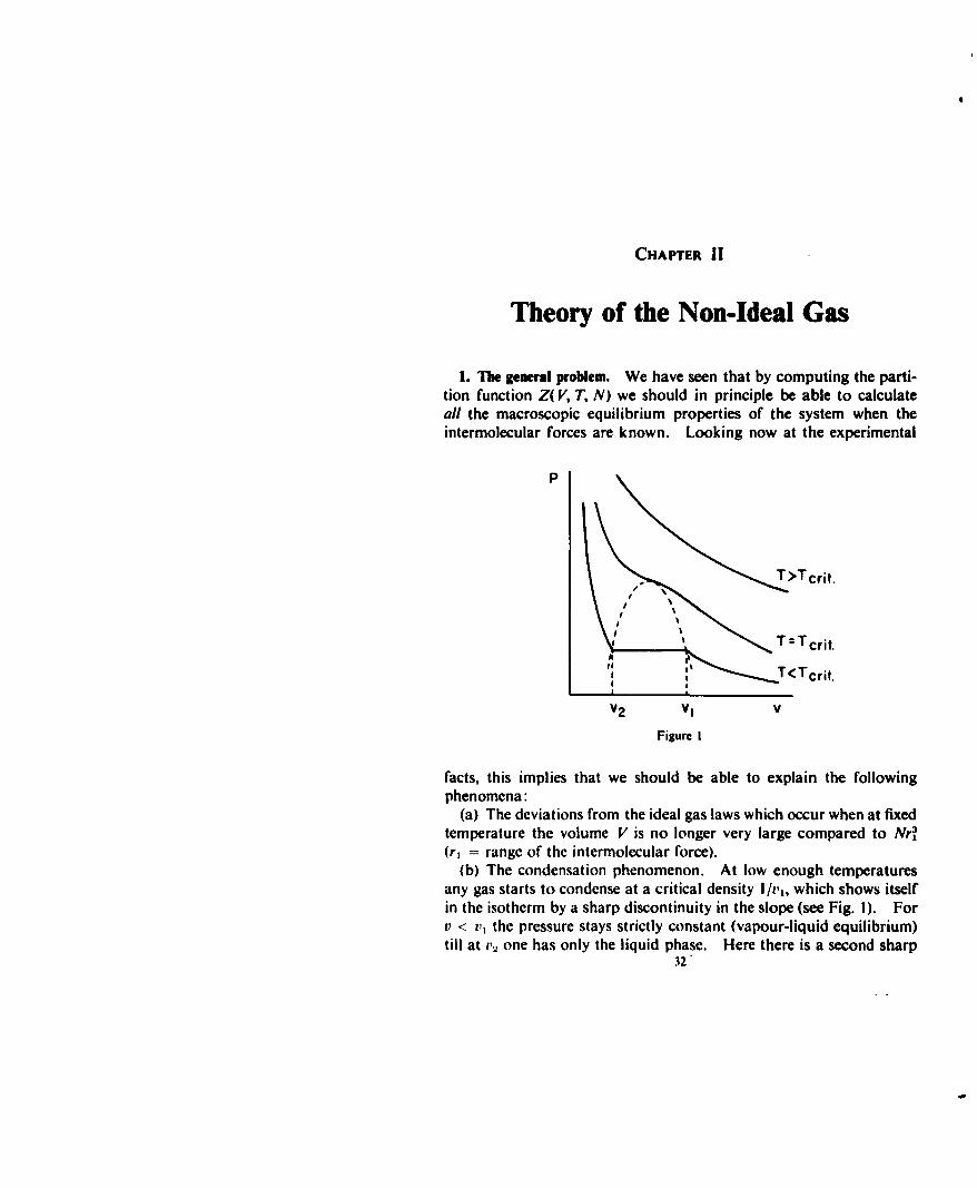
1. The general problem. We have seen that by computing the parti-tion function Z(V, T, N) we should in principle be able to calculateall the macroscopic equilibrium properties of the system when theintermolecular forces are known. Looking now at the experimental
P
S T>Tcrit.
I %
V2 V1 V
Figure I
facts, this implies that we should be able to explain the followingphenomena:
(a) The deviations from the ideal gas laws which occur when at fixedtemperature the volume V is no longer very large compared to Nr•(r, = range of the intermolecular force).
(b) The condensation phenomenon. At low enough temperaturesany gas starts to condense at a critical density I/t',, which shows itselfin the isotherm by a sharp discontinuity in the slope (see Fig. I). Forv < vl the pressure stays strictly constant (vapour-liquid equilibrium)till at r2 one has only the liquid phase. Here there is a second sharp
32
THE THEORY OF VAN DER WAALS 33
discontinuity in the slope of the isotherm, and for v < v2 the isothermrises steeply corresponding to the small compressibility of allliquids.
(c) The existence of a critical temperature T,,,,. Again for all sub-stances the condensation phenomenon only occurs for T < Tcrt. IfT approaches Tcrlt the horizontal portion of the isotherm becomesshorter and it disappears in the critical point C. For T > T,,,t thereis no longer a discontinuity in the isotherm.
There are other general phenomena. At still smaller volumes andprobably at any temperature the substance solidifies, and one has thecorresponding solid-liquid and solid-vapour equilibria.' But theexplanation of these phenomena from the basic integral (1, 48) forZ(V, T, N) is still so far from being accomplished that I will notbother the reader with other experimental facts. Before giving asummary of what has been accomplished, let us look at the historicalbackground.
2. The theory of van der Waals. The first great advance in theunderstanding of the properties of gases and liquids was made byvan der Waals in his famous Leiden dissertation of 1873. Van derWaals tried to take into account the effect of the intermolecularforce (attraction at large distance, sharp repulsion at short distance)on the equation of state of the gas and hc arrived at the famousequation:
(!) (p + -p)(V- b) = NkT
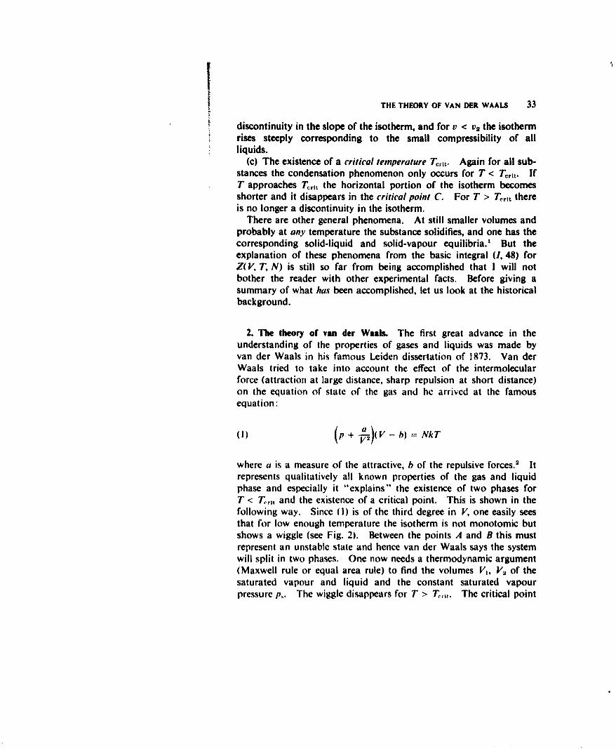
where a is a measure of the attractive, b of the repulsive forces.2 Itrepresents qualitatively all known properties of the gas and liquidphase and especially it "explains" the existence of two phases forT < Trj, and the existence of a critical point. This is shown in thefollowing way. Since (I) is of the third degree in V, one easily seesthat for low enough temperature the isotherm is not monotomic butshows a wiggle (see Fig. 2). Between the points A and B this mustrepresent an unstable state and hence van der Waals says the systemwill split in two phases. One now needs a thermodynamic argument(Maxwell rule or equal area rule) to find the volumes V1, V2 of thesaturated vapour and liquid and the constant saturated vapourpressure p.,. The wiggle disappears for T > T,,,. The critical point
34 THEORY OF THE NON-IDEAL GAS
C is fixed by the fact that there the isotherm has an horizontal inflexionpoint, so that:
gV = 0 - 0l
from which follows:a 8a
(2) V= 3b, pc = a R' = 8a
P
\CriticoI point
Tcrit.
Ps 5 I'
SA TTcrit.
V2 VI V
Figure 2
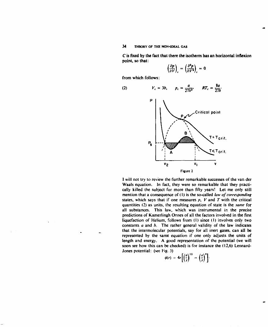
I will not try to review the further remarkable successes of the van derWaals equation. In fact, they were so remarkable that they practi-cally killed the subject for more than fifty years! Let me only stillmention that a consequence of (I) is the so-called law of correspondingstates, which says that if one measures p, V and T with the criticalquantities (2) as units, the resulting equation of state is the same forall substances. This law, which was instrumental in the precisepredictions of Kamerlingh Onnes of all the factors involved in the firstliquefaction of Helium, follows from (I) since (I) involves only twoconstants a and h. The rather general validity of the law indicatesthat the intermolecular potentials, say for all inert gases, can all berepresented by the same equation if one only adjusts the units oflength and energy. A good representation of the potential (we willsoon see how this can be checked) is for instance the (12,6) Lennard-Jones potential: (see Fig. 3)
0(r) = 4r[('- -()]
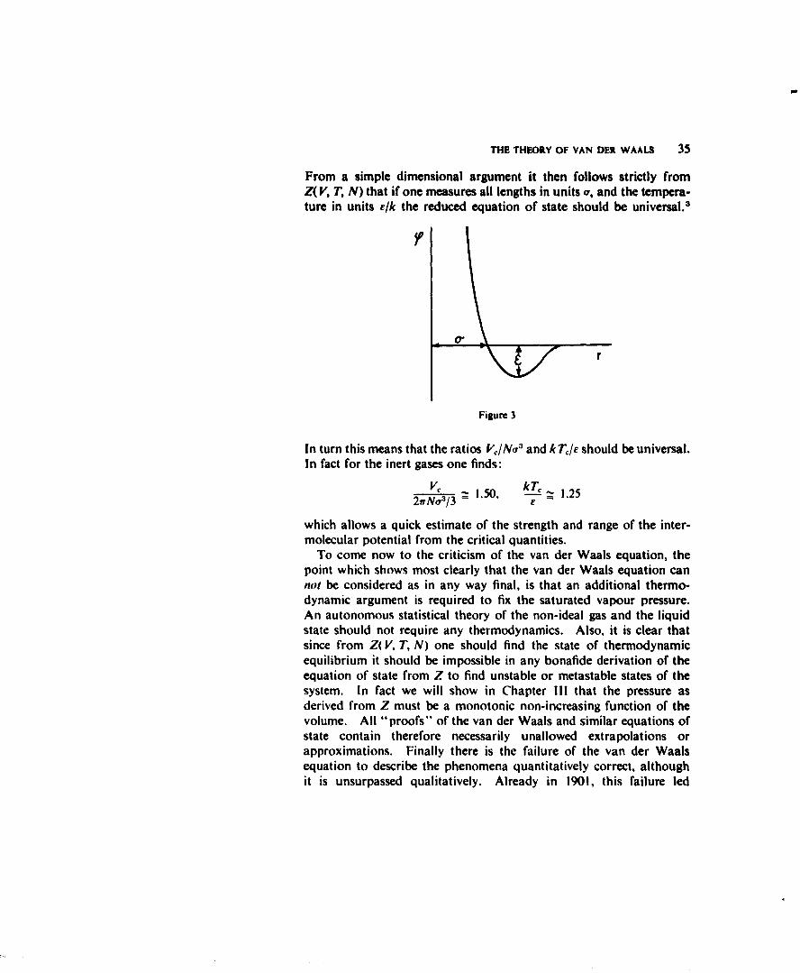
THE THEORY OF VAN DER WAALS 35
From a simple dimensional argument it then follows strictly fromZ( V, T, N) that if one measures all lengths in units a, and the tempera-ture in units e/k the reduced equation of state should be universal.
01
r
Figure 3
In turn this means that the ratios V/Noa and kTI./ should be universal.In fact for the inert gases one finds:
V, ~ kT,2•Na/ =1.50, - 1.25
which allows a quick estimate of the strength and range of the inter-molecular potential from the critical quantities.
To come now to the criticism of the van der Waals equation, thepoint which shows most clearly that the van der Waals equation cannot be considered as in any way final, is that an additional thermo-dynamic argument is required to fix the saturated vapour pressure.An autonomous statistical theory of the non-ideal gas and the liquidstate should not require any thermodynamics. Also, it is clear thatsince from Z( V, T, N) one should find the state of thermodynamicequilibrium it should be impossible in any bonafide derivation of theequation of state from Z to find unstable or metastable states of thesystem. In fact we will show in Chapter III that the pressure asderived from Z must be a monotonic non-increasing function of thevolume. All "proofs% of the van der Waals and similar equations ofstate contain therefore necessarily unallowed extrapolations orapproximations. Finally there is the failure of the van der Waalsequation to describe the phenomena quantitatively correct, althoughit is unsurpassed qualitatively. Already in 1901, this failure led
36 THEORY OF THE NON-IDEAL GAS
f(r)
-l
Figure 4
Kamerlingh Onnes to abandon all closed expressions for the equationof state and to represent the data by a series expansion of the form:
(3) -= I + -D + E(-T) +RT V V
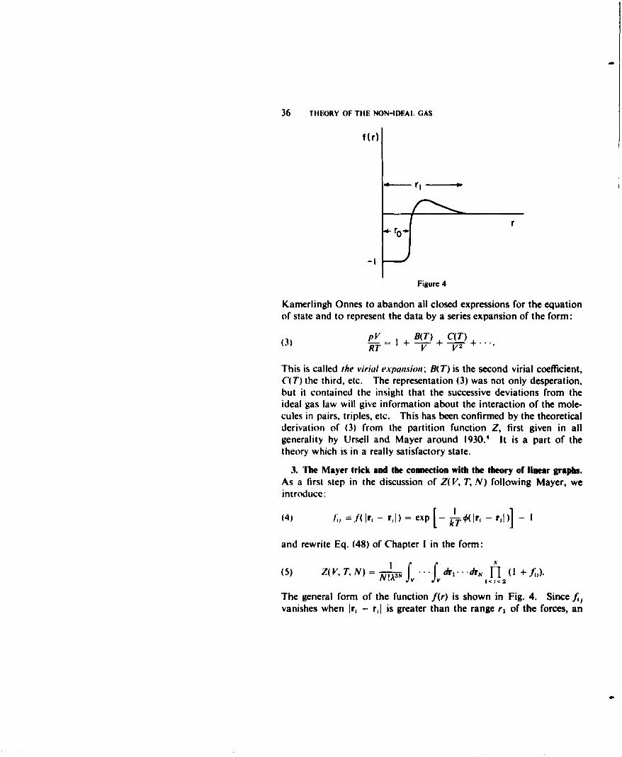
This is called the virial expansion, B(T) is the second virial coefficient,C(T) the third, etc. The representation (3) was not only desperation,but it contained the insight that the successive deviations from theideal gas law will give information about the interaction of the mole-cules in pairs, triples, etc. This has been confirmed by the theoreticalderivation of (3) from the partition function Z, first given in allgenerality by Ursell and Mayer around 1930.' It is a part of thetheory which is in a really satisfactory state.
3. The Mayer trick and the connection with the theory of linear graphs.As a first step in the discussion of Z( V, T, N) following Mayer, weintroduce:
(4, I, f(lr, - r,I)= exp [-_ 4IT r, - r,,)] -
and rewrite Eq. (48) of Chapter I in the form:
(5) Z(V, T, N) =1*1... drN H ( +f).
The general form of the function f(r) is shown in Fig. 4. Since fivanishes when 1r, - rj is greater than the range r, of the forces, an
THE CONNECTION WITH THE THEORY OF LINEAR GRAPHS 37
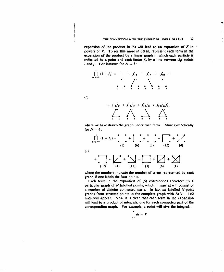
expansion of the product in (5) will lead to an expansion of Z inpowers of V. To see this more in detail, represent each term in theexpansion of the product by a linear graph in which each particle isindicated by a point and each factor fJ, by a line between the pointsi andj. For instance for N = 3:
3
H (l+;J)= I + J12 + A3 + f 23 +<1<-2ol / o
0 0 .\ 0 -------a
2 3 2 3 2 3 2 3
(6)
+ A1 2f24 + f 2f13 + fl 3f 23 + fzAJ 23f3 14L A A2 3 2 3 2 3 2 3
where we have drawn the graph under each term. More symbolicallyfor N = 4:
(I +J,) =: + + + +(!) (6) (3) (12) (4)
(7)
(12) (4) (12) (3) (6) (1)
where the numbers indicate the number of terms represented by eachgraph if one labels the four points.
Each term in the expansion of (5) corresponds therefore to aparticular graph of N labelled points, which in general will consist ofa number of disjoint connected parts. In fact all labelled N-pointgraphs from separate points to the complete graph with N(N - 1)/2lines will appear. Now it is clear that each term in the expansionwill lead to a product of integrals, one for each connected part of thecorresponding graph. For example, a point will give the integral:
dr= V
38 THEORY OF THE NON-IDEAL GAS
a line (i,j) the integral:
f, fv dr, drifil
a triangle (i, 1, k) the integral:
(8) fV f1 dr1 'kkflfkk
and so on. We will call a connected graph also sometimes a clusterand the corresponding integral like (8) a cluster integral. The advan-tage of such an expansion of the integrand in (5) is that because of theshort range of the forces (beyond which the fil are zero), the leadingterm of each cluster integral is proportional to V. It is this featurewhich has allowed Ursell and Mayer to derive the virial expansion (3)and to find explicit expressions for the virial coefficients in terms ofthe functions f,.
4. Some notions of the theory of linear graphs. Since we need someof the simple notions of the theory of graphs, and since part of theterminology I am used to is semi-private, let me collect here all thatwe will need.'
A linear graph is a collection of points with lines between certainpairs of points. In general there may be more than one line connect-ing two points and also loops may occur. If any two points areconnected by at most one line and if there are no loops we call thegraph simple (see Fig. 5). We will mainly have to deal with suchgraphs. A subset of points which are joined successively by lines iscalled a path connecting the initial and final point. If the final pointcoincides with the initial point we speak of a cycle. A connectedgraph is one in which there is at least one path between any twopoints. Otherwise the graph is disconnected. It is clearly sufficientto study connected graphs. An articulation point is a point where a
(a) (b)Figure 5. (a) simple graphs; (b) not simple graphs
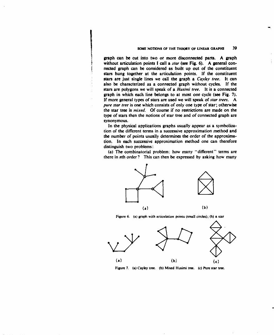
SOME NOTIONS OF THE THEORY OF LINEAR GRAPHS 39
graph can be cut into two or more disconnected parts. A graph
without articulation points I call a star (see Fig. 6). A general con-nected graph can be considered as built up out of the constituentstars hung together at the articulation points. If the constituentstars are just single lines we call the graph a Cayley tree. It canalso be characterized as a connected graph without cycles, If thestars are polygons we will speak of a Husimi tree. It is a connectedgraph in which each line belongs to at most one cycle (see Fig. 7).If more general types of stars are used we will speak of star trees. Apure star tree is one which consists of only one type of star; otherwisethe star tree is mixed. Of course if no restrictions are made on thetype of stars then the notions of star tree and of connected graph aresynonymous.
In the physical applications graphs usually appear as a symboliza-tion of the different terms in a successive approximation method andthe number of points usually determines the order of the approxima-tion. In each successive approximation method one can thereforedistinguish two problems:
(a) The combinatorial problem: how many "different" terms arethere in nth order ? This can then be expressed by asking how many
(b)(a) (b)
Figure 6. (a) graph with articulation points (small circles); (b) a star
(a) (b) (C)
Figure 7. (a) Cayley tree. (b) Mixed Husimi tree. (c) Pure star tree.
40 THEORY OF THE NON-IDEAL GAS
graphs of n points and of a specific type (as determined by the problem)there are.
(b) The integral problem: what is the contribution or the weightof each graph?
In the combinatorial problem one must distinguish between labelledgraphs and free (or topological) graphs. In a labelled graph differentpoints are distinguished by some index. In a free graph the pointsare regarded as not distinguishable. Of fundamental importance isthe number of different labelled graphs corresponding to a given freegraph. To enumerate the possibilities one needs the notion of thegroup of a graph. This is defined as the group of automorphisms ofthe graph, that is the group of the one to one correspondences of thepoints of the graph which leave the connections invariant. The groupcan be considered as a permutation group of the points. For example,for an n-gon the group is the dihedral group of order 2n, and for aso-called complete graph of n points (i.e., the graph where all pairs ofpoints are joined by lines) the group is the symmetric group of degreen. The order of the group is the symmetry number s of the graph.If one has a free graph of p points and symmetry number s, then thereare clearly p!/s different ways in which one can label the points so thatone obtains p!/s different labelled graphs.
5. The first Mayer theorem. We now return to the calculation ofthe partition function Z( V, T, N) as given by (5) and we will considerthat the product is expanded and that each term is symbolized by agraph of N labelled points as explained in §3. We also saw that theneach term becomes a product of factors each referring to a disjointconnected part of the graph. Mayer showed that the resulting sumof products can be put in a simple form. To derive this, it is illumin-ating to consider Mayer's result as a special case of the followinggeneral theorem."
THEORFM I. Consider the quantity FN defined by:
(9) F= W(GN)(GN)
where the sum goes over all graphs GN (connected or disconnected) withN labelled points, and where W(GN) is a "weight" which is a functionof the graph GN and which is supposed to have the properties:
(a) W(GN) is independent of the labelling of the N points, whichmeans that it only depends on the free graph.
(b) W(GN) CI W(C) where the product goes over all the disjoint
THE FIRST MAYER THEOREM 41
connected parts C, of GN.Introduce further the quantity:
(10) f, = W(C,)(C,#)
where the sum runs over all connected graphs with labelled points. Thetheorem then states that:
(II) I + F(x) = els)
where F(x) and f(x) are the generating functions of the quantities FNand f, defined by:
XIV(12) Fix) = F N W1,. ' f(x) f= F
The proof of the theorem depends on the following fundamentallemma, which we will use over and over again, so that we will formu-late and prove it in all generality.
PRODUCT THEOREM. Consider two arbitrary (finite or infinite)collections .) and N1 of free graphs and forrm the product collection.tx (4 which consists of all possible pairs of graphs one from .V andone from 01. Assign weights to each of the graphs in .t and oi, and
assign to each graph ofthe product collection the product of the weightsof the two graphs of which it is formed, if now we label the graphs in.J., (4 and .k x 05 in all possible different ways and form generating
functions similar to ( 12) (the upper limit can be finite or infinite), thenthe theorem states that the generating function for the product collectionis the product of the generating functions for the two collections .t and 05.
P•aoF. The total weight assigned to all graphs of p points incollection i) is:
S,2H, = -- h
where the sum goes over all different free graphs of p points in .t ands, and h, are the symmetry number and the weight of the ith freegraph. Similarly the total weight assigned to all graphs of q pointsin collection (4 is:
I 5j
For a pair of graphs (ij) from .) and (4 the symmetry number isclearly ssi. Note that this is so even when the two graphs i and j
42 THEORY OF THE NON-IDEAL GAS
are identical, because the operation which transposes the two graphsmust not be considered as an element of the group of the productgraph. Since the weight assigned is hdgy, it is clear that the totalweight assigned to all graphs of N points in the product collection. x (01 is:
P (p + q)!p+q-N p!q! H q
Hence, defining the generating functions:
H(x)= : H, G(x) = G,P P q q!
P(x) = x
it follows that:P(x) = H(x)G(x).
This proof makes clear why it is necessary to define the generatingfunctions with the factorials in the denominator.
From the product theorem the proof of Theorem 1, that is of Eq.(i1), is immediate. If F,.(x) is the generating function for graphs ofin disjoint parts then:(I13) F(x) = F.(x)
M-=
and from the product theorem follows that:
(14) F.(x) = I [f(x)]'"
where the mn! is required because the in parts are chosen from thesame collection of connected graphs, and any permutation of the mparts leads to the same disjoint graph. From (13) and (14) Eq. (11)follows.
Returning after all this to the partition function Z(V, T, N) it isclear, if one thinks the product expanded, that one can write:
N!I
(GN)
with:
(16) W(GN) ... .. , GrM-
THE MAYER EQUATIONS 43
where the product is over all pairs of points (i, j) which are connectedby a line in GN. Thus if one forms the generating function:
(17) Z.(v, T, Z) = : Z(V, T, NX) 3 z)"N-0
then (except for the A3, introduced to cancel the A3N in (16)) Zr isclearly similar to I + F(x) if by convention one puts Z(V, 7T, 0) = 1.The function Zr(V, 7T, z) is called the grand canonical partitionfunction to distinguish it from the ordinary or canonical partitionfunction Z( V, 7T, N).
Since clearly the weight W(GN) defined by (16) fulfills both of theconditions required for the applicability of Theorem I, one canexpress Z( V, 7', z) in terms of the corresponding function for connectedgraphs. Calling (to conform with the usual notation):
where the product goes over all fA corresponding to lines in theconnected graph C, and the sum goes over all connected graphs withI labelled points, and calling:(1 9) X(V, 7T, Z) = bj( V, T)z';
I-1
then clearly VX( V, 7, :) is similar to the functionf(x) of Theorem I,and hence:(20) Zgr( V, 7T, z) - exp{ VX( V, 7T, z)}
which is the first Mayer relation.7
6. The Mayer equations. From (17) and (20) it follows that:
(21) A3 ,Z(V,T,N)J dz z-expVx(V, T,z)}.
Now note that because of the hard core assumption for the inter-molecular potential (see Chapter 1, §1), Z(V, T, N) = 0 if N >V/(4,fr1/3), so that Zr(V, 7T, z) is a polynomial in : with positivecoefficients. Therefore x(V, 7T, z) will be a monotonic increasingfunction of z along the positive real axis. Since z - N - is a sharplydecreasing function, the integrand in (21) will have a steep saddlepointat some point zo on the positive real axis, in the limit that N and Vare large such that Nv = V with v fixed. In this limit one can evaluate
44 THEORY OF THE NON-IDEAL GAS
(21) by the method of steepest descent. Call:
f(z) = - In z + vX(Nv, T, z);
then one gets in the usual way:
eNI(bo)
(22) A3NZ {27rNjf(zo))}" 2
where :, is determined by f'(zo) = 0 or:
(23) -- z x 7- x(Nv, T, zo).
Now note that for large V and fixed I, b1( V, T) becomes independentof V. This is due to the fact that the integrand in (18) consists of aconnected set of factors f,, so that, keeping say r, fixed, the integrandwill be zero outside a sphere around r, of radius of order I times therange of the forces. Integrating finally over r i, one sees that becauseof the factor I/V in (18) the limit:
(24) Lim hj(N', T) = h1(T)N .,*
exists. Let us now assume that the series (19) for x(Nv, T, z) has afinite radius of convergence which for increasing N has a finite lowerbound. Then also the limit series:
(25) Lim x(Nr, T, z) - R(T, z) = h, b(T)z'
will have a finite radius of convergence. Since from (23) follows thatfor increasing r, :o goes to zero, we can make v so large that z0 isinside the circle of convergence of R(T, :). One then obtains from(22) that for large N:
(26) 'I = - kTInZ = N[ 00% T) + O(1-n-)
with:
(27) 0(r, T) = -kTzR(T, zo) - In (Alzo)}.
This verifies the statement made at the end of Chapter I (Eq. (51))that in the limit the free energy 'P is proportional to N, so that it isan extensive variable as desired. In (27) z. is determined by:
THE MAYER EQUATIONS 45
(28) =Zo -(T, Zo)
or:
(A) _
For the equation of state one then obtains:
p Lo = kT R(T, zo) + V -zo I zo)J
so by using (28):
(B) kT =;(T, Zo) = b,(T)z'.1=1
The equations (A) and (B) are the Mayer equations. They determineparametrically the relation between p and v, that is the equation ofstate. Note still that:(29) '= + pr = kTIn (A3 z0 )
which shows the thermodynamic meaning of z0; It is called the chemicalpotential.
Since b, - I one gets from (A) that for very large r, o :- I/v0and then from (B) the ideal gas law follows. Eliminating in this waythe z. by successive approximation one obtains the Kamerlingh Onnesexpansion (3) with:
B(T) = - Nb,(T) N _N2 f,(rf1)(30)
= 2wN drr2 (l - e 0(-I lr ),
C(T) - N2[-2h,(T) + 4(b2)21
N - yf fhr,3dr,,.f,2fi3f2 3(31)
(31)8 r2 N 2 2 2(o"f drjr, f": dr2r2 fo dO sin Of(r1 )f(r2 )
•f((r~f + r2 - 2rr 2 cos 8)1'2)
and so on. This shows explicitly how to find the first few virialcoefficients in terms of the intermolecular potential.
The virial coefficients and especially B(T) have been one of the bestsources of our knowledge of the intermolecular or van der Waals'forces. To get some idea of the temperature dependence of B(T),suppose that 0(r) consists of a hard core plus an attraction - r-1
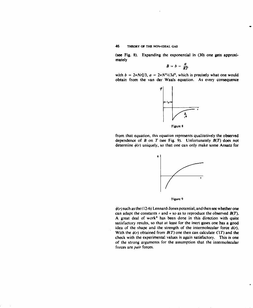
46 THEORY OF THE NON-IDEAL GAS
(see Fig. 8). Expanding the exponential in (30) one gets approxi-mately
B = b -- RT
with b = 2,Nro/3, a = 21,N 2A/3dI', which is precisely what one wouldobtain from the van der Waals equation. As every consequence
a-ro-.
Figure 8
from that equation, this equation represents qualitatively the observeddependence of B on T (see Fig. 9). Unfortunately B(T) does notdetermine 0(r) uniquely, so that one can only make some Ansatz for
T
Figure 9
,(r) such as the (12-6) Lennard-Jones potential, and then see whether onecan adapt the constants F and a so as to reproduce the observed B(T).A great deal of work8 has been done in this direction with quitesatisfactory results, so that at least for the inert gases one has a goodidea of the shape and the strength of the intermolecular force 0(r).With the 0(r) obtained from B(T) one then can calculate C(T) and thecheck with the experimental values is again satisfactory. This is oneof the strong arguments for the assumption that the intermolecularforces are pair forces.
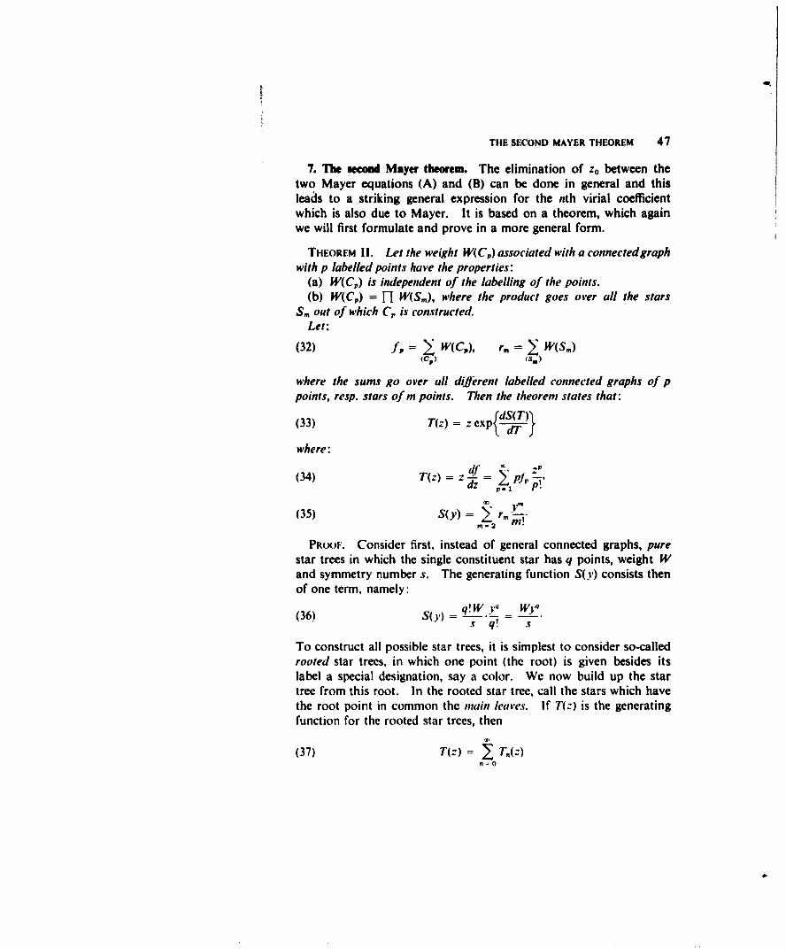
THE SECOND MAYER THEOREM 47
7. The second Mayer theorem. The elimination of z0 between thetwo Mayer equations (A) and (B) can be done in general and thisleads to a striking general expression for the nth virial coefficientwhich is also due to Mayer. It is based on a theorem, which againwe will first formulate and prove in a more general form.
THEOREM 11. Let the weight W(C,) associated with a connected graphwith p labelled points have the properties:
(a) W(C,) is independent of the labelling of the points.(b) W(C,) = 11 W(S.), where the product goes over all the stars
S. out of which Cr is constructed.Let:
(32) f, = > W(C,), r. = > W(S.)(Ce) fS3 )
where the sums go over all difterent labelled connected graphs of ppoints, resp. stars of m points. Then the theorem states that:
(33) T(z) = z exp{d,--•)}
where:
(34) T(:) = z ±f Pn
(35) S(y) = r
PROOF. Consider first, instead of general connected graphs, purestar trees in which the single constituent star has q points, weight Wand symmetry number s. The generating function S(y) consists thenof one term, namely:
(36) S(y) = i-W y, = Wy_s W. s
To construct all possible star trees, it is simplest to consider so-calledrooted star trees, in which one point (the root) is given besides itslabel a special designation, say a color. We now build up the startree from this root. In the rooted star tree, call the stars which havethe root point in common the main leaves. If T(:) is the generatingfunction for the rooted star trees, then
(37) T(:) = W T.(Z)n=O
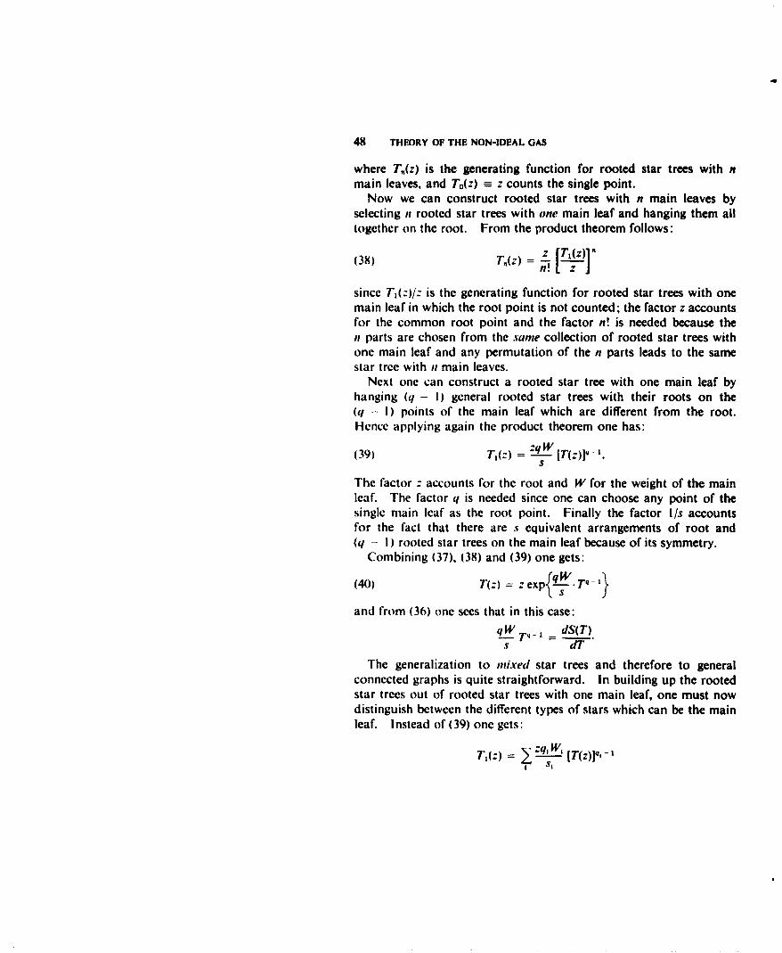
48 THEORY OF THE NON-IDEAL GAS
where T.(z) is the generating function for rooted star trees with nmain leaves, and To(z) z counts the single point.
Now we can construct rooted star trees with n main leaves byselecting n rooted star trees with one main leaf and hanging them alltogether on the root. From the product theorem follows:
(38) T .(z) = z
since Tl(:)/: is the generating function for rooted star trees with onemain leaf in which the root point is not counted; the factor z accountsfor the common root point and the factor n! is needed because thein parts are chosen from the same collection of rooted star trees withone main leaf and any permutation of the n parts leads to the samestar tree with it main leaves.
Next one can construct a rooted star tree with one main leaf byhanging (q - I) general rooted star trees with their roots on the(q - I) points of the main leaf which are different from the root.Hence applying again the product theorem one has:
(39) Tl(:) = _-W [T(:)Il_S
The factor : accounts for the root and W for the weight of the mainleaf. The factor q is needed since one can choose any point of thesingle main leaf as the root point. Finally the factor I/s accountsfor the fact that there are s equivalent arrangements of root and(q - I) rooted star trees on the main leaf because of its symmetry.
Combining (37), (38) and (39) one gets:
(40) T(-) = z exp-W. T-- ~S
and from (36) one sees that in this case:qW Tq_ dS(T)
S dT
The generalization to mixed star trees and therefore to generalconnected graphs is quite straightforward. In building up the rootedstar trees out of rooted star trees with one main leaf, one must nowdistinguish between the different types of stars which can be the mainleaf. Instead of (39) one gets:
T,(z) = [T(z)]q, -I1S,
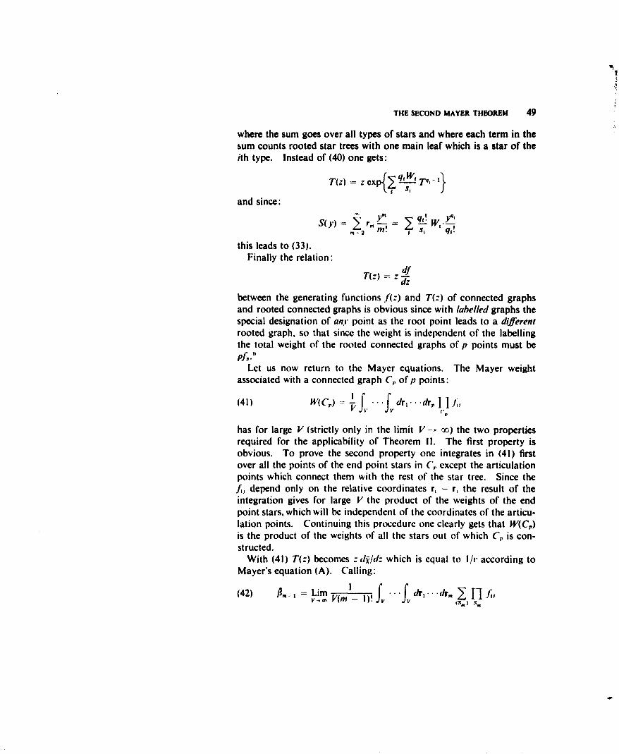
THE SECOND MAYER THEOREM 49
where the sum goes over all types of stars and where each term in thesum counts rooted star trees with one main leaf which is a star of theith type. Instead of (40) one gets:
T(z) z exp { -'W T1}
and since:s, - y , l f.l
m 2 M! fqi .this leads to (33).
Finally the relation:
T(z) = zdfZd
between the generating functions f(z) and T(z) of connected graphsand rooted connected graphs is obvious since with labelled graphs thespecial designation of any point as the root point leads to a differentrooted graph, so that since the weight is independent of the labellingthe total weight of the rooted connected graphs of p points must bePfH.9
Let us now return to the Mayer equations. The Mayer weightassociated with a connected graph C, of p points:
(41) ~W(CP) =j 1 /(41) f{ , p . . drý...U, I I,' (,p
has for large V (strictly only in the limit V - c) the two propertiesrequired for the applicability of Theorem If. The first property isobvious. To prove the second property one integrates in (41) firstover all the points of the end point stars in C, except the articulationpoints which connect them with the rest of the star tree. Since thef, depend only on the relative coordinates ri - r, the result of theintegration gives for large V the product of the weights of the endpoint stars, which will be independent of the coordinates of the articu-lation points. Continuing this procedure one clearly gets that W(Cp)is the product of the weights of all the stars out of which Cr is con-structed.
With (41) T(z) becomes z dkl/dz which is equal to 1 I/ according toMayer's equation (A). Calling:
(42) Bm-, Lim I fr .d. V(m - 1)f ... ,... (S,,) .:,
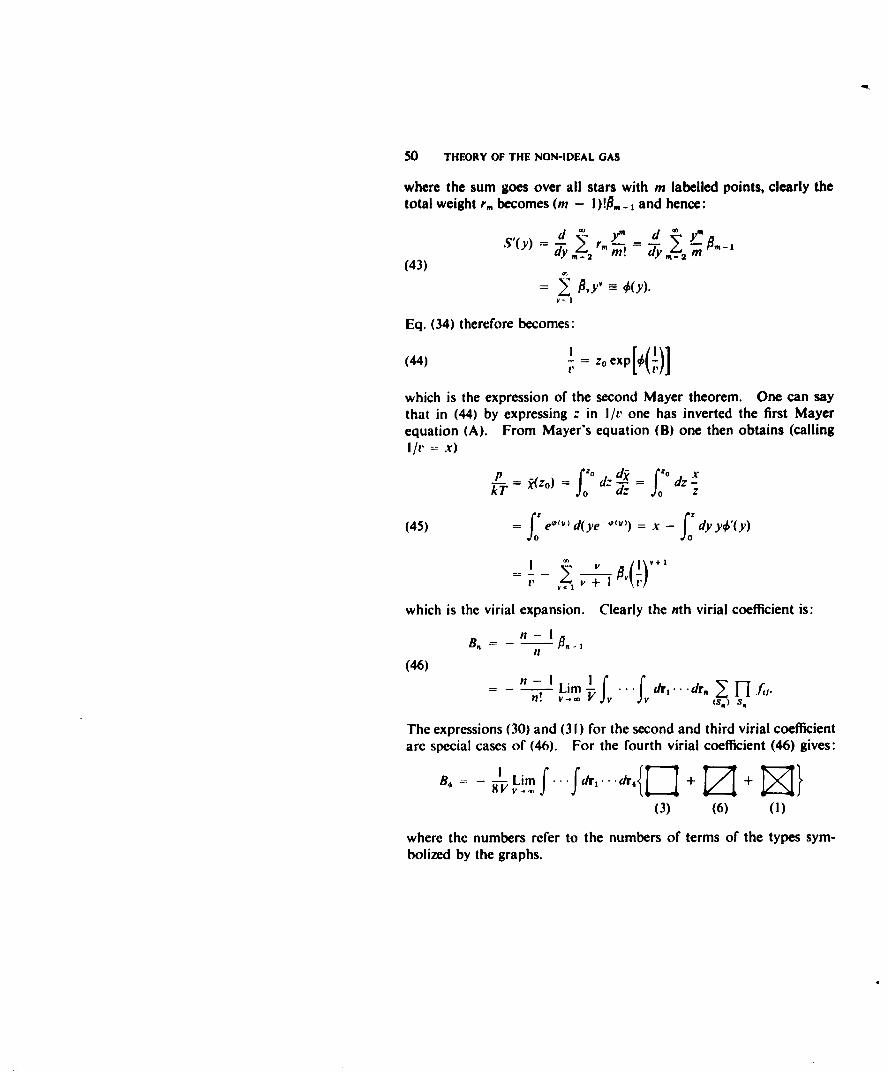
50 THEORY OF THE NON-IDEAL GAS
where the sum goes over all stars with m labelled points, clearly thetotal weight r. becomes (m - I)!#. 1 and hence:
S'(y) d . d m®
(43)
Eq. (34) therefore becomes:
H,(44) = zo exp[()
which is the expression of the second Mayer theorem. One can saythat in (44) by expressing z in I/v one has inverted the first Mayerequation (A). From Mayer's equation (B) one then obtains (callingI/v = x)
P = X Zo) =xdz d= -k-T z(O d X
(45) = fo e"' d(ye-p) = x - f: dy yOk(y)
- n IP1which is the virial expansion. Clearly the nth virial coefficient is:
(46) n ! Lim 1 . dr,1...dr I -R.f,.
n! V. Vf fý,(S,) S,~
The expressions (30) and (31) for the second and third virial coefficientare special cases of (46). For the fourth virial coefficient (46) gives:
B4 v- _ fm... fd . Er { V M
(3) (6) (I)
where the numbers refer to the numbers of terms of the types sym-bolized by the graphs.
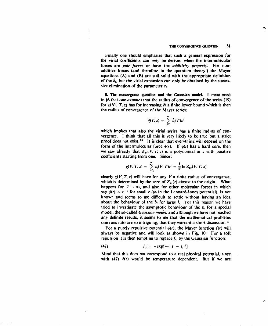
THE CONVERGENCE QUESTION 51
Finally one should emphasize that such a general expression forthe virial coefficients can only be derived when the intermolecularforces are pair forces or have the additivity properly. For non-additive forces (and therefore in the quantum theory!) the Mayerequations (A) and (B) are still valid with the appropriate definitionof the b,, but the virial expansion can only be obtained by the succes-sive elimination of the parameter zo.
8. The convergence question and the Gaussian model. I mentionedin §6 that one assumes that the radius of convergence of the series (19)for x(Nv, T, z) has for increasing N a finite lower bound which is thenthe radius of convergence of the Mayer series:
R(T, z) = . hb(T):1I~ 1
which implies that also the virial series has a finite radius of con-vergence. I think that all this is very likely to be true but a strictproof does not exist. 10 It is clear that everything will depend on theform of the intermolecular force 0(r). If 0(r) has a hard core, thenwe saw already that Zr( V, T, z) is a polynomial in z with positivecoefficients starting from one. Since:
X( V, T, Z) = bj( V, Tlz=- In Z( V, T, z)
clearly x( V, T, :) will have for any V a finite radius of convergence,which is determined by the zero of Zr(z) closest to the origin. Whathappens for V -- o, and also for other molecular forces in whichsay 0(r) r-" for small r (as in the Lennard-Jones potential), is notknown and seems to me difficult to settle without having an ideaabout the behaviour of the b, for large /. For this reason we havetried to investigate the asymptotic behaviour of the bh for a specialmodel, the so-called Gaussian model, and although we have not reachedany definite results, it seems to me that the mathematical problemsone runs into are so intriguing, that they warrant a short discussion."
For a purely repulsive potential 0(r), the Mayer function f(r) willalways be negative and will look as shown in Fig. 10. For a softrepulsion it is then tempting to replace f, by the Gaussian function:
(47) fj = -cxp[-.,r, - r,12].
Mind that this does not correspond to a real physical potential, sincewith (47) 0(r) would be temperature dependent. But if we are
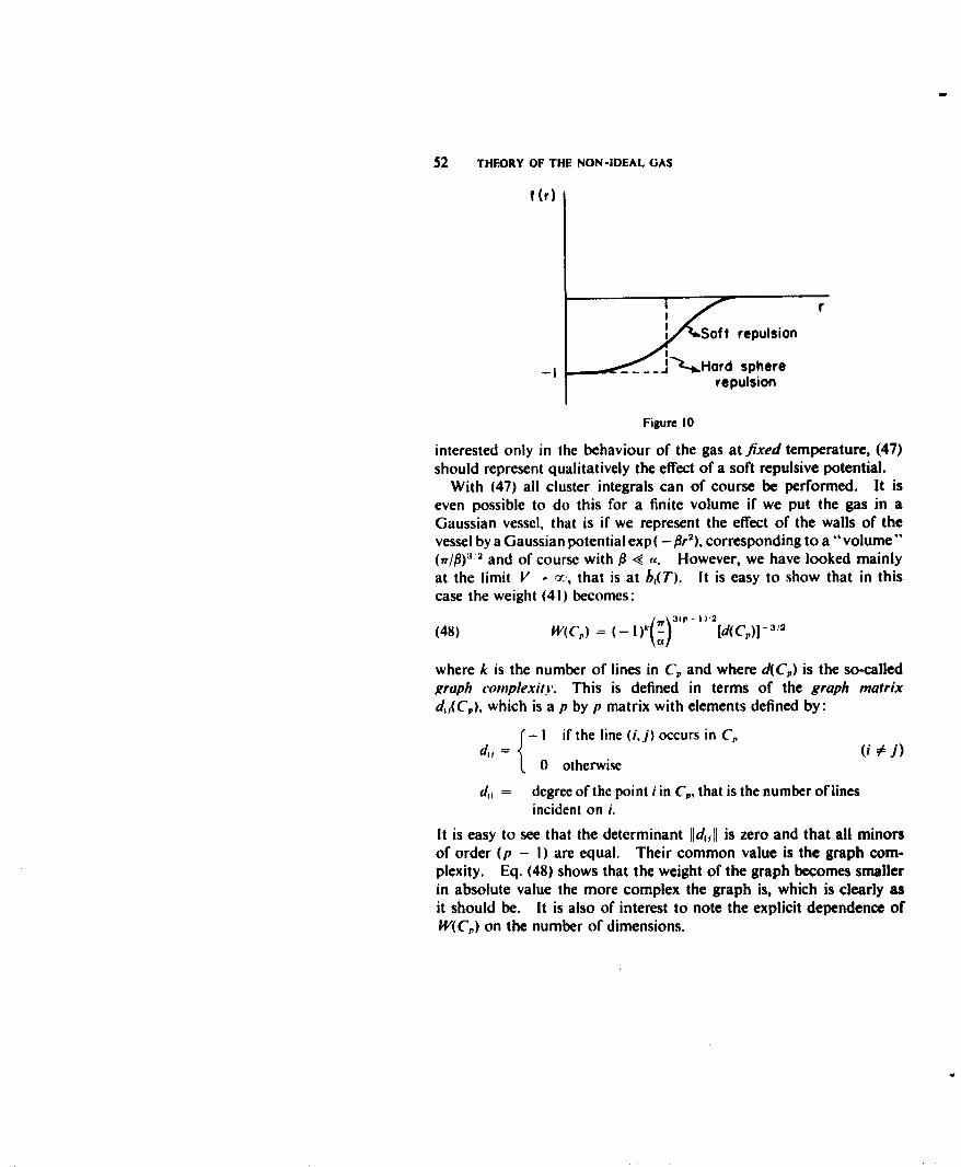
52 THEORY OF THE NON-IDEAL GAS
f (r)
r
Soft repulsion
-"�1-t-*.Hord sphererepulsion
Figure 10
interested only in the behaviour of the gas at fixed temperature, (47)should represent qualitatively the effect of a soft repulsive potential.
With (47) all cluster integrals can of course be performed. It iseven possible to do this for a finite volume if we put the gas in aGaussian vessel, that is if we represent the effect of the walls of thevessel by a Gaussian potential exp( - fr 2 ), corresponding to a "volume"(v/#i)3'2 and of course with f << a. However, we have looked mainlyat the limit V - ci:, that is at b1(T). It is easy to show that in thiscase the weight (41) becomes:(48) W(C) ( 2
3/2(45) w~c ) [d(c,)] ,
where k is the number of lines in C, and where d(C,) is the so-calledgraph complexitY. This is defined in terms of the graph matrixd,,(C), which is a p by p matrix with elements defined by:
- I if the line (ij) occurs in C,0 otherwise
d,= degree of the point i in Cp, that is the number of linesincident on i.
It is easy to see that the determinant 11d,11l is zero and that all minorsof order (p - I) are equal. Their common value is the graph com-plexity. Eq. (48) shows that the weight of the graph becomes smallerin absolute value the more complex the graph is, which is clearly asit should be. It is also of interest to note the explicit dependence ofW(C,) on the number of dimensions.
THE CONVERGENCE QUESTION 53
Many properties of graph matrices are known, but let me onlymention the following two theorems:1 2
(a) The graph complexity d(C€) is equal to the number of labelledCayley trees of p points which are subgraphs of C,.
(b) The sum of the complexities for all graphs Cpk of p labelledpoints and k lines is given by:
I(pI - 1)( - 2)(49) • d(C,) = p,- 2 -).
(Cpk) k- p + I
Clearly if we would know the distribution of the values of the graphcomplexity for all connected graphs of p points and k lines, thenone would be able to find an explicit expression for bp. In fact, ifn(p, k, d) is the number of graphs of p points, k lines and complexity d,then from (48) and the definition of b. it follows that:
P=(b"_I _LPIP J, k n(p, k, d)(50) I p - -) 3,2
kp-1 dI
where:
is the analogue of the van der Waals' b for this case (since b2 = -b)and where the sum over k goes over all the possible numbers of lineswhich can occur in a connected graph of p points. Of course, forfinite p and k only a discrete set of values of d is possible so thatn(p, k, d) is a step function, but if p increases and for k in the middleof its range actual numerical experience (all complexities for graphs upto p = 7 have been computed) 13 suggests that n(p, k, d) becomes agenuine smooth distribution function which in fact seems Gaussianaround its average value. It would be of great interest, I think, ifthese statements could be proved. Unfortunately at present all weknow about the distribution are the zeroth and first moments, since:
: n(p, k, d) = Clkd
where CPk, the number of connected (p, k) graphs can be found from(c), Note 7, and:
~~dn( ~~ (p -~)P~(( lXi' - 2V
d k -p + twhich is a rewriting of (49). We have been unable to compute highermoments. Already the second would be worth knowing!
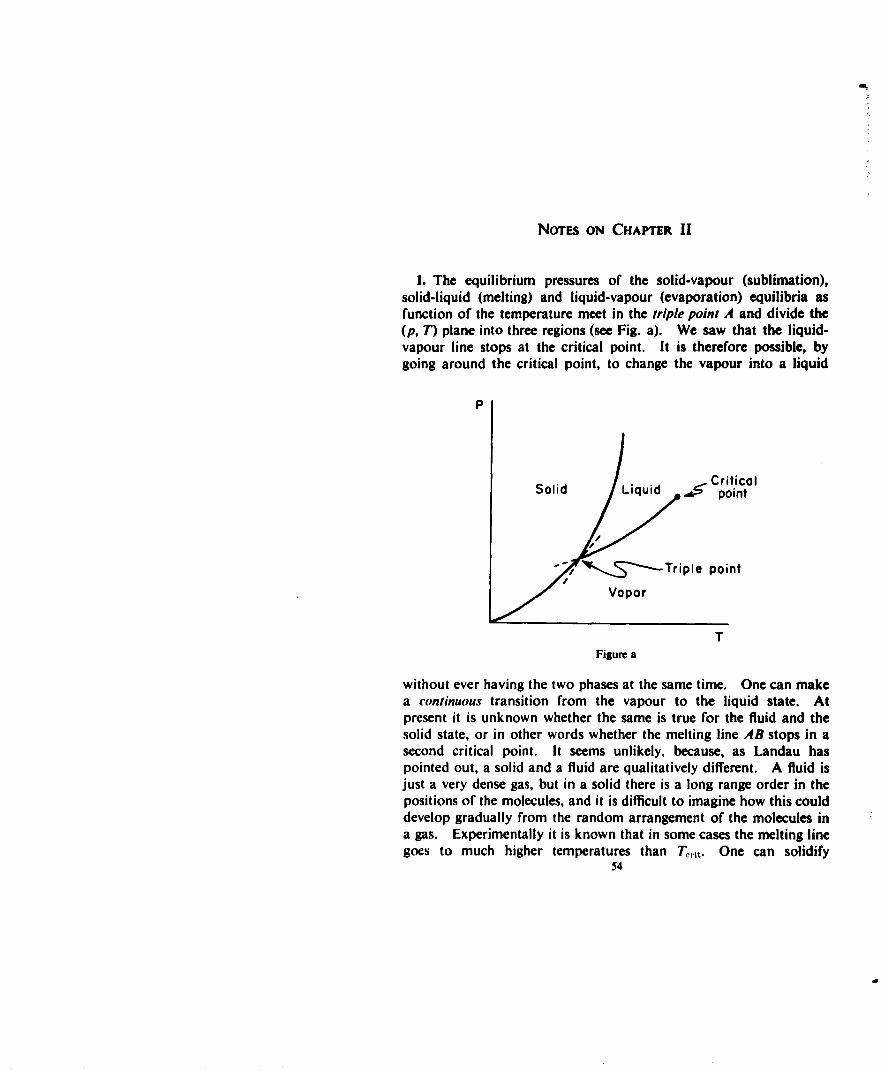
NOTEs ON CHAPTER II
I. The equilibrium pressures of the solid-vapour (sublimation),solid-liquid (melting) and liquid-vapour (evaporation) equilibria asfunction of the temperature meet in the triple point A and divide the(p, T) plane into three regions (see Fig. a). We saw that the liquid-vapour line stops at the critical point. It is therefore possible, bygoing around the critical point, to change the vapour into a liquid
P
CriticalSolid Liquid .& point
, %3-ýTripie point
Vapor
TFigure a
without ever having the two phases at the same time. One can makea continuous transition from the vapour to the liquid state. Atpresent it is unknown whether the same is true for the fluid and thesolid state, or in other words whether the melting line AB stops in asecond critical point. It seems unlikely, because, as Landau haspointed out, a solid and a fluid are qualitatively different. A fluid isjust a very dense gas, but in a solid there is a long range order in thepositions of the molecules, and it is difficult to imagine how this coulddevelop gradually from the random arrangement of the molecules ina gas. Experimentally it is known that in some cases the melting linegoes to much higher temperatures than Tent. One can solidify
54
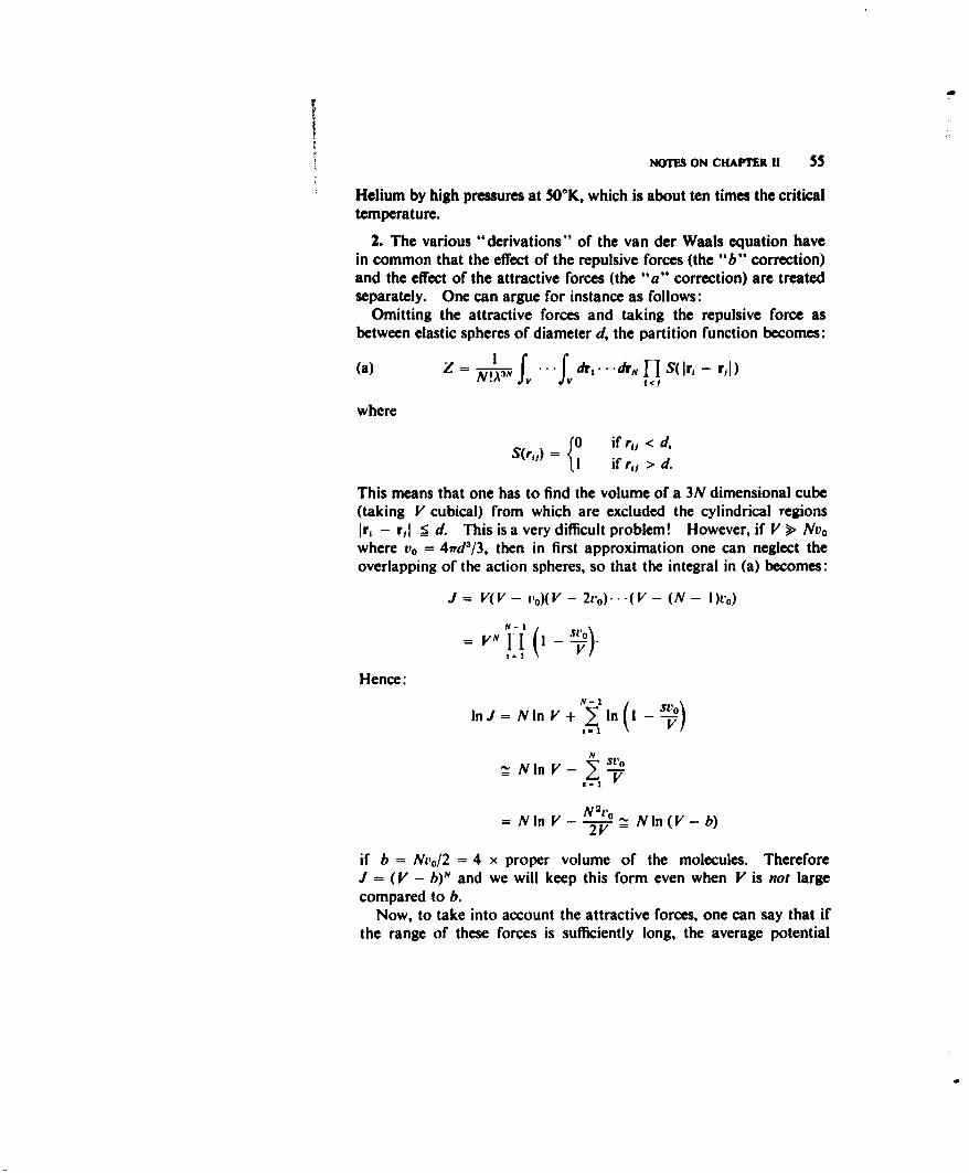
I
NOT7 ON CHAPTER 11 55
Helium by high pressures at 50*K, which is about ten times the criticaltemperature.
2. The various "derivations" of the van der Waals equation havein common that the effect of the repulsive forces (the "b" correction)and the effect of the attractive forces (the "a" correction) are treatedseparately. One can argue for instance as follows:
Omitting the attractive forces and taking the repulsive force asbetween elastic spheres of diameter d, the partition function becomes:
(a) z = I ... fdri. ..drN, S(Ir, - r11)
where
S(r,,)={0 if r, <d,I if r, > d.
This means that one has to find the volume of a 3N dimensional cube(taking V cubical) from which are excluded the cylindrical regionsIr, - rj, < d. This is a very difficult problem! However, if V >> Nvowhere vo = 4rd43/3, then in first approximation one can neglect theoverlapping of the action spheres, so that the integral in (a) becomes:
J = V(V - v0XV - 2'o)...(V - (N - I)v0)
= VN I-I(I - -,O)
Hence:
InJ= NIn V + ln V- )
N Nn V - --•
= NIn V - N2"V Nln(V - b)2V
if b = Nt'0/2 = 4 x proper volume of the molecules. ThereforeJ = (V - b)N and we will keep this form even when V is not largecompared to b.
Now, to take into account the attractive forces, one can say that ifthe range of these forces is sufficiently long, the average potential
56 THEORY OF THE NON-IDEAL GAS
energy will be - CN2/2 V, since each molecule attracts all moleculesin its action sphere and the number of these molecules will be pro-portional to the number density NIV. C is a positive constant andthe contribution to the partition function is therefore roughlyexp( +a/VkT) with a = CN2/2. Altogether one gets therefore:
(b) Z = 1 el/Vkr(V - b)NN !A3 N
and from p = kTb(ln Z)/1 V van der Waals equation follows.
3. This was first pointed out by J. de Boer (Dissertation, Amster-dam, 1940; Physica 14 (1948) 139). It is important to note that themass of the molecule does not affect the equation of state in theclassical theory to which we restrict ourselves. In the quantumtheory this is no longer true. The equation of state, using the sameintermolecular potential, then depends on a third dimensionlessvariable, the so-called de Boer parameter:
hA=(me) 2
See also the dissertation of R. J. Lunbeck (Amsterdam, 1951).
4. H. D. Ursell, Proc. Cambridge Philos. Soc. 23 (1927) 685. Thework of Mayer is summarized in the book of J. E. Mayer and M. G.Mayer, Statistical Mechanics (Wiley, New York, 1940). For thegeneralization to the quantum theory see B. Kahn and G. E. Uhlen-beck, Physica 5 (1938) 399; B. Kahn (Dissertation, Utrecht, 1938).For the generalization to the Bose or Fermi statistics see T. D. Leeand C. N. Yang, Phys. Rev. 113(1959) 1165.
5. Most of the terminology is the same as in the book of Kdnig(Theorie der Endlichen und Unendlichen Graphen, Leipzig, 1936).There is no special term for a graph without articulation points, andit is convenient to have one. The word star and the correspondingnotion of star tree were introduced in our paper on the combinatorialproblems in the theory of graphs (Proc. Nat. Acad. Sci. U.S.A. 42(1956) 122).
6. The following presentation of the Mayer theory follows a reviewarticle by G. W. Ford and G. E. Uhlenbeck entitled: The theory oflinear graphs with applications to the theory of the virial developmentof the properties of gases, which appears in Studies in statistical
NOTES ON CHAPTER 11 57
mechanics Vol. I (North Holland Publishing Company, Amsterdam,1962).
7. If one takes in Theorem I for the weight W, yk, where y is anarbitrary variable and k is the number of lines in the graph G, or C1,then it is clear that W fulfills all the requirements, and that thereforeTheorem I is applicable. One obtains:
(W) I + N(x, y) = ••.11
where: 00Xp •P-- 1)/2
(d) N(x,y) = . .Nky,.P k-
(e) C(x, y) =0x ( ~ -, U1 )
and:
NPk= number of labelled (p, k) graphs (= graphs of ppoints and k lines)
(f) = (Ip(P k )/2),
C'k = number of connected, labelled (p, k) graphs.
Eq. (c) was first derived by R. J. Riddell (Dissertation, University ofMichigan, 1951). It allows the calculation of the numbers Cpk interms of the known binomial coefficients Npk.
8. For a complete account see the book by J. 0. Hirschfelder,C. F. Curtiss and R. B. Bird, The Molecular Theory of Gases andLiquids (Wiley, New York, 1954). A very useful summary of thetheoretical calculations of the virial coefficients is given by T. Kihara,Revs. Modern Phys. 25 (1953) 831; 27 (1955) 412.
9. By taking as in Note 7 for the weight W, yk (k = number oflines in the graph) one sees that the two requirements for the weightW(Cp) are fulfilled so that Theorem 11 is applicable. Writing:
(g) S(x, y) = S! y
p-2
k-p-I
where Sk is the number of stars with p labelled points and k lines(with the convention S21 = I), and putting:
z(x, y) = x x C(x, y)
58 THEORY OF riHe NON-IDEAL GAS
where C(x, y) is giY c1i, (c), then Theorem II yields the second Riddellformula:
(h) -S(z,y) = InZ.(h) x
From (h) one can find S,,, in terms of the C,,. It is not difficult toshow that for large p and k > p In p the numbers Npk, C,, and S~kare asymptotically equal, so that one can say that for large p andk > p In p the overwhelming majority of the graphs are stars.
10. For a time the convergence question seemed (even to thephysicist!) of great interest because Mayer, Kahn and Uhlenbeck (seeNote 4 for the literature) had speculated and had tried to prove thatthe nearest singularity of R(T, z) on the positive real z-axis (assumingthat there R and d•/dz remain finite) would determine the point ofcondensation of the gas. This was strongly suggested by the case ofthe ideal Bose gas, which is of course not a special case of the non-ideal gas theory we have discussed (since the deviations of the idealgas laws are in this case due to quantum effects), but which is a casefor which the corresponding b, can be evaluated explicitly. In fact,already in 1925 Einstein derived for the Bose gas the equations:
I I M ,At
I=!
0)
p -1 .A'1.1
which have precisely the same form as the Mayer equations if oneputs:
A A30-T1Z X3 b,(T) = -_75-.
Clearly the series:
g(A) =
is convergent up to A = I, which is the nearest singularity on thepositive real axis of the analytic function generated by the series. Thepoint A = I is a branchpoint of order two and R and dR/dA are finiteat this point. It is known, and it can be proved in various ways, that
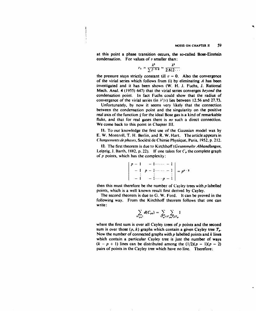
NOTES ON CHAPTER II 59
at this point a phase transition occurs, the so-called Bose-Einsteincondensation. For values of v smaller than:
A3 A3
Y1' = ) = 2.612...the pressure stays strictly constant till v = 0. Also the convergenceof the virial series which follows from (i) by eliminating A has beeninvestigated and it has been shown (W. H. J. Fuchs, J. RationalMech. Anal. 4 (1955) 647) that the virial series converges beyond thecondensation point. In fact Fuchs could show that the radius ofconvergence of the virial series (in A3/v) lies between 12.56 and 27.73.
Unfortunately, by now it seems very likely that the connectionbetween the condensation point and the singularity on the positivereal axis of the function g for the ideal Bose gas is a kind of remarkablefluke, and that for real gases there is no such a direct connection.We come back to this point in Chapter Ill.
11. To our knowledge the first use of the Gaussian model was byE. W. Montroll, T. H. Berlin, and R. W. Hart. The article appears inChangementsdephases. Soci6ti de Chimie Physique, Paris, 1952, p. 212.
12. The first theorem is due to Kirchhoff (Gesammelte Abhandlungen,Leipzig, J. Barth, 1882, p. 22). If one takes for C, the complete graphof p points, which has the complexity:
p- I - I .....- I-I p-I ...- I =p- 2
-I -i.... p-
then this must therefore be the number of Cayley trees with p labelledpoints, which is a well known result first derived by Cayley.
The second theorem is due to G. W. Ford. It can be proved in thefollowing way. From the Kirchhoff theorem follows that one canwrite:
(Cp•) (r,) (c,,):) Ta,
where the first sum is over all Cayley trees of p points and the secondsum is over those (p, k) graphs which contain a given Cayley tree T,.Now the number of connected graphs with p labelled points and k lineswhich contain a particular Cayley tree is just the number of ways(k - p + I) lines can be distributed among the (1/2)(p - l)(p - 2)pairs of points in the Cayley tree which have no line. Therefore:
60 THEORY OF THE NON-IDEAL GAS
=i (P: -10 2))(c,• , k - p +!
and since there are p" -2 Cayley trees with p points, Eq. (49) follows.
13. For tables see the article referred to in Note 6. Note, that onecan formulate the problem of finding the distribution function n(p, k, d)also in the following way. Find the distribution of the first principalminor of random, symmetric p by p matrices in which with equal apriori probability k of the p(p - 1)/2 off-diagonal elements, say onthe right of the main diagonal, are set equal to minus one and the restequal to zero. The matrix is then completed by taking each diagonalelement equal to the sum of the elements on the corresponding row(or column) with the opposite sign.
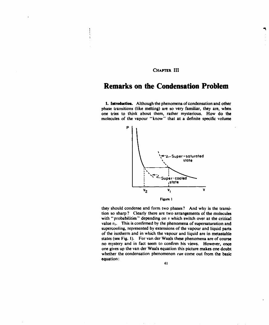
CHAPTER III
Remarks on the Condensation Problem
1. latrodutiom. Although the phenomena of condensation and otherphase transitions (like melting) are so very familiar, they are, whenone tries to think about them, rather mysterious. How do themolecules of the vapour "know" that at a definite specific volume
P
?-.--Super -saturated% state
sstateI I
V2 V1 V
Figure I
they should condense and form two phases? And why is the transi-tion so sharp? Clearly there are two arrangements of the moleculeswith "probabilities" depending on v which switch over at the criticalvalue vj. This is confirmed by the phenomena of supersaturation andsupercooling, represented by extensions of the vapour and liquid partsof the isotherm and in which the vapour and liquid are in metastablestates (see Fig. I). For van der Waals these phenomena are of courseno mystery and in fact seem to confirm his views. However, onceone gives up the van der Waals equation this picture makes one doubtwhether the condensation phenomenon can come out from the basicequation:
61
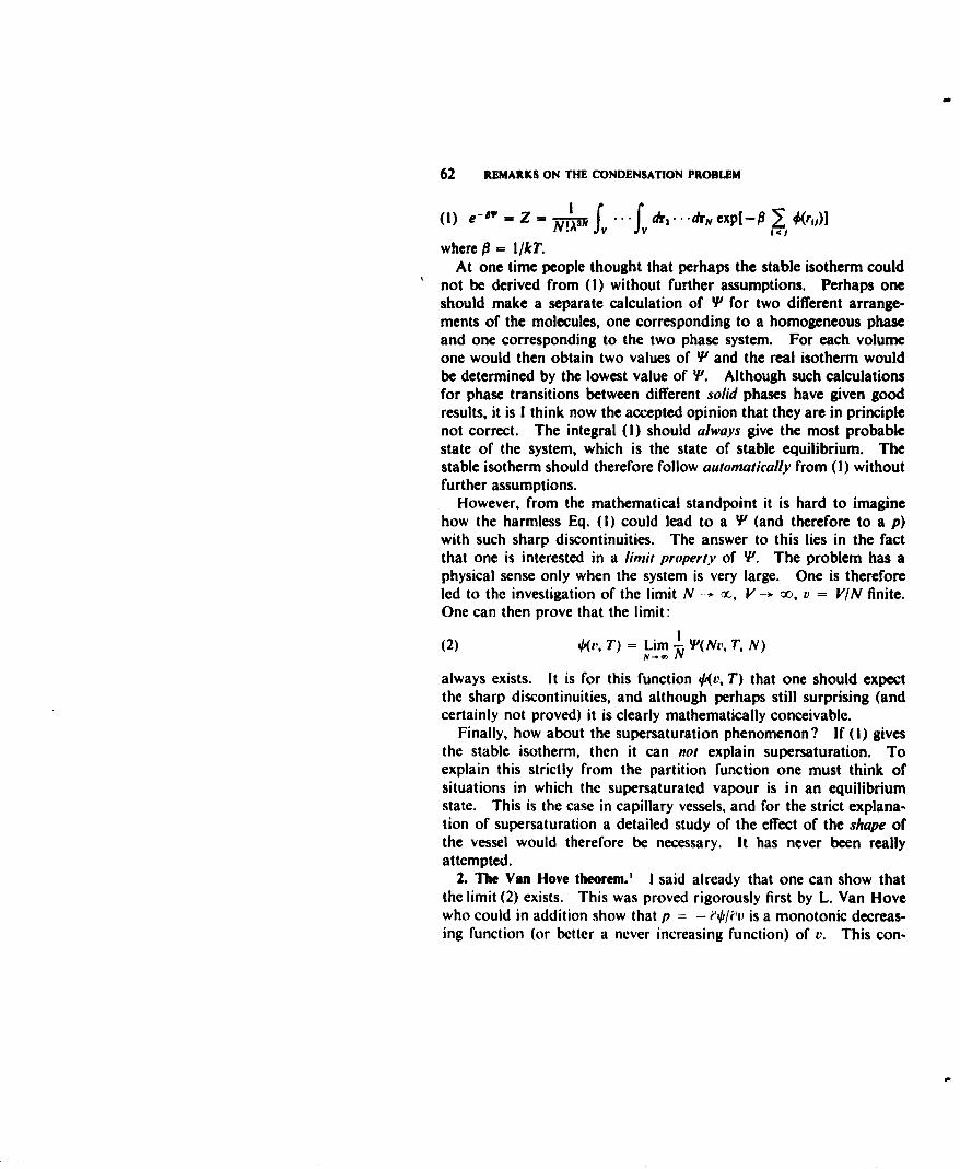
62 REMARKS ON THE CONDENSATION PROBLEM
(I) e-.," = Z = I . dr, ... dr,, exp[-0Fi)
where P = l/kT.At one time people thought that perhaps the stable isotherm could
not be derived from (I) without further assumptions. Perhaps oneshould make a separate calculation of YJ for two different arrange-ments of the molecules, one corresponding to a homogeneous phaseand one corresponding to the two phase system. For each volumeone would then obtain two values of W and the real isotherm wouldbe determined by the lowest value of V. Although such calculationsfor phase transitions between different solid phases have given goodresults, it is I think now the accepted opinion that they are in principlenot correct. The integral (I) should always give the most probablestate of the system, which is the state of stable equilibrium. Thestable isotherm should therefore follow automatically from (I) withoutfurther assumptions.
However, from the mathematical standpoint it is hard to imaginehow the harmless Eq. (I) could lead to a T (and therefore to a p)with such sharp discontinuities. The answer to this lies in the factthat one is interested in a limit property of W. The problem has aphysical sense only when the system is very large. One is thereforeled to the investigation of the limit N -- a, V --* a, v = V/N finite.One can then prove that the limit:
(2) Or, T) = Lim - l(N', T, N)N-.~ N
always exists. It is for this function O4v, T) that one should expectthe sharp discontinuities, and although perhaps still surprising (andcertainly not proved) it is clearly mathematically conceivable.
Finally, how about the supersaturation phenomenon? If (i) givesthe stable isotherm, then it can not explain supersaturation. Toexplain this strictly from the partition function one must think ofsituations in which the supersaturated vapour is in an equilibriumstate. This is the case in capillary vessels, and for the strict explana-tion of supersaturation a detailed study of the effect of the shape ofthe vessel would therefore be necessary. It has never been reallyattempted.
2. The Van Hove theorem.' I said already that one can show thatthe limit (2) exists. This was proved rigorously first by L. Van Hovewho could in addition show that p = - i¢/b' is a monotonic decreas-ing function (or better a never increasing function) of v. This con-
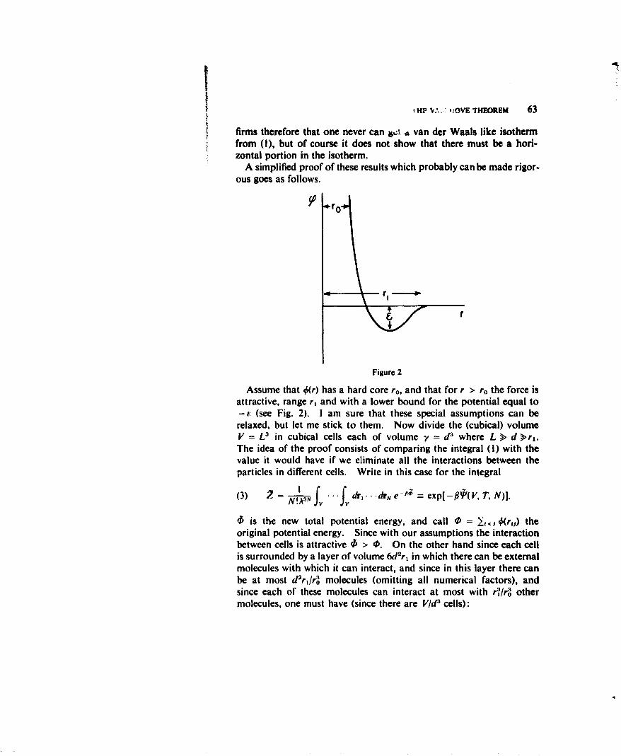
SHP *VA O ;OVE THEOREM 63
firms therefore that one never can jt % van der Waals like isothermfrom (1), but of course it does not show that there must be a hori-zontal portion in the isotherm.
A simplified proof of these results which probably can be made rigor-ous goes as follows.
5 ,ro!
Figure 2
Assume that 0(r) has a hard core ro, and that for r > ro the force isattractive, range ri and with a lower bound for the potential equal to-,. (see Fig. 2). I am sure that these special assumptions can berelaxed, but let me stick to them. Now divide the (cubical) volumeV = -L in cubical cells each of volume y = d' where L > d >r1 .The idea of the proof consists of comparing the integral (I) with thevalue it would have if we eliminate all the interactions between theparticles in different cells. Write in this case for the integral
(3) 2 = fv'"fdr.. "drNe-" = exp[-#P(V, T, N)].
'5 is the new total potential energy, and call 0 = 4, #(rj) theoriginal potential energy. Since with our assumptions the interactionbetween cells is attractive 40 > 0. On the other hand since each cellis surrounded by a layer of volume 6d2r, in which there can be externalmolecules with which it can interact, and since in this layer there canbe at most d2r,/r• molecules (omitting all numerical factors), andsince each of these molecules can interact at most with r'frg othermolecules, one must have (since there are V/d 3 cells):
64 REMARKS ON THE CONDENSATION PROBLEM
d 2r1 rl V
ro3 r~od3
Hence one can conclude:e- _<- e-10 < exp[-# + p#V/dJ
with p = r4/04. The integration over r.. r,, does not change thedirection of the inequalities and by calculating the free energies Wand W one obtains:
(4) q % fj + f PN =N =N d
where v = V/N. Since increasing N, keeping v fixed, one still can
let d -, o say as N" ', one sees that WIN and WIN will approach tothe same limit if such a limit exists. Now
I S , !n!N!" f r!3 F • .. ,. dr,. •dr., exp[ - #0 r,... r.)]
(5) N ,, ln !. .n!Y
- S exp[-f 2 n.0.,(,. y))(Ini) t: 1
where the sum is over all numbers n, of particles in the ith cell, withthe condition (indicated by the prime):
n, = N,
and where we have put:
(6) e8 #",*(fv) = ' f .f dr1 .. dr,, exp[- #0(r, )
Many of the numbers n, may still be equal to each other. Let ak bethe number of cells in which the number of molecules is k, then(7) 2-= Sxp[e-p9-1 kakO(k, y)]
(all) k
where the double prime indicates the conditions:
(8) =ak ka = N.k k
Calling:
ok s e-ok*(kie)
one sees that (7) is of the multinomial form and one knows that for Y
THE VAN HOVE THEOREM 65
and N large it is closely approximated by the maximum term in thesum, for which:
(9) ak - Agkzk
where A and z must be determined from (8). In fact:
(10) In2! -NInz +- vin(z)
with:a(z) - , >gz.
k
From (8) and (9):do
v = Ao(z), N = Azdz
so that since v = V/d 3 = Nr/d3, one has:
(II) d1 a
For fixed d, z depends therefore only on r and from (9) it then follows(always for fixed d) that:
(12) In2, - In: + -lna(z) = r).
Together with the inequality (4), this shows that the limit (2) exists.Furthermore from the inequality (4) it follows that also p = - 0&vand f = iý,/0, differ at most by a constant quantity proportional toI/d, and which can therefore be made as small as one wishes. Soit is sufficient to look at P. From (12) follows:
I In a(z),
(13)= I d In a(z) dz
For #d 3 dz dv
and from (II) one gets:
dA d" [32 do\ 2 -2 d )d
d: zdu/dZ)2 [Z (a) d_ (xZ()]
(14) z3(do/IdZ)2 [R kg?)-( gkzj k~gz)
d3 -.dz (k- j) 2ggzk + I < 0.2z3(do/dz)2k1
66 REMARKS ON THE CONDENSATION PROBLEM
Since all g, > 0, one sees from (I 3 that the sign of ap/8v is determinedby dz/dv, and from (14) one can then conclude that O.f/8v and thereforeOp/8v < 0, which is the content of the second part of the Van Hovetheorem.2
3. The ideas of Yang and Lee. In a very interesting paper3 Yang andLee have shown a way how the condensation phenomenon couldfollow mathematically from the basic equation (1) in the limitN, V - o, I, = V/N fixed. Their starting point is the grand canonicalpartition function:
Zgr(V, T,:) = • (A3z)NZ(V, T, N)N-O
for which we derived in Chapter lf the expression:
(15) Zgr(V, 7", T) = exp{ Vx(V, T. z)}
which is valid for any finite V. With the assumption of a hard core,radius r., we already noted that Z, must be a polynomial of degreeM 2 V/rgo. Let the zeros of this polynomial be z, then (droppingfrom now on the T, which remains constant anyway):
(16) Z.,(V, Z) = f -)
and
(17) x(V.: =j-Zll -I•
1=1 Zj
One can therefore interpret x( V, :) as the complex logarithmic potentialof M point charges of strength I/V situated at the points z. Notethat since the coefficients of the polynomial Zg.( V,z) are positive,none of the zeros :, can be on the positive real axis, so that x(V, z),for fixed V, will be an analytic function of z along the positive realaxis.
Let us now look at the limit V - . For increasing V the strengthof the charges become smaller and smaller, while the number Mincreases. Suppose now that in the limit V- oo a number of thepoint charges concentrate themselves in a single layer AB which crossesthe positive real axis. Of course in addition there may be other layerslike CD and finite poles P1. P2,.. (see Fig. 3). The function:
(18) g(z) = Limx(V, :)
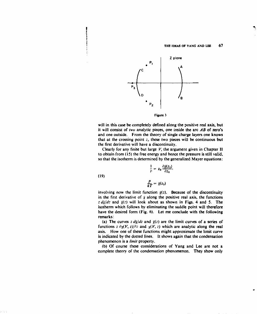
THE IDEAS OF YANG AND LEE 67
Z ploneP1 • A
C
P3
D )
P2
Figure 3
will in this case be completely defined along the positive real axis, butit will consist of two analytic pieces, one inside the arc AB of zero'sand one outside. From the theory of single charge layers one knowsthat at the crossing point :, these two pieces will be continuous butthe first derivative will have a discontinuity.
Clearly for any finite but large V, the argument given in Chapter I1to obtain from (15) the free energy and hence the pressure is still valid,so that the isotherm is determined by the generalized Mayer equations:
I = zo
(19)P- = V~Z0)
involving now the limit function Z(Z). Because of the discontinuityin the first derivative of g along the positive real axis, the functionsz dgl/d: and g(:) will look about as shown in Figs. 4 and 5. Theisotherm which follows by eliminating the saddle point will thereforehave the desired form (Fig. 6). Let me conclude with the followingremarks:
(a) The curves : dg/dz and j(:) are the limit curves of a series offunctions : Ox(V, z)/?: and x( V, :) which are analytic along the realaxis. How one of these functions might approximate the limit curveis indicated by the dotted lines. It shows again that the condensationphenomenon is a limit property.
(b) Of course these considerations of Yang and Lee are not acomplete theory of the condensation phenomenon. They show only
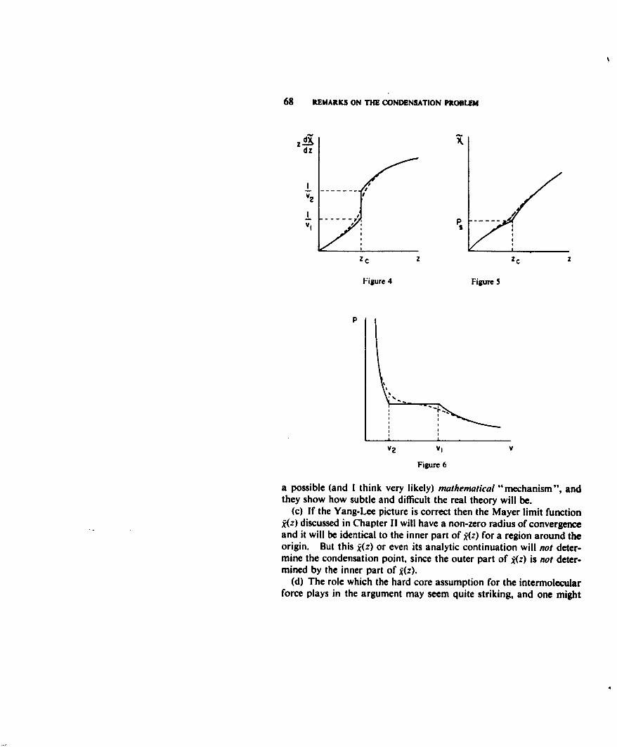
68 REMARKS ON THE CONDENSATION PROBLEM,dz
Vt-- SP----
Z C Z ZC
Figure 4 Figure 5
P
V2 V1 V
Figure 6
a possible (and I think very likely) mathematical "mechanism", andthey show how subtle and difficult the real theory will be.
(c) If the Yang-Lee picture is correct then the Mayer limit functionR(z) discussed in Chapter ii will have a non-zero radius of convergenceand it will be identical to the inner part of g(z) for a region around theorigin. But this R(z) or even its analytic continuation will not deter-mine the condensation point, since the outer part of g(z) is not deter-mined by the inner part of g(z).
(d) The role which the hard core assumption for the intermolecularforce plays in the argument may seem quite striking, and one might
SOME EXAMPLS 69
even think that therefore a gas of hard spheres will also show thecondensation phenomenon. This is of course not necessarily so.The charges may concentrate in single layers, but if for V--> 0 thecharges do not close down on the real axis, that is to say if there isalways a gap, then there will be no condensation since g(z) will thenbe analytic along the whole real axis.
4. Some exampll s. 4 To make things more concrete, we considerhere a few artificial examples constructed to illustrate the analyticfeatures of the theory. Unfortunately, no one has ever been able tocompute the partition function for a realistic model of a gas, so ourexamples must be quite ad hoc.
Suppose that the grand canonical ensemble partition function hasthe form:
(20) Zgr(V, Z) = (0 + z)v I -
where we take Vto be an integer. Here Vis, say, the volume measuredin units ro4 and is analogous to the M in Eq. (16). The canonicalensemble partition function corresponding to (20) is obtained byexpanding in powers of : and identifying A( V, N) as the coefficient of:N. We find:
(21) Z(VN)= N.(N -No)0:E(NO -0 N)
This model has been constructed so that it has the general featureswhich the partition function of a real gas must have, i.e. the functionZr( V, z) is a polynomial of degree 2 V with positive coefficients andthe coefficients are monotonically increasing functions of V for fixedN. In our example (20) the 2 V zeros of Zr are all on the unit circle,half of them at z = - 1, the other half at the Vth roots of unity otherthan z = - I. There are no real positive zeros. It is now easy toshow that for this model the limit function g(z) is given by:
(22) In ( + z), forz< 1,In (I + z) + Inz, forz > 1.
This is just the logarithmic potential due to one unit of charge atz = - I and one unit of charge distributed in a uniform single layeron the unit circle. The function R(z) is continuous along the positivereal axis but its derivative has a discontinuity at z = I. Note thatg(z) outside the unit circle is not the analytic continuation of g(z)
70 REMARKS ON THE CONDENSATION PROBLEM
inside the circle. Also note that the function g(z) introduced in §6,Ch. 11 is just:
(23) g(z) = In (I + z).
This function has no singularities along the positive real axis, indeedits only singularities are logarithmic branchpoints at z = -1 andZ= 0-.
The equation of state corresponding to (22) is readily obtainedusing the Mayer equations (19). We find
I v I I In 1 _ ! = +T - 5 +- + ., v> 2,
(24) kTP = iIn 2 ,2 > v > ,
{n( 2v 1)2 ' T
This is the typical form of the isotherm for a condensing gas. Notethat the virial expansion of the equation of state is convergent forv > I while the gas condenses at tv = 2. Hence, an important thingwe learn from this model is that we cannot in general determine thepoint of condensation or the properties of the condensed phase froma study of the equation of state in the gas phase alone, i.e. from thevirial series.
Note that one can obtain the equation of state also directl/ bycomputing the limit:
I r) = Lim I/InZ(Nt,, N)
using (21) for Z(V, N). One does not need to introduce the grandcanonical partition function, although of course it is quite a goodtrick!
It may still be of interest to consider a wider class of models, namelythose in which the zeros of Z,, all lie on the unit circle. If we intro-duce g(g) such that Vg(O) dO is the number of zeros of Zgr which liebetween 0 and 0 + dO on the unit circle, then the limit function &(:)will be the logarithmic potential due to a charge distribution withdensity g(#) on the unit circle, so that:
(25) *lz) = dOg(O) In (I - ze'°).
Since Zgr is a real function its zeros must be distributed symmetricallywith respect to the real axis, i.e.
Ii
SOME EXAMPLES 71
(26) g(a) - A 0),
We can find further properties of g(O) by expanding both sides of (25)in powers of z for Izl < I. Since for jzj < 1:
(27) V(z) =(z) ()= ,l- I
one finds:
(28) b -= f A d g(O) cosIO.
Thus, the b,'s are directly related to the coefficients in the Fouriercosine series expansion of g(0). Hence we can write:
I I W b o 0
(29) g(O) = y -- :E .
Here,
(30) go = 0 " dO g(O)
is the total charge in the distribution. From (29) we see explicitlythat g(0) cannot be completely determined from a knowledge of theb,'s, i.e. from g(z); there is still the undetermined constant go. From(25) one can readily show that in general:
(31) X(z) = X() + go In z.(31))
Hence, we can write
W(), Iz < I,(32) R(z)= + golnz, jzj > !.
Here we see explicitly that g in the outer region cannot in general bedetermined from g in the inner region.
NOTES ON CHAPTER III
1. L. Van Hove, Physica 15 (1949) 95 1. We follow the presentationgiven by R. J. Riddell in his dissertation (Contributions to the Theoryof Condensation, University of Michigan, 1951).
2. This proof should be compared with the proof given by C. N.Yang and T. D. Lee, Phys. Rev. 87 (1952) 404, Appendix I. Withthe same assumptions for the intermolecular potential and usingessentially the same method as Van Hove, Yang and Lee prove thatthe limit:
(a) g(T, :) = Lim- In Zg(V, T, z)V-M
exists. In addition they prove that both g(:) and z 0/z for positivereal z are monotonically increasing with increasing z and that Xz)must be continuous.
Since the grand partition function Z.r is a polynomial with positivecoefficients from which for large N the partition function Z(Nv, T, N)follows by the steepest descent method (see Chapter 1i, §7) it is clearthat from the existence of the limit (a) and from the properties of gand z ilgliz both parts of the Van Hove theorem follow. The questionarises whether the inverse of this statement is also true. Can onededuce from the Van Hove theorem the existence of the limit (a) andthe properties of 9(z). This is of course very likely but a formalproof (which we owe to M. Kac) is perhaps not superfluous.
Let us assume that with increasing volume the vessel always keepsthe same shape. One then can introduce a Laplace transform ofZur by:
fbfdVe-'vZr(V",Tz)= I ZN f dVe- vZ(V, T, N)(b) f N-0O
= + NzN dv e N-I'Z(N,, N)
putting V = Ni, and omitting from now on the variable T. Since forfixed N, Z(Nv, N) - v for large v, (ideal gas limit) the integral in (b)for s > 0 always converges, and one can conclude that the abscissa ofconvergence of the Laplace integral is determined by the convergence
72
NOTES ON CHAPTER 111 73
of the series over N. According to the first part of the Van Hovetheorem Z(Nv, N) ! exp( - Npov)) if N is large. Using the methodof steepest descent the integral in (b) can therefore for large N beapproximated by:
(c) dve_ ,.+o#(,ll 12f e- N- vo +(200))1= \No"(Vo)!
where the saddle point vo is determined by
(d) s + , =)=0."bV0
Here we also have used the fact that for v > 0 00l/v < 0 and " -0
2,/Ov 2 > 0 which follows from the second part of the Van Hovetheorem and from the fact that the pressure p = -00/fv is alwayspositive, since it is positive in the ideal gas limit.
From (b) and (c) one concludes that the abscissa of convergenceof the Laplace integral is that positive value of s - for which:
(e) ze - 1;,'o + 5*(V")) = I
where vo is determined from (d) which we now write as:
(f) 9= -9ePI)
h.'0
Eqs. (e) and (f) are two simultaneous equations from which g and v0are to be determined as functions of z. We shall show from theVan Hove theorem that there is always an unique solution for g, whichimplies that for large V:
Zr( V, z) z ev;(Z)
so that the Yang-Lee limit (a) exists. The properties of X(z) alsofollow from (e) and (f). To see all this, write Eq. (e) in the form:
(g) 00vo) - 1 o = I In) z
using (f). This is now an equation for vo as function of z, and then (f)determines g. Eq. (g) can most easily be discussed graphically.Suppose first that no condensation occurs. Then according to VanHove 4#(v) is a monotonic decreasing and upward concave functionof v. For any value of z, v. is then uniquely determined by drawing
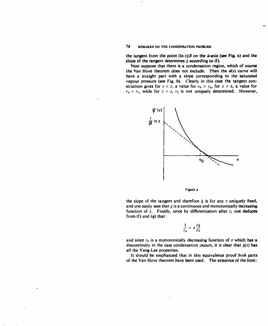
74 REMARKS ON THE CONDENSATION PROBLEM
the tangent from the point (In z)/l on the 0-axis (see Fig. a) and theslope of the tangent determines g according to (f).
Next suppose that there is a condensation region, which of coursethe Van Hove theorem does not exclude. Then the 0(v) curve willhave a straight part with a slope corresponding to the saturatedvapour pressure (see Fig. b). Clearly in this case the tangent con-struction gives for z < z, a value for vo > V., for z > z, a value forVo < V,, while for z= z, v0 is not uniquely determined. However,
Wi)v)
SInZ
Figure a
the slope of the tangent and therefore g is for any z uniquely fixed,and one easily sees that R is a continuous and monotonically increasingfunction of z. Finally, since by differentiation after z, one deducesfrom (f) and (g) that:
Z'0
and since vo is a monotonically decreasing function of z which has adiscontinuity in the case condensation occurs, it is clear that *(z) hasall the Yang-Lee properties.
It should be emphasized that in this equivalence proof both partsof the Van Hove theorem have been used. The existence of the limit:
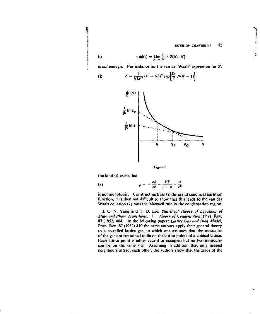
NOTES ON CHAPTER 111 75
I(i) -P•v) = Lim In Z(Nv, N)
is not enough. For instance for the van der Waals' expression for Z:
(j) Z = . (V - Nb)1 exp N(N - 1)
1# (v)
-In z
In z-
v V V2 Vo V
Figure b
the limit (i) exists, but
)b# kT a(k) p at!r. .b t,
is not monotonic. Constructing from (j) the grand canonical partitionfunction, it is then not difficult to show that this leads to the van derWaals equation (k) plus the Maxwell rule in the condensation region.
3. C. N. Yang and T. D. Lee, Statistical Theory of Equations ofState and Phase Transitions. I. Theory of Condensation; Phys. Rev.87 (1952) 404. In the following paper: Lattice Gas and Ising Model,Phys. Rev. 87 (1952) 410 the same authors apply their general theoryto a so-called lattice gas, in which one assumes that the moleculesof the gas are restrained to lie on the lattice points of a cubical lattice.Each lattice point is either vacant or occupied but no two moleculescan be on the same site. Assuming in addition that only nearestneighbours attract each other, the authors show that the zeros of the
76 REMARKS ON THE CONDENSATION PROBLEM
grand partition function all lie on a circle, and that in two dimensionscondensation occurs.
4. The first example (Eq. (20)) is due to G. W. Ford. Lee andYang (l.c. Note 3, p. 415) introduced the density distribution g(e)of the zeros on the unit circle which leads to Eq. (25) and also Eq. (28)for the b, is due to them.
CHAPTER IV
The Boltzmann Equation
I. Iutroductloa. We now will begin with the discussion of the non-equilibrium properties of gases, that is we return to the basic problemof Boltzmann: why and how is the equilibrium state reached in time.Following the historical development, I will start with the theory ofdilute gases according to the so-called kinetic method of Boltzmann,and will discuss later how this may fit into the general Boltzmann-Gibbs picture of the approach to equilibrium which was sketched inthe first chapter.
The basic equation of the kinetic method is the famous Boltzmannequation:I
(I) f= -v. -. 1+ dv I. dQ gi(g, OXf'f - ffl)
which expresses how the number of molecules
f(r, v, t) dr dv
in the element dr dv of the six dimensional phase space (p-space) of amolecule changes in time due to the streaming in is-space and due tothe collisions with other molecules. In (I) a is the acceleration dueto an outside potential U(r) and the streaming part of (I):
(2) S(f) .if - a.e I
is clearly just the local change of f per second due to the independentmotion of the molecules in IA-space. One can also say, that S(J) isthe one particle Liouville operation {H, f} with H = (p2/2m) + U(r).The last term in (I) describes the effect of the collisions; here the primeand the index I of thef's refer to the velocity variable only, so that forinstanceA =- f(r, vi, t) and the four velocity variables refer to thevelocities of the binary collision (v, v1) 4± (v', v'1); g = 1v - v1J =Iv, - v'i is the relative velocity which in a collision turns over theangle 0. To find the number per c.c. and per second of the direct
77
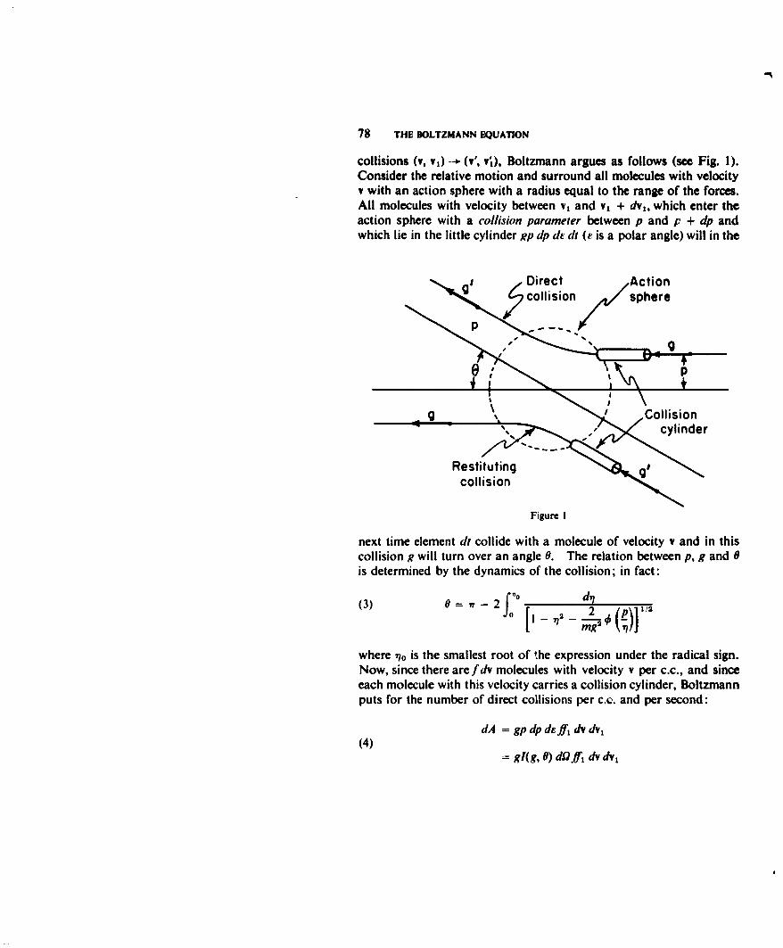
78 THE BOLTZMANN EQUATION
collisions (v, vi) - (v', vi), Boltzmann argues as follows (see Fig. I).Consider the relative motion and surround all molecules with velocityv with an action sphere with a radius equal to the range of the forces.All molecules with velocity between v1 and v, + dv1 , which enter theaction sphere with a collision parameter between p and p + dp andwhich lie in the little cylinder gp dp dE di (E is a polar angle) will in the
9._l. Direct _Action
Figure I
next time element di collide with a molecule of velocity v and in thiscollision g will turn over an angle 0. The relation between p, g and 9is determined by the dynamics of the collision; in fact:
(3) 0e= - 2f 0 1 1° :g
where 'co is the smallest root of the expression under the radical sign.Now, since there are f dv molecules with velocity v per c.c., and sinceeach molecule with this velocity carries a collision cylinder, Boltzmannputs for the number of direct collisions per c.;:. and per second:
dA = gp dp7d -ff fdv dv 1
(4)- gI(g,0 ) d2ff1-v dv2
THE APPROACH TO EQUILIBRIUM 79
where we have written:
pdpdr = I(g,9)dS?.
i(g, 0) is called the differential collision cross-section for a collisioninto the solid angle dD = sin 0 dO de. Clearly I(g, 0) through (3) isuniquely determined by the force law 0(r).
Similarly Boltzmann puts for the number of restituting collisions(v', V'*) -, (V1, v2) per c.c. and per second:
(5) dB = gl(g, 9) d.Of'fi dv' dvi.
Since the transformation from v, v, to v', v; as determined by theconservation laws of energy and momentum, is clearly a linear ortho-gonal transformation, dv dv = dv'dvi, and from (4) and (5) oneobtains therefore the collision term in the Boltzmann equation (i)since each direct collision is a loss and each restituting collision a gainin the number of molecules f dv under consideration.
Eqs. (4) and (5) express the so-called Stosszahl-Ansatz, which mayseem intuitively quite evident, but which is of course an assumptionof a non-mechanical nature. I will postpone the critical discussionof this assumption to Chapter VII. For the time being let us acceptthat the Boltzmann equation describes how the distribution functionf(r, v, t) of the molecules in 1L-space changes in time.
2. The approach to equilibrium. Since (I) is of the first order in thetime, a basic problem is the initial value problem: given the distribu-tion function f(r, v, 0) at t = 0, find the distribution at any later time.It was a great triumph for Boltzmann that he was able to show thatany initial distribution approaches in the course of time the Maxwell-Boltzmann distribution: V 2 ](6) f0 = A0 exp I-P {-' + U(r)
for sufficiently general outside potentials U(r). In here A0 and P areconstants which are determined by the given total number and totalenergy of the molecules.
Since Boltzmann's arguments are so well known, I will only sketchhis proof.
The first step is the famous H-theorem. Let
(7) H(t)= ffflogfdr dv;
80 THE BOLTZMANN EQUATION
then:"•dH f l ogfdr dv =d(H' -- +
7 jiO 8t dt ) sreaming + dt1i 'dlsions
using (I) for Of/Ot. Due to the streaming the H function does notchange. This follows from the Liouville theorem. As mentionedalready in Chapter I, §2, the integral over the whole phase space ofany function F(p) of the density of the ensemble fluid will be indepen-dent of the time. Since with independent molecules the gas is anensemble of which the density is f, one can conclude that the integralof flog f over the phase space ( = j-space) will not change with timebecause of the streaming. Due to the collisions H always decreasessince by a few simple and classical transformations one can write:2
H = !fdvfdv, f dQgf(ge)(f~fi' -ffi)In . <0
dH/dt is zero only if for all possible collisions
(8) A = f I
and this state will be reached monotonically in time. Eq. (8) deter-mines the dependence of the equilibrium distribution on the velocities.In fact the only solution of the functional equation (8) is:
(9) f Aexp{ -P!( - u))}
where A, P and the average velocity u can still be functions of r and t.From the Boltzmann equation follows that an f of the form (9) muststill fulfill the equation:
(10) If+ V .I 1= 0
and one can show that for a sufficiently general outside potentialU(r) (which include the shape of the vessel or of the wall potential),the only solution of (10) which is of the form (9) is found by puttingin (9) u = 0, P equal to a constant independent of r and t, and:
(11) A = Aoe-iv(r)
where A0 is a constant.The proof is given in Note 3. Let me only say that for special
outside potentials for instance a harmonic potential U(r) = Wr2/2, thespatial equilibrium distribution (11) will not be reached in time. Forsuch special potentials there are a host of special solutions of the
THE APPROACH TO EQUILIBRIUM 81
Boltzmann equation, in which the dependence on the velocity alwayshas the form (9) but where the A, P and u can be functions of spaceand time. Boltzmann himself gave a detailed discussion of thesesolutions (see Boltzmann, Wissenschaftliche Abhandlungen, Vol. II,p. 83). They have however only a limited interest.
Let me conclude with a number of remarks.(a) Clearly Boltzmann does not actually solve the initial value
problem stated in the beginning of this section. In fact he supposesin the first place that the initial value problem has an unique solutionand then that if at t = 0 the distribution function f goes to zero forr, v -, oo sufficiently fast for the convergence of all the requiredintegrals (especially for the total number, for the total energy and forH), then also for any later time these integrals remain convergent.From the mathematical point of view the proof of Boltzmann is there-'ore not irreproachable. For the spatially uniform case (U- 0;
f only function of v and t) and for elastic spheres (l(g, 0) = constant)Carleman has given a rigorous proof.' I will not try to indicate themethod Carleman uses, since it does not add to the physical insight.I do think though that an extension of Carleman's work especially tothe spatially non-uniform case would be quite valuable.
(b) The proof of Boltzmann does not mean, that the approach toequilibrium happens in two sharply separated successive stages: firstthe approach in velocity space to the Maxwell distribution (9) and thenthe approach in coordinate space to the "barometric" distribution (II).Both approaches are coupled to each other and the velocity distribu-tion will be strictly Maxwellian only if the complete equilibrium isreached.
(c) However it is true that the approach to equilibrium in velocityspace is quite different from the approach to equilibrium in coordinatespace. It is physically plausible and it is also suggested by Boltz-mann's proof, that the velocity distribution in any volume element ofspace will approach a local Maxwell distribution of the form (9) veryquickly and in a monotonic fashion. It will never reach it becausethe streaming and the outside forces will interfere, but it will have thistendency. On the other hand the approach to equilibrium in co-ordinate space is not monotonic in general and will require a muchlonger time. Of course this picture of the approach to the completeMaxwell-Boltzmann distribution (6) must and can be confirmed by adeeper study of the Boltzmann equation. It is the basis of a successiveapproximation method (the Chapman-Enskog development) whichwe will discuss in Chapter VI.
82 THE BOLTZMANN EQUATION
3. The Ilme'aized Doltznmnn equation. Accepting the fact that theMaxwell-Boltzmann distribution (6) will be reached in time it is clearlyof interest to investigate the case of a small disturbance of the equili-brium state. Put in (I):(12) .[ = fo[Il + h(r, v, t)]
and neglect the quadratic terms in h. One then gets the linearizedBoltzmann equation:
ag•• -. h a .h iih [ "d = - h + dr,. dgl(g, O)fo,(h' + h, - h - hi)
(13)= S(h) + C(h).
Consider first the spatial uniform case, in which there are no externalforces, so that the disturbance h depends only on v and t, and
(14) [o = n e
where the number density n and the temperature T are constants.To solve the initial value problem, it is clearly of interest to find theeigenfunctions 0, and eigenvalues A, of the collision operator C,defined by
(15) C(00) = A.01.
Some properties are quite obvious.(a) There are five zero eigenvalues corresponding to the eigen-
functions 1, v, ,2 ; this is a consequence of the five conservation laws
during a collision.(b) All other eigenvalues must be negative.PROOF.
f dvfo0 ,C(0€)
f d~and:
fdvifo•0 ,C•) = - dv f dv. f dQ gl(g, O)fofo( 1(0 + #;i - -- _,1)2
using the same transformations as used in the proof of the H-theorem.(c) Different eigenfunctions are orthogonal to each other. This
follows from:
f dvfo3•'C(/,1 ) = f dvfo0C(,).
STHE LINEARIZED BOLTZMANN EQUATION 83
(d) The operator C is an isotropic operator in velocity space and
therefore the eigenfunctions will have the form:
(16) 1,,. = R,,O,) 4,. 0)using polar coordinates in velocity space, and the eigenvalues A,, willat least be (21 + I)-fold degenerate.
Assuming that the 0, form a complete set, one can clearly solve theinitial value problem in the spatially uniform case by developingh(v, t) in the #. and one gets:
(17) h(v, t) = >_ cieAit(v)
where the c, are determined from h(v, 0). Since Ai < 0, (17) showsthat h goes to zero except for the permanent changes in density,average velocity and temperature. The quantities I /Aj clearly repre-sent a spectrum of relaxation times.
The question remains, whether such a discrete spectrum of relaxationtimes really exists. So far as I know this has not been proved ingeneral. One does knows that the collision operator C(h) is of theform:
(18) C(h) = -a(r)h + fdvlfo0K(v, vl)h(vl)
but the kernel K(v, v,) is singular, so that the usual theory is notapplicable. It is still simple to see that whatever the spectrum is, itis bounded from below, if:
fdvfa(v) = f dv f dv1 fofo, f dDgl(gO)
exists, which implies that the total cross section:
(19) Q(g) = f dQ (g,e0)
must befinite, which again follows from the physically natural assump-tion that the forces have a finite range. I believe that, in this case,the spectrum will be discrete and that the A, will approach a finitenegative limit point. But even for hard spheres (I(g, 8) = const.)this has not been proved.'
Because of these uncertainties, it is reassuring that for one specialcase the spectrum and the eigenfunctions can be determined explicitly.Since for this case we will discuss in the next chapter a special applica-tion of the linearized Boltzmann equation, I will collect here theprecise formula.
84 THE BOLTZMANN EQUATION
Going back to (13), introduce dimensionless velocity variables byputting:
S= 2Tm ) 112
and similarly for vj. Put also:
then with a = 0 (no outside fields), so that fo is still given by (14),the linearized Boltzmann equation becomes:
dh dh(20) L- + c .. = noJ(h)
with:
(21) J(h) = dc, exp(-c') dDQF(g,8)[h' + h- h - hi,V 3j\2 f fO
(22) F(g, 8) = 1/)-2 g
a is a constant of the order of the total cross section, which is intro-duced to make F(g, 9) dimensionless. I will call J(h) the dimension-less collision operator. It still has of course the same propertiesas C(h).
Now assume that F(g, 0) is a function of 0 alone. Since the relationbetween the velocities c', c€ after collision and the velocities c, clbefore collision is a linear relation, it is clear that in this case if h is apolynomial of degree n in v also J(h) will be a polynomial of degreen in v. The eigenfunctions of J will therefore be polynomia, and infact one can verify that the eigenfunctions, written again in polarcoordinates in velocity space, are:
(23) 011. = Nv.S•? 112(c2)c' Y1.(0, 40)
where the~o+ 1S 2 are the associated Laguerre polynomia (also calledSonine polynomia). Sim'(x) is defined as the coefficient of t'" in
(I - t l- -•ex I .p .I --
and their explicit expression is:
= -x (n + m)!S( ( )p!(m - p)!(n + p)!
ITHE LINEARIZED BOLTZMANN EQUATION 85
In (23) the NI, are normalization constants. The #,1,(e) form acomplete orthogonal set of eigenfunctions with weight function e-e',and the corresponding eigenvalues are:
( ,, = 21, 2f dO sin OF(O)[cos21 ! P,(cos.)(24) f c 2 2
+ sin2'IPg(sif I - -8, 8,
Eqs. (23) and (24) were found first by C. S. Wang Chang and then alsoindependently by L. Waldmann.' Note that the five zero eigenvaluesare Aoo, A•o and Ajo corresponding to the eigenfunctions I, c and(3/2 - c2). One further sees from (24) that the A,, converge for larger and I to:
(25) - 2,r fo dO sin OF(O)
which we can assume to be equal to - I by the proper choice of a.I will call this special case of the linearized Boltzmann equation the
quasi-Maxwell model. It is not a realistic model, in the sense thatthere is no intermolecular potential for which F(g, 0) depends only on0 and for which the integral (25) converges. When the force is equalto Kr- (Maxwell model),
gl(g, 9) = W FM()
but for small 0, F,,(O) - 0'2 so that (25) diverges, correspondingto the fact that Or) has an infinite range. I However, it seems to methat the quasi-Maxwell model must be quite similar to the actual caseof forces with finite range, and will give therefore at least a qualitativeinsight.
Finally let me point out, that in (19) the order of magnitude of theeigenvalues of the collision operator noJ(h) is clearly no, whichcorresponds to the order of magnitude no(kTIm)" 12 for the eigenvaluesA, of C(h). Thus (A,) - ' is of the order of the time between collisionswhich confirms the view that the Maxwell distribution will be reachedafter a few collisions, that is in a time of the order of the time betweencollisions.
NOTES ON CHAPTER IV
I. For the complete discussion Boltzmann's book Vorlesungen uiberGastheorie (Ambrosius Barth, Leipzig, 1912) is still indispensable.See esp. Vol. 1, Part II, and Vol. 2, Part Vii.
2. One has:
(7t = f d f dvi f d.gI(g, 0) Inf.(f'f1 ' - ifs)
= f dv fd, f digl(g, O)Inf,(f'f; -iff),
by interchanging v and vi. Therefore, adding the two expressions anddividing by two:
= I f dv f dv fdQ gl(g ff' - ff,)lIn (ff")
= 'f dv f dv, f dQ gl(g, O(ff. - f'fl') In (f fr),
by interchanging the velocities before and after collision and usingagain dv dv, = dv dv. Adding the two expressions and dividing bytwo leads to the form given in the text.
3. Write Eq. (9) in the form:
InJ= -hr 2 + kyv + n
so that h = #m/2, k = nif•u and n = In A - Pmu'/2. Substituting in(10) and requiring that (10) must be fulfilled identically in v leads tothe equations:
(a) 0, =0,
(b) Lk-+ kj - 2 M 8 = 0,
4~k i~n(c) '-! + - - hai = 0,
{d) can(d) T+ k+aa = 0.
86
INOTES ON CHAPTER IV 87
From (a) and (b) one concludes that h can only be a function of thetime and that
dh(e) k = ko(t) + [120) x r] + h r.
At this stage one can say therefore that the average motion of the gascan only be a possibly time dependent combination of a translation,rotation and a radial expansion or contraction. Since ma---grad U(r), it follows from (c) that:
()k grad n + U •
Therefore the curl of 1k/0t must be zero, which implies that 12 mustbe a constant and then it follows from (e) and (f) that:
2idko Ild2hn h +ýU = no(t) -do- r - f-h r2.
m d - 2dt2
Substituting this expression for n in the last equation, (d), which hasto be fulfilled, leads to:(g) k.grad U + h no -d2ko-- I dr3h 2 .
m mdt' dt dt2 2 dt3
Now suppose that from an arbitrary origin the outside potential U(r)can be developed in a power series:
(h) U = A.x + A• Axx + X AayxaxOxY
where the A's are known constants. Higher order terms will beneglected since it will turn out that with arbitrary A's the form (h) hasalready sufficient generality. Introducing (h) in (g), it is clear thatonly the left hand side will contain terms of the third degree in the x,.Equating the coefficients of these terms to zero gives ten homogeneouslinear equations in the four unknowns dh/dt and 2l. Thus one findsthat in general h must be constant and $2 = 0. From the terms ofthe second degree in the x,, one then can conclude that llso ko = 0,so that k is zero all together. From (d) follows, that then n must beindependent of the time, and from (c) one concludes that n + 2hU/m =
no which is equivalent to Eq. (II) in the text.
4. T. Carleman, Probikmes Mathematiques dans ia Thiorie Cindtiquedes Gaz (Publications Scientifiques de l'lnstitut Mittag-Leffler, Vol. 2,Uppsala, 1957). The generalization of the proof for other force lawswith a finite range is straightforward.
88 THE BOLTZMANN EQUATION
5. This was first shown by D. Enskog, Kinetische Theorie derVorgange in Massig Verdfinnten Gasen, Dissertation, Uppsala, 1917,p. 140. For a more transparent proof see L. Waldmann, Handbuchder Physik 12, p. 366.
6. There is also the following troublesome question. Should oneimpose the condition that the integral:
(i) f dVfo
exists in order to select the eigenvalues and eigenfunctions of the linearcollision operator C(o)? On the one hand this is necessary if onewants to apply the usual Hilbert space theory. But on the other handthe integral (i) has no physical meaning in contrast to the case ofthe quantum mechanical operators. This difficulty was noticed byN. G. van Kampen (Physica 21 (1955) 949; see especially the remarkson p. 957). L. Waldmann (Handbuch der Physik 12, p. 365 and p. 367)has tried to connect the square integrability condition with the require-ment that the entropy should always exist. However his argument isnot convincing.
7. C. S. Wang Chang and G. E. Uhlenbeck: On the Propagation ofSound in Monatomic Gases. Report of the Engineering ResearchInstitute, University of Michigan, 1952. L. Waldmann, Handbuch derPhysik 12, §38.
8. Explicitly one finds (see Maxwell, Collected Papers, Vol. 11, p. 42):
I (cos 20)1'2F.(O) = � sin 0 sin 20 {cos2 4K(sin 0) - cos 24)E(sin 0)}
where 4) is related to 0 by:
2 = (cos 20)1' 2K(sin 4).
K(x) and E(x) are the complete elliptic integrals of the first andsecond kind respectively. FM(O) is a monotonic decreasing functionof 0; for small 0:
F 3•(O ) 113')2 (Si 35 )(6 0 1 + 27 ...
while for 0 = 7r:
FM(-) - 4K2(1/4) 0.0727...4 (w4
CHAPTER V
The Propagation of Sound
I. Introduction. As an application of the linearized Boltznannequation let me consider the propagation of sound in a gas. Clearly,if the gas is in equilibrium and if the intensity of the sound is not toohigh, then the sound waves will be a small disturbance from equili-brium and should therefore be described by the linearized Boltzmannequation.
First let me tell you some of the experimental facts.. The firstquestion is how fast sound propagates, and the answer seems withoutmystery and is known to every physics student. He knows that thevelocity Vo depends on the adiabatic compressibility of the gas andthat one gets:
(I) = (-, L112 = (5k k)'12
for a mono-atomic gas, to which I will always restrict myself. How-ever, if one does not look upon the gas as a macroscopic material withsome compressibility, but as a collection of almost independentmolecules, then it seems to me that the sound propagation becomesmore mysterious. How is it possible to impose on the random motionof the molecules the ordered motion, or in present day terminologythe collective mode of motion, which a sound wave represents? Thatone runs into rather deep questions becomes apparent, when onewants to find the frequency dependence of V, the dispersion of sound,and the accompanying absorption of sound. Since the days ofKirchhoff one knows that for increasing frequency, V becomes larger,and absorption sets in. The latter can still be partially understoodfrom the macroscopic point of view. At high frequency the tempera-ture and velocity gradients between compression and rarefactionbecome so steep that although the time between them gets shorter, theheat conduction and the viscosity of the gas begin to have effect andcause absorption. Kirchhoff found for the absorption coefficient inamplitude:
89
90 THE PROPAGATION OF SOUND
(2) ct (2 0+ m)
where to = angular frequency, p the density, IA the viscosity coefficientand K the heat conduction coefficient of the gas. Note that sinceK - (k/re)J,, u - pAlc> with A the mean free path, ýc> some averagethermal velocity (hence , c> - Vo), (2) shows that a0 - A/A2 if A isthe wave length of the sound. Experimentally (2) has been wellverified, whcn the frequency w is not too high.
What happens if the frequency gets higher and higher? The mostextensive experiments have been done by M. Greenspan for heliumgas.' His method was the usual one, although many precautions andrefinements were necessary of course. A piezoelectrically drivenquartz plate A produced the sound waves and the density fluctuationswere picked up at an identical receiver quartz plate B producingvoltage fluctuations which then could be amplified. The difference inphase of the fluctuations between A and B determines the phasevelocity and the ratio of the amplitudes gives the absorption coefficient.The distance L between the plates was always much larger than themean free path A. The results seem to indicate that the velocity Vand the absorption coefficient a increase monotonically with frequency.The highest value of A/A which could be realized was of order oneand the velocity V had then increased to about 3 V0, while the absorp-tion coefficient had become of order I/A, so that the absorption wastremendous.
What happens for ,-r. ? Some people have speculated that Vand a might become infinite, since practically infinite velocities occuraccording to the Maxwell distribution. Others have thought that Vmight become constant again while the a goes through a maximum,similar to the observed behaviour in poly-atomic gases. But there isno real reason for either belief.
2. The Wasg-Chang method. Returning now to the theory, to findthe dispersion law of the sound waves it seems natural to seek a solu-tion of the linearized Boltzmann equation (see Chapter IV, §3):
i•h i'h-- + c.-- = 11,J(h),
(3)J(h) = :- 2 f dc, e-1f d F(g, 0)[h' + h' - h - hi]
which has the form of a plane wave, say in the :-direction. Puttherefore:(4) h = exp[i(kz - wor)]ho(c)
THE WANG-CHANG METHOD 91
where o0 = w(m/2kT)1 12 and k = 2w/A is the wavenumber (not to beconfused with the Boltzmann constant k which occurs always in thecombination kT). Now develop ho(c) in the eigenfunctions of J(h):
ho(c) = al a,(c).
One clearly gets an infinite set of linear equations
(5) ik > Mi• a. - iwoal = noA•la
with:
(6) Mi. = f dc c..,•,ec
The equations (5) will have a non-trivial solution only if the infinitedeterminant of the coefficients vanishes. This condition:
(7) iikMj,,, - (iUo + nAi)81m11 = 0
gives a relation between wo and k and hence expresses the dispersionlaw of the gas. However. the discussion is hard. All that we couldthink of was to break off the determinant successively. It is simpleto see that taking only the first three rows and columns, correspondingto the three zero eigenvalues (for which the eigenfunctions are !,c. and c2 - 3/2, so that the corresponding elements of M1,, are simpleto evaluate), leads to the cubic equation:
W(W 0 ~k ) = 0
with the three roots ,o0 = 0, too ± k(5/6)1 2 The last two rootsclearly represent "propagating" modes going to the right and leftwith the velocity:
_ = O (2kT)12 = (5 kT)l2
so that we have derived Eq. (I). By taking more rows and columnsone gets higher order algebraic equations in a, 0 , and by then followingthe propagating modes (that is the roots which for k --) 0, become± k(5/6) 2 ) one can see what happens for larger k or smaller wave-lengths. This is straightforward for the quasi-Maxwell model, and
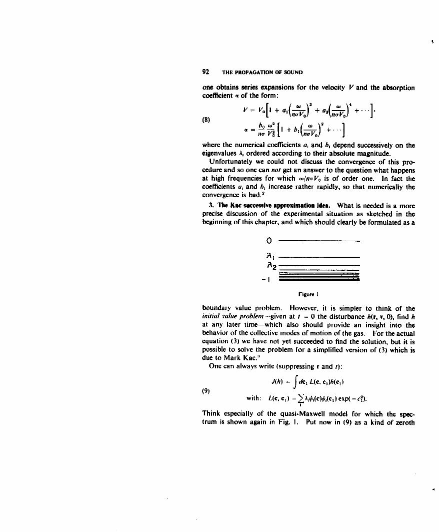
92 THE PROPAGATION OF SOUND
one obtains series expansions for the velocity V and the absorptioncoefficient a of the form:
()V v0 I + a,( r) 2 + a2( '" )4(8) oVnoO
a - I b[ +b
where the numerical coefficients a, and bi depend successively on theeigenvalues A, ordered according to their absolute magnitude.
Unfortunately we could not discuss the convergence of this pro-cedure and so one can not get an answer to the question what happensat high frequencies for which v/nVo, is of order one. In fact thecoefficients a, and b, increase rather rapidly, so that numerically theconvergence is bad.2
3. The Kac successive approximation idea. What is needed is a moreprecise discussion of the experimental situation as sketched in thebeginning of this chapter, and which should clearly be formulated as a
0
A2
- I
Figure I
boundary value problem. However, it is simpler to think of theinitial value problem-given at t = 0 the disturbance h(r, v, 0), find hat any later time-which also should provide an insight into thebehavior of the collective modes of motion of the gas. For the actualequation (3) we have not yet succeeded to find the solution, but it ispossible to solve the problem for a simplified version of (3) which isdue to Mark Kac.3
One can always write (suppressing r and t):
J(h) = fdc, L(c, ci)h(c,)(9)
with: L(c, cl) = ý•A•,(c)0,(c 1 ) exp(-c2).
Think especially of the quasi-Maxwell model for which the spec-trum is shown again in Fig. I. Put now in (9) as a kind of zeroth
THE KAC SUCCESSIVE APPROXIMATION IDEA 93
approximation all At = -1, except the 5 zero eigenvalues. In firstapproximation one would then keep the first negative eigenvalue A, andcollapse all others in - I, and so on. At every stage one can solve theinitial value problem and one can also discuss in detail all the normalmodes, because the linearized Boltzmann equation now becomes anintegral equation with a degenerate kernel. In fact using the com-pleteness relation of the 0,, one gets in zeroth approximation from (3)and (9):
(10) + nh +c.
= 13 fi I + 2c]c + 2(c2 - 2
and this should also be the zeroth approximation for any molecularmodel for which the range of the forces is finite.
To simplify the algebra as much as possible I will discuss instead of(10), the equation:
(11) - + Yh + c~x = Y dc, exp(-c2/2X)( + ccl)h(cl)e'x (2w)' f~
which is a kind of one-dimensional version of (10). It is related to aone-dimensional Boltzmann-like equation, which was also proposedby M. Kac and it can be obtained by a mutilation of the linearizedform of this equation." The mathematics of (10) and (I1) are quitesimilar and also the results are similar, but everything is much simplerfor (II).
Since in (II) the coefficients are independent of x, one can alwaysmake a Fourier transformation in x. Put:
hk(c, 1.) = e" e|"ih(x, C, 7);
then 01I) becomes:12) L + (Y + ikc)hk = 2 dc, exp( - c2/2)(I + cc,)hk(cl, ).
To solve the initial value problem one can use two methods:(I) the Laplace transform method in r, which brings in immediatelythe initial value of h,, or (2) the method of normal modes, in which theinitial distribution must be developed (provided the normal modesform a complete set) and from which the further temporal develop-ment then follows immediately.
94 THE PROPAGATION OF SOUND
Of course, if you do it right the two methods will always give thesame answer. I will give some details of both methods, mainlybecause for the quite analogous problem of plasma oscillations therehas been some confusion in the literature which only recently has beencompletely dispelled by K. M. Case (Ann. Phys. 7 (1959) 349). Beforeembarking on this, note that from (II) still follows by multiplyingwith e- 2/2 and integrating over c:
(13) Lp + 0
with
p(x, 7) = de e- 2 12h(x, c, 7),
(14)
OX(x, 7) = J e dce-c"2 ch(x, C, 7)
or after a Fourier transformation in x in obvious notation:
(!5) t____) + ik~k&7) = 0.
Eq. (13) is a kind of continuity equation or macroscopic equation forthis model.
4. The Laplace transform method. Put now:
h,,(c) = D dr e- "'hk(c, 7);
then one gets from (12):
(16) (p + y + ikc)hk.P = hk(c, 0) + 12 (pt, + c~kP).
But from (15) follows:
Okkv = ;k [Pk(O) - Pkl
Put this in (16), then:
hkP hk(c, 0) ,Pk(O) + + YPkp I - cp/ikp + y + ikc +ik(2n)"p + y + ikc (27) 112 p + y + ikc
THE LAPLACE TRANSFORM METHOD 95
Multiply with exp(- c2/2) and integrate over c. One then gets a trapfor pk, and one finds:
Mh(c, 0) + (2 Pk(O)(18) PkPGpk)f, dc ik(2ir)11 e- 2 /2
G(p, k), p + + ikc
with:I• - cp/ik 212,
G(p, k) = I Y /2 dc e-c(21")l'= f. p +' y +kce
This put in (17) determines hk, completely in terms of the initial datahk(v, 0) and pk(O). In fact once p(x, -) is known by inversion of (18),it is quite easy to invert (16) and one finds:
h(x, c, 7) = e "-h(x - cv, r, 0) + (2 / dr' e- '"(19) 2lI
x [p(x - ,-', 7 - r') + c4(x - ,-,',r -v ')].
This shows that the influence of the initial distribution damps outin time and that for large 7 the distribution function h(x, c, v) dependsonly on the "macroscopic" quantities p and 0.
5. The normal mode method. This method is perhaps more physical,and anyway it is more familiar. Go back to (12) and seek solutions ofthe form:
hk(c, 'r) = hok(c) e-
The function hk((c) is the eigenfunction or normal mode correspondingto the eigenfrequency w. One gets from (12):
(20) (-iw + ), + ikc)h,,k = (2 )(Pk + C0.0
and from (15):
(21) Wpk = kO.A
Because the equation (20) is homogeneous in hk, one can alwaysnormalize ho, so that:
(22) poik = f 7M dc e -hM(c) I
and then from (20) and (21) one gets:
(23) (- + y + ikc)h,,k •( ! + ) ( 0c
% THE PROPAGATION OF SOUND
Now one has to watch out! From (23) one can only conclude:
(24) hk(C)+iY+ ( 12 1 +wclkk ) (2,r)'1 ikc - io + y
where A is arbitrary. To find the spectrum of eigenfrequencies w,one has to distinguish two cases:
(a) e = (w + iy)/k is real. Then from the normalization condition(22) one gets:
I =f 2+ dc I + 'c/k e-C2 /I A-Cas +ik(2,')1'I c - e
where the principal value of the integral is meant. This determines Aand hence for fixed real k, there is a continuum of complex eigen-frequencies all with imaginary part equal to -iy. For these modesone can not speak of a dispersion law since there is no relation between
and k.(b) e is not real. Then since c is real, one can omit in (24) the
&-function. From the normalization condition one then finds:
(25) 1= 2"f: dc I + `C/ke-C2 Y2 .ik(2,0)',f c-
The right-hand side is an analytic function of w (always for fixed real k)everywhere, except on the line where the imaginary part of W is -iy.Hence (25) can only be fulfilled for a discrete set of values of wa (whichmay of course be the null set) for each value of k. For these discretemodes there is therefore a dispersion law, and they are the collectivemodes among which there must be the sound propagation.
The connection between the two methods is clear. The modes arethe poles in the p-plane in the expression (18) for the Fourier-Laplacetransform of the density p. Especially Eq. (25) is just the equationQ(--iw, k) = 0. I will therefore not further elaborate on the deriva-tion of the solution of the initial value problem by means of thenormal modes.
Because in this simple case the Eq. (25) for the discrete modes isquite explicit and simple, it is possible to find the discrete modes andto follow them as functions of k. Put:
:=wf/k, x = y/k, C = : + ix,
F(C) = /2 dc e - c2 12
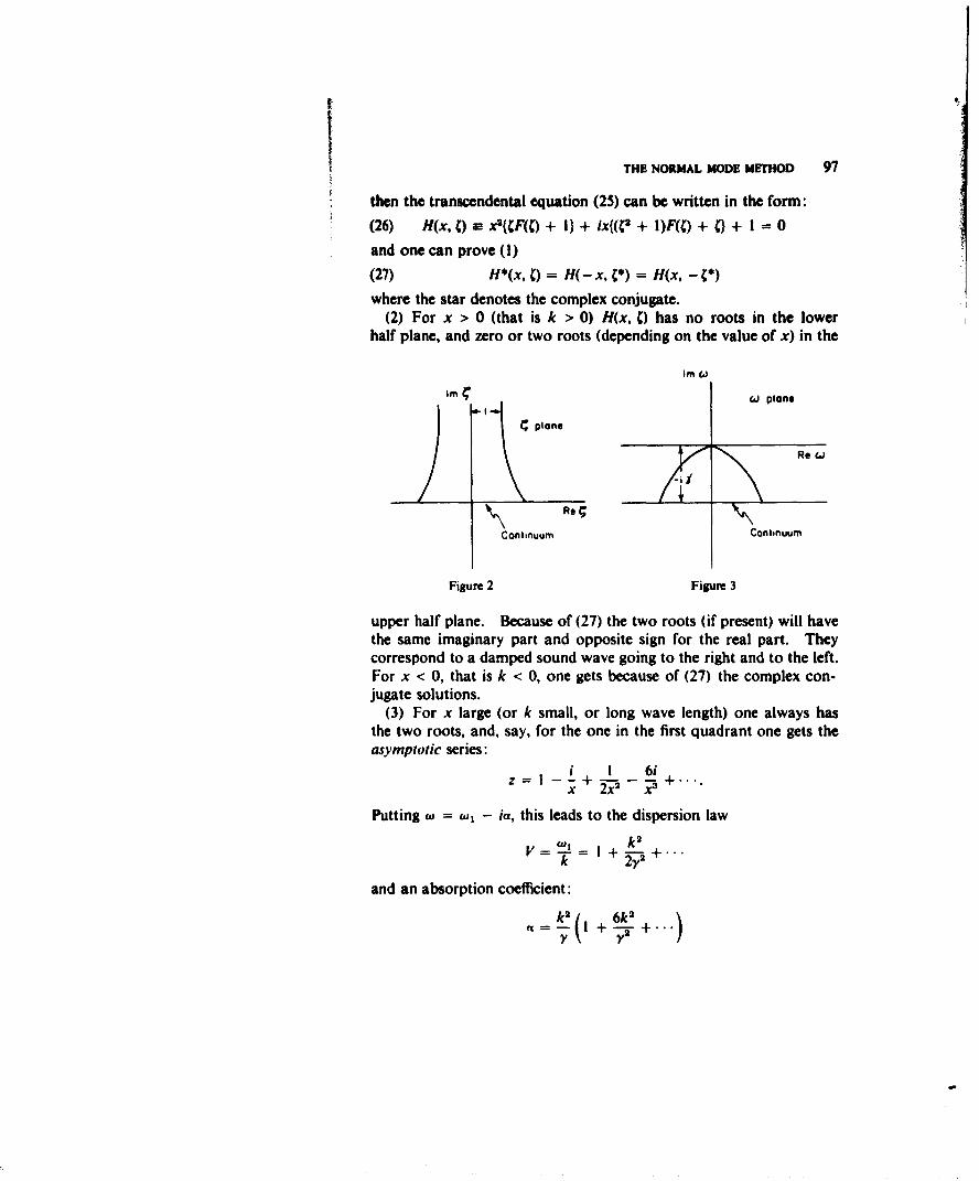
THE NORMAL MODE METHOD 97
then the transcendental equation (25) can be written in the form:
(26) H(x, C) - x2{(F(C) + 1) + ix{(( 2 + I)F(C) + C) + 1 = 0
and one can prove (I)
(27) H*(x, ) = H(- x, C*) = H(x, - 4*)where the star denotes the complex conjugate.
(2) For x > 0 (that is k > 0) H(x, C) has no roots in the lowerhalf plane, and zero or two roots (depending on the value of x) in the
Im .)
Im C. plane
Spiano j~jj( Re
\ Re 1;Continuum Continuum
Figure 2 Figure 3
upper half plane. Because of (27) the two roots (if present) will havethe same imaginary part and opposite sign for the real part. Theycorrespond to a damped sound wave going to the right and to the left.For x < 0, that is k < 0, one gets because of (27) the complex con-jugate solutions.
(3) For x large (or k small, or long wave length) one always hasthe two roots, and, say, for the one in the first quadrant one gets theasymptotic series:
i + I 6i- 2X2 ? •
Putting w = ,- ia, this leads to the dispersion law
V wI k2
and an absorption coefficient:
k ( +6k2+)V V
98 THE PROPAGATION OF SOUND
which are similar to the series expansions (8) and which are in factidentical with what one would obtain by applying the Wang-Changmethod to Eq. (II).
(4) For decreasing x (or decreasing wave length) V and a increasemonotonically till x = xcrit = 0.724. .. For x < Xcrit there are nomore discrete modes. The paths of the two roots are shown in Fig. 2in the C-plane and in Fig. 3 in the w-plane. The velocity increasesabout 10% and the damping increases until it has become as large asfor the continuum modes. A similar discussion can be carried outfor the more realistic three-dimensional equation (10). The normalmode spectrum consists of a continuum for which the imaginary partof w,, is equal to -no, and three discrete modes if x = na/k is suffi-ciently large. For x - ' , these modes correspond to z = wo, k = 0,± (5/6)Y 2, which are the same as found by the zero approximation ofthe Wang-Chang determinant (7). For smaller x or shorter wavelength one obtains series expansions like (8) for the propagatingmode but now one can prove that these series are asymptotic. Thethird mode, that is the one for which z becomes zero for x -* oo,always is purely imaginary and is not a propagating mode. It canperhaps be called a diffusion mode. There is again a critical value ofx for which the damping of the propagating modes has become n,so that they then merge with the continuum. The paths of the discretezero's seem more complex and need further investigation. It maybe that V as function of k will go through a maximum before thecritical value of k is reached.
From the physical point of view, it seems to me that the qualitativefeatures of the results, namely: the existence of the continuum (or ofsingle particle modes), sound as one of the discrete modes, the existenceof a critical frequency for the sound modes are probably general andare physically reasonable consequences of the existence of a totalcross-section; that is, of a lower bound of the spectrum of relaxationtimes. I am very hopeful that it will lead to a real explanation ofwhat sound is at very high frequencies and will help to explain theGreenspan experiments and perhaps will suggest other experiments.

NoT•s ON CHAPTER V
1. M. Greenspan, J. Acoust. Soc. Am. 22 (1950) 568. In theactual experiments the frequency of the sound was kept fixed and themean free path A was varied by changing the pressure of the Heliumgas. Since the relevant parameter is A/A this is equivalent to changingthe frequency while keeping the pressure of the gas constant. Therestriction to mono-atomic gases should be emphasized. For poly-atomic gases there is an additional cause for the dispersion andabsorption of sound, which is due to the lag in the transfer of thetranslational energy into internal energy, and which usually completelymasks the dispersion of sound with which we are concerned here.
2. For the detailed discussion we refer to the report cited in Note 7,Chapter IV. The calculations were done for the real Maxwell model.Since in this case there is no total cross-section o, another form forthe dimensionless parameter of order A/A in the development is needed.We chose sW/p V2o, where IA is again the viscosity coefficient. Theresults were:
I- 215 ~j 41.15.10i (Itv )4 }
2.99 1"" )2 + 56.7 ("w)}"
iw2 {7 51 5 5 (•j +"'}
-Pw I.2-• 11.9( j_)2 +..
which shows how fast the coefficients increase.
3. None of this work has as yet been published. A joint publica-tion is in preparation.
4. The one-dimensional Boltzmann-like equation proposed byM. Kac (Proceedings of the Third Berkeley Symposium on Mathe-matics, Statistics and Probability, Vol. 3, pp. 171-193) has the form:iof 3ff _ f r
-L + v ±f v dvi dO F(O){f(x, v', t)f(x, r', t)(a) a - f(x, r, t)f(x, v1, t)}
99
100 THE PROPAGATION OF SOUND
where v' = vcos9 + vsin0, v, = -vsin9 + vicos, and whereF(M) = F(-9) is a dimensionless "collision" probability. Just asthe real Boltzmann equation it leads to an equilibrium distribution:
fo = A e--v2
and by linearizing, putting f = fo(I + h(x, v, t)), one obtains:
+ h vhS+ c = vAJ(h),
(b)J(h) = dc, exp( - c0/2) f dO F(O)(h' + hi - h - h1)
with c = v(29)112 and i- = t(20)112. It is easy to show that the eigen-functions of the dimensionless linear operator J(h) are the Hermitepolynomials H.(c) (also sometimes written He.(c), since the weightfunction is exp( - c2/2)) and that the corresponding eigenvalues are:
(c) A. = (21r), 2 f" dO F(0){(cos 8)1 + (-, )n(sin 0) - I - 8.0
In terms af the eigenfunctions one can write J(h) in the form:
(d) JMh) f dc, L(c, cl)h(cl)
with:
L(c, cl) = X H2(c)H.(,) exp(-c•/2)
which is similar to Eq. (9) of the text.The mutilation of the linearized equation starts from the form
(d) of J(h). Putting A0 = A, = 0 and all other eigenvalues equal to-y/MA leads to Eq. (II) of the text. It should be pointed out that this
mutilation is not analogous to what was done in the three-dimensionalcase, because from (c) follows that AO = A2 = 0, while all othereigenvalues are negative and converging to:
-(2n) 1 /2f dO F(8).
In the Kac successive approximation method applied to (d) one would
NOTES ON CHAPTER V 101
put therefore in zeroth approximation Ao = A2 - 0 and all othereigenvalues equal to -y/vA. This leads to the equation:
Sh ,~h = ' I'-+ yh + col' ( = 1 - dc, exp-c•/2)
x{+ ( -I)(_ l)}h(ci).X f I+ (C2 _I)C2-
However it can be shown that this equation does not lead to collectivemodes which are similar to sound.
CHAPTER V!
The Chapman-Enskog Development
I. Introduction. We now return to the general non-linear Boltzmannequation:
+/ V.f +a.• d, .I d. gl(g, 0)[ f 71' -. ff,]I(I) - +. f f
discussed in Chapter IV, and we will consider the general problem ofhow the usual macroscopic description of the gas in terms of thehydrodynamical equations is contained in the Boltzmann equation (I).This problem has a long history and both Maxwell and Boltzmannhave given it a great deal of attention. The first completely satis-factory solution was given in the dissertation of Enskog in 1917, whichwas inspired by Hilbert, and independently by Chapman, who usedanother method which goes back to Maxwell but which led to thesame conclusions.' I will only try to sketch this theory, and I wantto emphasize the mathematical features, which I think are quitecurious and fundamental. From the physical point of view, thistheory constitutes one of the t'ew successful descriptions of a class ofnon-equilibrium phenomena in terms of the intermolecular forces.
2. The general conservation laws. The first step is to derive from(I) the so-called transport equation for a quantity 4,(v) which a mole-cule can carry "on its back". Defining:
(2) t)"f =~- n(r f)= =-Jv•fdvf n
where n(r, ) is the number density, one gets from (I) by multiplyingwith 0 and integrating:
+ (n ) - na TO(3) x
S f A dvfdv i f diQgl(g, OX + 0, - 0'- 0)[f:f' - ff]
102
I
THE GENERAL CONSERVATION LAWS 103
where in the collision term the same transformations, used in the proofof Boltzmann's H-theorem (see Chapter IV, Note 2) are used again.Take now for 0(y) successively the five quantities I, v, v2 which areconserved in a collision. For these the right-hand side of (3) vanishesand after a few simple transformations one can write the resultingfive equations in the form:
(a) at+ j(.u 8 ) = 0,
Du, 1 uu, , pa -P:.
(4) (b) p D - L, + U. ý-'• pa, -
(c) -D t -) + iq.=
where we have used the index notation with the usual summationconvention, and where:
p(r, t) = mn = the mass density;
u,(r, 1) = fj = the average velocity;
U, = I-I = the thermal velocity;
Q(r, t) = p = the thermal energy density;
P,,(r. 0) = pUtUj = the pressure tensor (obviously
symmetric);
qfI, 0 pU2- = the heat current density;
D,, = I ,L-. + LU, = the rate of strain tensor.
The equations (4) express the conservation laws of mass, momentumand energy.2 They are a rigorous consequence of the Boltzmannequation, but of course they are still an empty frame, since we do notknow how to express the P, and the q, in terms of the average flowvelocity, the density and the temperature. Or, in other words, onestill has to derive the Newton and Fourier phenomenological laws forthe friction and the heat conduction.
3. Tim Cbapman-Emskog developmemt. To do this one has somehowto solve the initial value problem for the Boltzmann equation, since tofind the average values P,, and q, one must know the distribution
104 TIlE CHAPMAN-ENSKOO DEVELOPMENT
functionf Now we discussed already in Chapter IV that the approachto equilibrium proceeds so to say in two stages. Because of thecollisions any initial distribution will reach very quickly (in a time ofthe order of the mean free time to AI/(kTIm) 112) a local Maxwelldistribution:
(5) f(o) = m 3 -2 M -U)
where the macroscopic variables n, u and T are still functions of rand t. In the second stage the slow relaxation of the macroscopicvariables to their equilibrium values takes place, and it is this stagewhich we want to follow in more detail. Now the argument goes asfollows:
I. First note that if one uses (5) to calculate Pil and qj one gets:3
q, 0 , Q = p,
(6) P =p8,, with p= nkT
so that (4) becomes:
(a) + div(Pu) = 0,
Do(7) (b) p 5t = p - grad p,
(c) D (pT-312) = 0
which are the ideal, or Euler hydrodynamical equations with adiabatictemperature changes and with an equation of state which is still theideal gas law.
2. Of course the two stages of the relaxation to equilibrium are notsharply separated, so that one must not expect that after a time oforder to the distribution function is precisely of the form (5). Insteadit seems more reasonable to put in Eq. (I):
(8) f = fP° [V + 00r, r, t))
and to keep in the collision term only terms linear in 0. Finally,since it is the streaming term in (I) acting on n, u and T which causesthe deviation 0 from the local Maxwell distribution (5), it is sufficientto put only f(°) in these streaming terms. Thus one is led to:
(9) + I'-, + a,
THE CHAPMAN-ENSKOG DEVELOPMENT 105
where:
() = fA,,io) fdD g(g,e)[0' + #; - 0 - 0,1
is the same linearized collision operator introduced in Chapter IV.Note however the different way in which one now has linearized theBoltzmann equation. The resulting equation (9) is an inhomogeneouslinear integral equation, in contrast to the homogeneous equationdiscussed in the previous chapter.
3. One now runs into the following trouble. The homogeneousequation C(#) = 0 has the five solutions I, v, and v1 (which I willcall #,), and therefore (9) has in general no solution. The solubilityconditions are that the left-hand side of (9) must be orthogonal to the0, and these five conditions turn out to be the Euler equations (7) forn, u and T with p = nkT.3 These equations allow us to express thetime derivatives of the macroscopic variables in terms of their spatialderivatives and doing this one then finds: 4
+ _l• , + a. , P)[1' T U.(M V2;
(10) + ( -U 2
I •Dn U.U# - 1 ,S.'U2
where U, = v, - u, is again the thermal velocity. With (10) for theleft-hand side of (9), this equation has a solution of course, which isalso unique if we require that:
(II) fdv ,f0,+)O =0
which means physically that the macroscopic variables must always bedetermined from -O) alone.
4. With the solution for q, one then can calculate the pressuretensor P1, and the heat flux q, for which one finds the well-knownNewton and Fourier laws:
P., = pS, - 2.(D,, - D.S,,(12) bT
q, = K FX,
but with known values for the viscosity and heat conduction coefficientsft and K. Putting (12) into the general conservation laws (4) thenleads to the Navier-Stokes equations of hydrodynamics.
106 THE CHAPMAN-ENSKOG DEVELOPMENT
4. Solutoim of the Integral equatio (9). To find the solution for 0 isthe hardest part of the theory. To give you some idea how it goeslet me consider again the quasi-Maxwell model. Since the right-handside of (10) and also fb°) depend only on the thermal velocity U,, 0will also depend only on U,. Using dimensionless velocity variables:
C= m ,) 2 U.
Eq. (9) becomes:
(13) 1. C(2 + 2D.,( m--) (C.C- 8,,C2 n )
with: I f , ,-fýJ(W) = ; 3 , 2 fdce f dQF(O)[0' + Ol-1'-#1.
The conditions (II) are equivalent to:
(14) fdc{ e- C2(c) = 0.
Eq. (13) is especially simple for the Maxwell model, since the functionsc,(5/2 - c2) and cc, - (1/3) 8 ,,c2 which occur on the left-hand side of(13) are eigenfunctions of the operator J(O~). In the notation ofChapter IV they are 011m (with m = 0, ± I) and #02. (with m = 0,± I, ± 2). Since furthermore I, c, c2 - 3/2 are the eigenfunctions
Oooo, #o0. and Ooo a linear combination of the functions 0,,. ando02, will also fulfill the condition (14). Hence one easily sees that an
exact solution of ( 13) is:
(15)0(c) = I I iT(x, c 2 -) + 2 1 12
. Da.N(C.C - .8.OC2)
where the eigenvalues A,, and A0 2 can be found from the generalformula (24) of Chapter IV. This formula gives:
(16 o2 = - •fdt2sin3 OF(O).
!SOLUTION OF THE INTEGRAL E.QUATION (9) 107
One then finds:
qi= U pU 2 = v (2 k dc e-c1 4(C)cjc
+2nkTPil =PUNY = p811 + W 31 fde e-•ccc
-=pst + ý (D., - D .. 8,)•expresons ofthe 4 A02 (9(0
One gets therefore the Fourier and Newton laws (12), and one obtainsfor the heat conductivity and the viscosity coefficients the explicitexpressions:
5 ink /2k T 112 m (2.k _1,2'(17) ; A, - '- J )A• 2 " 0o2
which are both positive since All and A.2 are negative. Both areindependent of the density and, therefore, functions of the temperaturealone. The independence of density is one of the classical results ofthe kinetic theory of gases and is in accord with experiment. Thetemperature dependence is different for different molecular models.The dependence - V ;2 which holds according to (17) for the quasi-Maxwell model (if (Y is taken independent of T), is also valid for theelastic sphere model.' It only agrees qualitatively with experiment.
From (17) one still finds:
15 5(18) K = 1- k C, = C,
which is confirmed very well for mono-atomic gases; 5/2 is the so-called Eucken constant.
Also for other molecular models, in fact for an)' differential cross-section I(g, 0) it is possible to find the solution of the integral equation(9). The best method (first suggested by Burnett) is to develop 0always in the eigenfunctions 0,,. of the Maxwell model. For thecoefficients one then gets an infinite set of linear equations, which canbe solved successively and at least for repulsive forces inverselyproportional to some power of r, the convergence of this procedurehas been established.'
It should be emphasized that one thus obtains ,K and ut expressedexplicitly in terms of I(Ag, 0) and hence in terms of the force law. One
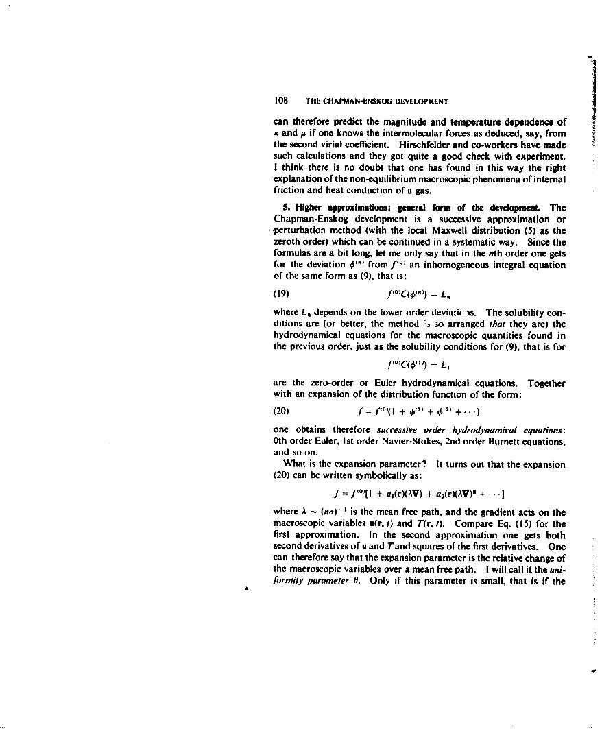
108 THE CHAPMAN-ENSKOG DEVELOPMENT
can therefore predict the magnitude and temperature dependence of,c and is if one knows the intermolecular forces as deduced, say, fromthe second virial coefficient. Hirschfelder and co-workers have madesuch calculations and they got quite a good check with experiment.I think there is no doubt that one has found in this way the rightexplanation of the non-equilibrium macroscopic phenomena of internalfriction and heat conduction of a gas.
5. Higher approximations; general form of the development. TheChapman-Enskog development is a successive approximation or-perturbation method (with the local Maxwell distribution (5) as thezeroth order) which can be continued in a systematic way. Since theformulas are a bit long, let me only say that in the nth order one getsfor the deviation 0'"' from f,0) an inhomogeneous integral equationof the same form as (9), that is:
(19) f'0 )C(W) = L.
where L. depends on the lower order deviatic as. The solubility con-ditions are (or better, the method :s ;o arranged that they are) thehydrodynamical equations for the macroscopic quantities found inthe previous order, just as the solubility conditions for (9), that is for
f'°'C(04"') = L,
are the zero-order or Euler hydrodynamical equations. Together
with an expansion of the distribution function of the form:
(20) f= f-(0 ,(! + 0(1, + 0(2) +...)
one obtains therefore successive order hydrodynamical equatiors:0th order Euler, I st order Navier-Stokes, 2nd order Burnett equations,and so on.
What is the expansion parameter? It turns out that the expansion(20) can be written symbolically as:
J= f°'0 [I + aj(r)(AV) + a2(('XAV) 2 +...
where A - (no) - is the mean free path, and the gradient acts on themacroscopic variables u(r, t) and T(r, t). Compare Eq. (15) for thefirst approximation. In the second approximation one gets bothsecond derivatives of u and Tand squares of the first derivatives. Onecan therefore say that the expansion parameter is the relative change ofthe macroscopic variables over a mean free path. I will call it the uni.formity parameter 0. Only if this parameter is small, that is if the
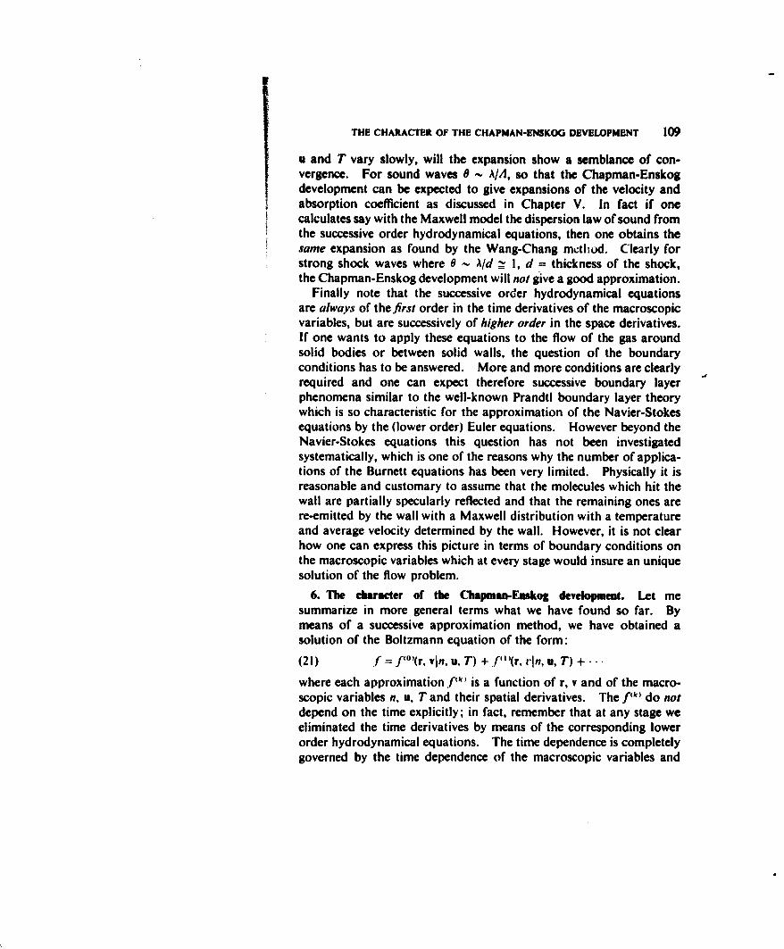
THE CHARACTER OF THE CHAPMAN-ENSKOG DEVELOPMENT 109
u and T vary slowly, will the expansion show a semblance of con-vergence. For sound waves 9 - A/A, so that the Chapman-Enskogdevelopment can be expected to give expansions of the velocity andabsorption coefficient as discussed in Chapter V. In fact if onecalculates say with the Maxwell model the dispersion law of sound fromthe successive order hydrodynamical equations, then one obtains thesame expansion as found by the Wang-Chang methud. Clearly forstrong shock waves where 9 - A/d i 1, d = thickness of the shock,the Chapman-Enskog development will not give a good approximation.
Finally note that the successive order hydrodynamical equationsare always of thefirst order in the time derivatives of the macroscopicvariables, but are successively of higher order in the space derivatives.If one wants to apply these equations to the flow of the gas aroundsolid bodies or between solid walls, the question of the boundaryconditions has to be answered. More and more conditions are clearlyrequired and one can expect therefore successive boundary layerphenomena similar to the well-known Prandtl boundary layer theorywhich is so characteristic for the approximation of the Navier-Stokesequations by the (lower order) Euler equations. However beyond theNavier-Stokes equations this question has not been investigatedsystematically, which is one of the reasons why the number of applica-tions of the Burnett equations has been very limited. Physically it isreasonable and customary to assume that the molecules which hit thewall are partially specularly reflected and that the remaining ones arere-emitted by the wall with a Maxwell distribution with a temperatureand average velocity determined by the wall. However, it is not clearhow one can express this picture in terms of boundary conditions onthe macroscopic variables which at every stage would insure an uniquesolution of the flow problem.
6. The character of the Chapmmn-Enskog development. Let mesummarize in more general terms what we have found so far. Bymeans of a successive approximation method, we have obtained asolution of the Boltzmann equation of the form:
(21) f = f 0'°(r, vin, u, T) + f.')(r, ,In, u, T) +.
where each approximation f.1) is a function of r, v and of the macro-scopic variables n, u, T and their spatial derivatives. The f"k) do notdepend on the time explicitly; in fact, remember that at any stage weeliminated the time derivatives by means of the corresponding lowerorder hydrodynamical equations. The time dependence is completelygoverned by the time dependence of the macroscopic variables and
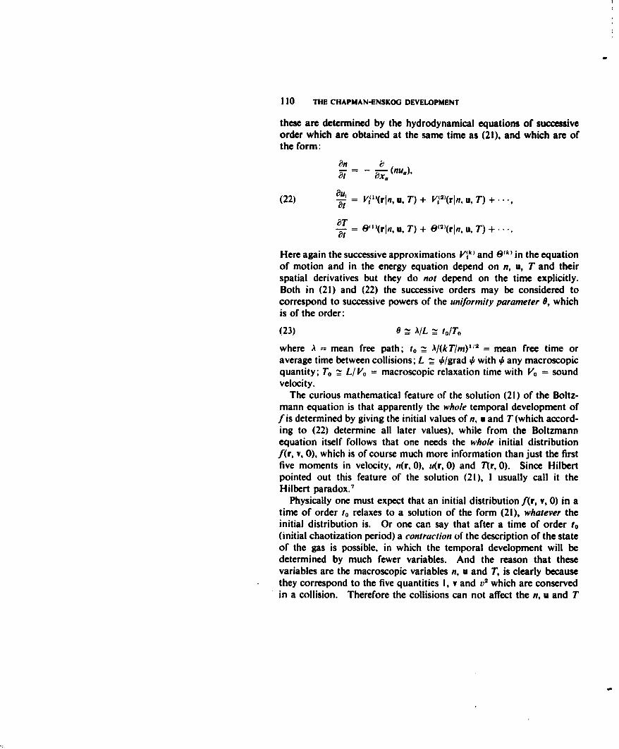
110 THE CHAPMAN-ENSKOG DEVELOPMENT
these are determined by the hydrodynamical equations of successiveorder which are obtained at the same time as (21), and which are ofthe form:
87 =- (nu.),
(22) u., = VV,,(rIn, u, T) + Vi2'(r~n, u, T) +
OT = 1")(rln, u. T) + 8'2)(rln, u, T) +....
Here again the successive approximations V"k) and 1`k) in the equationof motion and in the energy equation depend on n, u, T and theirspatial derivatives but they do not depend on the time explicitly.Both in (21) and (22) the successive orders may be considered tocorrespond to successive powers of the uniformity parameter 0, whichis of the order:
(23) 0 = AlL .t to/T,
where A = mean free path; to L_ AI(kTIm)12 = mean free time oraverage time between collisions; L = #/grad ý with v any macroscopicquantity; To ! LI Vo = macroscopic relaxation time with V0 = soundvelocity.
The curious mathematical feature of the solution (21) of the Boltz-mann equation is that apparently the whole temporal development off is determined by giving the initial values of n, u and T(which accord-ing to (22) determine all later values), while from the Boltzmannequation itself follows that one needs the whole initial distributionf(r, v, 0), which is of course much more information than just the firstfive moments in velocity, n(r, 0), u(r, 0) and 71r, 0). Since Hilbertpointed out this feature of the solution (21), 1 usually call it theHilbert paradox.7
Physically one must expect that an initial distribution f(r, v, 0) in atime of order to relaxes to a solution of the form (21), whatever theinitial distribution is. Or one can say that after a time of order t o(initial chaotization period) a contraction of the description of the stateof the gas is possible, in which the temporal development will bedetermined by much fewer variables. And the reason that thesevariables are the macroscopic variables n, u and T, is clearly becausethey correspond to the five quantities I, v and 02 which are conservedin a collision. Therefore the collisions can not affect the n, u and T
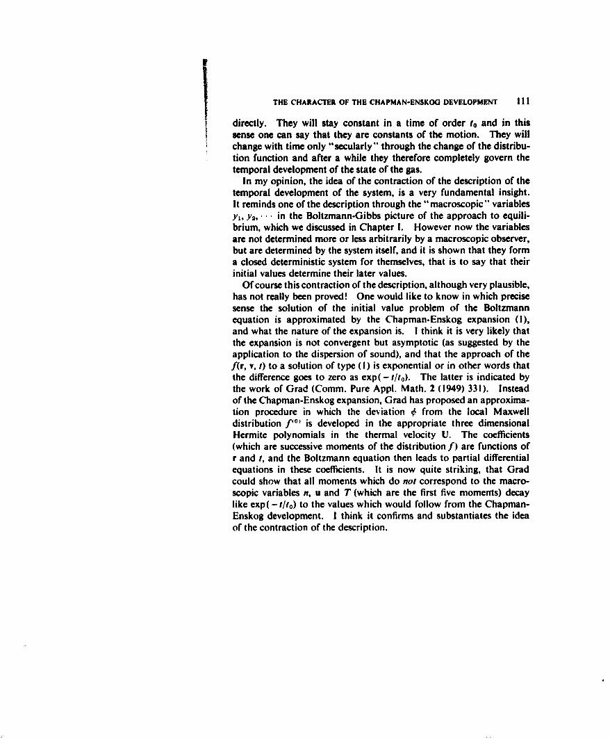
THE CHARACTER OF THE CHAPMAN-ENSKOG DEVELOPMENT IIl
directly. They will stay constant in a time of order t. and in thissense one can say that they are constants of the motion. They willchange with time only ' secularly" through the change of the distribu-tion function and after a while they therefore completely govern thetemporal development of the state of the gas.
In my opinion, the idea of the contraction of the description of thetemporal development of the system, is a very fundamental insight.It reminds one of the description through the "macroscopic" variablesYi, Y2, ' ' ' in the Boltzmann-Gibbs picture of the approach to equili-brium, which we discussed in Chapter 1. However now the variablesare not determined more or less arbitrarily by a macroscopic observer,but are determined by the system itself, and it is shown that they forma closed deterministic system for themselves, that is to say that theirinitial values determine their later values.
Of course this contraction of the description, although very plausible,has not really been proved! One would like to know in which precisesense the solution of the initial value problem of the Boltzmannequation is approximated by the Chapman-Enskog expansion (I),and what the nature of the expansion is. I think it is very likely thatthe expansion is not convergent but asymptotic (as suggested by theapplication to the dispersion of sound), and that the approach of thef(r, v, t) to a solution of type (1) is exponential or in other words thatthe difference goes to zero as exp(- t/to). The latter is indicated bythe work of Grad (Comm. Pure Appl. Math. 2 (1949) 331). Insteadof the Chapman-Enskog expansion, Grad has proposed an approxima-tion procedure in which the deviation 0 from the local Maxwelldistribution f"O) is developed in the appropriate three dimensionalHermite polynomials in the thermal velocity U. The coefficients(which are successive moments of the distribution f) are functions ofr and t, and the Boltzmann equation then leads to partial differentialequations in these coefficients. It is now quite striking, that Gradcould show that all moments which do not correspond to the macro-scopic variables n, u and T (which are the first five moments) decaylike exp( - t/to) to the values which would follow from the Chapman-Enskog development. I think it confirms and substantiates the ideaof the contraction of the description.
NOTES ON CHAPTER VI
1. D. Enskog, Kinetische Theorie der Vorgange in Massig Ver-duinnten Gasen, Dissertation, Uppsala, 1917.
S. Chapman, Philos. Trans. Roy. Soc. London. Ser. A 216 (1916)279; 217 (1917) 115.
The monograph of S. Chapman and T. G. Cowling (The Mathe-matical Theory of Non-uniform Gases, Cambridge University Press,1939; 2nd edition, 1955) follows the method of Enskog. We referto this book for further details. Compare also the treatment of thetheory by L. Waldmann in the Handbuch der Physik, Vol. XII,Section E, p. 384 and in the book of J. 0. Hirschfelder, C. F. Curtissand R. B. Bird (Molecular Theory of Gases and Liquids, John Wileyand Sons, New York, 1954, Chapters 7 and 8).
2. The form of the last equation in (4) is perhaps not quite familiar.Phenomenologically it can be derived as follows. Consider a certainportion of the gas of volume S?, then the work done per second by thesurrounding gas and by the outside forces on the gas inside S2 is:
(a) - ff da P,,u8 + fffdr pa.ugrz. 12
where 1: is the surface of 92 a/nd do, is a surface element with thenormal outwards. Using Gauss' theorem, the equation of motion(Eq. (4b)) and the symmetry of the pressure tensor P1 j, one can trans-form (a) into:
(b) f f f [P.,D., + . Du"JDD
This must be equal to the increase per second of the kinetic andthermal energy of the gas inside .Q plus the kinetic and thermal energywhich flows out of .Q per second. Let e = (1/2)u 2 + (Q/p) be thetotal energy per gram and let s = pfu + q be the total energy fluxdensity. Then one has therefore:
112
NOTES ON CHAER VI 113DuaJI f a( + ffdoas
fffd,,[p.,D., + ,- fffd,(,O)+ f + d,.P.
f fffdl [T(.,) + +u +
f=ff d [p + pu- + ' x0 J
D
fffd (P +
using the continuity equation. Since:
De Dua D IQ\
this gives the integral form of Eq. (4c).
3. Although this is almost self-evident from the way the Eulerequations (7) follow through (4) from the general transport equation(3), one might as well verify it directly. The orthogonality of the leftside of (9) to , 1 = I, leads to:
)fdv/[(0) + f dv r.Iof + af °dv 0.
The last integral is zero and the first two terms clearly give the con-tinuity equation:
On i)(c) + - (nu.) = 0.
The orthogonality condition for v, leads to:
o'- f 'v t!,f( + f dv v,v'f 0° + at dv V, = 0.
Carrying out the integrals, one obtains:
(d) -(nu,) + a (nulu.) + -a k - na, = 0
and this becomes the equation of motion (7b) by using (c) and by
114 THE CHAPMAN-ENSKOG DEVELOPMENT
putting p = nkT. We leave it to the reader to show that the ortho-gonality condition for #s = v2 leads to (7c).
4. By differentiating logarithmically one. gets:
0e o '~t + - + -32 + Mr U( + Va 8+ - - u.) (84- + ,,' au-) - M -a,,(v, -
Now from (7):
(nTl-3 2) = - nT-312),
i1T iýT 2 Tu,-= Uax, - J x.
i'u, iu, I OpW- -= -u 8 •+ a, .-.Pax,
Substituting these expressions for the time derivatives in (e), and using:
it'p = k T +n T
OT 3 2) = T -3 1 - 3 nT- 5,2 OT
i~x1 2 tx
one obtains Eq. (10) of the text, and it is easy to verify that the right-hand side of (10) is orthogonal to 1, U, and U 2 and therefore to the #,.
5. See Chapman and Cowling, I.c. Chapter 10, where one finds
the explicit expressions of 1, and K for various molecular models.For the real Maxwell model u and ,K are proportional to the firstpower of the temperature. That we found for the quasi Maxwellmodel a dependence - T' 2 is clearly due to the artificial assumptionthat the dimensionless function F(O) is independent of the temperature.
6. See again Chapman and Cowling, I.c. Chapters 7, 9 and 10, andfor the Lennard-Jones (6-12) potential, Hirschfelder, Curtiss and Bird,l.c. Chapter 8, §4. The papers of D. Burnett are in the Proc. LondonMath. Soc. 39 (1935) 385 and 40 (1935) 382.
In first approximation for any differential cross-section J(g, 0) one
NOTES ON CHAPTER VI 115
"puts # equal to a linear combination of the same functions #. and002. occurring in the solution for the Maxwell model. Using ordinaryunits this means that one makes the Ansatz:
(f) T = IL u.(cU2 - ý)X +2aD (2UUx-•,U, - -8,.U2)X2
where a = m/2kT, and XI, X2 are constants. This leads to the heatflux density:
2 f •UOq=] 'jdU UUf 0
mn.a )312 1 f dU UU.U2( U2 --aU2
BT
with: 5k V312 ()3/2(g) x --- ,,2 n X1.
Similarly, the second part of the Ansatz (f) leads to the viscositycoefficient:
m-e(,)1 a312(h) P= 2.1,2 n(c)( X2.
Of course, the Ansatz (f) can now only be an approximate solutionof the Enskog integral equation (see Eqs. (9) and (10) of the text):
I Tu.i(aU _ - + 2aD,,(UuU - U -
C(#) = n () f dU, e-U? dQ gi(g, 0)(0' + 01 - -
and in order to determine the Ansatz (f) completely one must still findthe quantities X, and X2. To do this we require that they are the firstdevelopment coefficients in the development in the eigenfunctions0,1. (r = I, 2...) and 0,2. (r = 0, I, 2,.) of the Maxwell model.This leads immediately to:
(i)dUeau2UuUuU2 5
f dU ea UzU - )CUa 2- )
JdU e-a2Ua(UU 80jiU2)(uU.V - 8.U
f fdU ea--3u2 u -U" U, H U" 8"VU2)
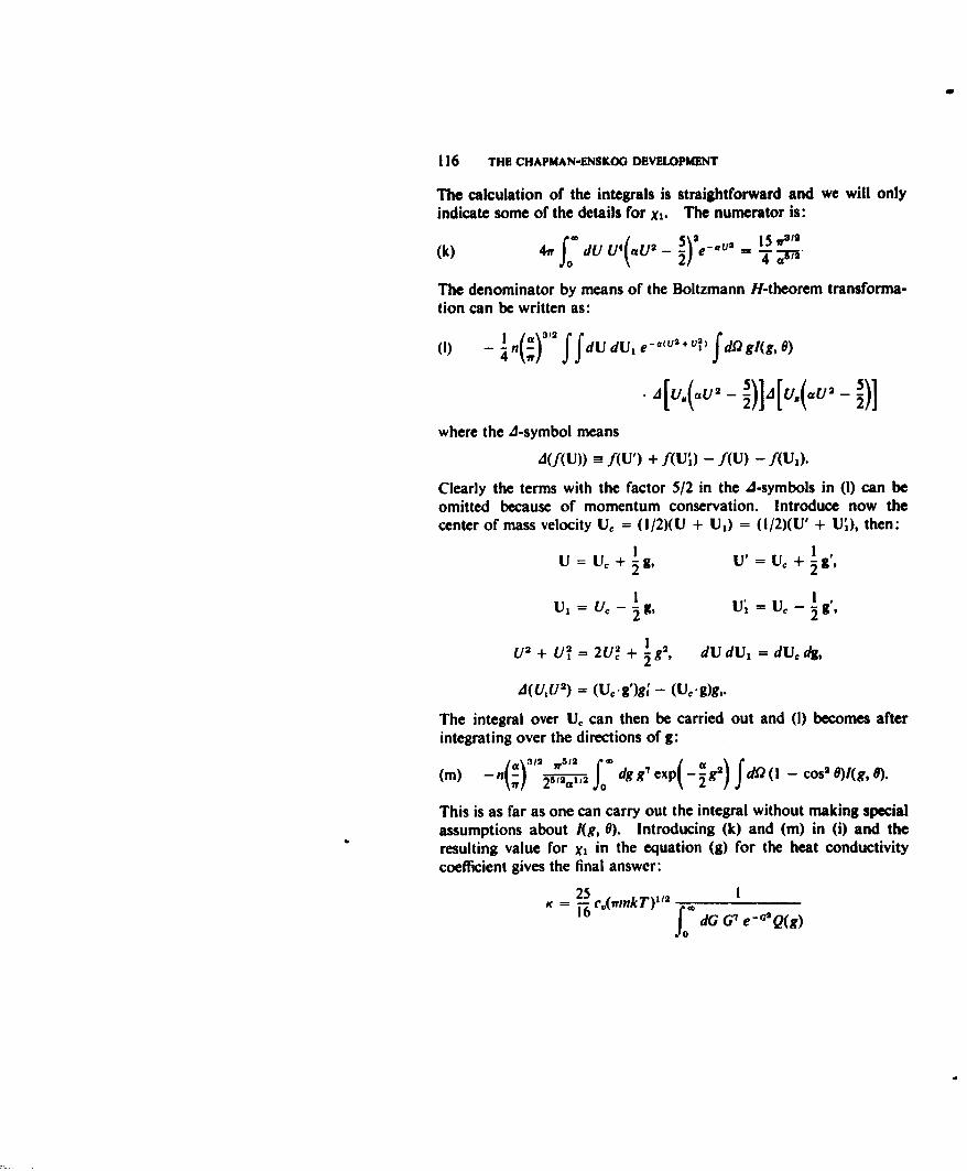
116 THE CHAPMAN-ENSKOG DEVELOPMENT
The calculation of the integrals is straightforward and we will onlyindicate some of the details for Xi. The numerator is:
(k) 4w f dU U4(aU2 - 5 '-,v- 15 _1
-0) 2 a-ST/-2
The denominator by means of the Boltzmann H-theorem transforma-tion can be written as:
(1) ,()32 ffdu dUU e -eg U• f dv2 gl(ge)
J[U.(_U2 _- )l4[u.(au•)]2
where the 4-symbol means
A(f(U)) f(U') + f(U•) - f(U) - f(U1 ).
Clearly the terms with the factor 5/2 in the 4-symbols in (1) can beomitted because of momentum conservation. Introduce now thecenter of mass velocity U, = (1/2)(U + U1) = (1/2)(U' + U'), then:
I 1U U + 2 g, U' UC + 2g'
! IU, Qu - Ig u, U0 - 1g',
U 2 + U2 = 2UIc + Ig, dUdU1 =dUcdg,
4(UU 2) = (U.g')g; - (U,.g)g,.
The integral over Uc can then be carried out and (I) becomes afterintegrating over the directions of g:
(m) -n(a) 3122r! 512 fdgg7 exp(2-"2) fdfl(l - cos2 8)I(g, ,).
This is as far as one can carry out the integral without making specialassumptions about I(g, 0). Introducing (k) and (m) in (i) and theresulting value for X, in the equation (g) for the heat conductivitycoefficient gives the final answer:
25 I_________
K = ? cO(rinkT)1 1 2
1f dG G7 e- Q(g)
NOTES ON CHAPTER Vi 117
where:
c.= G g U
and Q(g) is the so-called transport cross-section:
Q(g) = 2,r fo dO sin' 0 i(g, 0).
The calculation of X2 and hence of u goes along similar lines, and onefinds:
it (-fmk T) 1 12 ®fo dG G7 e -G2 Q(g)
so that the relation (18) of the text remains valid in this approximation.
7. Hilbert in his paper on the kinetic theory of gases (Grundziigeeiner Ailgemeinen Theorie der Linearen Integralgleichungen, TeubnerVerlag, Leipzig, 1912; Chapter 22) speaks of the macroscopic causalitytheorem in this context. In our opinion the word theorem is con-fusing, because macroscopic causality (which means that the state ofthe gas is determined by giving at time t = 0 the density, velocity andtemperature distribution) is clearly a requirement which one imposeson the solution of the Boltzmann equation. The word theoremsuggests also that the macroscopic causality has been proved by theChapman-Enskog development, which is clearly not the case.
CHAPTER VII
The Kinetic Theory of Dense Gases
1. Introduction; the problem of deriving the Boltzmann equation. Therecent development of the kinetic theory of dense systems has startedfrom the question how to derive the Boltzmann equation from thebasic Liouville theorem. Since the subject is still controversial, letme first try to explain why one would want to derive the Boltzmannequation.
It is of course true that the way Boltzmann arrived at his equation,which we presented in Chapter IV, was heuristic and that it thereforeinvites a critical analysis. Historically the criticism of the kineticmethod of Boltzmann was mainly directed toward the H-theoremand was an expression of the feeling of discomfort that somehow usingreversible mechanical models, Boltzmann had succeeded in explainingthe typical irreversible approach to equilibrium. It somehow seemeda swindle! I will not discuss the famous classical objections ofLoschmidt and Zermelo, since they were answered by the statisticalmethod of Boltzmann and the Boltzmann-Gibbs picture which evolvedfrom it. But it leaves completely open the question of how the kineticmethod and especially the Boltzmann equation fits into the generalpicture of the approach to equilibrium.
Besides the logical gap, there are also practical reasons why onewould like to derive the Boltzmann equation. Clearly the applica-bility of the Boltzmann equation is limited to sufficiently dilute gases,so that only binary collisions have to be taken into account. It is therestriction to binary collisions which has as consequence that thetransport coefficients K and it are independent of the density. Qualita-tively this comes about since if only binary collisions are importantthe mean free path A is inversely proportional to the number density(i.e. A - I/na), and, hence, in all transport processes one has an exactcompensation of the number of transporting particles (,- n) and theamount transported by each of them ( - A, hence - I/n) so that theresult is independent of it. If triple and higher order collisions mustbe taken into account, one would expect that:
INTRODUCTION; PROBLEM OF DERIVING THE BOLTZMANN EQUATION 119
(I) A Ino(l + cin + cn'+ -...)
since the number of triple, quadruple -collisions in which a singlegiven particle takes part will clearly be -n 2 , n',.... The compensa-tion of the number of particles transporting and the amount trans-ported by each would no longer be exact, and one would expectvirial expansions for the transport coefficients of the form:
p = Io(T) + p1(T)n + 1,2(T)n2 +..,(2)
K = Ko(T) + Ki(T)n + K2(T)n2 +...
where I0 and K0 are the values given by the Chapman-Enskog theory.In addition one would expect that at higher densities even for mono-atomic gases, the so-called second viscosity coefficient (or bulk vis-cosity) would appear ( n2, I think, since it will depend on the numberof quasi binary molecules). There is considerable experimentalmaterial about the density dependence of K and !, and of the bulkviscosity for dense gases, and at present one is still completely unableto correlate the experiments with theory. In this respect the contrastwith the equilibrium theory of non-ideal gases is quite striking.Clearly the expected expansions (2) are quite similar to the virialexpansion of the equation of state:(3) = I + B(T) + C(T) D(T)
kT1 V 2 V
In fact we saw that B(T) and p 0(T), K0(T) are directly related to eachother since they have to do with only binary interactions. Similarlyone would expect that the third virial coefficient C(T) would be relatedto u,(T) and K,(T), and so on. But, while we know the explicitexpressions for C(T), D(T), • • • in terms of the intermolecular forces,"a similar expression for the transport virial coefficients is not known.
To come back to the Boltzmann equation, it is clear that to develop"a theory for the virial expansion of the transport coefficients one mustgeneralize the Boltzmann equation so as to take into account the tripleand higher collisions. Unfortunately, lacking Boltzmann's intuition,it has (at least till now!) not been evident how one should do this, andhence one has been forced back to see whether one could "derive"the ordinary Boltzmann equation from a more fundamental point ofview, with the hope that this would then also indicate the generaliza-tion to higher densities.
In this chapter I will present the ideas and the method of Bogoliubov.I should say that although these ideas are in my opinion very plausible
120 THE KINETIC THEORY OF DENSE GASES
and although the method has at least the virtue that it gives a definiterecipe how to generalize the Boltzmann equation, it is not so that theyhave led to definite results, which are physically so ev'!ent or whichare so completely in agreement with experiment, that there could notbe any doubt about their validity. As a result the subject is stillcontroversial. Other methods to derive the Boltzmann equation havebeen proposed by Kirkwood and co-workers, by M. S. Green, byPrigogine and co-workers, and by a number of other authors.' Itseems to me that the various methods begin to converge towards eachother and perhaps they will justify the ideas of Bogoliubov. Butfurther clarification is certainly needed!
2. The B-B-G-K-Y hierarchy. Since we do not know how to proceedby intuitive methods, we have to go back to the Liouville equation,which is so to say the basic equation of statistical mechanics. Con-sider again our system of N particles with known interactions in avolume V. The state of the whole gas is described by the probabilitydistribution in r-space DN(XI, X 2 , ', XN,,; 0, where xi - (r,, p)denotes the coordinates and momenta of the ith particle. We takethis distribution to be normalized to unity:
(4) f.. fdxl...dx, DN(xl, '',XN, t)=I
and require, for a gas of identical particles, that DN be a symmetricfunction of xi, x2," ' ", x,. The change of DN with time is governed bythe Liouville equation:
aDN = {-- aIOHN ODN OHaN aDN(5) '-i = JHN Dp, -• -* /_-T t W
with
(6) HNv = ý + U(ri)] + Ir, - rI)
Here U(r,) is the wall potential (no other outside forces will be assumed)and 0( Ir, - r,J) is the interaction potential which is assumed to be ofthe usual van der Waals form discussed in Chapter 1.
Instead of using Poisson brackets as in (5) it is convenient to intro-duce a Hamiltonian operator:
,N(X "... XN) = E . - 2$Im or, O j
(7)0= 01.a + a
THE B-B-wr-K-Y HIERARCHY 121
then (5) can be written:
ODN •N
(8)-
Note that we have omitted the wall potential due to the vessel V, sothat strictly (8) is only valid if the particles are inside V. We willsoon go to the limit N - oo, V - oo, v = V/N finite and then the
effect of the walls will drop out completely so that (8) can be used.From (5) or (8) follows by integration a hierarchy of equations for thepartial distribution functions:
(9) F.(xl, .. ., x.) = V1 f ... f D. dx..,. .dx.
which has been derived by many authors and which I call thereforethe B(ogoliubov)-B(orn)-G(reen)-K(irkwood)-Y(von) hierarchy.' Onefinds:
(10) O-F + X.F, = - dx. + ,+.,F,+1.-If
PROOF. Integrating (8) over x,+x...,XN and multiplying with V%one obtains:
O"+ F. = V3 . d. d {I ... dxx . ,
f .. f -8+1MO,
+ il,, + y i , ,(x, , x,, t).19s;:+1615N 4+1 kc1 J
Since DN must be assumed to vanish for large p, and r, the first andthird terms in the brackets integrate to zero. The second term,because of the symmetry of DN can be written in the form:
V(N - s) •f dx.+, 01., +1 dx.+ 2 .. .dxN
-= -s v Y dx, O+',+ 1F,+ (x', X+V f -~~ . e 1
Hence in the limit N - oo, V -,- oo, v = V/N and s fixed one obtainsthe right-hand side of (10).
122 THE KINEIC THEORY OF DENSE GASES
Since we shall be especially interested in the cases s - I and s - 2,let me write out these cases more explicitly. One gets:
(a) •.-T + E'" F,-• =I
(b) -F + (El. + m P 2. ' ,.2)F2
= I f dxA( 1 3 + 023)FA(x, X2, x 3, 0).
Note that (I la) already smells a bit like the Boltzmann equation.
But of course the connection is still far from clear.
3. The him of Bogollubov. The Liouville equation (5) or the hier-archy (10) to which it is equivalent embodies the mechanical assump-tions. Knowing DN(O) at t = 0, (5) will tell us in principle what DNis at any tat.,: ';.me. 11,,:t how does one know DN(O)? The answeris, I think, th.!,. one i.• n vly interested in those phenomena which areindependent of DN(O), or rather depend only on a few average valuesover DN(O). To see how such a description, essentially independentof DN(O), can come about we have first to look at the basic relaxationtimes. They are:
(a) the time of a collision- rolv., ro = range of the forces (whichfrom now on we will assume to be purely repulsive) and vv is someaverage thermal velocity.
(b) the time between collisions, to = A/z'v; A = mean free path.(c) the macroscopic relaxation time. To = LIVo; L is a macro-
scopic length and Vo is the sound velocity (= i').In the usual situations: slowly varying macroscopic phenomena, not
too dense gases (therefore not for liquids for which ro ! A), one willhave:
(12) - < t0 << TO.
Now Bogoliubov says that one can expect that after an initialchaotization time of order 7-, and for any DN(O) a stage is reached-Bogoliubov calls it the kinetic stage-in which the further temporaldevelopment of the gas is determined completely by the temporalchange of the first distribution function F,(x, t) which in turn isgoverned by an equation of the form:
(13) O-- A(xF)
THE IDEAS OF DOOOLIUDOV 123
where A depends functionally on F, but does not depend on the timeexplicitly. All the higher distribution functions F, depend on thetime only through F, and have therefore the form:
(14) F, = F,(xi,..., xIF1) (s z 2).
To elucidate, note:(a) Eqs. (13) and (14) represent a contraction of the description of
the state of the gas, which is quite analogous to the Chapman-Enskogsolution of the Boltzmann equation which describes the second orhydrodynamical stage of the total relaxation process. Eq. (13) isanalogous to the Ansatz for the hydrodynamical equations (Eq. (22),Chapter VI), and Eq. (14) to the Ansatz for the solution of the Boltz-mann equation (Eq. (21), Chapter VI) which we discussed in theprevious chapter.
(b) Just as in the hydrodynamical stage the contraction is coupledwith an expansion in the uniformity parameter 0 • to/T 9, in thekinetic stage the contraction is coupled with an expansion in powers ofI/v (virial expansion). Bogoliubov puts:
I A~•xF)+I A=(] .(15) A(xIF1) = A(1°(xIF1) + - A"',(xIF1) + A "(XIF)+
C V
and
(16) F. = l.,°(x' .x.IF,) + I ,l"(xl.. .x171) + ...V
Note that the dimensionless parameter in (15) and (16) will of coursebe of order r3/v = ron = r,/A since A - l/nrg. Hence just as in thehydrodynamical stage, the development parameter can be looked uponas the ratio r/to of the two relaxation times in question. However inpractice it is easier to use I/v.
(c) The reason that in the kinetic stage F1 is the basic "secular"variable which governs the temporal development, is because of thefact that the intermolecular forces do not affect F, directly. Only fors >_ 2 does the streaming term XF, contain the intermolecular forceso that F, (s a 2) will change quickly in a time of order r- while the F1will stay constant. In the same sense therefore as in the hydro-dynamical stage and in the time scale to the macroscopic quantitiesp, u and T could be considered constants of the motion, so in thekinetic stage and in the time scale r the F, can be considered to be aconstant of the motion.
(d) The connection with the general Boltzmann-Gibbs picture ofthe approach to equilibrium is I think clear. The contraction is
124 THE KINETIC THEORY OF DENSE GASES
similar to the description through the "macroscopic" variablesYiY2, ,.. except that again the choice of F, is determined by thesystem and not by a macroscopic observer, and that one obtains atthe same time a closed deterministic description through the kineticequation (13).
Of course, all this is a program. We will now proceed to work itout, and then you will see also some of the difficulties.
4. Determination of the functionals F,('). Substituting the virial expan-sion (16) for s = 2 in the first equation of the BBGKY hierarchy (10)one obtains:
O-F, + . = El. (dx e 0 )(X1, x 2 1F1 )
TT m cr1 i'J 2 E1
+ - fdX2 O 1 2 1)(x 1 , x 2 1F I ) +
Hence comparing with the kinetic equation (13) and using the virialexpansion (15) for A(xIF,), one gets:
(17a) A(0)(x IF1 ) = - = - AF1,
(I7b) A'1 '(xIF1 ) = fdx 2 81 2 F1AP(xl, x2 1F,)
and in general:
(17c) A")(x 1jF1 ) = fdx.j 19 2F('- 1 )(x1 , X2 1F)
Since for s > 2, F, depends on time only through its functional depen-dence upon F1 , its time derivative can be expressed in terms of F,through the kinetic equation (13). Indeed, for any functional0(x 1 , X2... IFJ) which depends on time only through F1, a#/at can beexpressed as a new functional of F1 by forming the formal derivative ofý with respect to t and then replacing OF,/&t by A(xlFi) wherever itoccurs in the resulting functional. If in addition we introduce thevirial expansion (15) for A(x IF,), it is clear that one can write:
(18) ý 0(X, X2""..F0) = D10+ I "• o
where the formal operator D") consists in forming the derivative of 0with respect to t and then replacing OF1 /8r wherever it occurs byA(')(xIFi). Of course, the argument x of A" 1(xIF1 ) must be taken as
DETERMINATION OF THE FUNCTIONALs F1,11 125
the argument of OF1 /8t as it occurs in the differentiation process.Hence, substituting the virial expansion (16) for F. into the hierarchy(10) for s > 2 and equating equal powers of I/v one gets:
(19a) D'°)F•°) + g1 F1 °' = 0
and for Il 1:(19b) D),°(F)I + ,F, - D(FI- + fdx,, 9S+ -+1
These equations together with (17) are functional equations for F,()assuming that F, is a given function, which is in principle arbitrary.Presumably (19a) will determine F.(0 ) and therefore especially F2°),which then according to (17b) enables one to find A"). This in turnallows one to find D(I)F,°0 1 and then (19b) for I = I will give F,(1 )which leads to A (2, and so on.
We now have to discuss in which sense the functional equations (19)determine the functionals F,"'. We will assume therefore that theright-hand sides of the equations (19) are known functionals of F, andwe will try to fin(; F.").
The trick Bogoliubov uses to solve a functional equation of theform:
(20) D'°'F,"' + X,.F." = 01.)(xl ... x. IFj)
where OV) is a known functional of F1, is the replacement of the formaloperator D(1) by an ordinary derivative with respect to an auxiliarytime variable 7. To explain this, we introduce the k-particle streamingoperator:
(21) S(xl .. Xk, T) = eXP{('rk(XI... Xk)}.
It is the time displacement operator over the time r due to thestreaming of the k particles in their 6k-dimensional phase space underthe influence of their mutual interactions. If (ri, p) is the phase ofthe ith particle, then in the motion of the k particles the phase ofparticle i a time r later is Sk(r)rl, Sk(7)p,, which is a function of thephases xl... xk of all k particles, although usually we will not putthis in evidence. If x(xi... Xk) is an arbitrary function of the phasesof the k particles then:
(22) Sk(7)X(xl " xk) = x(Sk(')Xl, Sk(')X2 " . Sk(r)xk),
Clearly the Sk(") form an additive Abelian one parameter group of
126 THE KINETIC THEORY OF DENSE GASES
operators; Sk(r.) Sk'2)= Sk(rl + 72); Sk( - 7) is the inverse ofSk(') and Sk(O) = 1. Especially:
(23) S,()x(x, 1) = e' 1x(x, t) x(r + k7,, p,
To replace the formal operator D"0 ' by an ordinary derivative we firstnote that:
" Sl(-r)F1(x, 0) = Xle'•, = XISI(r)F,(24) = _ A(°'(xjS,(r)F,)
using the expression (17a) for A'"). Hence from the definition of theoperator D10 1 it follows that:
(25) Do0 ,,.1F1(x• . xiS1(r)F1 )= - ." F"(x ... x,1S,(,j)F1 ).
Since the function FO(x, 0) in (20) is arbitrary, we can replace it bySl(r)F, and using (25) it follows that (20) is equivalent to the differ-ential equation:
e•F .( x U , . . .x , lS j( i)F j) _ t j ') • (X I . .. X. x S I ( 7)F I)
(26) = -,#V(xl ... x, IS (.r)Fi).
So far nothing has been assumed; one has only transformed (20) into(26) because it is simpler to treat ordinary differential equations thanfunctional differential equations. However in the form (26) one seesthat more information is needed to find the ,". Clearly some sortof initial or boundary condition is required. Bogoliubov assumes thatfor any of the functionals F, for s Ž_ 2:
(27) Lir S,(-7)F.(x .... ,jS,(r)F1 ) = Lim S,(-7) fl Sj(r)F1 (x,, t).
The basic nature of this assumption should be emphasized. What itmeans is most easily seen by considering the spatial uniform case,since then (see Eq. (23)) the SdIa) operator can be omitted and (27)becomes:
Lir S,(- 7)F, = Lim S,(-7) [j F1(p,, I).
We can say therefore that if one traces the s particles back in the pastwhere they will be far apart from each other because of the repulsive
DETERMINATION OF THE FUNCTIONALS F1,11 127
forces, we assume that their momenta are uncorrelated so that the F.is a product of F1 's. This is not obvious! One might for examplejust as well think that the same type of independence would hold forthe future, that is for 7 -, - o. We shall soon see that this is notacceptable since it would lead to a Boltzmann equation for which thedirect and restituting collisions are interchanged so that the H-functionwould increase instead of decrease. It is the boundary condition (27)which selects the appropriate irreversible solutions of the BBGKYhierarchy (10) of the form (13) and (14). The reason why such acondition is necessary while in the corresponding Chapman-Enskogdevelopment there was no need for an analogous condition, is, I think,because the Boltzmann equation is already irreversible while for theLiouville equation (and therefore for the hierarchy) one must choosethe direction of time for which the continuing phase mixing takesplace.'
Accepting the boundary condition (27), let us see how the functionalsF."' can then be determined. First of all from the virial expansion(16) of the F, it follows that (27) implies:
'a) Lim S,(-,r)F0 '(x 1 .. •x, S1(,)F,)
(28) = Lim S,(- 7) S1(i)F1(x,, t),
N Lim S,(-W)T"lx1 ,... .JS,(riF 1) = 0 (1 # 0).
Start from (26) and take first I = 0, in which case the right-hand side#(°) = 0 (see Eq. (19a)). The "solution" of (26) is then:
F.(I(x,' ... x,IS 1(,j)F1) = S,(r)F:0°(x,... xI F,).
Or:
F.°'(0 , ••x,IF,) = S,(-,)F °'0 )(x,.. .x,lS 1(,r)F 1).
The left-hand side is independent of r, so one can go to the limit-r -- (x and from the boundary condition (28a) one then finds:
(29) F,°0 (x. .x, xF0) = Lim S,(-7) 11 S,(r)F,(xi, t).
To find F,") for I > 0 from Eq. (26) one argues in the same way.From the general formal "solution" of (26) one gets:
F'(x, I .. x.I F1) = S.(- r)F,1"(x 1 ... x.IS1(w)F1)
+ f" du, S,( - 7,1)0((xI .• xlS1(?1)F1)
128 THE KINETIC THEORY OF DENSE GASES
and by applying the boundary condition (28b) for? -- o one sees thatthe first term on the right-hand side is zero, so that:
(30) F,"1(x,... x.,IF) = ED dr, S.(-,,)W.,(x,..
Using (29) and (30) the functionals F,') can be determined successivelyfrom the basic equation (19).
5. The kinetic equatioa. Let us now write out according to ourrecipe the first few terms in the kinetic equation. To simplify theformula, let me introduce the abbreviation:
(31) .f,(x1 .. x,) = Lim S(x 1 . .x,, -v) S1 (x,, 7)
since this combination of streaming operators occurs all the time.From (29) one gets:
F2°1(xIx 21F1 ) = .g'2(x 1x2)F1(x1 , t)FA(x2, t).
Hence substituting in (17b), one can write:
(32) A(xuIF) = fdx2 '912YV' 2 F1(x1 , t)F 1(x2, 0)(32)
= ff 4 1 4 2 F1(41. i)FA(2, 0)Q2(X1IC1, W2
with
(33) -Q2(XIC1, 2) = f dx2 292.12' 2(x1 , x2 )8(xl - W)8(x 2 - ,2).
Here C a (4j, wi,) corresponding to x,- (r,, p). Clearly the twolines in (32) are equivalent with the definition (33) for 02. Thereason for writing A")• in the form (32) is in order to separate thedependence on the distribution F, from the mechanics of the binaryinteraction which is embodied in the function Q2.
Turning now to A,421(xIIF,), we have first to find F2(1, which meansaccording to (30) that we have to determine #('). From (29) and thedefinition of the operator D"'), one gets, using the first line of (32)for A '':
D'''F2(0°(xI, X21 FI) = .'1'2jFj(xj, t)A"'(x 21FO + A111(xIF1)Fx(x 2, M)}
= ./'2(1, 2) dxC3 1193/'2(0, 3) + O2 3*/'2 (2, 3))1 F,(x,, t)ifl
DISCUSSION OF THE KINETIC EQUATION 129
where we have omitted the x's in the arguments of the streamingoperators and only indicated the particles involved. Next accordingto (19b) we need F10) which according to (29) is given by:
3
F•°'(x,, x2, x3 1F,) = .Y(1, 2, 3) H F,(x,, t).i-1
Altogether one gets:
012(x 1-, x21F1 ) = dx3 R13 + 923)'Y'3(0, 2, 3)(34)
3
- .3(I. 2){491.W2(I, 3) + 0a3'9"2(2, 3))] 7 FI(x,, t).t-1
Putting this in (30) (taking I = I, s = 2) gives FP2(x 1 , x 21F1 ) and from(17) one then finds A(21. Note that 0,," and therefore also F21) issymmetric in x, x2. Separating as in (32) the distribution functionsF, from the dynamics of the triple interactions, one can finall, write:
3
(35) A121(x, IF,) -- de, d4 3 1 F1(C1 W114(,xu 2, W3)fff t-1
with:
(36) 3(XI 1 , C21 3)3f fo" f= fdx2 0,2 dr S2(I, 2, -r) fdx3 [1 ].I S,(x1,,?)8(x, - •)1=1
where [ ] stands for the expression in square brackets in Eq. (34).1 think this shows sufficiently how the successive approximation
method works, and how one can determine successively the functionalsF.") and A(k). Especially one will get for the kinetic equation:i1F, +pj F, Iff lA fA Iý'W IG ,O I 2I.F1 . d . 2(x1IC1, C2)F'1(C, W)F 1(C2. I)
(37) + Al d, d4 2 d43 Q3(xIC1, C2. C3) I- F,(C,, 1) + ...
which shows explicitly the successive effects of the binary, ternary...interactions.
I will now leave the formal machinery, and will try to discusswhether the results make sense!
6. Discussion of the kinetic equation. There are a number of require-ments which one would expect that the kinetic equation should fulfill.
130 THE KINETIC THEORY OF DENSE GASES
(a) In the first place one would expect that the first term on theright-hand side of (37) is equivalent to the Boltzmann collision term.I will now show, following Bogoliubov, that this is exactly the case forspatially uniform systems.
PROOF. Since in the spatially uniform case F, depends only onp and t one can omit in ./2 the S, operators, and since S2(- 7) actingon pi or P2 only involves the relative coordinate r1 2 = r2 - ri, oneeasily sees from the first line in (32) that A`' becomes:
(38) A()"(pjjF,) =f412 fdr, . ,2F1(Pd2, ,F,(P' 2, t,)
where:
r2) = Lim S2(x1. x2, -4)p, (i = 1, 2)
are the constant initial momenta in the binary collision governed bythe Hamiltonian H2 which leads to the phase xt, x 2 at time zero. The
I2) are functions of pi. P2 and r12. Since in terms of the momentar 2, the Hamiltonian
H2 = Ymm (p• + pI ) + 0,2 = ;I(P,2 )2 + (p22))2}
it follows that:
(39) {H2, F,(P12. t)F1 (P'22 ), t)) = 0.
This is clearly so if H 2 is expressed in the ,), but then it also mustbe so if H 2 is expressed in the original variables xi, x2, since thetransition from x1, x 2 to the p12, is a contact transformation and thePoisson bracket is invariant under such transformations. Writtenout in the variables xi, x2, Eq. (39) implies:
0 1 2FW(P'12, I)FI(P''2 , ) = P2 - P, 2 F1 (P32 , /)Ft(P('22 , t).m •~1
Putting this in (38), and using in the r12-integral cylindrical coordinateswith the axis in the direction of the relative velocity g = (P2 - p)m,
Eq. (38) becomes:
(40) Al'"(plIF1 ) = dp2 , gb dbedf_ dl Fi(P?), t)FI(P2), t)
where I is the coordinate along the cylindrical axis and (b, e) are thepolar coordinates perpendicular to this axis. Clearly the /-integralcan be performed. Since at I co - the two particles are outside
DISCUSSION OF THE KINETIC EQUATION 131
their action sphere and since the S2( - ) will never bring them to-gether:
Lim P•2)=p. (i= 1,2).I- - O
On the other hand for I -* + x, although the particles are then alsooutside their range of interaction, the S2(x1 , x2, - 7) operation for7 -- oo will certainly produce a collision and therefore:
Lim p 2 1=pp, (i-- 1,2)1- + W
where the pi are the momenta of the restituting collision (pi, p2) -,
(PI, P2). Introducing again the differential cross-section I(g, 9) by:
b db d. = I(g, O) dQ
(40) becomes:
A" 1(p IF1 ) = f dP2 fdQg1(g, 0)[I,(pl, I)F,(p2. 1) - F1(p, ,F 1(p2, 01
which is the Boltzmann collision operator.For systems which are not spatially uniform the proof breaks down
and in this case the Boltzmann form of the collision operator can onlybe an approximation of the A"1 1(xIFI). In a sense this is satisfactorysince in the intuitive derivation of the Boltzmann equation it is clearthat some uniformity assumptions were really implied. For instancethe difference in position of the colliding particles was neglected andit was assumed that the changes of F, in time due to the streamingand due to the collisions are strictly additive and do not influenceeach other. Clearly both these assumptions can only be valid if thespatial variation of F, is small, and it is therefore satisfactory that theBogoliubov theory gives a more general form of the binary collisionoperator.
(b) The collision terms A"), A'2)... must have the cluster-property,which means that they must be zero if the particles do not- make abinary, triple .. collision. For A"() this is obvious, because if thetwo particles stay outside their action sphere then the operator 912
will make 92 and therefore A1̀ ) zero (see Eq. (33)). For AM2 ) it canbe verified as follows. From Eq. (36) for -Q3 one sees that the inte-grand of the x2-integral will vanish if Jr 2 - ril > ro because of the912 operator. Consequently one needs to consider only those x2 forwhich Ir2 - r,1 < ro. For this phase (x1, x2) the S2(0, 2, -r) opera-tor separates the particles I and 2 by a distance r. in a time of the
132 THE KINETIC THEORY OF DENSE GASES
order of the collision time and from that time on the distance of theparticles increases. Put:
2, = S2(l, 2, -,v)x,, (i = 1, 2)
and call 7' the time for which the distance Ir2 - r, has become largerthan 2ro. The operator occurring in the v-integral in (36) can nowbe written as:
f dx3 [{101, X3) + 123(Q2, X3)}.)' 3(91 , 92, X3)
(41)- .5 2(Q1, 92 ){ 0
1 3(-tl, x3 ).¶/'2(21, x3) + 023Q21 x 3)9 2(2 2, x3)}].
For 7 > 7', 012(2•, )?2) = 0 and for fixed x 3 either 913(01, x3) or923(R2, x3) must be zero, since R1 and 92 are separated by a distancebigger than 2r0. Suppose 813(91, x3) = 0, but 023(92, x 3) 6 0.From the definition of .93, and since for this configuration X 3 =X 2(72, x3) + "(x 1), it is clear that one then has:
Y013(21, g 2, x3) = ./ 2(! 2. x 3)
and since in this case .Y0'(1, -i2) = I one sees that the operator (41)goes to zero. This is also the case if 602 0 2, x3 ) = 0 but 13(.01, x 3) :0 0by a similar argument, and hence one can conclude that Q 3 is onlydifferent from zero if for a time of the order of the collision time thethree particles are in a connected configuration.
It would be very valuable if one could further "understand" theexpression for 'Q3, in the same way as one "understands" the Boltz-mann form of the binary collision operator. For instance one mighthope that in the spatially uniform case one could transform A3 in asimilar way as Q2, so that one would see that . 3 depends only on themomenta of the three particles before and after the triple collision.We have not succeeded in doing this and I doubt whether it is possible.However, I still think that it should be possible to see so clearly throughthe structure of the successive collision kernels .?2, -3 ... that onecould imagine that with enough insight one would have written themdown intuitively just as Boltzmann wrote down his collision term.
(c) One should expect that the kinetic equation will lead to thestate of thermodynamic equilibrium and that then F1 and all thehigher distribution functions will agree with the results obtained fromthe canonical ensemble. It is rather easy to verify that if one takesfor F, the Maxwell distribution:
(42) Feq(x) = (21rmkT)- 312 e- p2 2mkT
DISCUSSION OF THE KINETIC EQUATION 133
all the functionals A")(xjFjq) vanish and that then the functionalsF,(xl... xFl") become the successive terms in the virial expansionof the s-particle equilibrium distribution functions. The simplest isto prove this successively and after a few orders it will then be clearhow it goes on.
In zeroth order with (42) A101 is obviously zero and since Ffq isspatially uniform one obtains from Eq. (29):
F.°)(x,. x. Ix lF0) = (2,rmkT)-- h2exp{ 2 , k
where:I') = Lim S.(-7)p,
are the momenta of the s particles before the s-tuple collision. Sincethe Hamiltonian for the s particles can be written as:
Hs = + . = (
one can also write:
(43) F(,°'(x, •. .IFj'q) = (21rmk T)- 3'12 e- H. kT
which is the expected form for the s-particle distribution function atvery low density.
In first order one obtains from (43) and (17b):
A (1(x, IF'lq) (21rmkT) -I fdX2 192 exp( pA + P22 0_12a•fk ( 2mkT UkT)
Introducing the relative coordinate r = r 2 - r, the space part of thex2-integral will be:
f rL - #kTOre
which is clearly zero. Hence A(1)(xjFj1 q) = 0 as follows of coursealso from the Boltzmann form for A"). Since A") = 0, D(1 )F,°0 ) = 0,and since from (19b) and the definition of 0,•') in (20), restrictingourselves to the case s = 2, one has:
OI(x 1 , x2IF,) = -D("'FJ° + fdx3(013 + 023)F•0 )
134 THE KINETIC THEORY OF DENSE GASES
one obtains from (30) and (43):
(44) FN1)(xI, x21FIq) = (2wmkT)-s' 2 f dr S2(, 2, -,r)
x dx3 (913 + 9 23 ) e"-'3kT.f
From {H3 , exp( - H3 /k T)) = 0 follows:E. P2 D e, 2 e-HakT + e - U.
(M13 W1 )W-"S2 m )m M mWa3
Introducing this in (44) the last term clearly integrates to zero. Since:
S 2(l, 2, -7) E a +P2 m _-- 12
= S2(l, 2, -7))r 2
= X.SA(l, 2, -) - S 2(, 2, -)
the T-integral in (44) gives:
PI - S2(, 2, - oo)]e- H3k T .
Writing H, = H2 + p3/2m + 01, + #23 and integrating over P3 , onegets:
F2"'(x,, X21F~q)
= (2vmkT)[- '[ - S2(0, 2, - 00)]e-H2'kT. fdr3 e-(03+a IkT.
Introducing the Mayer function f, = exp(-0j,/kT) - I, one canwrite:
f d,3eXp[-(0,3 + 23)IkT] = fdr3 (fia.f 2 3 +Af3 +f23 + 1).
The last three terms are constants, independent of (xI, x2 ), so that[I - S2(0, 2, - cc)) acting on them will give zero. The first term is afunction of Ir2 - r,1, which is zero if jr 2 - r,1 > 2ro, so that:
S2(l, 2, -c) fcl.f,3.f = 0.
One obtains therefore:
F2"(x1 , x2 lFtX ) = (2vmkT)- 3 e- H2kT f dr3af 3f2a
F21°)(x,, X21F1*q) f dr•.fl3f23
REMARKS ON THE THEORY OF THE HYDRODYNAMICAL STAGE 135
which is the familiar expression as derived from the canonical distribu-tion." By the same argument as used for Al'1 it follows from (45)and (17c) that A' 2)(xaIFP) = 0, and so on!
(d) We have shown therefore that the equilibrium distributionsare solutions of the Bogoliubov equations. Are these solutions alwaysreached in time? Or in other words, can one generalize Boltzmann'sH-theorem? Unfortunately there is here a gap in the theory. So farwe have been unable to do this. I feel sure that it must be possiblebut one is hampered by the lack of insight in the structure of thesuccessive collision kernels so that it is difficult to see how one shouldgeneralize the argument of Boltzmann.
7. Remarks on the theory of the hydrodynamical stage. It would takemuch too long to explain in detail the further work of Dr. S. T. Chohon the generalization of the Chapman-Enskog development to thekinetic equation of Bogoliubov. Let me therefore only point outwhat is involved and indicate how far the theory has progressed.
The first step is again the derivation of the general macroscopicequations. Since these equations are exact consequences of theBBGKY hierarchy, and since it may be useful to have them somewheretogether I will still write them out in detail, and to facilitate the com-parison with the analogous development in §2 of Chapter V! I willuse in parallel with F,, F2, ..- the distribution functions f,(r, v, t),f 2(r1, r2, v,, v2, 1) in the velocities instead of in the momenta. Theconnection between them is given by:
Nf,(r, v, t) dv = P F0, p. t) dp,
( (r4, r 2, V , , V ) d v 1 d v 2 = N ( N - I) F 2(r) , r P 1, P 2 , 1) 4 11 d P 2rf (r(r r r , P , P ,)t) dpd dp=
and so on.The macroscopic quantities, which describe the macroscopic state
of the gas, are:(a) the mass density p = nm, where:
n(r, 1) = f dvrf,(r, v, t);
(b) the average flow velocity u(r, t), defined by:
nul(r, 1) = fdv vf[(r, v, t):
136 THE KINETIC THEORY OF DENSE GASES
(c) the internal energy density e(r, t), which consists of two parts:
(47) t(r, t) - ek'n(r, t) + ei`t(r, t)
where:
(47a) = m f dv U2fl(r, v, t)
with U, = v, - u, = thermal velocity (note that Ekta was called Q inChapter VI), and where:
(47b) =pot __ f dv fdvr fdr1,4(Ir - r1 l)f2(r, r1, v, vi, t).
In terms of these five quantities one obtains from the BBGKYhierarchy the macroscopic equations in exactly the same form as inChapter VI, namely:
(a) e+ (pUa) 0,
(48) (b) Du, O pt,.
(c) P + = - PaD.,
with:
D e, i 'U u)Tt = Ft + UT-.
However now the pressure tensor Ptj and the heat current density qiconsist just as the energy density - out of two parts, a kinetic partand a part which depends on the intermolecular potential #. Onefinds:
(49) P 1, = " + Pr t
where P,'" is defined just as in Chapter VI by:
(49a) Pt"(r, t) = m fdv UUJf1 (r, v, t)
and where:If pep, d# P•
(49b) PI t(r, V ) = - dp dP'' d• J dA n2 (r1 , r., t).
REMARKS ON THE THEORY OF THE HYDRODYNAMICAL STAGE 137
SHere n2(r1, r2, 0) is the pair density distribution defined by:
• (50) n2(rf, r2, t) dv1 dv2f 2(r1 , r2, V1, v2, t)
and the positions r, r2 are related to r, and the relative coordinatep - r2 - r, by:
(51) r, = r + (A p)e, r2 = r + .p p
Finally one has:
(52) q,= qd + qr"
where again q'1 is defined just as in Chapter VI by:,I(52a) qk'n(r, t) = m f dv U, U 2f,(r, v. t)
and where:
qrO(rt) f dri. dv dvf U1,.(Ir - r,1 )f 2(r, r1 . v, vit)
+ Ib dp 1 L f- dAff d,1 d 2(Ul.. + U2.Jf 2(r 1 , r2, v,, V, 0).
4 Jfp 2 dp Jo J
In the second line the positions r,, r2 are again expressed in r and pby (51), and
U, = - u, (i = 1,2).
In note 5 we indicate some of the rather straightforward manipulationsrequired to derive (48) from the BBGKY equations. It is also notdifficult to give a physical interpretation of the potential energy partsin P,, and q,, but we will leave this to the reader.
One now has to use the expressions the Bogoliubov theory gives forthe second distribution function F2 in terms of Fi, and then just as inEq. (21) of Chapter VI one must develop F, in an uniformity para-meter 0, postulating at the same time hydrodynamical equations ofthe form:
bnFt = ON " t) + O2N '2 . .
(53) OU_ = oV,1 + 02V,(2) +
at
T = OEV) + 02E'21 +...
138 THE KINETIC THEORY OF DENSE GASES
where the N"11, V11 and El'• are functions of the position r and dependon the time only through their functional dependence on the macro-scopic variables n, u and e.
Unfortunately the formulas become rather involved, and for alldetails I have to refer to the dissertation of Dr. S. T. Choh. In con-clusion let me therefore only state what Dr. Choh has been able toshow.
I. In first order of 0 one gets the ideal or Euler hydrodynamicalequations, in which the pressure p as function of T and p is given bythe usual (equilibrium) virial expansion and where the internal energyz is given by the corresponding thermal equation of state.
2. In second order of 0 one gets the Navier-Stokes equations, orin other words one obtains Fourier's law of heat conduction:
OTq, = -- K Tx-1
and Newton's law of internal friction:
Ply= p•, - 2, 1(D,, - I 8j 1Da) -
which now involves two viscosity coefficients.3. For the transport coefficients gA, JA2 and K one gets virial expan-
sions of the expected form (2), but unfortunately the actual values ofthe expansion coefficients depend on the solution of inhomogeneousintegral equations of the same form as occur in the Chapman-Enskogtheory but much more complicated since the inhomogeneous part nowinvolves the three particle streaming operator. One can show thatthese equations have an unique solution, but to find the solution evenfor special intermolecular potentials (like the elastic sphere or theMaxwell model) seems very complicated, so that no numerical resultshave been obtained so far.
NOTES ON CHAPTER VII
1. The work of N. N. Bogoliubov was published in his book:Problemy Dinamicheskoi Teorii v Statisticheskoi Fisike (Moscow,1946). An excerpt in English appeared in J. Phys. (U.S.S.R.) 10(1946) 265, and a complete translation (by E. K. Gora) appears inthe first volume of the "Studies in Statistical Mechanics" (NorthHolland Publishing Co., Amsterdam, 1962). A short account of thetheory was presented by one of us at the Boulder Summer Seminar in1957 and this was published as Appendix I in the book by M. Kac(Probability and Related Topics in the Physical Sciences, Interscience,New York, 1958). Further consequences of the Bogoliubov theoryhave been worked out in the University of Michigan dissertations ofS. T. Choh (The Kinetic Theory of Phenomena in Dense Gases, 1958)and of R. L. Guernsey (The Kinetic Theory of Fully Ionized Gases,1960). In the text we follow mainly the exposition by S. T. Choh.
The work of J. G. Kirkwood has appeared in a series of papers inJ. Chem. Phys. See especially: J. Chem. Phys. 14 (1946) 180 and 15(1947) 72. Compare also the account given by J. G. Kirkwood andJ. Ross in the Proceedings of the International Symposium on Trans-port Processes in Statistical Mechanics (lnterscience, New York, 1958).In these proceedings one also finds a paper by M. S. Green, which is asummary of his article in the J. Chem. Phys. 25 (1956) 836. Morerecent work of the same author appeared in Physica 24 (1958) 393 andin Vol. III of the 1960 Boulder Lectures in Theoretical Physics (Inter-science, New York, 1961).
The work of Prigogine and co-workers appeared in a series ofpapers in Physica since 1956. Some of the recent ones are by I.Prigogine and R. Balescu, Physica 25 (1959) 281, 302, 324; 26 (1960)145, 529. Compare also the application to the kinetic theory ofplasmas by R. Balescu (Phys. Fluids 3 (1960) 52).
A useful comparison of the different methods of deriving theBoltzmann equation has been made by E. G. D. Cohen (Physica 27(1961) 163). In here one finds also further references.
Finally one should point out that thefirst attempt of a kinetic theoryof dense gases was made by D. Enskog (Kungl. Svenska Vet. Akad.Handl. 63, No. 4 (1921); see also Chapman and Cowling, Mathematical
139
140 THE KINETIC THEORY OF DENSE GASES
Theory of Non-uniform Gases, Chapter 16). Enskog always used thehard sphere model and he started from the Boltzmann equation inwhich the collision term was modified by taking into account thedifference of position of the two colliding molecules at the moment ofimpact and by assuming that the influence of the other molecules canbe accounted for by changing the collision probability by a factor
(a) x= 5b
where b is the van der Waals' b, which insures that in equilibrium theequation of state is correct up to and including the third virial co-efficient. To this modified Boltzmann equation the Chapman-Enskog development can be applied and this leads to a virial expansionof the transport coefficients of the form (2). In fact one finds:
_ + 7b,0 +"40 +
(b)K = 23 b+..
+~ - +K0
40 V
The Enskog theory has been discussed by many authors; see forinstance: H. B. Hollinger and C. F. Curtiss, J. Chem. Phys. 33 (1960)1386 and J. V. Sengers and E. G. D. Cohen, Physica 27 (1961) 230,where one finds also further references. There is no doubt that theEnskog theory explains at least qualitatively what happens at higherdensities. However, because of the lack of a systematic procedureand especially because of the uncertain validity of the Ansatz (a), it isat present not known whether the numerical coefficients in the virialexpansions (b) are correct.
2. For the derivations by Bogoliubov and by Kirkwood see thereferences in Note I. The work of M. Born and H. S. Green appearedin a series of papers in the Proceedings of the Royal Society. They arecollected in a book called A General Kinetic Theory of Fluids (Cam-bridge University Press, Cambridge, 1949). For the work of J. Yvonsee his monograph La Theorie Statistiques des Fluids in the Actualit~sScientifiques et Industrielles (Hermann, Paris, no. 203, 1935).
3. The fact that the application of a boundary condition like (26)but for r -* - co leads to the wrong sign in the collision term of theBoltzmann equation, was pointed out by E. G. D. Cohen and T. H.Berlin (Physica 26 (1960) 717). In this paper and also in the article
NOTES ON CHAPTER V11 141
by E. G. D. Cohen (Physica 27 (1961) 163) it was pointed out that inall derivations of the Boltzmann equation from the Liouville equationa similar choice of the appropriate solution is made.
Clearly a further clarification of the role of the boundary condition(26) can come about only when one sees in which way the solution ofthe initial value problem for the Liouville equation reaches the form(14) postulated by Bogoliubov. We hope and we expect that thisinsight will come from the work of M. S. Green.
4. See J. E. Mayer and E. Montroll, J. Chem. Phys. 9 (1941) 2,where one finds the general expressions for the F,')(xl... x,IFt").For a discussion of the virial expansion of the s-particle distributionfunction with the help of the theory of linear graphs as in Chapter IIsee the review article of the authors quoted in Note 6 of Chapter II.
5. We will follow essentially the work of J. H. Irving and J. G.Kirkwood, J. Chem. Phys. 18 (1950) 817. The method is completelyanalogous to the method used in Chapter VI to derive the macro-scopic equations from the Boltzmann equation.
Start from the first equation (I la) of the BBGKY hierarchy.Integrating over Pi leads immediately to the continuity equation (48a)since the right-hand side vanishes. Multiplying (I la) by p1/m andintegrating over pl, one obtains after some simple transformations:
(c) p "-Dui -x drJdv dv 1dirr-- )f2(r, r,, V, V1, t)
where we have changed to velocity variables and the distribution f2according to (46). The question remains to show that the last termin (c) can be written as the divergence of the second part Pf' of thepressure tensor. The simplest way is to verify. From (49b) one gets:
- f2 dp P f dA n2(r1, r2, 0).
Since n2 is a function of r + Ap/p and p (see Eq. (51) defining r, andr2), it is clear that:
OA PO x.
Hence:- 2dp' d {n 2(r, r + p, t) - n2(r - P, r, t)).
142 THE KINETIC THEORY OF DENSE GASES
Changing in the second term the direction of p, and using the sym-metry of n2 in the position variables, one gets:
"•pr. f dpL,do n2(r, r + p, )Ox. - p dp- P ,
and this is identical with the last term in (c) if there one puts r, =r + p.
To derive the energy equation (48c) one multiplies (I la) by p'/2mand integrates over pl. Using (48b) one then obtains:
) + +k-- = -Pa#Do +a (u0P:
(d ) - r d r , T x
d r - ri)Af2(r, r1, v, v1, t).
To obtain the transport equation of the potential energy density wehave to use the second equation (I1 b) of the BBGKY hierarchy. Bymultiplying (I Ib) with 0( ]r, - r 2 /)/2 and by integrating over r2, piand P2 one obtains after some rearrangements and renamings and afterchanging to velocity variables:
D ( + =t--)
(e) 0 r - if -2! fd, ffdvd,,(,o- ,) °)#( Ir - r ,l)f( r,, v, v,, t)
where q01 ' is the first part of the potential energy part of the heatcurrent density given by the first line in Eq. (52b). Adding equations(d) and (e), and using the expression (49b) for Pt1, one gets:
p D (•) + jq k +q•,,,,)= _paDaR
fdr, ffdv d., r-1) (U. + U1.)f 2(r, r1, v, vj, t).
Finally it is easy to verify that the last term is the divergence of thesecond part of qI,*' given by the second line in Eq. (52b), which con-cludes the proof of the energy equation.
APPENDIX
Quantum Statistics of InteractingParticles
By ELLIorr W. MONTROLL
I. The plrtition functio. As was pointed out in the lectures ofProfessor Uhlenbeck, the calculation of thermodynamic properties ofan assembly of particles can be accomplished by performing appro-priate elementary operations (taking logarithms, differentiation, etc.)on the partition function. In the case of an assembly whose dynamicsis described by the laws of quantum mechanics, this function is
(I) Z= exp- PE,j
where the set {E,) is the set of all energy levels of the assembly; i.e.the set of characteristic values of the Schrddinger equation
(2) H#, = Eo,,
the H being the Hamiltonian operator of the assembly and the Oy'sthe wave functions or characteristic functions of H. The parameterP is I/ iT, T being the temperature of the assembly and k Boltzmann'sconstant.
Clearly, if one can solve the Schr6dinger equation for the assemblyof interest, the calculation of Z is trivial. Generally, 0 is a functionof 3N (with N = 0 (1023) being the number of particles in our assembly)variables, say the position vectors of the particles in the assembly, andH is an operator which depends on the same variables. If onepostulates additivity of intermolecular forces, then
(3a) H = I " + I I rjk)2 I1 k>J I-=
wherea2 jý2 e2
(3b)4 XI y12yj+ T143
144 QUANTUM STATISTICS OF INTERACTING PARTICLES
and 0(r") is the potential energy of interaction between the ith andjth particles when they are separated by a distance r". The onlyinteresting case of interacting particles for which the Schrbdingerequation has been solved exactly is that of coupled harmonic oscillators(crystals undergoing small vibrations). For all other significantexamples, approximations must be made. My lectures are concernedwith the systematic application of perturbation theory to the problemof the calculation of the partition function. Although a considerablepart of the discussion will be quite general, the example which I hopeto analyze in some detail is that of the gas of ionized particles. Inthat case 0 represents the coulomb interaction
eije
(4) 4(rI') =
ej being the charge on the jth particle.The methods presented in the lectures are those developed by J. C.
Ward and myself. They are closely connected with those developedindependently by Matsubara; Huang, Lee, and Yang; Bloch andDiDominicis; Gell-Mann and Brueckner; Goldstone, and otherauthors. The characteristic feature of all this work is that perturba-tion theory is developed in a systematic way and that diagrams areused extensively. These techniques were inspired by the celebratedpaper of Feynman on the theory of electrons and positrons. As thedevelopment proceeds, I suspect that occasionally you mathematicianswill be amused by the methods, but probably the recklessness of theapproach will more often give you a feeling of uneasiness. A propermathematical investigation of the expansion of the partition functioninto a series of divergent cluster integrals and their recollection intoconvergent expressions would be most welcome.
Actually, Martin and Schwinger, Fradkin, Siegert and others havediscussed the partition function by nonperturbative techniques butthese lead to the necessity of making other types of approximation.Their approach will not be discussed here but it might be of interestto some of you.
The partition function (I) can be written in an alternative form interms of the characteristic functions {#,} of (2). Each € depends onthe schematic variable(5) r {r 1, r 2, r..,rN}.
Then
(6) Z J .f. f 4)0*(r)O)(r)e-"i d3Nr = trace exp - PH.
THE PARTITION FUNCTION 145
Note that the operator exp -PH plays a decisive role in equilibriumstatistical mechanics while exp itHN/ is the operator from whichdynamics can be developed. That is, the real part of the complexvariable P + ith-i is associated with thermodynamics and the imagin-ary part with dynamics while both the real and imaginary parts findtheir place in the statistical mechanics of nonequilibrium processes.We start our development with an analyses of Boltzmann statistics.In the case of fermions or bosons the summation over j in (6) and (7)is taken over only antisymmetric or symmetric #'s.
We define what is technically known as a "propagator"- by
K(2, 1) _=K(r2fi2; r1fli) = ~feAD)s~~l.j 2) if P2 ?- P1
(7) 0 ifP2i < P1
= 00(f2 - 9i1) • e-(0a - 0 d10, *(rj)0Ar2 )
O(x) being the Heaviside step function
(8) O(x) = Iif X < 0
(9) dO/dx = 8(x).
The partition function is then
(10) Z= fr... f Krfl; rO)d 3 r.J V
Although the case #2 < P, does not appear directly in this formula,the setting of K - 0 under this condition will be convenient in theperturbation theory of the calculation of Z since certain restrictedintegrations over P's will be replaced by unrestricted ones. Actually,an extra factor I/N! should be introduced into (10) because in inte-grating freely over the r's, many sets of possible positions differ fromeach other only through a permutation of particles so that they areovercounted by a factor N!. In §§ I and 2 lower indices on r'sidentify the value of P with which the r is associated; i.e. r2 is ther value (Eq. 5) at fl. The upper indices denote particle numbers.
Since
(II) 0'*(r)0#,(r2) = 8(r2 - ri),
(12) H(2),,(r2) = E,0#,(r 2), and i)8(x)/1)x = 8(x)
146 QUANTUM STATISTICS OF INTERACTING PARTICLES
where H(2) is the Hamiltonian operator in terms of the variables
(13) r2 = {ri, r2,. •., r'},
we have
(14) + H(2) K(2, I) = S(2 - Pi)8(r2 - r,).
This equation is just the Green's function form of the Schr6dingerequation with P replaced by it/h. The .homogeneous form of thisequation is often called the Bloch equation. The propagator is aGreen's function.
In the case of free particles, the Hamiltonian is
(15) HO(2) h-2 V2/2m
and (14) is just the point source diffusion equation for N independentparticles with a diffusion constant D = h2/2m. In all cases
NWr2 - r,) = II - r').
= 1
The free particle propagator, which is the solution of
(16) + +lo(2) Ko(2, I) = W(/i2 - PO) 8(r 2 - r,),
is thenN
(17) Ko(2, I) = OA - P,) F1 Ko1(2, I)J-1
where K1(2, I) has two equivalent forms in the case of an unboundedspace
(18) Kol(2, I) = f exp ip'.(r' - r1)h(21rh)3 f2 1
2m- •2 d3p'
(19) _- exp - {m(r1 - rl)2/2h2( 2 -2 )
[2,rh'(P2 - Pl )/m]3/2
The form for K/1 in a finite cubic box of volume L3 = V with periodicboundary conditions is(20) V (
e(2pI)3 Lr/ (- )2×exp [i(pý.rl - pIrA)/lh - Ap - ,XpJp/2M]
PERTURBATION THEORY 147t where the summation proceeds over all momentum states
(21) 2wnh(21) P='T'-h n = 0. , + ±,2,..
and 8,.P ,P is a Kronecker delta. As L - oo we write
(22) d3p = (21rh/L) 3
so that the summation becomes a double integral. The fact that
(23) 8(P2 - P1) lim Vh)3v-. (2wrh)
implies that (20) reduces to (18) in the required limit.
2. Perturbation theory. With a knowledge of Ko, we are preparedto give a systematic perturbation theory of K. Let
H1= Ho + H,
where H. is given by (15). Then the differential equation (14) isequivalent to the integral equation
(24) K(2, 1) = Ko(2. 1) - f f Ko(2,3)H,(3)K(3. )d 3Nrd 3d.
This equivalence can be verified by applying the operator (/•'/ 2 + H(2))to obtain (in view of (16) and (24))
T-4+ H(2) K(2, I) = I1,(2)Ko(2, 1) + W4,82 - /S) (r2 - ri)
-Hi(2)f f Ko(2, 3)H,(3)K(2, 1)d3 Nr 3
- fv f (4 - #3) (r2 - r3)
x HI(3)K(3, 1) d Nr3 dfA3
= Ht(2)Ko(2, 1) + 8(f• 2 - /%) 8(r2 - r1)
- H,(2)K(2, I) + H,(2)[K(2, 1) - Ko(2, I)]
= fl2 - 1) 8(r2 - ri)
as is required. Since both Ko(2, 1) and K(2, I) were defined to vanishwhen fl < #,, the limits on (24) could just as well be written as goingfrom #I to / 2 so that (24) is equivalent to
(25) K(2, I) = Ko(2, 1) - f f 2 Ko(2, 3)H,(3)K(3, 1) d 3 r3 dl3 .
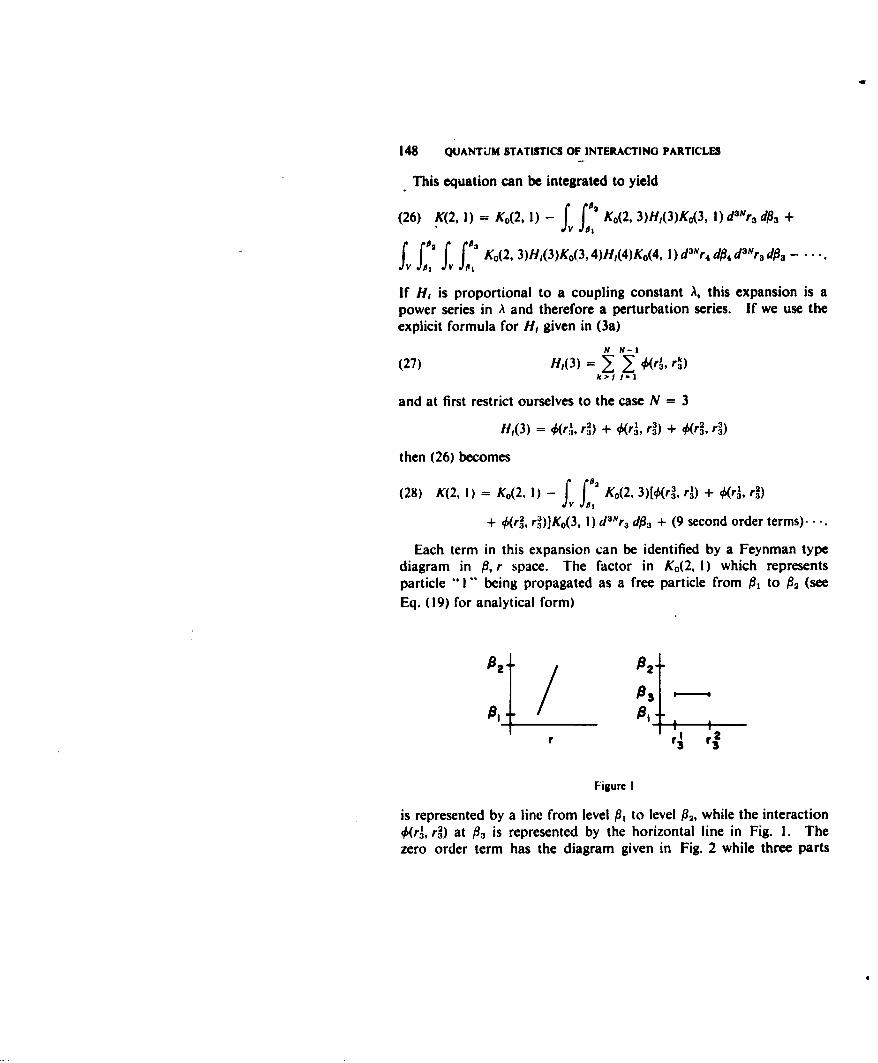
148 QUANTUM STATISTICS OF INTERACTING PARTICLES
This equation can be integrated to yield
(26) K(2, 1) = K0(2, I) - Jf Ko(2, 3)H,(3)K0(3, 1)dr3N r3 dA +V 1
f fi' f, f~if X(2,3)H,(3)Ko(3, 4)ll,(4)Ko(4, I) dN r4dfl4 r 'r3 dfi . .
If H, is proportional to a coupling constant A, this expansion is apower series in A and therefore a perturbation series. If we use theexplicit formula for H, given in (3a)
N N-1
(27) H,(3) = 0 Z,(rl, r')k>1 1-1
and at first restrict ourselves to the case N = 3
H1(3) = 0(r. r ) + 0r' r') + Or. 2 )3 3 3 3 r3 r3•
then (26) becomes
(28) K(2, 1) = Ko(2, I) - f# 2 K0(2, 3)[r, 4r) + r, r2)
+ 34. r)JK0(3, 1) daNr dfl3 + (9 second order terms). -.
Each term in this expansion can be identified by a Feynman typediagram in P, r space. The factor in Ko(2, I) which representsparticle "I - being propagated as a free particle from fl to / 2 (seeEq. (19) for analytical form)
r rI r 2
3 3
Figure I
is represented by a line from level P, to level 2, while the interaction#4r., r2) at 93 is represented by the horizontal line in Fig. I. Thezero order term has the diagram given in Fig. 2 while three parts
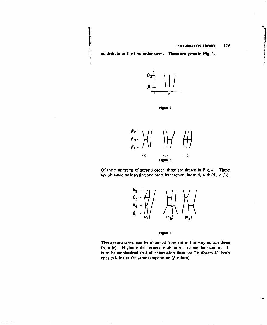
PERTURBATION THEORY 149
contribute to the first order term. These are given in Fig. 3.
Figure 2
02
03-
(a) (b) (C)Figure 3
Of the nine terms of second order, three are drawn in Fig. 4. Theseare obtained by inserting one more interaction line at #4 with (94 < 9 3).
03-
04
(as) (a2) (a3)
Figure 4
Three more terms can be obtained from (b) in this way as can threefrom (c). Higher order terms are obtained in a similar manner. Itis to be emphasized that all interaction lines are "isothermal," bothends existing at the same temperature (P values).
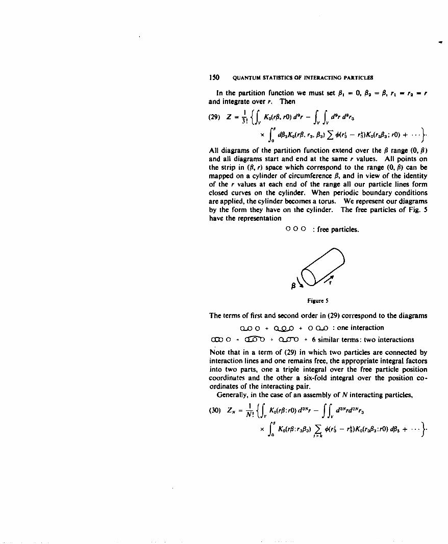
150 QUANTUM STATISTICS OF INTERACTING PARTICLES
In the partition function we must set #1 = 0, 02 = P, r, = r= rand integrate over r. Then
(29) Z = 1 {fv Ko(rP, rO) d 9r - fv fv d'r d'r 33!ff -r)o(Va r0+
SdP:Ko(r#, r3, P.) -0(r )K(r 3 3; rO) + .
All diagrams of the partition function extend over the 9 range (0, /)and all diagrams start and end at the same r values. All points onthe strip in (fl, r) space which correspond to the range (0, P) can bemapped on a cylinder of circumference /, and in view of the identityof the r values at each end of the range all our particle lines formclosed curves on the cylinder. When periodic boundary conditionsare applied, the cylinder becomes a torus. We represent our diagramsby the form they have on the cylinder. The free particles of Fig. 5have the representation
0 0 0 : free particles.
Figure 5
The terms of first and second order in (29) correspond to the diagrams
an o + c + o Q.o : one interactionCOD 0 + CWO .-X-0 + 6 similar terms: two interactions
Note that in a term of (29) in which two particles are connected byinteraction lines and one remains free, the appropriate integral factorsinto two parts, one a triple integral over the free particle positioncoordinates and the other a six-fold integral over the position co-ordinates of the interacting pair.
Generally, in the case of an assembly of N interacting particles,
(30) ZN fKo(rfl:rO) dNr - f fV d3Nrd2 r
x Ko(rfl:r3 93 ) (Ar3 - rl)Ko(r3Pj:rO) dA3 + . "
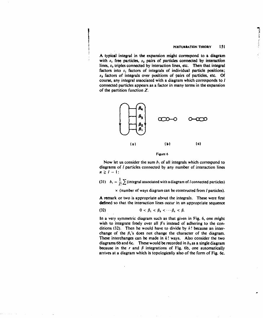
PERTURBATION THEORY 151
A typical integral in the expansion might correspond to a diagramwith s1 free particles, s2 pairs of particles connected by interactionlines, sa triples connected by interaction lines, etc. Then that integralfactors into s, factors of integrals of individual particle positions;s 2 factors of integrals over positions of pairs of particles, etc. Ofcourse, any integral associated with a diagram which corresponds to Iconnected particles appears as a factor in many terms in the expansionof the partition function Z.
02
(al (b) (cl
Figure 6
Now let us consider the sum b, of all integrals which correspond todiagrams of I particles connected by any number of interaction linesn Ž= - I:
(31) b, = I I (integral associated with a diagram of I connected particles)
x (number of ways diagram can be constructed from I particles).
A remark or two is appropriate about the integrals. These were firstdefined so that the interaction lines occur in an appropriate sequence(32) 0 < 91 < 92 < ... flk < /3
In a very symmetric diagram such as that given in Fig. 6, one mightwish to integrate freely over all Pl's instead of adhering to the con-ditions (32). Then he would have to divide by k! because an inter-change of the #ik's does not change the character of the diagram.These interchanges can be made in k! ways. Also consider the twodiagrams 6b and 6c. These would be recorded in b3 as a single diagrambecause in the r and # integrations of Fig. 6b, one automaticallyarrives at a diagram which is topologically also of the form of Fig. 6c.
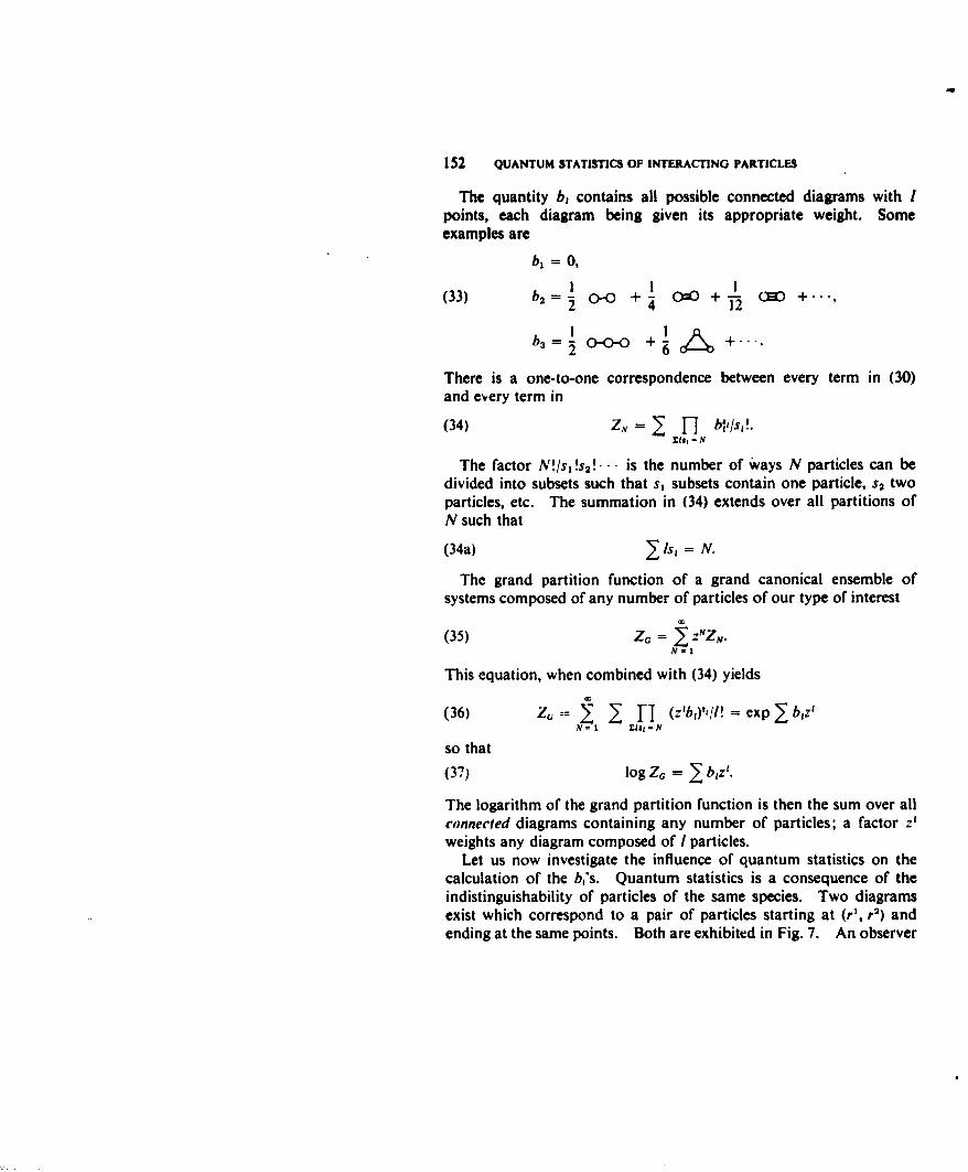
152 QUANTUM STATISTICS OF INTERACTING PARTICLES
The quantity b, contains all possible connected diagrams with Ipoints, each diagram being given its appropriate weight. Someexamples are
bi = 0,
(33) b2 =• 0-0 + 020 + 12 +
21b3 =• 0- + 0 +...
There is a one-to-one correspondence between every term in (30)and every term in
(34) ZN b=,11M/s1!.List - N
The factor N!/s,!s 2 !.. is the number of Ways N particles can bedivided into subsets such that s, subsets contain one particle, s2 twoparticles, etc. The summation in (34) extends over all partitions ofN such that
(34a) Is, = N.
The grand partition function of a grand canonical ensemble ofsystems composed of any number of particles of our type of interest
(35) ZG = 2 :N.N-I
This equation, when combined with (34) yields
(36) ZG = 1 . H (Z'b1 )",/I! = exp : blz'N=1 ZList-N
so that
(37) log ZG = • bz:.
The logarithm of the grand partition function is then the sum over allconnected diagrams containing any number of particles; a factor z'weights any diagram composed of I particles.
Let us now investigate the influence of quantum statistics on thecalculation of the b,'s. Quantum statistics is a consequence of theindistinguishability of particles of the same species. Two diagramsexist which correspond to a pair of particles starting at (r1, r2) andending at the same points. Both are exhibited in Fig. 7. An observer
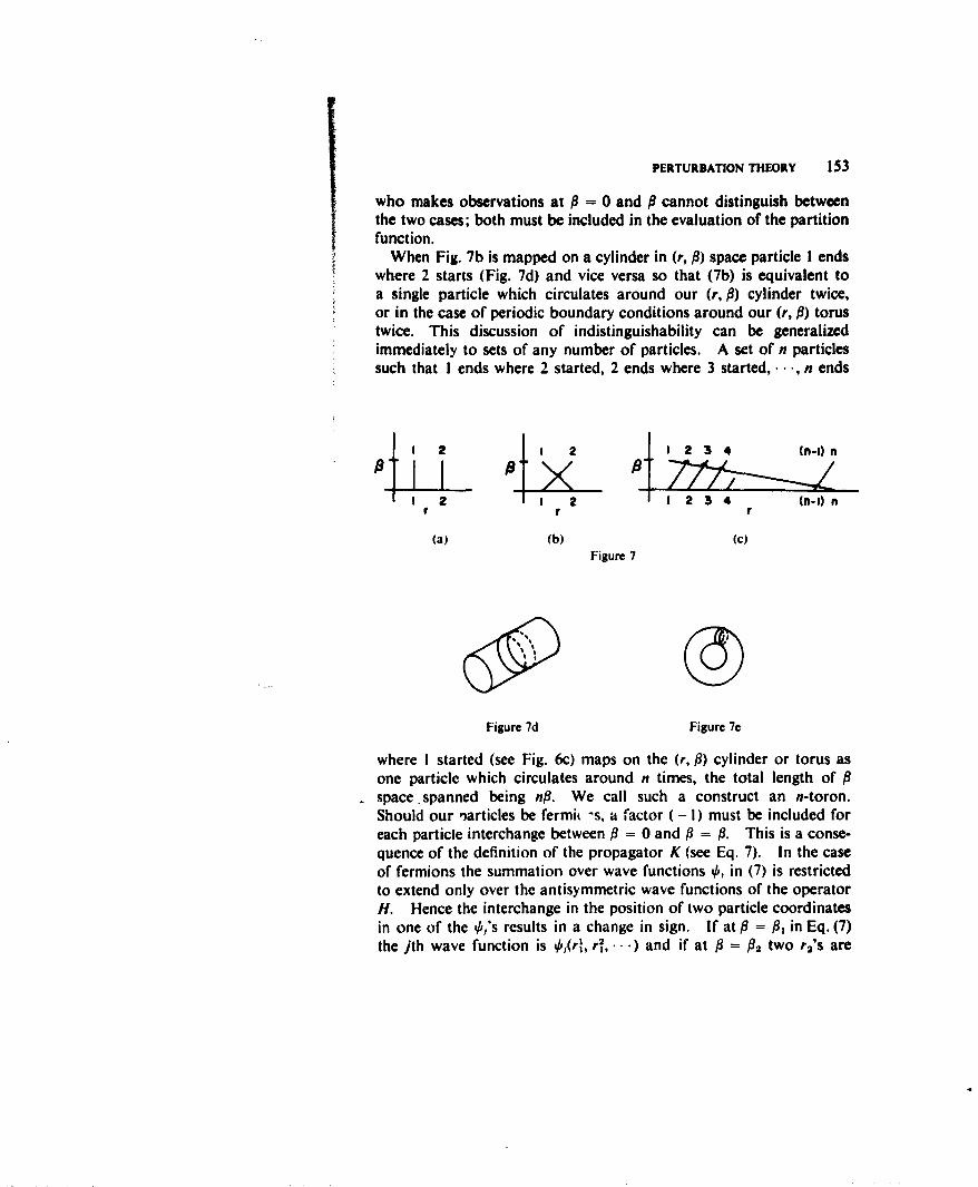
PERTURBATION THEORY 153
who makes observations at/3 = 0 and P cannot distinguish betweenthe two cases; both must be included in the evaluation of the partitionfunction.
When Fig. 7b is mapped on a cylinder in (r, P) space particle I endswhere 2 starts (Fig. 7d) and vice versa so that (7b) is equivalent toa single particle which circulates around our (r, P) cylinder twice,or in the case of periodic boundary conditions around our (r, 9) torustwice. This discussion of indistinguishability can be generalizedimmediately to sets of any number of particles. A set of n particlessuch that I ends where 2 started, 2 ends where 3 started, , n ends
I 2 I 1 2 3 4 (n-) n
1 2 1 2 123401r r r
(a) (b) (C)Figure 7
Figure 7d Figure 7e
where I started (see Fig. 6c) maps on the (r, P) cylinder or torus asone particle which circulates around n times, the total length of Pspace spanned being n/l. We call such a construct an n-toron.Should our narticles be fermit -s, a factor ( - I) must be included foreach particle interchange between P = 0 and P = P. This is a conse-quence of the definition of the propagator K (see Eq. 7). In the caseof fermions the summation over wave functions 0, in (7) is restrictedto extend only over the antisymmetric wave functions of the operatorH. Hence the interchange in the position of two particle coordinatesin one of the 0,'s results in a change in sign. If at/P = /1 in Eq. (7)the jth wave function is 0,j(r, r',.*) and if at # = 92 two r2 's are
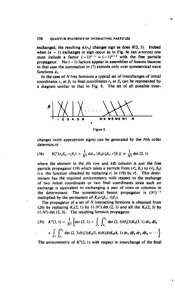
154 QUANTUM STATISTICS OF INTERACTING PARTICLES
exchanged, the resulting 0#(r2) changes sign as does K(2, 1). Indeedwhen (n - I) exchanges in sign occur as in Fig. 6c (an n-toron) onemust include a factor (- I )n - I = ( I )0l +I with the free particlepropagator. No ( - I) factors appear in assemblies of bosons becausein that case the summation in (7) extends only over symmetrical wavefunctions 0,.
In the case of N free fermions a typical set of interchanges of initialcoordinates r, at P, to final coordinates r2 at #2 can be represented bya diagram similar to that in Fig. 8. The set of all possible inter-
1 2 3 4 5 6 N-4 N-3 N-2 N-I Nr
Figure 8
changes (with appropriate signs) can be generated by the Nth orderdeterminant
I I(38) K/,"(r 29 2. ri,) = .detN {Ko(r29 2 ; rfll)} - det (2, 1)
where the element in the jth row and kth column is just the freeparticle propagator (19) which takes a particle from (rk, #Ir) to (r', P2)(i.e. the function obtained by replacing r' in (19) by rk. This deter-minant has the required antisymmetry with respect to the exchangeof two initial coordinates or two final coordinates since such anexchange is equivalent to exchanging a pair of rows or columns inthe determinant. The symmetrical boson propagator is (N!)-'multiplied by the permanent of Ko(r'ji.4,; rk/ 1).
The propagator of a set of N interacting fermions is obtained from(26) by replacing Ko(2, I) by (I/N!) det (2, 1) and all the K0(2, 3) by(I/N!) det (2, 3). The resulting fermion propagator
(39) K'(2, I) = . det (2, I) - f3 det (2, 3)H1(3)K 0(3, l)dr3 df#3
+ f i3 det (2, 3)HI(3)K0(3, 4)H,(4)Ko(4, 1) dr4 d#4 dr3 d#3
The antisymmetry of K'(2, 1) with respect to interchange of the final
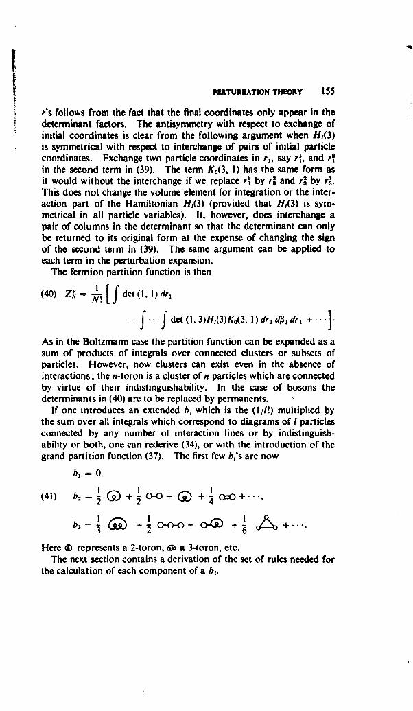
PERTURBATION THEORY 155
r's follows from the fact that the final coordinates only appear in thedeterminant factors. The antisymmetry with respect to exchange ofinitial coordinates is clear from the following argument when H,(3)is symmetrical with respect to interchange of pairs of initial particlecoordinates. Exchange two particle coordinates in r1, say rl, and r2
in the second term in (39). The term Ko(3, I) has the same form asit would without the interchange if we replace r4 by r3 and r3 by r4.
This does not change the volume element for integration or the inter-action part of the Hamiltonian H1(3) (provided that HI(3) is sym-metrical in all particle variables). It, however, does interchange apair of columns in the determinant so that the determinant can onlybe returned to its original form at the expense of changing the signof the second term in (39). The same argument can be applied toeach term in the perturbation expansion.
The fermion partition function is then
(40) ZNF . det(l, l)dri
- f...f det(I,3)HP3)Ko(3, l)dr3 d AdrI +.
As in the Boltzmann case the partition function can be expanded as asum of products of integrals over connected clusters or subsets ofparticles. However, now clusters can exist even in the absence ofinteractions; the n-toron is a cluster of n particles which are connectedby virtue of their indistinguishability. In the case of bosons thedeterminants in (40) are to be replaced by permanents.
If one introduces an extended b, which is the (I//!) multiplied bythe sum over all integrals which correspond to diagrams of I particlesconnected by any number of interaction lines or by indistinguish-ability or both, one can rederive (34), or with the introduction of thegrand partition function (37). The first few b,'s are now
,= 0.I 1 1
(41) b, CD + O-.O+ (ýD + O =0+
++..
Here 4 represents a 2-toron, S a 3-toron, etc.The next section contains a derivation of the set of rules needed for
the calculation of each component of a b,.
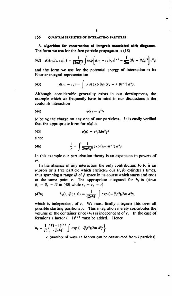
156 QUANTUM STATISTICS OF INTERACTING PARTICLES
3. Algorithm for construction of integrals assocalted with diagrams.The form we use for the free particle propagator is (18)
(42) K0 rA,% rlf 1) (2= I) exp &~2 - rjph1) -- ý9 Ip ~and the form we use for the potential energy of interaction is its
Fourier integral representation
(43) 0(r2 - r1) = f u(q)exp [iq.(r 2 - r)h/-1] d3q.
Although considerable generality exists in our development, theexample which we frequently have in mind in our discussions is thecoulomb interaction
(44) 0r) = e2/r
(e being the charge on any one of our particles). It is easily verifiedthat the appropriate form for u(q) is
(45) u(q) = e2/2hnr2q2
since
(46) =f ' 2 exp (iq. rh - 1) d3q.
In this example our perturbation theory is an expansion in powers of2e .
In the absence of any interaction the only contribution to b, is anI-toron or a free particle which cncirclc:i our (r, f) cylinder I times,thus spanning a range I4 of P space in its course which starts and endsat the same point r. The appropriate integrand for b, is (sinceP2 - P, = 49 in (40) while r2 = ri = r)
(47a) Ko(r, I11; r, 0) = (2 1) exp (-lpp2)/2n d3p,
which is independent of r. We must finally integrate this over allpossible starting positions r. This integration merely contributes thevolume of the container since (47) is independent of r. In the case offermions a factor (- 1) + must be added. Hence
b,= p (1); f exp (-Ifp2 )/2mn d3p}
x (number of ways an l-toron can be constructed from I particles).
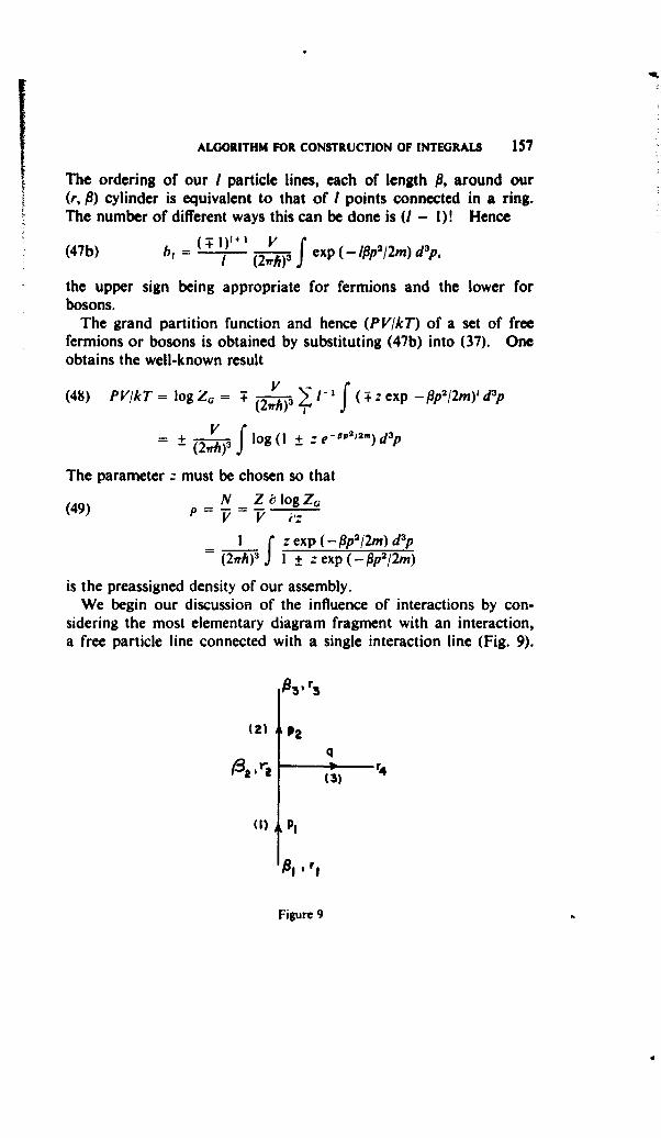
ALGORITHM FOR CONSTRUCTION OF INTEGRALS 157
The ordering of our I particle lines, each of length Pi, around our(r, P) cylinder is equivalent to that of ! points connected in a ring.The number of different ways this can be done is (I - 1)! Hence(47b) b J(Il (3xp (_ lfp 2/2m) d3p,
I (27wh) j
the upper sign being appropriate for fermions and the lower forbosons.
The grand partition function and hence (PVIkT) of a set of freefermions or bosons is obtained by substituting (47b) into (37). Oneobtains the well-known result
(48) PV/kT= logZ. = T (2 3 1-f (s-zexp -fip 2/2m)'d 3pv 2r f _pl. ~
= V ( f log(I +_ :eaP 2- )dap
The parameter Z must be chosen so that
(49) N ZclogZG
I zexp(-Pp2 /2m)dap(2h)3 j 1 I ± z exp (-_p 2 /2m)
is the preassigned density of our assembly.We begin our discussioa of the influence of interactions by con-
sidering the most elementary diagram fragment with an interaction,a free particle line connected with a single interaction line (Fig. 9).
(2) P2
q02 *3 'r4
(I) Pl
Figure 9
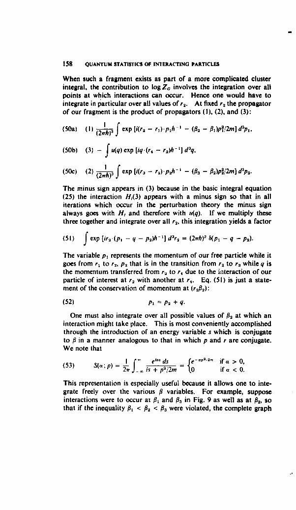
158 QUANTUM STATISTICS OF INTERACTING PARTICLES
When such a fragment exists as part of a more complicated clusterintegral, the contribution to log ZG involves the integration over allpoints at which interactions can occur. Hence one would have tointegrate in particular over all values of r2. At fixed r2 the propagatorof our fragment is the product of propagators (1), (2), and (3):
(50a) (I) f exp [i(r 2 - r,).ph• hI - (/2 - P,)p2 /2m] d3p1,
(50b) (3) - f u(q) exp [iq.(r 4 - r2)h'1]d3 q.
(c) (2) f exp [i(r 3 - r2).ph-' - (93 - P2)p 2/2m] d3p 2 .
The minus sign appears in (3) because in the basic integral equation(25) the interaction H,(3) appears with a minus sign so that in alliterations which occur in the perturbation theory the minus signalways goes with H, and therefore with i(q). If we multiply thesethree together and integrate over all r2 , this integration yields a factor
(51) f exp [irV.(pI - q - p2)h-I] d3r2 = (2wrh) 3 8(pG - q - P2).
The variable p, represents the momentum of our free particle while itgoes from r, to r2 , P2 that is in the transition from r2 to r3 while q isthe momentum transferred from r, to r, due to the interaction of ourparticle of interest at r2 with another at r,. Eq. (51) is just a state-ment of the conservation of momentum at (r2 #2):
(52) p 1 = p 2 + q.
One must also integrate over all possible values of 92 at which aninteraction might take place. This is most conveniently accomplishedthrough the introduction of an energy variable s which is conjugateto # in a manner analogous to that in which p and r are conjugate.We note that
(5) e'a' ds { 2/21" if a >0,
(53)p/2m = if)
This representation is especially useful because it allows one to inte-grate freely over the various P variables. For example, supposeinteractions were to occur at P1 and #3 in Fig. 9 as well as at P2, SO
that if the inequality P, < #2 < Pz were violated, the complete graph
ALGORITHM FOR CONSTRUCTION OF INTEGRALS 159
of which Fig. 9 is a fragment would change its shape. Through useof a representation similar to (53) for the Gaussian in (I) and (2)one would be able to integrate freely on 92 from - oo to + oo becausethe integral would vanish automatically when #2 extended beyondits allowed range (#, Ps),
We are now in a position to derive general rules for the constructionof the integral associated with an arbitrary diagram such as thatgiven in Fig. 10. We do this by first finding a simple expression for
Figure 10
a single toron fragment of such a diagram. Then we find rules forcombining torons. Fig. II represents a typical N toron with ninteraction lines at
(54) 0 < 91 < 92 <... < P < Nfl.
The momentum transfer at these points is
qj, q2," " ",qj.
Our N-toron has been mapped into a circle of circumference NP, thefirst turn when constructed on our (r, P) cylinder is included in therange (0, P), the second turn in the range (fl, 2P), etc. We denote thefull propagator associated with the fragment in Fig. I I by
(55) FN(rrýr2 . . 1#2 ... ).
The translational and periodic symmetry of a toron is such that atranslation of all interaction points by an amount P leads to exactlythe original diagram again. This would weight the same diagramtwice. In order to avoid such a multiple weighting, we restrict theinteraction 9, to the interval (0, P)
(56) 0 < P, < P.
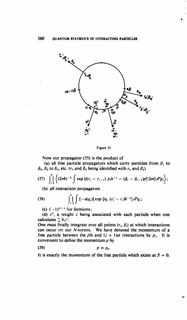
160 QUANTUM STATISTICS OF INTERACTING PARTICLES
PP0
Figure I I
Now our propagator (55) is the product of(a) all free particle propagators which carry particles from Px to
P2, 92 to 93, etc. (ro and fo being identified with r, and f)
(57) L{(2.h) 3f exp [i(r, - r_ 1) -ph - - (#I, - P ~22]d
(b) all interaction propagators
(58) hf [-u(q,)] exp [iq,.(r;-r)h-I] d-q,;
(c) (l+ I for fermions;(d) :, a weight : being associated with each particle when one
calculates > b,:'.One must finally integrate over all points (r,, #,) at which interactionscan occur on our N-torons. We have denoted the momentum of afree particle between the jth and (j + I)st interactions by p,. It isconvenient to define the momentum p by
(59) p = pR.
It is exactly the momentum of the free particle which exists at .= 0.
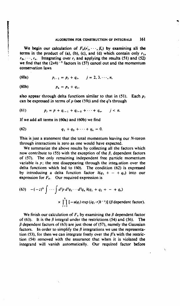
IALGORITHM FOR CONSTRUCTION OF INTEGRALS 161
We begin our calculation of F, , r •,) by examining all theterms in the product of (a), (b), (c), and (d) which contain only rl,r2,.. •., r.. Integrating over r, and applying the results (51) and (52)we find that the (2Qrh) - factors in (57) cancel out and the momentumconservation laws
(60a) pyI = p + q1, j = 2, 3..*-, n,
(60b) Pn = P, + q1,
also appear through delta functions similar to that in (51). Each pican be expressed in terms of p (see (59)) and the q's through
(61) p) =P +q ,+ 1 +q q+ 2 +**+qn, j < n.
If we add all terms in (60a) and (60b) we find
(62) q, +q2 +-" +q. =0.
This is just a statement that the total momentum leaving our N-toronthrough interactions is zero as one would have expected.
We summarize the above results by collecting all the factors whichnow contribute to (55) with the exception of the fP, dependent factorsof (57). The only remaining independent free particle momentumvariable is p, the rest disappearing through the integration over thedelta functions which led to (60). The condition (62) is expressedby introducing a delta finction factor 8(q, + - + q.) into ourexpression for F.,. Our required expression is
(63) -(-:-)'f f dapd:'q.. .d 3q. 8(q, + q2 + - + q.)
x -I - u(q,) exp (iq,. r~h-1)1 (9 dependent factor).
We finish our calculation of F, by examining the P dependent factorof (63). It is the P integral under the restrictions (54) and (56). TheP dependent factors of (63) are just those of (57), namely the Gaussianfactors. In order to simplify the P integrations we use the representa-tion (53), for then we can integrate freely over the Ps with the restric-tion (54) removed with the assurance that when it is violated theintegrand will vanish automatically. Our required factor before
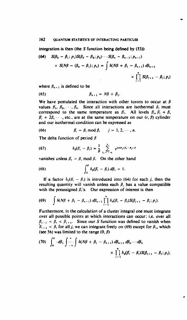
162 QUANTUM STATISTICS OF INTERACTING PARTICLES
integration is then (the S function being defined by (53))
(64) S(A2 - fl,;p,)S(f3 - fl2;p2)...S(f0. - P.-p-P
x S(Nj9 - (ft. - PI);p.) = f S(N + P, - &t. 1) dp.+
X S(Pi + "-f.l; Ps)
where fP,. is defined to be
(65) flP÷i = Nfl + fl#.
We have postulated the interaction with other torons to occur at fPvalues flP, fl2,..., flP. Since all interactions are isothermal Pjy mustcorrespond to the same temperature as fl,. All levels #;, P; + P,fl; + 2fl, •., etc., are at the same temperature on our (r, f9) cylinderand our isothermal condition can be expressed as
(66) fl = fl, mod fl, j= , 2,..., n.
The delta function of period fP
(67) •8(#; - flA) = 2 (,8-)
vanishes unless fl = fP, mod fP. On the other hand
(68) SO(f; - fl,) dfl, = .
If a factor 8•(P - fl,) is introduced into (64) for each j, then theresulting quantity will vanish unless each ft, has a value compatiblewith the preassigned fls. Our expression of interest is then
(69) fS(NP + ft, - fl, 1)dp,,+ I so(#' - P%)SCfl, 1 - p,).f 1=11
Furthermore, in the calculation of a cluster integral one must integrateover all possible points at which interactions can occur; i.e. over all
-, < #I < f, . Since our S function was defined to vanish when4 1 < fP, for all j, we can integrate freely on (69) except for #I, which
(see 56) was limited to the range (0, ft)(70) f" .df, f- f S(NP• + #I, - ft.. 1) dl.÷, IA....dA
X H1 SO(fi - fl,)S(fl, + 1 - fl,; p,).,~i
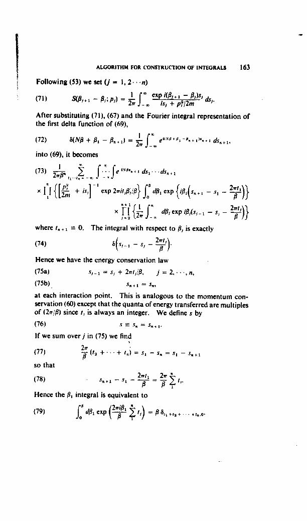
ALGORITHM FOR CONSTRUCTION OF INTEGRALS 163
Following (53) we set (j= ,2..n)
(71 S8,I f exP i(PJ+ 1 - Pds ds,.(71)Pj; ) = , f is1 + p?2/2M
After substituting (71), (67) and the Fourier integral representation ofthe first delta function of (69),
(72) B(NP + P, - += 1) e e(Na + ds" +1,
into (69), it becomes
(73) e .. 1: " . ,ds, ... ds, +
Il 2 fj {[p + is,]-1 exp 21rit,#;/fl } d# exp A ( +s - S1 - P
x F{/LJ dp% exp ip,(s, - s,2-1rtil
where t. + 0. The integral with respect to f, is exactly
(74) 8(s ,-s,- S 2) .
Hence we have the energy conservation law
(75a) s, 1 = s, + 21rt,/P, j = 2,.. n,
(75b) S,,÷ = sR,
at each interaction point. This is analogous to the momentum con-servation (60) except that the quanta of energy transferred are multiplesof (217/g) since t, is always an integer. We define s by
(76) s s. =s.+,.
If we sum over j in (75) we find
(77) 0 2 + + 1.) = si s. = S - sR+1
so that2,fft, 2vr R
(78) s2, • - s1 2 w"P Pr
Hence the #I integral is equivalent to
(79) dfl, exp (f t = p 8i+ea+... *tR..fo, P9811+t2+ 8R,0
164 QUANTUM STATISTICS OF INTERACTING PARTICLES
The s integrations are carried out successively with the aid of (69) and(70) starting with s. 1 and ending with s,. Expression (73) reduces to
(80) 28-1 +t +t... ds e"ON|1 'i OD f- -
X fl.ef yihD[ + is,] 1
where
(81a) sJ =s + 7 (t,+ + + t), j<n,
(81b) S, = S, p pl,
and the other p's are related to p and the q's by (61). Eq. (80) is justthe P dependent factor which must be inserted into (63).
At this stage it should be noted that one can very well collect acomplete class of fragments of diagrams together; namely, all thosewhich are torons similar to Fig. II with n interaction lines. If weinsert (80) into (63) and sum over all N from I to oo, we find a singleexpression(82) F(r;, r'2. .. ;["[.. .')= • F,(ri, . P..[")
f .. f'"d3 q, ... dXq.#-" S(q +'"+q.) St'",,.+
x A,(qt,,.. - qn1.) I1 {-u(q,) exp i[q,.r,/h- + 2rt,f,/fl]}
where(83) A.(q 1 1t...q.t,) = f... d3p ds %(is) H is' +
f 1~=1 2
and•zefil/(I + :eies) Fermi Dirac,
(84) Ois) = ze'8'/(l - :etla) Einstein Bose,: ze'fs Maxwell Boltzmann.
The Fermi Dirac form of w(is) follows immediately from (63) and(82). The Einstein Bose case follows after the minus signs areremoved from the term in front of the integral sign in (63). TheMaxwell Boltzmann result corresponds to the case N = I in (63),since in this classical limit only torons of order one occur.
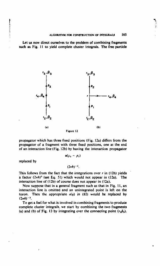
ALGORITHM FOR CONSTRUCTION OF INTEGRALS 165
Let us now direct ourselves to the problem of combining fragmentssuch as Fig. I I to yield complete cluster integrals. The free particle
r4 11 4 r
P 1 P 1
r 2, 02 '2 , 2
(a) (b)Figure 12
propagator which has three fixed positions (Fig. 12a) differs from thepropagator of a fragment with three fixed positions, one at the endof an interaction line (Fig. 12b) by having the interaction propagator
U(P2 - PI)
replaced by
(21h)- 3.
This follows from the fact that the integrations over r in (12b) yieldsa factor (2nh)' (see Eq. 51) which would not appear in (12a). Theinteraction line of (12b) of course does not appear in (12a).
Now suppose that in a general fragment such as that in Fig. II, aninteraction line is omitted and an unintegrated point is left on thetoron. Then the appropriate u(q) in (82) would be replaced by(2vh)- 3.
To get a feel for what is involved in combining fragments to producecomplete cluster integrals, we start by combining the two fragments(a) and (b) of Fig. 13 by integrating over the connecting point (r2, 2).
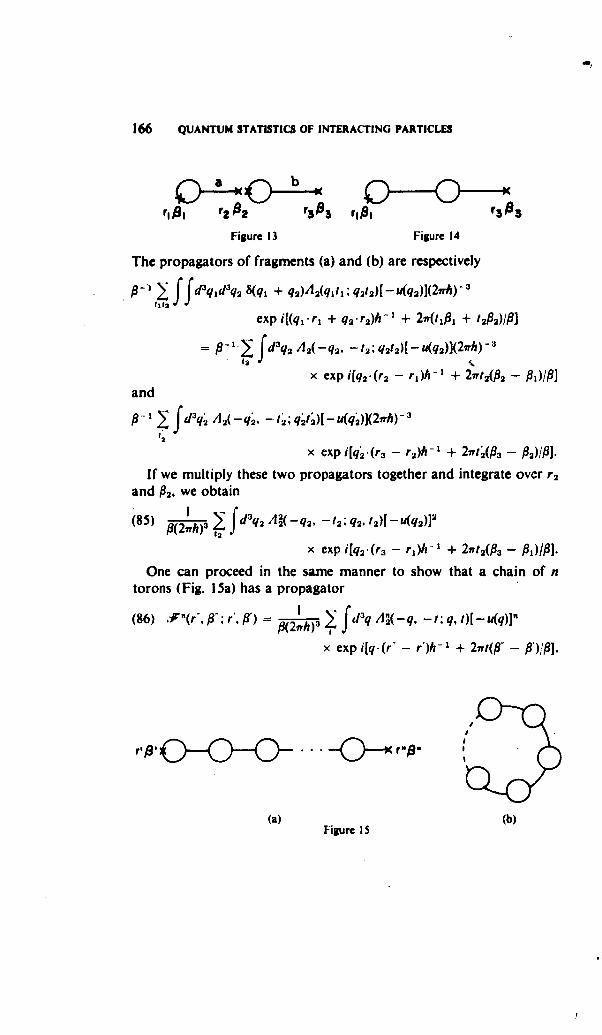
166 QUANTUM STATISTICS OF INTERACTING PARTICLES
rOP r2 22 r3 0 3 rd9P r3 • 3
Figure 13 Figure 14
The propagators of fragments (a) and (b) are respectively
91 fd 3qq1 dq3 8(q, + qO)AA(q, 1 1; q212)[- u(q 2)](2-h) -3
exp i[(q1 *r, + q2 r2)h -1 + 2v(tfl1 + t2fl2)/#]
= 1 fd3q2 A2(-q 2, -1; q 212)[_-u(q2)](2wh)
x exp i[q2 .(r2 - rj)h-1 + 2wt20 2 - #I)/#]
and
9- f d 3q'2 A 2(-q'2 , -1';q'2 t)[-u(q2 )](21rh)-3
f2
x exp i[q'2 (r3 - r 2)h2-1 + 2t12(f3 - ].
If we multiply these two propagators together and integrate over r2
and #2, we obtain
(85) (2h f dq 2 A3(-q 2, -t2; q2, t 2)[-u(q2)]'
x exp i[q2 .(r 3 - rl)h/-1 + 2--t 2(f93 - #I)/#]-
One can proceed in the same manner to show that a chain of ntorons (Fig. 15a) has a propagator
(86) .f'(r, fi; r', ') )3 fd3q A2(-q, -t; q, t)[-u(q)]"
x exp i[q.(r- - r')h - + 2it(fl" -
(a) (b)Figure 15
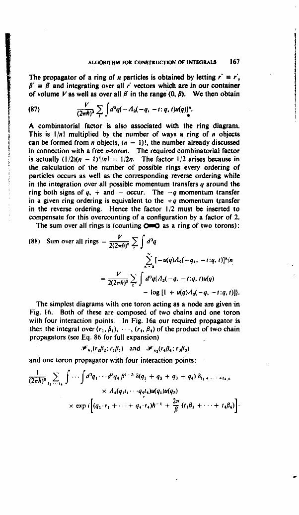
ALGORITHM FOR CONSTRUCTION OF INTEGRALS 167
The propagator of a ring of n particles is obtained by letting r' B r',a P- and integrating over all r' vectors which are in our container
of volume V as well as over all ff in the range (0, P). We then obtain
(87) V- 3 f daq{- A.(-q,-t: q, t)u(q)}3 .(2iv)
A combinatorial factor is also associated with the ring diagram.This is l/n! multiplied by the number of ways a ring of n objectscan be formed from n objects, (n - I)!, the number already discussedin connection with a free n-toron. The required combinatorial factoris actually (1/2)(n - l)!In! = 1!2n. The factor 1/2 arises because inthe calculation of the number of possible rings every ordering ofparticles occurs as well as the corresponding reverse ordering whilein the integration over all possible momentum transfers q around thering both signs of q, + and - occur. The -q momentum transferin a given ring ordering is equivalent to the +q momentum transferin the reverse ordering. Hence the factor 1/2 must be inserted tocompensate for this overcounting of a configuration by a factor of 2.
The sum over all rings is (counting 0 as a ring of two torons):
(88) Sum over all rings = 2 )3 : d3q
7 [- u(q)A2(-q 1, - I:q, t)]R/nR=2
2(2Vh)3 • f d3q{A 2(-q, -t:q, t)u(q)- log [I + u(q)A 2(-q, -t:q, 1)]}.
The simplest diagrams with one toron acting as a node are given -inFig. 16. Both of these are composed of two chains and one toronwith four interaction points. In Fig. 16a our required propagator isthen the integral over (r,, #1), • - -, (r4, f#1 ) of the product of two chainpropagators (see Eq. 86 for full expansion)
.F",I(r 2 •2 . rrfl1 ) and .F'=2 (r4f 4 ; r3fl 3)
and one toron propagator with four interaction points:
Sf...fdq,. .. d'q4 flP-_ F(q, + q2 + qa + q 4 ) 8,, + +4.o
x A4(qit 1"" "q4 ti)u(q1)u(q3)
x expi1 (q*.r .+ q4 r + 0fl + '+ 14fl4)].
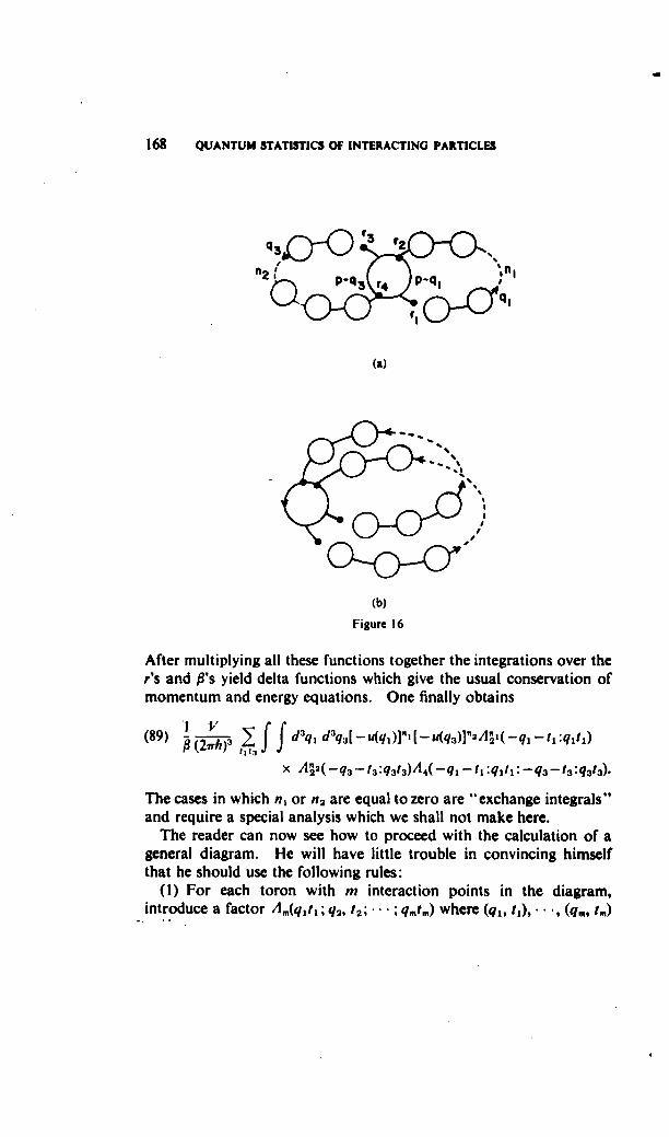
168 QUANTUM STATISTICS OF INTERACTING PARTICLES
b P'q3 r4 p.•
(a)
0-0--
(b)
Figure 16
After multiplying all these functions together the integrations over ther's and P's yield delta functions which give the usual conservation ofmomentum and energy equations. One finally obtains
(89) 1 (2V) 3 , f f d3q1 d3q 3l[-u(q)]"'[-u(q3)]j"A"'(-q 1 -t 1 :qltl)
x 22( -q 3 - t3 :q3t3)A 4( -ql -tl :qltl: -q 3 - t3:q3t3).
The cases in which n1 or n2 are equal to zero are "exchange integrals"and require a special analysis which we shall not make here.
The reader can now see how to proceed with the calculation of ageneral diagram. He will have little trouble in convincing himselfthat he should use the following rules:
(I) For each toron with m interaction points in the diagram,introduce a factor Am(qiti ; q 2, t2;.., ; qmt.) where (qj, tj),.., (q., t.)
ALGORITHM FOR CONSTRUCTION OF INTEGRALS 169
are the amounts of momentum and energy lost at each interactionpoint.
(2) For each interaction line of momentum, q, introduce the factor- u(q).
(3) Introduce a factor P- where I is the total number of torons.and I the number of interaction lines in the diagram.
(4) Integrate the product of the above factors over all momentumtransfers and sum over all energy transfers (energy being transferredin quanta of magnitude 2ait/!, t being an integer). The conservationlaws are to be applied at each interaction point on a toron.
(5) Introduce a factor V/(21rl) 3.(6) Introduce the combinatorial factor (I0I!2") (number of ways
diagram can be drawn) where I = number of torons and n is thenumber of independent paths along which momentum can be trans-ferred.
The factor V(21h)-3 arises from the fact that the last delta functionin dealing with momentum conservation in particle propagators is tobe interpreted (see Eq. 23) as V8p,, 2(2rh)-3. The physical signifi-cance of the V is that all interactions depend only on relative coor-dinates. Hence in the configurational form of the partition function,the integration over the position of the last particle merely contributesthe volume of the container.
The origin of the factor i - I is as follows. In the (r, fP) representa-tion of the grand partition function, the ith toron propagator of acomplex diagram composed of I torons has the P containing factor1-1 1 (l/gIP') = P-" 2, since the total number of interaction points,: n,, is twice the number of interaction lines 1. The interaction linesrepresent isothermal interactions, both ends of the line being associatedwith the same temperature. Hence in the final P integrations, afactor 9 appears for each line, yielding a total factor #I. Whenmultiplied by the above #1 - 21, we obtain the P'- mentioned in rule 3.
In order to perform detailed calculations, one must have explicitexpressions for the A's rather than their integral representations.Although the 4-fold integrations (83) are relatively straight-forward(at low temperatures they proceed in a manner similar to the usualSummerfeld method for integrals which appear in the perfect FD orEB gas) the required expressions are quite long except for the casen = 2. A- detailed investigation of these integrals is contained in aforthcoming review of the statistical mechanics of an electron gas.Here we merely record a few asymptotic results for A2 ( -q, -t; q, t)(see reference 15).
170 QUANTUM STATISTICS OF INTERACTING PARTICLES
In the Maxwell Boltzmann statistics
(90a) A2(-q, 0; q, 0) = (n + 2,n)!
~ (P [,!)aI + O(q2)] as q -* 0
(90b)- -4- + O(q- 4) as q -o.
Ift 9 Oand
(91) A2(-q, -t;q,t) q2 +m( 2.ml 3! + O(/lq2[l + ()lq2)2j)}
(92) r = 27rmt/p,
when either q2 >> 2m/P or (Qr/q)2 >> 2m/!P.In the FD case as P--* c for fixed Q and V
1 ) mpo 4Q + [I + (V + iQ)2] log [(V + iQ) + iJA2-Q q, t(V + iQ) - i]
(93) + [I + (V - iQ)2] log [(V - iQ) - i]i
iQ2Iog - Q) + ill
where
(94) z = exp - p•fi/2m; V = tq and Q q/2po.fqPO; n lp
It is easily shown from (93) that
f41mpo(l - Vtan'- V- 1) as Q- 0,(95) Aj (-q, -t~q, i) - 4-mpo (2 .V2aQ- 2 0 as Q - oo.
4. Application to a assembly of charged particles. We now applythe general formalism described above to the statistical mechanics ofa gas of negative ions imbedded in a continuum of positive chargewhose charge density is so fixed that the complete assembly is electri-cally neutral. Since our formalism is a systematic perturbationtheory in which log Z; is presented as an expansion in powers of theinter-particle coupling constant (e2 in our case) it is best in the weak
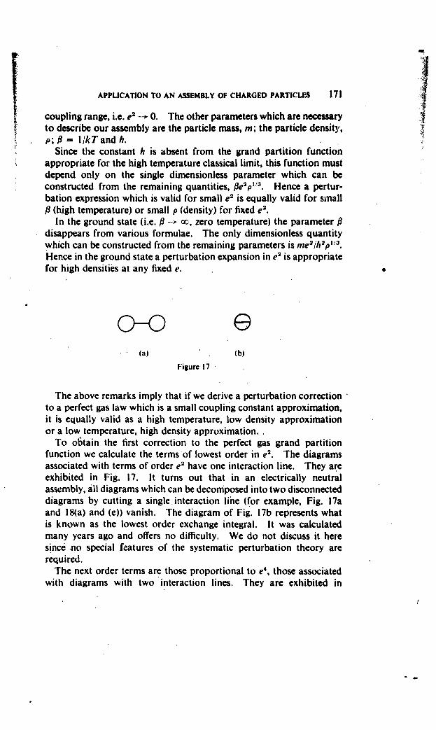
I APPLICATION TO AN ASSEMBLY OF CHARGED PARTICLES 171
coupling range, i.e. e2 -- 0. The other parameters which are necessaryto describe our assembly are the particle mass, m; the particle density,p; P I IkT and h.
Since the constant h is absent from the grand partition functionappropriate for the high temperature classical limit, this function mustdepend only on the single dimensionless parameter which can beconstructed from the remaining quantities, fle2p1 3. Hence a pertur-bation expression which is valid for small e2 is equally valid for smallP (high temperature) or small p (density) for fixed el.
In the ground state (i.e. f - oo, zero temperature) the parameter/fdisappears from various formulae. The only dimensionless quantitywhich can be constructed from the remaining parameters is me 2 /hp 3 .
Hence in the ground state a perturbation expansion in e 2 is appropriatefor high densities at any fixed e.
0-a0
(a) (b)
Figure 17
The above remarks imply that if we derive a perturbation correctionto a perfect gas law which is a small coupling constant approximation,it is equally valid as a high tcmperature, low density approximationor a low temperature, high density approximation..
To o6tain the first correction to the perfect gas grand partitionfunction we calculate the terms of lowest order in e2. The diagramsassociated with terms of order e 2 have one interaction line. They areexhibited in Fig. 17. It turns out that in an electrically neutralassembly, all diagrams which can be decomposed into two disconnecteddiagrams by cutting a single interaction line (for example, Fig. 17aand 18(a) and (e)) vanish. The diagram of Fig. 17b represents whatis known as the lowest order exchange integral. It was calculatedmany years ago and offers no difficulty. We do not discuss it heresince Jno special features of the systematic perturbation theory arerequired.
The next order terms are those proportional to e4, those associatedwith diagrams with two interaction lines. They are exhibited in
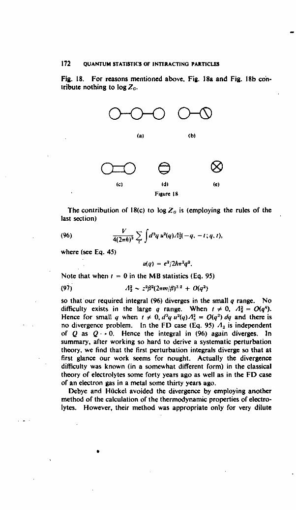
172 QUANTUM STATISTICS OF INTERACTING PARTICLES
Fig. 18. For reasons mentioned above, Fig. 18a and Fig. I8b con-tribute nothing to log ZG.
0-0-0 Q-o(a) (b)
0 © 0(c) (d) (C)
Figurc 18
The contribution of 18(c) to log ZG is (employing the rules of the
last section)
(96) 4(2h) f fdaq u2(q)AR(-q, -t; q, 1),
where (see Eq. 45)
u(q) = e2/2hV2 2q2 .
Note that when t = 0 in the MB statistics (Eq. 95)(97) A' - : 2#2(2-m/#)3,2 + O(q2)
so thatour required integral (96) diverges in the small q range. Nodifficulty exists in the large q range. When t # 0, A 2 = O(q4).Hence for small q when t o 0, d 3q u2(q),1 = 0(q2 ) dq and there is
no divergence problem. In the FD case (Eq. 95) A 2 is independentof Q as Q - 0. Hence the integral in (96) again diverges. Insummary, after working so hard to derive a systematic perturbationtheory, we find that the first perturbation integrals diverge so that atfirst glance our work seems for nought. Actually the divergencedifficulty was known (in a somewhat different form) in the classicaltheory of electrolytes some forty years ago as well as in the FD caseof an electron gas in a metal some thirty years ago.
Debye and Hulckel avoided the divergence by employing anothermethod of the calculation of the thermodynamic properties of electro-lytes. However, their method was appropriate only for very dilute
APPLICATION TO AN ASSEMBLY OF CHARGED PARTICLES 173
solutions and could not be extended to higher concentrations. J. E.Mayer made the correct step to resolve the divergence difficulty in theMB case and Gell-Mann and Brueckner independently used the sameidea in the FD case.
Suppose that instead of fretting over our troubles in the calculationof (96), we go on to the next order nonexchange contribution tolog Za, the ring of three interacting particles
(2rnh)3 > df3dq u3(q)A3(-q, -t: q, t).
This term .is even more divergent than (96). However, the sum overall rings (Eq. 88)
(98) V 3q dqA 2(-q, -t:q, i)u(q)
- log [I + u(q)A 2(-q, -t:q, t)]}
is convergent. For example, if in the MB case we examine the t = 0term and approximate A2 by #(22rmi, jp) 3
2, we have
(99) 2(2wt)V f' 4-q2 dq{2- - log (I +)
where
(100) : = 2m/' 2
2h77'
The above convergent integral has the value
27r2 V, 3 12 2V 2V /:e 2 n)312 2m )3 A.(101) 3(2-hP): = 3(2;h)P -h) \(2#T
Since the perfect gas contribution (I-toron contribution) to thelog Zu is (see Eq. 47) :VIh'/(2/r[!m)3'2, the total contribution of thenoninteracting particle graphs plus ring graphs to log ZG, or toPV/kT is (see Eqs. 48 and 36)
PV= :V 277 2V -~e 2 m) 3'2 (2m) 3 ,4+ T__I-(102) j- = log Z ' = h'(21rp/im), 2 3(27'h).3 ( h T9
while and the density p are related through (Eq. 49)
z i, log Z' # Ir2 (:e2mn\
3'2 2m 3 14(103) P V -P 'z = h3(2lim)3'2 + (2--7• k ]/"
174 QUANTUM STATISTICS OF INTERACTING PARTICLES
Here one is interested in z as el -* 0. In the limit
(104) = pA3(2w/r/)112.
The correction 8z to this value when e is small but finite is obtainedby substituting (104) into the second term on the right hand side of(103) and solving for the z in the first term on the right hand side(104). One obtains
(105) : = (2wr) 312h3(l/M) 312p{l - e 3# 3!2pU 2ff 12 + 0(p)).
Substituting this into (102) we find the Debye-Huckel equation ofstate
(106) PikT = p l I e P2e3,,312p12}
The high pressure ground state energy of an electron gas is obtained
by substituting (93) into (98). As P -x o (T - 0) the parameter
V = 2vtmr/fqpo
becomes a continuous variable even though t is discrete.. The sum-mation with respect to t can be converted to an integral with respectto V. Then (98) becomes (after letting q = q'po and ignoring theprime on q' and allowing for two spin states by replacing u(q)A 2 by2u(q)A 2)
____ f1(,V e2A2(q, V)1i
(107) VP•f q3 dq :: dV{ e'/I2 gq, V) log [1 + e--p2pq- V .
The log Zý is then, to the ring integral approximation,
(108) log1 Z = log ZG°1 + (107)
where Z,,0 is the grand partition function of a perfect Fermi gas.The internal energy is found by differentiating (108) with respect to
Sat constant : = exp #p20/2m; the density by differentiating (108)with respect to z at constant ft. For this purpose we substitutePo = (2mf#-I log Z)1/2 into (108) before carrying out our differentia-tions. The details of the differentiation are tedious but straight-forward. They have been given in some detail in the original paperof Montroll and Ward. As in the classical case we assume thatz = zo + 8z where z0 is now chosen to be exp (flp2/2m) (p, being theFermi momentum h(3,r 2p)" 3. Then the correction 8: is found to
I APPLICATION TO AN ASSEMBLY OF CHARGED PARTICLES 175
keep the density at p. Now one can express the ground state energy(as l-+o) as
E = Eo(z) + 8E(z)
= EO(zo) + 7 8z + 8E(zo)} +.
The first order correction to Ehe free particle contribution to theground state energy has two parts, one being the direct correlationenergy evaluated at z = zo and the second being the change in thefree particle energy due to the fact that : must be changed to yield theproper density. One finally obtains the correlation energy,[E - Eo(:o)], to be
(109) .corr - 3h2 q 3 dq
r dVfe2A 2o._ log [+ eA 2q_ }
where (4/3)frprgo = I and ,, = (4/970)1'3. This is exactly the Gell-Mann-Brueckner formula for the correlation energy per particle ofan electron gas. A detailed discussion of the integral is given in theBrueckner lecture notes of the 1958 lIcole d'L6t de Physique Theorique.Numerically Brueckner finds (in Rydbergs)
E,,orr = -0.096 + 0.0622 In r,
with r, = ro/ra, ra being the Bohr radius.The physical idea behind the removal of the small q divergence is
that each direct interaction between two particles is to be replacedby the sum of -- + 0 + -- 0----- + ... , the directinteraction plus an interaction through an intermediate particle plusone through two intermediates, etc. We examine the consequence ofthis idea in the classical limit. We consider only the terms t = 0,since in our required limit only these terms led to divergences. Thenwe should replace u(q) by
(110) u(q) - A2(-q, 0; q, O)u2 (q) + A'u 3(q). = u(q)/[l + A2u(q)].
From this we can calculate an effective potential to replace the coulombpotential e2 /r. This potential would be just the Fourier transformof (110)
(I I a)f d 3 q ex__p (iq. rh -1 ) e2(Ilia) q 2 [1 + -q -2 -q 2 r
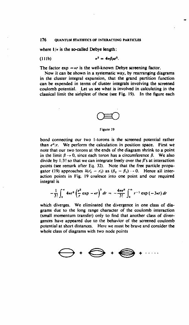
176 QUANTUM STATISTICS OF INTERACTING PARTICLES
where I/K is the so-called Debye length:
(I I lb) of2 = 4-ppe2.
The factor exp - ir is the well-known Debye screening factor.Now it can be shown in a systematic way, by rearranging diagrams
in the cluster integral expansion, that the grand partition functioncan be expended in terms of cluster integrals involving the screenedcoulomb potential. Let us see what is involved in calculating in theclassical limit the sin'plest of these (see Fig. 19). In the figure each
Figure 19
bond connecting our two 1-torons is the screened potential ratherthan e2 /r. We perform the calculation in position space. First wenote that our two torons at the ends of the diagram shrink to a pointin the limit --+ 0, since each toron has a circumference P. We alsodivide by 1/3! so that we can integrate freely over the P's at interactionpoints (see remark after Eq. 32). Note that the free particle propa-gator (19) approaches 8 (r' - rj) as (0 2 - 0)-0. Hence all inter-action points in Fig. 19 coalesce into one point and our requiredintegral is
410 r2 exp - Kr 3 dr = 4 r- I exp (- 3Kr) dr
which diverges. We eliminated the divergence in one class of dia-grams due to the long range character of the coulomb interaction(small momentum transfer) only to find that another class of diver-gences have appeared due to the behavior of the screened coulombpotential at short distances. Here we must be brave and consider thewhole class of diagrams with two node points
+ + +.....
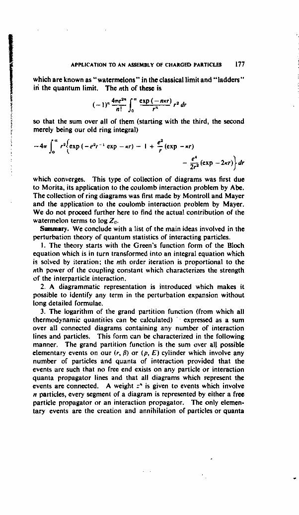
APPLICATION TO AN ASSEMBLY OF CHARGED PARTICLES 177
which are known as "watermelons" in the classical limit and "ladders"in the quantum limit. The nth of these is
-)nn. fo exp (- nnr) r2 dr
so that the sum over all of them (starting with the third, the secondmerely being our old ring integral)
147r r2{exp(-e2r- Iexp -Kr) I + -(exp -Kr)0 r e4
21r2 (exp - 2Kr)} dr
which converges. This type of collection of diagrams was first dueto Morita, its application to the coulomb interaction problem by Abe.The collection of ring diagrams was first made by Montroll and Mayerand the application to the coulomb interaction problem by Mayer.We do not proceed further here to find the actual contribution of thewatermelon terms to log ZG.
Summary. We conclude with a list of the main ideas involved in theperturbation theory of quantum statistics of interacting particles.
I. The theory starts with the Green's function form of the Blochequation which is in turn transformed into an integral equation whichis solved by iteration, the nth order iteration is proportional to thenth power of the coupling constant which characterizes the strengthof the interparticle interaction.
2. A diagrammatic representation is introduced which makes itpossible to identify any term in the perturbation expansion withoutlong detailed formulae.
3. The logarithm of the grand partition function (from which allthermodynamic quantities can be calculated) ` expressed as a sumover all connected diagrams containing any number of interactionlines and particles. This form can be characterized in the followingmanner. The grand partition function is the sum over alI possibleelementary events on our (r, P) or (p, E) cylinder which involve anynumber of particles and quanta of interaction provided that theevents are such that no free end exists on any particle or interactionquanta propagator lines and that all diagrams which represent theevents are connected. A weight z" is given to events which involven particles, every segment of a diagram is represented by either a freeparticle propagator or an interaction propagator. The only elemen-tary events are the creation and annihilation of particles or quanta
I
178 QUANTUM STATISTICS OF INTIMACTING PATICL.
of interaction with energy and momentum being conserved duringthe occurrence of each event. Actually one could start with theseremarks as the basic postulates of statistical mechanics and derive allother results from them.
4. Finally, divergences occur in the evaluation of various clusterintegrals which are associated with our diagrams. These are removedby summing over various classes of diagrams and performing energymomentum transfer integrations after the summation is performed.This is the weak point of the theory as here presented. One has torely on physical plausibility rather than mathematical rigor to haveconfidence in the results. It is not even clear that all divergences canbe dealt with in this way; it just turns out that in the weak couplinglimit, the first few terms in the systematic expansion of thermo-dynamic functions seem to work out well. One optimistically con-tinues, hoping that all is right with the world.
BIBLIOGRAPHY
1. R. Abe, J. Phys. Soc. Japan 14 (1959), 10.2. C. Bloch and C. de Dominicis, Nuclear Phys. 7 (1958), 459; 10
(1959), 181, 509.3. K. A. Brueckner, The many-body problem, 164, Les Houches
(1958).4. R. P. Feynman, Phys. Rev. 76 (1949), 749, 769.5. E. S. Fradkin, Nuclear Phys. 12 (1959), 465.6. M. Gell-Mann and K. A. Brueckner, Phys. Rev. 106(1957), 364.7. J. Goldstone, Proc. Roy. Soc. London Ser. A. 239 (1957), 267.8. The Huang, Lee, and Yang hard sphere gas calculations have
been reviewed by K. Huang, Les Houches (1958).9. J. Hubbard, Proc. Roy. Soc. London Ser. A. 240 (1957), 539.
10. T. D. Lee and C. N. Yang, Phys. Rev. 113 (1959), 1 fk5.11. J. E. Mayer, J. Chem. Phys 18 (1950), 1426.12. P. Martin and J. Schwinger, Phys. Rev. 115 (1959), 1342.13. E. W. Montroll and J. E. Mayer, J. Chem. Phys. 9 (1941), 626.14. E. W. Montroll and J. C. Ward, Phys. of Fluids 1 (1958), 55.15. E. W. Montroll, La thiorie des gaz neutres et ioniz's, 17, Les
Houches (1954).16. T. Morita, Progr. Theoret. Phys. 20 (1958), 920.17. A. Siegert, Physica Supplement 26 (1960), 30.
Index
Abe, 177 corresponding states, law of, 34additivity property, I critical point, 33, 54articulation point, 38 critical temperature, 33
Curtiss, C. F., 57, 140Balescu, R., 139 cycle, 38B-B-G-K-Y hierarchy, 120Berlin, T. H., 59, 140 deBoer, J., 56Binary coilisions, 118, 129 Debye, P., 172Bird, R. B., 57 Debye-Huckel equation of state, 174Birkhoff, 25 Debye length, 176Bloch, C., 144 Debye screening factor, 176Bloch equation, 146 density in phase space, 3Bogoliubov, N. N., 120, 122 disconnected (see graph)Boltzmann, L., 1, 5, 27, 31, 81, 86 dispersion of sound, 89, 96, 99, 109Born, M., 140 distribution function, first, 14, 77, 122Bose gas, 58 --- , s-particles, 14, 121boundary conditions, 109 , temporal development, 122, 123Brueckner, K., 144. 173 distribution, microcanonical surface, 12Burnett. D., 107 u---, p-space, 6
probability density in /-space, 5,Carleman, T., 81, 87 10Case, K. M., 94Caylcy tree, 39, 53 Ehrenfest, P., 25, 28, 29, 31Chang, C. S. Wang, 85, 88 Ehrenfest, T., 25, 28, 29Chapman, S., 112 eigenvalues of linearized collision opera-Chapman-Enskog development, 81,103 tor, 82characteristic function, 13 Einstein, 58chemical potential, 45 energy density, internal, 103, 136Choh. S. T., 135, 139 energy shell, 8cluster, 38 energy surface, 5, 29cluster integral, 38 ensemble, 3cluster-property, 131 ..... , canonical, 16coarse graining, II. 15, 28 , microcanonical, I ICohen. E. G. D., 139, 140 ensemble average, 12collision crom section, 79 ensemble fluid, 3collision operator, 82 Enskog. D.. 88, 112, 139collision parameter, 78 entropy. 22collisions, molecular, 77 equilibrium, approach to, 5, 79condensation phenomenon, 32 -- , thermal, 5conden.,ation, theory of, 72, 75 equilibrium distribution in ju-space, 80conductivity, thermal, 10, 107, 116, 119 equivalence of canonical and grandcontinuity equation, 4, 103, 136 canonical ensemble, 72contraction of description, 15, 110, 123 ergodic theorems, 9, 12convergence question, 58 Eucken constant, 107convergence, radius of, 68 Euler hydrodynamic equations, 104correlation energy of electron gas, 175 Eulerian description, 4
179
180 INDEX
Fermi, E., 29 Hlickel, 172Feynman, R. P., 144 Husimi tree, 39Fierz, M., 30 hydrodynamical equations, 104, 105, 108first law of thermodynamics, 16, 19fluctuations, 9 integral invariant, 26forces, external, 2, 19 interaction potential, 2, 26, 35
-- , intermolecular, 2, Ii, 26, 33, 34, irreversibility, 1, 5, 12751, 78, 83, 85 Irving, J. M., 141
Ford, G. W., 56, 59, 76Fourier law of heat conduction, 105, 138 Jacobian, 4Fowler, R. H., 30 Jeans, 30Fradkin, E. S.. 144Fuchs, W. H. J., 59 Kac, M., 26, 29, 72, 99, 139
Kahn, B., 56, 58F-point, 3 Khinchin, A. J., 25, 29, 31
F-space, 3 Kihara, T., 57
Gaussian model, 51 Kirchhoff, G., 59GclI-Mann, M., 144, 173 Kirkwood, J. G., 120, 139, 141
Gibbs, J. W., I, 3, 9, II, 13 Krnig, D., 56Goldstein, H., 26 Krutkow, G., 31Goldstone, J., 144 Lagrangian description, 4Grad, H., 31, II Igraph, complete, 4 Landau, L. D., 25, 54grap disconnected, 38 Lattice Gas, 75disconneted, 38 Lee, T. D., 56, 66, 72, 75, 144Lennard-Jones (12,6) potential, 26, 34labelled, 37, 4 Lifshitz, E. M., 25
simple, 38 limit property, 62graph complexity, 52 Liouville theorem, 3, 26graph group, 40 Lunbeck, R. J., 56graph garoup, 40graph matrix, 52 macroscopic causality, 15, 117Green. H. S., 140 macroscopic description, 6, 15Green, M. S., 120, 1399 141 macroscopic equations, general, 135Grnecyli)4.1, mL., 0, 99 macroscopic equilibrium, 9Guernsey, R. L., 139 macroscopic observer, 14Guggenheim, E. A., 30 macroscopic variables, 9, 14
main leaves, 47Halmos, P. R., 29 Martin, P., 144Hamiltonian, 2 mass density, 103, 135Hamiltonian operator, 120, 143 Matsubara, 144Hart, R. W., 59 Mayer, J. E., 36, 56, 58, 141, 173, 177heat current density, 103, 136 Mayer, M. G., 56heat, quantity of, 20 Mayer equations, 45Heaviside step function, 145 Mayer theorem, first, 40Hedlund, G. A., 29 -- , second, 47Helmholtz free energy, 24 Maxwell, J. C., 88Hilbert, 117 Maxwell distribution, 8, 28, 80, 132Hilbert paradox, 110 Maxwell model, 85, 88, 99Hirschfelder, J. 0., 57, 108 Maxwell rule, 33, 75Hollinger, H. B.. 140 Melamit, A., 29Hopf, E., 29 metrically transitive property, 12, 13, 29H-theorem, 79, 86, 135 microcanonical ensemble, I IHuang, K., 144 microcanonical surface distribution, 12
INDEX 181
Montroll, E. W., 59, 141, 174, 177 star tree, pure, 39, 47Morita, T., 177 -, rooted, 47MOnster, A., 25 stationary distribution, 5g,.space distribution, 6 stationary stochastic processes, 30
Stern, 0., 31"N!" controversy, 31 Stosszahl-Ansatz, 79Navier-Stokes equations of hydro- streaming in p-space, 77
dynamics, 105 streaming operator, 125Newton law of friction, 105, 138 supersaturation, 61, 62number of labelled (p,k) graphs, 57 symmetry number, 40number of labelled stars, 57
temperature, 16Onnes, Kamerlingh, 34, 36 time average, 12
Tolman, R. C., 25, 27Partition function, canonical, 24, 143 triple point, 54
grand canonical, 43, 66 Trkal, V., 31path. 38"physically infinitesimal", 7 Uhienbeck, G. E., 56, 58, 88Poincar6. H., 26, 29 uniformity parameter, 110Poincark recurrence theorem, 5, 26 Ursell, H. D., 36, 56pressure tensor, 103, 136Prigogine, 1., 120, 139 Van der Waals, 2, 25, 33, 55probability assumption, 10 Van der Waals equation, 73product theorem, 41 Van Hove theorem. 62propagator, 145 Van Kampen. N. G., 88
,fre particle, 146 variables, extensive, 23
quasi-ergodic systems, 29 variables, intensive, 23
quasi-Maxwell model, 85, 106 - , normal, 13
quasi periodic property, 5,9, 1 velocity, average flow, 103, 135- . thermal, 103
rate or strain tensor, 103 virial coefficients, 36, 45, 50
recurrence time, average, 29 virial expansion, 36, 50, 123Riddrell, R.iJ.,e7,avera729 virial expansions of transport coefficients,Riddell, R. J., 57, 58, 72 119Rosenthal, A., 29 viscosity coefficient, 105, 107, 117, 119
Schr6dinger, E., 31 , second, 119
Schr6dinger equation. 143 von Neumann, J., 30
Schwinger, J.. 144second law of thermodynamics, 16, 21 Waldmann, L., 85, 88, 112Sengers, J. V.. 140 Ward, J. C., 144, 174Siegert, A. J. F., 144 Whittaker, E. T., 26Sonine polynomia, 84 work, external, 20spectrum of linearized collision operator,
82 Yang, C. N., 56, 66, 72, 75, 144star, 39 Yvon, J., 140star tree. 39
mixed, 39, 48 zeroth law of thermodynamics, 5, 16