i

Understanding and Development of Inter-cell Interference Mitigation mechanism in LTE-A Heterogeneous Network

Förståelse och utveckling av Inter-interferens Mitigation mekanism i LTE-A

heterogent nätverk

Bilal Shah

Suman Ghimire

Faculty of Health, Science and Technology

Master’s Program in Electrical Engineering

Degree Project of 30 credit points

Supervisor: Arild Moldsvor (Karlstad University), Pechetty V. Prasad and Bengt Hallinger (Tieto Sweden AB)

Examiner: Jorge Solis (Karlstad University)

Date: 5th september 2013

Serial number:

ii

iii

Abstract

In long term evolution Advanced (LTE-A), concept of heterogeneous network (HetNet) has

been introduced. Since, spectrum has become a rare resource these days; another mean is to be

looked after to improve the existing wireless technology. One possible way is to improve the

network topology so that frequency spectrum can be reused. In heterogeneous network, lower

power nodes like Pico/Femto cell are deployed inside Macro cell to increase the system

throughput and network coverage. Traditionally, cell selection for user equipment (UE) in LTE

is based upon the received downlink power but these Pico/Femto cell have a low power than the

Macro cell, meaning that few users can get access from Femto/Pico cells. UE should be close

to the Pico/Femto cell to get connected with it. So its solution is; cell selection based upon the

uplink path loss can be applied allowing more UE get connected to Pico/Femto cell. On doing

that area of the Pico/Femto cell will increase which is called range extension region.

Another problem arises when cell extension is applied, is that Macro cell imposes interference

towards the Physical channel and signal of the Pico/Femto cell UE in range extension region as

both Macro and Pico/Femto cell operate with same set of frequencies. 3rd Generation

Partnership Project (3GPP) LTE-A Enhanced Inter-Cell Interference Coordination (eICIC)

scheme has proposed Almost Blank Sub-frame (ABS) as a solution towards the above

mentioned interference problem by reducing the activity or muting the Macro sub-frame. So

that the corresponding Pico/Femto sub-frame can transmit the user information without

interference from Macro cell ABS. For the reason of backward compatibility ABS still transmit

certain physical channel and signals like CRSs, PCH, PBCH and PSS/SSS. So, interference still

remains in these signals and channels.

The main focus of thesis is reducing the impact of collision of cell-specific reference signal

(CRS) from Macro and Femto cell as CRS is used for channel estimation. We have developed

LTE link level system model for Macro and Femto cell in the Matlab simulator. Effect of

difference in power of Macro and Femto CRS on UE under different noise power is

investigated. It shows, higher the power of Macro, higher is the interference level. As a result

Femto channel estimation quality degrades which in-turn degrades system performance.

Combined receiver Interference cancelation (IC) methodology is implemented to reduce the

impact of interference between macro and Femto CRS collision, which is based upon the

reference signal received power (RSRP). System performance is evaluated with bit error rate

(BER) and block error rate (BLER) versus Signal to Noise Ratio (SNR) and compared with the

single cell system (without interference) and without IC system. Result confirms that IC method

system performance is far better than system without IC and as close to system performance of

single cell without interference. Furthermore, use of convolutional encoder, offer approximately

7dB coding gain in terms of SNR.

iv

v

Acknowledgments

Firstly, we would like to thank Tieto Sweden AB, Karlstad for giving us opportunity to work

upon this thesis and providing such a great environment at their office. More importantly,

thanks to our company supervisors Pechetty V Prasad, Bengt Hallinger and internal supervisor

Arild Moldsvor, We are also thankful to Ireddy Chandra, Shilpika kappa and the whole base

band team who helped and guide us in our difficult time.

Secondly, we want to thanks to our families and friends for their continuous support and

patience.

vi

vii

Contents

1 Introduction ............................................................................................................. 1

Introduction ................................................................................................................. 1 1.1

Goal ............................................................................................................................. 1 1.2

Problem definition ....................................................................................................... 2 1.3

Methodology ................................................................................................................ 2 1.4

Previous Work ............................................................................................................. 2 1.5

Delimitation and choices ............................................................................................. 3 1.6

Report Outline ............................................................................................................. 4 1.7

2 Overview of LTE ..................................................................................................... 5

Background .................................................................................................................. 5 2.1

2.1.1 Overview of LTE downlink physical layer ..................................................... 5

2.1.2 Requirements of LTE ..................................................................................... 5

2.1.3 Multiple Access Method in LTE .................................................................... 6

2.1.4 Cyclic-Prefix insertion .................................................................................... 6

2.1.5 Spectrum flexibility in LTE ............................................................................ 8

2.1.6 LTE Generic Frame Structure......................................................................... 9

LTE downlink channel and signals ........................................................................... 11 2.2

2.2.1 Downlink Reference Signals ........................................................................ 11

2.2.2 Downlink Physical Channels ........................................................................ 12

LTE-A Release 10 ..................................................................................................... 13 2.3

3 Heterogeneous network ........................................................................................ 15

Introduction to heterogeneous network ..................................................................... 15 3.1

3.1.1 Advantages of deployment of HeNBs .......................................................... 16

3.1.2 Properties of Macro eNBs and LPN ............................................................. 16

UE measurements in LTE.......................................................................................... 16 3.2

Introduction to range extension ................................................................................. 17 3.3

Problem caused by deployment of Femto eNBs ........................................................ 17 3.4

3.4.1 Evolution of eICIC ....................................................................................... 18

3.4.2 Carrier aggregation in LTE ........................................................................... 18

3.4.3 Almost Blank Sub-frame .............................................................................. 19

Colliding and Non colliding CRS .............................................................................. 20 3.5

4 Channel Model ...................................................................................................... 22

Introduction to Air Interface ...................................................................................... 22 4.1

4.1.1 Rayleigh distributed channel ........................................................................ 23

4.1.2 Rician distributed channel ............................................................................ 24

4.1.3 Maximum Doppler shift ............................................................................... 24

viii

Jake’s Channel model ................................................................................................ 24 4.2

5 Channel Estimation............................................................................................... 26

Channel estimation .................................................................................................... 26 5.1

Signal Model ............................................................................................................. 26 5.2

SINR .......................................................................................................................... 28 5.3

Least Square Estimator .............................................................................................. 28 5.4

Least Minimum Mean Square Error (LMMSE) Estimator ........................................ 29 5.5

Interpolation .............................................................................................................. 33 5.6

5.6.1 Frequency Interpolation ................................................................................ 33

5.6.2 Time Interpolation ........................................................................................ 33

Equalization ............................................................................................................... 34 5.7

6 System Model......................................................................................................... 36

Introduction to System Model ................................................................................... 36 6.1

Encoder ...................................................................................................................... 36 6.2

6.2.1 Cyclic redundancy check (CRC) .................................................................. 37

6.2.2 Convolutional encoder .................................................................................. 37

Digital modulation ..................................................................................................... 39 6.3

6.3.1 QPSK ............................................................................................................ 39

6.3.2 QAM ............................................................................................................. 39

MIMO- STBC ........................................................................................................... 40 6.4

Mapping of signal to the grid .................................................................................... 40 6.5

DFT/IDFT .................................................................................................................. 40 6.6

Cyclic Prefix (CP) ..................................................................................................... 42 6.7

Power Amplifier ........................................................................................................ 42 6.8

Air Interface ............................................................................................................... 44 6.9

Receiver ..................................................................................................................... 44 6.10

Core methodology ..................................................................................................... 45 6.11

6.11.1 Direct IC ....................................................................................................... 47

6.11.2 Joint channel Detection ................................................................................. 48

6.11.3 No IC ............................................................................................................ 50

7 Simulation and Results ......................................................................................... 51

Simulation set up ....................................................................................................... 51 7.1

7.1.1 NO IC Scheme Based results ........................................................................ 52

7.1.2 Conclusion based on No IC scheme ............................................................. 56

7.1.3 IC Scheme based Results .............................................................................. 56

7.1.4 Conclusion based on IC scheme ................................................................... 59

ix

8 Conclusion and Future work ............................................................................... 60

Conclusion ................................................................................................................. 60 8.1

Future Work ............................................................................................................... 61 8.2

9 References .............................................................................................................. 62

10 Appendix A ............................................................................................................ 65

A.1 LTE resource grid for LTE minimum bandwidth (1.4 MHz) .................................... 65

A.2 LTE resource grid for maximum bandwidth (20 MHz) ............................................. 66

x

xi

Table of figures

Figure 2.1: OFDM Orthogonal Sub-carriers ................................................................................. 6

Figure 2.2: Simple OFDM System ............................................................................................... 6

Figure 2.3: Graphical representation of Cyclic Prefix (CP) .......................................................... 7

Figure 2.4: OFDM and OFDMA graphical concept ..................................................................... 8

Figure 2.5: FDD and TDD ............................................................................................................ 8

Figure 2.6: LTE time domain frame structure. ............................................................................. 9

Figure 2.7: LTE time frequency resource grid ............................................................................ 10

Figure 2.8: LTE CRSs Position in a single Antenna ................................................................... 11

Figure 2.9: LTE CRSs mapping for 2x2MIMO .......................................................................... 12

Figure 3.1: Heterogeneous Networks .......................................................................................... 15

Figure 3.2: Range extension in Heterogeneous networks ........................................................... 17

Figure 3.3: Illustration of CSG and range extension user ........................................................... 18

Figure 3.4: Illustration of Carrier aggregation in LTE ................................................................ 19

Figure 3.5: Illustration of ABS in LTE ....................................................................................... 20

Figure 3.6: Illustration of Colliding and Non Colliding CRS ..................................................... 21

Figure 4.1: Multipath effect [25] ................................................................................................. 22

Figure 5.1: LTE time domain and frequency domain equalizer option ...................................... 34

Figure 6.1: System model ........................................................................................................... 36

Figure 6.2: Code rate 1/3, Convolutional encoder ...................................................................... 38

Figure 6.3: Convolutional encoding gain .................................................................................... 38

Figure 6.4: QPSK state diagram ................................................................................................. 39

Figure 6.5: QAM scheme diagram. A) QAM-16 B) QAM-64 ............................................... 39

Figure 6.6: DFT Block diagram .................................................................................................. 41

Figure 6.7: IDFT Block diagram ................................................................................................. 41

Figure 6.8: AM/AM & AM/PM mapping ................................................................................... 42

Figure 6.9: RAPP Amplifier smoothness factor is varying ......................................................... 43

Figure 6.10: RAPP Amplifier, Saturation level varying ............................................................. 43

Figure 6.11: 2x2 MIMO Configuration over air interface .......................................................... 45

Figure 6.12: Flow chart of IC Algorithm .................................................................................... 46

Figure 7.1: CSR, ABS and PDSCH configuration in LTE ......................................................... 52

Figure 7.2: UE receiving signal from Femto and Macro eNB .................................................... 52

Figure 7.3: BER when Femto RSRP is varying for QPSK ......................................................... 53

Figure 7.4: BER when Femto RSRP is varying for QAM-16 ..................................................... 53

Figure 7.5: BER when Macro RSRP is varying for QPSK ......................................................... 54

Figure 7.6: BER when Macro RSRP is varying for QAM-16 .................................................... 54

xii

Figure 7.7: BER when SNR is varying for QPSK ...................................................................... 55

Figure 7.8: BER when SNR is varying for QAM-16 .................................................................. 56

Figure 7.9: BER when SNR is varying for QPSK using IC scheme ........................................... 57

Figure 7.10: BER when SNR is varying for QAM using IC scheme.......................................... 58

Figure 7.11: Block error rate for QPSK, 1500 sub-frames ......................................................... 58

Figure 7.12: Block error rate for QAM-16, 1500 Sub-frames .................................................... 59

Figure A.1: LTE Resource grid for 1.4MHz bandwidth ............................................................. 65

Figure A.2: LTE Grid for 20MHz bandwidth ............................................................................. 70

xiii

xiv

List of Tables

Table 2.1: LTE downlink Bandwidths .......................................................................................... 9

Table 2.2: IMT advance requirements ........................................................................................ 13

Table 2.3: A comparisonof LTE and LTE-A Features and Characteristics [15] ........................ 14

Table 5.1: value for different modulation scheme and Code rate [35] .................................... 32

Table 7.1: Parameter used in Simulation .................................................................................... 51

xv

xvi

List of Abbreviations

3G 3rd

Generations

3GPP 3rd Generation Partnership Project

4G 4th Generations

A ABS Almost Blank Sub-Frame

AWGN Additive White Gaussian Noise

B BER Bit Error Rate

BLER Block Error Rate

C CA Carrier Aggregation

CC Component Carrier

CCPCH Common Control Physical Channel

CDMA Code Division Multiple Access

CFR Channel Frequency Response

CIR Channel Impulse Response

COMIC Combined Interference Cancellation

CP Cyclic Prefix

CRC Cyclic Redundancy Check

CRS Cell Specific Reference Signal

CSG Closed Subscriber Group

D DDCE Decision Directed Channel Estimation.

DFT Discrete Fourier Transform

DPSK Differential Phase-Shift Keying

DVB-S Digital Video Broadcasting-Satellite

E EDGE Enhanced Data Rates for GSM Evolution

eICIC Enhanced Inter-Cell Interference Coordination

eNB Evolved Node Base Station

E-UTRA Evolved Universal Terrestrial Radio Access

ER Extension Region

xvii

F FDD Frequency-Division Duplex

G GSM Global System for Mobile Communication

H HeNB Home Evolved Node Base Station

HetNet Heterogeneous networks

HPN High Power Node

HSDPA High-Speed Downlink Packet Access

I IC+DDCE IC-Assisted Decision Directed Channel Estimation

ICIC Inter-Cell Interference Coordination

ID Identification

IDFT Inverse Discrete Fourier Transform

IFFT Inverse Fast Fourier Transform

IMT International Mobile Telecommunication

ISI Inter-Symbol Interference

ITU International Telecommunication Union

L LMMSE Least Minimum Mean Square

LOS Line Of Sight

LPN Low power networks

LS Least Square

LTE Long Term Evolution

LTE-A Long Term Evolution advanced

M MIMO Multiple Input Multiple Output

MMOG Multimedia Online Gaming

O OFDM Orthogonal Frequency Division Multiplex

OFDMA Orthogonal Frequency Division Multiple Access

P PBCH Physical Broadcast Channel

xviii

PCC Primary Component Carriers

PCH Paging Channel

PDCCH Physical Downlink Control Channel

PDF Power Delay Profile

PDSCH Physical Downlink Shared Channel

PHY Physical Layer

PRB Physical Resource Block

PSK Phase-Shift Keying

PSS Primary Synchronization Signals

Q QAM Quadrature Amplitude Modulation

QPSK Offset Quadrature Phase Shift Keying

R RB Resource Block

RSRP Reference Signal Received Power

RSRQ Reference Signal Received Quality

RSSI Received Signal Strength Indicator

RX Receiver

S SCC Secondary Component Carriers

SNR Signal to Noise Ratio

SSPA Solid State Power Amplifier

SSS Secondary Synchronization Signals

SIB System Information Block

T TDD Time-Division Duplex

TWTA Traveling Wave Tube Amplifiers

TX Transmitter

U UE User Equipment

UMTS Universal Mobile Telecommunications System

W Wi-Fi Wireless Fidelity

WiMAX Worldwide Interoperability for Microwave Access

xix

1

Chapter 1

Introduction

Introduction 1.1

LTE is developed by the 3rd Generation Partnership Project (3GPP) in order to make sure

effectiveness of its standards in long term. Recently it is also known as 4th generation

technology. LTE is the evolution of 3rd

generation mobile technology also called as Universal

Mobile Telecommunications System (UMTS). The main challenges for LTE is to come up

with new radio access technology so that high data rates, low latency can be offered. LTE is

also known as E-UTRAN (Evolved UMTS Terrestrial Radio Access Networks).

Orthogonal frequency division multiplexing (OFDM) is the basis technology for the long term

evolution (LTE) where the channel estimation is done with the help of pilots or in LTE term

reference signals. LTE-A supports, heterogeneous network deployment which eliminate the

coverage holes of Macro base station and offers higher data rate and capacity. However such

deployments give rise to inter cell interference. In LTE-A, when inter-cell interference occurs

in HetNet Base station with higher power transmits ABS (almost blank sub-frame) to reduce

the interference however still there is a possibility of interferences due to the collision of

reference signal. General receivers in this situation cannot accurately estimate the channel so

advanced receiver with interference cancellation scheme is required for UE.

This master thesis investigates on the inter-cell interference caused by the collision of

reference signal from Macro and Femto eNBs and we have developed an interference

mitigation mechanism based upon the RSRP. It follows the specification of 3rd Generation

Partnership Project (3GPP) LTE-A. Detail description of LTE and OFDM is presented in

chapter 2. This chapter includes the Goal, Problem definition, Methodology, Previous work

and Thesis outline.

Goal 1.2

In General, goal of this thesis can be summarized in the following points.

To understand overall LTE system

To understand the interference that exists in heterogeneous networks

*To investigate on the 3GPP LTE interference cancellation and coordination schemes

like ICIC and eICIC

**Investigation on mechanism for successful decoding of the control and traffic

information under interference condition

*Modeling & simulation of physical layer for the Evolved Node Base Station (eNB),

Home Evolved Node Base Station (HeNB), UE and Channel conditions in Matlab

**Verifying the model with different power level of eNB and HeNB

Evaluating and find out BER/BLER at different SNR to check the system

performance

(Note: Throughout the thesis we have worked together, however there are some task

that is contributed mostly by individual. In the above ‘*’ represents the major

contribution made by Bilal Shah and ‘**’ represents the major contribution made by

Suman Ghimire)

2

Problem definition 1.3

The purpose of the project is to understand the interference between the Macro and Femto

cells with respect to the CRSs of Macro and Femto cell in heterogeneous Network which

operate with same set of frequencies, and come-up with mechanisms to minimize the inter cell

interference.

LTE Release 10 has the feature called eICIC which is developed to mitigate the interference

due to collision of CRSs from Macro and Femto cell. The eICIC is able to remove the

interference towards the data signal of the corresponding sub-frames of the co-channel victim

Femto cell with the help of Almost Blank Sub-frame (ABS). However, even with the usages

of ABS, interference from CRSs and other physical signals still appears. For the reason of

backward compatibility ABS transmits certain physical channel and signals like CRSs, PCH,

PBCH and PSS/SSS. In this work, we have considered the interference due to the collision of

CRSs from Macro and Femto cell. As CRSs are primarily used for the channel estimation and

collision of CRSs can significantly reduce the system performance. So, we have investigated

and developed a mechanism to minimize this interference caused by the collision of CRSs of

Macro and Femto cell.

The concept of colliding and non-colliding case of CRSs interference is described more

specifically and in depth detail in the section 3.5.

Methodology 1.4

LTE employs Orthogonal Frequency Division Multiple Access (OFDMA) and Single Carrier

Frequency Division Multiple Access (SC-FDMA) technology as the multiplexing scheme for

Downlink and uplink respectively.

We have considered the Heterogeneous network where low power base stations are deployed

inside High power base stations. We have modeled Macro Base station as a high power node

(HPN) and Femto base station as low power node (LPN). Moreover, UE is in the cell edge

region which also called cell extension region in LTE term, trying to access Femto cell. At the

same time UE is subject to high interference from Macro cell. Cell ID uniquely represent the

cell and in our thesis it is used for CRS generation. RSRP is used in channel estimation and

also for the measurement of system performance.

The IC algorithm is based on the received signal received power (RSRP) of both Macro and

Femto cell as cell ID and RSRP of both cells are known to UE. When UE receives a combine

signal from Macro and Femto Base Station, Based upon the RSRP difference of Macro and

Femto cell UE Estimate the Macro signal or Interfering signal with direct IC method or Joint

detection method and subtract it from the total combined signal to get the desired reference

signal from the Femto cell. Which is further used in channel estimation of Femto reference

signal and then interpolation is done to get the channel estimation of data signal. Detail

description of System Architecture, there choices and Limitation and a mathematical and

theoretical approach to minimize the interference is presented in Chapter System model.

Previous Work 1.5

Since this interference problem is lately discovered and still the hot topic among LTE

professionals, only few works have been done in Similar Interference scenario which can be

found in the [1], [2], [3] and [4]. The Interference cancellation technique used in this work is

modification and extension of [2] and [3].

3

In [1], Interference is due to the collision between reference signal and synchronization

signals, In this paper methodology is not described as Receivers algorithm are designed by

Manufacturers and they don’t usually disclose the methodology.

In [2], there is one macro cell, one Femto cell and one cell edge user in a Heterogeneous

Network. The interference is due to the collision of reference signal from both Macro and

Femto cell. Combined IC, Decision direct Channel Estimation and IC assisted Decision direct

Channel Estimation has been proposed. Results show that proposed methodology significantly

reduces the interference. In [3] the methodology is same but they have modeled more than one

Interfering cell i.e. Macro cell.

In [4], 3GPP ICIC technique is used where first, it is decided how much power Macro BS can

transmit so that Pico ER UEs get the desired DL SINR. This requires some form of

coordination between macro BSs and a Pico BSs. On the basis of decided power Macro BS

allocate RBs and transmit powers to its DL UEs, while respecting the power constraints

previously derived to support Pico ER UEs.

In the above mentioned references all other except [4] have used time domain eICIC method

for interference minimization. Beside above mentioned technique, sub-frame shift is a

solution to the inter-cell interference problem but sub-frame shift cannot be applied to LTE

TDD system and another method could be configuring ABS to be MBSFN, However MBSFN

cannot be always configurable.

Delimitation and choices 1.6

This project work is mainly focused upon the LTE Downlink so we have implemented

OFDMA system and we have followed the com-IC method of [2], we have used 20 MHz

bandwidth, Jakes Channel Model, Convolutional encoder, STBC, QPSK, QAM and RAPP

power amplifier. We have measured the system performance with BER and BLER, However

In [2], 5 MHz bandwidth, QPSK, WINNER II C2 (=EVA) and C3 (= ETU) channel model

and Turbo coding is used. The system performance is measured with System throughput and

BER. In [3], they have followed the same approach with theoretical information but

considered more than one Macro Interfering Cell.

The reason for the different choices we used is generally for easy implementation to avoid

complexity and more specifically to improve system performance. We implemented CRC and

convolutional encoder which are for error detection and correction respectively and also to

check the packet error rate or block error rate of the system which is more effective way to

analyses the system performance. The implementation of STBC delivers transmits antenna

diversity. Alamouti Scheme is one of the simplest schemes of STBC and more specific for

2x2 MIMO configurations and has full rate code i.e. rate 1code. In modulation scheme QPSK

is simplest for low and reliable data rate communication whereas QAM is demanded for the

high data rate in digital communication. Macro and Femto cell which are commonly

differentiated from each other in terms of power and user, so RAPP power amplifier fulfill our

requirements of power variation of transmit signal and it is simple and easy to implement.

Modeling of channel is complex and time consuming. So, we have used Jake’s channel model

provided by Company in order to save time.

4

Report Outline 1.7

The outline of this master thesis is as follows:

Chapter 2: Describes the detail of LTE downlink physical layer along with OFDM and,

reference signals.

Chapter 3: Describes the theory of heterogeneous network along with UE measurements in

LTE, range extension and eICIC

Chapter 4: Describes the air Interface which includes Jakes Channel model.

Chapter 5: Describes the theory behind Channel estimation technique like Least Square (LS)

error and Least Minimum Mean Square Error (LMMSE) and Interpolation that is

used in the methodology.

Chapter 6: Demonstrate the overall system model and present important aspect of the model.

Chapter 7: Analyses the simulation, results and finding of our thesis.

Chapter 8: Describe the conclusion that is drawn from the work and possible extension of the

work in the future.

5

Chapter 2

Overview of LTE

Background 2.1

The recent increase of mobile data usage and emergence of new applications such as MMOG,

mobile TV, Web 2.0, streaming contents have motivated the Third-generation Partnership

Project (3GPP) to work on the Long term evolution (LTE). The main objectives of LTE are

to minimize the system and User Equipment (UE) complexities, allow flexible spectrum

deployment in existing or new frequency spectrum and to enable co-existence with other

3GPP Radio Access [5]

The third Generation Partnership Project (3GPP) has introduced LTE as a next generation IP-

based OFDMA technology. The reason is to facilitate increasing demand of mobile data usage

and new multimedia applications. LTE is advancement of GSM/EDGE and UMTS/HSDPA

network technologies with additional capability to support bandwidth wider than [6].

2.1.1 Overview of LTE downlink physical layer

LTE physical layer is designed by considering the requirements for high data rate, spectral

efficiency, and multiple channel bandwidths. These requirements can be fulfilled by using

orthogonal frequency division multiplex (OFDM).

OFDM is a technology that was published in 1960’s. In the 1980’s, OFDM has been studied

for high speed modems. It was considered for 3G systems in the mid-1990s before being

determined too immature. Developments in electronics and signal processing since that time

has made OFDM a mature technology widely used in other access systems like 802.11 (Wi-

Fi) and 802.16 (WiMAX) and broadcast [7].

In addition to OFDM, MIMO (multiple input multiple output) is another basis technology that

helps meeting the requirement of an LTE. It can either increase channel capacity (spatial

multiplexing) or enhance signal robustness (space frequency/time coding).

2.1.2 Requirements of LTE

Higher User throughput of 3-4 times that of HSDPA (Rel.6) in downlink and 3-4

times that of enhanced Uplink (Rel.6).

Mobility optimized for low mobile speed from 0 to , also supports higher

mobile speeds.

Optimal cell size of 5 km, 30 km sizes with reasonable performance and up to 100 km

cell sizes supported with acceptable performance.

Supports a large number of users per cell of at least 200 users/cell

Spectrum flexibility with 1.4, 3, 5, 10 ,15 and Bandwidth

Co-existence with legacy standards

6

2.1.3 Multiple Access Method in LTE

OFDM is a multicarrier transport technology for high data rate communication system. The

main concept in OFDM is spreading high speed data over the low rate carriers. These low rate

carriers are called sub-carriers. Sub-carriers are generated using IFFT (Inverse Fast Fourier

Transform) digital signal processing. IFFT is an efficient scheme for generating orthogonal

subcarriers. These orthogonal subcarriers are mutually orthogonal in frequency domain which

avoids the inter-symbol interference (ISI) as shown in figure 2.1 below. Each sub-carrier has a

bandwidth less than channel coherence bandwidth which is why these subcarriers experience

flat fading.

f

Figure 2.1: OFDM Orthogonal Sub-carriers

Firstly, Bit stream from the encoder are modulated using QPSK or QAM-16 or QAM-64 into

symbols. These symbols are then fed to serial to parallel converter. The parallel data symbols

from serial to parallel converter are then spread over N IFFT orthogonal subcarriers. The

meaning of orthogonal subcarrier is that there is no interference between the subcarriers.

Again the outputs from the IFFT which are modulated subcarriers are converted back to the

serial form with the help of Parallel to serial converter. This again passed through the digital

to analog converter before transmitting to the air as shown in figure 2.2. In the receiver the

reverse operation is done to the OFDM symbol to retrieve the data stream.

IFFTSerial to parallel

Parallel to Serial

Digital To Analoge

Convertor

Modulator

Bit stream from encoder

N complex Symbols

Figure 2.2: Simple OFDM System

2.1.4 Cyclic-Prefix insertion

One of the drawbacks of OFDM signal (Block of transmitted carriers) is that when it is

propagating through the channel i.e. free air, it convolves with channel impulse response in

7

time domain, and after convolving with channel the length of convoluted signal increase by

factor of (L-1), where L is the length of channel impulse response. Due to this increase of

length (L-1), symbols will overlap with next consecutive symbol and is called ISI. Reason for

adding CP is illustrated graphically in the figure 2.3.

X[2]X[0] X[1] X[M-1]. . . X[M]

l+1 symbol

X[2] X[M-1]. . . X[M]X[0] X[1]

l symbol

X[M-1]. . . X[M]Symbol Over lap

(L-1)

l symbol[M+L-1]

X[M-1]. . . X[M]Symbol Over lap

(L-1)Symbol Over lap

(L-1)

l+1 symbol[M+L-1]

A

B

X[M-1]. . . X[M]. . . X[M]X[M-L+1] X[0]

l symbol

X[M-1]. . . X[M]. . . X[M]X[M-L+1] X[0] . . . X[M]X[M-L+1]

C

CP (L-1) CP (L-1) CP (L-1)

Discard CP Discard CP DiscardX[n] C[n]X[n] C[n]

D

Figure 2.3: Graphical representation of Cyclic Prefix (CP)

In above figure 2.3(A), any two transmitted symbol I and I+1 of length M are considered,

whereas in figure 2.3(B), the channel impulse response (CIR) of length L is considered when

it convolved with two symbols its length become M+L-1 instead of M. So the length L-1 of

symbol I overlap the next I+1 symbol and over write Data there. To overcome this difficulties

CP is appended to the front OFDM symbol and which is the copy of last (L-1) subcarriers of

that symbol. After insertion of CP to all OFDM symbol and then convolving with channel

impulse response the received symbol get affected only in the CP part as shown in figure

2.3(C). This way actual symbol can be kept safe and reduce the ISI. After receiving the

symbol we discard the CP part in the receiver as shown in figure 2.3(D).

The disadvantage of CP insertion is that it does not carry any new data information, which

decreases the transmitted energy per information bit, so there is power loss and reduced the

SNR [8], second there is reduction in symbol rate which is the loss in terms of bandwidth and

can be reduced by decreasing the inter carrier spacing [9], [10].

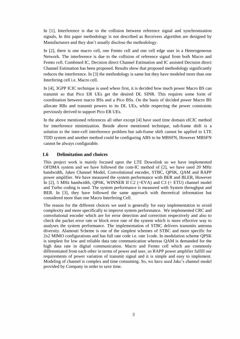
In LTE physical layer, Orthogonal Frequency Division Multiple Access (OFDMA) scheme is

used for downlink transmission. OFDMA make use of OFDM technology to multiplex

different users by assigning specific patterns of subcarriers in time and frequency domain. The

scheduling and assignment of resources makes OFDMA different from OFDM. In the OFDM

figure 2.4 shows that the entire bandwidth is assigned to single user for a certain period of

time but in OFDMA multiple users are sharing the bandwidth at each point in time [11].

8

Sub

Carr

iers

Time Time

OFDM OFDMA

Sub

Carr

iers

Figure 2.4: OFDM and OFDMA graphical concept

2.1.5 Spectrum flexibility in LTE

One of the main characteristics of LTE radio-access technology is Spectrum flexibility which

allows deployment of LTE radio-access in different frequency bands with different sizes since

spectrum has become a scarce resource. This flexibility includes 2 main areas as follows:

Flexibility in duplex arrangements

Bandwidth flexibility

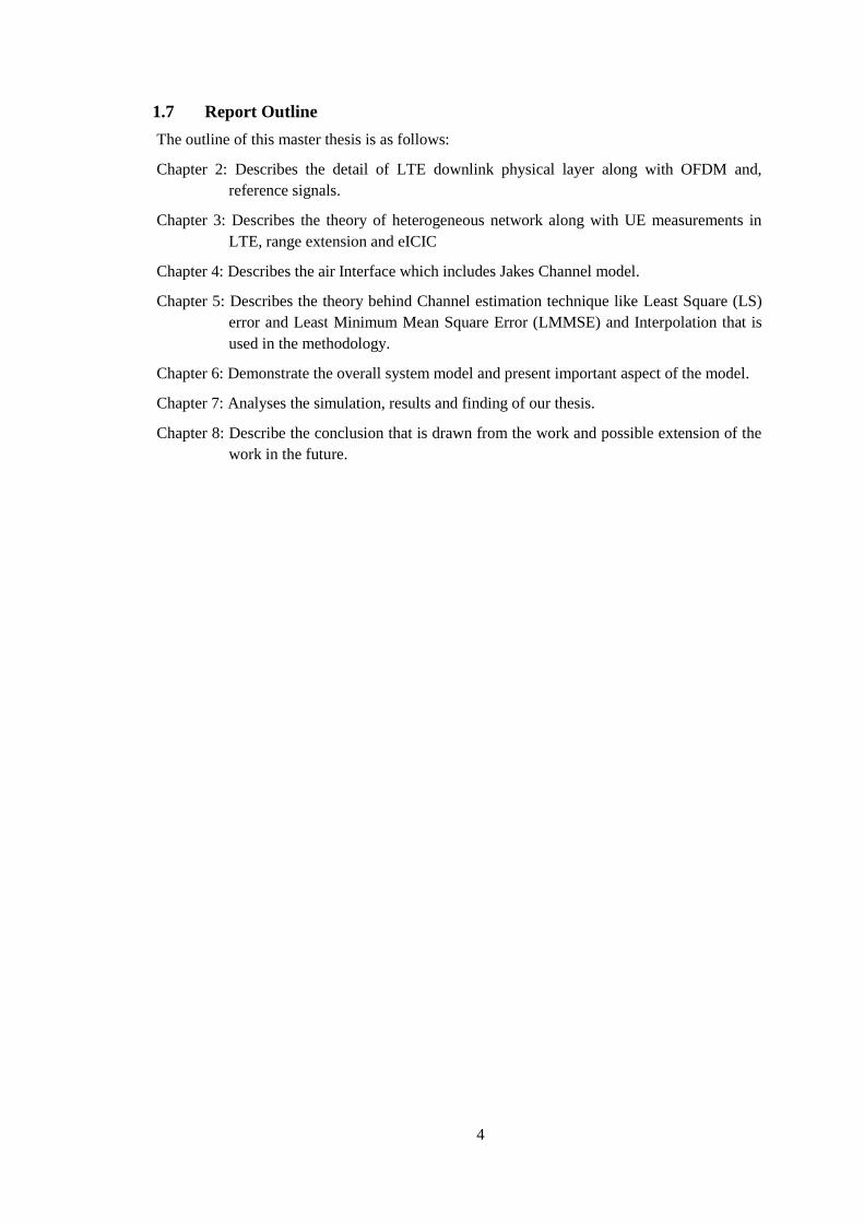
In Flexibility in duplex arrangements, the communication can take place both in paired and

unpaired bands. In former case the uplink and downlink transmissions use separate frequency

bands, while in later case downlink and uplink share the same frequency band. LTE support

both Frequency-Division Duplex (FDD) and Time-Division Duplex (TDD).

In FDD uplink and downlink transmissions take place in different and sufficiently separated

frequency bands, whereas in TDD uplink and downlink operate in different non-overlapping

time slots as shown in figure 2.5. In our thesis we have considered only FDD.

Time (t)Time (t)

Frequ

ency (f)

Frequ

ency (f)

F-DL

F-ULF-DL+ F-UL

FDD TDD

Figure 2.5: FDD and TDD

9

Bandwidth flexibility is an important aspect in the LTE operation. It is due to the fact that

LTE can be operated in different transmission bandwidths for uplink and downlink. The

reason for having different bandwidth is that LTE deployment depends upon the frequency

bands and on the operator. This bandwidth flexibility arise chances of gradual frequency

bands migration from other radio-access technologies.

2.1.6 LTE Generic Frame Structure

OFDMA is the best radio access for LTE downlink comparing to others. However, resource

allocation is complicated in OFDMA. It is far better than packet oriented approaches in the

context of efficiency and latency. In LTE, users are assigned a certain number of subcarriers

for predetermined period of time; these subcarriers are called physical resource blocks

(PRBs). These blocks have both time and frequency dimension [12].

Figure 2.6: LTE time domain frame structure.

As can be seen in the figure 2.6, LTE frame is of 10 millisecond ( ) duration which is

divided into 10 sub-frames of 1msec duration. Each sub-frame is further divided into two slots

each has a length of 0.5 . Each slot comprises either 6 or 7 OFDM symbols depending

upon normal or extended CP is used.

Table 2.1: LTE downlink Bandwidths

Bandwidth (MHz)

1.4

3

5.0

10.0

15.0

20.0

Subcarrier bandwidth (kHz)

15

Physical resource block (PRB)

bandwidth (kHz)

180

Number of available PRBs

6

12

25

50

75

100

10

Table 2.1 shows LTE specification defines different channel bandwidths from 1.4 to 20 .

Different channel bandwidth has different number of available PRBs. A PRB is comprises of

12 consecutive subcarriers for one slot as shown in figure 2.7 below. A PRB is the

smallest unit that base station can allocate to the user. Subcarrier bandwidth and PRBs

bandwidths are 15 and 180 respectively for all system bandwidths.

The figure 2.7 is shown for the case of normal CP. The transmitted downlink signal consists

of subcarriers for the duration of OFDM symbols.

1 Frame (10 msec)

1 Sub-Frame (1.0 msec)1 Slot (0.5 msec)

12

su

bca

rrie

rs

N s

ub

carr

iers

RESOURCE BLOCK7 symbols x 12 subcarriers (normal cp), or6 symbols x 12 subcarriers (extended cp)

Resource element

Time domain symbol

Fre

qu

en

cy d

om

ain

su

b-c

arr

iers

Figure 2.7: LTE time frequency resource grid

A Resource element is the smallest physical resource and it consists of one subcarrier during

one OFDM symbol. A group of resource elements are referred as physical resource blocks i.e.

PRBs. A PRB has a seven OFDM symbols having duration of one time slot 0.5ms and 12

subcarriers having a bandwidth of ( , so each resource

block in the case of normal cyclic prefix has of 84 resource elements (

) whereas in the case of extended cyclic prefix

resource block has 72 resource elements (

.

11

LTE downlink channel and signals 2.2

2.2.1 Downlink Reference Signals

Packet oriented networks use PHY preamble to facilitate carrier offset estimate, channel

estimation, timing synchronization etc. However, in LTE special reference signals are mapped

into the PRBs to allow coherent demodulation at the user equipment. Downlink reference

Signals are placed in the first and third last OFDM symbol in each slot. It means for the case

of normal CP reference signals are depicted in first and fifth OFDM symbol and of the

extended CP reference signals are depicted in first and fourth OFDM symbol. Frequency

spacing between two reference signals is six subcarriers. Therefore there are four reference

signals in one PRB. These reference signals are used to estimate the channel response on

subcarriers bearing them. Interpolation is employed to estimate the channel response on other

subcarriers [12]. Figure 2.8 given below illustrated are for single antenna LTE system with

normal CP.

0

1

2

3

4

6

7

8

9

10

1 2 3 4 5 6 0 1 2 3 4 5 6

R

R

R

R

R

R

R

R

Slot 0Subframe

12 S

ubca

rrie

rs

Slot 1

Figure 2.8: LTE CRSs Position in a single Antenna

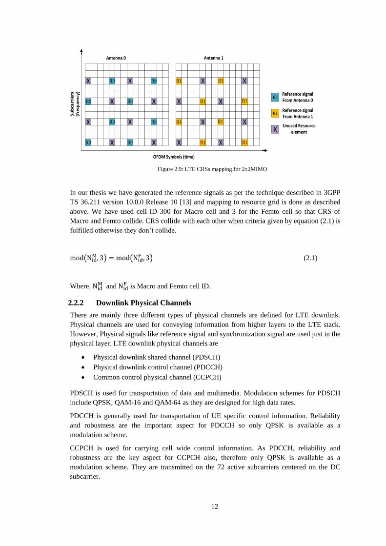
In the case of 2x2 MIMO operations, the receiver must determine channel impulse response

from each transmitting antenna. For the accurate channel estimation, when one antenna is

sending the reference signal other antenna does not transmit anything at the same time and

frequency position of reference signals. Mapping of reference signals for 2x2 MIMO

operations is shown in figure 2.9.

12

Reference signal From Antenna 0

Reference signal From Antenna 1

Unused Resource element

Su

bca

rrie

rs(f

req

ue

ncy

)

Antenna 0

OFDM Symbols (time)

Antenna 1

X

X

X

X

X

X

X

X

X

X

X

X

X

X

X

X

R1

R0

R0

R0

R0

R0

R0

R0

R0

R1

R1

R1 R1

R1

R1

R1

R0

R1

X

Figure 2.9: LTE CRSs mapping for 2x2MIMO

In our thesis we have generated the reference signals as per the technique described in 3GPP

TS 36.211 version 10.0.0 Release 10 [13] and mapping to resource grid is done as described

above. We have used cell ID 300 for Macro cell and 3 for the Femto cell so that CRS of

Macro and Femto collide. CRS collide with each other when criteria given by equation (2.1) is

fulfilled otherwise they don’t collide.

( ) (

) (2.1)

Where, and

is Macro and Femto cell ID.

2.2.2 Downlink Physical Channels

There are mainly three different types of physical channels are defined for LTE downlink.

Physical channels are used for conveying information from higher layers to the LTE stack.

However, Physical signals like reference signal and synchronization signal are used just in the

physical layer. LTE downlink physical channels are

Physical downlink shared channel (PDSCH)

Physical downlink control channel (PDCCH)

Common control physical channel (CCPCH)

PDSCH is used for transportation of data and multimedia. Modulation schemes for PDSCH

include QPSK, QAM-16 and QAM-64 as they are designed for high data rates.

PDCCH is generally used for transportation of UE specific control information. Reliability

and robustness are the important aspect for PDCCH so only QPSK is available as a

modulation scheme.

CCPCH is used for carrying cell wide control information. As PDCCH, reliability and

robustness are the key aspect for CCPCH also, therefore only QPSK is available as a

modulation scheme. They are transmitted on the 72 active subcarriers centered on the DC

subcarrier.

13

All the down link physical channels and signals and their specific mapping in LTE resource

grid for bandwidth 1.4MHz and 20MHz is shown in Appendix B.1 and B.2 respectively.

LTE-A Release 10 2.3

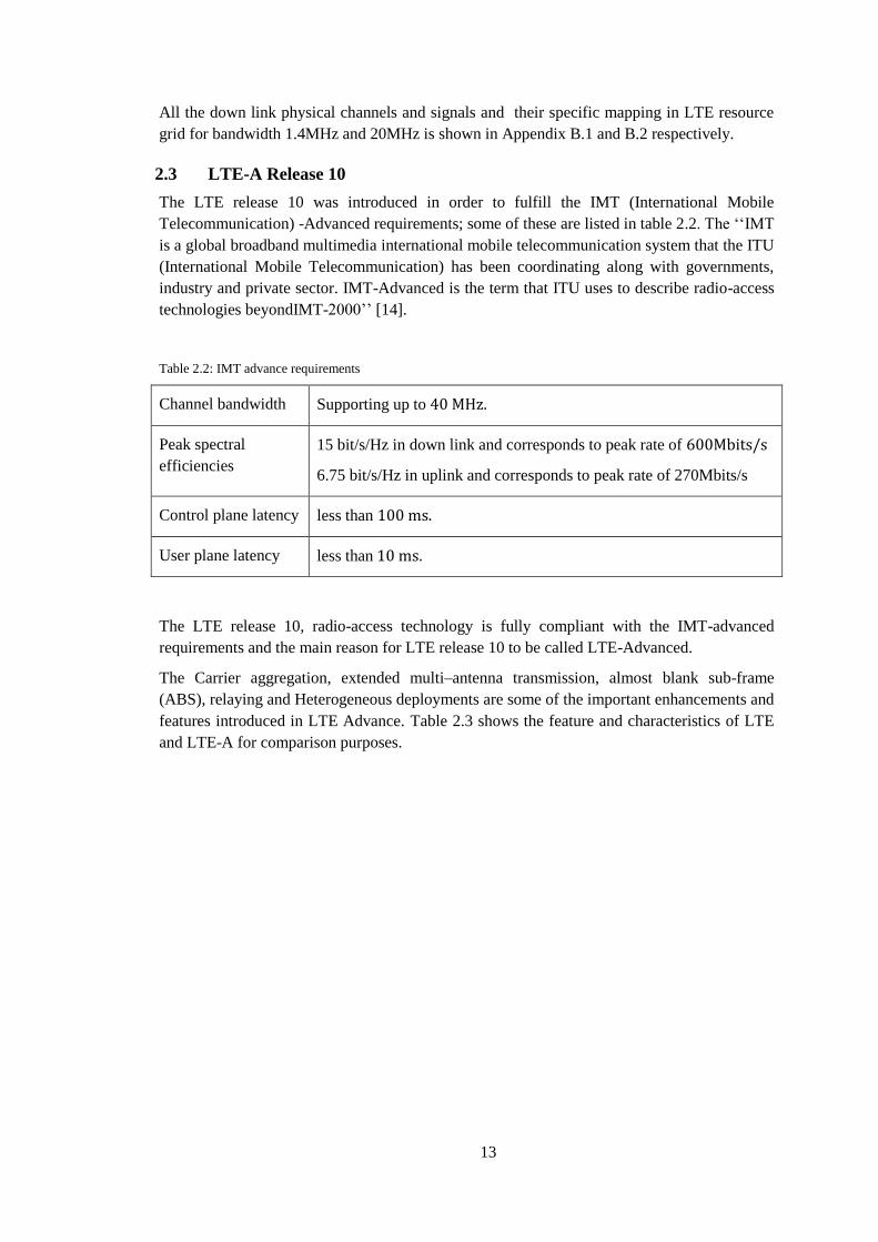
The LTE release 10 was introduced in order to fulfill the IMT (International Mobile

Telecommunication) -Advanced requirements; some of these are listed in table 2.2. The ‘‘IMT

is a global broadband multimedia international mobile telecommunication system that the ITU

(International Mobile Telecommunication) has been coordinating along with governments,

industry and private sector. IMT-Advanced is the term that ITU uses to describe radio-access

technologies beyondIMT-2000’’ [14].

Table 2.2: IMT advance requirements

Channel bandwidth Supporting up to

Peak spectral

efficiencies

15 bit/s/Hz in down link and corresponds to peak rate of

6.75 bit/s/Hz in uplink and corresponds to peak rate of 270Mbits/s

Control plane latency less than

User plane latency less than

The LTE release 10, radio-access technology is fully compliant with the IMT-advanced

requirements and the main reason for LTE release 10 to be called LTE-Advanced.

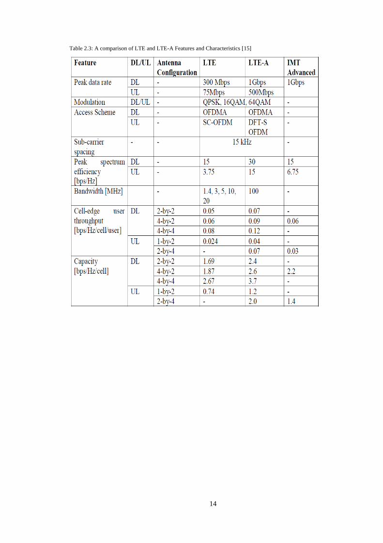
The Carrier aggregation, extended multi–antenna transmission, almost blank sub-frame

(ABS), relaying and Heterogeneous deployments are some of the important enhancements and

features introduced in LTE Advance. Table 2.3 shows the feature and characteristics of LTE

and LTE-A for comparison purposes.

14

Table 2.3: A comparison of LTE and LTE-A Features and Characteristics [15]

15

Chapter 3

Heterogeneous network

Introduction to heterogeneous network 3.1

Recently the number of mobile broadband users has been grown exponentially and it will

definitely grow more in the future. This is due to the fact that evolution on terminal

capabilities which can handle new and different kind of services. It is predicted that traffic per

year is going to be double in next five years, therefore by 2014 average traffic uses 1GB of

data per month compared to 100 or 200 MB now [16]

Scarcity of frequency spectrum is always a big issue. Spectral efficiency of wireless networks

is reaching its theoretical limits, it is necessary to increase the node density which can

improve the network capacity. If macro cell deployments are sparse then adding another cell

does not create significant inter-cell interference and cell splitting gain can be achieved.

However, if macro cells are already dense, cell splitting gains are significantly reduced

because of inter-cell interference. Instead of deploying macro cell another low power nodes

can be deployed. These low power nodes are called Pico cell and Femto cell. Those network

which consist of macro and low power nodes are called heterogeneous network [17]. In

heterogeneous network Pico/Femto cell with same set of frequencies are deployed within the

Macro cell in an unplanned way depending upon the areas that has more traffic. In one hand

these deployment increases the overall network capacity, data rate and the performance of the

cell-edge user and on the other hand such deployments cause severe Macro-Pico/Femto inter-

cell interference. Figure 3.1 shows the typical scenario of heterogeneous networks, where in

each cell there is one Macro base station, one Femto base station and one user equipment i.e.

UE.

Femto Base Station

Macro Base Station

UE

Figure 3.1: Heterogeneous Networks

In this thesis Femto cell and Pico cell are considered as same. Therefore we have taken Femto

cell that represents low power node (LPN). We have also considered the scenario where

Femto cell is deployed inside macro cell. In 3GPP LTE term base station is referred as

16

evolved node base station also abbreviated as eNBs for macro base station and HeNBs for

Femto base station.

3.1.1 Advantages of deployment of HeNBs

They can be deployed to eliminate coverage holes

Offer high data rate and capacity where they are deployed

less costly and easy to deploy comparing to macro cell

do not require air conditioning unit in the power amplifier

Cell splitting gain can be achieved

Traffic offloading to the low power nodes can be done

3.1.2 Properties of Macro eNBs and LPN

Macro eNBs

Power range around +45dBm

Covers outdoor with around cell site ~5km

Operator deployed

Femto eNBs

Power range around +15dBm

Covers indoor residence 50m

Operator deployed or User deployed

Equipped with Omnidirectional antenna

Backhaul uses the existing internet connection such as DSL

Pico Cell [17]

Power range around 23.97dBm for outdoor and 20dBm

Pico cell are regular macro cell except for low transmitting power

Equipped with Omnidirectional antenna

Backhaul uses the X2 interface for data communication and interference management

Relay [17]

Low power nodes (LPN) used in HetNets to enhance coverage.

No wired Backhaul ,wireless backhaul by relaying the signal from mobile station to

Macro eNB

In-band relay node uses the same UL and DL frequency where in out-of-band uses

different frequencies in UL and DL.

UE measurements in LTE 3.2

Reference signal received power (RSRP) is defined as the as the linear average over the power

contributions ( of the resource elements that carry cell-specific reference signals within

the considered measurement frequency bandwidth .For RSRP determination the cell-specific

reference signals (from first antenna) according to TS 36.211 [18] be used. If the UE can

reliably detect that (from second antenna) is available it may use in addition to to

determine RSRP [19].

17

Reference signal received quality (RSRQ) is defined as the ratio N×RSRP / (E-UTRA carrier

RSSI), where N is the number of RB’s of the E-UTRA carrier RSSI measurement bandwidth.

The measurements in the numerator and denominator shall be made over the same set of

resource blocks. E-UTRA Carrier Received Signal Strength Indicator (RSSI), comprises the

linear average of the total received power ( observed only in OFDM symbols containing

reference symbols for antenna port ‘0’, in the measurement bandwidth, over N number of

resource blocks by the UE from all sources, including co-channel serving and non-serving

cells, adjacent channel interference, thermal noise etc. [20].

Introduction to range extension 3.3

Cell selection in LTE is done based upon UE measurements of RSRP. In traditional Macro

cell networks the eNB having the high RSRP is selected [21]. However, in a heterogeneous

network there are base stations transmitting with different power level. So it is unfair to the

base station transmitting with lower power because terminal always chooses higher power

base station. This problem can be minimized if cell selection is done based upon uplink path

loss, which in practice is done by applying cell specific offset of the RSRP and RSRQ. This

method of cell selection increases the coverage area of the low power base station and this

increased area is named as range extension as shown in figure 3.2.

Range extension region

Figure 3.2: Range extension in Heterogeneous networks

Problem caused by deployment of Femto eNBs 3.4

As it is mentioned above that Femto eNBs which are also called HeNBs can be operator

deployed or user deployed. If it is operator deployed Macro user also have access to it which

is called open access but if it is user deployed Macro user cannot get connected to it only

limited number of users like family members of that particular home will have access to it

which is called closed subscriber group (CSG).

In this situation when Macro UE (user equipment) is in edge of Femto cell there will be strong

interference from Femto cell and may even not be able to access the Macro cell at all. In

another situation strong Macro cell interferes the Femto UE. This happens when sometime it

is preferable to connect UE to the Femto cell even if the received power from the Femto cell is

weaker than Macro cell. This is useful when strong cell has weak backhaul quality or when it

is necessary to offload the traffic to Femto cell and to achieve true cell-splitting gains in the

network [22].

Let’s take an example when UE is in cell extension region and it is connected to Femto base

station. But received power by the UE from the Macro is much higher than the power received

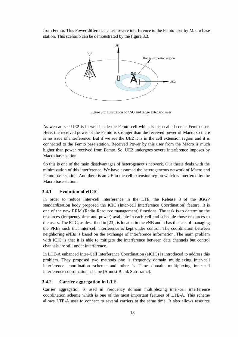
18

from Femto. This Power difference cause severe interference to the Femto user by Macro base

station. This scenario can be demonstrated by the figure 3.3.

Range extension region

UE1

UE2

Figure 3.3: Illustration of CSG and range extension user

As we can see UE2 is in well inside the Femto cell which is also called center Femto user.

Here, the received power of the Femto is stronger than the received power of Macro so there

is no issue of interference. But if we see the UE2 it is in the cell extension region and it is

connected to the Femto base station. Received Power by this user from the Macro is much

higher than power received from Femto. So, UE2 undergoes severe interference imposes by

Macro base station.

So this is one of the main disadvantages of heterogeneous network. Our thesis deals with the

minimization of this interference. We have assumed the heterogeneous network of Macro and

Femto base station. And there is an UE in the cell extension region which is interfered by the

Macro base station.

3.4.1 Evolution of eICIC

In order to reduce Inter-cell interference in the LTE, the Release 8 of the 3GGP

standardization body proposed the ICIC (Inter-cell Interference Coordination) feature. It is

one of the new RRM (Radio Resource management) functions. The task is to determine the

resources (frequency time and power) available in each cell and schedule those resources to

the users. The ICIC, as described in [23], is located in the eNB and it has the task of managing

the PRBs such that inter-cell interference is kept under control. The coordination between

neighboring eNBs is based on the exchange of interference information. The main problem

with ICIC is that it is able to mitigate the interference between data channels but control

channels are still under interference.

In LTE-A enhanced Inter-Cell Interference Coordination (eICIC) is introduced to address this

problem. They proposed two methods one is frequency domain multiplexing inter-cell

interference coordination scheme and other is Time domain multiplexing inter-cell

interference coordination scheme (Almost Blank Sub-frame).

3.4.2 Carrier aggregation in LTE

Carrier aggregation is used in Frequency domain multiplexing inter-cell interference

coordination scheme which is one of the most important features of LTE-A. This scheme

allows LTE-A user to connect to several carriers at the same time. It also allows resource

19

allocation across the carriers as well as fast switching between carriers without time

consuming handovers, which means a node, can schedule its control and data information on

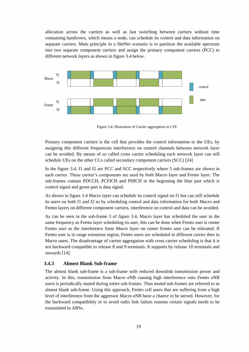
separate carriers. Main principle in a HetNet scenario is to partition the available spectrum

into two separate component carriers and assign the primary component carriers (PCC) to

different network layers as shown in figure 3.4 below.

control

data

f1

f2

f1

f2

Macro

Femto

Figure 3.4: Illustration of Carrier aggregation in LTE

Primary component carriers is the cell that provides the control information to the UEs, by

assigning this different frequencies interference on control channels between network layer

can be avoided. By means of so called cross carrier scheduling each network layer can still

schedule UEs on the other CCs called secondary component carriers (SCC) [24]

In the figure 3.4, f1 and f2 are PCC and SCC respectively where 5 sub-frames are shown in

each carrier. These carrier’s components are used by both Macro layer and Femto layer. The

sub-frames contain PDCCH, PCFICH and PHICH in the beginning the blue part which is

control signal and green part is data signal.

As shown in figure 3.4 Macro layer can schedule its control signal on f1 but can still schedule

its users on both f1 and f2 so by scheduling control and data information for both Macro and

Femto layers on different component carriers, interference on control and data can be avoided.

As can be seen in the sub-frame 3 of figure 3.4, Macro layer has scheduled the user in the

same frequency as Femto layer scheduling its user, this can be done when Femto user is center

Femto user as the interference from Macro layer on center Femto user can be tolerated. If

Femto user is in range extension region, Femto users are scheduled in different carrier then in

Macro users. The disadvantage of carrier aggregation with cross carrier scheduling is that it is

not backward compatible to release 8 and 9 terminals. It supports by release 10 terminals and

onwards [14].

3.4.3 Almost Blank Sub-frame

The almost blank sub-frame is a sub-frame with reduced downlink transmission power and

activity. In this, transmission from Macro eNB causing high interference onto Femto eNB

users is periodically muted during entire sub-frames. Thus muted sub-frames are referred to as

almost blank sub-frame. Using this approach, Femto cell users that are suffering from a high

level of interference from the aggressor Macro eNB have a chance to be served. However, for

the backward compatibility or to avoid radio link failure reasons certain signals needs to be

transmitted in ABSs.

20

Such signals are:

Cell specific reference signals (CRS) which are also called pilots

SIB-1 and paging with their associated PDCCH

Physical broadcast channel (PBCH)

Primary and secondary synchronization channels (PSS/SSS)

Collisions of sub-frame muting with PSS, SSS, SIB-1 and paging should be minimized. PSS,

SSS, SIB-1 and paging are transmitted in sub-frames #0, #1, #5 and #9.Without carefully

handling of these channels in the ABSs significant performance degradation can occur in

some situations.

ABSs muting patterns are configured semi-statically and signaled between eNBs over the X2

interface. These patterns are signaled in the form of bitmaps of length 40, i.e. spanning over 4

frames for FDD and 2 to 7 for TDD. Hence they can be configured dynamically by the

network.

controldata

Macro

Femto

ABS ABS

Rec

eiv

ed S

INR

fem

to u

ser

Time

Figure 3.5: Illustration of ABS in LTE

As shown in figure 3.5, Usage of ABS causes different level of interference between the sub-

frames of Macro and Femto. If Femto user is in range extension region and it is interfered by

strong Macro then Femto user can be served during the time when Macro transmit ABS else

Femto user can be served during ABS or non-ABS.

Colliding and Non colliding CRS 3.5

As it is explained earlier for the sake of backward compatibility and to avoid radio link failure

signals like CRSs, PCH, PBCH and PSS/SSS are still needs to be transmitted in the ABSs.

For simple study and investigation on the interference issue, we have considered a Macro cell

transmitting ABS with only CRS and a Femto is transmitting a sub-frame with PDSCH

channel and CRS. Since, the CRSs are spread all over the sub-frame in both in time and

frequency domain there is a chances that CRS of Femto sub-frame and CRS of ABS collide,

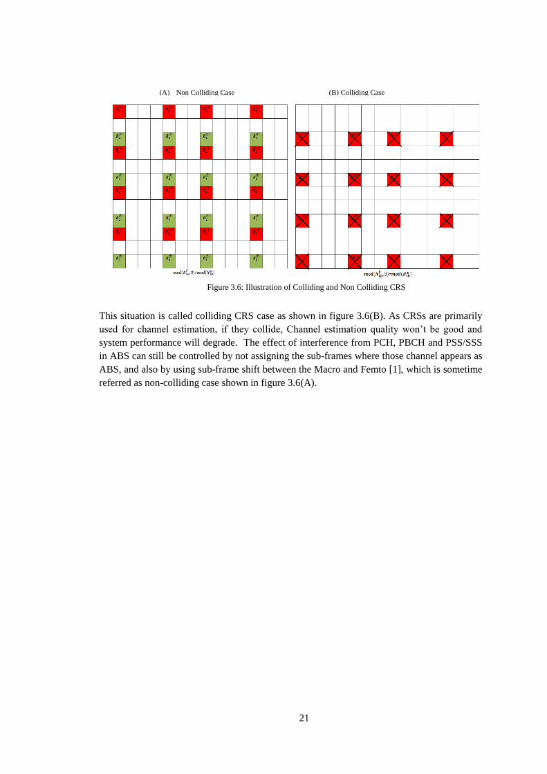
which is one of the worst scenarios encountered in the heterogeneous environment.

21

This situation is called colliding CRS case as shown in figure 3.6(B). As CRSs are primarily

used for channel estimation, if they collide, Channel estimation quality won’t be good and

system performance will degrade. The effect of interference from PCH, PBCH and PSS/SSS

in ABS can still be controlled by not assigning the sub-frames where those channel appears as

ABS, and also by using sub-frame shift between the Macro and Femto [1], which is sometime

referred as non-colliding case shown in figure 3.6(A).

(A) Non Colliding Case (B) Colliding Case

Figure 3.6: Illustration of Colliding and Non Colliding CRS

22

Chapter 4

Channel Model

Introduction to Air Interface 4.1

It is very important to have a good channel model for simulations as close to the reality as

possible. Correct channel models are also essential for testing, parameter optimization,

performance evaluation of communication systems and deployment of communication system

for reliable transfer of information between transmitter and receiver. On the basis of time,

channel may be time-invariant i.e. channel is constant over time or time-variant channel i.e.

channel varies over time. The time-invariant channels are relatively easy to estimate since it

only requires one estimate at the beginning of the reception of the signal whereas time-variant

channel is much harder to estimate since it requires continuous estimation.

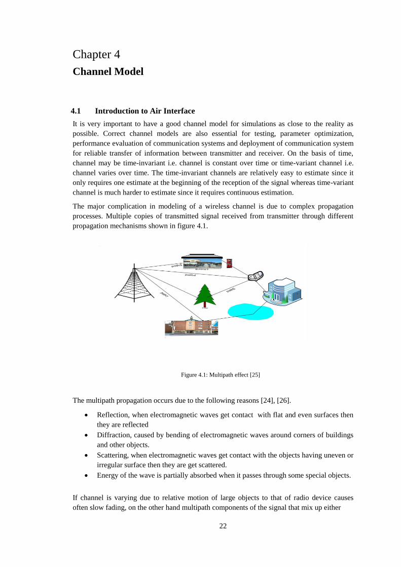
The major complication in modeling of a wireless channel is due to complex propagation

processes. Multiple copies of transmitted signal received from transmitter through different

propagation mechanisms shown in figure 4.1.

Figure 4.1: Multipath effect [25]

The multipath propagation occurs due to the following reasons [24], [26].

Reflection, when electromagnetic waves get contact with flat and even surfaces then

they are reflected

Diffraction, caused by bending of electromagnetic waves around corners of buildings

and other objects.

Scattering, when electromagnetic waves get contact with the objects having uneven or

irregular surface then they are get scattered.

Energy of the wave is partially absorbed when it passes through some special objects.

If channel is varying due to relative motion of large objects to that of radio device causes

often slow fading, on the other hand multipath components of the signal that mix up either

23

constructively or destructively causes fast fading. As a result of the terminal movements on

the order of half a wavelength a constructive superposition becomes destructive and vice

versa.

As shown from Figure 4.1 a receiver, receives multiple copies via different paths from

transmitter i.e. a multipath channel and is called as frequency selective channel hence, the

channel varies in frequency. On the other hand, when receiver receives only one copy of the

transmitted signal which results in a flat frequency fading, which in practice not the case

often. Instead the radio signal is reflected by objects before it reaches the receiver [8] and can

be modeled in time domain as

(4.1)

Where, and are stationary, statistically independent and real-valued Gaussian

processes and are typical not white processes, but instead colored Gaussian.

4.1.1 Rayleigh distributed channel

The central limits theorem will model the channel as a Rayleigh distributed channel, when

there are enough different paths, hence, and are Gaussian with zero-mean in

equation (4.1). The Equation (4.1) in polar form is given below

(4.2)

Where

√

(4.3)

And

(4.4)

This distribution represents the sum of amplitudes of the same order of a large number of

uncorrelated components with phases uniformly distributed in the interval (0, 2π). The

power delay profile (PDF) of Rayleigh distributed channel is described by equation below

(4.5)

24

Where, [ ] [

] and for < 0. The parameter is the root mean

square value of the received signal.

4.1.2 Rician distributed channel

In the presence of line of sight (LOS) component, the channel can be modeled as a Rician

distribution and is given by equation (4.6) as in [27].

(

)

(4.6)

Where modified Bassel function of first kind and Zero order and is the amplitude of the

line of sight component (LOS). In the absence of LOS component, Rician distribution can be

simply expressed as Rayleigh distribution. Since in this thesis MIMO is implemented and it is

assumed that there is no line of sight between the transmitter antennas and the receiver

antenna, so Rician distributed channel model is not our interest here.

4.1.3 Maximum Doppler shift

In statistical analysis of an extended Clarke’s model, the time varying nature of the wireless

channel is described by the wiener processes and where fixed Doppler shift through the multi-

path signal is introduced to describe the situation of a moving receiver and transmitter. A

closed-form expression for the autocorrelation function of the fading channel is derived which

contain a zero order Bessel function and decaying factor. The Bessel is the result of the

Doppler shift introduced due to the moving receiver and transmitter [28]. The maximum

Doppler shift is given by

(4.7)

Where is the Doppler shift, is the carrier frequency, is the relative velocity and is the

propagation speed of signal (speed of light) The above equation describes fast and slow fading

in batter way, since the receiver and transmitter moving relative to each other is the main

cause of fading.

Jake’s Channel model 4.2

In typical radio mobile communication scenario the transmitter is generally fixed whereas the

receiver is moving and reflection through objects produces a multi-path signal effect. The

direct LOS signal is not available in many cases and hence only signal reflected through

objects reach the moving receiver. The total received signal at moving receiver is well defined

by Jake’s model [29]. Equation (4.8) shows the impulse response of the channel;

∑ (4.8)

25

Where, is the delay of path and is the corresponding complex amplitude. Jakes

channel model does not take into consideration of the changing of delay paths M and the

delays over time. All is a complex Gaussian zero mean and can be defined as a

function of an angle and the distance between the receiver and the transmitter as

follows

∑ (4.9)

Zero order Bessel function, which depends upon the time difference and Doppler

shift, is the autocorrelation of the different transmission paths . The factor determines

the variation of the channel between successive symbols.

The way how the power is spread over the time is difficult to estimate for any channel model.

However, most simple type of power delay distribution is uniformly and exponentially. In

uniform distribution, power of the channel response is uniformly distributed over a certain

period of time, whereas exponential power delay distribution which is defined in [30] has

power distributed according to equation (4.10).

(4.10)

Where is an arbitrary constant and is the root mean-square delay spread of the channel.

The delays are all uniformly distributed over the delay time of the channel. Taking this in

to account the channel can now be defined as

∑ √

(4.11)

In the OFDM case different sub-carriers has different frequencies. Therefore it is important to

have time varying transfer function of the channel.

∫

∑ √ (4.12)

Above expression is the time varying transfer function of the channel which assumes that an

exponential power delay profile is used with set so that the average power is normalized to

one.

In this thesis, Jake’s channel model with an exponential power delay Profile is used to

generate time and frequency-variant channels as described in equation (4.12).

26

Chapter 5

Channel Estimation

Channel estimation 5.1

Channel estimation is an important part of receiver section. Without channel estimation the

received data in any receiver cannot be decoded correctly while propagated through time

varying environment (channel) or in other hand receiver have to use differential phase-shift

keying (DPSK), in the latter case signal-to-noise ratio (SNR) of 3-dB is less compared with

coherent phase-shift keying (PSK) [31]. For time varying channel, receiver must have a

continuous channel estimation and tracking. If it is not continuous then receiver performance

will degrade drastically.

In this thesis report two type of channel estimation i.e. LS and LMMSE are studied and

implemented. As in LTE, the CRSs are scattered in time frequency resource grid as describes

in LTE technical specification, 3GPP TS 36.211 [18] as shown in figure 2.8 and figure 2.9

for SISO and 2x2 MIMO respectively. Due to the scattered nature of CRSs in time frequency

resource grid, first channel is estimated at CRSs position using the received CRS and

Transmitted CRS by least squared estimate. While using frequency interpolation over the

estimate of CRS position, for the channel estimate of OFDM symbol having the CRS (OFDM

symbols #1, 4, 8 & 12 for 2x2 MIMO configurations). Finally channel is estimated over

OFDM symbol having no CRSs (OFDM symbols # 2, 3, 5, 6, 7, 9, 10, 11, 13, 14 for 2x2

MIMO configuration) using time interpolation on OFDM symbols having CRS.

Signal Model 5.2

In simulation work we use multi sub-frame to analyses the interference mitigation via

advanced interference cancelation schemes in LTE Down link system model. One LTE sub-

frame consists of 14 OFDM symbols as sown in figure 2.8. But for channel estimation of LTE

downlink we considered one OFDM symbol from single eNB in frequency domain and is

given by equation (5.1).

(5.1)

Where, is a frequency response vector of unknown channel to be estimated and having

the dimension of . is the diagonal matrix of transmitted data sample including

CRSs and Zeros and have the dimension of and is the AWGN noise.

The equation (5.1) in terms of channel impulse response (CIR) is given by equation (5.2) [32].

(5.2)

27

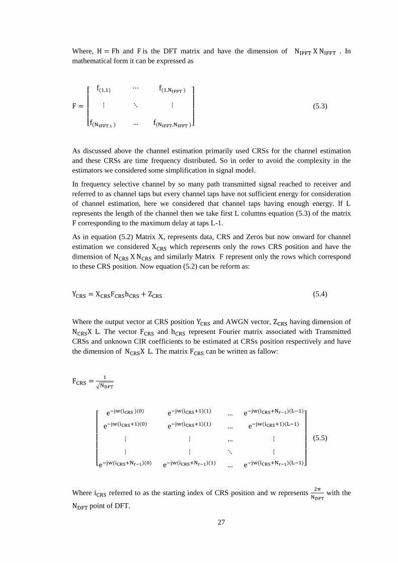
Where, and is the DFT matrix and have the dimension of . In

mathematical form it can be expressed as

[

]

(5.3)

As discussed above the channel estimation primarily used CRSs for the channel estimation

and these CRSs are time frequency distributed. So in order to avoid the complexity in the

estimators we considered some simplification in signal model.

In frequency selective channel by so many path transmitted signal reached to receiver and

referred to as channel taps but every channel taps have not sufficient energy for consideration

of channel estimation, here we considered that channel taps having enough energy. If L

represents the length of the channel then we take first L columns equation (5.3) of the matrix

F corresponding to the maximum delay at taps L-1.

As in equation (5.2) Matrix X, represents data, CRS and Zeros but now onward for channel

estimation we considered which represents only the rows CRS position and have the

dimension of and similarly Matrix F represent only the rows which correspond

to these CRS position. Now equation (5.2) can be reform as:

(5.4)

Where the output vector at CRS position and AWGN vector, having dimension of

. The vector and represent Fourier matrix associated with Transmitted

CRSs and unknown CIR coefficients to be estimated at CRSs position respectively and have

the dimension of . The matrix can be written as fallow:

√

[

]

(5.5)

Where referred to as the starting index of CRS position and represents

with the

point of DFT.

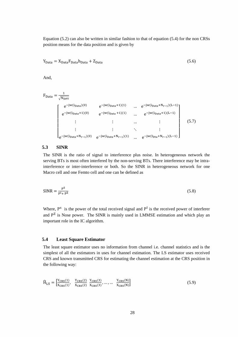
28

Equation (5.2) can also be written in similar fashion to that of equation (5.4) for the non CRSs

position means for the data position and is given by

(5.6)

And,

√

[

]

(5.7)

SINR 5.3

The SINR is the ratio of signal to interference plus noise. In heterogeneous network the

serving BTs is most often interfered by the non-serving BTs. There interference may be intra-

interference or inter-interference or both. So the SINR in heterogeneous network for one

Macro cell and one Femto cell and one can be defined as

(5.8)

Where, is the power of the total received signal and is the received power of interferer

and is Nose power. The SINR is mainly used in LMMSE estimation and which play an

important role in the IC algorithm.

Least Square Estimator 5.4

The least square estimator uses no information from channel i.e. channel statistics and is the

simplest of all the estimators in uses for channel estimation. The LS estimator uses received

CRS and known transmitted CRS for estimating the channel estimation at the CRS position in

the following way:

[

] (5.9)

29

Where is the estimated channel frequency response of the sub-carrier at the CRSs

position in OFDM symbol. The frequency and time interpolation is done according to section

5.1 to fully estimate the channel frequency response at the data position in OFDM symbols.

Due to low complexity the LS estimate is used widely but it has inherent disadvantage that it

has high mean square error. The LS channel estimation given in equation (5.9) is based on

minimization of the squared error without noise as described in [33], [34].

| | | |

| | (5.10)

After some mathematical calculation and by taking derivatives of squared error we get LS

estimation given bellow:

( )

( ) (5.11)

(5.12)

Where k = 1, 2, 3. . . N

Least Minimum Mean Square Error (LMMSE) Estimator 5.5

Least minimum mean squared error estimator is another type of 1D estimator, which gives the

estimate of channel impulse response (CIR) or channel frequency response (CFR) at the CRS

position in OFDM symbol. The LMMSE has advantage over the LS estimator that it gives

least mean square error means better performance as compared to LS, but the LMMSE

estimator has higher degree of computational complexity and also requires second order

channel statistics. The LMMSE performance criteria are based on the minimization of the

mean square error between the actual and estimated CIRs. These CFRs can be found while

using the LMMSE as describe in [32]. Now error is given by;

(5.12)

And

{ | | } { | | } { } (5.13)

Where in equation (5.13) { } is the expectation and channel AWGN noise assumed to be

uncorrelated, after some mathematical calculation we get

30

(5.14)

Where is the auto covariance matrix of and

is the cross covariance

matrix of the vector H and .

[

]

[ ]

[ (

)]

[ (

)]

[ ]

[

] (5.15)

In equation (5.15) (AWGN) noise and Channel frequency response H are uncorrelated so

their expectation value is Zero.

(5.16)

In equation (5.16) is the auto covariance matrix of

[

] (5.17)

[ ]

[ (

)]

[ ]

[

]

[ ] [

]

31

(5.18)

In equation (5.18) is the noise variance and is given by equation

{|

| } (5.19)

By using equations (5.11), (5.16) and (5.18) we can write the equation (5.14) for LMMSE as

below:

(

)

(5.20)

The above equation of justify the fact of computational complexity due to the

presence of term ( )

which is changes every time for the news input (next OFDM

symbol ) of in the case of CRS. This complexity in equation (5.20) can be reduced by

replacing complex matrix inversion by the expectation {( )

} . Then the above

equation (5.20) can be reformed as

(5.21)

Where is the modulation index and depends upon the constellation point which is

consequently directly depends on type of modulation scheme and code rate used. The value

for QPSK and QAM-16 are 1 and 17/9 respectively for the un-coded system which is

calculated as equation (5.22).

{ | | } { |

| } (5.22)

For the coded system the value depend upon the different code rate and modulation scheme

as given in table 5.1 [35].

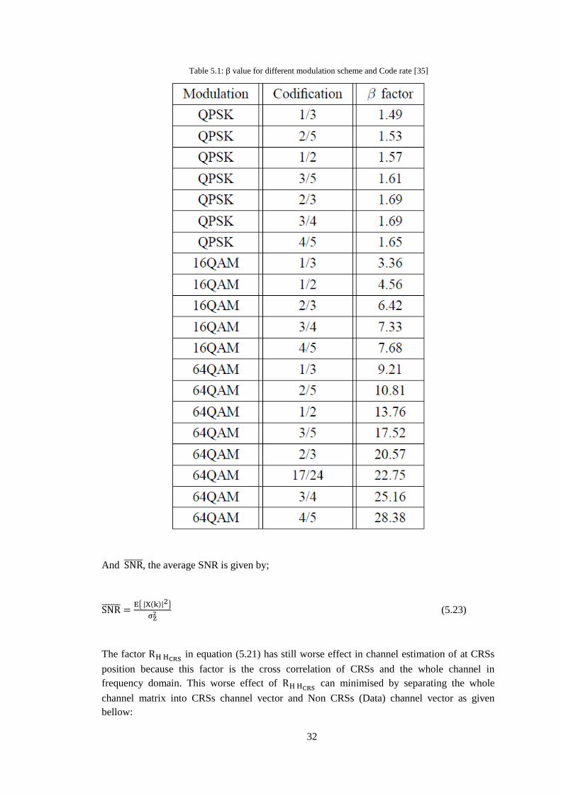
32

Table 5.1: value for different modulation scheme and Code rate [35]

And , the average SNR is given by;

{ | | }

(5.23)

The factor in equation (5.21) has still worse effect in channel estimation of at CRSs

position because this factor is the cross correlation of CRSs and the whole channel in

frequency domain. This worse effect of can minimised by separating the whole

channel matrix into CRSs channel vector and Non CRSs (Data) channel vector as given

bellow:

33

[

] (5.24)

Where are the CFRs at data position but not of CRSs position. By using equation (5.24)

in equation (5.21) estimation and interpolation can be split into two separate expressions as

given below:

(5.25)

(5.26)

Interpolation 5.6

In order to estimate the channel over data is necessary for achieving accuracy in demodulation

and good performance at receiver. In LTE downlink CRSs are time frequency distributed as

shown in figure 2.8 and figure 2.9. First frequency interpolation is needed in order to

optimally estimate the whole OFDM symbol containing CRSs and after that time interpolation

is done for other data OFDM downlink symbols on the basis of frequency interpolated OFDM

symbols.

5.6.1 Frequency Interpolation

There are different techniques for frequency interpolation in OFDM system as described in

[36]. In this thesis we used frequency interpolation for the OFDM symbols containing CRSs

and interpolates as whole symbol in frequency domain for the estimation CFRs at data

positions while using the estimated CFRSs of the equation (5.25) and is given by the equation

(

)

(5.27)

Instead of equation (5.27), equation (5.26) can also be used for the frequency interpolation.

The main difference between equation (5.26) and (5.27) is that the earlier equation estimate

the CFRs at the data position in OFDM symbols only whereas the later one estimated the

whole symbol.

5.6.2 Time Interpolation

As mention in section (5.1) the CFRS of the resource elements in OFDM symbols having no

CRSs can be determined by the time interpolation. On the bases of CFRS of the resource

elements in estimated OFDM symbols that are interpolated by frequency interpolation and

CFRs, the CFRs of the resource elements in non CRSs symbols are interpolated in time

domain by simple linear time interpolation to avoid the complexity. For time interpolation it is

assumed that OFDM symbols with in a sub-frame have strong correlation of the channel

frequency response. On the bases of previous and next OFDM symbol i.e. frequency

34

interpolated, the resource element of in the middle OFDM symbol can be interpolated as

follow [8].

(5.28)

Where and are the channel estimate of the previous and next

resource elements on the same carrier of frequency interpolated OFDM symbols (CRSs

OFDM symbols) respectively. Whereas and are the location or position of the

previous and next resource element on the same carrier from the respectively. As this

interpolation is based on the channel variation, which is directly related the channel coherence

time. In this thesis it assumed that the channel is constant within a resource block as mention

equation (6.26). Second in our simulation the channel model based on Jack’s channel model

criteria is not varying too much and the coherence time chosen is 0.01sec. Based on this

coherence time 138 OFDM symbol can be transmitted without degradation (One OFDM

symbol time is since one sub-frame time is 1 ).

Equalization 5.7

As the transmitted data passed through the time varying channel it convolve with the CIRs of

the channel due to which the received sub-carrier in OFDM data symbol suffer from distortion

in amplitudes and phase shift. So in order to compensate this distortion in amplitudes and

phase shift due to the multiplicative inverse of the complex channel equalization must be

performed. Two types of equalizations are described in [25] that are:

Time domain equalization

Frequency domain equalization

CP RemovalSub-CarrierDe-Mapping

N-Point DFT

Time Domain EqualizationFrequency Domain

Equalization

. . .

. . .

Figure 5.1: LTE time domain and frequency domain equalizer option

Time domain equalization is done on data symbols in time domain in order to equalize it with

the transmitted data symbol as show in figure 5.1. The time domain equalization is used in

OFDM receiver where the performances of the other equalizer are not important as in time

varying propagation condition.

Frequency domain equalization try to reduce the error between receive sub-carrier of OFDM

data symbol and transmitted OFDM data symbol in frequency domain. In frequency domain

equalization, received time domain OFDM data symbols are first transformed into frequency

35

domain while using N- point DFT and then equalization is done by frequency domain

filtering.

In simulation we performed the frequency domain equalization and the frequency domain

system model of equation (5.6) can be written as for the data sub-carrier as

(5.29)

Where is the resource element of the . The equalized output can be

writing as below

‖ ‖

(5.30)

36

Chapter 6

System Model

Introduction to System Model 6.1

Since we have considered Heterogeneous Network with Macro and Femto cell and Femto cell

UE in the cell extension region, we have modeled two transmitter base station one for Macro

as interferer cell and Femto as serving cell and one receivers.

We have mentioned in the methodology that Macro transmits ABS with CRS. For the

simplicity, we have shown general transmitter model for both Macro and Femto. It starts with

the generation of data bits. Now onwards we have described the model with block by block

basis. Close pictorial image of the system model is shown in figure 6.1.

Channel estimation

Tx CRS

Receiver

Bit genertaion CRC

Convolencoding

Ant 1

Ant 2

Ant 1

CRS genertaion

Modulation(QPSK,QAM)

Femto Transmitter(Serving HeNB)

STBC

Ant 2

Maping

Ant 1

Ant 2

FFT

Ant 1

Ant 2

CP Insertion

Ant 1

Ant 2

PA

Channel (Air interface)

Bit genertaion

CRCConvolencodin

g

Ant 1

Ant 2

Ant 1

CRS genertaion

Modulation(QPSK,QAM)

STBC

Ant 2

Maping

Ant 1

Ant 2

FFT

Ant 1

Ant 2

CP Insertion

Ant 1

Ant 2

PA

Macro Transmitter(Interfering eNB)

Ant 1

Ant 2

STBC

Extraction

Ant 1

Ant 2

IFFT

Ant 1

Ant 2

CP Removal

Ant 1

Ant 2

AWGN

RX Data CRC Check

Viterbi

DeModulation

(QPSK,QAM)Rx Data

Rx CRS

Equilization

Femto Ant 1

Femto Ant 2

Macro Ant 1

Macro Ant 2

RX Ant 1

RX Ant 2

Encoder

Encoder

Decoder

Figure 6.1: System model

Encoder 6.2

At first, 24 bits CRC is appended at the end of the generated bit, the output is called ‘code

word’. The code word is then passed through the convolutional encoder of code rate 1/3.

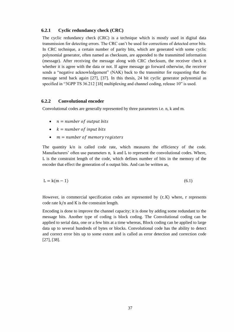
37

6.2.1 Cyclic redundancy check (CRC)

The cyclic redundancy check (CRC) is a technique which is mostly used in digital data

transmission for detecting errors. The CRC can’t be used for corrections of detected error bits.

In CRC technique, a certain number of parity bits, which are generated with some cyclic

polynomial generator, often named as checksum, are appended to the transmitted information

(message). After receiving the message along with CRC checksum, the receiver check it

whether it is agree with the data or not. If agree message go forward otherwise, the receiver

sends a “negative acknowledgement” (NAK) back to the transmitter for requesting that the

message send back again [27], [37]. In this thesis, 24 bit cyclic generator polynomial as

specified in “3GPP TS 36.212 [18] multiplexing and channel coding, release 10” is used.

6.2.2 Convolutional encoder

Convolutional codes are generally represented by three parameters i.e. n, k and m.

The quantity k/n is called code rate, which measures the efficiency of the code.

Manufacturers’ often use parameters and to represent the convolutional codes. Where,

is the constraint length of the code, which defines number of bits in the memory of the

encoder that effect the generation of n output bits. And can be written as,

(6.1)

However, in commercial specification codes are represented by where, represents

code rate and is the constraint length.

Encoding is done to improve the channel capacity; it is done by adding some redundant to the

message bits. Another type of coding is block coding. The Convolutional coding can be

applied to serial data, one or a few bits at a time whereas, Block coding can be applied to large

data up to several hundreds of bytes or blocks. Convolutional code has the ability to detect

and correct error bits up to some extent and is called as error detection and correction code

[27], [38].

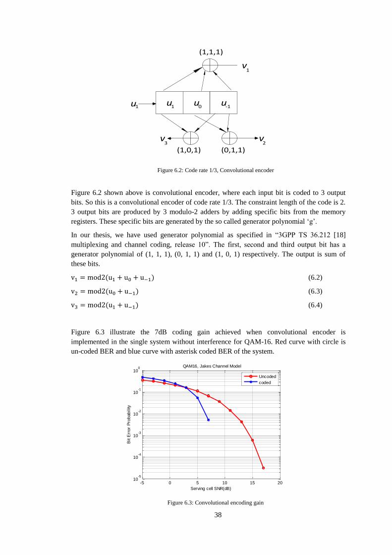
38

u u u-11 01

v

v

1

2v

3

(1,1,1)

(0,1,1)(1,0,1)

u

Figure 6.2: Code rate 1/3, Convolutional encoder

Figure 6.2 shown above is convolutional encoder, where each input bit is coded to 3 output

bits. So this is a convolutional encoder of code rate 1/3. The constraint length of the code is 2.

3 output bits are produced by 3 modulo-2 adders by adding specific bits from the memory

registers. These specific bits are generated by the so called generator polynomial ‘g’.

In our thesis, we have used generator polynomial as specified in “3GPP TS 36.212 [18]

multiplexing and channel coding, release 10”. The first, second and third output bit has a

generator polynomial of (1, 1, 1), (0, 1, 1) and (1, 0, 1) respectively. The output is sum of

these bits.

(6.2)

(6.3)

(6.4)

Figure 6.3 illustrate the 7dB coding gain achieved when convolutional encoder is

implemented in the single system without interference for QAM-16. Red curve with circle is

un-coded BER and blue curve with asterisk coded BER of the system.

Figure 6.3: Convolutional encoding gain

-5 0 5 10 15 2010

-5

10-4

10-3

10-2

10-1

100 QAM16, Jakes Channel Model

Serving cell SNR(dB)

Bit E

rro

r P

rob

ab

ility

Uncoded

coded

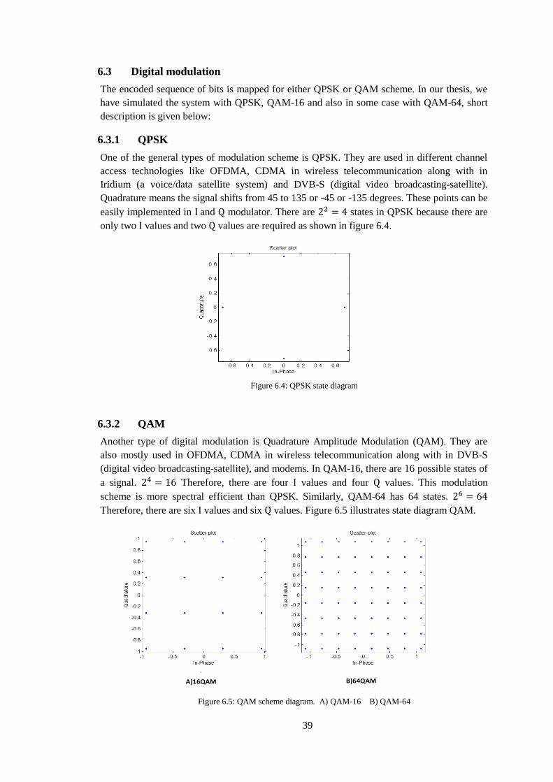
39

Digital modulation 6.3

The encoded sequence of bits is mapped for either QPSK or QAM scheme. In our thesis, we

have simulated the system with QPSK, QAM-16 and also in some case with QAM-64, short

description is given below:

6.3.1 QPSK

One of the general types of modulation scheme is QPSK. They are used in different channel

access technologies like OFDMA, CDMA in wireless telecommunication along with in

Iridium (a voice/data satellite system) and DVB-S (digital video broadcasting-satellite).

Quadrature means the signal shifts from 45 to 135 or -45 or -135 degrees. These points can be

easily implemented in and modulator. There are states in QPSK because there are

only two values and two values are required as shown in figure 6.4.

Figure 6.4: QPSK state diagram

6.3.2 QAM

Another type of digital modulation is Quadrature Amplitude Modulation (QAM). They are

also mostly used in OFDMA, CDMA in wireless telecommunication along with in DVB-S

(digital video broadcasting-satellite), and modems. In QAM-16, there are 16 possible states of

a signal. Therefore, there are four values and four values. This modulation

scheme is more spectral efficient than QPSK. Similarly, QAM-64 has 64 states.

Therefore, there are six values and six values. Figure 6.5 illustrates state diagram QAM.

B)64QAMA)16QAM

Figure 6.5: QAM scheme diagram. A) QAM-16 B) QAM-64

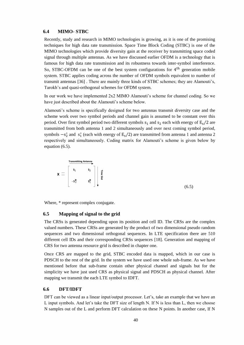
40

MIMO- STBC 6.4

Recently, study and research in MIMO technologies is growing, as it is one of the promising

techniques for high data rate transmission. Space Time Block Coding (STBC) is one of the

MIMO technologies which provide diversity gain at the receiver by transmitting space coded

signal through multiple antennas. As we have discussed earlier OFDM is a technology that is

famous for high data rate transmission and its robustness towards inter-symbol interference.

So, STBC-OFDM can be one of the best system configurations for generation mobile

system. STBC applies coding across the number of OFDM symbols equivalent to number of

transmit antennas [36] . There are mainly three kinds of STBC schemes; they are Alamouti’s,

Tarokh’s and quasi-orthogonal schemes for OFDM system.

In our work we have implemented 2x2 MIMO Alamouti’s scheme for channel coding. So we

have just described about the Alamouti’s scheme below.

Alamouti’s scheme is specifically designed for two antennas transmit diversity case and the

scheme work over two symbol periods and channel gain is assumed to be constant over this

period. Over first symbol period two different symbols and each with energy of are

transmitted from both antenna 1 and 2 simultaneously and over next coming symbol period,

symbols and

(each with energy of ) are transmitted from antenna 1 and antenna 2

respectively and simultaneously. Coding matrix for Alamouti’s scheme is given below by

equation (6.5).

S*1

S2

- S*2

S1

Transmitting Antenna

Time

Slot

X

(6.5)

Where, * represent complex conjugate.

Mapping of signal to the grid 6.5

The CRSs is generated depending upon its position and cell ID. The CRSs are the complex

valued numbers. These CRSs are generated by the product of two dimensional pseudo random

sequences and two dimensional orthogonal sequences. In LTE specification there are 510

different cell IDs and their corresponding CRSs sequences [18]. Generation and mapping of

CRS for two antenna resource grid is described in chapter one.

Once CRS are mapped to the grid, STBC encoded data is mapped, which in our case is

PDSCH to the rest of the grid. In the system we have used one whole sub-frame. As we have

mentioned before that sub-frame contain other physical channel and signals but for the

simplicity we have just used CRS as physical signal and PDSCH as physical channel. After

mapping we transmit the each LTE symbol to IDFT.

DFT/IDFT 6.6

DFT can be viewed as a linear input/output processor. Let’s, take an example that we have an

L input symbols. And let’s take the DFT size of length N. If N is less than L, then we choose

N samples out of the L and perform DFT calculation on these N points. In another case, If N

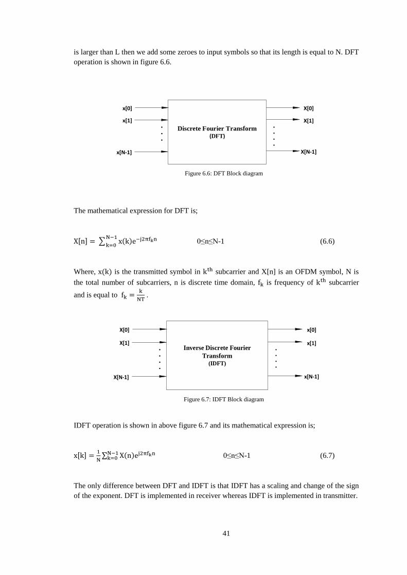
41

is larger than L then we add some zeroes to input symbols so that its length is equal to N. DFT

operation is shown in figure 6.6.

Discrete Fourier Transform(DFT)

x[0]

x[1]

x[N-1]

X[0]

X[1]

X[N-1]

Figure 6.6: DFT Block diagram

The mathematical expression for DFT is;

[ ] ∑

0≤n≤N-1 (6.6)

Where, is the transmitted symbol in subcarrier and X[n] is an OFDM symbol, N is

the total number of subcarriers, n is discrete time domain, is frequency of subcarrier

and is equal to

.

Inverse Discrete Fourier

Transform(IDFT)

X[0]

X[1]

X[N-1]

x[0]

x[1]

x[N-1]

Figure 6.7: IDFT Block diagram

IDFT operation is shown in above figure 6.7 and its mathematical expression is;

[ ]

∑

0≤n≤N-1 (6.7)

The only difference between DFT and IDFT is that IDFT has a scaling and change of the sign

of the exponent. DFT is implemented in receiver whereas IDFT is implemented in transmitter.

42

Cyclic Prefix (CP) 6.7

After IFFT, CP is added to the signal. Detail description of CP is done in section 2.1.4

Power Amplifier 6.8

The power amplifier is used to boost up the radio frequency to achieve desired power level for

the transmission on air interface. In our case, there is Heterogeneous Network i.e. Macro-eNB

and Femto-HeNB, both operates at different power level.

A baseband equivalent nonlinearity characterized by AM/AM (amplitude to amplitude) and

AM/PM (amplitude to phase) mapping is illustrated in figure 6.8 where the notation and

are actually functions operating on amplitude of the base band signal [39].

Figure 6.8: AM/AM & AM/PM mapping

Where,

(6.8)

( ) (6.9)

In our simulation, we have used Rapp Power Amplifier Model which is also named as the

Solid state power amplifiers (SSPA). This is more linear to small signal as compared to the

Traveling Wave Tube Amplifiers (TWTA) and clipping for large signals. The characteristics

of the Rapp model is given by equation (6.10) [39].

⌊ (

)

⌋ (6.10)

(6.11)

Where and are the mapping from the amplitude and phase of the base band

input to amplitude and phase of the base band output respectively, k is the small gain, is

𝑔𝐴 𝑔 𝐺 𝑥 𝑡

𝑥 𝑡 𝑦 𝑡

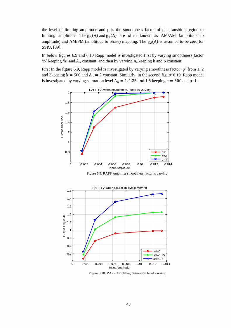
43

the level of limiting amplitude and p is the smoothness factor of the transition region to

limiting amplitude. The and are often known as AM/AM (amplitude to

amplitude) and AM/PM (amplitude to phase) mapping. The is assumed to be zero for

SSPA [39].

In below figures 6.9 and 6.10 Rapp model is investigated first by varying smoothness factor

‘ ’ keeping ‘ ’ and constant, and then by varying keeping and constant.

First In the figure 6.9, Rapp model is investigated by varying smoothness factor ‘ ’ from 1, 2

and 3keeping 500 and constant. Similarly, in the second figure 6.10, Rapp model

is investigated by varying saturation level keeping and p=1.

Figure 6.9: RAPP Amplifier smoothness factor is varying

Figure 6.10: RAPP Amplifier, Saturation level varying

0 0.002 0.004 0.006 0.008 0.01 0.012 0.014

0.8

1

1.2

1.4

1.6

1.8

2RAPP PA when smoothness factor is varying

Input Amplitude

Out

pu

t A

mp

litud

e

p=1

p=2

p=3

0 0.002 0.004 0.006 0.008 0.01 0.012 0.014

0.7

0.8

0.9

1

1.1

1.2

1.3

1.4

1.5RAPP PA when saturation level is varying

Input Amplitude

Outp

ut

Am

plitu

de

sat=1

sat=1.25

sat=1.5

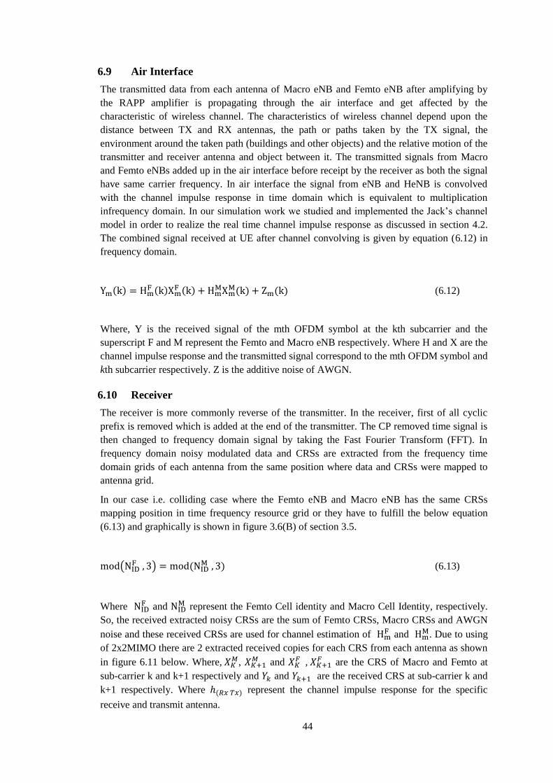
44

Air Interface 6.9

The transmitted data from each antenna of Macro eNB and Femto eNB after amplifying by

the RAPP amplifier is propagating through the air interface and get affected by the

characteristic of wireless channel. The characteristics of wireless channel depend upon the

distance between TX and RX antennas, the path or paths taken by the TX signal, the

environment around the taken path (buildings and other objects) and the relative motion of the

transmitter and receiver antenna and object between it. The transmitted signals from Macro

and Femto eNBs added up in the air interface before receipt by the receiver as both the signal

have same carrier frequency. In air interface the signal from eNB and HeNB is convolved

with the channel impulse response in time domain which is equivalent to multiplication

infrequency domain. In our simulation work we studied and implemented the Jack’s channel

model in order to realize the real time channel impulse response as discussed in section 4.2.

The combined signal received at UE after channel convolving is given by equation (6.12) in

frequency domain.

(6.12)

Where, Y is the received signal of the mth OFDM symbol at the kth subcarrier and the

superscript F and M represent the Femto and Macro eNB respectively. Where H and X are the

channel impulse response and the transmitted signal correspond to the mth OFDM symbol and

kth subcarrier respectively. Z is the additive noise of AWGN.

Receiver 6.10

The receiver is more commonly reverse of the transmitter. In the receiver, first of all cyclic

prefix is removed which is added at the end of the transmitter. The CP removed time signal is

then changed to frequency domain signal by taking the Fast Fourier Transform (FFT). In

frequency domain noisy modulated data and CRSs are extracted from the frequency time

domain grids of each antenna from the same position where data and CRSs were mapped to

antenna grid.

In our case i.e. colliding case where the Femto eNB and Macro eNB has the same CRSs

mapping position in time frequency resource grid or they have to fulfill the below equation

(6.13) and graphically is shown in figure 3.6(B) of section 3.5.

( )

(6.13)

Where and

represent the Femto Cell identity and Macro Cell Identity, respectively.

So, the received extracted noisy CRSs are the sum of Femto CRSs, Macro CRSs and AWGN

noise and these received CRSs are used for channel estimation of and

. Due to using

of 2x2MIMO there are 2 extracted received copies for each CRS from each antenna as shown

in figure 6.11 below. Where, ,

and ,

are the CRS of Macro and Femto at

sub-carrier k and k+1 respectively and and are the received CRS at sub-carrier k and

k+1 respectively. Where represent the channel impulse response for the specific

receive and transmit antenna.

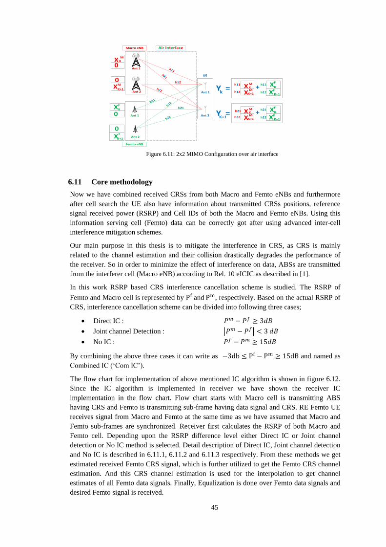
45

K+1

K+1

Macro eNB

Femto eNB

Ant 2

Ant 1

Ant 1

Ant 2

UE

Ant 1

Ant 2

h12

h21

0XM

XF

0

Y =k

Y =K+1

h11 h11+

X0

F

K

XF

K

X0

MK

X MK

XM

K+1h12 XF

K+1h12

h21+ XF

KX MK

XM

K+1h22 XF

K+1h22

h21

Air Interface

Figure 6.11: 2x2 MIMO Configuration over air interface

Core methodology 6.11

Now we have combined received CRSs from both Macro and Femto eNBs and furthermore

after cell search the UE also have information about transmitted CRSs positions, reference

signal received power (RSRP) and Cell IDs of both the Macro and Femto eNBs. Using this

information serving cell (Femto) data can be correctly got after using advanced inter-cell

interference mitigation schemes.

Our main purpose in this thesis is to mitigate the interference in CRS, as CRS is mainly

related to the channel estimation and their collision drastically degrades the performance of

the receiver. So in order to minimize the effect of interference on data, ABSs are transmitted

from the interferer cell (Macro eNB) according to Rel. 10 eICIC as described in [1].

In this work RSRP based CRS interference cancellation scheme is studied. The RSRP of

Femto and Macro cell is represented by and , respectively. Based on the actual RSRP of

CRS, interference cancellation scheme can be divided into following three cases;

Direct IC :

Joint channel Detection : | |

No IC :

By combining the above three cases it can write as and named as

Combined IC (‘Com IC’).

The flow chart for implementation of above mentioned IC algorithm is shown in figure 6.12.

Since the IC algorithm is implemented in receiver we have shown the receiver IC

implementation in the flow chart. Flow chart starts with Macro cell is transmitting ABS

having CRS and Femto is transmitting sub-frame having data signal and CRS. RE Femto UE

receives signal from Macro and Femto at the same time as we have assumed that Macro and

Femto sub-frames are synchronized. Receiver first calculates the RSRP of both Macro and

Femto cell. Depending upon the RSRP difference level either Direct IC or Joint channel

detection or No IC method is selected. Detail description of Direct IC, Joint channel detection

and No IC is described in 6.11.1, 6.11.2 and 6.11.3 respectively. From these methods we get

estimated received Femto CRS signal, which is further utilized to get the Femto CRS channel

estimation. And this CRS channel estimation is used for the interpolation to get channel

estimates of all Femto data signals. Finally, Equalization is done over Femto data signals and

desired Femto signal is received.

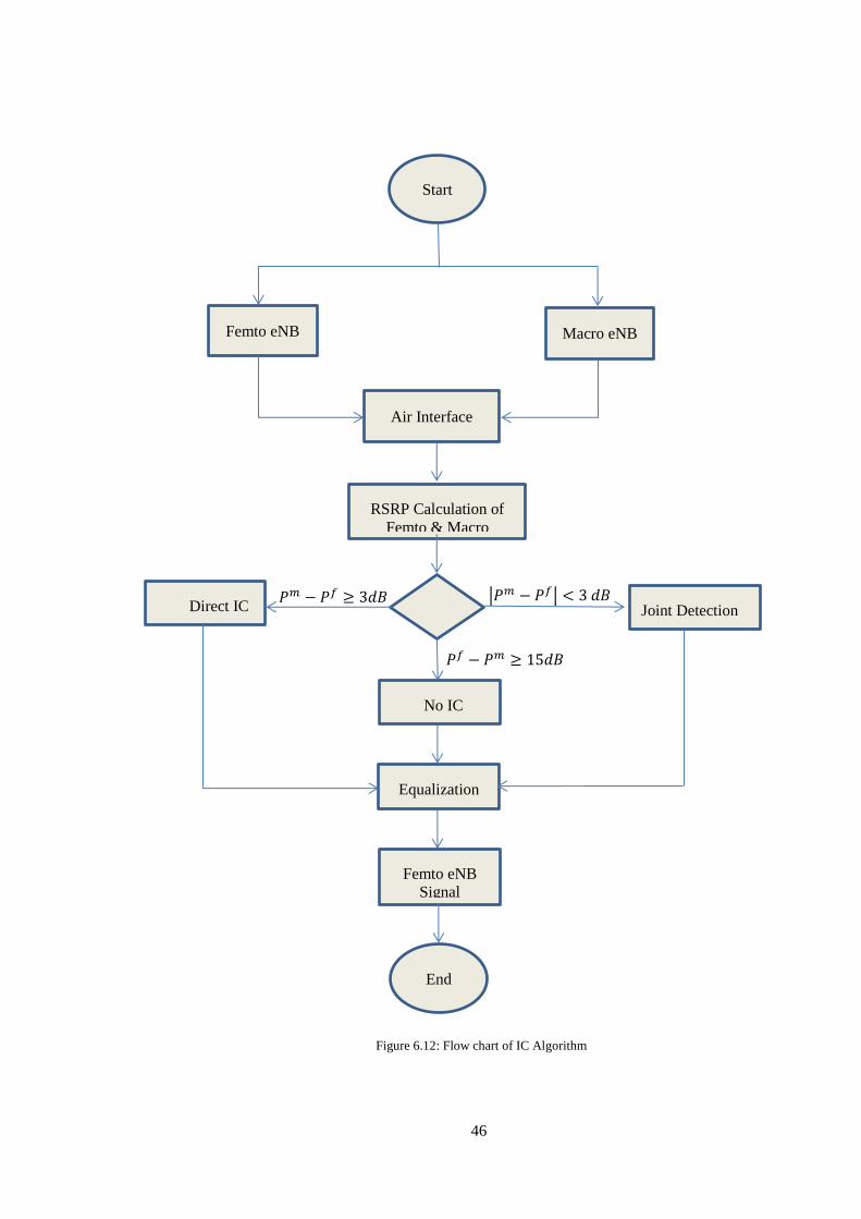
46

Femto eNB Macro eNB

Air Interface

Start

𝑃𝑓 𝑃𝑚 𝑑𝐵

|𝑃𝑚 𝑃𝑓| 𝑑𝐵 𝑃𝑚 𝑃𝑓 𝑑𝐵

RSRP Calculation of

Femto & Macro

Direct IC Joint Detection

No IC

End

Equalization

Femto eNB

Signal

Detection

Figure 6.12: Flow chart of IC Algorithm

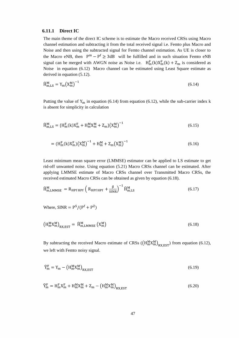
47

6.11.1 Direct IC

The main theme of the direct IC scheme is to estimate the Macro received CRSs using Macro

channel estimation and subtracting it from the total received signal i.e. Femto plus Macro and

Noise and then using the subtracted signal for Femto channel estimation. As UE is closer to

the Macro eNB, then will be fulfilled and in such situation Femto eNB

signal can be merged with AWGN noise as Noise i.e.

is considered as

Noise in equation (6.12) Macro channel can be estimated using Least Square estimate as

derived in equation (5.12).

(

)

(6.14)

Putting the value of in equation (6.14) from equation (6.12), while the sub-carrier index k

is absent for simplicity in calculation

{

}(

)

(6.15)

( )

( )

(6.16)

Least minimum mean square error (LMMSE) estimator can be applied to LS estimate to get

rid-off unwanted noise. Using equation (5.21) Macro CRSs channel can be estimated. After

applying LMMSE estimate of Macro CRSs channel over Transmitted Macro CRSs, the

received estimated Macro CRSs can be obtained as given by equation (6.18).

(

)

(6.17)

Where,

(

)

(

) (6.18)

By subtracting the received Macro estimate of CRSs ((

)

) from equation (6.12),

we left with Femto noisy signal.

(

)

(6.19)

(

)

(6.20)

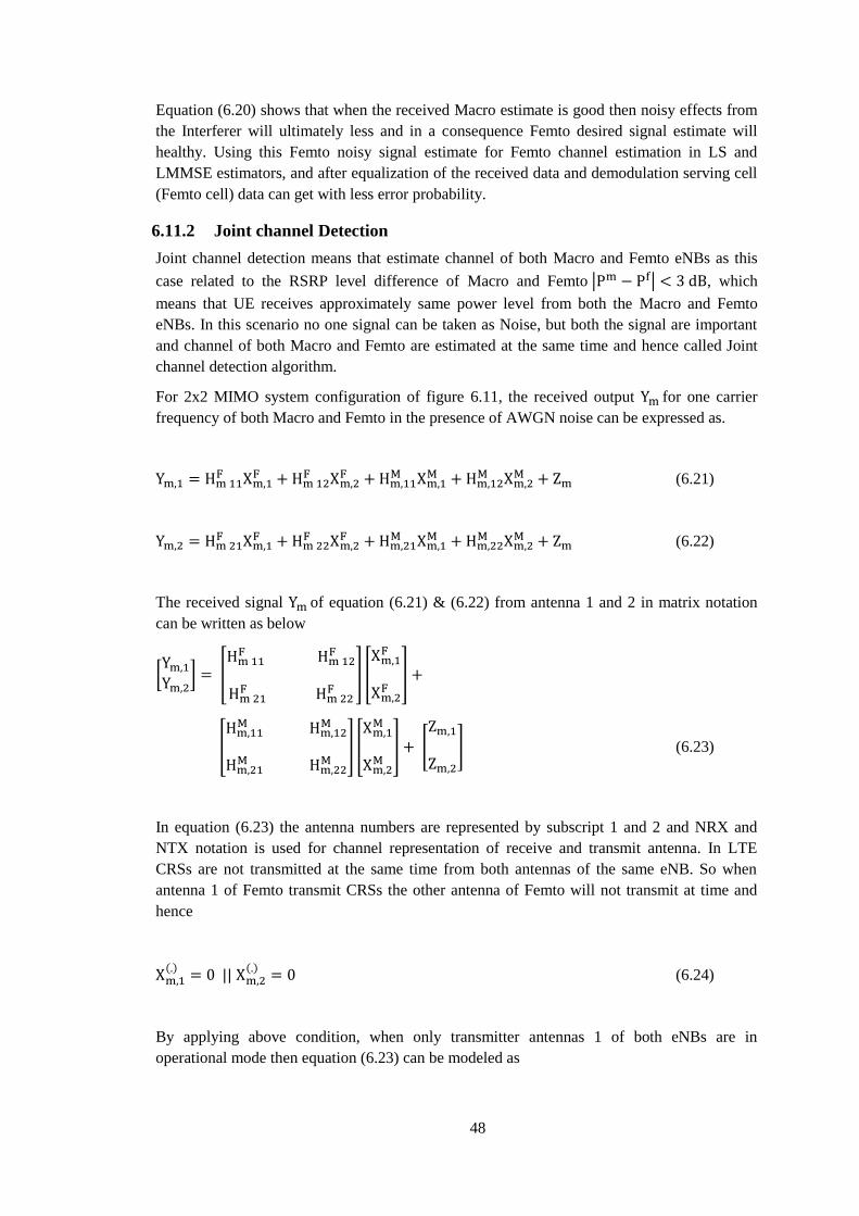
48

Equation (6.20) shows that when the received Macro estimate is good then noisy effects from

the Interferer will ultimately less and in a consequence Femto desired signal estimate will

healthy. Using this Femto noisy signal estimate for Femto channel estimation in LS and

LMMSE estimators, and after equalization of the received data and demodulation serving cell

(Femto cell) data can get with less error probability.

6.11.2 Joint channel Detection

Joint channel detection means that estimate channel of both Macro and Femto eNBs as this

case related to the RSRP level difference of Macro and Femto | | , which

means that UE receives approximately same power level from both the Macro and Femto

eNBs. In this scenario no one signal can be taken as Noise, but both the signal are important

and channel of both Macro and Femto are estimated at the same time and hence called Joint

channel detection algorithm.

For 2x2 MIMO system configuration of figure 6.11, the received output for one carrier

frequency of both Macro and Femto in the presence of AWGN noise can be expressed as.

(6.21)

(6.22)

The received signal of equation (6.21) & (6.22) from antenna 1 and 2 in matrix notation

can be written as below

[

] [

] [

]

[

] [

] [

] (6.23)

In equation (6.23) the antenna numbers are represented by subscript 1 and 2 and NRX and

NTX notation is used for channel representation of receive and transmit antenna. In LTE

CRSs are not transmitted at the same time from both antennas of the same eNB. So when

antenna 1 of Femto transmit CRSs the other antenna of Femto will not transmit at time and

hence

||

(6.24)

By applying above condition, when only transmitter antennas 1 of both eNBs are in

operational mode then equation (6.23) can be modeled as

49

[

] [

] [

] [

] (6.25)

In equation (6.25) there are four unknown i.e. two Femto channel impulse responses

(

) and two Macro channel impulse response (

). From above

equation it is not possible to determine the values of four unknown parameters while using

single CRS symbol. So in order to take the advantage of time invariant characteristics of the

channel, as in LTE with in a resource block (RB) channel remain constant as far as the

Doppler spread remains small. So,

(6.26)

While following the above condition, for 2x2 MIMO system configurations with in a RB

symbol 1 and symbol 4 have the CRS as shown in a figure 2.8 . The equation (6.25) can be

reformed as below;

[

] [

] [

] [

] (6.27)

By taking the pseudo inverse of

Matrix, channel impulse response of

,

can be calculated as:

[

] ([

] [

]) [

]

(6.28)

By using similar calculation, remain channel impulses responses of Femto

and

Macro

can be calculated as fallow:

[

] ([

] [

]) [

]

(6.29)

Using equation (6.28) and (6.29) Macro and Femto cell channel at CRS position are

calculated. The pseudo inverse in equation (6.28) and (6.29) is actually least square estimate

at CRS positions. LMMSE can be applied to the Joint detection LS estimate for better

accuracy and performance by removing unwanted noise as appears in LS estimate equations.

Equations (6.17) to (6.20) are used for the interference cancelation while using LS estimate of

50

Macro channel estimate in order to minimize the effect of Macro interference on Femto

signal.

6.11.3 No IC

In No IC case the Femto eNB power is greater than Macro eNB i.e. . In this

case either the UE is much closer to the HeNB or Macro eNB is too far away from HeNB and

the RSRP level difference is to enough that UE can correctly estimate the Femto channel and

demodulate the Femto received data with accuracy.

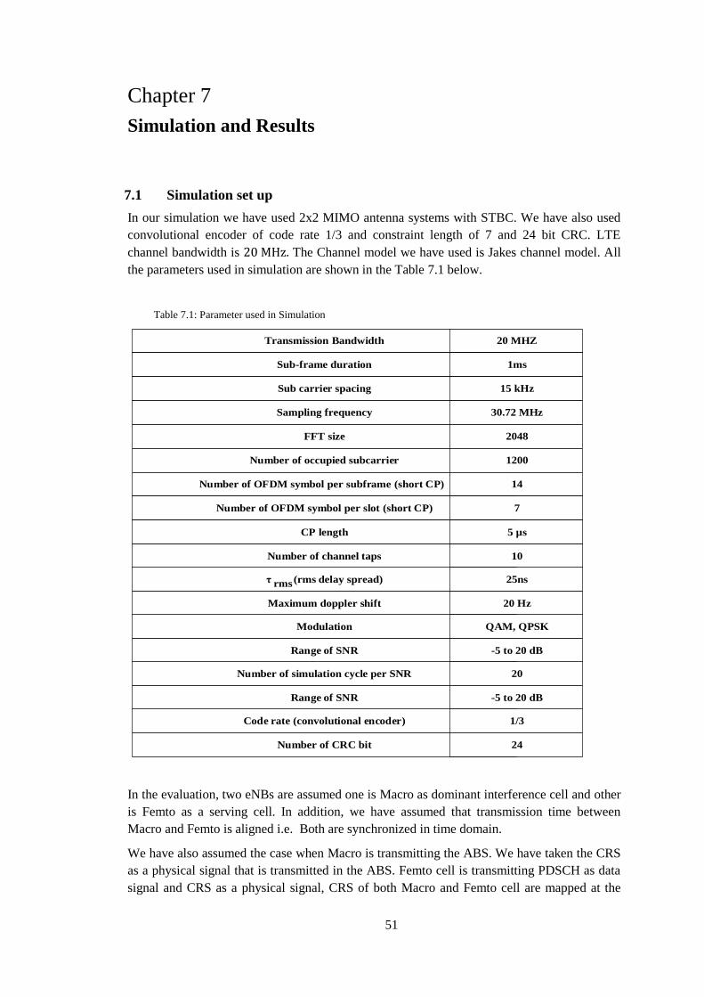
51

Chapter 7

Simulation and Results

Simulation set up 7.1

In our simulation we have used 2x2 MIMO antenna systems with STBC. We have also used

convolutional encoder of code rate 1/3 and constraint length of 7 and 24 bit CRC. LTE

channel bandwidth is The Channel model we have used is Jakes channel model. All

the parameters used in simulation are shown in the Table 7.1 below.

Table 7.1: Parameter used in Simulation

Transmission Bandwidth 20 MHZ

Sub-frame duration 1ms

Sub carrier spacing 15 kHz

Sampling frequency 30.72 MHz

FFT size 2048

Number of occupied subcarrier 1200

Number of OFDM symbol per subframe (short CP) 14

Number of OFDM symbol per slot (short CP) 7

CP length 5 µs

Number of channel taps 10

τ (rms delay spread) 25ns

Maximum doppler shift 20 Hz

rms

Modulation QAM, QPSK

Range of SNR -5 to 20 dB

Number of simulation cycle per SNR 20

Range of SNR -5 to 20 dB

Code rate (convolutional encoder) 1/3

Number of CRC bit 24

In the evaluation, two eNBs are assumed one is Macro as dominant interference cell and other

is Femto as a serving cell. In addition, we have assumed that transmission time between

Macro and Femto is aligned i.e. Both are synchronized in time domain.

We have also assumed the case when Macro is transmitting the ABS. We have taken the CRS

as a physical signal that is transmitted in the ABS. Femto cell is transmitting PDSCH as data

signal and CRS as a physical signal, CRS of both Macro and Femto cell are mapped at the

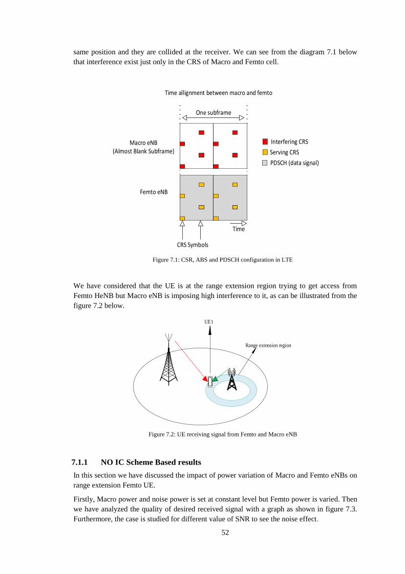
52

same position and they are collided at the receiver. We can see from the diagram 7.1 below

that interference exist just only in the CRS of Macro and Femto cell.

Macro eNB(Almost Blank Subframe)

Femto eNB

One subframe

Interfering CRS

Serving CRS

PDSCH (data signal)

Time allignment between macro and femto

Time

CRS Symbols

Figure 7.1: CSR, ABS and PDSCH configuration in LTE

We have considered that the UE is at the range extension region trying to get access from

Femto HeNB but Macro eNB is imposing high interference to it, as can be illustrated from the

figure 7.2 below.

Range extension region

UE1

Figure 7.2: UE receiving signal from Femto and Macro eNB

7.1.1 NO IC Scheme Based results

In this section we have discussed the impact of power variation of Macro and Femto eNBs on

range extension Femto UE.

Firstly, Macro power and noise power is set at constant level but Femto power is varied. Then

we have analyzed the quality of desired received signal with a graph as shown in figure 7.3.

Furthermore, the case is studied for different value of SNR to see the noise effect.

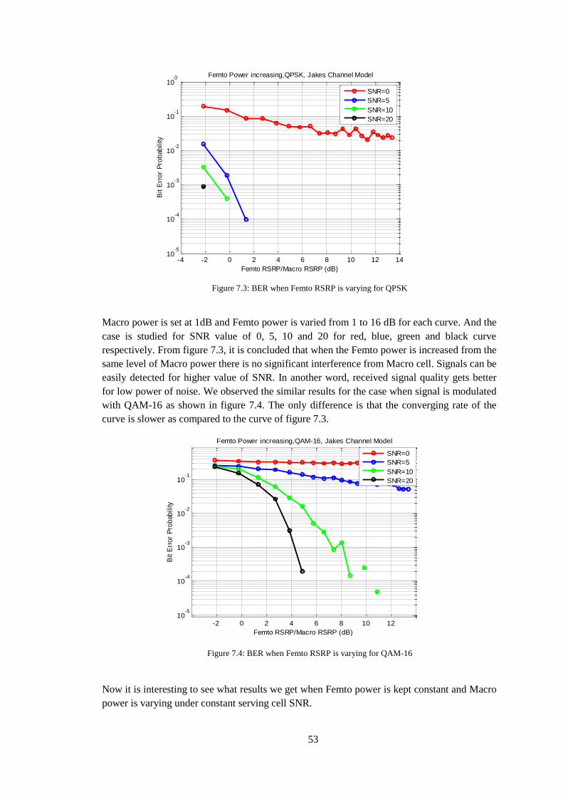
53

Figure 7.3: BER when Femto RSRP is varying for QPSK

Macro power is set at 1dB and Femto power is varied from 1 to 16 dB for each curve. And the

case is studied for SNR value of 0, 5, 10 and 20 for red, blue, green and black curve

respectively. From figure 7.3, it is concluded that when the Femto power is increased from the

same level of Macro power there is no significant interference from Macro cell. Signals can be

easily detected for higher value of SNR. In another word, received signal quality gets better

for low power of noise. We observed the similar results for the case when signal is modulated

with QAM-16 as shown in figure 7.4. The only difference is that the converging rate of the

curve is slower as compared to the curve of figure 7.3.

Figure 7.4: BER when Femto RSRP is varying for QAM-16

Now it is interesting to see what results we get when Femto power is kept constant and Macro

power is varying under constant serving cell SNR.

-4 -2 0 2 4 6 8 10 12 1410

-5

10-4

10-3

10-2

10-1

100 Femto Power increasing,QPSK, Jakes Channel Model

Femto RSRP/Macro RSRP (dB)

Bit E

rro

r P

rob

ab

ility

SNR=0

SNR=5

SNR=10

SNR=20

-2 0 2 4 6 8 10 1210

-5

10-4

10-3

10-2

10-1

Femto Power increasing,QAM-16, Jakes Channel Model

Femto RSRP/Macro RSRP (dB)

Bit E

rro

r P

rob

ab

ility

SNR=0

SNR=5

SNR=10

SNR=20

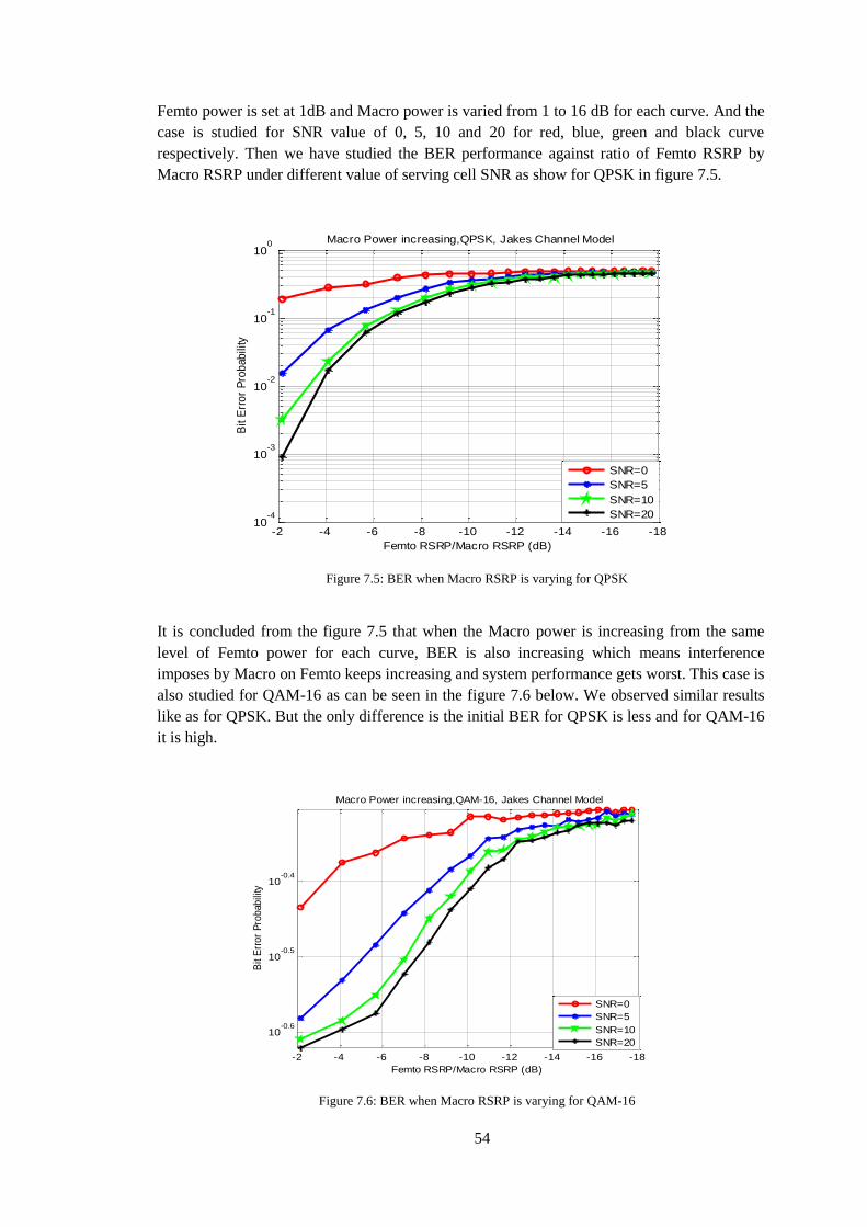
54

Femto power is set at 1dB and Macro power is varied from 1 to 16 dB for each curve. And the

case is studied for SNR value of 0, 5, 10 and 20 for red, blue, green and black curve

respectively. Then we have studied the BER performance against ratio of Femto RSRP by

Macro RSRP under different value of serving cell SNR as show for QPSK in figure 7.5.

Figure 7.5: BER when Macro RSRP is varying for QPSK

It is concluded from the figure 7.5 that when the Macro power is increasing from the same

level of Femto power for each curve, BER is also increasing which means interference

imposes by Macro on Femto keeps increasing and system performance gets worst. This case is

also studied for QAM-16 as can be seen in the figure 7.6 below. We observed similar results

like as for QPSK. But the only difference is the initial BER for QPSK is less and for QAM-16

it is high.

Figure 7.6: BER when Macro RSRP is varying for QAM-16

-18-16-14-12-10-8-6-4-210

-4

10-3

10-2

10-1

100 Macro Power increasing,QPSK, Jakes Channel Model

Femto RSRP/Macro RSRP (dB)

Bit

Err

or

Pro

bab

ility

SNR=0

SNR=5

SNR=10

SNR=20

-18-16-14-12-10-8-6-4-2

10-0.6

10-0.5

10-0.4

Macro Power increasing,QAM-16, Jakes Channel Model

Femto RSRP/Macro RSRP (dB)

Bit

Err

or

Pro

bab

ility

SNR=0

SNR=5

SNR=10

SNR=20

55

Finally, in No IC scheme Femto power and Macro power is kept constant at different RSRP

level and serving cell SNR is varying from -5dB to 20dB. Then we have studied the BER

performance against ratio of Femto RSRP by serving cell SNR and results for QPSK and

QAM are shown in figure 7.7 and figure 7.8.

Figure 7.7: BER when SNR is varying for QPSK

From the above figure 7.7 we examined that interference exist when the power level of Macro

RSRP is greater or equals to 3 dB with respect to Femto RSRP. This is due to the fact that

stronger the Macro power, channel estimation quality degrade more. As mentioned before

channel estimation in LTE is based upon CRS signals. And RSRP is the linear average power

of the received CRS. The nonlinear characteristics from SNR 3 dB to 6 dB in the blue or

curve with asterisk can be removed if we send more number of sub-frames; in this graph we

have transmitted just 20 sub-frames. We have transmitted 1500 sub-frames for block error rate

calculation and there are no such non-linearities as you can see the block error rate in figure

7.11 and 7.12.

In the case of QAM-16 the results are worst as QAM symbol have more bits per symbol and

results are shown in figure 7.8 below.

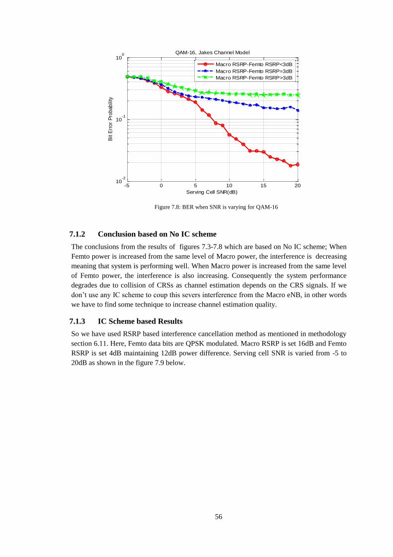
56

Figure 7.8: BER when SNR is varying for QAM-16

7.1.2 Conclusion based on No IC scheme

The conclusions from the results of figures 7.3-7.8 which are based on No IC scheme; When

Femto power is increased from the same level of Macro power, the interference is decreasing

meaning that system is performing well. When Macro power is increased from the same level

of Femto power, the interference is also increasing. Consequently the system performance

degrades due to collision of CRSs as channel estimation depends on the CRS signals. If we

don’t use any IC scheme to coup this severs interference from the Macro eNB, in other words

we have to find some technique to increase channel estimation quality.

7.1.3 IC Scheme based Results

So we have used RSRP based interference cancellation method as mentioned in methodology

section 6.11. Here, Femto data bits are QPSK modulated. Macro RSRP is set 16dB and Femto

RSRP is set 4dB maintaining 12dB power difference. Serving cell SNR is varied from -5 to

20dB as shown in the figure 7.9 below.

-5 0 5 10 15 2010

-2

10-1

100 QAM-16, Jakes Channel Model

Serving Cell SNR(dB)

Bit

Err

or

Pro

bab

ility

Macro RSRP-Femto RSRP<3dB

Macro RSRP-Femto RSRP=3dB

Macro RSRP-Femto RSRP>3dB

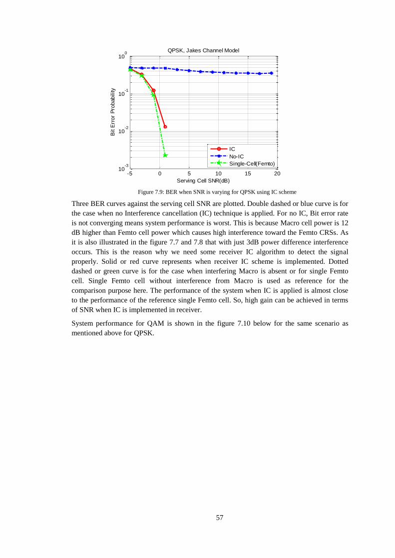
57

Figure 7.9: BER when SNR is varying for QPSK using IC scheme

Three BER curves against the serving cell SNR are plotted. Double dashed or blue curve is for

the case when no Interference cancellation (IC) technique is applied. For no IC, Bit error rate

is not converging means system performance is worst. This is because Macro cell power is 12

dB higher than Femto cell power which causes high interference toward the Femto CRSs. As

it is also illustrated in the figure 7.7 and 7.8 that with just 3dB power difference interference

occurs. This is the reason why we need some receiver IC algorithm to detect the signal

properly. Solid or red curve represents when receiver IC scheme is implemented. Dotted

dashed or green curve is for the case when interfering Macro is absent or for single Femto

cell. Single Femto cell without interference from Macro is used as reference for the

comparison purpose here. The performance of the system when IC is applied is almost close

to the performance of the reference single Femto cell. So, high gain can be achieved in terms

of SNR when IC is implemented in receiver.

System performance for QAM is shown in the figure 7.10 below for the same scenario as

mentioned above for QPSK.

-5 0 5 10 15 2010

-3

10-2

10-1

100

QPSK, Jakes Channel Model

Serving Cell SNR(dB)

Bit E

rro

r P

rob

ab

ility

IC

No-IC

Single-Cell(Femto)

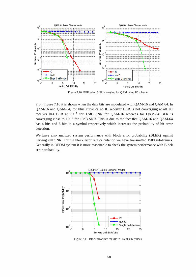
58

Figure 7.10: BER when SNR is varying for QAM using IC scheme

From figure 7.10 it is shown when the data bits are modulated with QAM-16 and QAM 64. In

QAM-16 and QAM-64, for blue curve or no IC receiver BER is not converging at all. IC

receiver has BER at for 13dB SNR for QAM-16 whereas for QAM-64 BER is

converging close to for 19dB SNR. This is due to the fact that QAM-16 and QAM-64

has 4 bits and 6 bits in a symbol respectively which increases the probability of bit error

detection.

We have also analyzed system performance with block error probability (BLER) against

Serving cell SNR. For the block error rate calculation we have transmitted 1500 sub-frames.

Generally in OFDM system it is more reasonable to check the system performance with Block

error probability.

Figure 7.11: Block error rate for QPSK, 1500 sub-frames

-5 0 5 10 15 20 2510

-3

10-2

10-1

100

IC,QPSK, Jakes Channel Model

Serving cell SNR(dB)

Blo

ck E

rror

Pro

ba

bilit

y

IC

NO IC

Single cell (femto)

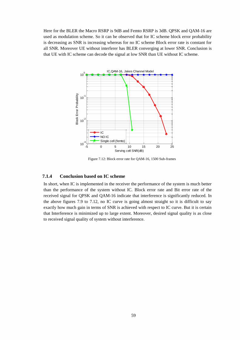
59

Here for the BLER the Macro RSRP is 9dB and Femto RSRP is 3dB. QPSK and QAM-16 are

used as modulation scheme. So it can be observed that for IC scheme block error probability

is decreasing as SNR is increasing whereas for no IC scheme Block error rate is constant for

all SNR. Moreover UE without interferer has BLER converging at lower SNR. Conclusion is

that UE with IC scheme can decode the signal at low SNR than UE without IC scheme.

Figure 7.12: Block error rate for QAM-16, 1500 Sub-frames

7.1.4 Conclusion based on IC scheme

In short, when IC is implemented in the receiver the performance of the system is much better

than the performance of the system without IC. Block error rate and Bit error rate of the

received signal for QPSK and QAM-16 indicate that interference is significantly reduced. In

the above figures 7.9 to 7.12, no IC curve is going almost straight so it is difficult to say

exactly how much gain in terms of SNR is achieved with respect to IC curve. But it is certain

that Interference is minimized up to large extent. Moreover, desired signal quality is as close

to received signal quality of system without interference.

-5 0 5 10 15 20 2510

-3

10-2

10-1

100

IC,QAM-16, Jakes Channel Model

Serving cell SNR(dB)

Blo

ck E

rror

Pro

ba

bilit

y

IC

NO IC

Single cell (femto)

60

Chapter 8

Conclusion and Future work

Conclusion 8.1

In this thesis, we have analyzed Femto cell UE in the Heterogeneous network of LTE, which

is in the cell extension region trying to get access from Femto cell. Since in LTE

heterogeneous network Macro and Femto cell operates with same set of frequencies therefore

there is always possibility of inter-cell interference especially when received signal power

from interfering cell is high. As we have mentioned in problem definition that with the usage

of ABS interference towards the data signal is eliminated however there is a chance that CRSs

collide and create interference. Creating this environment in the Matlab simulation we

implemented comIC algorithm to reduce the impact of colliding CRSs. If we see the IC

schemes based results in 7.1.3 graph shows that interference is minimized and brought it

down to acceptable range. Above all, quality of received signal is way better than the received

signal without IC algorithm.

As mentioned earlier cell ID and RSRP of both Macro and Femto cells are known to UE.

Based upon the investigation on Macro and Femto cell RSRP difference level and Matlab

simulation results proves that when the RSRP of Interfering cell is higher or equal to the

RSRP of serving cell Interference is detected, due to which Femto UE may not access Femto

cell at all. For the case when Macro RSRP is greater than Femto RSRP by 3dB, simulation

result shows that receiver with IC has system performance almost close to the system without

interference. However, for receiver with no IC, Bit error rate is not converging meaning that

system is not performing well.

Furthermore, quantity of noise in the system makes a huge difference in a quality of the

received signal. To see the effect of noise we have simulated the system without IC algorithm

under 5, 10, 15, 20 dB SNR values. We plot the graph of BER versus Femto RSRP/Macro

RSRP in dB. Here the Femto RSRP is desired signal power and Macro RSRP is interfering

signal power. The graph shows received signal quality gets better and better under 5, 10, 15,

20 dB SNR values respectively.

In LTE, PDSCH channel (data and multimedia) is modulated with QPSK, QAM-16 or QAM-

64 as high data rate is expected due to which we have also simulated with QPSK and 16

QAM. Received signal quality is better for QPSK than QAM-16 as QPSK has lower number

of states then QAM. For better detection of signal we have appended 24 bit CRC followed by

convolutional encoder. For a single system without interference convolutional encoder

provides around 7dB gain in terms of SNR, Which is shown in the figure 6.3. As interference

is the cause of power difference between two cells, to vary the signal power we have included

RAPP power amplifier model.

61

Future Work 8.2

We have studied the case when there is only one interfering eNB; it is interesting to

see for interfering cell more than one.

It would be clearer picture of the system if the result is compared with non-colliding

CRS case.

Here we have used LS and LMMSE for channel estimation, Implementation of IC

algorithm with different channel estimation technique can be interesting.

Interesting to see what will happen when two Femto UEs are in cell extension region.

62

References

[1] Beatriz Soret, Yuanye Wang, Klaus I. Pedersen, "CRS Interference Cancellation in

Heterogeneous Networks for LTE-Advanced Downlink," in International Workshop on

Small Cell Wireless Networks, 2012.

[2] Huang, W. X. Ming, "Macro-Femto Inter-Cell Interference Mitigation for 3GPP LTE-A

Downlink," pp. 75-80, 2012.

[3] 3GPP, R1-104036, "Investigation on CRS Interference Transmitted to Downlink control

Channel," NTT DOCOMO, july 2010.

[4] Lopes-Perez D; Chu Xiaoli, "Inter-Cell Interference Coordination for Expanded Region

Picocells in Heterogeneous Networks," pp. 1 - 6, 2011.

[5] Motorola Inc., "Long term evolution(LTE)," Technical white paper, p. 2, 2007.

[6] Ergen, Mustafa, Mobile Broadband Including WiMAX and LTE, Berkeley, CA: 2009.

[7] Telesystem Innovations Inc., "The Physical Layer WHITE PAPER," LTE in a Nutshell,

2010.

[8] Daniel Larsson, "Analysis of channel estimation methods for OFDMA," Master of

Science Thesis , Stockholm, Sweden, 2006-12-19.

[9] Prasad, R. van NeeR, OFDM for Wireless Multimedia Communications, London: Artech

publishers, January 2000.

[10] Erik Dahlman, Stefan Parkvall & Johan Skold, 4G: LTE/LTE-advanced, Academic Press,

2011.

[11] Anritsu Corporation, "LTE resource guide".

[12] Jim Zyren, Dr. Wes McCoy, Technical Editor, "Overview of the Long TermEvolution

Physical Layer," vol. Document Number: 3GPPEVOLUTIONWP, Rev 2007.

[13] "LTE, Evolved Universal Terrestrial Radio Access (E-UTRA),Physical channels and

modulation," vol. 3GPP TS 36.211 version 10.0.0 Release 10, Jan 2011.

[14] Hisham El Shear, "Interference Management in LTE-Advanced Heterogeneous Networks

Using Almost Blank Sub-frame," KTH, 2012.

[15] K. R. Wondmenech A.M, "''Load Balancing in Heterogenous LTE-A Networks'',"

Linkoping University, Sweden , Jun 2012.

[16] "Mobile data traffic surpasses voice," Ericsson, March 2010. [Online]. Available:

http://www.ericsson.com/news/1396928.

[17] Damnjanovic A., Wei, Yongbin, "A SURVEY ON 3GPP HETEROGENEOUS, Wireless

Communications," vol. 18, no. 3, June 2011.

63

[18] LTE,3GPP TS 36.211, " Evolved Universal Terrestrial Radio Access (E-UTRA);

Physical channels and modulation," vol. version 10.0.0 Release 10, 2010.

[19] 3GPP, RP-080671, "Modification to the RSRP definition," in Nokia, Nokia Siemens,

Warsaw, Poland, July 4, 2008.

[20] 3GPP, RP-100205, "Modification of RSRQ definition," in NTT DOCOMO, Valencia,

Spain, January 18 – 22, 2010.

[21] "3GPP, Evolved Universal Terrestrial Radio Access (E-UTRA); User Equipment (UE)

procedures in idle mode," vol. 8.0.0, p. Tech. Spech. 36.304, December 2007.

[22] 3GPP, R1-100701, "Importance of serving cell selection in heterogeneous networks," in

Qualcomm Inc, Jan 2010.

[23] 3GPP, "EUTRA and EUTRAN overall description," Stage 2, TS 36.300, vol. 8.10.0.

[24] Clercks, Claude Oestges and B., "MIMO Wireless Communications:From Real-World

Propagation to Space-Time Code Design," Elsevier, 2007.

[25] Asad Mehmood, Waqas Aslam Cheema, "Channel Estimation for LTE Downlink,"

Blekinge Institute of Technology, Master Thesis Report, Sweden, September 2009.

[26] Rappaport T., Wireless Communications, principles and Practice, NJ, USA: Prentice-

Hall, Englewood Cliffs, 1996.

[27] Goldsmith, Andrea, Wireless Communication, 2005.

[28] Irshad, Yasir, On Some continuous-time modeling and estimation problems for control,

Karlstad, Sweden: Karlstad University, 2013.

[29] Jakes, W.C., Microwave Mobile Communications, New York: Wiley, 1974.

[30] Ove Edfors, Magnus Sandell, Jan-Jaap van de Beek, Sarah Kate Wilson and Per Ola

Börjesson, "OFDM Channel Estimation by Singular Value Decomposition," IEEE

TRANSACTION ON COMMUNICATIONS, Vols. 46, NO 7, July 1998.

[31] Ye (Geoffrey) Li, Leonard J. Cimini and Nelson R. Sollenberger, "Robust Channel

Estimation for OFDM Systems with Rapid Dispersive Fading Channels," IEEE

TRANSACTION ON COMMUNICATIONS, Vols. 46, NO 7, July 1998.

[32] Jan-Jaap van Beek; Ove Edfors; Magnus Sandell; Sarah Kate Wilson; Per Ola Börjesson,

"On Channel Estimation in OFDM Systems," In proceedings of Vehicular Technology

Conference (VTC’95), vol. 2, pp. 815-819, September 1995.

[33] al, Jose Araujo et, "Self Triggered Control over Wireless Sensor and Actuator

Networks," KTH Royal Insitute of Technology, Technical report, Stockholm.

[34] Regmi, Raju, "Effects of Quantization Noise in Telecommunication Systems," Karlstad

University , Karlstad, Sweden, 2012-10-12.

64

[35] P. Mu˜noz, I. de la Bandera, R. Barco, F. Ruiz, M. Toril and S. Luna-Ram´ırez,

"Estimation of link-layer Quality parameter in system level LTE link simulators,"

University of M' alaga, Communication dept., Spain.

[36] Ho-Chul Jung, Chang-Ju Kim, Hyung-Rae Park and Jong-Ho Kim, "A comparative

performance analysis of STBC-OFDM system under Rayleigh fading environments,"

School of Avionics and Telecommunications Engineering, Hankuk Aviation University.

[37] Peterson, W. W. and Brown, D.T, "Cyclic Codes for Error Detection.," In Proceedings of

the IRE, p. 228–235, January 1961.

[38] Costello, S. Lin and D. J., Error Control Coding, Englewood Cliffs, NJ: Prentice Hall,

1982.

[39] Gokceoglu, Ahmet Hasim, "Performance of Adaptive feed forward methods in wideband

power amplifier linearization," Tampere University of Technology, Oct 2009.

65

Appendix A

A.1 LTE resource grid for LTE minimum bandwidth (1.4 MHz)

Figure A.1: LTE Resource grid for 1.4MHz bandwidth

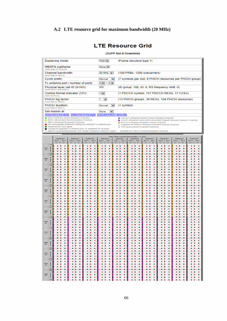
66

A.2 LTE resource grid for maximum bandwidth (20 MHz)

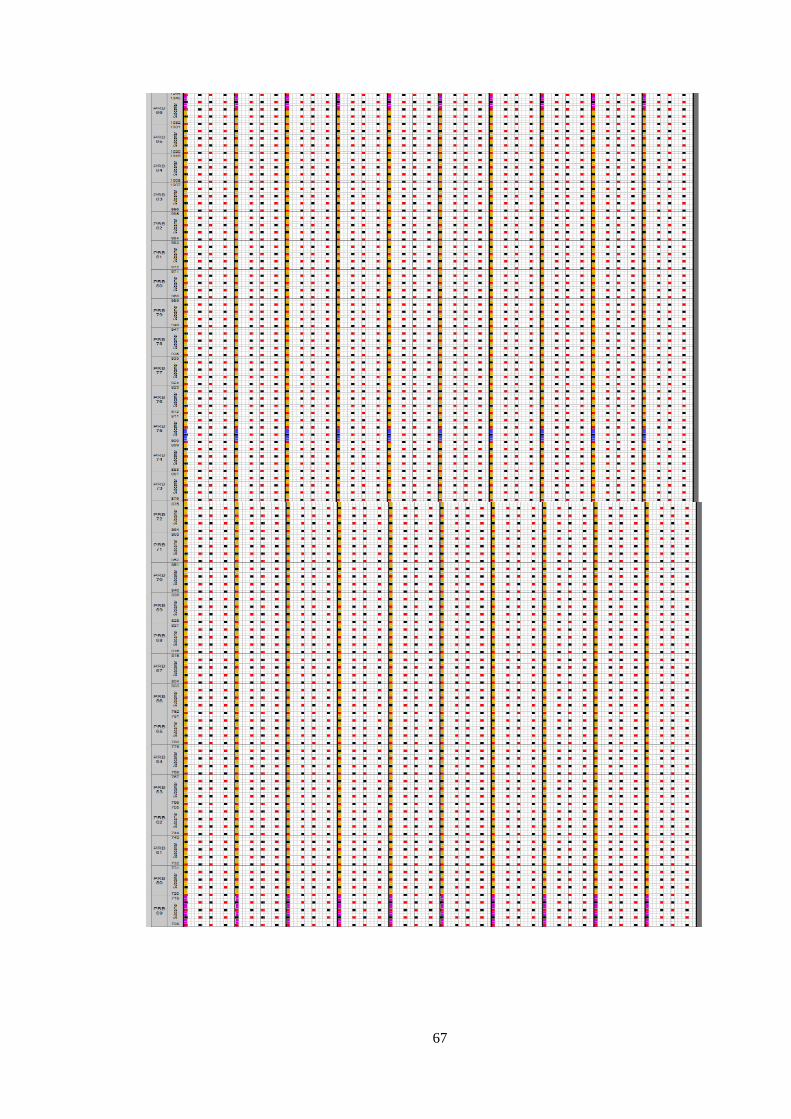
67

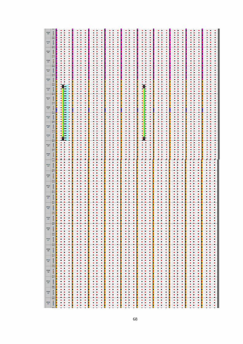
68

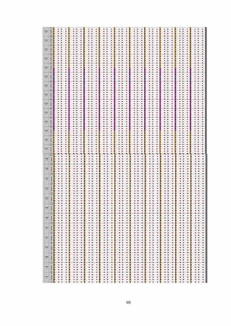
69

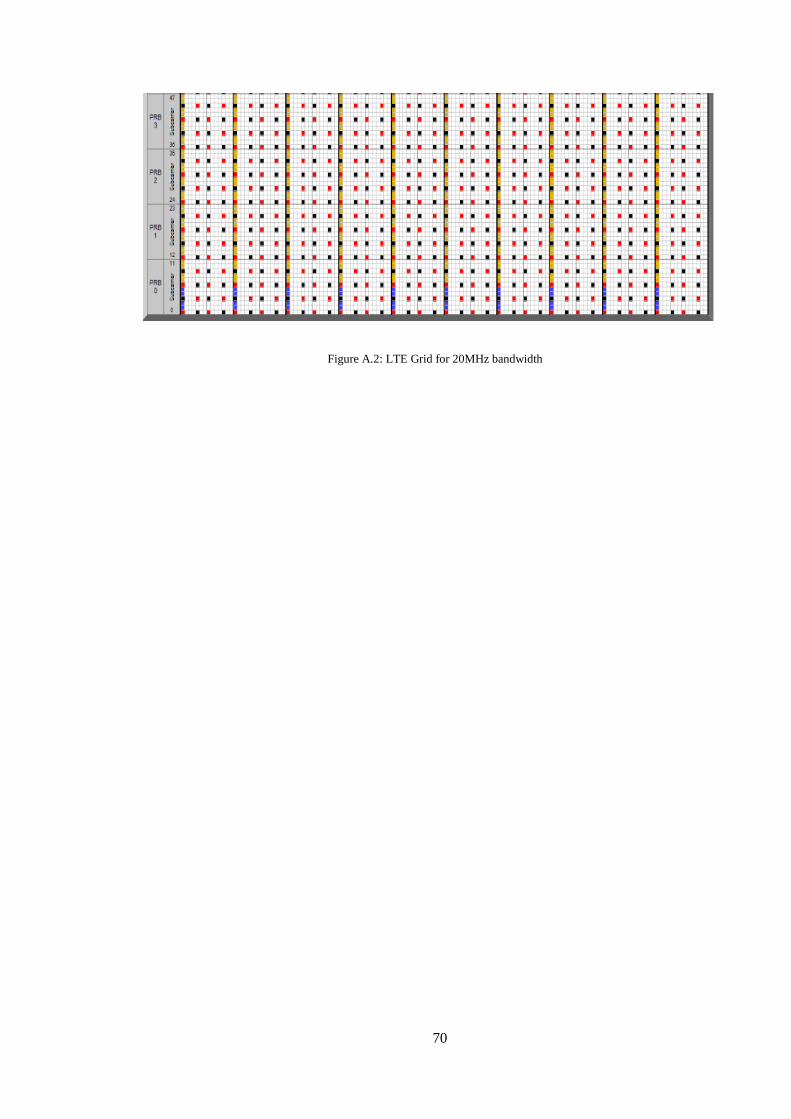
70

Figure A.2: LTE Grid for 20MHz bandwidth