Embed Size (px)
Citation preview

General rights Copyright and moral rights for the publications made accessible in the public portal are retained by the authors and/or other copyright owners and it is a condition of accessing publications that users recognise and abide by the legal requirements associated with these rights.
• Users may download and print one copy of any publication from the public portal for the purpose of private study or research. • You may not further distribute the material or use it for any profit-making activity or commercial gain • You may freely distribute the URL identifying the publication in the public portal
If you believe that this document breaches copyright please contact us providing details, and we will remove access to the work immediately and investigate your claim.
Downloaded from orbit.dtu.dk on: May 19, 2018
Understanding and simulating vibrations of plain bridge cables under varyingmeteorological conditionsWind tunnel experimental work and analytical modelling
Matteoni, Giulia; Georgakis, Christos T.; Ricciardelli, Francesco; Arentoft, Mogens; Koss, Holger;Svensson, Eilif
Publication date:2014
Document VersionPeer reviewed version
Link back to DTU Orbit
Citation (APA):Matteoni, G., Georgakis, C. T., Ricciardelli, F., Arentoft, M., Koss, H., & Svensson, E. (2014). Understanding andsimulating vibrations of plain bridge cables under varying meteorological conditions: Wind tunnel experimentalwork and analytical modelling. DTU Tryk.

Understanding and simulating vi-brations of plain bridge cablesunder varying meteorological con-ditions
- Wind tunnel experimental work and analytical mod-elling
G. Matteoni
Ph.D. Thesis
Department of Civil EngineeringTechnical University of Denmark
2013
Supervisors:
Associate Professor C.T. Georgakis, DTU BygAssociate Professor H.H. Koss, DTU BygAssociate Professor F. Ricciardelli, University of Reggio CalabriaMogens Arentoft, IPUEilif Svensson, ES-Consult A/S
Assesment Committee:
Professor Jasna B. Jakobsen, University of StavangerDoctor John Macdonald, University of BristolAssociate Professor Gregor Fischer, DTU Byg
Understanding and simulating vibrations of plain bridge cablesunder varying meteorological conditions-Wind tunnel experimental work and analytical modelling
Copyright c© 2013 by G. MatteoniPrinted by DTU-TrykDepartment of Civil EngineeringTechnical University of DenmarkISBN: 1234567891234ISSN: 1234-5678

a Tommaso, con affetto

Preface
This thesis is submitted in partial fulfilment of the requirements for theDanish Ph.D. degree. The work has been carried out at the Department ofCivil Engineering at the Technical University of Denmark in collaborationwith IPU and took place in the period between May 2010 to July 2013, withAssociate Professor Christos T. Georgakis as main supervisor and AssociateProfessor Holger Koss, Associate Professor Francesco Ricciardelli, MogensArentoft and Eiliff Svensson as co-supervisors.
This thesis is based upon published and under-review articles in ISI jour-nals. The first chapter gives a literature review on bridge cable vibrationphenomena under varying meteorological conditions, while each of the sub-sequent four chapters are made up by separate and unedited reproduction ofabove mentioned journal papers. Lastly, the combined work is discussed andconclusions are made in respect to the initially introduced problems, togetherwith other outcomes of the work.
Kongens Lyngby, the 31st July 2013
G. Matteoni
Preface to published version
The thesis was defended at a public defence on the ... . The official assess-ment committee consisted of Associate Professor Gregor Fischer (chairman),Technical University of Denmark, Doctor John Macdonald, University ofBristol, and Professor Jasna B. Jakobsen, University of Stavanger.
iv

Kongens Lyngby, the 31st July 2013
G. Matteoni


Acknowledgements
My first debt of gratitude goes to my supervisor, Associate Professor ChristosT. Georgakis, who has patiently provided the vision, encouragement andadvise necessary to complete the project, while leaving at the same timegreat freedom to pursue independent work.
Special thanks go to all my co-supervisors, Associate Professor HolgerKoss, Associate Professor Francesco Ricciardelli, Mogens Arentoft and EilifSvensson, for their support, guidance and helpful suggestions.
I acknowledge the financial support from Femern Belt A/S, funding theconstruction of a state of the art wind tunnel testing facility, which made allthis possible.
I’d like to express my gratitude to the technicians at DTU-BYG, in par-ticular Keld Plougmann, Robert Svan and Erik Bjørn Kristiansen, for theirpatience and precious work.
A special thank goes to the PhD student Cristoforo Demartino, whocollaborated to the analytical model.
Thanks to all other fellow students and PhDs for direct help or inspiration,in particular Nina Gall Jørgensen, Joan Hee Roldsgaard, Mia Schou MøllerLund, Anna Emilie Thybo, Annett Anders, Ieva Paegle, Antonio Acampora,Jan Winkler, Kenneth Kleissl, Emanuele Mattiello, Mads Beedholm Eriksen,Rocco Custer, Shouyung Zhan.
Thanks to my family, who always encouraged me during this very longstay in Denmark, to my friends, and to Rocco for his loving support.
vii


Abstract
The dissertation investigates the phenomenon of wind induced vibration ofbridge cables under varying meteorological conditions. A twin research ap-proach is adopted, where wind tunnel investigation of full-scale bridge cablesection models is paralleled with theoretical modelling.
A literature review on bridge cable vibration mechanisms under the threesurface states possibly achieved by cables, i.e. dry, wet and iced, was firstundertaken. The study helped to systematize the understanding of the ex-citation phenomena occurring in the different climatic conditions, based onresults of full-scale monitoring, wind tunnel testing and theoretical modelling.
An extensive wind tunnel test campaign was then undertaken in orderto further understand the onset conditions and characteristics of instabilityin the different climatic conditions described in the literature. Tests wereseparated into two different categories, i.e. static and passive-dynamic.
Static wind tunnel tests were performed in dry surface conditions, forvarying Reynolds number, turbulence intensity, cable-wind angle, and angle-of-attack. It was understood that dry instability is very sensitive to micro-scopic imperfections of the cable surface, such as deviations from the nomi-nal shape of the external HDPE tubing or alterations of its inherent surfaceroughness. It was in fact observed that in the critical Reynolds number range,while the drag coefficient is consistent with changes in the angle-of-attack,the lift coefficient exhibits marked variations. This variation is sufficient togenerate negative quasi-steady aerodynamic damping, and thus to potentialylead to galloping instability.
Passive dynamic wind tunnel tests were subsequently undertaken for acable section model of the same type as the one tested in static conditions.Tests were undertaken at a critical cable-wind angle for the occurrence ofdry inclined galloping, for varying Reynolds numbers and angles-of-attack.As confirmation of the findings from the static tests, it was observed thatthe dynamic response of the cable section, i.e. in terms of peak-to-peakamplitudes and aerodynamic damping, changes consistently with Reynoldsnumber, for the tested wind angles-of-attack. In fact, for selected angles-of-
ix

attack, the response was stable thoughout the whole tested range of Reynoldsnumber, while for other angles, negative aerodynamic damping, accompaniedby large amplitude peak to peak amplitudes, occurred. This latter behaviourwas likely to be associated to dry inclined galloping.
Passive dynamic wind tunnel tests were finally undertaken in presenceof rain, using the same cable model as adopted in the dry state. The testsserved to improve the current understanding of the phenomenon of rain-wind induced vibration. Test results showed that when the a critical surfacetension is achieved for the cable sheating, an oscillating lower and upperwater rivulet form on its surface. The angular oscillation of the rivuletscontribute to amplify the vertical vibration of the cable, which becomes largein amplitude and is accompanied by negative aerodynamic damping. On theother hand, when the surface tension of the cable is too low a steady upperand lower non-coherent water rivulets form. These are not sufficient for theexcitation to get started, independently of the cable mass. The cable modelwas in fact manifestly stable and exhibited positive aerodynamic dampingthroughout the whole range of tested Reynolds number, being accompaniedby limited peak-to-peak amplitude.
A generalized quasi-steady 3 DOF analytical model for the prediction ofthe aerodynamic instability of a slender prism with generic cross section, i.e.either bluff or streamlined, immersed in unsteady wind flow, and character-ized by a general spatial orientation with respect to the wind direction, wasfinally developed. The model accounted for variation of the force coefficients,i.e. drag, lift, and moment, with Reynolds number based on the relative flowvelocity, with relative angle-of-attack, and relative cable-wind angle. Theaerodynamic forces acting on the structure were linearized about zero struc-tural velocities, structural rotation and about the steady component of thetotal wind velocity. Based on the analytical solution of the eigenvalue prob-lem, by applying the Routh-Hurwitz criterion, an expression of the minimumstructural damping and structural stiffness required to prevent aerodynamicinstabilities of galloping- and static divergence-type respectively are given.

Resume
Denne afhandling undersøger fænomenet vind-inducerede vibrationer af bro-kabler under forskellige meteorologiske forhold. Forskningsmetoden, der eranvendt, paralleliserer vindtunneltests udført pa sektioner af fuldskala bro-kabler med teoretisk modellering.
Det indledende litteraturstudium, der omhandlede vibrationsmekanismerfor brokabler under tre mulige overfladetilstande, tør, vad og iset, hjalp medat systematisere forstaelsen for de fænomener, der igang-sætter kabelvibra-tioner under forskellige klimatiske forhold. Studiet var baseret pa resultaterfra fuldskala overvagning, vindtunneltests og teoretisk modellering.
Et omfattende program for vindtunneltests blev igangsat for at opna endybere forstaelse for begyndel-sesbetingelserne og kendetegnene ved instabi-litet for de forskellige klimatiske forhold beskrevet i litteraturen.
Først blev statiske vindtunneltests udført pa sektioner af fuldskala bro-kabler orienteret vinkelret og skrat i forhold til vindretningen under tørre for-hold. Forsøgene blev udført for varierende Reynolds tal, angrebsvinkler samtturbulensintensiteter. De enkelte parametres betydning blev detaljeret evalu-eret. Det fremgik af forsøgene, at instabilitet af tørre kabler er yderst følsomover for mikroskopiske imperfektioner sasom afvigelser i den nominelle dia-meter af det ydre HDPE rør og forandringer i rørets naturlige overfladeruhed.Mens drag koefficienterne er konstante med ændringer i angrebsvinklen, udvi-ser lift koefficienterne en markant variation. Denne variation er tilstrækkeligtil at danne negativ kvasi-permanent aerodynamisk dæmpning og dermed te-oretisk set potentielt tilstrækkelig til at medføre galloping instabilitet. Passivedynamiske vindtunneltests blev efterfølgende foretaget pa samme kabeltypesom den, der var anvendt under de statiske forsøg. Forsøge blev udført for enkritisk kabel-vindvinkel med hensyn til dry inclined galloping. Denne kabel-vindvinkel var ligeledes blevet testet under statiske forhold.
De dynamiske forsøg blev udført for varierende Reynolds tal og angrebs-vinkler. Det blev observeret, at kabelsektionens dynamiske respons med hen-syn til peak-to-peak amplituder og aerodynamisk dæmpning ændres konsi-stent med Reynolds tallet for de undersøgte angrebsvinkler, hvilket bekræf-
xi

ter resultaterne fra de statiske tests. Responset var stabilt gennem hele dettestede interval af Reynolds tal for visse angrebsvinkler, hvorimod negativaerodynamisk dæmpning ledsaget af store peak-to-peak amplituder forekomfor andre angrebsvinkler. Sidstnævnte observation kan sandsynligvis associe-res med dry inclined galloping. Endvidere blev der udført passive dynamiskevindtunneltests under regnpavirkning ved at anvende den samme kabelmo-del, som var anvendt i tør tilstand. Disse forsøg tjente det formal at fa enforstaelse for to parametres betydning − kablets overfladespænding og mas-se − hvis indflydelse i tidligere forsøg ikke var blevet undersøgt detaljeret.Forsøgresultaterne viste, at nar overfladespændingen af kablet er for lav, vilder dannes en jævn øvre og nedre usammenhængende formation af løbenderegnvand. Disse er, uafhængigt af kablets masse, ikke tilstrækkelige til atinitiere instabilitet. Kablet var helt tydeligt stabilt og oplevede positiv aero-dynamisk dæmpning gennem hele det testede interval af Reynolds tal. Dettevar desuden ledsaget af begrænset peak-to-peak amplitude. Nar det rette ni-veau i overfladespænding derimod opnas, vil der forekomme en øvre og nedreoscillerende formation af løbende regn, hvilket udløser vibrationer med storamplitude. Disse vibrationer er ledsaget af negativ aerodynamisk dæmpningi et begrænset interval af Reynolds tal.
Endelig er en generel kvasi-permanent analytisk model med tre frihedsgra-der blevet udviklet. Modellen er i stand til at forudsige aerodynamisk insta-bilitet af et legeme med generelt tværsnit, dvs. enten bluff eller strømlinet,nedsænket i ikke-stationær vindstrømning og karakteriseret ved en generelrumlig orientering med hensyn til vindretningen. Modellen tager hensyn tilvariation i kraftkoefficienterne, dvs. drag, lift og moment, med et Reynolds talbaseret pa den relative vindhastighed, med relative angrebsvinkler og relativekabel-vindvinkler. De aerodynamiske kræfter, der virker pa konstruktionen,er lineariseret omkring nul strukturel hastighed, nul strukturel rotation ogomkring den steady komponent af den totale vindhastighed. Ved anvendelseaf Routh-Hurwitz kriteriet er en analytisk løsning pa egenværdiproblemet gi-vet, hvorved der er fundet et udtryk for den mindste strukturelle dæmpningog strukturelle stivhed pakrævet for at forhindre aerodynamisk galloping in-stabilitet og static divergence instabilitet.

Contents
1 Introduction 11.1 The research problem and the methodology . . . . . . . . . . 31.2 Thesis outline . . . . . . . . . . . . . . . . . . . . . . . . . . . 5
2 Background review 92.1 Introduction . . . . . . . . . . . . . . . . . . . . . . . . . . . . 102.2 Bridge cable aerodynamics . . . . . . . . . . . . . . . . . . . . 12
2.2.1 The quasi-steady assumption . . . . . . . . . . . . . . 142.2.2 Wind loading and force components . . . . . . . . . . . 152.2.3 Equations of motion . . . . . . . . . . . . . . . . . . . 222.2.4 Theoretical modelling . . . . . . . . . . . . . . . . . . . 23
2.3 Rain-wind induced vibration . . . . . . . . . . . . . . . . . . . 242.3.1 Field Measurements . . . . . . . . . . . . . . . . . . . 252.3.2 Dynamic wind tunnel tests . . . . . . . . . . . . . . . . 292.3.3 Static wind tunnel tests . . . . . . . . . . . . . . . . . 32
2.4 Dry state . . . . . . . . . . . . . . . . . . . . . . . . . . . . . 372.4.1 Field observations . . . . . . . . . . . . . . . . . . . . . 372.4.2 Dynamic wind tunnel tests . . . . . . . . . . . . . . . . 392.4.3 Static wind tunnel tests . . . . . . . . . . . . . . . . . 44
2.5 Iced state . . . . . . . . . . . . . . . . . . . . . . . . . . . . . 482.5.1 Field observations . . . . . . . . . . . . . . . . . . . . . 482.5.2 Dynamic wind tunnel tests . . . . . . . . . . . . . . . . 492.5.3 Static wind tunnel tests . . . . . . . . . . . . . . . . . 51
2.6 Conclusion . . . . . . . . . . . . . . . . . . . . . . . . . . . . . 52
3 Static wind tunnel tests 633.1 Introduction . . . . . . . . . . . . . . . . . . . . . . . . . . . . 633.2 Materials and Methods . . . . . . . . . . . . . . . . . . . . . . 66
3.2.1 Surface roughness and shape distortion measurements . 663.2.2 Wind tunnel tests . . . . . . . . . . . . . . . . . . . . . 67
3.3 Results and Discussion . . . . . . . . . . . . . . . . . . . . . . 70
xiii

3.3.1 Surface roughness and shape distortion measurements . 70
3.3.2 Wind tunnel tests . . . . . . . . . . . . . . . . . . . . . 73
3.4 Conclusion . . . . . . . . . . . . . . . . . . . . . . . . . . . . . 83
4 Passive-dynamic wind tunnel tests in dry state 87
4.1 Introduction . . . . . . . . . . . . . . . . . . . . . . . . . . . . 88
4.1.1 Overview of the dry inclined cable instability . . . . . . 88
4.1.2 Objectives and findings of the present investigation . . 90
4.2 Materials and Methods . . . . . . . . . . . . . . . . . . . . . . 91
4.2.1 Passive-dynamic wind tunnel tests . . . . . . . . . . . 91
4.2.2 Static wind tunnel tests . . . . . . . . . . . . . . . . . 96
4.3 Results and Discussion . . . . . . . . . . . . . . . . . . . . . . 98
4.3.1 Passive-dynamic wind tunnel tests . . . . . . . . . . . 98
4.3.2 Static wind tunnel tests . . . . . . . . . . . . . . . . . 103
4.4 Conclusion . . . . . . . . . . . . . . . . . . . . . . . . . . . . . 107
5 Passive-dynamic wind tunnel tests in wet state 113
5.1 Introduction . . . . . . . . . . . . . . . . . . . . . . . . . . . . 113
5.1.1 Interpretation of the excitation mechanism ofRWIV . . . . . . . . . . . . . . . . . . . . . . . . . . . 114
5.1.2 Objectives and results . . . . . . . . . . . . . . . . . . 116
5.2 Materials and Methods . . . . . . . . . . . . . . . . . . . . . . 117
5.2.1 Surface treatment . . . . . . . . . . . . . . . . . . . . . 117
5.2.2 Passive-dynamic wind tunnel tests . . . . . . . . . . . 118
5.3 Results and Discussion . . . . . . . . . . . . . . . . . . . . . . 124
5.3.1 Dry state . . . . . . . . . . . . . . . . . . . . . . . . . 124
5.3.2 Wet state . . . . . . . . . . . . . . . . . . . . . . . . . 124
5.4 Conclusion . . . . . . . . . . . . . . . . . . . . . . . . . . . . . 133
6 Analytical model 141
6.1 Introduction . . . . . . . . . . . . . . . . . . . . . . . . . . . . 142
6.2 Linearization of the aerodynamic and mechanical model . . . . 147
6.2.1 Flow around fixed inclined prism . . . . . . . . . . . . 147
6.2.2 Flow around moving inclined prism . . . . . . . . . . . 149
6.2.3 Aerodynamic forces . . . . . . . . . . . . . . . . . . . . 152
6.2.4 Structural properties and EOM . . . . . . . . . . . . . 154
6.3 State space representation . . . . . . . . . . . . . . . . . . . . 155
6.4 Eigenvalue problem and instability analysis . . . . . . . . . . . 158
6.5 Application of the 3 DOF model . . . . . . . . . . . . . . . . . 160
6.6 Conclusion . . . . . . . . . . . . . . . . . . . . . . . . . . . . . 164

7 Conclusions 1717.0.1 Future work . . . . . . . . . . . . . . . . . . . . . . . . 173
A Analytical model 177A.1 Derivation of the aerodynamic forces . . . . . . . . . . . . . . 177A.2 Flow variables linearization . . . . . . . . . . . . . . . . . . . 179A.3 Aerodynamic forces linearization . . . . . . . . . . . . . . . . 181A.4 Equations of motion . . . . . . . . . . . . . . . . . . . . . . . 186A.5 Terms of the characteristic polynomium . . . . . . . . . . . . . 188


Chapter 1
Introduction
The development of cable-stayed bridges as a structural choice for mediumto long span bridges has been remarkable through the closing decades of thelast century. Stay cables play an essential role in the dynamic behaviour ofcable-stayed bridges, and, being characterised by low mechanical damping,they are extremely vulnearable to wind excitation, (Fujino et al., 2012).
In the past years, numerous efforts have been made in order to understandthe mechanisms of various types of wind-induced cable vibration phenomenaand to find solutions for alleviating vibration problems. Some of the iden-tified mechanisms, particularly when related to inclined bridge cables, suchas rain-wind induced vibration, ice-induced vibrations, vortex-induced vi-bration at high reduced velocity and dry inclined galloping, generate seriouspreoccupation for the bridge designers. In fact, the associated vibration am-plitudes are much larger than for classical vibration mechanisms, for examplevortex-induced vibration or buffeting. Moreover, the excitation mechanismsof inclined cables still remain partially not understood, so that the amountof mechanical damping/stiffness necessary to couteract the vibration is stillunder discussion.
Rain-wind induced vibration represents the most frequently observed vi-bration mechanism on bridges. It was first recognised in 1988 at the Meiko-Nishi Bridge in Japan, during its period of construction. Here, the cablesexperienced large amplitude vibrations under the combination of certain windconditions, i.e. in terms of velocity and direction, only when it was raining,(Hikami and Shairaishi, 1988). Fig. 1.1 shows the first prototype observa-tion of rain water rivulet on the surface of a bridge cable, at the Meiko-NishiBridge, (Hikami and Shairaishi, 1988). After its first report, it became clearthat some other cable vibration episodes observed earlier for other bridges,could have been classified in the same category as rain-wind induced vibra-tion.
1

Introduction
Figure 1.1: Prototype observation of rain water rivulet along the lower sur-face of the cable at the Meiko-Nishi Bridge in Japan, (Hikami and Shairaishi,1988).
The excitation mechanisms of rain-wind induced vibration has been madeclearer in recent years, and some effective control methods have been suc-cessfully applied in practice.
Vortex-induced vibration at high reduced velocity and dry inclined gallop-ing are on the other hand less understood and would require more intensiveresearch attention. The dry inclined galloping, in particular, causes a verystrong concern since it has been suggested that it can result in undesiderablylarge amplitude motion. For example vibrations amplitudes of 1.5 m havebeen reported for the inclined cables of a cable-stayed a bridge in Japan,in dry conditions, under the occurrence of a typhoon, at wind velocity of18 m/s. The mechanism of excitation of such vibration episode has beeninterpreted as dry inclined galloping, (Matsumoto et al., 2010). Neverthe-less, bridge failures due to dry cable vibration have been reported to occurfor much lower wind velocities. For example, on February 2012, a vibrationaccident occurred at the Martin Olav Sabo Pedestrian Bridge in Minnesota,where the diaphragm plate holiding the cables to the main pylon fractured,see Fig. 1.2. The fracture was attributed to vibration of the cables occurringat low wind velocity, i.e. in the range of 2-5 m/s.
Numerous accidents have been reported for bridges worldwide in pres-ence of ice accretions on the cable surface. Such accretions can provoke thephenomenon of ice shedding, which consists in the falling of large pieces ofice/snow from the cable surface to the bridge deck, thus threatening the safetyof passengers. Moreover an aerodynamic modification of cable’s surface usu-ally occurs due to the ice formation which can lead to dynamic instabilitiesof galloping-type. Fig. 1.3 shows a view of the Toledo Skyway Bridge ca-bles in Ohio, which in 2011 experienced the formation of thick and heavy iceaccretions, leading to the bridge closure for several hours.
Episodes of inclined cable vibrations in the different meteorological con-
2 Department of Civil Engineering - Technical University of Denmark

Introduction 1.1 The research problem and the methodology
(a) (b)
Figure 1.2: Episode of wind-induced bridge cable failureat the Sabo Pedestrian Bridge in Minnesota (Picture fromhttp://failures.wikispaces.com/Cable+Bridge+Failures+Overview).
ditions have motivated extensive research, which have been developing byfollowing three main approaches, i.e. wind tunnel testing of small or full-scalebridge cable sections in static/dynamic conditions, full-scale monitoring onbridges, and theoretical modelling.
1.1 The research problem and the methodol-
ogy
The main objective of the present research is the understanding and simula-tion of bridge cable vibration phenomena under the most prevalent meteoro-logical conditions in Scandinavia, i.e. dry, wet and iced. In order to achievethis objective, a twin research method is adopted, where theoretical investi-gation of wind-induced bridge cable vibration phenomena is paralleled withnovel climatic wind tunnel tests at the DTU/Force Climatic Wind Tunnel inLyngby.
The work was divided in the following parts:
• The first part consisted in a literature review on the wind-inducedvibration phenomena of inclned bridge cables. Vibration mechanismsoccurring under each possible surface state achieved by bridge cable,i.e. dry, wet or iced, were examined based on field monitoring data,static and dynamic wind tunnel tests, and theoretical modelling. Thepurpouse of this was to explore the existing research within the fieldand to provide a database of knowledge and experience from which thecurrent research could draw from. Gaps in the existing research wereidentified, so to plan the experimental work and theoretical analyses to
Department of Civil Engineering - Technical University of Denmark 3

1.1 The research problem and the methodology Introduction
(a) (b)
(c) (d)
(e) (f)
Figure 1.3: Ice formations on the cable sections at Toledo Skyway Bridge, inOhio (Picture from http://www.toledoblade.com/gallery/Ice-closes-Skyway).
be undertaken for this disseration.
• In the second part of the work an extensive wind tunnel test campaignwas performed. Tests were separated into two different categories, i.e.static and passive-dynamic. Static wind tunnel tests were performedin dry surface conditions, while passive-dynamic tests were undertakenin both dry and wet state. For each category effects of Reynolds num-
4 Department of Civil Engineering - Technical University of Denmark

Introduction 1.2 Thesis outline
ber, turbulence intensity, cable-wind angle, angle-of-attack were inves-tigated. The overall study helped to significantly enhance the currentundertanding of dry and wet cable instability.
• In the thrid part a generalized analytical model for the prediction ofaerodynamic instability of inclined bridge cables was developed. Inparticular, the model applies for prisms with generic cross-section, i.e.either bluff, for example ice-accreted bridge or dry cables characterictedby minor impefections of their inherent surface, or streamlined bodies,such as bridge decks.
1.2 Thesis outline
The thesis is divided into seven chapters which are following the chronologicalresearch pattern.
Chapter II, Background review gives a literature review on the windinduced vibration phenomena of bridge cables, under varying meteorogicalconditions, i.e. dry, wet and iced.
Chapter III, Static wind tunnel tests presents results of static windtunnel tests undertaken on perpendicular, inclined and yawed bridge cablesin dry conditions.
Chapter IV, Passive-dynamic wind tunnel tests in dry stateshows results of passive-dynamic wind tunnel tests undertaken on inclinedand yawed bridge cables in dry conditions.
Chapter V, Passive-dynamic wind tunnel tests in wet state showsresults of passive-dynamic wind tunnel tests undertaken on inclined andyawed bridge cables in wet conditions.
Chapter VI, Analytical model describes the development of the an-alytical model and its practical application for a set of wind tunnel dataobtained from the literature for an iced bridge cable.
Chapter VII, Conclusion presents the overall conclusions of the dis-sertation.
Department of Civil Engineering - Technical University of Denmark 5

1.2 Thesis outline Introduction
6 Department of Civil Engineering - Technical University of Denmark

Bibliography
Fujino, Y., Kimura, K., Tanaka, H., 2012. Wind Resistant Design of Bridgesin Japan. Springer.
Hikami, Y., Shiraishi, N., 1988. Rain-wind induced vibrations of cables stayedbridges. J. Wind Eng. Ind. Aerodyn. 29, 409-418.
Matsumoto, M., Yagi, T., Hatsuda, H., Shima, T., Tanaka, M., Naito, H.,2010. Dry galloping characteristics and its mechanism of inclined/yawedcables. J. Wind Eng. Ind. Aerodyn. 98, 317-327.
7

BIBLIOGRAPHY BIBLIOGRAPHY
8 Department of Civil Engineering - Technical University of Denmark

Chapter 2
Background review
A literature review on bridge cable vibration phenomena is given in thischapter. Focus is on the vibration mechanisms which are observed in thethree surface states possibly achieved by inclined bridge cables: i.e. rainy(rain-wind induced vibration), dry (dry inclined galloping and and vortexinduced vibration at high reduced wind velocity) and iced (galloping).
Abstract
Stay cables are very flexible structural members of cable-stayed bridges, char-acterised by low damping ratios. The most important loading acting on staycables is the wind, which comprises a mean component, plus nil-mean fluctu-ating components induced by the turbulence. The cables are often exposed towind with skew angles, leading to flow patterns with strong three-dimensionalcharacteristics. Thus, they experience, besides conventional wind-inducedexcitation phenomena, such as Karman-vortex excitation, possible wind-induced excitation phenomena specifically related to their inclined nature,for example dry inclined galloping, vortex shedding at high reduced velocityand rain-wind induced vibrations. Unstable motions of bridge cables repre-sent not only a concern for the bridge users, but also raise safety issues suchas fatigue at the cable anchorage points. Therefore it is quite relevant theyare taken into account in the bridge design.
Aerodynamics of inclined cables has attracted increasing research atten-tion since the 1980s, following field reports of large amplitude vibration onseveral cable-stayed bridges. A literature review on the different excitationmechanisms of inclined cables under varying meteorological conditions, i.e. inthe dry, rainy and iced state, is here given. An attempt is made to systematizethe understanding of the most recent phenomena of cable vibration, based
9

2.1 Introduction Background review
on results from full scale monitoring of cable vibrations on bridges, as well aswind tunnel testing of cable sectional models, and to present methodologiesfor their prediction, based on theoretical analyses. Lacks in the current un-derstanding of the vibration phenomena are identified which motivate futureresearch.
2.1 Introduction
Stay cables of cable stayed bridges are very flexible structural elements gen-erally characterized by low levels of structural damping, therefore they areprone to vibrations, (Caetano, 2007). As cable-stayed bridges are being con-structed with longer and longer spans, the wind loading becomes larger andit is comparable to the load acting on the deck, (Miyata et al., 1994b). Ex-perience of cable vibrations is probably in every country where cable stayedbridges have been constructed, (Matsumoto et al., 2006). Vibrations of in-clined cables are of concern because they can induce undue stresses andfatigue in the cables themselves and in the connections to the bridge deck,thus threatening safety and serviceability of the bridge.
Research attention on bridge cable vibration phenomena has been at-tracted following a field report of violent cable vibrations at the Meiko-NishiBridge in Japan, (Hikami and Shairaishi, 1988). Vibrations were experiencedduring its period of construction and occurred under the combined action ofwind and rain. Following this episode and similar on existing bridges, ca-ble vibrations have been investigated by following three complementary ap-proaches, i.e. full scale monitoring of bridges, static and dynamic wind tunneltesting of scaled or full-scale cable sections, and theoretical modelling. Re-search has been undertaken in all climatic conditions possibly experiencedby bridge cables, i.e. the dry, rainy and iced state. It has been understoodthat, depending on the surface state of the cable (dry, wet or iced), on itsgeometrical (surface roughness) and structural properties (mass, damping,stiffness), as well as on the wind velocity, direction, and wind turbulence, thefeatures of the instability change considerably.
The rain-wind vibration (RWIV) induced instability is a limited amplitude-type vibration, occurring over a restricted range of wind velocities, corre-sponding to the transition between the subcritical and the critical Reynoldsnumber range. It is provoked by the circumferential oscillation of the upperand lower water rivulets, which form on the cable surface when the rightlevel of wettablility is achieved. This oscillation appears as a periodic changeof the cable cross-section, seen from the flow, thus making the cable sectionunstable.
10 Department of Civil Engineering - Technical University of Denmark

Background review 2.1 Introduction
In the dry state, two types of instability can occur. The first one is knownas vortex shedding at high reduced wind speed and is characterised by limitedamplitude-type vibrations, occurring for a restricted interval of wind veloc-ities in the critical Reynolds number range. The second one, known as dryinclined galloping, is characterised by the occurrence of vibrations growingwithout bound, once the wind velocity exceeds the critical one. This lat-ter still belongs to the critical Reynolds number range. Recent studies havedemonstrated that the non uniform distribution of surface roughness/shapeof real bridge cables can introduce a dependency of the lift coefficient withangle of attack, (Matteoni and Georgakis, 2012), (Benedir et al., 2013). Thisis due to anticipation/delay of the critical Reynolds number. The observeddependency might be responsible for the occurrence of dry inclined gallop-ing excitation. Additional excitation factor for dry inclined cables, besidesthe critical Reynolds number, is the axial flow forming in their wake. Inparticular, for the case of vortex shedding at high reduced wind speed, theconventional Karman vortex shedding interacts with the axial vortex shed-ding. As the frequency of the latter is one third of the former, the cylinder’sresponse is amplified when the axial vortexes shed once every three Karmanvortices from either side of the cable’s model, (Matsumoto et al., 1999). Inthe case of dry inclined galloping, the axial flow interrupts the fluid interac-tion between the cable’s separated shear layers and generates an unsteadyinner circulatory flow at either the lower leeward or upper leeward side ofthe cable circular surface. This determines a region of significantly lowersurface pressure which results in higher oscillatory aerodynamic forces andconsequently to violent vibrations, (Matsumoto et al., 1990). Due to the lackof field monitoring data for violent cable vibrations in dry conditions, it hasbeen stated that this type of instability is not fully verified, and can only bereproduced in wind tunnels. On the other hand, not all vibration episodes,recorded on bridges during rainy events, are likely to be induced by the an-gular oscillation of the water rivulets. In fact, the rivulets do not form onthe cable surface when the right level of surface wettability is not achieved.In this condition, cable vibration identified as rain-wind induced, might beprovoked by other excitation factors, and resemble dry inclined instability,(Matteoni and Georgakis, 2013b).
Instability of bridge cables in the iced state has been observed on bridgesbut no field monitoring data based has beed collected so far. Few experimen-tal studies exist on the static determination of the aerodynamic coefficientsof bridge cable sections covered by ice accretion, in the horizontal, (Koss andMatteoni, 2011), (Koss and Lund, 2013), vertical, (Demartino et al., 2013),and inclined/yawed, (Demartino et al., 2013), configuration with respect tothe wind velocity. The mechanism of vibration of iced bridge cable sections
Department of Civil Engineering - Technical University of Denmark 11
2.2 Bridge cable aerodynamics Background review
has never been investigated by performing passive-dynamic wind tunnel tests.Thus, the characteristics of this instability are still uncertain.
In the present study, bridge cable vibration mechanisms occurring undervarying meteorological conditions are examined. In particular, wind loads oninclined stays cables are first presented and the origins of various aeroelasticinstabilities are explained from a theoretical point of view (2.2). A review onbridge cable instability, based on field monitoring data, static and dynamicwind tunnel tests, for each possible surface state potentially achieved by thecable, i.e. dry (2.4), wet (2.3) or iced (2.5), is presented.
2.2 Bridge cable aerodynamics
Bridge cables are generally modeled as line-like bodies, with linear-elasticstructural behaviour, so that any non-linear part of the relationship betweenload and structural displacement may be disregarded.
Considering time intervals falling into the spectral gap (T = 10 minutes -1 hour), (Van der Hoven, 1957), the wind field acting on the cable is usuallyschematized as the sum of three fluctuating orthogonal components, i.e. analong-wind horizontal component, U + u(t), where U is the free-stream ormean wind velocity, an across-wind horizontal component, v(t), and a verticalcomponent, w(t). The nil-mean turbulence components, u(t), v(t), w(t),are induced by the friction between the terrain and the flow. The velocitycomponents acting on the cable are illustrated in Fig. 2.2.
If the air flow is met by an obstacle represented by a solid line-like body,such as a bridge cable, the flow-structure interaction will give raise to forcesacting on the body. Unless the body is extremely streamlined and the speedof the flow is very low and smooth, these forces will fluctuate. In fact, theoncoming flow in which the body is submerged contains turbulence, i.e. itis itself fluctuating in time and space. Moreover, additional flow turbulenceand vortices are created on the surface of the body, due to friction. Forexample, if the body has sharp edges, the flow will separate on these edgesand fluctuate, causing the vortices to be shed in the wake. Finally, as bridgecables are flexible, the fluctuating forces may cause the body to oscillate,and the alternating flow and the oscillating body may interact and generateadditional forces.
Thus, the nature of wind forces may stem from pressure fluctuations(turbulence) in the oncoming flow, vortices shed on the surface and intothe wake of the body, and from the interaction between the flow and theoscillating body itself. The first of these effects is known as buffeting, thesecond is known as vortex shedding, while the third one is usually named
12 Department of Civil Engineering - Technical University of Denmark

Background review 2.2 Bridge cable aerodynamics
motion-induced forces, (Strømmen, 2010). Note that if the section of the bodyis not streamlined, the buffeting forces include, besides the force componentsinduced by the undisturbed turbulence of the oncoming wind, additionalforce components associated with flow fluctuations which are body-initiated,i.e. due to the signature turbulence, (Davenport, 1962).
In structural engineering the wind-induced fluctuating forces and corre-sponding response quantities are usually assumed stationary, and thus, re-sponse calculations may be split into a time invariant and a fluctuating part(static and dynamic response), i.e.
rmax = r + kpσr (2.1)
where rmax is the maximum structural response, r is the mean value of theresponse, kp is the peak factor which depends on the type of process, σr isthe standard deviation of the fluctuating part of the response. Fig. 2.1 showsthe static and dynamic response variation of a slender structure with meanwind velocity.
Figure 2.1: Static (left) and dynamic (right) response variation with meanwind velocity, (Strømmen, 2010).
The static part of the response (r) is proportional to the mean velocitypressure, i.e. to the mean wind velocity squared, until motion induced forcesmay reduce the total stiffness of the combined structure and flow system,after which the static response may approach an instability limit (torsionaldivergence). The dynamic part of the response (σr) may conveniently beseparated into three mean wind velocity regions, i.e. vortex shedding, buf-feting and motion-induced, respectively. Vortex shedding effects will usuallyoccur at fairly low mean wind velocities, buffeting will usually be the dom-inant effect in an intermediate velocity region, while at high wind velocities
Department of Civil Engineering - Technical University of Denmark 13

2.2 Bridge cable aerodynamics Background review
motion-induced load effects, i.e. galloping and flutter, may entirely governthe response. In the vicinity of a certain limiting (critical) mean wind ve-locity the response curve may increase rapidly, i.e. the structure shows signsof unstable behaviour in the sense that a small increase of the mean windvelocity implies a large increase of the static or dynamic response, indicatingan upper stability limit, identified as critical wind velocity.
2.2.1 The quasi-steady assumption
When modelling the interaction between a bridge cable and the air flow,the validity of the quasi-steady assumption is normally assumed. A param-eter which is generally used to assess the applicability of the quasi-steadyassumption is the reduced wind velocity, Ur, defined as
Ur =U
fD(2.2)
where U is the free-stream wind velocity, f is the frequency of cable oscillationand D is the cable’s diameter.
• Large values of Ur imply that the cable moves slowly in the air, so thatit can be considered fixed at any time from the flow point of view, i.e.the air flow can be considered as steady. Thus when the cable motionparameters change, the flow reaches instantaneously the time domainequilibrium. Under these conditions, the wind-cable interaction is con-sidered weak, i.e. the forces acting on the cable depend only on theinstantaneous cable configuration, while the time history of the cablemotion do not play a role. In particular, the aerodynamic forces areevaluated based on the instantaneous flow velocity and on the staticforce coefficients of the cable section, these latter determined by per-forming for example wind tunnel tests.
• For low values of Ur, corresponding to high frequency motions, un-steady aerodynamic phenomena occur. This because a change in thestructural configuration occurs fastly than a change in the wind con-figuration. In this case, the self-excited forces depend on the historyof motion. This corresponds, in a frequency domain representation ofthe self-excited forces, to introducing a set of filters between the com-ponents of motion of the section and the corresponding forces; suchfilters are called aerodynamic or flutter derivatives and are determinedexperimentally by wind tunnel tests or numerically by ComputationalFluid Dynamics, (Tubino, 2005).
14 Department of Civil Engineering - Technical University of Denmark

Background review 2.2 Bridge cable aerodynamics
An additional simplifying assumption which is normally made is that thecable is slender with respect to its longitudinal axis. Such hypothesis holdsif the characteristic size of the section is small when compared to the lengthscale of the turbulence, i.e. the size of the eddies composing the turbulentflow, (Davenport, 1962). If the body is small compared to this scale, then theturbulent eddies can be considered as perfectly correlated around the cable.In this condition, the turbulent flow around the cable’s body can be regardedas uniform and the forces acting on the section can be defined as function ofthe turbulence components in a point representative of the section. If thishypothesis holds, the buffeting forces (due to the undisturbed turbulence)can be evaluated by defining an instantaneous velocity corresponding to theresultant of the mean wind velocity and of the turbulence components. Asthe standard diameter of a structural cable can reach up to one fifth of ameter, it is reasonable to assume this hypothesis to hold. On the otherhand, this assumption is not valid for bridge decks, whose cross-sections arenormally very elongated and the shape is not always streamlined, (Tubino,2005).
The wind loading and force components acting on the cable are treatedin paragraph 2.2.2 by assuming the quasi-steady and slenderness hypothesesto hold.
2.2.2 Wind loading and force components
A stay cable can be modeled as a non-circular cylinder of infinite length,immersed in a 2-D flow, see Fig. 2.2, where (X, Y, Z) is a global referencesystem, with Y parallel to the free-stream velocity U , and Z being vertical.In Fig. 2.2, U(t) is the vector obtained by the summation of the nil-meanfluctuating wind velocity components u(t), v(t) and w(t), while U(t) is thetotal wind velocity vector, given by the summation of U(t) and U . Theprojection of the total wind velocity, U(t), in the cable’s cross-sectional planeand along the cable axis are the normal wind velocity, UN(t) and UA(t).(x′, y′, z) is a local reference system, with (x′, y′) belonging to the body’scross-sectional plane, and x′ parallel to the normal wind velocity UN(t); z isparallel to the body’s longitudinal axis. Cx′ , Cy′ , CMz′ are the along-wind,across-wind and moment force coefficients.
In the ideal state of absence of structural motion and laminar wind flow,the wind velocity acting on an inclined cable is time invariant, i.e.
UN = U sinΦ (2.3)
UA = U cosΦ (2.4)
Department of Civil Engineering - Technical University of Denmark 15

2.2 Bridge cable aerodynamics Background review
Figure 2.2: 3D geometry of and inclined stay cable and wind velocity com-ponents.
The cable-wind angle, Φ, i.e. the angle between the cable axis and the free-stream velocity U is
Φ = arccos(cosΘ cos β) (2.5)
where Θ is the vertical inclination, and β is the horizontal yaw.
In the most generic case of an inclined cable exposed to turbulent flow,vibrating along two perpendicular directions belonging to the cable’s cross-sectional plane and rotating about the longitudinal axis, the normal and axialcomponent of the wind velocity, given by eqs. 2.3 and 2.4, are time depen-dent. In particular, the axial component is only affected by the fluctuatingwind velocity components (induced by the turbulence), while the normalcomponent of the wind velocity is additionally affected by the componentsof structural motion. Thus a relative normal wind velocity, UNR(t), account-ing for the modification of the normal wind velocity, UN , by the fluctuatingwind velocity components (turbulence-induced) and the structural velocitycomponents, is usually defined. The cable-wind angle Φ is as well affectedby the fluctuating wind velocity components and components of structuralmotion, so that a relative cable-wind angle ΦR(t) is defined.
Analytical treatment of the problem of an inclined cable vibrating alongthree degrees of freedom in turbulent flow is presented in Chapter 6.
The total aerodynamic loading acting on the cables is thus made of thesummation of static and dynamic force components. In eq. 2.6 the totalaerodynamic loading acting on the moving cable immersed in turbulent flow
16 Department of Civil Engineering - Technical University of Denmark

Background review 2.2 Bridge cable aerodynamics
is reported. This comprises four force components, i.e.⎛⎝FDR(t)FLR(t)MR(t)
⎞⎠ = F0 + Fs(t) + Ft(t) + Fa(t) =
=
⎛⎝FD0
FL0
M0
⎞⎠+
⎛⎝FDs(t)FLs(t)Ms(t)
⎞⎠+
⎛⎝FDt(t)FLt(t)Mt(t)
⎞⎠+
⎛⎝FDa(t)FLa(t)Mta(t)
⎞⎠ (2.6)
where FDR(t) is the drag force parallel to the relative normal wind veloc-ity, UNR(t), FLR(t) is the lift force, acting in the direction perpendicular toUNR(t), and MR(t) is the torque.
Steady wind load
The first component of eq. 2.6, F0, is the static wind load, i.e. due to themean values of the wind forces
F0 =
⎛⎝FD0
FL0
M0
⎞⎠ =1
2ρDU2
N
⎛⎝ CD0
CL0
DCM0
⎞⎠ (2.7)
In the past years, i.e. up to the 1940’s, the forces expressed by eq. 2.7were used as design wind load. In fact, dynamic effects were not so evident inold structures and, to some extent, because the contribution of the dynamicaction of wind to structural failures was not always recognized. Interestin dynamic effects started in the 1940’s with the collapse of the suspensionbridge over the Tacoma Narrows due to oscillations set up by the wind. Addi-tionally, oscillations of overhead transmission lines were noted and discussedstarting from the 1930’s, (Scruton, 1963).
At the present time, it seems that all major bridges and structures aredesigned with the aid of the guidance provided by a wind tunnel investigationof its aerodynamic properties. Thus effects of the dynamic wind loadingcomponent are accounted for in the design.
Vortex shedding forces
The second component of eq. 2.6, Fs(t), is given by the (nil mean) fluctuatingcomponents of the wind loads associated with vortex shedding, i.e.
Fs(t) =
⎛⎝FDs(t)FLs(t)Ms(t)
⎞⎠ (2.8)
Department of Civil Engineering - Technical University of Denmark 17

2.2 Bridge cable aerodynamics Background review
Forces in equation 2.8 are responsible for an aeroelastic instability knownas lock-in or synchronization and are normally approximated as sinusoidalfunctions, (Solari, 1983). In fact, at low wind speed, and in smooth flowconditions, when the flow detaches from the cable section, it generates aturbulent wake, characterised by alternate shedding of vortexes at the topand bottom surface of the cable. These vortexes give rise to fluctuatingloading components which are narrow banded and centered at a sheddingfrequency, fs. The shedding frequency fs is given by
fs = StU
D(2.9)
where U is the mean wind speed, D is the cable’s diameter. St representsthe cable’s Strouhal number, which amounts to 0.19-0.20 for a circular crosssection at Reynolds number of 105 or less. Assuming that the free-streamvelocity U is slowly increasing (from zero), then fs will increase accordingly,and resonance will first occur when fs becomes equal to the lowest cable’seigen-frequency. Further increase of U will cause resonance to occur when fsis equal to the next eigen-frequency, and so on. Theoretically, resonance willoccur when fs is equal to any eigen-frequency fi, (Strømmen, 2010).
When vortex resonance occurs, increased oscillation leads the cylinder tointeract strongly with the flow and to control the vortex shedding mechanismfor a certain range of wind velocities, i.e. an increase of the flow velocity by afew percent does not change the shedding frequency fs which coincides withthe cable’s eigen-frequency. However, these effects are self-destructive in thesense that they diminish when fluctuating structural displacements becomelarge. Thus, vortex shedding induced vibrations are self-limiting. Fig. 2.3shows the qualitative trend of vortex shedding frequency with wind velocityduring lock-in, (Strømmen, 2010).
Figure 2.3: Qualitative trend of vortex shedding frequency with wind velocityduring lock-in, (Strømmen, 2010).
For a typical bridge cable characterised by a diameter of 160 mm and a
18 Department of Civil Engineering - Technical University of Denmark

Background review 2.2 Bridge cable aerodynamics
Strouhal number of 0.19, the mean wind velocity range of 5-25 m/s corre-sponds to a vortex shedding frequency range of 10-50 Hz. Since the cable’sfundamental frequency is often in the range of 0.2-2 Hz, resonance occursonly with much higher harmonic modes, with vibration frequencies of 10-50Hz, where the mechanical damping is likely to be quite high. The maximumpeak-to-peak vibration amplitude induced by vortex shedding usually doesn’texceed one cable diameter. The wind turbulence generally tends to reducethe response amplitude, even down to a half compared to the exposure tosmooth air flow, (Ehsan et al., 1990). The mechanism of vortex-induced vi-bration can cause serious vibration problems for other engineering structuresthan bridge cables, such as towers, chimneys, bridge decks. Fig. 2.4 showsthe von Karman-vortex street obtained by performing a flow-visualizationon a full-scale (160 mm in diameter) plain surfaced HDPE pipe, orientedperpendicular to the wind flow. The test was undertaken at the DTU/Forceclimatic wind tunnel in Lyngby.
Figure 2.4: Flow visualization of the von Karman-vortex street performedon a full-scale plain surfaced HDPE pipe, oriented perpendicular to the windflow.
Buffeting forces
The third component of eq. 2.6, Ft(t), is given by the (nil mean) forcesinduced by the fluctuating wind velocity (u(t), v(t),w(t)), i.e.
Ft(t) =
⎛⎝FDt(t)FLt(t)Mt(t)
⎞⎠ =
⎛⎝FDu(t) + FDv(t) + FDw(t)
FLu(t) + FLv(t) + FLw(t)
Mu(t) +Mv(t) +Mw(t)
⎞⎠ (2.10)
Department of Civil Engineering - Technical University of Denmark 19

2.2 Bridge cable aerodynamics Background review
A complete mathematical description of the forces in eq. 2.10, known asbuffeting forces, is given by Solari (1983). Buffeting vibrations do never-theless not represent a very serious concern for structural cables, except forpowerline transmission lines. In fact, the high tension of bridge stay cablesgenerally helps to limit the amplitude of buffeting vibrations.
Motion dependent forces
The fourth component of eq. 2.6, Fa(t), is given by the structural motion-dependent forces.
If the quasi-static hypothesis holds, the linearized expression of the motion-dependent forces under this assumption is
Fa(t) =
⎛⎝FDa(t)FLa(t)Mta(t)
⎞⎠ = Caq(t) +Kaq(t) (2.11)
where Ca is the aerodynamic damping matrix and Ka is the aerodynamicstiffness matrix; q(t), q(t), represent the velocity and displacement vectorsof the cable model, with components along the relative drag, lift and momentdirections, respectively. The matrices Ca and Ka can generate either a stableor unstable response for the cable or lead to a critical point of bifurcation.Eq. 2.11 can as well be transformed in the frequency domain, i.e.
Fa(ω) =
⎛⎝FDa(ω)FLa(ω)Mta(ω)
⎞⎠ = CaQ(ω) +KaQ(ω) (2.12)
where ω is the circular frequency, Fa(ω), Q(ω), Q(ω) represent the general-ized Fourier transforms of Fa(t), q(t), q(t).
If the quasi-steady hypothesis doesn’t apply, the linearized equation ofthe motion-induced forces in the frequency domain is
Fa(k) =
⎛⎝FDa(k)
FLa(k)
Mta(k)
⎞⎠ = Ca(k)Q(k) + Ka(k)Q(k) (2.13)
where Ca(k), Ka(k) are the aerodynamic damping and stiffness matrices,expressed as function of the flutter derivatives. These latter depend on thereduced frequency, k = ωD/U .
Dynamic instabilities associated with negative terms in the aerodynamicdamping matrix are called galloping and flutter. Only in the first case thequasi-steady assumption is taken to apply.
20 Department of Civil Engineering - Technical University of Denmark

Background review 2.2 Bridge cable aerodynamics
Bridge cables experience different forms of galloping, the most known, isthe single degree-of-freedom (1 DOF) Den Hartog galloping, which occursfor sections oriented perpendicular to the flow and covered by ice accretion,and is characterised by the occurrence of large amplitude vibrations in theacross-flow direction, at one of the lowest transversal modal frequencies of thecable (typically lower than 1 Hz). Vibration amplitudes can be large enoughto cause serious operational problems. As the section vibrates crosswise insteady wind velocity U , the relative wind velocity changes, thereby changingthe angle-of-attack. If a change in the angle-of-attack induces an increase inthe lift force in the same direction of cable motion, instability occurs. This isdue to continuous feeding of energy from the surrounding air flow to the cablesystem. As the drag force might also slightly depend on the angle-of-attack,the path of the cable motion tends to follow an elliptical trajectory, (Fujinoet al., 2012). For inclined bridge cables other forms of galloping can occur.For example, dry inclined galloping, which occurs in dry surface conditions,thus for nominally circular sections, in the critical Reynolds number range.This is considered a 2 DOF-type instability, i.e. characterised by vibrationcomponents in the across- and along-flow direction, leading to elliptical tra-jectories. Rain-wind induced instability has also been interpreted as a formof 2 DOF galloping, i.e. due to the circumferential oscillation of the waterrivulet along the cable surface, whose fundamental frequency couples to thefrequency of flexural oscillation of the cable. Vibrations of inclined cables,covered by ice accretion, should similarily be explained as a form of galloping.Nevertheless, as dynamic wind tunnel test or field monitoring data are notavailable at the moment, the characteristics of this instability, are presentlyunknown. As the amplitude of galloping vibrations are in general large, thecable’s behaviour becomes strongly non linear.
Flutter, as galloping, is again defined as a form of instability associatedwith negative aerodynamic damping, where continuously growing structuraldeflections develop, leading ultimately to failure. Flutter exists as a 1 DOFor 2 DOF instability, i.e. in the first case involving the pitching motion,i.e. torsional flutter, in the second case the coupling between pitching andheaving motions. This form is not of interest for bridge cables, but it’s typicalof sharp edged sections, such as airfoils or bridge decks.
Static instability associated with negative terms of the aerodynamic stiff-ness matrix are called diverge. Torsional divergence is an instance of a staticstructural instability. It occurs when the moment induced by the wind on thestucture induces a twist which provokes an increase in the angle-of-attack.This results in higher torsional moment as the wind velocity increases. If thestructures doesn’t have sufficient torsional stiffness to counteract the increas-ing moment, it becomes unstable and will be twisted to failure. This form
Department of Civil Engineering - Technical University of Denmark 21

2.2 Bridge cable aerodynamics Background review
of instability is not of interest for bluff bodies, such as nominally circularbridge cables, but is more typical of strealined bodies, such as bridge decks.Moreover, in most cases the critical divergence velocities are extremely high,well beyond the range which is normally considered in the design.
The study of the interaction between the force components , i.e. inertial,structural and aerodynamic, acting on the cable (or, more generically, on astructure) forms the basis of aeroelasticity. This is clearly illustrated in theCollar’s aeroelastic triangle, (Collar, 1978), see Fig. 2.5.
Figure 2.5: Collar’s aeroelastic triangle, (Collar, 1978).
The interaction between the above mentioned force components can causeundesiderable instability phenomena, belonging to the following categories:
• static aeroelastic, i.e. divergence;
• dynamic aeroelastic, i.e. flutter;
• non linear aeroelastic, i.e. limit cycle oscillation;
• unsteady aerodynamic, i.e. vortex shedding, buffeting, galloping;
2.2.3 Equations of motion
The motion of the cable is normally described by a linearised system ofequations of motion, i.e.
Mq(t) +Cq(t) +Kq(t) = F0 + Fs(t) + Ft(t) (2.14)
where M represents the mass matrix, while C and K represent the effectivedamping and stiffness matrices respectively, given by the summation of thestructural and aerodynamic components, i.e.
C = Cs −Ca (2.15)
22 Department of Civil Engineering - Technical University of Denmark

Background review 2.2 Bridge cable aerodynamics
K = Ks −Ka (2.16)
Equation 2.14 applies to the complex case of a bridge cable vibratingalong 3 DOFs in unsteady flow.
2.2.4 Theoretical modelling
Several analytical models have been developed in the last years to predictthe conditions of aerodynamic instability of bridge cables. The assumptionsof such models depend primarily on the climatic conditions the cable is sub-jected to. In the dry state the cable is in fact characterised by a constantcross-sectional shape with time. In the iced and wet state the shape of thecable is time dependent. Most analytical models neglect the time variationsof the cable’s shape in icy conditions. This because the time scale of thecross section’s variation is much slower than other aerodynamic phenomenawhich might be responsible for the instantaneous instability. On the otherhand in rainy conditions, the time fluctuations of the cross-sectional shapeare much faster and they are accounted for in the mathematical modellingof the associated excitation.
One ot the most popular solutions developed to date for the interpretationgalloping instabilities of dry inclined/yawed cylinders with arbitrary cross-section, either dry or covered by ice accretions, in smooth flow conditionswas developed by Macdonald and Larose (2006), and Macdonald and Larose(2008a). In the first case the cable model was modelled as a spring, massdamper system which was allowed to vibrate along one degree-of-freedom (i.e.in the across-flow direction); the second case In the 1 DOF model a generalexpression for the quasi-steady non-dimensional aerodynamic damping forsmall amplitudes of vibration in any plane, is derived. The expression coversthe special cases of conventional quasi-steady aerodynamic damping, DenHartog galloping and the drag crisis, as well as dry inclined cable galloping.The nondimensional aerodynamic damping parameter is a function of thedrag CD and lift CL force coefficients and of their derivative with respect toReynolds number, Re, with the the angle between the wind velocity and thecable axis, Φ, and with the orientation of the vibration plane, α, i.e.
ζa =μRe
4mωn
cosα[cosα(CD(2 sinΦ +tan2 α
sinΦ) +
∂CD
∂ReRe sinΦ− ∂CD
∂α
tanα
sinΦ)
− sinα(CL(2 sinΦ− 1
sinΦ) +
∂CL
∂ReRe sinΦ− ∂CL
∂α
tanα
sinΦ)]
(2.17)
Department of Civil Engineering - Technical University of Denmark 23

2.3 Rain-wind induced vibration Background review
In the 2 DOF model the 2x2 aerodynamic damping matrix is derived,and a closed form analytical solution of the eigenvalue problem is proposedfor the tuned case.
The 2 DOF model developed by Macdonald and Larose (2008a) has beenextended to 3 DOF by Gjelstrup and Georgakis (2011). This latter modelfollows the same approach as adopted by Macdonald and Larose (2006) andMacdonald and Larose (2008a) in the modelling of the force coefficients, i.e.as functions of the cable-wind angle, angle-of-attack, and Reynolds number.Moreover, similarily as in Macdonald and Larose (2006) and Macdonald andLarose (2008a), the same forces are linearized about zero structural velocity,leading to the elimination of all aerodynamic stiffness terms. Such simpli-fication is valid only for compact sections, with very low damping. Thisassumption is overcome in the analysis performed in Chapter 6, where theforces are linearized about zero structural velocity and rotation. In this way,a criterion is developed which is capable of predicting instabilities inducedby negative aerodynamic damping, typical of bluff bodies, or aerodynamicstiffness, mostly occurring for streamlined bodies.
In presence of rain several analytical models have been developed wherethe cable-rivulet system has been typically modeled using a two-dimensional,multiple mass, multiple degree-of-freedom, spring mass damper system, andthe aerodynamic forces were approximated by use of the quasi-steady theory.The accounted degrees-of-freedom are the across-flow vibration componentof the cable and the angular oscillation of the rivulet, (Gu and Wang, 2008),(Peil and Dreyer, 2007), (Yamaguchi et al., 1988). Numerical models devel-oped by Robertson and Taylor (2007) investigated the effect of both staticand circumferentially oscillating rivulets. In presence of static rivulets, thecable’s response is reminiscent of galloping, while in presence of oscillatingrivulet the cable’s response is significantly modified and more complex.
In the following, instabilities of bridge cables occurring under the threesurface states, i.e. rain, wet, and iced, are reviewed, based on experiementaldata, i.e. either from wind tunnel tests or field monitoring. Analytical solu-tion of the instability, in the exclusive dry and iced surface state, is given inChapter 6.
2.3 Rain-wind induced vibration
The excitation mechanism of RWIV was first observed in the 1980s. It wasrecognized to occur over a restricted range of wind velocities, under moderaterain conditions, for cables descending in the wind direction. The responsewas normally observed to occur in the cable-pylon plane with a larger ampli-
24 Department of Civil Engineering - Technical University of Denmark

Background review 2.3 Rain-wind induced vibration
tude and lower frequency than vortex induced vibration. The instability wasmostly observed for plain surfaced cables, coated with polyethylene (PE),i.e. not provided of passive aerodynamic surface modifications, where thewater rivulet could easily form, under the achievement of the right level ofsurface wettability. Due to such characteristics RWIV can be identifies asa distinct aeroelastic phenomenon, which distinguished characteristcs fromother aeroelastic instabilities such as galloping or the aforementioned vortex-induced instability.
Rain-wind induced vibration has been verified in full scale, (Langsoe andLarsen, 1987), (Ohshima and Nanjo, 1987), (Yoshimura et al., 1988), (Hikamiand Shairaishi, 1988), (Peersoon and Noorlander, 1999), (Ni et al., 2007),(Zuo and Jones, 2010), (Acampora and Georgakis, 2011), and in wind tun-nel experiments, (Hikami and Shairaishi, 1988), (Flamand, 1995), (Laroseand Smitt, 1999), (Cosentino et al., 2003), (Gu et al., 2005), (Matteoni andGeorgakis, 2013b).
2.3.1 Field Measurements
Rain-wind induced vibrations were first observed in the late 1970s at Bro-tonne Bridge in France (Wianecki, 1979), and for powerline conductors,(Hardy and Bourdon, 1979). These reports roughly described the proto-type behaviour of cables in windy and rainy conditions, without giving anyexplanation on the associated instability. A comprehensive investigation ofthe rain-wind induced vibration instability was later undertaken by Hikamiand Shairaishi (1988). The study was motivated by the observation of largeamplitude vibrations at the Meiko-Nishi cable-stayed bridge in Japan, un-der the combined action of wind and rain, during its period of construction.This new type of aerodynamic instability became then a great concern tothe bridge engineers in various countries because of its large amplitudes andrelatively low wind velocity. The characteristics identified by Hikami andShairaishi (1988) were in fact soon recognized in many subsequent vibrationoccurrences of cable stayed bridges. Between 1988 and 1989 a committee or-ganized by the Japanese Institute of Construction Engineering undertook aseries of eye observations and field measurements on five cable-stayed bridgesin Japan, in order to clarify some fundamental characteristics of rain- windinduced vibration, (Matsumoto et al., 1992). Fig. 2.6 shows an example ofviolent oscillation of the stay cables induced by wind and rain, at two of themonitored cable-stayed bridges in Japan, (Matsumoto et al., 2006).
Other early episodes of RWIVs were reported for the Ajigawa River Bridgein Japan (Ohshima and Nanjo, 1987), the Faroe Bridge in Denmark, (Langsoeand Larsen, 1987), and the Erasmus Bridge in the Netherlands, (Peersoon
Department of Civil Engineering - Technical University of Denmark 25

2.3 Rain-wind induced vibration Background review
(a) (b)
Figure 2.6: Violent cable vibration observed under the occurrence of windand rain at (a) the Tenpozan Bridge and (b) at the Aratsu Bridge in Japan,(Matsumoto et al., 2006).
and Noorlander, 1999). From recent research on bridge field monitoring,RWIVs were observed at the Dongting Lake Bridge, China (Ni et al., 2007),at the Fred Hartman Bridge and Veteran Memorial Bridge in the UnitedStates (Zuo et al., 2008) and at the Øresund between Denmark and Sweden,(Acampora and Georgakis, 2011). Similar conclusions on the nature of theinstability as in the early studies were drawn.
In Table 2.1 a compilation of cable-stayed bridges where the rain-wind in-duced vibration have been observed in the last thirty years is given. Featuresof the RWIVs based on full-scale monitoring will be based on the observationsundertaken on these bridges.
Bridge Location ReferenceFaroe Denmark (Langsoe and Larsen, 1987)
Ajigawa Japan (Ohshima and Nanjo, 1987)Aratsu Japan (Yoshimura et al., 1988)
Meiko-Nishi Japan (Hikami and Shairaishi, 1988)Erasmus The Netherlands (Peersoon and Noorlander, 1999)
Dongting Lake China (Ni et al., 2007)Fred Hartman Texas (Zuo and Jones, 2010)
Veterans’ Memorial Texas (Zuo and Jones, 2010)Øresund Denmark/Sweden (Acampora and Georgakis, 2011)
Table 2.1: Compilation of cable-stayed bridges where the rain-wind inducedvibration have been observed in the last thirty years.
Geometrical characteristics of the cables undergoing rain-wind induced
26 Department of Civil Engineering - Technical University of Denmark

Background review 2.3 Rain-wind induced vibration
instability, i.e. in terms of diameter (D), total length (L), and inclination(Θ) are given in Table 2.2. Inertial and dynamic properties, in terms of massper unit length, m, frequency, f, and structural damping, ζs, of the cablesare given in Table 2.3. Wind velocity range and peak to peak amplitude arereported in Table 2.4.
D [m] L [m] Θ[◦] Reference0.14 300 45 (Hikami and Shairaishi, 1988)0.20 - - (Peersoon and Noorlander, 1999)
0.099-0.159 28-201 35.2 (Ni et al., 2007)0.087-0.194 87.3-197.9 21.1-48.9 (Zuo and Jones, 2010)
0.25 192-262 30 (Acampora and Georgakis, 2011)
Table 2.2: Critical geometrical characteristics of the cables undergoing rain-wind induced vibration, according to field monitoring observations.
m [kg/m] f [Hz] ζs [%] Reference51 1-3 0.1-0.2 (Hikami and Shairaishi, 1988)- 1-3 0.11-0.45 (Peersoon and Noorlander, 1999)
51.8 1.07 - (Ni et al., 2007)48-76 1.26-0.57 - (Zuo and Jones, 2010)- 0.47-0.65 0.93-1.04 (Acampora and Georgakis, 2011)
Table 2.3: Critical inertial and dynamic properties of the cables undergoingrain-wind induced vibration, according to field monitoring observations.
U [m/s] A[m] Reference5-17 0.55 (Hikami and Shairaishi, 1988)- 0.4-0.6 (Peersoon and Noorlander, 1999)
6-14 0.70 (Ni et al., 2007)5-15 - (Zuo and Jones, 2010)11-12 0.15 (Acampora and Georgakis, 2011)
Table 2.4: Critical wind velocity and peak to peak amplitude for cables un-dergoing rain-wind induced vibration, according to field monitoring observa-tions.
When comparing several full-scale monitoring studies, there is a generalagreement on the RWIV to occur for cables declining in the wind direction,where the rivulet can easily form. On the other hand a large scatter exists inthe range of reported angles between the wind direction and the cable axis,so as to make it difficult to identify a critical range.
Department of Civil Engineering - Technical University of Denmark 27

2.3 Rain-wind induced vibration Background review
Vibration trajectories have almost always been observed as elliptical, withmajor components in the across-flow direction.
In almost all observations vibrations occur under light to medium rainconditions. Vibration doesn’t occur under heavy rainfalls.
For almost all observations, the RWIV excitation occurs for smooth PE(polyethilene) lapped cables not provided of aerodynamic surface modifica-tions, (Hikami and Shairaishi, 1988), (Matsumoto et al., 1992), (Peersoonand Noorlander, 1999), (Ni et al., 2007),(Zuo and Jones, 2010). Fig. 2.7(a)shows two examples of bridges characterised by cables coated with smoothPE pipes, i.e. the Fred Hartman in Texas, and the Erasmus Bridge in theNetherlands, where RWIVs have been observed in the past.
(a) (b)
Figure 2.7: Cable surface at the Fred Hartman Bridgein Texas (a) and at the Erasmus Bridge in the Nether-lands (b) (Pictures from http://www.ourbaytown.com/ andhttp://www.traveladventures.org/continents/europe/erasmus-bridge02.html).
Flamand (1995) designed a cable coating provided of 1.5 mm high he-lical fillet for the cables at the Normandie Bridge in France. The solution,which implied a minimal increase in the drag coefficient, reduced signifi-cantly the RWIV, as it interrupted the formation of the water rivulet alongits length. The solution became popular on several new cable-stayed bridgesin the U.S.A. Nevertheless rain-wind induced vibrations seem to take placefor cables provided of helical fillet, (Acampora and Georgakis, 2011).
Monitoring campaigns of rain-wind induced vibrations were also per-formed for full-scale cable models installed in open-air. For example, Mat-sumoto et al. (2003) observed RWIVs for a 30 m long aluminium cable modelwrapped by a polyethylene case, with a diameter of 0.11 m, and installed inthe Shionomisaki field observatory, which is located on a flat hill, see Fig.2.8(a). The cable, whose natural frequency was 1.37 Hz, was rigidly fixed at
28 Department of Civil Engineering - Technical University of Denmark

Background review 2.3 Rain-wind induced vibration
each end to a supporting structure. Static tests were performed by Clobeset al. (2010) on a full-scale cable section model with a diameter of 0.11 m.Each end was rigidly fixed and provided of end plates. An artificial rivuletwas fixed to the cable surface. Aerodynamic drag and lift coefficients weremeasured for the cable model. Clobes et al. (2010) planned to use the samesetup for performing aeroelastic tests. In particular, the fixed attachmentswill be replaced by springs in order to enable vibrations perpendicular tothe longitudinal axis of the cylinder. A sprinkling system will be installed inorder to produce artificial rain.
(a) (b) (c)
Figure 2.8: Test setup of full-scale cable model (a), in Japan, (Matsumotoet al., 2003) , and in Germany (b), (c), (Clobes et al., 2010).
2.3.2 Dynamic wind tunnel tests
Dynamic wind tunnel tests are normally performed in order to complementresults from full-scale monitoring of bridge cables, and thus clarify their mech-anisms of vibration. Normally, the wind tunnel cable models are designedso as to reproduce prototypes from the bridges. In particular, their spacialorientation in the test chamber, together with the support conditions, arenormally chosen so as to reproduce critical conditions where large amplitudevibrations have been observed on bridges. Dynamic wind tunnel investiga-tions have also been performed by following a parametric approach, i.e. byassuming that the conditions of instability are not know a priori, severalcombinations of the test parameters are attempted, so as to find the mostadverse conditions for the instability. In the dynamic tests the cable model
Department of Civil Engineering - Technical University of Denmark 29

2.3 Rain-wind induced vibration Background review
is supported by a system of springs generally arranged so to allow its vi-bration in the in-plane direction. Additionally, the out-of-plane and axialmotions might also be allowed. Fig. 2.9 shows a conceptual sketch of a 2DOF dynamic rig for testing of structural bridge cables.
Figure 2.9: Conceptual sketch of a 2 DOF dynamic rig for testing of struc-tural bridge cables.
The rain rivulets, which are considered responsible for the instability, havebeen simulated by following three separate approaches. Each of them implieddifferent interpretations of the excitation mechanism. The first approachconsists in spraying water onto the vibrating cable model using a showersystem (Hikami and Shairaishi, 1988), (Flamand, 1995), (Flamand et al.,2001), (Cosentino et al., 2003), (Larose and Smitt, 1999), (Zhan et al., 2008),(Xu et al., 2009), (Gu et al., 2005), (Matsumoto et al., 1995), (Verwiebe andRuscheweyh, 1998). In this way, the exciting mechanism of RWIV is generallyexplained in terms of periodic change of the cable cross-section, seen fromthe flow, due to the circumferential oscillation of the water rivulets. Thisgenerates pressure fluctuations about the cable surface, which gives rise topositive aerodynamic work and thus to the excitation, (Cosentino et al.,2003). The second approach consists in fixing stationary artificial rivuletson the surface of the cable model (Bosdogianni and Olivari, 1996), (Liu etal., 2012). The water rivulets change the cable cross section into a non-symmetrical one, making it prone to classical galloping instability. The thirdapproach consists in simulating a rotational motion of the cable model withfixed artificial rivulet, (Matsumoto et al., 2005).
For the tests where a spray system was adopted to release a water flow onthe cable model, it was important, for the rivulets to form, that the cable pos-sessed the right level of surface wettability. Several methods were adopted at
30 Department of Civil Engineering - Technical University of Denmark

Background review 2.3 Rain-wind induced vibration
this purpose. Flamand (1995) coated the cable models with sooth, resultingfrom fuel oil combustion. Larose and Smitt (1999) painted the cables modelswith a solution of 5 % weight Gohsenol dissolved in ethanol. Similar solutionwas adopted by Matteoni and Georgakis (2013b), who dissolved the samepercentage of Gohsenol in water. Fig. 2.10 show a view of the upper waterrivulet formed on an untreated and Gohsenol treated cable mode, (Matteoniand Georgakis, 2013b). In the first case the surface wettability of the cablemodel was too low, so that the rivulets formed but didn’t oscillate. No ex-citation was observed, i.e. the cable vibration was of limited amplitude, andthe aerodynamic damping positive for all tested velocities up to the criticalReynolds number range. In the second case the rivulet formed and oscillatedcircumferentially, so that the cable vibration grew exponentially and negativeaerodynamic damping was achieved for a limited range of wind velocities inthe subcritical Re range.
(a)
(b)
Figure 2.10: View of the upper rivulet for an untreated cable section (a)and treated with a solution of Gohsenol dissolved in water (b), (Matteoni andGeorgakis, 2013b)
Department of Civil Engineering - Technical University of Denmark 31

2.3 Rain-wind induced vibration Background review
Here below are reported results from several wind tunnel test campaigns,with focus on the critical conditions where the RWIV instability has beenobserved. In Table 2.5 are reported the critical angles for the cable, in termsof inclination Θ, yaw β, cable-wind angle, Φ. In Table 2.6 are reportedthe critical geometrical properties of the cable, in terms of diameter D andlength L. Note that in all experiments where RWIVs has been observed thecable models were covered by smooth PE tubing, i.e. not provided of surfacemodifications. In Table 2.7 are reported the critical inertial properties, i.e.in terms of mass per unit length, m, and dynamic properties, i.e. in termsof structural frequency, f, and structural damping ζs. Support conditions ofthe cable models, i.e. terms of number of degrees-of-freedom of the dynamicrig, are also included in Table 2.7. In Table 2.8 are reported the critical windvelocity range, U, and the maximum peak to peak amplitude, A.
Θ [◦] β [◦] Φ [◦] Reference45 45 60 (Hikami and Shairaishi, 1988)25 60 63.05 (Flamand, 1995)30 60 64.34 (Larose and Smitt, 1999)25 60-70 63.05-71.94 (Cosentino et al., 2003)30 60-65 64.34-68.53 (Gu et al., 2005)25 60 63.05 (Matteoni and Georgakis, 2013b)
Table 2.5: Critical geometrical attitude for RWIV for the cable models testeddynamically in wind tunnels.
D [m] L [m] Reference0.14 0.6 (Hikami and Shairaishi, 1988)0.16 7 (Flamand, 1995)0.25 6 (Larose and Smitt, 1999)0.16 - (Cosentino et al., 2003)0.12 2.5 (Gu et al., 2005)0.16 3.35 (Matteoni and Georgakis, 2013b)
Table 2.6: Critical geometrical characteristics for RWIV for the cable mod-els tested dynamically in wind tunnels.
2.3.3 Static wind tunnel tests
Static tests have been performed in order to clarify the excitation mechanismof RWIV. Mainly, two aspects were investigated, i.e. the trajectory of thewater rivulets along the cable axis and the aerodynamic force coefficients.
32 Department of Civil Engineering - Technical University of Denmark

Background review 2.3 Rain-wind induced vibration
m [kg/m] f [Hz] ζs [%] DOF Reference- 2 - - (Hikami and Shairaishi, 1988)16 1 0.095 2 (Flamand, 1995)14 - 0.025 1 (Larose and Smitt, 1999)- 1.08 0.08-0.25 2 (Cosentino et al., 2003)6 1 0.14 1 (Gu et al., 2005)
18.07 1.1 0.1 1 (Matteoni and Georgakis, 2013b)
Table 2.7: Critical inertial and dynamic properties for RWIV for the cablemodels tested dynamically in wind tunnels.
U [m/s] A [m] Reference9-13 0.11 (Hikami and Shairaishi, 1988)6-13 0.32 (Flamand, 1995)9-12 0.25 (Larose and Smitt, 1999)5-17 0.14 (Cosentino et al., 2003)7-10 0.31 (Gu et al., 2005)8-16 >0.4 (Matteoni and Georgakis, 2013b)
Table 2.8: Critical velocity range and maximum observed peak to peak am-plitude for RWIV for cable models tested dynamically in wind tunnels.
Limited experience exists on the measurement of the aerodynamic loadingin static conditions for inclined cables in presence of rain. Several difficultiesare in fact associated with this operation, depending on the aerodynamicloading measurement system. For example, if load cells fixed to ends ofan inclined cable are used, separation of the aerodynamic from the inertialloading contribution (due to the rivulets) is not directly possible. If pressuretaps are used to measure the loading along the local circumference of thecable, water filling of the same taps might prevent success of the reading.
? measured the mean drag coefficient, CD, and the fluctuating drag andlift coefficients, C ′
D, C′L, for a inclined 22.5 mm diameter cylinder. Water
was released from the top of the cable by use of a funnel connected to a tank.It was observed that the presence of water rivulets significantly affects thecharacteristics of the flow around the cable in comparison to the dry state.Five regimes were identified, see Fig. 2.11, each associated with a specificrange of Reynolds number, where the rivulet assumed a different angularposition on the cable model.
For Re ≤ 1500, case (a) in Fig. 2.11, one single water rivulet occurredalong the leading stagnation line. For 1500 ≤ Re ≤ 2500, case (b) in Fig.2.11, both one and two rivulets were occurring and switched from one toanother intermittently. The influence of the rivulet on the fluid forces, when
Department of Civil Engineering - Technical University of Denmark 33

2.3 Rain-wind induced vibration Background review
Figure 2.11: Position of flow separation as function of rivulet position,(Alam and Zhou, 2007).
located at the stagnation line or close by, is very small, (Nebres and Batill,1993). For 2500 ≤ Re ≤ 5300, case (c) in Fig. 2.11, the rivulets occurredbetween the leading stagnation and the flow separation lines. In this range,the fluid forces on the cylinder were slightly higher than those of the drycylinder. The boundary layers remained attached behind the rivulets. Thereattachment caused some ripples of water behind the rivulet. Water rivuletsoccured at an angular distance θR = 28 − 60◦ from the leading stagnationline. An increase was observed in CD, C
′D, C
′L, compared with a dry cylinder
which is associated with the increased effective height of the cylinders inpresence of rivulets. For 5300 ≤ Re ≤ 8400, case (d) in Fig. 2.11, thetwo rivulets move further downstream, i.e. 60◦ ≤ θR <≤ 78◦. An earlierseparation of the boundary layer was observed in comparison with the casein absence of rivulets. This leaded to an increase in the force coefficients,which all show a pronounce peak at Re = 6800. In particular, the fluctuatingdrag and lift C ′
D, C′L become 4.25 and 5.75 higher than their counterparts
in the absence of water rivulets. For Re ≥ 8400, case (e) in Fig.2.11, therivulets shifted further downstream and appeared straight again along thecylinder. The rivulets occurring probably behind the flow separation lines,acted as a stabilizer of the shear layers. This resulted in postponed flowseparation and hence in smaller fluctuating fluid forces. The fluid structurein this range may resemble that of a circular cylinder at the early stage of thecritical Reynolds number, as described for example by Schewe (1983). Fig.2.12 shows the time averaged drag, and fluctuating drag and lift coefficients
34 Department of Civil Engineering - Technical University of Denmark

Background review 2.3 Rain-wind induced vibration
for the tested range of Reynolds numbers, in dry conditions and in presenceof water rivulets, obtained by Alam and Zhou (2007).
Figure 2.12: Average drag coefficient (a), and fluctuating drag (b) and lift(c) coefficients for an inclined cylinder, Θ = 80◦, in dry conditions and inpresence of water rivulets, (Alam and Zhou, 2007).
Fig. 2.13 shows a photograph of the tested cylinder, at two different ver-tical inclinations, i.e. 55◦ and 80◦, with water running at increasing Reynoldsnumber. Rivulets appear to be almost straight along the cylinder axis forrelative low and high Reynolds numbers, but become sinusoidal, oscillatingcircumferentially at intermediate Reynolds number (Re = 6800 for at 80◦,and Re = 9600 at 55◦ inclination). The axial wavelength of the rivulet is es-timated equal to approximately 5 diameters at 80◦, and 3.5 diameters at 55◦.The width of the rivulet is estimated to be approximately constant along thecylinder axis for low wind velocities but varies when the rivulet oscillates.In particular, the thickness and width of the rivulet were estimated equal torespectively 2.8 and 3.3 mm at Re = 6800 and 80◦ inclination, and 3 and 3.1mm at Re = 9600 and 55◦ inclination.
Additional tests on the rivulet trajectories along inclined cylinders wereperformed byWang et al. (2005). Tests were performed on a rigid polyethylene-lapped acryl glass tube with lenght of 0.6 m and diameter of 19 mm, with avertical inclination and yawing to the wind flow of 45◦. Water was released onthe cylinder in a similar way as by Alam and Zhou (2007). Fig. 2.14 shows
Department of Civil Engineering - Technical University of Denmark 35

2.3 Rain-wind induced vibration Background review
Figure 2.13: Photographs of running water rivulets for an inclined cylinder,Θ = 80◦, 55◦, for increasing Reynolds numbers in presence of water rivulets,(Alam and Zhou, 2007).
typical patter of the rivulet trajectory along the cylinder axis for a windvelocity of 9 m/s and a water flow rate of 8 liters per hour. Two rivuletsare formed over the cable surface. The leeward, i.e. upper rivulet, oscillatescircumferentially by following a pseudo-sinusoidal wave along the cylinderaxis, and is characterised by an axial wavelength of approximately 2 cylinderdiameters. The pseudo-sinusoidal wave described by the leeward rivulet isdue to the interaction with the vortex shedding mechanism occurring alongthe cylinder axis. The windward, i.e. lower rivulet, runs approximately instraight line. This because, this latter rivulet, facing downwards, is affectedby the gravity force, which overwhelms the 3D effects of the vortex rolls shedfrom the cylinder. It was observed that an increase in the yawing angle pro-vokes a magnification of the circumferential oscillation of the water rivulet.On the contrary, by decreasing the yawing angle until reaching approximatelya zero value, the pattern of the upper rivulet becomes identical to the patternof the lower rivulet. It was then concluded that the rivulet geometry andposition are affected by the orientation of the cylinder, its inherent surfaceroughness and the rate of the water flow.
Results presented by Alam and Zhou (2007) and Wang et al. (2005) arenevertheless of unclear applicability for the case of a real inclined bridgecable. This is most importantly due to the fact that for the tested case the
36 Department of Civil Engineering - Technical University of Denmark

Background review 2.4 Dry state
Figure 2.14: Photographs of running water rivulets for an inclined/yawedcylinder, Θ = 45◦, β = 45◦, in presence of water rivulets, (Wang et al.,2005).
ratio between the rivulet height and the cylinder diameter is much larger thanfor real bridge cables, thus probably affecting the aerodynamic properties ofthe coupled cylinder-rivulet system.
2.4 Dry state
Two types of excitation have been observed under the conditions of no pre-cipitation on inclined bridge cables. Under a combination of parameters,such as cable attitude to the flow, wind velocity, stay cables may either un-dergo divergent motion (dry galloping) or limited amplitude motion undera limited interval of wind speed (vortex induced vibration at high reducedwind speed).
Dry inclined galloping has never been fully verified in full-scale. On theother hand it was reproduced in experimental studies, (Saito et al., 1994),(Honda et al., 1995), (Miyata et al., 1994b), (Cheng et al., 2003), (Chenget al., 2008a), (Cheng et al., 2008b), (Jacobsen et al., 2012), (Matteoni andGeorgakis, 2013b).
Vortex induced vibration at high reduced velocity was as well reproducedin experimental studies (Cheng et al., 2003), (Cheng et al., 2008a), (Chenget al., 2008b), (Diana et al., 2008).
2.4.1 Field observations
Excitation of dry inclined cable has never been fully verified on full-scale, andonly a limited number of reports, based on visual observations, exist. Thus aclear systematization of the excitation mechanism, based on field monitoringdata, does not yet exist.
Department of Civil Engineering - Technical University of Denmark 37
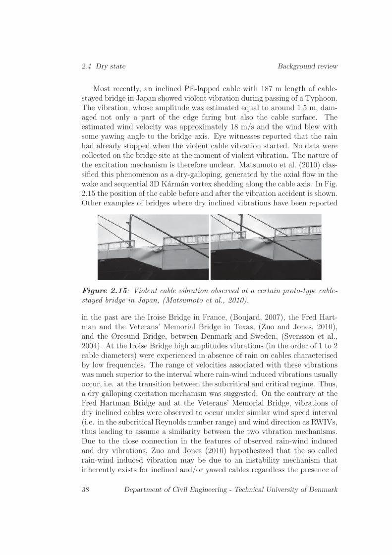
2.4 Dry state Background review
Most recently, an inclined PE-lapped cable with 187 m length of cable-stayed bridge in Japan showed violent vibration during passing of a Typhoon.The vibration, whose amplitude was estimated equal to around 1.5 m, dam-aged not only a part of the edge faring but also the cable surface. Theestimated wind velocity was approximately 18 m/s and the wind blew withsome yawing angle to the bridge axis. Eye witnesses reported that the rainhad already stopped when the violent cable vibration started. No data werecollected on the bridge site at the moment of violent vibration. The nature ofthe excitation mechanism is therefore unclear. Matsumoto et al. (2010) clas-sified this phenomenon as a dry-galloping, generated by the axial flow in thewake and sequential 3D Karman vortex shedding along the cable axis. In Fig.2.15 the position of the cable before and after the vibration accident is shown.Other examples of bridges where dry inclined vibrations have been reported
Figure 2.15: Violent cable vibration observed at a certain proto-type cable-stayed bridge in Japan, (Matsumoto et al., 2010).
in the past are the Iroise Bridge in France, (Boujard, 2007), the Fred Hart-man and the Veterans’ Memorial Bridge in Texas, (Zuo and Jones, 2010),and the Øresund Bridge, between Denmark and Sweden, (Svensson et al.,2004). At the Iroise Bridge high amplitudes vibrations (in the order of 1 to 2cable diameters) were experienced in absence of rain on cables characterisedby low frequencies. The range of velocities associated with these vibrationswas much superior to the interval where rain-wind induced vibrations usuallyoccur, i.e. at the transition between the subcritical and critical regime. Thus,a dry galloping excitation mechanism was suggested. On the contrary at theFred Hartman Bridge and at the Veterans’ Memorial Bridge, vibrations ofdry inclined cables were observed to occur under similar wind speed interval(i.e. in the subcritical Reynolds number range) and wind direction as RWIVs,thus leading to assume a similarity between the two vibration mechanisms.Due to the close connection in the features of observed rain-wind inducedand dry vibrations, Zuo and Jones (2010) hypothesized that the so calledrain-wind induced vibration may be due to an instability mechanism thatinherently exists for inclined and/or yawed cables regardless the presence of
38 Department of Civil Engineering - Technical University of Denmark

Background review 2.4 Dry state
rainfall. The role of rainfall is thus to promote the inherent instability of dryinclined cables exposed to wind loading. Zuo and Jones (2010) claimed alsothat some of the characteristics shared by large amplitude vibrations withand without rainfall are also similar to the corresponding characteristics ofKarman-vortex induced vibrations. At the Øresund Bridge large amplitudevibrations were observed in absence of rain and ice during the life time ofthe bridge by Svensson et al. (2004). Macdonald and Larose (2006) statedthat during these episodes the stay cables might have experience dry inclinedgalloping excitation as the measured wind speed, i.e. in the range of 12 to 21m/s, likely corresponds to the critical Reynolds number, for the given cablesdiameter, i.e. 250 mm, turbulence intensity of the wind at the cable locationand surface roughness of the cables.
2.4.2 Dynamic wind tunnel tests
Dry inclined galloping excitation has been observed in wind tunnel testsconducted in Japan, (Matsumoto et al., 1990), (Saito et al., 1994), (Hondaet al., 1995), (Miyata et al., 1994b), in Canada (Cheng et al., 2003), (Chenget al., 2008a), (Cheng et al., 2008b), (Jacobsen et al., 2012), and in Denmark,(Matteoni and Georgakis, 2013a).
In the experimental investigations, undertaken by Matsumoto et al. (1990),bridge cables were modelled by means of cylinders with scaled diameter andweight with respect to real prototypes. It was observed that both horizon-tal and inclined cylinders can be prone to dry instability, depending on theyaw angle. Existence of a secondary axial flow, located in the near wake ofthe cylinder’s axis, was documented, which has the role of interrupting theregular Karman vortex shedding. In fact, as an air curtain or base bleed,or similarly a splitter plate submerged in the wake, the secondary axial flowprevents the fluid interaction between the two separated shear layers, thusgenerating an unsteady inner circulatory flow at the leeward surface of thecylinder. The inner circulatory flow generates a region of significantly lowerpressure, this latter being responsible of activating the excitation, (Mat-sumoto et al., 1990). Fig. 2.16 shows the flow pattern around a yawedcircular cable, obtained by means of a liquid paraffin method and around ahorizontal cylinder with splitter plate submerged in the wake. A similaritywas assumed by Matsumoto et al. (1990) between the axial flow excitationexcitation and the galloping of rectangular cylinders described by Bearmanand Trueman (1972).
In Fig. 2.17 possible unsteady flow patterns around a circular cylindermoving with velocity y in the downwards direction, in different spacial ori-entations are illustrated. In absence of yaw/inclination (a) regular Karman
Department of Civil Engineering - Technical University of Denmark 39

2.4 Dry state Background review
(a) (b)
Figure 2.16: Secondary axial flow on the leeward surface of yawed circularcylinder, (a); inner circulatory flow of a circular cylinder with splitter platein the leeward side, (b), (Matsumoto et al., 1990).
vortex shedding occurs in the wake. When the cylinder is yawed (b), or in-clined/yawed (c), (d) to the flow, the secondary axial flow develops in theleeward side, thus generating the unsteady inner circulatory flow.
Figure 2.17: Unsteady flow pattern around a circular cylinder in differentspacial orientations, (Matsumoto et al., 1990).
Matsumoto et al. (1990) thus concluded that in order to prevent theexcitation, the secondary axial flow need to be suppressed.
Later on, during the period of construction of the Higashi-Kobe cable-stayed bridge in Japan, seen the concern for potential heavy vibrations ofthe cables when excited by wind or by wind and rain, Saito et al. (1994)performed a series of wind tunnel vibration tests on a life-size cable model,identical in weight as the real cables at the mentioned bridge. It was in factsuspected that previous observations of dry inclined cable vibration couldbe attributed to the lower mass of the models in comparison to real cables.Several cable-wind angles for the cable model were tested, i.e. Φ = 30◦, 45◦,
40 Department of Civil Engineering - Technical University of Denmark

Background review 2.4 Dry state
60◦. A stability criterion was established as outcome of the experimentalcampaign, giving the reduced wind velocity Ur associated to the onset ofdivergent motion, i.e.
(Ur)cr = 14√Sc (2.18)
The criterion showed how the wind velocity at which the inclined cable vi-bration takes place does not vary appreciably over a large range of Scroutonnumbers (50 and under), thus implying that dry inclined cable vibrationappears to be difficult to restrain once it has taken place even if the cablestructural damping is increased to some extent, for example by means of adamper. Soon later, Honda et al. (1995) established a similar instability cri-terion, based on wind tunnel tests undertaken on a full scale section modeloriented at a cable-wind angle of 45◦. Experimental results derived by Saitoet al. (1994) and Honda et al. (1995) thus show how the dry instability de-velops for wind velocities in the subcritical Reynolds number range. On theother hand, (Miyata et al., 1994b) observed divergent motion to occur for acable model oriented at the same cable-wind angle (45◦), but for larger windvelocity, i.e. presumably corresponding to the transition between subcriticaland critical Reynolds number range.
The instability criteria for galloping of dry inclined cables reported byjapanese researchers caused serious concern in the design of cable stayedbridges as they implied that dry inclined cables can be excited at relativelylow wind speed, even if their inherent damping is very high. On the otherhand, reality is that many existing stay cables seem to survive without suf-fering this instability, (Cheng et al., 2008a). In order to first confirm thedivergent type of instability for inclined cables and to subsequently verifythe stability criterion established by japanese researchers, an experimentalcampaign was conducted at NRCC Ottawa in Canada. Results are reportedby Cheng et al. (2003), Cheng et al. (2008a), Cheng et al. (2008b). In theexperimental campaign divergent-type motion was observed for a polyethi-lene coated section model, inclined and yawed to the mean wind direction,oriented at a cable-wind angle of 60◦. The cable surface condition was clas-sified as smooth and the inherent structural damping ratio was 0.001, so asto lead to a Scrouton number, i.e. Sc = mδ/(ρD2), equal to 11. Divergentmotion was achieved when the wind velocity reached a value of 32 m/s, i.e.corresponding to the critical range. At this velocity, the amplitude of motionincreased dramatically within a short period of time, leading to a maximumrecorded peak-to-peak amplitude of approximately 1D, where D is the cablediameter. Model’s trajectories were elliptical and showed how the motion de-veloped predominantly along the in-plane direction. It was finally observedthat the generation of the excitation was difficult to reproduce due to strong
Department of Civil Engineering - Technical University of Denmark 41

2.4 Dry state Background review
sensitivity to the test conditions.
In Fig. 2.18, the wind velocity-damping relation for inclined cable ob-tained by japanese researchers is compared to results obtained during thecanadian tests, (Cheng et al., 2008a), these latter identified as Current.
Figure 2.18: Comparison of wind-velocity damping relation for inclinedcable, (Cheng et al., 2008a).
The data presented in Fig. 2.18 implies that the onset conditions ofdivergent type of motion on a dry stay cable are not certain, i.e. it can happenin the subcritical (Saito et al., 1994), (Honda et al., 1995), at transition to thecritical, (Miyata et al., 1994b), or in the the critical Reynolds number range(Cheng et al., 2008a). Recent results derived by Matteoni and Georgakis(2013a) confirmed that dry inclined instability can occur under a wide rangeof Reynolds number. This is due to non uniform distribution of surfaceroughness/shape of the cable. Thus depending on the wind angle-of-attack,the cable might exhibit unstable/stable response to the wind loading.
Properties of the cable models employed in several dynamic experimentaltest campaigns and the onset conditions for instability are summarised inTables 2.9-2.12.
Vortex induced vibration at high reduced velocity was as well repro-duced in experimental studies in Japan, (Matsumoto et al., 2001), in Canada(Cheng et al., 2003), (Cheng et al., 2008a), (Cheng et al., 2008b), and in Italy,(Diana et al., 2008).
Based on experimental evidence, Matsumoto et al. (2001) and Cheng etal. (2008a) suggested that there could be a strong interaction between dry
42 Department of Civil Engineering - Technical University of Denmark

Background review 2.4 Dry state
Table 2.9: Critical geometrical attitude for dry inclined galloping for thecable models tested dynamically in wind tunnels.
θ [◦] β [◦] Φ [◦] Reference60 0 60 Saito et al. (1994)45 0 45 Saito et al. (1994)30 0 30 Saito et al. (1994)0 45 45 Saito et al. (1994)- - 45 Honda et al. (1995)45 45 60 Miyata et al. (1994b)45 45 60 Cheng et al. (2008a)25 60 63.05 Matteoni and Georgakis (2013a)
Table 2.10: Critical geometrical characteristics for dry inclined gallopingfor the cable models tested dynamically in wind tunnels.
D [m] L [m] Reference0.16 9.5 Saito et al. (1994)0.155 - Honda et al. (1995)0.1315 3 Miyata et al. (1994b)0.16 6.7 Cheng et al. (2008a)0.16 3.35 Matteoni and Georgakis (2013a)
Table 2.11: Critical inertial and dynamic properties for dry inclined gal-loping for the cable models tested dynamically in wind tunnels.
m [kg/m] f [Hz] Sc [-] Reference100 0.61 3.2 Saito et al. (1994)- 0.26 10.5 Honda et al. (1995)6.6 1.8 1.7-2.3 Miyata et al. (1994b)60.8 1.4 11 Cheng et al. (2008a)18.4 1.1 0.5 Matteoni and Georgakis (2013a)
inclined galloping and vortex induced vibration at high reduced wind velocity.In particular, Cheng et al. (2008a) stated that both excitation phenomenamight initiate from vortex-induced vibration and as they develop and reachrelatively large amplitudes of vibration, because of the differences in thephysical conditions, such as cable orientation, wind velocity, wind turbulence,the motion would either decay with further increase in the wind velocity orcontinuously grow.
Department of Civil Engineering - Technical University of Denmark 43

2.4 Dry state Background review
Table 2.12: Onset conditions of instability for dry inclined galloping for thecable models tested dynamically in wind tunnels.
Ur [-] Re [-] A/D Reference72 7.23x10⁴ 0.75 Saito et al. (1994)115 4.65x10⁴ - Honda et al. (1995)79 1.81x10⁵ - Miyata et al. (1994b)134 3.3x10⁴ >0.49 Cheng et al. (2008a)
96-143 1.8-2.7x10⁵ >2 Matteoni and Georgakis (2013a)
Cheng et al. (2008a) observed vortex induced vibrations at high reducedwind velocity to occur for a cable model whose longitudinal axis was orientedat 60◦, 45◦ and 35◦ with respect to the wind direction, obtained by a combi-nation of 60◦, 45◦ and 35◦ vertical inclination and 0◦ yaw. Thus the wind wasblowing along the cable axis. The cable model, in terms of length, diameter,mass was identical to the one where Cheng et al. (2008a) observed dry in-clined galloping. Excitation developed for Reynolds number in the range of2−4·105, i.e. in the critical. Maximum amplitudes of vibration were observedto be function of the cable orientation angle and became larger by increasingthe vertical inclination angle. In particular, the recorded maximum ampli-tude amounted respectively to 67, 31 and 21 mm for cables charactersed byvertical inclination (and cable-wind angles) of 60◦, 45◦ and 35◦. A lock-inphenomenon of the vibration direction was observed to occur, i.e. as soon asthe wind velocity increased to that of unstable motion a considerable changein the direction of motion occurs; within the range of instability the direc-tion of motion thus remains constant, and it is characterised by a dominantcross-wind component; once the wind speed is above the unstable range, thecomponent of cross-wind motion would considerably decrease. If the cableis both inclined and yawed to the wind, the predominant motion direction isnot any longer perpendicular to the cable plane and the motion follows anelliptical path.
2.4.3 Static wind tunnel tests
In order to obtain a clearer insight into the instability of dry inclined ca-bles, static wind tunnel tunnel have been performed in the past, mostly inassociation with vibration tests.
Reynolds number, cable-wind angle, and wind angle-of-attack effects areall important in relation to the cable instability, especially in the flow regimeswhere small increments of the mentioned parameters lead to significant changes
44 Department of Civil Engineering - Technical University of Denmark
Background review 2.4 Dry state
to drag and lift forces, (Larose et al., 2003). In fact, depending on the atti-tude of the cable to the flow (i.e. cable wind angle and angle-of-attack), thebehaviour of the separated shear layers that govern the aerodynamic forcesmay vary with the Reynolds number in a different manner from that of acircular cylinder in cross-flow.
Results of an extensive wind tunnel test investigation on the aerodynamicbehaviour of bridge cables in static conditions, oriented perpendicular thewind and in an inclined/yawed configuration, for varying Reynolds numbersand wind angles-of-attack, is presented in Chapter 3. This is based on a studyperformed by Matteoni and Georgakis (2012). The investigation follows sev-eral studies performed in the past, i.e. Schewe (1983), Zdravkovich (1997)(in cross-flow), Bursnall and Loftin (1951), Larose et al. (2003), Larose et al.(2005), Cheng et al. (2008a), to the flow (in inclined/yawed configuration).
In order to give an overview of the static aerodynamic behavior of circularcylinders, brief conclusions of the previous studies are reported here below.
Schewe (1983) measured the steady and unsteady forces of a small-scalecircular cylinder horizontally oriented and perpendicular to the wind. Itwas found that in the critical Reynolds-number range, two discontinuoustransitions exist, which can be interpreted as bifurcations at two criticalReynolds numbers. The transitions are accompanied by critical fluctuations,symmetry breaking (the occurrence of a steady lift) and hysteresis of the flow.In addition, both transitions are coupled with a drop of the drag coefficientvalue and a jump of the Strouhal number. Similar phenomena were observedin the upper transitional region between the super- and the transcriticalReynolds-number ranges.
Larose et al. (2003) performed a series of static wind tunnel tests on a staycable model made of a 89 mm diameter steel tube. Tests were undertakenin smooth flow, i.e. Iu = 0.13%, for Reynolds number between 1 · 105 and6 ·105, i.e. in the range where transition from laminar to turbulent boundarylayer occurs. This is associated with the formation of the one-asymmetricbubble and two-symmetric bubble regimes, accompanied by a sudden drop ofthe drag coefficient, i.e TrBL0 to TrBL2 (Zdravkovich, 1997). Three modelinclinations were tested, i.e. Θ = 90◦, 60◦, 54.7◦. In the reference case,i.e. Θ = 90◦, β = 90◦ (cylinder perpendicular to the wind flow), the TrBL1regime occurs at Reynolds numbers between 3.1 × 10⁵ to 3.5 × 10⁵; in thisrange of Reynolds number the static across-wind force reaches a mean coeffi-cient of 0.8, while the drag coefficient at the same Reynolds was 0.55. Here,a single laminar separation bubble is suspected to occur causing asymmetryin the pressure distribution, while at Reynolds numbers above 3.5× 10⁵ twolaminar separation bubbles are suspected to occur, one on each side of thecylinder, causing the drag to drop further and almost completely eliminating
Department of Civil Engineering - Technical University of Denmark 45

2.4 Dry state Background review
the lift.Matteoni and Georgakis (2012) observed that for a cable model horizon-
tally oriented and perpendicular to the wind (i.e. at Θ = 0◦, β = 90◦,Φ = 90◦), the critical range generally spans from 2.5 × 10⁵ to 3.0 × 10⁵.On the other hand, small scale deviations in the cable surface roughness orshape, can lead to a variation in the critical range, which might span from1.0 × 105 to 3.3 × 10⁵. This behaviour might explain some of the observedaerodynamic instabilities, such as dry inclined galloping. In Table 2.13 aresummarised the range of critical Reynolds number for cylinders in cross flow(Φ = 90◦).
Table 2.13: Range of critical Reynolds number for cross-flow cylinders (Φ =90◦).
Recr [-] Reference1.7× 105-2.5× 10⁵ Schewe (1983)3.1× 10⁵-3.5× 10⁵ Larose et al. (2003)2.5× 10⁵-3.0× 10⁵ Matteoni and Georgakis (2012)
Bursnall and Loftin (1951) measured the pressure distributions on asmooth small-scale brass tube for a series of vertical inclination angles, i.e.Θ = 30◦, 45◦, 60◦, 75◦, 90◦, and zero yaw, β = 0◦, for Reynolds numbersup to 5.0 × 10⁵. Tests were performed in laminar flow, in a low turbulencewind tunnel (0.05%). It was mainly observed that in the subcritical rangethe cylinder’s pressure distributions are quite insensitive to the inclinationangle. On the other hand, a gradual change takes place in the pressure dis-tribution through and beyond the critical range, as the inclination angle isincreased. The laminar separation bubble, which is responsible for asymmet-ric pressure distributions and therefore across-wind forces, does not appearas well defined at Φ = 90◦; on the other hand, it is present at Φ = 75◦ andΦ = 60◦, and completely disappears at Φ = 45◦ and Φ = 30◦. Drag coeffi-cients curves show that the lower is the cable inclination, the earlier is thetransition from subcritical to critical regime, thus producing a similar effectas increased surface roughness or turbulence intensity. Similarily Larose etal. (2003) observed that for an inclined cylinder (Θ = 60◦), the variation ofthe lift coefficient shows that the TrBL1 still exists but it spans over a widerrange of Reynolds number.
Larose et al. (2005) observed that the turbulence intensity of the naturalwind on bridge sites is likey to be much larger in comparison to the smoothflow conditions tested in the past, i.e. corresponding to a wind tunnel tur-bulence intensity below 1%. Moreover, since in field conditions the critical
46 Department of Civil Engineering - Technical University of Denmark

Background review 2.4 Dry state
mean wind speed can be reached either from lower or higher wind regime,a possible hysteresis of the single bubble regime might occur. For this rea-son, Larose et al. (2005) performed a series of wind tunnel tests on a 316mm diameter HDPE tube, for Reynolds numbers spanning the subcritical tothe supercritical range, i.e. 1 × 10⁵ to 3.3 × 10⁵. The cable was installedhorizontally, leading to 0◦ inclination. By changing the yawing angle, cable-wind angles in the range of 20◦ to 85◦ were achieved. Tests were undertakenat turbulence intensities of 2.5% and 11%. As the cable-wind angle wasincreased, the drag coefficient in the subcritical range increased, while thedrag crisis was anticipated. From the lift coefficient curves it was visiblehow the single bubble regime was present over a wider range of yaw angles,(40◦ ≤ β ≤ 85◦), in contrary to the range of (55◦ ≤ β ≤ 65◦) experienced byLarose et al. (2003). The effect of increasing the turbulence intensity up to11% was to completely eliminate the single bubble regime, i.e. the lift curvebecomes flat and close to 0, throughout the whole Re range.
Department of Civil Engineering - Technical University of Denmark 47

2.5 Iced state Background review
2.5 Iced state
Ice accretion is a time-dependent modification of the shape of an object, oc-curring on a longer time scale compared with those of any possible dynamicresponse. Atmospheric icing occurs in different forms, i.e. hoar frost, causedby the condensation of vapour, in-cloud icing, involving the freezing of super-cooled water droplets in clouds or fog, and precipiation icing, resulting fromfreezing rain, drizzle, wet snow or dry snow, Farzaneh (2008). The role of iceaccretion on the aerodynamic instability of bridge cables has been recognisedin the recent years. Nevertheless, a clear systematization of the knowledgeon this form of instability doesn’t exist, as neither field monitoring data nordynamic wind tunnel test data have been collected. Static measurements ofthe aerodynamic drag, lift and moment coefficients of full-scale bridge cablesections have instead been performed recently in Denmark, (Koss and Mat-teoni, 2011), (Koss and Lund, 2013), (Demartino et al., 2013), (Demartinoet al., 2013).
2.5.1 Field observations
As for the dry state, field monitoring data of bridge cable sections coveredby ice accretions are scarce.
Records of cable vibrations in freezing conditions have been reported forbridges in the Northern Hemisphere, such as the Øresund bridge, locatedbetween Denmark and Sweden, (Svensson et al., 2004), the Great Belt Eastbridge in Denmark, (Gjelstrup et al., 2007), the Uddevalla Bridge in Sweden,(Vincentsen and Lundhus, 2006), the Severn Bridge in UK, (Vincentsen andLundhus, 2006), the Zakim Bunker Hill Bridge, in USA, and the HukahoBridge, in Japan, (Gimsing and Georgakis, 2012). Besides vibration, episodesof cable icing might represent a safety problem for the bridge users, due tothe phenomenon of ice shedding.
The Great East Belt Bridge was closed for several hours in March 2001,after the occurrence of large amplitude vibrations of the bridge hangers. Thevibrations occurred for wind velocities in the range of 16-18 m/s and werecharacterised by amplitudes in the order of 2 m in the across-wind directionand in the order of 0.6 m in the along-wind direction, (Gjelstrup et al., 2007).
Several icing events were reported at the Toledo Skyway Bridge, in Ohiosince its opening, (Nims, 2011). Figs. 2.19 show icing accumulations on thestays occurred on December 2007. It was reported that for this occurrencethe wheather conditions causing the ice accumulation were characterised byfreezing rain and fog. The bridge cable’s sheat is made of stainless steel, witha brushed finish, and it lacks a helical spire. So far, no anti-icing systems
48 Department of Civil Engineering - Technical University of Denmark

Background review 2.5 Iced state
have been installed at the bridge stays.
(a) (b)
(c)
Figure 2.19: Ice hanging on the stay sheat (a); patter of ice release (b); icefallen from the stays to the deck (c) at Toledo Skyway Bridge, in Ohio onDecember 2007, (Nims, 2011).
Fig. 2.20 shows an overview of ice accretion occurred at the Toledo Sky-way Bridge later in February 2011. The wheather conditions causing thisevent were again characterized by freezing rain.
In December 2012 the Portman Bridge in Vancouver, British Columbia,was closed for several hours after snow and ice falling from the supportingcables, causing injure to two people and dozen of vehicles. Fig. 2.21 showsa detail of the iced cable sections at the bridge.
In order to prevent snow and ice to fall on the bridge deck, sweepers werecustom-designed to be fitted around the cables on the Port Mann Bridge.Fig. 2.22 shows a prototype of the sweepers.
2.5.2 Dynamic wind tunnel tests
Dynamic wind tunnel tests have not been performed so far on bridge cablesections. Thus the characteristics of the instability are still unclear.
Department of Civil Engineering - Technical University of Denmark 49

2.5 Iced state Background review
(a) (b)
(c)
Figure 2.20: Overview (a) and close-up (b) of ice accumulation under freez-ing rain on the stays at Toledo Skyway Bridge, in Ohio on February 2011;diagramm of ice accumulation (c), (Nims, 2011).
(a) (b)
Figure 2.21: Ice formations on the cable sections at the Port Mann Bridgein Vancouver, British Columbia (a); damage on a passing car (b). (Picturesfrom http://www.vancouversun.com/).
On the other hand, few experimental wind tunnel dynamic investigationshave been undertaken for cable conductors covered by ice accretion, for ex-ample by Chabart and Lilien (1998). It is nevertheless unclear whether the
50 Department of Civil Engineering - Technical University of Denmark

Background review 2.5 Iced state
Figure 2.22: Custom-designed ice/snow sweepers to be fitted to the staysat the Portmann Bridge in Vancouver, British Columbia. (Pictures fromhttp://www.news1130.com/).
results of such tests are directly applicable to bridge cable sections. In fact,the ratio between the size of the accretion and the conductor diameter ismuch higher than for a full-scale cable. The same applies for the associatedmass ratios.
2.5.3 Static wind tunnel tests
Few wind tunnel tests have been performed in order to understand the in-stability of iced bridge cables. Koss et al. (2012) investigated, by performinga series of wind tunnel tests at NRC Canada, the characteristic shapes of iceaccretions on circular cylinders under the specific climatic conditions wherelarge amplitude vibrations of iced birdge cables have been observed in na-ture. In particular with reference to the episodes occurred at the Great EastBelt (Gjelstrup et al., 2007). This study was followed by a long and still on-going test campaign at the novel climatic wind tunnel recently constructedin Denmark,(Georgakis et al., 2009). The facility was specifically built forthe purpose of testing bridge cable sections under variable flow and climaticconditions, in particular conditions related to low altitude atmospheric ic-ing. Investigations have been performed on the aerodynamic coefficients ofcross-flow horizontal, (Koss and Matteoni, 2011), (Koss and Lund, 2013)and vertical, (Demartino et al., 2013) bridge cables and inclined/yawed tothe wind, (Demartino et al., 2013).
Koss and Lund (2013) studied in detail the features of ice accretion for ahorizontally installed bridge cable. These are illustrated in Fig. 2.23. In anearly stage of the accretion rime ice accumulates along the cable’s stagnationline, which appears as a smoother core zone (a); curved jagged ice structuresstart later to grow towards the flow stagnation line resembling the appearence
Department of Civil Engineering - Technical University of Denmark 51

2.6 Conclusion Background review
of feathers until they reach a limit near the stagnation line (b); dependingon the temperature and on the liquid water content of the air some flow-outaccumulations might develop, (c) and (d).
Figure 2.23: Description of the ice accretion features, (Koss and Lund,2013).
Koss and Lund (2013) and Demartino et al. (2013) additionally deter-mined the drag and lift coefficients for varying Reynolds number and angles-of-attack of horizontal and vertical iced cables respectively, under conditionsof wet and dry ice accretion. The coefficients were employed in the classicalDen Hartog 1 DOF critierion in order to predict the regions of gallopinginstability.
Force coefficients of inclined/yawed cable sections have been determinedby Demartino et al. (2013). In this study the ice accretion was performedfor selected orientations of the cable model with respect to the wind. Afterthe accretion process was ultimated the force coefficients were evaluated forvarying Reynolds numbers and for a series of cable-wind angles, obtained bychanging the yaw angle of the cable and keeping the same inclination as theone adopted during the accretion process. Investigation of the dependencyof the force coefficients on the wind-angle-of-attack for varying cable-windangles and Reynolds numbers could instead be a topic of future research, asit was not investigated into details in this study.
2.6 Conclusion
Bridge cables are classified as bluff bodies and as such can only undergoinstabilities of vortex shedding-, buffeting- and galloping-type. Depending
52 Department of Civil Engineering - Technical University of Denmark

Background review 2.6 Conclusion
on the climatic conditions they are subjected to, the characteristics of suchinstabilities differ significantly.
A literature review on the different excitation mechanisms of inclinedcables under varying meteorological conditions, i.e. in the dry, rainy andiced state, was here given. The review was based on the most recent find-ings achieved from full scale monitoring, wind tunnel testing and theoreticalmodelling.
Systematization of the current knowledge leaded to conclude that:
• Rain-wind induced is a limited amplitude-type instability, occurringover a restricted range of wind velocities, under moderate rain condi-tions, for cables descending in the wind direction. The instability wasmostly observed for plain surfaced cables, coated with polyethylene(PE), where the water rivulet could easily form, under the achieve-ment of the right level of surface wettability. This form of instabilityhas been observed both on full-scale and in wind tunnel tests, and a fairagreement in the characterization of the excitation mechanism, basedon the two approaches, has been achieved.
• In dry conditions, two types of excitation have been recognised. Undera combination of parameters, such as cable attitude to the flow, windvelocity, stay cables may either undergo divergent motion (dry gallop-ing) or limited amplitude motion under a limited interval of wind speed(vortex induced vibration at high reduced wind speed). Dry cable vi-brations have been observed only in wind tunnel experimental studies,while they have never been fully verified on full-scale bridges.
• Instability of bridge cables in the iced state has been recognised as aform of galloping. The aerodynamic force coefficients of perpendicularand inclined/yawed full-scale bridge cables covered by ice accretionshave been determined by performing static wind tunnel tests. On theother hand a complete characterization of the iced state instability,based on passive-dynamic wind tunnel tests and full-scale monitoringhas never been performed.
Department of Civil Engineering - Technical University of Denmark 53

2.6 Conclusion Background review
54 Department of Civil Engineering - Technical University of Denmark

Bibliography
Acampora, A., Georgakis, C.T., 2011. Recent monitoring of the ØresundBridge: Observations of rain-wind induced cable vibrations. In: 13th In-ternational Wind Engineering Conference, Amsterdam.
Alam, MD., Zhou, Y., 2007. Turbulent wake of an inclined cylinder withwater running. J. Fluid Mech. 589, 261-303.
Bearman, P.W., Trueman, D.M., 1972. An investigation of the flow aroundrectangular cylinders. The Aeronatical Quarterly, 23.
Benedir, A., Flamand, O., Gaillet, L., Dimitriadis, G., 1972. Dry gallopingon bridge cables: Shape effects on an inclined circular cylinder in thewind tunnel. In: 6th European African Conference Wind Engineering,Cambridge.
Bosdogianni, A., Olivari, D., 1996. Wind-and rain-induced oscillations ofcables of stayed bridges. J. Wind Eng. Ind. Aerodyn. 64, 171-185.
Boujard, O., 1996. Wind-and rain-induced oscillations of cables of stayedbridges. J. Wind Eng. Ind. Aerodyn. 64, 171-185.
Bursnall, W.J., Loftin, L.K., 1951. Experimental investigation of the pres-sure distribution about a yawed circular cylinder in the critical Reynoldsnumber range. Technical report, Langley Aeronautical Laboratory, Lang-ley Field, Va.
de Sa Caetano, E., 2007. Cable Vibrations in Cable-Stayed Bridges. Interna-tional Association for Bridge and Structural Engineering.
Chabart, O., Lilien J.L., 1998. Galloping of electrical lines in wind tunnelfacilities. J. Wind Eng. Ind. Aerodyn. 74-76, 967-976.
Cheng, S., Larose, G.L., Savage, M.G., 2003. Aerodynamic behaviour of aninclined circular cylinder. J. Wind and Structures 6 (3), 197-208.
55

BIBLIOGRAPHY BIBLIOGRAPHY
Cheng, S., Larose G.L., Savage, M., Tanaka, H., Irwin, P.A., 2008a. Experi-mental study on the wind-induced vibration of a dry inclined cable - PartI: Phenomena. J. Wind Eng. Ind. Aerodyn. 96 (12), 2231-2253.
Cheng, S., Irwin P.A., Tanaka, H., 2008b. Experimental study on the wind-induced vibration of a dry inclined cable - Part II: Proposed mechanisms.J. Wind Eng. Ind. Aerodyn. 96 (12), 2254-2272.
Clobes, M., Steiln, O.., Peil, U., 2010. Aerodynamic force coefficients forrain-wind induced vibrations from full-scale measurements. In: 5th Inter-national Conference on Structural Engineering, Mechanics and Computa-tion.
Collar, A., 1978. The first fifty years of aeroelasticity. Aeroespace, RoyalAeronautical Society, vol. 545.
Cosentino, N., Flamand, O., Ceccoli, C., 2003. Rain-wind-induced vibrationof inclined stay cables. Part I: experimental investigation and physicalexplanation. Wind Struct. 6, 471-484.
Davenport, A.G., 1962. Buffeting of a suspension bridge by storm winds. J.Struct. Division ASCE, 88-3, 233-268.
Demartino, C., Koss, H.H., Ricciardelli, F., 2013. Experimental study of theeffect of icing on the aerodynamics of circular cylinders - Part I: Cross flow.In: 6th European African Conference Wind Engineering, Cambridge.
Demartino, C., Georgakis, C.T., Ricciardelli, F., 2013. Experimental studyof the effect of icing on the aerodynamics of circular cylinders - Part II:Inclined flow. In: 6th European African Conference Wind Engineering,Cambridge.
Den Hartog, J.P., 1958. Mechanical vibrations. Courier Dover Publications
Diana, G., Belloli, M., Giappino, S., Muggiasca, S., 2008. Vortex inducedvibrations at high Reynolds numbers. In: 7th International Colloquium onBluff Bodies Aerodynamics and Applications, Milano, Italy.
Ehsan, F., Scanlan, R.H., Bosch, H.R., 1990. Modeling spanwise correctioneffects in the vortex-induced response of flexible bridges. J. Wind Eng. Ind.Aerodyn. 36 (2), 1105-1114.
Farzaneh, M., 2008. Atmospheric icing of power networks. Springer.
56 Department of Civil Engineering - Technical University of Denmark

BIBLIOGRAPHY BIBLIOGRAPHY
Flamand, O., 1995. Rain-wind induced vibration of cables. J. Wind Eng. Ind.Aerodyn. 57, 353-362.
Flamand, O., Peube, J.-L., Papanikolas, P., 2001. An explanation of the rain-wind induced vibration of inclined stays. In: IV International Symposiumon Cable Dynamics, Montreal, Canada, May 28-30, pp. 69-76.
Fujino, Y., Kimura, K., Tanaka, H., 2012. Wind Resistant Design of Bridgesin Japan. Springer.
Georgakis, C.T., Koss, H.H., Ricciardelli, F., 2009. Design specifications fora novel climatic wind tunnel for testing of structural cables. In: 8th Inter-national Symposium on Cable Dynamics, Paris, pp. 333-340.
Gimsing, N.J., Georgakis, C.T., 2012. Cable Supported Bridges. Concep andDesign. Third Edition. Wiley.
Gjelstrup, H., Georgakis, C.T., Larsen, A., 2007. A preliminary investigationof the hanger vibrations on the Great Belt East Bridge. In: VII Interna-tional Symposium on Cable Dynamics, Vienna, pp. 469-476.
Gjelstrup, H., Georgakis, C.T., 2011. A quasi-steady 3 degree-of-freedommodel for the determination of the onset of bluff body galloping instability.In: Journal of Fluids and Structures, 27 (7), 1021-1034.
Gu, M., Du, X., 2005. Experimental investigation of rain-wind-induced vi-bration of cables in cable-stayed bridges and its mitigation. J. Wind Eng.Ind. Aerodyn. 93, 79-95.
Gu, M., Huang, L., 2008. Theoretical and experimental studies on the aero-dynamic instability of a two-dimensional circular cylinder with a movingattachment. J. Fluids and Structures 24, 200-211.
Hikami, Y., Shiraishi, N., 1988. Rain-wind induced vibrations of cables stayedbridges. J. Wind Eng. Ind. Aerodyn. 29, 409-418.
Hardy, C., Bourdon, P., 1979. The influence of spacer dynamic propertiesin the control of bundle conductor motion. IEEE PES Summer Meeting,Vancouver, British Columbia, Canada
Honda, A., Yamanaka, T., Fujiwaraa, T., Saito, T.,1995. Wind tunnel test onRain-Induced Vibration of the Stay Cable. In: International Symposiumon Cable Dynamics, Liege, Belgium, pp. 255-262.
Department of Civil Engineering - Technical University of Denmark 57

BIBLIOGRAPHY BIBLIOGRAPHY
Irwin, P.A., Nedim, A., Telang, N., 1999. Wind induced stay cable vibrationsa case study. In: 3rd International Symposium on Cable Aerodynamics,Trondheim, Norway, pp. 171-176.
Jacobsen, J.B., Andersen, T.L., Macdonald, J.H.G., Nikitas, N., Larose,G.L., Savage, M.G., McAuliffe, B.R., 2012. Wind-induced response andexcitation characteristics of an inclined cable model in the critical Reynoldsnumber range. J. Wind Eng. Ind. Aerodyn. 110, 100-112.
Koss, H.H., Matteoni, G., 2011. Experimental investigation of aerodynamicloads on iced cylinders. In: 9th International Symposium on Cable Dy-namics, Shanghai, 381-388.
Koss, H.H., Gjelstrup, H., Georgakis, C.T., 2012. Experimental study of iceaccretion on circular cylinders at moderate low temperatures. J. Wind Eng.Ind. Aerodyn. 104-106, 540-546.
Koss, H.H., Lund Møller, M.S., 2013. Experimental Investigation of Aerody-namic Instability of Iced Bridge Cable Sections. In: 6th European AfricanConference Wind Engineering, Cambridge.
Langsoe, H.E., Larsen, O.D., 1987. Generating mechanisms for cable stayoscillations at the Faroe Bridge. In: Int. Conf. on Cable-stayed Bridges,Bangkok, pp. 18-20.
Larose, G.L., Smitt, L.W., 1999. Rain/wind induced vibrations of the parallelstay cables for the Oresund High Bridge. In: IABSE Conference, Malmo,June, pp. 1-12.
Larose, G.L., Savage, M.G., Jakobsen, J.B., 2003. Wind tunnel experimentson an inclined and yawed circular cylinder in the critical Reynolds numberrange. In: 11th International Conference on Wind Engineering, Lubbock.
Larose, G.L., Zasso, A., Giappino, S., 2005. Experiments on a yawed staycable in turbulent flow in the critical Reynolds number range. In: 6thInternational Symposium Cable Dynamics, Charleston, pp. 279-286.
Liu, Q., Wang, Y., Zheng, Y.,Ma, W., 2012. Experimental study on therelation of water rivulet-Reynolds number effect-cable vibration. In: 7thInternational Colloquium on Bluff Body Aerodynamics and Applications,Shanghai, China.
Macdonald, J.HJ., Larose G.L., 2008a. A unified approach to aerodynamicdamping and drag/lift instabilities, and its application to dry inclined cablegalloping. J. Fluids Struct. 22, 229-252.
58 Department of Civil Engineering - Technical University of Denmark

BIBLIOGRAPHY BIBLIOGRAPHY
Main, J.A., Jones, N.P., Yamaguchi, H., 2001. Characterization of rain-windinduced stay-cable vibrations from full-scale measurements. In: FourthInternational Symposium on Cable Dynamics, Montreal, Canada, pp. 235-242.
Matsumoto, M., Shiraishi, N., Kitazawa, M., Knisely, C., Shirato, H., Kim,S., Tsujii, M., 1990. Aerodynamic behaviour of inclined circular cylinders-Cable aerodynamics. J. Wind Eng. Ind. Aerodyn. (33), 63-72.
Matsumoto, M., Shiraishi, N., Shirato, H., 1992. Rain-wind induced vibrationof cables of cable-stayed bridges. J. Wind Eng. Ind. Aerodyn. 43, 2011-2022.
Matsumoto, M., Saitoh, T., Kitazawa, M., Shirato, H., Nishizaki, T., 1995.Response characteristics of rain-wind induced vibration of stay cables ofcable-stayed bridges. J. Wind Eng. Ind. Aerodyn. 57, 323-333.
Matsumoto, M., Yagi, T., Tsushima, D., 1999. Vortex-induced vibration ofinclined cables at high wind velocity. In: 10th International Conference onWind Engineering, Copenhagen, pp. 979-986.
Matsumoto, M., Yagi, T., Shigemura, Y., Tsushima, D., 2001. Vortex-induced cable vibration of cable-stayed bridges at high reduced wind ve-locity. J. Wind Eng. Ind. Aerodyn. 89 (7-8), 633-647.
Matsumoto, M., Shirato, H., Yagi, T., Goto, M., Sakai, S., Ohya, J., 2003.Field observation of the full-scale wind-induced cable vibration. J. WindEng. Ind. Aerodyn. 91, 13-26.
Matsumoto, M., 2005. The role of water rivulet on inclined cable aerody-namics. In: 6th Asia-Pacific Conference on Wind Engineering, Seoul, pp.63-77.
Matsumoto, M., 2006. Review of Bridge Cable Vibrations in Japan. Thepractical Cases of Aerodynamic Vibration of Stayed Cables. Wind InducedVibration Cable Workshop, April 25-27.
Matsumoto, M., Yagi, T., Hatsuda, H., Shima, T., Tanaka, M., Naito, H.,2010. Dry galloping characteristics and its mechanism of inclined/yawedcables. J. Wind Eng. Ind. Aerodyn. 98, 317-327.
Matteoni, G., Georgakis, C.T., 2013. Effects of bridge cable surface roughnessand cross-sectional distortion on aerodynamic force coefficients. J. WindEng. Ind. Aerodyn., 104-106, 176-187.
Department of Civil Engineering - Technical University of Denmark 59

BIBLIOGRAPHY BIBLIOGRAPHY
Matteoni, G., Georgakis, C.T., 2013. Effects of surface roughness and cross-sectional distortion on the wind-induced response of bridge cables in dryconditions, submitted to the J. Wind Eng. Ind. Aerodyn.
Matteoni, G., Georgakis, C.T., 2013. Effects of surface and inertial propertiesof bridge cables on the rain-wind induced instability, submitted to the J.Wind Eng. Ind. Aerodyn.
Miyata, T., Yamada, H., Hojo, T.,1994b. Aerodynamic response of PEstay cables with pattern-indented surface. In: Proceedings of the Inter-national Conference A.I.P.C.-F.I.P. Deauville on Cable-stayed and Sus-pension Bridges, Vol. 2, pp. 515-522.
Miyata, T., 2003. Historical view of long-span bridge aerodynamics. J. WindEng. Ind. Aerodyn. 91, 1393-1410.
Nebres, J., Batill, S., 1993. Flow about a circular cylinder with a singlelarge-scale surface perturbation. Exps. Fluids 15, 369-379.
Ni, Y.Q., Wang, X.Y., Chen, Z.Q., Ko, J.M., 2007. Field observations ofrain-wind-induced cable vibration in cable-stayed Dongting Lake Bridge.J. Wind Eng. Ind. Aerodyn. 95, 303-328.
Nims, D., 2011. Ice Prevention or Removal on the Veteran’s Glass City Sky-way Cables. Interim Report.
Ohshima, K., Nanjo, M., 1987. Aerodynamic Stability of the Cables of aCable-Stayed Bridge Subject to Rain (A Case History of the AjigawaBridge). In: 3rd US-Japan Bridge Workshop, Tsukuba, Japan.
Persoon, A.J., Noorlander, K., 1999a. Full-scale measurements on the Eras-mus Bridge after rain/wind induced cable vibrations. In: Larsen, A.,Larose, G.L., Livesey, F.M. (Eds.), Wind Engineering into the 21st Cen-tury.
Peil, U., Dreyer, O., 2007. Rain-wind induced vibrations of cables in laminarand turbulent flow. Wind and Structures 10, 83-97.
Robertson, A.C., Taylor, I.J., 2007. Effect of rivulets on a circular cylinderunsing a 2D discrete vortex method. In: 12th International Conference onWind Engineering, Cairns, Australia, pp. 863-870.
60 Department of Civil Engineering - Technical University of Denmark

BIBLIOGRAPHY BIBLIOGRAPHY
Saito, T., Matsumoto, M., Kitazawa, M., 1994. Rain-wind excitation of cableson cable-stayed Higashi-Kobe Bridge and cable vibration control. In: In-ternational Conference on Cable-Stayed and Suspension Bridges (AFPC),vol. 2. Deauville, France, pp. 507-514.
Schewe, G., 1983. On the force fluctuations acting on a circular cylinder incrossflow from subcritical up to transcritical Reynolds number. J. FluidMech., 133, 265-285.
Scruton, C., 1963. Introductory review of wind effects on buildings and struc-tures. In: 1st International Conference Wind Engineering, Teddington.
Solari, G., 1994. Gust-excited vibrations. In: Wind-excited vibrations ofstructures, Sockel, H., Ed. Springer Verlag, Wien, 195-291.
Strømmen, E., 2010. Theory of Bridge Aerodynamics. Third Edition,Springer.
Svensson, B., Emmanuelsson, L., Svensson, E., 2004. Oresund Bridge-Cablesystem. Vibration incidents, mechanisms and alleviating measures. In 4thInternational Cable Supported Bridge Operators Conference, Copenhagen,pp. 99-108.
Tubino, F., 2005. Relationships among aerodynamic admittance functions,flutter derivatives and static coefficients for long span bridges. J. WindEng. Ind. Aerodyn. 93, 929-950.
Van der Hoven, I., 1957. Power spectrum of wind velocity fluctuations inthe frequency range from 0.0007 to 900 cycles per hour. J. Meteor, 14,1254-1255.
Verwiebe, C., Ruscheweyh, H., 1998. Recent research results concerning theexciting mechanisms of rain-wind induced vibration. J. Wind Eng. Ind.Aerodyn., 74-76, 1005-1013.
Vincentsen, L.J., Lundhus, P., 2007. The Øresund and the Great Belt linksExperience and Developments. In: IABSE Symposium Report, 93 (30),pp. 1-8.
Wang, Z.J., Zhou, Y., Huang, J.F., Xu, Y.L., 2005. Fluid dynamics aroundan inclined cylinder with running water rivulets. J. of Fluid and Structures21, 49-64.
Virlogeux, M. Cable vibrations in cable-stayed bridges. In: Bridge Aerody-namics, Balkema, 213-233.
Department of Civil Engineering - Technical University of Denmark 61

BIBLIOGRAPHY BIBLIOGRAPHY
Wagner, P., Fuzier, J.P., 2003. Health monitoring of structures-which so-lutions. Dissemination of the results of the IMAC European Project. In:5th Int. Symposium on Cable Dynamics, Santa Margherita Ligure, pp.333-340.
Wianecki, J., 1979. Cables wind excited vibrations of cable-stayed bridges.In: 5th Int. Conf. of Wind Eng., Colorado, Oxford-New York, PergamonPress, pp. 1381-1393.
Xu, L.S., Ge, Y.J., Zhao, L., 2009. Experimental investigation of rain-wind-induced vibration of stay cables based on high precision raining machine.In: The Seventh Asia-Pacific Conference on Wind Engineering, Taipei,Taiwan.
Yamaguchi, H., 1990. Analytical study on the growth mechanism of rainvibration of cables. J. Wind Eng. Ind. Aerodyn. 33, 78-80.
Yoshimura, K., Tanaka, C., Sasaki, N., Nakatani, S., Higa, S., 1988. Rain-Wind Induced vibration of the cables of the Aratsu Bridge. In: 10th Na-tional Symposium on Wind Engineering, pp. 127-132.
Zdravkovich, 1997. Flow around circular cylinders. Volume 1: Fundamentals.Oxford University Press.
Zhan, S., Xu, Y.L., Zhou, H.J., Shum, K.M., 2008. Experimental study ofwind-rain-induced cable vibration using a new model setup scheme. J.Wind Eng. Ind. Aerodyn. 96, 2438-2451.
Zuo, D., Jones, N., Main, J., 2008. Field observation of vortex- and rain-wind-induced stay-cable vibrations in a three-dimensional environment. J.Wind Eng. Ind. Aerodyn. 96, 1124-1133.
Zuo, D., Jones, N., 2010. Interpretation of field observations of wind- andrain-wind-induced stay cable vibrations. J. Wind Eng. Ind. Aerodyn. 98,73-87.
62 Department of Civil Engineering - Technical University of Denmark

Chapter 3
Static wind tunnel tests
The results presented in this chapter are taken from the paper Effects ofbridge cable surface roughness and cross-sectional distortion on aerodynamicforce coefficients, G. Matteoni, C.T. Georgakis, published in the Journal ofWind Engineering and Industrial Aerodynamics 2012, (104-106) 176-187.
Abstract
Theoretical and experimental investigations to date have assumed that bridgecables can be modelled as ideal circular cylinders and the associated aerody-namic coefficients are invariant with the wind angle-of-attack. On the otherhand, bridge cables are normally characterized by local alterations of theirinherent surface roughness and shape, which might present a significant dis-turbance for the surrounding wind flow. The present study focuses on theexperimental determination, based on static wind tunnel tests, of the aerody-namic coefficients of full-scale bridge cable section models both perpendicularand inclined to the flow, for varying wind angles-of-attack. The wind tunneltest results demonstrate that the aerodynamic coefficients of bridge cablescan be significantly affected by the wind angle-of-attack.
3.1 Introduction
When modeling bridge cables for theoretical and experimental investigations,they are often assumed to be perfectly circular cylinders, belonging to a classof bodies which are termed semi-aerodynamic. In contrast to aerodynamicbodies, such as airfoils, which avoid flow separation, and non-aerodynamicbodies with sharp edges, such as squares, which have fixed flow separations
63

3.1 Introduction Static wind tunnel tests
at some of the corners, for semi-aerodynamic bodies the position of the sep-aration point varies depending on the free-stream velocity, turbulence inten-sity and flow profile, and the geometry and roughness of the body’s surface,(Niemann and Holscher, 1990). For disturbance-free and ideal 2D flow con-ditions, the Reynolds number is the governing parameter of the transitionswhich occur in the disturbed regions of the flow around a circular cylinder,i.e. the wake, in the shear layer and the boundary layer. The lower andupper limits of the Reynolds numbers where such transitions occur showconsiderable hysteretic effects which depend on whether the flow velocity isincreased or decreased, (Zdravkovich, 1997). On the other hand, real flowsaround actual cylindrical structures, such as bridge cables, are affected bya wide variety of surface disturbances and shape deviations, which are non-uniformly distributed along their surface. High density polyethylene (HDPE)tubing is commonly used to cover the steel strands or wires of bridge cables.The tubing might be expected to exhibit local alterations of its inherentsurface roughness, resulting from mechanical damage and exposure to theelements, i.e. atmospheric pollution, the sun and water. Changes in thesurface roughness may also augment a cable’s wettability and lead to orenhance rain-wind induced vibrations, (Flamand, 1995). Furthermore, thecross-sectional shape of the HDPE tubing usually deviates from an ideal cir-cular cylinder, as cross-sectional distortions are first introduced during themanufacturing process and later due to the rolling or stacking of the tubingfor transportation and long-term creep. Flow disturbances can initiate tran-sitions at lower Reynolds numbers and sometimes may significantly modifythe resulting flow structures (Zdravkovich, 2003), i.e. microscopic changeson the body’s surface can provoke macroscopic changes in the flow aroundit, (Schewe, 1983).
The critical state or transition-in-boundary layer state, as identified byZdravkovich (1997), has attracted most research attention, since it is in thisrange of Reynolds numbers that significant changes in the aerodynamic co-efficients, provoked by changes in the flow structure, are occurring and thusconditions for potential instability are set. In particular, two discontinuousflow transitions, accompanied by symmetry breaking of the flow field, andhysteresis, have been observed, which are interpreted as bifurcations at twocritical Reynolds numbers (Schewe, 1983). In the first transition, a bi-stableasymmetric flow state occurs, characterized by a first drop in the drag coef-ficient and the simultaneous appearance of a steady lift. The state is calledbi-stable, because - if the cylinder’s surface is free from disturbances - thereare two possible stable states corresponding to either a positive or a nega-tive lift force. The asymmetric flow and the related steady lift are causedby rapid transition to turbulence in the separated boundary layer and sub-
64 Department of Civil Engineering - Technical University of Denmark

Static wind tunnel tests 3.1 Introduction
sequent reattachment to the cylinder’s surface. Thus, a closed flow regionbetween separation and re-attachment, called separation bubble, is formed.The span wise bubble formation may thus take place on either side of thecylinder, but once established it can not change side, due to the lengtheningof the boundary layer on the bubble side, which stabilizes the bubble, andthe shortening of the boundary layer on the opposite side, which precludesthe formation of the second separation bubble. The concept of bi-stable flowis on the other end an idealization, since in practical cases, such as in bridgecables, the cylinder’s surface as seen from the flow is never perfectly sym-metric. Small perturbations or surface disturbances thus affect the locationof the separation bubble and the sign of the lift force (Schewe, 1986). Forexample, a microscopic change in cylinder shape may result in accelerationof the fluid on the side where the boundary layer transition has occurred anddeceleration on the other side of the cylinder. Furthermore, early studiesperformed on partially roughened cylinders, showed also that the presenceof local disturbances on the body’s surface has the smallest effect on thestructure of the flow when distributed in the stagnation region, and in therear surface region. In contrast, the flow is particularly sensitive to local sur-face roughness distributed on the remaining part of the cylinder, i.e. on thecritical region, where boundary layer separation is expected to occur (Fageand Warsap, 1929). The second transition is associated with a second dropin the drag coefficient, to almost half its subcritical value, together with theabrupt disappearance of the steady lift. The transition occurs after reattach-ment of the boundary layer on the back of the cylinder and the appearanceof a second separation bubble on the opposite side of the cylinder. Here, asymmetrical flow state is re-established. On the other hand, it’s also beenreported that fully symmetric flow can not be reached at once, after the es-tablishment of the second separation bubble, but a residual lift exists whichis eliminated as the Reynolds number undergoes further increase (Kamiya etal., 1979).
An added complexity of the flow must be factored-in when considering acylinder that is yawed/inclined. Further changes in the flow structure withReynolds number and the related drag and lift coefficients occur, which arestrongly affected by the relative angle between the cable axis and the winddirection, i.e. the relative cable-wind angle. It has been demonstrated thatthe range of Reynolds numbers where the first critical flow transition appears,i.e. drag crisis accompanied by a steady lift force, becomes significantly widerfor yawed circular cylinders if compared to the same non-yawed cylinders,(Matsumoto et al., 2010). Experimental work on the aerodynamic behaviourof inclined/yawed bridge cables for varying relative cable-wind angles in staticconditions is unfortunately quite sparse, with only one know experimental
Department of Civil Engineering - Technical University of Denmark 65

3.2 Materials and Methods Static wind tunnel tests
study performed in full scale at a selected turbulence intensity of 2.5% (Laroseet al., 2005).
Several researchers have attributed the role of the critical Reynolds num-ber range and the related transitions in the boundary layer to the occurrenceof self-excited flow-induced vibrations of bridge cables in dry conditions, suchas galloping. In fact, whilst never fully verified in full scale, galloping vibra-tions have been observed in dynamic wind tunnel tests performed on dry in-clined cable section models, i.e. characterized by a nominally circular in crosssection, (Cheng et al., 2008a). Assuming quasi-steady forces, unfavorablechanges in the aerodynamic force coefficients, as a function of Reynolds num-ber, might lead, for certain relative cable-wind angles, to positive velocity-proportional wind loads or negative aerodynamic damping (Macdonald andLarose, 2008a). If these forces are greater than the cable’s inherent mechan-ical damping, large amplitude cable oscillations might develop. As cablestend to be circular in shape, most theoretical and experimental work to dateassumes that the force coefficients are invariant with wind angles-of-attack.Nevertheless, this has been shown to not always hold, (Flamand and Boujard,2009), (Matteoni and Georgakis, 2011a,b). The current work investigatesthe effects of surface roughness and cross-sectional distortions on the aero-dynamic force coefficients of cross flow and inclined/yawed bridge cables. Inorder to understand this dependency, static wind tunnel tests were performedon a section of a plain prototype HDPE tube perpendicular and inclined tothe incoming flow, for varying wind angles-of-attack. The tubing roughnesswas measured at different positions in order to quantify its variability alongthe model. The model roughness was compared to levels measured on theHDPE casings from the Øresund Bridge. Finally, the 3-D geometry of thetested HDPE section model was measured using a specially devised test rigthat employs a laser displacement transducer. Test results showed how adirect connection exists between the distorted tube shape with an inhomo-geneous surface roughness, and the obtained aerodynamic force coefficients.
3.2 Materials and Methods
3.2.1 Surface roughness and shape distortion measure-ments
Roughness measurements were first performed on a plain 160 mm diameterHDPE tubing used for wind tunnel testing. To verify that the overall surfaceroughness of the section model was similar to that of an actual bridge ca-ble, roughness measurements were performed on three sample cables at the
66 Department of Civil Engineering - Technical University of Denmark
Static wind tunnel tests 3.2 Materials and Methods
Øresund Bridge in October, 2010. The specific cables have a diameter of250 mm and their surface is plain, similarly to the tested model. The firstcable is located at the deck level, whilst the second and third are located atthe top of the pylon. The cables do not have any structural function, andhave been installed at the bridge for research and monitoring purposes (seeFig.3.4(a)). Roughness measurements of wind tunnel and full-scale cable sec-tion models were performed using a commercial fast curing two-part siliconerubber replicating system, which allowed for the transferral of the structureof the solid cable surface to a flexible, highly accurate and stable replica. A3D optical measurement device was then used to perform roughness analysison the 3D-replica of the cable surface. The measurements were performedat different positions along the cable sections, in order to understand thevariability of the roughness average along their surface.
The shape of the section model used for wind tunnel testing was measuredusing a specially devised rigid frame in which the model could be placed androtated. An analogue laser displacement transducer, produced by WayCon,(LAS-T-40), which can be moved along a longitudinal rail, was employed tomeasure the cable local diameters along the length and circumference. Thelaser distance measurement is performed based on the triangulation principle.The model circularity should not influence the measurements, as the sensor’sreceiver, made of a photo diode array, is equipped with an internal microcontroller, which allows a minimum of undesiderable reflections. Therefore aprecise distance measurement is possible, even on surfaces with a curvature.The resolution and the diameter of the laser spot depend linearly on thedistance between the laser and the target surface. In the present case, thelaser-surface distance was 54 mm, which corresponds to a laser spot diameterof 0.52 mm and a resolution of 0.014 mm.
3.2.2 Wind tunnel tests
Static wind tunnel tests were performed at the new DTU/Force ClimaticWind Tunnel in Lyngby, Denmark. The wind tunnel is a close circuit with atest section size of L×W×H = 5 m× 2 m× 2 m. The technical specificationsof the wind tunnel are reported by Georgakis et al. (2009). The tested cablesection model was made of a plain HDPE tube, provided by bridge cablesuppliers, with a nominal diameter of 160 mm, placed on an inner aluminumtube. The HDPE and the aluminum tube were fixed by means of screws, oneat each tube end, in order to avoid any relative movement. Circular end plateswith a diameter of 800 mm, i.e. 5 times the cable diameter, were providedat the cable ends, at a distance of approximately 90 mm from the from thewalls, in order to minimize end effects. Aerodynamic forces were measured at
Department of Civil Engineering - Technical University of Denmark 67

3.2 Materials and Methods Static wind tunnel tests
both ends of the cable using 6-DOF force transducers, installed in betweenthe cable model and the supporting cardan joints fixed to the walls. Themodel drag and lift forces were obtained by averaging the respective forcecomponents measured at each cable end. The force transducers were coveredby HDPE dummy pieces of the same cable and a gap of approximately 2 mmwas allowed between the cable model and the dummy pieces.
In Fig. 3.1 the geometrical attitude of the cable section model in thewind tunnel test chamber is described. (X, Y, Z) is a global cartesian co-ordinate system, with Y parallel to the along-wind velocity U . (x, y, z) isthe cable local coordinate system, z being parallel to the cable’s longitudinalaxis, and xy belonging to the cross-sectional plane perpendicular to the zaxis. The cable’s geometrical attitude to the wind is thus identified by therelative cable-wind angle Φ, i.e. the angle between the wind direction andthe cable axis, obtained by combining the vertical cable inclination Θ andthe horizontal yaw β. The wind angle-of-attack, α, identifies the degree ofaxial rotation of the cable model, i.e. is the angle formed by the projectionof the along-wind velocity in the xy plane, U
′, and the y axis, so that
U′= U
√sin2 β + sin2 Θcos2 β (3.1)
In cross-flow, (Θ = 0◦, β = 90◦, or Θ = 90◦, β = 0◦), U′= U .
Figure 3.1: Cable geometry in the wind tunnel.
The cable model was designed so to allow axial rotation of the HDPEtube leaving the remaining components, force transducers included, in theiroriginal geometrical configuration. For this purpose, the aluminum tube wasprovided with a set of 12 holes at each end, whose centers were placed at anangular distance of 30◦, 25 mm from the tube edge. The HDPE tube was
68 Department of Civil Engineering - Technical University of Denmark

Static wind tunnel tests 3.2 Materials and Methods
provided with only 1 hole at each end, 25 mm from the edge, in order tominimize disturbance to the wind flow. After releasing the bottom and topscrews, the HDPE tube could be axially rotated and fixed to a new positionat 30i◦, i = 0, 2, ...12, from the original position, thus leading to a changein the cable surface directly exposed to the wind, i.e. a change in the windangle-of-attack α (see Fig. 3.1).
Test were performed in cross and inclined flow. In all tests the windvelocity was increased incrementally by approximately 1 m/s, spanning theinterval of 2 to 31 m/s, corresponding to Reynolds numbers of 1.8 × 10⁴ to3.2×105. The turbulence intensity was measured by use of a TFI Cobra probein the empty tunnel, at a cross-section located in the geometrical center of thetest chamber. Measurements were undertaken at 50 cm intervals, horizontallyand vertically, and for varying wind velocities. The turbulence intensity wasfound to be uniform across the test section, with values of Iu = 0.4, 0.5, 0.6%for U = 10.33, 20.67, 31 m/s. Hereforth, this flow condition, will be identifiedas Iu = 0.5% referring to the turbulence intensity measured at two-third ofthe maximum achievable wind velocity.
Cross flow tests were undertaken using a section model of length 1.528 m,placed in the geometrical center of the test section in a horizontal position,i.e. resulting in an inclination of Θ = 0◦ and yaw β = 90◦, leading to arelative cable-wind angle of Φ = 90◦. The model aspect ratio was 9.55:1.Fig. 3.2(a) shows the test configuration in cross flow. In order to understandthe effect of the model’s non-uniform distribution of surface roughness andshape on the aerodynamic coefficients, cross-flow wind tunnel tests were un-dertaken for 12 selected cable-wind angles-of-attack, α, at intervals of 30◦,in the range of 0◦-330◦. This was achieved by rotation of the HDPE tub-ing about its longitudinal axis. For each tested angle-of-attack, α, the dragCD and lift CL coefficients were calculated, based on the averaged along-windand across-wind forces normalized by the along-wind flow velocity. Tests wereperformed in smooth flow, for a uniform turbulence intensity of Iu = 0.5%.Tests were also performed at an increased level of turbulence intensity incross flow. Cobra probe measurements performed at a cross-section locatedin the geometrical center of the test chamber revealed a uniform along-lengthturbulence intensity of Iu = 1.0, 1.1, 1.13% for U = 10.33, 20.67, 31. This lat-ter flow condition, will be identified as Iu = 1.1% referring to the turbulenceintensity measured at two thirds of the maximum achievable wind veloc-ity. Note that this increased turbulence intensity was achieved through thepresence of a partial grid.
Inclined tests were performed in order to understand the dependency ofthe aerodynamic coefficients on the relative cable-wind angle Φ. Two cablemodels with vertical inclination Θ = 40◦ and 55◦, corresponding to a length
Department of Civil Engineering - Technical University of Denmark 69

3.3 Results and Discussion Static wind tunnel tests
(a) (b)
Figure 3.2: Cross flow test configuration (a) and inclined test configuration(b).
of 1.93 m and 2.45 m and aspect ratios of 12 and 15 respectively were adopted.By combining the cable’s vertical inclination with the horizontal yaw, relativecable-wind angles Φ in the range of 40◦ − 75◦, at intervals of ΔΦ = 5◦, wereinvestigated. Fig. 3.2(b) shows the test setup for cable inclination 55◦ andyaw β = 30◦, leading to a relative cable-wind angle of Φ = 60◦. The drag andlift coefficient components normal to cable axis were thus calculated, basedon the averaged force components belonging and perpendicular to the cable-wind plane respectively, and normal to cable axis. The force componentswere thus normalized by the along-wind flow velocity component. All testswere performed with a uniform longitudinal turbulence intensity along thecable axis of Iu = 0.5%.
For one selected relative cable-wind angle, i.e. Φ = 60◦, considered mostprone to instability based on previous investigations (Cheng et al., 2008a) thedependency of the measured force coefficients on the wind angle-of-attack αwas also tested.
3.3 Results and Discussion
3.3.1 Surface roughness and shape distortion measure-ments
Figs. 3.3(a) and 3.3(b) show digital versions of the 3-D replicas reproducedon two separate regions of the cable model surface. Note that, the replicaswere acquired prior to wind tunnel tests on the cable model installed in crossflow. Thus, the horizontal direction of the replicas is shown to be parallel
70 Department of Civil Engineering - Technical University of Denmark

Static wind tunnel tests 3.3 Results and Discussion
to the direction of extrusion of the material, whilst the vertical direction isparallel to the wind flow.
(a) (b)
(c)
Figure 3.3: Cropped 4×4 mm2 surface replica of the 3D cable model installedin the wind tunnel test section in cross-flow (a and b), and roughness labeling(c).
The HDPE tubing roughness is quantified in the along-wind direction bythe roughness average Ra parameter:
Ra =1
n
n∑i=1
∣∣y2i ∣∣ (3.2)
where n is the number of equally spaced data points along the profile, and|y2i | is the absolute value of the vertical distance from the mean line of the ith
data point. For each cable surface replica, the mean value of the measured
Department of Civil Engineering - Technical University of Denmark 71

3.3 Results and Discussion Static wind tunnel tests
(a) (b)
Figure 3.4: Deck level cable section at the Øresund bridge (a) and evidenceof local alterations of surface roughness (b).
roughness average Ra along several profiles in the along wind direction isreported. The measured roughness average in the wind flow direction is Ra
= 1.836 μm for the replica in Fig. 3.3(a) and Ra = 2.051 μm for the replicain Fig. 3.3(b). The roughness average measured on the two replicas is higherthan in regions of the cable which appear almost undamaged and where themeasured roughness average Ra ranges between 0.7 μm and 0.8 μm. A 4mm wide indented commercial label was distributed along the length of theHDPE tubing, which further added to the tubing roughness locally, see Fig.3.3(c). The height of indentation was not constant but ranged in the intervalof 50 μm to 100 μm, thus the ratio of the indentation height to the cablesurface height varied from a minimum of 50 to a maximum of 100.
Roughness measurements performed on cable sections at the Øresundbridge showed that the surface roughness was altered from its original statedue to mechanical degradation. At the time the measurements were per-formed, no deposited pollutants were observed on the surface. The roughnessaverage, Ra, measured along the length of the tubing and in regions of the ca-ble that have not been mechanically damaged, was in the range of 0.7-1 μm.This is broadly in agreement with results of preliminary roughness measure-ments performed on the Second Severn Crossing Bridge (Macdonald, 2011).Where major mechanical degradation was observed, significant increases ofsurface roughness were measured, often leading to Ra values in the region of4-5 μm. Fig. 3.4 shows the investigated cable at the deck level.
Shape measurements showed that the cable is nearly circular, with small-scale deviations in the local diameter along the length. A maximum diameterdeviation of 1.25% (1 mm) from its nominal value was measured, see Fig.3.5(b).
72 Department of Civil Engineering - Technical University of Denmark
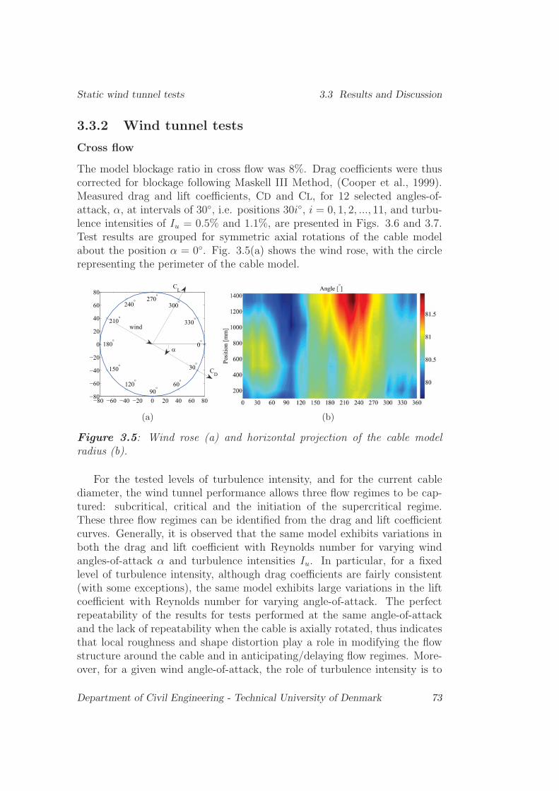
Static wind tunnel tests 3.3 Results and Discussion
3.3.2 Wind tunnel tests
Cross flow
The model blockage ratio in cross flow was 8%. Drag coefficients were thuscorrected for blockage following Maskell III Method, (Cooper et al., 1999).Measured drag and lift coefficients, CD and CL, for 12 selected angles-of-attack, α, at intervals of 30◦, i.e. positions 30i◦, i = 0, 1, 2, ..., 11, and turbu-lence intensities of Iu = 0.5% and 1.1%, are presented in Figs. 3.6 and 3.7.Test results are grouped for symmetric axial rotations of the cable modelabout the position α = 0◦. Fig. 3.5(a) shows the wind rose, with the circlerepresenting the perimeter of the cable model.
wind
CD
CL
wind
CD
CL
(a) (b)
Figure 3.5: Wind rose (a) and horizontal projection of the cable modelradius (b).
For the tested levels of turbulence intensity, and for the current cablediameter, the wind tunnel performance allows three flow regimes to be cap-tured: subcritical, critical and the initiation of the supercritical regime.These three flow regimes can be identified from the drag and lift coefficientcurves. Generally, it is observed that the same model exhibits variations inboth the drag and lift coefficient with Reynolds number for varying windangles-of-attack α and turbulence intensities Iu. In particular, for a fixedlevel of turbulence intensity, although drag coefficients are fairly consistent(with some exceptions), the same model exhibits large variations in the liftcoefficient with Reynolds number for varying angle-of-attack. The perfectrepeatability of the results for tests performed at the same angle-of-attackand the lack of repeatability when the cable is axially rotated, thus indicatesthat local roughness and shape distortion play a role in modifying the flowstructure around the cable and in anticipating/delaying flow regimes. More-over, for a given wind angle-of-attack, the role of turbulence intensity is to
Department of Civil Engineering - Technical University of Denmark 73

3.3 Results and Discussion Static wind tunnel tests
promote earlier flow transitions.
0.30.5 1 1.5 2 2.5 3 3.3x 10⁵
0.3
0.4
0.5
0.6
0.7
0.8
0.9
1
1.1
1.2
1.3
Reynolds number
Dra
g co
effic
ient
=0 (Iu=0.5%)
=0 (Iu=1.1%) (*)
=180 (Iu=0.5%)
=180 (Iu=1.1%)
(a)
0.30.5 1 1.5 2 2.5 3 3.3x 10⁵
0.3
0.4
0.5
0.6
0.7
0.8
0.9
1
1.1
1.2
1.3
Reynolds number
Dra
g co
effic
ient
=90 (Iu=0.5%)
=90 (Iu=1.1%)
=270 (Iu=0.5%)
=270 (Iu=1.1%)
(b)
0.30.5 1 1.5 2 2.5 3 3.3x 10⁵
0.3
0.4
0.5
0.6
0.7
0.8
0.9
1
1.1
1.2
1.3
Reynolds number
Dra
g co
effic
ient
=30 (Iu=0.5%)
=30 (Iu=1.1%)
=330 (Iu=0.5%)
=330 (Iu=1.1%)
(c)
0.30.5 1 1.5 2 2.5 3 3.3x 10⁵
0.3
0.4
0.5
0.6
0.7
0.8
0.9
1
1.1
1.2
1.3
Reynolds number
Dra
g co
effic
ient
=60 (Iu=0.5%)
=60 (Iu=1.1%)
=300 (Iu=0.5%)
=300 (Iu=1.1%)
(d)
0.30.5 1 1.5 2 2.5 3 3.3x 10⁵
0.3
0.4
0.5
0.6
0.7
0.8
0.9
1
1.1
1.2
1.3
Reynolds number
Dra
g co
effic
ient
=120 (Iu=0.5%)
=120 (Iu=1.1%)
=240 (Iu=0.5%)
=240 (Iu=1.1%)
(e)
0.30.5 1 1.5 2 2.5 3 3.3x 10⁵
0.3
0.4
0.5
0.6
0.7
0.8
0.9
1
1.1
1.2
1.3
Reynolds number
Dra
g co
effic
ient
=150 (Iu=0.5%)
=150 (Iu=1.1%)
=210 (Iu=0.5%)
=210 (Iu=1.1%)
(f)
Figure 3.6: Drag coefficients over the tested wind angles-of-attack α, Iu =0.5% and 1.1%. (∗) from (Kleissl and Georgakis, 2011)
For the lower turbulence intensity of Iu = 0.5%, the duration of the
74 Department of Civil Engineering - Technical University of Denmark

Static wind tunnel tests 3.3 Results and Discussion
0.30.5 1 1.5 2 2.5 3 3.3x 10⁵
00.2
11.2
Reynolds number
Lift
coef
ficie
nt
=0 (Iu=0.5%)
=0 (Iu=1.1%)
(Iu=0.5%)
(Iu=1.1%)
(a)
0.30.5 1 1.5 2 2.5 3 3.3x 10⁵
10.0.0.0.2
00.20.0.0.
11.2
Reynolds number
Lift
coef
ficie
nt
=90 (Iu=0.5%)
=90 (Iu=1.1%)
=270 (Iu=0.5%)
=270 (Iu=1.1%)
(b)
0.30.5 1 1.5 2 2.5 3 3.3x 10⁵
10.0.0.0.2
00.20.0.0.
11.2
Reynolds number
Lift
coef
ficie
nt
=30 (Iu=0.5%)
=30 (Iu=1.1%)
=330 (Iu=0.5%)
=330 (Iu=1.1%)
(c)
0.30.5 1 1.5 2 2.5 3 3.3x 10⁵
00.2
11.2
Reynolds number
Lift
coef
ficie
nt
(Iu=0.5%)
(Iu=1.1%)
=300 (Iu=0.5%)
=300 (Iu=1.1%)
(d)
0.30.5 1 1.5 2 2.5 3 3.3x 10⁵
10.0.0.0.2
00.20.0.0.
11.2
Reynolds number
Lift
coef
ficie
nt
=120 (Iu=0.5%)
=120 (Iu=1.1%)
=2 0 (Iu=0.5%)
=2 0 (Iu=1.1%)
(e)
0.30.5 1 1.5 2 2.5 3 3.3x 10⁵
00.2
11.2
Reynolds number
Lift
coef
ficie
nt
=150 (Iu=0.5%)
=150 (Iu=1.1%)
=210 (Iu=0.5%)
=210 (Iu=1.1%)
(f)
Figure 3.7: Lift coefficients over the tested wind angles-of-attack α, Iu =0.5% and 1.1%.
subcritical and critical regimes, is strongly dependent on the tested windangle-of-attack. In particular, the upper limit of the subcritical regime, i.e.
Department of Civil Engineering - Technical University of Denmark 75

3.3 Results and Discussion Static wind tunnel tests
the Reynolds number marking transition to critical, identified by the ap-pearance of a steady lift, and the simultaneous drop in the drag coefficient,ranges in the interval of Re = 1 − 2.7 × 10⁵. In contrast, the upper limitof the critical regime, made evident by the recovery of the drag coefficient,after the crisis, and the occurrence of a constant lift equal or close to zero,ranges in the interval of Re = 3 − 3.22 × 10⁵. Larger consistency in theupper, rather than in the lower limit of the critical Reynolds number regimefor varying angles-of-attack, implies that, for the test cases where the crit-ical regime is initiated earlier, the regime lasts for a broader total rangeof Reynolds number. This effect is particularly evident for the test casesα = 120◦ and α = 240◦, (see Figs.3.6(e) and 3.7(e)), where a large liftdevelops over a range of Re = 1.04 × 10⁵ − 3.21 × 10⁵ (α = 120◦), andRe = 1.06 × 10⁵ − 3.12 × 10⁵ (α = 240◦), and is accompanied by a con-tinuously dropping drag, significantly lower, through the whole critical Rerange, than for other tested angles-of-attack. It should be noted that forthese two test cases, an indented commercial label, distributed along thefull length of the HDPE tubing, which increases the surface roughness ofthe tubing locally, is placed at 60◦ clockwise (for α = 120◦) and 60◦ coun-terclockwise (for α = 240◦) from the flow stagnation line. The role of thelabeling roughness in triggering flow transitions is furthermore confirmed bythe observed opposite sign of the lift coefficient for the two tested angles-ofattack. Based on the development of the drag coefficient curves in Fig.3.6(e),it is assumed that the role of the indented labeling is similar to that of a trip-ping wire installed on the surface of a circular cylinder at a critical angularposition from the stagnation line, (Igaraschi, 1986a). Igaraschi (1986a) infact demonstrated that the boundary layer upstream of a tripping wire firstdecelerates, then separates, and finally forms an upstream separated region.A second separation takes place from the tripping wire itself, thus forminga downstream separated region. The downstream and upstream separatedregions represent two consecutive separation bubbles occurring on the sameside of the model which re-attach respectively at the tripping wire and atthe cable surface position. This flow structure leads to a significant decreaseof the drag coefficient when compared to the a smooth cable. Unfortunately,Igaraschi (1986a) did not present the lift coefficient. The smallest trippingwire size used by Igaraschi (1986a), which provoked this aerodynamic effectwas 0.4 mm thick, thus 4 times thicker than the maximum height (Ra) of thecommercial indentation. Although thinner than Igarashi’s tripping wire, thecommercial label must play a role in disturbing the flow around the cable,given the trend of the drag and the lift curves in Figs.3.6(e) and 3.7(e), i.e. asignificant decrease of the drag coefficient though the whole critical Re range,similar to that described by Igaraschi (1986a), accompanied by a large lift,
76 Department of Civil Engineering - Technical University of Denmark

Static wind tunnel tests 3.3 Results and Discussion
which doesn’t return to zero, after the end of the critical Re range. Finallyit should be noted that, since at low Reynolds numbers surface irregularitiesof a microscopic extent are normally completely embedded in the boundarylayer, the localized roughness begins to play a role in triggering flow separa-tion and reattachment only when its thickness overcomes the thickness of theboundary layer. The observed drag and lift tendencies in Figs. 3.6(e) and3.7(e) seem to suggest that the thickness of the label and the accompanyingflow structure produced by it overcome the thickness of the boundary layerat lower Reynolds number than for other tested wind angles-of-attack. Forthe other tested angles-of-attack, it is apparent that minor disturbances inthe cable’s shape and roughness trigger the generally observed narrow liftaccompanied by a typical steep crisis of the drag coefficient in the criticalrange. Given the non-perfect circularity of the cable model, symmetric flowconditions may never be achieved in the supercritical range. This is clearlyindicated by the non-zero lift, accompanied by a recovery of the drag coeffi-cient after the crisis.
At the increased turbulence intensity of Iu = 1.1%, a change is experi-enced in the magnitude of the drag and lift coefficients due to the general roleof the turbulence intensity in triggering earlier transitions in the flow regimes.The angle-of-attack dependency of the aerodynamic coefficients is still sig-nificant. It is interesting to observe that for α = 120◦ and α = 240◦, (seeFigs.3.6(e) and 3.7(e)), a large magnitude lift coefficient over a wider rangeof Reynolds number, accompanied by a continuously decreasing drag, stillpersists as found for the turbulence intensity of Iu = 0.5%. Moreover, due tothe increased turbulence intensity, the corresponding Reynolds number forthe development of the lift coefficient is lower. After the end of the criticalRe range, the lift doesn’t stabilize to zero due to the non-establishment ofsymmetric flow.
The mean drag and lift coefficients for the tested angles-of attack range,α = 0◦ − 330◦, and for the two levels of turbulence intensity, Iu = 0.5% and1.1%, are presented in Figs. 3.8.
The mean drag coefficient can more readily be used for design or theo-retical analysis purposes. On the other hand, the actual lift coefficient of thecable model is not well represented by its average through the tested angle-of-attack range. The mean lift coefficient is instead representative of thedistribution of surface disturbances over the cable model, and of how thesesurface disturbances are effective in changing the the aerodynamic behaviorof the cable model for varying angles-of-attack. For the two tested levels ofturbulence intensity, the mean lift coefficient is very close to zero for the fullrange of Reynolds numbers except in the critical region. It is unlikely thata mean zero lift could be expected throughout the full range of Reynolds
Department of Civil Engineering - Technical University of Denmark 77

3.3 Results and Discussion Static wind tunnel tests
0.30.5 1 1.5 2 2.5 3 3.3x 10⁵
0.3
0.4
0.5
0.6
0.7
0.8
0.9
1
1.1
1.2
1.3
Reynolds number
Mea
n dr
ag c
oeff
icie
nt
Iu = 0.5%Iu=1.1%
(a)
0.30.5 1 1.5 2 2.5 3 3.3x 10⁵
0.10.12
0.10.00.00.00.02
00.020.00.00.0
0.10.120.1
Reynolds number
Mea
n lif
t coe
ffic
ient
Iu = 0.5%Iu=1.1%
(b)
Figure 3.8: Mean drag coefficient (a) and mean lift coefficient (b) over thetested wind angles-of-attack α, Iu = 0.5% and 1.1%, Φ = 90◦.
numbers. Even in the ideal case of a perfectly symmetrical cable model, freefrom disturbances on its surface, a zero averaged lift coefficient isn’t likelyto occur due to the establishment of the bi-stable flow, i.e. the random for-mation of the first separation bubble on either side of the cable and thus thelack of repeatability of the sign of the lift coefficient. On the other hand, ifthe cable model is characterized by a surface disturbance, like a microscopicprotuberance, located on only one side of its surface and at a certain angularposition from the stagnation line, the first separation bubble will occur oneither side of the cable’s surface, in such a way that the disturbance willlie in the critical area of the cable. The resulting lift coefficients will be ofopposite signs and the resulting average will be zero, given the assumptionthat the positive and negative magnitude of the experienced lifts are equal inabsolute value. On the other hand, when the axial rotation is such that theprotuberance is located out of the critical area, random bi-stable flow willoccur. Thus the total average lift will not be zero. Finally, for an actual cablewith an non-uniform distribution of surface roughness the average behavioris more complicated, and no prediction can be made.
Inclined cable
The wind-tunnel blockage was lower than 2% in all of the inclined cabletests. Therefore, no correction was performed for blockage. The drag andlift coefficient components, normal to cable axis, for varying relative cable-wind angles Φ, are presented in Fig. 3.9.
The drag and lift coefficient components are determined based on themean the free stream velocity component U. In the subcritical Reynolds
78 Department of Civil Engineering - Technical University of Denmark

Static wind tunnel tests 3.3 Results and Discussion
0.30.5 1 1.5 2 2.5 3 3.3x 10⁵
0.2
0.3
0.4
0.5
0.6
0.7
0.8
0.9
1
1.1
1.2
Reynolds number
Dra
g co
effic
ient
com
pone
nt n
orm
al to
cab
le
=90=75=70=65=60=55=50=45=40
(a)
0.30.5 1 1.5 2 2.5 3 3.3x 10⁵
0.0.0.0.50.0.30.20.1
00.10.20.30.
Reynolds number
Lift
coef
ficie
nt c
ompo
nent
nor
mal
to c
able
=90= 5= 0= 5= 0=55=50= 5= 0
(b)
Figure 3.9: Drag coefficient component normal to cable axis (a) and liftcoefficient component normal to cable axis (b) for varying relative cable-windangles Φ, Iu = 0.5%.
number range, the drag coefficient components normal to cable axis are gen-erally increasing, as the relative cable-wind angle Φ increases. Contrary tothis, the lift coefficient components normal to cable axis are generally closeto zero. The initiation of the critical Reynolds number range, made evidentby a drop in the drag coefficient component accompanied by the appearanceof a lift coefficient component, occurs as expected, as the relative cable-windangle Φ decreases. For Φ = 40◦, 45◦, and 50◦, the slope of the drag coefficientcomponent normal to cable-axis during the crisis is lower than for other testcases. Moreover, the lift coefficient component normal to cable axis is closerto zero in comparison to the other tested Φ angles throughout all the investi-gated Reynolds number ranges. When comparing the aerodynamic behaviorof the remaining relative cable-wind angles, i.e. Φ = 55◦−75◦, it is apparentthat the highest slope in the drag coefficient component is experienced forΦ = 65◦ − 75◦. Additionally for these angles, the critical Re range, fromRe ≈ 2−3×10⁵, is characterized by the appearance of a large lift coefficientcomponent. Relative cable-wind angle Φ = 60◦ is characterized by a lift co-efficient component normal to cable axis occurring over a much wider rangeof Reynolds numbers, accompanied by a slightly lower slope of for the dragcoefficient component normal to cable axis in the critical Re region.
Larose et al. (2005) conducted wind-tunnel tests on a full scale yawed ca-ble model, whose ends where fitted with half spheres. Tests were performedfor the same total range of Reynolds number as the present tests, but at anincreased turbulence intensity level, Iu = 2.5%. Even if a direct comparisonwith the present results can not be established due to different test condi-tions, it is generally observed that the magnitude and the features of the drag
Department of Civil Engineering - Technical University of Denmark 79

3.3 Results and Discussion Static wind tunnel tests
and lift coefficient component curves are similar between the two test cam-paigns. In particular, the general tendency of drag component to increasewith increasing relative cable-wind angle Φ and the non-zero lift through thefull tested range of Reynolds number can be observed.
Based on dynamic and static tests undertaken on full-scale and scaledmodels respectively, Cheng et al. (2008a) predicted that a cable declining inthe wind direction, and characterized by a relative cable-wind angle Θ = 60◦,may undergo divergent-type motion. It is for this reason that detailed windangle-of-attack and Reynolds number sweeps have been performed for thisangle. Figs. 3.10 and 3.11 show the measured drag and lift coefficient
0.30.5 1 1.5 2 2.5 3 3.3x 10⁵
0.2
0.3
0.4
0.5
0.6
0.7
0.8
0.9
1
Reynolds number
Dra
g co
effic
ient
com
pone
nt n
orm
al to
cab
le
=30=330=60=300
(a)
0.30.5 1 1.5 2 2.5 3 3.3x 10⁵
0.2
0.3
0.4
0.5
0.6
0.7
0.8
0.9
1
Reynolds number
Dra
g co
effic
ient
com
pone
nt n
orm
al to
cab
le
=120=240=150=210
(b)
0.30.5 1 1.5 2 2.5 3 3.3x 10⁵
0.2
0.3
0.4
0.5
0.6
0.7
0.8
0.9
1
Reynolds number
Dra
g co
effic
ient
com
pone
nt n
orm
al to
cab
le
=0=180=90=270
(c)
Figure 3.10: Drag coefficient component normal to cable axis for varyingwind angles-of-attack α, Φ = 60◦ and Iu = 0.5% .
components normal to cable axis for Φ = 60◦ and varying wind angles-of-attack, for a turbulence intensity Iu = 0.5%. As experienced for the cross-flow case, the drag coefficient component normal to cable axis remains fairlyconsistent, while the lift coefficient component normal to cable axis exhibits
80 Department of Civil Engineering - Technical University of Denmark

Static wind tunnel tests 3.3 Results and Discussion
0.30.5 1 1.5 2 2.5 3 3.3x 10⁵
0.5
0.
0.3
0.2
0.1
0
0.1
0.2
0.3
0.
0.5
Reynolds number
Lift
coef
ficie
nt c
ompo
nent
nor
mal
to c
able
=30=330=60=300
(a)
0.30.5 1 1.5 2 2.5 3 3.3x 10⁵
0.5
0.
0.3
0.2
0.1
0
0.1
0.2
0.3
0.
0.5
Reynolds number
Lift
coef
ficie
nt c
ompo
nene
t nor
mal
to c
able
=120=2 0=150=210
(b)
0.30.5 1 1.5 2 2.5 3 3.3x 10⁵
0.5
0.
0.3
0.2
0.1
0
0.1
0.2
0.3
0.
0.5
Reynolds number
Lift
coef
ficie
nt c
ompo
nent
nor
mal
to c
able
=0=180=90=270
(c)
Figure 3.11: Lift coefficient component normal to cable axis for varyingwind angles-of-attack α, Φ = 60◦ and Iu = 0.5% .
large variations as the wind angle-of attack is changed. For Reynolds numberin the range of Re ≈ 1.5 − 2 × 10⁵, the drag coefficient components are inthe critical Reynolds range, for all tested angle-of-attack. The crisis here isquite abrupt, i.e. the negative slope of the drag component curve is quitelarge in absolute value. This implies that the significant decrease in the dragcoefficient component from the subcritical value of approximately 0.9 to theend-of-critical-range value of approximately 0.3, could occur within a smallregion of Reynolds numbers. The decrease in the drag coefficient componentwas accompanied by a non-zero lift. In particular as the angle-of-attackchanges, large variations of the measured lift coefficient component with thewind angle-of-attack occur, either in sign or in amplitude.
The mean drag and lift coefficient component normal to cable axis overthe full tested range of angle-of-attack, α = 0◦ − 330◦, for a turbulenceintensity Iu = 0.5%, are shown in Fig. 3.12. Again, while the drag coefficient
Department of Civil Engineering - Technical University of Denmark 81

3.3 Results and Discussion Static wind tunnel tests
component could be used for design or theoretical analysis, the mean liftcoefficient component is only a representation of the average effect of surfaceirregularities on the cable’s aerodynamic response.
0.30.5 1 1.5 2 2.5 3 3.3x 10⁵
0.2
0.3
0.4
0.5
0.6
0.7
0.8
0.9
1
Reynolds number, Re Mea
n dr
ag c
oeff
icie
nt c
ompo
nent
nor
mal
to c
able
(a)
0.30.5 1 1.5 2 2.5 3 3.3x 10⁵
0.10.120.1
0.00.00.00.02
00.020.00.00.00.1
0.120.1
Reynolds number, Re Mea
n lif
t coe
ffic
ient
com
pone
nt n
orm
al to
cab
le
(b)
Figure 3.12: Mean drag coefficient component (a) and mean lift coefficientcomponent (b) normal to cable axis over the tested wind angles-of-attack α,Φ = 60◦ and Iu = 0.5%.
Force correlation and repeatability
The averaged drag and lift forces measured at each cable end were usedto determine the cable’s drag and lift coefficients. In cross-flow and in thesubcritical range, the measured drag and lift forces at either ends of the cablegenerally follow each other, with a maximum deviation of approximately 1%for the tested range of wind angles-of-attack α. More significant deviationsare observed in the critical Reynolds number range where the cable end forcesdiffer up to 10%. For the inclined/yawed test cases, the drag and lift forcecomponents again follow each other, with deviations though in the order of10 − 15% in the critical Reynolds number range. These deviations extendin certain cases into the subcritical range for the lift force. It is conjecturedthat variations in the measured aerodynamic forces along the model are dueto the non-uniform distribution of surface disturbances, which trigger, in thecritical Reynolds number range, a variation in the spacial structure of theflow along the cable. The three dimensional character of the flow structurearound inclined cables, has also been reported by Larose et al. (2003) and hasbeen considered responsible, together with critical Reynolds number effects,for potential aerodynamic instabilities.
Test repeatability has been checked by performing each test, i.e. Reynoldsnumber sweeps for a selected relative cable-wind angle Φ and wind angle-of-
82 Department of Civil Engineering - Technical University of Denmark

Static wind tunnel tests 3.4 Conclusion
attack α, at least twice in one day. In Figs. 3.6-3.7, 3.9, 3.10-3.11, datapoints from the first and second test repetition performed in the same dayare reported for each test case. As can be observed, the degree of datarepeatability is very high. A check on the repeatability was performed byrepeating Reynolds number sweeps, for selected relative cable-wind anglesand wind angles-of-attack, several days after the first tests. The same degreeof data repeatability could be obtained.
3.4 Conclusion
Bridge cable force coefficients based on wind tunnel tests should not neces-sarily be regarded as invariant with wind angle-of-attack. Static wind tunneltests conducted in cross and inclined flow for a short bridge cable model,characterized by a non-uniform distribution of surface roughness and shape,demonstrate that significant variations in the aerodynamic coefficients canbe observed for varying wind angles-of-attack. These changes in the aero-dynamic coefficients can be triggered by small geometrical imperfections ofthe cable model, such as surface roughness alterations or distortions of theshape. Assuming the validity of the quasi-steady theory, negative aerody-namic damping can be predicted in the critical Reynolds number range wherethe drag coefficient is reduced to its minimum and the lift coefficient experi-ences significant oscillations in sign and amplitude with angle-of-attack.
Note that, although important for theoretical modeling and section modeltesting, variations in the drag and lift coefficients with wind angle-of-attackmay not ultimately be important when averaged over the full length of aninclined structural cable.
Department of Civil Engineering - Technical University of Denmark 83

3.4 Conclusion Static wind tunnel tests
84 Department of Civil Engineering - Technical University of Denmark

Bibliography
Cheng, S., Larose G.L., Savage, M., Tanaka, H., Irwin, P., 2008a. Experi-mental study on the wind-induced vibration of a dry inclined cable - PartI: Phenomena. J. Wind Eng. Ind. Aerodyn. 96 (12), 2231-2253.
Cooper, K., Mercker, E., Wiedemann, J., 1999. Improved blockage correc-tions for bluff-bodies in closed and open wind tunnels. In: 10th Interna-tional Conference Wind Engineering, Copenhagen, pp. 1627-1634.
Fage, A., Warsap, G.H., 1929. The effects of turbulence and surface roughnesson the drag of a circular cylinder. Brit. Aero. Res. Council, 1283.
Flamand, O., 1995. Rain-wind induced vibrations of cables. J. Wind Eng.Ind. Aerodyn. 57 (2/3), 353-362.
Flamand, O., Boujard, O., 2009. A comparison between dry cylinder gal-loping and rain-wind induced excitation. In: 5th European and Africanconference on wind engineering, Florence, pp. 485-488.
Georgakis, C.T., Koss, H.H., Ricciardelli, F., 2009. Design specifications fora novel climatic wind tunnel for testing of structural cables. In: 8th Inter-national Symposium on Cable Dynamics, Paris, pp. 333-340.
Igarashi, T., 1986a. Effect of tripping wires on the flow around a circularcylinder normal to an airstream. Bull. JSME 28, 2917-2924.
Kamiya, N., Suzuki, S., Nishi, T., 1979. On the aerodynamic force actingon a circular cylinder in the critical range of Reynolds number. In: AIAAmeeting, paper79-1975.
Kleissl, K., Georgakis, C.T., 2011. Preliminary comparison of static windtunnel tests of bridge cables with helical fillets and a pattern-indentedsurface. In: 13th International Wind Engineering Conference, Amsterdam.
85

BIBLIOGRAPHY BIBLIOGRAPHY
Larose, G.L., Jakobsen, J.B., Savage, M.G., 2003. Wind-tunnel experi-ments on an inclined and yawed stay cable model in the critical Reynoldsnumber range. In: 5th International Symposium Cable Dynamics, SantaMargherita Ligure, pp. 279-286.
Larose, G.L., Zasso, A., Giappino, S., 2005. Experiments on a yawed staycable in turbulent flow in the critical Reynolds number range. In: 6thInternational Symposium Cable Dynamics, Charleston, pp. 279-286.
Macdonald, J.HJ., Larose G.L., 2008a. Two-degree-of-freedom inclined gal-loping - Part 1: general formulation and solution for perfectly tuned sys-tem. J. Wind Eng. Ind. Aerodyn. 96 (3), 291-307.
Macdonald, J.HJ., Private communication. University of Bristol, U.K.
Matsumoto, M., Yagi, T., Hatsuda, H., Shima, T., Tanaka, M., 2010. Drygalloping characteristics and its mechanism for yawed/inclined cylinders.J. Wind Eng. Ind. Aerodyn. 98 (6/7), 317-327.
Matteoni, G., Georgakis, C.T., 2011. Effects of bridge cable surface roughnessand cross-sectional distortion on aerodynamic force coefficients. In: 13thInternational Wind Engineering Conference, Amsterdam.
Matteoni, G., Georgakis, C.T., 2011. Aerodynamic coefficients of dry in-clined cables in smooth flow. In: 9th International Symposium on CableDynamics, Shanghai, pp. 365-372.
Niemann, H.-J., Holscher, N., 1990. A review of recent experiments on theflow past circular cylinders. J. Wind Eng. Ind. Aerodyn. 33 (1/2), 197-209.
Schewe, G., 1983. On the force fluctuations acting on a circular cylinder incrossflow from subcritical up to transcritical Reynolds numbers. J. FluidMech. 133, 265-285.
Schewe, G., 1986. Sensitivity of transition phenomena to small perturbationsin the flow field round a circular cylinder. J. Fluid Mech. 172, 33-46.
Zdravkovich, M.M., 1997. Flow around circular cylinders, vol.1: Fundamen-tals. Oxford University Press, New York.
Zdravkovich, M.M., 2003. Flow around circular cylinders, vol.2: Applica-tions. Oxford University Press, New York.
86 Department of Civil Engineering - Technical University of Denmark

Chapter 4
Passive-dynamic wind tunneltests in dry state
The results presented in this chapter are taken from the paper Effects ofsurface roughness and cross-sectional distortion on the wind-induced responseof bridge cables in dry conditions, G. Matteoni, C.T. Georgakis, submittedto the Journal of Wind Engineering and Industrial Aerodynamics.
Abstract
Theoretical and experimental investigations to date have assumed that bridgestay cables can be modelled as ideal circular cylinders and that their aero-dynamic coefficients are invariant with wind angle-of-attack. On the otherhand it has been demonstrated that bridge cables are characterised by localalterations of their inherent surface roughness and shape. Small deviationsfrom ideal circularity result in significant changes in the static drag and liftcoefficients with Reynolds number. The present study focuses on the wind-induced response of a full-scale yawed bridge cable section model, for vary-ing Reynolds numbers and wind angles-of-attack. Based on passive-dynamicwind tunnel tests, it is shown that the in-plane aerodynamic damping of abridge cable section, and the overall dynamic response, are strongly affectedby changes in the wind angle-of-attack. Using the drag and and lift coeffi-cients, determined in static conditions for an identical cable model as the oneused for passive-dynamic tests, the in-plane aerodynamic damping is evalu-ated by employing a one-degree-of-freedom (1 DOF) quasi-steady analyticalmodel. Similarly, it is shown that regions of instability associated with theoccurrence of negative aerodynamic damping, are strongly dependent on thewind angle-of-attack.
87

4.1 Introduction Passive-dynamic wind tunnel tests in dry state
4.1 Introduction
4.1.1 Overview of the dry inclined cable instability
The vibration of dry inclined cables, i.e. in the absence of rain or ice ac-cretions, was first described by Japanese researchers. It is characterised bythe presence of divergent-type vibrations, i.e. dry inclined galloping, or bylimited amplitude vibrations, i.e. so called vortex shedding at high reducedvelocities.
The cause of dry vibration is attributed by most authors to effects asso-ciated with the critical Reynolds number. In this range, small imperfectionsin the cable geometry, such as the ovalisation of the HDPE tube covering thecables, or added surface roughness are sufficient to introduce important flowtransitions, which can lead to cable vibrations, particularly if the inherentstructural damping of the cable is very low, (Larose and Zan, 2001). More-over, for the specific case of dry inclined galloping, the secondary axial flowis considered to play a role. It is hypothesized that it acts as an air cur-tain, interrupting the fluid interaction between the cable’s separated shearlayers and generating an unsteady inner circulatory flow at either the lowerleeward or upper leeward side of the cable circular surface. This determinesa region of significantly lower surface pressure which results in higher oscil-latory aerodynamic forces and consequently violent vibrations, (Matsumotoet al., 1990). On the other hand, the cause of high speed vortex shedding isattributed to the interaction between the conventional Karman vortex shed-ding and the axial vortex shedding, with the frequency of the latter beingone third of the former. This implies that the cylinder’s response is amplifiedwhen the axial vortexes shed once every three Karman vortices from eitherside of the cable’s model, (Matsumoto et al., 1999).
Vibration of dry inclined cables has never been fully verified full-scale,and only a limited number of reports exist, for example (Virlogeux, 1998),(Irwin et al., 1999), (Boujard, 2007), (Zuo and Jones, 2010), (Matsumotoet al., 2010). On the other hand, it has been reproduced in wind tunnelexperiments. By comparing results from different experimental campaigns,it is apparent that the characteristics of dry instability, are strongly affectedby the test conditions.
The first experimental investigation on the instability of inclined/yawedfull-scale bridge cables in dry conditions was undertaken by Saito et al.(1994). Based on dynamic wind tunnel tests performed on a cable modelidentical in mass as an actual bridge cable from the Higashi-Kobe Bridge inJapan, Saito et al. (1994) derived an instability criterion which suggests thatdry inclined cable vibration can be excited at very low wind velocities cor-
88 Department of Civil Engineering - Technical University of Denmark

Passive-dynamic wind tunnel tests in dry state 4.1 Introduction
responding to the subcritical Reynolds number range. The excitation can’tbe suppressed even if the cable’s Scrouton number or structural damping issignificantly increased. The former is defined herewith as
Sc =mζ
ρD2(4.1)
where ζ is the cable’s structural damping ratio, m is the cable’s mass perunit length, ρ is the air density and D is the cable’s diameter. This impliedthat the majority of bridge cables of exisiting bridges might be prone todry inclined instability. A second instability criterion for dry cable vibrationwas later derived by Honda et al. (1995). The criterion suggests that forwind velocities corresponding to the transition from the subcritical to thecritical Reynolds number regime divergent motion starts. Experimental testsundertaken by Miyata et al. (1994b) confirmed this finding. Honda et al.(1995) also observed that a significant increase in the structural damping(and thus in the Scrouton number) is not sufficient to suppress the instability.
Some years later, a series of wind tunnel tests were undertaken in collab-oration between the University of Ottawa, Rowan Williams Davies and Irwin(RWDI), and the National Research Council Canada. The experimental cam-paign was part of a large study commissioned by the US Federal HighwayAdministration (FHWA). The main objective of the study was to verify theexistence of dry inclined galloping and validate the severe instability crite-rion proposed by Saito et al. (1994). The test campaign consisted of threephases. In the first phase it was observed, based on passive-dynamic windtunnel tests, that dry inclined cables can undergo two types of instability,i.e. a limited amplitude type, occurring over a narrow interval of wind veloc-ities within the critical Reynolds number range, i.e. vortex shedding at highreduced velocity, and a divergent type, which is generated for all wind ve-locities above the critical one in the critical Reynolds number range, i.e. dryinclined galloping, (Cheng et al., 2008a). Contrary to previous tests, the dryinclined galloping instability could be restricted by increasing the structuraldamping (or Scrouton number). Static wind tunnel tests undertaken in thesecond phase of the campaign served to clarify the origins of the dry inclinedgalloping instability. This was explained in a similar way as the conventionalgalloping of ice coated cables, i.e. in terms of the Den Hartog criterion,(Cheng et al., 2008b). As a result of the experimental tests undertaken dur-ing phase 1 and 2, the FHWA proposed a new stability criterion for dry cablevibration, (FHWA/HNTB, 2005). The criterion established a value of 10 asthe minimum desired Scrouton number for regular cable arrangements. Thecriterion is less conservative than the one established by Saito et al. (1994)and is currently used by bridge designers. In the third phase, displacement
Department of Civil Engineering - Technical University of Denmark 89

4.1 Introduction Passive-dynamic wind tunnel tests in dry state
and pressure measurements were performed on a cable section with identicalcharacteristics as the one used in phase 1, (Jacobsen et al., 2012). Divergentresponse was observed for a limited range of Reynolds numbers correspond-ing to the end of the critical region, where the drag coefficient drops to aminimum and a steady lift appears. This is in contrast with conventionalgalloping which occurs at any wind speed above the critical one. It wasfurther observed that, due to the effect of minor imperfections of the cablesurface or slight lack of roundness, the lift coefficient is a function of the cableorientation about its axis. Slight increases in the surface roughness of themodel, due to the localised accumulation of insects on the cable section, sig-nificantly affected the response of the cable. In connection with these latterfindings, a recent investigation undertaken by Matteoni and Georgakis (2012)showed that bridge cables are characterised by a non-uniform distribution ofsurface roughness and shape. Based on static wind tunnel tests undertakenon full-scale bridge cable section models, it was demonstrated that the dragand lift coefficient of both cross-flow and inclined/yawed bridge cable modelsare strongly dependent on the degree of axial rotation of the cable model,i.e. on the wind angle-of-attack. Some of the findings were also achieved byFlamand and Boujard (2009). Assuming quasi-steady theory, Matteoni andGeorgakis (2012) hypothesized that negative aerodynamic damping can bepredicted, especially in the critical Reynolds number range, where the dragcoefficient is reduced to its minimum, while the lift coefficient experiencessignificant variations with wind angle-of-attack. Nevertheless, no experimen-tal evidence of this occurrence, based on passive-dynamic tests, has been yetdemonstrated.
4.1.2 Objectives and findings of the present investiga-tion
Further to the work of Matteoni and Georgakis (2012), the current work in-vestigates the effects of surface roughness and cross-sectional distortion onthe wind-induced response of bridge cables in dry conditions. In order tounderstand this dependency, passive-dynamic wind tunnel tests were under-taken on a section of a bridge cable inclined/yawed to the incoming wind. Thein-plane aerodynamic damping and the peak-to-peak amplitude of the cableresponse were identified for varying Reynolds numbers and varying degreesof axial rotation of the HDPE tubing, i.e. for varying wind angles-of-attack.Experimental observations of the investigation lead to the conclusion that dryinstability of inclined/yawed bridge cables is very sensitive to microscopic ge-ometrical imperfections of the cable model. It was found that the in-plane
90 Department of Civil Engineering - Technical University of Denmark

Passive-dynamic wind tunnel tests in dry state 4.2 Materials and Methods
aerodynamic damping, as well as the peak to peak amplitude, changed signif-icantly with Reynolds number for varying wind angles-of-attack. The uniquealteration in the test setup when the cable is axially rotated, i.e. the surfaceroughness and shape of the model exposed to the oncoming wind, was suffi-cient enough to significantly alter the wind-induced response, and to triggerthe cable instability over a broad range of Reynolds number.
The in-plane aerodynamic damping was additionally evaluated based onthe static drag and lift coefficients obtained by Matteoni and Georgakis(2012) for a cable model oriented at the same cable-wind angle Φ as inthe passive dynamic tests, for varying Reynolds numbers and wind angles-of-attack. This was done to compare the regions of dry instability basedon the passive-dynamic and static tests. For this, a one-degree-of-freedomquasi-steady analytical model developed by Macdonald and Larose (2006)was implemented. It is not directly possible to compare the regions of insta-bility based on the static and passive-dynamic tests. It should be noted that,due to a difference in the end conditions and in the relative roughness/shapedistribution in the critical area of the cable, i.e. where flow separation isexpected to occur, the flow regimes experienced by the static and passive-dynamic cable might not perfectly coincide. Nevertheless, both approachesdemonstrate that the aerodynamic damping is strongly dependent on thewind angle-of-attack.
4.2 Materials and Methods
4.2.1 Passive-dynamic wind tunnel tests
Passive-dynamic tunnel tests were performed at the new DTU/Force Cli-matic Wind Tunnel in Lyngby. The wind tunnel is a close circuit with a testsection size of L×W ×H = 5 m ×2 m ×2 m. Technical spefications of thewind tunnel are reported by Georgakis et al. (2009).
The tested cable section model was made of a plain HDPE tube, pro-vided by bridge cable suppliers, with a nominal diameter of 160 mm, placedon an inner aluminum tube, for increased rigidity. The tubing, of the sametype as the one used for static wind tunnel tests undertaken by Matteoniand Georgakis (2012), was not characterised by a uniform roughness, duethe presence of minor scratches and a 4 mm wide commercial indentationdistributed all along its length, see Fig. 4.1. The roughness average, mea-sured both in the direction of extrusion and of the wind flow, was found tobe in the range of 0.7-2 μm. Increased roughness average was found alongthe commercial indentation, i.e. in the range of 50-100 μm. The measured
Department of Civil Engineering - Technical University of Denmark 91

4.2 Materials and Methods Passive-dynamic wind tunnel tests in dry state
roughness average of the tubing was comparable to values measured on thefull-scale in-situ cables of the Øresund Bridge. Roundness measurements ofthe cable model, i.e. including the inner aluminum tube, showed that it isnearly circular, with a maximum deviation of the local diameter of 1.25 %(1mm) from its nominal value, (Matteoni and Georgakis, 2012).
Figure 4.1: HDPE tubing used for passive-dynamic wind tunnel tests.
The dynamic rig consisted of two hollow square steel sections positionedabove and underneath the steel frame of the wind tunnel test chamber. Thecable model was supported elastically on the outside of the wind tunnel testsection, whilst protruding across lateral openings of 300 × 730 mm2 area.Circular hollow pipes were mounted to the hollow square structural sectionsusing special light weight steel fittings, and served to support the springs.Fig. 5.2.2 shows the cable model seen from the inside of the wind tunnel testsection.
Figure 4.2: Cable model seen from the inside of the wind tunnel test cham-ber.
Extension coil springs, produced by Lesjofors, were used as elastic sup-ports. Their sizes were determined in terms of number of coils, outer diameter
92 Department of Civil Engineering - Technical University of Denmark

Passive-dynamic wind tunnel tests in dry state 4.2 Materials and Methods
and wire diameter in order to achieve the desired frequency. Four extensioncoil springs, two per each cable end were used to allow vibration of the cablemodel in the in-plane direction. These were oriented perpendicularly to thecable axis, and belonged to the plane containing the cable axis and its pro-jection in the horizontal plane. The size of the upper springs (i.e. in terms
(a)
(b)
Figure 4.3: Cable model upper end (a) and lower end (b).
of outer diameter and wire diameters) was larger than the lower springs, asthe upper springs are supposed to carry the weight of the cable model. Thecombined spring constant for the in-plane springs is c = 844.3 N/m. Fig. 4.3shows a detail of the cable upper and lower end with in-plane springs. An ax-ial spring wire was connected to the upper end of the cable model and servedto carry the component of the gravitational force in the axial direction. The
Department of Civil Engineering - Technical University of Denmark 93

4.2 Materials and Methods Passive-dynamic wind tunnel tests in dry state
out-of-plane motion was prevented by use of four wires, two per each cableend, placed in the plane perdicular to the one which contains the in-planesprings (see Fig. 5.3). Additional technical specifications on the dynamic rigare reported by Eriksen (2012).
In Fig. 5.3 the cable’s geometrical attitude in the wind tunnel testschamber is identified. (X, Y, Z) is a global cartesian reference system, withY parallel to the along-wind velocity U , and Z being vertical. (x, y, z) is thecable local reference system, with z being parallel to the cable’s longitudinalaxis, ad xy belonging to the cross-sectional plane perpendicular to the z axis.The cable’s geometrical attitude is identified by the relative cable wind angleΦ, i.e. the angle between the wind direction and the cable axis, obtainedby combining the vertical inclination, Θ, and the horizontal yaw, β. In thepresent tests, the cable was installed declining in the wind direction witha vertical inclination of Θ = 25◦, and a horizontal yaw of β = 60◦. Theresulting cable-wind angle, i.e. Φ = 63◦, is in the range where dry inclnedgalloping is predicted to occur (Raaesi et al., 2013). The wind angle-of-attack, α, identifies the degree of axial rotation of the cable, i.e. the angleformed by the projection of the free stream velocity U in the xy plane, UN ,(normal wind velocity) and the y axis, so that
UN = U
√sin2 β + sin2 Θcos2 β (4.2)
Tests were performed for ten selected wind angles-of-attack, namely α = 0◦,30◦, 60◦, 90◦, 105◦, 120◦, 150◦, 180◦, 195◦, 210◦, i.e. at intervals of Δα =15◦-30◦. Effects of any flow disturbance on the cable surface could thus beinvestigated. This could be done by assuming that disturbances positionedabove and below the flow stagnation line produce the same effect on theaerodynamic behaviour.
The total length of the cable model was Ltot = 3.35 m. The effectivelength, i.e. the length of the model inside of the wind tunnel test chamber,was Leff = 2.55 m. The total mass of the cable model was mtot = 46.09 kg,while the effective mass per unit length of the model, i.e. obtained consideringits total length, was meff = 18.07 kg/m. Note that the mass per unit lengthof full-scale proto-type bridge cables can vary in the range 40 − 120 kg/m.Thus the mass scaling factor between the current and prototype bridge cablesranges between 1:2.21 and 1:6.64. The cable’s structural frequency was 1.10Hz, while the measured structural damping, determined as the rig dampingat zero wind velocity, was 0.1%. Based on this, the cable’s Scrouton numberwas equal to 0.56.
All tests were conducted for a range of wind velocites of 0-30 m/s, insmooth flow conditions, i.e. for a uniform along cable axis turbulence inten-
94 Department of Civil Engineering - Technical University of Denmark

Passive-dynamic wind tunnel tests in dry state 4.2 Materials and Methods
Figure 4.4: Illustration of dynamic rig geometry.
sity of Iu = 0.53%, measured by use of a cobra probe at velocities of 9.6, 12.6and 15.8 m/s.
Table 5.1 summarises the test parameters for the cable model.
Cable diameter, D [m] 0.16Frequency of in-plane motion, f [Hz] 1.10
Vertical inclination, Θ [◦] 25Horizontal yaw, β [◦] 30Total length, Ltot [m] 3.35
Effective length, Leff [m] 2.55Total mass, mtot [kg] 46.09
Effective mass per unit length, meff [kg/m] 18.07Structural damping, ζs [%] 0.10Scrouton number, Sc [-] 0.56
Along-axis turbulence intensity, Iu [%] 0.53
Table 4.1: Test parameters for the cable model.
The model response in both in-plane and out-of-plane directions weremeasured by means of analogue laser displacement transducers producedby Waycon. The laser distance measurement is based on the triangulationprinciple. The laser transducers were fixed to the rig structure with the laserspot directed perpendicular to wooden plates mounted to the cable ends(see Figs. 4.3). The in-plane displacements were measured using a LAS-T-500 type laser, characterised by a range of 100-500 mm and a resolution of
Department of Civil Engineering - Technical University of Denmark 95
4.2 Materials and Methods Passive-dynamic wind tunnel tests in dry state
0.03-0.6 mm, while the (restricted) out-of-plane displacements were measuredusing a LAS-T-250 type laser, characterised by a range of 50-300 mm and aresolution of 0.02-0.35 mm. The average signal at the two cable ends, givingthe model displacement at mid length, was filtered in the time domain witha digital band-pass Butterworth filter in order to isolate the contribution ofthe in-plane vibration response.
In all tests the aerodynamic damping and the peak to peak amplitudeof the response were evaluated, by either letting the cable freely vibrateunder the wind or by manually exciting the cable. In particular, for windvelocities where the cable vibration grew spontaneously, the total dampingwas evaluated from the slope of the vibration growth. For the remainingwind velocities the total damping was evaluated by exciting the cable modelmanually, so as to reach an amplitude of vibration of approximately 1D-1.5D. The vibration decay indicated that the total damping was positive,thus the aerodynamic damping was either positive or negative but smallerin absolute value than the structural damping. The aerodynamic dampingwas evaluted as the difference between the total and the structural damping.For each tested wind velocity the mean and standard deviation aerodynamicdamping was evaluated based on a number of test repetitions, i.e. vibra-tion growth/decay events, comprising between 2 and 10. Finally, in orderto evaluate the dependency of the aerodynamic damping on the vibrationamplitude, the free decay/growth signals were divided into amplitude subin-tervals and the aerodynamic damping was evaluated for each of those. Fig.4.5 shows an example of the evaluation of the total aerodynamic dampingbased on the slope of a free decay response at 9 m/s for α = 210◦. Thetotal damping was evaluated for different ranges of vibration amplitude, i.e.1D-0.1D, 1D-0.75D, 0.75D-0.50D, 0.50D-0.25D, 0.25D-0.10D.
4.2.2 Static wind tunnel tests
Drag and lift coefficients determined from static wind tunnel tests performedon a full-scale inclined/yawed cable model (Matteoni and Georgakis, 2012),were implemented in the 1 DOF quasi-steady instability model developedby Macdonald and Larose (2006) in order to compare the regions instabilityobtained with the passive-dynamic tests. The static wind tunnel tests wereperformed for a shorter cable section model, made of a plain HDPE tubefixed to an inner aluminum tube. The HDPE tube was of the same type andprovided by the same suppliers as the tube used for passive dynamic tests.The static model, in contrast to the cable section used for passive-dynamictests, was tested with circular end plates and was completely installed onthe inside of the wind tunnel test chamber, see Fig. 4.6. The cable model
96 Department of Civil Engineering - Technical University of Denmark

Passive-dynamic wind tunnel tests in dry state 4.2 Materials and Methods
Figure 4.5: Example of evaluation of the total aerodynamic damping ζtotfor varying vibration amplitude intervals.
was installed at a relative cable-wind angle Φ = 60◦ obtained by combining avertical inclination of Θ = 55◦ and a horizontal yaw of β = 30◦. Aerodynamicforces at the cable ends were measured by use of 6 DOF force transducers.A 3◦ descrepancy exists between the cable-wind angle used in the static andpassive-dynamic tests. This is due to space constrictions in the dynamic testset-up which didn’t allow for the same relative cable-wind angle as in thestatic tests. Technical details on the experimental setup for the static testsare reported by Matteoni and Georgakis (2012).
Figure 4.6: Inclined test configuration in static conditions.
Department of Civil Engineering - Technical University of Denmark 97

4.3 Results and Discussion Passive-dynamic wind tunnel tests in dry state
4.3 Results and Discussion
4.3.1 Passive-dynamic wind tunnel tests
The cable model exhibited strong variations in the wind-induced dynamicresponse for varying Reynolds numbers and wind angles-of-attack. Fig. 4.7shows a colour plot of the cable’s in-plane aerodynamic damping as a functionof Reynolds number and wind angle-of-attack. Black crosses represent themaximum tested Reynolds number for each wind angle-of-attack. Whiteareas include the intervals of Reynolds number-wind angle of attack wherethe aerodynamic damping could not be evaluated due a lack of experimentaldata.
Figs. 4.9-4.18 show the aerodynamic damping, as well as the peak-to-peak amplitude of response, for varying Reynolds numbers and wind angles-of-attack, α. The mean aerodynamic damping is shown as a continuous line,while its standard deviation is shown as a grey shaded area about the meanline. The intervals of Reynolds number corresponding to the critical range,based on the averaged drag and lift coefficient (over wind angle-of-attack, α)obtained from static wind tunnel tests undertaken by Matteoni and Georgakis(2012) (see Fig. 4.8), are also shown in Figs. 4.9-4.18 as grey areas. The cablemodel used in the static tests is covered by an HDPE tube nearly identicalto the one used for the present passive-dynamic tests and is oriented at thesame cable-wind angle. Nevertheless, the flow regime boundaries might notperfectly correspond for the cable tested statically or passive-dynamically,due to a difference in the end conditions and in the relative roughness/shapedistribution in the critical area of the cable, i.e. where flow separation isexpected to occur.
In the passive-dynamic tests, in the interval of Reynolds numbers Re= 0.5 · 105 − 2 · 105, corresponding to the subcritical to the start of thecritical Reynolds number range for the static cable, the aerodynamic damp-ing as well as the peak-to-peak amplitudes were similar for all tested windangles-of-attack, α. On the other hand, a lack of repeatability in the velocitydependent aerodynamic damping was obtained for higher Reynolds numbers.Here the cable model exhibited three different types of response. The firsttype of response was characterised by the occurrence of divergent type mo-tion, accompanied by negative aerodynamic damping, for all wind velocitiesabove the critical one, corresponding to the onset of instability, see Figs.4.9-4.10. This type of response remsebled what is described in the literatureas dry inclined galloping. The second type of response consisted of divergenttype of motion, or large amplitude (but limited) motion, accompanied bynegative aerodynamic damping, occurring for a limited range of Reynolds
98 Department of Civil Engineering - Technical University of Denmark

Passive-dynamic wind tunnel tests in dry state 4.3 Results and Discussion
Figure 4.7: In-plane aerodynamic damping [%] as function of Reynoldsnumber and wind angle-of-attack, α.
(a) (b)
Figure 4.8: Averaged drag (a) and lift (b) coefficients normal to cable axisfor Φ = 60◦, based on static wind tunnel tests, (Matteoni and Georgakis,2012).
numbers within the critical, (see Figs. 4.11-4.12). This response resembledvortex induced vibration at high reduced velocity. The third type of responseconsisted of low amplitude vibrations, in the order of a fraction of one ca-ble diameter, accompanied by positive aerodynamic damping throughout thewhole tested range of Reynolds numbers, see Figs. 4.13-4.18.
Type 1 response
This type of response has been identified for two of the ten tested wind angles-of-attack, i.e. α = 0◦ and α = 105◦ (see Figs. 4.9-4.10). In the start of the
Department of Civil Engineering - Technical University of Denmark 99

4.3 Results and Discussion Passive-dynamic wind tunnel tests in dry state
subcritical Reynolds number range the aerodynamic damping undergoes alinear increase, accompanied by limited amplitude vibration (of a fractionof one cable diameter). Subsequently and still in the subcritical Reynoldsnumber range, the aerodynamic damping stabilizes around nearly constantvalues and the amplitude of vibration remains limited. A change in sign inthe aerodynamic damping (from positive to negative) occurs in the criticalReynolds number regime and the cable vibration amplitude builds up. Ata specific Reynolds number the aerodynamic damping reaches an absoluteminimum and the vibration becomes divergent. For higher Reynolds num-bers, the aerodynamic damping increases, but still remains negative and thevibration remains divergent. Note that for α = 0◦, at Re = 2.13 · 105, bothpositive and negative aerodynamic damping, i.e. ζa = 0.70% and −0.81%,are measured. In fact, at this Reynolds number, after the cable is manuallyexcited to the target amplitude of vibration it first undergoes a free decay(showing positive aerodynamic damping) until it reaches a certain level ofvibration amplitude. From this level, it then starts to grow spontaneously,leading to negative aerodynamic damping. In particular, the slope of thedecay is higher in absolute value than the slope of the growth. This be-haviour is likely to be associated to specific flow transitions, for examplethe one bubble regime. Observe finally that the standard deviation of theaerodynamic damping reaches a maximum 0.10% in the subcritical Reynoldsnumber range, while in the critical range it can reach values of up to 0.95%.This indicates that flow transitions occuring within the critical range makeit more difficult to achieve repeability of the test results.
(a) (b)
Figure 4.9: Aerodynamic damping (a) and peak to peak amplitude (b) forα = 0◦.
100 Department of Civil Engineering - Technical University of Denmark

Passive-dynamic wind tunnel tests in dry state 4.3 Results and Discussion
(a) (b)
Figure 4.10: Aerodynamic damping (a) and peak to peak amplitude (b) forα = 105◦.
Type 2 response
This response was identified for the wind angles-of-attack, i.e. α = 120◦
and α = 180◦ (see Figs. 4.11-4.12). As with response type 1, in the startof the subcritical Reynolds number range, the aerodynamic damping staysapproximately constant after an initial linear increase, and the peak to peakamplitude is limited. A change in sign in the aerodynamic damping (frompositive to negative) occurs in the critical range. Here, the damping remainsnegative, only for a limited Re range, and the amplitude of vibration iseither of the divergent-type (α = 120◦) or large amplitude-type, but limited(α = 180◦). A second change in the sign of the aerodynamic damping, fromnegative to positive, accompanied by a consistent mitigation of the vibrationamplitude, is experienced for both wind angles-of-attack for higher Reynoldsnumbers. This might be an indication of the transition from the end ofcritical to the supercritical regime.
Type 3 response
This response was identified for the majority of the tested wind angles-of-attack, i.e. α = 30◦, α = 60◦, α = 90◦, α = 150◦, α = 195◦, α = 210◦
(see Figs. 4.13-4.18). The aerodynamic damping undergoes an initial lin-ear increase with Reynolds number in the start of the subcritical Reynoldsnumber range (as with responses 1 and 2). It then remains positive and isaccompanied by low amplitude vibration (of a fraction of one cable diam-eter) throughout the whole tested range of Reynolds numbers. Thus, thecable response is always stable. The critical Re range was thus not be char-acterised by negative aerodynamic damping. This leads to the conclusion
Department of Civil Engineering - Technical University of Denmark 101

4.3 Results and Discussion Passive-dynamic wind tunnel tests in dry state
(a) (b)
Figure 4.11: Aerodynamic damping (a) and peak to peak amplitude (b) forα = 120◦.
(a) (b)
Figure 4.12: Aerodynamic damping (a) and peak to peak amplitude (b) forα = 180◦.
that the critical Re range is a necessary precondition for the occurrence oflarge amplitude vibration, but it is not sufficient. Instability was triggeredwith the appropriate combination of roughness and or shape.
102 Department of Civil Engineering - Technical University of Denmark

Passive-dynamic wind tunnel tests in dry state 4.3 Results and Discussion
(a) (b)
Figure 4.13: Aerodynamic damping (a) and peak to peak amplitude (b) forα = 30◦.
(a) (b)
Figure 4.14: Aerodynamic damping (a) and peak to peak amplitude (b) forα = 60◦.
4.3.2 Static wind tunnel tests
Static drag and lift coefficient components normal to cable axis obtained byMatteoni and Georgakis (2012) for a rigid cable model oriented at a relativecable-wind angle of Φ = 60◦, for varying Reynolds numbers and for twelvewind angles-of-attack, at intervals of α = 30 · i, i=0, 1, ..., 11, were employed.These are shown in Figs. 3.10-3.11 of Chapter 4.
For a given cable-wind angle Φ, the in-plane aerodynamic damping, basedon the one-degree-of-freedom criterion developed by Macdonald and Larose(2006), reduces to
Department of Civil Engineering - Technical University of Denmark 103

4.3 Results and Discussion Passive-dynamic wind tunnel tests in dry state
(a) (b)
Figure 4.15: Aerodynamic damping (a) and peak to peak amplitude (b) forα = 90◦.
(a) (b)
Figure 4.16: Aerodynamic damping (a) and peak to peak amplitude (b) forα = 150◦.
ζa =μRe
4mωn
cosα[cosα(CD(2 sinΦ +tan2 α
sinΦ) +
∂CD
∂ReRe sinΦ− ∂CD
∂α
tanα
sinΦ)
− sinα(CL(2 sinΦ− 1
sinΦ) +
∂CL
∂ReRe sinΦ− ∂CL
∂α
tanα
sinΦ)]
(4.3)For in-plane vibrations, the angle α between the cable-wind plane and
the plane of motion is described by Macdonald and Larose (2006)
α = αIP = arctantan β
sin θ(4.4)
104 Department of Civil Engineering - Technical University of Denmark

Passive-dynamic wind tunnel tests in dry state 4.3 Results and Discussion
(a) (b)
Figure 4.17: Aerodynamic damping (a) and peak to peak amplitude (b) forα = 195◦.
(a) (b)
Figure 4.18: Aerodynamic damping (a) and peak to peak amplitude (b) forα = 210◦.
Here it is equal to 34.46◦.Fig. 4.19 shows the in-plane aerodynamic damping evaluated following
equation 4.3.2 for varying Reynolds numbers and wind angles-of-attack, α.Figs. 4.20(a) to 4.20(c) show the extrapolated in-plane aerodynamic
damping - Reynolds number curves for α = 30i◦, i = 0, 1, ..., 11.As observed experimentally from the passive-dynamic tests, the in-plane
aerodynamic damping is strongly dependent on the Reynolds number and onthe wind angle-of-attack, α. In the subcritical range the aerodynamic damp-ing increases linearly with Reynolds number. Moreover, for selected windangles-of-attack, i.e. α = 180◦, ζa is positive throughout the whole range oftested wind angles-of-attack. Negative aerodynamic damping occurs in thecritical Reynolds number range for the remaining wind angles-of-attack.
Department of Civil Engineering - Technical University of Denmark 105

4.3 Results and Discussion Passive-dynamic wind tunnel tests in dry state
It is not possible to directly compare the regions of instability based onthe static and passive-dynamic tests, due to a variation in the boundaryconditions and in the relative roughness/shape distribution in the criticalarea of the cable, i.e. where flow separation is expected to occur. Neverthe-less, both approaches demonstrate that the aerodynamic damping is stronglydependent on the wind angle-of-attack.
Figure 4.19: Aerodynamic damping as function of Reynolds number andwind angle-of-attack.
106 Department of Civil Engineering - Technical University of Denmark

Passive-dynamic wind tunnel tests in dry state 4.4 Conclusion
(a) (b)
(c)
Figure 4.20: In-plane aerodynamic damping for varying Reynolds numberand wind angles-of-attack.
4.4 Conclusion
Passive-dynamic wind tunnel tests undertaken in dry conditions for a bridgecable section characterised by a fixed mass and frequency, and oriented at afixed relative cable-wind angle, showed that the aerodynamic damping as wellas the peak to peak vibration amplitude change significantly with Reynoldsnumber, for varying degrees of axial rotation of the cable model, i.e. windangles-of-attack. Minor deviations in the cable response are observed inthe subcritical Reynolds number range. Conversely, in the critical Reynolds
Department of Civil Engineering - Technical University of Denmark 107
4.4 Conclusion Passive-dynamic wind tunnel tests in dry state
number range the cable can either exhibit a stable response, characterisedby positive aerodynamic damping and limited peak to peak amplitudes ofvibration, or can undergo divergent vibration accompanied by negative aero-dynamic damping. Thus, dry cable instability is very sensitive to microscopicgeometrical imperfections of the cable model which trigger the instability overa broad range of Reynolds numbers.
This confirms experimental findings obtained from static tests whichdemonstrated that the drag and lift coefficients of an inclined/yawed cablemodel are significantly affected by wind angle-of-attack. The in-plane aero-dynamic damping evaluated based on the statically determined drag andlift coefficient through use of a quasi-steady one degree-of-freedom analyti-cal model is thus strongly dependent on the wind angle-of-attack. This isdue to the occurrence of negative gradients of the lift coefficient with windangle-of-attack, which are larger in absolute value than the drag coefficient.
Experimental and analytical observations of this invetigation lead to theconslusion that bridge cables should not be treated as ideal circular cylinderswhen modelled analytically or experimentally.
108 Department of Civil Engineering - Technical University of Denmark

Bibliography
Boujard, O., 2007. Etude du phenomene de galop des cables inclines secsappliquee aux haubans de pont. Ph.D. Thesis.
Cheng, S., Larose G.L., Savage, M., Tanaka, H., Irwin, P.A., 2008a. Experi-mental study on the wind-induced vibration of a dry inclined cable - PartI: Phenomena. J. Wind Eng. Ind. Aerodyn. 96 (12), 2231-2253.
Cheng, S., Irwin P.A., Tanaka, H., 2008b. Experimental study on the wind-induced vibration of a dry inclined cable - Part II: Proposed mechanisms.J. Wind Eng. Ind. Aerodyn. 96 (12), 2254-2272.
Eriksen, M.B., 2012. Passive-Dynamic Wind Tunnel Tests of Rain-Wind In-duced Vibrations. DTU Byg Internal Technical Report.
Flamand, O., Boujard, O., 2009. A comparison between dry cylinder gal-loping and rain-wind induced excitation. In: Fifth European and AfricanConference on Wind Engineering, Florence, pp. 485-488.
FHWA/HNTB, 2005. Wind induced vibration of stay cables. Interim finalreport, RDT 05-004.
Georgakis, C.T., Koss, H.H., Ricciardelli, F., 2009. Design specifications fora novel climatic wind tunnel for testing of structural cables. In: 8th Inter-national Symposium on Cable Dynamics, Paris, pp. 333-340.
Honda, A., Yamanaka, T., Fujiwaraa, T., Saito, T.,1995. Wind tunnel test onRain-Induced Vibration of the Stay Cable. In: Proceedings of InternationalSymposium on Cable Dynamics, Liege, Belgium, pp. 255-262.
Irwin, P.A., Nedim, A., Telang, N., 1999. Wind induced stay cable vibrationsa case study. In: 3rd International Symposium on Cable Aerodynamics,Trondheim, Norway, pp. 171-176.
109

BIBLIOGRAPHY BIBLIOGRAPHY
Jacobsen, J.B., Andersen, T.L., Macdonald, J.H.G., Nikitas, N., Larose,G.L., Savage, M.G., McAuliffe, B.R., 2012. Wind-induced response andexcitation characteristics of an inclined cable model in the critical Reynoldsnumber range. J. Wind Eng. Ind. Aerodyn. 110, 100-112.
Larose, G.L., Zan, S.J.,, 2001. The aerodynamic forces on the stay cablesof cable-stayed bridges in the critical Reynolds number range. In: 4thInternational Symposium on Cable Dynamics, Montreal, pp. 77-84.
Macdonald, J.HJ., 2002. Separation of the contributions of aerodynamic andstructural damping in vibrations of inclined cables. J. Wind Eng. Ind.Aerodyn. 90, 19-39.
Macdonald, J.HJ., Larose G.L., 2008a. A unified approach to aerodynamicdamping and drag/lift instabilities, and its application to dry inclined cablegalloping. J. Fluids Struct. 22, 229-252.
Matsumoto, M., Shiraishi, N., Kitazawa, M., Knisely, C., Shirato, H., Kim,Y., Tsujii, M., 1990. Aerodynamic behaviour of inclined circular cylinders-cable aerodynamics. J. Wind Eng. Ind. Aerodyn. 33, 63-72.
Matsumoto, M., Yagi, T., Tsushima, D., 1999. Vortex-induced vibration ofinclined cables at high wind velocity. In: 10th International Conference onWind Engineering, Copenhagen, pp. 979-986.
Matsumoto, M., Yagi, T., Hatsuda, H., Shima, T., Tanaka, M., 2010. Drygalloping characteristics and its mechanism for yawed/inclined cylinders.J. Wind Eng. Ind. Aerodyn. 98 (6/7), 317-327.
Matteoni, G., Georgakis, C.T., 2012. Effects of bridge cable surface roughnessand cross-sectional distortion on aerodynamic force coefficients. J. WindEng. Ind. Aerodyn. 104-106, 176-187.
Miyata, T., Yamada, H., Hojo, T.,1994b. Aerodynamic response of PEstay cables with pattern-indented surface. In: Proceedings of the Inter-national Conference A.I.P.C.-F.I.P. Deauville on Cable-stayed and Sus-pension Bridges, Vol. 2, pp. 515-522.
Raaesi, A., Cheng, S., Ting, D.S-K., 2013. Aerodynamic damping of an in-clined circular cylinder in unsteady flow and its application to the predic-tion of dry galloping. J. Wind Eng. Ind. Aerodyn. 113, 12-28.
Saito, T., Matsumoto, M., Kitazawa, M., 1994. Rain-wind excitation of ca-bles on cable-stayed Higashi-Kobe Bridge and cable vibration control. In:
110 Department of Civil Engineering - Technical University of Denmark

BIBLIOGRAPHY BIBLIOGRAPHY
Proceedings of International Conference on Cable-Stayed and SuspensionBridges (AFPC), vol. 2. Deauville, France, pp. 507-514.
Virlogeux, M. Cable vibrations in cable-stayed bridges. In: Bridge Aerody-namics, Balkema, 213-233.
Zuo, D., Jones, N.P., 2010. Interpretation of field observations of wind- andrain-wind-induced stay cable vibrations. J. Wind Eng. Ind. Aerodyn. 98,73-87.
Department of Civil Engineering - Technical University of Denmark 111

BIBLIOGRAPHY BIBLIOGRAPHY
112 Department of Civil Engineering - Technical University of Denmark

Chapter 5
Passive-dynamic wind tunneltests in wet state
A wind tunnel test series was carried out to investigate the rain-wind inducedvibration (RWIV) instability of plain surfaced bridge cables. Focus of theinvestigation was the effect of the surface wettability of the cable and of themass per unit length. Results of the wind tunnel tests are presented in thischapter.
Abstract
In the present study the response of inclined and yawed full-scale plain bridgecable sections was investigated, for varying surface conditions, i.e. in the dryand wet state, for varying levels of surface wettability, and cable mass perunit length. Test results helped to understand the driving mechanism ofdry inclined instability and of rain-wind induced vibration. The first onebeing driven by effects of critical Reynolds number. The latter one by theachievement of the right level of cable surface wettability, which leads tothe formation and oscillation of an upper and lower water rivulet, over arestricted range of Reynolds number, depending on the cable mass. Therivulet’s oscillation, synchronizes with the cable vibration, thus leading tothe instability.
5.1 Introduction
The instability mechanism of rain-wind induced vibration (RWIV) was in-troduced in the late 1980’s in Japan, when, during the construction period ofthe Meiko-Nishi Bridge, several episodes of cable vibration occurring under
113

5.1 Introduction Passive-dynamic wind tunnel tests in wet state
the combined action of wind and rain were observed, (Hikami and Shairaishi,1988). This followed previous reports where the instability of cables of cable-stayed bridges (Wianecki, 1979) or of overhead conductors (Hardy and Bour-don, 1979) under rain and wind conditions had been described in some details,leaving out an explanation of the origins of vibration. Twenty five years af-ter its first observation, the RWIV instability remains an unsolved problemas the vibration mechanism has not been yet completely understood, andsolutions for its suppression have not been fully developed. Several bridgesin Europe, Asia and USA are continuously observed to undergo the RWIVinstability. For example, the DongTing Bridge in China, (Ni et al., 2007),the Øresund Bridge, located between Denmark and Sweden, (Acampora andGeorgakis, 2011), and the Fred Hartman Bridge in Texas, (Zuo and Jones,2010), to name a few.
Until now it has been understood that RWIV is a form of instability whichis self-limiting in amplitude and occurs under a restricted range of wind veloc-ities and structural frequencies. In particular, vibration amplitudes increasewith time following an exponential law until reaching an upper threshold,leading to negative aerodynamic damping. Wind velocities range approxi-mately from 5 to 18 m/s, while cable frequencies range from 0.5 to 3 Hz. Theinstability normally occurs for cable sections declining in the wind direction.Critical vertical inclinations and horizontal yaw range from 25◦ to 45◦ and45◦ to 70◦, respectively. Angles are defined as in Fig. 5.3. Vibrations occurmostly in the in-plane direction, even if small out-of-plane components canbe observed.
5.1.1 Interpretation of the excitation mechanism ofRWIV
It has been cleared that the instability of RWIV is caused by the organizationof the rainwater hitting the cable surface into an upper and lower rivulet,which are located at approximately the separation points of the aerodynamicflow field around a dry cable. The formation of the rivulets and their positionis affected by the wind velocity and by the cable inclination and yaw angle,(Lemaitre et al., 2010). Nevertheless, controversy exists on the importance,for the excitation, of the mobility of the formed water rivulets.
Based on wind tunnel investigations, some authors concluded that the for-mation of steady water rivulets on the cable surface changes its cross sectioninto a non-symmetrical one, leading to an anticipation of the critical Reynoldsnumber regime, which is accompanied by large amplitude vibrations. Thus,RWIV was interpreted as a conventional galloping type instability. In this
114 Department of Civil Engineering - Technical University of Denmark

Passive-dynamic wind tunnel tests in wet state 5.1 Introduction
connection, Liu et al. (2012) demonstrated that the presence of fixed rivuletson the cable surface at a critical angular position from the stagnation linecan induce a significant drop in the drag coefficient and the appearance of alift at lower Reynolds number than it would occur for a plain circular cable.This is associated with the occurrence of galloping vibrations. Bosdogianniand Olivari (1996) claimed also that the rain changes the shape of the ca-ble’s body by forming two thin agglomerations of liquid (i.e. rivulets) on theupper and lower side of the cable surface, whose position is a function of thepressure distribution and of the gravity forces. The eventual motion of thewater rivulets under the influence of increasing wind velocity has little or noinfluence on the instability. Previous conclusions were based on simulationof the water rivulets by means of fixed stripes or oil, this latter being charac-terised by a dynamic viscosity ninety times higher than water and thus lesscapable of motion.
On the contrary, still on the base of wind tunnel experiments, other au-thors stated that the water rivulets are composed of a liquid film, i.e. basecarpet, and of an oscillating wave, this latter simply named rivulet. The an-gular oscillation of the upper and lower water rivulets is thus a fundamentalrequisite for the RWIV to get started. In fact, the instability is explained interms of periodic change of the cable cross-section, seen from the flow, due tothe circumferential oscillation of the water rivulets, (Hikami and Shairaishi,1988), (Yoshimura et al., 1988). The synchronization between the rivulet andthe cable motion produces regular flow regime fluctuations around the cable.These pressure fluctuations give rise to positive aerodynamic work and thusto the rain-wind induced excitation, (Cosentino et al., 2003a). A primaryrequisite for the formation of the upper and lower water rivulets, and oftheir angular oscillation in particular, is the achievement of a certain degreeof surface wettability for the external sheath of actual bridge cables. In thisconnection, Flamand (1995) explained that the case material of bridge cables,i.e. HDPE (high density polyethylene) or HDPP (high density propylene),is normally coated with atmospheric pollutants, which provoke a significantincrease in the surface material wettability, thus triggering, under a limitedrange of wind velocities, the formation and oscillation of water rivulets. Inorder to simulate the rise in surface energy due to the accumulation of pol-lution, Flamand (1995) coated the cable models used for passive-dynamicwind tunnel tests with sooth, resulting from fuel oil combustion. Similarly,Larose and Smitt (1999) stated that the wettability of the HDPE tube sur-face increases with time due to the combination of dust accumulation, salinedeposit, acid rain or sunlight. Black HDPE tubes, containing a larger portionof carbon, which increases the cable wettability, are more prone to rain-windinduced vibration. In order to simulate the degree of wettability existing on
Department of Civil Engineering - Technical University of Denmark 115

5.1 Introduction Passive-dynamic wind tunnel tests in wet state
the field, Larose and Smitt (1999) treated the cables with a wetting agentmade of a coat of polyvinyl alcohol.
Instability identified as rain-wind induced has been finally reported fora drying cable section, covered by a plain tube, (Larose and Smitt, 1999).As water was not sprayed on the cable model at the moment the vibrationstarted, the rivulets, initially steady, were likely to be disrupted as the timepassed, so that the cable was only covered by water droplets. The tubingexperienced a time varying surface roughness, decreasing with time as itbecame drier and drier. This type of instability was again likely to be inducedby galloping.
5.1.2 Objectives and results
The different forms of instability observed by wind tunnel tests performedin the past were not originated by the same mechanism as the rivulets weremodelled in different ways, i.e. steady, oscillating or simply as water droplets.On the other hand, a combination of the previously observed instabilitiesmight occur on real bridges during rainy events, as, depending on the degreeof surface wettability, bridge cables might be covered by oscillating or steadyrivulets. After the rain has stopped, the cables are drying, and they areexposed to a time varying surface roughness, due to vanishing droplets. Thissurface condition differs from the dry state.
In this study the aerodynamic instability of bridge cable sections is inves-tigated in terms of aerodynamic damping and peak to peak amplitude, forvarying surface conditions of the cable model, i.e. in the dry state, and in thewet state. In the wet state two basic configurations of the cable surface areinvestigated: untreated and coated with a solution of 5% weight GohsenolKP-08R commercialized by Nippon Gohsei (2012) dissolved in water. For theuntreated case, two situations were investigated, i.e. water directly sprayedon the cable model and slowly drying cable.
As the surface wettability of bridge cables has never been measured on thefield, its value could not be established a priori and the tested ones representidealized situations. In fact when the cable was treated with Gohsenol itswettability was very high and even all along the cable length, leading touniform lengthwise water rivulets. On the other hand, when the cable wasnot coated by the Gohsenol solution its wettability was very low, as thetubing was brand new, and clean.
All tests were performed for two different levels of the cable mass. Therole of cable mass is of interest nowadays as in alternative to the classicsteel solution, the strands of new generation bridge cables will be made ofcarbon fibre composites (CFRP) which combine with high tensile strength
116 Department of Civil Engineering - Technical University of Denmark

Passive-dynamic wind tunnel tests in wet state 5.2 Materials and Methods
and stiffness, as well as excellent chemical resistance and high fatigue life, alow weight, (Noisternig, 2000).
In all tests, the geometrical attitude of the cable model was chosen soas to reproduce a configuration where the rain-wind induced instability hadalready been observed based on wind tunnel and full-scale measurements.
Test results showed that for the untreated surface, a steady upper andlower non-coherent water rivulets formed, when the spray system was turnedon. These were not sufficient for the excitation to get started. The ca-ble model was in fact manifestly stable and exhibited positive aerodynamicdamping throughout the whole range of tested Reynolds number, being ac-companied by limited peak-to-peak amplitude, for both levels of cable mass.Similar behaviour was experienced for the cable in the drying configuration.On the other hand, when the cable was coated with the Gohsenol solutionan upper and lower oscillating water rivulets appeared which triggered largeamplitude vibrations, accompanied by negative aerodynamic damping, un-der a limited range of Reynolds numbers. In the dry state the cable modelwas manifestly stable until it reached the critical Reynolds number regime,where it experienced galloping type vibrations for both mass levels.
5.2 Materials and Methods
5.2.1 Surface treatment
The cable’s surface was first uniformly sanded in the along-axis directionusing sand paper of grading P400. In this way effects of imperfections on theHDPE sheath which might affect the formation or shape of the water rivuletwas eliminated.
The surface treatment used to increase the cable’s wettability consisted ofa 5% weight Gohsenol KP-08R non-toxic polyvinyl solution commercializedby Nippon Gohsei (2012) dissolved in water. The Gohsenol granulate wasfirst poured into room temperature water. In order to completely dissolve theGohsenol, it was slowly heated to 70−75◦C temperature (K type Gohsenol).After the target temperature was reached the solution was cooled down to20◦C temperature. The result was a clear solution with higher viscositythan water, which was applied on the cable surface with a soft brush. Inorder to eliminate effects of any contaminants which might have depositedon the cable surface, this was normally cleaned with terpentune and rinsedwith water before applying the Gohsenol coating. The effect of the Gohsenolcoating had a finite time duration, thus it was necessary to be re-appliedafter few hours of testing.
Department of Civil Engineering - Technical University of Denmark 117

5.2 Materials and Methods Passive-dynamic wind tunnel tests in wet state
Fig. 5.2.1 shows the effect of polyvinyl coating on the cable surface whenexposed to the water spray. On the left, the untreated cable is shown, which,after being exposed to the water spray, repelled water from the surface, sothat only few water droplets were left; on the right, the newly treated cable,which, after being exposed to water spray, still exhibits the Gohsenol film asevenly distributed on the surface.
Figure 5.1: Effect of polyvinyl coating: untreated cable to the left comparedto newly treated cable to the right exposed to water spray.
Note that preliminary tests were undertaken using the same surface treat-ment for the cable surface as the one adopted by Larose and Smitt (1999),i.e. Gohseonl dissolved into 95% ethanol. In this case not all Gohsenol gran-ulates were dissolved into the ethanol solution leaving grains on the modelsurface after painting. Moreover no improvement in the surface wettabilitywas observed in comparison to the water solution.
5.2.2 Passive-dynamic wind tunnel tests
Passive-dynamic tunnel tests were performed at the new DTU/Force Cli-matic Wind Tunnel in Lyngby. The wind tunnel is a close circuit with a testsection size of L×W ×H = 5×2×2 m3. Technical specification of the windtunnel are reported by Georgakis et al. (2009).
Technical specifications on the dynamic rig geometry/materials are re-ported by Eriksen (2012). The cable model was supported elastically on theoutside of the wind tunnel test section, whilst protruding across lateral open-
118 Department of Civil Engineering - Technical University of Denmark

Passive-dynamic wind tunnel tests in wet state 5.2 Materials and Methods
ings with rounded corners of 300× 730 mm2 area. Fig. 5.2.2 shows the cablemodel seen from the inside of the wind tunnel test section.
Figure 5.2: Cable model seen from the inside of the wind tunnel test cham-ber.
Four extension coil springs, two per each cable end were used to allow vi-bration of the cable model in the in-plane direction (or across-flow direction).These were oriented perpendicularly to the cable axis, and belonged to theplane containing the cable axis and its projection in the horizontal plane. InFig. 5.3 they are identified as in-plane springs. An axial spring wire wasconnected to the upper end of the cable model and served to to carry thecomponent of the gravitational force in the axial direction. As rain-windinduced vibration occurs mostly in the in-plane direction, the out-of-planemotion was prevented by use of four wires, two per each cable end, placed inthe plane perdicular to the in-plane springs (see Fig. 5.3).
The tested cable section model was made of a plain HDPE tube, providedby bridge cable suppliers, with a nominal diameter of 160 mm, placed on aninner aluminium tube, for increased rigidity. The total length of the cablemodel was Ltot = 3.35 m. The effective length, i.e. the length of the modelinside of the wind tunnel test chamber, was Leff = 2.55 m. Tests wereperformed for two different levels of cable mass. The tested total mass of thecable model, including effective parts of the spring masses, were mtot = 46.09and 25.50 kg, while the effective mass per unit length of the model, i.e.obtained by dividing the total mass by the effective length, was meff=18.07and 10 kg/m, respectively. The mass per unit length of full-scale proto-typebridge cables can vary in the range 40 − 120 kg/m. Thus the scaling factor
Department of Civil Engineering - Technical University of Denmark 119

5.2 Materials and Methods Passive-dynamic wind tunnel tests in wet state
between the current and proto-type bridge cables ranges from 1:2.21 to 1:6.64(for meff=18.07 kg/m) and 1:4 to 1:12 (for meff= 10 kg/m).
The stiffness of the in-plane springs was adjusted in order to achieve thesame structural frequency for the two different effective mass levels of thecable model. For meff=18.07 kg/m, the combined spring constant for thein-plane springs is k = 844.3 N/m. For meff= 10 kg/m, the combined springconstant of the in-plane springs is k = 599.2 N/m.
The cable’s structural frequency (for both effective mass levels) was 1.10Hz, while the measured structural damping, determined as the rig dampingat zero wind velocity, was 0.1%. The cable’s Scrouton number defined as
Sc =mζ
ρD2(5.1)
where ζ is the cable’s structural damping ratio, m is the cable’s mass perunit length, ρ is the air density and D is the cable’s diameter, resulted equalto 0.56 and 0.31, for meff = 12.75 and 7.15 kg/m, respectively.
In Fig. 5.3 the cable’s geometrical attitude in the wind tunnel tests cham-ber is fully described. (X, Y, Z) is a global cartesian reference system, withY parallel to the free-stream velocity U , and Z being vertical. The rela-tive cable-wind angle, Φ, i.e. the angle between the wind direction and thecable axis, is equal to 63◦. This is obtained by combining a vertical inclina-tion, Θ = 25◦, and a horizontal yaw, β = 60◦. This is the geometry whererain-wind induced vibration is predicted to occur, based on wind tunnel ex-perience, see for example (Flamand, 1995), (Cosentino et al., 2003a).
Figure 5.3: Illustration of the dynamic rig geometry.
120 Department of Civil Engineering - Technical University of Denmark

Passive-dynamic wind tunnel tests in wet state 5.2 Materials and Methods
The spray system (see Fig. 5.4) consisted of five nozzles connected to apiano wire, positioned upstream of the cable model. The piano wire positionwas determined as the projection of the cable axis along the vertical plane,which corresponded to an inclination of 28.3◦. The distance of the spraynozzles to the model position varied in the interval between 1.6−2.5 m. Thewater flow was adjusted in order to produce a mist-type rain and was keptconstant at 1.6 litres/min. In this way, uniform water flow conditions wereallowed along the cable model.
(a) (b)
Figure 5.4: Spray system consisting of noozles positioned along the cableaxis vertical projection.
Flow measurements were performed in the wind tunnel to determine ve-locity profiles and turbulence intensities with an withouth the rain simula-tion systems installed. Measurements were performed by use of a TFI CobraProbe along the model axis, i.e. along an inclined and yawed line. The cablemodel wasn’t installed in the test section during the measurements. Mea-surements were performed for three wind velocities, i.e. corresponding to9.6m/s, 12.6m/s and 15.8m/s. Test results showed that the presence of thepiano wires and spray nozzles increased the turbulence intensity from 0.53%to 1.28%. Hence it was concluded that the presence of the rain simulationsystem did increase the turbulence level, but this was kept within the sameorder of magnitude.
Table 5.1 summarises the test parameters for the cable model.
Due to the mass scaling between the proto-type and the wind tunnelcable, the damping ratio and Scrouton number reported in Table 5.1 mustbe scaled accordingly.
The model vibration displacements in both in-plane and out-of-plane di-rections were measured by means of analogue laser displacement transducers
Department of Civil Engineering - Technical University of Denmark 121
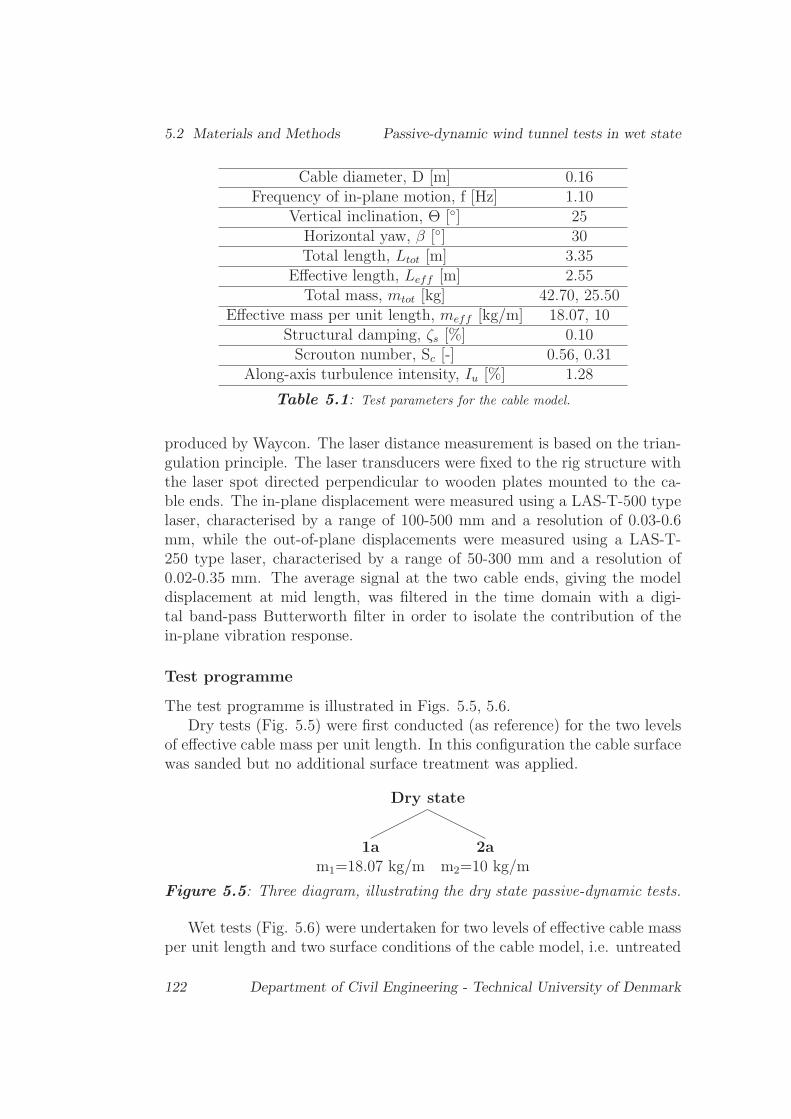
5.2 Materials and Methods Passive-dynamic wind tunnel tests in wet state
Cable diameter, D [m] 0.16Frequency of in-plane motion, f [Hz] 1.10
Vertical inclination, Θ [◦] 25Horizontal yaw, β [◦] 30Total length, Ltot [m] 3.35
Effective length, Leff [m] 2.55Total mass, mtot [kg] 42.70, 25.50
Effective mass per unit length, meff [kg/m] 18.07, 10Structural damping, ζs [%] 0.10Scrouton number, Sc [-] 0.56, 0.31
Along-axis turbulence intensity, Iu [%] 1.28
Table 5.1: Test parameters for the cable model.
produced by Waycon. The laser distance measurement is based on the trian-gulation principle. The laser transducers were fixed to the rig structure withthe laser spot directed perpendicular to wooden plates mounted to the ca-ble ends. The in-plane displacement were measured using a LAS-T-500 typelaser, characterised by a range of 100-500 mm and a resolution of 0.03-0.6mm, while the out-of-plane displacements were measured using a LAS-T-250 type laser, characterised by a range of 50-300 mm and a resolution of0.02-0.35 mm. The average signal at the two cable ends, giving the modeldisplacement at mid length, was filtered in the time domain with a digi-tal band-pass Butterworth filter in order to isolate the contribution of thein-plane vibration response.
Test programme
The test programme is illustrated in Figs. 5.5, 5.6.Dry tests (Fig. 5.5) were first conducted (as reference) for the two levels
of effective cable mass per unit length. In this configuration the cable surfacewas sanded but no additional surface treatment was applied.
Dry state
1am1=18.07 kg/m
2am2=10 kg/m
Figure 5.5: Three diagram, illustrating the dry state passive-dynamic tests.
Wet tests (Fig. 5.6) were undertaken for two levels of effective cable massper unit length and two surface conditions of the cable model, i.e. untreated
122 Department of Civil Engineering - Technical University of Denmark

Passive-dynamic wind tunnel tests in wet state 5.2 Materials and Methods
and coated with a solution of 5% weight Gohsenol KP-08R commercializedby Nippon Gohsei (2012) dissolved in water. For the untreated case, the twosituations of water directly sprayed on the cable model and slowly dryingcable (i.e. with the spray system turned off) were investigated. In the firstcase steady water rivulets appeared on the cable surface, in the second caseonly water droplets.
Wet state
m1=18.07 kg/m
1bsurface treatment,
spray on
no surface treatment
1cspray on
1dspray off(drying)
m2=10 kg/m
2bsurface treatment,
spray on
no surface treatment
2cspray on
2dspray off(drying)
Figure 5.6: Tree diagram, illustrating the wet state passive-dynamic tests.
All tests were conducted for a range of wind velocities from 5 to to 25 m/s,corresponding to Reynolds number, Re = 0.5·105 - 2.7 ·105. For each testedvelocity the aerodynamic damping as well as the peak to peak amplitude ofthe response were evaluated. For wind velocities where the cable vibrationgrew spontaneously, the total damping was evaluated as the slope of the vi-bration growth. For the remaining wind velocities the total damping wasevaluated from free vibration decays obtained after exciting the cable modelmanually, so as to reach an amplitude of vibration in the range of 1D-1.5D.Vibration growths indicated that the aerodynamic damping was negative andlarger in absolute value than the structural damping. Vibration decays in-dicated that the total damping was positive, thus the aerodynamic dampingwas either positive or negative but smaller in absolute value than the struc-tural damping. The aerodynamic damping was evaluated as the differencebetween the total and the structural damping. For both growth and decayevents the total damping is evaluated for the range of vibration amplitude1D-0.10D.
Department of Civil Engineering - Technical University of Denmark 123
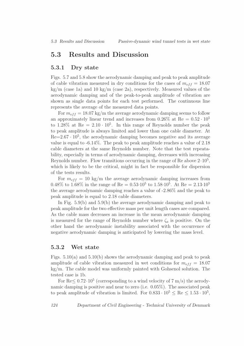
5.3 Results and Discussion Passive-dynamic wind tunnel tests in wet state
5.3 Results and Discussion
5.3.1 Dry state
Figs. 5.7 and 5.8 show the aerodynamic damping and peak to peak amplitudeof cable vibration measured in dry conditions for the cases of meff = 18.07kg/m (case 1a) and 10 kg/m (case 2a), respectively. Measured values of theaerodynamic damping and of the peak-to-peak amplitude of vibration areshown as single data points for each test performed. The continuous linerepresents the average of the measured data points.
Formeff = 18.07 kg/m the average aerodynamic damping seems to followan approximately linear trend and increases from 0.26% at Re = 0.52 · 105to 1.28% at Re = 2.10 · 105. In this range of Reynolds number the peakto peak amplitude is always limited and lower than one cable diameter. AtRe=2.67 · 105, the aerodynamic damping becomes negative and its averagevalue is equal to -6.14%. The peak to peak amplitude reaches a value of 2.18cable diameters at the same Reynolds number. Note that the test repeata-bility, especially in terms of aerodynamic damping, decreases with increasingReynolds number. Flow transitions occurring in the range of Re above 2·105,which is likely to be the critical, might in fact be responsible for dispersionof the tests results.
For meff = 10 kg/m the average aerodynamic damping increases from0.48% to 1.68% in the range of Re = 0.53·105 to 1.58·105. At Re = 2.13·105the average aerodynamic damping reaches a value of -2.86% and the peak topeak amplitude is equal to 2.18 cable diameters.
In Fig. 5.9(b) and 5.9(b) the average aerodynamic damping and peak topeak amplitude for the two effective mass per unit length cases are compared.As the cable mass decreases an increase in the mean aerodynamic dampingis measured for the range of Reynolds number where ζa is positive. On theother hand the aerodynamic instability associated with the occurrence ofnegative aerodynamic damping is anticipated by lowering the mass level.
5.3.2 Wet state
Figs. 5.10(a) and 5.10(b) shows the aerodynamic damping and peak to peakamplitude of cable vibration measured in wet conditions for meff = 18.07kg/m. The cable model was uniformly painted with Gohsenol solution. Thetested case is 1b.
For Re≤ 0.72 ·105 (corresponding to a wind velocity of 7 m/s) the aerody-namic damping is positive and near to zero (i.e. 0.05%). The associated peakto peak amplitude of vibration is limited. For 0.833 · 105 ≤ Re ≤ 1.53 · 105,
124 Department of Civil Engineering - Technical University of Denmark

Passive-dynamic wind tunnel tests in wet state 5.3 Results and Discussion
(a)
(b)
Figure 5.7: Aerodynamic damping (a) and peak to peak amplitude (b) asfunction of Reynolds number in dry conditions, case 1a.
which corresponds to wind velocities in the range of 8 to 15 m/s, the aero-dynamic damping becomes negative and its average reaches a minimum of-0.45%. In this interval of Re the vibration amplitude is growing following anexponential trend until hitting the rig structure where it has to be stoppedmanually. An upper and lower water rivulets are formed on the cable surfaceand oscillate circumferentially (see Fig. 5.19(a)). This is thus identified asthe interval of Reynolds number associated with the occurrence of rain-windinduced vibration.
For higher Reynolds number the aerodynamic damping becomes positiveagain and the peak to peak amplitude of vibration is limited.
Fig. 5.11 shows a time history of cable vibration for Re = 0.96 ·105 (U= 9 m/s). The cable vibration is growing spontaneously until reaching a
Department of Civil Engineering - Technical University of Denmark 125

5.3 Results and Discussion Passive-dynamic wind tunnel tests in wet state
(a)
(b)
Figure 5.8: Aerodynamic damping (a) and peak to peak amplitude (b) asfunction of Reynolds number in dry conditions, case 2a.
peak to peak amplitude of vibration of 2.7D. As the peak to peak amplitudereaches the dynamic rig structure, the cable is stopped manually, so thatthe vibration amplitude is reduced to zero. After being released, the cablevibration starts to grow again. In Fig. 5.11 four consecutive growth eventsare shown.
Fig. 5.12(a) and 5.12(b) shows the aerodynamic damping and peak topeak amplitude of vibration for the cable model with meff = 18.07 kg/m,and untreated surface. The spray system was turned on and an upper andlower steady water rivulets formed on the cable surface (see Fig. 5.19(b)).The test case is 1c.
In this case the aerodynamic damping is positive throughout the wholetested range of Reynolds number and varies from 0.15% at Re=0.55·105 to
126 Department of Civil Engineering - Technical University of Denmark
Passive-dynamic wind tunnel tests in wet state 5.3 Results and Discussion
(a)
(b)
Figure 5.9: Average aerodynamic damping (a) and peak to peak amplitude(b) as function of Reynolds number in dry conditions, case 2a and 2b.
1.20% at Re=2.07·105. The peak to peak amplitude of vibration is near zerofor the whole tested Re range. The cable is thus manifestly stable and thevalues of the aerodynamic damping are very similar to the ones measuredin dry conditions. This indicates the the sole presence of the water rivulets(non-oscillating) is a necessary but not sufficient condition for the instabilityto develop. Their angular oscillation, which is achieved by the occurrenceof the right level of wettability, is fundamental. Note finally, by comparingFigs. 5.19(a) and 5.19(b), that the geometry of the rivulets is completelydifferent for the two cases. When the cable is more wettable the rivulets,become wider.
Figs. 5.13(a) and 5.13(b) show the aerodynamic damping and peak topeak amplitude of vibration for the cable model withmeff = 18.07 kg/m, and
Department of Civil Engineering - Technical University of Denmark 127

5.3 Results and Discussion Passive-dynamic wind tunnel tests in wet state
(a)
(b)
Figure 5.10: Aerodynamic damping (a) and peak to peak amplitude (b) asfunction of Reynolds number in wet conditions, case 1b.
Figure 5.11: Time history of cable vibration, at 9 m/s, case 1b.
128 Department of Civil Engineering - Technical University of Denmark

Passive-dynamic wind tunnel tests in wet state 5.3 Results and Discussion
(a)
(b)
Figure 5.12: Aerodynamic damping (a) and peak to peak amplitude (b) asfunction of Reynolds number in wet conditions, case 1c.
untreated surface. The spray system was turned off and the cable surface wascovered by water droplets (see Fig. 5.19(c)). The test case is 1d. Again, noaerodynamic instability was detected for the tested range of Reynolds num-ber, being the aerodynamic damping positive and the peak to peak amplitudeof vibration near zero. In particular, the aerodynamic damping ranges from0.13% at Re=0.55·105 to 0.94% at Re=2.66·105 and doesn’t follow a lineartrend.
Figs. 5.14(a) and 5.14(b) show the aerodynamic damping and peak topeak amplitude of vibration measured in wet conditions for meff = 10 kg/m.The cable model is uniformly painted with Gohsenol solution. The testedcase is 2b. The aerodynamic damping is positive for Re=0.53·105 to 0.85·105(corresponding to wind velocity of 5 to 8 m/s) and ranges from 0.24% to
Department of Civil Engineering - Technical University of Denmark 129

5.3 Results and Discussion Passive-dynamic wind tunnel tests in wet state
(a)
(b)
Figure 5.13: Aerodynamic damping (a) and peak to peak amplitude (b) asfunction of Reynolds number in wet conditions, case 1d.
0.74%. It becomes negative for Re=0.97·105 to 1.44·105 (wind velocity equalto 9 to 13.5 m/s) and ranges from -1.28% to -0.44%.
Figs. 5.15(a) and 5.15(b) show the aerodynamic damping and peak topeak amplitude of vibration for the cable model with meff = 10 kg/m, anduntreated surface. The spray system was turned on and an upper and lowersteady water rivulets formed on the cable surface, as for case 1c. The testcase is 2c.
As for the higher mass level the aerodynamic damping is positive through-out the whole tested Re range and varies from 0.31% to 2.64% for Re =0.54·105 to 2.15·105. It is thus generally higher than for the respective case1c. The peak to peak amplitude is near zero for the whole Re range.
Figs. 5.16(a) and 5.16(b) show the aerodynamic damping and peak to
130 Department of Civil Engineering - Technical University of Denmark

Passive-dynamic wind tunnel tests in wet state 5.3 Results and Discussion
(a)
(b)
Figure 5.14: Aerodynamic damping (a) and peak to peak amplitude (b) asfunction of Reynolds number in wet conditions, case 2b.
peak amplitude of vibration for the cable model with meff = 10 kg/m, anduntreated surface. The spray system was turned off and the cable surfacewas covered by water droplets, as for case 1d. The tested case is 2d. Theaerodynamic damping is positive and ranges from 0.13% at Re=0.55·105 to1.49% at Re = 2.14 · 105. It is thus generally higher than for the respectivecase 2d. The peak to peak amplitude of vibration is near zero for the wholeRe range.
Fig. 5.17 shows the average aerodynamic damping (5.17(a)) and peak topeak amplitude vibration (5.17(b)) for cases 1b, 1c, 1d (meff = 18.07 kg/m)and 2b, 2c, 2d (meff = 10 kg/m).
Fig. 5.18 shows the average aerodynamic damping for meff = 18.07kg/m (5.18(a)) and meff = 10 kg/m (5.18(b)) for cases 1a, 1c, 1d (meff
Department of Civil Engineering - Technical University of Denmark 131

5.3 Results and Discussion Passive-dynamic wind tunnel tests in wet state
(a)
(b)
Figure 5.15: Aerodynamic damping (a) and peak to peak amplitude (b) asfunction of Reynolds number in wet conditions, case 2c.
= 18.07 kg/m) and 2a, 2c, 2d (meff = 10 kg/m). It is observed that theaerodynamic damping in dry conditions and in presence of steady upperand lower rivulet are very similar for both mass levels. Lower values of theaerodynamic damping occur for the cable covered by water droplets.
132 Department of Civil Engineering - Technical University of Denmark

Passive-dynamic wind tunnel tests in wet state 5.4 Conclusion
(a)
(b)
Figure 5.16: Aerodynamic damping (a) and peak to peak amplitude (b) asfunction of Reynolds number in wet conditions, case 2d.
5.4 Conclusion
Passive-dynamic wind tunnel tests were undertaken for a section of an in-clined and yawed full-scale plain bridge cable model. Tests were performedfor varying cable surface conditions, i.e. in the dry and wet state, for varyinglevels of surface wettability, and cable masses per unit length. Tests helpedto better understand the instability mechanisms of bridge cable sections indry and wet surface conditions.
In particular, galloping-type instability was detected in dry conditions inthe critical Reynolds number range. Here the aerodynamic damping becamenegative and was accompanied by large amplitude vibrations. A decreasein the cable mass in dry conditions provoked an anticipation of the critical
Department of Civil Engineering - Technical University of Denmark 133

5.4 Conclusion Passive-dynamic wind tunnel tests in wet state
(a)
(b)
Figure 5.17: Average aerodynamic damping (a) and peak to peak amplitude(b) as function of Reynolds number in wet conditions, cases 1b, 1c, 1d and2b, 2c, 2d.
Reynolds number and thus of the aerodynamic instability.
Under the effects of wind and rain, the cable model underwent differenttypes of instability mechanisms, depending on the level of surface wettabilityand of mass. RWIV instability was observed only when the cable surfacewas characterised by an increased level of wettability, for all tested mass lev-els. The instability occurred only for a limited range of Reynolds numberand was again characterized by the occurrence of large amplitude vibrationsaccompanied by negative aerodynamic damping. No RWIV instability wasexperienced for the cable model with very low wettability, either in presenceof steady water rivulets, induced by a uniform water flow, or in presence ofdroplets, in the drying state. In particular, the aerodynamic damping of the
134 Department of Civil Engineering - Technical University of Denmark

Passive-dynamic wind tunnel tests in wet state 5.4 Conclusion
(a)
(b)
Figure 5.18: Average aerodynamic damping as function of Reynolds num-ber in wet conditions for cases 1a, 1c, 1d (a) and 2a, 2c, 2d (b)
cable model in dry conditions and in wet conditions, in presence of steadywater rivulets, were nearly equal for the range of Re up to 2·105 for bothmass levels. For higher Re, the aerodynamic damping in dry conditions be-came negative and was accompanied by large amplitude vibrations, while inwet conditions it was still positive and the vibration was limited in ampli-tude. This implies that in the subcritical Re range the presence of steadyrivulets doesn’t lead to any kind of instability and the cable behaves as indry conditions. The presence of the rivulets had instead a damping effectat high velocities; in fact, differently from the dry cable, the wet cable withsteady rivulets was stable at high Reynolds numbers. In the drying statethe cable model was characterized by a time dependent surface roughness,which leaded to a time dependency of the aerodynamic damping at a specific
Department of Civil Engineering - Technical University of Denmark 135
5.4 Conclusion Passive-dynamic wind tunnel tests in wet state
Reynolds number. Finally in wet conditions, at the right level of surfacewettability, the range of Re where the aerodynamic instability occurs is re-stricted by decreasing the cable mass. Thus at lower mass conditions, theoscillating water rivulets has a major damping effect than for higher mass.Note that for meff = 18.07 kg/m, occurs for a limited range of wind veloci-ties which is narrower than for the meff = 18.07 kg/m. Decreasing the cablemass in wet conditions thus stabilizes the cable’s aerodynamic behaviour forwind velocities of in the range of 8 to 9 m/s and 13.5 to 15 m/s.
136 Department of Civil Engineering - Technical University of Denmark

Passive-dynamic wind tunnel tests in wet state 5.4 Conclusion
(a)
(b)
(c)
Figure 5.19: View of the upper rivulet for the Gohsenol treated (a) anduntreated (b) cable surface, and droplets formations for the untreated cablesurface.
Department of Civil Engineering - Technical University of Denmark 137

5.4 Conclusion Passive-dynamic wind tunnel tests in wet state
138 Department of Civil Engineering - Technical University of Denmark

Bibliography
Acampora, A., Georgakis, C.T., 2011. Recent monitoring of the ØresundBridge: Observations of rain-wind induced cable vibrations. In: 13th In-ternational Wind Engineering Conference,Amsterdam.
Bosdogianni, A., Olivari, D., 1996. Wind- and rain-induced oscillations ofcables of stayed bridges. J. Wind Eng. Ind. Aerodyn. 64, 171-185.
Cosentino, N., Flamand, O., Ceccoli, C., 2003a. Rain-wind induced vibrationof inclined stay cables. Part I: Experimental investigation and physicalexplanation. J. Wind and Structures. 6, 471-484.
Eriksen, M.B., 2012. Passive-Dynamic Wind Tunnel Tests of Rain-Wind In-duced Vibrations. Technical Report.
Flamand, O., 1995. Rain-wind induced vibrations of cables. J. Wind Eng.Ind. Aerodyn. 57, 353-362.
Georgakis, C.T., Koss, H.H., Ricciardelli, F., 2009. Design specifications fora novel climatic wind tunnel for testing of structural cables. In: 8th Inter-national Symposium on Cable Dynamics, Paris, pp. 333-340.
Hardy, C., Bourdon, P., 1979. The influence of spacer dynamic propertiesin the control of bundle conductor motion. IEEE PES Summer Meeting,Vancouver.
Hikami, Y., Shiraishi, N., 1988. Rain-wind induced vibrations of cables incable stayed bridges. J. Wind Eng. Ind. Aerodyn. 29, 409-418.
Larose, G.L., Smitt, L.W., 1999. Rain/Wind induced vibration of parallelstay cables. In: IABSE Conference, Cable-Stayed Bridges - Past, Presentand Future, Malmo, Sweden, pp - .
Lemaitre, C., de Langre, E., Hemon, 2010. Rainwater rivulets running on astay cable subject to wind. European Journ. of Mechanics B/Fluids 29,251-258.
139

BIBLIOGRAPHY BIBLIOGRAPHY
Liu, Q., Wang, Y., Zheng, Y.,Ma, W., 2012. Experimental study on therelation of water rivulet-Reynolds number effect-cable vibration. In: 7thInternational Colloquium on Bluff Body Aerodynamics and Applications,Shanghai, China.
Ni, Y.Q., Wang, X.Y., Chen, Z.Q., Ko, J.M., 2007. Field observations ofrain-wind-induced cable vibration in cable-stayed Dongting Lake Bridge.J. Wind Eng. Ind. Aerodyn. 95, 303-328.
Nippon Gohsei, How To Use GOHSENOL, October 2012.
Noisternig, J.F., 2000. Carbon Fibre Composites as Stay Cables for Bridges.Applied Composite Materials 7, 139-150.
Yoshimura, T., Tanaka, T., Sasaki, N., Nakatani, S., Higa, S., 1988. Rain-wind induced vibration of the cables of the Aratsu Bridge. In: 10th Nat.Conf. on Wind Engineering, Tokyo, pp. 127-132.
Wianecki, J., 1979. Cable wind excited vibrations of cable-stayed bridges.In: 5th Int. Conf. of Wind Eng., Colorado, Oxford-New York, PergamonPress, pp. 1381-1393
Zuo, D., Jones, N.P., Main, J.A., 2008. Field observation of vortex- and rain-wind-induced stay-cable vibrations in a three-dimensional environment. J.Wind Eng. Ind. Aerodyn. 96, 1124-1133.
Zuo, D., Jones, N.P., 2010. Interpretation of field observations of wind-a ndrain-wind-induced stay cable vibrations. J. Wind Eng. Ind. Aerodyn. 98,73-87.
140 Department of Civil Engineering - Technical University of Denmark
Chapter 6
Analytical model
The results presented in this chapter are taken from the paper Quasi-steady3 DOF aerodynamic instability criterion for galloping and static divergenceof an inclined/yawed prism, to be submitted to the Journal of Fluids andStructures.
Abstract
A generalized quasi-steady three-degrees-of-freedom analytical model, capa-ble of predicting the linear aerodynamic instability of a prism with genericcross-section, immersed in a turbulent wind flow is proposed. The threedegrees-of-freedom refer to the two orthogonal displacements, perpendicularto the body’s axis, plus the rotation about the longitudinal body axis. Themodel incorporates the inertial coupling, i.e. the non coincidence between thecenter of mass and the center of rotation between the degrees-of-freedom. Italso allows for variation of the force coefficients, i.e. drag, lift, and moment,with Reynolds number based on the relative flow velocity, with relative angle-of-attack, and relative cable-wind angle. The aerodynamic forces acting onthe structure are linearized about the static equilibrium configuration, i.e.about zero structural velocities along the three degrees-of-freedom, steadystructural rotation about the body’s longitudinal axis, and about the steadycomponent of the total wind velocity. Based on the analytical solution of theeigenvalue problem, by applying the Routh-Hurwitz criterion, an expressionof the galloping- and static divergence-type instability condition is derived.Additionally, a numerical solution of the minimum structural damping andstructural stiffness required to prevent the same aerodynamic instabilities aregiven.
A practical application of the 3-DoFs instability model for the an iced
141

6.1 Introduction Analytical model
conductor section is finally proposed. The quasi-steady drag, lift and momentcoefficients of the conductor were found in the existing literature, as well asthe regions of aerodynamic instability, derived from passive-dynamic windtunnel tests performed on the same conductor model. Maps of galloping andstatic divergence instability are presented for the test case and compared withpredictions based on existing 1-DoF, 2-DoFs and 3-DoFs analytical models.It was found that the present model gives the best prediction of the regionsof instability, when compared with dynamic test results.
6.1 Introduction
When a structure oscillates in steady flow, the flow field relative to thestructure also oscillates, thus producing fluctuating aerodynamic force com-ponents, which can be coupled either linearly or non linearly, to the body’sstructural acceleration (a), velocity (b) or displacement/rotation (c), (Blevinsand Iwan, 1975). In the first case, (a), a variation of the body’s effective massoccurs. Nevertheless, as the mass of the surrounding air is normally negligi-ble in comparison to the mass of the structural body, this variation is seldomsufficient to affect the system’s stability. In the second case, (b), a variationof the body’s effective damping occurs. This can eventually vanish whenthe flow field generates negative aerodynamic damping, equal in absolutevalue to the structural damping. This phenomenon can initiate instabilitiesof dynamic type, such as galloping, which are characterized by the occur-rence of large amplitude vibrations, mostly in the cross-wind direction, atlow frequencies. The galloping instability is of interest for a large class ofbluff bodies, slender and with non-circular cross-section, typical examples be-ing power line conductors or bridge cable sections covered by ice accretions,which experience flow separation and associated changes in the drag and liftcoefficients at specific Reynolds numbers. In the third case, (c), a variation inthe body’s effective stiffness (frequency) is experienced. In particular, if theflow field generates negative aerodynamic stiffness, equal in absolute value tothe structural stiffness, the body’s effective stiffness becomes zero, causing aform of aerodynamic instability known as divergence. This instability is ofstatic type and occurs for streamlined bodies, such as airfoil wings, when theyexperience an elastic rotation not counteracted by the body’s torsional stiff-ness. All instabilities start suddenly, when a critical wind velocity is reached,and are characterized by a rapid increase in the structural displacements asthe wind velocity increases, (Davenport and Novak, 2002).
Bluff-body aerodynamic instabilities of galloping-type have been modeled,based on the (QS) theory. According to the theory the aerodynamic forces
142 Department of Civil Engineering - Technical University of Denmark

Analytical model 6.1 Introduction
on structures are expressed as nonlinear memoryless transformation of theflow-structure relative velocity and the angle-of-attack, which are variable intime due to the oscillation of the body and the presence of the turbulence ofthe oncoming flow (Kareem and Wu, 2013). The non linearities which arisein the aerodynamic force equations are normally approximated by means ofpolynomial expressions, i.e. for example by a Taylor series expansion, (De-noel and Degee, 2006), or by an optimization procedure aimed at minimizingsome error measure, (Carassale and Kareem, 2010). The QS assumption isthus satisfied when the characteristic fluid-dynamic time scale of the velocityfluctuations in the wake of the body are much faster than the time scale ofthe body’s oscillation. In fact, as galloping normally occurs at low reducedfrequencies, the associated aerodynamic forces can be assumed as steady,and the susceptibility of a generic cross-section to galloping instability canbe assessed by means of the aerodynamic force coefficients measured in staticconditions.
First galloping instability models were based on the assumption that astructure responds to the aerodynamic excitation as a single DoF. Across-flowand along-flow instability criteria for a bluff body in cross-flow, known as 1-DoF galloping and drag crisis were derived by Den Hartog (1956) and Martinet al. (1981), respectively. In these models the aerodynamic force coefficientswere assumed to only vary with angle-of-attack, (Den Hartog, 1956), andwith Reynolds number, (Martin et al., 1981). Macdonald and Larose (2006)derived a generalized quasi-steady 1-DoF instability model, where the aero-dynamic forces accounted for arbitrary orientation of the body’s longitudinalaxis with respect to the flow velocity (cable-wind angle), as well as orienta-tion of the vibration axis with respect to the projection of the wind velocityin the body’s cross-sectional plane (angle-of-attack). Moreover, the depen-dency of the force coefficients on the Reynolds number, was accounted for.The Reynolds number was evaluated based on the vectorial combination ofthe normal and axial flow velocities, as both affect the force coefficients in thecritical range. The dependency of the force coefficients on the combinationof the three latter parameters was neglected by previous galloping analyses,but it is fundamental for certain classes of bluff bodies, such as bridge staycables. The model developed by Macdonald and Larose (2006) thus predictsdifferent types of aerodynamic instabilities, and can be reduced, for specificcombinations of the input parameters, to the Den Hartog galloping and dragcrisis criteria.
Following analyses emphasized how real structures respond to aerody-namic excitation as multi-DoFs systems. Given the increased complexity ofthe analytical solution for a whole coupled 3-DoFs system, the instabilitymodels available in the literature mostly focus on reduced 2-DoFs systems.
Department of Civil Engineering - Technical University of Denmark 143

6.1 Introduction Analytical model
These models are realistic only when the neglected mode has a frequencywhich is far away from the frequencies of the accounted DoFs. Jones (1992)analyzed the response of a bluff body in cross-flow, for coupled translationalgalloping, i.e. in vertical and horizontal motion. The force coefficients weremodeled as function of the only angle-of-attack. By assuming that the vi-bration frequencies of the two selected modes were coincident (tuned case),a closed form solution to the fourth-order characteristic equation governingthe instability problem was obtained. On the other hand, if this assump-tion is removed, numerical methods must be employed for the solution ofthe eigenvalue problem’s characteristic equation; consequently only specificproblems can be studied and an exhaustive description of all the possiblecritical conditions for varying system parameters is difficult to be obtained,(Luongo and Piccardo, 2005). By performing passive-dynamic wind tunneltests, Cheng et al. (2008a) demonstrated that a 2-DoFs-type translatory gal-loping instability can also occur for bridge stay cables whose longitudinalaxis is inclined/yawed with respect to the wind direction. The observed in-stability, known as dry inclined galloping, occurs in the critical Re range,and is characterized by major vibration components in the in-plane direc-tion, with small vibration components in the out-of-plane direction, leadingto elliptical trajectories. In this connection, Macdonald and Larose (2008a)and Macdonald and Larose (2008a) derived a 2-DoFs instability model ableto predict the structural damping necessary to avoid galloping instability ofan inclined/yawed cylinder moving in a 2D plane. As in the previous model,see (Macdonald and Larose, 2006), the force coefficients were modeled asfunction of the relative Reynolds number, cable-wind angle, and angle-of-attack. As Jones (1992), Macdonald and Larose (2008a) derived a closedform solution for the tuned case and Macdonald and Larose (2008b) deriveda numerical solution for the detuned cases.
? pointed out that bluff bodies, whose center of mass doesn’t coincidewith the center of rotation, such as eccentrically iced conductors, can un-dergo instabilities associated with the torsional DoF, either of 1-DoF-typeor multi-DoFs-type. The 1-DoF-type instability occurs when the torsionalaerodynamic damping becomes negative and higher in absolute value thanthe inherent structural torsional damping; in this condition the torsionalmode becomes self-exciting and the cylinder will oscillate at a frequency de-termined by the effective torsional stiffness and the polar moment of inertia.Multi-DoFs instability occurs when the torsional frequency approaches oneof the resonant vertical or horizontal galloping frequencies; in this condition,the two lateral modes become excited through the coupled force terms. Forice-accreted cable conductors, it is apparent that the torsional stiffness andfrequency are affected by the eccentric mass of the ice and by the slope of
144 Department of Civil Engineering - Technical University of Denmark
Analytical model 6.1 Introduction
the moment coefficient against angle-of-attack. In particular, the torsionalfrequency is reduced when center of the eccentric ice mass is placed above therotational center of the conductor and increased when this is placed below.Similarly, the torsional frequency is reduced when the slope of the aerody-namic moment is positive and increased when it is negative. The gallopingresponse of a 2-DoFs system, vibrating in the across-flow and torsional di-rection, was investigated by Blevins and Iwan (1975) and Yu et al. (1992).Blevins and Iwan (1975) assumed that the mass-spring-damper system isuncoupled, i.e. the center of mass coincides with the elastic axis; this simpli-fying assumption was not made by Yu et al. (1992). Yu et al. (1993) extendedthe 2-DoFs model developed by Yu et al. (1993) to 3-DoFs, by additionallyaccounting of the along-flow vibration component. The models developedby Blevins and Iwan (1975), Yu et al. (1992) and Yu et al. (1993) are validfor cylinders in cross-flow. In all these models, the aerodynamic forces werelinearized about angle-of-attack, while neglecting the Reynolds number de-pendency. A quasi-steady 2-DoF sectional model for galloping instability inthe along- and across-flow direction was developed by Carassale et al. (2004).The model is valid for cylinders with generic orientation with respect to thewind flow, i.e. inclined/yawed. Similarly to Blevins and Iwan (1975) and Yuet al. (1992), Carassale et al. (2004) linearized the aerodynamic forces onlyabout angle-of-attack.
Stoyanoff (2001) developed a 3-DoFs model valid for prisms with genericcross-section in cross-flow, such as bridge decks or towers. The total aerody-namic forces were modeled as the summation of the self-excited forces, i.e.aerodynamic damping and stiffness proportional terms, and the buffetingforces. The Reynolds number dependency of the force coefficients was ne-glected. Gjelstrup and Georgakis (2011) derived a 3-DoFs model for gallopinginstability of a bluff body with generic attitude to the wind flow. The modelincluded the inertial coupling between the the 3-DoFs. The aerodynamicforces were represented following the same approach as adopted by Macdon-ald and Larose (2006) and Macdonald and Larose (2008a), Macdonald andLarose (2008b), i.e. by modeling the dependency of the force coefficients onthe relative cable-wind angle, angle-of-attack and Reynolds number, and werelater linearized only about zero structural velocities neglecting the expansionabout the displacements. This leads to the elimination of all aerodynamicstiffness terms. Such simplification is valid only for compact sections (Gjel-strup and Georgakis, 2011).
The role of the wind turbulence on the aerodynamic instability of pris-matic bodies has seldom been modeled analytically. Nevertheless, turbulenteddies are most effective in altering the flow structure around such bod-ies and thus affect their inherent aerodynamic stability. In particular, the
Department of Civil Engineering - Technical University of Denmark 145

6.1 Introduction Analytical model
main effect of the small-scale turbulence is to cause earlier reattachment ofthe flow through enhanced mixing in the shear layers. Turbulence in therange of the body’s scale can enhance or weaken vortex shedding depend-ing on the body’s geometry, (Kareem and Wu, 2013). Effects of small-scalewind turbulence were considered by Symes and Macdonald (2006), who ex-panded 1-DoF analytical model developed by Macdonald and Larose (2006),by applying turbulence intensity corrections on both Reynolds number andassociated force coefficients. Corrections were based on ESDU. Recently,Raeesi et al. (2013) proposed a 1-DoF instability model for inclined circularcylinders where the effect of small scale turbulence was included by meansof an unsteady wind model. The model was developed by applying DiscreteWavelet Transform to a set of field wind data. The large scale turbulence,which changes more slowly, generates a variation in the wind velocity and inthe associated aerodynamic loading. The load variation can produce randomforced vibration which can generate a type of instability named as buffeting.The impact of large-scale turbulence was included by Symes and Macdonald(2007) in a 1-DoF analytical model valid for inclined prisms.
A generalized quasi-steady 3-DoFs analytical model, capable of predictingthe aerodynamic instability of a prism with generic cross-section, immersedin turbulent wind flow, is here proposed. The model accounts for the in-ertial coupling between the 3-DoFs, and allows for variation of the forcecoefficients, i.e. drag, lift, and moment, with Reynolds number based on therelative flow velocity, with relative angle-of-attack, and relative cable-windangle. The aerodynamic forces acting on the prism are modeled as non linearfunction of the prism’s structural velocity along the 3 DoFs, of the structuralrotation about the longitudinal axis, as well of the total wind velocity, whichcomprises a steady component and nil-mean fluctuating components. Theaerodynamic forces are linearized about zero structural velocities, steadystructural rotation and about the steady component of the total wind ve-locity. The equations of motion are written by following the Euler-Lagrangemethod. Later, they are expressed in the state space representation. Basedon the analytical solution of the eigenvalue problem, by applying the Routh-Hurwitz criterion, an expression of the galloping- and static divergence-typeinstability condition is derived. Additionally, a numerical solution of theminimum structural damping and structural stiffness required to prevent thesame aerodynamic instabilities are given.
An application of the 3-DoFs analytical model is proposed in order tostudy the galloping and static divergence stability conditions of two sepa-rate test cases, i.e. an ice-accreted model of a cable conductor in cross flow,(Chabart and Lilien, 1998). For the ice accreted cable in cross flow a compar-ison of the regions of galloping instability derived analytically, with results
146 Department of Civil Engineering - Technical University of Denmark

Analytical model 6.2 Linearization of the aerodynamic and mechanical model
of passive-dynamic wind tunnel tests undertaken for the same conductormodel, (Chabart and Lilien, 1998), revealed that the present model providesan improved prediction of the regions of galloping instability in comparisonto existing models. Stability maps of galloping and static divergence werederived. It was found that for selected ranges of angle-of-attack and Reynoldsnumber, the ice accreted cable in cross-flow can undergo both galloping andstatic divergence instability. An increase in the structural damping ratioalong all DoFs helps to reduce the amplitude of the regions of gallopinginstability, while it doesn’t produce any effect on the regions of static diver-gence instability. A reduction of the structural rotational stiffness reducesthe amplitude of the regions of both galloping and static divergence insta-bility. On the other hand a reduction of the along-wind structural stiffnessreduces the regions of galloping instability but has no effect on the staticdivergence.
6.2 Linearization of the aerodynamic and me-
chanical model
6.2.1 Flow around fixed inclined prism
A prism of generic section is immersed in a conventional turbulent wind field.This is modeled by a mean wind velocity component, U , and fluctuatingwind velocity components along three othrogonal directions, u(t), v(t), w(t).A global reference system (X, Y, Z) is defined, where the X, Y axes lay ona horizontal plane and are parallel to U , u(t) and v(t), respectively, while Zis vertical, and parallel to w(t), see Fig. 6.1. The total wind velocity U(t) isgiven by
U(t) = U+ U(t) =[U 0 0
]T+
[u(t) v(t) w(t)
]T(6.1)
The typical attitude in the flow of a prism is given by an inclination Θ, i.e. theangle between the body’s longitudinal axis and its projection in the horizontalplane, and a yaw angle β, i.e. the angle between the free-stream velocity Uand the projection of the body’s axis in the horizontal plane. In general,for civil engineering applications, the inclination is a physical/geometricalcharacteristic, while the yaw depends on the wind direction. A local referencesystem for the prism (x, y, z) is introduced, where x, y belong to its cross-sectional plane and z is parallel to the prism’s longitudinal axis, see Fig.6.2. If the prism is considered to be initially oriented parallel to the globalZ axis, so that the local and global reference systems are coincident, the
Department of Civil Engineering - Technical University of Denmark 147

6.2 Linearization of the aerodynamic and mechanical model Analytical model
inclined/yawed configuration is obtained after a sequence of two elementalrotations. The first one is a rotation about the Y axis of entity (π/2 − Θ),while the second is a rotation about the Z axis of entity −β.
The total wind vector in the rotated local reference system for the prismis given by
Ur(t) = RY (π/2−Θ)RZ(−β)U(t) =
=
⎡⎣ sinΘ cos β (U + u(t)) + sinΘ sin βv(t) + cosΘw(t)− sin β (U + u(t)) + cos βv(t)
− cosΘ cos β (U + u(t))− cosΘ sin βv(t) + sinΘw(t)
⎤⎦ (6.2)
where RY (π/2 − Θ), RZ(−β) are the rotation matrices around the axis Yand Z, respectively.
The total component of the wind velocity in the prism’s section, namednormal flow velocity, UN(t), is given by:
UN(t) =
√(Ur,1(t))
2 + (Ur,2(t))2 =
=
√√√√ (sinΘ cos β (U + u(t)) + sinΘ sin βv(t) + cosΘw(t))2 +
+ (− sin β (U + u(t)) + cos βv(t))2
(6.3)
The component of the wind velocity along the prism’s longitudinal axis,known as axial wind velocity, is:
UA(t) = Ur,3(t) = − cosΘ cos β (U + u(t))−cosΘ sin βv(t)+sinΘw(t) (6.4)
The angle Φ(t) between the prism’s axis and the free-stream velocity Uis given by:
Φ(t) = arccos(|UA(t)|U + u(t)
) =
= arccos(|− cosΘ cos β (U + u(t))− cosΘ sin βv(t) + sinΘw(t)|
U + u(t))
(6.5)A second local reference system (x′, y′, z) is chosen for the prism, so that
the local axis x′ is parallel to the direction of the normal wind velocity UN(t),see Figs. 6.1, 6.2. The wind velocity vector in the (x′, y′, z) reference systemis:
Ur′(t) =[UN(t) 0 UA(t)
]T(6.6)
The angle between UN(t) and the plane containing the prism’s longitudi-nal axis and its horizontal projection, is:
αs(t) = arccosUr,1(t)
UN(t)(6.7)
148 Department of Civil Engineering - Technical University of Denmark

Analytical model 6.2 Linearization of the aerodynamic and mechanical model
Figure 6.1: 3D geometry of the structural member.
6.2.2 Flow around moving inclined prism
The model allows for the motion of the prism along three degrees of freedom(3 DOFs) represented by the vector
q(t) =[ξ(t) η(t) θ(t)
]T(6.8)
where ξ(t), η(t) are two orthogonal displacements belonging to a plane withgeneric spacial orientation with respect to the prism’s cross section and θ(t)is the rotation about the prism’s longitudinal axis. Most commonly, as inthis analysis, the displacements ξ(t) and η(t), are assumed to be parallelto the vertical in-plane and out-of-plane directions, x and y, respectively.The structural velocity and acceleration, i.e. given by the first and secondtime derivatives of the displacement vector q(t), are indicated as q(t) andq(t), respectively. The cross-radial tangential velocity varies in intensity anddirection along the prism’s cross-sectional boundary, due to the effect of θ(t).In fact, its intensity is given by ∣∣∣R ∧ θ(t)
∣∣∣ (6.9)
where R is the distance of a generic point located on the prism’s sectionboundary to the shear center (or center of rotation). The direction is tangentto the prism’s cross-section at the specific point of evaluation. FollowingBlevins (1977), the velocity field on the cross section’s boundary is thusapproximated by choosing a reference point, which is representative of thenet flow field. Normally this point is located at the leading edge, i.e. atdistance Rδ from the shear center and at angular distance δ from the x′ localaxis. Alternative to this approach is to perform a full series of dynamic testsin order to characterize the forces on the rotating cross-section.
Department of Civil Engineering - Technical University of Denmark 149

6.2 Linearization of the aerodynamic and mechanical model Analytical model
Figure 6.2: Plane normal to the prism’s axis.
The angle ϕ(t) is defined as
ϕ(t) = αs(t)− θ(t) =
= arctan
( − sin β (U + u(t)) + cos βv(t)
sinΘ cos β (U + u(t)) + sinΘ sin βv(t) + cosΘw(t)
)− θ(t)
(6.10)The vector qR(t), defined as
qR(t) = Rz (−ϕ(t)) q(t) + ω(t) ∧Rδ =
=
⎡⎣ cosϕ(t) sinϕ(t) 0− sinϕ(t) cosϕ(t) 0
0 0 1
⎤⎦⎡⎣ξ(t)η(t)
θ(t)
⎤⎦+
⎡⎣ 00
θ(t)
⎤⎦ ∧⎡⎣Rδ cos δRδ sin δ
0
⎤⎦=
⎡⎣ ξ(t) cosϕ(t) + η(t) sinϕ(t)−Rδθ(t) · sin δ−ξ(t) · sinϕ(t) + η(t) cosϕ(t)−Rδθ(t) cos δ
θ(t)
⎤⎦(6.11)
represents the structural velocity in the (x′, y′, z) local reference system,where qR,1, qR,2 are the structural velocities in the prism’s cross sectionalplane, parallel to the x′ and y′ directions, while qR,3 represents the angularvelocity.
The relative wind velocity UR(t) in the (x′, y′, z) local reference systemis the difference between the total wind velocity Ur′(t) and the components
150 Department of Civil Engineering - Technical University of Denmark

Analytical model 6.2 Linearization of the aerodynamic and mechanical model
of qR(t) in the prism’s cross-section.
UR(t) = Ur′(t)− qR(t) =[UN(t) 0 UA(t)
]T − [qR,1 qR,2 0
]T=
⎡⎣UN(t)− ξ(t) cosϕ(t)− η(t) sinϕ(t) +Rδθ(t) · sin δξ(t) · sinϕ(t)− η(t) cosϕ(t) +Rδθ(t) cos δ
UA(t)
⎤⎦(6.12)
The intensity UNR(t) of relative normal wind velocity is
UNR(t) =√
(UR,1)2 + (UR,2)2
=
√√√√√√(UN(t)− ξ(t) cosϕ(t)− η(t) sinϕ(t) +Rδθ(t) · sin δ
)2
+(ξ(t) sinϕ(t)− η(t) cosϕ(t) +Rδθ(t) · cos δ
)2
(6.13)The angle between UNR(t) and the local x axis is
αR(t) = ϕ(t) + arctan
(UR,2
UR,1
)= arctan
( − sin β (U + u(t)) + cos βv(t)
sinΘ cos β (U + u(t)) + sinΘ sin βv(t) + cosΘw(t)
)− θ(t)+
+ arctan
(ξ(t) sinϕ(t)− η(t) cosϕ(t) +Rδθ(t) cos δ
U · sinφ− ξ(t) cosϕ(t)− η(t) sinϕ(t) +Rδθ(t) sin δ
)(6.14)
Following eq. 6.5, the relative cable-wind angle ΦR(t) is:
ΦR(t) = arccos
( |UA(t)||UR(t)|
)=
= arccos
( |− cosΘ cos β (U + u(t))− cosΘ sin βv(t) + sinΘw(t)||UR(t)|
)(6.15)
The linearized expression of UR(t), ΦR(t), αR(t) is:
b(q(t), θ(t),U(t)) =[UR(q, θ(t),U(t)) αR(q, θ(t),U(t)) ΦR(q, θ(t),U(t))
]T(6.16)
Department of Civil Engineering - Technical University of Denmark 151

6.2 Linearization of the aerodynamic and mechanical model Analytical model
where
UR(q, θ(t),U(t)) = U + u(t)− sinΦ(cos ϕξ(t) + sin ϕη(t)−Rδ sin δθ(t)
)αR(q, θ(t),U(t)) = ϕ+
1
U(sin2 Θ+ tan2 β)
(sinΘ(1 + tan2 β)v(t) +
cosΘ sin β
cos2 βw(t)
)+
1
U sinΦ
(sin ϕξ(t)− cos ϕη(t)−Rδ cos δθ(t)
)− θ(t)
ΦR(q, θ(t),U(t)) = − 1
U sinΦ(cosΘ sin βv(t)− sinΘw(t))
+sinΘ
UΦ− cosΦ
U
(cos ϕξ(t) + sin ϕη(t)−Rδ sin δθ(t)
)(6.17)
Detailed derivation of eq. 6.17 is reported in Appendix A.2.
6.2.3 Aerodynamic forces
The aerodynamic force coefficients, C depend on the Reynolds number, Re,wind angle-of-attack, α, and cable-wind angle, Φ. This dependency can beexpressed as
C(d) =[Cx′(d) Cy′(d) DCMz(d)
]T(6.18)
where the vector d is obtained by applying the transformation
d(q(t), θ(t),U(t)) = Tb(q(t), θ(t),U(t))
=
⎡⎣ReR(q(t), θ(t),U(t))αR(q(t), θ(t),U(t))ΦR(q(t), θ(t),U(t))
⎤⎦ (6.19)
T is the transformation matrix
T =
⎡⎢⎣D
ν0 0
0 1 00 0 1
⎤⎥⎦ (6.20)
and ReR is the Reynolds number based on UR. Detailed derivation of eq.6.19 is reported in Appendix A.2.
The aerodynamic forces Fa per unit length along the x′R, y
′R axes, and
152 Department of Civil Engineering - Technical University of Denmark
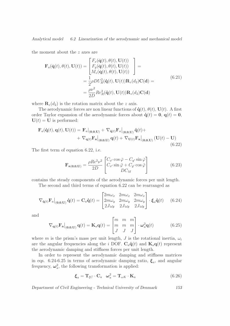
Analytical model 6.2 Linearization of the aerodynamic and mechanical model
the moment about the z axes are
Fa(q(t), θ(t),U(t)) =
⎡⎣Fx(q(t), θ(t),U(t))Fy(q(t), θ(t),U(t))Mz(q(t), θ(t),U(t))
⎤⎦ =
=1
2ρDU2
R(q(t),U(t))Rz(d2)C(d) =
=ρν2
2DRe2R(q(t),U(t))Rz(d2)C(d)
(6.21)
where Rz(d2) is the rotation matrix about the z axis.The aerodynamic forces are non linear functions of q(t), θ(t), U(t). A first
order Taylor expansion of the aerodynamic forces about q(t) = 0, q(t) = 0,U(t) = U is performed:
Fa(q(t),q(t),U(t)) = Fa|(0,0,U) + ∇q(t)Fa
∣∣(0,0,U)
q(t)+
+ ∇q(t)Fa
∣∣(0,0,U)
q(t) + ∇U(t)Fa
∣∣(0,0,U)
(U(t)−U)
(6.22)The first term of equation 6.22, i.e.
Fa(0,0,U) =ρRe2ν2
2D
⎡⎣Cx′ cos ϕ− Cy′ sin ϕCx′ sin ϕ+ Cy′ cos ϕ
DCM
⎤⎦ (6.23)
contains the steady components of the aerodynamic forces per unit length.The second and third terms of equation 6.22 can be rearranged as
∇q(t)Fa
∣∣(0,0,U)
q(t) = Caq(t) =
⎡⎣2mωx 2mωx 2mωx
2mωy 2mωy 2mωy
2Jωθ 2Jωθ 2Jωθ
⎤⎦ · ξaq(t) (6.24)
and
∇q(t)Fa
∣∣(0,0,U)
q(t) = Kaq(t) =
⎡⎣m m mm m mJ J J
⎤⎦ · ω2aq(t) (6.25)
where m is the prism’s mass per unit length, J is the rotational inertia, ωi
are the angular frequencies along the i DOF. Caq(t) and Kaq(t) representthe aerodynamic damping and stiffness forces per unit length.
In order to represent the aerodynamic damping and stiffness matricesin eqs. 6.24-6.25 in terms of aerodynamic damping ratio, ξa, and angularfrequency, ω2
a, the following transformation is applied:
ξa = TξC ·Ca ω2a = TωK ·Ka (6.26)
Department of Civil Engineering - Technical University of Denmark 153

6.2 Linearization of the aerodynamic and mechanical model Analytical model
where TξC is the tensor transforming C in ξ and TωK is the tensor trans-forming K in ω2. The two tensors are:
TξC =
⎡⎢⎢⎢⎢⎢⎢⎣
1
2mωx
1
2mωx
1
2mωx
1
2mωy
1
2mωy
1
2mωy
1
2Jωθ
1
2Jωθ
1
2Jωθ
⎤⎥⎥⎥⎥⎥⎥⎦ TωK =
⎡⎢⎢⎢⎢⎢⎣1
m
1
m
1
m1
m
1
m
1
m1
J
1
J
1
J
⎤⎥⎥⎥⎥⎥⎦ (6.27)
The transformation matrices are valid for both structural and aerody-namic parameters. The inverse transformation from the damping ratio andthe frequency to the damping and stiffness respectively can be obtainedby applying the transformation matrices TCξ and TKω. These latter areobtained by inverting each element of the matrix representing the inversetransformation, i.e. TξCi,j = T−1
Cξi,j.The fourth term of equation 6.22, i.e.
∇U(t)Fa
∣∣(0,0,U)
(U(t)−U) = B (U(t)−U) (6.28)
represents the buffeting forces, i.e. given by the product of the buffetingmatrix B to the fluctuating velocity vector (U(t)−U).
Detailed derivation of equation 6.22 is reported in the Appendix A.1, A.3.
6.2.4 Structural properties and EOM
The prism is modeled as a spring-damped rigid body of indefinite length,i.e. a sectional model, see Fig. 6.3. The mechanical properties are assumedto be linear and time invariant. A more sophisticated model can considerthe mechanics as non-linear. In this case the equation of motion should belinearized about the stationary steady state, i.e. the equilibrium point of thesteady forces.
The equations of motion for the prism are written by following the Euler-Lagrange approach, as in Gjelstrup and Georgakis (2011). Their detailedderivation is reported in Appendix A.4. The final EOM is
Msq(t) +Csq(t) +Ksq(t) = Fm + Fa(q(t),q(t),U(t)) (6.29)
where Ms, Cs, Ks are the structural mass, damping and stiffness matrices,respectively, Fm represents the gravitational force vector and Fa representsthe aerodynamic force vector (eq. 6.21). In the following, it will be assumedthat Ms, Cs, Ks are symmetric. Additionally, Ms is positive definite, and
154 Department of Civil Engineering - Technical University of Denmark
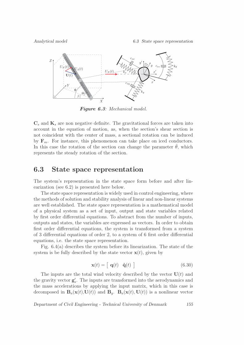
Analytical model 6.3 State space representation
Figure 6.3: Mechanical model.
Cs and Ks are non negative definite. The gravitational forces are taken intoaccount in the equation of motion, as, when the section’s shear section isnot coincident with the center of mass, a sectional rotation can be inducedby Fm. For instance, this phenomenon can take place on iced conductors.In this case the rotation of the section can change the parameter θ, whichrepresents the steady rotation of the section.
6.3 State space representation
The system’s representation in the state space form before and after lin-earization (see 6.2) is presented here below.
The state space representation is widely used in control engineering, wherethe methods of solution and stability analysis of linear and non-linear systemsare well established. The state space representation is a mathematical modelof a physical system as a set of input, output and state variables relatedby first order differential equations. To abstract from the number of inputs,outputs and states, the variables are expressed as vectors. In order to obtainfirst order differential equations, the system is transformed from a systemof 3 differential equations of order 2, to a system of 6 first order differentialequations, i.e. the state space representation.
Fig. 6.4(a) describes the system before its linearization. The state of thesystem is be fully described by the state vector x(t), given by
x(t) =[q(t) q(t)
](6.30)
The inputs are the total wind velocity described by the vector U(t) andthe gravity vector g′
s. The inputs are transformed into the aerodynamics andthe mass accelerations by applying the input matrix, which in this case isdecomposed in Ba(x(t),U(t)) and Bg. Ba(x(t),U(t)) is a nonlinear vector
Department of Civil Engineering - Technical University of Denmark 155

6.3 State space representation Analytical model
which depends on the state parameters x(t) and on the instantaneous windspeed vector U(t):
Ba(x(t),U(t)) = M−1s
[0
Fa(q(t), θ(t),U(t))
](6.31)
where Fa(q(t), θ(t),U(t)) is derived from eq. 6.21 . Bg is equal to the identitymatrix I. The mechanical properties of the structure are assumed to be linearand time invariant.
If the dynamical system is linear and time invariant, the differential andalgebraic equations may be written in matrix form. The study of the motionof the system about the equilibrium points and the study of the stabilityfor small amplitude vibrations is undertaken by a linearization of the systemabout its equilibrium the equilibrium points which are described by
x(t) = 0 (6.32)
The equilibrium points are evaluated considering the non linear system.Fig. 6.4(b) describes the system after linearization. The linearization is de-scribed in paragraph 6.2.3. In this case, the system’s input is representedby the gravity vector g′
s, the mean wind vector U, and by the turbulencevector U(t). The two latter can be summed in one vector which repre-sents the instantaneous wind speed U(t), see eq. 6.1. After linearizationFa(q(t), θ(t),U(t)) is decomposed into four components (eq. 6.22). The firstone is a constant term which depends on U. This term is given by the prod-uct of the input matrix The second and third terms depend on the structuralvelocities and displacements, x(t), respectively and are referred to as self-excited or aeroelastic terms. These terms are given by the product of thematrix Aa times the state vector x(t). From a state space description theaeroelastic term Aa can be considered as a feedback state term that can besummed to the state structural matrix As. The state matrix, As + Aa istime invariant for a given mean wind velocity. The so obtained system isLTI, i.e. linear time invariant.
The state space representation consists of two systems of equations, i.e.
156 Department of Civil Engineering - Technical University of Denmark

Analytical model 6.3 State space representation
(a)
(b)
Figure 6.4: System description pre (a) and after linearization (b)
the state and output system. The state equation is:
x(t) = (As +Aa)x(t) +BsU +BbU(t) +Bgg′s[
q(t)q(t)
]=
[0 I
−M−1s Ks −M−1
s Cs
] [q(t)q(t)
]+
+
[0 0
M−1s ∇q(t)Fa
∣∣(0,0,U)
M−1s ∇q(t)Fa
∣∣(0,0,U)
] [q(t)q(t)
]+
+
[0
M−1s Fa|(0,0,U) U
−1
]U +
[0
M−1s ∇U(t)Fa
∣∣(0,0,U)
]U(t)
+
[0I
]g′s
(6.33)
Department of Civil Engineering - Technical University of Denmark 157

6.4 Eigenvalue problem and instability analysis Analytical model
The output equation, giving the displacement, is:
y(t) = cx(t) + dU =[I 0
] [ q(t)q(t)
](6.34)
The general solution of the problem is:
y(t) = ce(As+Aa)tx(0) +
t∫0
ce(As+Aa)(t−τ)[BsU +BbU(τ) +Bgg
′s
]dτ
= Φ(t)x(0) +
t∫0
ce(As+Aa)(t−τ)[BsU +BbU(τ) +Bgg
′s
]dτ
(6.35)As in the classical solution method for ordinary differential equations with
constant coefficients, the total system state response x(t) is considered assummation of two parts, a homogeneous solution, Φ(t)x(0), which describesthe response of the system to an arbitrary set of initial conditions x(0),and a particular solution which satisfies the state equations for the giveninput. The two components are then combined to form the total response.Φ(t) = e(As+Aa)t is defined to be the state transition matrix.
In state-space terminology, a system is said to be asymptotically stable ifthe homogeneous response of the state vector x(t) returns to the origin of thestate-space from any arbitrary set of initial conditions x(0) as time t → ∞.This definition of stability is equivalent to stating that the homogeneousresponse of all state variables must decay to zero in the absence of any inputto the system, or:
limt→∞
Φ(t)x(0) = 0 (6.36)
A linear system, described by state equations x(t) = Ax(t) + BU , isasymptotically stable if and only if all eigenvalues of the matrix A havenegative real parts. In the next paragraph the solution of the eigenvalueproblem and the determination of the condition of the linear instability willbe analyzed.
6.4 Eigenvalue problem and instability anal-
ysis
In order to find the find the eigenvalues, the characteristic equation is solved:
det([As +Aa]− λ [I]) = 0 (6.37)
158 Department of Civil Engineering - Technical University of Denmark
Analytical model 6.4 Eigenvalue problem and instability analysis
where [As +Aa] is the state-space matrix and [I] is the identity matrix.Equation 6.37 can be reduced to a monic polinomial of order 6, of the form
p(λ) = p0λ6 + p1λ
5 + p2λ4 + p3λ
3 + p4λ2 + p5λ+ p6 = 0 (6.38)
where p0 = 1, and p1-p6 are reported in the Appendix A.5. The problem’seigenvalues are either real values or complex conjugate pairs. The systemis stable if the real parts of all eigenvalues are negative. The characteris-tic equation governing this specific eigenvalue problem is of 6th degree. TheAbel-Ruffini theorem states that there is no general algebraic solution topolynomial equations of 5th degree or higher degree. In these cases, theeigenvalue problem is normally solved numerically. This in order to find thevalue of the structural damping/stiffness at the boundary of instability. Onthe other hand, the Routh-Hurwitz criterion (Hurwitz, 1895) allows to checkthe stability of the system without solving the characteristic equation. Thecriterion establishes that the system is stable, i.e. all roots of the characteris-tic polinomium have negative real parts, if and only if all the leading principalminors of the Hurwitz matrix H, i.e. the so called Hurwitz determinants, arepositive. The Hurwitz matrix is given by
H =
⎡⎢⎢⎢⎢⎢⎢⎣
p1 1 0 0 0 0p3 p2 p1 1 0 0p5 p4 p3 p2 p1 10 p6 p5 p4 p3 p20 0 0 p6 p5 p40 0 0 0 0 p6
⎤⎥⎥⎥⎥⎥⎥⎦ (6.39)
The principal diagonal minors of the Hurwitz matrix are
Δ1 = p1 (6.40)
Δ2 = p1p2 − p3 (6.41)
Δ3 = −p4p21 + p2p3p1 + p5p1 − p23 (6.42)
Δ4 = −p24p21 + p2p6p
21 + p2p3p4p1 − p22p5p1 + 2p4p5p1 − p3p6p1 − p25 − p23p4 + p2p3p5
(6.43)Δ5 = −p26p
31 − p24p5p
21 + p3p4p6p
21 + 2p2p5p6p
21 − p22p
25p1 + 2p4p
25p1 + p2p3p4p5p1+
− p2p23p6p1 − 3p3p5p6p1 − p35 + p2p3p
25 − p23p4p5 + p33p6
(6.44)Δ6 = p6Δ5 (6.45)
As Δ6 = p6Δ5, the stability condition on Δ6 = p6Δ5 reduces to imposingp6 > 0
Department of Civil Engineering - Technical University of Denmark 159

6.5 Application of the 3 DOF model Analytical model
If the 5 principal minors of the Hurwitz matrix, i.e. Δ1 −Δ5 are positiveand the 6th order minor is zero, i.e. Δ6 = 0, the system is at the boundaryof stability. Since Δ6 = p6Δ5, then there are two options:
• the coefficient p6 = 0; this corresponds to the case when one of the rootsof the characteristic equation is zero; the system is on the boundary ofthe aperiodic stability;
• the determinant Δ5 = 0; in this case, there two complex conjugateroots and the system is on the boundary of the oscillatory stability.
In order to simplify the computational problem of the stability analysis,the Lienard-Chipart criterion is here used (Lienard and Chipart, 1914). Thecriterion has the advange of providing a test for the system instability bymeans of a lower number of determinants to be computed. According to thecriterion the system is stable if:
p2, p4, p6 > 0 and Δ1 = p1, Δ3, Δ5 > 0 (6.46)
Note that asp6 = ω2
xω2y
(−ω2aθθ + ω2
θ
)(6.47)
its sign is associated with the occurrence of static divergence-type instability,which occurs when ωaθθ becomes larger than ωθ. The sign of the remainingterms in eq. 6.46 is instead associated with the occurrence of galloping-typeinstabilities.
6.5 Application of the 3 DOF model
The 3-DOF instability model allows to verify the stability of a system againstgalloping and static divergence, to design the minimum structural dampingand stiffness in order to avoid the occurrence of such instabilities, and toderive the trajectories of the motion.
The stability of the system can be verified once its geometrical and struc-tural properties are assigned, i.e. the cable diameter, D, the mass per unitlength, m, the rotational inertia in relation to the mass centre of the cable, J ,the angle offset and distance of the mass center to the shear center of the ca-ble section, ς0 and Le, as well as the vibration frequencies fx′ , fy′ , fθ, and thedamping ratios ξx′ , ξy′ , ξθ′ in the x′, y′, and θ directions. The aerodynamicproperties of the prism, i.e. in terms of drag, lift and moment coefficients forvarying Re, α, Φ, as well as the angle between the wind direction and theprism’s axis, Φ, must also be specified. The stability is verified by applyingthe Lienard-Chipart criterion as illustrated in paragraph 6.4.
160 Department of Civil Engineering - Technical University of Denmark

Analytical model 6.5 Application of the 3 DOF model
In the following, an example of application of the 3-DOF instability modelis proposed. The aerodynamic data, i.e. the quasi-steady drag, lift andmoment, refer to a a series of wind tunnel tests undertaken by Chabartand Lilien (1998) for an iced cable conductor. These are reported in Figs.6.6-6.8. The conductor (see Fig. 6.5) was oriented perpendicular to thewind flow, so that Φ = 90◦. The coefficients were found as independent ofthe Reynolds number for the tested angles-of-attack. Chabart and Lilien(1998) later suspended the same conductor in a wind tunnel with a systemof springs, in order to obtain a system as close as possible to an overheadline, where the vertical, horizontal and rotational movements are allowed.In table 6.1 are summarised the structural and aerodynamic parameters forthe iced cable tested by Chabart and Lilien (1998). As the quasi-steadyforce coefficients were obtained in smooth flow conditions, all unsteady termsaffecting the stability were set equal to zero in the present model. Samedata were employed by Gjelstrup and Georgakis (2011) as an example ofapplication of the 3 DOF model.
Parameter Valuem [kg] 2.99D [m] 0.0325
J [kg/m2] 4.9689e-4Le [m] 0.0025ς0 [◦] 0Φ [◦] 90
fx [Hz] 0.995fy [Hz] 0.845fθ [Hz] 0.865ξx [%] 0.08ξy [%] 0.08ξθ [%] 0.3
Table 6.1: Parameters of the iced conductor employed in the passive-dynamic tests performed by Chabart and Lilien (1998).
In Fig. 6.10(a)-6.10(b) the maps of galloping and static divergence insta-bility obtained by implementing the Lienard-Chiepard criterion are shown.In Fig. 6.10(a) the red colored areas represent the regions where the condition
p2, p4 and Δ1 = p1, Δ3, Δ5 > 0 (6.48)
is satisfied, thus they system in stable against galloping. The blue areasrepresent the regions where at least one of the terms in eq. 6.48 becomes
Department of Civil Engineering - Technical University of Denmark 161

6.5 Application of the 3 DOF model Analytical model
Figure 6.5: Ice shape and aerodynamic forces convention, (Chabart andLilien, 1998).
Figure 6.6: Drag coefficient for varying angles-of-attack, (Chabart andLilien, 1998).
Figure 6.7: Lift coefficient for varying angles-of-attack, (Chabart andLilien, 1998).
negative, thus the system becomes unstable against galloping. In Fig. 6.10(b)
162 Department of Civil Engineering - Technical University of Denmark

Analytical model 6.5 Application of the 3 DOF model
Figure 6.8: Moment coefficient for varying angles-of-attack, (Chabart andLilien, 1998).
the red areas represent the regions where the condition
p6 > 0 (6.49)
is satisfied, thus the system is stable against static divergence instability. Theblue areas are instead associated with negative sign of p6 and thus to staticdivergence-type instability. It is observed that the angle-of-attack regionof galloping instability ranges from 12◦-150◦. On the other hand, staticdivergence instability occurs for angles-of-attack in the range of 25◦-40◦ and60◦-130◦.
Fig. 6.9 shows the regions of instability, i.e. in terms of angle-of-attack,obtained by comparing results of the dynamic tests performed by Chabartand Lilien (1998) (see Test), with the 1 DOF Den Hartog criterion (DenHartog, 1956) (see 1 DOF ), the 2 DOF and 3 DOF instability models derivedby Macdonald and Larose (2008a), and Gjelstrup and Georgakis (2011), (see2 DOF and 3 DOF ). The figure was reported by Gjelstrup and Georgakis(2011). The region of instability obtained from the dynamic tests performedby Chabart and Lilien (1998) spans in the range of 20◦-180◦ angle-of-attack.It is observed that the 3 DOF criterion developed by Gjelstrup and Georgakis(2011) gives a better prediction in comparison to the 1 DOF and 2 DOFcriteria. On the other hand, the present 3 DOF criterion gives an improvedprediction in comparison to Gjelstrup and Georgakis (2011) of the regions ofinstability.
Department of Civil Engineering - Technical University of Denmark 163

6.6 Conclusion Analytical model
Figure 6.9: Regions of instability obtained by comparing experimental re-sults of dynamic tests performed by Chabart and Lilien (1998), with the 1DOF Den Hartog criterion (Den Hartog, 1956), the 2 DOF and 3 DOF in-stability models derived by Macdonald and Larose (2008a), and Gjelstrup andGeorgakis (2011).
(a) (b)
Figure 6.10: Maps of galloping (a) and static divergence (b) instability; blueareas represent the regions of predicted galloping (a) and static divergence (b)instability.
6.6 Conclusion
A new generalized quasi-steady three-degrees-of-freedom analytical model,capable of predicting the aerodynamic instability of a prismatic body withgeneric cross section, and arbitrary orientation with respect to the flow,was here developed. The novelty of the model is the ability to predic twodifferent types of instabilities which can potentially affect the prism, i.e.galloping-type instability associated with the occurrence of negative aerody-namic damping and static divergence type associated with negative aerody-namic stiffness. The model includes finally effects of unsteadiness of the windfield.
164 Department of Civil Engineering - Technical University of Denmark

Analytical model 6.6 Conclusion
An practical implementation to a set of existing wind tunnel data ob-tained for an iced conductor, reveals that the current model gives the bestprediction of the regions of aerodynamic instability, when compared to ex-isting models.
Department of Civil Engineering - Technical University of Denmark 165

6.6 Conclusion Analytical model
166 Department of Civil Engineering - Technical University of Denmark
Bibliography
Blevins, R.D., Iwan, W.D., 1975. The galloping response of a two-degree-of-freedom system. Page 1975 of: American Society of Mechanical Engineers,Applied Mechanics Western Conference, University of Hawaii, Honolulu,Hawaii.
Blevins, R.D., 1977. Flow-induced vibration. New York, Van Nostrand Rein-hold Co., 377,1.
Carassale, L., Freda, A., Piccardo, G., 2004. Quasi-static model for aerody-namic instability of yawed circular cylinder. In: 5th International Collo-quium Bluff Body Aerodynamics and Applications, pp. 401-404.
Carassale, L., Kareem, A., 2010. Modeling nonlinear systems by Volterraseries. Journal of Engineering Mechanics, 136 (6), 801-818.
Chabart, O., Lilien J.L., 1998. Galloping of electrical lines in wind tunnelfacilities. J. Wind Eng. Ind. Aerodyn. 74-76, 967-976.
Cheng, S., Larose G.L., Savage, M., Tanaka, H., Irwin, P.A., 2008a. Experi-mental study on the wind-induced vibration of a dry inclined cable - PartI: Phenomena. J. Wind Eng. Ind. Aerodyn. 96 (12), 2231-2253.
Cheng, S., Irwin P.A., Tanaka, H., 2008b. Experimental study on the wind-induced vibration of a dry inclined cable - Part II: Proposed mechanisms.J. Wind Eng. Ind. Aerodyn. 96 (12), 2254-2272.
Davenport, A.G., Novak, M., 2002. Vibrations of structures induced by fuidflow. In: Chap. 29-II of Harris’ shock and vibration handbook. McGraw-Hill.
Den Hartog, J.P., 1956. Mechanical vibrations. Courier Dover Publications.
Denoel, V., Degee, H. 2006., 1956. Influence of the non-linearity of the aero-dynamic coefficients on the skewness of the buffeting drag force. Wind andStructures, 9, 457-471.
167

BIBLIOGRAPHY BIBLIOGRAPHY
Gjelstrup, H., Georgakis, C.T., 2011. A quasi-steady 3 degree-of-freedommodel for the determination of the onset of bluff body galloping instability.In: Journal of Fluids and Structures, 27 (7), 1021-1034.
Gjelstrup, H., Georgakis, C.T., 2011. A quasi-steady 3 degree-of-freedommodel for the determination of the onset of bluff body galloping instability.In: Journal of Fluids and Structures, 27 (7), 1021-1034.
Hurwitz, A., 1895. Ueber die Bedingungen, unter welchen eien Gleichung nurWurzeln mit negativen reellen Theilen besitzt. Mathematische Annalen,46, 273-284.
Jones, K., 1992. Coupled vertical and horizontal galloping. Journal of Engi-neering Mechanics, 118 (1), 92-107.
Kareem, A., Wu, T., 2013. Wind-induced effects on bluff bodies in turbu-lent flows: Nonstationary, non-Gaussian and nonlinear features. Journalof Wind Engineering and Industrial Aerodynamics, 122, 21-37.
Lienard, A., Chipart, M.H., 1914. Sur le signe de la partie reelle des racinesdune equation algebrique. J. Math. Pure Appl, 10 (4), 291-346.
Luongo, A., Piccardo, G., 2005. Linear instability mechanisms for coupledtranslational galloping. J. of Sound and Vibration, 288, 1027-1047.
Macdonald, J.HJ., Larose G.L., 2008a. A unified approach to aerodynamicdamping and drag/lift instabilities, and its application to dry inclined cablegalloping. J. Fluids Struct. 22, 229-252.
Macdonald, J.HJ., Larose G.L., 2008a. Two-degree-of-freedom inclined gal-loping - Part 1: general formulation and solution for perfectly tuned sys-tem. J. Wind Eng. Ind. Aerodyn., 96 (3), 291-307.
Macdonald, J.HJ., Larose G.L., 2008a. Two-degree-of-freedom inclined gal-loping - Part 2: analysis and prevention for an arbitrary frequency ratio.J. Wind Eng. Ind. Aerodyn., 96 (3), 308-326.
Martin, W.W., Currie, I.G., Naudascher, E., 1981. Streamwise oscillations ofcylinders. Journal of the Engineering Mechanics Division-ASCE 107 (3),589-607.
Nakamura, Y., Mizota, T., 1975. Torsional flutter of rectangular prisms.Journal of the Engineering Mechanics Division-ASCE. (NEM2), 125-142.
168 Department of Civil Engineering - Technical University of Denmark

BIBLIOGRAPHY BIBLIOGRAPHY
Nigol, O., Buchan, P.G., 1981b. Conductor galloping-part II Torsional Mech-anism. Power Apparatus and Systems, IEEE Transactions on, 708-720.
Raeesi, A., Cheng, S., Ting, D. S-K. 2013. Aerodynamic damping of an in-clined circular cylinder in unsteady flow and its application to the predic-tion of dry inclined galloping. Journal of Wind Engineering and IndustrialAerodynamics, 113, 12-28.
Symes, J.A., Macdonald, J.H.G., 2006. Quasi-steady dry-galloping analysisof inclined cables in turbulent flow. Pages 121-124 of: Proceedings of 7thUK Conference on Wind Engineering, Glasgow.
Symes, J.A., Macdonald, J.H.G., 2007. Combined buffeting and dry gallop-ing analysis of inclined stay-cables. Pages 201-208 of: 7th InternationalSymposium on Cable Dynamics, Vienna.
Stoyanoff, S., 2001. A unified approach for 3D stability and time domainresponse analysis with application of quasi-steady theory. J. Wind Eng.Ind. Aerodyn., 89 (14), 1591-1606.
Yu, P., Shah, A.H., Popplewell, N., 1992. Inertially coupled galloping of icedconductors. J. of Applied Mechanics, 59, 140.
Yu, P., Desai, Y.M., Shah, A.H., Popplewell, N., 1993. Three-degree-of-freedom model for galloping. Part I: Formulation. J. of Engineering Me-chanics, 119 (12), 2404-2425.
Department of Civil Engineering - Technical University of Denmark 169

BIBLIOGRAPHY BIBLIOGRAPHY
170 Department of Civil Engineering - Technical University of Denmark

Chapter 7
Conclusions
In the present thesis the mechanisms of vibration of bridge cables undervarying meteorological conditions have been investigated by following a twinresearch approach, i.e. climatic wind tunnel testing of full-scale bridge cablesections and theoretical modelling.
Bridge cables are classified as bluff bodies and as such can only undergoinstabilities of vortex shedding-, buffeting- and galloping-type. A literaturereview on the possible excitation mechanisms of inclined bridge cables underdifferent climatic conditions, i.e. dry, wet and iced, was first undertaken.The study helped to systematize the current knowledge of the associatedexcitation mechanisms, based on results of full-scale monitoring, wind tunneltesting and theoretical modelling. Several aspects of the instability needingmore clarification were identified, so to inspire the wind tunnel test campaignprogramme and the theoretical modelling.
Static wind tunnel tests were first undertaken on full-scale plain surfacedbridge cable section models, oriented perpendicular or inclined/yawed to theflow, in dry conditions. Tests were undertaken for varying Reynolds num-bers, cable-wind angles, angles-of-attack and turbulence intensities. It wasobserved that the cable’s drag coefficient is fairly consistent with angle-of-attack, while the lift coefficient changes significantly, given all other parame-ters fixed. These changes can be triggered by small geometrical imperfectionsof the cable model, such as surface roughness alterations or distortions ofthe shape. Assuming the validity of the quasi-steady theory, negative aero-dynamic damping can be predicted in the critical Reynolds number rangewhere the drag coefficient is reduced to its minimum and the lift coefficientexperiences significant variations in sign and amplitude with angle-of-attack.Although important for theoretical modeling and section model testing, vari-ations in the drag and lift coefficients with angle-of-attack may not ultimatelybe important when averaged over the full length of an inclined structural ca-
171

Conclusions
ble.Passive-dynamic wind tunnel tests were later undertaken for a dry plain
surfaced cable section model of the same type as the one tested in staticconditions. Tests were undertaken at a critical cable-wind angle for the oc-currence of dry inclined galloping, which had equally been been tested usingthe static setup. The cable’s mass and frequency were fixed. Results showedthat the aerodynamic damping as well as the peak to peak amplitude changesignificantly with Reynolds number, for varying degrees of axial rotation ofthe cable model, i.e. angles-of-attack. In particular, minor deviations in thecable response are observed in the subcritical Reynolds number range. Onthe other hand, in the critical Reynolds number range the cable can eitherexhibit a stable response, characterised by positive aerodynamic dampingand limited peak to peak amplitudes of vibration, or can undergo divergentvibration accompanied by negative aerodynamic damping. Thus, dry insta-bility is very sensitive to microscopic geometrical imperfections of the cablemodel and can occur over a large range of Reynolds numbers. This confirmsexperimental findings of the static tests.
Passive-dynamic wind tunnel tests were later undertaken for an inclinedand yawed plain surfaced full-scale plain bridge cable model in rainy cond-tions. Tests were performed for varying levels of the mass and wettabilityof the cable and helped to better understand the rain-wind induced and dryinstabilities. In particular, galloping-type instability was detected in dry con-ditions in the critical Reynolds number range. Under the effects of wind andrain, the cable model underwent different types of instability mechanisms,depending on the level of surface wettability and of mass. RWIV instabilitywas observed only when the cable surface was characterised by an increasedlevel of wettability, for all tested mass levels. The instability occurred onlyfor a limited range of Reynolds number and as in the dry state was againcharacterized by the occurrence of large amplitude vibrations accompaniedby negative aerodynamic damping. No RWIV instability was experienced forthe cable model with very low wettability, either in presence of steady waterrivulets, induced by a uniform water flow, or in presence of droplets, in thedrying state.
In order to complement the understanding achieved by wind tunnel ex-periments, a new generalized quasi-steady three-degrees-of-freedom analyti-cal model, capable of predicting the aerodynamic instability of a prismaticbody with generic cross section, and arbitrary orientation with respect to theflow, was finally developed. The novelty of the model is the ability to predictwo different types of instabilities which can potentially affect the prism,i.e. galloping instability associated with the occurrence of negative aerody-namic damping and torsional divergence, associated with negative aerody-
172 Department of Civil Engineering - Technical University of Denmark

Conclusions
namic stiffness. Effects of unsteadiness of the wind field were included in themodel. Note also that the time dependency of the prism’s cross section wasneglected. Thus, the current model applies only to the dry and iced state,but not to the wet state. In fact, even though the ice accretion provokes atemporal change of cable’s cross section, the time scale of such variation ismuch slower than other aerodynamic phenomena which might be responsiblefor the instantaneous instability. On the other hand, in rainy conditions,the time fluctuations of the cross-sectional shape are much faster and needto be accounted for in the mathematical modelling of the associated excita-tion. A practical implementation of the present model to a set of existingwind tunnel data obtained for an iced conductor, revealed that it gives thebest prediction of the regions of aerodynamic instability, when compared toexisting criteria.
7.0.1 Future work
Understanding of bridge vibrations under varying meteorological conditions isa very wide and complex topic of research. It is fair to state that after manyyears of experimental and theoretical research bridge cable instabilities arestill not completely predictable. Investigations performed within this disser-tation have attempted to understand and explain part of the vibration issues.Nevertheless numerous topics of potential investigation exist. A selection ofthese is here suggested.
Effects of roughness/shape deviations of the HPDE sheat on theforce coefficients at varying levels of turbulence intensity
In the present study the dependency of the force coefficients of inclined cableson Reynolds number and angle-of-attack has been presented only for smoothflow conditions, i.e. at turbulence intensity below 1%. It was demonstratedthat the lift coefficients is significantly affected by changes in the angle-of-attack, due to the non uniform shape/roughness of the cable model. It isinteresting to understand whether this effect is evident at larger turbulenceintensities, which are likely to occur on bridges. Additional tests should becarried out, at increased levels of wind tunnel along-cable axis turbulence in-tensity. Tests should be performed for varying orientations of the cable axiswith respect to the wind direction and angles-of-attack. The so obtainedaerodynamic data might as well be useful for design purposes. The drag, liftand moment coefficients should then be implemented in the quasi-steady an-alytical model developed within this dissertation, in order to predict regionsof aerodynamic instability. For verification, passive-dynamic studies should
Department of Civil Engineering - Technical University of Denmark 173

Conclusions
also be performed at the same level of turbulence intenstity and for the samegeometrical attitudes of the cable model.
Investigation of vortex induced vibration at high reduced velocityand dry inclined galloping by means of static and passive-dynamicwind tunnel tests
Passive-dynamic wind tunnel tests have shown that stay cables may eitherundergo divergent motion, i.e. dry galloping, or limited amplitude motionunder a limited interval of wind speed, i.e. vortex induced vibration at highreduced wind velocities. It is still not yet clear whether the two forms ofinstability can only occur under a specific combination of parameters suchas geometrical orientation of the cable model to the wind flow, wind veloc-ity, surface roughness, mass and frequency, or they are interconnected, sothat one form of instability could evolve into the other. Additional passive-dynamic wind tunnel tests should be performed in order to better under-stand and characterise these two forms of instability. Static wind tunneltests should also be undertaken, for cable models charactersed by the samesurface properties, orientations to the wind flow, and end conditions. Forcompleteness smoke visualization tests could be performed in order to un-derstand the features of the flow in the cable’s wake, for example the axialflow, which is believed to play a crucial role in the dry inclined excitation.
Angle-of-attack dependency of the force coefficients of inclined/yawedcable models in the iced state
Numerous experimental and theoretical studies have demonstrated that forinclined cables, especially when characterised by a generic cross-sectionalshape, as in the iced state, the combination of three parameters affects thetrend of the force coefficients and the associated aerodynamic instabilities,i.e the Reynolds number, the angle between the cable axis and the winddirection, and the angle-of-attack.
Static tests have been performed at the DTU/Force climatic wind tun-nel in iced conditions for horizontal and vertical cable models for varyingReynolds number and angles-of-attack. Aerodynamic force coefficients havebeen implemented in the 1 DOF Den Hartog instability criterion in order topredict the regions where galloping vibrations could potentially occur. Staticwind tunnel tests have been performed additionally for inclined/yawed ca-ble models in the iced state. In this case the focus of the investigation wasthe dependency of the force coefficients on the angle between the cable axisand the wind direction, leaving out the dependency on the angle-of-attack.
174 Department of Civil Engineering - Technical University of Denmark

Conclusions
Additional wind tunnel tests should be performed where the combinationof all three parameters (i.e Reynolds number, cable-wind angle, and angle-of-attack) on the aerodynamic force coefficients is investigated. The aero-dynamic data should be implemented in the quasi-steady analytical modeldeveloped within this dissertation in order to predict the regions of instabil-ity.
Passive-dynamic wind tunnel testing of cable sections in iced state
Passive-dynamic wind tunnel tests should be performed for horizontal/verticaland inclined/yawed bridge cables, in iced conditions. It is recognised that atpresent moment the characteristics of this iced cable instability are unknow,as no wind tunnel dynamic or full scale monitoring investigation have beenperformed. This implies that a very large parametric study should be under-taken, where the combination of numerous parameters should be investigatedsuch as range of critical cable-wind angles, Reynolds number, angle-of-attack.Moreover, attention should be payed the role on the instability of cable mass,frequency and structural damping. Data from passive-dynamic tests couldbe useful for validating predictions of aerodynamic instability based on ap-plication of quasi-steady aerodynamic criteria.
Investigation of the aerodynamic instability of a streamlined body
The analytical model derived within this dissertation applies for a prismwith generic cross-section, i.e. either bluff or streamlined. It could be ofinterest to attempt an application of the model to a streamlined body, whichis expected to exhibit a completely different aerodynamic behaviour froma bridge cable. Static and passive-dynamic tests should be performed, soimplement the quasi-steady aerodynamic coefficients in the model, and tocompare the regions of aerodynamic instability determined analytically withexperimental (dynamic) predictions.
Elimination of the quasi-steady steady assumption in the 3 DOFanalytical model
The analytical model derived within this dissertation could be extended inorder to predict unsteady aerodynamic phenomena such as flutter. Thisrequires a reformulation of the aerodynamic damping and stiffness matrices,i.e. as in terms of flutter derivatives.
Department of Civil Engineering - Technical University of Denmark 175
Conclusions
176 Department of Civil Engineering - Technical University of Denmark

Appendix A
Analytical model
A.1 Derivation of the aerodynamic forces
In the following, detailed derivation of the linearized expression of the aero-dynamic forces, based on equation 6.22, is reported. Generally, the gradientof the aerodynamic force per unit length Fa(q(t), θ(t),U(t)) with respect toa generic vector time function f(t) can be written as
∇f(t)Fa
∣∣(0,0,U)
=ρν2
2D
{[(Rz(αR)C)⊗ (∇f(t)Re2R
)]+Re2R
[(∇f(t)Rz(αR)C)+
+Rz(αR)(∇f(t)C
)]}∣∣(0,0,U)
(A.1)Equation A.1 is made of three main terms which can be further simplified.
In particular:
∇f(t)Re2R = 2ReR∇f(t)ReR = 2ReR∇f(t)T11b1 = 2ReRD
ν∇f(t)UR (A.2)
The second term is a third order tensor obtained from the derivation of therotation matrix with respect to the structural velocity vector. This tensor canbe reduced in the tensorial product of two vectors considering the properties:
∂ cos f(x)
∂x= −∂f(x)
∂xsin x
∂ sin f(x)
∂x=
∂f(x)
∂xcosx (A.3)
that are the term contained in the rotation matrix. After simple manipulationit is obtained:
∇f(t)Rz(αR)C = FC⊗∇f(t)αR (A.4)
where
F = ∇xRz(x)|x=ϕ =
⎡⎣− sin(ϕ) − cos(ϕ) 0cos(ϕ) − sin(ϕ) 0
0 0 0
⎤⎦ (A.5)
177

A.1 Derivation of the aerodynamic forces Analytical model
As the vector of the aerodynamic coefficientsC depends on f(t), where f(t) =q(t), q(t) or U(t), towards d, the chain rule need to be implemented. Thisis given by:
∇q(t)C∣∣(0,0,U)
=[(∇dC)
(∇f(t)d)]∣∣
(0,0,U)(A.6)
Eq. A.1 may thus be re-written as
∇f(t)Fa
∣∣(0,0,U)
=ρν2
2D
{[(Rz(αR)C)⊗
((2Re
D
ν
)∇f(t)UR
)]+Re2R
[(FC⊗∇f(t)αR
)+
+Rz(αR)[(∇dC)
(∇f(t)d)]]}∣∣
(0,0,U)
(A.7)The structural velocity and displacement proportional terms of equation 6.22are obtained by setting f(t) = q(t) and f(t) = q(t) in equation A.1.
The nil-mean fluctuating wind velocity proportional terms, i.e. buffetingterms, are similarly obtained upon substitution of f(t) = U(t) in equationA.1.
178 Department of Civil Engineering - Technical University of Denmark

Analytical model A.2 Flow variables linearization
A.2 Flow variables linearization
The vector b(q(t), θ(t),U(t))
b(q(t), q3(t),U(t)) =
⎡⎣UR(q, θ(t),U(t)))αR(q, θ(t),U(t)))ΦR(q, θ(t),U(t)))
⎤⎦ (A.8)
is equally Taylor expanded as
b(q(t), θ(t),U(t)) = b|(0,0,U) + ∇U(t)b∣∣(0,0,U)
(U(t)−U)+
+ ∇q(t)b∣∣(0,0,U)
q(t) + ∇q(t)b∣∣(0,0,U)
q(t) =
=
⎡⎣UϕΦ
⎤⎦+
+
⎡⎢⎢⎢⎢⎢⎣1 0 0
0sinΘ(1 + tan2 β)
U(sin2 Θ+ tan2 β)
sin β cosΘ
U cos2 β(sin2 Θ+ tan2 β)
0 −cosΘ sin β
U sinΦ
sinΘ
U sinΦ
⎤⎥⎥⎥⎥⎥⎦⎡⎣ u(t)v(t)w(t)
⎤⎦+
+
⎡⎢⎢⎢⎢⎣− cos ϕ sinΦ − sin ϕ sinΦ Rδ sin δ sinΦ
sin ϕ
U sinΦ− cos ϕ
U sinΦ
−Rδ cos δ
U sinΦ
−cos ϕ cosΦ
U−sin ϕ cosΦ
U
Rδ sin δ cosΦ
U
⎤⎥⎥⎥⎥⎦⎡⎣ξ(t)η(t)
θ(t)
⎤⎦
+
⎡⎣0 0 00 0 −10 0 0
⎤⎦⎡⎣ξ(t)η(t)θ(t)
⎤⎦(A.9)
Department of Civil Engineering - Technical University of Denmark 179

A.2 Flow variables linearization Analytical model
The linearized version of d(q(t),q(t)) is obtained:
d(q(t), θ(t),U(t)) = Tb(q(t), θ(t)) =
=[ReR(q, θ(t),U(t))) αR(q, θ(t),U(t))) ΦR(q, θ(t),U(t)))
]T=
=
⎡⎣ReϕΦ
⎤⎦+
+
⎡⎢⎢⎢⎢⎢⎢⎣
D
ν0 0
0D sinΘ(1 + tan2 β)
νRe(sin2 Θ+ tan2 β)
D sin β cosΘ
νRe cos2 β(sin2 Θ+ tan2 β)
0 −D cosΘ sin β
νRe sinΦ
D sinΘ
νRe sinΦ
⎤⎥⎥⎥⎥⎥⎥⎦⎡⎣ u(t)v(t)w(t)
⎤⎦+
+
⎡⎢⎢⎢⎢⎢⎢⎣−D cos ϕ sinΦ
ν−D sin ϕ sinΦ
ν
DRδ sin δ sinΦ
νD sin ϕ
νRe sinΦ− D cos ϕ
νRe sinΦ
−DRδ cos δ
νRe sinΦ
−D cos ϕ cosΦ
νRe−D sin ϕ cosΦ
νRe
DRδ sin δ cosΦ
νRe
⎤⎥⎥⎥⎥⎥⎥⎦⎡⎣ξ(t)η(t)
θ(t)
⎤⎦+
+
⎡⎣0 0 00 0 −10 0 0
⎤⎦⎡⎣ξ(t)η(t)θ(t)
⎤⎦(A.10)
In eq. A.10, U is set equal to Re ν/D.
180 Department of Civil Engineering - Technical University of Denmark

Analytical model A.3 Aerodynamic forces linearization
A.3 Aerodynamic forces linearization
The linearization of the aerodynamic damping matrix is
∇q(t)Fa
∣∣(0,0,U)
=ρν2
2D
{[(Rz(αR)C)⊗
((2Re
D
ν
)∇q(t)UR
)]+Re2R
[(FC⊗∇q(t)αR
)+
+Rz(αR)[(∇dC)
(∇q(t)d)]]}∣∣
(0,0,U)
(A.11)
ρν2
2D(Rz(αR)C)⊗ (2Re
D
ν∇q(t)UR)
∣∣∣∣(0,0,U)
= ρνRe sinΦ
⎡⎣f1 f2 f3f4 f5 f6f7 f8 f9
⎤⎦(A.12)
f1 = − cos ϕ (Cx′ cos ϕ− Cy′ sin ϕ) (A.13)
f2 = − sin ϕ (Cx′ cos ϕ− Cy′ sin ϕ) (A.14)
f3 = Rδ sin δ [Cx′ cos ϕ− Cy′ sin ϕ] (A.15)
f4 = − cos ϕ (Cx′ sin ϕ+ Cy′ cos ϕ) (A.16)
f5 = − sin ϕ (Cx′ sin ϕ+ Cy′ cos ϕ) (A.17)
f6 = Rδ sin δ (Cx′ sin ϕ+ Cy′ cos ϕ) (A.18)
f7 = −DCM cos ϕ (A.19)
f8 = −DCM sin ϕ (A.20)
f9 = DCMRδ sin δ (A.21)
ρν2
2DRe2R(FC⊗∇q(t)αR)
∣∣∣∣(0,0,U)
=ρνRe
2 sinΦ
⎡⎣g1 g2 g3g4 g5 g60 0 0
⎤⎦ (A.22)
g1 = − sin ϕ (Cx′ sin ϕ+ Cy′ cos ϕ) (A.23)
Department of Civil Engineering - Technical University of Denmark 181

A.3 Aerodynamic forces linearization Analytical model
g2 = cos ϕ (Cx′ sin ϕ+ Cy′ cos ϕ) (A.24)
g3 = Rδ cos δ(Cx′ sin ϕ+ Cy′ cos ϕ) (A.25)
g4 = sin ϕ (Cx′ cos ϕ− Cy′ sin ϕ) (A.26)
g5 = − cos ϕ (Cx′ cos ϕ− Cy′ sin ϕ) (A.27)
g6 = −Rδ cos δ (Cx′ cos ϕ− Cy′ sin ϕ) (A.28)
ρν2
2DRe2RRz(αR)
[(∇dC)
(∇q(t)d)]∣∣∣∣
(0,0,U)
=ρνRe
2
⎡⎣h1 h2 h3
h4 h5 h6
h7 h8 h9
⎤⎦ (A.29)
h1 =
[cos ϕ
(sin ϕ
sinΦ
∂Cx′
∂αR
− cos ϕ
(cosΦ
∂Cx′
∂Φ+ sinΦ
∂Cx′
∂ReRe
))+sin ϕ
(− sin ϕ
sinΦ
∂Cy′
∂αR
+ cos ϕ
(cosΦ
∂Cy′
∂Φ+ sinΦ
∂Cy′
∂ReRe
))] (A.30)
h2 =
[cos ϕ
(−cos ϕ
sinΦ
∂Cx′
∂αR
− sin ϕ
(cosΦ
∂Cx′
∂Φ+ sinΦ
∂Cx′
∂ReRe
))+sin ϕ
(cos ϕ
sinΦ
∂Cy′
∂αR
+ sin ϕ
(cosΦ
∂Cy′
∂Φ+ sinΦ
∂Cy′
∂ReRe
))] (A.31)
h3 = Rδ
[cos ϕ
(− cos δ
sinΦ
∂Cx′
∂αR
+ sin δ
(cosΦ
∂Cx′
∂Φ+ sinΦD
∂Cx′
∂ReRe
))+sin ϕ
(cos δ
sinΦ
∂Cy′
∂αR
− sin(δ)
(cosΦ
∂Cy′
∂Φ+ sinΦD
∂Cy′
∂ReRe
))](A.32)
h4 = sin ϕ
[sin ϕ
sinΦ
∂Cx′
∂αR
− cos ϕ
(cosΦ
∂Cx′
∂Φ+ sinΦ
∂Cx′
∂ReRe
)]+ cos ϕ
[sin ϕ
sinΦ
∂Cy′
∂αR
− cos ϕ
(cosΦ
∂Cy′
∂Φ+ sinΦ
∂Cy′
∂ReRe
)] (A.33)
h5 = sin ϕ
[−cos ϕ
sinΦ
∂Cx′
∂αR
− sin ϕ
(cosΦ
∂Cx′
∂Φ+ sinΦ
∂Cx′
∂ReRe
)]+ cos ϕ
[−cos ϕ
sinΦ
∂Cy′
∂αR
− sin ϕ
(cosΦ
∂Cy′
∂Φ+ sinΦ
∂Cy′
∂ReRe
)] (A.34)
h6 = Rδ
[sin ϕ
(− cos δ
sinΦ
∂Cx′
∂αR
+ sin δ
(cosΦ
∂Cx′
∂Φ+ sinΦ
∂Cx′
∂ReRe
))+cos ϕ
(− cos δ
sinΦ
∂Cy′
∂αR
+ sin δ
(cosΦ
∂Cy′
∂Φ+ sinΦ
∂Cy′
∂ReRe
))](A.35)
182 Department of Civil Engineering - Technical University of Denmark

Analytical model A.3 Aerodynamic forces linearization
h7 = D
[sin ϕ
sinΦ
∂CM
∂αR
− cos ϕ
(cosΦ
∂CM
∂Φ+ sinΦ
∂CM
∂ReRe
)](A.36)
h8 = D
[−cos ϕ
sinΦ
∂CM
∂αR
− sin ϕ
(cosΦ
∂CM
∂Φ+ sinΦ
∂CM
∂ReRe
)](A.37)
h9 = DRδ
[− cos δ
sinΦ
∂CM
∂αR
+ sin δ
(cosΦ
∂CM
∂Φ+ sinΦ
∂CM
∂ReRe
)](A.38)
The linearization of the aerodynamic stiffness matrix is
∇q(t)Fa
∣∣(0,0,U)
=ρν2
2D
{[(Rz(αR)C)⊗
((2Re
D
ν
)∇q(t)UR
)]+Re2R
[(FC⊗∇q(t)αR
)+
+Rz(αR)[(∇dC)
(∇q(t)d)]]}∣∣
(0,0,U)
(A.39)ρν2
2D(Rz(αR)C)⊗ (2Re
D
ν∇q(t)UR)
∣∣∣∣(0,0,U)
= 0 (A.40)
ρν2
2DRe2R(FC⊗∇q(t)αR)
∣∣∣∣(0,0,U)
=ρν2
2DRe2
⎡⎢⎣0 0 Cx′ sin ϕ+ Cy′ cos ϕ
0 0 −Cx′ cos ϕ+ Cy′ sin ϕ
0 0 0
⎤⎥⎦(A.41)
ρν2
2DRe2RRz(αR)
[(∇dC)
(∇q(t)d)]∣∣∣∣
(0,0,U)
=ρν2
2DRe2
⎡⎢⎢⎢⎢⎢⎢⎣0 0 −∂Cx′
∂αcos ϕ+
∂Cy′
∂αsin ϕ
0 0 −∂Cx′
∂αsin ϕ− ∂Cy′
∂αcos ϕ
0 0 −D∂CM
∂α
⎤⎥⎥⎥⎥⎥⎥⎦(A.42)
The linearization of the buffeting matrix is
∇U(t)Fa
∣∣(0,0,U)
=ρν2
2D
{[(Rz(αR)C)⊗
((2Re
D
ν
)∇U(t)UR
)]+Re2R
[(FC⊗∇U(t)αR
)+
+Rz(αR)[(∇dC)
(∇U(t)d)]]}∣∣
(0,0,U)
(A.43)
ρν2
2D(Rz(αR)C)⊗ (2Re
D
ν∇U(t)UR)
∣∣∣∣(0,0,U)
= ρνRe
⎡⎣cos ϕCx′ − sin ϕCy′ 0 0sin ϕCx′ + cos ϕCy′ 0 0
DCM 0 0
⎤⎦(A.44)
ρν2
2DRe2R(FC⊗∇U(t)αR)
∣∣∣∣(0,0,U)
=ρνRe
2
⎡⎣0 l1 l20 l3 l40 0 0
⎤⎦ (A.45)
Department of Civil Engineering - Technical University of Denmark 183
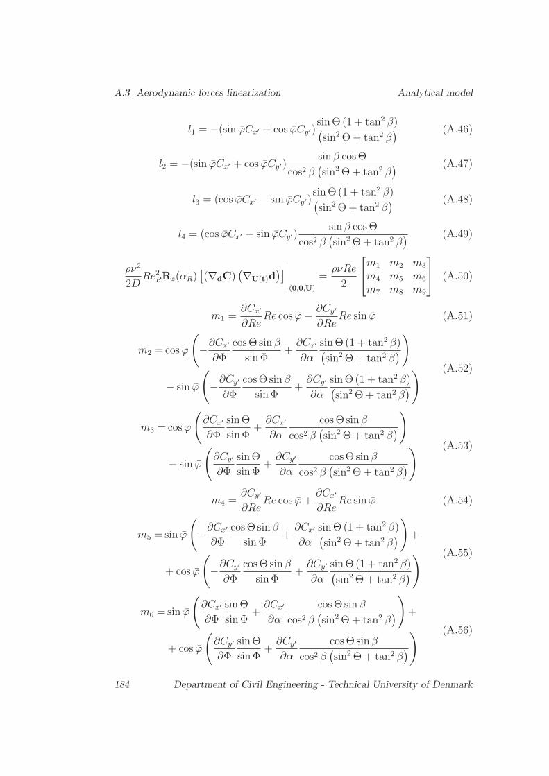
A.3 Aerodynamic forces linearization Analytical model
l1 = −(sin ϕCx′ + cos ϕCy′)sinΘ (1 + tan2 β)(sin2 Θ+ tan2 β
) (A.46)
l2 = −(sin ϕCx′ + cos ϕCy′)sin β cosΘ
cos2 β(sin2 Θ+ tan2 β
) (A.47)
l3 = (cos ϕCx′ − sin ϕCy′)sinΘ (1 + tan2 β)(sin2 Θ+ tan2 β
) (A.48)
l4 = (cos ϕCx′ − sin ϕCy′)sin β cosΘ
cos2 β(sin2 Θ+ tan2 β
) (A.49)
ρν2
2DRe2RRz(αR)
[(∇dC)
(∇U(t)d)]∣∣∣∣
(0,0,U)
=ρνRe
2
⎡⎣m1 m2 m3
m4 m5 m6
m7 m8 m9
⎤⎦ (A.50)
m1 =∂Cx′
∂ReRe cos ϕ− ∂Cy′
∂ReRe sin ϕ (A.51)
m2 =cos ϕ
(−∂Cx′
∂Φ
cosΘ sin β
sinΦ+
∂Cx′
∂α
sinΘ (1 + tan2 β)(sin2 Θ+ tan2 β
))
− sin ϕ
(−∂Cy′
∂Φ
cosΘ sin β
sinΦ+
∂Cy′
∂α
sinΘ (1 + tan2 β)(sin2 Θ+ tan2 β
)) (A.52)
m3 =cos ϕ
(∂Cx′
∂Φ
sinΘ
sinΦ+
∂Cx′
∂α
cosΘ sin β
cos2 β(sin2 Θ+ tan2 β
))
− sin ϕ
(∂Cy′
∂Φ
sinΘ
sinΦ+
∂Cy′
∂α
cosΘ sin β
cos2 β(sin2 Θ+ tan2 β
)) (A.53)
m4 =∂Cy′
∂ReRe cos ϕ+
∂Cx′
∂ReRe sin ϕ (A.54)
m5 =sin ϕ
(−∂Cx′
∂Φ
cosΘ sin β
sinΦ+
∂Cx′
∂α
sinΘ (1 + tan2 β)(sin2 Θ+ tan2 β
))+
+ cos ϕ
(−∂Cy′
∂Φ
cosΘ sin β
sinΦ+
∂Cy′
∂α
sinΘ (1 + tan2 β)(sin2 Θ+ tan2 β
)) (A.55)
m6 =sin ϕ
(∂Cx′
∂Φ
sinΘ
sinΦ+
∂Cx′
∂α
cosΘ sin β
cos2 β(sin2 Θ+ tan2 β
))+
+ cos ϕ
(∂Cy′
∂Φ
sinΘ
sinΦ+
∂Cy′
∂α
cosΘ sin β
cos2 β(sin2 Θ+ tan2 β
)) (A.56)
184 Department of Civil Engineering - Technical University of Denmark

Analytical model A.3 Aerodynamic forces linearization
m7 =D∂CM
∂ReRe (A.57)
m8 = −D∂CM
∂Φ
cosΘ sin β
sinΦ+
D∂CM
∂α
sinΘ (1 + tan2 β)(sin2 Θ+ tan2 β
) (A.58)
m9 =D∂CM
∂Φ
sinΘ
sinΦ+
D∂CM
∂α
cosΘ sin β
cos2 β(sin2 Θ+ tan2 β
) (A.59)
Department of Civil Engineering - Technical University of Denmark 185

A.4 Equations of motion Analytical model
A.4 Equations of motion
Fig. A.1 shows the definition of the mass center coordinates. The centerof mass CM is located at distance Le from the origo of the local body’sreference system (x, y) and at angular distance γ0 from the x axis. Due tomovement of the body along both x and y directions, the the center of massis displaced to CM ′. Due to torsional rotation θ the final position of thecenter of mass is CM ′′.
Figure A.1: Definition of the mass center coordinates.
The rigid rotation and translation of the section about the Shear Center(SC) is evaluated for the Center of Mass (CM) as A.1:
rg(t) = q(t) + ω(t) ∧ L0 (A.60)
The kinetic energy is evaluated as:
T =1
2
(∣∣Ir2g(t)∣∣) (A.61)
The potential energy is evaluated as:
V =1
2
(∣∣Ksr2g(t)
∣∣) (A.62)
The dissipative terms are:
FD = Csq(t) (A.63)
186 Department of Civil Engineering - Technical University of Denmark

Analytical model A.4 Equations of motion
where:
I =
⎡⎣ m 0 00 m 00 0 J
⎤⎦ (A.64)
Cs =
⎡⎣ csx 0 00 csy 00 0 csz
⎤⎦ = 2
⎡⎣ mξxωx 0 00 mξyωy 00 0 Jξθωθ
⎤⎦ (A.65)
Ks =
⎡⎣ ksx 0 00 ksy 00 0 ksθ
⎤⎦ =
⎡⎣ mω2x 0 0
0 mω2y 00
0 0 Jω2θ
⎤⎦ (A.66)
The equation of motion:
∇t
(∇q(t)(T − V ))−∇q(t)(T − V ) + FD = Fm + Fa (A.67)
The final result of the EOM is:
Msq(t) +Csq(t) +Ksq(t) = Fm + Fa (A.68)
where:
Ms =
⎡⎣ m 0 −mL0 sin ς00 m mL0 cos ς0
−mL0 sin ς0 mL0 cos ς0 J +mL20
⎤⎦ (A.69)
Department of Civil Engineering - Technical University of Denmark 187

A.5 Terms of the characteristic polynomium Analytical model
A.5 Terms of the characteristic polynomium
p0 = 1 (A.70)
p1 = ξxωx
(2 +
2m sin ς20ωxL2e
J
)+ ξyωy
(2 +
2m cos ς20L2e
J
)+ 2ξθωθ+
+ ωx
(−2ξaxx +
2mLe
J
(−Le sin ς20ξaxx + sin(2ς0)Leξaxy − sin ς0ξaxθ
))+
+ ωy
(−2ξayy +
2mLe
J
(cos ς0 sin ς0Leξayx − cos ς20Leξayy + cos ς0ξayθ
))+
+ ωθ (−2ξaθθ + 2Le (− sin ς0ξaθx + cos ς0ξaθy))(A.71)
p2 = ξxωx
((−4ξayy +
4mLe
J(−Leξayy + cos ς0ξayθ)
)ωy
)+
+ ξxωx (4 cos ς0Leξaθy − 4ξaθθ)ωθ+
+ ξy
((−4ξaxx − 4mLe
J(Leξaxx + sin ς0ξaxθ)
)ωxωy
)+
− ξy (4 sin ς0Leξaθx + 4ξaθθ)ωyωθ+
− ξθ (4ξaxxωx + 4ξayyωy)ωθ + ξxξy
(4 +
4mL2e
J
)ωxωy + 4ξxξθωxωθ+
+ 4ξyξθωyωθ +
(1 +
m sin ς20L2e
J
)ω2x +
(1 +
m cos ς20L2e
J
)ω2y + ω2
θ+
+ (ξayy (4 sin ς0Leξaθx + 4ξaθθ)− ξaθy (4 sin ς0Leξayx + ξayθ))ωyωθ+
+ ωx
((4 (ξaxxξayy − ξaxyξayx) +
4mLe
J
(ξaxx (Leξayy − cos ς0ξayθ)+
− ξaxy (Leξayx + sin ς0ξayθ) + ξaxθ (cos ς0ξayx + sin ς0ξayy)
))ωy+
+ (4ξaθx (cos ς0Leξaxy − ξaxθ) + 4ξaxx (− cos ς0Leξaθy + ξaθθ))ωθ
)+
+mLe
J
(− sin ς0ω2axθ + cos ς0ω
2ayθ
)− ω2aθθ
(A.72)
188 Department of Civil Engineering - Technical University of Denmark

Analytical model A.5 Terms of the characteristic polynomium
p3 = ξxωx
(2m cos ς0Leω
2ayθ
J− 2ω2
aθθ +
(2 +
2mL2e
J
)ω2y + 2ω2
θ
)+
+ ξxωx (−8ξayθξaθy + 8ξayyξaθθ)ωyωθ+
+ ξy
((2 +
2mL2e
J
)ω2xωy + (−8ξaxθξaθx + 8ξaxxξaθθ)ωxωyωθ
)+
+ ξyωy
(−2m sin ς0Leω
2axθ
J− 2ω2
aθθ + 2ω2θ
)+
ξθ(2ω2
xωθ + (−8ξaxyξayx + 8ξaxxξayy + 8ξxξy)ωxωyωθ + 2ω2yωθ
)+
− 8ξxξyξaθθωxωyωθ − 8ξxξθξayyωxωyωθ − 8ξyξθξaxxωxωyωθ+
+ ω2x
((−2ξayy +
2mLe
J(−Leξayy + cos ς0ξayθ)
)ωy + 2 (cos ς0Leξaθy − ξaθθ)ωθ
)+
+ ωx
(−2mLe
J(cos ς0ξaxx + sin ς0ξaxy)ω
2ayθ + 2ξaxxω
2aθθ+
− 2
(ξaxx +
mLe
J(Leξaxx + sin ς0ξaxθ)
)ω2y+
+ 8ξaxx (ξayθξaθy − ξayyξaθθ) + 8ξaxy (ξayxξaθθ − ξayθξaθx)+
+ 8ξaxθ (ξayyξaθx − ξayxξaθy)ωyωθ − 2ξaxxω2θ+
+ ωy
(2mLe
J
(cos ς0ξayxω
2axθ + sin ς0ξayyω
2axθ
)+ 2ξayy
(ω2aθθ − ω2
θ
))+
− 2ωθ
(ξaθxω
2axθ + ξaθyω
2ayθ
)+
− (2 sin ς0Leξaθx + 2ξaθθ)ω2yωθ
(A.73)
Department of Civil Engineering - Technical University of Denmark 189

A.5 Terms of the characteristic polynomium Analytical model
p4 = ξxωx
(−4ξaθyω2ayθωθ − 4ξaθθω
2yωθ + ωy
(4ξayyω
2aθθ − 4ξayyω
2θ
))+
+ ξy(−4ωyωθ
(ξaθxω
2axθ + ξaθθω
2x
)+ 4ωxωy
(ξaxxω
2aθθ − ξaxxω
2θ
))+ ξθ
(−4ω2xωyωθ (ξayy + ξaxx)
)+ ξxξyωxωy
(−4ω2aθθ + 4ω2
θ
)+
+ 4ξyξθω2xωyωθ + 4ξxξθωxω
2yωθ+
+ ω2x
(m cos ς0Leω
2ayθ
J− ω2
aθθ +
(1 +
mL2e
J
)ω2y ++ω2
θ
)+
+ ω2x (−4ξayθξaθy + 4ξayyξaθθ)ωyωθ+
+ ω2y
(−m sin ς0Leω
2axθ
J− ω2
aθθ + ω2θ
)+ (−4ξaxyξayx + 4ξaxxξayy)ω
2θ+
+ ωx
(4ω2
ayθωθ (−ξaxyξaθx + ξaxxξaθy) + ωy
(4ω2
aθθ (ξaxyξayx − ξaxxξayy)))
+
+ 4ω2yωθ (−ξaxθξaθx + ξaxxξaθθ) + ωyωθω
2axθ (4ξayyξaθx − 4ξayxξaθy)
(A.74)p5 = ξxωxω
2y
(−2ω2aθθ + 2ω2
θ
)+ ξyω
2xωy
(−2ω2aθθ + 2ω2
θ
)+ 2ξθω
2xω
2yωθ+
ω2x
(−2ξaθyω2ayθωθ − 2ξaθθω
2yωθ + ωy
(2ξayyω
2aθθ − 2ξayyω
2θ
))+
+ ωxω2y
(2ξaxxω
2aθθ − 2ξaxxω
2θ
)− 2ξaθxω2axθω
2yωθ
(A.75)p6 = ω2
xω2y
(−ω2aθθ + ω2
θ
)(A.76)
190 Department of Civil Engineering - Technical University of Denmark