Understanding and Using Statistics in Nuclear Medicinejnm.snmjournals.org/content/20/6/550.full.pdf · Understanding and Using Statistics in Nuclear Medicine Sheldon G. Levin Armed

A D J U N C T I V E M E D I C A L . K N O W L E D G E

Understanding and Using Statistics in Nuclear Medicine

Sheldon G. Levin

Armed Forces Radiobiology Research Institute, Bethesda, Maryland

J Nucl Med 20: 550-558, 1979

Because statistics is, in a sense, the heart of the scientific method, and because the field of statistics, beginning with Karl Pearson and R. A. Fisher, has developed for the specific purpose of aiding the scientist to make valid inferences, a brief review of the scientific method, research, and the role of statistics seems in order. When working in science one formulates an hypothesis based on an existing theory, performs some type of experiment or investigation, and uses the results to test or verify the hypothesis. If the data are consistent with the hypothesis, this validates the theory; if not, the theory must be modified to encompass the new facts and will be used to establish new hypotheses for future experimental verification.

The scientific method consists in the formulation of a testable hypothesis, the design or conduct of an experiment and, using induction, the making of a generalization. Hypotheses cannot be proved, only disproved or said to be consistent with the data—i.e., accepted. The mere plausibility of an hypothesis cannot be accepted as evidence for or against it; the practice by psychiatrists of asserting reasons for a person's actions is an example of plausibility that cannot be used.

Research in its broadest sense is the extension of knowledge. It very often applies some or all of the scientific method, but is not strictly limited to that; for example 'library research" is considered by some to be research. Applied research often involves the development of new methods or tech-

Received Feb. 12. 1979; accepted Feb. 22, 1979. For reprints contact: Sheldon G. Levin, AFRRI, Bldg 42.

NNMC. Bethesda. MD 20014.

niques, or of classification and description of phenomena. So-called pure research is generally another name for science and usually involves formulation or verification of theories. Research is sometimes thought of as the process or performing part of science, i.e., the actual conduct of experiments.

In the broad field of nuclear medicine, most of the research is, by necessity, applied, and the principal motivation for most studies is the extension of knowledge: the development of better tracers, more precise or accurate measuring and imaging equipment, or faster and more efficient ways of doing things. The scientific method must be applied in these research efforts if drawing valid inferences from our data is the major consideration of a study. Induction is the process of generalization whereby we draw general conclusions from a particular set of events. In statistical use, induction means drawing inferences from a sample to the whole population from which the sample was drawn. An experiment done on a group of rats is not useful unless we can assume that the same results would apply to all rats and preferably to all mammals. The raison d'etre of statistical theory and methodology is the drawing of valid inferences, hence its central role in the scientific method and research. A necessary part of drawing inferences to the whole population is prediction and the estimation of uncertainties. This may be as simple as predicting that the mean of the whole population is the mean of our sample, or giving an interval within which we expect the mean to lie with a known degree of certainty, or it might be extrapolation of a dose-response relationship with a confidence envelope.

550 THE JOURNAL OF NUCLEAR MEDICINE

by on September 8, 2018. For personal use only. jnm.snmjournals.org Downloaded from

http://jnm.snmjournals.org/

ADJUNCTIVE MEDICAL KNOWLEDGE

STATISTICS AND STATISTICIANS

A statistic is a quantity that summarizes data. We believe that the word came from state at a time when the State gathered demographic data for tax or other purposes. The mean, median, standard error, standard deviation, range, and skewness are all statistics that summarize data. Often all that is required in a study is a summary of the data; for instance the clearance of a group of organs at a series of times often requires only the sample means with their standard errors. These are called descriptive statistics, and no application of the body of theory developed by statisticians is required.

When the researcher wants to draw inferences— for example to compare two treatments and generalize the results to more than just the observed sample—then inferential statistics are required. The purpose of this article and subsequent ones is to present some of the theory behind the usual statistical tests so that the researcher can determine the appropriate technique, understand the limitations of the data, and draw the appropriate inferences.

A parameter is a quantity that describes a population rather than a sample. Most sample statistics can be used to obtain estimates of parameters in a population. Certain symbols in mathematical equations are also called parameters, e.g., in the equation y = a + /3x, the a and /3 are said to be parameters, whereas y and x are called variables.

A statistician is trained to be certain about nothing and uncertain about everything. Under most circumstances, however, he is willing to provide a measure of his uncertainty. There are three types of statisticians: a) one who tabulates data such as those concerning baseball teams, surveys, etc.; b) the applied statistician, who often specializes in an area of statistics such as experimental design, stochastic process, clinical trials, surveys, etc., and who always specializes in one or more subject areas (biology, medicine, engineering, psychology, meteorology, etc.); and finally, c) the mathematical statistician, generally found at a university, who is concerned with the theoretical development of statistical methods. His work is generally published in statistical journals rather than subject-matter journals. The person most helpful in nuclear medicine is one who is strong in experimental design and regression analysis, and who has specialized in biology or medicine; he or she is often called a bio-statistician. The major deficiency in a statistician's training is that there is no equivalent of rotations or internship, and the applications that one gets from textbooks or at universities are not satisfactory substitutes. The process of gaining experience

with a broad range of studies is therefore a slow one for the statistician: hence, an inexperienced biostatistician would be a valuable colleague.

POPULATIONS AND SAMPLING

There are no experiments in which there is no variability. The variability is often large in the biologic world and small in the world of the physicist, but variability there is. If there were none, a sample of one would suffice and there would be no need for statistics of any kind. Because of this variability in the population, and because it is never possible to make measurements on every member of a population, a sample must be selected in a way to ensure that it is representative of the population. The method for ensuring this is called random sampling, in which each member of the population has an equal and independent opportunity of being selected for inclusion in the sample. "Random'' means that the samples are obtained by chance in an unbiased manner. We can conceive of a lottery in which each person in the population is represented by a ball in a container. Sampling randomly would be accomplished by thoroughly shaking the container and selecting (blindfolded) a ball, recording its number, and replacing it, more shaking, more selection, and so on until the required sample size is achieved. If the size, weight, and shape of the balls are identical, and if mixing has been thorough, the sample is called random and any measurements done on the sample elements corresponding to the balls should be representative of the whole population. In the real world, particularly the world of biologic science, this idealized case is virtually unknown. A person conducting a poll might possibly select a truly random sample, but this is unlikely because part of the sample selected would be unbeatable, which could lead to bias because their reasons for not being found might bear on the outcome of the poll.

The researcher's sample of rats can hardly be considered a random sample of the population of all rats. It is usually part of a shipment of a particular strain, in a limited age category, and of one sex. The sample has been subjected to psychological, physical, bacteriological, and viral stresses peculiar to that shipment that may cause experimental results to be dependent on time of year. Is it necessary to draw reference to the population of all rats past (previous research), present, and future, as well as to all strains and to both sexes? Probably not! It may only be necessary to show that one radiotracer clears the liver faster than a second if we are certain that livers of all adult rats function the same.

Volume 20, Number 6 551



SHELDON G, LEVIN

Drawing references to human populations in medical studies is fraught with pitfalls. Humans are a very heterogeneous species and random sampling is impossible. A sample of humans usually consists of all persons who enter a particular hospital or department of a hospital with a specific complaint between certain dates. Often we cannot assign treatments at random because of ethical considerations and because informed consent means that some persons will refuse a new treatment. In spite of our inability to sample randomly, we would like to draw inferences to a larger population in most instances.

Eugene Edgington (/) draws a distinction between what he calls statistical inference, which results from truly random sampling of measurable individuals, and nonslatistical inference, which must be made when true random sampling cannot be carried out or when extrapolations must be made to different conditions or to other populations— e.g., inferences to healthy people from tests made on cancer cases or from tests on dogs to humans. Rigorous statistical inferences depend mostly on the random sampling technique to ensure validity, whereas nonstatistical inference (which is more appropriately called restricted inference) is highly dependent on the skill of the investigator and his knowledge of the subject matter, of the characteristics of the population, and of the factors that could influence the outcome of the experiment.

Epidemiologists are in the worst possible position to make statistical inferences because they examine incomplete records after the facts. Not only are they unable to control the sampling, the conditions during the experiment, and the type of treatment, but they are also often unable to obtain valid final diagnoses for the cases examined. The sample size may often be quite large because they need only work with records; the tests and diagnoses almost always have been made by a variety of individuals who possibly have different biases. In spite of all these obstacles—which seem insurmountable to a statistician—epidemiologists have provided the scientific community with valuable knowledge that would not be obtainable by other methods. Their findings have withstood the close scrutiny of other scientists and have often been validated by subsequent biologic experiments that were suggested by their findings—e.g., smoking and cancer. The epidemiologist's major efforts are to determine which cases meet the criteria for inclusion in the sample and what the restricted population is to which inferences can be applied. Often two or more different 'control" groups are selected because the epidemiologist is unable to determine which population is more appropriate.

RANDOMIZATION

Because true random sample is the unattainable goal of the researcher, we must take a lesson from the epidemiologist and pay particular attention to the population that we are sampling from and must use great care to determine from what population we can draw valid inferences. We do have the tremendous advantage over the epidemiologist of selecting our population in advance, particularly with animal experiments, and we can usually randomize. The simple procedure of randomly allocating experimental units to different treatment groups (randomization) removes any bias that could be introduced by the researcher, environmental conditions, etc. It assures us that observed differences between treatment groups can be attributed to the treatment itself or to chance imbalance in the randomized groups and not to an artifact of the method.

The most common method of randomization is to assign consecutive numbers to all members of the sample. If animals are studied, often the ears are tagged. Next, a table of random numbers or a deck of cards with consecutive numbers, turned face down and thoroughly shuffled, is used. We then go down a column of the random-number table, starting at any point, or start cutting the cards, and assign the animal corresponding to the first number to the first group, the second animal to the second group, and so on. Random-number tables (2-4) generally consist of columns of four- or five-digit numbers that have been produced by a pseudorandom process and then tested to determine whether they have the desired properties—such as approximately equal frequency of all numbers, no large runs of particular numbers, etc. Since a five-digit number is too large, use only the rightmost one or two digits. If, for example, you want to randomize 30 animals into three groups, you can write the numbers 1-30 in a column and as you go down the random-number table write group number 1, 2, 3, 1,2, . . . next to the numbers in your column as you come across them in the random-number column, ignoring, of course, any number greater than 30 or any repeat of a number already assigned. The group designation can then be tranferred from the column to the animal by a daub of paint, notching ears, clipping tails, etc., and the animals placed in cages for the experiment.

The practice of assigning animals by reaching into a box or cage and assigning the first ten animals grabbed to the first group could result in the most agile animals, perhaps the strongest or healthiest, being selected last. Even less satisfactory is the assignment of the first box or cage to the first group, etc., because all the animals in a particular box





could have some common illness that would only show up under stress or under the microscope. If you cannot avoid mixing animals of different ages, weights, sex, breeds, etc., by all means randomize them into the experiment to avoid bias.

It is much easier to follow an experimental procedure on one group at a time: controls first, then treatment No. 1, and so on, but this is bad practice. Experiments often take hours or days to run, and it is far too easy for conditions to change, solutions to warm, calibrations to drift, technicians to tire, etc., which could bias the results if the groups are worked on one at a time. To avoid bias randomize the order in which the animals are treated. It may be more difficult to keep track of syringes with several types of material in them, but randomization will defend you against unsuspected factors that would affect the outcome. If the animals are still in random order from the selection procedure, they can be treated in that order.

PRECISION VERSUS ACCURACY

When repeated measurements are made on the same sample, assuming no changes, decays, etc., during the run, the measurements will still differ from each other. This is called measurement error by the statistician, who knows that it will be part of the biologic variability in the final data from any experiment. A major effort by all researchers is keeping this measurement error to a minimum. Measurements with large inherent variability are called imprecise, and those with small variability are called precise. The standard deviation is a measure of imprecision—a large s.d. associated with imprecise measurements and vice versa.

Accuracy refers to closeness to the truth, lack of bias, or agreement with calibrated results, and is independent of precision. If we think of throwing darts at a dart board, an accurate group (sample) would have its center close to the bull's eye. A precise group would have a small spread and an imprecise group would form a large cluster. Measurements too can be accurate but imprecise—or even inaccurate but precise. When one is testing and calibrating equipment, it is common practice to make repeat measurements on the same material or on aliquots of the same fluid. The standard deviation of those measurements can tell us what proportion of the total experimental variation can be attributed to the measurement process.

SIGNIFICANT DIGITS

How many digits should be carried along? Generally it is wise to record and carry all digits down

to and including the one that is in error by no more than 0.1 unit. Some workers carry one additional digit throughout computation and round off later. If a balance is considered accurate to 0.1 g, then in repeatedly putting a 10.00-g weight on the balance, the values should not change in the tenths digit, but they would change if we estimate the 0.01-g position; in this case we should record only down to 0.1 g. When data are summed and averaged, it is common practice to retain one additional digit in the statistics.

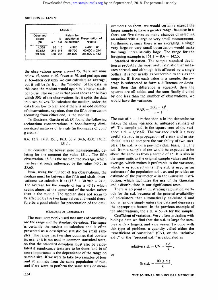
The counters in radiation-counting equipment often have six digits, and the question of how many digits to carry is a bit more complicated. A common rule of thumb is to calculate the square root of the indicated number of counts, which is its s.d., and record only the number of digits to the left of (higher order than) the s.d. If the data are to be used in subsequent calculation, record one extra digit—i.e., carry the equivalent of the high-order digit of the s.d. through computation and round to the appropriate digit at the end of the computation. The standard deviation is usually rounded to the nearest whole number. This rule of thumb, illustrated in Table 1, is based on the concept of retaining as a significant digit the lowest order digit that changes by one-tenth or less. It is consistent with other types of noncounting measurements.

MEASURES OF CENTRAL TENDENCY

Regardless of whether the data that have been gathered are to be used for description (as in the case of many clearance studies) or for inference to a larger population (as in the case of comparison of toxic effects of two compounds), some statistic that characterizes middleness of a set of data is usually required. The most frequent measure of central tendency is the average or sample mean, usually written as x. The Greek letter p, is usually reserved for the population mean, although occasionally the sample mean is written as p. when it is referred to as an estimate of the population mean. If the sample mean is calculated on measurements from a random sample of a larger population, x is then a valid estimate of the population mean. Otherwise, the restrictions regarding what population it is applicable to must be included in any discussion.

There are several instances (particularly if a sample is small) when the sample average would be a misleading measure of central tendency. When there are a few outlying observations ("mavericks") that cannot be discarded because of bad technique or faulty measurement, the median is a more appropriate statistic. Similarly, if a group of data appears to be highly skewed—e.g., if most of




SHELDON G. LEVIN

TABLE 1.

Observed Retain for count CA additional Presentation of

(N) s.d. s.d. calculation results

4,358 66 1.5 4,360 4,400 ± 66 59,682 244 0.4 59,700 60,000 ± 244

204,836 453 0.2 204,800 205,000 ± 453

the observations group around 25, there are none below 15, some at 40, fewer at 50, and perhaps one at 60—then certainly we can calculate an average, but it will be far from the "middle" of the data; in this case the median would again be a better statistic to use. The median is that point above (or below) which 50% of the observations lie; it splits the data into two halves. To calculate the median, order the data from low to high and if there is an odd number of observations, say nine, then the fifth observation (counting from either end) is the median.

To illustrate, Garcia et al. (5) found the following technetium concentrations in bone-forming dimi-neralized matrices often rats (in thousands of cpm/ g tissue):

8.6, 12.8, 14.9, 15.1, 18.3, 30.9, 34.6, 45.0, 140.5, 151.1.

First consider the lowest nine measurements, deleting for the moment the value 151.1. The fifth observation, 18.3, is the median; the average, which has been strongly influenced by the value 140.5, is 35.60.

Now, using the full set of ten observations, the median must be between the fifth and sixth observations; we calculate it as (18.3 -f 30.9)/2 = 24.6. The average for the sample of ten is 47.18 which seems almost at the upper end of the series rather than in the middle. The median does not seem to be affected by the two large values and would therefore be a good choice for presentation of the data.

MEASURES OF VARIABILITY

The most commonly used measures of variability are the range and the standard deviation. The range is certainly the easiest to calculate and is often presented as a descriptive statistic for small samples. The range has two shortcomings that obviate its use: a) it is not used in common statistical tests, so that the standard deviation must also be calculated if significance tests are to be done; and b) of more importance is the dependence of the range on sample size. If we were to take two samples of four and 20 animals from the same population of rats, and if we were to perform the same tests or meas-

554

urements on them, we would certainly expect the larger sample to have a greater range, because in it there are five times as many chances of selecting an animal with a large or very small measurement. Furthermore, since there is no averaging, a single very large or very small observation would make the range unrealistically large. The range for the foregoing example is 151.1 - 8.6 = 142.5.

Standard deviation. The sample standard deviation is probably the most useful statistic that measures spread, and although it is affected by a single outlier, it is not nearly as vulnerable to this as the range is. If, from each value in a sample, the average is subtracted to fornra difference or deviation, then this difference is squared, then the squares are all added and the sum finally divided by one less than the number of observations, we would have the variance:

n - 1

The use of n - 1 rather than n in the denominator makes the same variance an unbiased estimate of a2. The sample s.d. is the square root of the variance: s. d. = WAR. The variance itself is a very useful statistic in propagation of errors and in statistical tests to compare the variability of two samples. The s.d. is on a per-individual basis, i.e., the s.d. from a sample often would be expected to be about the same as from a sample of 15. It is also in the same units as the original sample values and the average, which makes it preferable to the variance, which is in squared.units. The s.d. is used as an estimate of the population s.d., or, and provides an estimate of the parameter o- in the Gaussian distribution, which facilitates the use of the Gaussian and t distributions in our significance tests.

There is no point in illustrating calculation methods for the s.d. because of the general availability of calculators that automatically calculate x and s.d. when one simply enters the data and depresses the appropriate button. In the previous example of ten observations, the s.d. = 53.24 for the sample.

Coefficient of variation. Very often in dealing with biologic data we find that the s.d. is large for samples with a large: x and vice versa. To cope with this type of problem, a quantity called either the "coefficient of variation" (CV), or the "relative s.d.," or the "percent s.d." is calculated as

s.d. relative s.d. = CV = ,

x

or

100 (s.d.) % s.d. = .

x

THE JOURNAL OF NUCLEAR MEDICINE




This is a unitless measure; e.g., in the previous example we calculate

_ . . s.d. 53.24 cpm/mg c v = _ H s = 1.13 or 113% s.d.,

x 47.18 cpm/mg

and we see that the units cancel. In this case, the s.d. is actually larger than the average, an indication of very large variability.

Because the CV is a unitless statistic we can use it to compare our work with that of others to get a feel for how variable our experiment is. A CV of 5-10% is excellent, 10-30% is usual, and 40% or more is excessive. More about this when we come to considerations of sample size.

Standard error of the mean (or "standard error"). We randomly select a sample from a population and make measurements on the sampled items (e.g., animals) to obtain an estimate of the population mean, /x. The more variable the population, the larger the sample that must be taken in order to get the same precision for our estimate of /x. The standard error of the mean is a statistic that describes the variability of the average of samples containing n items. It is written as

Sx = - ^ = , Vn

where we obtain our estimate of o- from the sample s.d. The Vn in the denominator tells us that for very large samples, Sx becomes very small and that it increases as the sample size gets smaller. This makes sense because when one collects several observations to form a sample, the large and small observations are averaged; hence the sample mean tends to be less variable as we include more observations in the sample.

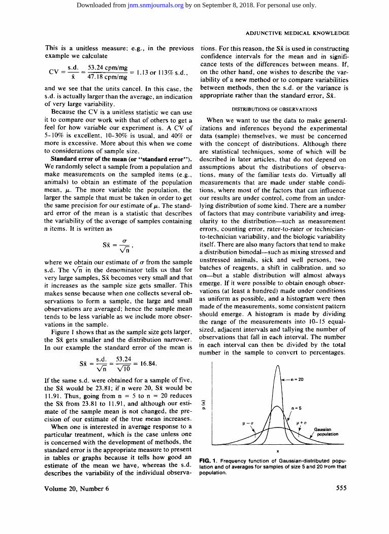
Figure I shows that as the sample size gets larger, the Sx gets smaller and the distribution narrower. In our example the standard error of the mean is

s.d. 53.24 ^ OA Sx=—^= = —F= = 16.84.

Vn >/l0

If the same s.d. were obtained for a sample of five, the Sx would be 23.81; if n were 20, Sx would be 11.91. Thus, going from n = 5 to n = 20 reduces the Sx from 23.81 to 11.91, and although our estimate of the sample mean is not changed, the precision of our estimate of the true mean increases.

When one is interested in average response to a particular treatment, which is the case unless one is concerned with the development of methods, the standard error is the appropriate measure to present in tables or graphs because it tells how good an estimate of the mean we have, whereas the s.d. describes the variability of the individual observa

tions. For this reason, the Sx is used in constructing confidence intervals for the mean and in significance tests of the differences between means. If, on the other hand, one wishes to describe the variability of a new method or to compare variabilities between methods, then the s.d. or the variance is appropriate rather than the standard error, Sx.

DISTRIBUTIONS OF OBSERVATIONS

When we want to use the data to make generalizations and inferences beyond the experimental data (sample) themselves, we must be concerned with the concept of distributions. Although there are statistical techniques, some of which will be described in later articles, that do not depend on assumptions about the distributions of observations, many of the familiar tests do. Virtually all measurements that are made under stable conditions, where most of the factors that can influence our results are under control, come from an underlying distribution of some kind. There are a number of factors that may contribute variability and irregularity to the distribution—such as measurement errors, counting error, rater-to-rater or technician-to-technician variability, and the biologic variability itself. There are also many factors that tend to make a distribution bimodal—such as mixing stressed and unstressed animals, sick and well persons, two batches of reagents, a shift in calibration, and so on—but a stable distribution will almost always emerge. If it were possible to obtain enough observations (at least a hundred) made under conditions as uniform as possible, and a histogram were then made of the measurements, some consistent pattern should emerge. A histogram is made by dividing the range of the measurements into 10-15 equal-sized, adjacent intervals and tallying the number of observations that fall in each interval. The number in each interval can then be divided by the total number in the sample to convert to percentages.

FIG. 1. Frequency function of Gaussian-distributed population and of averages for samples of size 5 and 20 from that population.




SHELDON G. LEVIN

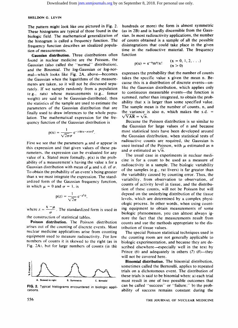
The pattern might look like one pictured in Fig. 2. These histograms are typical of those found in the biologic field. The mathematical generalization of the histogram is called a frequency function. The frequency function describes an idealized population of measurements.

Gaussian distribution. Three distributions often found in nuclear medicine are the Poisson, the Gaussian (also called the "normal'' distribution), and the Binomial. The log-Gaussian or log-normal—which looks like Fig. 2A, above—becomes the Gaussian when the logarithms of the measurements are taken, so it will not be discussed separately. If we sample randomly from a population (e.g., rats) whose measurements (e.g., femur weight) are said to be Gaussian-distributed, then the statistics of the sample are used to estimate the parameters of the Gaussian distribution that are finally used to draw inferences to the whole population. The mathematical expression for the frequency function of the Gaussian distribution is

p(x) = 1TT(T

l /2[( X - M W C T ] 2

First we see that the parameters /* and cr appear in this expression and that given values of these parameters, the expression can be evaluated for any value of x. Stated more formally. p(x) is the probability of a measurement's having the value x for a Gaussian distribution with mean of /n and s.d. of o\ To obtain the probability of an event's being greater than x we must integrate the expression. The standardized form of the Gaussian frequency function, in which jj. ~ 0 and o- = 1, is

p(z)

where z = x -/i

The standardized form is used in

the construction of statistical tables. Poisson distribution. The Poisson distribution

arises out of the counting of discrete events. Most nuclear medicine applications arise from counting equipment used to measure radioactivity. For low numbers of counts it is skewed to the right (as in Fig. 2A). but for large numbers of counts (in the

J ^ A. Skewed to right B. Symmetric

FIG. 2. Typical histograms encountered in biologic applications.

hundreds or more) the form is almost symmetric (as in 2B) and is hardly discernible from the Gaussian. In most radioactivity applications, the number of counts obtained is a sample of all the possible disintegrations that could take place in the given time in the radioactive material. The frequency function

p(x) = e nmx/x! (x = 0, 1,2, . ( n > 0 )

• )

expresses the probability that the number of counts takes the specific value x given the mean n. Because this is a distribution of discrete events—unlike the Gaussian distribution, which applies only to continuous measurable events—the function is summed, rather than integrated, to obtain the probability that x is larger than some specified value. The sample mean is the number of counts, n, and the variance is also n, which makes the s.d. = VVAR = Vn.

Because the Poisson distribution is so similar to the Gaussian for large values of n and because most statistical tests have been developed around the Gaussian distribution, when statistical tests of radioactive counts are required, the Gaussian is used instead of the Poisson, with (x estimated as n and a estimated as \ /n .

The usual case in experiments in nuclear medicine is for a count to be used as a measure of radioactivity in a sample. The biologic variability of the samples (e.g., rat livers) is far greater than the variability caused by counting error. Thus, the variability, from observation to observation, of counts of activity level in tissue, and the distribution of these counts, will not be Poisson but will depend on the underlying distribution of the tissue levels, which are determined by a complex physiologic process. In other words, when using counting equipment to obtain measurements of some biologic phenomenon, you can almost always ignore the fact that the measurements result from counts and use the methods appropriate to the distribution of tissue values.

The special Poisson statistical techniques used in the counting room are not generally applicable to biologic experimentation, and because they are described elsewhere—especially well in the text by Prince (6) and adequately in others (7) (8)—they will not be covered here.

Binomial distribution. The binomial distribution, sometimes called the Bernoulli, applies to repeated trials on a dichotomous event. The distribution of these trials is said to be binomial when: a) each trial must result in one of two possible outcomes that can be called "success" or "failure;" b) the probability of success remains constant during the





course of the experiment; and c) the n trials are independent—i.e., when the outcome of any trial is not dependent on the outcome of any other trial. Examples are: the repeated tossing of a coin, where the outcome is heads or tails; a series of exposures of individuals of a group of homogeneous animals to a fixed level of a toxic substance, where the outcome is live or die; a series of tissue grafts on a set of experimental animals where the outcome can be called success or failure. These examples should follow the binomial distribution. The frequency function is

P(x) = Qpxq"-X (x = 0, 1, . . . , n), (0 < p < /; where

q = I - p and

C£ = n!/x!(n - x)! = . x!(n - x)!

The mean of this distribution is np and the s.d. = %/mpq. The binomial distribution can be used to determine whether the particular set of outcomes from a sample is consistent with a conjectured or previously established value. One very useful application is in the case of determining whether a treatment is effective—i.e., whether a new treatment consistently results in a higher percentage than nontreated. A new treatment is administered to a random sample of 20 persons with the illness, and 15 recover; untreated cases consistently have 50% recovery. Are the results of the new treatment sufficiently better than 50% to be called here p = 0.5, n = 20, x = 15. Using tables of the binomial distribution, we can obtain the probability of exactly 15 successes, or of 15 or more successes, given that the expected proportion of successes is 0.5. From tables [e.g., in (5) (9-11)] we find that the probability of exactly 15 successes is 0.0148. By adding the probabilities for 15 + 16 + . . . + 20 successes—i.e., 0.0148 + 0.0046 + 0.0011 + 0.0001 + 0.0 + 0.0 = 0.0207—we can obtain the probability of at least 15 successes. Thus we can say that the chances of obtaining a result of 15 or more successes because of chance alone (random selection) is about 2 in a hundred, or highly unlikely.

For samples larger than 20, particularly for values of p between 0.30 and 0.70, the distribution is reasonably symmetric and the Gaussian distribution can be used in place of the binomial, with sample mean estimated as x = np and s.d. = Vnpq.

DISTRIBUTIONS OF STATISTICS (SAMPLING DISTRIBUTIONS)

The concept of the distribution of a statistic is a very esoteric one and development in this area has occupied mathematical statisticians for many years. A statistic is not always distributed the same way

as the population of individuals. The simplest and most important case we usually encounter is the distribution of the sample mean, and it will therefore be discussed in more detail than the distribution of other statistics. If measurements on a population from which the sample is randomly drawn are Gaussian-distributed, then regardless of the size of the sample selected, x will be Gaussian-distributed, with mean = fx and s.d. = o-/\/n. Remember that we are talking about the distribution of x and the s.d. of x is called the standard error of the mean, Sx. Therefore, the distributions should look like those in Fig. 1 for n = 1, n = 5 and n = 20.

Central limit theorem. The sample mean has a remarkable property that has most certainly saved many experimenters from embarassment. The central limit theorem tells us that, regardless of the distribution of observations in the population, the distribution of the sample means tends toward (becomes) the Gaussian distribution when the samples are large. For smaller samples (n < 20), the central limit theorem still holds if the population from which we sample is unimodal and more or less symmetric. The theorem tells us that if we suspect the population distribution to be nonGaussian, but we want to use statistical tests requiring that the population be Gaussian distributed (e.g., the t test), then we'd better use a large sample size.

The t distribution. Discussion of the distribution of the sample mean leads to the question of why we use the t distribution if the x is Gaussian-distributed. The Gaussian distribution assumes that the mean /i and the population s.d. cr are known exactly—not just estimated from the sample value. In nuclear medicine applications this is never the case, and fx and cr must be estimated from our data. Therefore, we must have a distribution that takes into consideration the fact that cr is estimated from a sample s.d. and that the estimate of a improves as the sample size increases. William Gosset, who wrote under the name "Student," developed the t distribution to handle this type of problem, and it is probably the most widely used in statistical ap-

plications. The quantity y= is distributed as s.d./vn

Student's t. For large samples (n > 100), the t distribution is

virtually identical with the Gaussian distribution, and in the column called "degrees of freedom" in most t tables, the symbol <*> is the bottom entry. The row associated with that symbol has entries the same as in the Gaussian tables.

Other sampling distributions. In many instances we would like to draw inferences about the variance or the s.d. There are statistics, and they have distributions that have been tabulated and are




SHELDON G. LEVIN

generally available. These distributions have been derived mathematically assuming a Gaussian distribution of the population measurements, and their validity must be taken on faith by nonmathe-maticians. The variance results from squares of deviations, and its frequency function describes what is called the chi-squared (\2) distribution. The chi-squared distribution is also used in statistical tests of dichotomous events, where it is an approximation of the true distribution. The s.d. is not distributed as x2 ' but for large sample sizes it approaches the Gaussian distribution. To compare the variability of two samples, we do not take the difference between two standard deviations, as we take the difference between two xs; instead we take the ratio of two variances, simply because statisticians have developed an exact distribution, Fisher's F, for that ratio, which is valid for all sample sizes.

The major point to be remembered about these distributions is that the measurements must be independent random samples from populations with stable distributions. The populations in nuclear medicine are most often found to have the Poisson, Gaussian, or binomial distribution. Statistics derived from samples of populations where measurements follow these distributions themselves have known and tabulated distributions that we understand and can utilize in making statistical tests of significance or in calculating confidence intervals. The use of the available tabulated values of the sampling distributions will be described in later articles dealing with specific statistical techniques.

APPENDIX

Subsequent articles wilt present, in detail, methods of calculating and interpreting confidence intervals, t tests, and \2 tests, as well as distribution-free equivalents of some of these methods. To fully comprehend these techniques, arm yourself with a calculator, a statistical text with appropriate tables, and some of

your own data; you will then be ready to apply them to your own experimental results.

Although your data should meet criteria of independence, random sampling, etc.. for a do-it-yourself example, these restrictions can be relaxed. Get two independent sets of data, with five to ten observations in each, for confidence intervals and t tests, and if there are occasional "mavericks" present, so much the better. A set of five to ten observations of the "before and after treatment" type will be perfect for the paired t-test.

Most of the references included here are texts of applied statistics that are generally available: some should be found in medical libraries. References 10 and 13 have biologic applications; references 3 .11, and 12 are good general texts that have excellent tables, including random number sequences, t, \2, F, and binomial distributions. References 2 and 9 are handbooks.

REFERENCES

/. EDGINGTON ES: Statistical Interference: The Distribution-free Approach, New York, McGraw-Hill, 1969

2. DIEM K, ed: Documenta Geigy Scientific Tables. Basel, Switzerland, JR Geigy, 1970

3. DIXON WJ, MASSEY FJ: Introduction to Statistical Analysis, New York, McGraw-Hill, 1957

4. WALKER HM, LEV J: Statistical Inference, New York, Henry Holt, 1953

5. GARCIA DA, Tow DE, KAPUR KK, et al.: Relative accretion of 99mTc-polyphosphate by forming and resorbing bone systems in rats: Its significance in the pathologic basis of bone scanning: J Nucl Med 17: 93-97, 1976

6. PRINCE JR, SCHMIDT LD: Statistics and Mathematics in the Nuclear Medicine Laboratory, Chicago, American Society of Clinical Pathology, 1976

7. EVANS RD: The Atomic Nucleus: New York, McGraw-Hill, 1955. pp 746-818

8. MARTIN PM: Nuclear Medicine Statistics: Nuclear Medicine Physics, Instrumentation and Agents, Rollo FD, ed., St. Louis, CV Mosby, 1977, pp 479-512

9. ODEN RE, OWEN DB, BIRNBAUM ZW, et al: Pocketbook of

Statistical Tables, New York. Marcel Dekker, 1977 10. BROWN WB, HOLLANDER M: Statistics: A Biomedical In

troduction. New York, John Wiley and Sons, 1977 / / . WONNACOTT TH, WONNACOTT RJ: Introductory Statistics,

New York, John Wiley, 1977 12. GUENTHER WC: Concepts of Statistical Inference. New

York, McGraw-Hill, 1965 13. CAMPBELL RC: Statistics for Biologists, London, Cambridge

University Press, 1967




Accepted Articles to Appear in Upcoming Issues

Comparison of Wall Motion and Regional Ejection Fraction at Rest and During Isometric Exercise: Concise Communication. Accepted 10/26/78.

Monty M. Bodenheimer, Vidya S. Banka, Colleen M. Fooshee, George A. Hermann, and Richard H. Helfant

Improvement of Pulse-mode Photographic Images in MDS Computer Systems. Accepted 11/8/78.

Michael F. Gard and Charles R. Morris Single-slice Contrasted with Multiple-slice Positron Tomographs (Letter to the Editor). Accepted 1/5/79.

Nizar A. Mullani and John O. Eichling Reply. Accepted 1/5/79.

Michael E. Phelps, Edward J. Hoffman, Sung-cheng Huang The Value of Radionuclide Angiography in the Evaluation of Suspected False Aneurysms (Letter to the Editor). Accepted 1/ 5/79.

Joachim F. Sailer and George B. McDonald Comparison of the Liver's Respiratory Motion in the Supine and Upright Positions: Concise Communication. Accepted 1/9/79.

G. Harauz and M.J . Bronskill Reliability of Gated Heart Scintigrams for Detection of Left-Ventricular Aneurysm: Concise Communication. Accepted 1/11/ 79.

Martin L. Friedman and Robert E. Cantor Radioiodinated DNA as a Potential-Tumor-Imaging Agent. Accepted 1/12/79.

Dionyssis S. Ithakissios and Bern Hapke Transmission Computerized Tomography and Serial Scintigraphy in Intracranial Tumors: What is the Desirable State of the Art? Accepted 1/12/79.

Udalrich Buell and Ekkehard Kazner Radioimmunoassay of Hair for Determining Opiate-Abuse Histories. Accepted 1/15/79.

Annette M. Baumgartner, Peter F. Jones, Werner A. Baum-gartner, and Charles T. Black

Mechanisms of Skeletal Tracer Uptake. Accepted 1/16/79. N. David Charkes

Scintiphotos in Rabbits Made with Tc-99m Preparations Reduced by Electrolysis and by SnCl2: Concise Communication. Accepted 1/17/79.

Joseph Steigman, Edward V. Chin, and Nathan A. Solomon Labeling Efficiency and Stomach Concentration in Methylene Diphosphonate Bone Imaging. Accepted 1/23/79.

Vijay Dhawan and Samuel D. J. Yeh Biodistribution and Pharmacokinetics of S-35-labeIed 5-thio-D-glucose in Hamsters Bearing Pancreatic Tumors. Accepted 1/23/ 79.

Arnold M. Markoe, Victor R. Risch, Ned D. Heindel, Jacqueline Emrich, Wendy Lippincott, Takashi Honda, and Luther W. Brady

Reticuloendothelial Distribution of a Colloid-like Material in 6/3-[13,]-Iodomethyl-19-Norcholesterol (NP-59) (Letter to the Editor). Accepted 1/24/79.

Hank Chilton, Jon C. Lewis, Steven F. Motsinger, and Robert J. Cowan

Altered Biodistribution of 6/3-[131]Iodomethyl-19-Norcholesterol

(NP-59): Radiopharmaceutical Contamination or Patient Idio-syncracy? (Letter to the Editor). Accepted 1/24/79.

Dennis P. Swanson, Nancy E. Wirth, and Milton D. Gross Reply. Accepted 1/24/79.

Hank Chilton, Jon C. Lewis. Stephen F. Motsinger, and Robert J. Cowan

Optimization of Analog-Circuit Motion Correction for Liver Scintigraphy (Letter to the Editor). Accepted 1/24/79.

R. F. Mould Reply. Accepted 1/24/79.

M. J. Bronskill Scintigraphic, Electrocardiographic, and Enzymatic Diagnosis of Perioperative Myocardial Infarction in Patients Undergoing Myocardial Revascularization. Accepted 1/25/79.

John A. Burdine, E. Gordon DePuey, Fulvio Orzan. Virendra S. Mathur, and Robert J. Hall

Accidental Ingestion of Tc-99m in Breast Milk by a 10-Week-Old Child (Letter to the Editor). Accepted 1/25/79.

Aslam R. Siddiqui Reply. Accepted 1/25/79.

Warren F. Rumble [nC]Methionine Pancreatic Scanning with Positron Emission Computed Tomography. Accepted 1/26/79.

Andre Syrota, Dominique Comar, Marc Cerf, David Plummer, Mariannick Maziere, and Claude Kellershohn

1-125 Fibrinogen Test Complicated by Allergic Dermatitis Caused by Skin Marker (Letter to the Editor). Accepted 1/31/ 79.

Donald W. Brown Quantitative Scanning of Osteogenic Sarcoma with Nitrogen-13-Labeled L-Glutamate. Accepted 2/1/79.

A. S. Gelbard, R. S. Benua, J. S. Laughlin, G. Rosen, R. E. Reiman, and J. M. McDonald

Computer-Assisted Liver Mass Estimation from Gamma Camera Images (Letter to the Editor). Accepted 2/9/79.

Edward A. Eikman Regional Ventilatory Clearance by Xenon Scintigraphy: A Critical Evaluation of Two Estimation Procedures. Accepted 2/14/ 79.

Barry Bunow, Bruce R. Line, Martha R. Horton, and George H. Weiss

Single-Photon Transaxial Emission Computed Tomography of the Heart in Normal Subjects and in Patients with Infarction. Accepted 2/15/79.

B. Leonard Holman, Thomas C. Hill, Joshua Wynne, Richard D. Lovett, Robert E. Zimmerman, and Edward M. Smith

"Circumferential Profiles:" A New Method for Computer Analysis of Thallium-201 Myocardial Perfusion Images. Accepted 2/ 20/79.

Robert D. Burow, Malcolm Pond, A. William Schafer, and Lewis Becker

Indium-lll-Labeled Human Polymorphonuclear Leukocytes: Viability, Random Migration, Chemotaxis, Bactericidal Capacity, and Ultrastructure. Accepted 2/21/79.

Behnam Zakireh, Mathew L. Thakur, Harry L. Malech, Myron S. Cohen, Alexander Gottschalk, and Richard K. Root




1979;20:550-559.J Nucl Med. Sheldon G. Levin Understanding and Using Statistics in Nuclear Medicine

http://jnm.snmjournals.org/content/20/6/550.citationThis article and updated information are available at:

http://jnm.snmjournals.org/site/subscriptions/online.xhtml

Information about subscriptions to JNM can be found at:

http://jnm.snmjournals.org/site/misc/permission.xhtmlInformation about reproducing figures, tables, or other portions of this article can be found online at:

(Print ISSN: 0161-5505, Online ISSN: 2159-662X)1850 Samuel Morse Drive, Reston, VA 20190.SNMMI | Society of Nuclear Medicine and Molecular Imaging

is published monthly.The Journal of Nuclear Medicine

© Copyright 1979 SNMMI; all rights reserved.


http://jnm.snmjournals.org/content/20/6/550.citation

http://jnm.snmjournals.org/site/misc/permission.xhtml

http://jnm.snmjournals.org/site/subscriptions/online.xhtml


Documents

Understanding and Using Statistics in Nuclear Medicinejnm.snmjournals.org/content/20/6/550.full.pdf · Understanding and Using Statistics in Nuclear Medicine Sheldon G. Levin Armed