Understanding rainfall projections in relation to

Australian Meteorological and Oceanographic Journal 63 (2013) 355–364

355

Understanding rainfall projections in relation to extratropical cyclones in eastern Australia

Andrew J. Dowdy, Graham A. Mills, Bertrand Timbal, Morwenna Griffiths and Yang Wang

Centre for Australian Weather and Climate Research, Melbourne, Australia

(Manuscript received August 2012; revised March 2013)

Heavy rainfall events along Australia’s eastern seaboard are often associated with the occurrence of extratropical cyclones known as East Coast Lows. Such rain-fall events contribute significantly to runoff and water availability, with conse-quences that can be beneficial (increased water storage), but also can cause major adverse effects due to both flash floods and widespread inundation. Any trends in the frequency of such rainfall events into the future are thus of great importance in planning. Gridded analyses of rainfall observations are used to develop three different heavy rainfall climatologies along Australia’s eastern seaboard. These heavy rainfall climatologies have contrasting spatial characteristics to each other and are complemented by river-flow observations to identify large inflow events. A diagnostic of the likelihood of East Coast Low occurrence, based on reanalysis data and of a scale previously shown to be sufficiently large to be resolved by global climate models, is adapted to examine its ability to represent the occur-rence of these heavy rainfall and river inflow events. The diagnostic is found to provide a useful means of identifying the likelihood of occurrence of heavy rainfall events, indicating an increasing proportion of heavy rainfall events for increasing rainfall amounts. Seasonal and regional variability of both the diagnostic and the various heavy rainfall classes are examined. The diagnostic is then applied to a global climate model (HadCM3.0) simulation of the current and future climate to examine the influence of increasing atmospheric greenhouse gas concentrations on heavy rainfall and inflow events associated with extratropical cyclones in this region. The results indicate that the frequency of these particular classes of heavy rain events could be expected to decrease by between about eight and 25 per cent, depending on season and latitude, by the end of the 21st century for a high emis-sions scenario. Results are compared to the global climate model direct simula-tions of the expected changes in rainfall from the 20th to 21st century.

Introduction

The climate of the eastern seaboard of Australia is distinct from the rest of eastern Australia, with rainfall on the eastern seaboard not following the same relationships with large-scale environmental influences such as the El Niño–Southern Oscillation (ENSO) as occurs throughout other parts of eastern Australia (Timbal 2010, Timbal and Hendon 2011). Extreme weather events in this region are often associated with the occurrence of intense extratropical cyclones known as East Coast Lows (ECLs), including heavy rainfall, strong wind and severe wave events (McInnes et al. 1992, Short and Treneman

1992, Hopkins and Holland 1997, McInnes et al. 2002, Speer 2008, Mills et al. 2010). Additionally, major inflows to Sydney’s water storages have been shown to be associated with rainfall generated during ECL events (Pepler and Rakich 2010).

Modeling of heavy rainfall is a complex problem, with very large uncertainty often being associated with the upper end of the rainfall distribution. For example, Pitman and Perkins (2008) found that the variation between the different Global Climate Models (GCMs) they examined from the CMIP3 simulations was of order ten times greater in the 99.7th percentile than in the mean rainfall. Some studies have also suggested changes in the frequency and in the magnitude of heavy rainfall events in the Sydney region may be opposite in sign to each other (Jakob et al. 2011).

The Fourth Assessment Report from the Intergovernmental Panel on Climate Change (Solomon et

Corresponding author address: Andrew Dowdy, Bureau of Meteorology, 700 Collins Street, Docklands, Victoria 3008, Australia. E-mail: [email protected]

356 Australian Meteorological and Oceanographic Journal 63:3 September 2013

(i) Localised and widespread rain eventsFor each region, a given day was defined as having a ‘localised rain event’ if the maximum rainfall at a single grid point within the region was above the 90th percentile of this quantity calculated for the study period over this region. Similarly, a ‘widespread rain event’ is considered to have occurred for a given day and region if the sum of the rainfall at all grid points within a particular region is above the 90th percentile of this quantity for that region, with the rainfall volume sum calculated by assuming that each millimetre of rainfall at a grid point occurred consistently throughout the gridded region (with 0.05 degree resolution in both latitude and longitude). The 90th percentile threshold values used to define localised and widespread rain events are shown for each region and season (Table 1), with summer and winter referring throughout this study to the periods from November to April and from May to October, respectively.

(ii) Cluster rain eventsThe above event types may not necessarily identify the types of relatively small, but intense, rainbands that can sometimes be associated with ECLs, an example of which is shown in Fig. 3 of Mills et al. (2010). Accordingly, a third type of heavy rainfall event, referred to as a ‘cluster rain event’, was also derived from AWAP rainfall analyses based on a clustering algorithm. These rainfall clusters identify significant rainfall events that are larger in scale than thunderstorm scale, while significantly smaller in scale than the regions shown in Fig. 1 used to determine widespread rain events.

The first step in the clustering algorithm is to identify AWAP rainfall analysis grid-points where the daily rainfall is above 1 mm. For grid-points that meet this criterion, the sum of the rainfall at all adjoining grid-points which also have more than 1 mm rainfall is calculated. This leads to a number of distinct rainfall entities being identified across the analysis grid. A rainfall entity is discarded if its summed

al. 2007) puts a critical emphasis on extreme events, with many of the consequences of anthropogenic climate change expected to be experienced through changes in extreme event occurrence. However, assessing the climatology of extreme events such as extratropical cyclones and associated severe weather impacts is currently a field that is not well-represented in the literature.

GCMs can provide a good representation of the large-scale general circulation of the atmosphere, but currently do not have sufficient resolution to adequately represent phenomena such as ECLs and the scales or intensity of their associated (often extreme) rainfall events. Due to the abilities and limitations of current GCMs, a large-scale diagnostic of the likelihood of ECL occurrence was recently developed based on 500 hPa geostrophic vorticity (Dowdy et al. 2013a) and shown to be large enough in spatial and temporal scale to be applicable to GCMs (Dowdy et al. 2013b). The connection that was identified in these studies between ECL occurrence and the presence of strong upper-tropospheric cyclonic vorticity poses the question as to whether or not changes in the occurrence of heavy rainfall and river inflows can be associated with changes in the occurrence of strong upper-tropospheric cyclonic vorticity events.

This study uses analyses of rainfall and streamflow observations to categorise a number of different heavy rainfall event types for the eastern seaboard region. The ability of a diagnostic, based on upper-tropospheric cyclonic vorticity, to represent heavy rainfall events is examined by applying the diagnostic to reanalyses for the period 1979 to 2010, and comparing this with the occurrence of heavy rainfall events. Seasonal and regional variability is examined. The diagnostic is then applied to GCM simulations of the current and future climate to examine the influence of increasing atmospheric greenhouse gas concentrations on heavy rainfall events in the eastern seaboard region.

Data and methodology

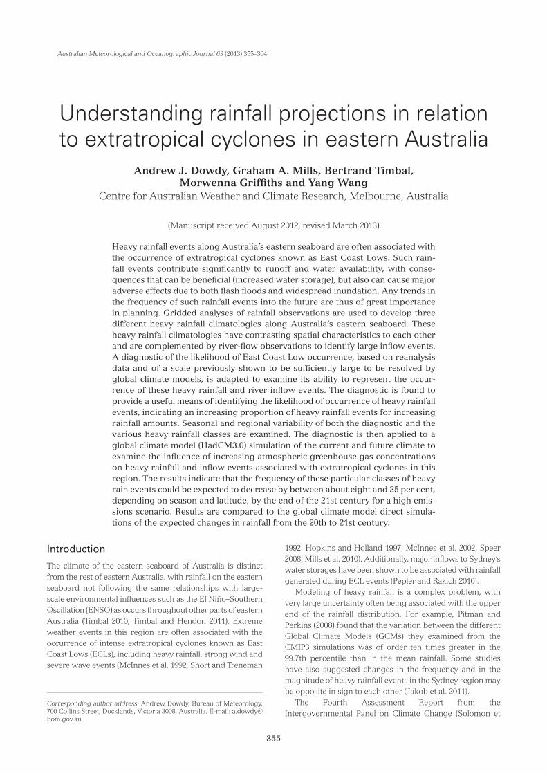
Rainfall climatologiesHeavy rainfall events are examined for two different regions within the eastern seaboard of Australia (Fig. 1), each spanning 5° latitude: the ‘northern region’ (within the latitude range 28°S to 33°S) and the ‘southern region’ (within the latitude range 33°S to 38°S). The western boundary of these regions is the ridge line of the Great Dividing Range (truncated to 147.5°E as the focus of this study is on the eastern seaboard region), with the eastern boundary being the coastline.

Rainfall data were obtained from the Australian Water Availability Project (AWAP) gridded analyses of rainfall observations covering the period 1979 to 2010 (Jones et al. 2009). This dataset consists of daily rainfall gridded at 0.05° resolution throughout Australia (approximately 5 km resolution in both latitude and longitude), with the rainfall valid for the 24-hour period from 9.00 am to 9.00 am Local Time (LT).

Fig. 1. Map of the eastern seaboard showing the two sub-regions used in this study: the northern region (yel-low) and the southern region (green). State borders, capital cities, latitude and longitude are shown.

Dowdy et al.: Understanding rainfall projections in relation to extratropical cyclones in eastern Australia 357

the above methodology results in data being available for at least one site on all days within each of the two regions.

In order to examine large inflow events in each of the two regions, the daily streamflow data were first converted to daily time series of inflow, with the inflow calculated for each day as the change in streamflow from the previous day to that day. The resultant time series are then converted to percentile values, calculated individually for each streamflow site, so as to equally weight data from sites with different mean streamflows. Daily time series are then produced of the maximum streamflow in each region, based on the highest daily percentile value from all sites within the region. Days on which the inflow is above its 90th percentile value for a particular region are defined here as ‘large inflow events’. This methodology identifies the initial stream-rise resulting from a rainfall event, as we are matching this metric with rainfall events, and is not intended to identify sustained periods of high streamflow.

rainfall is less than 1000 mm, so as to exclude the very small entities. If any of the remaining rainfall entities are located within 120 km of each other they are considered to be part of a single combined entity.

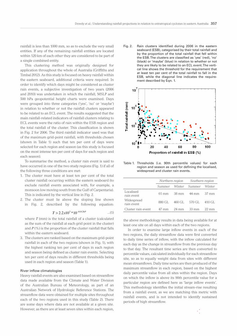
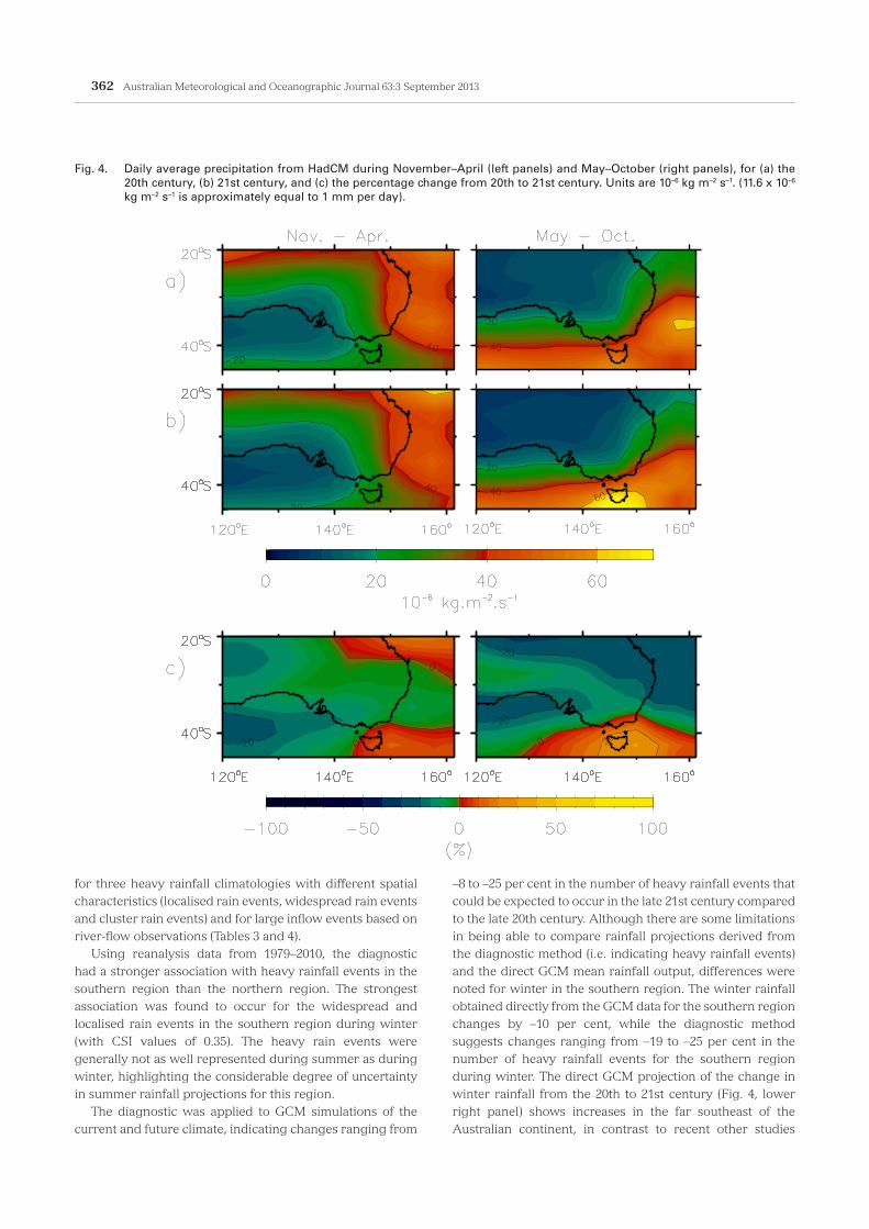
This clustering method was originally designed for application throughout the whole of Australia (Griffiths and Timbal 2012). As this study is focused on heavy rainfall within the eastern seaboard, additional criteria were required. In order to identify which days might be considered as cluster rain events, a subjective investigation of two years (2006 and 2010) was undertaken in which the rainfall, MSLP and 500 hPa geopotential height charts were examined. Days were grouped into three categories (‘yes’, ‘no’ or ‘maybe’) in relation to whether or not the rainfall clusters appeared to be related to an ECL event. The results suggested that the main rainfall-related indicators of rainfall clusters relating to ECL events were the ratio of rain within the ESB region and the total rainfall of the cluster. This classification is shown in Fig. 2 for 2006. The third rainfall indicator used was that of the maximum grid-point rainfall, with thresholds chosen (shown in Table 1) such that ten per cent of days were selected for each region and season (as this study is focused on the most intense ten per cent of days for each region and each season).

To summarise the method, a cluster rain event is said to have occurred in one of the two study regions (Fig. 1) if all of the following three conditions are met:1. The cluster must have at least ten per cent of the total

cluster rainfall occurring within the eastern seaboard (to exclude rainfall events associated with, for example, a monsoon low moving south from the Gulf of Carpentaria). This is indicated by the vertical line in Fig. 2.

2. The cluster must lie above the sloping line shown in Fig. 2, described by the following equation:

...(1)T > 2.2x105 *10−0.0128P

where T (mm) is the total rainfall of a cluster (calculated as the sum of the rainfall at each grid point in the cluster) and P (%) is the proportion of the cluster rainfall that falls within the eastern seaboard.

3. The clusters are ranked based on the maximum grid-point rainfall in each of the two regions (shown in Fig. 1), with the highest ranking ten per cent of days in each region and season being defined as cluster rain events. Selecting ten per cent of days results in different thresholds being used in each region and season (Table 1).

River inflow climatologiesHeavy rainfall events are also examined based on streamflow data made available from the Climate and Water Division of the Australian Bureau of Meteorology, as part of an Australian Network of Hydrologic Reference Stations. The streamflow data were obtained for multiple sites throughout each of the two regions used in this study (Table 2). There are some days where data are not available at a given site. However, as there are at least seven sites within each region,

Fig. 2. Rain clusters identified during 2006 in the eastern seaboard (ESB), categorised by their total rainfall and by the proportion of the total rainfall that fell within the ESB. The clusters are classified as ‘yes’ (red), ‘no’ (black) or ‘maybe’ (blue) in relation to whether or not they are likely to be related to an ECL event. The verti-cal line shows the threshold for the requirement that at least ten per cent of the total rainfall to fall in the ESB, while the diagonal line indicates the require-ment described by Eqn. 1.

Table 1. Thresholds (i.e. 90th percentile values) for each region and season as used for defining the localised, widespread and cluster rain events.

Northern region Southern region

Summer Winter Summer Winter

Localised rain event

61 mm 38 mm 44 mm 37 mm

Widespread rain event

880 GL 460 GL 570 GL 410 GL

Cluster rain event 47 mm 24 mm 33 mm 22 mm


of 15° in longitude and 10.5° in latitude. As described in Dowdy et al. (2013a), the centre of this box is determined dynamically and can vary slightly for different event definitions and seasons, and examples of this are presented later in this paper (Tables 3 and 4). The minimum value of vorticity is selected as this represents the maximum cyclonic vorticity, given that cyclonic vorticity is negative in sign for the southern hemisphere.

The diagnostic is calculated from ERA-Interim reanalyses for the period 1979 to 2010 (ERAI, Uppala et al. 2008), with six-hourly temporal and 1.5 degree spatial resolution. A one-day running-mean is applied to the six-hourly diagnostic time series to reduce small-scale temporal variability, as the purpose of this study is to use a diagnostic method large enough in scale (spatial and temporal) to be suitable for potential application to GCMs. Days on which the time series exceeds a threshold value, selected as being above the 90th percentile of cyclonic geostrophic vorticity, are defined as being indicative of the likely occurrence of ECL formation. This percentile level (i.e. selecting one day in ten on average) was chosen as detailed in Dowdy et al. (2011), based on an examination of time series of the diagnostic in relation to days on which ECLs were listed to have occurred in the Speer et al. (2009) dataset of observed ECL events, with approximately one in ten days on average being listed in the dataset as corresponding to an ECL event (noting that many ECLs last for multiple days).

To match the diagnostic events to the heavy rain events, consecutive days where the diagnostic exceeds its threshold are considered as a single diagnostic event. This is also the case for the heavy rain events, with consecutive event

Diagnostic methodologyThe diagnostic developed by Dowdy et al. (2011) is based on upper-tropospheric geostrophic vorticity, ξ, calculated as the Laplacian of geopotential divided by the Coriolis parameter:

ξ = 1f∇2Φ ...(2)

where f is the Coriolis Parameter and ∇2Φ the Laplacian of geopotential.

This particular diagnostic quantity was selected based on a systematic examination of a range of potential diagnostic quantities in relation to an observed data-base of ECL occurrence (Speer et al. 2009). In addition to geostrophic vorticity, other potential diagnostics examined included isentropic potential vorticity (at isobaric and isentropic levels) and the forcing term of the pseudo-potential vorticity form of the quasi-geostrophic height tendency equation (following Bluestein 1992, Eqn 5.8.15), with diagnostic skill assessed for each diagnostic quantity at a number of different levels in the upper troposphere (Dowdy et al. 2013a). A variety of other potential diagnostic measures of extratropical cyclogenesis were also examined, including baroclinicity measures such as the Eady Growth Rate (Eady 1949), although applying the diagnostic method (as used for geostrophic vorticity) to the Eady Growth Rate did not show as strong a relationship with the observed ECL data-base as occurs for the diagnostic based on geostrophic vorticity (Dowdy et al. 2013b).

The diagnostic is produced by first calculating a time series of the minimum (i.e. strongest cyclonic) value of the 500 hPa geostrophic vorticity within a geographic region

Table 2. Site names for the streamflow data, including location (latitude, longitude) and region.

Streamflow site name Lat. (˚S) Lon. (˚E) Region

Henry River at Newton Boyd 29.8 152.2 Northern

Wollomombi River at Coninside 30.5 152.0 Northern

Apsley River at Apsley Falls 31.1 151.8 Northern

Nowendoc River at Nowendoc 31.5 151.7 Northern

Barnard River at Barry 31.6 151.3 Northern

Goulburn River at Coggan 32.3 150.1 Northern

Williams River at Tillegra 32.3 151.7 Northern

Jigadee Creek at Avondale 33.1 151.5 Southern

Kowmung River at Cedar Ford 33.9 150.2 Southern

Nepean River at Maguires Crossing 34.5 150.5 Southern

Currambene Creek at Falls Creek 35.0 150.6 Southern

Corang River at Hockeys 35.1 150.0 Southern

Shoalhaven River at Warri 35.3 149.7 Southern

Clyde River at Brooman 35.5 150.2 Southern

Tuross River at Tuross Vale 36.3 149.5 Southern

Rutherford Creek at Brown Mountain 36.6 149.4 Southern

Genoa River at The Gorge 37.4 149.5 Southern

Errinundra River at Errinundra 37.4 148.9 Southern


UTC) for time slices from 1960 to 1988 and 2070 to 2098. This grid resolution allows a diagnostic box of 10° latitude by 15° longitude, a close match to the size of the diagnostic box used for the ERAI reanalyses, albeit with less grid-points. The 21st century simulation used in this study is based on a high emission scenario, A2. The global average temperature rise for the A2 scenario is expected to be of the order of 2.0 °C to 5.4 °C by the end of the 21st century (Solomon et al. 2007), with the temperature range reflecting the range of sensitivities of the various CMIP3 climate models to the external forcings. The sensitivity of the HadCM model is near the middle of the range of sensitivities of the CMIP3 models (e.g. CSIRO and Bureau of Meteorology 2007, Table 4.1).

Results

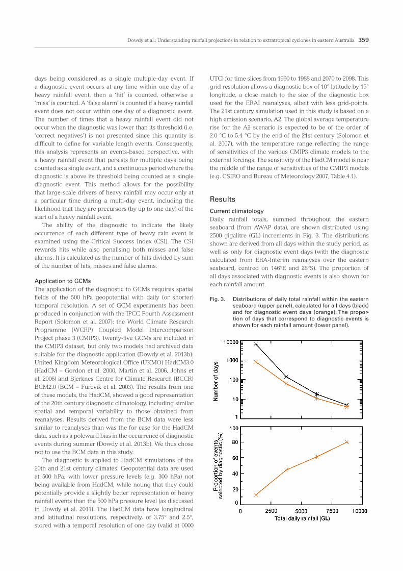
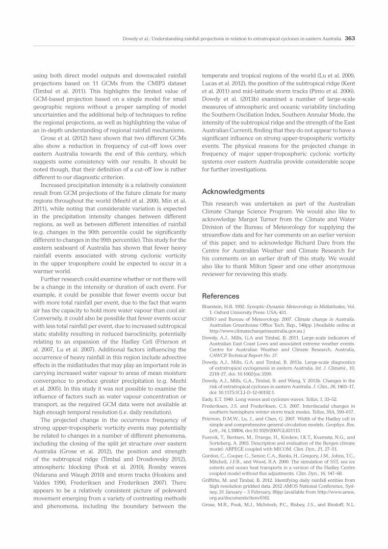
Current climatologyDaily rainfall totals, summed throughout the eastern seaboard (from AWAP data), are shown distributed using 2500 gigalitre (GL) increments in Fig. 3. The distributions shown are derived from all days within the study period, as well as only for diagnostic event days (with the diagnostic calculated from ERA-Interim reanalyses over the eastern seaboard, centred on 146°E and 28°S). The proportion of all days associated with diagnostic events is also shown for each rainfall amount.

days being considered as a single multiple-day event. If a diagnostic event occurs at any time within one day of a heavy rainfall event, then a ‘hit’ is counted, otherwise a ‘miss’ is counted. A ‘false alarm’ is counted if a heavy rainfall event does not occur within one day of a diagnostic event. The number of times that a heavy rainfall event did not occur when the diagnostic was lower than its threshold (i.e. ‘correct negatives’) is not presented since this quantity is difficult to define for variable length events. Consequently, this analysis represents an events-based perspective, with a heavy rainfall event that persists for multiple days being counted as a single event, and a continuous period where the diagnostic is above its threshold being counted as a single diagnostic event. This method allows for the possibility that large-scale drivers of heavy rainfall may occur only at a particular time during a multi-day event, including the likelihood that they are precursors (by up to one day) of the start of a heavy rainfall event.

The ability of the diagnostic to indicate the likely occurrence of each different type of heavy rain event is examined using the Critical Success Index (CSI). The CSI rewards hits while also penalising both misses and false alarms. It is calculated as the number of hits divided by sum of the number of hits, misses and false alarms.

Application to GCMsThe application of the diagnostic to GCMs requires spatial fields of the 500 hPa geopotential with daily (or shorter) temporal resolution. A set of GCM experiments has been produced in conjunction with the IPCC Fourth Assessment Report (Solomon et al. 2007): the World Climate Research Programme (WCRP) Coupled Model Intercomparison Project phase 3 (CMIP3). Twenty-five GCMs are included in the CMIP3 dataset, but only two models had archived data suitable for the diagnostic application (Dowdy et al. 2013b): United Kingdom Meteorological Office (UKMO) HadCM3.0 (HadCM – Gordon et al. 2000, Martin et al. 2006, Johns et al. 2006) and Bjerknes Centre for Climate Research (BCCR) BCM2.0 (BCM – Furevik et al. 2003). The results from one of these models, the HadCM, showed a good representation of the 20th century diagnostic climatology, including similar spatial and temporal variability to those obtained from reanalyses. Results derived from the BCM data were less similar to reanalyses than was the for case for the HadCM data, such as a poleward bias in the occurrence of diagnostic events during summer (Dowdy et al. 2013b). We thus chose not to use the BCM data in this study.

The diagnostic is applied to HadCM simulations of the 20th and 21st century climates. Geopotential data are used at 500 hPa, with lower pressure levels (e.g. 300 hPa) not being available from HadCM, while noting that they could potentially provide a slightly better representation of heavy rainfall events than the 500 hPa pressure level (as discussed in Dowdy et al. 2011). The HadCM data have longitudinal and latitudinal resolutions, respectively, of 3.75° and 2.5°, stored with a temporal resolution of one day (valid at 0000

Fig. 3. Distributions of daily total rainfall within the eastern seaboard (upper panel), calculated for all days (black) and for diagnostic event days (orange). The propor-tion of days that correspond to diagnostic events is shown for each rainfall amount (lower panel).


The diagnostic generally produces better results during winter (0.29 ≤ CSI ≤ 0.35) than summer (0.21 ≤ CSI ≤ 0.33). Better results are also generally obtained in the southern region (0.27 ≤ CSI ≤ 0.35) than in the northern region (0.21 ≤ CSI ≤ 0.33). The best result for any region, season and event type occurs for the widespread and localised rain events during winter in the southern region, corresponding to CSI = 0.35 for both event types.

The location of the best diagnostic region tends to occur northwest of the eastern seaboard. There is some indication that the best diagnostic location tends to be further north for the northern region than for the southern region.

Future climate projectionsThe change in the occurrence frequency of diagnostic events from the 20th to 21st century (Table 5) was calculated from HadCM data at the locations closest to those listed in Tables 3 and 4. The 90th percentile of the diagnostic calculated for the 20th century was used as the threshold for defining diagnostic events for both the 20th and 21st centuries. This method avoids the issue of whether the climate model correctly identifies cut-off low frequency in the 20th century (as addressed for different climate models by Grose et al. 2012).

For increasing rainfall amounts, the diagnostic events correspond to an increasing proportion of heavy rainfall events, with values of up to about 60–80 per cent for the highest rainfall amounts. This result shows that the presence of strong upper-tropospheric cyclonic vorticity provides a useful indication of the likelihood of occurrence of heavy rain events.

To allow for the possibility that the best diagnostic location is variable between different regions, seasons and heavy rainfall types, the diagnostic region (spanning 15 degrees of longitude and 10.5 degrees of latitude) can be centred on different locations when calculating the diagnostic event days (Dowdy et al. 2011). This is done individually for each grid point of the ERA-Interim dataset in the vicinity of the eastern seaboard (covering the region from 135°E to 168°E in longitude and 43°S to 19°S in latitude). For each of these grid-points, the ability of the diagnostic method to correctly identify the occurrence or non-occurrence of a heavy rainfall event is calculated using the CSI. The latitude and longitude of the centre of the geographic box used to calculate the diagnostic that produced the maximum CSI value is shown in Tables 3 and 4. Results are shown individually for each type of heavy rainfall event, in each region, during summer and winter.

Table 3. Diagnostic performance during the summer period for each of the four heavy rain event types, in each of the two regions. The maximum CSI value is shown in each case, together with the corresponding number of hits, misses and false alarms, as well as the location of the centre of the diagnostic region that produced the maximum CSI value. Results that have a higher degree of confidence associated with them (based on CSI ≥ 0.30) are highlighted in bold font.

Region Max. CSI Hit Miss False alarm Latitude of max. CSI

Longitude of max. CSI


Northern 0.21 91 212 128 22˚S 147˚E

Southern 0.30 127 195 97 29˚S 144˚E


Northern 0.21 91 233 104 25˚S 141˚E

Southern 0.33 145 204 90 29˚S 143˚E

Cluster rain eventNorthern 0.21 93 223 127 29˚S 146˚E

Southern 0.31 128 201 89 29˚S 146˚E

Large inflow eventNorthern 0.21 99 222 149 31˚S 141˚E

Southern 0.27 113 194 110 29˚S 146˚E

Table 4. As for Table 3, but for winter.

Region Max. CSI Hit Miss False alarm Latitude of max. CSI

Longitude of max. CSI


Northern 0.29 164 234 165 25˚S 143˚E

Southern 0.35 186 200 141 28˚S 141˚E


Northern 0.32 164 181 165 26˚S 138˚E

Southern 0.35 169 164 153 26˚S 141˚E

Cluster rain eventNorthern 0.33 162 186 150 25˚S 144˚E

Southern 0.33 162 180 154 28˚S 141˚E

Large inflow eventNorthern 0.31 147 149 171 26˚S 146˚E

Southern 0.33 149 134 170 26˚S 143˚E


change in diagnostic events (from Table 5) multiplied by the corresponding hit rate (from Tables 3 and 4).

For the results that have the higher confidence associated with them (shown in bold font in Table 6), the projected changes in heavy rainfall occurrence during winter range from –19 to –25 per cent for the southern region and from –19 to –24 per cent for the northern region, while during summer the changes are from –8 to –11 per cent for the southern region.

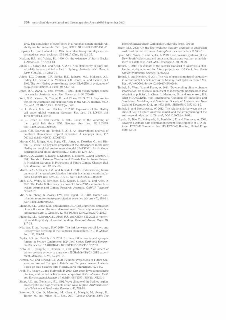
Even though it is not expected that current GCMs produce highly accurate representations of features such as regional rainfall, it is still of general interest to examine the change in mean rainfall obtained directly from HadCM. This is shown in Fig. 4 as well as in Table 6, with the direct GCM projections based on the average value for all grid-points in the northern and southern regions. The rainfall changes derived directly from the GCM are –3 and –8 per cent during summer, and –10 and –17 per cent during winter (Table 6). While noting that the results derived from the diagnostic do not include the influence of potential changes in other rain producing factors (e.g. thunderstorms), as well as recognising the differences between heavy rainfall (indicated by the diagnostic) and mean rainfall (obtained directly from the GCM), the change of –10 per cent for the southern region during winter is somewhat less than the corresponding changes from –19 to –25 per cent in heavy rainfall events indicated by the diagnostic (noting from Table 4 that this is the region and time of year that the diagnostic produces the best results). The relatively small reduction in rainfall for the southern region during winter indicated by the direct model output is in part due to the region of projected rainfall increase in the far southeast of the continent (Fig. 4, lower right panel). This increase is included in the southern part of the southern region when calculating the average rainfall projection for all grid-points within the southern region. The area of projected increased rainfall is somewhat different to other CMIP3 GCMs as well as the downscaling of these models (Timbal et al. 2011) that suggest significant decreases in mean rainfall (–5 to –15 per cent change for GCMs direct rainfall and –10 to –20 per cent change for the downscaled models) could be expected to occur in this region during winter.

Discussion and conclusions

Heavy rainfall events are of particular interest as they contribute significantly to runoff and water availability, leading to significant reservoir inflows as well as damaging flooding and inundation. A diagnostic based on upper-tropospheric vorticity was found to be strongly related to heavy rainfall occurrence within the eastern seaboard of Australia, with diagnostic events accounting for an increasing proportion of heavy rainfall events for increasing rainfall amounts, with values of up to about 60–80 per cent for the highest rainfall amounts (Fig. 3). Regional and seasonal variation in diagnostic performance was examined

Table 5. The change in the diagnostic events from 20th to 21st century (from HadCM). Bold font indicates results with a higher degree of confidence (based on CSI ≥ 0.30 from Tables 3 and 4).




–45% –48% –28% –48%


–33% –40% –28% –40%

Cluster rain event –48% –48% –33% –42%

Large inflow event –33% –48% –28% –48%

Table 6. The change in occurrence frequency of rainfall events based on the projected change in diagnostic events (Table 5), with bold font indicating results with a high-er degree of confidence (based on CSI ≥ 0.30 from Tables 3 and 4). The change in total rainfall from 20th to 21st century is also shown based on the direct out-put from the GCM.




–14% –20% –8% –22%


–13% –19% –11% –19%

Cluster rain event –13% –23% –10% –21%

Large inflow event –14% –24% –10% –25%

Direct GCM output –3% –17% –8% –10%

For the results that have a higher degree of confidence associated with them (corresponding to CSI ≥ 0.30 from Tables 3 and 4), the changes from the 20th to 21st century are negative in all cases (Table 5), with the reductions being larger during winter than during summer. The projected changes in the frequency of diagnostic events range from –28 to –48 per cent between the different regions and rainfall event types. This result is broadly consistent with the results of Dowdy et al. (2013b) indicating future changes of about –30 per cent in the number of extratropical cyclones that could be expected to occur in the vicinity of the eastern seaboard of Australia.

Given the connection between upper-tropospheric vorticity and heavy rainfall (Fig. 3, Tables 3 and 4), a change in the frequency of occurrence of diagnostic events is expected to produce a change in the occurrence of heavy rainfall events. Upper-tropospheric vorticity is one of a number of different factors that can lead to heavy rainfall and so the hit rate (i.e. the number of hits divided by the sum of the number of hits and misses) is used here as a measure of the proportion of heavy rainfall events associated with strong upper-tropospheric vorticity. Table 6 shows the estimated change in the frequency of occurrence of heavy rainfall events from the 20th to the 21st century, based on the projected


–8 to –25 per cent in the number of heavy rainfall events that could be expected to occur in the late 21st century compared to the late 20th century. Although there are some limitations in being able to compare rainfall projections derived from the diagnostic method (i.e. indicating heavy rainfall events) and the direct GCM mean rainfall output, differences were noted for winter in the southern region. The winter rainfall obtained directly from the GCM data for the southern region changes by –10 per cent, while the diagnostic method suggests changes ranging from –19 to –25 per cent in the number of heavy rainfall events for the southern region during winter. The direct GCM projection of the change in winter rainfall from the 20th to 21st century (Fig. 4, lower right panel) shows increases in the far southeast of the Australian continent, in contrast to recent other studies

for three heavy rainfall climatologies with different spatial characteristics (localised rain events, widespread rain events and cluster rain events) and for large inflow events based on river-flow observations (Tables 3 and 4).

Using reanalysis data from 1979–2010, the diagnostic had a stronger association with heavy rainfall events in the southern region than the northern region. The strongest association was found to occur for the widespread and localised rain events in the southern region during winter (with CSI values of 0.35). The heavy rain events were generally not as well represented during summer as during winter, highlighting the considerable degree of uncertainty in summer rainfall projections for this region.

The diagnostic was applied to GCM simulations of the current and future climate, indicating changes ranging from

Fig. 4. Daily average precipitation from HadCM during November–April (left panels) and May–October (right panels), for (a) the 20th century, (b) 21st century, and (c) the percentage change from 20th to 21st century. Units are 10–6 kg m–2 s–1. (11.6 x 10–6 kg m–2 s–1 is approximately equal to 1 mm per day).


temperate and tropical regions of the world (Lu et al. 2009, Lucas et al. 2012), the position of the subtropical ridge (Kent et al. 2011) and mid-latitude storm tracks (Pinto et al. 2006). Dowdy et al. (2013b) examined a number of large-scale measures of atmospheric and oceanic variability (including the Southern Oscillation Index, Southern Annular Mode, the intensity of the subtropical ridge and the strength of the East Australian Current), finding that they do not appear to have a significant influence on strong upper-tropospheric vorticity events. The physical reasons for the projected change in frequency of major upper-tropospheric cyclonic vorticity systems over eastern Australia provide considerable scope for further investigations.

Acknowledgments

This research was undertaken as part of the Australian Climate Change Science Program. We would also like to acknowledge Margot Turner from the Climate and Water Division of the Bureau of Meteorology for supplying the streamflow data and for her comments on an earlier version of this paper, and to acknowledge Richard Dare from the Centre for Australian Weather and Climate Research for his comments on an earlier draft of this study. We would also like to thank Milton Speer and one other anonymous reviewer for reviewing this study.

ReferencesBluestein, H.B. 1992. Synoptic-Dynamic Meteorology in Midlatitudes, Vol.

1. Oxford University Press: USA; 431.CSIRO and Bureau of Meteorology. 2007. Climate change in Australia.

Australian Greenhouse Office Tech. Rep., 148pp. [Available online at http://www.climatechangeinaustralia.gov.au.]

Dowdy, A.J., Mills, G.A and Timbal, B. 2011. Large-scale indicators of Australian East Coast Lows and associated extreme weather events. Centre for Australian Weather and Climate Research, Australia, CAWCR Technical Report No. 37.

Dowdy, A.J., Mills, G.A. and Timbal, B. 2013a. Large-scale diagnostics of extratropical cyclogenesis in eastern Australia. Int. J. Climatol., 10, 2318–27, doi: 10.1002/joc.3599.

Dowdy, A.J., Mills, G.A., Timbal, B. and Wang, Y. 2013b. Changes in the risk of extratropical cyclones in eastern Australia. J. Clim., 26, 1403–17, doi: 10.1175/JCLI-D-12-00192.1.

Eady, E.T. 1949. Long waves and cyclones waves. Tellus, 1, 33–52.Frederiksen, J.S. and Frederiksen, C.S. 2007. Interdecadal changes in

southern hemisphere winter storm track modes. Tellus, 59A, 599–617.Frierson, D.M.W., Lu, J., and Chen, G. 2007. Width of the Hadley cell in

simple and comprehensive general circulation models. Geophys. Res. Lett., 34, L18804, doi:10.1029/2007GL031115.

Furevik, T., Bentsen, M., Drange, H., Kindem, I.K.T., Kvamstø, N.G., and Sorteberg, A. 2003. Description and evaluation of the Bergen climate model: ARPEGE coupled with MICOM. Clim. Dyn., 21, 27–51.

Gordon, C., Cooper, C., Senior, C.A., Banks, H., Gregory, J.M., Johns, T.C., Mitchell, J.F.B., and Wood, R.A. 2000. The simulation of SST, sea ice extents and ocean heat transports in a version of the Hadley Centre coupled model without flux adjustments. Clim. Dyn., 16, 147–68.

Griffiths, M. and Timbal, B. 2012. Identifying daily rainfall entities from high resolution gridded data. 2012 AMOS National Conference, Syd-ney, 31 January – 3 February, 89pp [available from http://www.amos.org.au/documents/item/616].

Grose, M.R., Pook, M.J., McIntosh, P.C., Risbey, J.S., and Bindoff, N.L.

using both direct model outputs and downscaled rainfall projections based on 11 GCMs from the CMIP3 dataset (Timbal et al. 2011). This highlights the limited value of GCM-based projection based on a single model for small geographic regions without a proper sampling of model uncertainties and the additional help of techniques to refine the regional projections, as well as highlighting the value of an in-depth understanding of regional rainfall mechanisms.

Grose et al. (2012) have shown that two different GCMs also show a reduction in frequency of cut-off lows over eastern Australia towards the end of this century, which suggests some consistency with our results. It should be noted though, that their definition of a cut-off low is rather different to our diagnostic criterion.

Increased precipitation intensity is a relatively consistent result from GCM projections of the future climate for many regions throughout the world (Meehl et al. 2000, Min et al. 2011), while noting that considerable variation is expected in the precipitation intensity changes between different regions, as well as between different intensities of rainfall (e.g. changes in the 90th percentile could be significantly different to changes in the 99th percentile). This study for the eastern seaboard of Australia has shown that fewer heavy rainfall events associated with strong cyclonic vorticity in the upper troposphere could be expected to occur in a warmer world.

Further research could examine whether or not there will be a change in the intensity or duration of each event. For example, it could be possible that fewer events occur but with more total rainfall per event, due to the fact that warm air has the capacity to hold more water vapour than cool air. Conversely, it could also be possible that fewer events occur with less total rainfall per event, due to increased subtropical static stability resulting in reduced baroclinicity, potentially relating to an expansion of the Hadley Cell (Frierson et al. 2007, Lu et al. 2007). Additional factors influencing the occurrence of heavy rainfall in this region include advective effects in the midlatitudes that may play an important role in carrying increased water vapour to areas of mean moisture convergence to produce greater precipitation (e.g. Meehl et al. 2005). In this study it was not possible to examine the influence of factors such as water vapour concentration or transport, as the required GCM data were not available at high enough temporal resolution (i.e. daily resolution).

The projected change in the occurrence frequency of strong upper-tropospheric vorticity events may potentially be related to changes in a number of different phenomena, including the closing of the split jet structure over eastern Australia (Grose et al. 2012), the position and strength of the subtropical ridge (Timbal and Drosdowsky 2012), atmospheric blocking (Pook et al. 2010), Rossby waves (Ndarana and Waugh 2010) and storm tracks (Hoskins and Valdes 1990, Frederiksen and Frederiksen 2007). There appears to be a relatively consistent picture of poleward movement emerging from a variety of contrasting methods and phenomena, including the boundary between the


Physical Science Basis, Cambridge University Press, 996 pp.Speer, M.S. 2008. On the late twentieth century decrease in Australian

east coast rainfall extremes. Atmospheric Science Letters, 9, 160–70.Speer, M.S., Wiles, P., and Pepler, A. 2009. Low pressure systems off the

New South Wales coast and associated hazardous weather: establish-ment of a database. Aust. Met. Oceanogr. J., 58, 29–39.

Timbal, B. 2010. The climate of the eastern seaboard of Australia: a chal-lenging entity now and for future projections. IOP Conf. Ser.: Earth and Environmental Science, 11, 012013.

Timbal, B. and Hendon, H. 2011. The role of tropical modes of variability in recent rainfall deficits across the Murray-Darling basin. Water. Res. Res., 47, W00G09, doi:10.1029/2010WR009834.

Timbal, B., Wang Y., and Evans, A. 2011. ‘Downscaling climate change information: an essential ingredient to incorporate uncertainties into adaptation policies’, In Chan, F., Marinova, D., and Anderssen, R.S. (eds) MODSIM2011, 19th International Congress on Modelling and Simulation. Modelling and Simulation Society of Australia and New Zealand, December 2011, pp. 1652-1658. ISBN: 978-0-9872143-1-7.

Timbal, B. and Drosdowsky, W. 2012. The relationship between the de-cline of South Eastern Australia rainfall and the strengthening of the sub-tropical ridge. Int. J. Climatol., DOI:10.1002/joc.3492..

Uppala, S., Dee, D., Kobayashi, S., Berrisford, P., and Simmons, A. 2008. Towards a climate data assimilation system: status update of ERA-In-terim. ECMWF Newsletter, No. 115, ECMWF, Reading, United King-dom, 12–18.

2012. The simulation of cutoff lows in a regional climate model: reli-ability and future trends. Clim. Dyn., DOI 10.1007/s00382-012-1368-2.

Hopkins, L.C. and Holland, G.J. 1997. Australian heavy-rain days and as-sociated east coast cyclones 1958–92. J. Clim., 10, 621–35.

Hoskins, B.J., and Valdes, P.J. 1990. On the existence of Storm-Tracks. J. Atmos. Sci., 47, 1854–64.

Jakob, D., Karoly D.J., and Seed, A. 2011. Non-stationarity in daily and sub-daily intense rainfall – Part 1: Sydney, Australia. Nat. Hazards Earth Syst. Sci., 11, 2263–71.

Johns, T.C., Durman, C.F., Banks, H.T., Roberts, M.J., McLaren, A.J., Ridley, J.K., Senior, C.A., Williams, K.D., Jones, A., and Rickard, G.J. 2006. The new Hadley centre climate model (HadGEM1): evaluation of coupled simulations. J. Clim., 19, 1327–53.

Jones, D.A., Wang, W., and Fawcett, R. 2009. High-quality spatial climate data sets for Australia. Aust. Met. Oceanogr. J., 58, 233–48.

Kent, D.M., Kirono, D., Timbal, B., and Chiew, F.H.S. 2011. Representa-tion of the Australian sub-tropical ridge in the CMIP3 models. Int. J. Climatol., 33, 48–57, DOI: 10.1002/joc.3406.

Lu, J., Vecchi, G.A., and Reichler, T. 2007. Expansion of the Hadley cell under global warming. Geophys. Res. Lett., 34, L06805, doi: 10.1029/2006GL028443.

Lu, J., Deser, C., and Reichle, T. 2009. Cause of the widening of the tropical belt since 1958. Geophys. Res. Lett., 36, L03803, doi:10.1029/2008GL036076.

Lucas, C.H. Nguyen and Timbal, B. 2012. An observational analysis of Southern Hemisphere tropical expansion. J. Geophys. Res., 117, D17112, doi:10.1029/2011JD017033.

Martin, G.M., Ringer, M.A., Pope, V.D., Jones, A., Dearden, C., and Hin-ton, T.J. 2006. The physical properties of the atmosphere in the new Hadley centre global environmental model (HadGEM1). Part I: Model description and global climatology. J. Clim., 19, 1274–301.

Meehl, G.A., Zwiers, F., Evans, J., Knutson, T., Mearns, L., and Whetton, P. 2000. Trends in Extreme Weather and Climate Events: Issues Related to Modeling Extremes in Projections of Future Climate Change. Bull. Am. Meteorol. Soc., 81, 427–36.

Meehl, G.A., Arblaster, J.M., and Tebaldi, C. 2005. Understanding future patterns of increased precipitation intensity in climate model simula-tions. Geophys. Res. Lett., 32, L18719, doi:10.1029/2005GL023680.

Mills, G.A., Webb, R., Davidson, N.E., Kepert, J., Seed, A., and Abbs, D. 2010. The Pasha Bulker east coast low of 8 June 2007. Centre for Aus-tralian Weather and Climate Research, Australia, CAWCR Technical Report 23.

Min, S.-K., Zhang, X., Zwiers, F.W., and Hegerl, G.C. 2011. Human con-tribution to more-intense precipitation extremes. Nature, 470, 378–81, doi:10.1038/nature09763.

McInnes, K.L., Leslie, L.M., and McBride, J.L. 1992. Numerical simulation of cut-off lows on the Australian east coast: Sensitivity to sea-surface temperature. Int. J. Climatol., 12, 783–95. doi: 10.1002/joc.3370120803.

McInnes, K.L., Hubbert, G.D., Abbs, D.J., and Oliver, S.E. 2002. A numeri-cal modelling study of coastal flooding. Meteorol. Atmos. Phys., 80, 217–33.

Ndarana, T. and Waugh, D.W. 2010. The link between cut-off lows and Rossby wave breaking in the Southern Hemisphere. Q. J. R. Meteor. Soc., 136, 869–85.

Pepler, A.S. and Rakich, C.S. 2010. Extreme inflow events and synoptic forcing in Sydney Catchments. IOP Conf. Series: Earth and Environ-mental Science, 11, 012010 doi:10.1088/1755-1315/11/1/012010.

Pinto, J.G., Spangehl, T., Ulbrich, U., and Speth, P. 2006. Assessment of winter cyclone activity in a transient ECHAM4-OPYC3 GHG experi-ment. Meteorol. Z. NF., 15, 279–91.

Pitman, A.J. and Perkins, S.E. 2008. Regional Projections of Future Sea-sonal and Annual Changes in Rainfall and Temperature over Australia Based on Skill-Selected AR4 Models. Earth Interactions, 12, 1–50.

Pook, M., Risbey, J., and McIntosh, P. 2010. East coast lows, atmospheric blocking and rainfall: a Tasmanian perspective. IOP conf series: Earth and Environmental Science, 11, doi:10.1088/1755-1315/11/1/012011.

Short, A.D. and Trenaman, N.L. 1992. Wave climate of the Sydney region, an energetic and highly variable ocean wave regime. Australian Jour-nal of Marine and Freshwater Research, 43, 765–91.

Solomon, S., Qin, D., Manning, M., Chen, Z., Marquis, M., Averyt, K., Tignor, M., and Miller, H.L., Eds., 2007. Climate Change 2007: The

Documents

Understanding rainfall projections in relation to