Understanding the Reference Effect∗

Yusufcan Masatlioglu Neslihan Uler†

University of Michigan

Abstract

This paper explores how a change in a default—specifically, an exogenously given

reference point—affects individual preferences. While reference dependence is exten-

sively studied, very little is known regarding the impact of reference points on individual

choice behavior when the reference points themselves are not chosen (Reference Effect).

We identify critical properties that differentiate between classes of reference-dependent

models and test them. We find that the reference effect exists for asymmetrically domi-

nated reference points, but we do not see any evidence of a reference effect for symmet-

rically dominated reference points. Some of the existing models are mostly consistent

with our data but lack predictive power. None of the models offer the particular predic-

tions that our experiment suggests. Finally, we also tease apart the differences between

the reference effect and the asymmetric dominance effect (decoy effect), a well-known

phenomenon observed in the literature on context-dependent choice.

∗We are indebted to Efe A. Ok who has guided the development of this paper. We also thank Yan Chen, Roy

Chen, Wolf Ehrblatt, Guillaume Frechette, Basak Gunes, Begum Guney, Chris House, Erin Krupka, Tracy Liu,

Andrew Schotter, Nejat Seyhun, Dan Silverman, and Erkut Ozbay for their helpful comments. We thank Jaron

Cordero, Ben Meiselman and Doug Smith for their excellent proof-reading. The financial support of the Center for

Experimental Social Science at NYU is greatly acknowledged. Parts of this research were conducted in the Institute

for Advanced Studies at Hebrew University.†Corresponding Author, Research Center for Group Dynamics, Institute for Social Research, 426 Thompson

Street (5233 ISR) P.O. Box 1248 Ann Arbor, MI 48106, Phone: (734) 763 6633, Fax: (734) 764 2769, E-mail:

neslihan@umich.edu.

1

1 Introduction

Many experimental and field studies have shown that preferences are influenced by reference

points—a pattern called reference dependence.1 For example, default options have a strong

impact on employees’ contributions and asset allocations in their 401(k) retirement plans

(Madrian and Shea [2001], Choi et al. [2002], Beshears et al. [2006]). Under automatic

enrollment, a large majority of employees accept both the low default savings rates and the

conservative investment funds (Status Quo Bias). In this paper, we focus on exogenously

given reference points such as defaults and study situations in which reference points alter

one’s choices even when agents do not stick to the reference point itself, which we call the

Reference Effect. We provide a laboratory experiment that investigates the reference effect

and allows us to contrast the loss aversion models of Tversky and Kahneman [1991] with

the status quo constraint models of Masatlioglu and Ok [2005, 2007, 2010].

The reference effect was first described by Tversky and Kahneman [1991]. Consider the

following set of consumption bundles: {x,y, r, s}. Each option is a bundle of two goods.

Suppose while r is dominated by x but not y, s is dominated by y but not x. Tversky and

Kahneman find that x is more likely to be preferred when the reference point is r than when

the reference point is s. However, very little is known regarding how the reference effect

operates. In this paper, we study to what extent the position of a reference point matters for

individual decision-making when an individual is making a choice between two options and a

dominated status quo (reference point). We investigate two different situations: i) only one

of the options dominates the reference point (an asymmetrically dominated reference point),

and ii) both options dominate the reference point (a symmetrically dominated reference

point).

Tversky and Kahneman [1991] and Masatlioglu and Ok [2005, 2007, 2010] have proposed

different models to capture reference-dependent behaviors.2 Even though these models were

initially constructed to explain the same choice anomalies—endowment effect and status

quo bias, they differ with respect to their basic structure and the methodology with which

they are derived. To increase our understanding of not only these models but also reference

dependence in general, the first part of the paper is devoted to the construction of a frame-

work in which it is possible to study these models in a unified manner. We discuss several

behavioral properties suggested by Tversky and Kahneman [1991] and Masatlioglu and Ok

1Horowitz and McConnell [2002] provide a review of experimental studies. Examples of field evidence includeMadrian and Shea [2001], Johnson and Goldstein [2003], Johnson et al. [1993], Park et al. [2000], Chaves and Mont-gomery [1996] and Johnson and Hermann [2006].

2There are other reference-dependent models proposed by Munro and Sugden [2003], Sugden [2003] and Sagi[2006]. These models either are not applicable to consumption bundles or do not make any particular predictionswhen adapted to consumption bundles.

2

[2005] and study whether these properties are satisfied by each model. This allows us to

understand these models better and to design an experiment that can distinguish among

them. We show that in addition to the status quo bias and the endowment effect, these

models also imply that reference points alter choices even though agents do not choose the

reference point itself. Surprisingly, we show that even in a simple choice environment their

predictions regarding the reference effect differ.

In the second part of the paper, we design a laboratory experiment to study the reference

effect. In our experiment, we elicit the preferences of each participant over two consumption

bundles with and without reference points. Reference points are always dominated by at

least one of the bundles. Hence, we do not expect reference points to be chosen. Instead, we

investigate whether these reference points affect individual choices. Our experiment provides

a rich environment to test which behavioral properties proposed by previous theoretical

models are important to understand reference-dependence behavior and which properties

are redundant. Our design also allows us to empirically distinguish between the models of

Tversky and Kahneman [1991] and Masatlioglu and Ok [2005, 2007, 2010]. We document

whether a subject’s choice varies as the reference point changes, and we ask whether the

observed variation is consistent with any of the models.

Our main finding is that individuals change their choices significantly when the location

of the reference point changes. However, this effect is only significant for the asymmetri-

cally dominated reference points. We do not find any evidence of the reference effect for

symmetrically dominated reference points. In addition, we demonstrate that the general

loss aversion model of Tversky and Kahneman [1991] correctly predicts the reference effect

for asymmetrically dominated reference points. However, it fails to predict the absence of

a reference effect in the symmetrically dominated region. We illustrate that the model of

Masatlioglu and Ok [2010] predicts no reference effect for symmetrically dominated reference

points but does not make a particular prediction for asymmetrically dominated reference

points.

The paper is organized as follows. In Section 2, we describe the reference-dependent

choice models in more detail, and discuss some of the predictions of the models that we make

use of in our subsequent experiments. In Section 3, we explain the experimental design and

procedures that we followed. We present our experimental results in Section 4 and 5. In

Section 6, we tease apart the differences between the reference effect and the asymmetric

dominance effect (decoy effect), a well-known phenomenon observed in the literature on

context-dependent choice. The literature review and discussion is presented in Section 7.

Section 8 concludes the paper.

3

2 Theoretical Analysis

We review the loss aversion models of Tversky and Kahneman [1991] and the status quo

constraint models of Masatlioglu and Ok [2005, 2007, 2010]. Since not only their basic struc-

tures but also their environments are different, we first provide a simple unified framework.

In particular, we consider an environment with two-dimensional consumption bundles and

make necessary adaptations for each theory so we can study them within the same frame-

work.

2.1 Reference-Dependent Models

2.1.1 Loss Aversion Models

Tversky and Kahneman [1991] provides a behavioral model that extends Prospect Theory

to the case of riskless consumption bundles. We denote a generic element of two-attribute

consumption bundles by x = (x1, x2). Tversky and Kahneman [1991] assumes that for each

reference point, r = (r1, r2), the decision maker has a particular preference relation, %r,

represented by a utility function, Ur : R2+ → R. Ur represents the utility of x when it is

evaluated relative to reference point r. Tversky and Kahneman notes that the reference

point usually corresponds to the decision maker’s current position.3 In addition to reference

dependence, Tversky and Kahneman [1991] assumes that preferences have the following

properties: (i) losses loom larger than gains (loss aversion), and (ii) marginal values of

both gains and losses decrease with their distance from the reference point (diminishing

sensitivity). In what follows, we refer to this as the loss aversion (LA) model.

To demonstrate loss aversion and diminishing sensitivity in terms of functional proper-

ties, we consider the following, widely used formulation:

Ur(x) = g1(u1(x1)− u1(r1)) + g2(u2(x2)− u2(r2)), (1)

where ui is the strictly increasing utility function for the ith attribute and gi is a strictly

increasing and continuous function on R that acts as the value function for the ith attribute,

i = 1, 2. The functional form exhibited in (1) allows one to endow various properties of gi

with nice interpretations. The assumptions gi(0) = 0 and gi(a) < −gi(−a), for each a > 0,

capture the phenomenon of loss aversion.4 As in Prospect Theory, this model posits that

3 In our experiment, the decision maker’s current position will be determined by the default option. However, this

model is flexible enough to accommodate reference points that are influenced by aspirations, expectations, norms,

and social comparisons.4This definition was suggested by Wakker and Tversky [1993].

4

each value function is S-shaped and is steeper in the case of losses than it is in the case of

gains. Concavity of gi(a) for a > 0 implies diminishing sensitivity for gains, and convexity

of gi(a) for a < 0 implies diminishing sensitivity for losses.

Tversky and Kahneman [1991] also proposes a more restrictive version of (1) in which

both gi|R+and gi|R−

are assumed to be linear functions. We call this model the additive

constant loss aversion (CLA) model. In this restrictive model, the linearity of gi implies

that the sensitivity to a given gain or loss on dimension i does not depend on whether the

reference bundle is distant or near in that dimension.5

Since many real life decisions do not include a status quo, a comprehensive decision-

making model should also be able to make predictions when there is no reference point.

Although Tversky and Kahneman [1991] does not discuss this possibility, in practice the LA

and CLA models are commonly adapted to cover such situations by setting r = (0, 0) and

ui(0) = 0, i = 1, 2, a convention that we shall adopt here as well.6

Indifference curves

when there is no

reference point

Good 2

Good 1

r

Indifference curves when

r is the reference point

Good 2

Good 1

Indifference curves when

r is the reference point

Indifference curves

when there is no

reference point

r

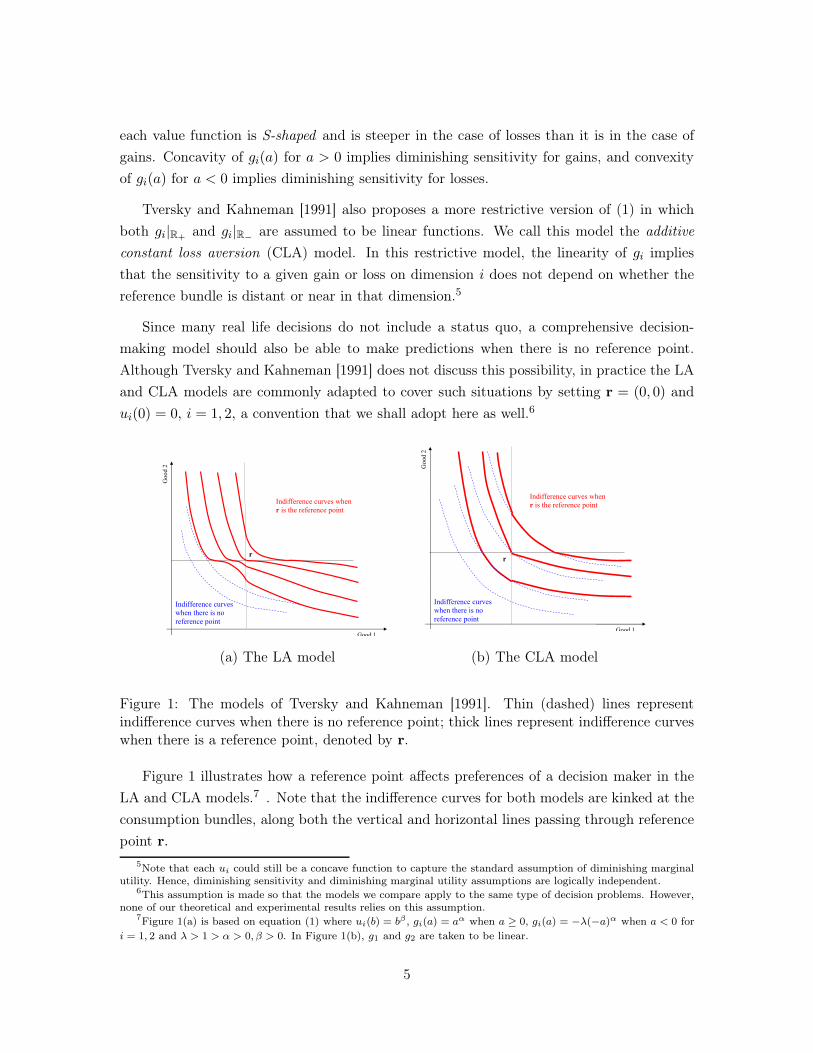
(a) The LA model (b) The CLA model

Figure 1: The models of Tversky and Kahneman [1991]. Thin (dashed) lines representindifference curves when there is no reference point; thick lines represent indifference curveswhen there is a reference point, denoted by r.

Figure 1 illustrates how a reference point affects preferences of a decision maker in the

LA and CLA models.7 . Note that the indifference curves for both models are kinked at the

consumption bundles, along both the vertical and horizontal lines passing through reference

point r.

5Note that each ui could still be a concave function to capture the standard assumption of diminishing marginalutility. Hence, diminishing sensitivity and diminishing marginal utility assumptions are logically independent.

6This assumption is made so that the models we compare apply to the same type of decision problems. However,none of our theoretical and experimental results relies on this assumption.

7Figure 1(a) is based on equation (1) where ui(b) = bβ , gi(a) = aα when a ≥ 0, gi(a) = −λ(−a)α when a < 0 for

i = 1, 2 and λ > 1 > α > 0, β > 0. In Figure 1(b), g1 and g2 are taken to be linear.

5

Köszegi and Rabin [2006] extends the loss aversion model by assuming that individuals

evaluate alternatives not only by comparing them with a reference point but also by consid-

ering the outcomes themselves.8 Formally, Köszegi and Rabin propose the following form of

reference-dependent utility function:

Ur(x) =∑

i

ui(xi) +∑

i

gi(ui(xi)− ui(ri)),

where the first component represents the consumption utility and the second component is

the gain-loss utility. Even though this functional form is different than the LA model, the

effect of moving the reference point on the relative ranking of two alternatives is the same

for both of these models. Hence for convenience we only focus on the LA model in this

paper.

2.1.2 Status Quo Constraint Models

Reference dependence has been commonly treated as a violation of rationality in the liter-

ature on consumer choice. Recently, however, Masatlioglu and Ok [2005, 2007, 2010] has

brought a new perspective on modeling reference dependence.9 In these models, as opposed

to the earlier approach, status quo does not affect the underlying utility function of the agent

but instead imposes a psychological constraint on what the decision maker can choose.

The model of Masatlioglu and Ok [2005]—hereafter referred to as the Status Quo Bias

(SQB) model—is derived through behavioral axioms, in the tradition of the classical revealed

preference theory. In particular, the primary descriptive axiom of Masatlioglu and Ok [2005]

is “status quo bias,” which says that an alternative is more likely to be chosen when it is

the default option of a decision maker. While the SQB model applies in any arbitrary finite

choice space X, one can easily extend this model to uncountable spaces (such as R2) by

imposing an appropriate continuity assumption. For comparison purposes, here the set of

all alternatives is assumed to be R2.

There are two main components of this model: (i) the reference point imposes a men-

tal constraint, and hence, some alternatives are discarded by the decision maker; (ii) the

final decision is made according to a reference-independent utility function from surviving

alternatives.

One of the interpretations of the model is that the decision maker has multiple selves,

8Another innovation of this paper is to introduce a theory of endogenous reference points. Since in our paper we

consider exogenously given reference points, this feature of the model is irrelevant.9See Tapki [2007], Kawai [2008], Houy [2007] for extensions and variations of this model.

6

say two selves, 1 and 2. While self 1 values the first attribute more than the second one, self

2 puts more weight on the second attribute relative to the first one. Each self has a utility

function (say u1 and u2).10 The decision maker sticks to her status quo unless both selves

are willing to move away from it. Put differently, if an alternative, say x, provides higher

utilities for both self 1 and self 2, then both selves agree that x is better than the status

quo. Consequently, we define the set Q(r) as the set of alternatives that are preferred by

both selves when r is the reference point. Formally,

Q(r) = {x ∈ R2| u1(x) ≥ u1(r) and u2(x) ≥ u2(r)}.11 (2)

If there are multiple feasible alternatives belonging to this set, the decision maker maximizes

an aggregation of these utility functions of the two selves, U = w1u1+w2u2, where wi is the

weight assigned to the utility of self i.12 This is the reference-independent utility function. If

there is no reference point, the decision maker solves her problem by maximizing her utility

function over all feasible alternatives.

Goo

d 2

Good 1

u1

u2

r

Indifference curves when

r is the reference point

Q(r)

Indifference curves

when there is no

reference point

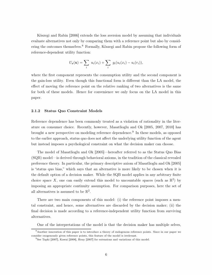
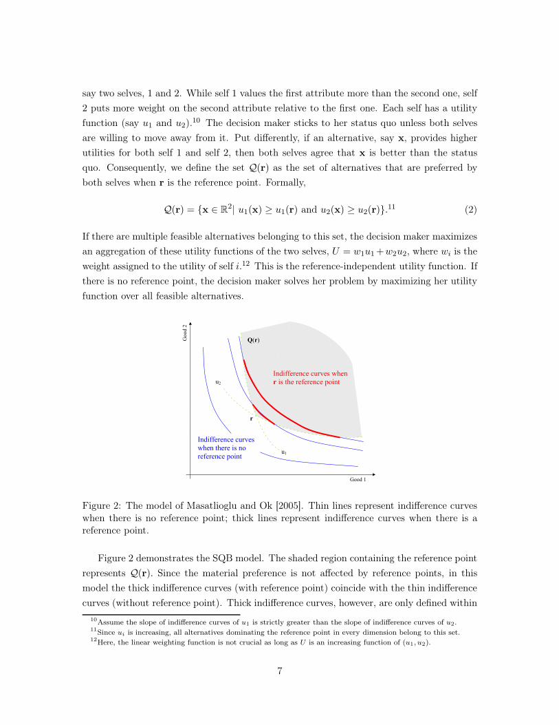
Figure 2: The model of Masatlioglu and Ok [2005]. Thin lines represent indifference curveswhen there is no reference point; thick lines represent indifference curves when there is areference point.

Figure 2 demonstrates the SQB model. The shaded region containing the reference point

represents Q(r). Since the material preference is not affected by reference points, in this

model the thick indifference curves (with reference point) coincide with the thin indifference

curves (without reference point). Thick indifference curves, however, are only defined within

10Assume the slope of indifference curves of u1 is strictly greater than the slope of indifference curves of u2.11Since ui is increasing, all alternatives dominating the reference point in every dimension belong to this set.12Here, the linear weighting function is not crucial as long as U is an increasing function of (u1, u2).

7

the mental constraint set, Q, since any point outside of this set is dominated by the reference

point.

Essentially, in this model, the decision maker maximizes her utility function subject to a

psychological constraint imposed by the status quo. In particular, agents solve the following

maximization problem given budget set B:

max w1u1(x) + w2u2(x)

s.t. x ∈ B ∩Q(r),(3)

where Q(r) = {x ∈ R2| u1(x) ≥ u1(r) and u2(x) ≥ u2(r)}.

The formulation above elucidates that the SQB model is a “constrained utility maximiza-

tion model,” where the constraint set, Q, is induced by one’s reference point. The mental

constraint set consists of alternatives for which the decision maker is willing to abandon her

status quo r.

The mental constraint set satisfies the following properties: (i) strict improvement : if

someone prefers an alternative to the status quo, such an alternative must yield strictly

higher utility to the agent (if x ∈ Q(r)\{r}, then U(r) < U(x)),13 (ii) attainability of

status quo: the status quo is always feasible, i.e., r ∈ Q(r), and (iii) monotonicity : if r′

is revealed to be better than the status quo (r), then any element that is preferred to r′

when r′ is the status quo must be revealed to be better than r when r is the status quo (i.e.

r′ ∈ Q(r) ⇒ Q(r′) ⊂ Q(r)).

Unlike loss aversion models, the SQB model allows us to construct a ranking of alterna-

tives based on unambiguous comparisons that can be used to carry out a meaningful welfare

analysis. Since the SQB model accommodates behavioral anomalies, we cannot summarize

status quo bias choices with a consistent preference ordering as in classical choice theory.

Nevertheless, the existence of a transitive (not necessarily complete) ranking is guaranteed

by the SQB model for welfare comparison purposes.14

Masatlioglu and Ok [2007, 2010] have recently provided two independent extensions of

the SQB model. We refer to the model in Masatlioglu and Ok [2010] as the general SQB

(GSQB) model and the model in Masatlioglu and Ok [2007] as the procedural reference-

13This property prevents potential cycles: if x is chosen in some budget set when y is the status quo, U(y) < U(x),

and z is chosen in some budget set when x is the status quo, U(x) < U(z), then it is impossible that y is chosen in

any budget set when z is the status quo. Indeed, this argument also works for weak improvements.14 To see this, define a “welfare” ranking in the following way: x is “strictly better” than y (x ≻ y) if and only

if x is uniquely chosen from {x,y} when y is the status quo. The SQB model implies that there is no alternative z

such that y is chosen from {x,y, z} when z is the status quo. Hence, independent of status quo, x ≻ y entails that

whenever x and y are available, either x is chosen but not y or neither are chosen. Property (iii) guarantees that ≻

is transitive. Therefore, ≻ can be used for welfare comparisons.

8

dependent choice (PRD) model. We will discuss them in turn.15

The GSQB model operates similarly to the SQB model, except that the mental constraint

set might not have the multiple-self interpretation. Formally, the decision maker solves the

following maximization problem given budget set B:

max U(x)

s.t. x ∈ B ∩Q(r).(4)

The GSQB model satisfies (i) weak improvement : if x ∈ Q(r)\{r}, then U(r) ≤ U(x)

and (ii) attainability of status quo. In addition, since the choice space is endowed with

an order structure, as in R2, it is natural to assume that an alternative that dominates

another alternative in every dimension should have higher utility value. Moreover, if an

alternative dominates the reference point in every dimension, it is unambiguously better

than the reference point; hence, this alternative should be in the mental constraint set.

That is, {x ∈ R2| x1 ≥ r1 and x2 ≥ r2} ⊆ Q(r).

The important difference between the GSQB model and the SQB model is that the

mental constraint set does not satisfy the monotonicity property (r′ ∈ Q(r) implies Q(r′) ⊂Q(r)). After discarding this condition, the GSQB model enjoys more explanatory power

than the SQB model.

The PRD model also resembles the SQB model, yet it functions through two nested

mental constraint sets Q1(r) and Q2(r) for a given reference point, r, such that Q1(r) ⊂Q2(r). In the elimination stage, either Q1 or Q2 will be utilized and Q1 has a priority. If

B ∩ Q1(r) 6= {r}, then she proceeds to the optimization stage, as in the SQB model. If

there is no common element in B and Q1(r) other than r, then the decision maker relaxes

her mental constraint set to a larger set Q2(r) and employs Q2(r) in the elimination stage.

Therefore, at the optimization stage, if B ∩ Q1(r) 6= {r}, the decision maker settles her

problem by selecting alternatives in B ∩Q1(r); otherwise she selects from B ∩Q2(r). More

formally, the optimization problem of the decision maker in the PRD model can be written

as follows:

max U(x)

s.t.

{

x ∈ B ∩ Q1(r)

x ∈ B ∩ Q2(r)

if B ∩Q1(r) 6= {r}otherwise.

(5)

15Dean [2008] challenges both loss aversion and status quo constraint models. Dean finds that status quo is more

frequently chosen when the choice set gets larger (decision avoidance), which cannot be explained by these models.

However, Dean also shows that these models are needed to understand behavior in small choice sets.

9

One can think of Q1(r) as the set of alternatives that dominate the reference point, r,

in an obvious way: no cognitive effort is needed to figure out the domination. In contrast,

Q2(r) consists of those alternatives where the dominance over r is less straightforward: at

least some cognitive work on the part of the individual is needed to discern this dominance.

Both Q1 and Q2 satisfy the three properties of the SQB model, and Q1(r) ⊂ {x ∈ R2| x1 ≥r1 and x2 ≥ r2} ⊆ Q2(r).16

2.2 Behavioral Properties

So far we have reviewed two classes of reference-dependent choice models in a unified manner

and have discussed their natures. The previous section makes apparent how models within

each group relate to one another. We have yet to show how models in the two different

classes are related. To build these connections, we state several properties suggested by

Tversky and Kahneman [1991] and Masatlioglu and Ok [2005, 2007] and study whether

these properties are satisfied by each model. This will allow us not only to understand these

models better but also to design an experiment that can distinguish among them.

Before we state the properties, we introduce some notation. Throughout the paper,

(S, x) denotes a choice problem with a status quo, where the set of available options are S

and the status quo is x ∈ S. If there is no status quo, we use the notation (S, ⋄) to represent

the corresponding choice problem. The choice behavior is denoted by c, which is a mapping

from all choice problems to the set of alternatives.

The first property, Status Quo Bias, is a simple formulation of experimental findings on

reference-dependent choice. The property says that if a decision maker chooses x among

{x, y} when there is no reference point, then x must be chosen when it is the reference point.

Status Quo Bias Property (SQBP): If x ∈ c({x, y}, ⋄) then x ∈ c({x, y}, x).17

Given the large literature on status quo bias, this is a very weak limitation to satisfy

since it only requires the relative ranking of the status quo point to be at least as good as the

case where it is not labeled as the status quo. Among others, Knetsch [1989] provides strong

evidence in favor of the SQBP. The experiment involves two treatments with two options, a

mug and a candy bar. In the first treatment, subjects are asked to choose one of the options

without an initial endowment. The subjects are equally split between selecting these two

options. In the second treatment, one of the options is given as an initial endowment and

16Although the original model does not impose these requirements, given the interpretation of Q1 and Q2, we find

these assumptions to be reasonable when the domain of choices is the set of two-dimensional consumption bundles.17When the choice is unique, we abuse notation and write x = c(S, r) instead of {x} = c(S, r).

10

subjects have the opportunity to exchange their endowment for the other good. Here, the

vast majority of subjects (around 90 percent) keep their endowments regardless of whether

the endowment is a mug or a candy bar.

In order to define the rest of the properties, we need a multi-dimensional commodity

space. For simplicity, we assume two dimensions. First, we fix two consumption bundles

denoted by x and y, which are positioned so that neither dominates the other, i.e., each

has a superior dimension. The following properties concern how choices are affected when

the location of the reference point shifts along one dimension. Reference points are always

dominated by either x or y or both.

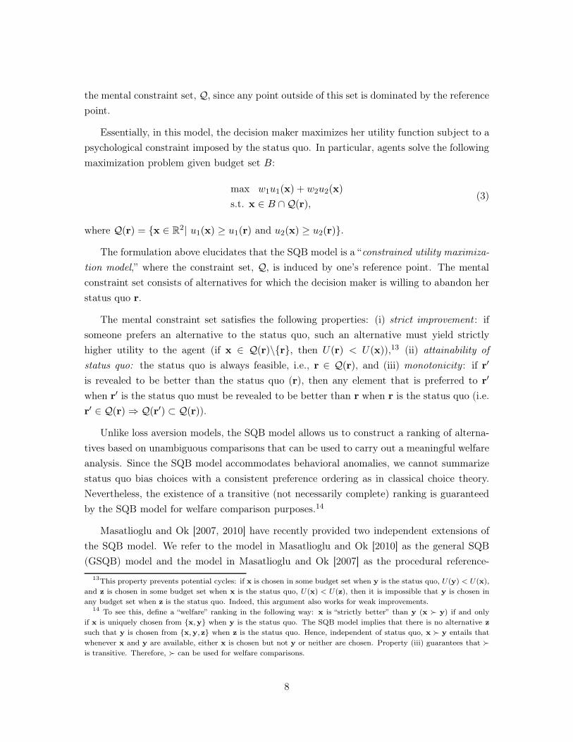
The following properties utilize four pairs of reference points: a− a′, s − s′, l − l′, and

l′− l′′. The a−a′ pair is dominated by y but not by x, hence an asymmetrically dominated

pair. The s − s′ pair is dominated by both y and x, hence a symmetrically dominated

pair. Finally, the l − l′ and l′ − l′′ pairs are dominated by x but not by y (Figure 3). For

simplicity, we will state all the properties in terms of horizontal shifts. Readers should keep

in mind that each property also applies for the vertical shifts, which can be obtained by

interchanging the subscripts 1 and 2 throughout.

y

x

Dimension 1

Dim

ensio

n 2

a`

a

s`

s l` l l``

Figure 3: Reference Point Shifts

The second property we introduce is “Weak Loss Aversion Property”.18

18A similar property is defined by Tversky and Kahneman [1991] under Loss Aversion. We prefer to call this Weak

Loss Aversion since it applies to a boundary case where the shift introduces a loss for y.

11

Weak Loss Aversion Property (WLAP): Suppose x1 ≥ l′1 > l1 = y1 and

y2 > x2 > l2 = l′2. Then x ∈ c({x,y, l}, l) implies x ∈ c({x,y, l′}, l′).

This property captures the basic intuition that “losses loom larger than gains.” Consider

a shift in the reference point from l to l′ (Figure 3). Here, x’s gain with respect to the

reference point is decreased by exactly the same amount as y’s loss is increased. Since losses

are weighted more heavily than gains, the relative attractiveness of y is diminished. Hence,

the effect of the reference shift must be positive for x. In sum, if x is chosen initially, it must

be chosen when l′ is the reference point. This property does not rule out the possibility that y

is initially chosen and then x is chosen after the shift. It rules out the case where x is initially

chosen but y is uniquely chosen after the shift: x ∈ c({x,y, l}, l) and y = c({x,y, l′}, l′).

Notice that y incurs no losses when the reference point is l. Hence, the l → l′ shift

introduces a loss for y. The Strong Loss Aversion Property considers l′ → l′′ shifts where

choosing y at the initial reference point implies some losses, and the reference shift induces

additional losses. The requirement that l1 = y1 is replaced by l′1 > y1, but the same intuition

applies.

Strong Loss Aversion Property (SLAP): Suppose x1 ≥ l′′1 > l′1 > y1 and

y2 > x2 > l′2 = l′′2 . Then x ∈ c({x,y, l′}, l′) implies x ∈ c({x,y, l′′}, l′′).

The fourth property, Irrelevance of Symmetrically Dominated Reference Points, considers

cases where reference points s and s′ are dominated by both x and y. The property says

that individual choice should not be affected by a shift in the reference point from s to

s′. Indeed, any shift in this region—including a shift from the origin—does not have any

impact on choices. This property captures the idea that a reference shift has an effect on

choices only when it makes one of the alternatives more desirable or salient than the other

alternative.

Irrelevance of Symmetrically Dominated Reference Points (ISD):

If x1 > y1 ≥ s′1 > s1 and y2 > x2 ≥ s2 = s′2, then c({x,y, s}, s) = c({x,y, s′}, s′).19

The next property, Irrelevance of Asymmetrically Dominated Reference Points, is similar

to ISD but applies to asymmetrically dominated reference points. That is, both reference

points, a and a′, are dominated by y, but not x (Figure 3). The property implies that the

choices are not affected by moving the reference point from a to a′. Note that while the

19Both Tversky and Kahneman [1991] and Masatlioglu and Ok [2010] provide a similar property under the name

“sign dependence” and “status quo irrelevance”, respectively.

12

location of asymmetrically dominated reference points does not matter, this property allows

choices to be affected by the existence of asymmetrically dominated reference points.

Irrelevance of Asymmetrically Dominated Reference Points (IAD):

If x1 > y1 ≥ a′1 > a1 and y2 ≥ a2 = a′2 > x2, then c({x,y,a},a) = c({x,y,a′},a′).

The combination of ISD and IAD is dubbed “constant sensitivity” by Tversky and Kah-

neman [1991]. These two properties imply that there is no choice reversal for the a → a′

and s → s′ shifts. Hence, they have high predictive power. The next two properties replace

constant sensitivity with diminishing sensitivity and allow a certain choice reversal.

Diminishing Sensitivity for Symmetrically Dominated Reference Points

(DSS): If x1 > y1 ≥ s′1 > s1 and y2 > x2 ≥ s2 = s′2, then x ∈ c({x,y, s}, s)implies x = c({x,y, s′}, s′).

Diminishing Sensitivity for Asymmetrically Dominated Reference

Points (DSA): If x1 > y1 ≥ a′1 > a1 and y2 ≥ a2 = a′2 > x2, then x ∈c({x,y,a},a) implies x = c({x,y,a′},a′).

These two properties are conceptually similar to the well-known phenomenon of diminish-

ing marginal utility. Tversky and Kahneman [1991] states that “The marginal value decreases

with the distance from the reference point.” For instance, the marginal value of $1,000 in

addition to a salary of $60,000 is smaller when the current salary is $40,000 than when

it is $55,000. Nevertheless, they are logically different from diminishing marginal utility.

The combination of DSS and DSA is coined “diminishing sensitivity for gains” by Tversky

and Kahneman [1991]. These two properties rule out cases where x is initially chosen at

reference point r and then y is chosen at reference point r′ where (r, r′) ∈ {(a,a′), (s, s′)}.Choice reversal in the opposite direction is allowed: y is chosen from {x,y, r} at r and x is

chosen from {x,y, r′} at r′.

Proposition 1 and 2 provide our main theoretical results. Proofs of the propositions are

provided in Appendix A.

Proposition 1 Let the domain be a two-dimensional commodity space. Then

(i) The CLA model satisfies SQBP, WLAP, SLAP, ISD, and IAD,

(ii) The LA model satisfies WLAP, DSS and DSA.

13

This proposition makes it clear that the CLA model enjoys much higher prediction power

than the LA model. The LA model is not consistent with the predictions of SQBP, SLAP,

ISD and IAD.

Proposition 2 Let the domain be a two-dimensional commodity space. Then

(i) The SQB model satisfies SQBP, WLAP, SLAP, and ISD,

(ii) The GSQB model satisfies SQBP, WLAP, and ISD,

(iii) The PRD model satisfies SQBP.

Within status quo constraint models, the SQB model has much higher prediction power.

The PRD model is only consistent with SQBP.

Table 1: Properties of Reference-Dependent Models Under Consideration

Tversky-Kahneman Masatlioglu-OkCLA LA SQB GSQB PRD

SQBP√ √ √ √

WLAP√ √ √ √

SLAP√ √

ISD√ √ √

IAD√

DSS√

DSA√

Section 3 develops an experimental design that allows us to contrast the loss aversion

models of Tversky and Kahneman with the status quo constraint models of Masatlioglu

and Ok. Not every property is useful for this purpose. First of all, SQBP is not only

well-established but also satisfied by all models except the LA model. Therefore, we have

not included this property in our experiment. While WLAP and SLAP may differentiate

between the special and generalized versions of these models, these are not very helpful

to distinguish between these two groups of models. Finding evidence against these two

properties would show that more general models are needed. However, we will not be able

to judge between the general versions of loss aversion and status quo constraint models.20

On the contrary, a joint test of ISS, IAD, DSS and DSA would help us contrast between

models. By focusing on a → a′ and s → s′ shifts, Section 4 tests which properties are

satisfied. Section 5 shows that these properties only partially identify the predictions of

20An exception to this is finding evidence against WLAP since it is satisfied by all models except PRD. However,since the PRD model does not provide any intuitive reason as to why this property may be violated, we do not expectto see that this property will fail. Hence, we do not consider this property either.

14

different models. When these properties are violated, more needs to be done to figure out

the predictions of each model for each shift. Section 5 is devoted to theoretical predictions

of the models and their explanatory powers.

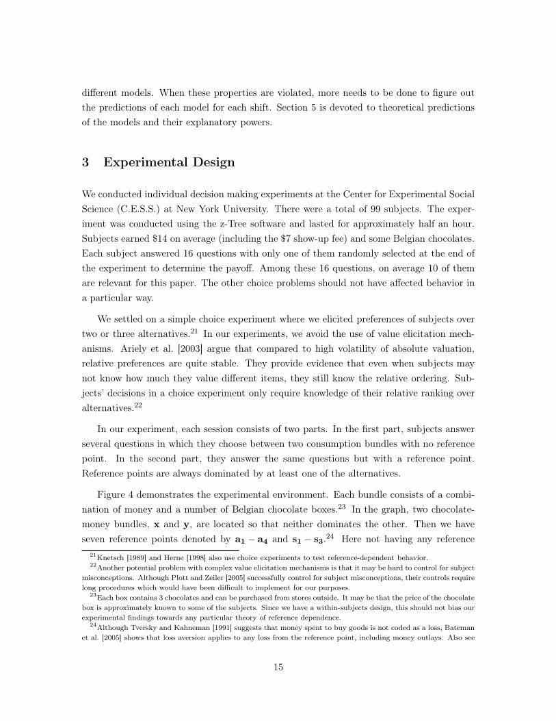
3 Experimental Design

We conducted individual decision making experiments at the Center for Experimental Social

Science (C.E.S.S.) at New York University. There were a total of 99 subjects. The exper-

iment was conducted using the z-Tree software and lasted for approximately half an hour.

Subjects earned $14 on average (including the $7 show-up fee) and some Belgian chocolates.

Each subject answered 16 questions with only one of them randomly selected at the end of

the experiment to determine the payoff. Among these 16 questions, on average 10 of them

are relevant for this paper. The other choice problems should not have affected behavior in

a particular way.

We settled on a simple choice experiment where we elicited preferences of subjects over

two or three alternatives.21 In our experiments, we avoid the use of value elicitation mech-

anisms. Ariely et al. [2003] argue that compared to high volatility of absolute valuation,

relative preferences are quite stable. They provide evidence that even when subjects may

not know how much they value different items, they still know the relative ordering. Sub-

jects’ decisions in a choice experiment only require knowledge of their relative ranking over

alternatives.22

In our experiment, each session consists of two parts. In the first part, subjects answer

several questions in which they choose between two consumption bundles with no reference

point. In the second part, they answer the same questions but with a reference point.

Reference points are always dominated by at least one of the alternatives.

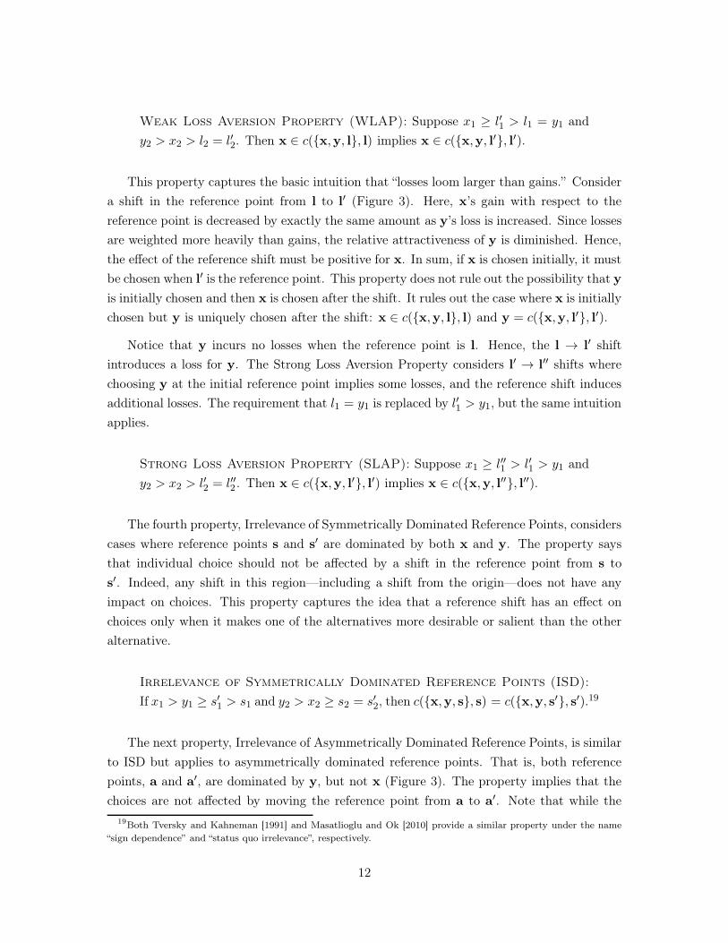
Figure 4 demonstrates the experimental environment. Each bundle consists of a combi-

nation of money and a number of Belgian chocolate boxes.23 In the graph, two chocolate-

money bundles, x and y, are located so that neither dominates the other. Then we have

seven reference points denoted by a1 − a4 and s1 − s3.24 Here not having any reference

21Knetsch [1989] and Herne [1998] also use choice experiments to test reference-dependent behavior.22Another potential problem with complex value elicitation mechanisms is that it may be hard to control for subject

misconceptions. Although Plott and Zeiler [2005] successfully control for subject misconceptions, their controls require

long procedures which would have been difficult to implement for our purposes.23Each box contains 3 chocolates and can be purchased from stores outside. It may be that the price of the chocolate

box is approximately known to some of the subjects. Since we have a within-subjects design, this should not bias our

experimental findings towards any particular theory of reference dependence.24Although Tversky and Kahneman [1991] suggests that money spent to buy goods is not coded as a loss, Bateman

et al. [2005] shows that loss aversion applies to any loss from the reference point, including money outlays. Also see

15

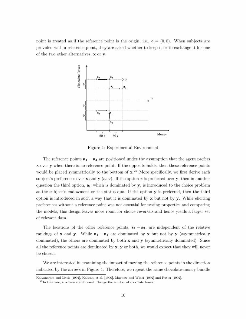
point is treated as if the reference point is the origin, i.e., ⋄ = (0, 0). When subjects are

provided with a reference point, they are asked whether to keep it or to exchange it for one

of the two other alternatives, x or y.

y

x

Money

Ch

oco

late

Bo

xes

a2

a1

s1

s3

a4

a3

s2

1

1

1

60 ¢ 60 ¢

Figure 4: Experimental Environment

The reference points a1 − a4 are positioned under the assumption that the agent prefers

x over y when there is no reference point. If the opposite holds, then these reference points

would be placed symmetrically to the bottom of x.25 More specifically, we first derive each

subject’s preferences over x and y (at ⋄). If the option x is preferred over y, then in another

question the third option, ai, which is dominated by y, is introduced to the choice problem

as the subject’s endowment or the status quo. If the option y is preferred, then the third

option is introduced in such a way that it is dominated by x but not by y. While eliciting

preferences without a reference point was not essential for testing properties and comparing

the models, this design leaves more room for choice reversals and hence yields a larger set

of relevant data.

The locations of the other reference points, s1 − s3, are independent of the relative

rankings of x and y. While a1 − a4 are dominated by x but not by y (asymmetrically

dominated), the others are dominated by both x and y (symmetrically dominated). Since

all the reference points are dominated by x, y or both, we would expect that they will never

be chosen.

We are interested in examining the impact of moving the reference points in the direction

indicated by the arrows in Figure 4. Therefore, we repeat the same chocolate-money bundle

Kalyanaram and Little [1994], Kalwani et al. [1990], Mayhew and Winer [1992] and Putler [1992].25In this case, a reference shift would change the number of chocolate boxes.

16

three times, corresponding to three different reference points, with one being the origin

(no reference point). Note that the x-y pair differs for different reference shifts. In order to

control for possible order effects, we randomize the order of the questions in the experiment.26

One may be concerned that subjects may artificially try to be consistent in their choices.

This would reduce the occurrence of choice reversals and increase the explanatory power of

the standard theory. However, this should not have any effect on the comparison between

the reference-dependent choice models. Moreover, it is unlikely that the subjects remember

their previous choices since these questions are separated from each other and throughout

the experiment, once subjects make their decisions, they cannot go back.

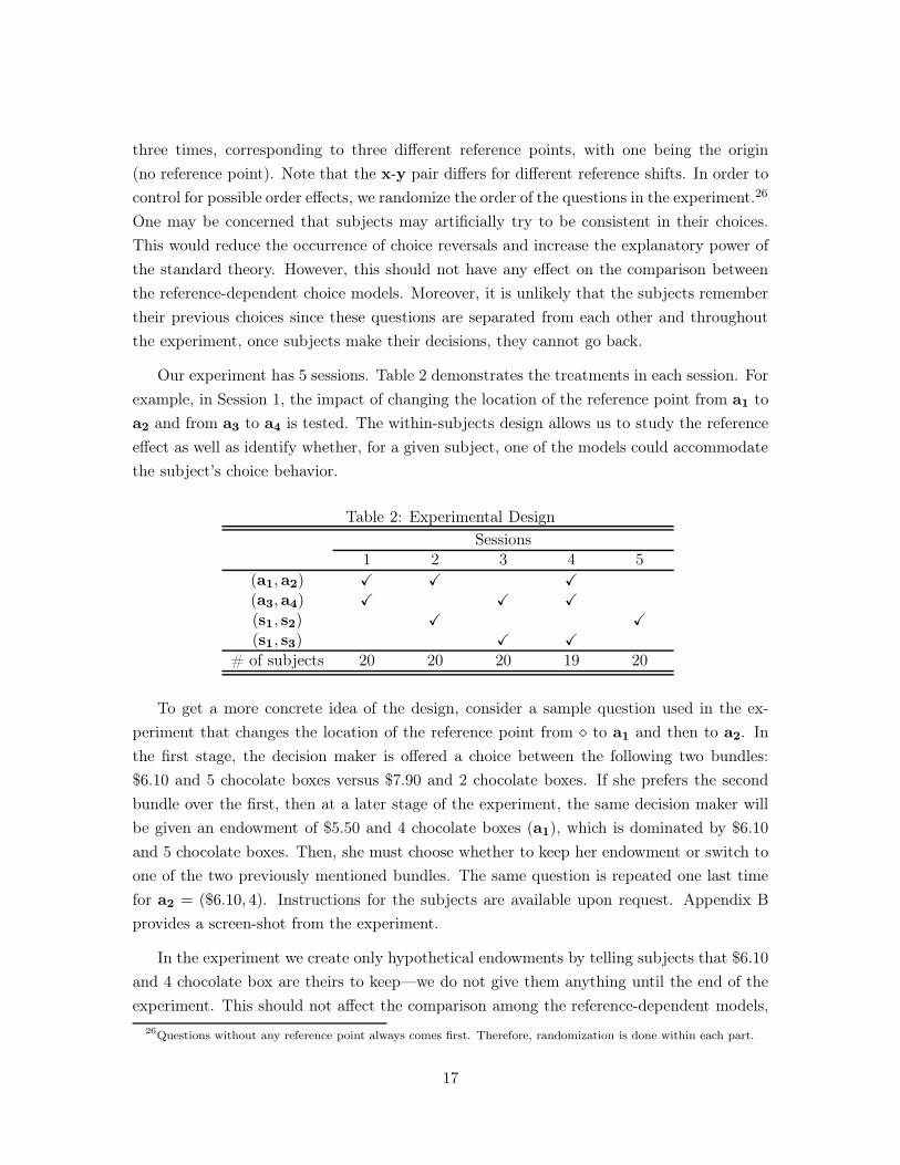
Our experiment has 5 sessions. Table 2 demonstrates the treatments in each session. For

example, in Session 1, the impact of changing the location of the reference point from a1 to

a2 and from a3 to a4 is tested. The within-subjects design allows us to study the reference

effect as well as identify whether, for a given subject, one of the models could accommodate

the subject’s choice behavior.

Table 2: Experimental Design

Sessions1 2 3 4 5

(a1,a2) X X X

(a3,a4) X X X

(s1, s2) X X

(s1, s3) X X

# of subjects 20 20 20 19 20

To get a more concrete idea of the design, consider a sample question used in the ex-

periment that changes the location of the reference point from ⋄ to a1 and then to a2. In

the first stage, the decision maker is offered a choice between the following two bundles:

$6.10 and 5 chocolate boxes versus $7.90 and 2 chocolate boxes. If she prefers the second

bundle over the first, then at a later stage of the experiment, the same decision maker will

be given an endowment of $5.50 and 4 chocolate boxes (a1), which is dominated by $6.10

and 5 chocolate boxes. Then, she must choose whether to keep her endowment or switch to

one of the two previously mentioned bundles. The same question is repeated one last time

for a2 = ($6.10, 4). Instructions for the subjects are available upon request. Appendix B

provides a screen-shot from the experiment.

In the experiment we create only hypothetical endowments by telling subjects that $6.10

and 4 chocolate box are theirs to keep—we do not give them anything until the end of the

experiment. This should not affect the comparison among the reference-dependent models,

26Questions without any reference point always comes first. Therefore, randomization is done within each part.

17

but the reference effect would have been stronger if we had actually endowed them with

bundles.27

We now summarize the implications of each property for each shift shown in Figure 4.

Since the shifts provided here are simply a subset of Figure 3, the implications will be based

on Section 2.2. Before we explain implications, we introduce some notations and definitions.

Given an r1 → r2 shift, 〈a, b〉r1,r2 denotes choices from {x,y, r1} and {x,y, r2} when the

reference point is r1 and r2, respectively. We will omit the subscript if there is no confusion

about the reference shift. Note that there are nine possibilities: 〈x,x〉, 〈x,y〉, 〈x, r2〉, 〈y,x〉,〈y,y〉, 〈y, r2〉, 〈r1,x〉, 〈r1,y〉, and 〈r1, r2〉. Since each reference point is dominated by at

least one other bundle, we expect that the reference points will never be chosen.28 Hence, for

brevity, we focus on four cases: 〈x,x〉, 〈x,y〉, 〈y,x〉, and 〈y,y〉. The following implications

are valid independent of this simplification.

Definition 1 An r1 → r2 shift favors x over y if x must be chosen from {x,y, r2} at r2

whenever an agent chooses x from {x,y, r1} at r1.29 We simply say the r1 → r2 shift favors

x if there is no confusion about y.

Definition 2 A subject exhibits a choice reversal at r if the subject makes different choices

with and without the reference point r.

Consider an s2 → s1 shift. Since DSS states that a shift from s2 to s1 favors y (the

bundle with more chocolate), the possibility of 〈y,x〉 is eliminated, but 〈x,x〉, 〈y,y〉, 〈x,y〉are still possible. Similarly, an s3 → s1 shift favors x (the bundle with more money). We

now list the implications of the properties (see Table 3).

Implication 1. Under DSS, the number of subjects who pick the option with more

chocolate (y) will be weakly higher at s1 compared to s2 and the number of subjects who

pick the option with more money (x) will be higher at s1 compared to s3.

On the other hand, ISD restricts the possible outcomes to 〈x,x〉 and 〈y,y〉. Thus, it

imposes no change in the number of choice reversals in aggregate.

Implication 2. Under ISD, there will be no change in the number of subjects choosing

option (x) over (y) when the reference points are dominated by both alternatives.

27Loewenstein and Adler [1995] show that hypothetical ownership creates less endowment effect. However, this

does not mean that hypothetical ownership does not create reference-dependence. In Section 6, we argue that a status

quo, with hypothetical ownership, has a stronger impact on individual choice behavior compared to a decoy option,

where a decoy option is introduced without imposing an ownership.28Indeed, there are only three observations out of 394 where a dominated reference point is chosen.29Since constraint choice models use a revealed preference approach, we define this over choices and not over

preferences.

18

Table 3: Implications of Properties

Initial Choicex y

s2 → s1ISD no change no changeDSS more y more y

s3 → s1ISD no change no changeDSS more x more x

a1 → a2and

a3 → a4

IAD no change no change

DSAmore x more y

(less choice reversals) (less choice reversals)

The positions of a1 − a4 depend on the initial choice between x and y, where x is the

bundle that has more money and y is the bundle that has more chocolate boxes. We will

translate the predictions of IAD and DSA in terms of choice reversals so that they will not

depend on the initial choice when there is no reference point.30

Assume the subject’s initial choice is x when there is no reference point. Consider an

a1 → a2 shift. Since DSA states that a shift from a1 to a2 favors x (the bundle with more

money), the possibility of 〈x,y〉 is eliminated but 〈x,x〉, 〈y,y〉, 〈y,x〉 are still possible. In

other words, an agent cannot exhibit a choice reversal at a2 if there has not been a choice

reversal at a1.

Now, consider the initial choice is y when there is no reference point. Since DSA states

that a shift from a1 to a2 favors y (the bundle with more chocolate boxes), the possibility

of 〈y,x〉 is eliminated but 〈x,x〉, 〈y,y〉, 〈x,y〉 are still possible. Thus, if the subject exhibits

a choice reversal at a2, she must exhibit a choice reversal at a1.

In conclusion, the subject’s choice behavior is consistent with DSA if she exhibits the

same amount or fewer choice reversals at a2 than at a1, independent of the initial choice.

In the aggregate, the number of subjects who exhibit choice reversals at a2 is less than the

number of subjects who exhibit choice reversals at a1. The same applies for a shift from a3

to a4.

Implication 3. Under DSA, the number of subjects who exhibit choice reversals at a2

(a4) is weakly less than the number of subjects who exhibit choice reversals at a1 (a3).

30By pooling our data across cases in which the subjects initially chose the option with more money and those in

which they initially chose the option with more chocolate, we are able to increase our power for statistical testing. In

our experiment, subjects are more likely to choose the option with more money. Moreover, we observe that reference

effect is lower for subjects who pick the option with more money initially. In other words, subjects who initially

pick the option with more money demonstrate fewer choice reversals. However, this should not affect the qualitative

comparison of the models.

19

On the other hand, IAD restricts the possible outcomes to 〈x,x〉 and 〈y,y〉, indepen-

dent of the initial choice. Thus, it imposes no change in the number of choice reversals in

aggregate.

Implication 4. Under IAD, there is no change in the number of subjects who exhibit

choice reversals at a2 (a4) versus at a1 (a3).

Before we move to the next section, we point out that in the case where a subject is indif-

ferent or makes mistakes, Implications 1-4 continue to hold even under such circumstances,

as we do not expect to see any particular direction of bias.

4 Experimental Results

In this section, we analyze how the reference effect operates and if it depends on the location

of the reference points. In particular, we compare two regions: asymmetrically dominated

and symmetrically dominated reference points. This will help us identify whether the data

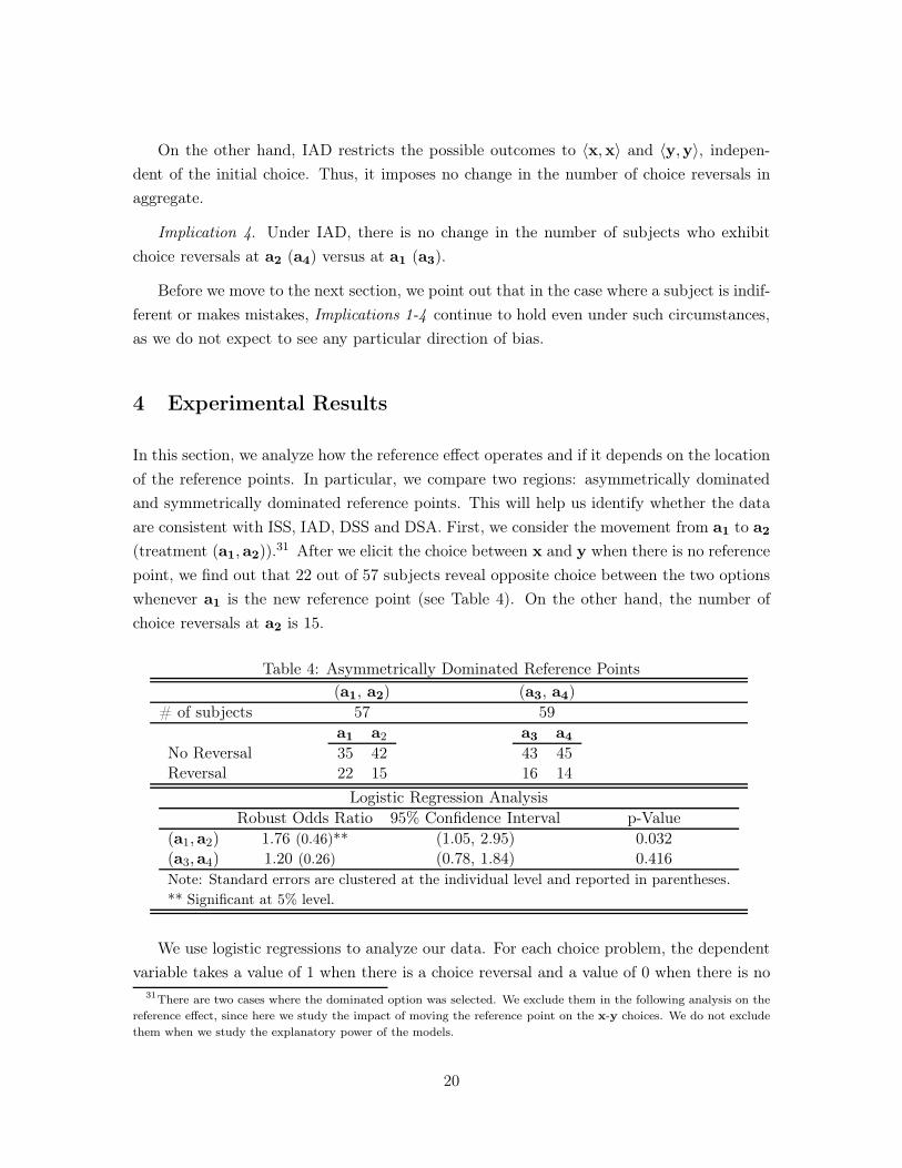
are consistent with ISS, IAD, DSS and DSA. First, we consider the movement from a1 to a2

(treatment (a1,a2)).31 After we elicit the choice between x and y when there is no reference

point, we find out that 22 out of 57 subjects reveal opposite choice between the two options

whenever a1 is the new reference point (see Table 4). On the other hand, the number of

choice reversals at a2 is 15.

Table 4: Asymmetrically Dominated Reference Points

(a1, a2) (a3, a4)

# of subjects 57 59

No ReversalReversal

a1 a2

35 4222 15

a3 a4

43 4516 14

Logistic Regression Analysis

Robust Odds Ratio 95% Confidence Interval p-Value

(a1,a2) 1.76 (0.46)** (1.05, 2.95) 0.032(a3,a4) 1.20 (0.26) (0.78, 1.84) 0.416

Note: Standard errors are clustered at the individual level and reported in parentheses.

** Significant at 5% level.

We use logistic regressions to analyze our data. For each choice problem, the dependent

variable takes a value of 1 when there is a choice reversal and a value of 0 when there is no

31There are two cases where the dominated option was selected. We exclude them in the following analysis on the

reference effect, since here we study the impact of moving the reference point on the x-y choices. We do not exclude

them when we study the explanatory power of the models.

20

change in a subject’s choice. The independent variable is also a binary variable. It takes a

value of 1 if the reference point is a1 and 0 if the reference point is a2. Table 4 also presents

the regression results. Logistic regression analysis shows that the odds of a choice reversal

is 1.76 times greater when the reference point is a1 compared to a2.

One might argue that choice reversal from one option to the other can simply be at-

tributed to subjects being indifferent between these two options, or that subjects may be

making a mistake, and not due to the reference effect. Our analysis of moving the location

of the reference point controls for that. If our results were driven by the indifference or error

arguments, then we should have observed no statistically significant difference in the number

of choice reversals at a1 and a2. In contrast, our analysis shows that we can strongly reject

the hypothesis that the number of choice reversals are the same: subjects are more likely to

choose an option when it dominates the reference point in both components.

When the location of the reference point is moved from a3 to a4, we find that 16 and

14 subjects out of 59 switch their decisions at a3 and a4, respectively. Although there are

more choice reversals at a3, this difference is not significant (p = 0.416).

We also pool the data on asymmetrically dominated reference points to check whether

the odds ratio in treatment (a1,a2) is significantly different than the odds ratio in treatment

(a3,a4). We find that a shift in the asymmetrically dominated reference point (a1 to a2, or

a3 to a4) increases the odds of choice reversal by a factor of 1.46 (p = 0.032) and that there

is no significant difference between (a1,a2) and (a3,a4) movements (p = 0.264).

This finding is consistent with diminishing sensitivity for asymmetrically dominated

reference points (DSA). Hence, IAD is violated.

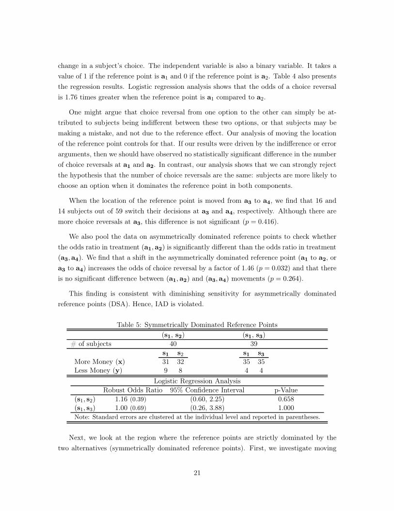
Table 5: Symmetrically Dominated Reference Points

(s1, s2) (s1, s3)

# of subjects 40 39

More Money (x)Less Money (y)

s1 s2

31 329 8

s1 s3

35 354 4

Logistic Regression Analysis

Robust Odds Ratio 95% Confidence Interval p-Value

(s1, s2) 1.16 (0.39) (0.60, 2.25) 0.658(s1, s3) 1.00 (0.69) (0.26, 3.88) 1.000

Note: Standard errors are clustered at the individual level and reported in parentheses.

Next, we look at the region where the reference points are strictly dominated by the

two alternatives (symmetrically dominated reference points). First, we investigate moving

21

the reference point from s2 to s1 (treatment (s1, s2)). At s1 there are 9 subjects (out of

40) who choose the option with more chocolate. The total number of subjects who choose

the option with more chocolate is 8 when the reference point is s2. We cannot reject the

hypothesis that preferences do not change when the reference points are dominated by both

alternatives (p = 0.658).32 Similarly we look at switching the reference point from s3 to s1

(treatment (s1, s3)). Out of 39 people, 35 people choose the option with more money at s1.

Even though a small portion of subjects change their choice when the reference point is s3,

the total number of subjects who choose the option with more money does not change with

moving the reference point (Table 5). Similarly logistic regression analysis shows that the

odds of choosing the option with more chocolate does not change between s1 and s3 (Table

5). We find that our data are consistent with ISD. While one cannot rule out DSS either, it

would be reasonable to argue that DSS is a redundant property given that ISD, a stronger

property with high prediction power, captures the choice behavior.

Our results show that moving the reference point affects individual choices even when

the reference point itself is not chosen. However, we only observe the reference effect for

asymmetrically dominated reference points—in particular when there is a salient dominance

by one option but not the other. We do not see a reference effect for symmetrically dominated

reference points. Hence, we find that both DSA and ISD are desirable properties. However,

there is no single model satisfying both of them at the same time. While the CLA, SQB

and the GSQB models satisfy ISD, the LA model satisfies DSA.

At this point further investigation is needed to compare the performances of these models.

Proposition 1 and 2 only partially identify what each model predicts under different reference

point shifts. For example, the SQB model does not satisfies IAD, but we would like to know

what type of prediction this model makes when the reference points are asymmetrically

dominated. This will allow us to determine the explanatory power of the models. The next

section investigates the predictions and explanatory power of each model.

5 Comparing Models

To compare the models under consideration, we now discuss the predictions of each model

for different reference shifts.

32Note that the dependent variable is now defined as 1 when a subject chooses the alternative with more money

and 0 otherwise.

22

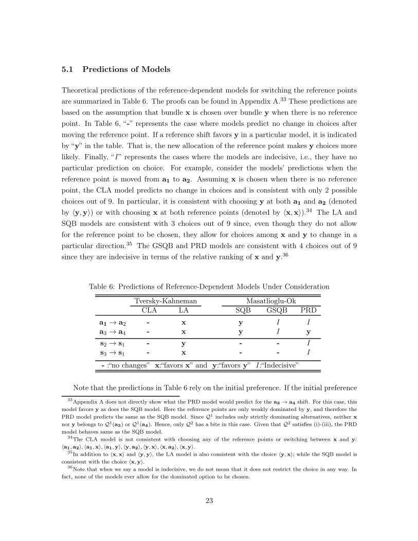
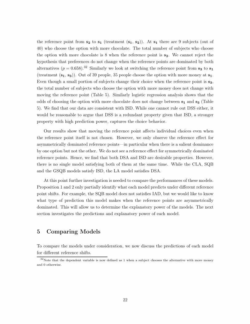
5.1 Predictions of Models

Theoretical predictions of the reference-dependent models for switching the reference points

are summarized in Table 6. The proofs can be found in Appendix A.33 These predictions are

based on the assumption that bundle x is chosen over bundle y when there is no reference

point. In Table 6, “-” represents the case where models predict no change in choices after

moving the reference point. If a reference shift favors y in a particular model, it is indicated

by “y” in the table. That is, the new allocation of the reference point makes y choices more

likely. Finally, “I ” represents the cases where the models are indecisive, i.e., they have no

particular prediction on choice. For example, consider the models’ predictions when the

reference point is moved from a1 to a2. Assuming x is chosen when there is no reference

point, the CLA model predicts no change in choices and is consistent with only 2 possible

choices out of 9. In particular, it is consistent with choosing y at both a1 and a2 (denoted

by 〈y,y〉) or with choosing x at both reference points (denoted by 〈x,x〉).34 The LA and

SQB models are consistent with 3 choices out of 9 since, even though they do not allow

for the reference point to be chosen, they allow for choices among x and y to change in a

particular direction.35 The GSQB and PRD models are consistent with 4 choices out of 9

since they are indecisive in terms of the relative ranking of x and y.36

Table 6: Predictions of Reference-Dependent Models Under Consideration

Tversky-Kahneman Masatlioglu-OkCLA LA SQB GSQB PRD

a1 → a2 - x y I Ia3 → a4 - x y I y

s2 → s1 - y - - Is3 → s1 - x - - I

- :“no changes” x:“favors x” and y:“favors y” I :“Indecisive”

Note that the predictions in Table 6 rely on the initial preference. If the initial preference

33Appendix A does not directly show what the PRD model would predict for the a3 → a4 shift. For this case, this

model favors y as does the SQB model. Here the reference points are only weakly dominated by y, and therefore the

PRD model predicts the same as the SQB model. Since Q1 includes only strictly dominating alternatives, neither x

nor y belongs to Q1(a3) or Q1(a4). Hence, only Q2 has a bite in this case. Given that Q2 satisfies (i)-(iii), the PRD

model behaves same as the SQB model.34The CLA model is not consistent with choosing any of the reference points or switching between x and y:

〈a1,a2〉, 〈a1,x〉, 〈a1,y〉, 〈y, a2〉, 〈y,x〉, 〈x, a2〉, 〈x,y〉.35In addition to 〈x,x〉 and 〈y,y〉, the LA model is also consistent with the choice 〈y,x〉; while the SQB model is

consistent with the choice 〈x,y〉.36Note that when we say a model is indecisive, we do not mean that it does not restrict the choice in any way. In

fact, none of the models ever allow for the dominated option to be chosen.

23

between x and y is y, then the reference points would be placed at the bottom of option x

in a symmetric fashion. Hence, for example, the shift from a1 to a2 would now favor y for

the LA model and x in the SQB model.

5.2 Explanatory Power of the Models

We investigate the relative performance of the models assuming subjects are not indifferent

and do not make mistakes in their choices. Naturally if one allows for subjects being indiffer-

ent between options and errors, then any one of these theories would explain all individual

choices perfectly. Therefore, the question is, while being able to make some predictions,

is there a model that can also accommodate our data? We first study which models can

explain our data. Then, we consider the explanatory power and predictive power of these

models at the same time to provide a more natural comparison.

First, we explore to what extent the classical choice theory can accommodate our exper-

imental data. To do this, we examine how many individuals behave in a manner consistent

with classical choice theory. Remember that each person is going through different treat-

ments (Table 2). We say an individual is consistent with the classical choice theory if her

choices are consistent with this theory at all times (approximately 4 times). For example,

if we see choice reversals at a1 compared to her choice with no reference point, then we say

this individual displays a choice pattern inconsistent with the classical choice theory.37

We find that 42% of all subjects exhibit some reference dependence. Put differently,

roughly half of the time, we observe behavioral patterns inconsistent with the classical choice

theory. Plott and Zeiler [2005, 2007] argue that the endowment effect is driven by subjects’

misconceptions and experimental procedures. In our experiment, we provide a simple choice

environment in which individual choices appear to be influenced by the reference points,

even when the subjects do not stick with the reference point. In other words, reference

dependence is not confined to the endowment effect or status quo bias in general.38

Now, we focus our attention on reference-dependent models. Similarly, we say an indi-

vidual is accommodated by a particular theory if her choices are consistent with this theory

at all times. For example, a subject’s choice behavior cannot be explained by the CLA and

37While classical choice theory predicts that reference points do not affect the relative ranking of x and y, all the

reference-dependent models allow for a change in the relative ranking of alternatives when a reference point a1 − a4

is added to the choice problem. However, models of reference dependence make different predictions when a reference

point s1 − s3 is added to the choice problem. When a reference point is dominated by both alternatives, the CLA,

SQB, and GSQB models predict no preference reversal – the decision maker should stick with her earlier choice. On

the other hand, the other models do not make any particular predictions in this type of situation.38List [2003, 2004] show the endowment effect disappears if subjects have prior experience in trading environments.

Although the reference effect may also diminish with experience, we believe that many real life choices are madewithout much experience.

24

SQB models if the subject displays a preference reversal at a1 but not at a2. This choice

behavior is, nevertheless, consistent with the LA, GSQB, and PRD models (see Table 6).

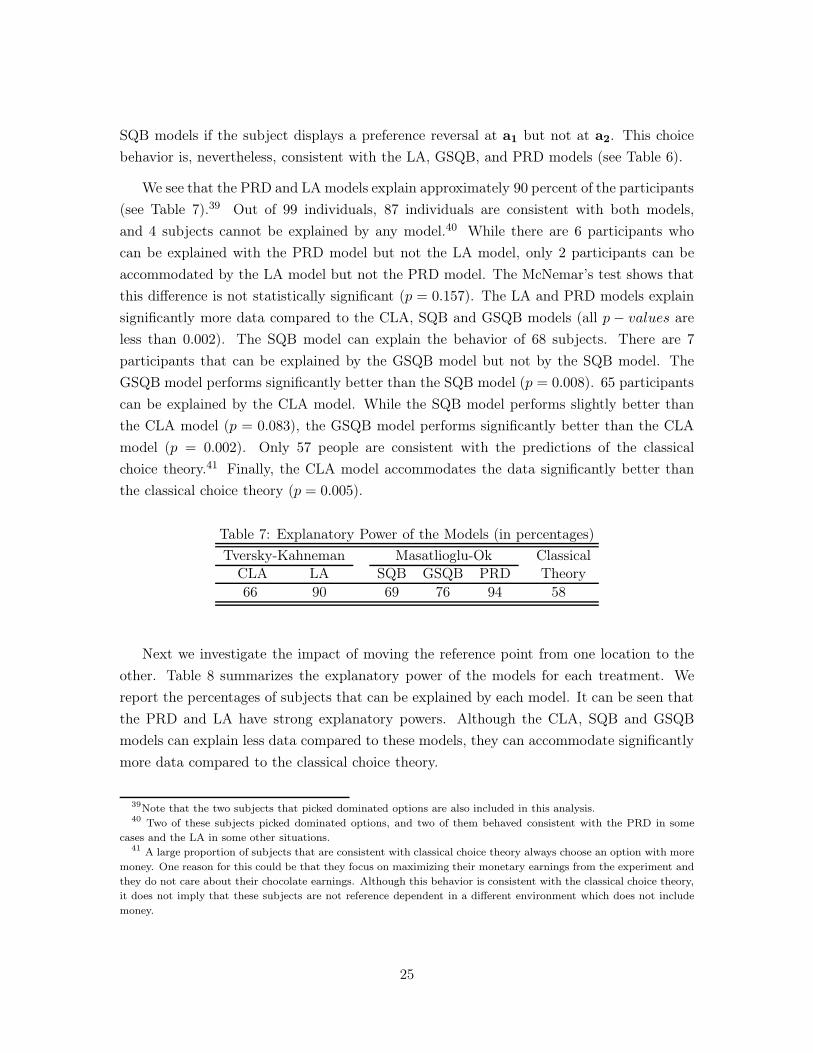
We see that the PRD and LA models explain approximately 90 percent of the participants

(see Table 7).39 Out of 99 individuals, 87 individuals are consistent with both models,

and 4 subjects cannot be explained by any model.40 While there are 6 participants who

can be explained with the PRD model but not the LA model, only 2 participants can be

accommodated by the LA model but not the PRD model. The McNemar’s test shows that

this difference is not statistically significant (p = 0.157). The LA and PRD models explain

significantly more data compared to the CLA, SQB and GSQB models (all p − values are

less than 0.002). The SQB model can explain the behavior of 68 subjects. There are 7

participants that can be explained by the GSQB model but not by the SQB model. The

GSQB model performs significantly better than the SQB model (p = 0.008). 65 participants

can be explained by the CLA model. While the SQB model performs slightly better than

the CLA model (p = 0.083), the GSQB model performs significantly better than the CLA

model (p = 0.002). Only 57 people are consistent with the predictions of the classical

choice theory.41 Finally, the CLA model accommodates the data significantly better than

the classical choice theory (p = 0.005).

Table 7: Explanatory Power of the Models (in percentages)

Tversky-Kahneman Masatlioglu-Ok ClassicalCLA LA SQB GSQB PRD Theory

66 90 69 76 94 58

Next we investigate the impact of moving the reference point from one location to the

other. Table 8 summarizes the explanatory power of the models for each treatment. We

report the percentages of subjects that can be explained by each model. It can be seen that

the PRD and LA have strong explanatory powers. Although the CLA, SQB and GSQB

models can explain less data compared to these models, they can accommodate significantly

more data compared to the classical choice theory.

39Note that the two subjects that picked dominated options are also included in this analysis.40 Two of these subjects picked dominated options, and two of them behaved consistent with the PRD in some

cases and the LA in some other situations.41 A large proportion of subjects that are consistent with classical choice theory always choose an option with more

money. One reason for this could be that they focus on maximizing their monetary earnings from the experiment and

they do not care about their chocolate earnings. Although this behavior is consistent with the classical choice theory,

it does not imply that these subjects are not reference dependent in a different environment which does not include

money.

25

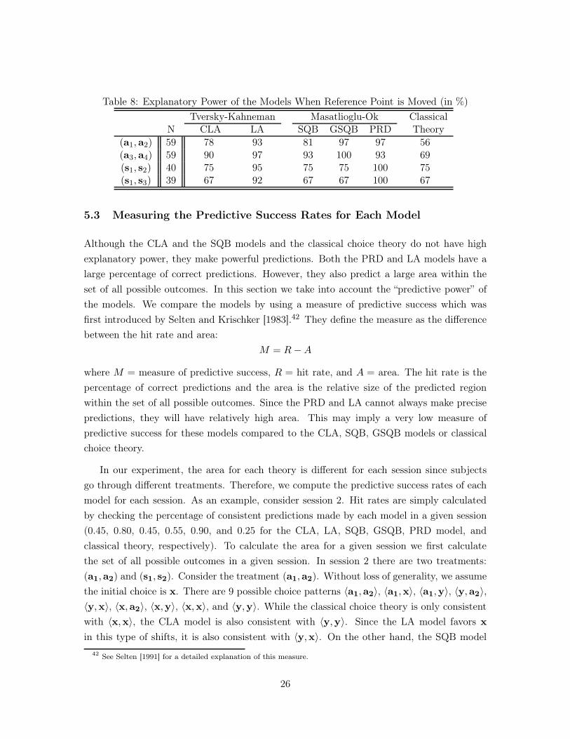
Table 8: Explanatory Power of the Models When Reference Point is Moved (in %)

Tversky-Kahneman Masatlioglu-Ok ClassicalN CLA LA SQB GSQB PRD Theory

(a1,a2) 59 78 93 81 97 97 56(a3,a4) 59 90 97 93 100 93 69(s1, s2) 40 75 95 75 75 100 75(s1, s3) 39 67 92 67 67 100 67

5.3 Measuring the Predictive Success Rates for Each Model

Although the CLA and the SQB models and the classical choice theory do not have high

explanatory power, they make powerful predictions. Both the PRD and LA models have a

large percentage of correct predictions. However, they also predict a large area within the

set of all possible outcomes. In this section we take into account the “predictive power” of

the models. We compare the models by using a measure of predictive success which was

first introduced by Selten and Krischker [1983].42 They define the measure as the difference

between the hit rate and area:

M = R−A

where M = measure of predictive success, R = hit rate, and A = area. The hit rate is the

percentage of correct predictions and the area is the relative size of the predicted region

within the set of all possible outcomes. Since the PRD and LA cannot always make precise

predictions, they will have relatively high area. This may imply a very low measure of

predictive success for these models compared to the CLA, SQB, GSQB models or classical

choice theory.

In our experiment, the area for each theory is different for each session since subjects

go through different treatments. Therefore, we compute the predictive success rates of each

model for each session. As an example, consider session 2. Hit rates are simply calculated

by checking the percentage of consistent predictions made by each model in a given session

(0.45, 0.80, 0.45, 0.55, 0.90, and 0.25 for the CLA, LA, SQB, GSQB, PRD model, and

classical theory, respectively). To calculate the area for a given session we first calculate

the set of all possible outcomes in a given session. In session 2 there are two treatments:

(a1,a2) and (s1, s2). Consider the treatment (a1,a2). Without loss of generality, we assume

the initial choice is x. There are 9 possible choice patterns 〈a1,a2〉, 〈a1,x〉, 〈a1,y〉, 〈y,a2〉,〈y,x〉, 〈x,a2〉, 〈x,y〉, 〈x,x〉, and 〈y,y〉. While the classical choice theory is only consistent

with 〈x,x〉, the CLA model is also consistent with 〈y,y〉. Since the LA model favors x

in this type of shifts, it is also consistent with 〈y,x〉. On the other hand, the SQB model

42 See Selten [1991] for a detailed explanation of this measure.

26

favors y, so it is consistent with 〈x,x〉, 〈y,y〉, and 〈x,y〉 choices. The GSQB and PRD

models allow these four patterns. Out of 9 possible choices, the number of consistent choice

patterns is 2, 3, 3, 4, 4 and 1 for the CLA, LA, SQB, GSQB, PRD model, and classical

theory, respectively. When we take into account both treatments in session 2, the area (A)

is 0.02, 0.11, 0.04, 0.05, 0.20, and 0.01, respectively. Therefore, the measure of predictive

success is 0.43, 0.69, 0.41, 0.50, 0.70, and 0.24, respectively.

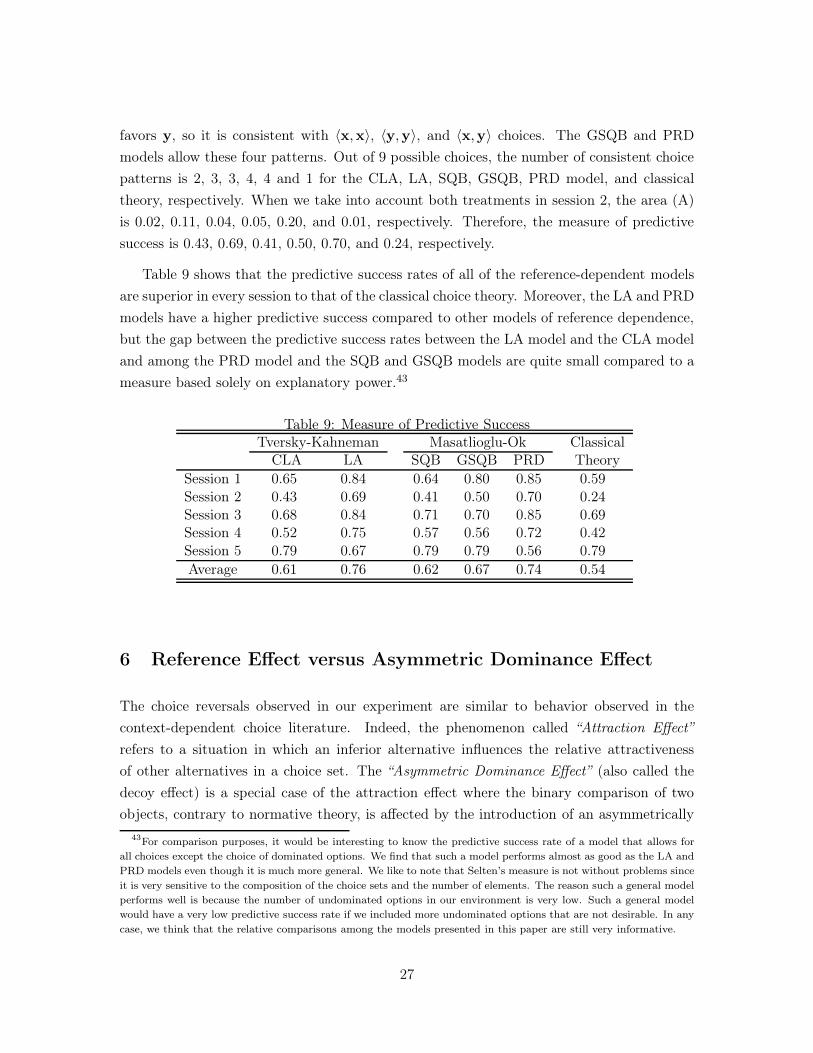
Table 9 shows that the predictive success rates of all of the reference-dependent models

are superior in every session to that of the classical choice theory. Moreover, the LA and PRD

models have a higher predictive success compared to other models of reference dependence,

but the gap between the predictive success rates between the LA model and the CLA model

and among the PRD model and the SQB and GSQB models are quite small compared to a

measure based solely on explanatory power.43

Table 9: Measure of Predictive SuccessTversky-Kahneman Masatlioglu-Ok Classical

CLA LA SQB GSQB PRD Theory

Session 1 0.65 0.84 0.64 0.80 0.85 0.59Session 2 0.43 0.69 0.41 0.50 0.70 0.24Session 3 0.68 0.84 0.71 0.70 0.85 0.69Session 4 0.52 0.75 0.57 0.56 0.72 0.42Session 5 0.79 0.67 0.79 0.79 0.56 0.79

Average 0.61 0.76 0.62 0.67 0.74 0.54

6 Reference Effect versus Asymmetric Dominance Effect

The choice reversals observed in our experiment are similar to behavior observed in the

context-dependent choice literature. Indeed, the phenomenon called “Attraction Effect”

refers to a situation in which an inferior alternative influences the relative attractiveness

of other alternatives in a choice set. The “Asymmetric Dominance Effect” (also called the

decoy effect) is a special case of the attraction effect where the binary comparison of two

objects, contrary to normative theory, is affected by the introduction of an asymmetrically

43For comparison purposes, it would be interesting to know the predictive success rate of a model that allows for

all choices except the choice of dominated options. We find that such a model performs almost as good as the LA and

PRD models even though it is much more general. We like to note that Selten’s measure is not without problems since

it is very sensitive to the composition of the choice sets and the number of elements. The reason such a general model

performs well is because the number of undominated options in our environment is very low. Such a general model

would have a very low predictive success rate if we included more undominated options that are not desirable. In any

case, we think that the relative comparisons among the models presented in this paper are still very informative.

27

dominated alternative to an existing choice set.

One could argue that the experimental evidence reported in the reference-dependent lit-

erature, including our paper, has nothing to do with ownership, but is rather an observation

of the decoy effect. A much more convincing argument would be that, in both situations,

the third alternative is used as a reference point and whether it is named as an endowment

or not does not make any difference. It is crucial to know whether the influence of the

status quo and the decoy option in people’s choice behavior are exactly the same or not.

Our experiment has additional choice problems that study the difference between decoy and

endowment.44 We study two related research questions. i) Does a status quo option affect

the relative rankings of alternatives more than a decoy option? ii) Does endowment matter

when it is not presented as the decoy option?

In order to answer our first question, we ask three choice problems for a given x-y pair.

We first elicit each subject’s preferences over x and y. Hence the first choice problem is

({x,y}, ⋄) where ⋄ denotes that there is no status quo. If the option x (y) is preferred, then

in another question the third option, z, which is dominated by the other alternative y (x),

is introduced and subjects are asked to choose from ({x,y, z}, ⋄), which is the second choice

problem. In the third choice problem, option z is given as the endowment while the set of

available options is the same set, i.e., ({x,y, z}, z). If being endowed with an option has

any bite, we expect to see different outcomes for the second and third decision problems.

Particularly, y (x) is chosen more when z is the endowment.

The percentage of switches when a status quo is introduced is 29%, compared to the

18% when a decoy option is introduced.45 Out of 79 subjects, 52 never change their initial

choice. 13 subjects change their choice when the third option is introduced as a status quo

option but not when it is introduced as a decoy option. Only 4 subjects change their choice

when the third option is introduced as a decoy option but not when it is introduced as an

endowment. 10 subjects show choice reversal at both times. Logistic regression analysis

shows that the odds of a choice reversal is 1.91 times greater when the reference point is

introduced as an endowment than when it is introduced as a decoy option (p = 0.028).

The above analysis shows that while the decoy effect is present in our data, this effect

is augmented when the dominated option is introduced as a reference point. However, it

is still not clear whether this establishes the importance of ownership. An alternative view

could be that when the decoy option is called the endowment, subjects’ attention is diverted

to the decoy option, which makes the decoy option more salient. Hence, the decoy effect

becomes stronger.

44We also control for the order effect in this part of the design by changing the order of the questions across sessions.45In this analysis we eliminated 1 observation in which dominated option was selected.

28

To test this alternative view, we consider a pair of decision problems: ({x,y, z}, ⋄) and

({x,y, z},y), where z is asymmetrically dominated by y.46 In the second choice problem,

the endowment and the decoy option are two separate bundles. Hence, the decoy option is

not highlighted by the presence of the endowment. If being endowed with an option has no

influence on choice behavior, i.e., the decoy option is the reference point, then the choice

behavior should be the same in these two choice problems.

Out of 97 subjects, 83 did not change their decisions when they were endowed with y.47

12 subjects changed their decisions in favor of y, and only 2 subjects changed their decisions

in favor of x. When a status quo is introduced, participants are more likely to choose the

alternative y (p = 0.006, robust odds ratio=1.54).

Note that the status quo introduced here is very weak since subjects do not actually

own them. However, even in the presence of a weak entitlement we see the effect of a status

quo. In a setting where individuals actually own the status quo option, we expect to see

even more striking effects on choices.

7 Literature Review and Discussion

The closest papers to ours are Bateman et al. [1997] and Herne [1998]—they provide com-

prehensive tests of the model of Tversky and Kahneman [1991]. Bateman et al. [1997] elicits

individual valuations of private goods using a laboratory experiment with eight different

measures. They find that implications of the general loss aversion model on valuations are

supported by their data. In particular, Bateman et al. find a divergence between these mea-

sures of valuation consistent with what is predicted by the model of Tversky and Kahneman

[1991]. Herne [1998], which considers a choice environment with asymmetrically domi-

nated reference points, provides direct tests of the loss aversion and diminishing sensitivity

hypotheses. The results of Herne’s experiments are consistent with the general reference-

dependent model of Tversky and Kahneman [1991]. In particular, Herne finds support for

loss aversion and diminishing sensitivity phenomena under asymmetrically dominated ref-

erence points using a between-subjects design (and, hence, individual factors cannot be

controlled for).

To our knowledge, our paper is the first to study different models of reference dependence

46Note that we do not elicit the preferences between the x-y pair in an effort not to repeat the same bundles too

much, and hence the decoy/endowment option is exogenously placed. Therefore, we expect to observe fewer choice

reversals, and this does not affect the decoy or endowment option differently. The decoy option is placed near the

higher money bundle once and higher chocolate bundle at another choice problem to control for any asymmetries due

to preferences across money and chocolate (see instructions to the experiment).47In this analysis we eliminated two observations in which dominated option was selected.

29

in a unified manner and disentangle critical behavioral properties that are satisfied by each

model. Our paper analyzes the reference effect by distinguishing the possible effects of

both asymmetrically and symmetrically dominated reference points. In addition, due to our

within-subjects design, we are able to contrast the models of reference dependence according

to their predictive success rates (which accounts for both predictive and explanatory powers

of the models).

As we have already mentioned, our paper is also related to the asymmetric dominance

effect in the literature on context dependence. Huber et al. [1982] is the first paper to

document that the addition of an asymmetrically dominated alternative (decoy) increases

the proportion of choices in favor of the target (dominating alternative). Ratneshwar et al.

[1987] shows that meaningfulness and familiarity with the product category moderates the

attraction effect compared to the Huber et al. [1982] study. However, the effect does not

disappear.

Simonson [1989], Simonson and Tversky [1992], Tversky and Simonson [1993], Ariely

and Wallsten [1995], and Wedell and Pettibone [1996] provide additional evidence and the-

oretical explanations for the asymmetric dominance effect, such as increasing justifiability

and tradeoff contrasts.48 Kivetz et al. [2004a,b] separate out four different groups of models

that explain context effects in general and test them. Three of these models can explain

asymmetric dominance effects and share a common feature with the models of Tversky and

Kahneman [1991].49 That is, the decision makers compare each alternative with a single

reference point. While in this paper the reference point is simply assumed to be the default

option, the models of Kivetz et al. [2004a] assume that the reference point is determined by

an exogenously given procedure. Depending on the model, the reference point is either the

midpoint or the minimum of the range of objective attribute levels in the choice set. If the

choice set changes, so does the reference point, and hence the reference point is context de-

pendent. One important fact is that the reference points in these models do not necessarily

belong to the choice set.

In our experiments changing the default option affects the composition of the choice set.

It would be interesting to know whether these models are also capable of accommodating

our data. To utilize these models, one should implicitly assume that the decision makers

are not affected by the default option directly. Nevertheless, the default option indirectly

affects the final choices by altering the composition of choice. Given our experimental

48In addition, Wedell and Pettibone [1996] studies context dependence under symmetrically dominated decoy

options. They do not observe an effect of adding a symmetrically dominated decoy option on choice. However, they

do not study the effect of shifting the decoy option in this region like we do in our study. In any case, it is encouraging

to find similar results.49These are the contextual concavity model, the normalized contextual concavity model, and the loss aversion

model. Please see Kivetz et al. [2004a,b] for the details of these models.

30

setup, two of these models, the contextual concavity model and the (context-dependent)

loss aversion model, were successful in accommodating and predicting the choice behavior.

Since these models are mostly making predictions similar to the LA model of Tversky and

Kahneman [1991], our findings for the LA model also applies to these models. The third

model, the normalized contextual concavity model, is too general to make any prediction

in our experimental set-up. The main advantage of these models is that they can account

for the changes in context even when the default option is fixed across different choice

sets. However, these models are short of explaining our findings in Section 6—the choices

are different under the same context. This is not surprising because these models do not

distinguish the default option from other alternatives in the choice set, i.e., reference points

in these models do not change when an option is presented as a default or not. Hence these

models cannot capture the differences in choices between the decision problems presented

in Section 6.50

This paper provides a bridge between literatures on context dependence and reference

dependence. We find that even the presence of a weak entitlement (decoy option is referred

to as a default option) has an effect on choice beyond the effect of adding a decoy option

to the choice set. It might be argued that this is because a default option reinforces the

context effect. While this might be some part of the explanation, we show that there is

also an additional and independent effect of entitlement (i.e., entitlement affect choices even

when it is not presented as the decoy option). Future research should provide theories that

could accommodate both the effect of a default option and context dependence.

8 Conclusion

This paper is an additional step towards understanding reference-dependent choice behav-

iors. Our contribution to the literature is two-fold. First, we contrast reference-dependent

models by providing which behavioral properties that they satisfy. Then, we design an ex-

periment to test these properties and to understand reference effect. In our experiment,

we find strong evidence for the existence of the reference effect: reference points alter one’s

choices even when agents do not choose the reference point itself. In particular, we find

that the reference effect exists for asymmetrically dominated reference points, but we do not

observe any evidence of the reference effect for symmetrically dominated reference points.

With respect to behavioral properties we find support for ISD and DSA. In addition, we

document the predictive success rates of different models. We believe that these results not

only help us compare the existing reference-dependent models but also provide guidance for

50Unfortunately, we could not see an obvious way to modify these models to accommodate findings in Section 6.

31

future modeling choices.

We now provide a general assessment of the existing models. All the models under

consideration have advantages over others. Some enjoy high predictive power; while others

have high explanatory power. In our view, both the LA model and the PRD model are too

general to be useful in applications. For example, the LA model does not even satisfy the

fundamental and most-illustrated property of SQBP (see Sagi [2006], Masatlioglu and Ok

[2010]). Hence, the LA model allows for the prediction that is opposite of what Tversky and

Kahneman [1991] initially intended to explain.51 While we do not test the well-documented

SQBP, one can imagine that had we included that in our design, the predictive success rate

of the LA model would diminish dramatically. On the other hand, the PRD model satisfies

SQBP but fails to make powerful predictions. In sum, even though these models are capable

of accommodating most of our data, they lack prediction power.

The CLA model is the most restricted model and requires no reference effect for asym-

metrically dominated reference points. We have seen that this prediction is not consistent

with our data. Hence, it cannot be a canonical model if one wants to investigate the im-

plications of asymmetrically dominated reference points. Similarly, the SQB model is also

too restrictive. Unlike the CLA model, the model predicts that asymmetrically dominated

reference points influence behavior, but the prediction of this model is not supported in our

data for this particular case.

Finally, the GSQB model seems to be the winner of all, since it has the right combina-

tion of high predictive and explanatory power. The model predicts that there is no reference

effect for symmetrically dominated reference points and allows for reference effect for asym-

metrically dominated reference points at the same time.52 In addition to that, it satisfies

the key property of status quo bias. Moreover, the GSQB model is consistent with both the

presence and absence of a gap between willingness-to-accept and willingness-to-pay.53

Our paper has implications regarding the economic policies that impose default options

such as retirement plans. It has been shown that the automatic enrollment tends to anchor

employee asset allocations on the automatic enrollment default asset allocation.54 More

strikingly, the default allocation affects the asset allocations of those workers who abandon

51In addition to that, there are other implications of the LA model, which contradict the empirical facts: (i) it

permits non-convex indifference curves (Munro and Sugden [2003]), (ii) it is impossible to make welfare comparisons

under this model (Mandler [2004]), and (iii) it necessitates a discrepancy between willingness-to-accept (WTA) and

willingness-to-pay (WTP) (Plott and Zeiler [2005] and List [2003, 2004]).52While we find the GSQB model to be the most reasonable model among the current models, there is still room

for improvement, since the GSQB model does not satisfy the DSA property.53For a detailed explanation, see Masatlioglu and Ok [2010].54Beshears et al. [2006] shows that while 86% of employees who were subject to automatic enrollment have some of

their assets allocated to the default fund, this number is only 10% for employees who were not subject to automatic

enrollment (they were hired and initiated savings plan participation before automatic enrollment).

32

their default plan. Our findings add to this literature that default options may have a strong

impact on choices, even when they are not chosen. More importantly, we demonstrate the

impact of different default options on choices. In particular, asymmetrically dominated

reference points would have an impact on decisions; however, we do not expect symmetrically

dominated asset allocations to influence employee decisions once the default allocation is

deserted. This enables policy makers to derive important policy implications regarding the

interaction of a default allocation and employee savings. Consequently, employers may be

able to help their employees achieve desired retirement goals.

Appendix

A. Theoretical Predictions and Proofs of Proposition 1 and 2

We now illustrate the predictions of each model for five different reference shifts: ⋄ → x,

l → l′, l′ → l′′, s → s′, and a → a′. This will also prove both Proposition 1 and 2.

The CLA model: Since each gi is linear and satisfies loss aversion, w.l.o.g., we

assume gi(a) = a when a ≥ 0 and gi(a) = λa when a < 0, for i = 1, 2 and where λ > 1. We

also normalize u1(0) = u2(0) = 0.

(⋄ → x): x ∈ c({x,y}, ⋄) implies that 0 ≤ U(0,0)(x)−U(0,0)(y) = u1(x1)−u1(y1)+u2(x2)−u2(y2). Hence, x provides more than y for at least one of the dimensions, say dimension

1. Then we have Ux(y) = λ(u1(y1)− u1(x1)) + u2(y2)− u2(x2). Since λ > 1, we have

Ux(y) < u1(y1) − u1(x1) + u2(y2) − u2(x2). By assumption, the right-hand side is

less than 0. Therefore, Ux(y) < 0 = Ux(x), x = c({x,y},x). As a result, SQBP is

satisfied.

(l → l′): The CLA model implies that Ul(x)−Ul′(x) = u1(l′1)−u1(l1) and Ul(y)−Ul′(y) =

λ(u1(l′1) − u1(l1)). Since λ > 1, we have Ul(y) − Ul′(y) > Ul(x) − Ul′(x). Arrange

the terms to get Ul′(x) − Ul′(y) > Ul(x) − Ul(y). Since x ∈ c({x,y, l}, l), we have

Ul(x)−Ul(y) > 0, so Ul′(x)−Ul′(y) ≥ 0. Therefore, x = c({x,y, l′}, l′), which implies

WLAP is a necessary condition.

(l′ → l′′): Since the illustration is exactly the same as above, we skip it. In sum, SLAP is

also a necessary condition.

(s → s′): We have Us(x) − Us′(x) = u1(s′1) − u1(s1) = Us(y) − Us′(y). Therefore, there is

no change in the relative ranking of x and y as we move the reference point. Hence,

the model predicts no change, which means ISD holds. Moreover, DSS is violated.

33

(a → a′): Since the illustration of the s → s′ shift also applies here, we skip the proof. In

sum, IAD is also a necessary condition. �

The LA model: Again normalize u1(0) = u2(0) = 0.

(⋄ → x): Since the CLA model is a special case, the LA model can accommodate status

quo bias. On the other hand, Masatlioglu and Ok [2010] provides an example where

the LA model predicts status quo aversion. Hence, this model makes no particular

prediction for this type of shifts, so indecisive.

(l → l′): We demonstrate the theoretical predictions for the case of switching the reference

point from l to l′. In the LA model, the utility gains of x and y from the l − l′

shift are Ul′(x) − Ul(x) = g1(u1(x1) − u1(l′1)) − g1(u1(x1) − u1(l1)) and Ul′(y) −

Ul(y) = g1(u1(y1)−u1(l′1)), respectively. All utility differences are in terms of the first

dimension since l2 = l′2. Note that u1(x1)− u1(l1) = u1(x1)− u1(l′1) +u1(l

′1)− u1(y1)

since y1 = l1. The concavity of gi|R+

55 implies that

g1(u1(x1)− u1(l′1))− g1(u1(x1)− u1(l1)) ≥ −g1(u1(l

′1)− u1(y1))

> g1(u1(y1)− u1(l′1))

since gi(a) < −gi(−a) for a > 0. Hence, we have Ul′(x) − Ul(x) > Ul′(y) − Ul(y).

Rearranging this inequality gives us Ul′(x)−Ul′(y) > Ul(x)−Ul(y) ≥ 0, which means

that switching from l to l′ favors x. This implies WLAP is a necessary condition.

(l′ → l′′): Since the CLA model is a special case of this model, the LA model also allows

that this shift favors x. On the other hand, it is easy to create examples such that

x1 = l′′1 > l′1 > y1 and y2 > x2 > l′2 = l′′2 and while x is chosen under l′, y is

chosen under l′′. For example, assume that gi(a) = a0.5 when a ≥ 0 and gi(a) =

−2(−a)0.5 when a < 0 for i = 1, 2. In addition, assume that the utility differences in

dimension 1 are u1(l′1)− u1(y1) = 16 and u1(x1)− u1(l

′1) = 9 and in dimension 2 are

u2(y2)− u2(l′2) = 144 and u2(x2)− u2(l

′2) = 1. Then we have Ul′(x) = 90.5 + 10.5 = 4

and Ul′(y) = −2 ∗ 160.5 + 1440.5 = 4. Hence, x ∈ c({x,y, l′}, l′). On the other hand,

Ul′′(x) = 00.5+10.5 = 1 and Ul′′(y) = −2∗250.5+1440.5 = 2. Hence x /∈ c({x,y, l′}, l′).In sum, the model makes no prediction, and SLAP is not a necessary condition.

(a → a′): The utility losses of x and y from switching are Ua(x) − Ua′(x) = g1(u1(x1) −u1(a1))− g1(u1(x1)− u1(a

′1)) and Ua(y)−Ua′(y) = g1(u1(y1)− u1(a1))− g1(u1(y1)−

u1(a′1)), respectively. All utility differences are in terms of the first dimension since

55If f is an increasing concave function and f(0) = 0, then we have f(x) + f(y) ≥ f(x+ y) for all x, y ≥ 0.

34

a2 = a′2 and positive. Let β = u1(a′1)− u1(a1). Then we have

Ua(x)− Ua′(x) = g1(u1(x1)− u1(a′1) + β)− g1(u1(x1)− u1(a

′1))

< g1(u1(y1)− u1(a′1) + β)− g1(u1(y1)− u1(a

′1))

< Ua(y) − Ua′(y)

The second line in the above equation is derived by utilizing the concavity of gi|R+

and u1(x1) > u1(y1).56 This means that switching from a to a′ increases x’s relative

ranking with respect to y. In addition, if x is chosen at a (Ua(x) − Ua(y) ≥ 0), then

x will be uniquely chosen at a′ (Ua′(x) − Ua′(y) > Ua(x) − Ua(y) ≥ 0). Therefore,

DSA is a necessary condition for the model.

(s → s′): This shift also increases x’s relative ranking with respect to y. For the proof,

please see the demonstration of a → a′ shift. Thus, DSS is also a necessary condition

for the model. �

The SQB model:

(⋄ → x): The model is built on a property that is even stronger than SQBP: x ∈ c(S,y)

implies x = c(S,x) (Masatlioglu and Ok [2005]). Hence, it also satisfies SQBP.

(l → l′): By definition, x is in both Q(l) and Q(l′), and Q(l′) ⊂ Q(l). If x ∈ c({x,y, l}, l),then x is best in Q(l)∩{x,y, l}. Since Q(l′) ⊂ Q(l), x must be best in Q(l′)∩{x,y, l′}.Therefore, x ∈ c({x,y, l′}, l′), which implies WLAP is a necessary condition.

(l′ → l′′): Since the illustration is exactly the same as above, we skip the proof. In sum,

SLAP is also a necessary condition.

(s → s′): ISD is one of the axioms of the model. Hence, the model predicts no change.

Thus, DSS is not a necessary condition for this model.

(a → a′): If y ∈ c({x,y,a},a), then y is best in Q(a) ∩ {x,y,a}. Since y ∈ Q(a′) ⊂ Q(a),

y must be best in Q(a′) ∩ {x,y,a′}. Therefore, y ∈ c({x,y,a′},a′): an a → a′ shift

favors y. As a result, DSA is not implied by the SQB model. �

The GSQB model:

(⋄ → x): The model is built on SQBP (Masatlioglu and Ok [2010]).

56If f is a strictly increasing concave function, then we have f(a + β)− f(a) < f(b+ β)− f(b) whenever a > b.

35

(l → l′): Since x dominates l′ both dimensions, x must be in Q(l′). Similarly, y is in Q(l).

Given that y is in the constraint set, if x ∈ c({x,y, l}, l), then U(x) must yield a

utility as high as U(y). Hence, x must be best in Q(l′) ∩ {x,y, l′} since x ∈ Q(l′).

Therefore, x ∈ c({x,y, l′}, l′). Switching from l to l′ favors x, which implies WLAP is

a necessary condition.

(l′ → l′′): We show that the model does not make any particular prediction for this shift.

In other words, the model is indecisive. The argument for the SQB model does not

hold since we no longer know whether y is in Q(l′) or not. Hence, it is possible that

x is chosen while y is not in Q(l′) and provides higher utility than x. When the

reference point shifts to l′′, y might be included in Q(l′′), which makes y the best in

Q(l′′) ∩ {x,y, l′′}. Hence, it is possible that y ∈ c({x,y, l′′}, l′′). On the other hand,

since the SQB model is a special case of this model, the model can generate cases

where x is favored. Therefore, the model does not make any prediction. In other

words, SLAP is not a necessary condition for this model.

(s → s′): ISD is one of the axioms of the model. Hence, the model predicts no change.

Thus, DSS is not a necessary condition for this model.

(a → a′): The model is indecisive. Since the SQB model favors y, the model can generate

cases where y is favored. We now show the other possibility. Consider an a → a′ shift

where y is chosen while x is not in Q(a) and provides higher utility than x. When

the reference point shifts to a′, x might be included in Q(a′), which makes x is best

in Q(a′) ∩ {x,y,a′}. Hence, it is possible that x ∈ c({x,y,a′},a′). Both cases are

consistent with the model. Thus, DSA is not a necessary condition for this model. �

The PRD model:

(⋄ → x): The model is built on SQBP (Masatlioglu and Ok [2007]).

(l → l′): The model is indecisive. Since the SQB model favors x, this model also favors x

for some cases. We now show that there are other cases where the model favors y.

Consider a case where U(y) > U(x), x is in Q1(l) \ Q1(l′) and y is in Q2(l′) \ Q1(l).

Since {x,y} ∩ Q1(l) = {x}, x is selected when l is the reference point (Q1 will be

utilized). When l′ is the reference point, y is selected since U(y) > U(x). Therefore

the model favors y for this case. Switching from l to l′ has no implication, which

implies WLAP is not a necessary condition.

(l′ → l′′): Similar to above, and hence SLAP is not a necessary condition.

36

(s → s′): The model is indecisive. Consider a case where U(y) > U(x), x is in Q1(s)\Q1(s′)

and y is in Q2(s′)\Q1(s). Then x is selected when s is the reference point (Q1 will be

utilized), and y is selected when s′ is the reference point. Therefore the model favors

y for this case. Since everything is symmetric, if we switch the roles of x and y, we

get an opposite prediction. Switching from s to s′ has no implication (ISD and GSS

do not hold).

(a → a′): The model is indecisive except at the boundary (where y2 = a2 = a′2).

First, consider the cases without this boundary. Since the SQB model favors y, the

model can generate cases where y is favored. We now illustrate the other possibility.

Consider an a → a′ shift. Assume that (i) x provides more utility than y (U(x) >

U(y)), and (ii) x is not in Q1(a), but y is in. Hence y is chosen when the reference

point is a. Further assume (i) when the reference point shifts to a′, y is excluded in

Q1(a′), and (ii) both x,y are in Q2(a′). Then we have x ∈ c({x,y,a′},a′), so x is

favored in this case. Switching from a to a′ has no implication (IAD and DSA do not

hold).

For the boundary case, these type of shifts favor y as does the SQB model. Since

Q1 includes only strictly dominating alternatives, neither x nor y belongs to Q1(a) or

Q1(a′). Hence, only Q2 has a bite in this case. Given that Q2 satisfies (i)-(iii), the

PRD model behaves same as the SQB model for these type of shifts. �

B. A Screenshot

Figure 5: A screenshot from the experiment

37

References

D. Ariely and T. S. Wallsten. Seeking subjective dominance in multidimensional space: Anexplanation of the asymmetric dominance effect. Organizational Behavior and HumanDecision Processes, 63(3):223 – 232, 1995.

D. Ariely, G. Loewenstein, and D. Prelec. Coherent arbitrariness: Stable demand curveswithout stable preferences. The Quarterly Journal of Economics, 118(1):73–105, 2003.

D. Bateman, I. Kahneman, A. Munro, B. Rhodes, C. Starmer, and R. Sugden. Testing com-peting models of loss aversion: an adversarial collaboration. Journal of Public Economics,89:1561–1580, 2005.

I. Bateman, A. Munro, B. Rhodes, C. Starmer, and R. Sugden. A test of the theory ofreference-dependent preferences. Quarterly Journal of Economics, 112:479–505, 1997.

J. Beshears, J. J. Choi, D. I. Laibson, and B. C. Madrian. The importance of default optionsfor retirement savings outcomes: Evidence from the united states. NBER Working PaperNo. W12009, 2006.

M. Chaves and J. D. Montgomery. Rationality and the framing of religious choices. Journalfor the Scientific Study of Religion, 35(2):128–144, 1996.

J. J. Choi, D. Laibson, B. C. Madrian, and A. Metrick. For better or for worse: Default effectsand 401(k) savings behavior. Technical Report 256, Northwestern University/Universityof Chicago Joint Center for Poverty Research, 2002.

M. Dean. Status quo bias in large and small choice sets. mimeo, 2008.

K. Herne. Testing the refence-dependent model: An experiment on asymmetrically domi-nated reference points. Journal of Behavioral Decision-Making, 11:181–192, 1998.

J. K. Horowitz and K. E. McConnell. A review of wta/wtp studies. Journal of EnvironmentalEconomics and Management, 44(3):426–447, 2002.

N. Houy. Choice functions with states of mind. Theory and Decision, 53:1–26, 2007.

J. Huber, J. Payne, and C. Puto. Adding asymmetrically dominated alternatives: Violationsof regularity and the similarity hypothesis. Journal of Consumer Research, 9:90–98, 1982.

E. Johnson and D. Goldstein. Do defaults save lives? Science, 302:1338– 1339, 2003.

E. Johnson, J. J. Hershey, J. Meszaros, and H. Kunreuther. Framing, probability distortions,and insurance decisions. Journal of Risk and Uncertainty, 7:35–51, 1993.

E. S. G. Johnson and A. Hermann. Exploring the nature of loss aversion. mimeo, 2006.

M. U. Kalwani, C. K. Yim, H. J. Rinne, and Y. Sugita. A price expectations model ofcustomer brand choice. Journal of Marketing Research, 27(3):251–262, 1990.

38

G. Kalyanaram and J. D. C. Little. An empirical analysis of latitude of price acceptance inconsumer package goods. The Journal of Consumer Research, 21(3):408–418, 1994.

K. Kawai. Status quo bias and incomplete preferences. mimeo, Kyoto University, 2008.

R. Kivetz, O. Netzer, and V. Srinivasan. Extending compromise effect models to complexbuying situations and other context effects. Journal of Marketing Research, 41(3):262–268,2004a.

R. Kivetz, O. Netzer, and V. Srinivasan. Alternative models for capturing the compromiseeffect. Journal of Marketing Research, 41(3):237–257, 2004b.

L. Knetsch. The endowment effect and evidence of nonreversible indifference curves. Amer-ican Economic Review, 79:1277–1284, 1989.

B. Köszegi and M. Rabin. A model of reference-dependent preferences. Quarterly Journalof Economics, 121(4):1133–1165, 2006.

J. List. Does market experience eliminate market anomalies? Quarterly Journal of Eco-nomics, 118:41–71, 2003.

J. List. Neoclassical theory versus prospect theory: Evidence from the market place. Econo-metrica, 72:615–625, 2004.

G. Loewenstein and D. Adler. A bias in the prediction of tastes. The Economic Journal,105(431):929–937, 1995.

B. C. Madrian and D. F. Shea. The power of suggestion: Inertia in 401(k) participation andsavings behavior. The Quarterly Journal of Economics, 116(4):1149–1187, 2001.

M. Mandler. Status quo maintenance reconsidered: changing or incomplete preferences?Economic Journal, 114:518–535, 2004.

Y. Masatlioglu and E. A. Ok. Rational choice with status quo bias. Journal of EconomicTheory, 121:1–29, 2005.

Y. Masatlioglu and E. A. Ok. Reference-dependent procedural decision making. mimeo,2007.

Y. Masatlioglu and E. A. Ok. A canonical model of choice with initial endowments. mimeo,2010.

G. E. Mayhew and R. S. Winer. An empirical analysis of internal and external referenceprices using scanner data. The Journal of Consumer Research, 19(1):62–70, 1992.

A. Munro and R. Sugden. On the theory of reference-dependent preferences. Journal ofEconomic Behavior Organization, 50(4):407–428, 2003.

C. W. Park, S. Y. Jun, and D. J. MacInnis. Choosing what i want versus rejecting what i donot want: An application of decision framing to product option choice decisions. Journalof Marketing Research, 37(2):187–202, 2000.

39

C. R. Plott and K. Zeiler. The willingness to pay-willingness to accept gap, the "endowmenteffect," subject misconceptions, and experimental procedures for eliciting valuations. TheAmerican Economic Review, 95(3):530–545, 2005.

C. R. Plott and K. Zeiler. Exchange asymmetries incorrectly interpreted as evidence ofendowment effect theory and prospect theory? American Economic Review, 97(4):1449–1466, 2007.

D. S. Putler. Incorporating reference price effects into a theory of consumer choice. MarketingScience, 11(3):287–309, 1992.

S. Ratneshwar, A. D. Shocker, and D. W. Stewart. Toward understanding the attractioneffect: The implications of product stimulus meaningfulness and familiarity. Journal ofConsumer Research, 13(4):pp. 520–533, 1987.

J. S. Sagi. Anchored preference relations. Journal of Economic Theory, 127(1):283–295,2006.

R. Selten. Properties of a measure of predictive success. Mathematical Social Sciences, 21(2):153 – 167, 1991.

R. Selten and S. Krischker. Comparison of two theories for characteristic function experi-ments. Springer, Berlin and Heidelberg, 1983.

I. Simonson. Choice based on reasons: The case of attraction and compromise effects.Journal of Consumer Research, 16:158–174, 1989.

I. Simonson and A. Tversky. Choice in context: Tradeoff contrast and extremeness aversion.Journal of Marketing Research, 29:281–295, 1992.

R. Sugden. Reference-dependent subjective expected utility. Journal of Economic Theory,111:172–191, 2003.

I. G. Tapki. Revealed incomplete preferences under status-quo bias. Mathematical SocialSciences, 53(3):274–283, 2007.

A. Tversky and D. Kahneman. Loss aversion in riskless choice: A reference-dependent model.The Quarterly Journal of Economics, 106(4):1039–1061, 1991.

A. Tversky and I. Simonson. Context-dependent preferences. Management Science, 39:1179–1189, 1993.

P. Wakker and A. Tversky. An axiomatization of cumulative prospect theory. Journal ofRisk and Uncertainty, 17(7):147–176, 1993.

D. H. Wedell and J. C. Pettibone. Using judgments to understand decoy effects in choice.Organizational Behavior and Human Decision Processes, 67(3):326 – 344, 1996.

40