UNDERSTANDING THE ROLE OF SHAFT STIFFNESS IN THE GOLF

SWING

A Thesis Submitted to the College of

Graduate Studies and Research in Partial

Fulfillment of the Requirements for the

Degree of Doctor of Philosophy in the

College of Kinesiology

University of Saskatchewan

Saskatoon, Saskatchewan

By

Sasho J. MacKenzie

© Copyright Sasho J. MacKenzie, December 2005. All rights reserved.

PERMISSION TO USE

In presenting this thesis in partial fulfillment of the requirements for a

Postgraduate degree from the University of Saskatchewan, I agree that the Libraries of

the University may make it freely available for inspection. I further agree that

permission for copying of this thesis in any manner, in whole or in part, for scholarly

purposes may be granted by the professor or professors who supervised my thesis work

or, in their absence, by the Head of the Department or the Dean of the College in which

this thesis work was done. It is understood that any copying or publication or use of this

thesis or parts thereof for financial gain shall not be allowed without my written

permission. It is also understood that due recognition shall be given to me and the

University of Saskatchewan in any scholarly use which may be made of any material in

my thesis.

Requests for permission to copy or to make any other use of material in this

thesis in whole or in part should be addressed to:

The Dean

College of Kinesiology

University of Saskatchewan

87 Campus Drive

Saskatoon, Saskatchewan, Canada, S7N 5B2

i

ACKNOWLEDGEMENT

I would like to thank my supervisor, Dr. Eric Sprigings and my committee

members, Dr. Gordon Binsted, Dr. Denise Stilling, and Dr. Glen Watson for their

support and advice throughout the preparation and completion of this thesis. I would

also like to thank Dr. Mont Hubbard for acting as the external examiner.

I would like to thank Dr. Graham Caldwell and Dr. Joseph Hamill for providing

me with the opportunity to further my understanding of biomechanics in their research

laboratory. Your welcome was warm, expertise invaluable, and guidance appreciated.

I would like to acknowledge the Natural Sciences and Engineering Research

Council of Canada for providing funding support during the completion of this thesis.

ii

ABSTRACT

The purpose of this thesis was to determine how shaft stiffness affects clubhead

speed and how it alters clubhead orientation at impact. For the first time, a 3D, six-

segment forward dynamics model of a golfer and club was developed and optimized to

answer these questions. A range of shaft stiffness levels from flexible to stiff were

evaluated at three levels of swing speed (38, 45 and 53 m/s). At any level of swing

speed, the difference in clubhead speed did not exceed 0.1 m/s across levels of shaft

stiffness. Therefore, it was concluded that customizing the stiffness of a golf club shaft

to perfectly suit a particular swing will not increase clubhead speed sufficiently to have

any meaningful effect on performance. The magnitude of lead deflection at impact

increased as shaft stiffness decreased. The magnitude of lead deflection at impact also

increased as swing speed increased. For an optimized swing that generated a clubhead

speed of 45 m/s, with a shaft of regular stiffness, lead deflection of the shaft at impact

was 6.25 cm. The same simulation resulted in a toe-down shaft deflection of 2.27 cm at

impact. Using the model, it was estimated that for each centimeter of lead deflection of

the shaft, dynamic loft increased by approximately 0.8°. Toe-down shaft deflection had

relatively no influence on dynamic loft. For every centimeter increase in lead deflection

of the shaft, dynamic closing of the clubface increased by approximately 0.7°. For

every centimeter increase in toe-down shaft deflection, dynamic closing of the clubface

decreased by approximately 0.5°. The results from this thesis indicate that

improvements in driving distance brought about by altering shaft stiffness are the result

of altered clubhead orientation at impact and not increased clubhead speed.

iii

TABLE OF CONTENTS

PERMISSION TO USE i

ACKNOWLEDGEMENT ii

ABSTRACT iii

TABLE OF CONTENTS iv

LIST OF TABLES viii

LIST OF FIGURES ix

CHAPTER 1 INTRODUCTION TO THE STUDY 1

1.1 Introduction 2

1.2 Literature Review of Shaft Bending 4

1.2.1 Shaft Bending During the Swing 4

1.2.2 Utilization of Energy Stored in the Shaft 9

1.2.3 Variations in Force and Torque Patterns applied to the Club 14

1.2.4 Changes in Clubhead Orientation due to Shaft Deflection 16

1.2.5 Cause of Shaft Bending from a Newtonian Perspective 16

1.2.5.1 Tangential Force Component 17

1.2.5.2 Radial Force Component 18

1.2.6 Optimization of Shaft Behaviour 20

1.3 Statement of Problem and Hypotheses 22

1.3.1 The Problem 22

1.3.2 Research Hypotheses 22

1.4 Review of Optimized Forward Dynamic Simulations 23

iv

1.4.1 Develop the Physical Properties of each Segment 25

1.4.2 Provide the Model with the Ability to Generate Motion 28

1.4.3 Develop Equations that will Govern the Motion of the Model 32

1.4.4 Determine How the Equations will be Solved 40

1.4.5 Implement an Optimization Scheme 42

CHAPTER 2 METHODS 50

2.1 Mathematical Model 51

2.1.1 General Description of Golfer-Club Model 51

2.1.2 Method for Measuring Shaft Deflection 56

2.1.3 Determining Shaft Stiffness and Damping Parameters 57

2.1.4 Equations of Motion 61

2.1.5 Generalized Coordinates of the Golfer Model 61

2.2 Optimization of the Golfer-Club Model 63

2.2.1 Customizing the Golfer to Fit the Club 64

2.2.2 Customizing the Club to Fit the Golfer 66

2.3 Simulated Thought Experiments Using the Golfer-Club Model 67

2.3.1 Use of a Perfectly Rigid Shaft 67

2.3.2 Repositioning the Clubhead Center of Mass 68

2.3.3 Removal and Isolation of Radial Force 69

2.3.4 Effect of Shaft Deflection on Clubhead Orientation 71

2.4 Model Validation 72

2.4.1 External Validity 72

2.4.1.1 Live Golfer Testing 72

v

2.4.1.2 Error and Reliability of Live Golfer Testing 77

2.4.1.3 Swing Plane Comparison 78

2.4.2 Internal Validity 79

CHAPTER 3 RESULTS 80

3.1 Optimization of the Golfer-Club Model 81

3.1.1 Typical Swing Results 81

3.1.2 Customizing the Golfer to Fit the Club 84

3.1.3 Customizing the Club to Fit the Golfer 91

3.2 Simulated Thought Experiments Using the Golfer-Club Model 94

3.2.1 Use of a Perfectly Rigid Shaft 94

3.2.2 Repositioning the Clubhead Center of Mass 97

3.2.3 Removal and Isolation of Radial Force 101

3.2.4 Effect of Shaft Deflection on Clubhead Orientation 106

3.3 Model Validation 108

3.3.1 External Validity 108

3.3.1.1 Live Golfer Testing 108

3.3.1.2 Error and Reliability of Live Golfer Testing 114

3.3.1.3 Swing Plane Comparison 115

3.3.2 Internal Validity 117

CHAPTER 4 DISCUSSION 119

4.1 The Relationship Between Shaft Stiffness and Clubhead Speed 120

4.2 The Relationship Between Shaft Stiffness and Clubhead Orientation 124

4.3 The Mechanisms Behind Shaft Bending 126

vi

4.4 The Role of Radial Force 129

4.5 Limitations of the Model 130

4.6 Limitations of the Live Golfer Testing 134

4.7 Conclusions 135

4.8 Future Directions 137

REFERENCES 146

APPENDIX A Consent Form, Ethical Approval 154

APPENDIX B Inertial Properties of Simulated Club Segments 157

APPENDIX C Autolev© Code: 3DGOLFG.AL 172

APPENDIX D Matlab© Code: GOLF3D.M 184

APPENDIX E FORTRAN© Code: 3DGOLFG.FOR 188

vii

LIST OF TABLES

Table 1.4.1.1 Parameter values for two segment golfer model. 28

Table 2.1.1.1 Six-segment golfer-club model segment parameters. 55

Table 2.1.3.1 Stiffness coefficients for rotational springs of simulated drivers. 60

Table 3.1.2.1 Measures of shaft bending during the swing and at impact

for 9 optimized golfer-club models. 86

Table 3.2.1.1 Clubhead speeds attained with rigid shafts and the highest

clubhead speeds attained with any of the three flexible shafts

for each of the three golfer models. 94

Table 3.3.1.1.1 Lead deflections and clubhead speeds at impact as determined

from Perspective 1. Values are the average and standard

deviations from three swings. Lead is presented in centimetres,

and clubhead speed is given in meters per second. 111

Table 3.3.1.1.2 Toe-down deflections at impact as determined from

Perspective 2. Values are given in centimetres, and

are the average and standard deviations for three swings. 114

viii

LIST OF FIGURES

Figure 1.2.1.1 Shaft deflection in the lead and toe-down directions. 5

Figure 1.2.5.1.1 Demonstration of the effect of tangential force on

shaft bending. 18

Figure 1.2.5.1.2 Demonstration of the effect of radial force on

shaft bending. 20

Figure 1.4.3.1 Schematic of two-segment golfer model. 37

Figure 1.4.3.2 Free-body diagram of two-segment golfer model. 38

Figure 1.4.5.1 Search space for a single variable optimization problem. 44

Figure 2.1.1.1 Six segment 3D golfer-club model. 52

Figure 2.1.1.2 The torso segment and arm segment were constrained to

rotate in specific planes. 54

Figure 2.1.2.1 Calculation of lead/lag shaft deflection along the y axis of

the shaft. Identical methods were used for calculating toe-up/

toe-down deflection along the x axis of the shaft. 57

Figure 2.1.3.1 Experimental set-up for determining shaft stiffness. 59

Figure 2.1.5.1 Graphical depiction of the generalized coordinates used in

Autolev© for developing the 3D golfer model. Diagram A

is from a perspective looking along the negative TILT3>

axis. Diagram B is from a perspective looking along the

positive TILT1> axis. 62

ix

Figure 2.4.1.1.1 Set-up of live golfer testing from Perspective 1. 74

Figure 2.4.1.1.2 Set-up of live golfer testing from Perspective 2. 75

Figure 3.1.1.1 Output from the four muscle torque generators during the

optimized execution of Golfer-Medium with Club-Regular. 82

Figure 3.1.1.2 Generalized coordinates of the golfer model as a function

of time. Shoulder rotation is provided relative to the

angular position of the trunk and not in absolute terms as

described in section 2.1.5 and in Appendix C. 84

Figure 3.1.2.1 Dynamic loft at impact from the 9 optimized simulations

in which the timing of each golfer model’s swing was fit to

each of the clubs. 87

Figure 3.1.2.2 Dynamic close at impact from the 9 optimized simulations

in which the timing of each golfer model’s swing was fit to

each of the clubs. 88

Figure 3.1.2.3 Toe-up/toe-down and lead/lag deflections during the

optimized execution of Golfer-Medium with Club-Regular.

The shaded area represents the time during which the

clubhead was deflected in the lag direction. 89

Figure 3.1.2.4 Kick velocity during the optimized execution of Golfer-

Medium with Club-Regular. 90

Figure 3.1.3.1 Resulting clubhead speed and clubhead speed minus penalties

over a complete range of shaft stiffness for a single swing

pattern from Golfer-Medium. 92

x

Figure 3.1.3.2 Resulting clubhead speed and clubhead speed minus penalties

over a complete range of shaft stiffness for a single swing

pattern from Golfer-Slow. 93

Figure 3.1.3.3 Resulting clubhead speed and clubhead speed minus penalties

over a complete range of shaft stiffness for a single swing

pattern from Golfer-Fast. 93

Figure 3.2.1.1 Angular velocity of the most proximal club segment for the

optimized simulations of Golfer-Medium with Club-Stiff and

Golfer-Medium with Club-Rigid. 96

Figure 3.2.2.1 Toe-up/toe-down deflections for three different clubhead

center of mass positions. Golfer-Medium/Club-Regular

was used for all three conditions. Normal refers to a

standard driver that has the center of mass located in

the toe-up direction relative to the shaft insertion point.

In-line refers to having the center of mass collinear

with the shaft. Reversed refers to having the center

of mass in the toe-down direction relative to the shaft. 98

Figure 3.2.2.2 Lead/lag deflections for three different clubhead center of

mass positions. Golfer-Medium/Club-Regular was used for

all three conditions. Normal refers to a standard driver that

has the center of mass located in the lag direction relative to

the shaft insertion point. In-line refers to having the center

of mass collinear with the shaft. Reversed refers to having

xi

the center of mass in the lead direction relative to the shaft. 100

Figure 3.2.3.1 Comparison of shaft deflections between the simulated swing

of Golfer-Medium with Club-Regular and the same swing with

radial force removed. 102

Figure 3.2.3.2 Shaft deflection when radial force acted in isolation of all other

forces and torques supplied by Golfer-Medium to Club-Regular

during the optimized swing. 104

Figure 3.2.3.3 Radial force acting along the z axis of the most proximal

club segment during the optimized swing of Golfer-Medium

with Club-Regular. 105

Figure 3.2.4.1 Three-dimensional plot of dynamic loft as a function of both

lead and toe-down deflections. 106

Figure 3.2.4.2 Three-dimensional plot of dynamic close as a function of both

lead and toe-down deflections. 107

Figure 3.3.1.1.1 In-plane shaft deflection during the downswing of Live

Golfer 4 with Club-Regular as captured from Perspective 1. 113

Figure 3.3.1.3.1 Angle of the swing plane relative to the horizontal for the

optimized swing of Golfer-Medium with Club-Regular. 117

Figure 4.7.1 A. Position at start of downswing. B. Torso rotation.

C. Shoulder abduction. D. Wrist adduction. E. Wrist

adduction from behind. F. Rotation of the lead arm

about its longitudinal axis. Note: the above sequence

xii

is not from an optimized swing, but rather was generated

solely to demonstrate specific movements. 141

Figure 4.7.2 A. At the start of the downswing, gravity tends to pull

the club below the plane formed by arm abduction.

B. Midway through the downswing, a component of

force acting within the arm abduction plane produces

an angular impulse on the club about the longitudinal

axis of the lead arm. 143

Figure 4.7.3 If the club is above the arm abduction plane midway

through the downswing, a component of force acting

within the arm abduction plane produces an angular

impulse on the club about the longitudinal axis of the

lead arm which tends to rotate the club back down

into the plane. 145

xiii

1

INTRODUCTION TO THE STUDY

1

1.1 Introduction

Supplying golfers with equipment is a lucrative business. Since the beginning of

golf, the golf club has been modified to improve performance. Currently, large golf

club manufacturers are leading the search for new club technologies. This is a very

competitive market and companies are required to continuously provide improved

designs to attract the consumer. In response to the evolution of design changes,

governing bodies such as the United States Golf Association have imposed regulations

limiting the performance enhancing modifications to golf clubs (USGA, 2004). Golf

club manufacturers will no longer be able to claim that their club will hit the ball further

than the competition. Without their main selling point, manufacturers will have to use

new strategies to attract consumers.

One strategy focuses on customizing the stiffness of a golf club‘s shaft to an

individual’s swing in order to attain maximum shot distance. Maximum shot distance is

achieved by generating the highest possible ball speed while imparting the optimal

trajectory and spin rate for the particular ball speed attained. Shaft stiffness influences

all three of these parameters. The predominant factor in generating maximum ball speed

is attaining maximum clubhead speed at impact (Van Gheluwe, Deporte, & Ballegeer,

1990). Theoretically, clubhead speed can be increased without changing the golfer’s

swing if the behaviour of the golf shaft is optimized. During the downswing, the shaft

could bend backwards storing strain energy. This strain energy could then be converted

to kinetic energy at impact. This kinetic energy would result in additional clubhead

speed. The trajectory and spin rate of the golf ball after impact are strongly influenced

by the orientation of the clubhead at impact. The orientation of the clubhead can be

2

changed by altering the stiffness of the shaft. Therefore, theoretically, the optimal

trajectory and spin rate can be generated by finding the shaft stiffness that produces the

optimal clubhead orientation at impact.

A complete understanding of the shaft’s role in executing a golf shot has been

hindered by two factors. The first is a continuous barrage of performance claims by

manufacturers that seem to be based more in marketing hype than scientific research.

The second is the logistical difficulties that arise when attempting to quantify the

influence of the shaft on the resulting flight of the golf ball. The main focus of this

thesis is to gain an understanding of the role that shaft stiffness plays during the golf

swing. This will predominantly be attempted through the use of mathematical modeling

and computer simulation techniques in an effort to circumvent the difficulties of

controlling extraneous factors when using live experimental testing. The influences of

other shaft characteristics seem to be well defined. For example, lighter shafts can be

swung with higher swing speeds than heavier shafts of the same length. Also, for a

given mass and moment of inertia, a longer shaft will result in higher clubhead speed.

The function of shaft bending in the golf swing is the least understood.

The stiffness of a shaft can, in theory, exert its influence on the resulting ball

flight in two ways. The first involves the shaft’s ability to store and subsequently

release energy. During the down swing the shaft has the ability to bend and store strain

energy which could be returned later in the swing in the form of kinetic energy, and

potentially result in an increase in clubhead speed at impact with the ball. This increase

in clubhead speed would increase ball speed and, therefore, shot distance. The second

way the shaft can influence the resulting flight of the ball is by altering the orientation of

3

the clubhead relative to the ball at impact. The orientation of the clubhead will not only

affect the direction of ball flight, but will also affect the distance the ball travels by

changing the launch angle relative to the horizontal, and the spin rate of the ball.

1.2 Literature Review of Shaft Bending

1.2.1 Shaft Bending During the Swing

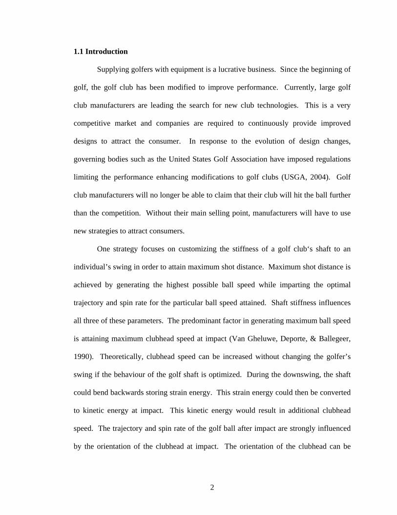
Prior to impact with the ball, the shaft can be measured bending about three

orthogonal axes fixed at the grip end of the club (Fig. 1.2.1.1). The y axis is oriented

from the back to the face of the clubhead, and the x axis from the heel to toe of the

clubhead. Twisting about the longitudinal axis (z axis) of the shaft can also occur.

Compared to the magnitude of deflection about the other axes, twisting about the

longitudinal axis has a negligible influence on both the orientation of the clubhead

(Butler & Winfield, 1994) and its velocity at impact and therefore will not be considered

in this thesis. Further, only deflection occurring along the y axis from the back to the

face of the clubhead can contribute to clubhead speed.

4

For the following descriptions, the club should be pictured in its address position

as shown in Figure 1.2.1.1. The term lag will be used to describe the clubhead if it is

deflected in the negative y direction relative to the neutral shaft position. The term lead

will be used to describe the clubhead if it is deflected in the positive y direction relative

to the neutral shaft position (Fig. 1.2.1.1). Although shaft deflection along the heel/toe

axis cannot contribute to clubhead speed, it can have an influence on ball flight

trajectory. The term toe-down will be used to describe the clubhead if it is deflected in

the negative x direction relative to the neutral shaft position. This is often referred to as

droop in the golfing literature. The term toe-up will be used to describe the clubhead if

it is deflected in the positive x direction relative to the neutral shaft position. It should

z z

x y

Lead Deflection

Toe-down Deflection

Figure 1.2.1.1 Shaft deflection in the lead and toe-down directions.

5

be emphasized that these conventions are defined relative to a three-dimensional

coordinate axis fixed in the grip end of the club.

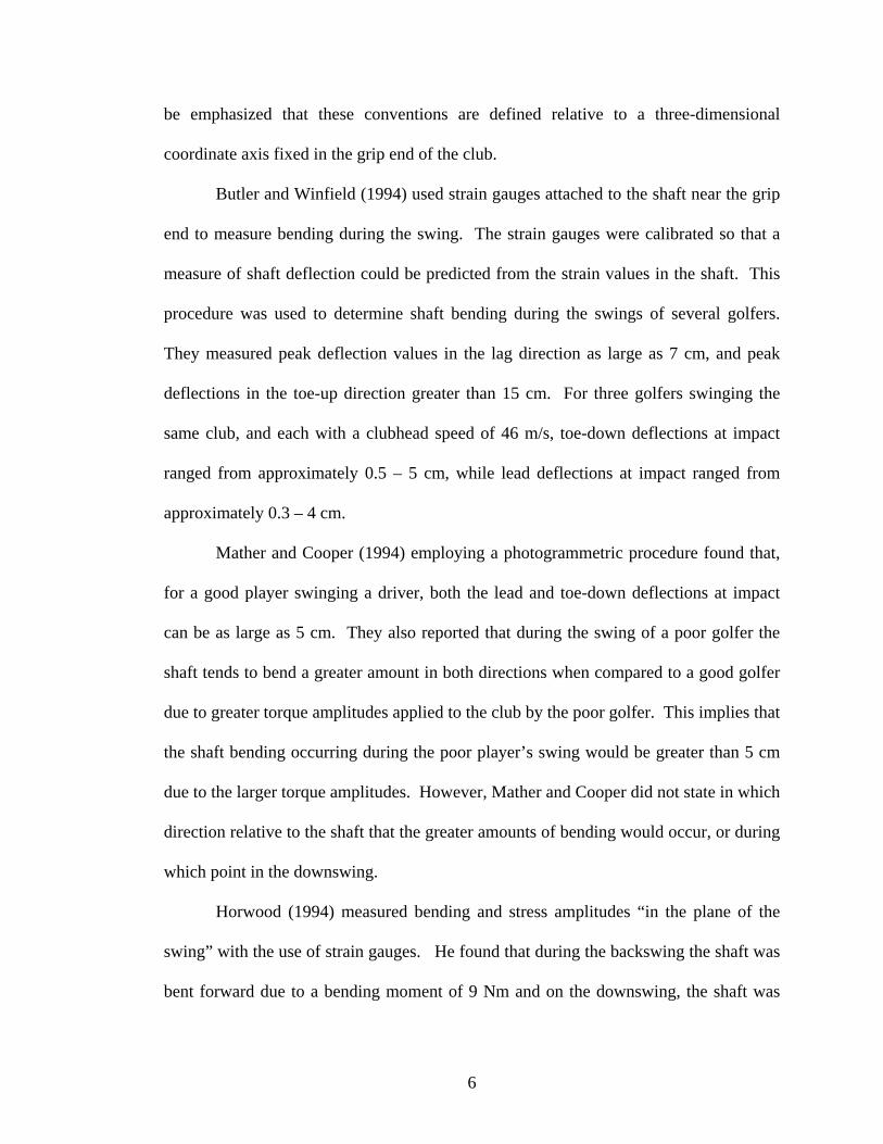
Butler and Winfield (1994) used strain gauges attached to the shaft near the grip

end to measure bending during the swing. The strain gauges were calibrated so that a

measure of shaft deflection could be predicted from the strain values in the shaft. This

procedure was used to determine shaft bending during the swings of several golfers.

They measured peak deflection values in the lag direction as large as 7 cm, and peak

deflections in the toe-up direction greater than 15 cm. For three golfers swinging the

same club, and each with a clubhead speed of 46 m/s, toe-down deflections at impact

ranged from approximately 0.5 – 5 cm, while lead deflections at impact ranged from

approximately 0.3 – 4 cm.

Mather and Cooper (1994) employing a photogrammetric procedure found that,

for a good player swinging a driver, both the lead and toe-down deflections at impact

can be as large as 5 cm. They also reported that during the swing of a poor golfer the

shaft tends to bend a greater amount in both directions when compared to a good golfer

due to greater torque amplitudes applied to the club by the poor golfer. This implies that

the shaft bending occurring during the poor player’s swing would be greater than 5 cm

due to the larger torque amplitudes. However, Mather and Cooper did not state in which

direction relative to the shaft that the greater amounts of bending would occur, or during

which point in the downswing.

Horwood (1994) measured bending and stress amplitudes “in the plane of the

swing” with the use of strain gauges. He found that during the backswing the shaft was

bent forward due to a bending moment of 9 Nm and on the downswing, the shaft was

6

bent backwards due to a bending moment of 6 Nm. Horwood stated that these values

are typical regardless of shaft design or golfer ability. For one golfer swinging an S

(i.e., stiff) flex shaft with a clubhead speed of 42.5 m/s at impact, the clubhead moved

through 12.7 cm from its maximum lagging position into its maximum leading position.

Horwood also stated that the lead deflection present at impact is primarily a function of

centripetal force acting on the offset position of the center of gravity of the head and

inertial forces. Horwood did not go into detail to describe the inertial forces.

There are a few criticisms that can be made regarding Horwood’s (1994)

findings. First, Horwood found that the bending moments in the shaft were greater

during the backswing. It seems doubtful that the bending moments would be greater in

the backswing. Just a qualitative analysis of the golf swing would bring this statement

into question. Second, in opposition to Horwood’s claim that the torque values are

typical regardless of golfer ability; other researchers have found that different golfers

can possess different swing characteristics which would alter the bending moments in

the shaft (Mather & Cooper, 1994; Cooper & Mather, 1994). This will be discussed in

greater detail in a later section. Finally, due to the 90° rotation of the shaft about the

longitudinal axis of the lead arm during the downswing, it is not clear what Horwood

meant by “in the plane of the swing”. The bending moments reported may be in the toe-

up/toe-down direction, or in the lead/lag direction. However, it is likely that Horwood

combined the bending in both directions in some way to determine the bending

occurring in the swing plane.

Perhaps the most cited study regarding the role of the shaft in the golf swing is

that of Milne and Davis (1992). Milne and Davis examined the role of the shaft using

7

both computer simulation and experimental strain gauge measurements. The

presentation of their shaft bending results was ambiguous. One set of sketches,

depicting shaft deformation during the computer simulation, showed maximum

deflections of approximately 2.5 cm, yet a graph of the computer simulation values

clearly showed in-plane deflection values exceeding 10 cm. It is possible that the

discrepancy was due to different measurement conventions for the same phenomenon.

No explanation was given regarding how values for the sketches were measured, but the

paper implies that the deflection values presented in the graph were measured relative to

a tangent to the butt end of the club, thus representing clubhead lead/lag deflection.

This latter technique follows the same convention stated earlier in this thesis regarding

lead/lag and toe-up/toe-down deflections. Milne and Davis presented no deflection

values for the experimental strain gauge data, however, they did present shaft bending

moment data from the live tests which closely agreed with the bending moment data

generated by their simulations. Therefore, it could be interpreted that their live golfer

shaft deflections also reached magnitudes of 10 cm.

Based on the above findings it can be stated that the shaft does bend during the

swing. The exact amount of deformation seems to depend primarily on the swing

pattern generated by the golfer, and in part on the flexibility of the shaft. The bending

occurring in the downswing suggests the shaft can store and release energy, potentially

increasing clubhead speed at impact.

8

1.2.2 Utilization of Energy Stored in the Shaft

When a flexible material, such as a golf shaft composed of graphite or steel is

deformed, potential energy is stored in the material in the form of strain energy. This

energy can be translated into kinetic energy. If this phenomenon does occur during the

down swing, the following sequence would be expected. Early in the downswing, the

golfer applies forces and torques at the grip end of the club that accelerate the club in the

downswing direction. The mass of the clubhead at the distal end of the shaft would

provide an inertial resistance to the motion of the shaft during the downswing. This

inertial resistance would result in shaft bending and the storage of strain energy in the

structure of the shaft. At some point later in the swing, the stored strain energy would

be transferred into kinetic energy and the clubhead would move from lagging behind the

grip end into a leading position. If this happened quickly, just prior to impact, an

increase in clubhead speed over that of a rigid shaft would be expected. This addition to

clubhead speed in the lead direction is referred to as kick velocity.

Milne and Davis (1992) concluded that shaft flexibility does not play an

important dynamic role in the golf swing. It is unclear how this decisive conclusion was

reached. As stated previously, their results suggest the clubhead is deflected

considerably during the downswing, which implies the storage of strain energy and the

possibility of kick velocity adding to the overall clubhead speed. However, there is no

mention of kick velocity in the paper or how the aforementioned bending affects

clubhead speed at all. Certainly, there should be some form of operational definition

that can be used as the measuring stick to determine the importance of shaft flexibility.

Milne and Davis provide no such device. The obvious variable would be kick velocity.

9

It could be stated a priori, that kick velocity needs to exceed a nominal percentage of

total clubhead speed in order for the shaft to be considered as playing an important role

in producing higher ball speed. If this percentage were not reached, then the shaft’s role

in producing higher clubhead speed would be deemed negligible.

There is an important validity concern with the mathematical model developed

by Milne and Davis (1992) that stems from their attempt to model the 3D nature of shaft

dynamics. Milne and Davis realized that an essential requirement of a simulation of

shaft bending was that it be 3D. They stated that the main reason for this is that the

center of mass of the clubhead does not lie on the shaft. Therefore, they “allow” for the

rotation of the clubhead about the longitudinal axis of the lead arm in the plane of the

swing. Although presented in a vague fashion, it appears that clubhead rotation about

the longitudinal axis of the lead arm was incorporated into the simulation in the

following way. From live golfer tests, the distance of the center of mass of the

clubhead from the shaft in the swing plane was determined as a function of the angular

position of the shaft relative to the vertical. The center of mass of the clubhead was then

constrained in their 2D simulations to change its position relative to the shaft as a

function of wrist angle. Although Milne and Davis should be commended for being the

first to make an attempt at representing the 3D nature of the golf swing, I will describe

how their incomplete attempt at 3D modeling inevitably led to their unfounded

conclusion.

Milne and Davis (1992) developed a pseudo-forward dynamics model which

resulted in an incomplete simulation of shaft dynamics during the swing. A true

forward dynamics model would have forces and torques acting as inputs on a system

10

whose inertial properties are sufficiently defined for the number of dimensions that the

system was intended to represent. The kinematics of every point, particle or body will

be completely determined by the input kinetics according to the laws of classical

dynamics. Milne and Davis developed a 2D forward dynamics model in an attempt to

resolve a 3D dynamics problem. The applied torques in the system acted in a single

plane, and the inertial properties of the system’s segments were only expressed for

motion in a single plane. According to classical dynamics, the change in motion of a

body does not occur without the application of a force. In reality, some mechanism

must cause the clubhead to rotate about the longitudinal axis of the lead arm in the plane

of the swing. This mechanism would also have an effect on shaft bending. This

mechanism was not represented in the model employed by Milne and Davis and

therefore its effect on shaft bending cannot be evaluated. A hypothetical thought

experiment will further clarify my point.

Consider the position of a golfer-club system at three-quarters of the way into

the downswing, just as the shaft begins to rotate about the longitudinal axis of the lead

arm through 90° to square up the clubface for impact. At this point, the center of mass

of the clubhead will be at some distance away from the longitudinal axis of the lead arm.

Assume now, that the golfer exerts a torque on the club about the longitudinal axis of

the lead arm in an attempt to square the clubhead for impact. This torque will generate a

bending moment in the shaft and likewise create some magnitude of shaft deflection not

evident in the plane of the swing, but still in the lead/lag direction relative to the

clubface. The dynamic effects of this action on shaft bending cannot be ignored and

will certainly influence shaft deflection in the lead/lag direction as the clubhead moves

11

into a square position at impact. It is precisely a mechanism such as this that cannot be

represented by the model of Milne and Davis.

Therefore Milne and Davis (1992) concluded that shaft bending was solely a

result of centripetal forces acting on an eccentrically placed center of mass. This is not

surprising since their model was not capable of arriving at any other conclusion. In

summary, the study conducted by Milne and Davis lacks the methodological structure to

support their hypothesis and therefore, a sound objective conclusion could not have been

reached with their model.

Miao, Watari, Kawaguchi, and Ikeda (1998) investigated clubhead speed as a

function of grip speed for a variety of shaft flexibility. Three sets of tests were

conducted; computer simulation, robotic, and live golfer. Separate graphs of clubhead

speed versus grip speed were plotted for each shaft flex. For both, the simulation and

machine results, clubhead speed oscillated in a systematic fashion above and below a

line representing the linear relationship between grip speed and clubhead speed

assuming a rigid shaft. For a given grip speed, clubhead speed at impact varied

depending on the shaft stiffness. In the live golfer tests, Miao et al. reported that

clubhead speeds reached a peak at sub maximum grip speed values. On the surface, the

results of Miao et al. seem definitive, however, several criticisms of both their methods

and their interpretation of results can be argued.

The simulation tests conducted by Miao et al. (1998) suffer from the same

limitations as Milne and Davis (1992) in addition to some other concerns. Their

mathematical model is completely 2D in nature and makes no attempt at incorporating

the 90° rotation of the club, about the lead arm, during the downswing. Therefore, the

12

effects of lead/lag deflections occurring prior to and during the rotation of the clubhead

into a square position cannot be represented. Their model has also incorporated two

further assumptions that stem from an attempt to match their simulated data to their

robotic tests. First the acceleration of the grip end of the club was fixed at a constant

value based on the robotic tests. It is doubtful that many golfers accelerate the club at a

constant value during the downswing. Mather and Cooper (1994) showed that the

angular acceleration of the club in the plane of the swing ranged from 0 to

approximately 400 rad/s2 during the downswing. Their second assumption was that the

shaft of the club was considered to have no damping properties. While this assumption

is likely reasonable for a club rigidly fixed at the grip end (such as a robotic test), it is

not so reasonable considering the grip of a live golfer. The hands of the golfer would

certainly introduce some damping into the system (Jorgensen, 1994; Mather & Cooper,

1994; Okubo & Simada, 1990). This concern about the damping effects of a human grip

also applies to their machine tests. It was also not clear if their swing machine

incorporated the rotation of the club about the longitudinal axis of the lead arm during

the downswing. A final point regarding their interpretation of results is directed at their

live golfer tests. Miao et al. (1998) reported that clubhead speeds reached peak values at

sub maximal grip speeds. However, there was no mention of the magnitude of error

associated with their measurement methods. This is especially questionable after

inspection of their scatter plots of grip speed versus clubhead speed. It is evident that

the “peak” clubhead speeds differed from the clubhead speeds attained at the highest

grip speeds by no more than 0.2 m/s. Yet, from these same plots, it is clear that

clubhead speed varied by as much as 3 m/s for a given grip speed with the same club.

13

Since a difference of 0.2 m/s seems to fall within the range of error, the live golfer

results presented by Miao et al. are inconclusive. However, other researchers have

attempted to quantify the actual contribution of kick velocity to clubhead speed at

impact.

Using experimental strain gauge data, Butler and Winfield (1994) calculated

kick velocities at impact that ranged from 2.27 m/s to 2.48 m/s. This was approximately

5% of the total clubhead speed. There appeared to be no obvious relationship between

lead/lag deflection at impact and the corresponding kick velocity reported by Butler and

Winfield. Horwood (1994) had similar findings using strain gauge data. He determined

that the maximum kick velocity was 5% (2.01 m/s) of the total clubhead speed of 42.5

m/s. However, Horwood theorized from his data that kick velocity would not

significantly contribute to clubhead speed. He reasoned that since the clubhead had

close to its largest leading deflection at impact, the kick velocity at this point would be

close to zero. It should be noted that neither of these studies made any attempt to

customize the flex of the golf shafts to the test subjects’ swings. It seems plausible that

if the shaft behaviour was optimized to the individual swings, the kick velocities found

might be higher than 5% and could be timed to occur at impact with the ball.

1.2.3 Variations in Force and Torque Patterns applied to the Club

If all golfers had swings that produced the same kinetic patterns to the golf club,

then only one shaft stiffness would be required for maximized kick velocity. A shaft’s

behaviour is a reflection of the kinetic profile applied throughout the swing. If golfers

swing the club differently, then this results in varying kinetic applications. These varied

14

force and torque applications would result in varied shaft behaviours. However, these

varied shaft behaviours could theoretically be assimilated into the optimized condition,

of attaining maximum kick velocity at impact, by altering shaft stiffness to match the

torque profile of the golfer. Several studies provide evidence that kinetic patterns are

specific to the golfer, and therefore, shaft stiffness can potentially be altered to optimize

kick velocity.

Butler and Winfield (1994) measured the shaft bending profiles of three golfers

using the same club. The profiles were different, yet all swings generated a clubhead

speed of 46 m/s. Three variables measured were load up time, peak deflection, and time

at peak deflection. Load-up time is defined as the time from impact to the start of

loading of the shaft. Peak deflection is the maximum deflection of the shaft in the toe

up/down direction and the time at peak deflection is the amount of time for the shaft to

reach its peak deflection during the downswing. For the three golfers, load up time

ranged from 0.39 s to 0.63 s, peak deflection ranged from 9.2 cm to 15.7 cm, and time at

peak deflection ranged from 0.23 s to 0.51 s. These values indicate that the timing and

amplitude of the kinetics applied by the three golfers are very different. In response to

these different torque patterns, the golf club behaved differently for each golfer.

Other researchers support the contention that golfers swing differently and that

in general, a poor golfer shows greater amplitudes and more fluctuations in torque than a

good golfer (Cooper and Mather, 1994; Mather and Cooper, 1994). According to

Mather et al. (2000) the professional golfer generates as much as 80% of their clubhead

speed in the last stages of the swing. In contrast, the high handicap golfer reaches 120%

of their final impact velocity early in the downswing, slowing appreciably before

15

impact. If this is the case, then a golf shaft will behave differently depending on the

skill of the golfer swinging the club. A good golfer might smoothly accelerate the club,

while a poor golfer would produce acceleration initially, followed by deceleration prior

to impact.

1.2.4 Changes in Clubhead Orientation due to Shaft Deflection

Although it is generally accepted that the orientation of the clubhead relative to

the ball is altered due to shaft bending near impact, very few studies have attempted to

quantify the effects. Mather and Cooper (1994) stated that depending on the geometry

of the shaft, a lead deflection of 5 cm can result in a 5° increase in the loft of the club.

They refer to this added loft as dynamic loft. Horwood (1994) explained that increasing

the lead deflection at impact would increase the dynamic loft at impact and result in a

higher ball trajectory. Although not explicitly reported by any researchers, bending in

the toe-up/toe-down direction will also result in altered ball flight. However, these

effects have not been reported.

1.2.5 Cause of Shaft Bending from a Newtonian Perspective

The resultant force and torque vectors applied by the golfer at the grip end of the

club are continually changing in both magnitude and direction in 3D space during the

downswing. It is solely these two factors, along with gravity, that cause the shaft to

bend during the downswing. To simplify the situation, given a point of rotation, torques

can be replaced by appropriately placed forces without any changes in the dynamics of

the system. Therefore, it can be stated that the forces applied at the grip end of the club

16

are responsible for shaft bending during the downswing. It is my opinion that a clearer

understanding of the source of shaft bending can be gained by resolving the resultant

force, applied at the grip end of the club, into a tangential component and a radial

component. The tangential component would act in a plane formed by the x and y axes,

while the radial component would act along the z axis (Fig. 1.2.1.1).

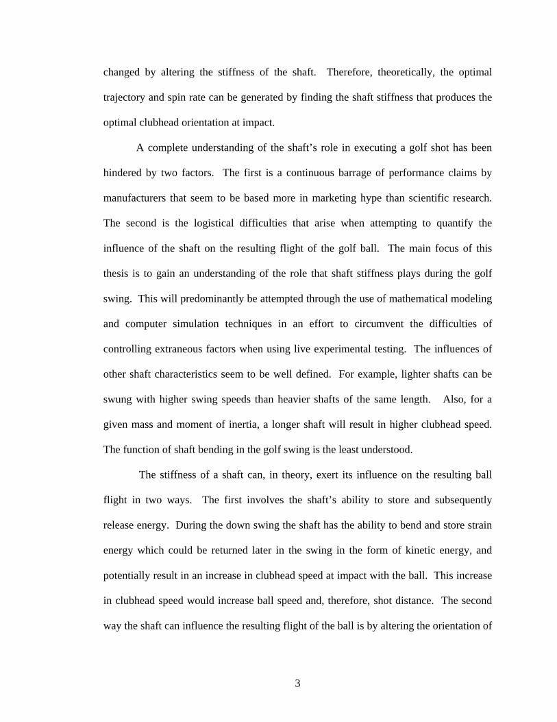
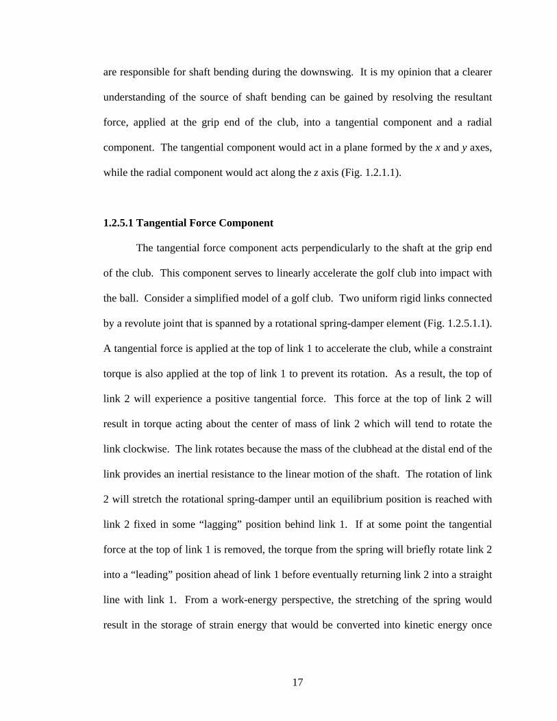
1.2.5.1 Tangential Force Component

The tangential force component acts perpendicularly to the shaft at the grip end

of the club. This component serves to linearly accelerate the golf club into impact with

the ball. Consider a simplified model of a golf club. Two uniform rigid links connected

by a revolute joint that is spanned by a rotational spring-damper element (Fig. 1.2.5.1.1).

A tangential force is applied at the top of link 1 to accelerate the club, while a constraint

torque is also applied at the top of link 1 to prevent its rotation. As a result, the top of

link 2 will experience a positive tangential force. This force at the top of link 2 will

result in torque acting about the center of mass of link 2 which will tend to rotate the

link clockwise. The link rotates because the mass of the clubhead at the distal end of the

link provides an inertial resistance to the linear motion of the shaft. The rotation of link

2 will stretch the rotational spring-damper until an equilibrium position is reached with

link 2 fixed in some “lagging” position behind link 1. If at some point the tangential

force at the top of link 1 is removed, the torque from the spring will briefly rotate link 2

into a “leading” position ahead of link 1 before eventually returning link 2 into a straight

line with link 1. From a work-energy perspective, the stretching of the spring would

result in the storage of strain energy that would be converted into kinetic energy once

17

the tangential force at the top of link 1 was removed. The findings of Miao et al. (1998)

and Jorgensen (1994) were primarily based on the effects of the tangential force applied

at the grip. This was a result of the mathematical models they employed in generating

their findings. Their mathematical models did not incorporate an off-set clubhead center

of mass and therefore, the effects of a radial force component could not have been fully

realized.

Tangential force

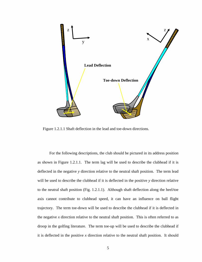
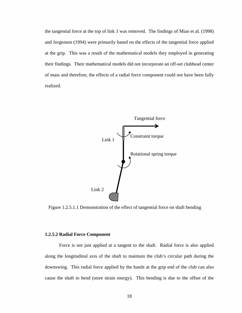
1.2.5.2 Radial Force Component

Force is not just applied at a tangent to the shaft. Radial force is also applied

along the longitudinal axis of the shaft to maintain the club’s circular path during the

downswing. This radial force applied by the hands at the grip end of the club can also

cause the shaft to bend (store strain energy). This bending is due to the offset of the

Link 1 Constraint torque

Rotational spring torque

Link 2

Figure 1.2.5.1.1 Demonstration of the effect of tangential force on shaft bending

18

center of gravity of the clubhead relative to the line of action of the radial force along

the longitudinal axis of the shaft. Consider a similar scenario to the one explained in

section 1.2.5.1. Two uniform rigid links are connected by a revolute joint that is

spanned by a rotational spring-damper element (Fig. 1.2.5.2.1). A vertical (representing

radial) force is applied at the top of link 1 to accelerate the club, while a constraint

torque is also applied at the top of link 1 to prevent its rotation. As a result, the top of

link 2 will experience a positive vertical force. This force at the top of link 2 will result

in torque acting about the center of mass of link 2, due to its offset, which will tend to

rotate the link counter-clockwise. This rotation of link 2 will stretch the rotational

spring-damper until the torque from the spring equals the torque due to the radial force.

Note that it is not possible for the radial force to pull the center of mass of link 2 into a

stable position passed the line of action of the radial force. The nature of this bending

will tend to pull the clubhead into a leading and toe-down position as impact

approaches. An increase in clubhead speed at impact due to the release of this stored

energy is not possible. The strain energy, stored as a result of the radial force, could

only be released prior to impact if the golfer were to let go of the club. Even if the

stored energy could be released, it would result in a negative kick velocity. It should be

noted that the comments in this section describe how the shaft would behave if the radial

force acted in isolation of any tangential force applied to the grip end of the club.

19

Radial force

Constraint torque Link 1

1.2.6 Optimization of Shaft Behaviour

Optimization is a process that results in a best case outcome of a dependent

variable through the manipulation of one or more independent variables. For the

purpose of the golf drive, maximum horizontal clubhead speed at impact is desired (Van

Gheluwe, Deporte, & Ballegeer, 1990). Other factors such as impact quality, ball

launch angle, and ball spin rate also play a role. Theoretically, the shaft can contribute

to clubhead speed by providing a maximum amount of kick velocity at impact. Thus,

shaft behaviour is optimized when the dependent variable, kick velocity, is maximized

at impact.

According to Butler and Winfield (1994), kick velocity is greatest when the shaft

is straight at impact because the kinetic energy is maximized. This statement is in

agreement with the characteristics of an oscillating spring system and is supported by

Link 2

Figure 1.2.5.1.2 Demonstration of the effect of radial force on shaft bending.

Rotational spring torque Line of action of radial force

Center of mass of Link 2

20

other researchers (Horwood, 1994). Jorgensen (1994) in his book ‘The Physics of Golf’

states that the shaft does not have to be straight in order for kick velocity to be

maximized. He determined this through the use of a mathematical model. His

conclusion lacks an adequate description of methodology and a presentation of the

results supporting the claim. Jorgensen also fails to provide a theory for how this

physical phenomenon could occur. One possible explanation of Jorgensen’s finding

could be related to the contribution of shaft bending due to the off-set position of the

clubhead center of mass relative to the shaft. In combination with some ‘spring-back’

effect, this may lead to a kick velocity that increases in magnitude past the mid point of

the shaft’s oscillation. Unfortunately, Jorgensen’s did not incorporate an offset

clubhead center of mass into his model. Jorgensen explained that bending due to the

offset center of mass was a function of centripetal acceleration. He then curiously states

that it will only have an influence early in the swing, while later its effect will be

negligible. He therefore neglects incorporating it into his model.

A second factor that should be considered when optimizing the behaviour of a

shaft is its influence on the orientation of the clubhead at impact with the ball. Based on

the aerodynamics of the golf ball, there will be an optimal launch angle and spin rate

that the ball should possess for it to travel the maximum horizontal distance. The angle

of the clubface, relative to a horizontal line extending to the target, at impact will affect

both the launch angle and spin rate of the golf ball after impact.

21

1.3 Statement of Problem and Hypothesis

1.3.1 The Problem

How does the stiffness of a golf club shaft affect clubhead speed and clubhead

orientation at impact with the ball?

1.3.2 Research Hypotheses

1. A golfer-club system can be simulated with a 3D, six-segment mathematical

model driven by muscle torque generators.

2. Golf shafts bend during the golf swing as a result of both tangential and radial

forces relative to the grip end of the club during the downswing.

3. Customizing the flexibility of a golf shaft to a specific swing will increase

clubhead speed at impact, but not by a meaningful amount (< 1 m/s).

4. Clubhead orientation at impact will depend upon both swing speed and shaft

stiffness.

5. Altering the position of the center of mass of the clubhead relative to the shaft

will affect the dynamics of the golf club during the downswing.

From the review of literature, computer modeling appears to be the best research

tool available to address these hypotheses. The following section will provide a

conceptual understanding and literature review of the modeling methods used in this

thesis.

22

1.4 Review of Optimized Forward Dynamic Simulations

Forward dynamic simulations provide an alternative to researchers attempting to

answer questions about human movement. Forward dynamic simulations offer some

advantages over more traditional methods of human movement inquiry.

One goal for biomechanists is to gain an understanding of how the coordinated

contraction of the body’s muscles can lead to the best execution of a skill. In achieving

this goal the kinematics of the movement must be measured and attempts made at

quantifying the underlying kinetics. A major stumbling block is the error associated

with the techniques biomechanists use in their measurements. Often the associated error

can obscure true measurement values to a point that renders findings inconclusive.

To answer specific questions, the biomechanist might want to measure the effect

of changing one variable while holding all other variables constant. For example, if a

golf swing is perfectly executed every time, what effect will the flexibility of the club’s

shaft have on the resulting clubhead speed at impact? It is difficult for even an elite

performer to execute a skill in an identical manner over many trials. In particular, if

relatively small changes in the outcome are practically significant, then the performer

must have even more precision of repeatability in executing the skill. Further,

considering the golfing example, it is even more difficult for the researcher to know

with certainty that the swing was executed in an identical manner.

A forward dynamics model overcomes some of the issues involved with live

experimentation. Relative to live testing, there is essentially no error in measuring the

outcome of a model, and due to a model’s repeatability in executing a movement; it is

23

very easy to isolate the effects of changing a single variable. However, forward

dynamic models are particularly vulnerable to problems of external validity. In general,

a more detailed model (incorporating more aspects of the real system) is more resilient

to external validity threats. However, a more detailed model is more complex which

inhibits the interpretation of the results. As such, there will always be a subjective

estimate as to the best balance between parsimony, on one side of the scale, and

goodness of fit on the other. It is easier to interpret the results of a simple model, but the

‘correctness’ of those results depend on the validity (internal and external) of the model.

The level of complexity required by a model will depend upon the specific questions the

researcher wants to answer. It is the nature of these questions that should dictate how

the model is developed.

The development of an optimized forward dynamics model can be accomplished

in five phases.

1. Develop the physical properties of each segment

2. Provide the model with the ability to generate motion

3. Develop equations that will govern the motion of the model

4. Determine how the equations will be solved

5. Implement an optimization scheme

The specific methods that were applied in developing the model used in this

thesis may prove to be unnecessarily difficult for the reader to gain a conceptual

understanding of an optimized forward dynamics model. Therefore, the development of

a simpler 2D, 2-segment model will be illustrated. In each of the five phases, the

24

simplest methods, conceptually, will be described, and other techniques previously used

in research will be reviewed.

The development details of a model should be based on the specific question the

researcher wants to answer. In this case, assume the researcher is interested in

determining the optimal muscular control strategy in the execution of a golf swing.

Specifically, what muscle coordination strategy at the shoulder and wrist should a golfer

implement to achieve maximum clubhead velocity at impact with the ball? The purpose

of this section is solely to provide a conceptual framework for optimized forward

dynamic simulations.

1.4.1 Develop the Physical Properties of each Segment

First, the number of segments must be decided. Theoretically, the researcher

should at least include all segments that show motion during execution of the real skill.

However, this could result in motion equations that are too large for the current

capabilities of standard desktop computers, and/or optimization search times that are not

practical. Therefore, the researcher must make certain concessions based on educated

assumptions. For example, the assumption could be made that the motion of the lower

body and trunk has little influence on the muscle control strategy used at the shoulder

and wrist. Although this may not be a realistic assumption, it allows the golfer to be

represented by a model employing just the lead upper arm, forearm, and club. This

supposition allows the model to be reduced to three segments. Perhaps, the researcher

notices that during an actual golf swing, the forearm has no motion relative to the upper

arm. This permits a second assumption, that the forearm and upper arm could be

25

modeled together as a single segment. The model has now been reduced to two

segments. The researcher must decide on the degrees of freedom that each segment of

the model should possess.

The specific degrees of freedom chosen, will dictate whether the system can be

modeled in 2D or 3D. The added complexity of a 3D model over a 2D model cannot be

overstated. If a question can be answered with a 2D model, then a 3D model should not

be employed just for the sake of comprehensiveness. Although it is likely that a golf

swing does not occur perfectly in a single plane, it could be assumed that its deviation

from a plane is not large enough to warrant the added complexity of a 3D simulation.

Therefore, even though, an actual shoulder joint has three degrees of freedom, and a

wrist joint has two degrees of freedom, their motion during a golf swing only requires a

single degree of freedom from each. The assumption could be made that the motion of

segment 1 (upper arm + forearm) and segment 2 (golf club) are both constrained to a

single plane.

The decision on the model’s degrees of freedom allows the inertial parameters of

each segment to be estimated. Since only a 2D representation of the model is required,

each segment can be represented by a single moment of inertia value that corresponds to

an axis perpendicular to the plane of motion. If a segment moved in 3D, then the

moment of inertia must be represented about all three of the segment’s principal axes.

Lengths, masses, and distances to the center of mass for each segment must also be

defined. There are several ways to calculate these physical characteristics for each

segment.

26

The easiest method for obtaining the necessary physical properties of segments

is to simply refer to a reference that directly supplies these values in the form of means

and standard deviations for a large group of individuals. Zatsiorsky (2002) supplies

such data in tabular form. If the researcher wants to make some attempt at basing the

segment’s inertial properties on a particular individual, then regression equations based

on the height and/or weight of an individual are also available (De Leva, 1996). The

potential of more accurate inertial estimates of individuals is provided by the means of

geometrical modeling (Hanavan, 1964; Hatze, 1980; Yeadon, 1990). Employing these

methods, the body is broken down into segments that are represented as geometrical

solids. Measurements are taken on actual individuals to determine the size and shape of

each segment. Density values taken from the literature are then used to calculate

moment of inertia values for each segment.

Suppose we are not interested in our model exactly representing a specific

individual, and that we are satisfied with the knowledge that our model’s physical

properties easily fit within the norms of the human population. Therefore, an arbitrary

golfer is chosen and three measurements are taken: height, mass, and arm length. Based

on these measurements, regression equations are used to determine the moment of

inertia and the position of the arm segment’s center of mass relative to its proximal end

(Table 1.4.1.1). Our model may not exactly represent the particular individual but its

inertial values are certainly a reasonable approximation of the athlete’s inertial

characteristics for their arm. The physical properties for the golf club can be determined

experimentally. Now that we have a physical representation of our model, we must

provide our model with a means for motion.

27

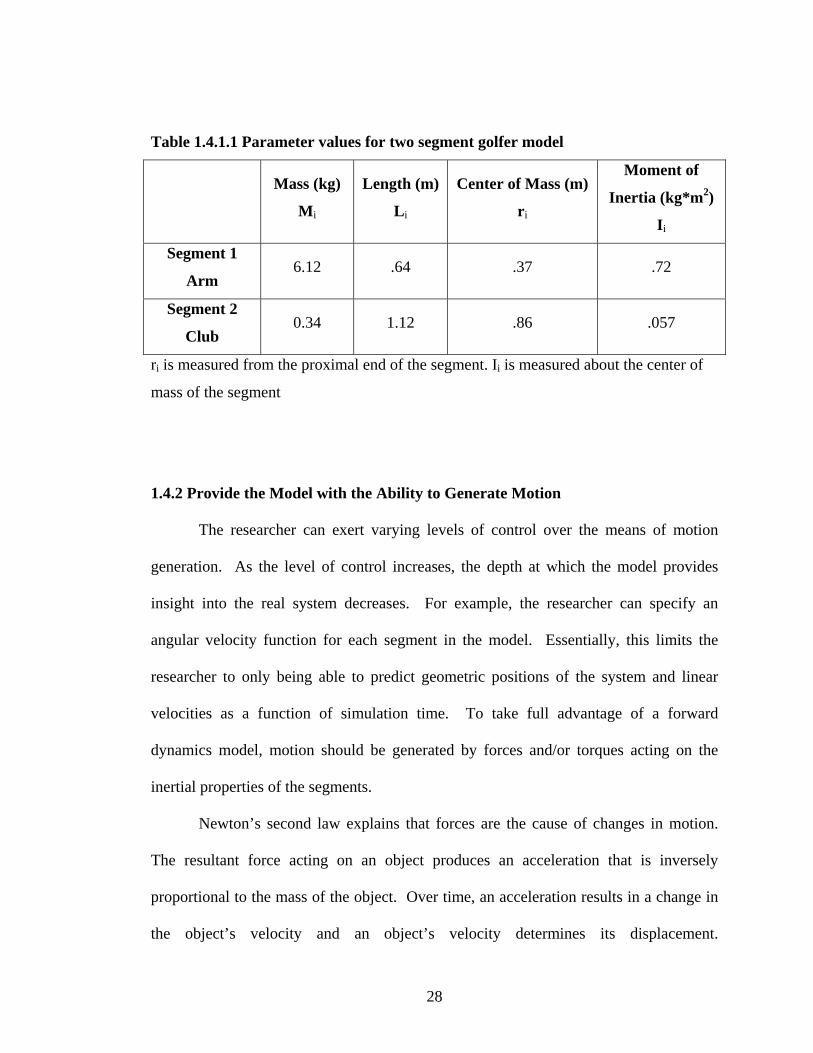
Table 1.4.1.1 Parameter values for two segment golfer model

Mass (kg)

Mi

Length (m)

Li

Center of Mass (m)

ri

Moment of

Inertia (kg*m2)

Ii

Segment 1

Arm 6.12 .64 .37 .72

Segment 2

Club 0.34 1.12 .86 .057

ri is measured from the proximal end of the segment. Ii is measured about the center of

mass of the segment

1.4.2 Provide the Model with the Ability to Generate Motion

The researcher can exert varying levels of control over the means of motion

generation. As the level of control increases, the depth at which the model provides

insight into the real system decreases. For example, the researcher can specify an

angular velocity function for each segment in the model. Essentially, this limits the

researcher to only being able to predict geometric positions of the system and linear

velocities as a function of simulation time. To take full advantage of a forward

dynamics model, motion should be generated by forces and/or torques acting on the

inertial properties of the segments.

Newton’s second law explains that forces are the cause of changes in motion.

The resultant force acting on an object produces an acceleration that is inversely

proportional to the mass of the object. Over time, an acceleration results in a change in

the object’s velocity and an object’s velocity determines its displacement.

28

Conceptually, the same ideas hold true for angular kinetics and kinematics. The

preceding statements in this paragraph are the foundation of forward dynamics. Aside

from gravity, only the muscular activity at the shoulder and wrist will have the ability to

provide energy for the golfer model through the generation of forces and/or torques.

Forces and/or torques can be represented in a forward dynamics model with varying

degrees of complexity.

At the simplest level, it is possible to represent the combined muscle actions at a

joint with a single torque. Theoretically, this torque will produce the same motion as the

combined effect of all individual muscles acting across the joint. A further

simplification would be to assume that once activated, this joint torque instantaneously

rises to its maximum value and remains at this value until it is deactivated. Similarly,

constant muscle forces from individual muscles could be represented if the model was

also provided with estimates for the muscle moment arm lengths. At this level of

complexity, aside from estimating maximal force or torque values, no attempt is made at

representing the behaviour of human muscle.

It has been previously determined that the tendon tension produced by a muscle

depends on four factors: activation level, sarcomere length, velocity of muscle

contraction, and previous contraction history. The level of muscle activation is time

dependent. Essentially, it takes skeletal muscle a certain amount of time to reach its

maximum potential force (Dudel, 1978). The amount of force production capable from

a muscle also depends upon its length, or more specifically, the length of the sarcomeres

that comprise the muscle. This can be explained using the sliding filament theory

(Gordon, Huxley, & Julian, 1966) which contends that maximal force occurs at a

29

sarcomere’s resting length when actin and myosin are optimally overlapped. In practice,

it is difficult to determine at what joint configuration an individual muscle’s sarcomeres

are at resting length. Wilkie (1949) demonstrated that muscle force production was also

a function of a muscle’s rate of shortening. For concentric contractions, a muscle is

capable of producing the most force at slow contraction velocities, while for eccentric

contractions the greatest forces are produced at high contraction velocities. It has been

demonstrated by Cavagna (1974) and Edman (1978) that a muscle will produce a greater

concentric force of contraction if the muscle is immediately put on stretch prior to the

concentric motion. This is referred to as the force enhancement phenomenon.

Previously, researchers have attempted to incorporate these measured muscle behaviours

into their forward dynamic models.

The most popular approach to modeling the aforementioned behaviours has been

through the use of Hill-type muscle models (Hill, 1938; Hill, 1970; Houk, 1963;

Sprigings, 1986; Caldwell, 1995). The majority of Hill models are two-component

mathematical representations of muscle. The model consists of a contractile component

(CC) and a series elastic component (SEC). Although there are no specific anatomical

correlates to these components, the CC can be thought to represent the force producing

muscles fibres, while the SEC mainly corresponds to the tendon. The SEC serves to

modulate the force of the contractile component via its passive force-extension

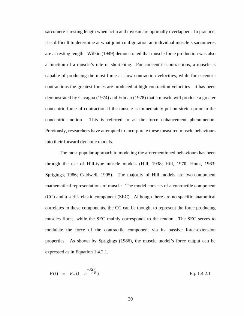
properties. As shown by Sprigings (1986), the muscle model’s force output can be

expressed as in Equation 1.4.2.1.

1.4.2.1 Eq. )1()( BKt

m eFtF−

−=

30

Where,

Fm = maximum isometric force of the represented muscle

K = Hookean spring stiffness

B = damping coefficient of viscosity

t = total time of maximal muscle activation

This basic two-component Hill model incorporates the activation rate property of

muscle, but further additions must be made to model the additional three behaviours.

Incorporating the length-tension characteristics of muscle can be accomplished by

calculating Fm as a function of resting length. Caldwell (1995) determined Fm as a

symmetrical parabolic function of muscle length. Maximum isometric force was

produced when the model was at 100% of its resting length. Fm fell to zero at both 60

and 140% of resting length. Caldwell’s model was not designed to represent a specific

muscle. If detailed experimental data on the force-length characteristics of a specific

muscle were known, then a tailored force-length function could be formulated.

The force-velocity property of muscle can be incorporated by scaling the value

of F(t) after the activation rate and force-length characteristics have been factored into

the muscle model. According to methods used by Alexander (1990) in his model of

human jumping, the following equation (Eq. 1.4.2.2) calculates a new value of force

output (F(t)new) based on the muscle’s current rate of shortening.

F(t)new = F(t) * ( ( Vmax – V) / ( Vmax + G*V ) ) Eq. 1.4.2.2

Where,

31

Vmax = the muscle’s maximum unloaded rate of shortening

V = the muscle’s current rate of shortening

G = a constant

Sprigings (1986) successfully demonstrated that the force enhancement

phenomenon of muscle could be modeled using the two-component Hill model

described above. In order to simulate force enhancement, the Hill model required that

the pre-stretch of the muscle be entered as an input function. Capturing the force

enhancement behaviour has also been attempted by altering the value of Fm (Alexander,

1990). Instead of using the maximum isometric force capable of a muscle, Alexander

employed the larger maximum eccentric force capability.

It has been previously stated that, for the purposes of section 1.4, the simplest

methods in each of the model’s development phases would be used. The most

straightforward method of powering the 2D, 2-segment golfer model is through the use

of constant torques. Therefore, for the conceptual model under development in this

section, torque actuators will be inserted at the proximal end of each segment. The

actuators will represent the sum of all muscle action across each joint. In their activated

state, the actuators will produce constant values equivalent to the maximum torques

possible at both the shoulder (150 N) and wrist (40 N).

1.4.3 Develop Equations that will Govern the Motion of the Model

It is in this phase of development that the principles of classical dynamics are

imposed on the golfer model. There are only a few methods that are used to develop

these equations and at the heart of each method are the basic mechanical principles.

32

Generally, the equations are formulated from either an impulse-momentum framework

or a work-energy perspective. Each of the methods has its advantages and

disadvantages, but the questions that are asked of the model will dictate which method is

best suited for the development of the equations of motion. The methods can be loosely

grouped into Newton, D’Alambert, Lagrange, Hamilton, and Kane formulations.

The Newtonian method is based on creating a free-body diagram for every

segment in the model and applying the standard ΣF=ma and ΣT=Iα equations. Motion

is assumed to be occurring in an inertial reference frame and the center of mass for each

segment serves as the point to sum the moments. For the individual with only a basic

knowledge of mechanics and mathematics, the Newtonian method is conceptually the

simplest. Since each segment is dealt with individually, a deeper understanding of the

system’s mechanics can be garnered. However, the method compels the resolution of

all inter-segmental forces whether they are desired or not. This inevitably leads to much

lengthier motion equations than required if only the kinematics and external forces of

the system were of interest. In an attempt to simplify the complexities of dynamics,

D’Alembert’s method considers the inertial terms “ma” as a force and moves it to the

left side of the equation allowing a dynamic problem to be solved statically (Yamaguchi,

2001). This simplifies the situation mathematically, but results in fictitious forces and

thus the potential for confusion of the underlying mechanics. However, D’Alembert’s

method can be applied in a non-inertial setting. This results in potentially shorter

equations of motion in comparison to the Newtonian method.

An alternative to the Newtonian formulation is the Lagrangian method for

developing the equations of motion. While still based on Newton’s Laws of Motion, the

33

Lagrangian method focuses on the total amount of physical energy in the system. The

Lagrangian is defined as the difference between the kinetic and potential energy of the

system (Andrews, 1995). Unlike the Newtonian method, the Lagrangian approach does

not determine the inter-segmental forces, and therefore generates more compact

equations of motion. However, the Lagrangian method still produces n second order

equations for an n degree of freedom model. For a model comprised of as little as 4

segments moving in 3D, the second order equations become complex and difficult to

solve. The Hamiltonian formulation which uses the Lagrangian formulation as its

starting point overcomes this difficulty. By applying a Legendre transformation to the

Lagrangian formulation, the equations of motion for an n degree of freedom model can

be expressed by 2n first order differential equations (Hogarth, 2002). This

transformation results in the Hamiltonian formulation representing the generalized

momenta of the system. However, if certain inter-segmental forces are desired, then the

Hamiltonian approach, like its Lagrangian precursor, is not suitable.

Although researchers had a sound understanding of classical mechanics for at

least a couple of centuries prior to the advent of the computer, few attempts were made

at solving the equations of motions for multi-body system. When brute computational

power became available, the methods previously described to develop the equations of

motion were put to use. Even taking into account the considerable leaps in computing

power over the past 50 years, the computational efficiency for a set of motion equations

is still an issue. Kane’s method for developing the equations of motion for rigid body

systems greatly improves the computational efficiency of forward dynamic models

(Mitiguy & Kane, 1996).

34

As a starting point, Kane’s method is based on D’Alembert’s reformulation of

Newton’s second law. Kane’s method differs from the other traditional methods.

According to Yamaguchi (2001),

“…Kane’s Method views the system together as a whole, creates auxiliary

quantities called partial angular velocities and partial velocities, and uses

them to form dot products from quantities called the generalized active

forces and generalized inertia forces, which are simplified forms of the

forces and moments used to write the dynamic equations of motion. It is in

forming these dot products that the main advantage of Kane’s Method

becomes apparent, because only the forces and torques that actually create

motion will survive.”

Kane’s method results in n first order dynamic equations describing the motions of a

system with n degrees of freedom. If specific inter-segmental forces and torques are of

interest, then they can be determined by generating expressions for them in the same

manner as the expressions for the other generalized forces. Kane’s systematic

mathematical treatment of Newton’s laws makes his method computationally superior

for use in forward dynamic applications. However, the same attributes that makes

Kane’s method computationally superior, also make it conceptually more challenging

than the Newtonian formulation. Therefore, for the basic conceptual purposes of this

section, the equations of motion for the 2D golfer model will be developed using a

Newtonian formulation.

The Newtonian method is initiated by determining the kinematic equations of

motion for the model. These equations are also referred to as constraint equations, as

35

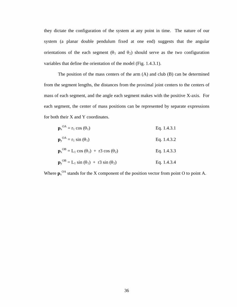
they dictate the configuration of the system at any point in time. The nature of our

system (a planar double pendulum fixed at one end) suggests that the angular

orientations of the each segment (θ1 and θ2) should serve as the two configuration

variables that define the orientation of the model (Fig. 1.4.3.1).

The position of the mass centers of the arm (A) and club (B) can be determined

from the segment lengths, the distances from the proximal joint centers to the centers of

mass of each segment, and the angle each segment makes with the positive X-axis. For

each segment, the center of mass positions can be represented by separate expressions

for both their X and Y coordinates.

pxOA = r1 cos (θ1) Eq. 1.4.3.1

pyOA = r1 sin (θ1) Eq. 1.4.3.2

pxOB = L1 cos (θ1) + r3 cos (θ2) Eq. 1.4.3.3

pyOB = L1 sin (θ1) + r3 sin (θ2) Eq. 1.4.3.4

Where pxOA stands for the X component of the position vector from point O to point A.

36

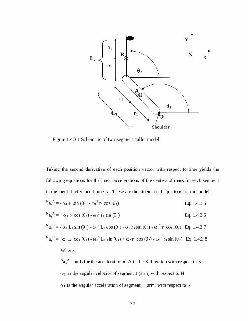
Taking the second derivative of each position vector with respect to time yields the

following equations for the linear accelerations of the centers of mass for each segment

in the inertial reference frame N. These are the kinematical equations for the model.

NaxA = - α1 r1 sin (θ1) - ω1

2 r1 cos (θ1) Eq. 1.4.3.5

NayA = α1 r1 cos (θ1) - ω1

2 r1 sin (θ1) Eq. 1.4.3.6

NaxB = - α1 L1 sin (θ1) - ω1

2 L1 cos (θ1) - α2 r3 sin (θ2) - ω22 r3 cos (θ2) Eq. 1.4.3.7

NayB = α1 L1 cos (θ1) - ω1

2 L1 sin (θ1) + α2 r3 cos (θ2) - ω22 r3 sin (θ2) Eq. 1.4.3.8

Where,

NaxA stands for the acceleration of A in the X direction with respect to N

ω1 is the angular velocity of segment 1 (arm) with respect to N

α1 is the angular acceleration of segment 1 (arm) with respect to N

Shoulder

θ1

θ2

r1L1

r4

r3

r2⊗

L2

A

B

O

Y

N X ⊗

Figure 1.4.3.1 Schematic of two-segment golfer model.

37

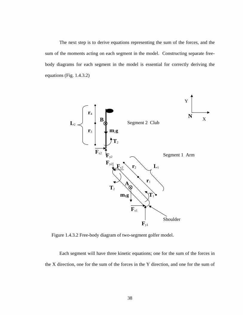
The next step is to derive equations representing the sum of the forces, and the

sum of the moments acting on each segment in the model. Constructing separate free-

body diagrams for each segment in the model is essential for correctly deriving the

equations (Fig. 1.4.3.2)

Each segment will have three kinetic equations; one for the sum of the forces in

the X direction, one for the sum of the forces in the Y direction, and one for the sum of

r4

r3

⊗L2B

r1

L1r2

⊗A

Y

X N Segment 2 Club

m2g

T2

Fx2 Fy2 Segment 1 Arm

Fx1

Fy1

m1g T1

Fy2 Fx2

T2

Shoulder

Figure 1.4.3.2 Free-body diagram of two-segment golfer model.

38

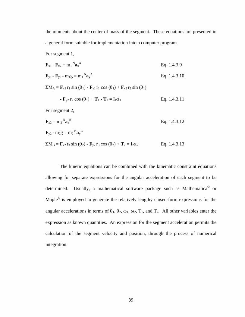
the moments about the center of mass of the segment. These equations are presented in

a general form suitable for implementation into a computer program.

For segment 1,

Fx1 - Fx2 = m1 Nax

A Eq. 1.4.3.9

Fy1 - Fy2 - m1g = m1 Nay

A Eq. 1.4.3.10

ΣMA = Fx1 r1 sin (θ1) - Fy1 r1 cos (θ1) + Fx2 r2 sin (θ1)

- Fy2 r2 cos (θ1) + T1 - T2 = I1α1 Eq. 1.4.3.11

For segment 2,

Fx2 = m2 Nax

B Eq. 1.4.3.12

Fy2 - m2g = m2 Nay

B

ΣMB = Fx2 r3 sin (θ2) - Fy2 r3 cos (θ2) + T2 = I2α2 Eq. 1.4.3.13

The kinetic equations can be combined with the kinematic constraint equations

allowing for separate expressions for the angular acceleration of each segment to be

determined. Usually, a mathematical software package such as Mathematica© or

Maple© is employed to generate the relatively lengthy closed-form expressions for the

angular accelerations in terms of θ1, θ2, ω1, ω2, T1, and T2. All other variables enter the

expression as known quantities. An expression for the segment acceleration permits the

calculation of the segment velocity and position, through the process of numerical

integration.

39

1.4.4 Determine How the Equations will be Solved

For most musculoskeletal models, the equations of motion are a set of second

order differential equations that need to be solved numerically. This is an iterative

process that solves for the corresponding first and zeroth order equations of motion at

each time step. The most straightforward method of numerically solving differential

equations is known as Euler’s method. The following is a description of its

implementation with the 2D model.

Given the chance, muscle torques and gravity will act on the golfer model

resulting in acceleration. In the previous section, expressions were developed for the

angular accelerations of each segment in the model. It is possible to determine angular

acceleration for each segment at t=0 given initial position and velocity data. The total

simulation time for our model, from initiation of movement until impact with the ball,

can be divided up into a series of smaller time intervals. Assuming that the

accelerations determined at t = 0 remain constant during the entire first time interval,

Euler’s method can be used to determine both velocity and displacement at the end of

this interval. These new velocity and displacement values along with new muscle

torques are entered into the equations of motion to determine accelerations for the next

time interval. The following two equations demonstrate how the angular kinematics are

stepped through in a sequential manner.

ωI+1 = ωI + αI∆t Eq. 1.4.4.1

θI+1 = θI + ωI∆t Eq. 1.4.4.2

Where,

I indicates the present time interval

40

I + 1 indicates the next time interval

θ is the angular position

ω is the angular velocity

α is the angular acceleration

∆t is the length of the time interval

This procedure is repeated until a predetermined condition is reached signifying the end

of the simulation such as contact with the ball.

The extension from Euler’s method to other forms of numerical solution is one

of technical sophistication not conception. Two commonly used numerical solution

methods in forward dynamic models are versions of the Runge-Kutta and Kutta-Merson

algorithms. Remember that the Euler method assumed that the acceleration determined

at the start of a time interval remained constant for the duration of that time interval.

This assumption allows the motion equations to be solved a single time for each time

interval. While computationally efficient, it can lead to large errors due to poor

approximation of the ‘true’ acceleration curve. That is, the acceleration curve that

would be generated if infinitely small time intervals were used. Kutta methods attempt

to evaluate how much the acceleration function is changing during the time interval.

This is accomplished by evaluating the motion equations at several points over the time

interval and using an average acceleration. Advanced Kutta algorithms use variable

time intervals throughout the simulation. For example, assume the acceleration function

remained constant for the first half of the simulation and became erratic over the second

half of the simulation. Advanced algorithms would employ large time intervals over the

41

first half and very small time intervals over the second half. This allows a balance

between computational efficiency and accuracy.

The forward dynamics model is now functional. Given specific inputs from the

muscle torque generators the behaviour of the model can be predicted. However, the

goal of the model was to determine the muscle coordination strategy a golfer should

implement to achieve maximum clubhead velocity at impact with the ball. This requires

knowing when to activate the muscle torques and if necessary when to deactivate them.

This knowledge can be gained by optimizing the forward dynamics model.

1.4.5 Implement an Optimization Scheme

Optimization entails maximizing or minimizing the value of a function by

searching for the best combination of that function’s independent variables. In the

context of our research question from section 1.4, clubhead velocity at impact is the

function whose value needs to be maximized. Clubhead velocity at impact is

determined by the muscle control strategy used at the shoulder and wrist during the

downswing. Specifically, the start and duration times for the torque generators at the

shoulder and wrist are the independent or control variables for the optimization. There

exists an optimal pattern of torque generator activation that will lead to maximum

clubhead velocity at impact with the ball. A scheme needs to be employed that will

search for and return the values of the control variables that will generate the optimal

pattern of torque generator activation. It is possible to conduct an optimization by either

maximizing or minimizing a function’s value. Since we are interested in larger

42

clubhead speeds, optimization approaches will only be discussed in the context of

maximizing a function.

To help acquire an understanding of optimization methods, let’s temporarily

consider a simplified scenario under which the golfer model requires optimization.

Assume that the time of onset of the shoulder torque requires no control and is fully

activated throughout the entire simulation. Further, assume that once the wrist torque is

activated, it remains active for the duration of the simulation. This leaves only a single

control variable; the start time for the wrist torque. In this simplified state, clubhead

velocity is only a function of wrist torque start time. In terms of optimization, this is

considered a one-dimensional search space. A hypothetical graph of clubhead velocity

at impact as a function of wrist torque start times is shown in Fig. 1.4.5.1. With only a

single control variable it is easy to visualize the search space. The goal of the

optimization algorithm is to find, as quickly as possible the wrist torque start time

associated with the largest clubhead velocity which is represented by the global

maximum.

43

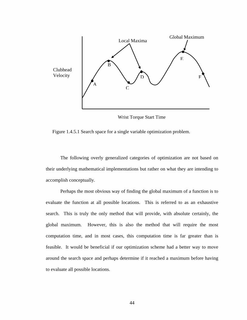
The following overly generalized categories of optimization are not based on

their underlying mathematical implementations but rather on what they are intending to

accomplish conceptually.

Perhaps the most obvious way of finding the global maximum of a function is to

evaluate the function at all possible locations. This is referred to as an exhaustive

search. This is truly the only method that will provide, with absolute certainly, the

global maximum. However, this is also the method that will require the most

computation time, and in most cases, this computation time is far greater than is

feasible. It would be beneficial if our optimization scheme had a better way to move

around the search space and perhaps determine if it reached a maximum before having

to evaluate all possible locations.

E

FD

C

B

Wrist Torque Start Time

Clubhead Velocity

Local MaximaGlobal Maximum

A

Figure 1.4.5.1 Search space for a single variable optimization problem.

44

To save on computational time a local search method could be used. The

general schema for a local search algorithm is as follows. Randomly pick a point in the

search space from which to start and evaluate the function at that point. Perform some

transformation to the current point’s coordinates, so that a new point nearby is selected

for evaluation. If the new point has a higher function value, then the new point becomes

the current point. If the new point has a lower function value, then another new point is

selected based on another transformation of the current point’s coordinates. This pattern

is repeated until no improvements in the function’s value can be found from the search’s

current position. When this happens, the function’s value at the current position

becomes the maximum returned by the optimization algorithm. Local searches, such as

the hill-climbing method just described, differ only in how the transformation is applied

to the current position. The problem with hill-climbers and local searches in general, is

that they tend to get trapped on local maximums. Consider the diagram in Fig. 1.4.5.1,

if the search started at point A, then the algorithm would find its way to B and realize

that all nearby points result in smaller function values and conclude that B is the optimal

solution. If the starting point was C, then the search would likely conclude at either B or

D. As you can see, the success of a local search depends on the initial starting point. If

the search started at F, then the algorithm would have serendipitously found the global

maximum at E. This dependency on an initial starting point requires that local search

algorithms must be started several times from random locations in the search space to

have a chance at finding the global maximum. Essentially, the downfall of local

searches is that they don’t have the ability to climb down from relatively short hills.

45

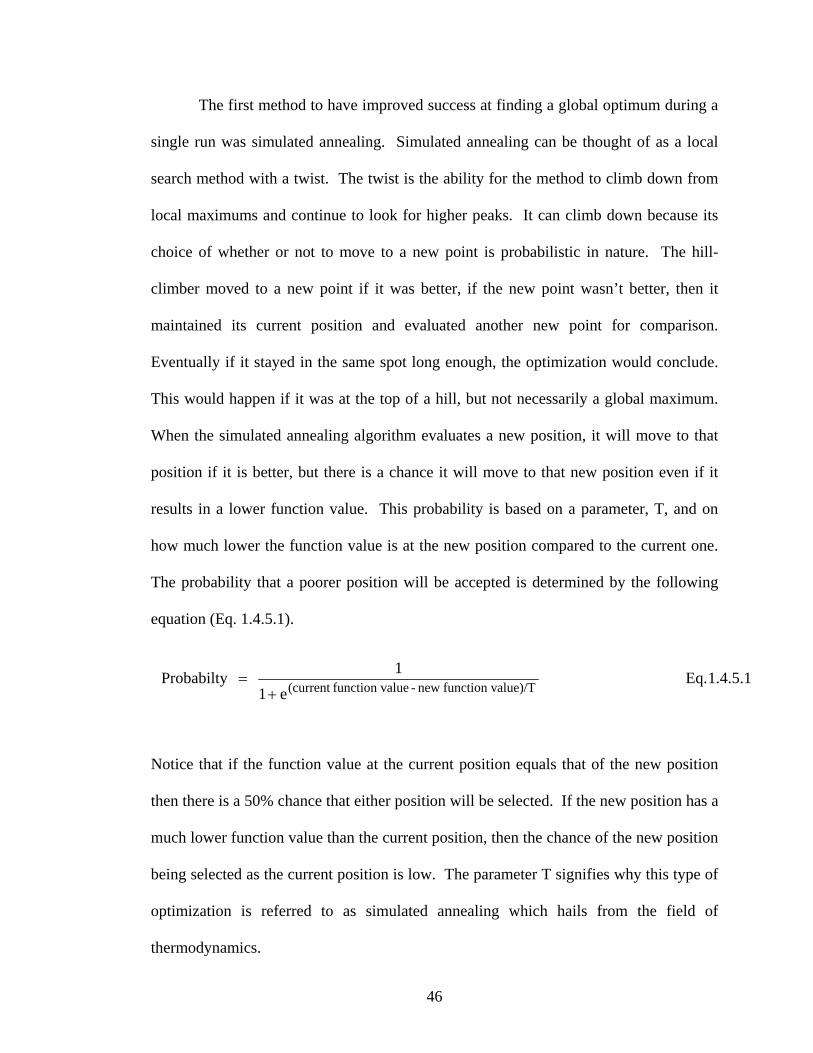
The first method to have improved success at finding a global optimum during a

single run was simulated annealing. Simulated annealing can be thought of as a local

search method with a twist. The twist is the ability for the method to climb down from

local maximums and continue to look for higher peaks. It can climb down because its

choice of whether or not to move to a new point is probabilistic in nature. The hill-

climber moved to a new point if it was better, if the new point wasn’t better, then it

maintained its current position and evaluated another new point for comparison.

Eventually if it stayed in the same spot long enough, the optimization would conclude.

This would happen if it was at the top of a hill, but not necessarily a global maximum.

When the simulated annealing algorithm evaluates a new position, it will move to that

position if it is better, but there is a chance it will move to that new position even if it

results in a lower function value. This probability is based on a parameter, T, and on

how much lower the function value is at the new position compared to the current one.

The probability that a poorer position will be accepted is determined by the following

equation (Eq. 1.4.5.1).

1.4.5.1 Eq. e 1

1 Probabilty alue)/Tfunction v new - aluefunction v(current +=

Notice that if the function value at the current position equals that of the new position

then there is a 50% chance that either position will be selected. If the new position has a

much lower function value than the current position, then the chance of the new position

being selected as the current position is low. The parameter T signifies why this type of

optimization is referred to as simulated annealing which hails from the field of

thermodynamics.

46

To grow a crystal, you want to start with the material in a very hot liquid state

and slowly cool the substance until it becomes locked into a crystal form. Problems

occur

loped that

allow a

if the liquid is cooled to quickly. If cooled quickly, the crystal will have

irregularities and the energy level is higher than a perfectly ordered crystal. The control

parameter T signifies the rate at which the solution to the optimization is “cooled”. The

variable T essentially controls the ability of the algorithm to climb down from peaks. At

the start of the optimization, T is large and the simulated annealing algorithm behaves

like a random search, as the temperature cools (T decreases in value) new points that are

worse than the current point have less chance on being selected. Near the end of the

optimization, the simulated annealing algorithm behaves like a regular hill-climber, but

hopefully, the previous iterations have led it to the hill with the highest peak.

The three optimization methods discussed thus far evaluate a single solution to

the optimization during each iteration. Optimization methods have been deve

population of solutions to be evaluated at each step during the optimization.

This branch of optimization has been referred to as genetic or evolutionary

programming. From the initial statements in this paragraph, it might appear as though

an evolutionary program could simply be several hill-climbers, or simulated annealing

programs running at the same time. This would be no more successful than repeating

the optimization scheme several times, and accepting the best answer found. However,

evolutionary programs actually have the solutions competing and interacting with each

other during every iteration of the optimization. Based on Darwin’s theories of

evolution, solutions compete against each other and the fittest individuals have the best

chance of surviving to pass on their attributes to future generations. In addition, just like

47

in natural evolution, a random mutation component can be added to the solutions that

survive into the next generation (iteration). Suppose that 6 points (each point represents

an individual) were randomly picked for evaluation from the search space shown in

Figure 1.4.5.1. After evaluation each individual was given a chance on being selected to

survive into the next iteration (generation). The magnitude of the probability of being

selected is directly proportional to their fitness (function value at that point) relative to

all the other individuals. For example, if Individual #1 had a fitness of 45 m/s, and the

sum of all six individuals’ fitness values was 90 m/s, then Individual #1 would have a 50

% (45/90) chance of being selected. Each individual is given a slot on a roulette wheel

whose area is proportional to their relative fitness, i.e. Individual #1’s area occupies

50% of the roulette wheel. In selecting 6 individuals that will survive into the next

generation, the roulette wheel is spun 6 times. If the die lands in a particular

individual’s space, then that individual survives. This system allows really fit

individuals to be selected more than once. Once selected, their genetic code (the control

variables), or in this case wrist torque start time is mutated, and these mutated

individuals are evaluated in the next generation.

An evolutionary optimization scheme was employed in the development and

implementation of the model used in this thesis. Since evolutionary programming is

concep

the methods that were used in the development of the

golfer model used in this thesis will describe only the finer points of the methods and

tually straightforward, a more detailed discussion on the program’s structure will

be saved until the next chapter.

This concludes the general explanation and review of forward dynamic

simulations. The description of

48

not how the methods actually work or were employed. The reader should refer back to

this chapter for conceptual insight into the specific workings of an optimized forward

dynamics model.

49

2

METHODS

50

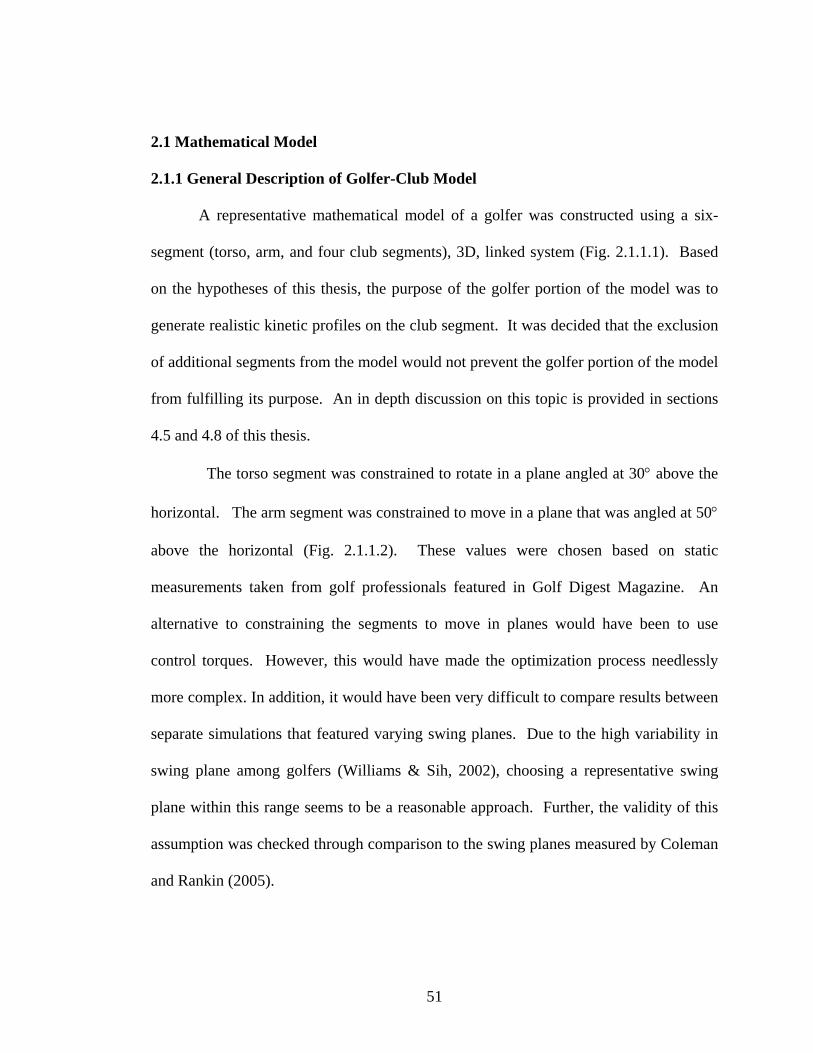
2.1 Mathematical Model

2.1.1 General Description of Golfer-Club Model

A representative mathematical model of a golfer was constructed using a six-

segment (torso, arm, and four club segments), 3D, linked system (Fig. 2.1.1.1). Based

on the hypotheses of this thesis, the purpose of the golfer portion of the model was to

generate realistic kinetic profiles on the club segment. It was decided that the exclusion

of additional segments from the model would not prevent the golfer portion of the model

from fulfilling its purpose. An in depth discussion on this topic is provided in sections

4.5 and 4.8 of this thesis.

The torso segment was constrained to rotate in a plane angled at 30° above the

horizontal. The arm segment was constrained to move in a plane that was angled at 50°

above the horizontal (Fig. 2.1.1.2). These values were chosen based on static

measurements taken from golf professionals featured in Golf Digest Magazine. An

alternative to constraining the segments to move in planes would have been to use

control torques. However, this would have made the optimization process needlessly

more complex. In addition, it would have been very difficult to compare results between

separate simulations that featured varying swing planes. Due to the high variability in

swing plane among golfers (Williams & Sih, 2002), choosing a representative swing

plane within this range seems to be a reasonable approach. Further, the validity of this

assumption was checked through comparison to the swing planes measured by Coleman

and Rankin (2005).

51

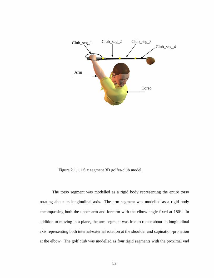
Club_seg_2 Club_seg_3 Club_seg_1Club_seg_4

The torso segment was modelled as a rigid body representing the entire torso

rotating about its longitudinal axis. The arm segment was modelled as a rigid body

encompassing both the upper arm and forearm with the elbow angle fixed at 180°. In

addition to moving in a plane, the arm segment was free to rotate about its longitudinal

axis representing both internal-external rotation at the shoulder and supination-pronation

at the elbow. The golf club was modelled as four rigid segments with the proximal end

Torso

Arm

Figure 2.1.1.1 Six segment 3D golfer-club model.

52

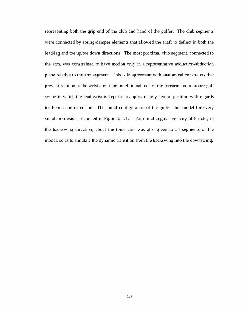
representing both the grip end of the club and hand of the golfer. The club segments

were connected by spring-damper elements that allowed the shaft to deflect in both the

lead/lag and toe up/toe down directions. The most proximal club segment, connected to

the arm, was constrained to have motion only in a representative adduction-abduction

plane relative to the arm segment. This is in agreement with anatomical constraints that

prevent rotation at the wrist about the longitudinal axis of the forearm and a proper golf

swing in which the lead wrist is kept in an approximately neutral position with regards

to flexion and extension. The initial configuration of the golfer-club model for every

simulation was as depicted in Figure 2.1.1.1. An initial angular velocity of 5 rad/s, in

the backswing direction, about the torso axis was also given to all segments of the

model, so as to simulate the dynamic transition from the backswing into the downswing.

53

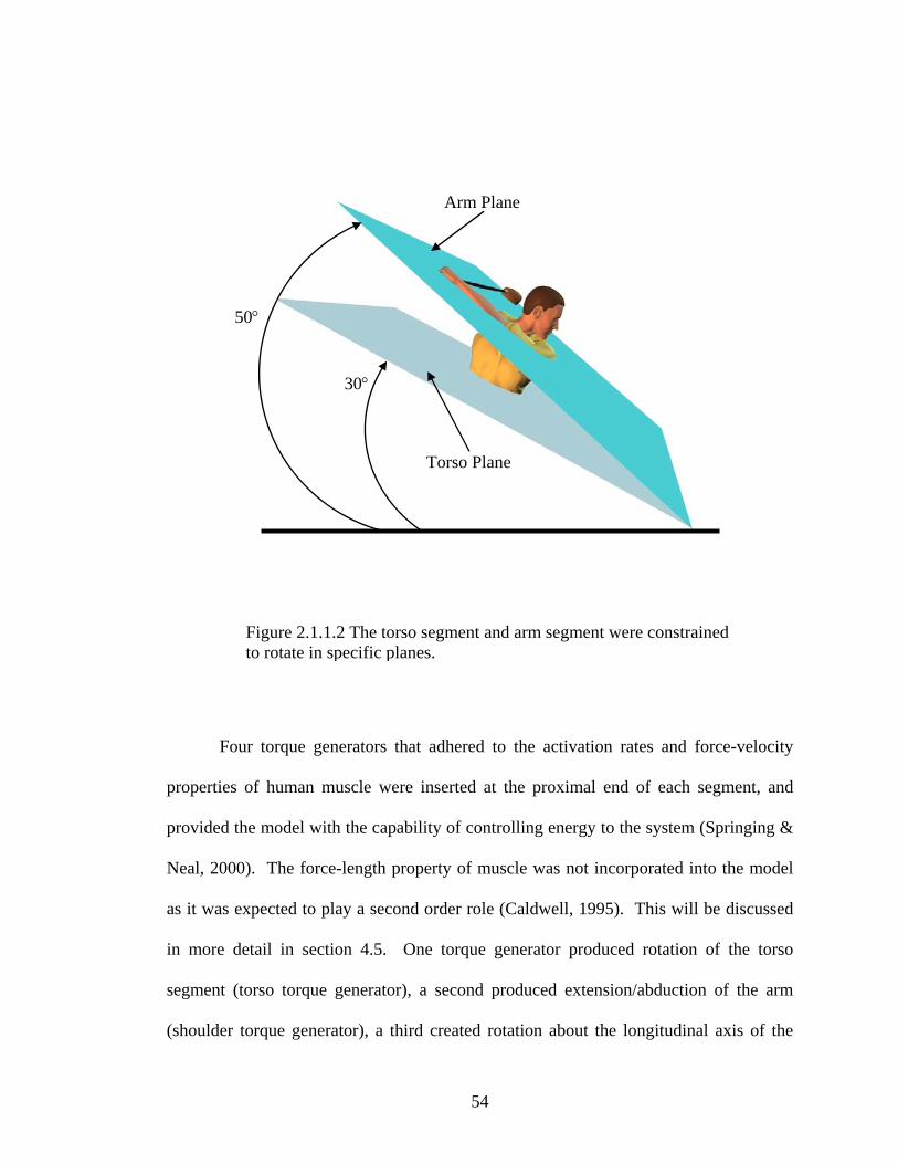
Arm Plane

Four torque generators that adhered to the activation rates and force-velocity

properties of human muscle were inserted at the proximal end of each segment, and

provided the model with the capability of controlling energy to the system (Springing &

Neal, 2000). The force-length property of muscle was not incorporated into the model

as it was expected to play a second order role (Caldwell, 1995). This will be discussed

in more detail in section 4.5. One torque generator produced rotation of the torso

segment (torso torque generator), a second produced extension/abduction of the arm

(shoulder torque generator), a third created rotation about the longitudinal axis of the

30°

50°

Torso Plane

Figure 2.1.1.2 The torso segment and arm segment were constrained to rotate in specific planes.

54

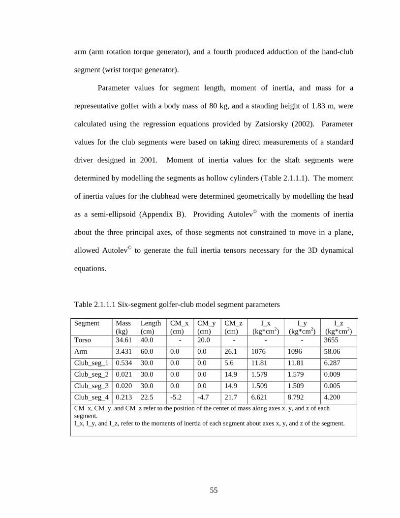
arm (arm rotation torque generator), and a fourth produced adduction of the hand-club

segment (wrist torque generator).

Parameter values for segment length, moment of inertia, and mass for a

representative golfer with a body mass of 80 kg, and a standing height of 1.83 m, were

calculated using the regression equations provided by Zatsiorsky (2002). Parameter

values for the club segments were based on taking direct measurements of a standard

driver designed in 2001. Moment of inertia values for the shaft segments were

determined by modelling the segments as hollow cylinders (Table 2.1.1.1). The moment

of inertia values for the clubhead were determined geometrically by modelling the head

as a semi-ellipsoid (Appendix B). Providing Autolev© with the moments of inertia

about the three principal axes, of those segments not constrained to move in a plane,

allowed Autolev© to generate the full inertia tensors necessary for the 3D dynamical

equations.

Table 2.1.1.1 Six-segment golfer-club model segment parameters

Segment Mass (kg)

Length (cm)

CM_x (cm)

CM_y (cm)

CM_z (cm)

I_x (kg*cm2)

I_y (kg*cm2)

I_z (kg*cm2)

Torso 34.61 40.0 - 20.0 - - - 3655 Arm 3.431 60.0 0.0 0.0 26.1 1076 1096 58.06 Club_seg_1 0.534 30.0 0.0 0.0 5.6 11.81 11.81 6.287 Club_seg_2 0.021 30.0 0.0 0.0 14.9 1.579 1.579 0.009 Club_seg_3 0.020 30.0 0.0 0.0 14.9 1.509 1.509 0.005 Club_seg_4 0.213 22.5 -5.2 -4.7 21.7 6.621 8.792 4.200 CM_x, CM_y, and CM_z refer to the position of the center of mass along axes x, y, and z of each segment. I_x, I_y, and I_z, refer to the moments of inertia of each segment about axes x, y, and z of the segment.

55

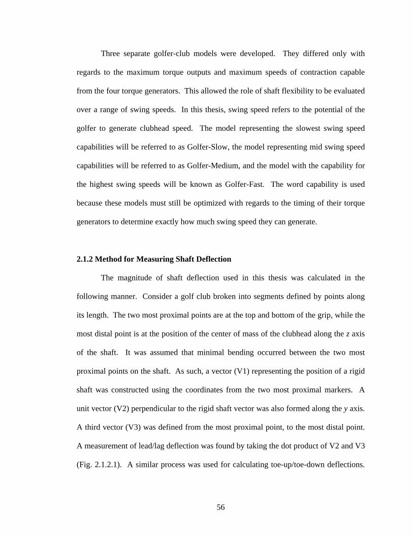
Three separate golfer-club models were developed. They differed only with

regards to the maximum torque outputs and maximum speeds of contraction capable

from the four torque generators. This allowed the role of shaft flexibility to be evaluated

over a range of swing speeds. In this thesis, swing speed refers to the potential of the

golfer to generate clubhead speed. The model representing the slowest swing speed

capabilities will be referred to as Golfer-Slow, the model representing mid swing speed

capabilities will be referred to as Golfer-Medium, and the model with the capability for

the highest swing speeds will be known as Golfer-Fast. The word capability is used

because these models must still be optimized with regards to the timing of their torque

generators to determine exactly how much swing speed they can generate.

2.1.2 Method for Measuring Shaft Deflection

The magnitude of shaft deflection used in this thesis was calculated in the

following manner. Consider a golf club broken into segments defined by points along

its length. The two most proximal points are at the top and bottom of the grip, while the

most distal point is at the position of the center of mass of the clubhead along the z axis

of the shaft. It was assumed that minimal bending occurred between the two most

proximal points on the shaft. As such, a vector (V1) representing the position of a rigid

shaft was constructed using the coordinates from the two most proximal markers. A

unit vector (V2) perpendicular to the rigid shaft vector was also formed along the y axis.

A third vector (V3) was defined from the most proximal point, to the most distal point.

A measurement of lead/lag deflection was found by taking the dot product of V2 and V3

(Fig. 2.1.2.1). A similar process was used for calculating toe-up/toe-down deflections.

56

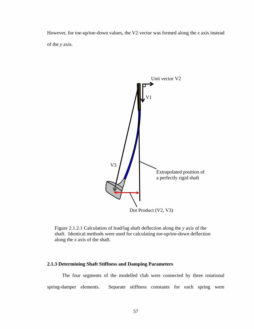
However, for toe-up/toe-down values, the V2 vector was formed along the x axis instead

of the y axis.

Unit vector V2

V1

V3

Dot Product (V2, V3)

Extrapolated position of a perfectly rigid shaft

Figure 2.1.2.1 Calculation of lead/lag shaft deflection along the y axis of the shaft. Identical methods were used for calculating toe-up/toe-down deflection along the x axis of the shaft.

2.1.3 Determining Shaft Stiffness and Damping Parameters

The four segments of the modelled club were connected by three rotational

spring-damper elements. Separate stiffness constants for each spring were

57

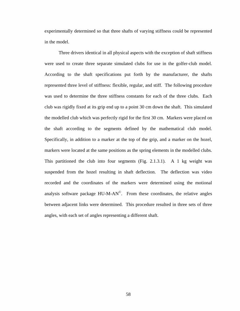
experimentally determined so that three shafts of varying stiffness could be represented

in the model.

Three drivers identical in all physical aspects with the exception of shaft stiffness

were used to create three separate simulated clubs for use in the golfer-club model.

According to the shaft specifications put forth by the manufacturer, the shafts

represented three level of stiffness: flexible, regular, and stiff. The following procedure

was used to determine the three stiffness constants for each of the three clubs. Each

club was rigidly fixed at its grip end up to a point 30 cm down the shaft. This simulated

the modelled club which was perfectly rigid for the first 30 cm. Markers were placed on

the shaft according to the segments defined by the mathematical club model.

Specifically, in addition to a marker at the top of the grip, and a marker on the hozel,

markers were located at the same positions as the spring elements in the modelled clubs.

This partitioned the club into four segments (Fig. 2.1.3.1). A 1 kg weight was

suspended from the hozel resulting in shaft deflection. The deflection was video

recorded and the coordinates of the markers were determined using the motional

analysis software package HU-M-AN©. From these coordinates, the relative angles

between adjacent links were determined. This procedure resulted in three sets of three

angles, with each set of angles representing a different shaft.

58

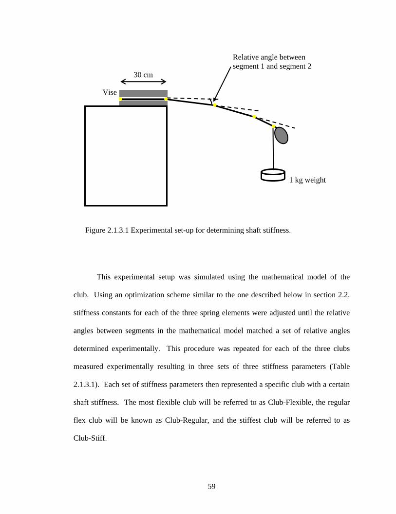
This experimental setup was simulated using the mathematical model of the

club. Using an optimization scheme similar to the one described below in section 2.2,

stiffness constants for each of the three spring elements were adjusted until the relative

angles between segments in the mathematical model matched a set of relative angles

determined experimentally. This procedure was repeated for each of the three clubs

measured experimentally resulting in three sets of three stiffness parameters (Table

2.1.3.1). Each set of stiffness parameters then represented a specific club with a certain

shaft stiffness. The most flexible club will be referred to as Club-Flexible, the regular

flex club will be known as Club-Regular, and the stiffest club will be referred to as

Club-Stiff.

Relative angle between segment 1 and segment 2

30 cm

Vise

1 kg weight

Figure 2.1.3.1 Experimental set-up for determining shaft stiffness.

59

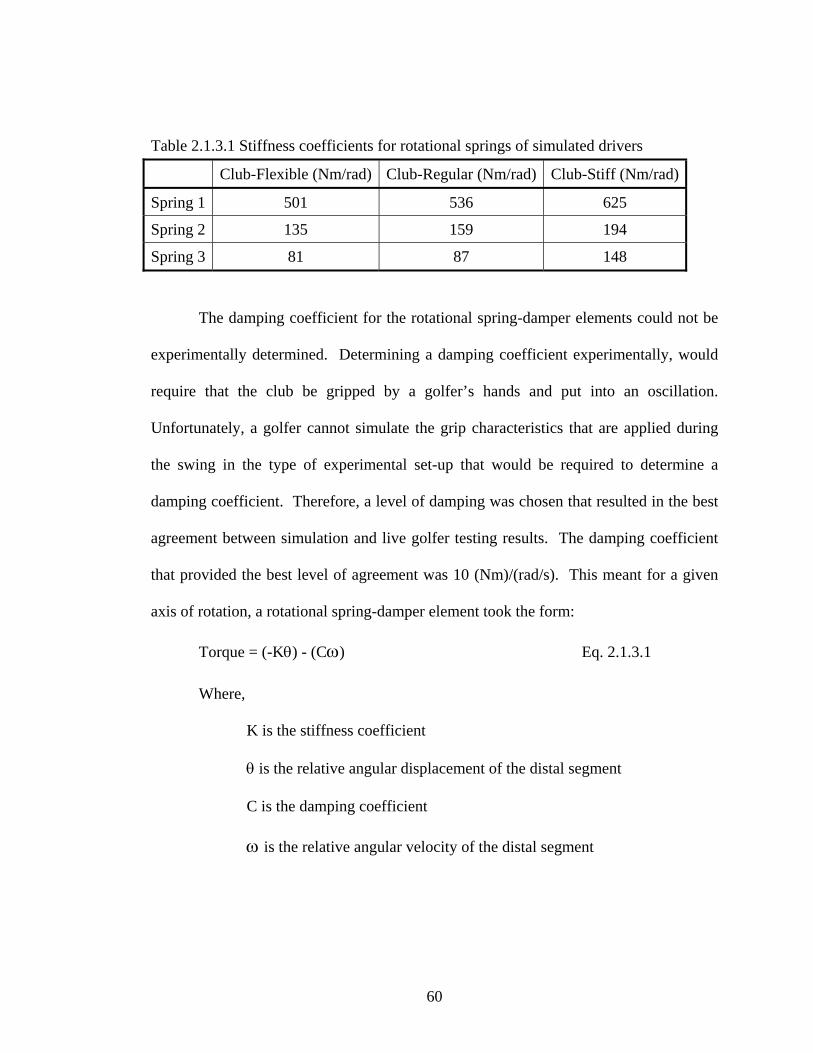
Table 2.1.3.1 Stiffness coefficients for rotational springs of simulated drivers

Club-Flexible (Nm/rad) Club-Regular (Nm/rad) Club-Stiff (Nm/rad)

Spring 1 501 536 625

Spring 2 135 159 194

Spring 3 81 87 148

The damping coefficient for the rotational spring-damper elements could not be

experimentally determined. Determining a damping coefficient experimentally, would

require that the club be gripped by a golfer’s hands and put into an oscillation.

Unfortunately, a golfer cannot simulate the grip characteristics that are applied during

the swing in the type of experimental set-up that would be required to determine a

damping coefficient. Therefore, a level of damping was chosen that resulted in the best

agreement between simulation and live golfer testing results. The damping coefficient

that provided the best level of agreement was 10 (Nm)/(rad/s). This meant for a given

axis of rotation, a rotational spring-damper element took the form:

Torque = (-Kθ) - (Cω) Eq. 2.1.3.1

Where,

K is the stiffness coefficient

θ is the relative angular displacement of the distal segment

C is the damping coefficient

ω is the relative angular velocity of the distal segment

60

2.1.4 Equations of Motion

The equations governing the motion of the mathematical model were based on

Newton’s Laws of Motion and were formulated according to Kane’s method

(Yamaguchi, 2001). The software program Autolev© was used to facilitate the

generation of the 3D dynamical equations into FORTRAN© programming code. To

solve the set of first order differential equations determining the motion of the system,

numerical integration was performed using a modified Kutta-Merson algorithm

provided by Autolev©. The Autolev© code is provided in Appendix C.

2.1.5 Generalized Coordinates of the Golfer Model

The following section was included to supply the reader with information that

would facilitate replication of the mathematical model used in this thesis. This

information is intended to be used in conjunction with the Autolev© code provided in

Appendix C. Knowledge of the following material is not necessary for comprehending

the results presented in this thesis; rather it simply offers a connection to the Autolev©

code. For those not familiar with Autolev©, proceed to section 2.2.

61

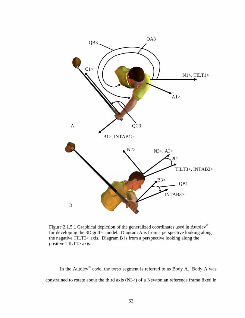
In the Autolev© code, the torso segment is referred to as Body A. Body A was

constrained to rotate about the third axis (N3>) of a Newtonian reference frame fixed in

QA3 QB3

N3>, A3>

TILT3>, INTAB3>

INTAB3>

QB1

20°

B3>

N2>

N1>, TILT1>

QC3

C1>

A1>

A

B1>, INTAB1>

B

Figure 2.1.5.1 Graphical depiction of the generalized coordinates used in Autolev© for developing the 3D golfer model. Diagram A is from a perspective looking along the negative TILT3> axis. Diagram B is from a perspective looking along the positive TILT1> axis.

62

the Autolev© environment. The angular position of the torso was defined by the angle

QA3. In order to have the arm segment move in a plane that was 20° steeper than the

torso plane, two reference frames (TILT, INTAB) were introduced. The TILT frame

was rotated 20° about N1> as shown in Figure 2.1.5.1B and was constrained to maintain

this orientation relative to N during all simulations. The INTAB reference frame was

constrained to rotate about the TILT3> axis. The arm segment, Body B, was attached to

INTAB, and therefore also rotated about TILT3>. The angular position of the arm, in

terms of horizontal abduction, was defined by the angle QB3 as shown in Figure

2.1.5.1A. To allow the arm segment to rotate about its longitudinal axis, Body B was

permitted to rotate about INTAB1>. The angular position of the arm, in terms of

external rotation about its longitudinal axis, was defined by the angle QB1 as shown in

Figure 2.1.5.1B. The most proximal segment of the club (which includes the hand),

Body C, was constrained to rotate about the third axis of the arm segment (B3>). The

angular position of the most proximal club segment was defined by the angle QC3 as

shown in Figure 2.1.5.1A. The reader is referred to Appendix C for the equations

relating the velocities of the various points on the model to the generalized coordinates.

2.2 Optimization of the Golfer-Club Model

Two separate sets of optimization schemes were conducted to fully explore the

concept of determining a precise shaft stiffness for a particular swing. The first scheme

involved manipulating the swing of the model to suit a particular level of shaft stiffness.

The second scheme manipulated the stiffness of the shaft to suit a particular model’s

63

swing. For both schemes, the objective in optimizing the golfer-club model was to

maximize horizontal clubhead speed at impact with the golf ball.

2.2.1 Customizing the Golfer to Fit the Club

The objective in customizing the golfer model to fit the club was to maximize

horizontal clubhead speed at impact with the golf ball. The objective function was equal

to horizontal clubhead speed at impact minus any penalty variables accumulated during

the simulated golf swing. Penalties were incurred if the model performed movements

that were not executable by a human golfer, such as having the arm segment pass

through the torso segment. Penalties were also incurred if the model was not in a proper

position at impact, such as having the clubface misaligned with the target. The

optimization scheme employed a single activation muscle control strategy where the

onset of voluntary torque at each joint was controlled separately. The control variables

were the onset and duration times for the four torque generators. This resulted in a total

of eight control variables that were optimized to determine maximum horizontal

clubhead speed at impact.

The optimization search engine was developed by myself and employed an

evolutionary algorithm approach as generally expressed by Michalewicz (1996). The

method was based on Darwin’s theories of evolution and natural selection in which the

fit individuals survive and pass on their genetic code to the next generation. In the case

of the golfer-club model, fitness was measured using the objective function (clubhead

speed minus penalties) and an individual was represented by a set of specific values for

the eight control variables. At the start of the optimization procedure, a population of

64

individuals was randomly generated and their fitness was evaluated. The higher an

individual’s fitness relative to the population, the greater the chance that individual had

in passing their genetic code (control variables) on to the next generation. All offspring

underwent a mutation in which one or more of their control variables were modified by

a random amount within a certain range of values. The range of values decreased as the

generation number increased so as to facilitate narrowing in on a maximum. In addition

to passing on their genetic code for mutation, the individual with the greatest relative

fitness persisted unaltered into the next generation. The programming language

Matlab© was used to create the optimization algorithm (Appendix D), which

communicated with the golfer-club model, developed in FORTRAN© (Appendix E). To

evaluate each individual, values for the eight control variables were sent to the golfer-

club model. The objective function was evaluated in FORTRAN© (a simulated swing

was executed) and the value (clubhead speed minus penalties) was returned to the

optimization algorithm where it represented an individual’s fitness in the population.

The optimization process maintained a population of 200 individuals that continually

evolved over 2000 generations. The fittest individual after the 2000th generation

represented the optimal set of control variables (muscle start and stop times) for the

particular model that was being optimized. Pilot work confirmed that population and

generation values of 200 and 2000 consistently returned the same set of control

variables. This process was repeated for each of the three golfer-club models

incorporating each level of shaft stiffness. It was previously stated that three models

were developed, each with a different ability to generate torque. This resulted in 9

65

optimized simulations. Essentially, the process resulted in 9 separate golfer models that

were each perfectly fitted to one of three clubs.

2.2.2 Customizing the Club to Fit the Golfer

In the previous section, methods were used to fine tune the swing of a golfer to

suit a particular shaft. The purpose of this section was to fine tune shaft stiffness to suit

a particular swing. It was possible that none of the three simulated clubs used in the

previous section were particularly suited to any of the three golfer models. A larger and

more complete spectrum of shaft stiffness was investigated in order to obtain a clearer

picture of the role that shaft stiffness plays in generating clubhead speed during the golf

swing.

The objective in customizing the stiffness of the shaft to the golfer model was

also to maximize horizontal clubhead speed at impact with the golf ball. A single

control variable, that regulated shaft stiffness, was used in the optimization scheme. The

control variable represented a percentage of the original stiffness of the rotational

spring-damper elements for Club-Regular. For example, Club-Regular had stiffness

coefficients of 536, 159, and 87 Nm/rad. Therefore, at the 50% stiffness level, the

stiffness coefficients were 268, 79.5, and 43.5 Nm/rad. An exhaustive search was

performed by evaluating all stiffness levels from 50 to 150% in 1% increments. This

range of stiffness was chosen to ensure that it encompassed the maximum range of

stiffness values that could be practically developed by manufacturers. For every

evaluation in the exhaustive search, the muscle control strategy used was that found for

66

the optimization of Golfer-Medium with Club-Regular in the previous section. This

procedure was also completed for Golfer-Slow and Golfer-Fast with Club-Regular.

2.3 Simulated Thought Experiments using the Golfer-Club Model

One of the big advantages of a mathematical model is that it permits

experimentation that would not be practical or in some cases not even possible in the

real world. Although it may have no direct application, information gained from

thought experiments can certainly help develop a deeper understanding of a

phenomenon. It is for this reason that additional simulations with the golfer-club model

were conducted.

2.3.1 Use of a Perfectly Rigid Shaft

It is not known to what extent a shaft can store and release energy in a useful

way during the golf swing. Even though it is not possible with live golfers, a

comparison of clubhead speeds attained with a flexible shaft versus a perfectly rigid

shaft would help answer the question. Once again, the three golfer models that only

differed in their ability to generate swing speed were employed. Each of the three golfer

models had the timing of their control torques optimized using the same method detailed

in section 2.2.1. However, for these optimizations, the golfer models were matched with

a perfectly rigid shaft. This shaft will be referred to as Club-Rigid. The shaft was

modelled as a single rigid link by incorporating motion constraints at the three joints that

connected the four club segments. The equations of motion used in the model were

reformulated in order to represent these constraints. Clubhead speeds attained by the

67

three rigid shaft models were compared to the clubhead speeds generated by their

respective non-rigid shaft models.

2.3.2 Repositioning the Clubhead Center of Mass

Several authors have stated that the shaft is deflected in the lead direction at

impact due to the radial force acting on the center of mass of the clubhead which is

offset from the axis of the shaft (Horwood, 1994; Jorgensen, 1994; Milne & Davis,

1992). The effect of the radial force will be to pull the center of mass of the clubhead

into a position that is collinear with the line of action of the radial force. If the radial

force is the dominating factor controlling shaft deflection at impact, then reversing the

position of the clubhead’s center of mass should reverse the direction of shaft bending.

If the center of mass is geometrically moved into a position in front of (positive y

direction) the longitudinal axis of the shaft (Fig. 1.2.1.1), then theoretically, the shaft

should be deflected in the lag direction at impact. This would be analogous to a left-

handed golfer swinging a right-handed driver. Similarly, if the center of mass of the

clubhead is positioned in-line with the shaft axis, then no deflection in the lead/lag

directions should be evident at impact with the ball.

The same theory holds for shaft deflection in the toe-up/toe-down direction. It

has been suggested that, at impact, the shaft is deflected in the toe-down direction due to

the action of radial force acting on the off-set center of mass of the clubhead (Horwood,

1994; Jorgensen, 1994; Milne & Davis, 1992). According to this theory, if the center of

mass is moved into a position below (negative x direction) the longitudinal axis of the

shaft (Fig. 1.2.1.1), then the shaft would be deflected in the toe-up direction at impact.

68

Likewise, if the center of mass was positioned in-line with the shaft axis, then the shaft

should be in a neutral toe-up/toe-down position at impact.

The above scenarios were tested using the optimized swing of Golfer-Medium

with Club-Regular. For each condition, the position of the center of mass of

Club_seg_4 (the most distal club segment) was only changed along either the x axis or

the y axis, and not both simultaneously. Shaft deflections were compared for three

positions of the center of mass along each axis: normal, in-line, and reversed. Normal

refers to the position of the center of mass in a typical driver. In-line refers to the center

of mass being collinear with the longitudinal axis of the shaft. Reversed refers to the

placement of the center of mass in the exact opposite location along a particular axis.

For example, normally the center of mass of Club_seg_4 is located 4.7 cm in the

negative y direction (Fig. 1.2.1.1 and Table 2.1.1.1). Therefore the reversed condition

would be to place the center of mass at 4.7 cm in the positive y direction. These tests

were conducted to gain a better understanding of the role of radial force in affecting

shaft deflection during the swing, and altering clubhead orientation at impact.

2.3.3 Removal and Isolation of Radial Force

Changing the position of the clubhead’s center of mass does help foster an

understanding of the influence of radial force on shaft bending. However, even if the

center of mass is geometrically placed in-line with the shaft, the shaft can still bend due

to tangential forces resulting in the clubhead center of mass no longer being collinear

and resulting in radial force once again exerting its influence.

69

Earlier, in section 1.2.5, I reasoned that resolving the forces applied to the club

by the golfer into tangential and radial components would help garner a better

understanding of shaft bending. I then described simple experiments that would

demonstrate the effects of these forces when acting in isolation. However, during the

golf swing, these forces never act in isolation and it would be a very difficult task to

tease out the specific effects of each force at any point in the swing. To gain a further

comprehension of the influence of radial force, shaft deflection could be compared

between a club swung in a normal fashion and a club swung in the absence of radial

force. In reality, it is not possible to swing a real golf club without applying a radial

force at the grip end, but it is possible to conduct such an experiment with a

mathematical model.

A simulation was conducted with the optimized Golfer-Medium\Club-Regular

combination. The force and torque values applied to the club during the swing were

recorded at each time step. The force and torque vectors were each broken down into

three components based on a reference frame fixed in the grip end of the club (Fig.

1.2.1.1). A second simulation was conducted with just the four segment Club-Regular

model in which the six force and torque measures taken at each time step in the previous

simulation served as input. As would be expected, the resulting clubhead speed and

shaft deflection measurements were identical to the first simulation in which Golfer-

Medium swung Club-Regular. A third simulation was performed in which the values

for the radial force at each time step were set to 0 N, but the other force and torque

measures remained the same. This allowed the effect of radial force to be removed from

the golf swing. A fourth simulation was performed in which only the values for radial

70

force were input at each time step, and all other force and torque measures were set

equal to zero. This allowed the effect of radial force to be isolated during the

downswing.

2.3.4 Effect of Shaft Deflection on Clubhead Orientation

Since the clubhead is rigidly fixed to the shaft, any amount of shaft deflection

will result in a change in clubhead orientation at impact and, therefore, ball flight

trajectory. With respect to the successful execution of a golf shot, shaft deflection can

alter the initial trajectory of the golf ball relative to two important planes. The first

plane is vertical and runs along the target line. Assuming a right-handed golfer, if shaft

deflection resulted in a closed clubface, then the initial ball trajectory will be to the left

of this vertical plane. If shaft deflection resulted in an open clubface, then the initial ball

trajectory will be to the right of the vertical plane. The second important plane is simply

represented by the horizontal surface of the ground. Relative to this plane, shaft

deflection can either result in a higher or lower ball flight trajectory. Of course, closing

the clubface, or adding more loft can also result from the position in which the golfer

orients the club at impact. To avoid ambiguity, any change in clubhead orientation at

impact relative to the two aforementioned planes that resulted entirely from shaft

deflection will be referred to as dynamic. For example, if shaft deflection results in an

additional two degrees of loft, then that two degrees will be referred to as dynamic loft.

Likewise, if shaft deflection results in the clubface being directed two degrees to the left

of the target line, then that two degrees will be referred to as dynamic close.

71

Shaft deflection about either the x or y axis (Fig. 1.2.1.1) alone will have an

effect on both dynamic loft and dynamic close. In other words, both dynamic loft and

dynamic close are a function of two variables, namely, lead deflection and toe-down

deflection. In order to quantify the effects that shaft deflection has on clubhead

orientation, two 3D plots were generated. One plotted dynamic loft versus toe-down

and lead deflections, while the second plotted dynamic close versus toe-down and lead

deflections. The range of lead and toe-down deflections used for graphing dynamic loft

and dynamic close were based on the maximum shaft deflection values attained during

the optimized swing of Golfer-Medium with Club-Regular.

2.4 Model Validation

2.4.1 External Validity

2.4.1.1 Live Golfer Testing

Four golfers with handicaps ranging from 3 to 30 were recruited to have their

swings filmed using high-speed video. Each golfer used three separate drivers; three

times each, from two perspectives for a total of 18 swings per golfer. From Perspective

1, participants were filmed with the camera perpendicular to the plane of the golf swing.

In order to orient the camera in a position that was approximately perpendicular to the

swing plane, the camera was placed 5.1 m away horizontally, and 5.5 m above ground

level (Fig. 2.4.1.1.1). From Perspective 2, the camera was positioned 4 m behind the

golfer pointing in the intended ball flight direction, such that at impact, the longitudinal

axis of the shaft would be perpendicular to the camera (Fig. 2.4.1.1.2). The three drivers

used during testing differed only in the flexibility of their shafts. These were the same

72

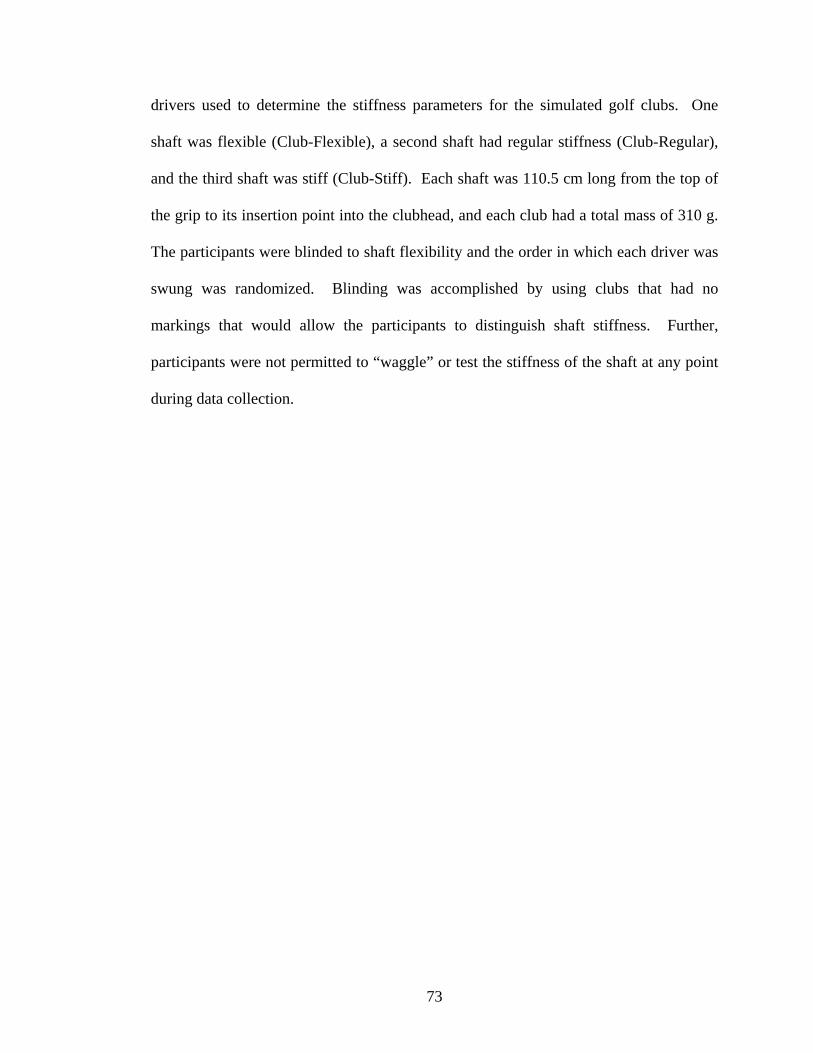
drivers used to determine the stiffness parameters for the simulated golf clubs. One

shaft was flexible (Club-Flexible), a second shaft had regular stiffness (Club-Regular),

and the third shaft was stiff (Club-Stiff). Each shaft was 110.5 cm long from the top of

the grip to its insertion point into the clubhead, and each club had a total mass of 310 g.

The participants were blinded to shaft flexibility and the order in which each driver was

swung was randomized. Blinding was accomplished by using clubs that had no

markings that would allow the participants to distinguish shaft stiffness. Further,

participants were not permitted to “waggle” or test the stiffness of the shaft at any point

during data collection.

73

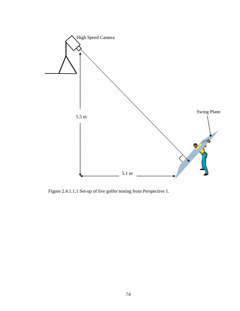
High Speed Camera

Swing Plane 5.5 m

5.1 m

Figure 2.4.1.1.1 Set-up of live golfer testing from Perspective 1.

74

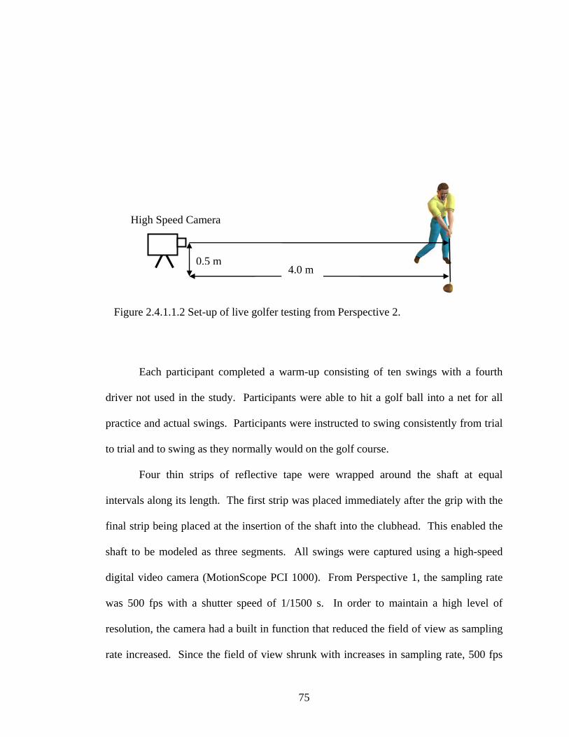
High Speed Camera

0.5 m4.0 m

Figure 2.4.1.1.2 Set-up of live golfer testing from Perspective 2.

Each participant completed a warm-up consisting of ten swings with a fourth

driver not used in the study. Participants were able to hit a golf ball into a net for all

practice and actual swings. Participants were instructed to swing consistently from trial

to trial and to swing as they normally would on the golf course.

Four thin strips of reflective tape were wrapped around the shaft at equal

intervals along its length. The first strip was placed immediately after the grip with the

final strip being placed at the insertion of the shaft into the clubhead. This enabled the

shaft to be modeled as three segments. All swings were captured using a high-speed

digital video camera (MotionScope PCI 1000). From Perspective 1, the sampling rate

was 500 fps with a shutter speed of 1/1500 s. In order to maintain a high level of

resolution, the camera had a built in function that reduced the field of view as sampling

rate increased. Since the field of view shrunk with increases in sampling rate, 500 fps

75

was the maximum sampling rate that could be used without excluding sections of the

golf swing. Also, due to size constraints of the testing lab, it was not possible to move

the camera further away from the participants, so as to increase the field of view. From

Perspective 2, the sampling rate was 1000 fps with a shutter speed of 1/3000 s. Only

three of the four golfers participated in the filming from Perspective 2. Also, a fifth

golfer (left-handed), videoed from Perspective 1, completed three swings with Club-

Regular while swinging left-handed.

Each swing was analyzed using the motion analysis software HU-M-AN©.

Displacement data throughout the swing for each strip of reflective tape was generated

by manually digitizing the center of each strip in each frame. The raw coordinate data

were smoothed using HU-M-AN’s built-in 4th order recursive Butterworth filter. Cut-

off frequencies, ranging from 15 to 19 Hz, were individually selected for each of the X

and Y coordinate data sets for each marker based on their residual plots. The smoothed

displacement data were numerically differentiated to determine velocity data for each

marked point on the shaft.

Shaft deflection for the live golfer testing was calculated in the same manner

described in section 1.2.1 and demonstrated in Figure 1.2.1.2. However, there were two

differences. First, from Perspective 1, shaft bending was only measured within the

plane of the swing and without any distinction between lead/lag and toe-up/toe-down

deflections. However, for the first three fifths of the downswing, the in-plane shaft

bending is almost completely in the toe-up/toe-down direction. While during the final

tenth of the downswing, in-plane bending is primarily in the lead/lag direction. Due to

the club rotating through 90° about the longitudinal axis of the lead arm, shaft deflection

76

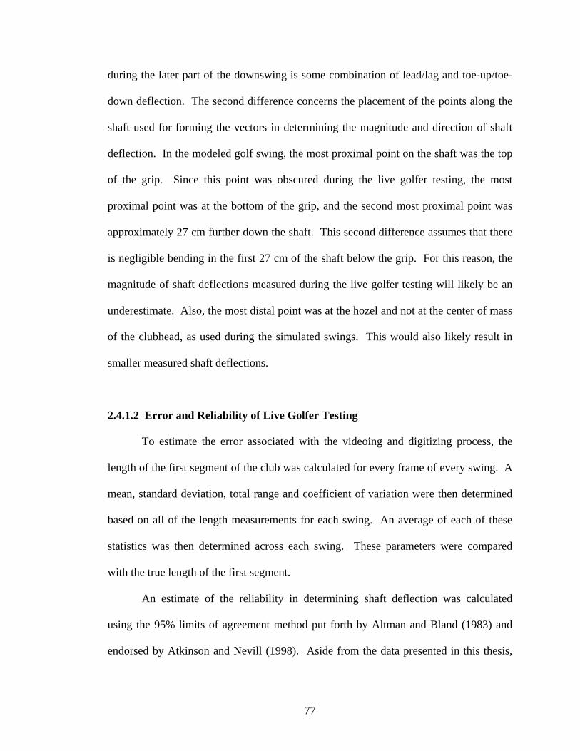
during the later part of the downswing is some combination of lead/lag and toe-up/toe-

down deflection. The second difference concerns the placement of the points along the

shaft used for forming the vectors in determining the magnitude and direction of shaft

deflection. In the modeled golf swing, the most proximal point on the shaft was the top

of the grip. Since this point was obscured during the live golfer testing, the most

proximal point was at the bottom of the grip, and the second most proximal point was

approximately 27 cm further down the shaft. This second difference assumes that there

is negligible bending in the first 27 cm of the shaft below the grip. For this reason, the

magnitude of shaft deflections measured during the live golfer testing will likely be an

underestimate. Also, the most distal point was at the hozel and not at the center of mass

of the clubhead, as used during the simulated swings. This would also likely result in

smaller measured shaft deflections.

2.4.1.2 Error and Reliability of Live Golfer Testing

To estimate the error associated with the videoing and digitizing process, the

length of the first segment of the club was calculated for every frame of every swing. A

mean, standard deviation, total range and coefficient of variation were then determined

based on all of the length measurements for each swing. An average of each of these

statistics was then determined across each swing. These parameters were compared

with the true length of the first segment.

An estimate of the reliability in determining shaft deflection was calculated

using the 95% limits of agreement method put forth by Altman and Bland (1983) and

endorsed by Atkinson and Nevill (1998). Aside from the data presented in this thesis,

77

each measure of shaft deflection was calculated on two other occasions. The standard

deviation of the difference scores between the two occasions was multiplied by 1.96 to

determine the 95% limits of agreement for a measurement of shaft deflection.

Essentially this means that if the same video data were analyzed twice, to determine

shaft deflection, then there would be a 95% chance that the difference between the two

deflection values would fall with-in the limits of agreement.

2.4.1.3 Swing Plane Comparison

Shaft bending aside, the ability of the model to move the club in a similar pattern

to actual golfers is an important validity concern. A good measure of comparison is the

swing plane. Currently, a mathematical model of golfer with varying swing plane does

not exist in the literature. The popular method of modeling the downswing as a 2D

motion was likely initially brought about by the necessity of a computationally simple

system due to the technology available at the time (Cochran & Stobbs, 1968; Jorgensen,

1970; Lampsa, 1975; Williams, 1967). Vaughn (1981), upon conducting a 3D

kinematic analysis of expert golfers, determined that the plane of the downswing varies

throughout the movement. This was more recently confirmed by Coleman and Rankin

(2005). A swing plane generated by the mathematical model used in this thesis was

compared to the swing plane measurements made by Coleman and Rankin in section

3.9.

78

2.4.2 Internal Validity

To ensure that the 3D equations of motion were correct and behaving in

accordance with Newton’s Laws of Motion a simple simulation was performed. The

potential and kinetic energies of the model’s six segments were calculated as they

rotated about a horizontal axis that passed through the middle of the torso segment. For

this simulation, no constraints were placed on the motion of the segments. Essentially,

the model behaved like a multi-segment pendulum solely under the influence of gravity.

If the sum of the potential and kinetic energies of the model remained constant during

the simulation, then it would be a strong indication that the equations of motion were

generated correctly. Also, an integration checking function provided by Autolev© was

implemented during each simulation to ensure that the integration was accurate to within

seven significant digits. Basically, the integration checking function determined if the

total force and torque inputs into the system balanced out with the resulting kinematics.

79

3

RESULTS

80

The format of the results section mirrors the sequence of experiments described

in the methods section. For each methods section there is a corresponding results

section with all pertinent findings that emerged from the experiments presented. Due to

the size of this document, it is recommended that a review of the corresponding method

section is made prior to reading each specific result section.

3.1 Optimization of the Golfer-Club Model

3.1.1 Typical Swing Results

The torque profiles for each of the 9 optimized simulations demonstrated the

same proximal to distal pattern of coordination (Fig. 3.1.1.1). The torso muscle torque

generator was always activated at t = 0, and was followed in sequence by the shoulder,

wrist, and arm rotation torques. Note that arm rotation refers to the external rotation of

the lead arm about its longitudinal axis during the downswing. For all simulations, the

torso, shoulder, and arm rotation torques remained active for the entire simulation. The

arm’s external rotation torque dropped to zero before the end of the simulation (Fig.

3.1.1.1). This occurred due to the force-velocity property imposed on the muscle torque

generator. As impact approached, the external rotation velocity of the arm segment was

too large for the muscle torque generator to apply an external rotation moment to the

segment.

81

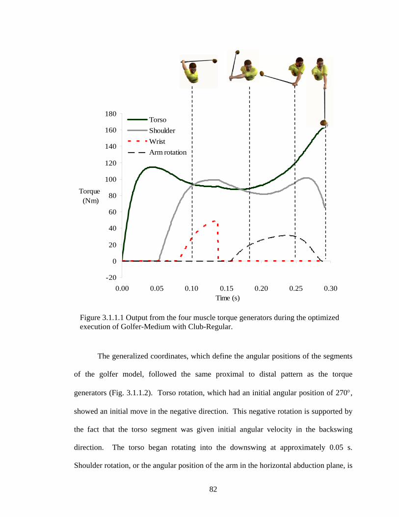
-20

0

20

40

60

80

100

120

140

160

180

0.00 0.05 0.10 0.15 0.20 0.25 0.30Time (s)

Torque (Nm)

TorsoShoulderWristArm rotation

Figure 3.1.1.1 Output from the four muscle torque generators during the optimized execution of Golfer-Medium with Club-Regular.

The generalized coordinates, which define the angular positions of the segments

of the golfer model, followed the same proximal to distal pattern as the torque

generators (Fig. 3.1.1.2). Torso rotation, which had an initial angular position of 270°,

showed an initial move in the negative direction. This negative rotation is supported by

the fact that the torso segment was given initial angular velocity in the backswing

direction. The torso began rotating into the downswing at approximately 0.05 s.

Shoulder rotation, or the angular position of the arm in the horizontal abduction plane, is

82

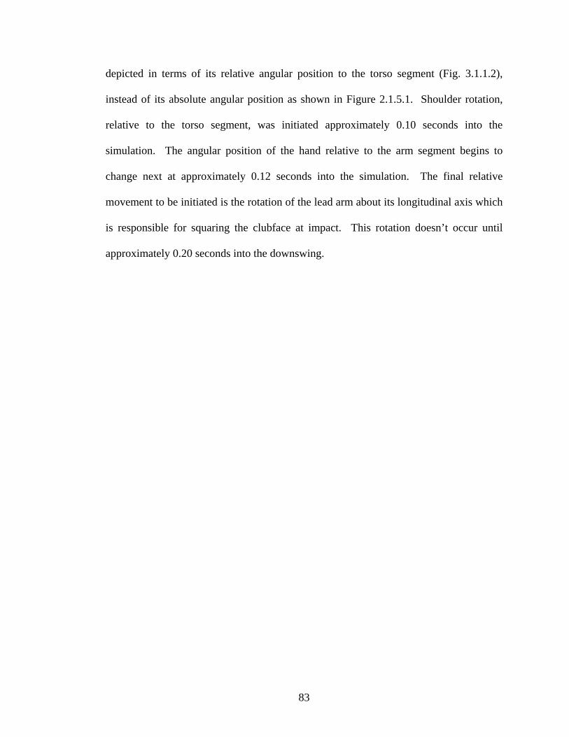
depicted in terms of its relative angular position to the torso segment (Fig. 3.1.1.2),

instead of its absolute angular position as shown in Figure 2.1.5.1. Shoulder rotation,

relative to the torso segment, was initiated approximately 0.10 seconds into the

simulation. The angular position of the hand relative to the arm segment begins to

change next at approximately 0.12 seconds into the simulation. The final relative

movement to be initiated is the rotation of the lead arm about its longitudinal axis which

is responsible for squaring the clubface at impact. This rotation doesn’t occur until

approximately 0.20 seconds into the downswing.

83

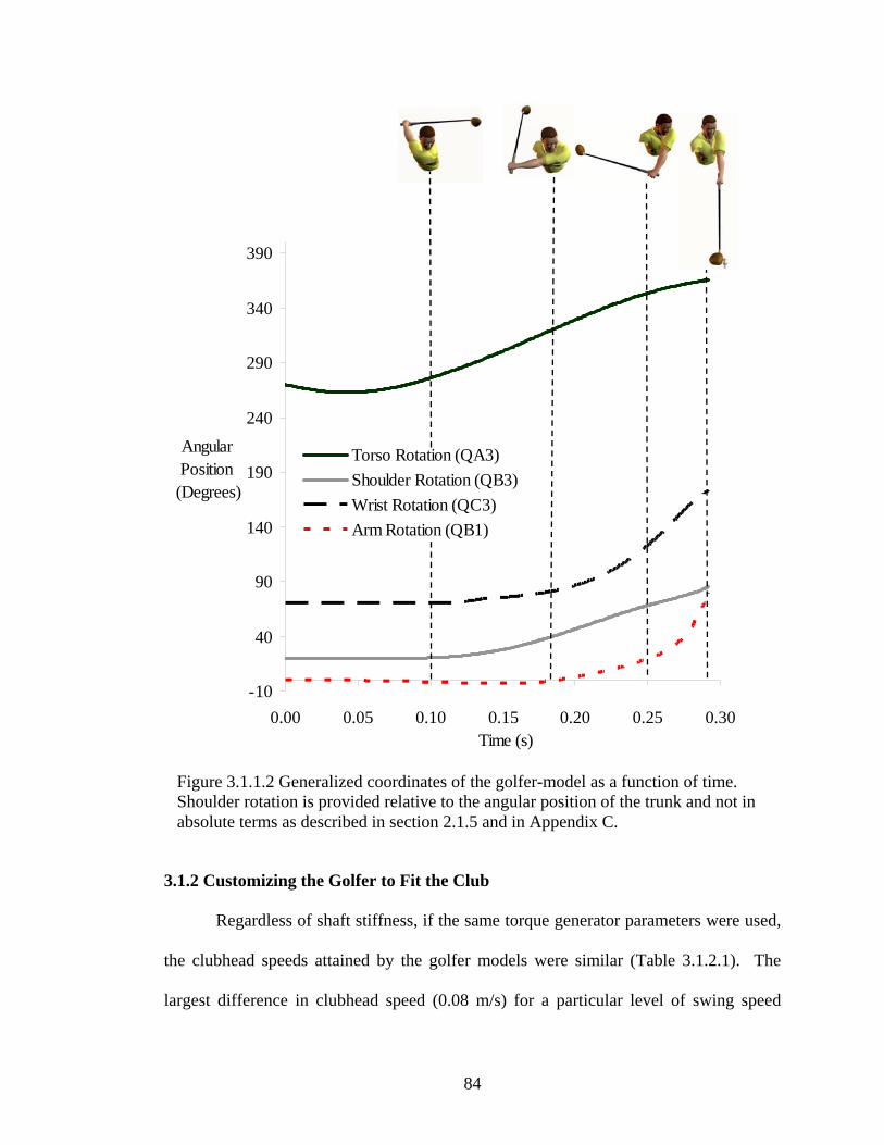
-10

40

90

140

190

240

290

340

390

0.00 0.05 0.10 0.15 0.20 0.25 0.30Time (s)

AngularPosition

(Degrees)

Torso Rotation (QA3)Shoulder Rotation (QB3)Wrist Rotation (QC3)Arm Rotation (QB1)

Figure 3.1.1.2 Generalized coordinates of the golfer-model as a function of time. Shoulder rotation is provided relative to the angular position of the trunk and not in absolute terms as described in section 2.1.5 and in Appendix C.

3.1.2 Customizing the Golfer to Fit the Club

Regardless of shaft stiffness, if the same torque generator parameters were used,

the clubhead speeds attained by the golfer models were similar (Table 3.1.2.1). The

largest difference in clubhead speed (0.08 m/s) for a particular level of swing speed

84

occurred with the Golfer-Medium model between Club-Stiff (45.04 m/s) and Club-

Flexible (44.96 m/s).

The constraints imposed on the optimization routine by the penalty variables

resulted in some imprecise relationships for the quantities presented in Table 3.1.2.1.

For example, a clear relationship did not exist for the ‘max toe-up’ measurement across

levels of shaft stiffness for the Golfer-Medium model (Table 3.1.2.1). The optimized

muscle coordination strategy that was determined for the Golfer-Medium/Club-Flexible

arrangement would have resulted in poor clubface alignment at impact for the Golfer-

Medium/Club-Regular pairing. Therefore, the optimization algorithm determined a

different optimal coordination strategy for that particular pairing which deflected the

shaft differently, but still resulted in a similar clubhead speed at impact. If identical

swings were used for each shaft, then specific mathematical relationships would have

become apparent, but this would have come at the expense of an optimized swing with a

correct impact position. This idea is explained more fully in the next section. The toe-

down deflections at impact also failed to demonstrate a clear relationship across

conditions. This was also related to the slight variations in muscle coordination

strategies between conditions.

Even with the confounding nature of the penalty variables, some clear

relationships amongst the shaft deflection measurements emerged across swing speed

and shaft stiffness conditions.

For every optimized swing, the maximum lead deflection of the shaft occurred

at impact. It was also apparent that lead deflection increased as shaft stiffness decreased

and that lead deflection decreased as swing speed decreased. For example, the largest

85

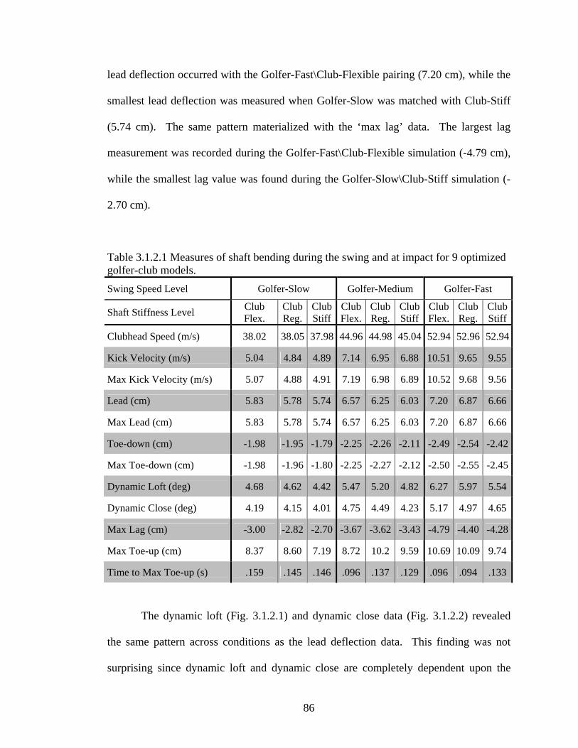
lead deflection occurred with the Golfer-Fast\Club-Flexible pairing (7.20 cm), while the

smallest lead deflection was measured when Golfer-Slow was matched with Club-Stiff

(5.74 cm). The same pattern materialized with the ‘max lag’ data. The largest lag

measurement was recorded during the Golfer-Fast\Club-Flexible simulation (-4.79 cm),

while the smallest lag value was found during the Golfer-Slow\Club-Stiff simulation (-

2.70 cm).

Table 3.1.2.1 Measures of shaft bending during the swing and at impact for 9 optimized golfer-club models. Swing Speed Level Golfer-Slow Golfer-Medium Golfer-Fast

Shaft Stiffness Level Club Flex.

ClubReg.

ClubStiff

ClubFlex.

ClubReg.

Club Stiff

Club Flex.

ClubReg.

ClubStiff

Clubhead Speed (m/s) 38.02 38.05 37.98 44.96 44.98 45.04 52.94 52.96 52.94

Kick Velocity (m/s) 5.04 4.84 4.89 7.14 6.95 6.88 10.51 9.65 9.55

Max Kick Velocity (m/s) 5.07 4.88 4.91 7.19 6.98 6.89 10.52 9.68 9.56

Lead (cm) 5.83 5.78 5.74 6.57 6.25 6.03 7.20 6.87 6.66

Max Lead (cm) 5.83 5.78 5.74 6.57 6.25 6.03 7.20 6.87 6.66

Toe-down (cm) -1.98 -1.95 -1.79 -2.25 -2.26 -2.11 -2.49 -2.54 -2.42

Max Toe-down (cm) -1.98 -1.96 -1.80 -2.25 -2.27 -2.12 -2.50 -2.55 -2.45

Dynamic Loft (deg) 4.68 4.62 4.42 5.47 5.20 4.82 6.27 5.97 5.54

Dynamic Close (deg) 4.19 4.15 4.01 4.75 4.49 4.23 5.17 4.97 4.65

Max Lag (cm) -3.00 -2.82 -2.70 -3.67 -3.62 -3.43 -4.79 -4.40 -4.28

Max Toe-up (cm) 8.37 8.60 7.19 8.72 10.2 9.59 10.69 10.09 9.74

Time to Max Toe-up (s) .159 .145 .146 .096 .137 .129 .096 .094 .133

The dynamic loft (Fig. 3.1.2.1) and dynamic close data (Fig. 3.1.2.2) revealed

the same pattern across conditions as the lead deflection data. This finding was not

surprising since dynamic loft and dynamic close are completely dependent upon the

86

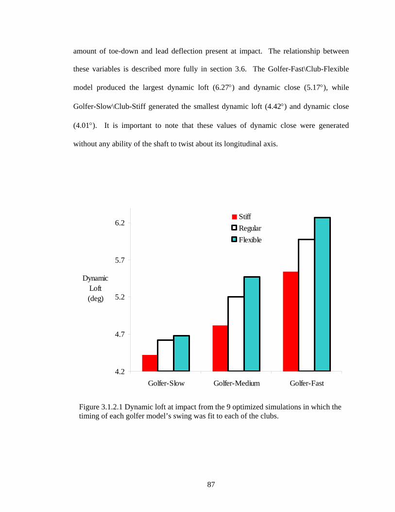
amount of toe-down and lead deflection present at impact. The relationship between

these variables is described more fully in section 3.6. The Golfer-Fast\Club-Flexible

model produced the largest dynamic loft (6.27°) and dynamic close (5.17°), while

Golfer-Slow\Club-Stiff generated the smallest dynamic loft (4.42°) and dynamic close

(4.01°). It is important to note that these values of dynamic close were generated

without any ability of the shaft to twist about its longitudinal axis.

4.2

4.7

5.2

5.7

6.2

Golfer-Slow Golfer-Medium Golfer-Fast

DynamicLoft(deg)

StiffRegularFlexible

Figure 3.1.2.1 Dynamic loft at impact from the 9 optimized simulations in which the timing of each golfer model’s swing was fit to each of the clubs.

87

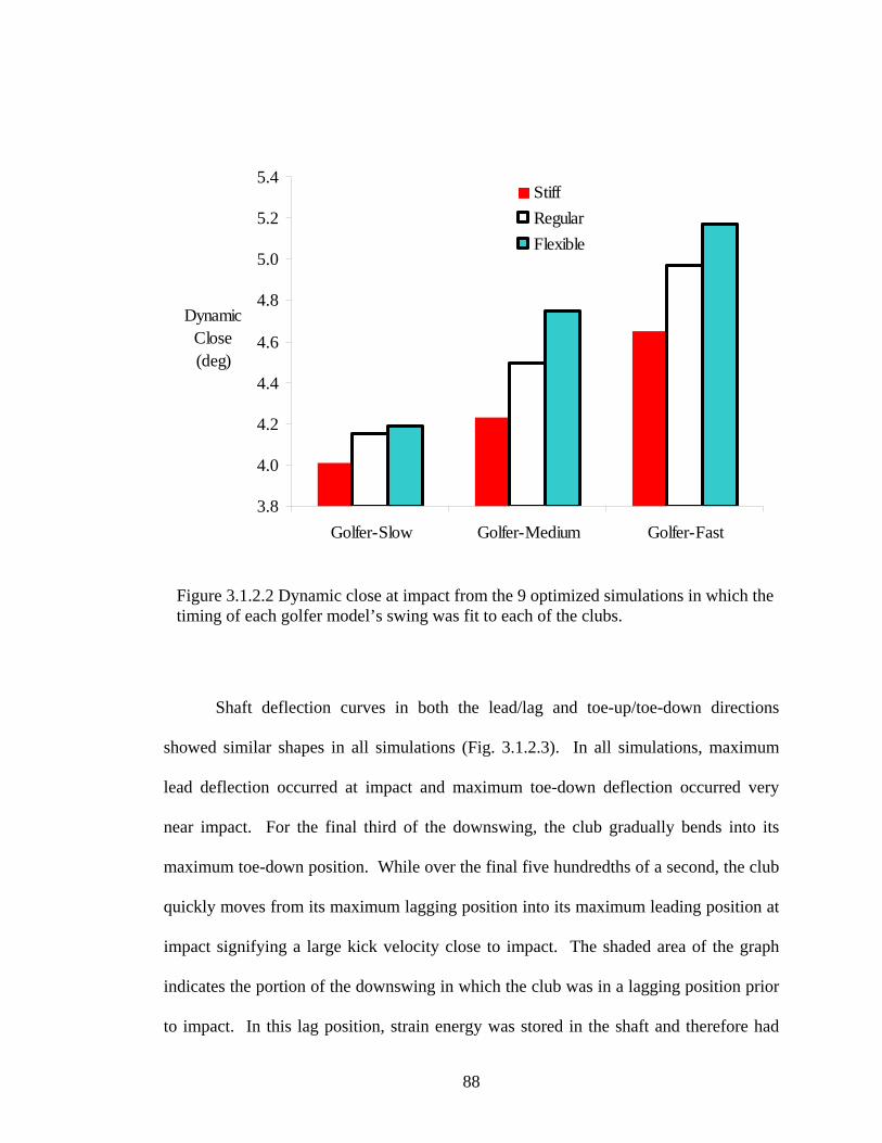
3.8

4.0

4.2

4.4

4.6

4.8

5.0

5.2

5.4

Golfer-Slow Golfer-Medium Golfer-Fast

DynamicClose(deg)

StiffRegularFlexible

Figure 3.1.2.2 Dynamic close at impact from the 9 optimized simulations in which the timing of each golfer model’s swing was fit to each of the clubs.

Shaft deflection curves in both the lead/lag and toe-up/toe-down directions

showed similar shapes in all simulations (Fig. 3.1.2.3). In all simulations, maximum

lead deflection occurred at impact and maximum toe-down deflection occurred very

near impact. For the final third of the downswing, the club gradually bends into its

maximum toe-down position. While over the final five hundredths of a second, the club

quickly moves from its maximum lagging position into its maximum leading position at

impact signifying a large kick velocity close to impact. The shaded area of the graph

indicates the portion of the downswing in which the club was in a lagging position prior

to impact. In this lag position, strain energy was stored in the shaft and therefore had

88

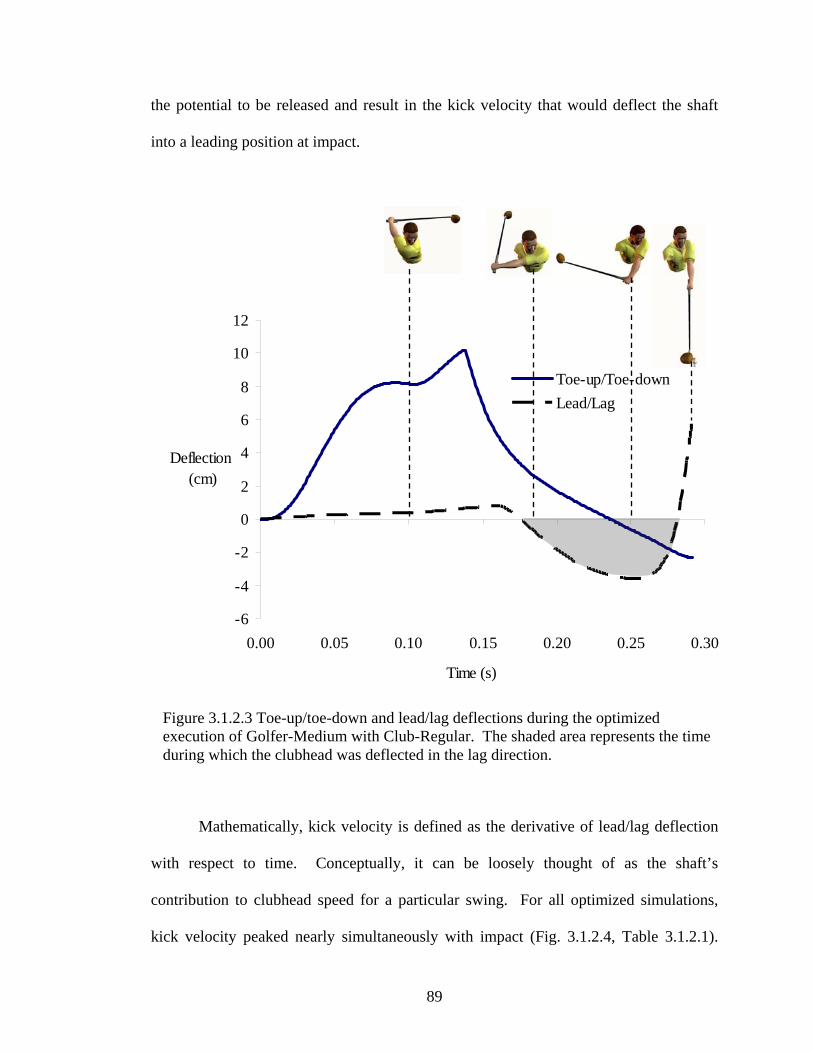
the potential to be released and result in the kick velocity that would deflect the shaft

into a leading position at impact.

Toe-down at impact

-6

-4

-2

0

2

4

6

8

10

12

0.00 0.05 0.10 0.15 0.20 0.25 0.30

Time (s)

Deflection (cm)

Toe-up/Toe-downLead/Lag

Figure 3.1.2.3 Toe-up/toe-down and lead/lag deflections during the optimized execution of Golfer-Medium with Club-Regular. The shaded area represents the time during which the clubhead was deflected in the lag direction.

Mathematically, kick velocity is defined as the derivative of lead/lag deflection

with respect to time. Conceptually, it can be loosely thought of as the shaft’s

contribution to clubhead speed for a particular swing. For all optimized simulations,

kick velocity peaked nearly simultaneously with impact (Fig. 3.1.2.4, Table 3.1.2.1).

89

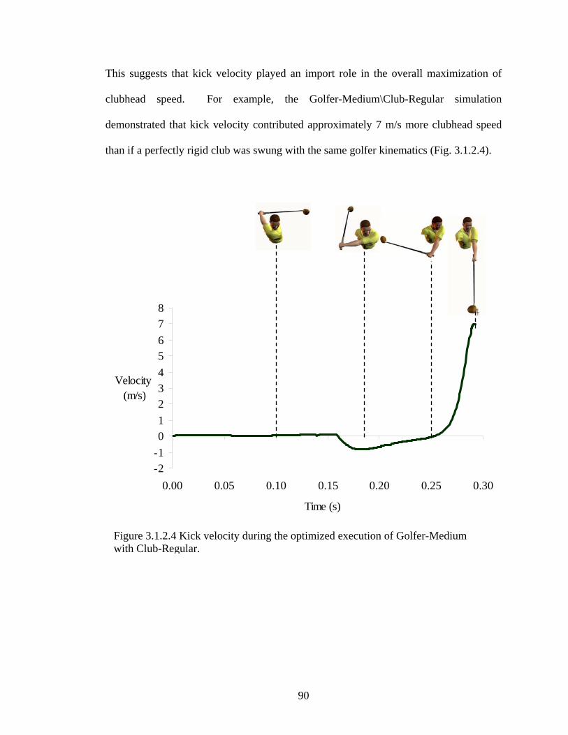
This suggests that kick velocity played an import role in the overall maximization of

clubhead speed. For example, the Golfer-Medium\Club-Regular simulation

demonstrated that kick velocity contributed approximately 7 m/s more clubhead speed

than if a perfectly rigid club was swung with the same golfer kinematics (Fig. 3.1.2.4).

-2-1012345678

0.00 0.05 0.10 0.15 0.20 0.25 0.30

Time (s)

Velocity (m/s)

Figure 3.1.2.4 Kick velocity during the optimized execution of Golfer-Medium with Club-Regular.

90

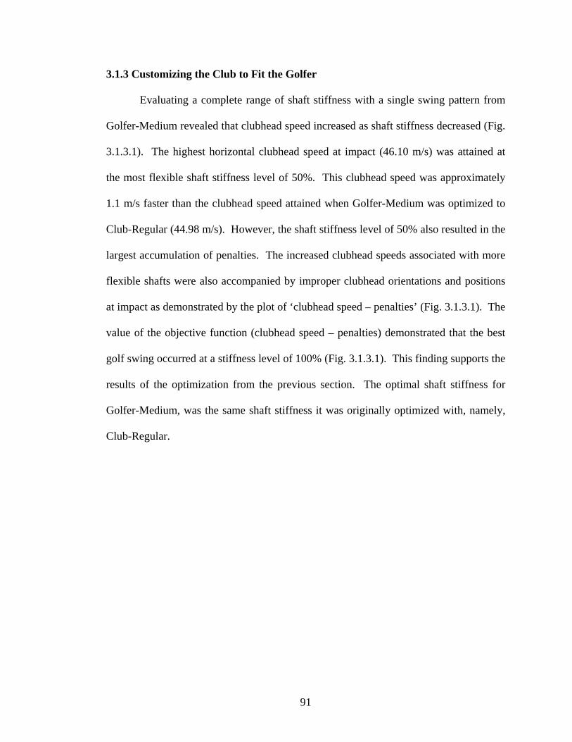
3.1.3 Customizing the Club to Fit the Golfer

Evaluating a complete range of shaft stiffness with a single swing pattern from

Golfer-Medium revealed that clubhead speed increased as shaft stiffness decreased (Fig.

3.1.3.1). The highest horizontal clubhead speed at impact (46.10 m/s) was attained at

the most flexible shaft stiffness level of 50%. This clubhead speed was approximately

1.1 m/s faster than the clubhead speed attained when Golfer-Medium was optimized to

Club-Regular (44.98 m/s). However, the shaft stiffness level of 50% also resulted in the

largest accumulation of penalties. The increased clubhead speeds associated with more

flexible shafts were also accompanied by improper clubhead orientations and positions

at impact as demonstrated by the plot of ‘clubhead speed – penalties’ (Fig. 3.1.3.1). The

value of the objective function (clubhead speed – penalties) demonstrated that the best

golf swing occurred at a stiffness level of 100% (Fig. 3.1.3.1). This finding supports the

results of the optimization from the previous section. The optimal shaft stiffness for

Golfer-Medium, was the same shaft stiffness it was originally optimized with, namely,

Club-Regular.

91

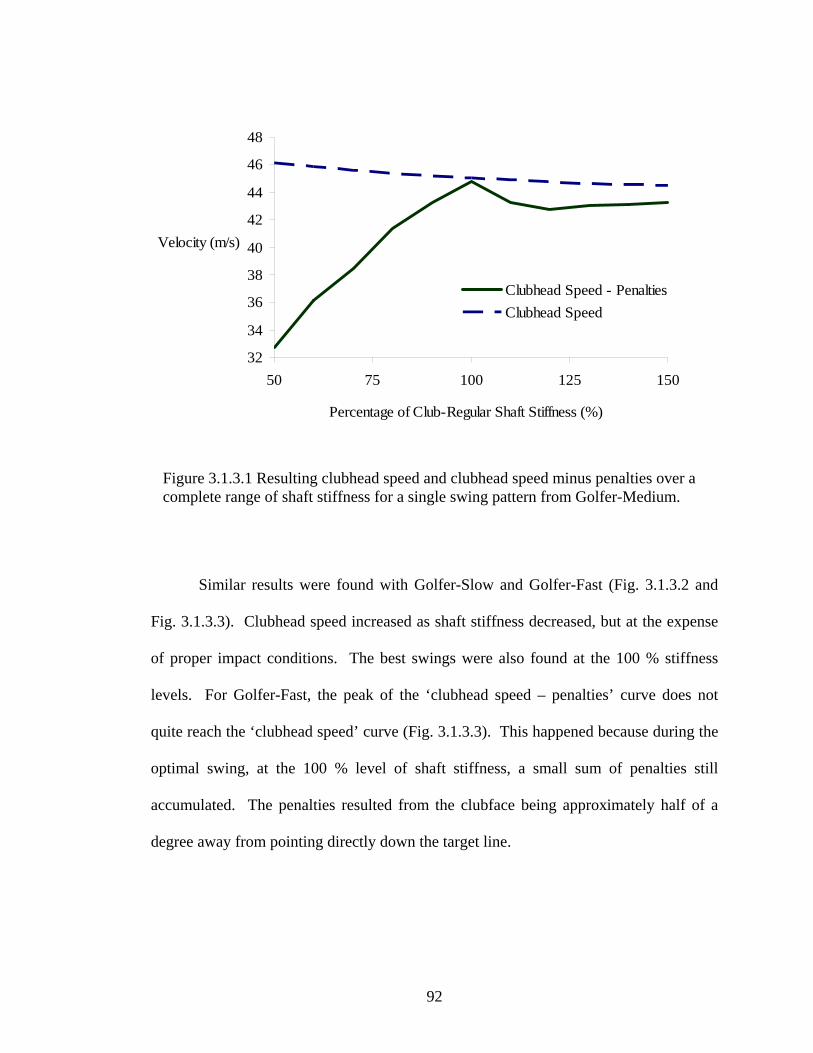
32

34

36

38

40

42

44

46

48

50 75 100 125 150

Percentage of Club-Regular Shaft Stiffness (%)

Velocity (m/s)

Clubhead Speed - PenaltiesClubhead Speed

Figure 3.1.3.1 Resulting clubhead speed and clubhead speed minus penalties over a complete range of shaft stiffness for a single swing pattern from Golfer-Medium.

Similar results were found with Golfer-Slow and Golfer-Fast (Fig. 3.1.3.2 and

Fig. 3.1.3.3). Clubhead speed increased as shaft stiffness decreased, but at the expense

of proper impact conditions. The best swings were also found at the 100 % stiffness

levels. For Golfer-Fast, the peak of the ‘clubhead speed – penalties’ curve does not

quite reach the ‘clubhead speed’ curve (Fig. 3.1.3.3). This happened because during the

optimal swing, at the 100 % level of shaft stiffness, a small sum of penalties still

accumulated. The penalties resulted from the clubface being approximately half of a

degree away from pointing directly down the target line.

92

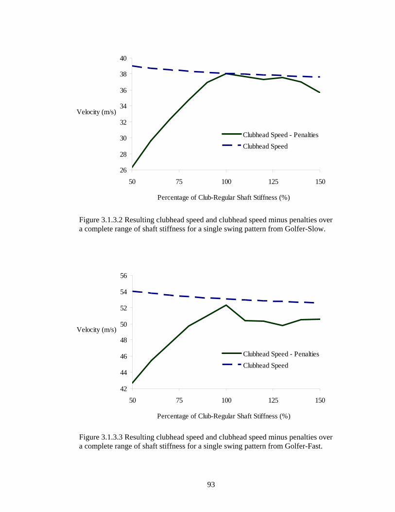
26

28

30

32

34

36

38

40

50 75 100 125 150

Percentage of Club-Regular Shaft Stiffness (%)

Velocity (m/s)

Clubhead Speed - PenaltiesClubhead Speed

Figure 3.1.3.2 Resulting clubhead speed and clubhead speed minus penalties over a complete range of shaft stiffness for a single swing pattern from Golfer-Slow.

42

44

46

48

50

52

54

56

50 75 100 125 150

Percentage of Club-Regular Shaft Stiffness (%)

Velocity (m/s)

Clubhead Speed - PenaltiesClubhead Speed

Figure 3.1.3.3 Resulting clubhead speed and clubhead speed minus penalties over a complete range of shaft stiffness for a single swing pattern from Golfer-Fast.

93

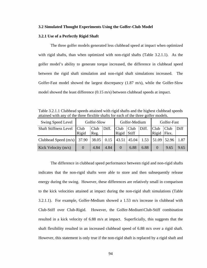
3.2 Simulated Thought Experiments Using the Golfer-Club Model

3.2.1 Use of a Perfectly Rigid Shaft

The three golfer models generated less clubhead speed at impact when optimized

with rigid shafts, than when optimized with non-rigid shafts (Table 3.2.1.1). As the

golfer model’s ability to generate torque increased, the difference in clubhead speed

between the rigid shaft simulation and non-rigid shaft simulations increased. The

Golfer-Fast model showed the largest discrepancy (1.87 m/s), while the Golfer-Slow

model showed the least difference (0.15 m/s) between clubhead speeds at impact.

Table 3.2.1.1 Clubhead speeds attained with rigid shafts and the highest clubhead speeds attained with any of the three flexible shafts for each of the three golfer models.

Swing Speed Level Golfer-Slow Golfer-Medium Golfer-Fast Shaft Stiffness Level Club

Rigid Club Reg.

Diff. Club Rigid

Club Stiff

Diff. Club Rigid

Club Flex.

Diff

Clubhead Speed (m/s) 37.90 38.05 0.15 43.51 45.04 1.53 51.09 52.96 1.87

Kick Velocity (m/s) 0 4.84 4.84 0 6.88 6.88 0 9.65 9.65

The difference in clubhead speed performance between rigid and non-rigid shafts

indicates that the non-rigid shafts were able to store and then subsequently release

energy during the swing. However, these differences are relatively small in comparison

to the kick velocities attained at impact during the non-rigid shaft simulations (Table

3.2.1.1). For example, Golfer-Medium showed a 1.53 m/s increase in clubhead with

Club-Stiff over Club-Rigid. However, the Golfer-Medium\Club-Stiff combination

resulted in a kick velocity of 6.88 m/s at impact. Superficially, this suggests that the

shaft flexibility resulted in an increased clubhead speed of 6.88 m/s over a rigid shaft.

However, this statement is only true if the non-rigid shaft is replaced by a rigid shaft and

94

no change in the kinematics of segments proximal to the rotational spring-damper

elements occurs. In reality, as well as in the model, the kinematics of the proximal

segments will change when the club is replaced. This is because the acceleration of the

system is not predetermined, but rather it is dictated by the forces and torques acting on

the segments. Since the two-segment golfer model dynamically interacts with the four-

segment club model, a rigid club will result in different golfer kinematics than a non-

rigid club. Taken together, these comments imply that, at impact, the angular velocity

of the most proximal club segment will be less with a non-rigid shaft as compared to a

rigid shaft. The angular velocities of the most proximal club segment, about an axis

perpendicular to the swing plane, for Golfer-Medium with Club-Stiff and Golfer-

Medium with Club-Rigid supported this view (Fig. 3.2.1.1).

95

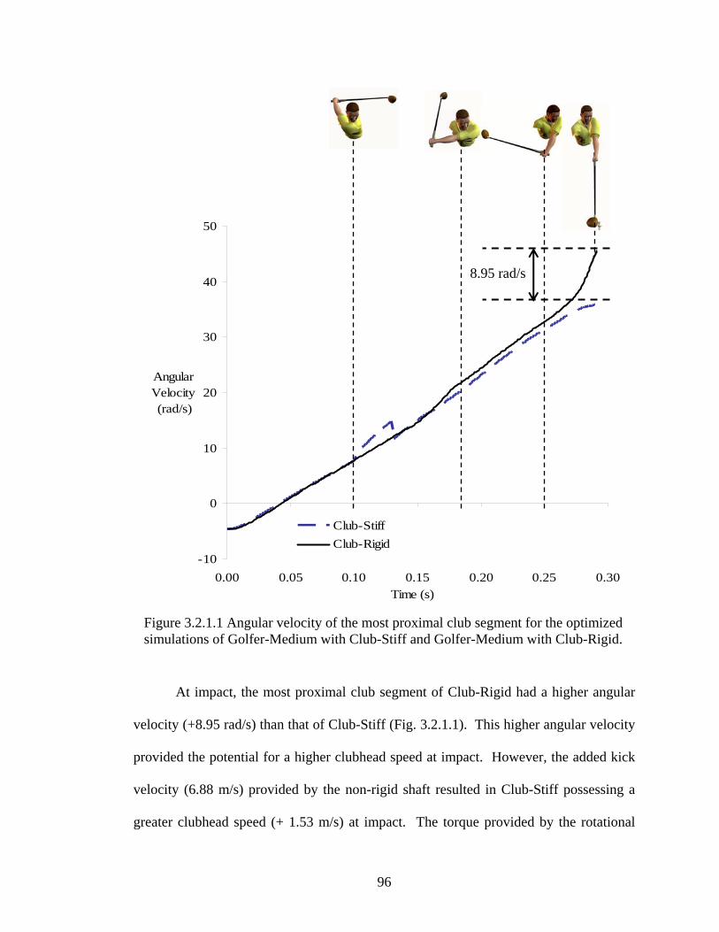
-10

0

10

20

30

40

50

0.00 0.05 0.10 0.15 0.20 0.25 0.30Time (s)

AngularVelocity (rad/s)

Club-StiffClub-Rigid

8.95 rad/s

Figure 3.2.1.1 Angular velocity of the most proximal club segment for the optimized simulations of Golfer-Medium with Club-Stiff and Golfer-Medium with Club-Rigid.

At impact, the most proximal club segment of Club-Rigid had a higher angular

velocity (+8.95 rad/s) than that of Club-Stiff (Fig. 3.2.1.1). This higher angular velocity

provided the potential for a higher clubhead speed at impact. However, the added kick

velocity (6.88 m/s) provided by the non-rigid shaft resulted in Club-Stiff possessing a

greater clubhead speed (+ 1.53 m/s) at impact. The torque provided by the rotational

96

spring-damper elements resulted in the added kick velocity. However, just as the torque

increases the clubhead velocity, it conversely decreases the angular velocity of the most

proximal club segment.

3.2.2 Repositioning the Clubhead Center of Mass

Repositioning the center of mass of the clubhead altered the behaviour of the

shaft by an amount large enough to have a meaningful effect on clubhead orientation at

impact. The effects of repositioning the center of mass along the two axes of shaft

deflection (x, y, see Fig. 1.2.1.1) were independent of one another. For example,

changing the position of the center of mass along the x axis only affected shaft

deflection in the toe-up/toe-down directions and had no measurable influence on

lead/lag deflection. Similarly, changing the position of the center of mass along the y

axis only affected shaft deflection in the lead/lag directions and had no measurable

influence on toe-up/toe-down deflection. For this reason toe-up/toe-down deflections

are presented separately in Figure 3.2.2.1 to demonstrate the effects of changing the

center of mass along the x axis. Lead/lag deflections are presented in Figure 3.2.2.2 to

demonstrate the effects of repositioning the center of mass along the y axis.

97

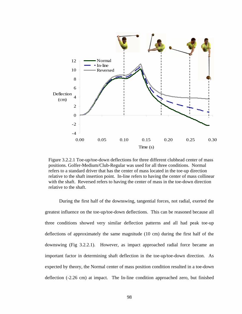
-4

-2

0

2

4

6

8

10

12

0.00 0.05 0.10 0.15 0.20 0.25 0.30

Time (s)

Deflection(cm)

Normal In-lineReversed

Figure 3.2.2.1 Toe-up/toe-down deflections for three different clubhead center of mass positions. Golfer-Medium/Club-Regular was used for all three conditions. Normal refers to a standard driver that has the center of mass located in the toe-up direction relative to the shaft insertion point. In-line refers to having the center of mass collinear with the shaft. Reversed refers to having the center of mass in the toe-down direction relative to the shaft.

During the first half of the downswing, tangential forces, not radial, exerted the

greatest influence on the toe-up/toe-down deflections. This can be reasoned because all

three conditions showed very similar deflection patterns and all had peak toe-up

deflections of approximately the same magnitude (10 cm) during the first half of the

downswing (Fig 3.2.2.1). However, as impact approached radial force became an

important factor in determining shaft deflection in the toe-up/toe-down direction. As

expected by theory, the Normal center of mass position condition resulted in a toe-down

deflection (-2.26 cm) at impact. The In-line condition approached zero, but finished

98

with a small toe-up deflection (0.69 cm) at impact. Reversing the center of mass

position along the x axis resulted in a relatively large toe-up deflection (3.60 cm) at

impact. If radial force completely dictated toe-down deflection at impact, then the In-

line condition would have resulted in a toe-up deflection of 0 cm at impact not 0.69 cm.

This toe-up deflection at impact for the In-line condition was a residual effect of the

large tangential forces that occurred earlier in the downswing. The same effect is also

evident in the other two conditions. For example, if 0.69 cm is subtracted from all three

conditions (-1.26, 0.69, +3.60), the result is a near symmetrical relationship around zero

(-2.95, 0, +2.91). This systematic shift suggests that the tangential forces applied earlier

in the downswing had a similar effect on all three conditions.

99

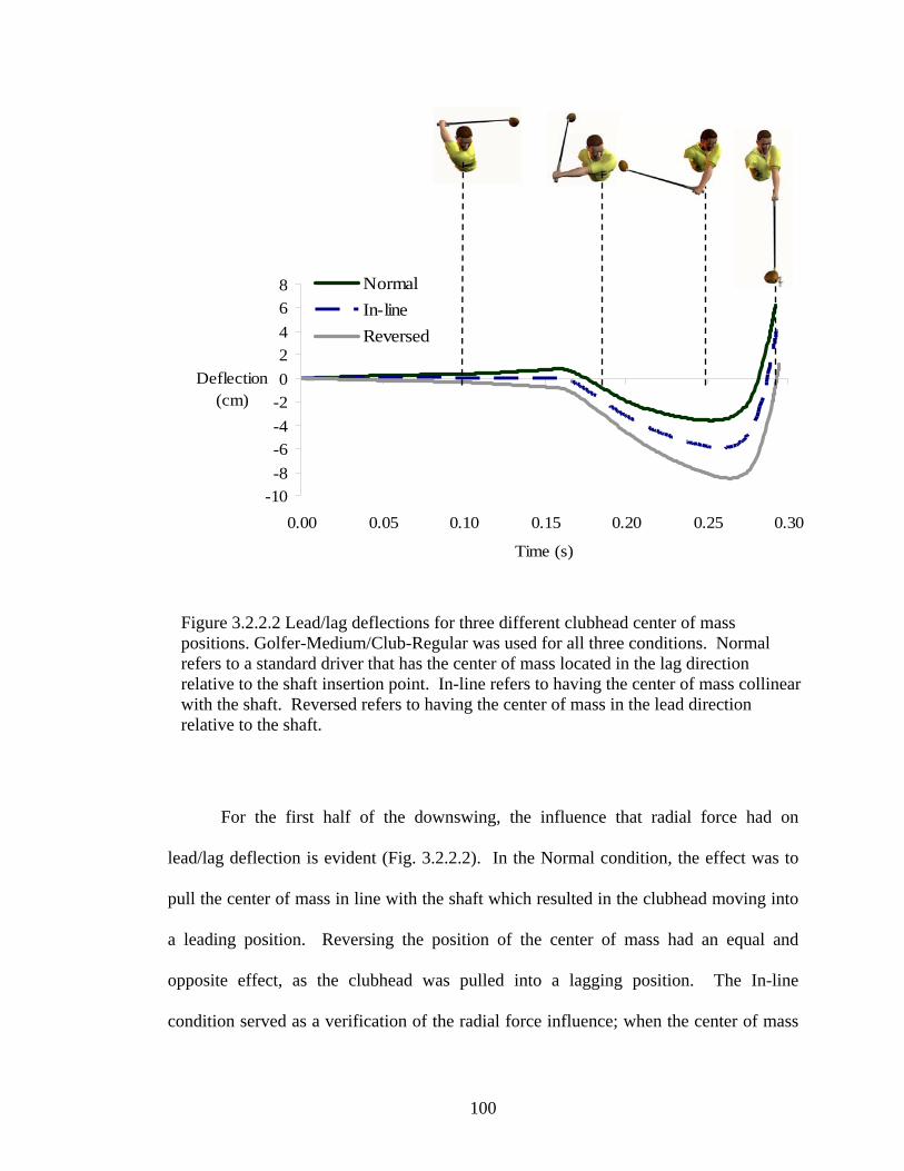
-10-8-6-4-202468

0.00 0.05 0.10 0.15 0.20 0.25 0.30

Time (s)

Deflection(cm)

NormalIn-lineReversed

Figure 3.2.2.2 Lead/lag deflections for three different clubhead center of mass positions. Golfer-Medium/Club-Regular was used for all three conditions. Normal refers to a standard driver that has the center of mass located in the lag direction relative to the shaft insertion point. In-line refers to having the center of mass collinear with the shaft. Reversed refers to having the center of mass in the lead direction relative to the shaft.

For the first half of the downswing, the influence that radial force had on

lead/lag deflection is evident (Fig. 3.2.2.2). In the Normal condition, the effect was to

pull the center of mass in line with the shaft which resulted in the clubhead moving into

a leading position. Reversing the position of the center of mass had an equal and

opposite effect, as the clubhead was pulled into a lagging position. The In-line

condition served as a verification of the radial force influence; when the center of mass

100

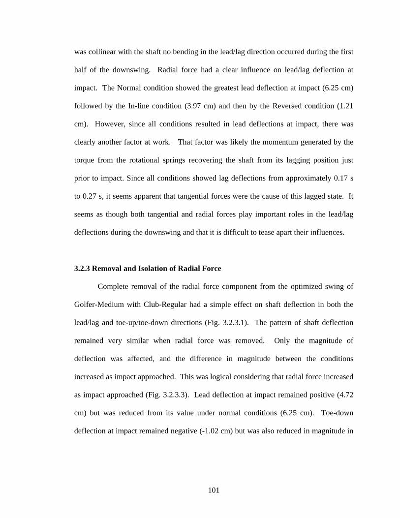
was collinear with the shaft no bending in the lead/lag direction occurred during the first

half of the downswing. Radial force had a clear influence on lead/lag deflection at

impact. The Normal condition showed the greatest lead deflection at impact (6.25 cm)

followed by the In-line condition (3.97 cm) and then by the Reversed condition (1.21

cm). However, since all conditions resulted in lead deflections at impact, there was

clearly another factor at work. That factor was likely the momentum generated by the

torque from the rotational springs recovering the shaft from its lagging position just

prior to impact. Since all conditions showed lag deflections from approximately 0.17 s

to 0.27 s, it seems apparent that tangential forces were the cause of this lagged state. It

seems as though both tangential and radial forces play important roles in the lead/lag

deflections during the downswing and that it is difficult to tease apart their influences.

3.2.3 Removal and Isolation of Radial Force

Complete removal of the radial force component from the optimized swing of

Golfer-Medium with Club-Regular had a simple effect on shaft deflection in both the

lead/lag and toe-up/toe-down directions (Fig. 3.2.3.1). The pattern of shaft deflection

remained very similar when radial force was removed. Only the magnitude of

deflection was affected, and the difference in magnitude between the conditions

increased as impact approached. This was logical considering that radial force increased

as impact approached (Fig. 3.2.3.3). Lead deflection at impact remained positive (4.72

cm) but was reduced from its value under normal conditions (6.25 cm). Toe-down

deflection at impact remained negative (-1.02 cm) but was also reduced in magnitude in

101

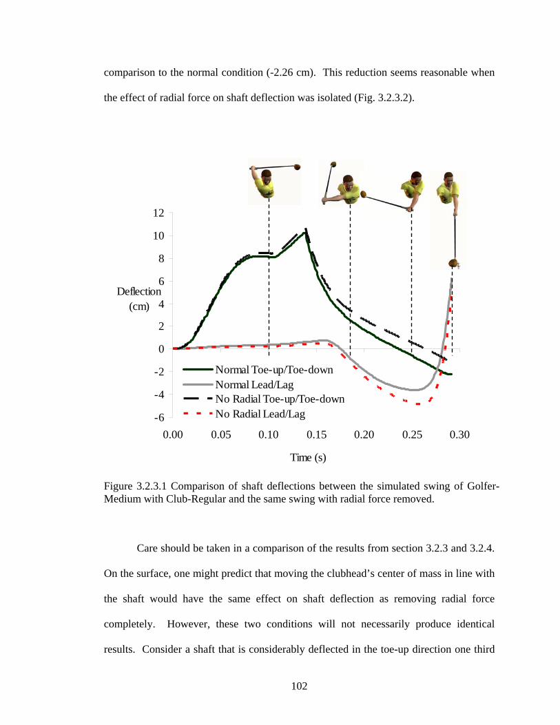
comparison to the normal condition (-2.26 cm). This reduction seems reasonable when

the effect of radial force on shaft deflection was isolated (Fig. 3.2.3.2).

-6

-4

-2

0

2

4

6

8

10

12

0.00 0.05 0.10 0.15 0.20 0.25 0.30

Time (s)

Deflection(cm)

Normal Toe-up/Toe-downNormal Lead/LagNo Radial Toe-up/Toe-downNo Radial Lead/Lag

Figure 3.2.3.1 Comparison of shaft deflections between the simulated swing of Golfer-Medium with Club-Regular and the same swing with radial force removed.

Care should be taken in a comparison of the results from section 3.2.3 and 3.2.4.

On the surface, one might predict that moving the clubhead’s center of mass in line with

the shaft would have the same effect on shaft deflection as removing radial force

completely. However, these two conditions will not necessarily produce identical

results. Consider a shaft that is considerably deflected in the toe-up direction one third

102

of the way into the downswing (Fig. 3.2.3.1). Even if the clubhead center of mass was

originally in the In-line position, radial force would still exert an influence because of

the clubhead’s current offset position. This influence would affect the dynamics of shaft

deflection for the rest of the swing. If radial force was removed completely, this would

not be the case.

When acting in isolation of all other forces and torques, radial force produced

nearly identical patterns of shaft deflections about both axes of shaft bending (Fig.

3.2.3.2). Due to the off-set position of the clubhead’s center of mass, the shaft was

gradually pulled into its maximum leading position (1.22 cm) at impact. Similarly, the

shaft was gradually pulled into its maximum toe-down position (-1.33 cm) at impact

when radial force acted as the lone contributor to shaft deflection. The club showed

more deflection in the toe-down direction than in the lead direction because the

clubhead center of mass was more off-set along the x axis (5.2 cm) than the y axis (4.7

cm) (Table 2.1.1.1).

103

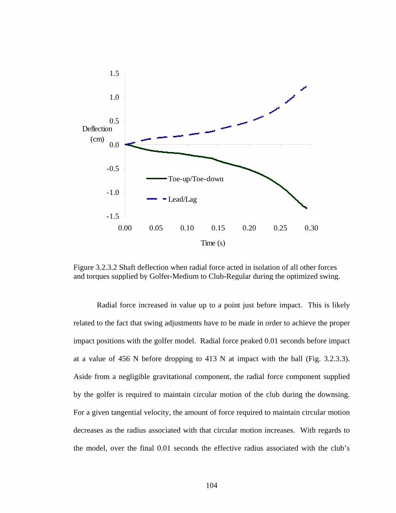
-1.5

-1.0

-0.5

0.0

0.5

1.0

1.5

0.00 0.05 0.10 0.15 0.20 0.25 0.30

Time (s)

Deflection(cm)

Toe-up/Toe-down

Lead/Lag

Figure 3.2.3.2 Shaft deflection when radial force acted in isolation of all other forces and torques supplied by Golfer-Medium to Club-Regular during the optimized swing.

Radial force increased in value up to a point just before impact. This is likely

related to the fact that swing adjustments have to be made in order to achieve the proper

impact positions with the golfer model. Radial force peaked 0.01 seconds before impact

at a value of 456 N before dropping to 413 N at impact with the ball (Fig. 3.2.3.3).

Aside from a negligible gravitational component, the radial force component supplied

by the golfer is required to maintain circular motion of the club during the downsing.

For a given tangential velocity, the amount of force required to maintain circular motion

decreases as the radius associated with that circular motion increases. With regards to

the model, over the final 0.01 seconds the effective radius associated with the club’s

104

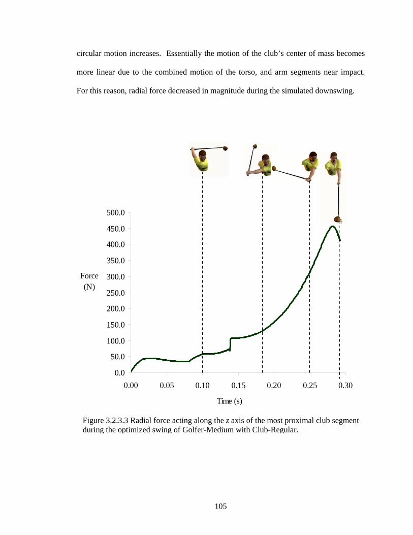
circular motion increases. Essentially the motion of the club’s center of mass becomes

more linear due to the combined motion of the torso, and arm segments near impact.

For this reason, radial force decreased in magnitude during the simulated downswing.

0.0

50.0

100.0

150.0

200.0

250.0

300.0

350.0

400.0

450.0

500.0

0.00 0.05 0.10 0.15 0.20 0.25 0.30

Time (s)

Force(N)

Figure 3.2.3.3 Radial force acting along the z axis of the most proximal club segment during the optimized swing of Golfer-Medium with Club-Regular.

105

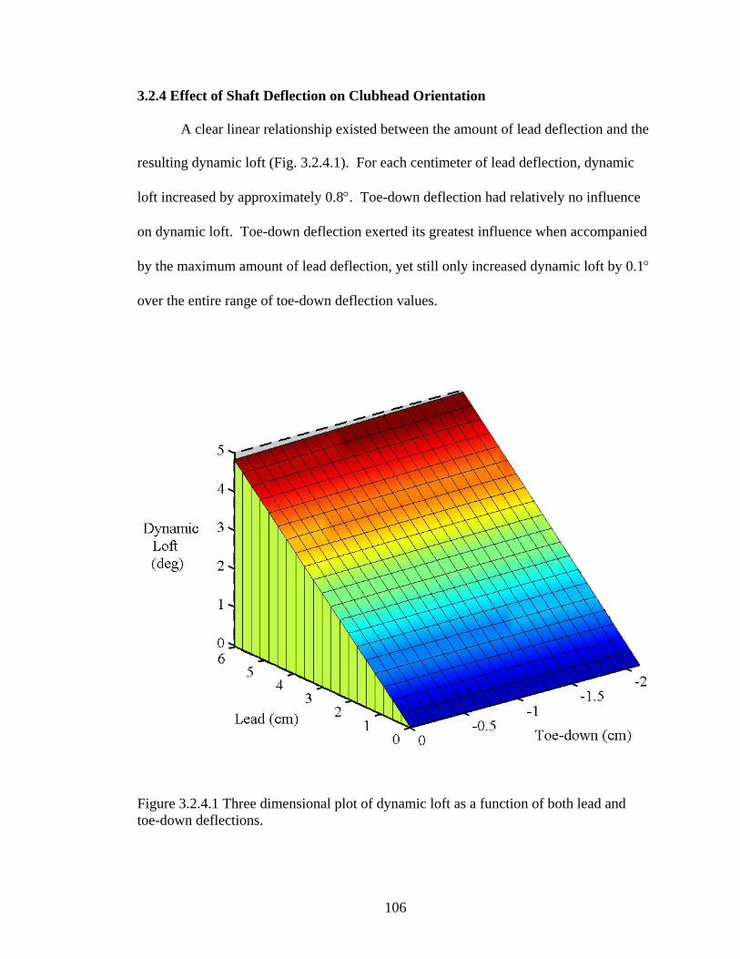
3.2.4 Effect of Shaft Deflection on Clubhead Orientation

A clear linear relationship existed between the amount of lead deflection and the

resulting dynamic loft (Fig. 3.2.4.1). For each centimeter of lead deflection, dynamic

loft increased by approximately 0.8°. Toe-down deflection had relatively no influence

on dynamic loft. Toe-down deflection exerted its greatest influence when accompanied

by the maximum amount of lead deflection, yet still only increased dynamic loft by 0.1°

over the entire range of toe-down deflection values.

Figure 3.2.4.1 Three dimensional plot of dynamic loft as a function of both lead and toe-down deflections.

106

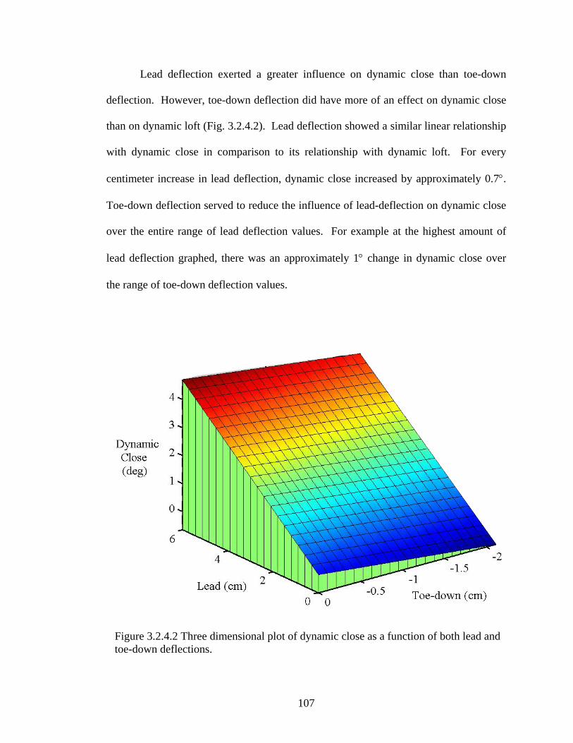
Lead deflection exerted a greater influence on dynamic close than toe-down

deflection. However, toe-down deflection did have more of an effect on dynamic close

than on dynamic loft (Fig. 3.2.4.2). Lead deflection showed a similar linear relationship

with dynamic close in comparison to its relationship with dynamic loft. For every

centimeter increase in lead deflection, dynamic close increased by approximately 0.7°.

Toe-down deflection served to reduce the influence of lead-deflection on dynamic close

over the entire range of lead deflection values. For example at the highest amount of

lead deflection graphed, there was an approximately 1° change in dynamic close over

the range of toe-down deflection values.

Figure 3.2.4.2 Three dimensional plot of dynamic close as a function of both lead and toe-down deflections.

107

3.3 Model Validation

3.3.1 External Validity

3.3.1.1 Live Golfer Testing

There was a trend for lead deflection at impact to increase in magnitude as shaft

stiffness decreased (Table 3.3.1.1.1). This finding supports the results for the lead

deflections measured during the simulations. For three out of the four live golfers

tested, Club-Flexible had the most lead deflection at impact followed by Club-Regular

and then by Club-Stiff. The other right-handed golfer, Live Golfer 3, produced the most

lead deflection with Club-Flexible, but Club-Stiff showed slightly more lead deflection

(0.76 ± 0.57 cm) than Club-Regular (0.44 ± 0.21 cm). Some inconsistency in the live

golfer testing results is to be expected. Williams and Sih (2002) reported an average

w

strong indication that lead deflection was also highly variable.

There appeared to be no relationship between lead deflection and clubhead speed

lfer testing. For example, Live Golfer 4, generated the slowest

ith Club-Flexible (39.13 ± 0.67 m/s), yet produced the greatest

± 0.10 cm) with the same club. Further, while swinging

0.21 cm) and highest (2.90 ± 0.61 cm) average lead deflections respectively with the

same club.

ithin subject standard deviation of 2.94° for loft angle with a single driver which is a

at impact for the live go

average clubhead speed w

average lead deflection (3.64

Club-Regular, both Live Golfer 3 and Live Golfer 4 had the same average clubhead

speeds at impact (39.63 ± 2.15 m/s, 39.63 ± 2.02 m/s), yet produced the lowest (0.44 ±

108

The lack of a relationship between clubhead speed and lead deflection appears

not to support the simulation data. However, the simulation data were derived from

optimized swings in which the club and golfer were perfectly matched to generate the

highest clubhead speed possible. Each optimized simulation also showed relatively

similar

nearly the same. Therefore, the resulting magnitudes of shaft deflection due to that

radial f

generation of clubhead speed, the majority of the shaft deflection during the first 75% of

the downswing, and at least half of the resulting deflections at impact. However, very

different patterns of tangential force can result in the same clubhead speed but with very

different patterns of shaft deflections during the swing and at impact. The live golfers

were probably employing relatively inconsistent and sub-optimal (compared to the

model) muscle coordination strategies. Therefore, it is likely that the live golfers, due to

differing muscle coordination strategies, generated different patterns of tangential

forces. These varying tangential force applications would be responsible for the lack of

a clubhead speed - shaft deflection relationship. Further, the clubhead speeds generated

from the computer simulation results ranged from 38 to 53 m/s, while the live golfers

patterns of muscle torque generation which were responsible for both the forces

applied to the club and the generation of clubhead speed. Shaft deflection is directly

influenced by the forces applied to the club, and not essentially by the velocity that

results from those forces (Butler & Winfield, 1994; Mather & Cooper, 1994). Radial

force is responsible for maintaining the circular motion of the club and approximately

half of the resulting deflections at impact. For a given clubhead speed at impact, the

amount of radial force required to maintain a particular curved motion will always be

orce will also be the same. The tangential forces are responsible for the

109

had a range of 37 to 43 m/s. This smaller range of clubhead speeds would also make it

difficult to detect differences in shaft deflection variables as a function of clubhead

speed.

While swinging the right-handed Club-Regular, lead deflections hovered around

zero (-0.11 ± 0.08 cm) for the left-handed golfer. It was likely that the reversed position

of the clubhead’s center of mass along the y axis resulted in the lack of lead deflection at

impact for the left-handed golfer despite a relatively high average clubhead speed (45.07

± 0.24 m/s). This finding is in agreement with the simulation results generated when the

clubhead center of mass position was reversed along the y axis for the Golfer-

Medium/Club-Regular pairing. This certainly suggests that radial force plays an

important in role in shaft deflection at impact. However it also implies, as did the

simulation results from section 3.2.2, that radial force does not completely dictate the

magnitude shaft deflection at impact. If radial force was completely dictating shaft

deflection at impact, then the shaft would be deflected by a larger amount in the lag

direction, and not just in a relatively neutral position (-0.11 ± 0.08 cm).

Two additional points should be made regarding the results from the Perspective

1 highspeed video data. First, with the exception of the left-handed golfer, every swing

with every club resulted in a lead deflection at impact, as did the simulation results.

This is a strong indication that the golfer model possesses a sufficient level of external

validity. Second, none of the golfers demonstrated consistently higher clubhead speeds

with any single club. Compared to the other participants, Live Golfer 3 had the largest

difference in average clubhead speed between the two clubs he performed the best with.

Live Golfer 3 had his highest average clubhead speed with Club-Flexible (41.7 ± 1.73

110

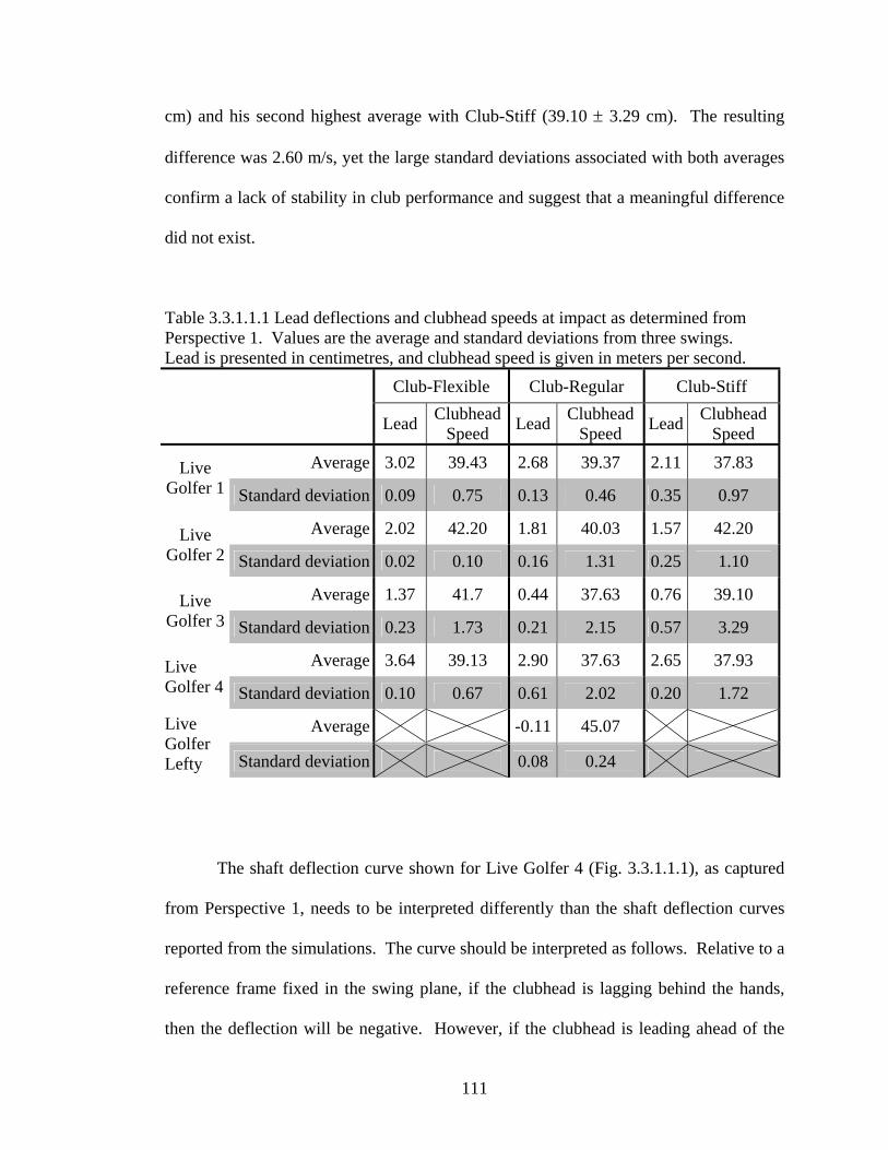
cm) and his second highest average with Club-Stiff (39.10 ± 3.29 cm). The resulting

difference was 2.60 m/s, yet the large standard deviations associated with both averages

confirm a lack of stability in club performance and suggest that a meaningful difference

did not exist.

Table 3.3.1.1.1 Lead deflections and clubhead speeds at impact as determined from

Lead is presented in centimetres, and clubhead speed is given in meters per second.

Club-Flexible Club-Regular Club-Stiff

Perspective 1. Values are the average and standard deviations from three swings.

Lead Speed Lead Speed Lead Speed Clubhead Clubhead Clubhead

Average 3.02 39.43 2.68 39.37 2.11 37.83 Live Golfer 1 Standard deviation 0.09 0.75 0.13 0.46 0.35 0.97

Average 2.02 42.20 1.81 40.03 1.57 42.20 Live Golfer 2 Standard deviation 0.02 0.10 0.16 1.31 0.25 1.10

Average 1.37 41.7 0.44 37.63 0.76 39.10 Live Golfer 3 Standard deviation 0.23 1.73 0.21 2.15 0.57 3.29

Average 3.64 39.13 2.90 37.63 2.65 37.93 Live Golfer 4 Standard deviation 0.10 0.67 0.61 2.02 0.20 1.72

Average -0.11 45.07 Live Golfer

ty Lef Standard deviation 0.08 0.24

The shaft deflection curve shown for Live Golfer 4 (Fig. 3.3.1.1.1), as captured

from eeds to b r t e s

re from the sim . urv d be interpreted as fo

sw lan he c ead ing nd t nds,

then the deflection will be negativ However, if the

Perspective 1, n e inte preted differently han the shaft defl ction curve

ported

reference

ulations The c e shoul llows. Relative to a

frame fixed in the ing p e, if t lubh is lagg behi he ha

e. the clubhead is leading ahead of

111

hands, then the deflection will sitiv ere the de n o haft

at art of the dow orde ega eca cl d w ing

e fixed in the swing plane. All golfers with all

bs demonstrated the same genera

swing. Tha pa ern was negative deflection for 80 - 90 % of the

in tive eflection over nal 0 %. Larger n gative

haft deflections were recorded as shaft stiffness decreased. These results are in

greement with the simulation results and indicate that the mathematical model was able

to suff

be po e. Th fore, toe-up flectio f the s

the st

the hands relative to a reference fram

nswing was rec d as n tive b use the ubhea as trail

three clu l pattern of shaft deflection during the

down

downsw

t general tt

g followed by posi d the fi 10 - 2 e

s

a

iciently represent the pattern of shaft bending during the downswing. The

magnitudes of shaft deflection measured during the live golfer testing were consistently

less during all points in the downswing. This was predictable and expected based on the

differences in the methods used to calculate shaft deflection in the live golfer versus

simulation experiments described in section 2.4.1.

112

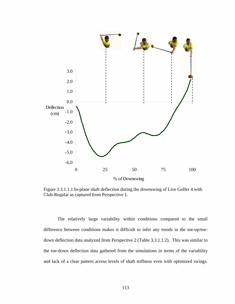
-6.0

-5.0

-4.0

-3.0

-2.0

-1.0

0.0

1.0

2.0

3.0

0 25 50 75 100

% of Downswing

Deflection(cm)

Figure 3.3.1.1.1 In-plane shaft deflection during the downswing of Live Golfer 4 with Club-Regular as captured from Perspective 1.

The relatively large variability within conditions compared to the small

ifference between conditions makes it difficult to infer any trends in the toe-up/toe-d

down deflection data analyzed from Perspective 2 (Table 3.3.1.1.2). This was similar to

the toe-down deflection data gathered from the simulations in terms of the variability

and lack of a clear pattern across levels of shaft stiffness even with optimized swings.

113

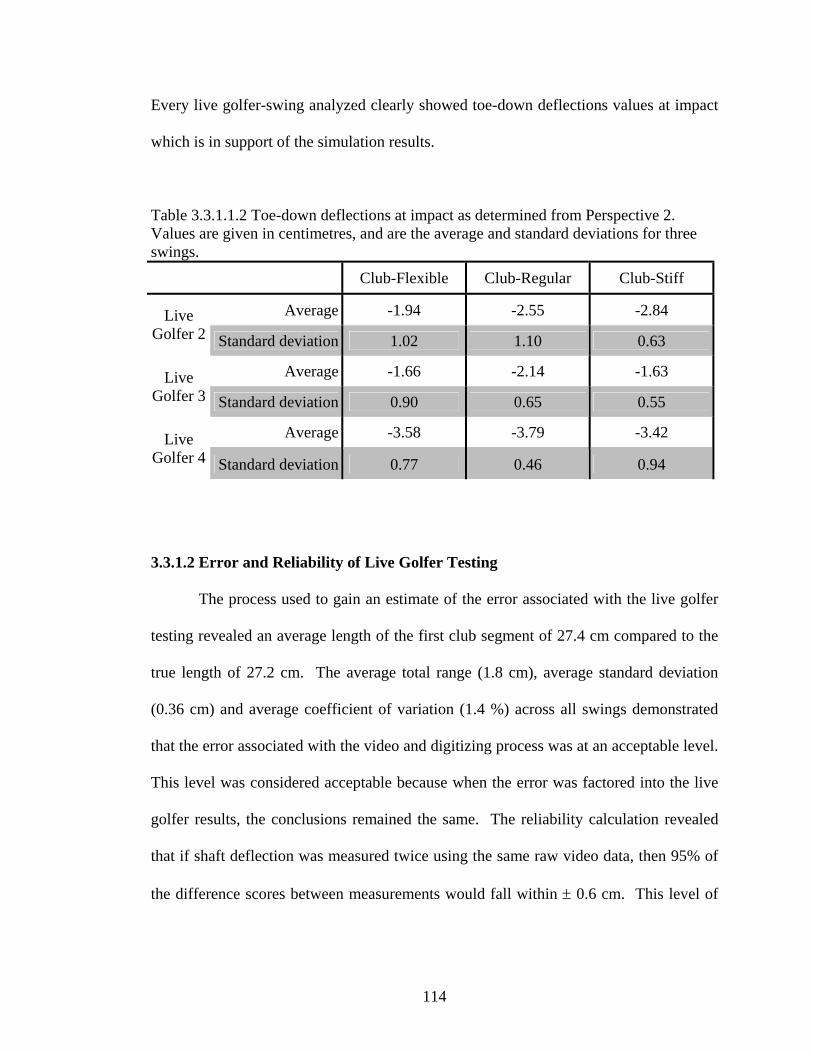
Every live golfer-swing analyzed clearly showed toe-down deflections values at impact

which is in support of the simulation results.

Table 3.3.1.1.2 Toe-down deflections at impact as determined from Perspective 2. Values are given in centimetres, and are the average and standard deviations for three swings.

Club-Flexible Club-Regular Club-Stiff

Average -1.94 -2.55 -2.84 Live Golfer 2 Standard deviation 1.02 1.10 0.63

Average -1.66 -2.14 -1.63 Live Golfer 3 Standard deviation 0.90 0.65 0.55

Average -3.58 -3.79 -3.42 Live Golfer 4 Standard deviation 0.77 0.46 0.94

3.3.1.2 Error and Reliability of Live Golfer Testing

or associated with the live golfer The process used to gain an estimate of the err

testing revealed an average length of the first club segment of 27.4 cm compared to the

true length of 27.2 cm. The average total range (1.8 cm), average standard deviation

(0.36 cm) and average coefficient of variation (1.4 %) across all swings demonstrated

that the error associated with the video and digitizing process was at an acceptable level.

This level was considered acceptable because when the error was factored into the live

golfer results, the conclusions remained the same. The reliability calculation revealed

that if shaft deflection was measured twice using the same raw video data, then 95% of

the difference scores between measurements would fall within ± 0.6 cm. This level of

114

reliability does not affect the interpretation of the live golfer testing results presented

above.

3.3.1.3 Swing Plane Comparison

Two allowances were made in the development of the model used in this thesis

which permitted the swing plane values throughout the downswing to follow the same

general pattern determined by Coleman and Rankin (2005). The first allowance was to

constrain the arm to move in a plane that was 20° steeper than the plane on which the

torso rotated. This inherently resulted in the swing plane becoming steeper as impact

approached. The second modification was to permit the arm segment to rotate about its

longitudinal axis. Implementing this degree of freedom into the model permitted the

potential for swing plane variations in either direction during the downswing. Coleman

and Rankin showed that, for a 5 iron swung by a professional golfer (Participant 1 in

their study), the swing plane showed a slight increase in angle before peaking at

approximately 138° and then steadily decreasing down to an angle of approximately

103° at impact. The swing plane angle was measured from the right horizontal, not the

left horizontal as depicted in Figure 2.1.1.2 of this thesis. Therefore, Coleman and

Rankin showed that the swing plane for Participant 1 increased in steepness by

approximately 35° throughout the downswing. The swing plane angle for the Golfer-

Medium\Club-Regular simulation also increased in steepness by approximately 35° as it

decreased from a maximum angle of 165° to an angle of 130° at impact (Fig. 3.3.1.3.1).

The swing plane angle followed the same general pattern as presented by Coleman and

Rankin (for Participant 1 who had a 0 handicap), but is consistently flatter at all points

115

during the swing. Due to the added length of the driver over a 5 iron, the swing plane

should be flatter at every stage throughout the downswing. The driver swing plane

angle for this study was in the range reported by Williams and Sih (2002). Through the

impact area, they reported a driver swing plane of 131.5 ± 3.9° which compares closely

with the swing plane measured through impact for the swing of Golfer-Medium with

Club-Regular (130.1°). Therefore, even though the golfer portion of the model was

limited to 4 degrees of freedom, it was still able to represent a varying swing plane that

is similar to that of actual golfers. Notice that the swing plane graph begins at t = 0.06 s

(Fig. 3.3.1.3.1). Coleman and Rankin started their plots of swing plane at the point

where the clubhead reversed direction at the top of the backswing. Since all simulations

in this thesis began with motion still existing in the backswing, Figure 3.3.1.3.1 was

adjusted to meet the conditions defined by Coleman and Rankin. Note: the swing plane

angle was also calculated according to the methods of Coleman and Rankin (2005).

116

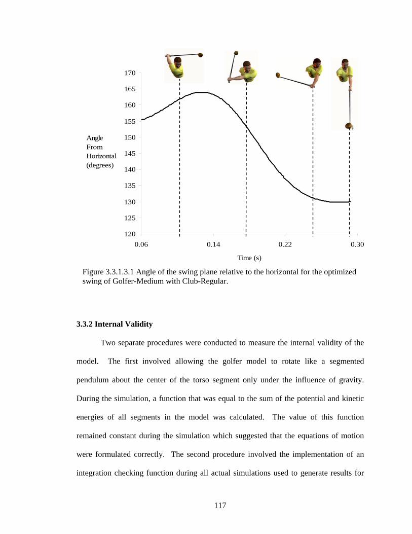
120

125

130

135

140

145

150

155

160

165

170

0.06 0.14 0.22 0.30

Time (s)

AngleFromHorizontal(degrees)

Figure 3.3.1.3.1 Angle of the swing plane relative to the horizontal for the optimized swing of Golfer-Medium with Club-Regular.

3.3.2 Internal Validity

Two separate procedures were conducted to measure the internal validity of the

model. The first involved allowing the golfer model to rotate like a segmented

pendulum about the center of the torso segment only under the influence of gravity.

During the simulation, a function that was equal to the sum of the potential and kinetic

energies of all segments in the model was calculated. The value of this function

remained constant during the simulation which suggested that the equations of motion

were formulated correctly. The second procedure involved the implementation of an

integration checking function during all actual simulations used to generate results for

117

this thesis. This integration checking function also remained at a constant value during

all simulations which implies that the model was developed correctly in accordance with

Newton’s Laws of Motion. It also confirms that the level of error introduced by the

numerical solving of the differential equations was not large enough to be a concern.

118

4

DISCUSSION

119

The purpose of this thesis was to further the understanding of the role of shaft

stiffness in executing a golf drive. A thorough set of experiments was conducted to

answer explicit questions related to this goal. Specifically, how does shaft stiffness

affect clubhead speed and how does it alter clubhead orientation at impact. Additional

experiments were performed to determine the underlying mechanisms responsible for

the pattern of shaft deflection occurring during the downswing. For the first time, a 3D

mathematical model of a golfer and club was developed and employed to answer these

questions. This discussion will integrate the results from all experiments to address the

hypotheses posed at the beginning of this thesis and to establish a comprehensive theory

that explains the pattern of shaft deflection during the downswing.

4.1 The Relationship Between Shaft Stiffness and Clubhead Speed

Customizing the stiffness of a golf club shaft to perfectly suit a particular swing

will not increase clubhead speed (and therefore ball speed) enough to have any

meaningful effect on performance. This statement is confirmed by the clubhead speed

results generated from the simulations (Table 3.1.2.1). No single shaft stiffness out

performed the other two at any level of swing speed. At any given level of swing speed,

the difference in clubhead speeds across levels of shaft stiffness did not exceed 0.1 m/s.

An attempt was made to fine tune shaft stiffness even further by matching all possible

levels of shaft stiffness with a single swing. The results indicated that regardless of

swing speed, clubhead speed increased marginally as shaft flexibility decreased.

120

Unfortunately, the marginal increases in clubhead speed were also accompanied by

unacceptable configurations of the golfer-club models at impact.

Previous studies have shown that shaft flexibility can increase clubhead speed

via the contribution from kick velocity (Butler & Winfield, 1994; Miao et al., 1998).

Even in this thesis, a kick velocity of 10.51 m/s (Table 3.1.2.1) at impact was recorded

for Golfer-Fast with Club-Regular suggesting that clubhead speed at impact would have

been reduced by 10.51 m/s if the shaft were perfectly rigid. Yet when Golfer-Fast was

matched with Club-Rigid, clubhead speed was only reduced by 1.87 m/s in comparison

to Club-Regular. Also, kick velocities at impact for Golfer-Fast/Club-Flexible (10.51

m/s) and Golfer-Fast/Club-Stiff (9.55 m/s) differed by approximately 1 m/s, yet both

simulations resulted in the same clubhead speed of 52.94 m/s at impact (Table 3.1.2.1).

These findings show that kick-velocity is a misleading variable. An understanding of

how kick velocity is produced is provided in the following paragraph and will explain

why kick velocity does not simply add on to the clubhead speed generating capabilities

of the golfer.

In an attempt to square the clubface for impact, tangential forces were applied at

the grip end of the club just past the halfway point into the downswing. This resulted in

the clubhead being deflected into a lagging position and the consequent storage of

energy in the rotational springs joining the shaft segments. This storage of energy was

accompanied by the rotational springs generating torques that tended to prevent

deflection in the lag direction and support deflection in the lead direction. As impact

approached, the tangential forces causing the lag deflection decreased which allowed the

torque from the rotational springs to deflect the clubhead from its lagging position into a

121

leading position. This could also be referred to as the release of strain energy and was

facilitated by the action of radial force which was approaching its maximum value near

impact. This process certainly increased clubhead speed relative to the most proximal

club segment. Yet, it also served to simultaneously impede the absolute angular

velocity of the most proximal club segment which was a detriment to clubhead speed.

This happened because at the same time the restoring torque of the deformed rotational

spring served to increase the angular velocity of the distal segment, an equal and

opposite torque served to decrease the angular velocity of the proximal segment.

However, the golfer model did have some ability to oppose the decrease in angular

velocity of the most proximal club segment based on the properties of the muscle torque

generators. This is evident when comparing the clubhead speeds attained with the rigid

and non-rigid clubs (Table 3.2.1.1). Since clubhead speeds were greater with the non-

rigid clubs, it shows that the shaft did have some ability to store and release energy

during the swing. However, when comparing the non-rigid clubs, no particular level of

shaft stiffness had a superior ability to increase clubhead speed, through the contribution

of kick velocity, during the simulated swings (Table 3.1.2.1).

A golfer does not have the ability to produce constant levels of acceleration

during the downswing which has important implications when considering the potential

contribution from kick velocity. Researchers have developed golfer models which

employed fixed levels of acceleration during the downswing in an attempt study shaft

flexibility (Jorgensen, 1994; Miao et al., 1998). This is not a reasonable assumption

since the golfer model must be able to interact with the dynamic properties of the club.

If fixed functions of acceleration were used in this thesis in place of the muscle torque

122

generators, then the importance of shaft flexibility in contributing to clubhead speed

would have been greatly over estimated. If the angular acceleration of the most

proximal club segment was predetermined, then the torque from the rotational springs

would only serve to increase clubhead speed and not decrease the angular velocity of the

most proximal club segment. This would result in spuriously large clubhead speeds. It

is also likely that golfer robots may suffer from this same limitation; namely, the

inability to dynamically interact with the properties of a golf club in the same way as a

live golfer.

Currently, no researcher has presented conclusive results showing that different

shaft flexibilities result in measurably higher clubhead speeds at impact and therefore,

subsequently higher ball speeds. Miao et al. (1998) presented data which suggested that

certain levels of shaft stiffness resulted in higher clubhead speeds for a particular golfer.

However, as previously indicated in this thesis, it appears as though the error levels

associated with the data presented by Miao et al. were greater then the differences that

were measured in clubhead speeds across levels of shaft stiffness.

Based on the previous arguments it should not be inferred that certain levels of

shaft stiffness cannot outperform others for a particular swing when considering

increased driving yardage. Rather it should be understood that if driving distance was

found to be meaningfully different across levels of shaft stiffness, then that increased

driving yardage would be a result of factors other then differences in ball speed. These

other factors, namely, ball launch angle and ball spin rate are influenced by clubhead

orientation at impact which is in turn determined by shaft deflection.

123

4.2 The Relationship Between Shaft Stiffness and Clubhead Orientation

Aside from golf ball speed which is primarily a function of clubhead speed, ball

launch angle and spin rate are the only other two factors under the control of the golfer

that can affect driving distance. For a perfectly impacted golf ball, no side spin is

imparted to the ball and the flight of the ball does not deviate from a path directly above

the target line. Under these conditions, launch angle refers to the angle between the

velocity vector of the ball and the horizontal immediately after impact, while spin rate

refers to the amount of angular velocity (back spin) imparted to the ball. With respect to

the execution of a golf drive, spin rate is primarily a function of clubhead loft (including

dynamic loft), while launch angle is a function of both clubhead loft and clubhead path

(Winfield & Tan, 1994). If a golfer has a consistent swing, then the path of the clubhead

relative to the ball will not change from swing to swing. Therefore, by adjusting the

amount of clubhead loft relative to the ball, an optimal ball launch angle and ball spin

rate can be found for achieving maximum driving distance. Results from the computer

simulations demonstrated that clubhead loft can change by as much as 0.65° depending

on shaft stiffness for a golfer with a swing speed of approximately 45 m/s (101 mph)

(Table 3.1.2.1). For example, the Golfer-Medium\Club-Stiff simulation resulted in

4.82° of dynamic loft at impact, while the Golfer-Medium\Club-Flexible simulation

resulted in 5.47° of dynamic loft. The results from the optimization study conducted by

Winfield and Tan suggest that a loft change of this magnitude may be enough to have a

meaningful influence on driving distance. However a golfer must swing very

consistently to take advantage of these changes. Also, larger differences in clubhead

124

loft could be expected when comparing the non-optimized swings of many amateur

golfers.

It should also be pointed out that the loft increases brought about as a result of

shaft flexibility could also be made simply by changing the static loft of the club. For

example, clubhead loft dynamically increased by 0.65° when Golfer-Regular was

matched with Club-Flexible (5.47°) in comparison to the Golfer-Regular\Club-Stiff

(4.82°) combination (Table 3.1.2.1). These two simulations would theoretically produce

different ball flight conditions because of the discrepancy in clubhead loft at impact. If

the face angle of Club-Stiff was geometrically changed to increase the static loft of the

club by 0.65°, both conditions would then produce the same theoretical ball flight. This

would be the case because the clubhead paths between conditions were already not

meaningful different (not previously reported), and the clubhead speeds were already

very similar (44.96 m/s vs. 45.04 m/s). The effect of statically changing the loft of

clubface was confirmed using the model. Statically increasing the loft from 10° to

10.65° resulted in the loft at impact increasing by 0.6496°. Physically altering the loft

of the clubface will not change the position of the center of mass of the clubhead and

therefore, will have no influence on shaft deflections during the swing.

In summary, clubhead path, loft and speed influence ball flight. As a variable,

only shaft stiffness was found to have a meaningful effect on clubhead loft which can

also be changed by altering the physical geometry of the club. Therefore, it seems that

shaft stiffness is not a necessary variable to consider when fitting a driver to a golfer’s

swing.

125

However, there are two other factors to consider before defining the role of shaft

stiffness. First, perhaps solely manufacturing a more complete spectrum of clubhead

geometries with a single shaft stiffness is not practical. It may be more economically

feasible for club manufacturers to provide a range of both clubhead geometries and shaft

stiffness that produce the desired impact conditions. Second, the influence of feel

cannot be easily dismissed. Certainly, the feel of the driver is linked to the golfer’s

confidence in executing the shot which will inevitably weigh heavy on the final outcome

of the swing.

4.3 The Mechanisms Behind Shaft Bending

Both radial and tangential forces, relative to the circular path traced by the

longitudinal axis of the shaft, played important roles in shaft deflection during the

downswing and in the resulting clubhead orientation at impact. The possible

mechanisms behind shaft bending were previously discussed in the introduction. It was

argued that using a conceptual frame work that described forces that were either radial

or tangential to the longitudinal axis of the shaft would help understand the cause of

shaft deflection during the downswing. The same conceptual frame work will be used

in this discussion.

The largest magnitude of shaft deflection during the downswing was in the toe-

up direction. For the computer simulation swings of Golfer-Medium, the maximum toe-

up deflections were approximately 10 cm in magnitude and occurred during the initial

part of the downswing. Tangential forces acting along the x axis were the primary cause

of these deflections. Contrary to popular belief, this initial deflection had no impact on

126

clubhead speed and little influence on the final orientation of the clubface at impact.

Initial bending in the toe-up direction may superficially appear to be storing energy

which could later be released to increase clubhead speed. However, due to the 90°

rotation of the club about the lead arm during the final stage of the downswing, none of

the energy stored in the initial part of the swing could ever be returned to the clubhead

along the intended direction of ball flight. Further, any residual effects of this deflection

present at impact will only have a small effect on the dynamic loft of the club. Based on

the results of this thesis, it would appear that the initial bending in the toe-up direction

would only serve to increase the variability in a golf swing. This information supports

the view of those golf instructors that advocate a ‘smooth’ transition into the

downswing, as opposed to a rushed transition that would lead to larger shaft deflections

early in the downswing.

The next important period of shaft deflection occurred in the lag direction over

the final half of the downswing. For the computer simulation swings of Golfer-

Medium, the maximum lag deflections were approximately 3.5 cm in magnitude.

Tangential forces, acting along the y axis were the primary cause of deflections in the

lag direction. Shaft deflection in this direction resulted in the storage of strain energy

that had the potential to be released near impact and result in a faster clubhead speed.

This period of shaft deflection cannot be predicted from a 2D model and is essentially

why a 3D simulation was needed to sufficiently model the downswing.

The final phase of shaft deflection was the most important since it described

clubhead orientation at impact. It was also the most complex because both tangential

and radial forces played meaningful roles, and because it occurred over a relatively short

127

time period (0.03 s). Over the final few hundredths of a second of the downswing, the

clubhead rapidly moved from its maximum lagging position into its maximum leading

position at impact. For the computer simulation swings of Golfer-Medium, the lead

deflections at impact were approximately 6.0 to 6.5 cm in magnitude. The complete

removal of radial force during the downswing only reduced lead deflection to 4.72 cm

(Fig. 3.2.3.1). Therefore, when acting in isolation, the tangential forces were

responsible for a considerable portion of the lead deflection at impact. The complete

isolation of radial force demonstrated that while acting alone, radial force could only

result in 1.22 cm of lead deflection at impact (Fig. 3.2.3.2). Summing the lead

deflection that occurred from the isolation of the two sets of forces results in a lead

deflection of 5.94 cm, which is 0.31 cm less than when radial and tangential forces acted

simultaneously. This finding suggests that there is an interaction effect between the

force components in terms of lead deflection.

Toe-down deflection at impact was also affected by both radial and tangential

force components. Both radial and tangential force components contributed

approximately equally to the magnitude of toe-down deflection at impact. When acting

in isolation, radial force was shown to deflect Club-Regular by -1.33 cm in the toe-down

direction. For the optimized swing of Golfer-Medium with Club-Regular, toe-down

deflection was -2.26 cm at impact; therefore, just over half of that deflection was the

direct result of radial force action. The additional deflection was the result of the club

recoiling from its toe-up deflected position earlier in the downswing.

128

4.4 The Role of Radial Force

Several researchers claim that radial force is the dominant factor producing shaft

deflection at impact (Mather & Cooper, 1994; Butler & Winfield, 1994, Horwood, 1994;

Milne & Davis, 1992; Mather & Jowett, 1998). The results from section 3.2.3

demonstrated that when radial force acted in isolation, shaft deflection in either the toe-

down or lead direction did not exceed 1.33 cm in magnitude. Yet, several authors

(Mather & Cooper, 1994; Butler & Winfield, 1994, Horwood, 1994), as well as, the

results from this thesis have demonstrated that shaft deflection at impact can exceed 4

cm in both directions. A possible explanation of these ambiguous findings is that the

radial force generated by the model used in this thesis was not large enough to produce

the previously reported magnitudes of shaft deflection.

However, the peak magnitude of radial force (456 N) measured during the

optimized swing (45 m/s) of Golfer-Medium with Club-Regular was within the range

presented in the literature. Williams (1967) deduced that Bobby Jones generated a

clubhead speed of approximately 50 m/s and applied a radial force of 476 N to his driver

at impact. Vaughn (1981) (360 N) and Neal and Wilson (1985) (315 N) reported

reduced values for peak radial force during the downswing. However, these researchers

generated their results from 3D inverse dynamic analyses of live golfers which bring

into question how much their smoothing techniques reduced peak values. Miura (2001)

predicted a radial force of 414 N from his 2D model which generated a clubhead speed

of 46.8 m/s. Mather and Jowett (1998), state that radial force approaches 500 N for

clubhead speeds of 45 m/s. Considering these results, it appears as though 456 N is a

reasonable prediction of radial force.

129

Another possible explanation is that the simulated clubs used in this thesis were

too stiff to permit radial force to generate the previously reported magnitudes of shaft

deflection. This explanation seems doubtful when the peak magnitudes of shaft

deflection in the toe-up direction, and lag direction are compared to previous research.

Butler and Winfield (1994) reported peak toe-up deflections (15 cm) and peak lag

deflections (7 cm), that were greater than the respective measurements from the

simulation results in this thesis (10.69 cm and 4.79 cm). Milne and Davis (1992) also

reported peak toe-up deflections exceeding 10 cm in magnitude.

In summary, radial force plays an important role in facilitating the toe-down and

lead-deflections recorded in all ‘golf’ swings made with a driver. However, the recoil of

the shaft from its previously toe-up and lag deflected position, due to tangential forces,

plays at least an equally important role in determining the final position and orientation

of the clubhead.

4.5 Limitations of the Model

As all models do, the mathematical model used in this thesis did not completely

represent every aspect of the target system. The purpose of this section is to address the

limitations of the mathematical model.

The role of the golfer portion of the mathematical model was to apply a realistic

temporal pattern of forces and torques to the grip end of the club model. The two

segment golfer representation employed to fulfil this role was able to reproduce most of

the motion of a live golfer. The fact that the torso segment was constrained to rotate

around a fixed axis meant that the linear motion of the trunk, that might result from the

leg action of a live golfer, was not represented in the model. The lack of linear motion

130

in the trunk was not regarded as a major limitation since the golf swing is predominantly

rotational. However, due to the lack of direct leg musculature contribution, it was likely

that the outputs from the muscle torque generators were slightly greater than that of a

live golfer with a similar clubhead speed. Related to the absence of legs from the model

is the absence of hip rotation. It is generally agreed upon that the first movement into

the downswing is hip rotation. In the popular golfing literature, a large difference in

angular rotation between the hips and shoulders early in the downswing is often cited as

a good indicator of a properly executed swing. The absence of a pelvic girdle in the

model simply means the absence of another segment which could contribute to the

overall motion. This would also likely lead to slightly greater muscle torque outputs.

The golfer model used in this thesis also incorporated any contribution from a trail arm

into the wrist adductor of the lead arm. It is possible that this representation may have

influenced the clubhead speed results from section 3.1.. It was determined in section 3.1

that, for a given golfer, altering the stiffness of a golf shaft would have no meaningful

effect on clubhead speed. This was the result of the golfer model dynamically

interacting with the torques produced by the spring-damper elements of the shaft. The

torques from the spring-damper elements served to increase kick velocity while

simultaneously reducing the angular velocity of the most proximal club segment. It is

possible that incorporating a trail arm into the model may have offset the effect of the

bending moments in the shaft on the most proximal club segment’s angular velocity.

However, I feel that this is not likely for two reasons. First, the torque generating

capabilities of the wrist adductor were increased to represent both the wrist adductor and

trail arm contributions to the downswing. Second, the torques responsible for increases

131

in kick velocity occurred very late in the downswing. This would place the trail arm in a

compromised position from which to apply forces to the club.

Although, the muscle representation used in the golfer model is more

encompassing than those used in previous golfer models, it does not match the

complexity of similar models used to simulate jumping and walking. Essentially the

potential limitations of the muscle models are that they represent overall joint moments

and not individual muscle forces, neural inputs were not incorporated, and the length-

tension property of muscle was not modelled. The important question is how do these

simplifications affect the pattern of forces and torques experienced by the golf club?

Employing individual muscle models is important if the purpose of the research

is to understand the role of individual muscles to the overall movement pattern. This is

often the case in studies that model jumping. However, if the purpose is merely to

generate an accurate representation of the real system’s kinematic pattern, then torque

generators are sufficient. Therefore, the lack of individual muscle force representation

has little bearing on the results generated to investigate the hypotheses posed in this

thesis. From the viewpoint of the golf club, it makes no difference if four separate

muscle force generators add energy into the arm segment, or if that role is fulfilled by a

single muscle torque generator. The resulting motion of the golfer model and

consequently the kinetics imposed on the club remain the same.

Incorporating neural stimulation into the model allows graded levels of

“muscular effort” to be achieved during the simulation. This is obviously important in

models such as walking in which muscular effort is always supplied to the skeletal

system at sub- maximal levels. However, one goal for a golf drive is to displace the golf

132

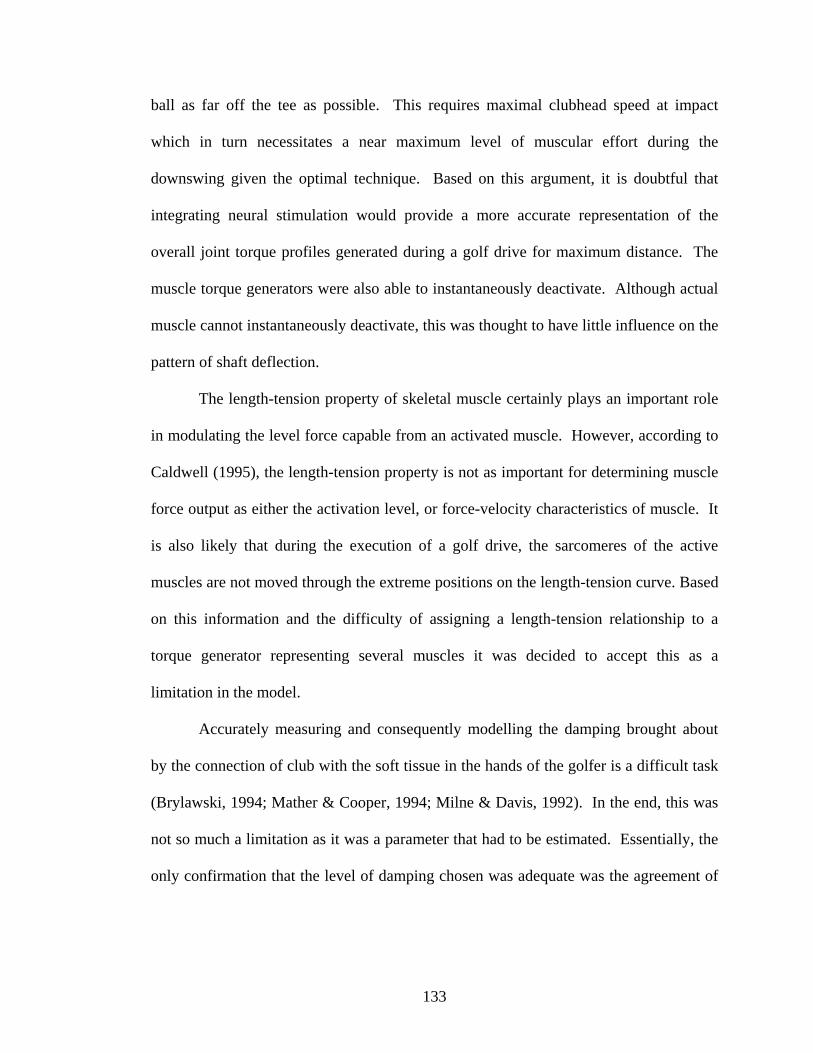
ball as far off the tee as possible. This requires maximal clubhead speed at impact

which in turn necessitates a near maximum level of muscular effort during the

downswing given the optimal technique. Based on this argument, it is doubtful that

integrating neural stimulation would provide a more accurate representation of the

overall joint torque profiles generated during a golf drive for maximum distance. The

muscle torque generators were also able to instantaneously deactivate. Although actual

muscle cannot instantaneously deactivate, this was thought to have little influence on the

pattern of shaft deflection.

The length-tension property of skeletal muscle certainly plays an important role

in modulating the level force capable from an activated muscle. However, according to

Caldwell (1995), the length-tension property is not as important for determining muscle

force output as either the activation level, or force-velocity characteristics of muscle. It

is also likely that during the execution of a golf drive, the sarcomeres of the active

muscles are not moved through the extreme positions on the length-tension curve. Based

on this information and the difficulty of assigning a length-tension relationship to a

torque generator representing several muscles it was decided to accept this as a

limitation in the model.

Accurately measuring and consequently modelling the damping brought about

by the connection of club with the soft tissue in the hands of the golfer is a difficult task

(Brylawski, 1994; Mather & Cooper, 1994; Milne & Davis, 1992). In the end, this was

not so much a limitation as it was a parameter that had to be estimated. Essentially, the

only confirmation that the level of damping chosen was adequate was the agreement of

133

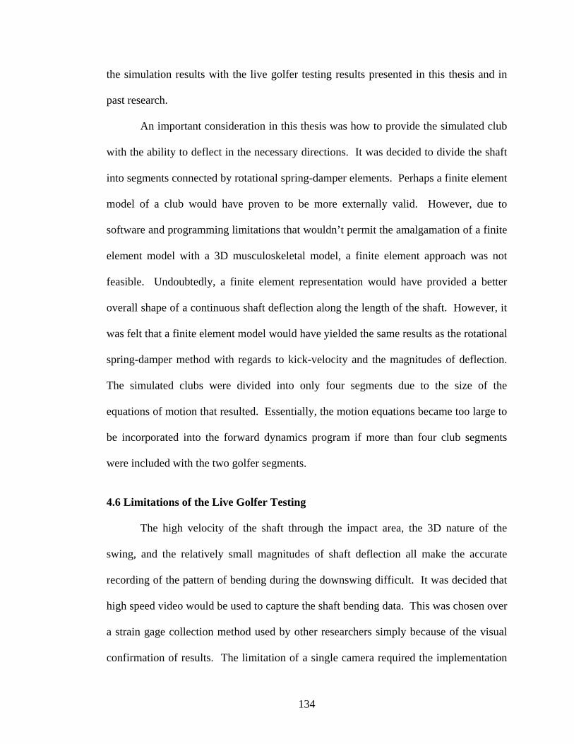
the simulation results with the live golfer testing results presented in this thesis and in

past research.

An important consideration in this thesis was how to provide the simulated club

with the ability to deflect in the necessary directions. It was decided to divide the shaft

into segments connected by rotational spring-damper elements. Perhaps a finite element

model of a club would have proven to be more externally valid. However, due to

software and programming limitations that wouldn’t permit the amalgamation of a finite

element model with a 3D musculoskeletal model, a finite element approach was not

feasible. Undoubtedly, a finite element representation would have provided a better

overall shape of a continuous shaft deflection along the length of the shaft. However, it

was felt that a finite element model would have yielded the same results as the rotational

spring-damper method with regards to kick-velocity and the magnitudes of deflection.

The simulated clubs were divided into only four segments due to the size of the

equations of motion that resulted. Essentially, the motion equations became too large to

be incorporated into the forward dynamics program if more than four club segments

were included with the two golfer segments.

4.6 Limitations of the Live Golfer Testing The high velocity of the shaft through the impact area, the 3D nature of the

swing, and the relatively small magnitudes of shaft deflection all make the accurate

recording of the pattern of bending during the downswing difficult. It was decided that

high speed video would be used to capture the shaft bending data. This was chosen over

a strain gage collection method used by other researchers simply because of the visual

confirmation of results. The limitation of a single camera required the implementation

134

of separate set-ups to measure shaft bending in both the toe-down/toe-up and lead/lag

directions. This was not ideal since deflection data for both bending directions could

not be obtained from a single swing. The set-up from Perspective 2 with the camera

behind the golfer would also not permit the determination of clubhead speed for those

trials. This meant that a relationship between toe-down deflection and clubhead speed

could not be analyzed.

4.7 Conclusions

The following conclusions address the purpose and hypotheses stated in the

introduction to this thesis and are based on the results that emerged from the

experiments described in the methods section.

(1) A six-segment, 3D mathematical model of a golfer driven by muscle torque

generators can be successfully used to model the behaviour of a golf shaft

during the downswing. This supports hypothesis 1.

(2) Tangential forces applied by the golfer to the club handle are the major

contributors to the shaft deflections that occur during the first 90% of the

downswing. Tangential forces play at least an equally important role as

radial force in determining the final deflected position of the club at impact.

This supports hypothesis 2.

135

(3) Radial force serves to increase the magnitudes of the toe-down and lead

deflections present at impact during optimal swings with a driver.

(4) The simulation results showed that the flexibility of a golf shaft has no

influence on clubhead speed for golfers of different swing speed capabilities.

The supports hypothesis 3.

(5) All optimal golf swings with a driver will result in the shaft being deflected

in the toe-down and lead directions at impact. For golf swings with a similar

pattern of force and torque application to the club, as swing speed increases

so does the magnitude of shaft deflection at impact. This supports

hypothesis 4.

(6) For an optimal golf swing, as shaft stiffness decreases the magnitude of shaft

deflection at impact increases. This supports hypothesis 4.

(7) Altering the position of the center of mass of the clubhead affects clubhead

orientation at impact by an amount proportional to the size of the change in

position. The change in clubhead orientation associated with altering the

center of mass of the clubhead is a result of the action of radial force. This

supports hypothesis 5.

136

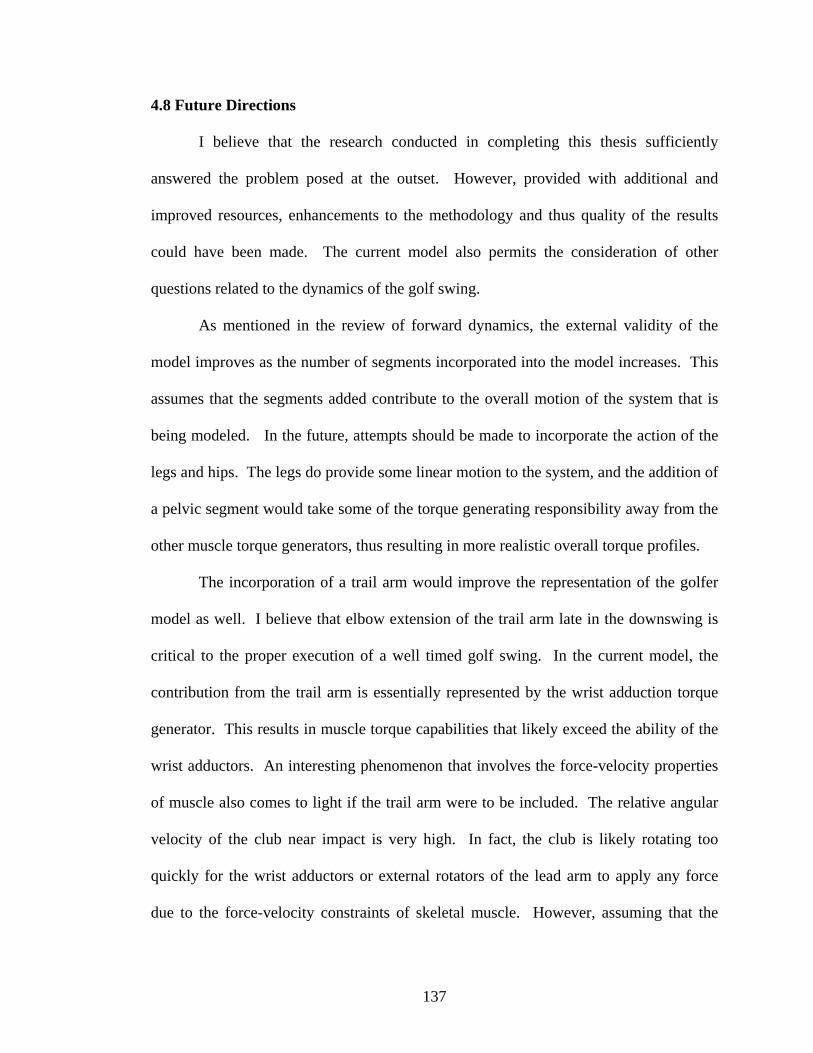
4.8 Future Directions

I believe that the research conducted in completing this thesis sufficiently

answered the problem posed at the outset. However, provided with additional and

improved resources, enhancements to the methodology and thus quality of the results

could have been made. The current model also permits the consideration of other

questions related to the dynamics of the golf swing.

As mentioned in the review of forward dynamics, the external validity of the

model improves as the number of segments incorporated into the model increases. This

assumes that the segments added contribute to the overall motion of the system that is

being modeled. In the future, attempts should be made to incorporate the action of the

legs and hips. The legs do provide some linear motion to the system, and the addition of

a pelvic segment would take some of the torque generating responsibility away from the

other muscle torque generators, thus resulting in more realistic overall torque profiles.

The incorporation of a trail arm would improve the representation of the golfer

model as well. I believe that elbow extension of the trail arm late in the downswing is

critical to the proper execution of a well timed golf swing. In the current model, the

contribution from the trail arm is essentially represented by the wrist adduction torque

generator. This results in muscle torque capabilities that likely exceed the ability of the

wrist adductors. An interesting phenomenon that involves the force-velocity properties

of muscle also comes to light if the trail arm were to be included. The relative angular

velocity of the club near impact is very high. In fact, the club is likely rotating too

quickly for the wrist adductors or external rotators of the lead arm to apply any force

due to the force-velocity constraints of skeletal muscle. However, assuming that the

137

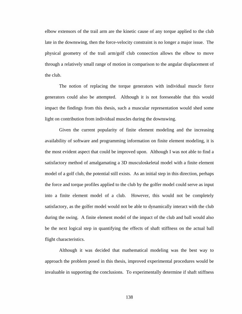
elbow extensors of the trail arm are the kinetic cause of any torque applied to the club

late in the downswing, then the force-velocity constraint is no longer a major issue. The

physical geometry of the trail arm/golf club connection allows the elbow to move

through a relatively small range of motion in comparison to the angular displacement of

the club.

The notion of replacing the torque generators with individual muscle force

generators could also be attempted. Although it is not foreseeable that this would

impact the findings from this thesis, such a muscular representation would shed some

light on contribution from individual muscles during the downswing.

Given the current popularity of finite element modeling and the increasing

availability of software and programming information on finite element modeling, it is

the most evident aspect that could be improved upon. Although I was not able to find a

satisfactory method of amalgamating a 3D musculoskeletal model with a finite element

model of a golf club, the potential still exists. As an initial step in this direction, perhaps

the force and torque profiles applied to the club by the golfer model could serve as input

into a finite element model of a club. However, this would not be completely

satisfactory, as the golfer model would not be able to dynamically interact with the club

during the swing. A finite element model of the impact of the club and ball would also

be the next logical step in quantifying the effects of shaft stiffness on the actual ball

flight characteristics.

Although it was decided that mathematical modeling was the best way to

approach the problem posed in this thesis, improved experimental procedures would be

invaluable in supporting the conclusions. To experimentally determine if shaft stiffness

138

could meaningful influence clubhead speed, several conditions would have to be met.

Professional golfers with highly repeatable swings would have to be employed. As in

this study, golf clubs identical in all aspects with the exception of shaft stiffness would

need to be incorporated. Perhaps most import, very accurate measurements of golfer

motion and clubhead speed would have to be recorded over many trials. The

measurements would have to be extremely accurate (± 2 mm). The data collection

system would also need a very high sampling rate (at least 500 Hz), and be able to track

the complicated 3D motion of the club in a relatively large volume. With this

experimental set-up, a researcher should be able to ascertain whether clubhead speed

can be influenced by shaft stiffness.

Although not related to the purpose, a very interesting finding occurred in the

development of the 3D golfer-club model used in this thesis. This finding, which I will

explain below, not only provides an important direction for future investigation, but also

serves as an excellent anecdote on the advantages and even necessity of forward

dynamic models.

The kinematics of the golf swing are relatively complex. The kinetics that

produced the kinematics are, in my opinion, inherently more complex. In considering

the optimal execution of a skill requiring musculoskeletal motion, the researcher or

individual instructing the skill is interested in what the performer must do to execute the

skill. More explicitly, what contributions from the muscles of the performer are

necessary to attain the observed optimal kinematics? This is not necessarily obvious

from the measured kinematics. For example, an individual with a below the knee

prosthesis is still able to perform knee flexion and extension movements during walking

139

without any contribution from muscles crossing the knee. These motions are caused by

the joint reaction forces at the knee and the resulting momentum. Similar principles are

at work in the golf swing, but are much more difficult to visualize than the prosthetic

example just described, due to the high velocity and 3D nature of the swing. A forward

dynamics model permits the deciphering of what motions result from the “passive

forces” occurring during the golf swing, and those motions which are a direct result of

muscular action. This information is essential to teaching and the correct execution of a

golf swing. The following describes such a finding that emerged from the development

of the golfer model used in this thesis.

The muscle torque generators present in the golfer model can directly generate

four basic movements. Three of those movements: torso rotation, shoulder abduction,

and wrist adduction can move the golf club through the downswing, to the point of

impact, but cannot directly cause the clubface to square up for impact (Fig. 4.7.1 A, B,

C, D and E). The fourth movement, rotation of the lead arm about its longitudinal axis,

would appear on first inspection to provide the only mechanism to actively square up the

clubface for impact (Fig. 4.7.1 F).

140

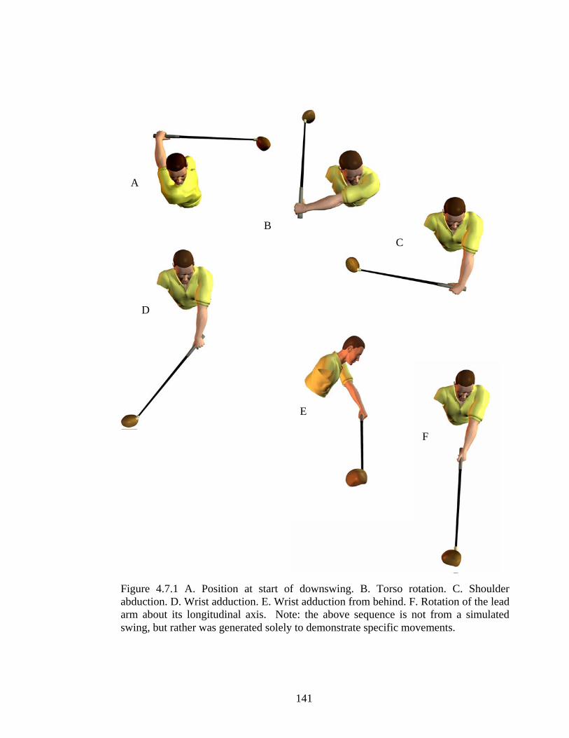
A

B C

D

E

F

Figure 4.7.1 A. Position at start of downswing. B. Torso rotation. C. Shoulder abduction. D. Wrist adduction. E. Wrist adduction from behind. F. Rotation of the lead arm about its longitudinal axis. Note: the above sequence is not from a simulated swing, but rather was generated solely to demonstrate specific movements.

141

However, in the development of the golfer model it was determined that, during

the execution of a golf drive, a torque acting about the longitudinal axis of the lead arm

was not necessary to square to the clubface for impact. Obviously, rotation about the

longitudinal axis of the lead arm was still required, but this rotation did not occur due to

a torque produced by a muscle torque generator. Rather, joint reaction forces and

gravity were the kinetic factors behind the squaring of the clubhead for impact.

Consider a golfer model that has muscle torque generators that would produce the

movements described in the Figure 4.7.1 with the exception of a torque generator that

would produce rotation about the longitudinal axis of the lead arm. The arm is free to

rotate about its longitudinal axis, but no torque generator acts about its longitudinal axis

of the lead arm. Since gravity acts at an angle to the plane in which shoulder abduction

occurs, it will tend to cause rotation about the longitudinal axis of the lead arm due to

the position of the club’s center of mass (Fig. 4.7.2A). This gravitational force results in

the club ‘falling’ below the arm abduction plane (Fig. 4.7.2B). Due to this position

inside the plane, a force acting at the grip end of the club, and within the arm abduction

plane, produces a torque on the club about the longitudinal axis of the lead arm. This

torque will act until the center of mass of the club moves within the arm abduction

plane. As the center of mass moves towards the arm abduction plane, the angular

impulse generated by the torque creates angular momentum about the longitudinal axis

of the lead arm. It is this angular momentum about the longitudinal axis of the lead arm

that caused the clubhead to square for impact in absence of muscle torque acting about

the longitudinal axis of the lead arm. Certainly, a properly timed muscle torque acting

142

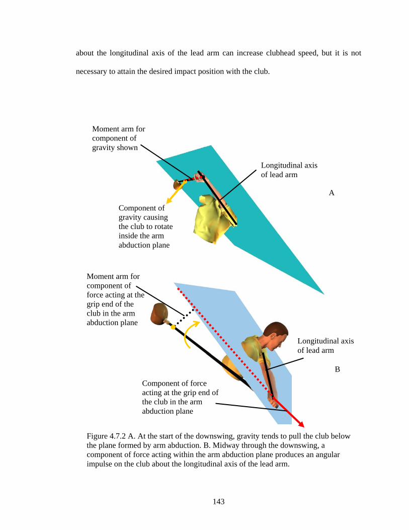
about the longitudinal axis of the lead arm can increase clubhead speed, but it is not

necessary to attain the desired impact position with the club.

Moment arm for component of gravity shown

Longitudinal axis of lead arm

Figure 4.7.2 A. At the start of the downswing, gravity tends to pull the club below the plane formed by arm abduction. B. Midway through the downswing, a component of force acting within the arm abduction plane produces an angular impulse on the club about the longitudinal axis of the lead arm.

A

Component of gravity causing the club to rotate inside the arm abduction plane

Moment arm for component of force acting at the grip end of the club in the arm abduction plane

Longitudinal axis of lead arm

B

Component of force acting at the grip end of the club in the arm abduction plane

143

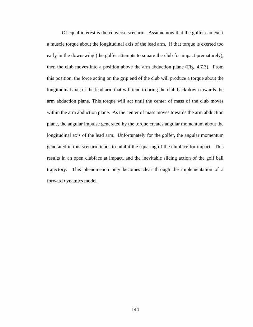
Of equal interest is the converse scenario. Assume now that the golfer can exert

a muscle torque about the longitudinal axis of the lead arm. If that torque is exerted too

early in the downswing (the golfer attempts to square the club for impact prematurely),

then the club moves into a position above the arm abduction plane (Fig. 4.7.3). From

this position, the force acting on the grip end of the club will produce a torque about the

longitudinal axis of the lead arm that will tend to bring the club back down towards the

arm abduction plane. This torque will act until the center of mass of the club moves

within the arm abduction plane. As the center of mass moves towards the arm abduction

plane, the angular impulse generated by the torque creates angular momentum about the

longitudinal axis of the lead arm. Unfortunately for the golfer, the angular momentum

generated in this scenario tends to inhibit the squaring of the clubface for impact. This

results in an open clubface at impact, and the inevitable slicing action of the golf ball

trajectory. This phenomenon only becomes clear through the implementation of a

forward dynamics model.

144

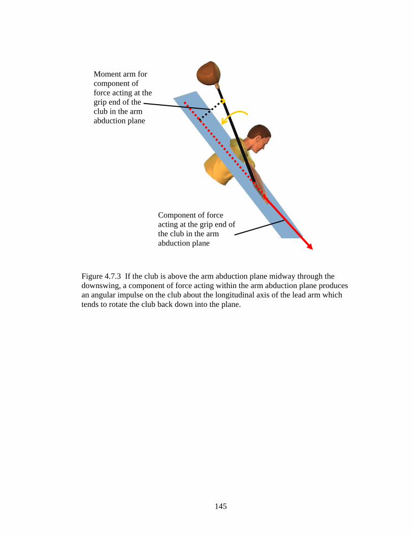
Moment arm for component of force acting at the grip end of the club in the arm abduction plane

Component of force acting at the grip end of the club in the arm abduction plane

Figure 4.7.3 If the club is above the arm abduction plane midway through the downswing, a component of force acting within the arm abduction plane produces an angular impulse on the club about the longitudinal axis of the lead arm which tends to rotate the club back down into the plane.

145

REFERENCES

Allard, P., Stokes, I. A. F., & Blanchi, J. P. (1995). Three-dimensional analysis

of human movement. Champaign, IL: Human Kinetics.

Altman D. G., & Bland, J. M. (1983). Measurement in medicine: the analysis

of method comparison studies. Statistician, 32, 307-317.

Andrews, J. G. (1995). Euler’s and Lagrange’s Equations for linked rigid-body

models of three dimensional human motion. Chapter 8 in Three-dimensional analysis of

human movement. Allard, P., Stokes, I. A. F., & Blanchi, J. P. (Eds). Champaign, IL:

Human Kinetics.

Atkinson, G., & Nevill, A. M. (1998). Statistical methods for assessing

measurement error (reliability) in variables relevant to sports medicine. Sports

Medicine, 26, 217-238.

Brylawski, A. M. (1994). An investigation of three dimensional deformation of a

golf club. In M. R. Farrally, & A. J. Cochran (Ed.), Science and Golf II: Proceedings of

the World Scientific Congress of Golf (pp. 265-270). United Kingdom: E & FN Spon.

Butler, J. H., & Winfield, D. C. (1994). The dynamic performance of the golf

shaft during the downswing. In M. R. Farrally, & A. J. Cochran (Ed.), Science and Golf

146

II: Proceedings of the World Scientific Congress of Golf (pp. 259-264). United

Kingdom: E & FN Spon.

Caldwell, G. (1995). Tendon elasticity and relative length: effects on Hill two-

component muscle model. Journal of Applied Biomechanics, 11, 1-24.

Cavanga, G. A., Citterio, G. (1974). Effect of stretching on the elastic

characteristics and the contractile component of frog striated muscle. Journal of

Physiology, 239, 1-14.

Cochran, A. J., & Stobbs, J. (1968). The search for the perfect swing. London:

Morrison & Gibb Ltd.

Coleman, S. G. S., & Rankin, A.J. (2005). A three-dimensional examination of

the planar nature of the golf swing. Journal of Sports Sciences, 23, 227-234.

Cooper, M. A. J., & Mather, J. S. B. (1994). Categorization of golf swings. In M.

R. Farrally, & A. J. Cochran (Ed.), Science and Golf II: Proceedings of the World

Scientific Congress of Golf (pp. 65-70). United Kingdom: E & FN Spon.

De Leva, P. (1996). Adjustments to Zatsiorsky-Seluyanov’s segment inertia

parameters. Journal of Biomechanics, 29, 1223-1230.

147

Dudel, J. (1978). In R. Schmidt (Ed.), Fundamentals of Neurophysiology 2nd

Edition. New York: Springer-Verlag.

Edman, K. A., Elzinga, G., & Noble, M. I. (1978). Enhancement of mechanical

performance by stretch during titanic contraction of vertebrate skeletal muscle fibres.

Journal of Physiology, 281, 139-155.

Fox, L. (1962). Numerical solutions of ordinary and partial differential

equations. (pp. 24-25). Palo Alto: Addison-Wesley.

Hanavan, E. P. (1964). A mathematical model of the human body. Report no.

AMRL-TR-64-102, AD-608-463. Ohio: Aerospace Medical Research Laboratories,

Wright-Patterson Air Force Base.

Hatze, E. (1980). A mathematical model for the computational determination of

parameter values of anthropometric segments. Journal of Biomechanics, 13, 833-843.

Hill, A. V. (1938). The heat of shortening and the dynamic constants of muscle.

Proceedings of the Royal Society, 126B, 136-195.

Hill, A. V. (1970). First and Last Experiments in Muscle Mechanics. London:

Cambridge University Press.

148

Hogarth, K. L. (2002). An analysis of twisting dives. Ph.D. Thesis, The

University of Queensland, Brisbane, Queensland, Australia.

Horwood, G. P. (1994). Golf shafts – a technical perspective. In M. R. Farrally,

& A. J. Cochran (Ed.), Science and Golf II: Proceedings of the World Scientific

Congress of Golf (pp. 247-258). United Kingdom: E & FN Spon.

Houk, J. C. (1963). A mathematical model of the stretch reflex in human muscle

systems. M.S. Thesis, M.I.T., Cambridge MA.

Huxley, A. F. (1974). Muscular contraction. Journal of Physiology, 243, 1-43.

Jorgensen, T. P. (1994). The physics of golf. USA: AIP Press.

Jorgensen, T. P. (1970). On the dynamics of the swing of a golf club. American

Journal of Physics, 38, 644-651.

Kirsch, B. G. (1998). The Americanization of golf: 1888-1914. In M. R.

Farrally, & A. J. Cochran (Ed.), Science and Golf III: Proceedings of the World

Scientific Congress of Golf (pp. 331-336). United Kingdom: Human Kinetics.

149

Lampsa, M. (1975). Maximal distance of the golf drive: an optimal control

study. Journal of Dynamic Systems, Measurement, and Control Transactions. ASME,

362-367.

Mather, J. S. B., Jowett, S. (1998). The effect of centrifugal stiffening on the

bending stiffness of a golf shaft. In M. R. Farrally, & A. J. Cochran (Ed.), Science and

Golf III: Proceedings of the World Scientific Congress of Golf (pp. 515-521). United

Kingdom: Human Kinetics.

Mather, J. S. B., Smith, M. J., Jowett, S., Gibson, K. A. H., & Moynihan, D.

(2000). Application of a photogrammetric technique to golf club evaluation. Sports

Engineering, 3, 37-47.

Mather, J. S. B., & Cooper, M. A. J. (1994). The attitude of the shaft during the

swing of golfers of different ability. In M. R. Farrally, & A. J. Cochran (Ed.), Science

and Golf II: Proceedings of the World Scientific Congress of Golf (pp. 271-277).

United Kingdom: E & FN Spon.

Miao, T., Watari, M., Kawaguchi, M., & Ikeda, M. (1998). A study of clubhead

speed as a function of grip speed for a variety of shaft flexibility. In M. R. Farrally, &

A. J. Cochran (Ed.), Science and Golf III: Proceedings of the World Scientific Congress

of Golf (pp. 554-561). United Kingdom: Human Kinetics.

150

Miura, K. (2001). Parametric acceleration - the effect of inward pull of the golf

club at impact stage. Sports Engineering, 4, 75-86.

Michalewicz, Z. (1996). Genetic algorithms + data structures = evolution

programs. New York: Springer.

Milne, R. D., & Davis, J. P. (1992). The role of the shaft in the golf swing.

Journal of Biomechanics, 25, 975-983.

Mitiguy, P. C., & Kane, T. R. (1996). Motion variables leading to efficient

equations of motion. The International Journal of Robotics Research, 15, 522-532.

Neal, R. J., & Wilson, B. D. (1985). 3D kinematics and kinetics of the golf

swing. International Journal of Sports Biomechanics, 1, 221-232.

Okubo, N. & Simada, M. (1990). Application of CAE (computer aided

engineering) to golf club dynamics. In A. J. Cochran (Ed.), Science and Golf:

Proceedings of the First World Scientific Congress of Golf (pp. 270-273). United

Kingdom: E & FN Spon.

Pelz, D. (1998). Dave Pelz short game bible. USA: Human Kinetics.

151

Press, W., Teukolsky, S., Vetterling, W. & Flannery, B. (1992). Numerical

recipes FORTRAN: the art of scientific computing, 2nd Ed. New York: Cambridge

University Press.

Sprigings, E. J. (1986). Simulation of the force enhancement phenomenon in

muscle. Computers in Biology and Medicine, 16, 423-430.

Sprigings, E. J., & Neal, R. (2000). An insight into the importance of wrist

torque in driving the golfball: a simulation study. Journal of Applied Biomechanics, 16,

356-366.

United States Golf Association. (2004). Rules of golf. Canada: Royal Canadian

Golf Association.

Van Gheluwe, B., Deporte, E., & Ballegeer, K. (1990). The influence of the use

of graphite shafts on golf performance and swing kinematics. In A. J. Cochran (Ed.),

Science and Golf: Proceedings of the First World Scientific Congress of Golf (pp. 258-

263). United Kingdom: E & FN Spon.

Vaughan, C. L. (1981). A three-dimensional analysis of the forces and torques

applied by a golfer during the downswing. In A. Morecki, K. Fidelus, K. Kedzior, & A.

Wit (Ed.), International Series of Biomechanics VII-B (pp. 325-331). Poland:

University Park Press.

152

Williams, D. (1967). The dynamics of the golf swing. Quarterly Journal of

Mechanics and Applied Mathematics, 20, 247-264.

Wilkie, D. R. (1949). The relation between force and velocity in human muscle.

Journal of Physiology, 110, 249-280.

Williams, K. R., & Sih, B. L. (2002). Changes in golf clubface orientation

following impact with the ball. Sports Engineering, 5, 65-80.

Winfield, D. C., & Tan, T. E. (1994). Optimization of clubhead loft and swing

elevation angles for maximum distance of a golf drive. Computers and Structures, 53,

19-25.

Yamaguchi, G. T. (2001). Dynamic modeling of musculoskeletal motion. A

vectorized approach for biomechanical analysis in three dimensions. USA: Kluwer

Academic Publishers.

Yeadon, M. R. (1990). The simulation of aerial movement: II. A mathematical

inertia model of the human body. Journal of Biomechanics, 23, 67-74.

Zatsiorsky, V. M. (2002). Kinetics of human motion. Ontario: Human Kinetics.

153

APPENDIX A

Consent Form

Ethical Approval

154

UNIVERSITY OF SASKATCHEWAN BEHAVIOURAL RESEARCH ETHICS BOARD

http://www.usask.ca/research/ethics.shtml NAME: Eric Sprigings BSC#: 02- 690 DATE: November 5, 2002 The University Advisory Committee on Ethics in Behavioural Science Research has reviewed the Application for Ethics Approval for your study "Golf Shaft Behaviour During the Downswing" (02-690). 1. Your PROGRAM OF RESEARCH has been APPROVED subject to the following minor modifications:

• Please explain how you intend to recruit the participants? If through an organization, then a cover letter is needed.

2. Please send one copy of your revisions to the Office of Research Services for our records. Please highlight or underline any changes made when resubmitting. 3. The term of this approval is for 5 years. 4. This letter serves as your certificate of approval, effective as of the time that you have completed the requested modifications. If you require a letter of unconditional approval, please so indicate on your reply, and one will be issued to you. 5. Any significant changes to your proposed study should be reported to the Chair for Committee consideration in advance of its implementation. 6. This approval is valid for five years on the condition that a status report form is submitted annually to the Chair of the Committee. This certificate will automatically be invalidated if a status report form is not received within one month of the anniversary date. Please refer to the website for further instructions: http://www.usask.ca/research/ethics.shtml I wish you a successful and informative study. ___________________________ Dr. John Rigby for Dr. Valerie Thompson, Chair Behavioural Research Ethics Board VT/ck

155

CONSENT FORM You are invited to participate in a study entitled Golf Club Shaft Behaviour During the Downswing. Please read this form carefully, and feel free to ask any questions. Researchers: Dr. Eric Sprigings (Ph.D.) (966-6481) and Sasho Mackenzie (Ph.D. Candidate) (966-2328), College of Kinesiology, University of Saskatchewan.

Purpose and Procedure: The purpose of this study is to determine how the shaft of a golf club bends during the downswing in golf. Prior to data collection, participants will undergo a warm-up consisting of sub-maximal golf swings and golf specific stretches. Participants will perform their normal golf swing, four times, with each of three types of driver. A high-speed video camera will capture the motion of the club during the downswing, so as to determine the behaviour of the shaft. The total time required by a participant will be approximately 30 minutes. Potential Risks and Benefits: There are no potential risks associated with the study. Participation may help develop new strategies for golf club design, but this is not guaranteed. Storage of Data: Dr. Sprigings will store all data collected during this study in a locked office at the University of Saskatchewan for a minimum of five years. Confidentiality: Attempts will be made to present the findings of this study in a journal article or conference presentation. Individual participant identity will not be revealed. Right to Withdraw: You may withdraw from the study for any reason, at any time, without penalty of any sort. If you withdraw from the study at any time, any data that you have contributed will be destroyed. Questions: If you have any questions concerning the study, please feel free to ask at any point; you are also free to contact the researchers at the numbers provided above if you have questions at a later time. This study has been approved on ethical grounds by the University of Saskatchewan Behavioural Sciences Research Ethics Board on May 7, 2003. Any questions regarding your rights as a participant may be addressed to that committee through the Office of Research Services (966-2084). Consent to Participate: I have read and understood the description provided above; I have been provided with an opportunity to ask questions and my questions have been answered satisfactorily. I consent to participate in the study described above, understanding that I may withdraw this consent at any time. A copy of this consent form has been given to me for my records. (Signature of Participant) ______________________________ (Date) ___________ (Signature of Researcher) ______________________________ (Date) ___________

156

APPENDIX B

Inertial Properties of Simulated Club Segments

157

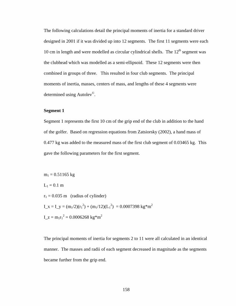
The following calculations detail the principal moments of inertia for a standard driver

designed in 2001 if it was divided up into 12 segments. The first 11 segments were each

10 cm in length and were modelled as circular cylindrical shells. The 12th segment was

the clubhead which was modelled as a semi-ellipsoid. These 12 segments were then

combined in groups of three. This resulted in four club segments. The principal

moments of inertia, masses, centers of mass, and lengths of these 4 segments were

determined using Autolev©.

Segment 1 Segment 1 represents the first 10 cm of the grip end of the club in addition to the hand

of the golfer. Based on regression equations from Zatsiorsky (2002), a hand mass of

0.477 kg was added to the measured mass of the first club segment of 0.03465 kg. This

gave the following parameters for the first segment.

m1 = 0.51165 kg

L1 = 0.1 m

r1 = 0.035 m (radius of cylinder)

I_x = I_y = (m1/2)(r12) + (m1/12)(L1

2) = 0.0007398 kg*m2

I_z = m1r12 = 0.0006268 kg*m2

The principal moments of inertia for segments 2 to 11 were all calculated in an identical

manner. The masses and radii of each segment decreased in magnitude as the segments

became further from the grip end.

158

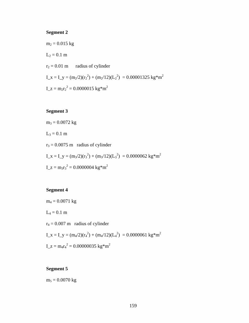
Segment 2

m2 = 0.015 kg

L2 = 0.1 m

r2 = 0.01 m radius of cylinder

I_x = I_y = (m2/2)(r22) + (m2/12)(L2

2) = 0.00001325 kg*m2

I_z = m2r22 = 0.0000015 kg*m2

Segment 3

m3 = 0.0072 kg

L3 = 0.1 m

r3 = 0.0075 m radius of cylinder

I_x = I_y = (m3/2)(r32) + (m3/12)(L3

2) = 0.0000062 kg*m2

I_z = m3r32 = 0.0000004 kg*m2

Segment 4

m4 = 0.0071 kg

L4 = 0.1 m

r4 = 0.007 m radius of cylinder

I_x = I_y = (m4/2)(r42) + (m4/12)(L4

2) = 0.0000061 kg*m2

I_z = m4r42 = 0.00000035 kg*m2

Segment 5

m5 = 0.0070 kg

159

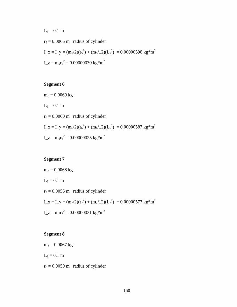
L5 = 0.1 m

r5 = 0.0065 m radius of cylinder

I_x = I_y = (m5/2)(r52) + (m5/12)(L5

2) = 0.00000598 kg*m2

I_z = m5r52 = 0.00000030 kg*m2

Segment 6

m6 = 0.0069 kg

L6 = 0.1 m

r6 = 0.0060 m radius of cylinder

I_x = I_y = (m6/2)(r62) + (m6/12)(L6

2) = 0.00000587 kg*m2

I_z = m6r62 = 0.00000025 kg*m2

Segment 7

m7 = 0.0068 kg

L7 = 0.1 m

r7 = 0.0055 m radius of cylinder

I_x = I_y = (m7/2)(r72) + (m7/12)(L7

2) = 0.00000577 kg*m2

I_z = m7r72 = 0.00000021 kg*m2

Segment 8

m8 = 0.0067 kg

L8 = 0.1 m

r8 = 0.0050 m radius of cylinder

160

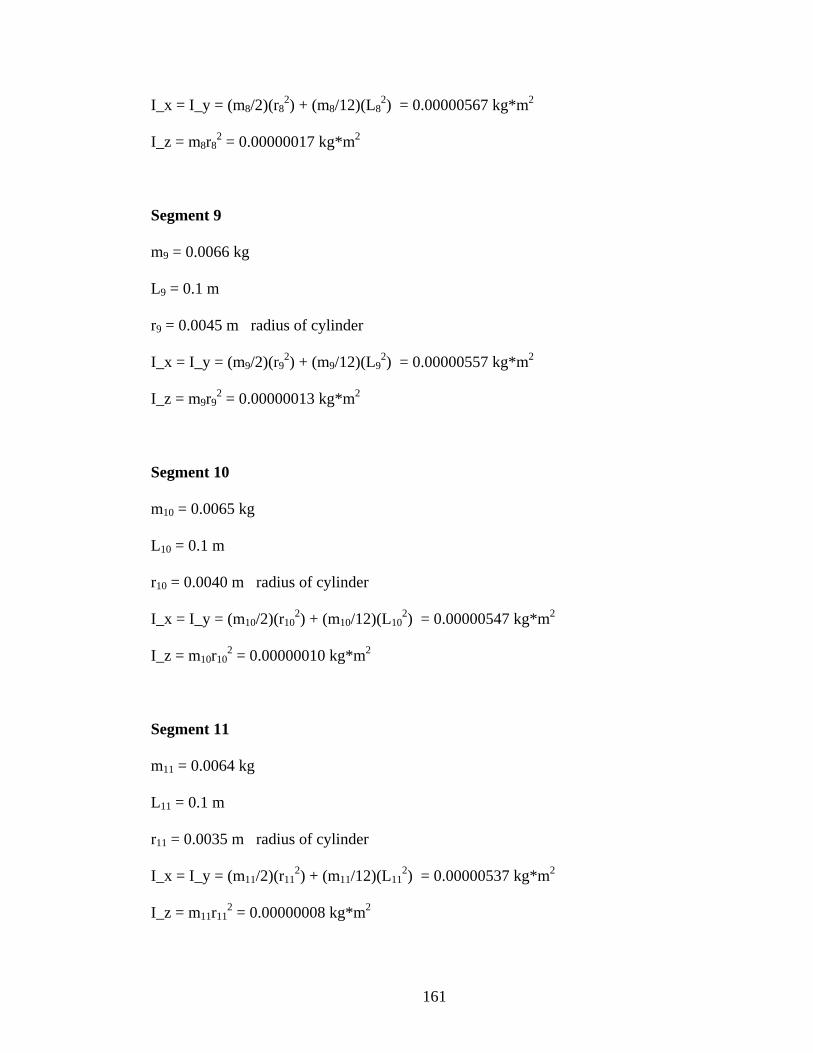
I_x = I_y = (m8/2)(r82) + (m8/12)(L8

2) = 0.00000567 kg*m2

I_z = m8r82 = 0.00000017 kg*m2

Segment 9

m9 = 0.0066 kg

L9 = 0.1 m

r9 = 0.0045 m radius of cylinder

I_x = I_y = (m9/2)(r92) + (m9/12)(L9

2) = 0.00000557 kg*m2

I_z = m9r92 = 0.00000013 kg*m2

Segment 10

m10 = 0.0065 kg

L10 = 0.1 m

r10 = 0.0040 m radius of cylinder

I_x = I_y = (m10/2)(r102) + (m10/12)(L10

2) = 0.00000547 kg*m2

I_z = m10r102 = 0.00000010 kg*m2

Segment 11

m11 = 0.0064 kg

L11 = 0.1 m

r11 = 0.0035 m radius of cylinder

I_x = I_y = (m11/2)(r112) + (m11/12)(L11

2) = 0.00000537 kg*m2

I_z = m11r112 = 0.00000008 kg*m2

161

Segment 12

Segment 12 represents the clubhead. The following equations are based on modelling

the clubhead as a semi-ellipsoid.

m12 = 0.2 kg

x = 0.11 m diameter of clubhead along the x-axis

y = 0.09 m diameter of clubhead along the y-axis

z = 0.05 m diameter of clubhead along the z-axis.

I_x = (m12/5)(z2 + (19/64)y2) = 0.000196 kg*m2

I_y = (m12/5)(z2 + x2) = 0.000584 kg*m2

I_z = (m12/5)(z2 + (19/64)y2) = 0.000580 kg*m2

The following is the Autolev© code that was used to generate the moments of inertia and

other parameter values for a 4 segment golf club based on the 12 segment club just

defined.

% shaftspecs.al % 12 SEGMENT PENDULUM . Sasho Mackenzie, NOVEMBER 15, 2004 % This program takes a 12 segment club and finds the corresponding % inertial parameters for a 6 segment, 4 segment, and 2 segment club. % This version has code for use in ANIMAKE % ------------------ %Physical declarations %Bodies refer to segments %Points refer to joint centres, with O fixed %(end of most distal or proximal seg) DEGREES ON AUTOZ ON NEWTONIAN N FRAMES B,D,F,H,J,L,O,Q,S,U,W BODIES A,C,E,G,I,K,M,P,R,T,V,X

162

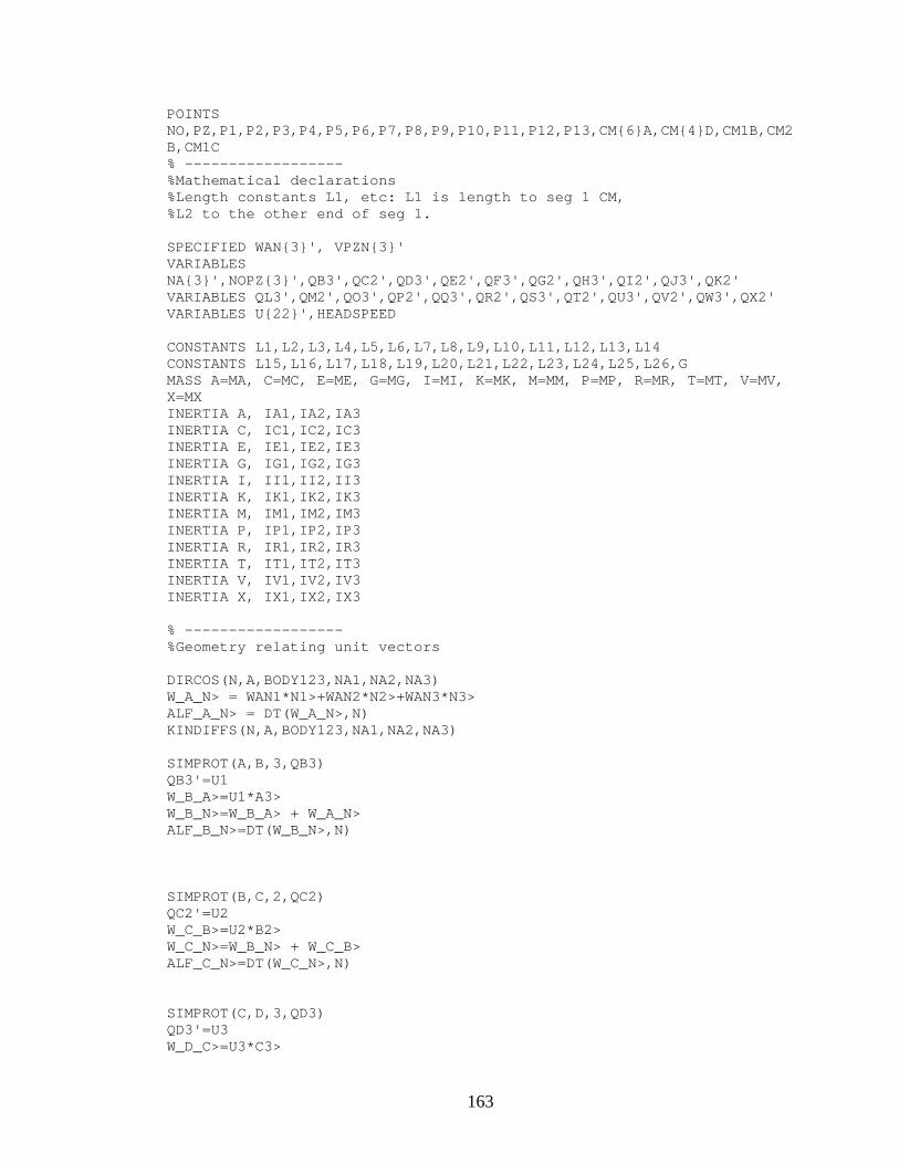
POINTS NO,PZ,P1,P2,P3,P4,P5,P6,P7,P8,P9,P10,P11,P12,P13,CM{6}A,CM{4}D,CM1B,CM2B,CM1C % ------------------ %Mathematical declarations %Length constants L1, etc: L1 is length to seg 1 CM, %L2 to the other end of seg 1. SPECIFIED WAN{3}', VPZN{3}' VARIABLES NA{3}',NOPZ{3}',QB3',QC2',QD3',QE2',QF3',QG2',QH3',QI2',QJ3',QK2' VARIABLES QL3',QM2',QO3',QP2',QQ3',QR2',QS3',QT2',QU3',QV2',QW3',QX2' VARIABLES U{22}',HEADSPEED CONSTANTS L1,L2,L3,L4,L5,L6,L7,L8,L9,L10,L11,L12,L13,L14 CONSTANTS L15,L16,L17,L18,L19,L20,L21,L22,L23,L24,L25,L26,G MASS A=MA, C=MC, E=ME, G=MG, I=MI, K=MK, M=MM, P=MP, R=MR, T=MT, V=MV, X=MX INERTIA A, IA1,IA2,IA3 INERTIA C, IC1,IC2,IC3 INERTIA E, IE1,IE2,IE3 INERTIA G, IG1,IG2,IG3 INERTIA I, II1,II2,II3 INERTIA K, IK1,IK2,IK3 INERTIA M, IM1,IM2,IM3 INERTIA P, IP1,IP2,IP3 INERTIA R, IR1,IR2,IR3 INERTIA T, IT1,IT2,IT3 INERTIA V, IV1,IV2,IV3 INERTIA X, IX1,IX2,IX3 % ------------------ %Geometry relating unit vectors DIRCOS(N,A,BODY123,NA1,NA2,NA3) W_A_N> = WAN1*N1>+WAN2*N2>+WAN3*N3> ALF_A_N> = DT(W_A_N>,N) KINDIFFS(N,A,BODY123,NA1,NA2,NA3) SIMPROT(A,B,3,QB3) QB3'=U1 W_B_A>=U1*A3> W_B_N>=W_B_A> + W_A_N> ALF_B_N>=DT(W_B_N>,N) SIMPROT(B,C,2,QC2) QC2'=U2 W_C_B>=U2*B2> W_C_N>=W_B_N> + W_C_B> ALF_C_N>=DT(W_C_N>,N) SIMPROT(C,D,3,QD3) QD3'=U3 W_D_C>=U3*C3>

163

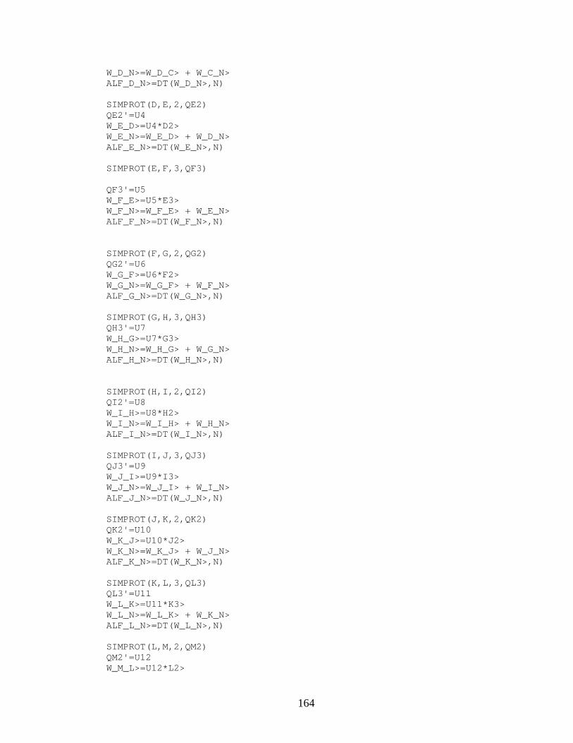
W_D_N>=W_D_C> + W_C_N> ALF_D_N>=DT(W_D_N>,N) SIMPROT(D,E,2,QE2) QE2'=U4 W_E_D>=U4*D2> W_E_N>=W_E_D> + W_D_N> ALF_E_N>=DT(W_E_N>,N) SIMPROT(E,F,3,QF3) QF3'=U5 W_F_E>=U5*E3> W_F_N>=W_F_E> + W_E_N> ALF_F_N>=DT(W_F_N>,N) SIMPROT(F,G,2,QG2) QG2'=U6 W_G_F>=U6*F2> W_G_N>=W_G_F> + W_F_N> ALF_G_N>=DT(W_G_N>,N) SIMPROT(G,H,3,QH3) QH3'=U7 W_H_G>=U7*G3> W_H_N>=W_H_G> + W_G_N> ALF_H_N>=DT(W_H_N>,N) SIMPROT(H,I,2,QI2) QI2'=U8 W_I_H>=U8*H2> W_I_N>=W_I_H> + W_H_N> ALF_I_N>=DT(W_I_N>,N) SIMPROT(I,J,3,QJ3) QJ3'=U9 W_J_I>=U9*I3> W_J_N>=W_J_I> + W_I_N> ALF_J_N>=DT(W_J_N>,N) SIMPROT(J,K,2,QK2) QK2'=U10 W_K_J>=U10*J2> W_K_N>=W_K_J> + W_J_N> ALF_K_N>=DT(W_K_N>,N) SIMPROT(K,L,3,QL3) QL3'=U11 W_L_K>=U11*K3> W_L_N>=W_L_K> + W_K_N> ALF_L_N>=DT(W_L_N>,N) SIMPROT(L,M,2,QM2) QM2'=U12 W_M_L>=U12*L2>

164

W_M_N>=W_M_L> + W_L_N> ALF_M_N>=DT(W_M_N>,N) SIMPROT(M,O,3,QO3) QO3'=U13 W_O_M>=U13*M3> W_O_N>=W_O_M> + W_M_N> ALF_O_N>=DT(W_O_N>,N) SIMPROT(O,P,2,QP2) QP2'=U14 W_P_O>=U14*O2> W_P_N>=W_P_O> + W_O_N> ALF_P_N>=DT(W_P_N>,N) SIMPROT(P,Q,3,QQ3) QQ3'=U15 W_Q_P>=U15*P3> W_Q_N>=W_Q_P> + W_P_N> ALF_Q_N>=DT(W_Q_N>,N) SIMPROT(Q,R,2,QR2) QR2'=U16 W_R_Q>=U16*Q2> W_R_N>=W_R_Q> + W_Q_N> ALF_R_N>=DT(W_R_N>,N) SIMPROT(R,S,3,QS3) QS3'=U17 W_S_R>=U17*R3> W_S_N>=W_S_R> + W_R_N> ALF_S_N>=DT(W_S_N>,N) SIMPROT(S,T,2,QT2) QT2'=U18 W_T_S>=U18*S2> W_T_N>=W_T_S> + W_S_N> ALF_T_N>=DT(W_T_N>,N) SIMPROT(T,U,3,QU3) QU3'=U19 W_U_T>=U19*T3> W_U_N>=W_U_T> + W_T_N> ALF_U_N>=DT(W_U_N>,N) SIMPROT(U,V,2,QV2) QV2'=U20 W_V_U>=U20*U2> W_V_N>=W_V_U> + W_U_N> ALF_V_N>=DT(W_V_N>,N) SIMPROT(V,W,3,QW3) QW3'=U21 W_W_V>=U21*V3> W_W_N>=W_W_V> + W_V_N> ALF_W_N>=DT(W_W_N>,N)

165

SIMPROT(W,X,2,QX2) QX2'=U22 W_X_W>=U22*X2> W_X_N>=W_X_W> + W_W_N> ALF_X_N>=DT(W_X_N>,N) % ------------------ %Position Vectors %use lengths and Local Co-ord Sys (LCS) to define P_NO_PZ>=NOPZ1*N1> + NOPZ2*N2> + NOPZ3*N3> V_PZ_N>=VPZN1*N1> + VPZN2*N2> + VPZN3*N3> NOPZ1'=VPZN1 NOPZ2'=VPZN2 NOPZ3'=VPZN3 A_PZ_N>=DT(V_PZ_N>,N) P_PZ_AO>=L1*A1> P_AO_P1>=(L2-L1)*A1> P_P1_CO>=L3*C1> P_P1_P2>=L4*C1> P_P2_EO>=L5*E1> P_P2_P3>=L6*E1> P_P3_GO>=L7*G1> P_P3_P4>=L8*G1> P_P4_IO>=L9*I1> P_P4_P5>=L10*I1> P_P5_KO>=L11*K1> P_P5_P6>=L12*K1> P_P6_MO>=L13*M1> P_P6_P7>=L14*M1> P_P7_PO>=L15*P1> P_P7_P8>=L16*P1> P_P8_RO>=L17*R1> P_P8_P9>=L18*R1> P_P9_TO>=L19*T1> P_P9_P10>=L20*T1> P_P10_VO>=L21*V1> P_P10_P11>=L22*V1> P_P11_XO>=L23*X1>-L24*X2>-L25*X3> P_P11_P12>=L26*X1> P_P12_P13>=-L24*X2>-L25*X3> %use vector addition to define 2nd seg points relative to origin P_NO_AO>=P_NO_PZ> + P_PZ_AO> P_NO_P1>=P_NO_AO> + P_AO_P1> P_NO_CO>=P_NO_P1>+P_P1_CO> P_NO_P2>=P_NO_P1>+P_P1_P2> P_NO_EO>=P_NO_P2>+P_P2_EO> P_NO_P3>=P_NO_P2>+P_P2_P3> P_NO_GO>=P_NO_P3>+P_P3_GO>

166

P_NO_P4>=P_NO_P3>+P_P3_P4> P_NO_IO>=P_NO_P4>+P_P4_IO> P_NO_P5>=P_NO_P4>+P_P4_P5> P_NO_KO>=P_NO_P5>+P_P5_KO> P_NO_P6>=P_NO_P5>+P_P5_P6> P_NO_MO>=P_NO_P6>+P_P6_MO> P_NO_P7>=P_NO_P6>+P_P6_P7> P_NO_PO>=P_NO_P7>+P_P7_PO> P_NO_P8>=P_NO_P7>+P_P7_P8> P_NO_RO>=P_NO_P8>+P_P8_RO> P_NO_P9>=P_NO_P8>+P_P8_P9> P_NO_TO>=P_NO_P9>+P_P9_TO> P_NO_P10>=P_NO_P9>+P_P9_P10> P_NO_VO>=P_NO_P10>+P_P10_VO> P_NO_P11>=P_NO_P10>+P_P10_P11> P_NO_XO>=P_NO_P11>+P_P11_XO> P_NO_P12>=P_NO_P11>+P_P11_P12> P_NO_P13>=P_NO_P12>+P_P12_P13> NA1=0 NA2=0 NA3=0 NOPZ1=-0.1881 NOPZ2=0.3168 NOPZ3=0.0 L1=.05 L2=.1 L3=.05 L4=.1 L5=.05 L6=.1 L7=.05 L8=.1 L9=.05 L10=.1 L11=.05 L12=.1 L13=.05 L14=.1 L15=.05 L16=.1 L17=.05 L18=.1 L19=.05 L20=.1 L21=.05 L22=.1 L23=0.025 L24=0.055 L25=0.05 L26=0.025 IA1=0.0006268 IA2=0.0007398 IA3=0.0007398 IC1=0.0000015 IC2=0.00001325 IC3=0.00001325

167

IE1=0.0000004 IE2=0.0000062 IE3=0.0000062 IG1=0.00000035 IG2=0.0000061 IG3=0.0000061 II1=0.0000003 II2=0.00000598 II3=0.00000598 IK1=0.00000025 IK2=0.00000587 IK3=0.00000587 IM1=0.00000021 IM2=0.00000577 IM3=0.00000577 IP1=0.00000017 IP2=0.00000567 IP3=0.00000567 IR1=0.00000013 IR2=0.00000557 IR3=0.00000557 IT1=0.0000001 IT2=0.00000547 IT3=0.00000547 IV1=0.00000008 IV2=0.00000537 IV3=0.00000537 IX1=0.000580 IX2=0.000196 IX3=0.000584 MA=0.51165 MC=0.015 ME=0.0072 MG=0.0071 MI=0.0070 MK=0.0069 MM=0.0068 MP=0.0067 MR=0.0066 MT=0.0065 MV=0.0064 MX=0.2 QB3=0 QC2=0 QD3=0 QE2=0 QF3=0 QG2=0 QH3=0 QI2=0 QJ3=0 QK2=0 QL3=0 QM2=0 QO3=0 QP2=0 QQ3=0

168

QR2=0 QS3=0 QT2=0 QU3=0 QV2=0 QW3=0 QX2=0 UNITS [L1,L2,L3,L4,L5,L6,L7,L8,L9,L10]=M UNITS NA{1:3}=DEG UNITS [QB3,QC2,QD3,QE2,QF3,QG2,QH3,QI2,QJ3,QK2,QL3,QM2,QO3,QP2,QQ3,QR2,QS3,QT2,QU3,QV2,QW3,QX2]=DEG UNITS NOPZ{1:3}=M UNITS [IA1,IA2,IA3,IC1,IC2,IC3,IE1,IE2,IE3,IG1,IG2,IG3]=KG*M^2 UNITS [MA,MC,ME,MG]=KG % FINDING THE SPECS FOR A 6 SEGMENT CLUB: REFERRED TO AS 'A' P_PZ_CM1A>=EXPLICIT(CM(PZ,A,C)) P_P2_CM2A>=EXPLICIT(CM(P2,E,G)) P_P4_CM3A>=EXPLICIT(CM(P4,I,K)) P_P6_CM4A>=EXPLICIT(CM(P6,M,P)) P_P8_CM5A>=EXPLICIT(CM(P8,R,T)) P_P10_CM6A>=EXPLICIT(CM(P10,V,X)) L1NEWA=EXPLICIT(MAG(P_PZ_CM1A>)) L3NEWA=EXPLICIT(MAG(P_P2_CM2A>)) L5NEWA=EXPLICIT(MAG(P_P4_CM3A>)) L7NEWA=EXPLICIT(MAG(P_P6_CM4A>)) L9NEWA=EXPLICIT(MAG(P_P8_CM5A>)) L11NEWA=EXPLICIT(MAG(P_P10_CM6A>)) I_A_AND_C_CM1A>>=INERTIA(CM1A,A,C) I_E_AND_G_CM2A>>=INERTIA(CM2A,E,G) I_I_AND_K_CM3A>>=INERTIA(CM3A,I,K) I_M_AND_P_CM4A>>=INERTIA(CM4A,M,P) I_R_AND_T_CM5A>>=INERTIA(CM5A,R,T) I_V_AND_X_CM6A>>=INERTIA(CM6A,V,X) I_ANEWA_CM1A=EXPLICIT(REPRESENT(I_A_AND_C_CM1A>>,A)) I_CNEWA_CM2A=EXPLICIT(REPRESENT(I_E_AND_G_CM2A>>,E)) I_ENEWA_CM3A=EXPLICIT(REPRESENT(I_I_AND_K_CM3A>>,I)) I_GNEWA_CM4A=EXPLICIT(REPRESENT(I_M_AND_P_CM4A>>,M)) I_INEWA_CM5A=EXPLICIT(REPRESENT(I_R_AND_T_CM5A>>,R)) I_KNEWA_CM6A=EXPLICIT(REPRESENT(I_V_AND_X_CM6A>>,V)) I_ANEWA=EIG(I_ANEWA_CM1A) I_CNEWA=EIG(I_CNEWA_CM2A) I_ENEWA=EIG(I_ENEWA_CM3A) I_GNEWA=EIG(I_GNEWA_CM4A) I_INEWA=EIG(I_INEWA_CM5A) I_KNEWA=EIG(I_KNEWA_CM6A) MANEWA=MA+MC MCNEWA=ME+MG MENEWA=MI+MK

169

MGNEWA=MM+MP MINEWA=MR+MT MKNEWA=MV+MX % FINDING THE SPECS FOR A 4 SEGMENT CLUB: REFERRED TO AS 'D' P_PZ_CM1D>=EXPLICIT(CM(PZ,A,C,E)) P_P3_CM2D>=EXPLICIT(CM(P3,G,I,K)) P_P6_CM3D>=EXPLICIT(CM(P6,M,P,R)) P_P9_CM4D>=EXPLICIT(CM(P9,T,V,X)) L1NEWD=EXPLICIT(MAG(P_PZ_CM1D>)) L3NEWD=EXPLICIT(MAG(P_P3_CM2D>)) L5NEWD=EXPLICIT(MAG(P_P6_CM3D>)) L7NEWD=EXPLICIT(MAG(P_P9_CM4D>)) I_A_TO_E_CM1D>>=INERTIA(CM1D,A,C,E) I_G_TO_K_CM2D>>=INERTIA(CM2D,G,I,K) I_M_TO_R_CM3D>>=INERTIA(CM3D,M,P,R) I_T_TO_X_CM4D>>=INERTIA(CM4D,T,V,X) I_ANEWD_CM1D=EXPLICIT(REPRESENT(I_A_TO_E_CM1D>>,A)) I_CNEWD_CM2D=EXPLICIT(REPRESENT(I_G_TO_K_CM2D>>,G)) I_ENEWD_CM3D=EXPLICIT(REPRESENT(I_M_TO_R_CM3D>>,M)) I_GNEWD_CM4D=EXPLICIT(REPRESENT(I_T_TO_X_CM4D>>,T)) I_ANEWD=EIG(I_ANEWD_CM1D) I_CNEWD=EIG(I_CNEWD_CM2D) I_ENEWD=EIG(I_ENEWD_CM3D) I_GNEWD=EIG(I_GNEWD_CM4D) MANEWD=MA+MC+ME MCNEWD=MG+MI+MK MENEWD=MM+MP+MR MGNEWD=MT+MV+MX % FINDING THE SPECS FOR A 2 SEGMENT CLUB: REFERRED TO AS 'B' P_PZ_CM1B>=EXPLICIT(CM(PZ,A,C,E,G,I,K)) P_P6_CM2B>=EXPLICIT(CM(P6,M,P,R,T,V,X)) L1NEWB=EXPLICIT(MAG(P_PZ_CM1B>)) L3NEWB=EXPLICIT(MAG(P_P6_CM2B>)) I_A_TO_K_CM1B>>=INERTIA(CM1B,A,C,E,G,I,K) I_M_TO_X_CM2B>>=INERTIA(CM2B,M,P,R,T,V,X) I_ANEWB_CM1B=EXPLICIT(REPRESENT(I_A_TO_K_CM1B>>,A)) I_CNEWB_CM2B=EXPLICIT(REPRESENT(I_M_TO_X_CM2B>>,M)) I_ANEWB=EIG(I_ANEWB_CM1B) I_CNEWB=EIG(I_CNEWB_CM2B)

170

MANEWB=MA+MC+ME+MG+MI+MK MCNEWB=MM+MP+MR+MT+MV+MX % FINDING THE SPECS FOR A 1 SEGMENT CLUB: REFERRED TO AS 'C' %P_PZ_CM1C>=EXPLICIT(CM(PZ,A,C,E,G,I,K,M,P,R,T,V,X)) %L1NEWC=EXPLICIT(MAG(P_PZ_CM1C>)) %I_A_TO_X_CM1C>>=INERTIA(CM1C,A,C,E,G,I,K,M,P,R,T,V,X) %I_ANEWC_CM1C=EXPLICIT(REPRESENT(I_A_TO_X_CM1C>>,A)) %I_ANEWC=EIG(I_ANEWC_CM1C) %MANEWC=MA+MC+ME+MG+MI+MK+MM+MP+MR+MT+MV+MX SAVE SHAFTSPECS.ALL

171

APPENDIX C

Autolev© Code: 3DGOLFG.AL

172

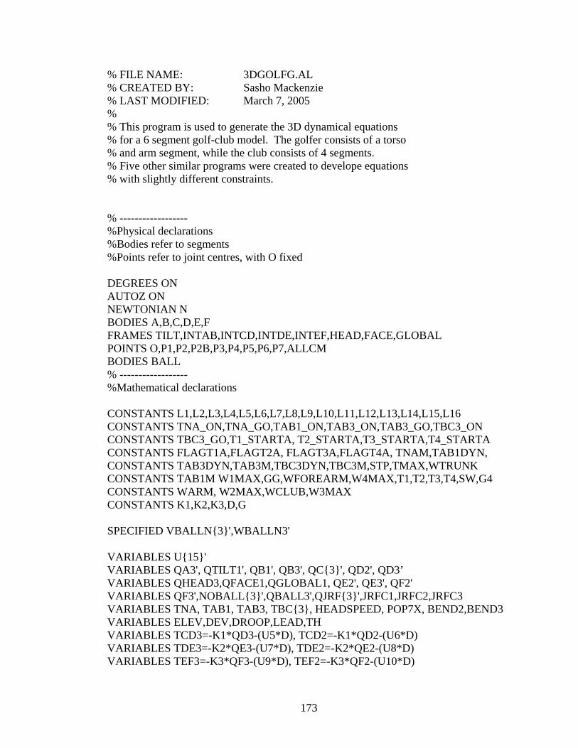
% FILE NAME: 3DGOLFG.AL % CREATED BY: Sasho Mackenzie % LAST MODIFIED: March 7, 2005 % % This program is used to generate the 3D dynamical equations % for a 6 segment golf-club model. The golfer consists of a torso % and arm segment, while the club consists of 4 segments. % Five other similar programs were created to develope equations % with slightly different constraints. % ------------------ %Physical declarations %Bodies refer to segments %Points refer to joint centres, with O fixed DEGREES ON AUTOZ ON NEWTONIAN N BODIES A,B,C,D,E,F FRAMES TILT,INTAB,INTCD,INTDE,INTEF,HEAD,FACE,GLOBAL POINTS O,P1,P2,P2B,P3,P4,P5,P6,P7,ALLCM BODIES BALL % ------------------ %Mathematical declarations CONSTANTS L1,L2,L3,L4,L5,L6,L7,L8,L9,L10,L11,L12,L13,L14,L15,L16 CONSTANTS TNA_ON,TNA_GO,TAB1_ON,TAB3_ON,TAB3_GO,TBC3_ON CONSTANTS TBC3_GO,T1_STARTA, T2_STARTA,T3_STARTA,T4_STARTA CONSTANTS FLAGT1A,FLAGT2A, FLAGT3A,FLAGT4A, TNAM,TAB1DYN, CONSTANTS TAB3DYN,TAB3M,TBC3DYN,TBC3M,STP,TMAX,WTRUNK CONSTANTS TAB1M W1MAX,GG,WFOREARM,W4MAX,T1,T2,T3,T4,SW,G4 CONSTANTS WARM, W2MAX,WCLUB,W3MAX CONSTANTS K1,K2,K3,D,G SPECIFIED VBALLN{3}',WBALLN3' VARIABLES U{15}' VARIABLES QA3', QTILT1', QB1', QB3', QC{3}', QD2', QD3’ VARIABLES QHEAD3,QFACE1,QGLOBAL1, QE2', QE3', QF2' VARIABLES QF3',NOBALL{3}',QBALL3',QJRF{3}',JRFC1,JRFC2,JRFC3 VARIABLES TNA, TAB1, TAB3, TBC{3}, HEADSPEED, POP7X, BEND2,BEND3 VARIABLES ELEV,DEV,DROOP,LEAD,TH VARIABLES TCD3=-K1*QD3-(U5*D), TCD2=-K1*QD2-(U6*D) VARIABLES TDE3=-K2*QE3-(U7*D), TDE2=-K2*QE2-(U8*D) VARIABLES TEF3=-K3*QF3-(U9*D), TEF2=-K3*QF2-(U10*D)

173

VARIABLES X1,X2,X3,X4,X5,Y1,Y2,Y3,Y4,Y5,TH1,TH2,TH3,TH4,TORK1 VARIABLES TORK2,TORK3 ZEE_NOT = [TBC1,TBC2,JRFC1,JRFC2,JRFC3] MASS A=MA, B=MB, C=MC, D=MD, E=ME, F=MF, BALL=MBALL INERTIA A, IA1,IA2,IA3 INERTIA B, IB1,IB2,IB3 INERTIA C, IC1,IC2,IC3 INERTIA D, ID1,ID2,ID3 INERTIA E, IE1,IE2,IE3 INERTIA F, IF1,IF2,IF3 INERTIA BALL,IBALL3,IBALL3,IBALL3 % ------------------ %Geometry relating unit vectors SIMPROT(N,A,3,QA3) SIMPROT(N,TILT,1,QTILT1) SIMPROT(TILT,INTAB,3,QB3) SIMPROT(INTAB,B,1,QB1) DIRCOS(B,C,BODY123,QC1,QC2,QC3) SIMPROT(C,INTCD,3,QD3) SIMPROT(INTCD,D,2,QD2) SIMPROT(D,INTDE,3,QE3) SIMPROT(INTDE,E,2,QE2) SIMPROT(E,INTEF,3,QF3) SIMPROT(INTEF,F,2,QF2) SIMPROT(F,HEAD,3,QHEAD3) SIMPROT(HEAD,FACE,FACE1>,QFACE1) SIMPROT(N,GLOBAL,1,QGLOBAL1) %__________________________________________________ %FOR THE FLIGHT OF THE BALL P_O_BALLO>=NOBALL1*N1>+NOBALL2*N2>+NOBALL3*N3> V_BALLO_N>=VBALLN1*N1>+VBALLN2*N2>+VBALLN3*N3> NOBALL1'=VBALLN1 NOBALL2'=VBALLN2 NOBALL3'=VBALLN3 A_BALLO_N>=DT(V_BALLO_N>,N) SIMPROT(N,BALL,3,QBALL3) QBALL3'=WBALLN3 W_BALL_N>=WBALLN3*N3> ALF_BALL_N>=DT(W_BALL_N>,N)

174

% ------------------ %Position Vectors %use lengths and Local Co-ord Sys (LCS) to define P_O_AO>=L1*A1> P_O_P1>=L2*A1> P_P1_BO>=L3*B1> P_P1_P2>=L4*B1> P_P2_P2B>= QJRF1*N1> + QJRF2*N2> + QJRF3*N3> P_P2B_CO>=L5*C1> P_P2B_P3>=L6*C1> P_P3_DO>=L7*D1> P_P3_P4>=L8*D1> P_P4_EO>=L9*E1> P_P4_P5>=L10*E1> P_P5_FO>=L11*F1>-L13*F2>-L14*F3> P_P5_P6>=L12*F1> P_P6_P7>=-L15*F2>-L16*F3> P_P7_HEADO>=0> P_HEADO_FACEO>=0> P_O_GLOBALO>=0> P_O_TILTO>=0> P_P1_INTABO>=0> P_P3_INTCDO>=0> P_P4_INTDEO>=0> P_P5_INTEFO>=0> %use vector addition to define 2nd seg points relative to origin P_O_BO>=P_O_P1>+P_P1_BO> P_O_P2>=P_O_P1>+P_P1_P2> P_O_P2B>=P_O_P2> + P_P2_P2B> P_O_CO>=P_O_P2B>+P_P2B_CO> P_O_P3>=P_O_P2B>+P_P2B_P3> P_O_DO>=P_O_P3>+P_P3_DO> P_O_P4>=P_O_P3>+P_P3_P4> P_O_EO>=P_O_P4>+P_P4_EO> P_O_P5>=P_O_P4>+P_P4_P5> P_O_FO>=P_O_P5>+P_P5_FO> P_O_P6>=P_O_P5>+P_P5_P6> P_O_P7>=P_O_P6>+P_P6_P7>

175

P_O_HEADO>=P_O_P7>+P_P7_HEADO> P_O_FACEO>=P_O_HEADO>+P_HEADO_FACEO> P_O_INTABO>=P_O_P1>+P_P1_INTABO> P_O_INTCDO>=P_O_P3>+P_P3_INTCDO> P_O_INTDEO>=P_O_P4>+P_P4_INTDEO> P_O_INTEFO>=P_O_P5>+P_P5_INTEFO> % Implementing torques TORQUE(N/A,TNA*N3>) TORQUE(A/B,TAB3*TILT3>) %TORQUE(A/B,TAB3*A3>) % TORQUE(A/B,TAB1*INTAB1>) TORQUE(B/C,TBC3*C3>) TORQUE(B/C,TBC2*C2>) TORQUE(B/C,TBC1*C1>) % Implementing spring torques TORQUE(C/INTCD,TCD3*C3>) TORQUE(INTCD/D,TCD2*INTCD2>) TORQUE(D/INTDE,TDE3*D3>) TORQUE(INTDE/E,TDE2*INTDE2>) TORQUE(E/INTEF,TEF3*E3>) TORQUE(INTEF/F,TEF2*INTEF2>) % Implementing the forces acting on the grip end of the club FORCE(P2/P2B, JRFC1*C1> + JRFC2*C2> + JRFC3*C3>) % ------------------ % The following commands are for ANIMAKE ANIMATE(N,O,A,B,C,D,E,F,BALL,TILT,INTAB,INTCD,INTDE,INTEF,HEAD,FACE,GLOBAL) % -------------------- %X and Y positions of joints %use vector dot products to get x,y coords. of joints %needed for MatLab plotting program SimPlotAL POP1X=DOT(P_O_P1>,N1>) POP1Y=DOT(P_O_P1>,N2>) POP2X=DOT(P_O_P2>,N1>) POP2Y=DOT(P_O_P2>,N2>) POP3X=DOT(P_O_P3>,N1>) POP3Y=DOT(P_O_P3>,N2>) POP4X=DOT(P_O_P4>,N1>) POP4Y=DOT(P_O_P4>,N2>) POP5X=DOT(P_O_P5>,N1>) POP5Y=DOT(P_O_P5>,N2>) POP7X=DOT(P_O_P7>,N1>)

176

POP7Y=DOT(P_O_P7>,GLOBAL3>) % ------------------ % Determing the coordinates of the shaft in the plane of the swing X1=DOT(P_O_P2>,INTAB1>) Y1=DOT(P_O_P2>,INTAB2>) X2=DOT(P_O_P3>,INTAB1>) Y2=DOT(P_O_P3>,INTAB2>) X3=DOT(P_O_P4>,INTAB1>) Y3=DOT(P_O_P4>,INTAB2>) X4=DOT(P_O_P5>,INTAB1>) Y4=DOT(P_O_P5>,INTAB2>) X5=DOT(P_O_P6>,INTAB1>) Y5=DOT(P_O_P6>,INTAB2>) % Determining the shaft bending angle in the plane of the swing TH1= ATAN( ABS(X1-X2) / ABS(Y1-Y2) ) TH2= ATAN( ABS(X2-X3) / ABS(Y2-Y3) ) TH3= ATAN( ABS(X3-X4) / ABS(Y3-Y4) ) TH4= ATAN( ABS(X4-X5) / ABS(Y4-Y5) ) % ------------------ %Angular velocities & accelerations W_A_N> =U1*N3> W_TILT_N> =0> W_INTAB_TILT> =U2*TILT3> W_INTAB_N> =W_INTAB_TILT> + W_TILT_N> W_B_INTAB> =U3*INTAB1> W_B_N> =W_B_INTAB> + W_INTAB_N> W_C_B> =U11*C1> + U12*C2> + U4*C3> W_C_N> =W_C_B> + W_B_N> W_INTCD_C> =U5*C3> W_INTCD_N> =W_INTCD_C> + W_C_N> W_D_INTCD> =U6*INTCD2> W_D_N> =W_D_INTCD> + W_INTCD_N> W_INTDE_D> =U7*D3> W_INTDE_N> =W_INTDE_D> + W_D_N>

177

W_E_INTDE> =U8*INTDE2> W_E_N> =W_E_INTDE> + W_INTDE_N> W_INTEF_E> =U9*E3> W_INTEF_N> =W_INTEF_E> + W_E_N> W_F_INTEF> =U10*INTEF2> W_F_N> =W_F_INTEF> + W_INTEF_N> OMEGXC = DOT(W_C_N>,N1>) OMEGYC = DOT(W_C_N>,N2>) OMEGZC = DOT(W_C_N>,N3>) % ALF_A_N>=DT(W_A_N>,N) ALF_B_N>=DT(W_B_N>,N) ALF_C_N>=DT(W_C_N>,N) ALF_D_N>=DT(W_D_N>,N) ALF_E_N>=DT(W_E_N>,N) ALF_F_N>=DT(W_F_N>,N) ALPHXC = DOT(ALF_C_N>,N1>) ALPHYC = DOT(ALF_C_N>,N2>) ALPHZC = DOT(ALF_C_N>,N3>) % ------------------ %Kinematical differential equations QA3'=U1 QB3'=U2 QB1'=U3 KINDIFFS(B,C,BODY123,QC1,QC2,QC3) QD3'=U5 QD2'=U6 QE3'=U7 QE2'=U8 QF3'=U9 QF2'=U10 QJRF1'=U13 QJRF2'=U14 QJRF3'=U15

178

%Linear velocities & accelerations %V_O_N>=0> V_AO_N>=DT(P_O_AO>,N) V_P1_N>=DT(P_O_P1>,N) V_BO_N>=DT(P_O_BO>,N) V_P2_N>=DT(P_O_P2>,N) V_CO_N>=DT(P_O_CO>,N) V_P3_N>=DT(P_O_P3>,N) V_DO_N>=DT(P_O_DO>,N) V_P4_N>=DT(P_O_P4>,N) V_EO_N>=DT(P_O_EO>,N) V_P5_N>=DT(P_O_P5>,N) V_FO_N>=DT(P_O_FO>,N) V_P6_N>=DT(P_O_P6>,N) V_P7_N>=DT(P_O_P7>,N) HEADSPEED = DOT(V_P7_N>,N1>) V_P2B_N> = V_P2_N> + U13*N1> + U14*N2> + U15*N3> VELP2X = DOT(V_P2_N>,N1>) VELP2Y = DOT(V_P2_N>,N2>) VELP2Z = DOT(V_P2_N>,N3>) VELXC = DOT(V_CO_N>,N1>) VELYC = DOT(V_CO_N>,N2>) VELZC = DOT(V_CO_N>,N3>) % A_O_N>=0> A_AO_N>=DT(V_AO_N>,N) A_P1_N>=DT(V_P1_N>,N) A_BO_N>=DT(V_BO_N>,N) A_P2_N>=DT(V_P2_N>,N) A_CO_N>=DT(V_CO_N>,N) A_P3_N>=DT(V_P3_N>,N) A_DO_N>=DT(V_DO_N>,N) A_P4_N>=DT(V_P4_N>,N) A_EO_N>=DT(V_EO_N>,N) A_P5_N>=DT(V_P5_N>,N) A_FO_N>=DT(V_FO_N>,N) A_P6_N>=DT(V_P6_N>,N) A_P7_N>=DT(V_P7_N>,N) A_P2B_N>=DT(V_P2B_N>,N)

179

%AYA = DOT(A_P2_N>,B2>) HEADACCEL = DOT(A_P7_N>,N1>) ACCELP2X = DOT(A_P2_N>,N1>) ACCELP2Y = DOT(A_P2_N>,N2>) ACCELP2Z = DOT(A_P2_N>,N3>) BEND2 = QD2+QE2+QF2 BEND3 = QD3+QE3+QF3 % Applying motion constraints to the system %AUXILIARY=[U2-U1;U3;U4;U11;U12;U13;U14;U15] AUXILIARY=[U11;U12;U13;U14;U15] %DEPENDENT= [U5;U6] %CONSTRAIN(AUXILIARY[U2,U3,U4,U11,U12,U13,U14,U15]) CONSTRAIN(AUXILIARY[U11,U12,U13,U14,U15]) % ------------------ %Forces %TORSO OF GOLFER IS INCLINED RELATIVE TO THE VERTICAL GRAVITY(SIN(30)*G*N2> + SIN(60)*G*N3>) %USE THE NUMERICAL INTEGRATION CHECKING FUNCTION CHECK = NICHECK() %----------------------------------------------------- % DETERMINE CM LOCATION, KE AND PE FOR ALL % P_O_ALLCM> = CM(O) HTALL = DOT(P_O_ALLCM>,N2>) KEALL = KE() PEALL = -1*RHS(HTALL)*(MA+MB+MC+MD+ME+MF)*G % -G as on input G=-9.81 TEALL = RHS(KEALL)+RHS(PEALL) % %use vector dot products to get x, y and z component of acceleration % ACCELXD=DOT(A_DO_N>,N1>) ACCELYD=DOT(A_DO_N>,N2>) ACCELZD=DOT(A_DO_N>,N3>) JFXD=MD*ACCELXD JFYD=MD*ACCELYD - MD*SIN(30)*G JFZD=MD*ACCELZD - MD*SIN(60)*G ACCELXC=DOT(A_CO_N>,N1>)

180

ACCELYC=DOT(A_CO_N>,N2>) ACCELZC=DOT(A_CO_N>,N3>) JFXC=MC*ACCELXC + JFXD JFYC=MC*ACCELYC - MC*SIN(30)*G + JFYD JFZC=MC*ACCELZC - MC*SIN(60)*G + JFZD % ------------------ %Equations of motion ZERO = FR() + FRSTAR() %KANE(TAB3,TAB1,TBC3) KANE(TBC1,TBC2,JRFC1,JRFC2,JRFC3) % Calculating the direction the clubface is pointing ELEV = PI/2 - ACOS(DOT(GLOBAL2>,FACE3>)) DEV = PI/2 - ACOS(DOT(GLOBAL3>,FACE3>)) % Calculating the displacement of the clubhead relative to the grip end DROOP = DOT((P_O_P2>-P_O_P6>),C2>) LEAD = DOT((P_O_P2>-P_O_P6>),C3>) % Calculating the torques AND forces acting on the gripend of the club relative to N> TORK1=DOT(TBC1*C1> + TBC2*C2> + TBC3*C3>,N1>) TORK2=DOT(TBC1*C1> + TBC2*C2> + TBC3*C3>,N2>) TORK3=DOT(TBC1*C1> + TBC2*C2> + TBC3*C3>,N3>) FORC1=DOT(JRFC1*C1> + JRFC2*C2> + JRFC3*C3>,N1>) FORC2=DOT(JRFC1*C1> + JRFC2*C2> + JRFC3*C3>,N2>) FORC3=DOT(JRFC1*C1> + JRFC2*C2> + JRFC3*C3>,N3>) % ------------------ %Inputs INPUT TINITIAL=0.0, TFINAL=0.4, INTEGSTP=0.001, PRINTINT=1 INPUT ABSERR=1.0E-05, RELERR=1.0E-04 INPUT TNA = 0.0, K1=350,K2=325,K3=300, TAB3 = 0.0 , TAB1 = 0.0, TBC3 = 0.0 INPUT [QB1,QD2,QD3,QE2,QE3,QF2,QF3]=0.0, QA3=270, QTILT1=15, QB3=110, QC3=-110,QHEAD3=-45,QFACE1=10,QGLOBAL1=60 % Inertial paramenters are taken from Zatsiorsky (2002), Kinetics of Human Motion p.591 % Values are based on an 80 kg man with segment lengths the same as mine. See Bodyspecs.al and shaftspecs.al INPUT L1=0.0, L2=0.2, L3=0.2613, L4=0.6 INPUT L5=.05550716,L7=.1490476,L9=.149005,L11=.2174025 INPUT L12=.225,L13=.05166745,L14=.04697041,L15=.055,L16=.05,[L6,L8,L10]=0.3 INPUT IA1=0.17256,IA2=0.07052,IA3=0.36552 INPUT IB1=0.005806,IB2=0.1076,IB3=0.1096

181

INPUT IC1=0.0006287, [IC2,IC3]=0.001181059 INPUT ID1=0.0000009, [ID2,ID3]=0.000157931 INPUT IE1=0.00000051, [IE2,IE3]=0.0001509901 INPUT IF1=0.0004199793, IF2=0.0006621033,IF3=0.0008792326 INPUT MA=34.613, MB=3.431 INPUT MC=0.53385, MD=0.021, ME=0.0201, MF=0.2129, MBALL=0.04569 INPUT G=-9.81 INPUT D=10 INPUT U1=-5 INPUT IBALL3=0.0001 INPUT NOBALL1=0.29,NOBALL2=-1.71,NOBALL3=0.203 INPUT [TNA_ON,TNA_GO,TAB1_ON,TAB3_ON,TAB3_GO,TBC3_ON,TBC3_GO,T1_STARTA]=0 INPUT [T2_STARTA,T3_STARTA,T4_STARTA,FLAGT1A,FLAGT2A,FLAGT3A,FLAGT4A]=0 INPUT [TNAM,TAB1DYN,TAB1M,TAB3DYN,TAB3M,TBC3DYN,TBC3M,STP,TMAX,WTRUNK]=0 INPUT [W1MAX,GG,WFOREARM,W4MAX,T1,T2,T3,T4]=0 INPUT [SW,G4,WARM,W2MAX,WCLUB,W3MAX]=0 % ------------------ %Outputs %each line defines output file FILENAME.1,FILENAME.2,etc. %FILENAME.1 is needed for MatLab plotting program SimPlotAL %FILENAME.2 is 'standard' AutoLev output file with angular kinematics OUTPUT T, TNA, TAB1, TAB3, TBC3, TCD2, TCD3, HEADSPEED, POP7X,POP7Y,CHECK,HEADACCEL OUTPUT T, QA3, U1, QB3, U2, QB1, U3, QC3, U4, QD3, U5, QD2, U6, QE3,U7,QE2,U8,QF3,U9,QF2,U10,TH,BEND2, BEND3 OUTPUT T, ELEV, DEV, DROOP, LEAD OUTPUT T, OMEGXC, OMEGYC, OMEGZC, VELP2X, VELP2Y, VELP2Z OUTPUT T, ALPHXC, ALPHYC, ALPHZC, ACCELP2X, ACCELP2Y, ACCELP2Z OUTPUT T, TBC1,TBC2,TBC3,TORK1,TORK2,TORK3,JRFC1,JRFC2,JRFC3,FORC1,FORC2,FORC3 OUTPUT TNA_ON,TNA_GO,TAB1_ON,TAB3_ON,TAB3_GO,TBC3_ON,TBC3_GO,T1_STARTA OUTPUT T2_STARTA,T3_STARTA,T4_STARTA,FLAGT1A,FLAGT2A,FLAGT3A,FLAGT4A

182

OUTPUT TNAM,TAB1DYN,TAB1M,TAB3DYN,TAB3M,TBC3DYN,TBC3M,STP,TMAX,WTRUNK OUTPUT W1MAX,GG,WFOREARM,W4MAX,T1,T2,T3,T4 OUTPUT T,SW,G4,WARM,W2MAX,WCLUB,W3MAX OUTPUT T,X1,X2,X3,X4,X5,Y1,Y2,Y3,Y4,Y5,TH1,TH2,TH3,TH4 % ------------------ %Units UNITS [L1, L2, L3, L4, L5, L6, L7, L8, L9, L10,L11,L12,L13,L14,L15,L16] = M UNITS POP1X=M, POP1Y=M, POP2X=M, POP2Y=M, POP3X=M UNITS [TNA,TAB1,TAB3,TBC3,TCD2,TCD3,TDE2,TDE3,TEF2,TEF3,TBC1,TBC2,TORK1,TORK2,TORK3] = N*M UNITS [QA3,QTILT1,QB1,QB3,QC1,QC2,QC3,QD2,QD3,QE2,QE3,QF2,QF3,BEND2,BEND3,QBALL3] = DEG UNITS [QHEAD3,QFACE1,QGLOBAL1,ELEV,DEV,TH] = DEG UNITS [U1, U2, U3, U4, U5, U6, U7, U8, U9, U10] = RAD/S UNITS [IA1, IA2, IA3, IB1, IB2, IB3, IC1, IC2, IC3, ID1, ID2, ID3] = KG*M^2 UNITS [IE1, IE2, IE3, IF1, IF2, IF3, IBALL3] = KG*M^2 UNITS [MA, MB, MC, MD, ME, MF, MBALL] = KG UNITS [NOBALL1,NOBALL2,NOBALL3,QJRF1,QJRF2,QJRF3]=M UNITS [DROOP,LEAD]=M UNITS T=S, [G,HEADACCEL]=M/S^2 UNITS HEADSPEED = M/S, POP7X=M, POP7Y=M UNITS [JRFC1,JRFC2,JRFC3,FORC1,FORC2,FORC3] = N % ------------------ %Directions to Autolev SAVE 3DGOLFG.ALL CODE DYNAMICS() 3DGOLFG.FOR, SUBS

183

APPENDIX D

Matlab© Code: GOLF3D.M

184

% Program Name: Golf3D.m % Programmer: Sasho Mackenzie % Purpose: Use a genetic algorithm approach to optimize a 3D 6- % segment golfer model for maximum clubhead speed. % Date Modified: April 11, 2005 popsize=200; % Number of individuals in each generation maxgens=2000; % Number of generations that will be evaluated numnotran=0; % Number of starting individuals that aren't random % Non random individuals must be manually included m1=.00859; % Mutation parameter for the 1st third of the generations m2=.00234; % Mutation parameter for the 2nd third of the generations m3=.00118; % Mutation parameter for the 3nd third of the generations % Initializing arrays bigfit=[ ]; % Stores the velocity of best individual of each generation maxfit=[ ]; % Stores the velocity of the overall best individual newpop=[ ]; % Stores the mutated individuals that will represent the next generation index=[ ]; c=[ ]; r=[ ]; relfit=[ ]; % Stores the relative fitness of each individual cumfit=[ ]; % Stores the cumulative fitness of eah individual velocity=[ ]; % Stores the value of the objective function for each individual vel=[ ]; individual=[ ]; % Stores the muscle start and go times for each individual totalfit=[ ]; % Stores the total fitness for all individuals in a specific generation parents=[ ]; % Stores the individuals that will be mutated to form the next generation newpop=[ ]; tic % Used to determine the CPU time of the algorithm for gen=1:maxgens % Opimization continues for the specified number of generations gen if gen > 1 % If it is not the first generation, the children from the last % generation become the next generation

185

for i=1:popsize individual(:,:,i,gen)=newpop(:,:,i,gen-1); end else % The first generation of individuals is randomly generated. % The first 5 individuals can be preselected % individual(:,:,1,1)=best; % individual(:,:,2,1)=best2; % individual(:,:,2,1)=best3; % individual(:,:,2,1)=best4; % individual(:,:,2,1)=best5; for i=numnotran+1:popsize individual(:,:,i,1)=.25*rand(1,4); end end % newpop=[]; % Each individual is evaluated for i=1:popsize [velocity(i,gen), vel(i,gen)]=GOLF3DGOPT(individual(:,:,i,gen)); end % Finding the total fitness of the population totalfit(gen) = sum(velocity(:,gen)); % Finding the probability of selection for each chromosome relfit(:,gen) = velocity(:,gen)/totalfit(gen); cumfit(:,gen) = cumsum(relfit(:,gen)); % Keeping track of the most fit individual for all generations [r(gen),c(gen)] = max(velocity(:,gen)); vel(c(gen),gen) r(gen) % Selecting the top chromosome to remain in the next generation [a,b] = sort(velocity(:,gen)); newpop(:,:,1,gen) = individual(:,:,b(popsize),gen); % newpop(:,:,2,gen) = individual(:,:,b(popsize-1),gen);

186

% newpop(:,:,3,gen) = individual(:,:,b(popsize-2),gen); % Selecting the chromosomes that will beget the next generation x=[]; for i=2:popsize x(i) = rand(1); for j=2:popsize if x(i) < cumfit(1,gen) parents(:,:,i,gen) = individual(:,:,1,gen); elseif x(i) <= cumfit(j,gen) & x(i) >=cumfit(j-1,gen) parents(:,:,i,gen) = individual(:,:,j,gen); end end end % Mutation of chromosomes to develop next generation % Mutation occurs by changing the gene (time) by some random amount for i = 2:popsize if gen < maxgens/3 newpop(:,:,i,gen) = parents(:,:,i,gen) + m1*randint(1,4,[0,3]).*randsrc(1,4); % Changing the mutation parameter for the 2nd third of the % generations so that smaller adjustments are made. elseif (gen >= maxgens/3) & (gen < maxgens/1.5) newpop(:,:,i,gen) = parents(:,:,i,gen) + m2*randint(1,4,[0,3]).*randsrc(1,4); % Changing the mutation parameter for the final third of the % generations so that smaller adjustments are made. else newpop(:,:,i,gen) = parents(:,:,i,gen) + m3*randint(1,4,[0,3]).*randsrc(1,4); end end end [maxfit,index]=max(r); maxfit best=individual(:,:,c(index),index) save ('C:\Program Files\Autolev\3DGOlF\best.txt', 'best', '-ascii', '-tabs'); toc; % Determines the CPU time to complete the optimization total_minutes=toc/60

187

APPENDIX E

FORTRAN© Code: 3DGOLFG.FOR

188

The following code is intended to provide the reader with the general flow of the program and is void of any actual equations and calculations. Due to the length of the 3D equations, it was not at all feasible to include them within this appendix. C** The name of this program is 3DGOLFG.FOR C** Created by AUTOLEV 3.2 on Sun Apr 03 17:11:21 2005 C** Modified by Sasho Mackenzie IMPLICIT DOUBLE PRECISION (A - Z) INTEGER ILOOP, IPRINT, PRINTINT CHARACTER MESSAGE(99) EXTERNAL EQNS1,EQNS2,EQNS3,EQNS4,EQNS5,EQNS6 DIMENSION VAR(32) ***************************************************************************** LIST OF CONSTANTS, VARIABLES, AND PARAMETERS ***************************************************************************** C** Open input and output files C** Read message from input file C** Read values of constants from input file C** Read the initial value of each variable from input file C** Read integration parameters from input file C** Write heading(s) to output file(s) C** Degree to radian conversion C** Initialize time, print counter, variables array for integrator T = TINITIAL IPRINT = 0 C READING IN THE MOST RECENT OPTIMIZED MUSCLE TIMES FROM MATLAB C** Initalize numerical integrator with call to EQNS5 at T=TINITIAL CALL KUTTA(EQNS5, 29, VAR, T, INTEGSTP, ABSERR, RELERR, 0, *5920) C** Numerically integrate; print results 5900 IF( TFINAL.GE.TINITIAL .AND. T+.01D0*INTEGSTP.GE.TFINAL) IPRINT=-7 IF( TFINAL.LE.TINITIAL .AND. T+.01D0*INTEGSTP.LE.TFINAL) IPRINT=-7 IF( IPRINT .LE. 0 ) THEN

189

CALL IO(T) IF( IPRINT .EQ. -7 ) GOTO 5930 IPRINT = PRINTINT ENDIF IF (SW .EQ. 1) THEN CALL KUTTA(EQNS1, 32, VAR, T, INTEGSTP, ABSERR, RELERR, 1, *5920) ELSEIF (SW .EQ. 4) THEN CALL KUTTA(EQNS4, 30, VAR, T, INTEGSTP, ABSERR, RELERR, 1, *5920) ELSEIF (SW .EQ. 3) THEN CALL KUTTA(EQNS3, 29, VAR, T, INTEGSTP, ABSERR, RELERR, 1, *5920) ELSEIF (SW .EQ. 5) THEN CALL KUTTA(EQNS5, 29, VAR, T, INTEGSTP, ABSERR, RELERR, 1, *5920) ELSEIF (SW .EQ. 6 .OR. SW .EQ. 7) THEN CALL KUTTA(EQNS6, 30, VAR, T, INTEGSTP, ABSERR, RELERR, 1, *5920) ELSEIF (SW .EQ. 2) THEN CALL KUTTA(EQNS2, 28, VAR, T, INTEGSTP, ABSERR, RELERR, 1, *5920) ENDIF ***************************************************************************** CALCULATING PENALTIES FOR IMPROPER SEGMENT POSITIONS ***************************************************************************** IPRINT = IPRINT - 1 GOTO 5900 5920 CALL IO(T) 5930 END C********************************************************************** SUBROUTINE EQNS1(T, VAR, VARp, BOUNDARY) IMPLICIT DOUBLE PRECISION (A - Z) INTEGER BOUNDARY DIMENSION VAR(*), VARp(*) ***************************************************************************** LIST OF CONSTANTS, VARIABLES, AND PARAMETERS

190

***************************************************************************** C** Evaluate constants C** Update variables after integration step NOBALL1 = VAR(1) NOBALL2 = VAR(2) NOBALL3 = VAR(3) POP7Z = VAR(4) QA3 = VAR(5) QB1 = VAR(6) QB3 = VAR(7) QBALL3 = VAR(8) QC1 = VAR(9) QC2 = VAR(10) QC3 = VAR(11) QD2 = VAR(12) QD3 = VAR(13) QE2 = VAR(14) QE3 = VAR(15) QF2 = VAR(16) QF3 = VAR(17) QJRF1 = VAR(18) QJRF2 = VAR(19) QJRF3 = VAR(20) QTILT1 = VAR(21) U1 = VAR(22) U10 = VAR(23) U2 = VAR(24) U3 = VAR(25) U4 = VAR(26) U5 = VAR(27) U6 = VAR(28) U7 = VAR(29) U8 = VAR(30) U9 = VAR(31) WCHECK1 = VAR(32) CALL MUSCLE(T) ***************************************************************************** CALL SOLVE(10,COEF,RHS,VARp) ***************************************************************************** C** Update variables after uncoupling equations U1p = VARp(1) U2p = VARp(2) U3p = VARp(3) U4p = VARp(4) U5p = VARp(5)

191

U6p = VARp(6) U7p = VARp(7) U8p = VARp(8) U9p = VARp(9) U10p = VARp(10) C** Update derivative array prior to integration step VARp(1) = NOBALL1p VARp(2) = NOBALL2p VARp(3) = NOBALL3p VARp(4) = POP7Zp VARp(5) = QA3p VARp(6) = QB1p VARp(7) = QB3p VARp(8) = QBALL3p VARp(9) = QC1p VARp(10) = QC2p VARp(11) = QC3p VARp(12) = QD2p VARp(13) = QD3p VARp(14) = QE2p VARp(15) = QE3p VARp(16) = QF2p VARp(17) = QF3p VARp(18) = QJRF1p VARp(19) = QJRF2p VARp(20) = QJRF3p VARp(21) = QTILT1p VARp(22) = U1p VARp(23) = U10p VARp(24) = U2p VARp(25) = U3p VARp(26) = U4p VARp(27) = U5p VARp(28) = U6p VARp(29) = U7p VARp(30) = U8p VARp(31) = U9p VARp(32) = WCHECK1p C** Evaluate output quantities RETURN END C********************************************************************** C START OF EQNS2: SHOULDER, ARM, AND WRIST CONSTRAINED C********************************************************************** SUBROUTINE EQNS2(T, VAR, VARp, BOUNDARY) IMPLICIT DOUBLE PRECISION (A - Z) INTEGER BOUNDARY DIMENSION VAR(*), VARp(*)

192

***************************************************************************** LIST OF CONSTANTS, VARIABLES, AND PARAMETERS ***************************************************************************** C** Evaluate constants C** Update variables after integration step CALL MUSCLE(T) ***************************************************************************** CALL SOLVE(7,COEF,RHS,VARp) ***************************************************************************** C** Update variables after uncoupling equations C** Update derivative array prior to integration step C** Evaluate output quantities RETURN END C********************************************************************** C START OF EQNS3: ARM LONGITUDINAL ROTATION AND WRIST CONSTRAINED C********************************************************************** SUBROUTINE EQNS3(T, VAR, VARp, BOUNDARY) IMPLICIT DOUBLE PRECISION (A - Z) INTEGER BOUNDARY DIMENSION VAR(*), VARp(*) ***************************************************************************** LIST OF CONSTANTS, VARIABLES, AND PARAMETERS ***************************************************************************** C** Evaluate constants C** Update variables after integration step

193

CALL MUSCLE(T) ***************************************************************************** CALL SOLVE(8,COEF,RHS,VARp) ***************************************************************************** C** Update variables after uncoupling equations C** Update derivative array prior to integration step C** Evaluate output quantities RETURN END C********************************************************************** C START OF EQNS4: ARM LONGITUDINAL ROTATION CONSTRAINED C********************************************************************** SUBROUTINE EQNS4(T, VAR, VARp, BOUNDARY) IMPLICIT DOUBLE PRECISION (A - Z) INTEGER BOUNDARY DIMENSION VAR(*), VARp(*) ***************************************************************************** LIST OF CONSTANTS, VARIABLES, AND PARAMETERS ***************************************************************************** C** Evaluate constants C** Update variables after integration step CALL MUSCLE(T) ***************************************************************************** CALL SOLVE(9,COEF,RHS,VARp) ***************************************************************************** C** Update variables after uncoupling equations C** Update derivative array prior to integration step C** Evaluate output quantities

194

RETURN END C********************************************************************** C START OF EQNS5: WRIST AND SHOULDER MOTION CONSTRAINED C********************************************************************** SUBROUTINE EQNS5(T, VAR, VARp, BOUNDARY) IMPLICIT DOUBLE PRECISION (A - Z) INTEGER BOUNDARY DIMENSION VAR(*), VARp(*) ***************************************************************************** LIST OF CONSTANTS, VARIABLES, AND PARAMETERS ***************************************************************************** C** Evaluate constants C** Update variables after integration step CALL MUSCLE(T) ***************************************************************************** CALL SOLVE(8,COEF,RHS,VARp) ***************************************************************************** C** Update variables after uncoupling equations C** Update derivative array prior to integration step C** Evaluate output quantities RETURN END C********************************************************************** C START OF EQNS6: WRIST MOTION CONSTRAINED C********************************************************************** SUBROUTINE EQNS6(T, VAR, VARp, BOUNDARY) IMPLICIT DOUBLE PRECISION (A - Z) INTEGER BOUNDARY DIMENSION VAR(*), VARp(*) *****************************************************************************

195

LIST OF CONSTANTS, VARIABLES, AND PARAMETERS ***************************************************************************** C** Evaluate constants C** Update variables after integration step CALL MUSCLE(T) ***************************************************************************** CALL SOLVE(9,COEF,RHS,VARp) ***************************************************************************** C** Update variables after uncoupling equations C** Update derivative array prior to integration step C** Evaluate output quantities RETURN END C********************************************************************** SUBROUTINE IO(T) IMPLICIT DOUBLE PRECISION (A - Z) INTEGER ILOOP ***************************************************************************** LIST OF CONSTANTS, VARIABLES, AND PARAMETERS ***************************************************************************** C WRITING DATA TO OUTPUT FILES RETURN END C***************************************************************************** C** ** C** PURPOSE Solves a set of first order ordinary differential equations ** C** of the form dy(i)/dt = F(t,y(1), ..., y(numeqns) (i = 1, ** C** ..., numeqns) ** C** ** C** INPUT ** C** eqns: Subroutine that evaluates dy(i)/dt (i = 1, ..., numeqns), the ** C** first derivatives of y(1), ..., y(numeqns) with respect to t ** C** ** C** numeqns: The number of differential equations to be solved ** C** **

196

C** y: One-dimensional array whose elements are y(1), ..., y(numeqns) ** C** ** C** t: Independent variable ** C** ** C** integstp: Maximum integration stepsize ** C** ** C** abserr: Allowable absolute error in y(i) (i=1, ..., numeqns) ** C** ** C** relerr: Allowable relative error in y(i) (i=1, ..., numeqns) ** C** ** C** com: When com = 2, the Kutta-Merson algorithm (L. Fox, Numerical ** C** Solutions of Ordinary and Partial Differential Equations, ** C** Palo Alto: Addison-Wesley, 1962, pp. 24-25) is employed to ** C** perform the numerical solution of the differential equations. ** C** Accordingly, dy(i)/dt (i = 1, ..., numeqns) are evaluated at ** C** every integration boundary, including those at Tinitial, ** C** Tfinal, and ones created when integstp is halved to satisfy ** C** the requirements imposed by abserr and relerr. Integration ** C** is self-starting at each boundary, and the occurrence, at ** C** boundaries, of discontinuities in derivatives does not lead ** C** to failure of the integration process. ** C** ** C** When com = 1, a modified form of the Kutta-Merson algorithm ** C** is employed. It is nearly 20% faster than the one used when ** C** com = 2 because no recalculation of derivatives at inte- ** C** gration boundaries between Tinitial and Tfinal takes place. ** C** Integration is self-starting at Tinitial and Tfinal only. ** C** Integration may fail if any of dy(i)/dt (i = 1, ..., numeqns) ** C** is discontinuous between Tinitial and Tfinal. ** C** ** C** When com = 0, the function eqns is called and dy(i)/dt ** C** (i = 1, ..., numeqns) are evaluated, but no integration ** C** is performed. ** C** ** C** OUTPUT ** C** The value of t+integstp is returned in t, and the values of ** C** y(i) at t+integstp are returned in y. ** C** ** C** SOURCE ** C** Copyright 1995 by Paul C. Mitiguy, Thomas R. Kane, David A. ** C** Levinson, and David B. Schaechter. Permission is granted ** C** to copy, modify, and distribute this subroutine, provided ** C** that this copyright notice appear. ** C** ** C***************************************************************************** SUBROUTINE KUTTA (EQNS,NUMY,Y,T,INTEGSTP,ABSERR,RELERR,COM,*) EXTERNAL EQNS INTEGER NUMY, COM, NUMCUTS, I LOGICAL STEPDBL, ENTRY DOUBLE PRECISION Y(NUMY), F0, F1, F2, Y1, Y2 DOUBLE PRECISION T, INTEGSTP, ABSERR, RELERR, ERROR, TEST DOUBLE PRECISION TFINAL, TT, HC, H, H2, H3, H6, H8 COMMON/CKUTTA/ F0(100),F1(100),F2(100),Y1(100),Y2(100) DATA HC, NUMCUTS / 0.0D0, 20 / C** If COM=0, call EQNS subroutine and return.

197

IF( COM .EQ. 0) THEN CALL EQNS(T, Y, F0, 1) RETURN ENDIF C** Check for initial entry and adjust current value of stepsize. IF(NUMY .EQ. 0) THEN HC = INTEGSTP RETURN ENDIF IF(INTEGSTP .EQ. 0) RETURN 1 IF(HC*INTEGSTP .LT. 0) HC = -HC IF(HC .EQ. 0) HC = INTEGSTP C** Set local variables H = HC TT = T + H TFINAL = T + INTEGSTP T = TFINAL ENTRY = .TRUE. C** Check round-off problems. 100 IF( TT+H .EQ. TT ) THEN T = TT WRITE(*,2010) H, T CALL EQNS(T, Y, F0, 0) RETURN 1 ENDIF C** Main Kutta-Merson step H2 = H * 0.5D0 H3 = H / 3.0D0 H6 = H / 6.0D0 H8 = H * 0.125D0 IF( COM .EQ. 2 .OR. ENTRY ) CALL EQNS(TT-H, Y, F0, 1) ENTRY = .FALSE. DO 110 I=1,NUMY 110 Y1(I) = Y(I) + H3*F0(I) CALL EQNS(TT-2.0*H3, Y1, F1, 0) DO 120 I=1,NUMY 120 Y1(I) = Y(I) + H6*(F0(I) + F1(I)) CALL EQNS(TT-2.0*H3, Y1, F1, 0) DO 130 I=1,NUMY 130 Y1(I) = Y(I) + H8*(F0(I) + 3.0D0*F1(I) ) CALL EQNS(TT-H2, Y1, F2, 0) DO 140 I=1,NUMY 140 Y1(I) = Y(I) + H2*(F0(I) - 3.0D0*F1(I)+ 4.0D0*F2(I) ) CALL EQNS(TT, Y1, F1, 0) DO 150 I=1,NUMY 150 Y2(I) = Y(I) + H6*(F0(I) + 4.0D0*F2(I) + F1(I) ) C** Assume that step needs to be doubled. Check error criterion STEPDBL = .TRUE. DO 160 I=1,NUMY ERROR = DABS(Y1(I) - Y2(I)) * 0.2D0 TEST = DABS(Y1(I)) * RELERR IF(ERROR .GE. TEST .AND. ERROR .GE. ABSERR) THEN HC = H2

198

H = HC TT = TT - H2 NUMCUTS = NUMCUTS - 1 IF(NUMCUTS .GE. 0) GO TO 100 T = TT - H WRITE(*,2000) T CALL EQNS(T, Y, F0, 0) RETURN 1 ENDIF IF(STEPDBL .AND. 64.0D0*ERROR .GT. TEST & .AND. 64.0D0*ERROR .GT. ABSERR) STEPDBL=.FALSE. 160 CONTINUE DO 170 I = 1,NUMY 170 Y(I) = Y2(I) C** Double the STEPSIZE, maybe. IF( STEPDBL .AND. DABS(H+H) .LE. DABS(INTEGSTP) .AND. & DABS(TT+H+H) .LE. DABS(TFINAL) ) THEN HC = H + H H = HC NUMCUTS = NUMCUTS + 1 ENDIF IF( TT .EQ. TFINAL ) THEN CALL EQNS(TFINAL, Y, F0, 2) RETURN ENDIF TT = TT + H IF( (H .GT. 0 .AND. TT .GT. TFINAL-0.1D0*H) .OR. & (H .LT. 0 .AND. TT .LT. TFINAL-0.1D0*H) ) THEN H = TFINAL - (TT-H) TT = TFINAL ENDIF IF( COM .EQ. 1 ) THEN DO 180 I = 1,NUMY 180 F0(I) = F1(I) ENDIF GOTO 100 2000 FORMAT(/1X,'THE STEPSIZE HAS BEEN HALVED TOO MANY TIMES; T = ', &1PD12.4,/1X,'ERROR: NUMERICAL INTEGRATION FAILED TO CONVERGE.',//) 2010 FORMAT(/1X,'THE STEPSIZE OF ',1PD22.14,' IS TOO SMALL RELATIVE ', &'TO THE TERMINAL TIME OF',/1PD22.14,'. INTEGRATION HALTED BECA', &'USE OF NUMERICAL ROUND-OFF.',/,'THE STEPSIZE MAY HAVE BEEN CUT ', &'TOO MANY TIMES.'//) END C**************************************************************************** C** ** C** PURPOSE The matrix equation a x = b is solved for x, where a is an ** C** n by n matrix, and x and b are n by 1 matrices. ** C** ** C** INPUT ** C** N: n ** C** ** C** A: an N by N double precision array whose elements are those **

199

C** of the matrix a ** C** ** C** B: an N by 1 double precision array whose elements are those ** C** of the matrix b ** C** ** C** OUTPUT ** C** X: an N by 1 double precision array whose elements are those ** C** of the matrix x ** C** ** C**************************************************************************** SUBROUTINE SOLVE(N, A, B, X) IMPLICIT DOUBLE PRECISION (A - Z) INTEGER N,IPS(100),I,J,K,IP,KP,KP1,NM1,IDXPIV,IP1,IM1,NP1,IBACK DIMENSION A(N,N),SCALES(100),B(N),X(N) C*************** Beginning of LU decomposition of A ******************** ZERO = 0.0D0 DO 5 I=1,N IPS(I) = I ROWNRM = 0.0D0 DO 20 J=1,N ROWNRM = DMAX1(ROWNRM,DABS(A(I,J))) 20 CONTINUE IF(ROWNRM.EQ.ZERO) GOTO 500 SCALES(I) = 1.0D0 / ROWNRM 5 CONTINUE NM1 = N-1 DO 17 K=1,NM1 BIG = 0.0D0 DO 11 I=K,N IP = IPS(I) SIZE = DABS(A(IP,K))*SCALES(IP) IF(SIZE .LE. BIG) GO TO 11 BIG = SIZE IDXPIV = I 11 CONTINUE IF(BIG .EQ. ZERO) GOTO 520 IF(IDXPIV .EQ. K) GO TO 15 J = IPS(K) IPS(K) = IPS(IDXPIV) IPS(IDXPIV) = J 15 KP = IPS(K) PIVOT = A(KP,K) KP1 = K+1 DO 16 I=KP1,N IP = IPS(I) EM = A(IP,K)/PIVOT A(IP,K) = EM DO 16 J = KP1,N A(IP,J) = A(IP,J) - EM*A(KP,J) 16 CONTINUE 17 CONTINUE IF(A(IPS(N),N) .EQ. ZERO) GOTO 520 C** Note: The LU decomposition of A is returned in A C***************** Beginning of back substitution **********************

200

NP1 = N+1 X(1) = B(IPS(1)) DO 2 I=2,N IP = IPS(I) IM1 = I-1 SUM = 0.0D0 DO 1 J=1,IM1 SUM = SUM + A(IP,J)*X(J) 1 CONTINUE X(I) = B(IP) - SUM 2 CONTINUE X(N) = X(N)/A(IPS(N),N) DO 4 IBACK=2,N I = NP1-IBACK IP = IPS(I) IP1 = I+1 SUM = 0.0D0 DO 3 J=IP1,N SUM = SUM + A(IP,J)*X(J) 3 CONTINUE 4 X(I) = (X(I)-SUM)/A(IP,I) RETURN 500 WRITE(*,600) I STOP 520 WRITE(*,620) STOP 600 FORMAT(/1X,'ALL ELEMENTS IN ROW ',I3,' OF COEF ARE ZEROS'/) 620 FORMAT(/1X,'A PIVOT ELEMENT ENCOUNTERED IN THE DECOMPOSITION', & ' OF COEF IS ZERO',/15X,'COEFFICIENT MATRIX IS SINGULAR') END SUBROUTINE MUSCLE(T) IMPLICIT DOUBLE PRECISION (A - Z) INTEGER BOUNDARY ***************************************************************************** LIST OF CONSTANTS, VARIABLES, AND PARAMETERS ***************************************************************************** ccccccccccccccccccccccccccccccccccccccccccccccccccccccccccccccccccccccccc ccccccccccccccccccccccccccccccccccccccccccccccccccccccccccccccccccccccccc c START OF MUSCLE MODEL EQUATIONS ccccccccccccccccccccccccccccccccccccccccccccccccccccccccccccccccccccccccc ccccccccccccccccccccccccccccccccccccccccccccccccccccccccccccccccccccccccc pinc = 1.0 ! The percentage increase in the maximum torque values C ---------------------------------------------------------------- C TRUNK TORQUE C ----------------------------------------------------------------

201

TNA = 0.0 STP=TNA_ON+TNA_GO IF (T .GE. TNA_ON .AND. T .LE. STP) THEN IF (FLAGT1A .EQ. 0) THEN T1_STARTA= t ENDIF FLAGT1A=1 TNAM = 200*pinc * ( 1 - exp((-31000./2000.)*(T-T1_STARTA))) C TNAM = 220 * ( 1 - exp((-31000./2000.)*(T))) TMAX=TNAM WTRUNK=U1 W1MAX=30*pinc GG=3.0 ! value used by McNeil Alexander (1990) IF (WTRUNK .LT. 0.0) THEN TNAM=TMAX ENDIF TNAM=TMAX*(W1MAX-WTRUNK)/(W1MAX+GG*WTRUNK) C -------------------------------------------------------------- TNA = TNAM ENDIF C ---------------------------------------------------------------- C SHOULDER TORQUE C ---------------------------------------------------------------- TAB3M = -1000000000 STP=TAB3_ON+TAB3_GO IF (T .GE. TAB3_ON .AND. T .LE. STP) THEN IF (FLAGT2A .EQ. 0) THEN T2_STARTA= t C T2_STARTA=(31*t + 2*Log(-((16.5 - 220)/220)))/31. ENDIF FLAGT2A=1 TAB3M = 160*pinc * ( 1 - exp((-31000./2000.)*(T-T2_STARTA))) C TAB3M = 220 * ( 1 - exp((-31000./2000.)*(T))) TMAX=TAB3M WARM=U2-U1 W2MAX=30*pinc GG=3.0 ! value used by McNeil Alexander (1990) IF (WARM .LT. 0.0) THEN TAB3M=TMAX ENDIF TAB3M=TMAX*(W2MAX-WARM)/(W2MAX+GG*WARM) C --------------------------------------------------------------

202

C TAB3 = TAB3M ENDIF C open( 8, FILE='ANGLES.DAT', C * STATUS='UNKNOWN', ACCESS='APPEND' ) C write( 8, '(4(f16.4,3X))' ) T,SW,TAB3M,TAB3 C close(8) IF (SW .EQ. 2 .OR. SW .EQ. 5) THEN IF (TAB3M .GE. TAB3) SW=6 ENDIF TAB3 =TAB3M IF (T .GT. STP) TAB3=0.0 IF (WARM .GT. W2MAX) TAB3=0 IF (TAB3 .EQ. -1000000000) TAB3=0 ! PROBLEM IS HERE!!!!!!!!! C ---------------------------------------------------------------- C WRIST TORQUE C ---------------------------------------------------------------- TBC3M = 0 STP=TBC3_ON+TBC3_GO IF (T .GE. TBC3_ON .AND. T .LE. STP) THEN IF (FLAGT3A .EQ. 0) THEN T3_STARTA= t ENDIF FLAGT3A=1 TBC3M = 90*pinc * ( 1 - exp((-31000./2000.)*(T-T3_STARTA))) C TBC3M = 220 * ( 1 - exp((-31000./2000.)*(T))) TMAX=TBC3M WCLUB=U4 W3MAX=60*pinc GG=3.0 ! value used by McNeil Alexander (1990) IF (WCLUB .LT. 0.0) THEN TBC3M=TMAX ENDIF TBC3M=TMAX*(W3MAX-WCLUB)/(W3MAX+GG*WCLUB) C -------------------------------------------------------------- C TBC3 = TBC3M ENDIF IF (SW .GT. 1 .AND. SW .LT. 7) THEN IF (TBC3M .GT. TBC3 .AND. T .GT. .1) SW=1 ! set SW=1 for if no tab1 torque ENDIF TBC3 =TBC3M IF (WCLUB .GT. W3MAX) TBC3=0 IF (T .GT. STP) TBC3=0.0 c IF ( (QC3*57.3) .GT. -20 ) TBC3=-20.0 C IF ( (QC3*57.3) .GT. -10 ) SW=6

203

C ---------------------------------------------------------------- C ARM LONGITUDINAL ROTATION TORQUE C ---------------------------------------------------------------- TAB1M=100.0 IF (T .GE. TAB1_ON) THEN IF (FLAGT4A .EQ. 0) THEN T4_STARTA= t ENDIF FLAGT4A=1 TAB1M = 60*pinc * ( 1 - exp((-31000./2000.)*(T-T4_STARTA))) C TAB1M = 220 * ( 1 - exp((-31000./2000.)*(T))) TMAX=TAB1M WFOREARM=-U3 ! NOTE: CHANGED DUE TO NEGATIVE FOREARM TORQUE W4MAX=40*pinc c W4MAX=80*pinc GG=3.0 ! value used by McNeil Alexander (1990) IF (WFOREARM .LT. 0.0) THEN TAB1M=TMAX ENDIF TAB1M=TMAX*(W4MAX-WFOREARM)/(W4MAX+GG*WFOREARM) C -------------------------------------------------------------- TAB1M = -TAB1M C TAB1 = TAB1M ENDIF IF (SW .LT. 7) THEN IF (TAB1M .LT. TAB1) SW = 1 ENDIF TAB1=TAB1M IF (WFOREARM .GT. W4MAX) TAB1=0 IF (SW .EQ. 5 .OR. SW .EQ. 6) TAB1=0 IF (TAB1 .EQ. 100) TAB1=0 END

204