World Class Science for the Marine and Freshwater Environment

Underwater Noise Modelling

Seagreen Offshore Windfarm

Authors: Adrian Farcas, Nathan D. Merchant and Rebecca C. Faulkner

Issue date: 26/Jun/2018

Cefas Document Control

Submitted to: Ian Gloyne-Phillips, NIRAS

Date submitted:

Project Manager: Caroline Whybrow

Report compiled by: Adrian Farcas

Quality control by:

Approved by and date:

Version:

Version Control History

Version Author Date Comment

1.0 Adrian Farcas 23/06/2018 First draft

1.1 Adrian Farcas 19/06/2018 Revision

1.3 Adrian Farcas 26/06/2018 Final version

Page i

Executive Summary

This report presents the results of underwater noise modelling carried out by Cefas in support

of the Environmental Impact Assessment (EIA) for the optimised Seagreen Offshore Wind Farm.

Predictions were made of the sound exposure levels (SELs) and peak sound pressure levels (peak

SPLs) arising from percussive pile driving for maximal hammer energies of 3,000 kJ (monopiles)

and 1,710 kJ (pin piles) at several locations within the Seagreen Project Alpha and Project Bravo

areas, including concurrent piling at two locations. Predictions were also made of peak sound

pressure levels (peak SPLs) at the initial (soft start) hammer energies of 400 kJ (monopile) and

270 kJ (pin pile) to assess the risk of instantaneous auditory injury at the onset of piling activity.

Based on these predictions, effect zones were computed for the risk of Permanent Threshold

Shift (PTS) on harbour porpoise (Phocoena phocoena), bottlenose dolphin (Tursiops truncatus),

white-beaked dolphin (Lagenorhynchus albirostris), minke whale (Balaenoptera acutorostrata),

grey seal (Halichoerus grypus), and harbour seal (Phoca vitulina), using the Southall (Southall et

al. 2007) and NOAA (National Marine Fisheries Service 2016) noise exposure criteria for marine

mammals. The model included the assumption that marine mammals would flee from the pile

foundation at the onset of an acoustic deterrent device (ADD) deployed 15 minutes prior to the

commencement of a piling soft start. Furthermore, the risk of Temporary Threshold Shift (TTS),

recoverable injury, and mortality was predicted for herring (Clupea harengus), using the Popper

et al. (2014) criteria. No fleeing behaviour was assumed for fish.

Of the marine mammal species assessed, only harbour porpoises were predicted to incur PTS

at distances greater than 50 m. The NOAA (2016) guidance consists of dual criteria, with

thresholds for both cumulative SEL and peak SPL. Harbour porpoises were predicted to incur

PTS to a distance of 170 m from the monopile foundation under the peak SPL criterion (PTS

effect area was <0.01 km2 under the cumulative SEL criterion). Given the planned deployment

of an ADD prior to piling, the risk of PTS under the peak SPL criterion is considered negligible.

Under the cumulative SEL criterion, the largest effect zone predicted for mortality of herring

was 2.83 km2 under the concurrent piling of two jacket foundations scenario, which had the

largest energy accumulation over 24 hours. The greatest effect zones for recoverable injury and

TTS were 8.83 km2 and 1275 km2, respectively.

Page ii

Table of Contents

1 Introduction ........................................................................................................................ 5

2 Methodology ....................................................................................................................... 6

2.1 Source model .................................................................................................................. 6

2.2 Propagation model .......................................................................................................... 6

2.3 Input data ........................................................................................................................ 7

2.4 Piling Locations ............................................................................................................... 7

2.5 Piling Scenarios ............................................................................................................... 8

2.6 Metrics modelled .......................................................................................................... 10

2.7 Noise Exposure Criteria ................................................................................................. 10

2.8 Marine mammal fleeing behaviour for PTS estimation ................................................ 12

3 Results ............................................................................................................................... 13

3.1 Single-Strike Sound Exposure Levels for Behavioural Response Assessment .............. 13

3.2 Peak SPL Assessment of Instantaneous PTS Effect Zones for Marine Mammals ......... 17

3.3 Cumulative SEL Assessment of PTS Effect Zones for marine Mammals ....................... 18

3.4 Cumulative SEL Assessment of TTS, Recoverable Injury, and Mortality Effect Zones for

Fish 19

4 References ........................................................................................................................ 23

Tables

Table 2.1 Pile driving locations used for noise modelling with coordinates in decimal degrees . 7

Table 2.2: Monopile hammer energy profile ................................................................................ 8

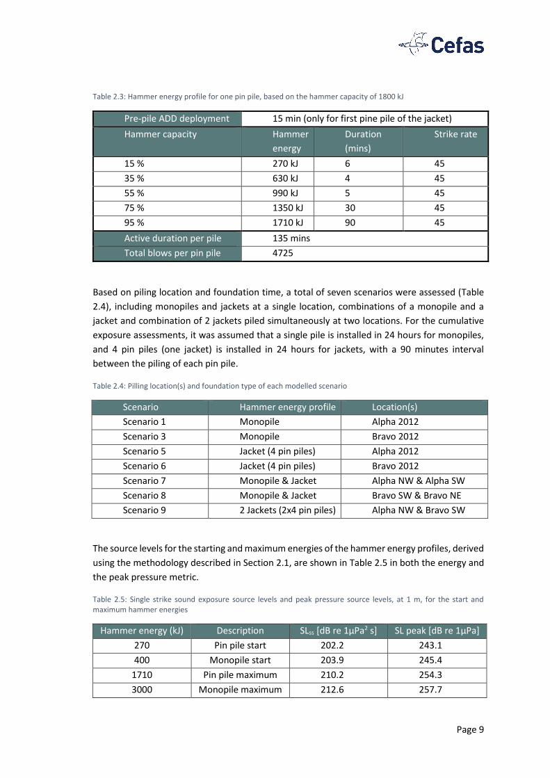
Table 2.3: Hammer energy profile for one pin pile, based on the hammer capacity of 1800 kJ . 9

Table 2.4: Pilling location(s) and foundation type of each modelled scenario ............................ 9

Table 2.5: Single strike sound exposure source levels and peak pressure source levels, at 1 m,

for the start and maximum hammer energies ............................................................................. 9

Table 2.6: Metrics and associated effects for each of the three model types ........................... 10

Table 2.7 NOAA criteria sound exposure thresholds for marine mammals (National Marine

Fisheries Service, 2016) .............................................................................................................. 11

Table 2.8 Southall criteria sound exposure thresholds for marine mammals (Southall et al. 2007)

.................................................................................................................................................... 11

Table 2.9 Sound exposure thresholds for fish (Popper et al., 2014) .......................................... 11

Table 2.10 Fleeing speeds assumed for each marine mammal species/taxon .......................... 12

Page iii

Table 3.1: Scenario list for SELss .................................................................................................. 13

Table 3.2: Effect ranges for instantaneous PTS for marine mammals at the initial hammer energy

(400 kJ for monopiles and 270 kJ for pin piles) .......................................................................... 17

Table 3.3: Effect ranges for instantaneous PTS for marine mammals at the maximum hammer

energy (3000 kJ for monopiles and 1710 kJ for pin piles) .......................................................... 18

Table 3.4: Effect areas for cumulative PTS according to the Southall and NOAA SELcum criteria for

each marine mammal functional hearing group and scenario................................................... 18

Table 3.5: Effect areas for mortality, recoverable injury, and TTS according to the Popper SELcum

criterion for herring .................................................................................................................... 19

Figures

Figure 3-1: Single-strike SEL for a hammer energy of 3000 kJ (maximum monopile hammer

energy) at location Alpha 2012 (Scenario 1) .............................................................................. 14

Figure 3-2: Single-strike SEL for a hammer energy of 3000 kJ (maximum monopile hammer

energy) at location Bravo 2012 (Scenario 3) .............................................................................. 14

Figure 3-3: Single-strike SEL for a hammer energy of 1710 kJ (maximum pin pile hammer energy)

at location Alpha 2012 (Scenario 5) ............................................................................................ 15

Figure 3-4: Single-strike SEL for a hammer energy of 1710 kJ (maximum pin pile hammer energy)

at location Bravo 2012 (Scenario 6) ............................................................................................ 15

Figure 3-5: Combined single-strike SEL for a hammer energy of 3000 kJ (maximum monopile

hammer energy) at location Alpha NW and a hammer energy of 1710 kJ (maximum pin pile

hammer energy) at location Alpha SW (Scenario 7) .................................................................. 16

Figure 3-6: Combined single-strike SEL for a hammer energy of 3000 kJ (maximum monopile

hammer energy) at location Bravo SW and a hammer energy of 1710 kJ (maximum pin pile

hammer energy) at location Bravo NE (Scenario 8) ................................................................... 16

Figure 3-7: Combined Single-strike SEL for a hammer energy of 1710 kJ (maximum pin pile

hammer energy) at locations Alpha NW and Bravo SW (Scenario 9) ......................................... 17

Table 3.2: Effect ranges for instantaneous PTS for marine mammals at the initial hammer energy

(400 kJ for monopiles and 270 kJ for pin piles) .......................................................................... 17

Table 3.3: Effect ranges for instantaneous PTS for marine mammals at the maximum hammer

energy (3000 kJ for monopiles and 1710 kJ for pin piles) .......................................................... 18

Page iv

Table 3.4: Effect areas for cumulative PTS according to the Southall and NOAA SELcum criteria for

each marine mammal functional hearing group and scenario................................................... 18

Table 3.5: Effect areas for mortality, recoverable injury, and TTS according to the Popper SELcum

criterion for herring .................................................................................................................... 19

Figure 3-8: Cumulative exposure effect zones for herring exposed to piling of a single monopile

foundation at location Alpha 2012 (Scenario 1) ......................................................................... 19

Figure 3-9: Cumulative exposure effect zones for herring exposed to piling of a single monopile

foundation at location Bravo 2012 (Scenario 3) ......................................................................... 20

Figure 3-10: Cumulative exposure effect zones for herring exposed to piling of a single jacket

foundation (4 pin piles) at location Alpha 2012 (Scenario 5) ..................................................... 20

Figure 3-11: Cumulative exposure effect zones for herring exposed to piling of a single jacket

foundation (4 pin piles) at location Bravo 2012 (Scenario 6) ..................................................... 21

Figure 3-12: Cumulative exposure effect zones for herring exposed to concomitant piling of a

monopile foundation at location Alpha NW and a jacket foundation (4 pin piles) at location

Alpha SW (Scenario 7) ................................................................................................................ 21

Figure 3-13: Cumulative exposure effect zones for herring exposed to concomitant piling of a

monopile foundation at location Bravo SW and a jacket foundation (4 pin piles) at location Bravo

NE (Scenario 8)............................................................................................................................ 22

Figure 3-14: Cumulative exposure effect zones for herring exposed to concomitant piling of two

jacket foundations (4 pin piles per jacket) at locations Alpha NW and Bravo SW, respectively

(Scenario 9) ................................................................................................................................. 22

Page 5

1 Introduction

This report presents the results of underwater noise modelling carried out by Cefas in support

of the environmental impact assessment for the optimised Seagreen Offshore Wind Farm. The

consented Seagreen Project includes jacket foundation structures with pin pile foundations, the

optimised Seagreen Project proposes monopiles or pin piled jackets. Predictions were made of

the sound exposure levels (SELs) and peak sound pressure levels (peak SPLs) arising from

percussive pile driving for maximal hammer energies of 3,000 kJ (monopiles) and 1,710 kJ (pin

piles, representing 95% of the full hammer capacity of 1800 kJ1) at several locations around the

perimeter of the Development site, including concurrent piling at two locations. Based on these

predictions, effect zones were computed for the risk of permanent threshold shift (PTS) on

harbour porpoise (Phocoena phocoena), bottlenose dolphin (Tursiops truncatus), white-beaked

dolphin (Lagenorhynchus albirostris), minke whale (Balaenoptera acutorostrata), grey seal

(Halichoerus grypus), and harbour seal (Phoca vitulina), using the Southall (Southall et al. 2007)

and NOAA (National marine Fisheries Service, 2016) noise exposure criteria for marine

mammals. Furthermore, the risk of temporary threshold shift (TTS), recoverable injury, and

mortality was predicted for herring (Clupea harengus), based on the Popper et al. (2014)

criteria.

1 This reflects the ramp up for jacket pin piles assumed for the 2012 Offshore ES.

Page 6

2 Methodology

2.1 Source model

The source level estimate for pile driving was calculated using an energy conversion model (De

Jong and Ainslie, 2008), whereby a proportion of the expected hammer energy is converted to

acoustic energy:

𝑺𝑳𝑬 = 𝟏𝟐𝟎 + 𝟏𝟎𝒍𝒐𝒈𝟏𝟎 (𝜷𝑬𝒄𝟎𝝆

𝟒𝝅)

(1)

where 𝐸 is the hammer energy in joules, 𝑆𝐿𝐸 is the source level energy for a single strike at

hammer energy 𝐸, 𝜷 is the acoustic energy conversion efficiency, 𝑐0 is the speed of sound in

seawater in m s-1, and 𝜌 is the density of seawater in kg m-3.

This yields an estimate of the source level in units of sound exposure level (dB re 1 µPa2 s). This

energy is then distributed across the frequency spectrum based on previous measurements of

impact piling (Ainslie et al., 2012).

Hammer energy profiles for the piling scenarios (see Section 0) formed the basis of the source

level estimates. Equation 1 was used to compute the source level energies, using an acoustic

energy conversion efficiency of 0.5%, which assumes that 0.5% of the hammer energy is

converted into acoustic energy. This energy conversion factor is in keeping with current

understanding of how much hammer energy is converted to noise (Dahl and Reinhall, 2013;

Zampolli et al., 2013; Dahl et al., 2015). Equation (1) gives the source level energy for a single

strike (single-strike SEL). The maximal single-pulse SEL, SELss, as well as the cumulative SEL (the

total SEL generated during a specified period), SELcum, were computed.

The peak SPL was calculated using the empirical linear equations linking peak sound pressure

levels and sound exposure levels for pile driving sources found by Lippert et al. (2015).

2.2 Propagation model

The propagation of piling noise was modelled using the Cefas noise model (Farcas et al., 2016),

which is based on a parabolic equation solution to the wave equation (RAM; Collins, 1993).

Unlike many propagation models, this model takes into account the bathymetry, sediment

properties, water column properties, and tidal cycle, leading to more detailed and reliable

predictions of sound level. It is also widely used in peer-reviewed scientific studies which have

benchmarked it against empirical data.

The Cefas model is a quasi-3D model consisting of 360 2D transects extending away from the

source at intervals of one degree. Sound propagation is modelled at each discrete frequency in

the source spectrum (10 frequencies per 1/3 octave band). These transects were then

resampled and integrated over frequency (using the appropriate auditory weightings where

needed). Finally, the resulting levels were averaged over depth to produce noise maps.

Page 7

2.3 Input data

Aside from source levels of piling, the main model inputs were bathymetry, water temperature

and salinity (used to compute sound speed), and the acoustic properties of the seabed

sediments.

Bathymetric data in UTM30N projection was provided to Cefas, covering the area inside the

Project Alpha and Project Bravo boundaries. This was supplemented by a more extensive

dataset, with a 7.5” resolution and in WGS84 projection, which was downloaded from

EMODNET database (http://www.emodnet-bathymetry.eu/data-products) and then converted

to UTM30N projection. The bathymetric datasets were interpolated and used to define the

model numerical grid with a resolution of 100 m, and a coverage of 500000-750000, 6100000-

6500000 (eastings, northings UTM30N), or approximately 250 km by 400 km, which was more

than adequate for the frequency ranges and the spatial scales used in the simulations.

The water temperature and salinity data, which are used by the model for calculating the water

column sound speed profiles, were taken from a validated, multiyear hindcast model produced

by Cefas, known as GETM-ERSEM-BFM. The model provides extensive daily coverage at 0.1

degree spatial resolution, and includes 25 depth layers. Typical November water properties

were used for the acoustic propagation predictions, representing a midpoint between winter

and summer sound propagating conditions. It was chosen to model water properties based on

a typical November as this represents a mixture of most probable and worst-case scenarios

which would form a conservative but probable scenario.

The noise model also includes the acoustic properties of the seabed sediments, namely speed

of sound, density, and acoustic attenuation, which are used to construct a geoacoustic model

of the seafloor. These properties were derived from the seabed core data by correlating the

core sediment information with published acoustic properties of various sediment types

(Hamilton, 1980).

2.4 Piling Locations

The piling locations that were modelled in the assessment and their coordinates are given in

Table 2.1. These locations, and piling parameters summarised below, were provided to Cefas

by NIRAS Consulting, the Project Lead EIA consultants, following consultation with Marine

Scotland and Scottish Natural Heritage.

Table 2.1 Pile driving locations used for noise modelling with coordinates in decimal degrees

Location Latitude Longitude

Alpha 2012 56.5929 -1.9301

Bravo 2012 56.5897 -1.7328

Alpha NW 56.677553 -1.937101

Alpha SW 56.513386 -1.939632

Bravo SW 56.515385 -1.892356

Page 8

Location Latitude Longitude

Bravo NE 56.665388 -1.577116

2.5 Piling Scenarios

Hammer energy profiles were estimated for driving monopiles of 10 m diameter for the worst-

case ground conditions at the site, with a maximum hammer energy of 3000 kJ (Table 2.2), and

for driving pin piles of 2 m diameter (Table 2.3), with a maximum hammer energy of 1710 kJ

(representing 95% of the full hammer capacity of 1800 kJ).

Table 2.2: Monopile hammer energy profile

Pre-pile ADD deployment duration 15 min

A. Soft start initiation

Soft start A starting energy 400 kJ

Soft start A energy ramp up none

Soft start A duration 1 min

Soft start A strike rate 7 blows/min

Soft start A end energy 400 kJ

B. Soft start Soft start B starting energy 400 kJ

Soft start B energy ramp up even

Soft start B duration 19 min

Soft start B strike rate 31 blows/min

Soft start B end energy 600 kJ

C. Progression to Full Power

Piling C starting energy 600 kJ

Piling C energy ramp up even

Piling C duration 120 min

Piling C strike rate 35 blows/min

Piling C end energy 3000 kJ

D. Full Power Piling

Piling D starting energy 3000 kJ

Piling D energy ramp up none

Piling D duration 100 min

Piling D strike rate 35 blows/min

Piling D end energy 3000 kJ

Total active piling duration (min) 240 min

Total blows 8296

Page 9

Table 2.3: Hammer energy profile for one pin pile, based on the hammer capacity of 1800 kJ

Pre-pile ADD deployment 15 min (only for first pine pile of the jacket)

Hammer capacity Hammer

energy

Duration

(mins)

Strike rate

15 % 270 kJ 6 45

35 % 630 kJ 4 45

55 % 990 kJ 5 45

75 % 1350 kJ 30 45

95 % 1710 kJ 90 45

Active duration per pile 135 mins

Total blows per pin pile 4725

Based on piling location and foundation time, a total of seven scenarios were assessed (Table

2.4), including monopiles and jackets at a single location, combinations of a monopile and a

jacket and combination of 2 jackets piled simultaneously at two locations. For the cumulative

exposure assessments, it was assumed that a single pile is installed in 24 hours for monopiles,

and 4 pin piles (one jacket) is installed in 24 hours for jackets, with a 90 minutes interval

between the piling of each pin pile.

Table 2.4: Pilling location(s) and foundation type of each modelled scenario

Scenario Hammer energy profile Location(s)

Scenario 1 Monopile Alpha 2012

Scenario 3 Monopile Bravo 2012

Scenario 5 Jacket (4 pin piles) Alpha 2012

Scenario 6 Jacket (4 pin piles) Bravo 2012

Scenario 7 Monopile & Jacket Alpha NW & Alpha SW

Scenario 8 Monopile & Jacket Bravo SW & Bravo NE

Scenario 9 2 Jackets (2x4 pin piles) Alpha NW & Bravo SW

The source levels for the starting and maximum energies of the hammer energy profiles, derived

using the methodology described in Section 2.1, are shown in Table 2.5 in both the energy and

the peak pressure metric.

Table 2.5: Single strike sound exposure source levels and peak pressure source levels, at 1 m, for the start and maximum hammer energies

Hammer energy (kJ) Description SLss [dB re 1µPa2 s] SL peak [dB re 1µPa]

270 Pin pile start 202.2 243.1

400 Monopile start 203.9 245.4

1710 Pin pile maximum 210.2 254.3

3000 Monopile maximum 212.6 257.7

Page 10

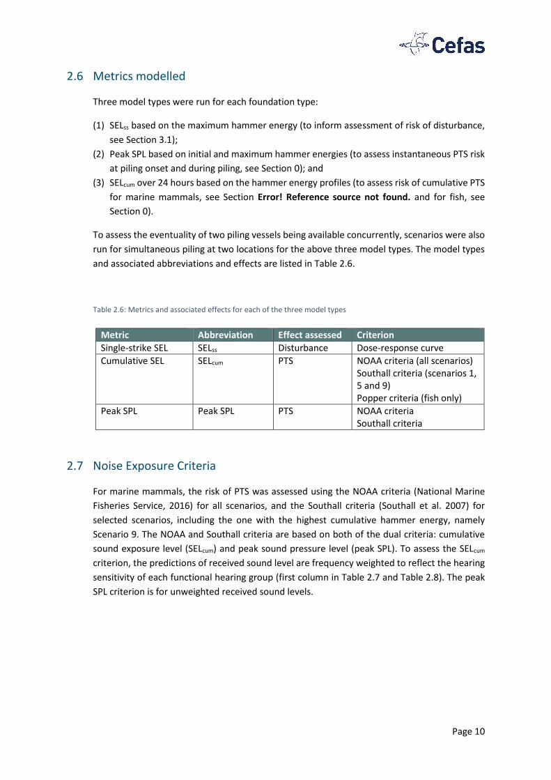
2.6 Metrics modelled

Three model types were run for each foundation type:

(1) SELss based on the maximum hammer energy (to inform assessment of risk of disturbance,

see Section 3.1);

(2) Peak SPL based on initial and maximum hammer energies (to assess instantaneous PTS risk

at piling onset and during piling, see Section 0); and

(3) SELcum over 24 hours based on the hammer energy profiles (to assess risk of cumulative PTS

for marine mammals, see Section Error! Reference source not found. and for fish, see

Section 0).

To assess the eventuality of two piling vessels being available concurrently, scenarios were also

run for simultaneous piling at two locations for the above three model types. The model types

and associated abbreviations and effects are listed in Table 2.6.

Table 2.6: Metrics and associated effects for each of the three model types

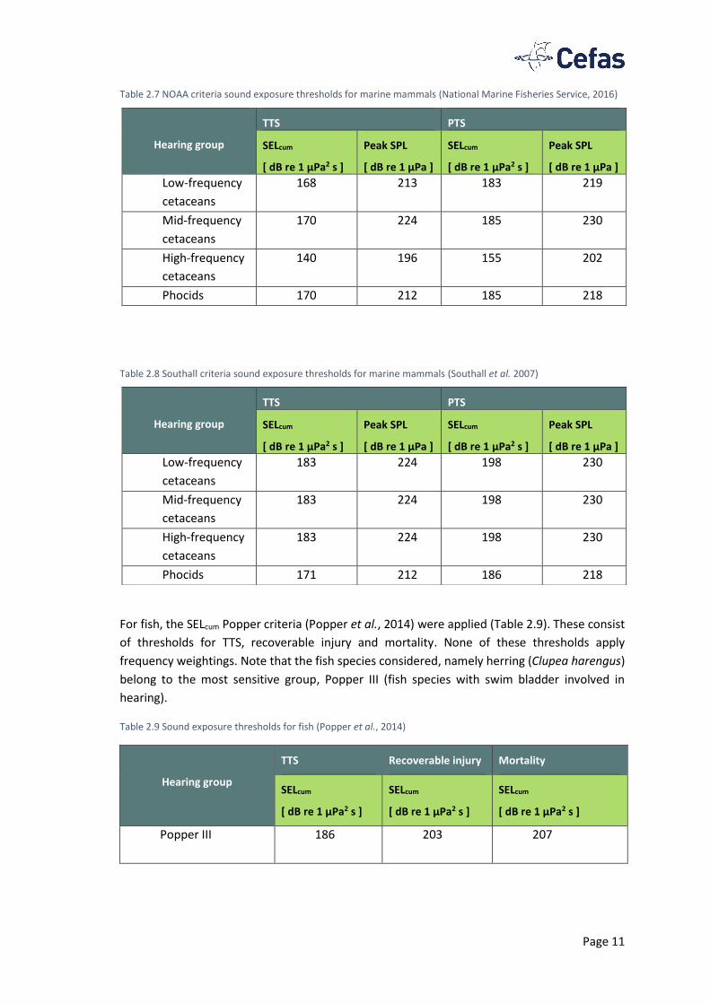
2.7 Noise Exposure Criteria

For marine mammals, the risk of PTS was assessed using the NOAA criteria (National Marine

Fisheries Service, 2016) for all scenarios, and the Southall criteria (Southall et al. 2007) for

selected scenarios, including the one with the highest cumulative hammer energy, namely

Scenario 9. The NOAA and Southall criteria are based on both of the dual criteria: cumulative

sound exposure level (SELcum) and peak sound pressure level (peak SPL). To assess the SELcum

criterion, the predictions of received sound level are frequency weighted to reflect the hearing

sensitivity of each functional hearing group (first column in Table 2.7 and Table 2.8). The peak

SPL criterion is for unweighted received sound levels.

Metric Abbreviation Effect assessed Criterion

Single-strike SEL SELss Disturbance Dose-response curve

Cumulative SEL SELcum PTS NOAA criteria (all scenarios) Southall criteria (scenarios 1, 5 and 9) Popper criteria (fish only)

Peak SPL Peak SPL PTS NOAA criteria Southall criteria

Page 11

Table 2.7 NOAA criteria sound exposure thresholds for marine mammals (National Marine Fisheries Service, 2016)

Table 2.8 Southall criteria sound exposure thresholds for marine mammals (Southall et al. 2007)

For fish, the SELcum Popper criteria (Popper et al., 2014) were applied (Table 2.9). These consist

of thresholds for TTS, recoverable injury and mortality. None of these thresholds apply

frequency weightings. Note that the fish species considered, namely herring (Clupea harengus)

belong to the most sensitive group, Popper III (fish species with swim bladder involved in

hearing).

Table 2.9 Sound exposure thresholds for fish (Popper et al., 2014)

Hearing group

TTS Recoverable injury Mortality

SELcum

[ dB re 1 μPa2 s ]

SELcum

[ dB re 1 μPa2 s ]

SELcum

[ dB re 1 μPa2 s ]

Popper III 186

203 207

Hearing group

TTS PTS

SELcum

[ dB re 1 μPa2 s ]

Peak SPL

[ dB re 1 μPa ]

SELcum

[ dB re 1 μPa2 s ]

Peak SPL

[ dB re 1 μPa ]

Low-frequency

cetaceans

168 213 183 219

Mid-frequency

cetaceans

170 224 185 230

High-frequency

cetaceans

140 196 155 202

Phocids 170 212 185 218

Hearing group

TTS PTS

SELcum

[ dB re 1 μPa2 s ]

Peak SPL

[ dB re 1 μPa ]

SELcum

[ dB re 1 μPa2 s ]

Peak SPL

[ dB re 1 μPa ]

Low-frequency

cetaceans

183 224 198 230

Mid-frequency

cetaceans

183 224 198 230

High-frequency

cetaceans

183 224 198 230

Phocids 171 212 186 218

Page 12

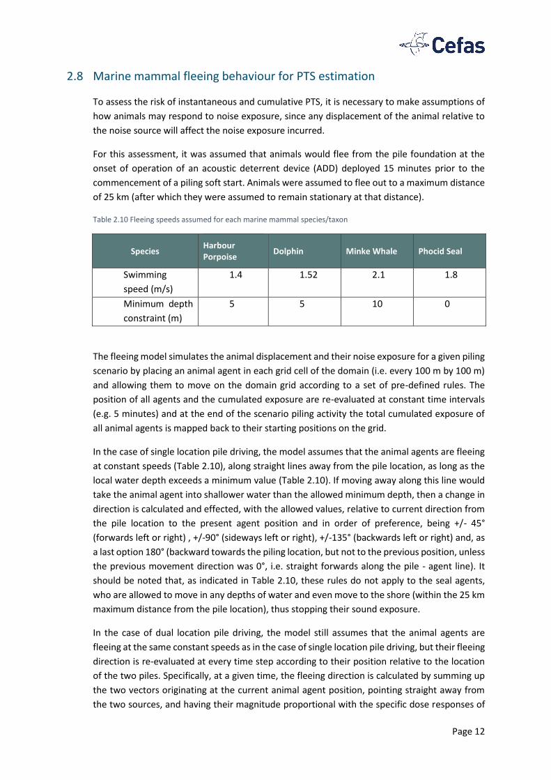
2.8 Marine mammal fleeing behaviour for PTS estimation

To assess the risk of instantaneous and cumulative PTS, it is necessary to make assumptions of

how animals may respond to noise exposure, since any displacement of the animal relative to

the noise source will affect the noise exposure incurred.

For this assessment, it was assumed that animals would flee from the pile foundation at the

onset of operation of an acoustic deterrent device (ADD) deployed 15 minutes prior to the

commencement of a piling soft start. Animals were assumed to flee out to a maximum distance

of 25 km (after which they were assumed to remain stationary at that distance).

Table 2.10 Fleeing speeds assumed for each marine mammal species/taxon

Species Harbour Porpoise

Dolphin Minke Whale Phocid Seal

Swimming

speed (m/s)

1.4 1.52 2.1 1.8

Minimum depth

constraint (m)

5 5 10 0

The fleeing model simulates the animal displacement and their noise exposure for a given piling

scenario by placing an animal agent in each grid cell of the domain (i.e. every 100 m by 100 m)

and allowing them to move on the domain grid according to a set of pre-defined rules. The

position of all agents and the cumulated exposure are re-evaluated at constant time intervals

(e.g. 5 minutes) and at the end of the scenario piling activity the total cumulated exposure of

all animal agents is mapped back to their starting positions on the grid.

In the case of single location pile driving, the model assumes that the animal agents are fleeing

at constant speeds (Table 2.10), along straight lines away from the pile location, as long as the

local water depth exceeds a minimum value (Table 2.10). If moving away along this line would

take the animal agent into shallower water than the allowed minimum depth, then a change in

direction is calculated and effected, with the allowed values, relative to current direction from

the pile location to the present agent position and in order of preference, being +/- 45°

(forwards left or right) , +/-90° (sideways left or right), +/-135° (backwards left or right) and, as

a last option 180° (backward towards the piling location, but not to the previous position, unless

the previous movement direction was 0°, i.e. straight forwards along the pile - agent line). It

should be noted that, as indicated in Table 2.10, these rules do not apply to the seal agents,

who are allowed to move in any depths of water and even move to the shore (within the 25 km

maximum distance from the pile location), thus stopping their sound exposure.

In the case of dual location pile driving, the model still assumes that the animal agents are

fleeing at the same constant speeds as in the case of single location pile driving, but their fleeing

direction is re-evaluated at every time step according to their position relative to the location

of the two piles. Specifically, at a given time, the fleeing direction is calculated by summing up

the two vectors originating at the current animal agent position, pointing straight away from

the two sources, and having their magnitude proportional with the specific dose responses of

Page 13

the animal for the current single strike SEL from the two sources, respectively. The same

minimum depth constrains and shallow water avoidance rules as in the single location pile

driving described above apply also in the case of dual location pile driving.

3 Results

3.1 Single-Strike Sound Exposure Levels for Behavioural Response Assessment

The scenario assessed for SELss are listed in Table 3.1 and the results are shown in Figure 3-1 to

Figure 3-7. Scenario numbering is non-sequential because Scenarios 2 and 4 (2,300 kJ monopile

installation at Alpha and Bravo respectively) were not pursued following review of the results

of higher energy piling (scenarios 1 and 3) at the same locations.

Table 3.1: Scenario list for SELss

Scenario Description Figure number

Scenario 1 3000 kJ at Alpha 2012 Figure 3-1

Scenario 3 3000 kJ Bravo 2012 Figure 3-2

Scenario 5 1710 kJ at Alpha 2012 Figure 3-3

Scenario 6 1710 kJ at Bravo 2012 Figure 3-4

Scenario 7 3000 kJ at Alpha NW &

1710 kJ at Alpha SW

Figure 3-5

Scenario 8 3000 kJ at Bravo SW &

1710 kJ at Bravo NE

Figure 3-6

Scenario 9 1710 kJ at Alpha NW &

1710 kJ at Bravo SW

Figure 3-7

Page 14

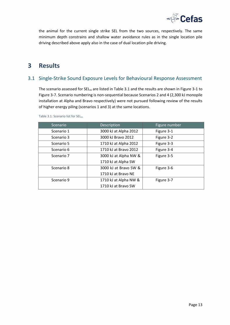
Figure 3-1: Single-strike SEL for a hammer energy of 3000 kJ (maximum monopile hammer energy) at location Alpha 2012 (Scenario 1)

Figure 3-2: Single-strike SEL for a hammer energy of 3000 kJ (maximum monopile hammer energy) at location Bravo 2012 (Scenario 3)

Page 15

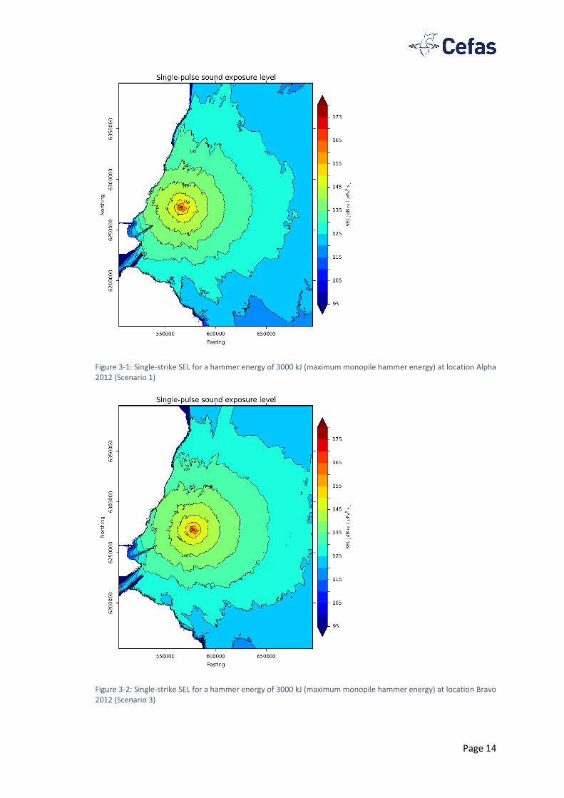
Figure 3-3: Single-strike SEL for a hammer energy of 1710 kJ (maximum pin pile hammer energy) at location Alpha 2012 (Scenario 5)

Figure 3-4: Single-strike SEL for a hammer energy of 1710 kJ (maximum pin pile hammer energy) at location Bravo 2012 (Scenario 6)

Page 16

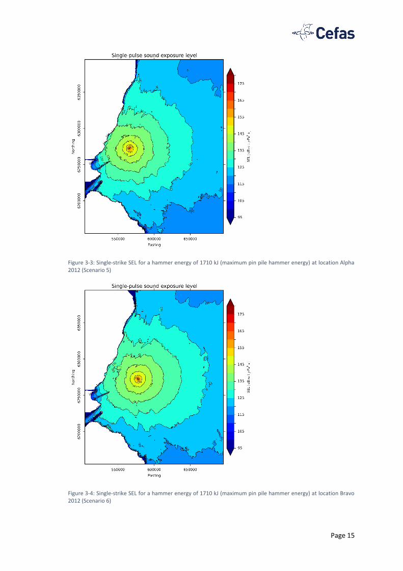
Figure 3-5: Combined single-strike SEL for a hammer energy of 3000 kJ (maximum monopile hammer energy) at location Alpha NW and a hammer energy of 1710 kJ (maximum pin pile hammer energy) at location Alpha SW (Scenario 7)

Figure 3-6: Combined single-strike SEL for a hammer energy of 3000 kJ (maximum monopile hammer energy) at location Bravo SW and a hammer energy of 1710 kJ (maximum pin pile hammer energy) at location Bravo NE (Scenario 8)

Page 17

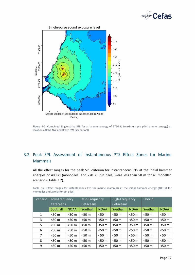
Figure 3-7: Combined Single-strike SEL for a hammer energy of 1710 kJ (maximum pin pile hammer energy) at locations Alpha NW and Bravo SW (Scenario 9)

3.2 Peak SPL Assessment of Instantaneous PTS Effect Zones for Marine

Mammals

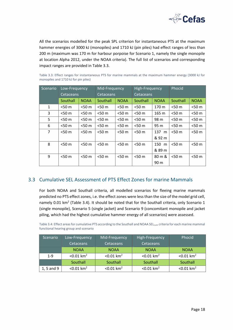
All the effect ranges for the peak SPL criterion for instantaneous PTS at the initial hammer

energies of 400 kJ (monopiles) and 270 kJ (pin piles) were less than 50 m for all modelled

scenarios (Table 3.2).

Table 3.2: Effect ranges for instantaneous PTS for marine mammals at the initial hammer energy (400 kJ for monopiles and 270 kJ for pin piles)

Scenario Low-Frequency

Cetaceans

Mid-Frequency

Cetaceans

High-Frequency

Cetaceans

Phocid

Southall NOAA Southall NOAA Southall NOAA Southall NOAA

1 <50 m <50 m <50 m <50 m <50 m <50 m <50 m <50 m

3 <50 m <50 m <50 m <50 m <50 m <50 m <50 m <50 m

5 <50 m <50 m <50 m <50 m <50 m <50 m <50 m <50 m

6 <50 m <50 m <50 m <50 m <50 m <50 m <50 m <50 m

7 <50 m <50 m <50 m <50 m <50 m <50 m <50 m <50 m

8 <50 m <50 m <50 m <50 m <50 m <50 m <50 m <50 m

9 <50 m <50 m <50 m <50 m <50 m <50 m <50 m <50 m

Page 18

All the scenarios modelled for the peak SPL criterion for instantaneous PTS at the maximum

hammer energies of 3000 kJ (monopiles) and 1710 kJ (pin piles) had effect ranges of less than

200 m (maximum was 170 m for harbour porpoise for Scenario 1, namely the single monopile

at location Alpha 2012, under the NOAA criteria). The full list of scenarios and corresponding

impact ranges are provided in Table 3.3.

Table 3.3: Effect ranges for instantaneous PTS for marine mammals at the maximum hammer energy (3000 kJ for monopiles and 1710 kJ for pin piles)

Scenario Low-Frequency

Cetaceans

Mid-Frequency

Cetaceans

High-Frequency

Cetaceans

Phocid

Southall NOAA Southall NOAA Southall NOAA Southall NOAA

1 <50 m <50 m <50 m <50 m <50 m 170 m <50 m <50 m

3 <50 m <50 m <50 m <50 m <50 m 165 m <50 m <50 m

5 <50 m <50 m <50 m <50 m <50 m 98 m <50 m <50 m

6 <50 m <50 m <50 m <50 m <50 m 95 m <50 m <50 m

7 <50 m <50 m <50 m <50 m <50 m 137 m

& 92 m

<50 m <50 m

8 <50 m <50 m <50 m <50 m <50 m 150 m

& 89 m

<50 m <50 m

9 <50 m <50 m <50 m <50 m <50 m 80 m &

90 m

<50 m <50 m

3.3 Cumulative SEL Assessment of PTS Effect Zones for marine Mammals

For both NOAA and Southall criteria, all modelled scenarios for fleeing marine mammals

predicted no PTS effect zones, i.e. the effect zones were less than the size of the model grid cell,

namely 0.01 km2 (Table 3.4). It should be noted that for the Southall criteria, only Scenario 1

(single monopile), Scenario 5 (single jacket) and Scenario 9 (concomitant monopile and jacket

piling, which had the highest cumulative hammer energy of all scenarios) were assessed.

Table 3.4: Effect areas for cumulative PTS according to the Southall and NOAA SELcum criteria for each marine mammal functional hearing group and scenario

Scenario Low-Frequency

Cetaceans

Mid-Frequency

Cetaceans

High-Frequency

Cetaceans

Phocid

NOAA NOAA NOAA NOAA

1-9 <0.01 km2 <0.01 km2 <0.01 km2 <0.01 km2

Southall Southall Southall Southall

1, 5 and 9 <0.01 km2 <0.01 km2 <0.01 km2 <0.01 km2

Page 19

3.4 Cumulative SEL Assessment of TTS, Recoverable Injury, and Mortality Effect

Zones for Fish

Mortality, recoverable injury, and TTS effect zones were predicted for all seven scenarios

assessed for herring (i.e. Group III fish species) (Table 3.5). Maps of these effect zones are shown

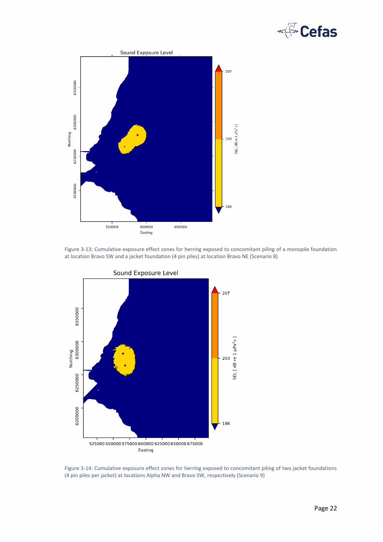
in Figure 3-8 to Figure 3-14. The largest effect zones (2.83 km2 mortality, 8.83 km2 for

recoverable injury and 1275.45 km2 for TTS) were predicted for concomitant piling of two jacket

foundations (Scenario 9, Figure 3-14), which had the highest cumulative hammer energy from

all the scenarios assessed.

Table 3.5: Effect areas for mortality, recoverable injury, and TTS according to the Popper SELcum criterion for herring

Scenario TTS area (km2);

range (m)

Recoverable injury

area (km2); range (m)

Mortality area

(km2); range (m)

Figure number

Scenario 1 268.64; 10,638 1.98; 804 0.04; 141 Figure 3-8

Scenario 3 297.01; 10,509 1.95; 822 0.01; 50 Figure 3-9

Scenario 5 593.39; 15,863 5.21; 1,354 1.64; 726 Figure 3-10

Scenario 6 665.42; 16,932 4.96; 1,312 1.58; 726 Figure 3-11

Scenario 7 970.83 6.55 1.5 Figure 3-12

Scenario 8 1057.64 6.4 1.38 Figure 3-13

Scenario 9 1275.45 8.83 2.83 Figure 3-14

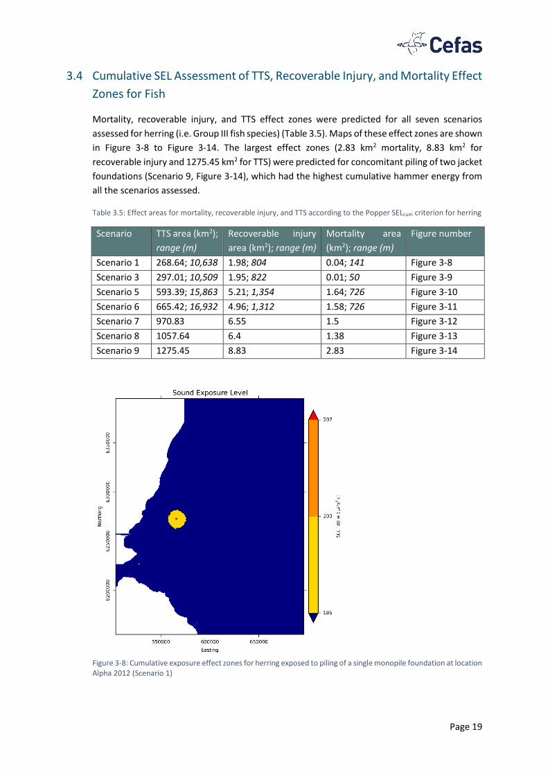
Figure 3-8: Cumulative exposure effect zones for herring exposed to piling of a single monopile foundation at location Alpha 2012 (Scenario 1)

Page 20

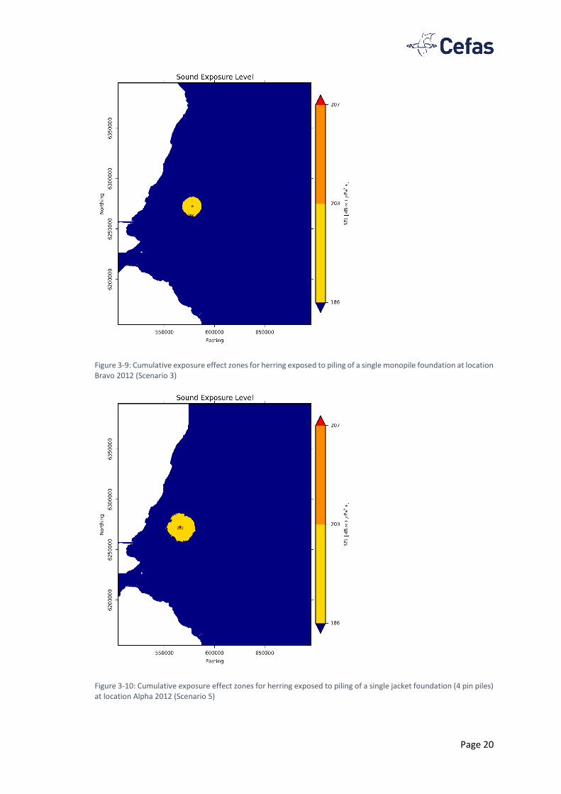
Figure 3-9: Cumulative exposure effect zones for herring exposed to piling of a single monopile foundation at location Bravo 2012 (Scenario 3)

Figure 3-10: Cumulative exposure effect zones for herring exposed to piling of a single jacket foundation (4 pin piles) at location Alpha 2012 (Scenario 5)

Page 21

Figure 3-11: Cumulative exposure effect zones for herring exposed to piling of a single jacket foundation (4 pin piles) at location Bravo 2012 (Scenario 6)

Figure 3-12: Cumulative exposure effect zones for herring exposed to concomitant piling of a monopile foundation at location Alpha NW and a jacket foundation (4 pin piles) at location Alpha SW (Scenario 7)

Page 22

Figure 3-13: Cumulative exposure effect zones for herring exposed to concomitant piling of a monopile foundation at location Bravo SW and a jacket foundation (4 pin piles) at location Bravo NE (Scenario 8)

Figure 3-14: Cumulative exposure effect zones for herring exposed to concomitant piling of two jacket foundations (4 pin piles per jacket) at locations Alpha NW and Bravo SW, respectively (Scenario 9)

Page 23

4 References

Ainslie, M.A., de Jong, C.A.F., Robinson, S.P. & Lepper, P.A. (2012). What is the source level of pile-

driving noise in water? In: Eff. Noise Aquat. Life (eds. Popper, A.N. & Hawkins, A.D.). Springer, NY, pp.

445–448.

Collins, M.D. (1993). A split-step Padé solution for the parabolic equation method. J. Acoust. Soc. Am.,

93, 1736–1742.

Dahl, P.H., de Jong, C.A.F. & Popper, A.N. (2015). The Underwater Sound Field from Impact Pile Driving

and Its Potential Effects on Marine Life. Acoust. Today, 11.

Dahl, P.H. & Reinhall, P.G. (2013). Beam forming of the underwater sound field from impact pile

driving. J. Acoust. Soc. Am., 134, EL1-6.

Etter, P.C. (2013). Underwater acoustic modeling and simulation. CRC Press, FL.

Farcas, A., Thompson, P.M. & Merchant, N.D. (2016). Underwater noise modelling for environmental

impact assessment. Environ. Impact Assess. Rev., 57, 114–122.

Jensen, F.B., Kuperman, W.A., Porter, M.B. & Schmidt, H. (2011). Computational ocean acoustics.

Springer, NY.

De Jong, C.A. f & Ainslie, M.A. (2008). Underwater radiated noise due to the piling for the Q7 Offshore

Wind Park. J. Acoust. Soc. Am., 123, 2987.

Lippert, T., Galindo-Romero, M., Gavrilov, A.N. & von Estorff, O. (2015) Empirical estimation of peak

pressure level from sound exposure level. Part II: Offshore impact pile driving noise. The Journal of the

Acoustical Society of America, 138 (3), EL287-EL292.

National Marine Fisheries Service. (2016). Technical Guidance for Assessing the Effects of

Anthropogenic Sound on Marine Mammal Hearing: Underwater Acoustic Thresholds for Onset of

Permanent and Temporary Threshold Shifts. U.S. Dept. of Commer., NOAA. NOAA Technical

Memorandum NMFS-OPR-55, 178 p.

Popper, A.N., Hawkins, A.D., Fay, R.R., Mann, D.A., Bartol, S., Carlson, T.J., Coombs, S., Ellison, W.T.,

Gentry, R.L., Halvorsen, M.B., Løkkeborg, S., Rogers, P.H., Southall, B.L., Zeddies, D.G. & Tavolga, W.N.

(2014). ASA S3/SC1.4 TR-2014 Sound Exposure Guidelines for Fishes and Sea Turtles: A Technical

Report prepared by ANSI-Accredited Standards committee S3/SC1 and registered with ANSI. American

National Standards Institute.

Southall, B., Bowles, A., Ellison, W., Finneran, J.J., Gentry, R., Greene, C.R.J., Kastak, D., Ketten, D.,

Miller, J., Nachtigall, P., Richardson, W.J., Thomas, J. & Tyack, P. (2007). Marine mammal noise-

exposure criteria: initial scientific recommendations. Aquat. Mamm., 33, 411–521.

Zampolli, M., Nijhof, M.J.J., de Jong, C.A.F., Ainslie, M.A., Jansen, E.H.W. & Quesson, B.A.J. (2013).

Validation of finite element computations for the quantitative prediction of underwater noise from

impact pile driving. J. Acoust. Soc. Am., 133, 72–81.

© Crown copyright 2016 Printed on paper made from a minimum 75% de-inked post-consumer waste

About us

The Centre for Environment, Fisheries and Aquaculture Science is the UK’s leading and most diverse centre for applied marine and freshwater science. We advise UK government and private sector customers on the environmental impact of their policies, programmes and activities through our scientific evidence and impartial expert advice. Our environmental monitoring and assessment programmes are fundamental to the sustainable development of marine and freshwater industries. Through the application of our science and technology, we play a major role in growing the marine and freshwater economy, creating jobs, and safeguarding public health and the health of our seas and aquatic resources Head office Centre for Environment, Fisheries & Aquaculture Science Pakefield Road Lowestoft Suffolk NR33 0HT Tel: +44 (0) 1502 56 2244 Fax: +44 (0) 1502 51 3865 Weymouth office Barrack Road The Nothe Weymouth DT4 8UB Tel: +44 (0) 1305 206600 Fax: +44 (0) 1305 206601

Customer focus

We offer a range of multidisciplinary bespoke scientific programmes covering a range of sectors, both public and private. Our broad capability covers shelf sea dynamics, climate effects on the aquatic environment, ecosystems and food security. We are growing our business in overseas markets, with a particular emphasis on Kuwait and the Middle East. Our customer base and partnerships are broad, spanning Government, public and private sectors, academia, non-governmental organisations (NGOs), at home and internationally. We work with:

• a wide range of UK Government departments and agencies, including Department for the Environment Food and Rural Affairs (Defra) and Department for Energy and Climate and Change (DECC), Natural Resources Wales, Scotland, Northern Ireland and governments overseas.

• industries across a range of sectors including offshore renewable energy, oil and gas emergency response, marine surveying, fishing and aquaculture.

• other scientists from research councils, universities and EU research programmes.

• NGOs interested in marine and freshwater.

• local communities and voluntary groups, active in protecting the coastal, marine and freshwater environments.

www.cefas.co.uk