Unit 23: ERROR PROPAGATION, DIRECT CURRENT CIRCUITS

Name ______________________ Date(YY/MM/DD) ______/_________/________ St.No. __ __ __ __ __-__ __ __ __ Section_________Group #________

Unit 23: ERROR PROPAGATION, DIRECT CURRENT CIRCUITS1

Estimated classroom time: Two 100 minute sessions

I have a strong resistance to understanding the relationship between voltage and current.

Anonymous Introductory Physics Student

OBJECTIVES

1. To learn to the principles of error propagation when doing calculations.

2. To understand and apply Ohm’s law to a resistor and understand the I vs V characteristics of a non-Ohmic device.

3. To find a mathematical description of the flow of electric current through different elements in direct current circuits (Kirchhoff's laws).

4. To gain experience with basic electronic equipment and the process of constructing useful circuits while reviewing the application of Kirchhoff's laws.

© 1990-93 Dept. of Physics and Astronomy, Dickinson College Supported by FIPSE (U.S. Dept. of Ed.) and NSF. Modified at SFU by N. Alberding & S. Johnson, 2014.

1 Portions of this unit are based on research by Lillian C. McDermott & Peter S. Shaffer published in AJP 60, 994-1012 (1992).

OVERVIEW5 min

We’ll start this unit by understanding how uncertainties of measured quantities affect the uncertainties of values calculated from them. We’ll be using these techniques when comparing experimental results to expected or theoretical values.

Next we’ll continue studying DC circuits. In the last unit you saw that in a series circuit with a battery,1. the current is the same through all elements, 2. changing one part of a series circuit changes the current in all

parts of the circuit,3. the voltage divides between the elements of the series and4. the total of voltages sums to the voltage of the battery.

You also saw that in a parallel circuit with a battery, 1. the current divides among the branches,2. making a change in one branch of a parallel circuit does not

affect the current flowing in the other branch (or branches),3. the total current from the battery equals the sum of the currents

in each branch and 4. the voltage across each branch of a parallel circuit is the same. In this unit, you will first examine the role of the battery as a voltage source and understand how the voltage depends on whether batteries are connected in parallel or series.

We’ll explore the current through electrical devices as a function of the potential difference. Resistors follow Ohm’s law where current is proportional to voltage, but light bulbs do not.

You will measure the effective resistance of resistors when they are wired in series and in parallel. Finally you will formulate the rules for the calculation of the electric current in different parts of complex electric circuits consisting of many resistors and/or batteries wired in series and parallel. These rules are known as Kirchhoff's laws. To test your understanding of Kirchhoff's laws, you will learn to use a breadboard to wire complex electric circuits and verify the voltages and currents predicted by these laws.

Page 23-2 Workshop Physics II Activity Guide SFU


SESSION ONE: PROPAGATION OF ERRORS — USING A DIGITAL MULTIMETER

Propagation of ErrorsAt the beginning of Physics 140 (remember?) we did some activities exploring how random and systematic errors affect measurements we make in physics. This was important because progress in many sciences depends on how accurately a theory can predict the outcome of experiments. We can test the validity of a theory by comparing measured quantities with what the theory predicts. But agreement between theory and measurement is almost never exact so a theory is not considered in disagreement with measurement if the disagreement can be accounted for by the reasonable uncertainties in measurement.

Often a theory predicts a quantity that is not directly measured but depends on a calculation. The measured quantities that contribute to the calculation all have different uncertainties due to random errors. The calculated result has an uncertainty that is determined by the uncertainties of the values used in getting the result. How do we go about determining the uncertainty of the result? There are only a few simple rules.

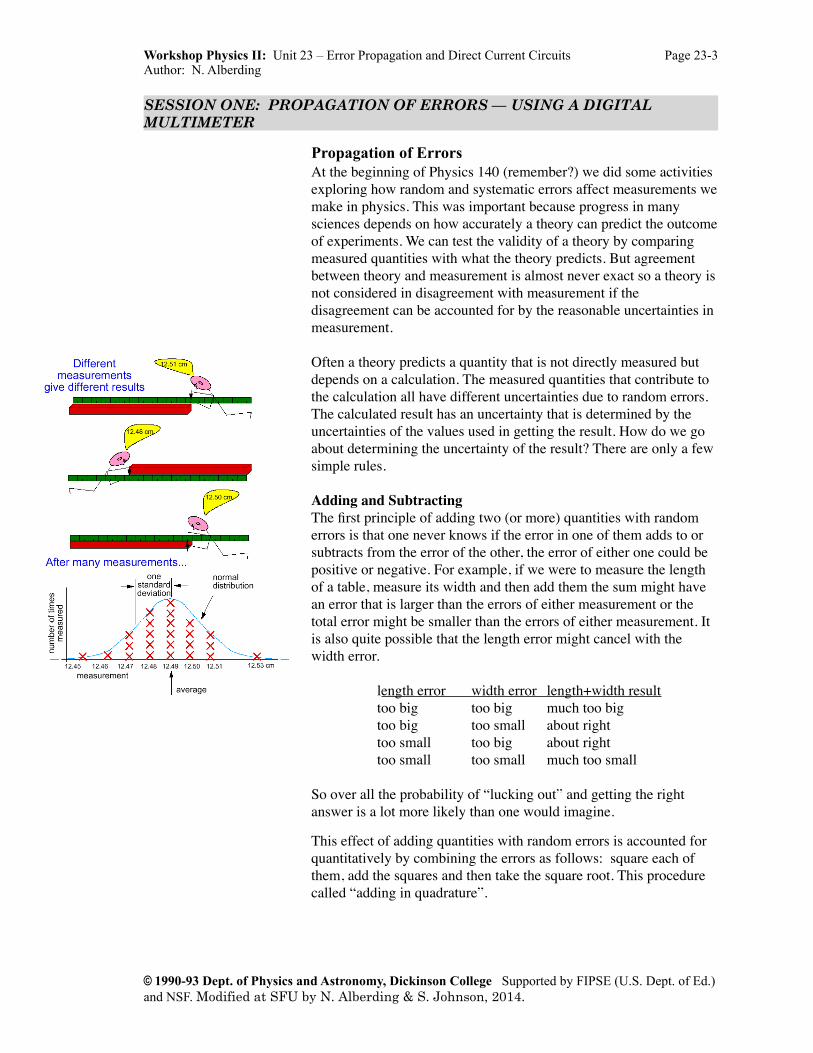
Adding and SubtractingThe first principle of adding two (or more) quantities with random errors is that one never knows if the error in one of them adds to or subtracts from the error of the other, the error of either one could be positive or negative. For example, if we were to measure the length of a table, measure its width and then add them the sum might have an error that is larger than the errors of either measurement or the total error might be smaller than the errors of either measurement. It is also quite possible that the length error might cancel with the width error. length error width error length+width result too big too big much too big too big too small about right too small too big about right too small too small much too small

So over all the probability of “lucking out” and getting the right answer is a lot more likely than one would imagine.

This effect of adding quantities with random errors is accounted for quantitatively by combining the errors as follows: square each of them, add the squares and then take the square root. This procedure called “adding in quadrature”.

Workshop Physics II: Unit 23 – Error Propagation and Direct Current Circuits Page 23-3Author: N. Alberding


For example: length = 1.21 ± 0.04 m width = 0.85 ± 0.03 m

length+width = 2.06 ±

0.042 + 0.032 = 2.06 ± 0.05 m\sqrt0.04^2 + 0.03^2

Naively we might ascribe an error of ±0.07 m to the sum the length and the width. If the two measurement are independent of each other and the errors are random then the result, 0.05 m which we got by adding in quadrature, accounts for the fact that the error of one quantity frequently cancels out with the error of the other.

If we need to subtract quantities, the errors still add in quadrature. After all, we don’t know if the error would be positive or negative so the results is still uncertain by the same amount as if we were adding. Thus

length–width = 0.36 ± 0.05 m

Subtracting two quantities with random errors often results in a small result with a relatively large error.

We can summarize as follows. Let the two measurements and their errors be

x ± Δx and y ± Δy. Then

Δ(x+y) =

(x)2 + (y)2

Multiplying and DividingThe rule for multiplying is similar to that of addition but instead of using the absolute error, Δx, one adds the relative errors, Δx/x, in quadrature. Often one refers to relative error as the percentage error. The relative error of a product of two numbers is got by adding the relative errors of the numbers:

For example

length = 1.91 ± 0.04 m, relative error = 0.04/1.91 ≈ 0.02 or 2%width = 0.45 ± 0.03 m, relative error = 0.03/0.45 ≈ 0.07 or 7%

length x width = 1.91 x 0.45 = 0.859 ± 0.859

(2%)2 + (7%)2 = 0.86 ± 0.06 m2

Notice that when one of the errors is more than double that of the other (7% > 2×2%), the result of adding in quadrature is not much different than just the largest error alone — there’s really no need to calculate in this case.



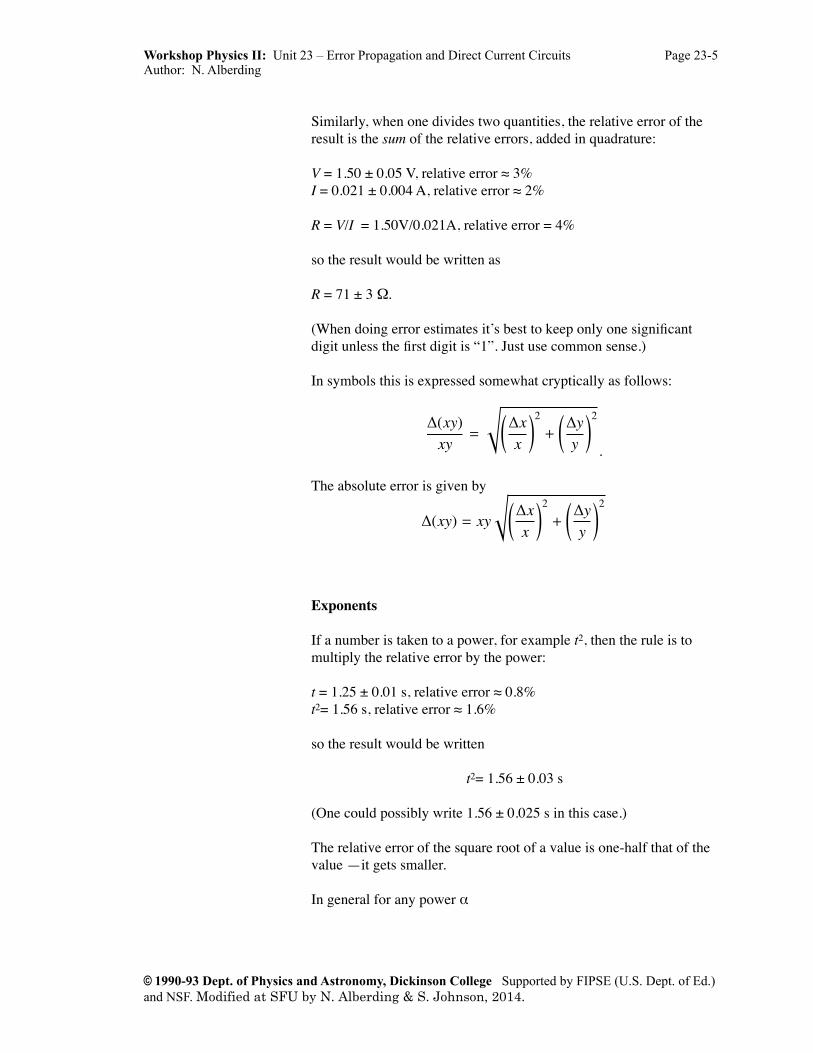
Similarly, when one divides two quantities, the relative error of the result is the sum of the relative errors, added in quadrature:

V = 1.50 ± 0.05 V, relative error ≈ 3%I = 0.021 ± 0.004 A, relative error ≈ 2%

R = V/I = 1.50V/0.021A, relative error = 4%

so the result would be written as

R = 71 ± 3 Ω.

(When doing error estimates it’s best to keep only one significant digit unless the first digit is “1”. Just use common sense.)

In symbols this is expressed somewhat cryptically as follows:

(xy)xy

=

s x

x

!2

+

y

y

!2

.

The absolute error is given by

(xy) = xy

s x

x

!2

+

y

y

!2

\Delta (xy) \over xy = \sqrt\left(\Delta x \over x \right)^2 + \left(\Delta y \over y \right)^2

Exponents

If a number is taken to a power, for example t2, then the rule is to multiply the relative error by the power:

t = 1.25 ± 0.01 s, relative error ≈ 0.8%t2= 1.56 s, relative error ≈ 1.6%

so the result would be written

t2= 1.56 ± 0.03 s

(One could possibly write 1.56 ± 0.025 s in this case.)

The relative error of the square root of a value is one-half that of the value —it gets smaller.

In general for any power α



(x)x= xx

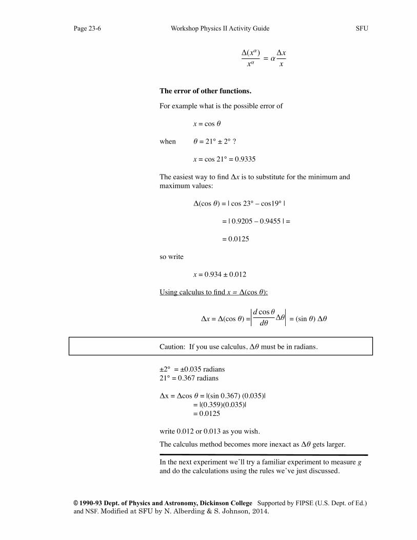
The error of other functions.

For example what is the possible error of

x = cos θ

when θ = 21° ± 2° ?

x = cos 21° = 0.9335

The easiest way to find Δx is to substitute for the minimum and maximum values:

Δ(cos θ) = | cos 23° – cos19° |

= | 0.9205 – 0.9455 | =

= 0.0125

so write

x = 0.934 ± 0.012

Using calculus to find x = Δ(cos θ):

Δx = Δ(cos θ) =d cos

d

= (sin θ) Δθ

Caution: If you use calculus, Δθ must be in radians.

±2° = ±0.035 radians21° = 0.367 radians

Δx = Δcos θ = |(sin 0.367) (0.035)| = |(0.359)(0.035)| = 0.0125

write 0.012 or 0.013 as you wish.

The calculus method becomes more inexact as Δθ gets larger.

In the next experiment we’ll try a familiar experiment to measure g and do the calculations using the rules we’ve just discussed.



• one ball • 5 stop watches • 1 tape measure • ladder or stool • method of designating the height of fall

Activity 23-1: Determining g by timing the fall of an object (This should be done as a class activity.)

Drop a ball from from a known height. Measure the height 5 times independently. (Different people who don’t know the results that the other got.) Then drop the ball from that height 5 times and measure it with 5 people armed with stopwatches. Tabulate the heights and times for the 5 trials in the following tables. Calculate the averages and standard deviations in each case. We can use a rule of thumb that for 4 or 5 trials the standard deviation is usually about 1/2 the range of the measurements.

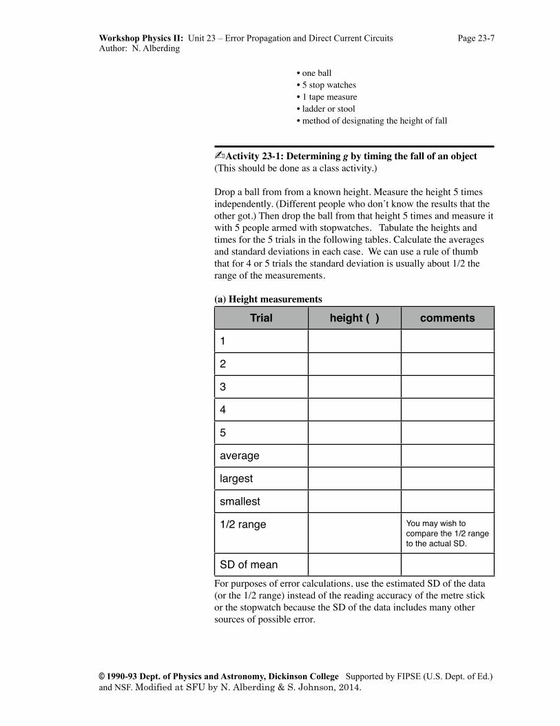
(a) Height measurements

Trial height ( ) comments

1

2

3

4

5

average

largest

smallest

1/2 range You may wish to compare the 1/2 range to the actual SD.

SD of meanFor purposes of error calculations, use the estimated SD of the data (or the 1/2 range) instead of the reading accuracy of the metre stick or the stopwatch because the SD of the data includes many other sources of possible error.





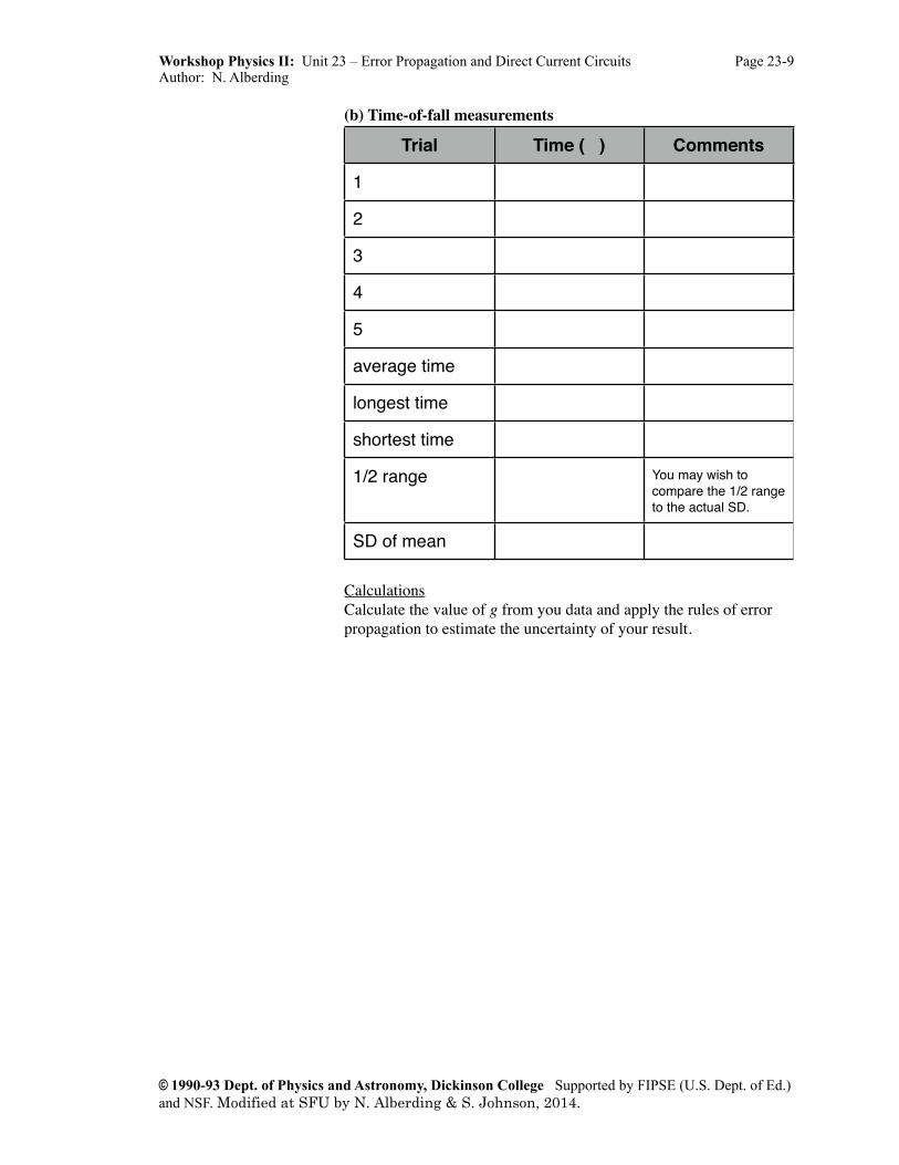
(b) Time-of-fall measurements

Trial Time ( ) Comments

1

2

3

4

5

average time

longest time

shortest time

1/2 range You may wish to compare the 1/2 range to the actual SD.

SD of mean

CalculationsCalculate the value of g from you data and apply the rules of error propagation to estimate the uncertainty of your result.



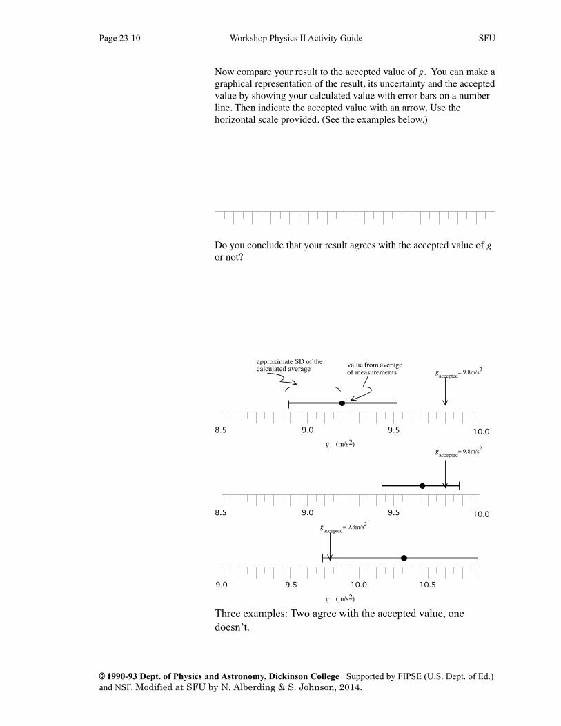
Now compare your result to the accepted value of g. You can make a graphical representation of the result, its uncertainty and the accepted value by showing your calculated value with error bars on a number line. Then indicate the accepted value with an arrow. Use the horizontal scale provided. (See the examples below.)

Do you conclude that your result agrees with the accepted value of g or not?

8.5 9.0 9.5 10.0

gaccepted

= 9.8m/s2value from average!of measurements

approximate SD of the calculated average

g (m/s2)

8.5 9.0 9.5 10.0

gaccepted

= 9.8m/s2

10.5g (m/s2)

gaccepted

= 9.8m/s2

9.0 10.09.5

Three examples: Two agree with the accepted value, one doesn’t.



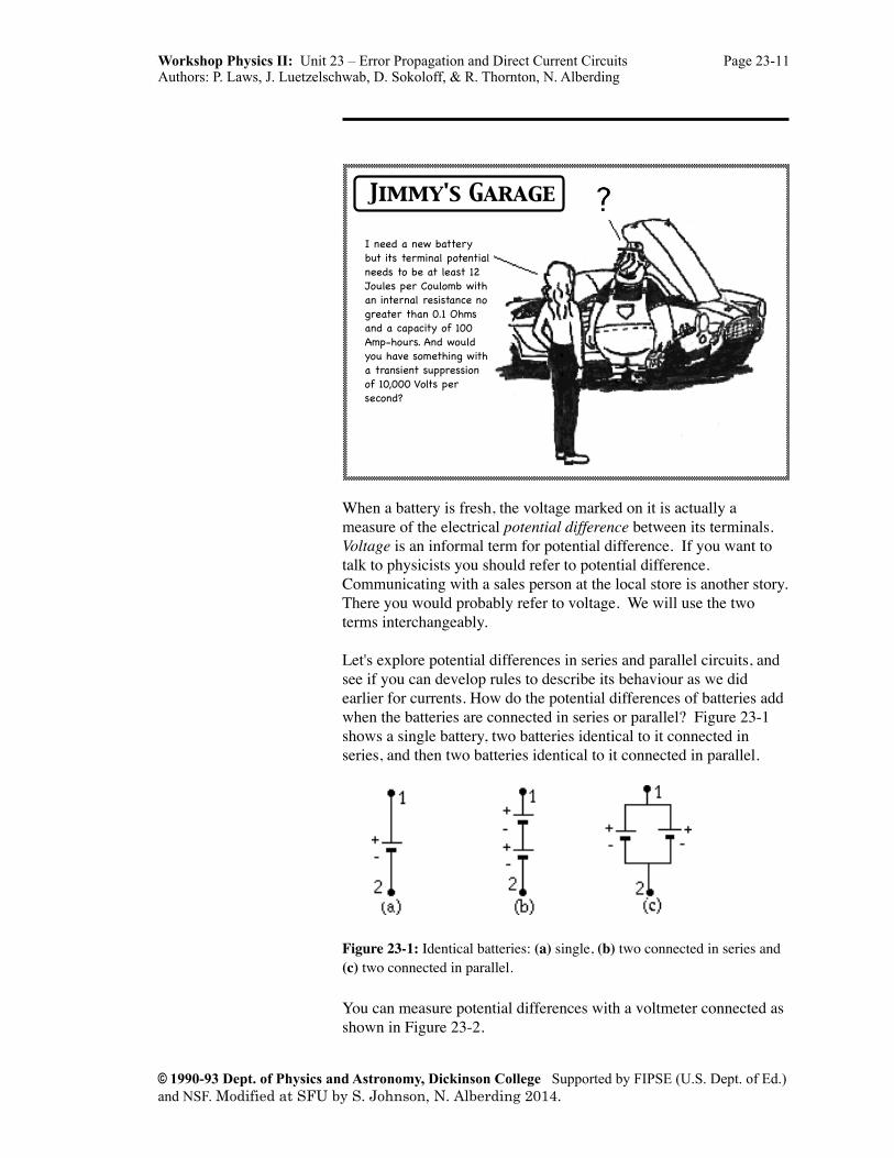
Jimmy's Garage

I need a new battery but its terminal potential needs to be at least 12 Joules per Coulomb with an internal resistance no greater than 0.1 Ohms and a capacity of 100 Amp-hours. And would you have something with a transient suppression of 10,000 Volts per second?

When a battery is fresh, the voltage marked on it is actually a measure of the electrical potential difference between its terminals. Voltage is an informal term for potential difference. If you want to talk to physicists you should refer to potential difference. Communicating with a sales person at the local store is another story. There you would probably refer to voltage. We will use the two terms interchangeably.

Let's explore potential differences in series and parallel circuits, and see if you can develop rules to describe its behaviour as we did earlier for currents. How do the potential differences of batteries add when the batteries are connected in series or parallel? Figure 23-1 shows a single battery, two batteries identical to it connected in series, and then two batteries identical to it connected in parallel.

Figure 23-1: Identical batteries: (a) single, (b) two connected in series and (c) two connected in parallel.

You can measure potential differences with a voltmeter connected as shown in Figure 23-2.

Workshop Physics II: Unit 23 – Error Propagation and Direct Current Circuits Page 23-11Authors: P. Laws, J. Luetzelschwab, D. Sokoloff, & R. Thornton, N. Alberding

© 1990-93 Dept. of Physics and Astronomy, Dickinson College Supported by FIPSE (U.S. Dept. of Ed.) and NSF. Modified at SFU by S. Johnson, N. Alberding 2014.

V

V

VV

V

Figure 23-2: Voltmeters connected to measure the potential difference across (a) a single battery, (b) a single battery and two batteries connected in series, and (c) a single battery and two batteries connected in parallel.

Activity 23-2: Combinations of Batteries(a) Predict the voltage for each combination of batteries in Fig 23-2. Write

you prediction beside the meter symbols.(b) Measure the voltages you predicted and write them below the predicted

values on the figure.

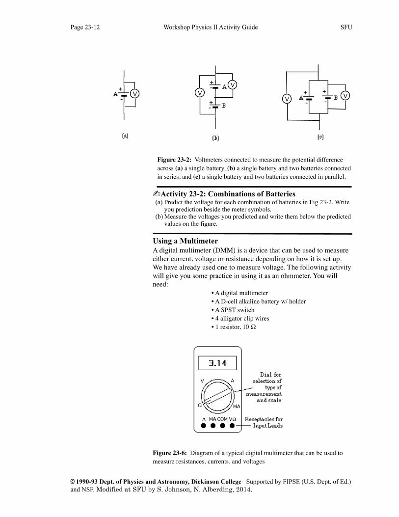
Using a MultimeterA digital multimeter (DMM) is a device that can be used to measure either current, voltage or resistance depending on how it is set up. We have already used one to measure voltage. The following activity will give you some practice in using it as an ohmmeter. You will need: • A digital multimeter • A D-cell alkaline battery w/ holder • A SPST switch • 4 alligator clip wires • 1 resistor, 10 Ω

VΩCOMMAA

Ω

V A

MA

Figure 23-6: Diagram of a typical digital multimeter that can be used to measure resistances, currents, and voltages


© 1990-93 Dept. of Physics and Astronomy, Dickinson College Supported by FIPSE (U.S. Dept. of Ed.) and NSF. Modified at SFU by S. Johnson, N. Alberding, 2014.

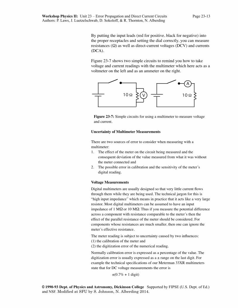
By putting the input leads (red for positive, black for negative) into the proper receptacles and setting the dial correctly, you can measure resistances (Ω) as well as direct-current voltages (DCV) and currents (DCA).

Figure 23-7 shows two simple circuits to remind you how to take voltage and current readings with the multimeter which here acts as a voltmeter on the left and as an ammeter on the right.

A

10 Ω 10 ΩV

Figure 23-7: Simple circuits for using a multimeter to measure voltage and current.

Uncertainty of Multimeter Measurements

There are two sources of error to consider when measuring with a multimeter:1. The effect of the meter on the circuit being measured and the

consequent deviation of the value measured from what it was without the meter connected and

2. The possible error in calibration and the sensitivity of the meter’s digital reading.

Voltage MeasurementsDigital multimeters are usually designed so that very little current flows through them while they are being used. The technical jargon for this is “high input impedance” which means in practice that it acts like a very large resistor. Most digital multimeters can be assumed to have an input impedance of 1 MΩ or 10 MΩ. Thus if you measure the potential difference across a component with resistance comparable to the meter’s then the effect of the parallel resistance of the meter should be considered. For components whose resistances are much smaller, then one can ignore the meter’s effective resistance.

The meter reading is subject to uncertainty caused by two influences: (1) the calibration of the meter and (2) the digitization error of the numerical reading.

Normally calibration error is expressed as a percentage of the value. The digitization error is usually expressed as a ± range on the last digit. For example the technical specifications of our Meterman 33XR multimeters state that for DC voltage measurements the error is

±(0.7% + 1 digit)



One calculates the uncertainty as 0.7% of the reading plus one digit in rightmost digit of the reading. For example

2.47 V would have an error of

±0.7% ⨉ 2.47 V = ±0.02 V added to ±0.01 Vresulting in a total error of ±0.03 V. (We do not add these two contributions in quadrature.)

Current MeasurementsCurrent measurements need to have the meter inserted in series with the circuit elements. Digital multimeters are apt to have a significant resistance compared to the other circuit elements, and the amount of resistance depends on the scale setting. For higher currents such as around 1 A the resistance could be a few ohms, but for milliampere ranges internal resistances could be as high as a kΩ. (Sometimes this is specified as “voltage burden” because there’s an unwanted voltage across the meter while it’s being used.) The result is that the meter causes the current being measured to be smaller than it would be without the meter.

The error on current measurements depends on the scale. For most scales it is listed as ±(1%+1digit) for the 33XR Meterman DMM

Resistance MeasurementsResistance measurements combine both voltage and current measurement. A meter has to provide a voltage and measure the current for that voltage and then presents the ratio of voltage to current as the resistance value. Because the meter has to provide an exact voltage across the component being measured it’s important to ensure that no other sources of voltage are connected which would interfere with the measurement. Similarly, the current from the meter must flow only through the component being measured. Therefore, the component must be disconnected from any other circuit element while the resistance is being measured. If the component is being tested in circuit, at least one end must be disconnected while measuring its resistance. While you’re measuring the resistance of something you must make sure that it is not connected to anything else. Even having your fingers touching the leads can cause an erroneous measurement due to the body’s resistance in parallel.

Because both voltage and current are involved in measuring resistance, it is normal that the uncertainty is somewhat more than that for voltage or current. Most scales have a listed error of ±(1%+4 digits) for the 33XR Meterman DMM.

AC/DCBoth current and voltage functions of a multimeter have alternating current and direct current scales. Most of our measurements should use the direct current setting. If you get reading of almost zero when you expect a larger



V

A

Ω

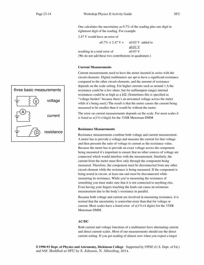
voltage

current

three basic measurements

resistance

value, then check if the meter is set on AC instead of DC. The specified error on AC measurements is typically larger than for DC measurements.

Other MeasurementsMany DMMs have the ability to make various other measurements depending on the model. Some can measure frequency, capacitance, temperature, inductance or transistor current amplification. These may be very useful in some situations, but the three basic measurements are essential and should be mastered first.

Activity 23-3: Using a Multimeter(a) Set up the circuit shown in Figure 23-7 with the switch open. Figure out what settings you need to use to measure the actual resistance of the "10Ω" resistor. Record your measured value with uncertainty below.

(b) Now close the switch and measure the actual resistance of the “10Ω” resistor again. Is your result different? (Do the two values agree within errors?) If so, what do you think is the cause of this difference?

Ohm’s Law: Relating Current, Potential Difference and ResistanceYou have already seen on several occasions that there is only a potential difference across a bulb when there is a current flowing through the bulb. In this activity we are going to use a resistor and compare its characteristics to a light bulb. Resistors are designed to have the same resistance value no matter how much current is passing through. How does the potential difference across a resistor depend on the current through it? In order to explore this, you will need the following:

• 2 digital multimeters • 4 D-cell alkaline batteries with holders •1 resistor, 47 Ω •1 light bulb, 6 V or larger •1 SPST switch



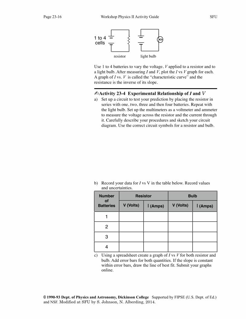
1 to 4 cells

resistor light bulb

Use 1 to 4 batteries to vary the voltage, V applied to a resistor and to a light bulb. After measuring I and V, plot the I vs V graph for each. A graph of I vs. V is called the “characteristic curve” and the resistance is the inverse of its slope.

Activity 23-4 Experimental Relationship of I and Va) Set up a circuit to test your prediction by placing the resistor in

series with one, two, three and then four batteries. Repeat with the light bulb. Set up the multimeters as a voltmeter and ammeter to measure the voltage across the resistor and the current through it. Carefully describe your procedures and sketch your circuit diagram. Use the correct circuit symbols for a resistor and bulb.

b) Record your data for I vs V in the table below. Record values and uncertainties.

Number of

Batteries

ResistorResistor BulbBulbNumber of

Batteries V (Volts) I (Amps) V (Volts) I (Amps)

1

2

3

4c) Using a spreadsheet create a graph of I vs V for both resistor and

bulb. Add error bars for both quantities. If the slope is constant within error bars, draw the line of best fit. Submit your graphs online.



Ohm's Law and ResistanceThe relationship between potential difference and current which you have observed for a resistor is known as Ohm's law. To put this law in its normal form, we must now define the quantity known as resistance. Resistance is defined by:

! ! ! R ! V/I

If potential difference (V ) is measured in volts and current (I) is measured in amperes, then the unit of resistance (R) is the ohm, which is usually represented by the Greek capital letter Ω, "omega."

Activity 23-5: Statement of Ohm's Lawa) State the mathematical relationship found in Activity 23-4 between potential difference and current for a resistor in terms of V, I, and R.

b) Based on your graph, what can you say about the value of R for a resistor — is it constant or does it change as the current through the resistor changes? Explain.

c) From the slope of your graph, what is the experimentally determined value of the resistance of your resistor in ohms? How does this agree with the rated value of the resistor?

d) Complete the famous pre-exam rhyme used by countless introductory

physics students throughout the English speaking world:

Twinkle, twinkle little star, V equals ______ times ______

Note: Some circuit elements do not obey Ohm's law. The definition for resistance is still the same, but, as with a light bulb, the resistance changes because of temperature changes resulting from the flow of current. Circuit elements which follow Ohm's law over a wide range of conditions--like resistors--are said to be ohmic, while circuit elements which do not--like a light bulb--are nonohmic.



SESSION TWO: KIRCHHOFF'S LAWS AND MULTI-LOOP CIRCUITS20 min

Resistance and Its MeasurementIn the series of observations you have been making with batteries and bulbs it is clear that electrical energy is being transferred to light and heat energy inside a bulb, so that even though all the current returns to the battery after flowing through the bulb, the charges have lost potential energy. We say that when electrical potential energy is lost in part of a circuit, such as it is in the bulb, it is because that part of the circuit offers resistance to the flow of electric current.

A battery causes charge to flow in a circuit. The electrical resistance to the flow of charge can be compared to the mechanical resistance offered by the pegs and the barrier in a mechanical model depicted by a ramp with balls travelling down it as described in Unit 22.

A light bulb is one kind of electrical resistance. Another common kind is provided by a resistor manufactured to provide a constant resistance in electrical circuits.

Resistors are the most standard sources of resistance used in electrical circuits for several reasons. A light bulb has a resistance which increases with temperature and current and thus doesn't make a good circuit element when quantitative attributes are important. The resistance of resistors doesn't vary with the amount of current passing through them. Resistors are inexpensive to manufacture and can be produced with low or high resistances.

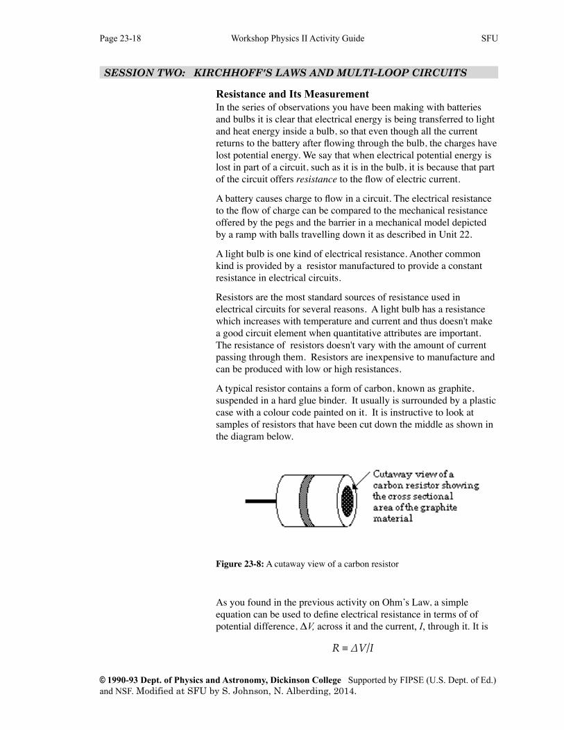
A typical resistor contains a form of carbon, known as graphite, suspended in a hard glue binder. It usually is surrounded by a plastic case with a colour code painted on it. It is instructive to look at samples of resistors that have been cut down the middle as shown in the diagram below.

Figure 23-8: A cutaway view of a carbon resistor

As you found in the previous activity on Ohm’s Law, a simple equation can be used to define electrical resistance in terms of of potential difference, ΔV, across it and the current, I, through it. It is

" " " R ! #V/I



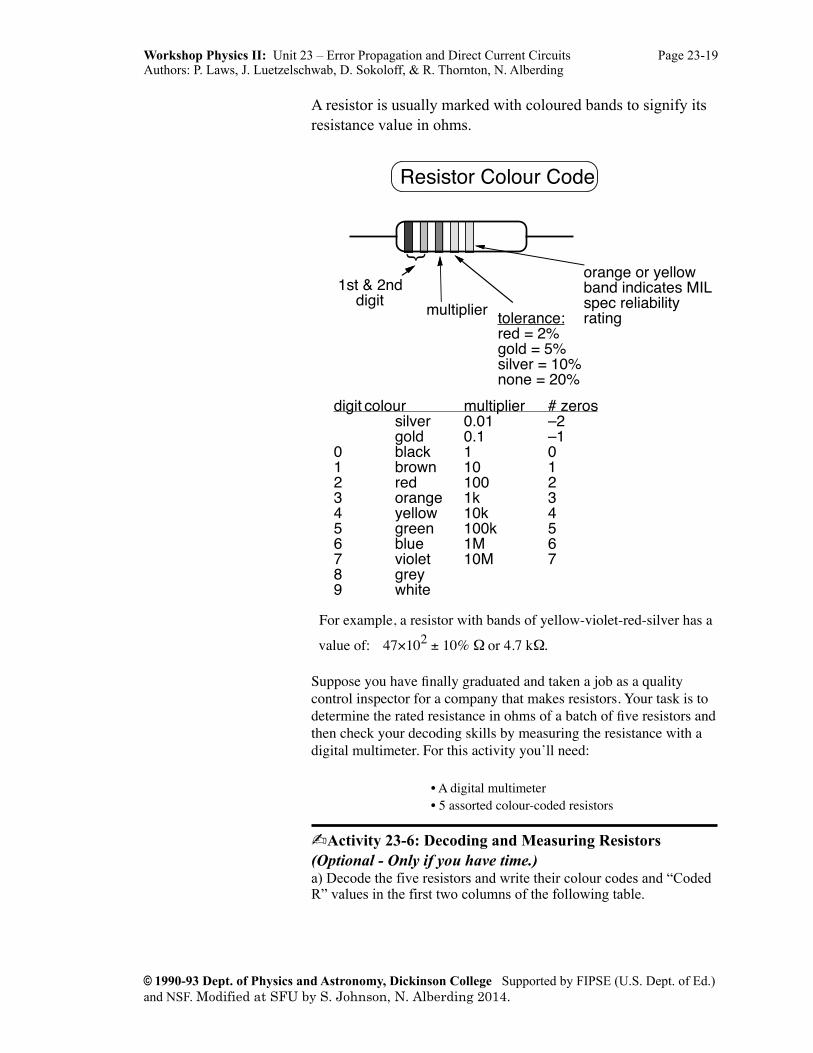
A resistor is usually marked with coloured bands to signify its resistance value in ohms.

Experiment EM2: DC Circuits and Measurements

EM2.11

Resistor Colour Code

1st & 2nd digit

multipliertolerance:red = 2%gold = 5%silver = 10%none = 20%

orange or yellow band indicates MIL spec reliability rating

digit colour multiplier # zerossilver 0.01 –2gold 0.1 –1

0 black 1 01 brown 10 12 red 100 23 orange 1k 34 yellow 10k 45 green 100k 56 blue 1M 67 violet 10M 78 grey9 white

For example, a resistor with bands of yellow-violet-red-silver has a

value of: 47×102 ± 10% Ω or 4.7 kΩ.

Suppose you have finally graduated and taken a job as a quality control inspector for a company that makes resistors. Your task is to determine the rated resistance in ohms of a batch of five resistors and then check your decoding skills by measuring the resistance with a digital multimeter. For this activity you’ll need:

• A digital multimeter • 5 assorted colour-coded resistors

Activity 23-6: Decoding and Measuring Resistors(Optional - Only if you have time.)a) Decode the five resistors and write their colour codes and “Coded R” values in the first two columns of the following table.



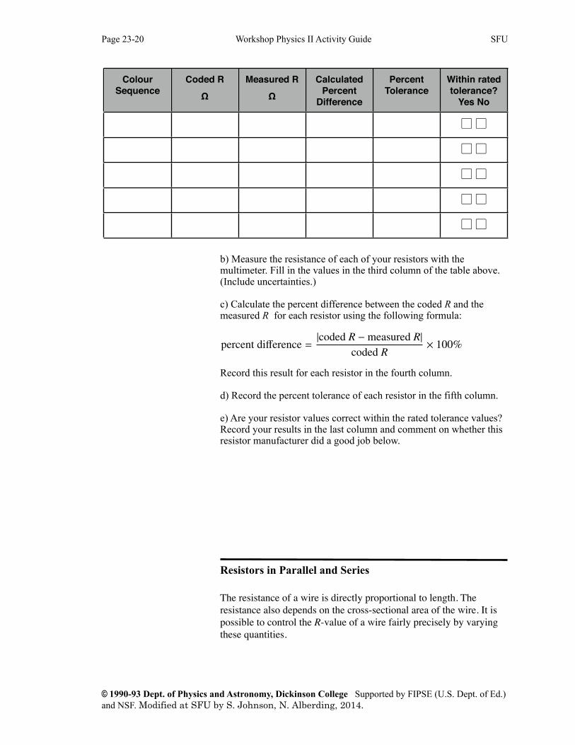
Colour Sequence

Coded RΩ

Measured RΩ

Calculated Percent

Difference

Percent Tolerance

Within rated tolerance?

Yes No

b) Measure the resistance of each of your resistors with the multimeter. Fill in the values in the third column of the table above. (Include uncertainties.)

c) Calculate the percent difference between the coded R and the measured R for each resistor using the following formula:

percent dierence =|coded R measured R|

coded R 100%

\rm percent~difference = |\rm coded~ R - \rm measured~R| \over \rm coded~R \times 100\%Record this result for each resistor in the fourth column.

d) Record the percent tolerance of each resistor in the fifth column.

e) Are your resistor values correct within the rated tolerance values? Record your results in the last column and comment on whether this resistor manufacturer did a good job below.

Resistors in Parallel and Series

The resistance of a wire is directly proportional to length. The resistance also depends on the cross-sectional area of the wire. It is possible to control the R-value of a wire fairly precisely by varying these quantities.



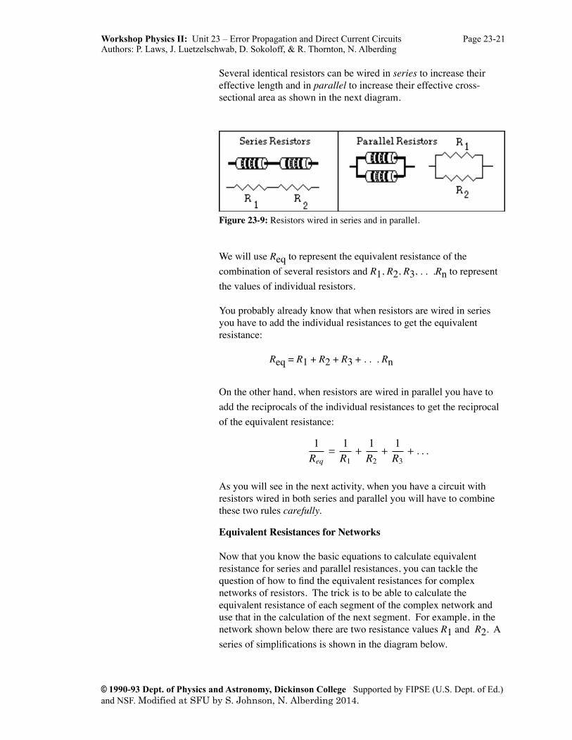
Several identical resistors can be wired in series to increase their effective length and in parallel to increase their effective cross-sectional area as shown in the next diagram.

Figure 23-9: Resistors wired in series and in parallel.

We will use Req to represent the equivalent resistance of the combination of several resistors and R1, R2, R3, . . .Rn to represent the values of individual resistors.

You probably already know that when resistors are wired in series you have to add the individual resistances to get the equivalent resistance:

Req = R1 + R2 + R3 + . . . Rn

On the other hand, when resistors are wired in parallel you have to add the reciprocals of the individual resistances to get the reciprocal of the equivalent resistance:

1Req=

1R1+

1R2+

1R3+ . . .

As you will see in the next activity, when you have a circuit with resistors wired in both series and parallel you will have to combine these two rules carefully.

25 minEquivalent Resistances for Networks

Now that you know the basic equations to calculate equivalent resistance for series and parallel resistances, you can tackle the question of how to find the equivalent resistances for complex networks of resistors. The trick is to be able to calculate the equivalent resistance of each segment of the complex network and use that in the calculation of the next segment. For example, in the network shown below there are two resistance values R1 and R2. A series of simplifications is shown in the diagram below.



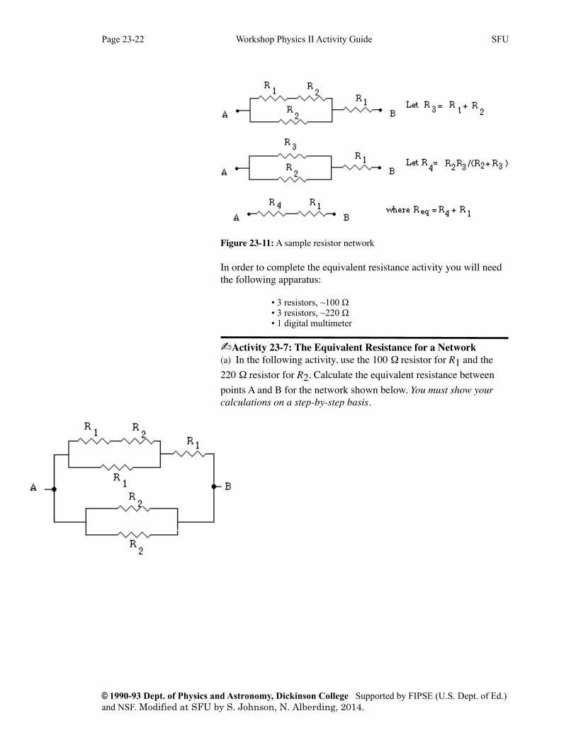
Figure 23-11: A sample resistor network

In order to complete the equivalent resistance activity you will need the following apparatus:

• 3 resistors, ~100 Ω • 3 resistors, ~220 Ω • 1 digital multimeter

Activity 23-7: The Equivalent Resistance for a Network(a) In the following activity, use the 100 Ω resistor for R1 and the 220 Ω resistor for R2. Calculate the equivalent resistance between points A and B for the network shown below. You must show your calculations on a step-by-step basis.



(b) Set up the network of resistors and check your calculation by measuring the equivalent resistance directly. (Hint: Build the circuit in stages and check the equivalent resistance for each stage.)

Calculated Value: Req = _________ Ω

Measured Value: Req = _________ Ω

50 minTheoretical Application of Kirchhoff's Laws Suppose we wish to calculate the currents in various branches of a circuit that has many components wired together in a complex array. In such circuits, simplification using series and parallel combinations is often impossible. Instead we can apply a formal set of rules known as Kirchhoff's laws to use in the analysis of current flow in circuits. These rules can be summarized as follows:

Kirchhoff’s Laws

1. Junction (or node ) Rule (based on charge conservation): The sum of all the currents entering any node or branch point of a circuit (i.e. where two or more wires merge) must equal the sum of all currents leaving the node.

2. Loop Rule (based on energy conservation): Around any closed loop in a circuit, the sum of all emfs (voltage gains provided by batteries or other power sources) and all the potential drops across resistors and other circuit elements must equal zero.

Steps for Applying Rules

1. Assign a current symbol to each branch of the circuit and label the current in each branch I1, I2, I3, etc.; then arbitrarily assign a direction to each current. (The direction chosen for the circuit for each branch doesn't matter. If you chose the "wrong" direction the value of the current will simply turn out to be negative.) Remember that the current flowing out of a battery is always the same as the current flowing into a battery.

2. Apply the loop rule to each of the loops by: (a) letting the potential drop across each resistor be the negative of the product of the resistance and the net current through that resistor (reverse the sign to “plus” if you are traversing a resistor in a direction opposite that of the current); (b) assigning a positive potential difference when the loop traverses from the – to the + terminal of a battery. (If you are going through a battery in the opposite direction assign a negative potential difference to the trip across the battery terminals.)



3. Find each of the junctions and apply the junction rule to it. You can place currents leaving the junction on one side of the equation and currents coming into the junction on the other side of the equation.

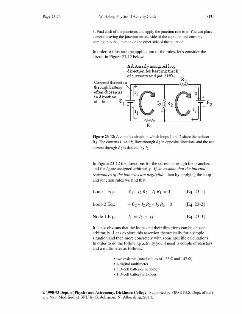
In order to illustrate the application of the rules, let's consider the circuit in Figure 23-12 below.

Figure 23-12: A complex circuit in which loops 1 and 2 share the resistor R2. The currents I1 and I3 flow through R2 in opposite directions and the net current through R2 is denoted by I2.

In Figure 23-12 the directions for the currents through the branches and for I2 are assigned arbitrarily. If we assume that the internal resistances of the batteries are negligible, then by applying the loop and junction rules we find that

Loop 1 Eq.: ε1 – I2 R2 – I1 R1 = 0 [Eq. 23-1]

Loop 2 Eq.: – ε2 + I2 R2 – I3 R3 = 0 [Eq. 23-2]

Node 1 Eq.: I1 = I2 + I3 [Eq. 23-3]

It is not obvious that the loops and their directions can be chosen arbitrarily. Let's explore this assertion theoretically for a simple situation and then more concretely with some specific calculations. In order to do the following activity you'll need a couple of resistors and a multimeter as follows:

• two resistors (rated values of ~22 Ω and ~47 Ω) • A digital multimeter • 3 D-cell batteries in holder • 1 D-cell battery in holder



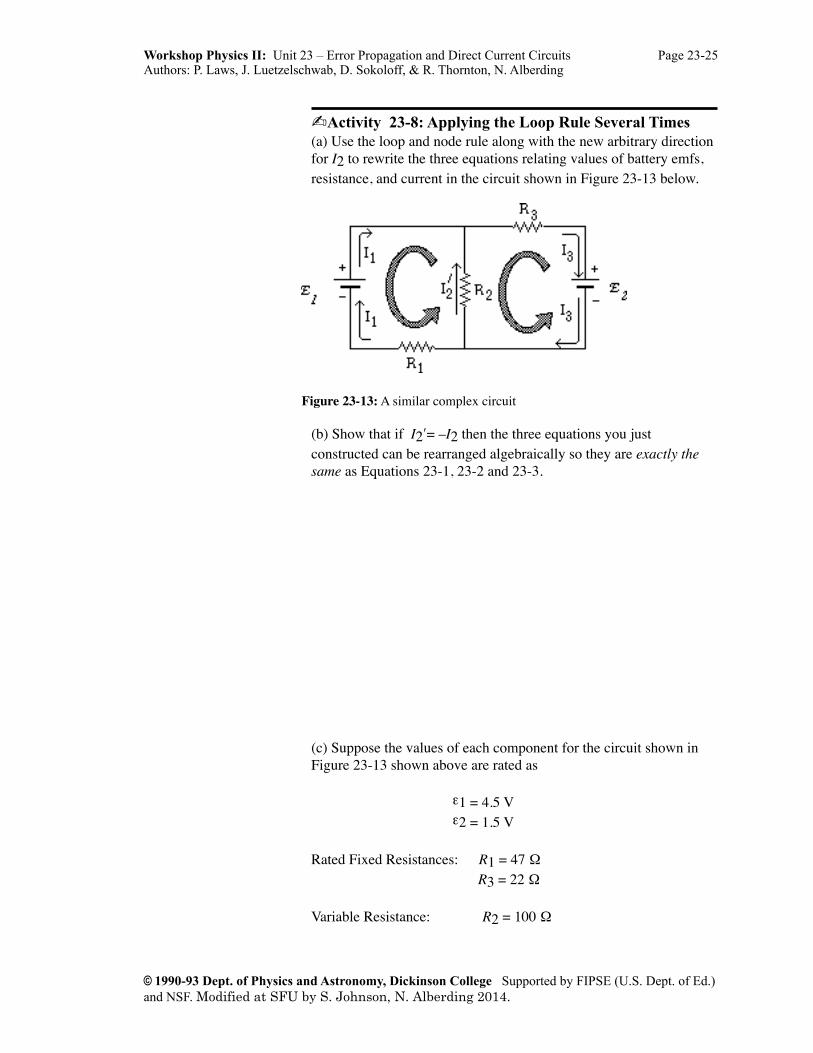
Activity 23-8: Applying the Loop Rule Several Times(a) Use the loop and node rule along with the new arbitrary direction for I2 to rewrite the three equations relating values of battery emfs, resistance, and current in the circuit shown in Figure 23-13 below.

Figure 23-13: A similar complex circuit

(b) Show that if I2ʹ′= –I2 then the three equations you just constructed can be rearranged algebraically so they are exactly the same as Equations 23-1, 23-2 and 23-3.

(c) Suppose the values of each component for the circuit shown in Figure 23-13 shown above are rated as

ε1 = 4.5 Vε2 = 1.5 V

Rated Fixed Resistances: R1 = 47 Ω R3 = 22 Ω

Variable Resistance: R2 = 100 Ω



1. Since you are going to test your theoretical results for Kirchhoff's law calculations for this circuit experimentally, you should measure the actual values of the two fixed resistors (rated at 47 Ω and 22 Ω) and the two battery voltages with a multimeter. List the results below.

Measured value of the battery emf rated at 4.5 V ε1 = ________

Measured value of the battery emf rated at 1.5 V ε2 = ________

Measured value of the resistor rated at 47 Ω: R1 = ________

Measured value of the resistor rated at 22 Ω: R3 = ________

2. Carefully rewrite Equations 23-1, 23-2 and 23-3 with the appropriate measured (not rated) values for emf and resistances substituted into them. Use 100 Ω for the value of R2 in your calculation. You will be setting a variable resistor to that value soon.

(d) Solve these three equations for the three unknowns I1, I2 and I3 in amps using one of the following methods: (1) substitution or (2) determinants.



(e) Show by substitution that your solutions actually satisfy the equations.

50 min



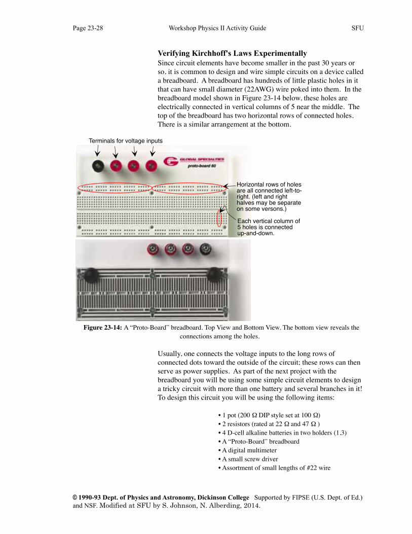
Verifying Kirchhoff's Laws Experimentally Since circuit elements have become smaller in the past 30 years or so, it is common to design and wire simple circuits on a device called a breadboard. A breadboard has hundreds of little plastic holes in it that can have small diameter (22AWG) wire poked into them. In the breadboard model shown in Figure 23-14 below, these holes are electrically connected in vertical columns of 5 near the middle. The top of the breadboard has two horizontal rows of connected holes. There is a similar arrangement at the bottom.

Horizontal rows of holes are all connected left-to-right. (left and right halves may be separate on some versons.)

Each vertical column of 5 holes is connected up-and-down.

Terminals for voltage inputs

Figure 23-14: A “Proto-Board” breadboard. Top View and Bottom View. The bottom view reveals the connections among the holes.

Usually, one connects the voltage inputs to the long rows of connected dots toward the outside of the circuit; these rows can then serve as power supplies. As part of the next project with the breadboard you will be using some simple circuit elements to design a tricky circuit with more than one battery and several branches in it! To design this circuit you will be using the following items:

• 1 pot (200 Ω DIP style set at 100 Ω) • 2 resistors (rated at 22 Ω and 47 Ω ) • 4 D-cell alkaline batteries in two holders (1,3) • A “Proto-Board” breadboard • A digital multimeter • A small screw driver • Assortment of small lengths of #22 wire



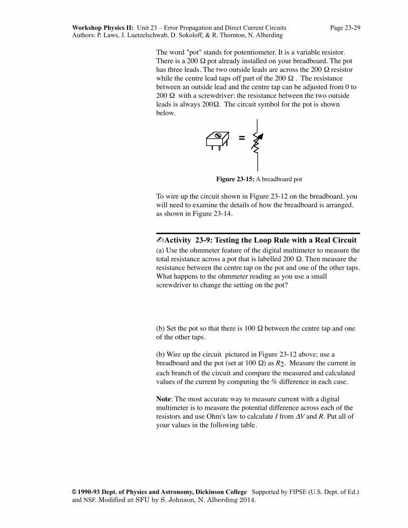
The word "pot" stands for potentiometer. It is a variable resistor. There is a 200 Ω pot already installed on your breadboard. The pot has three leads. The two outside leads are across the 200 Ω resistor while the centre lead taps off part of the 200 Ω . The resistance between an outside lead and the centre tap can be adjusted from 0 to 200 Ω with a screwdriver; the resistance between the two outside leads is always 200Ω. The circuit symbol for the pot is shown below.

Figure 23-15: A breadboard pot

To wire up the circuit shown in Figure 23-12 on the breadboard, you will need to examine the details of how the breadboard is arranged, as shown in Figure 23-14.

Activity 23-9: Testing the Loop Rule with a Real Circuit(a) Use the ohmmeter feature of the digital multimeter to measure the total resistance across a pot that is labelled 200 Ω. Then measure the resistance between the centre tap on the pot and one of the other taps. What happens to the ohmmeter reading as you use a small screwdriver to change the setting on the pot?

(b) Set the pot so that there is 100 Ω between the centre tap and one of the other taps.

(b) Wire up the circuit pictured in Figure 23-12 above; use a breadboard and the pot (set at 100 Ω) as R2. Measure the current in each branch of the circuit and compare the measured and calculated values of the current by computing the % difference in each case.

Note: The most accurate way to measure current with a digital multimeter is to measure the potential difference across each of the resistors and use Ohm's law to calculate I from ∆V and R. Put all of your values in the following table.



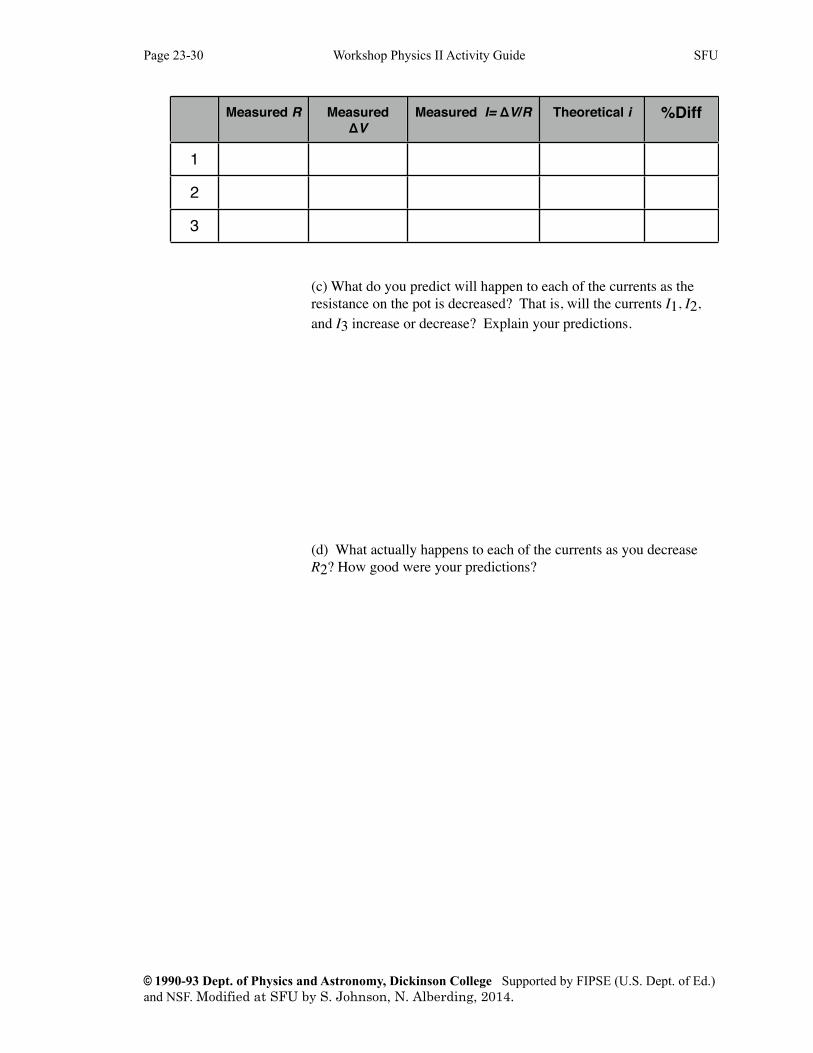
Measured R Measured ΔV

Measured I= ΔV/R Theoretical i %Diff

1

2

3

(c) What do you predict will happen to each of the currents as the resistance on the pot is decreased? That is, will the currents I1, I2, and I3 increase or decrease? Explain your predictions.

(d) What actually happens to each of the currents as you decrease R2? How good were your predictions?



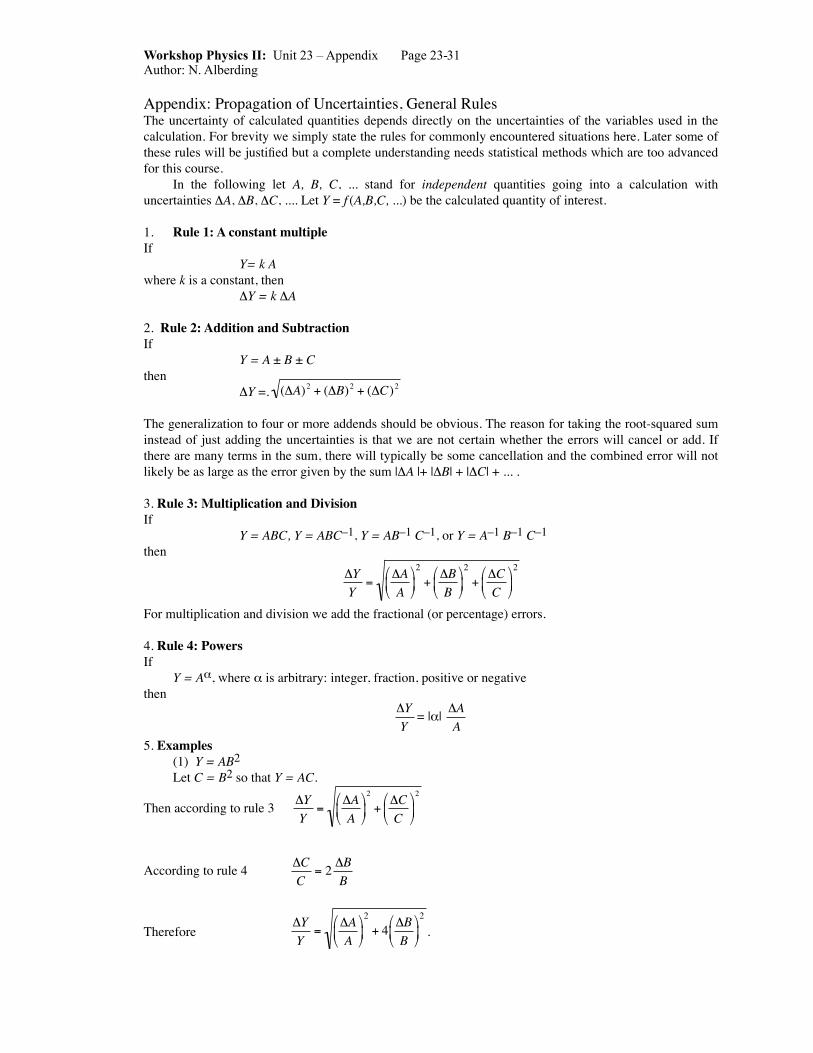
Appendix: Propagation of Uncertainties, General RulesThe uncertainty of calculated quantities depends directly on the uncertainties of the variables used in the calculation. For brevity we simply state the rules for commonly encountered situations here. Later some of these rules will be justified but a complete understanding needs statistical methods which are too advanced for this course. In the following let A, B, C, ... stand for independent quantities going into a calculation with uncertainties ΔA, ΔB, ΔC, .... Let Y = f (A,B,C, ...) be the calculated quantity of interest.

1. Rule 1: A constant multipleIf Y= k A where k is a constant, then ΔY = k ΔA

2. Rule 2: Addition and SubtractionIf Y = A ± B ± Cthen ΔY =.

€

(ΔA)2 + (ΔB)2 + (ΔC)2

The generalization to four or more addends should be obvious. The reason for taking the root-squared sum instead of just adding the uncertainties is that we are not certain whether the errors will cancel or add. If there are many terms in the sum, there will typically be some cancellation and the combined error will not likely be as large as the error given by the sum |ΔA |+ |ΔB| + |ΔC| + ... .

3. Rule 3: Multiplication and DivisionIf Y = ABC, Y = ABC–1, Y = AB–1 C–1, or Y = A–1 B–1 C–1then

€

ΔYY

=ΔAA

⎛

⎝ ⎜

⎞

⎠ ⎟ 2

+ΔBB

⎛

⎝ ⎜

⎞

⎠ ⎟ 2

+ΔCC

⎛

⎝ ⎜

⎞

⎠ ⎟ 2

For multiplication and division we add the fractional (or percentage) errors.

4. Rule 4: PowersIf Y = Aα, where α is arbitrary: integer, fraction, positive or negativethen

€

ΔYY

= |α|

€

ΔAA

5. Examples (1) Y = AB2 Let C = B2 so that Y = AC.

Then according to rule 3

€

ΔYY

=ΔAA

⎛

⎝ ⎜

⎞

⎠ ⎟ 2

+ΔCC

⎛

⎝ ⎜

⎞

⎠ ⎟ 2

According to rule 4

€

ΔCC

= 2 ΔBB

Therefore

€

ΔYY

=ΔAA

⎛

⎝ ⎜

⎞

⎠ ⎟ 2

+ 4 ΔBB

⎛

⎝ ⎜

⎞

⎠ ⎟ 2

.

Workshop Physics II: Unit 23 – Appendix Page 23-31Author: N. Alberding

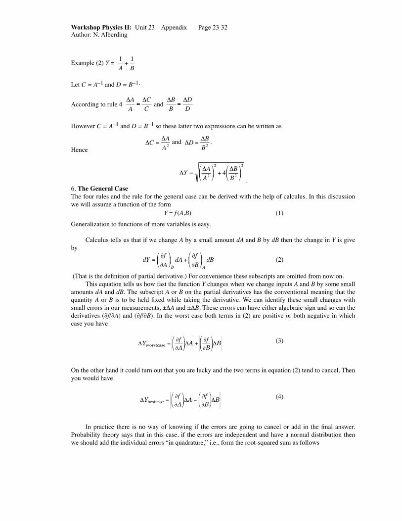
Example (2) Y =

€

1A

+1B

Let C = A–1 and D = B–1.

According to rule 4

€

ΔAA

=ΔCC

and

€

ΔBB

=ΔDD

However C = A–1 and D = B–1 so these latter two expressions can be written as

€

ΔC =ΔAA2

and

€

ΔD =ΔBB2

.Hence

€

ΔY =ΔAA2

⎛

⎝ ⎜

⎞

⎠ ⎟ 2

+ 4 ΔBB2

⎛

⎝ ⎜

⎞

⎠ ⎟ 2

.6. The General CaseThe four rules and the rule for the general case can be derived with the help of calculus. In this discussion we will assume a function of the form Y = f (A,B) (1)

Generalization to functions of more variables is easy.

Calculus tells us that if we change A by a small amount dA and B by dB then the change in Y is give by

€

dY =∂f∂A⎛

⎝ ⎜

⎞

⎠ ⎟ BdA +

∂f∂B⎛

⎝ ⎜

⎞

⎠ ⎟ AdB

(2)

(That is the definition of partial derivative.) For convenience these subscripts are omitted from now on. This equation tells us how fast the function Y changes when we change inputs A and B by some small amounts dA and dB. The subscript A or B on the partial derivatives has the conventional meaning that the quantity A or B is to be held fixed while taking the derivative. We can identify these small changes with small errors in our measurements, ±ΔA and ±ΔB. These errors can have either algebraic sign and so can the derivatives (∂f/∂A) and (∂f/∂B). In the worst case both terms in (2) are positive or both negative in which case you have

€

ΔYworstcase =∂f∂A

⎛

⎝ ⎜

⎞

⎠ ⎟ ΔA +

∂f∂B

⎛

⎝ ⎜

⎞

⎠ ⎟ ΔB (3)

On the other hand it could turn out that you are lucky and the two terms in equation (2) tend to cancel. Then you would have

€

ΔYbestcase =∂f∂A

⎛

⎝ ⎜

⎞

⎠ ⎟ ΔA −

∂f∂B

⎛

⎝ ⎜

⎞

⎠ ⎟ ΔB (4)

In practice there is no way of knowing if the errors are going to cancel or add in the final answer. Probability theory says that in this case, if the errors are independent and have a normal distribution then we should add the individual errors “in quadrature,” i.e., form the root-squared sum as follows


€

ΔY =∂f∂A⎛

⎝ ⎜

⎞

⎠ ⎟ ΔA

⎛

⎝ ⎜

⎞

⎠ ⎟

2

+∂f∂B⎛

⎝ ⎜

⎞

⎠ ⎟ ΔB

⎛

⎝ ⎜

⎞

⎠ ⎟

2

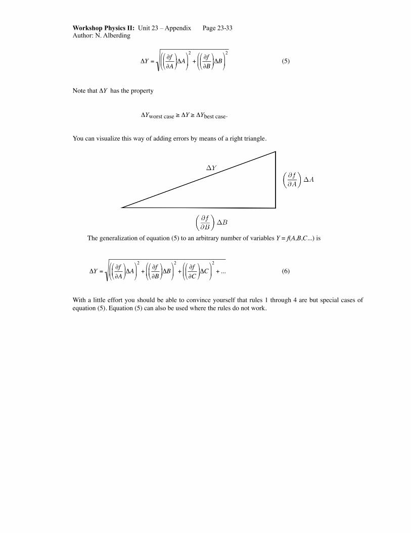
(5)

Note that ΔY has the property

ΔYworst case ≥ ΔY ≥ ΔYbest case.

You can visualize this way of adding errors by means of a right triangle.

The generalization of equation (5) to an arbitrary number of variables Y = f(A,B,C...) is

€

ΔY =∂f∂A⎛

⎝ ⎜

⎞

⎠ ⎟ ΔA

⎛

⎝ ⎜

⎞

⎠ ⎟

2

+∂f∂B⎛

⎝ ⎜

⎞

⎠ ⎟ ΔB

⎛

⎝ ⎜

⎞

⎠ ⎟

2

+∂f∂C⎛

⎝ ⎜

⎞

⎠ ⎟ ΔC

⎛

⎝ ⎜

⎞

⎠ ⎟

2

+ ... (6)

With a little effort you should be able to convince yourself that rules 1 through 4 are but special cases of equation (5). Equation (5) can also be used where the rules do not work.


Documents

Unit 23: ERROR PROPAGATION, DIRECT CURRENT CIRCUITS