Embed Size (px)
Citation preview

United States Natural Resources 11 Campus Boulevard Department of Conservation Suite 200 Agriculture Service Newtown Square, PA 19073 Subject: SOI – Geophysical Field Assistance Date: 14 July 2003 To: Dr. Heidi Hadley
Hydrologist USDI, Bureau of Land Management Utah State Office P.O. Box 45155 Salt Lake City, UT 84145-0155
Purpose: The purpose of this investigation was to use electromagnetic induction to provide detailed soil information and maps for a transit sources salinity loading study along the upper reaches of the San Rafael River, Colorado River Basin, Utah. Participants: Janis Boettinger, Assoc. Professor, Utah State Univ., Logan, UT Jim Brown, Range Management Specialist, USDA-NRCS, Roosevelt, UT Suzann Kienast-Brown, Soil Scientist, USDA-NRCS, Logan, UT Jim Doolittle, Research Soil Scientist, USDA-NRCS-NSSC, Newtown Square, PA Travis James, Resource Conservationist, USDA-NRCS, Salt Lake City, UT John Lawley, Research Associate, Utah State Univ., Logan, UT Jeremy Maycock, Soil Conservationist, USDA-NRCS, Richfield, UT Shawn Nield, Soil Scientist, USDA-NRCS, Logan, UT Victor Parslow, Soil Scientist, USDA-NRCS, Richfield, UT Gary Rheoden, Area Resource Conservationist, USDA-NRCS, Price, UT Leland Sasser, Soil Scientist, USDA-NRCS, Price, UT Jim Spencer, Wildlife Biologist, USDA-NRCS, Roosevelt, UT Wes Tuttle, Soil Scientist (Geophysical), USDA-NRCS-NSSC, Wilkesboro, NC Ed Whicker, Civil Engineer, USDA-NRCS, Roosevelt, UT Activities: All activities were completed during the period of 24 to 27 June 2003. Results:
1. Although data and survey sites were sparse, an analysis of variance revealed significant differences in ECa among the different formations (Carmel, Entrada, Curtis, Summerville, Morrison, and Mancos) and soils. For ECa measurements collected in both dipole orientations, the Mancos and Morrison formations have the largest means and were the most variable; the Entrada and Curtis formations have the lowest means and were among the least variable. Results suggest that EMI can be used in the San Rafael Swell to distinguish different soils and geologic formations.
2. At all three detailed survey sites, linear or plume-like features of high (>80 mS/m) apparent conductivity were
observed. In general, ECa in excess of 40 to 80 mS/m are indicative of high concentrations of soluble salts. Generally, in these areas, the contribution of salts far outweighs the contribution of moisture, clay content, clay type, and cation exchange capacity on apparent conductivity. The location and orientation of these lines or plume-like features of higher ECa suggest seepage from adjoining fans and bedrock escarpments. Salt-bearing waters appear to drain from the base of some bedrock escarpments. These waters leave high

2concentrations of residual salts in the soil near the bases of fans and escarpments. While high concentrations of soluble salts occur in many of the geologic formations within the San Rafael River Basin, no upland site contained as high or as extensive an area of high apparent conductivity as the areas investigated along the floodplain of the San Rafael River.
3. EMI appears to be an appropriate reconnaissance tool for determining transit mechanisms and sources of salt
loading within the San Rafael River Basin.
4. Maps of apparent conductivity contained in this report for the three survey sites along the San Rafael River will hopefully aid investigators to better understand the hydrogeology of these sites and to locate additional piezometers. CD’s of the data collected in this study have been prepared and forwarded to Heidi Hadley and Shawn Nield under a separate cover letter. In addition shape files of the two-dimensional simulations found in this report have been forwarded to Shawn Nield for his graduate research work.
5. The National Soil Survey Center’s soil salinity probe (Martek model 132-soil; serial number 268;
AG0002361060) was loaned to Shawn Nield and the Utah Soil Survey Staff to help complete the objectives of this investigation.
It was Wes Tuttle’s and my privilege to work with you and the Utah NRCS Soil Survey Staff. With kind regards, James A. Doolittle Research Soil Scientist National Soil Survey Center cc: B. Ahrens, Director, USDA-NRCS, National Soil Survey Center, Federal Building, Room 152,100 Centennial Mall
North, Lincoln, NE 68508-3866 J. Boettinger, Associate Professor, Plants, Soils, and Biometeorology, Utah State University, 4820 Old Main Hill, Ag.
Sci. Bldg., Room 354, Logan, UT 84322-4820 W. Broderson, State Soil Scientist, USDA-NRCS, PO Box 11350, Salt Lake City, UT 84147-0350 W. Maresch, Acting Director of Soils Survey Division, USDA-NRCS, Room 4250 South Building, 14th &
Independence Ave. SW, Washington, DC 20250 S. Nield, Soil Scientist, USDA-NRCS, North Logan Service Center, 1860 N 100 E, North Logan, UT 84341-1784 C. Olson, National Leader, Soil Investigation Staff, USDA-NRCS, National Soil Survey Center, Federal Building,
Room 152,100 Centennial Mall North, Lincoln, NE 68508-3866 L. Sasser, Soil Scientist, USDA-NRCS, Price Service Center, 350 N 400 E. Price, UT 84501-2571 W. Tuttle, Soil Scientist (Geophysical), USDA-NRCS-NSSC, P.O. Box 974, Federal Building, Room 206, 207 West
Main Street, Wilkesboro, NC 28697

3 Background: The San Rafael River is a major tributary to the Green River that flows into the Colorado River. The San Rafael River is located in the Colorado Plateau physiographic province and is underlain by several different geologic formations. Several of these formations contain large amounts of calcium, sodium, selenium, and magnesium compounds, which have created high levels of total dissolved solids and salinity problems along the San Rafael River (Hadley, 2002). The dissolution of soluble salts in the soil and substrata is a major source of the salt loading within the San Rafael River basins. Law and Hornsby (1982) reported that 52 percent of the salinity loading that occurs in the upper Colorado River Basin is from naturally diffused and non-irrigated sources. In order to control salt loading along the San Rafael and other rivers in the Colorado River Basin, knowledge is needed of surface runoff or groundwater inflow into streams. A purpose of this study is to develop and test methodologies for determining major transit mechanisms and sources of salt loads that reach the San Rafael River. Electromagnetic induction (EMI) was used to characterize several formations and survey sites, and to map areas of higher salt concentrations associated with surface runoff or groundwater inflow. Electromagnetic Induction (EMI): EMI uses electromagnetic energy to measure the apparent conductivity of earthen materials. Apparent conductivity is a weighted, average conductivity measurement for a column of earthen materials to a specific depth (Greenhouse and Slaine, 1983). Interpretations of EMI data are based on the identification of spatial patterns within data sets. Though seldom diagnostic in themselves, lateral and vertical variations in apparent conductivity have been used to infer changes in soils and geologic materials. Variations in apparent conductivity are produced by changes in the electrical conductivity of earthen materials. The electrical conductivity of earthen materials will increase with increases in soluble salt, water, and clay contents (Kachanoski et al., 1988; Rhoades et al., 1976). The electrical conductivity of soils is influenced by the type and concentration of ions in solution, the amount and type of clays in the soil matrix, the volumetric water content, and the temperature and phase of the soil water (McNeill, 1980b). In rocks, electrical conductivity is affected by the porosity, permeability, and clay content, as well as by the dissolved-solids concentration of the water within the rocks. In areas of saline soils, 65 to 70 percent of the variance in apparent conductivity can be explained by changes in the concentration of soluble salts alone (Williams and Baker, 1982). Moderate to high correlations have been found between apparent conductivity (ECa) and saturated paste extract (ECe), the most accepted and accurate method of determining soil salinity (de Jong, 1979; Williams and Baker, 1982; and Wollenhaupt et al., 1986). Studies have demonstrated that EMI can provide reasonably accurate estimates of soil salinity (Williams and Baker, 1982; van der Lelij, 1983; Diaz and Herrero, 1992). Different salts have different mobility’s and electrical conductivities. Cook and Williams (1998) noted that NaCl, CaCl2, MgCl2, and Na2SO4 have similar electrical conductivity at equivalent concentration, but MgSO4, CaSO4, and NaHCO3 have lower conductivities at equivalent salt concentrations. Equipment: Electromagnetic induction instruments used in this study were the EM31 and EM38DD meters. These meters are portable and need only one person to operate. No ground contact is required with these instruments. These meters measured the apparent conductivity of the underlying earthen materials. Values of apparent conductivity are expressed in milliSiemens per meter (mS/m). For each meter, lateral resolution is approximately equal to the intercoil spacing. Geonics Limited manufactures the EM31 and EM38DD meters.1 McNeill (1980a) has described the principles of operation for the EM31 meter. The EM31 meter has a 3.66-m intercoil spacing and operates at a frequency of 9,810 Hz. When placed on the soil surface, the EM31 meter has theoretical penetration depths of about 3.0 and 6.0 meters in the horizontal and vertical dipole orientations, respectively (McNeill, 1980a).
1 Trade names are used to provide specific information. Their mention does not constitute endorsement by USDA-NRCS.

4Geonics Limited (2000) describes the operating procedures for the EM38DD meter. The EM38DD meter has a 1-m intercoil spacing and operates at a frequency of 14,600 Hz. When placed on the soil surface, it has effective penetration depths of about 0.75 and 1.5 m in the horizontal and vertical dipole orientations, respectively (Geonics Limited, 2000). The EM38DD meter consists of two EM38 meters bolted together and electronically coupled. One meter acts as a master unit (meter that is positioned in the vertical dipole orientation and having both transmitter and receiver activated) and one meter acts as a slave unit (meter that is positioned in the horizontal dipole orientation with only the receiver switched on). The Geonics DAS70 Data Acquisition System was used to record and store both EMI and GPS data. 2 The acquisition system consists of the EM38DD or EM31 meter, an Allegro field computer, and a Trimble AG114 GPS receiver. With the logging system, the meters are keypad operated and measurements can either be automatically or manually triggered. To help summarize the results of this study, the SURFER for Windows (version 8) program, developed by Golden Software, Inc., was used to construct two-dimensional simulations and shape files. 2 Grids were created using kriging methods with an octant search. Field Procedures: Each meter was operated with the DAS70 data acquisition system and all measurements were georeferenced with the Trimble AG114 GPS. Each meter was operated in the continuous mode with measurements recorded at a 1-sec interval. The meters were generally orientated with their long axis parallel to the direction of traverse. The EM38DD was held about 2 inches above the ground surface. The EM31 meter was held at hip height and surveys were carried out in the vertical dipole orientation. Walking at a fairly uniform pace across a specified unit completed an EMI survey and file. Grid surveys were completed at Fuller Bottom, Hambrick Bottom, and Entrada unit. Walking at a fairly uniform pace in a back and forth pattern across each survey area with an EMI instrument completed a grid survey. At several sites, negative values of apparent conductivity were recorded with the EM38DD meter. Prior to plotting, the EM38DD data for each of these sites were zero adjusted. Zero adjustment results in the lowest recorded measurement being made equal to zero and all other data being adjusted upwards by the same number used to make the lowest measurement equal to zero. Results: Lithologic Investigations: The headwaters of the San Rafael River cross (from youngest to oldest) the Mancos, Morrison, Summerville, Curtis, Entrada, and Carmel formations. EMI integrates the bulk physical and chemical properties of earthen materials within a defined depth into a single value. As a consequence, measurements have been associated with changes in geologic formations and lithology (McNeill, 1980b, Palacky, 1987; Sinha et al., 1985; and Zalasiewicz et al., 1985). The electrical conductivity of soil and geological materials varies over several orders of magnitude. For each soil and geologic material, intrinsic physical and chemical properties, as well as temporal variations in water content and temperature, result in a unique or characteristic range of apparent conductivity. In some investigations, EMI has provided useful geological information. In other investigations, interpretations are more ambiguous because of the interplay of several factors (moisture, clays, salts), which resulted in similar responses over different and seemingly contrasting lithologies. A study was conducted to determine whether distinct EMI responses were obtainable over the different geologic formations and representative upland soils within the San Rafael River Basin. Random traverses were conducted with the EM38DD and EM31 meters across upland areas of each lithologic unit. Table 1 lists the taxonomic classifications of the soil most commonly associated with six formations.
2 Trade names are used to provide specific information. Their mention does not constitute endorsement by USDA-NRCS.
5Table 1. Taxonomic Classification of Soils associated with distinct geologic formations within the
San Rafael River Basin Soil Classification Formation.
Chipeta Clayey, mixed, active, calcareous, mesic, shallow Typic Torriorthents Mancos Farb Loamy, mixed, superactive, calcareous, mesic Lithic Torriorthents Curtis Hadden Fine-loamy, mixed, superactive, mesic Typic Natrargids Morrison Hanksville Fine, mixed, active, calcareous, mesic Typic Torriorthents Mancos Moffat Coarse-loamy, mixed, superactive, mesic Typic Haplocalcids Entrada Mussentuchit Coarse-loamy, gypsic, mesic Typic Calcigypsids Carmel Robroost Coarse-loamy, mixed, active, mesic Typic Calcigypsids Carmel Sandbench Sandy, mixed, mesic Typic Haplocalcids Curtis Shalet Loamy, mixed, active, calcareous, mesic, shallow Typic Torriorthents Summerville
Carmel Formation: The Jurassic Carmel formation contains gypsum-bearing siltstone and shales. On upland areas of the Carmel formation, the dominant soils are the gypsiferous, coarse-loamy, well drained Mussentuchit and Robroost series. The moderately deep Mussentuchit and very deep Robroost soils formed in residuum weathered mainly from soft gypsiferous sandstone and shale. Figure 1 shows the responses of the EM38 meter over a representative upland area of the Carmel formation. Higher values of apparent conductivity were associated with dry washes. The washes had visible salt flecks on the surface and contained higher levels of soluble salts, which contributed to the higher apparent conductivity. At all observation points (N=94), measurements obtained in the deeper-sensing vertical dipole orientation were higher than those obtained in the shallower-sensing horizontal dipole orientation. This relationship is associated with drier surface conditions and higher salt concentrations at lower soil depths. In this area of the Carmel formation, with the EM38DD meter, apparent conductivity increased and became slightly more variable with increasing depth. In the shallower-sensing, horizontal dipole orientation, apparent conductivity averaged about 10.2 mS/m with a standard deviation of about 5.5 mS/m. One-half the observations had values of apparent conductivity between about 6.1 and 14.8 mS/m. In the deeper-sensing, vertical dipole orientation, apparent conductivity averaged about 19.7 mS/m with a standard deviation of about 6.9 mS/m. One-half the observations had values of apparent conductivity between about 14.0 and 25.4 mS/m.
Figure 1. Response of EM38DD meter over the Carmel formation.
0
5
10
15
20
25
30
35
40
1 10 19 28 37 46 55 64 73 82 91
Station
Ap
par
ent
Co
nd
uct
ivit
y (m
S/m
)
EM38DD-V
EM38DD-H

6A similar trend was measured with the deeper-sensing EM31 meter operated in the vertical dipole orientation. Apparent conductivity averaged about 21.3 mS/m with a standard deviation of 7.2 mS/m. One-half the observations had values of apparent conductivity between 18.0 and 25.5 mS/m. Although at this and other upland sites, the soils were mostly nonsaline (saline soils typically have ECa > 40 to 80 mS/m), the meters produced normal “salt profiles” indicating that ECa and presumably salts increase rapidly with depth (Corwin and Rhoades, 1984 and 1990). The increased conductivity with increasing depth at this site was attributed to higher gypsum and calcium-carbonate contents at lower soil depths. However, the relatively moderate to low ECa on these well-drained, coarse-loamy, gypsiferous soils do not suggest the presence of saline soils and the effect of high concentrations of gypsum on EMI response appears minimal. Entrada formation: The Jurassic Entrada formation consists of an upper member of sandstone and lower members of less resistant siltstone and mudstone (Chronic, 1998). The Entrada formation is characterized by the coarse-loamy, well-drained Moffat series. The very deep Moffat soil formed in eolian and alluvial sediments. Depths to calcic horizon ranges from 3 to 20 inches. Figure 2 shows the responses of the EM38DD meter over a representative area of the Entrada formation. At all observation points (N=127), measurements obtained in the deeper-sensing vertical dipole orientation were higher than those obtained in the shallower-sensing horizontal dipole orientation.
Figure 2. Response of EM38DD meter over the Entrada formation. With the EM38DD meter, apparent conductivity increased and became slightly more variable with increasing depth. In the shallower-sensing, horizontal dipole orientation, apparent conductivity averaged 3.4 mS/m with a standard deviation of 1.6 mS/m. One-half the observations had values of apparent conductivity between 3.6 and 4.4 mS/m. In the deeper-sensing, vertical dipole orientation, apparent conductivity averaged 10.6 mS/m with a standard deviation of 1.1 mS/m. One-half the observations had values of apparent conductivity between 10.5 and 11.3 mS/m. The increased conductivity with increasing depth was attributed to greater moisture, soluble salt, and clay contents at lower soil depths. Unfortunately, data collected with the EM31 meter over the Entrada formation was lost. In general, apparent conductivity measured with the EM38DD meter was low over the Entrada formation. Compared with the Carmel formation, ECa was noticeably lower and less variable in both dipole orientations over the Entrada formation. Soils at both sites were well drained, calcareous, and coarse-loamy. However, soils at the Carmel site (Mussentuchit and Robroost soils) were gypsiferous. Differences evident in figures 1 and 2, and in the averaged ECa between the Carmel (19.6 and 10.2 mS/m in the vertical and horizontal dipole orientations, respectively) and the
0
5
10
15
20
25
30
1 21 41 61 81 101 121
Station
Ap
par
ent
Co
nd
uct
ivit
y (m
S/m
)
EM38DD-V
EM38DD-H

7Entrada (10.6 and 3.4 mS/m in the vertical and horizontal dipole orientations, respectively) are tentatively attributed to differences in the gypsum contents of these soils. Curtis formation: The Jurassic Curtis formation consists of pale greenish marine sandstones, mudstone and shales. Curtis contains beds and nodules of gypsum and anhydrite. The Curtis formation is characterized by the sandy, somewhat excessively drained Sandbench and the loamy, excessively drained Farb soil. The moderately deep drained Sandbench and the shallow and very shallow Farb soils formed in residuum, eolian material and colluvium weathered from sandstone and shale. For the Sandbench soil, depths to the calcic horizon range from 3 to 15 inches.
Figure 3 shows the responses of the EM38DD meter over a representative area of the Curtis formation. At all observation points (N=115), measurements obtained in the deeper-sensing vertical dipole orientation were higher than those obtained in the shallower-sensing horizontal dipole orientation. With the EM38DD meter, apparent conductivity increased and became slightly more variable with increasing depth. In the shallower-sensing, horizontal dipole orientation, apparent conductivity averaged 6.85 mS/m with a standard deviation of 2.64 mS/m. One-half the observations had values of apparent conductivity between 6.6 and 8.8 mS/m. In the deeper-sensing, vertical dipole orientation, apparent conductivity averaged 17.0 mS/m with a standard deviation of 3.3 mS/m. One-half the observations had values of apparent conductivity between 16.4 and 19.9 mS/m. A similar vertical trend was measured with the EM31 meter operated in the vertical dipole orientation. Apparent conductivity averaged about 20.1 mS/m with a standard deviation of about 5.2 mS/m. One-half the observations had values of apparent conductivity between 19.6 and 25.0 mS/m.
0
5
10
15
20
25
30
1 11 21 31 41 51 61 71 81 91 101 111
Station
Ap
par
ent
Co
nd
uct
ivit
y (m
S/m
)
EM38DD-V
EM38DD-H
Figure 3. Response of EM38DD meter over the Curtis formation.
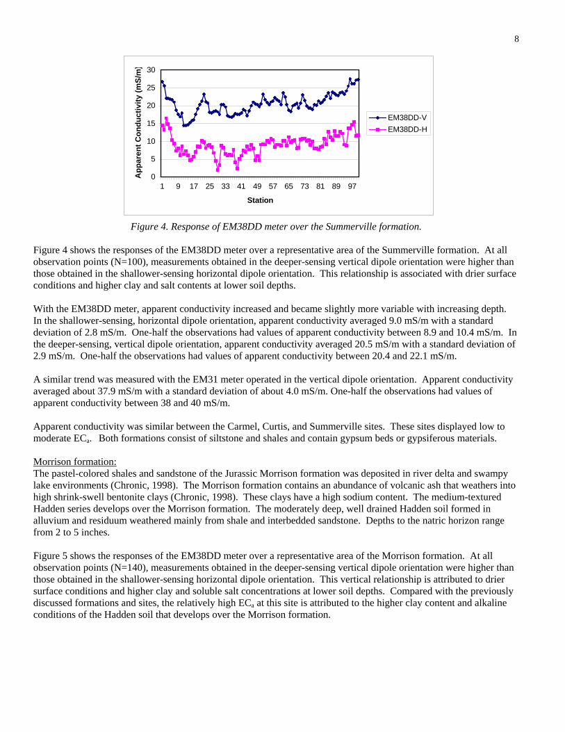
The increased conductivity with increasing depth was attributed principally to greater moisture, soluble salt, and clay contents at lower soil depths. Summerville Formation: The Jurassic Summerville formation forms gray and tan siltstone cliffs. The Summerville formation was originally deposited in tidal flats (Chronic, 1998). This formation contains an abundance of gypsum veins and is capped with a thick bed of gypsum deposited by the evaporation of salt water (Chronic, 1998). The Summerville formation is characterized by loamy Shalet series. The very shallow and shallow, well drained Shalet soil formed in residuum weathered from shale.
8
Figure 4. Response of EM38DD meter over the Summerville formation. Figure 4 shows the responses of the EM38DD meter over a representative area of the Summerville formation. At all observation points (N=100), measurements obtained in the deeper-sensing vertical dipole orientation were higher than those obtained in the shallower-sensing horizontal dipole orientation. This relationship is associated with drier surface conditions and higher clay and salt contents at lower soil depths. With the EM38DD meter, apparent conductivity increased and became slightly more variable with increasing depth. In the shallower-sensing, horizontal dipole orientation, apparent conductivity averaged 9.0 mS/m with a standard deviation of 2.8 mS/m. One-half the observations had values of apparent conductivity between 8.9 and 10.4 mS/m. In the deeper-sensing, vertical dipole orientation, apparent conductivity averaged 20.5 mS/m with a standard deviation of 2.9 mS/m. One-half the observations had values of apparent conductivity between 20.4 and 22.1 mS/m. A similar trend was measured with the EM31 meter operated in the vertical dipole orientation. Apparent conductivity averaged about 37.9 mS/m with a standard deviation of about 4.0 mS/m. One-half the observations had values of apparent conductivity between 38 and 40 mS/m. Apparent conductivity was similar between the Carmel, Curtis, and Summerville sites. These sites displayed low to moderate ECa. Both formations consist of siltstone and shales and contain gypsum beds or gypsiferous materials. Morrison formation: The pastel-colored shales and sandstone of the Jurassic Morrison formation was deposited in river delta and swampy lake environments (Chronic, 1998). The Morrison formation contains an abundance of volcanic ash that weathers into high shrink-swell bentonite clays (Chronic, 1998). These clays have a high sodium content. The medium-textured Hadden series develops over the Morrison formation. The moderately deep, well drained Hadden soil formed in alluvium and residuum weathered mainly from shale and interbedded sandstone. Depths to the natric horizon range from 2 to 5 inches. Figure 5 shows the responses of the EM38DD meter over a representative area of the Morrison formation. At all observation points (N=140), measurements obtained in the deeper-sensing vertical dipole orientation were higher than those obtained in the shallower-sensing horizontal dipole orientation. This vertical relationship is attributed to drier surface conditions and higher clay and soluble salt concentrations at lower soil depths. Compared with the previously discussed formations and sites, the relatively high ECa at this site is attributed to the higher clay content and alkaline conditions of the Hadden soil that develops over the Morrison formation.
0
5
10
15
20
25
30
1 9 17 25 33 41 49 57 65 73 81 89 97
Station
Ap
par
ent
Co
nd
uct
ivit
y (m
S/m
)
EM38DD-V
EM38DD-H

9
Figure 5. Response of EM38DD meter over the Morrison formation.
With the EM38DD meter, values of apparent conductivity were comparatively high and increased and became slightly more variable with increasing depth. In the shallower-sensing, horizontal dipole orientation, apparent conductivity averaged 14.4 mS/m with a standard deviation of 8.0 mS/m. One-half the observations had values of apparent conductivity between 12.8 and 19.0 mS/m. In the deeper-sensing, vertical dipole orientation, apparent conductivity averaged 37.2 mS/m with a standard deviation of 10.6 mS/m. One-half the observations had values of apparent conductivity between 35 and 45.1 mS/m. A similar trend was measured with the EM31 meter operated in the vertical dipole orientation. Apparent conductivity averaged 62.3 mS/m with a standard deviation of 12.9 mS/m. One-half the observations had values of apparent conductivity between 62 and 67.9 mS/m. Mancos formation: The Cretaceous Mancos formation consists principally of soft, fine, gray shales interspersed with thin coal beds (Chronic, 1998). This Mancos formation weathers into high shrink-swell clays and contains considerable amounts of salts. These salts are mostly calcium sulfate (gypsum), and calcium carbonate. The well drained, fine-textured Chipeta and Hanksville soils develop over the Mancos formation. The very shallow and shallow Chipeta and the moderately deep Hanksville soils formed in residuum, colluvium, and alluvium weathered from Mancos shale. These soils have relatively high calcium carbonate equivalent, sodium adsorption ratios, electrical conductivity, and gypsum contents. Figure 6 shows the responses of the EM38DD meter over a representative area of the Mancos formation. At all observation points (N=111), measurements obtained in the deeper-sensing vertical dipole orientation were higher than those obtained in the shallower-sensing horizontal dipole orientation. Compared with all sites, this site had the highest and most variable ECa. With the EM38DD meter, values of apparent conductivity were comparatively high and increased and became slightly more variable with increasing depth. In the shallower-sensing, horizontal dipole orientation, apparent conductivity averaged 23.2 mS/m with a standard deviation of 17.4 mS/m. One-half the observations had values of apparent conductivity between 16.0 and 23.9 mS/m. In the deeper-sensing, vertical dipole orientation, apparent conductivity averaged 49.0 mS/m with a standard deviation of 19.7 mS/m. One-half the observations had values of apparent conductivity between 40.5 and 55.2 mS/m.
0
10
20
30
40
50
60
1 20 39 58 77 96 115 134
Station
Ap
par
ent
Co
nd
uct
ivit
y (m
S/m
)
EM38DD-V
EM38DD-H

10
0
20
40
60
80
100
120
1 10 19 28 37 46 55 64 73 82 91 100 109
Station
Ap
par
ent
Co
nd
uct
ivit
y (m
S/m
)
EM38DD-V
EM38DD-H
Figure 6. Response of EM38DD meter over the Mancos formation.
A similar trend was measured with the EM31 meter operated in the vertical dipole orientation. Apparent conductivity averaged 67.7 mS/m with a standard deviation of 9.1 mS/m. One-half the observations had values of apparent conductivity between 64 and 71.5 mS/m. The higher relative ECa values are associated with higher clay and soluble salt contents of the Chipeta and Hanksville soils. The vertical relationship is associated with higher clay, moisture, and soluble salt concentrations at lower soil depths. Landscape Studies: Additional traverses were conducted with the EMI instruments in areas of the Carmel, Summerville, and Morrison formations. These traverses crossed several landscape components and contained a biased and disproportionately large number of measurements in dry washes. Salt flecks were observed on soil surfaces within the washes and these landscape components were known to contain higher levels of soluble salts. In general, apparent conductivity values increased and became more variable as the measurements from the washes were included in the data sets. For soils formed over the Carmel formation, the average conductivity increased from 19.7 and 10.2 mS/m to 32.4 and 24.9 mS/m in the vertical and horizontal dipole orientations, respectively. For soils formed over the Summerville formation, average conductivity increased from 20.5 and 9.0 mS/m to 28.9 and 15.7 mS/m in the vertical and horizontal dipole orientations, respectively. For soils formed over the Morrison formation, average conductivity increased from 37.2 and 14.4 mS/m to 62.6 and 37.2 mS/m in the vertical and horizontal dipole orientations, respectively. Over the Morrison formation, the maximum ECa measurements were recorded in both dipole orientations (139 mS/m in the vertical and 103 mS/m in the horizontal). These additional traverses were not used in the analysis of variance. Analysis of Variance: The analysis of variance was used to study whether the different formations contribute to the variability of apparent conductivity measurements. The null hypothesis was that the mean ECa for all formations (Carmel, Entrada, Curtis, Summerville, Morrison, and Mancos) is the same. As shown in Table 2, for measurements collected with the EM38DD meter in both dipole orientations, the mean ECa was significantly different among the six formations. Although the number of observations and sites were small, there appears to be highly significant differences in the average ECa among the formations. For ECa measurements collected in both dipole orientations, the Mancos and Morrison formations have the largest mean; the Entrada and Curtis formations have the lowest means. The results of this investigation suggest that EMI can be used to distinguish soils and geologic formations within the San Rafael River Basin.

11Table 2. Analysis of Variance of measured ECa over the six bedrock formations.
A. EM38DD-Vertical Dipole Orientation
Degree of Freedom Sum of Squares Mean Square F-value Probability Between 5 122600.706 24520.141 257.626 0.0000 Within 681 64815.669 95.177 Total 686 187416.375
Formation Observations Sum Average SD SE Carmel 94 1849.36 19.67 6.93 1.01 Entrada 127 1349.75 10.62 1.14 0.87 Summerville 100 2051.86 20.52 2.87 0.98 Curtis 115 1950.65 16.96 3.26 0.91 Morrison 140 5204.85 37.18 10.59 0.82 Mancos 111 5443.80 49.04 19.67 0.93 Total 687 17850.27 25.66 16.53 0.63 Within 9.76
B. EM38DD-Horizontal Dipole Orientation. Degree of Freedom Sum of Squares Mean Square F-value Probability Between 5 27964.391 5592.878 80.966 0.0000 Within 681 47041.207 69.077 Total 686 75005.598
Formation Observations Sum Average SD SE
Carmel 94 962.96 10.24 5.49 0.86 Entrada 127 426.26 3.36 1.62 0.74 Summerville 100 902.01 9.02 2.81 0.83 Curtis 115 787.72 6.85 2.64 0.78 Morrison 140 2017.60 14.41 7.97 0.70 Mancos 111 2574.64 23.20 17.45 0.79 Total 687 7671.19 11.18 10.46 0.40 Within 8.31
Grid Study Areas: Three sites adjoining the San Rafael River were selected for detailed EMI surveys. Each site contained soils that formed over different lithologies. Fuller Bottom: Two areas of alluvial and colluvial soils were surveyed within Fuller Bottom. Site is bounded on the east by the San Rafael River and on the south by bedrock escarpments (see eastern-most appendage in figures 7 and 8). Site 2, is higher lying and more distant to the San Rafael River than Site 1. The eastern portion of Site 2 contains several terraces of alluvial deposits and is bounded on the southeast by bedrock escarpments with narrow fans of colluvial deposits (see western, larger continuous area in figures 7 and 8). The western portion of Site 2 is higher lying and contains a large alluvial fan of coarse textured materials. Fuller Bottom is near the contact of the Jurassic age Entrada and Carmel formations. The Carmel is gypsiferous sandstone and shales with some soft gypsum bedrock. Entrada is sandstone.

12Table 3 summarizes EMI survey results from Site 1at Fuller Bottom. Within this site, apparent conductivity ranged from about 0.1 to 360 mS/m. With the EM38DD meter, apparent conductivity increased and became more variable with increasing depth. In the shallower-sensing, horizontal dipole orientation, apparent conductivity averaged 131.0 mS/m with a standard deviation of 73.1 mS/m. One-half the observations had values of apparent conductivity between 62.9 and 194.6 mS/m. In the deeper-sensing, vertical dipole orientation, apparent conductivity averaged 175.5 mS/m with a standard deviation of about 91.8 mS/m. One-half the observations had values of apparent conductivity between 94.5 and 257.2 mS/m. With the EM31 meter, apparent conductivity was only measured in the vertical dipole orientation. Apparent conductivity averaged 150.3 mS/m with a standard deviation of 68.3 mS/m. One-half the observations had values of apparent conductivity between 163.0 and 204.0 mS/m.
Table 3. Basic EMI Statistics for Site #1 Fuller Bottom. EM38DD-V EM38DD-H EM31-V Number 2084 2084 955 Minimum 11.5 0.02 25.0 Maximum 359.5 315.5 313.0 25%-TILE 94.5 62.9 163.0 75%-TILE 257.2 194.6 204.0 Average 175.5 131.0 150.3 Standard Deviation 91.8 73.1 68.3
Based on the responses of the EM38DD meter in the two dipole orientations, apparent conductivity generally increased with increasing soil depth across the site. However, comparing responses obtained with the EM38DD and EM31 meters in the vertical dipole orientation, apparent conductivity after peaking (as measured with the EM38DD meter) decreased with increasing soil depths (as measured with EM31 meter). In general, ECa in excess of 40 to 80 mS/m are indicative of high concentrations of soluble salts. Because of the prevalence of high apparent conductivity (values > 80 mS/m) measured at this site, the spatial and vertical (high values at intermediate depths) patterns are attributed principally to high concentrations of soluble salts. Table 4 summarizes EMI survey results from Site 2 at Fuller Bottom. Within this site, apparent conductivity ranged from about –26 to 293 mS/m. Negative values are attributed to calibration errors and were measured over higher lying, coarser textured alluvial fan that is located in the western and southwestern portions of the survey area. With the EM38DD meter, apparent conductivity increased and became more variable with increasing depth. In the shallower-sensing, horizontal dipole orientation, apparent conductivity averaged 14.4 mS/m with a standard deviation of 34.7 mS/m. One-half the observations had values of apparent conductivity between –8.6 and 26.0 mS/m. In the deeper-sensing, vertical dipole orientation, apparent conductivity averaged 51.4 mS/m with a standard deviation of 45.1 mS/m. One-half the observations had values of apparent conductivity between 19.5 and 69.4 mS/m.
Table 4. Basic EMI Statistics for Site #2 Fuller Bottom. EM38DD-V EM38DD-H EM31-V Number 2355 2355 4543 Minimum 0.25 -25.9 15.0 Maximum 259.4 189.8 293.0 25%-TILE 19.5 -8.6 77.0 75%-TILE 69.4 26.0 115.0 Average 51.4 14.4 87.6 Standard Deviation 45.1 34.7 50.8

13With the EM31 meter, apparent conductivity was only measured in the vertical dipole orientation. Apparent conductivity averaged 87.6 mS/m with a standard deviation of 50.8 mS/m. One-half the observations had values of apparent conductivity between 77.0 and 115.0 mS/m. In general, at Fuller Bottom, apparent conductivity increased laterally from exceedingly low values on the gravelly and coarser textured alluvial fan towards stream terraces composed of presumably finer-textured alluvial deposits from the San Rafael River. In addition, linear zones of high apparent conductivity bounded the short steep slopes of colluvium that fronted the bedrock escarpments in the southeast corner of the site. The colluvial deposits and the alluvial fans and cones are characterized by low apparent conductivity. Unlike Site 1 and with the exception of some alluvial deposits, there was no apparent peak of apparent conductivity at intermediate soil depths at Site 2. At Site 2 in Fuller Bottom, apparent conductivity increased with increasing soil depth. Figure 7 shows the spatial distribution of apparent conductivity across Fuller Bottom as measured with the EM38DD meter in the horizontal (upper map) and vertical (lower map) dipole orientations. Sites 1 and 2 have been complied together in these composite maps of Fuller Bottom. In each map, color variations have been used to show the distribution of apparent conductivity. In each map the isoline interval is 10 mS/m. The locations of observation points are shown in the upper map. The San Rafael River is shown in the extreme eastern portion of each map.
Horizontal Dipole Orientation
Vertical Dipole Orientation
4329100
4329200
4329300
4329400
Nor
thin
g
512600 512700 512800 512900 513000 513100 513200 513300 513400 513500
Easting
4329100
4329200
4329300
4329400
No
rth
ing
mS/m
-20020406080100120140160180200220240260280300320340360380400
San Rafael River
Observation Point
AB
AB
Figure 7. Maps of apparent conductivity obtained at the Fuller Bottom Site with the EM38DD meter.
Figure 8 shows the spatial distribution of apparent conductivity across Fuller Bottom as measured with the EM31 meter in vertical dipole orientations. In each map, color variations have been used to show the distribution of apparent conductivity. In each map the isoline interval is 10 mS/m. The locations of observation points and the San Rafael River are shown on this map. The areas surveyed with the EM38DD and EM31 meters were similar for the Site 2, but were slightly dissimilar for the Site 1 portions of the Fuller Bottom maps. Within Fuller Bottom, dense vegetation precluded the survey of areas to the northeast.

14
512600 512700 512800 512900 513000 513100 513200 513300 513400 513500
Easting
4329000
4329100
4329200
4329300
4329400
Nor
thin
g
San Rafael River
Observation Point
020406080100120140160180200220240260280300320340360380400
mS/m
AB
Figure 8. Apparent conductivity map of Fuller Bottom Site obtained with the EM31 meter in the vertical dipole
orientation. Apparent conductivity values in excess of 80 mS/m (yellow and red areas in figures 7 and 8) are presumed to reflect the concentration of soluble salts and the presence of saline soils. In figures 7 and 8, area with high apparent conductivity form coalescing linear bands on the flood plain of the San Rafael River in the eastern portion of the study area. In general, linear bands with the highest apparent conductivity appear to border bedrock escarpments, which form the southern boundary in the southeastern portions of these maps. These bands may represent relic channels of the San Rafael River. These bands appear to extend towards the San Rafael River. However, these linear features of higher apparent conductivity do not cross a lower-lying terrace (see A) composed of coarse-textured alluvial deposits that adjoins the river. An area of high apparent conductivity extends in an arc-like fashion across the western portion of the Fuller Bottom site. At deeper depths (see Figure 8), this arc is more continuous and appears to define the outer boundary of a coarse-textured alluvial fan (B) from which seepage or flow of salt contaminated groundwater is believed to have occurred. Entrada Unit: Table 5 summarizes the survey results from Entrada Site. Within this site, apparent conductivity ranged from about –7.5 to 264 mS/m. Negative values are attributed to calibration errors. With the EM38DD meter, apparent conductivity increased and became slightly more variable with increasing depth. In the shallower-sensing, horizontal dipole orientation, apparent conductivity averaged 21.4 mS/m with a standard deviation of 26.2 mS/m. One-half the observations had values of apparent conductivity between 6.0 and 30.9 mS/m. In the deeper-sensing, vertical dipole orientation, apparent conductivity averaged 32.4 mS/m with a standard deviation of 31.1 mS/m. One-half the observations had values of apparent conductivity between 13.8 and 44.5 mS/m. The increased conductivity with increasing depth is believed to be attributable to higher contents of soluble salts at greater soil depths.
Table 5. Basic EMI Statistics for Entrada Site. EM38DD-V EM38DD-H EM31-V Number 1977 1977 807 Minimum 1.9 -7.5 19.0 Maximum 263.6 200.9 147.2 25%-TILE 13.8 6.0 31.0 75%-TILE 44.5 30.9 45.2 Average 32.4 21.4 40.0 Standard Deviation 31.1 26.2 13.3

15With the EM31 meter, apparent conductivity was only measured in the vertical dipole orientation. Apparent conductivity averaged 40.0 mS/m with a standard deviation of 13.3 mS/m. One-half the observations had values of apparent conductivity between 31.0 and 45.2 mS/m. Figure 9 shows the spatial distribution of apparent conductivity across the Entrada Site as measured with the EM38DD meter in the horizontal (left-hand map) and vertical (right-hand map) dipole orientations. In each map, color variations have been used to show the distribution of apparent conductivity. In each map the isoline interval is 5 mS/m. The locations of the observation points are shown in the left-hand map. In each map, the location of the San Rafael River is labeled. Also shown in each map is the course of a small, deeply incised, dry wash that flows into the San Rafael River. Figure 10 shows the spatial distribution of apparent conductivity across the Entrada Site as measured with the EM31 meter in vertical dipole orientations. Color variations have been used to show the distribution of apparent conductivity. The isoline interval is 5 mS/m. The locations of the observation points are shown in the left-hand map. Operational and software problems prevented the recording of many EMI measurements with the EM31 meter. In addition, poorer resolution was obtained with this AG114 GPS receiver in this terrain. In Figure 10, the location of the San Rafael River is labeled. Immediately adjacent to the river, in a very narrow (3 ft wide) zone, inverted salt profiles were observed with the EM38DD meter. It is believed that water from the river is wicking upward in this zone and depositing salts on the surface. This was the only area surveyed with the EM38DD meter in the San Rafael Basin that had inverted salt profiles.
Horizontal Dipole Orientation Vertical Dipole Orientation
511200 511250 511300 511350 511400
EASTING
4330150
4330200
4330250
4330300
4330350
4330400
4330450
NO
RT
HIN
G
511200 511250 511300 511350 511400
EASTING
0102030405060708090100110120130140150160170180190200
San Rafael River
San Rafael River
Observation point
mS/m
A
B
A
B
Figure 9. Maps of apparent conductivity obtained at the Entrada Site with the EM38DD meter.
Alluvial deposits from the San Rafael River forms a rather narrow band across the southern portion of the survey area. In each of the maps in figures 9 and 10, a segmented brown line demarcates the boundary of the San Rafael River’s flood plain. In general, this band of alluvium has higher apparent conductivity than adjoining upland areas of presumably Moffat soils. In figures 9 and 10, areas of noticeably higher and anomalous apparent conductivity have

16been labeled A and B. At A, a zone of high apparent forms a distinct plume-like pattern that emanates from a bedrock escarpment, extends outwards, and dissipates towards the San Rafael River. The base of the escarpment is near the contact of the Entrada and Carmel formations, and the high apparent conductivity is attributed to soluble salts from the Carmel formation. At B, an incised dry wash cuts across exposed bedrock, this is also near the contact between the Entrada and Carmel formations.
511200 511250 511300 511350 511400
Easting
4330150
4330200
4330250
4330300
4330350
4330400
4330450
No
rthi
ng
0102030405060708090100110120130140150160170180190200
mS/m
Observation point
A
B
San Rafael River
Figure 10. Apparent conductivity of the Entrada Site obtained with the EM31 meter in the vertical dipole orientation.
Hambrick Bottom: Hambrick Bottom is composed of alluvial deposits from the Summerville and Morrison formations. Table 6 summarizes survey results from Hambrick Bottom Site. Within this site, apparent conductivity ranged from about –2 to 345 mS/m. Negative values are attributed to calibration errors. Once again, with the EM38DD meter, apparent conductivity increased and became slightly more variable with increasing depth. In the shallower-sensing, horizontal dipole orientation, apparent conductivity averaged 56.1 mS/m with a standard deviation of 61.0 mS/m. One-half the observations had values of apparent conductivity between about 9.9 and 79.8 mS/m. In the deeper-sensing, vertical dipole orientation, apparent conductivity averaged 84.4 mS/m with a standard deviation of 79.9 mS/m. One-half the observations had values of apparent conductivity between 22.1 and 121.5 mS/m. The increased conductivity with increasing depth is believed to be attributable principally to higher contents of soluble salts at greater soil depths. The high variability of EMI responses is attributed to variations in the concentration of soluble salts within this site.
Table 6. Basic EMI Statistics for Hambrick Bottom Site. EM38DD-V EM38DD-H EM31-V Number 3990 3990 2100 Minimum -2.4 -11.6 24.0 Maximum 345.2 265.6 277.5 25%-TILE 22.1 9.9 45.0 75%-TILE 121.5 79.8 129.0 Average 84.4 56.1 95.0 Standard Deviation 79.9 61.0 59.7

17 With the EM31 meter, apparent conductivity was only measured in the vertical dipole orientation. Apparent conductivity averaged 95.0 mS/m with a standard deviation of 59.7 mS/m. One-half the observations had values of apparent conductivity between 45.0 and 129.0 mS/m.
509500 509600 509700 509800
Easting
4331900
4332000
4332100
4332200
4332300
4332400
4332500
No
rth
ing
509500 509600 509700 509800
Easting
Horizontal Dipole Orientation Vertical Dipole Orientation
020406080100120140160180200220240260280300320340360380400
mS/m
San Rafael River
Observation Point
A
B
C
D
E
Figure 11. Maps of apparent conductivity obtained at the Entrada Site with the EM38DD meter.
509400 509450 509500 509550 509600 509650 509700 509750 509800 509850
Easting
4331950
4332000
4332050
4332100
4332150
4332200
4332250
4332300
4332350
4332400
4332450
4332500
4332550
Nor
thin
g
020406080100120140160180200220240260280300320340360380400
San Rafael River
Observation Point
mS/m
A
B
C
D
E
Figure 12. Apparent conductivity of the Hambrick Site obtained with the EM31 meter in the vertical dipole orientation.

18Figure 11 shows the spatial distribution of apparent conductivity across the Hambrick Site as measured with the EM38DD meter in the horizontal (left-hand map) and vertical (right-hand map) dipole orientations. In each map, color variations have been used to show the distribution of apparent conductivity. In each map the isoline interval is 10 mS/m. The locations of the observation points are shown in the left-hand map. In each map, a dark blue line (extreme southwest border of the study area) shows the location of the San Rafael River. The dark brown, segmented line shows the approximate location of a slight scarp or riser, which separates different terraces to the San Rafael River. Figure 12 shows the spatial distribution of apparent conductivity across the Hambrick Site as measured with the EM31 meter in vertical dipole orientations. Color variations have been used to show the distribution of apparent conductivity. In Figure 12, the isoline interval is 10 mS/m. The locations of the observation points recorded with the EM31 meter are shown in this map. Operational and software problems prevented the recording of some EMI measurements recorded with the EM31 meter. A dark blue line (extreme southwest border of the study area) shows the location of the San Rafael River. The dark brown, segmented line shows the approximate location of a slight scarp, which separates different terraces to the San Rafael River. High values of apparent conductivity (> 80 mS/m) are attributed to high concentrations of soluble salts. In figures 11 and 12, areas of high apparent conductivity form three conspicuous linear bands (see A, B and C in the right-hand maps of these figures) that border alluvial fans (see E) or cones, and bedrock escarpments (exposed bedrock extends along the entire eastern and northeastern borders of the Hambrick site). In general, these bands of high apparent conductivity appear to emanate from the bases of fans and escarpments and extend down slope towards the San Rafael River. Because of their orientation, it is doubtful that these bands represent relic channels of the San Rafael River. These bands of high apparent conductivity undoubtedly represent zones of subsurface seepage: areas that receive larger amounts of soluble salt and moisture. Comparing figures 11 and 12, it is apparent that conductivity peaks at intermediate depths (most pronounced responses appear to be recorded with the EM38DD meter in the vertical dipole orientation). However, at deeper depths (see response of EM31 meter, Figure 12), the conductive zones appear to be less intense, but laterally more extensive beneath the alluvial fans. These bands or seepage lines extend towards the San Rafael River. However, even the most extensive and conspicuous seepage zone (A in figures 11 and 12) does not appear to cross a lower-lying terrace (see segmented brown line) composed of presumably coarse-textured alluvial deposits that adjoin the San Rafael River. An arrow indicates the assumed direction of flow, which leads directly towards the river near D. In the maps of data collected with the two meters in the vertical dipole orientation, a weak zone of higher apparent conductivity appears to extend from D towards seepage line A. Greasewoods were the dominant plant over seepage line A. These plants are more tolerant of, and tend to cycle and collect salts. All seepage areas were generally covered with reddish soils eroded from the Summerville formation. However, within the Hambrick site, not all areas of reddish soils have higher conductivities. Also shown in Figure 11 are the locations of three piezometers. The maps of apparent conductivity for the three sites along the San Rafael River will hopefully aid investigators better understand the hydrogeology of these sites and locate additional sites for the installation of piezometers. Conclusions: At all three detailed survey sites, linear or plume-like features of high (>80 mS/m) apparent conductivity were observed. In general, ECa in excess of 40 to 80 mS/m are indicative of high concentrations of soluble salts. Generally, in these areas, the contribution of salts far outweighs the contribution of moisture, clay content, clay type, and cation exchange capacity on apparent conductivity. The location and orientation of these lines or plume-like features of higher ECa suggest seepage from adjoining fans and bedrock escarpments. Salt-bearing waters appear to drain from the base of some bedrock escarpments. These waters leave high concentrations of residual salts in the soil near the bases of fans and escarpments. While high concentrations of soluble salts occur in many of the geologic formations within the San Rafael River Basin, no upland site contained as high or as extensive an area of high apparent conductivity as the areas investigated along the floodplain of the San Rafael River.

19References: Chronic, H. 1998. Roadside Geology of Utah. Mountain Press Publishing Company, Missoula, Montana. Cook, P. G. and B. G. Williams. 1998. Electromagnetic Induction Techniques; Part 8 of the Basics of recharge and discharge. CSIRO Publishing, Collingwood, Australia. Corwin, D. L. and J. D. Rhoades. 1984, Measurements of inverted electrical conductivity profiles using electromagnetic induction. Soil Sci. Soc. Am. J. 48: 288-291. Corwin, D. L. and J. D. Rhoades. 1990. Establishing soil electrical conductivity – Depth relations from electromagnetic induction measurements. Commun. In Soil Sci. Plant Anal. 21(11&12): 861-901. de Jong, E., A. K. Ballantyne, D. R. Cameron, and D. L. Read. 1979. Measurement of apparent electrical conductivity of soils by an electromagnetic induction probe to aid salinity surveys. Soil Sci. Soc. Am. J. 43:810-812. Diaz, L., and J. Herrero. 1992. Salinity estimates in irrigated soils using electromagnetic induction. Soil Sci. 154(2): 151-157. Geonics Limited. 2000. EM38DD ground conductivity meter: Dual dipole version operating manual. Geonics Ltd., Mississauga, Ontario. Greenhouse, J. P., and D. D. Slaine. 1983. The use of reconnaissance electromagnetic methods to map contaminant migration. Ground Water Monitoring Review 3(2): 47-59. Hadley, H. 2002. Transit sources of salinity loading in the San Rafael River, Colorado River Basin, Utah. Executive Project Summary. USDI BLM, Salt Lake City, Utah. Kachanoski, R. G., E. G. Gregorich, and I. J. Van Wesenbeeck. 1988. Estimating spatial variations of soil water content using noncontacting electromagnetic inductive methods. Can. J. Soil Sci. 68:715-722. Law, J. P. Jr., and A. G. Hornsby. 1982. The Colorado River salinity problem: Water Supply and Management 6(1-2): 87-104. McNeill, J. D. 1980a. Electromagnetic terrain conductivity measurement at low induction numbers. Technical Note TN-6. Geonics Ltd., Mississauga, Ontario. McNeill, J. D. 1980b. Electrical Conductivity of soils and rocks. Technical Note TN-5. Geonics Ltd., Mississauga, Ontario. p. 22. Palacky, G. J. 1987. Clay mapping using electromagnetic methods. First Break 5(8): 295-306. Rhoades, J. D., P. A. Raats, and R. J. Prather. 1976. Effects of liquid-phase electrical conductivity, water content, and surface conductivity on bulk soil electrical conductivity. Soil Sci. Soc. Am. J. 40:651-655. Sinha, A. K., D. C. Gresham, and L. E. Stephens. 1985. Deep electromagnetic mapping of sedimentary formations in Southern Ontario. Current Research, Part B, Geol. Survey of Canada. Paper 85-1B: 199-204. van der Lelij, 1983. Use of electromagnetic induction instrument (Type EM-38) for mapping soil salinity. Water Resources Commission, Murrumbidgee Division, New South Wales, Australia. 14 p. Williams, B. G., and G. C. Baker. 1982. An electromagnetic induction technique for reconnaissance surveys of soil salinity hazards. Australian Journal of Soil Res. 20: 107-118.

20Zalasiewicz, J. A. S. J. Mathers, and J. D. Cornwell. 1985. The application of ground conductivity measurements to geological mapping. Q. J. Eng. Geol. London 18: 139-148. Wollenhaupt, N. C., J. L. Richardson, J. E. Foss, and E. C. Doll. 1986. A rapid method for estimating weighted soil salinity from apparent soil electrical conductivity measured with an aboveground electromagnetic induction meter. Can J. Soil Sci. 66:315-321