Embed Size (px)
Citation preview
Universidade de Lisboa
Faculdade de Ciências
Departamento de Engenharia Geográfica, Geofísica e Energia
The dynamics of convective orographic precipitation: the transition to
convection
Miguel Nogueira
Doutoramento em Ciências Geofísicas e da Geoinformação
(Meteorologia)
2014

Universidade de Lisboa
Faculdade de Ciências
Departamento de Engenharia Geográfica, Geofísica e Energia
The dynamics of convective orographic precipitation: the transition to
convection
Miguel Nogueira
Tese orientada por:
Professor Doutor Pedro M. A. Miranda
Professora Doutora Ana P. Barros
Tese especialmente elaborada para a obtenção do grau de Doutor em Ciências
Geofísicas e da Geoinformação (Meteorologia)
2014

i
Contents
Acknowledgements ..................................................................................................................... iv
Abstract ........................................................................................................................................ v
Resumo ........................................................................................................................................ vi
List of acronyms and abbreviations ............................................................................................. x
List of symbols ........................................................................................................................... xii
1 Introduction ................................................................................................................................ 1
2 Multifractal properties of embedded convective structures in orographic precipitation: toward
subgrid-scale predictability ........................................................................................................... 8
2.1 Introduction ............................................................................................................................. 9
2.2 Numerical simulations .......................................................................................................... 13
2.3 Dynamical interpretation: linear stability analysis ............................................................... 17
2.4 Empirical scaling analysis ...................................................................................................... 19
2.4.1 The Universal Multifractal model ....................................................................................... 19
2.4.2 Scaling in simulated 2D fields ............................................................................................ 21
2.4.3 Scaling in cloud simulated fields – 3D analysis ................................................................. 27
2.4.4. Relations between different scaling fields ......................................................................... 35
2.4.5 Spectral Analysis ................................................................................................................ 37
2.5 Summary and discussion ........................................................................................................ 40
ii
3 Transient Stochastic Downscaling of Quantitative Precipitation Estimates for Hydrological
Applications ................................................................................................................................. 45
3.1 Introduction ............................................................................................................................ 46
3.2 Data and Methodology ........................................................................................................... 50
3.2.1 Datasets ............................................................................................................................... 50
3.2.2 Scaling analysis ................................................................................................................... 52
3.3 Scaling behavior of rainfall fields .......................................................................................... 54
3.3.1 Ensemble scaling analysis ................................................................................................... 54
3.3.2 Cluster Analysis .................................................................................................................. 58
3.4 Fractal dimension of the rain support .................................................................................... 63
3.5 Spatial downscaling ............................................................................................................... 66
3.5.1 Error analysis ...................................................................................................................... 68
3.5.2 Hydrological Applications .................................................................................................. 71
3.6 Conclusions ............................................................................................................................ 74
4 The non-convective/convective structural transition in stochastic scaling of atmospheric fields
....................................................................................................................................................... 78
4.1 Introduction ............................................................................................................................ 79
4.2 Data and methodology ........................................................................................................... 85

iii
4.2.1 Numerical simulations ........................................................................................................ 85
4.2.2 Multifractal framework ....................................................................................................... 87
4.3 Central Andes simulation results ........................................................................................... 90
4.4 Statistical scaling analysis ...................................................................................................... 94
4.4.1 Ensemble scaling analysis ................................................................................................... 94
4.4.1.1 Kinetic energy spectral analysis ....................................................................................... 94
4.4.1.2 Atmospheric water spectral analysis ................................................................................ 97
4.4.1.3 Moment scaling analysis ................................................................................................ 99
4.4.2 Transient scaling analysis ................................................................................................ 102
4.4.2.1 Transient spectral analysis ............................................................................................. 102
4.4.2.2 Transient moment scaling analysis ............................................................................... 107
4.5 Sub-grid scale statistics of atmospheric moisture ................................................................ 109
4.6 Conclusions .......................................................................................................................... 113
5 Overall conclusions ................................................................................................................. 117
References .................................................................................................................................. 124
iv
Acknowledgements
I would like to thank both my advisors, Professor Pedro Miranda and Professor Ana Barros for
their scientific guidance, support and for providing me with the opportunity to work in two
fantastic research teams, both at Instituto Dom Luiz at the University of Lisbon and also at Duke
University. I want to acknowledge all my colleagues in both groups with whom I had the
pleasure of spending these past years. In particular I am grateful to Jing Tao for her tireless help
with the hydrological modeling experiments and to Xiaoming Sun for sharing his remarkable
WRF simulation efforts over the Andes.
I acknowledge the funding I received from the Fundação para a Ciência e Tecnologia (F.C.T.)
under doctoral grant SFRH/BD/61148/2009. I also acknowledge the funding I received from project
SMOG (Structure of MOist convection in high-resolution GNSS observations and models)
funded by the Portuguese Science Foundation (PTDC/CTE-ATM/119922/2010) and project
IPHEx (Integrated Precipitation and Hydrology Experiment) at Professor Barros research group at Duke
University during this final year of my PhD, supported by NASA grant NNX13AH39G.
Agradeço todo o apoio que recebi da minha mãe, pai, avó e irmão, à família Albergaria e aos
meus amigos. Finalmente agradeço à Raquel pelo apoio incondicional sem o qual não teria
possível chegar aqui e ao Francisco pela enorme alegria que nos trouxe ao longo destes últimos
meses.
v
Abstract
Multifractal behavior holds to a remarkable approximation over wide ranges of spatial scales in
orographic rainfall and cloud fields. The scaling exponents characterizing this behavior are
shown to be fundamentally transient with nonlinear dependencies on the particular atmospheric
state and terrain forcing. In particular, a robust transition is found in the scaling parameters
between non-convective (stable) and convective (unstable) regimes, with clear physical
correspondence to the transition from stratiform to organized convective orographic
precipitation. These results can explain two often reported scaling regimes for atmospheric wind,
temperature and water observations. On the one hand, spectral slopes around 2-2.3 arise under
non-convective or very weak convective conditions when the spatial patterns are dominated by
large-scale gradients and landform. On the other hand, under convective conditions the scaling
exponents generally fluctuate around 5/3, in agreement with the Kolmogorov turbulent regime
accounting for the intermittency correction.
High-resolution numerical weather prediction (NWP) models are able to reproduce the
ubiquitous scaling behavior of observed atmospheric fields down to their effective resolution
length-scale, below which the variability is misrepresented by the model. The effective
resolution is shown to be a transient property dependent on the particular simulated conditions
and NWP formulation, implying that a blunt decrease in grid spacing without adjusting
numerical techniques may not lead to the improvements desired.
Finally, the application of transient spatial scaling behavior for stochastic downscaling and sub-
grid scale parameterization of cloud and rainfall fields is investigated. The proposed fractal
methods are able to rapidly generate large ensembles of high-resolution statistically robust fields
from the coarse resolution information alone, which can provide significant improvements for
stochastic hydrological prediction and associated extreme event forecasting and risk
management, and also for stochastic sub-grid parameterization of clouds with large potential to
improve the current state-of-the-art cloud parameterization schemes.
KEYWORDS: orographic precipitation; convection; multifractals; stochastic parameterization;
downscaling.
vi
Resumo
A presente tese focou-se na dinâmica da precipitação orográfica, com particular interesse na
transição para o regime convectivo que pode ser responsável por eventos de precipitação
extrema, com riscos naturais importantes associados como inundações rápidas, deslizamentos de
terras e avalanches de sedimentos. Os eventos de precipitação convectiva representam um
enorme desafio do ponto de vista da previsão operacional devido ao seu carácter turbulento, com
estrutura localizada e altamente transiente. Os modelos lineares conseguem explicar algumas
propriedades importantes da iniciação de convecção e estrutura espacial dos campos resultantes
de precipitação e nuvens orográficas, no entanto não conseguem fazer qualquer previsão
quantitativa e só conseguem prever qualitativamente a estrutura (aproximadamente) correta em
casos muito particulares. Isto deve-se essencialmente ao facto da importância de inúmeras
interações não lineares na dinâmica destes eventos não poder ser ignorada. No presente estudo,
investigou-se a estrutura multifractal dos campos de nuvens e precipitação orográfica,
representando uma aproximação notável para as observações consideradas numa vasta gama de
escalas espaciais desde comprimentos da ordem de 1 km até valores superiores a 500 km, capaz
de representar a estrutura complexa destes campos com variabilidade numa vasta gama de
escalas, resultante da interação de diversos processos não lineares com forte influência
orográfica. Mostrou-se que o comportamento multifractal é deformando pela presença de
numerosos zeros, característicos em campos de nuvens e precipitação devido à presença de
limiares associados às transições de fase e outros efeitos não lineares. Utilizou-se análise de
clusters para isolar as regiões chuvosas (i.e. regiões conexas sem zeros) realizando a análise
multifractal apenas nestas regiões, recuperando a sua estrutura multifractal não deformada.
A análise multifractal de campos atmosféricos observados e simulados numericamente
mostraram que os expoentes fractais que caracterizam o comportamento estocástico de
invariância de escala são intrinsecamente transientes, com dependências não lineares nas
condições particulares do estado da atmosfera e de forçamento topográfico. Em particular,
encontraram-se ligações entre estes parâmetros e a velocidade média do vento, a forma do
terreno e a estabilidade estática da atmosfera. Um resultado particularmente robusto foi a
transição nos parâmetros fractais entre os regimes não-convectivo (estável) e convectivo
(instável), com clara correspondência física com a transição entre precipitação orográfica

vii
estratiforme e convectiva. Estes resultados mantêm-se válidos para análise espectral de Fourier,
escalamento dos momentos estatísticos e funções estruturais, mesmo quando a deformação do
comportamento multifractal devido à presença de zeros é explicitamente tomada em
consideração. Estes resultados explicam dois regimes de invariância de escala amplamente
encontrados em campos atmosféricos de vento, temperatura e água suas diversas fases. Por um
lado, exponentes espectrais com valores de 2-2.3 surgem em situações não-convectivas ou com
estruturas convectivas fracas, quando as distribuições espaciais são dominadas por gradientes de
larga escala ou pela topografia. De facto, as propriedades de invariância de escala nestas
situações são semelhantes ao comportamento fractal observado nos respetivos campos de
elevação topográfica. Por outro lado, em condições convectivas os expoentes espectrais flutuam
em torno do valor 5/3, de acordo com as previsões de Kolmogorov para o regime turbulento
tomando em consideração as correções associadas à intermitência. O parâmetro de intermitência
multifractal mostrou um comportamento semelhante, dando mais robustez aos resultados
obtidos. Adicionalmente a simetria horizontal pode ser quebrada em certas ocasiões, gerando
anisotropia horizontal no comportamento multifractal com importantes impactos nos campos
atmosféricos.
Os modelos numéricos de previsão meteorológica são capazes de reproduzir o comportamento
multifractal observado em campos atmosféricos até à escala correspondente à sua resolução
efetiva. Abaixo desta escala a variabilidade é representada de forma errónea pelos modelos.
Mostrou-se que a resolução efetiva é uma propriedade transiente que depende das condições
particulares do sistema simulado e da própria formulação do modelo numérico, com particular
sensibilidade a parametrização dos efeitos turbulentos de sub-escala e à difusão numérica,
geralmente introduzida para manter a estabilidade das soluções numéricas. Estes efeitos tendem
a causar uma remoção excessiva de variabilidade nas pequenas escalas, onde os expoentes
espectrais apresentam valores não físicos superiores a 3. Nas escalas superiores à resolução
efetiva o modelo representa de forma adequada a estrutura da atmosfera, mostrando que o
aumento de resolução dinâmico realizado pelos modelos numéricos a partir do forçamento de
resolução grosseira é capaz de conservar e representar as propriedades multifractais da
atmosfera. Em particular, os resultados mostraram que nos casos convectivos o aumento de
resolução de 6 km, onde um esquema de parametrização para a convecção tem que ser
introduzido, para uma resolução de 1.2 km, onde as estruturas convectivas são parcialmente
viii
resolvidas, resultou num aumento de resolução efetiva consideravelmente inferior à diminuição
do espaçamento da grelha. Este resultado implica que a diminuição do espaçamento da grelha
(i.e. aumento da resolução) por si só, sem um ajustar das técnicas de modelação numérica,
poderá não levar à melhoria dos resultados da simulação desejados.
Investigou-se o potencial do comportamento multifractal transiente para aplicações estocásticas
de parametrização de sub-escala e de aumento de resolução em campos de nuvens e precipitação.
Os métodos fractais propostos têm a habilidade de gerar de forma célere numerosas realizações
de alta-resolução estatisticamente robustas apenas a partir da informação de resolução grosseira,
preservando a estrutura do forçamento e adicionando informação estatística útil nas escalas não
resolvidos. No caso de aumento de resolução estocástico, a geração destes conjuntos de soluções
plausíveis, todas elas com a estrutura estocástica coerente, é capaz de suprimir a lacuna de
resolução entre os campos observados e simulados e as necessidades de alta resolução de muitas
aplicações hidrometeorlógicas. Os resultados mostram que a metodologia proposta permite
melhorias significativas na previsão probabilística de variáveis hidrometeorológicas, com
importantes consequências para a previsão de eventos extremos e gestão de risco. No caso da
parametrização estocástica de sub-escala de nuvens a distribuição de probabilidades é obtida com
base em argumentos fractais. Os resultados mostraram que estes métodos representam uma
melhoria considerável na representação da distribuição de probabilidades relativamente à
distribuição log-normal, tanto nos extremos da distribuição como para intensidades intermédias.
De facto, a parametrização estocástica fractal apresenta grande potencial para obter melhorias
relativamente aos esquemas de parametrização do atual estado da arte. Adicionalmente
consideração do comportamento transiente nestas metodologias fractais permite obter melhores
representações da estrutura estatísticas de sub-escala, providenciando mais um argumento em
favor do comportamento transiente da estrutura estatística da atmosfera. No entanto, a
determinação a priori dos parâmetros fractais a partir da informação de resolução grosseira
representa uma questão complexa e não resolvida, devido às numerosas dependências não-
lineares que os parâmetros fractais apresentam e à reduzida dimensão da amostra que geralmente
se verifica quando a análise estatística se baseia apenas numa realização dos campos de
resolução grosseira. No caso de geração de campos de precipitação de alta-resolução para
forçamento de modelos hidrológicos mostrou-se que a determinação transiente dos expoentes
espectrais a partir da informação de resolução grosseira representa uma boa aproximação, com

ix
resultados notavelmente superiores ao uso de outros métodos de interpolação não fractal, como
por exemplo métodos bilineares. No entanto, este tipo de metodologia só pode ser usado quando
os campos de resolução grosseira contêm informação suficiente que permitia uma análise
estatística robusta, o que nem sempre se verifica. No caso de parametrização de sub-escala de
nuvens, mostrou-se que o comportamento das caudas das distribuições de probabilidade são bem
representadas quando se consideram valores para o expoente fractal de aproximadamente 5/3 no
caso convectivo e aproximadamente 2.1 em casos não-convectivos ou se existirem apenas
estruturas convectivas fracas. Finalmente mostrou-se que este tipo de métodos estocásticas
baseados na estrutura fractal da atmosfera obtém melhores resultados quando usados para obter
distribuições estatísticas plausíveis das variáveis de sub-escala e as respetivas incertezas, e não
como métodos deterministas para gerar uma única realização de sub-escala, geralmente obtida
como a média de várias realizações plausíveis o que introduz efeitos de alisamento. Este
resultado está de acordo com a natureza estocástica dos métodos fractais e dos próprios sistemas
turbulentos.
PALAVRAS CHAVE: precipitação orográfica, convecção; multifractais, parametrização
estocástica; aumento de resolução

x
List of acronyms and abbreviations
CAPE Convective Available Potential Energy
CIN Convective INhibition
DTM Double Trace Moment
EFPRB East Fork Pigeon River Basin
ERA European center for medium-range weather forecast Re-Analysis
fBS Fractional Brownian Surface
GATE Global atmospheric research program Atlantic Tropical Experiment
GFS Global Forecast System
HRDI High Resolution Domain of Interest
IPHEx Integrated Precipitation and Hydrology Experiment
LST Local Solar Time
MCS Mesoscale Convective System
MPAS Model for Prediction Across Scales
NCEP National Center for Environmental Prediction
NCEP/CPC National Center for Environmental Prediction Climate Prediction Center
NEXRAD Next generation Radar Network
NMQ National Mosaic and multisensor Quantitative precipitation estimates
NOAA National Oceanic and Atmospheric Administration
NSSL National Severe Storms Laboratory
NWP Numerical Weather Prediction
PDF Probability Distribution Function
PRB Pigeon River Basin
QPE Quantitative Precipitation Estimates

xi
SALLJ South Americal Low Level Jet
TRMM Tropical Rainfall Measuring Mission
UM Universal Multifractal
WFPRB West Fork Pigeon River Basin
WRF Weather Research and Forecast
xii
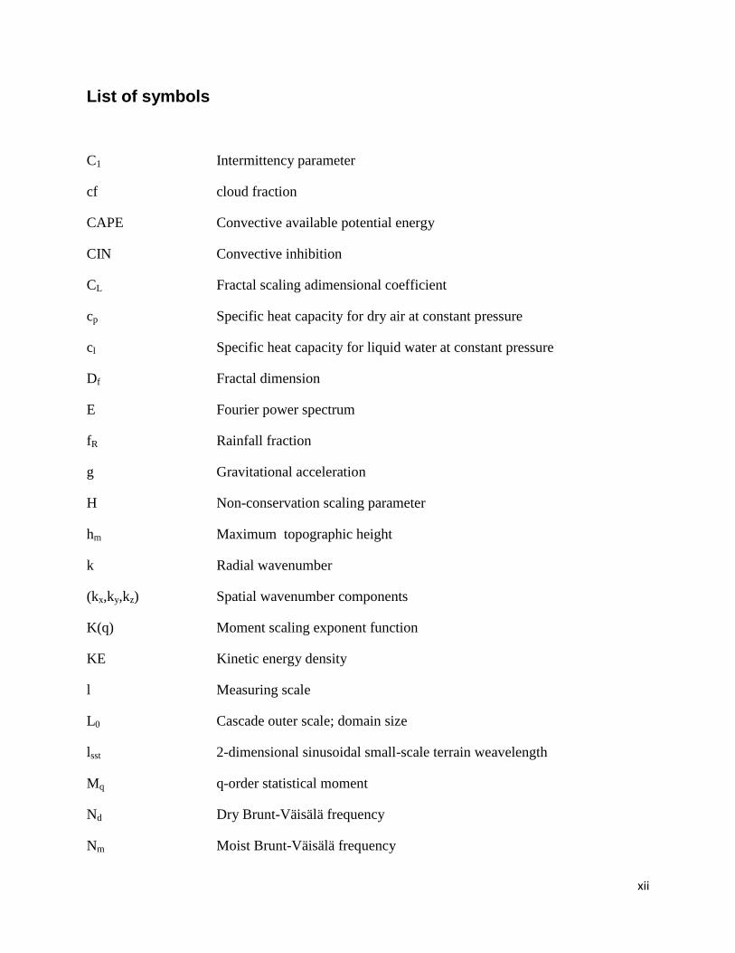
List of symbols
C1 Intermittency parameter
cf cloud fraction
CAPE Convective available potential energy
CIN Convective inhibition
CL Fractal scaling adimensional coefficient
cp Specific heat capacity for dry air at constant pressure
cl Specific heat capacity for liquid water at constant pressure
Df Fractal dimension
E Fourier power spectrum
fR Rainfall fraction
g Gravitational acceleration
H Non-conservation scaling parameter
hm Maximum topographic height
k Radial wavenumber
(kx,ky,kz) Spatial wavenumber components
K(q) Moment scaling exponent function
KE Kinetic energy density
l Measuring scale
L0 Cascade outer scale; domain size
lsst 2-dimensional sinusoidal small-scale terrain weavelength
Mq q-order statistical moment
Nd Dry Brunt-Väisälä frequency
Nm Moist Brunt-Väisälä frequency
xiii
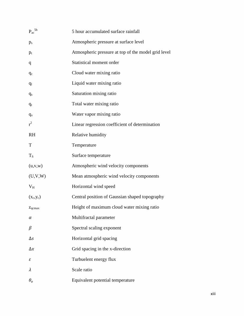
Pac5h
5 hour accumulated surface rainfall
ps Atmospheric pressure at surface level
pt Atmospheric pressure at top of the model grid level
q Statistical moment order
qc Cloud water mixing ratio
ql Liquid water mixing ratio
qs Saturation mixing ratio
qt Total water mixing ratio
qv Water vapor mixing ratio
r2 Linear regression coefficient of determination
RH Relative humidity
T Temperature
TS Surface temperature
(u,v,w) Atmospheric wind velocity components
(U,V,W) Mean atmospheric wind velocity components
VH Horizontal wind speed
(xc,yc) Central position of Gaussian shaped topography
zqcmax Height of maximum cloud water mixing ratio
Multifractal parameter
Spectral scaling exponent
Horizontal grid spacing
Grid spacing in the x-direction
Turbuelent energy flux
Scale ratio
Equivalent potential temperature
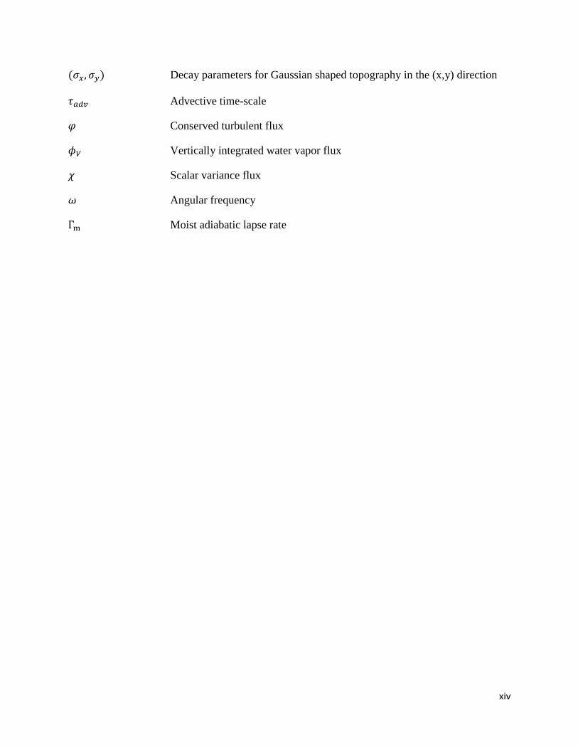
xiv
Decay parameters for Gaussian shaped topography in the (x,y) direction
Advective time-scale
Conserved turbulent flux
Vertically integrated water vapor flux
Scalar variance flux
Angular frequency
Moist adiabatic lapse rate
1
1 Introduction
Orography plays a fundamental role in the interaction between the land surface and the
atmosphere on a wide variety of spatial and temporal scales, one of its most important effects
being the modulation of rainfall patterns. The persistent topographic forcing is a major control on
the global precipitation, widespread to all climate zones, commonly dominating the
hydroclimatology over mountainous regions, causing differences in the mean annual
precipitation of several hundred percent between windward slopes of orographic barriers and
adjacent valleys or lee side slopes, giving rise to some of the most intense rainfall gradients on
Earth and playing a major role in extreme precipitation events (e.g. Barros and Lettenmaier,
1994; Lang and Barros, 2002; Barros and Lang, 2003; Garreaud et al., 2003; Barros et al., 2004,
2006; Roe, 2005; Smith, 2006; Zipser et al., 2006; Bhusan and Barros, 2007; Giovanettone and
Barros, 2009; Romatschke and Houze, 2010; Rasmussen and Houze Jr., 2011; Houze, 2012).
Consequently, orographic precipitation processes have profound impacts far beyond the field of
meteorology, affecting natural ecosystems, hydrology, agriculture, water resources and natural
hazards management, and even the geology of many regions.
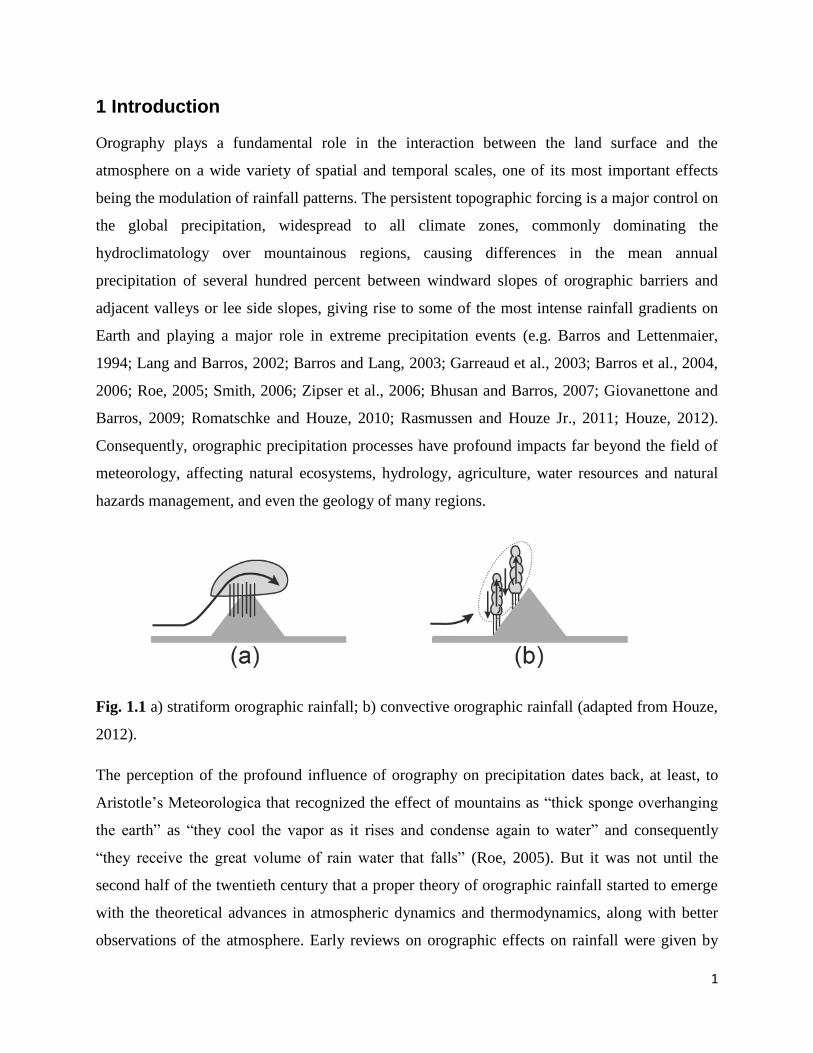
Fig. 1.1 a) stratiform orographic rainfall; b) convective orographic rainfall (adapted from Houze,
2012).
The perception of the profound influence of orography on precipitation dates back, at least, to
Aristotle’s Meteorologica that recognized the effect of mountains as “thick sponge overhanging
the earth” as “they cool the vapor as it rises and condense again to water” and consequently
“they receive the great volume of rain water that falls” (Roe, 2005). But it was not until the
second half of the twentieth century that a proper theory of orographic rainfall started to emerge
with the theoretical advances in atmospheric dynamics and thermodynamics, along with better
observations of the atmosphere. Early reviews on orographic effects on rainfall were given by
2
Queney et al. (1960) and Smith (1979). Fig. 1a shows the classical picture of orographic
precipitation where a prevailing wind is mechanically lifted over the windward flank, with moist
air ascending adiabatically above its saturation (cloud base) level and hence causing
condensation which leads to the generation and/or enhancement of clouds and precipitation. On
the leeward flank, the cloud is evaporated as the air becomes unsaturated due to the descending
motion together with decreased moisture and increased temperature caused by the windward
precipitation effects, resulting in the well-known rain shadow effect. Under unstable or
conditionally unstable conditions, the orographic uplift of the incoming flow together with
terrain induced perturbations can bring air parcels above their level of free convection, leading to
convective triggering and/or enhancement (Fig. 1b), strongly influencing the observed rainfall
amounts and distribution. In a seminal work, Kuo (1963) undertook an analytical analysis of a
linearized version of the Navier-Stokes equations to investigate convective triggering in unstable
fluid flow. This hypothesis has motivated the application of linear stability analyses to study
orographic convective precipitation, providing insight on the triggering, growth and structure of
convective features and highlighting the important role of small-amplitude topographic
variations in triggering and organizing orographic convection (Kirshbaum and Durran 2004,
2005a,b; Fuhrer and Schär, 2005, 2007; Kirshbaum et al., 2007a,b). Following these previous
investigations, the linearized Navier-Stokes, continuity and thermodynamic equations can be
reduced to a single wave equation for the vertical velocity, w, under the Boussinesq and inviscid
approximations and neglecting earth rotation:
(1.1)
Where U is the mean wind, and are respectively the three-dimensional and horizontal
Laplacian operator and is the moist Brunt-Väisälä frequency of the saturated layer given by
Eq. (1.2), which provides an appropriate measure of atmospheric stability in saturated layers as
discussed by Emanuel (1994).
(1.2)
Here ql represents the liquid water mixing ratio, is the moist adiabatic lapse rate, g is the
acceleration due to gravity, is the equivalent potential temperature and cp and cl are
3
respectively the specific heat capacity for dry air and liquid water at constant pressure. A
constant value is taken for in the linear framework for simplicity. By assuming plane-wave
perturbations as solutions to Eq. (1.1) given by and
considering solid wall boundary conditions at bottom and top boundaries, the following
dispersion relation can be extracted:
(1.3)
Where kx, ky and kz represent the spatial wavenumber components. In the case of statically
unstable stratification ( ) the physical solutions of the angular frequency, , equation are
exponentially growing waves advected by the flow (e.g. Fuhrer and Schar, 2005). The respective
growth rate for each small-scale disturbance mode of wavenumber can be
estimated as the imaginary part of . In this inviscid formulation, maximum growth is obtained
for largest possible vertical wavelength (limited by unstable cloud depth) and infinitesimally
small horizontal wavelength. Admitting that small-scale disturbances are ubiquitous in the real
atmosphere, this result was at odds the spatial scales and spacing between convective structures
observed in nature. More realistic solutions capable of representing the observed finite scales
governing orographic convective structures can be obtained by the introduction of a simplified
(linear) viscosity term that modulates the solutions, strongly increasing the growth times at small
horizontal wavelengths (Furher and Schar, 2005, 2007). Additionally, it has also been shown
that it is important to take into account the finite amplitude of topographic perturbations
upstream of the unstable cloud (Kirshbaum and Durran, 2007b) and to consider limited time-
scales for advection (i.e. the in-cloud residence time of air parcels, controlled by mean wind
speed and mountain width) and microphysical processes (i.e. the time period for rain production
and fallout) (Kirshbaum and Durran, 2004, 2007b). The linear stability analysis revealed some
ability in predicting the finite spacing between observed convective banded structures and their
initial growth rates for events over low elevation topography, but their main contribution is the
understanding of convective orographic features as the result of exponential growth of existing
small-scale atmospheric perturbations in an unstable stratified layer, pointing out the importance
of landform in controlling the location and occurrence of convective features, generating
4
unstable cap clouds by forced uplift of conditionally unstable flow and introducing finite
amplitude wave perturbations upstream of the orographic cloud.
Detailed observational and modeling studies have shown that orographic precipitation processes
encompass a rich set of physical processes such as forced uplift, blocking, channeling and
convergence effects, radiative effects of diurnal cycle and differential heating and the resulting
mesoscale breeze circulations, microphysical processes, seeder-feeder mechanisms, topographic
gravity waves and convective triggering (see e.g. Barros and Lettenmaier, 1994; Roe, 2005;
Smith, 2006 for reviews). Additionally, it was found that precipitation over and near mountains
is mostly caused by modulation of impinging synoptic-scale weather systems, particularly with
frontal systems, tropical cyclones and convective clouds (see Houze, 2012 for a recent review).
These numerous non-linear processes modulate the atmospheric fields over a vast span of spatial
and temporal scales, giving rise to complex orographic clouds and rainfall structures with
variability over a wide spectrum of scales, from synoptic to local and down to microphysics and
viscous dissipation scales. Investigations on the variability of orographic precipitation fields over
wide ranges of scales have revealed the presence statistical scale-invariant behavior (Harris et al.,
2001; Barros et al., 2004, 2006; Nykanen, 2008), hereafter referred to as scaling or fractal
behavior as commonly denoted in the atmospheric science literature. The idea of scaling
behavior derived from turbulent cascade schemes used to describe turbulent phenomenology
since Richardson (1922) and is theoretically supported by the scale invariance symmetries of the
Navier-Stokes equations governing atmospheric motion (Frisch, 1991). Over the past 30 years
numerous investigations have provided with vast evidence for the presence of scaling behavior in
atmospheric and other geophysical fields (see e.g. Veneziano et al., 2006; Lovejoy and Schertzer,
2007; Tuck, 2010 for reviews), implying that their statistical properties measured different scales
are related to each other by a scale-changing operation (generally a power law) that involves
only the scale ratio and a scaling exponent. Furthermore, these investigations have shown that for
geophysical fields the scaling is generally determined not by one, but by infinity scaling
exponents given by the scaling exponent function, i.e. they are multifractal. Complete
descriptions of the mathematical formulation and analysis tools of multifractal behavior together
with literature reviews on multifractal behavior in the atmosphere are provided is Chapters 2, 3
and 4 of the present thesis.
5
Numerical weather prediction (NWP) models represent a major research tool to investigate
precipitating-producing mechanisms given their encouraging performance to reproduce and
predict the main observed rainfall features (see e.g. Chow et al., 2013 for a recent discussion).
However, the large number of involved nonlinear processes occurring at vast ranges of spatio-
temporal scales drastically handicaps the ability of NWP models to provide with accurate
quantitative predictions of precipitation and clouds (Randall et al., 2013; Macilwain, 2014). In
particular, several deficiencies have been identified in terms of initiation, timing, intensity,
location and structure of simulated convective features (Kain et al., 2013). Despite the
considerable advances in computational power over the past decades, the allowed resolutions in
NWP forecasts (typically around 1 km) can only partially represent individual convective
elements and are altogether unable explicitly resolve very small-scale processes such as
turbulence and cloud microphysics, which can have large impacts on the dynamical evolution of
the atmosphere. Such fine resolutions as those required for resolving these effects will not be
attained for operational weather forecasts, at least over the next 10-20 years. In fact, physical
barriers might cause considerable issues in achieving such resolutions, for example power
consumption and hardware-related reliability of massively parallel computation (Wedi, 2014;
Macilwain, 2014). Consequently, the development of sub-grid parameterization strategies to
represent the effect of the unresolved scales on the solution represents a very active research
topic, posing a challenging problem because coarse and fine-scale fields are not mutually
dependent, since the knowledge of the resolved field does not imply the knowledge of the sub-
grid scale information, although the reverse is true. Despite the intensive efforts, the current sub-
grid representations are oversimplified and often nonphysical representations based on bulk
empirical formulas, with important impacts on the obtained solutions (e.g. Gianotti and Eltahir,
2013; Randall et al., 2013; Erlingis and Barros, 2014; Sun and Barros, 2014). Convective
orographic precipitation events are particularly problematic due to their sensitivity to
perturbations spanning over a wide range of scales introduced directly and indirectly (e.g. by
radiation processes) by numerous physical mechanisms associated with interactions between
atmosphere and terrain. In this sense, there is an urgent need to understand not only the physical
mechanisms involved, but also the relationships between atmospheric variables at different
spatial and temporal scales in order to obtain more realistic sub-grid scale parameterizations and
downscaling schemes, capable of bridging the gap in resolution between the typically available

6
observed and simulated rainfall fields and the high-resolution requirements of many
hydrometeorological applications, including water management and forecast of mountain
hazards such and flashfloods, landslides and debris flows (e.g. Barros and Lettenmaier, 1994;
Bindlish and Barros, 2000; Harris et al., 2001; Rebora et al., 2006, Tao and Barros, 2013,
2014a).
The present investigation aimed to improve the current limited understanding of orographic
rainfall processes, particularly the transition between stratiform and convective regimes,
traditionally used to classify orographic precipitation processes depending on the static stability
of the air masses impinging upon the topographic obstacle (Cotton and Anthes, 1989). The
presence of convective features can change the precipitation pattern and amount considerably,
and can lead to localized extreme values of rainfall responsible for mountain hazards including
landslides, debris flows and flashfloods. Additionally, three fundamental questions that currently
present a great challenge for modelers and forecasters are addressed:
i) how can the structure of different orographic precipitation events be characterized
based on the available knowledge of the dynamical atmospheric states?
ii) how is the transition between convective and stratiform regimes represented in such
characterization, and what is the respective impact of these regimes on the structures
of different atmospheric fields?
iii) how can this knowledge be used to improve the predictability of extreme events
associated with orographic convective rainfall and also for applications of
downscaling and sub-grid parameterization of rainfall and clouds fields?
This investigation was based on observations and high-resolution numerical simulations, both
under idealized and real case setups in which linear stability analysis and, particularly,
multifractal analysis are undertaken. Statistical multifractal analysis represents an important tool
to understand the relationships between the statistics of orographic precipitation fields at
different scales, with obvious importance and potential for sub-grid parameterization and
downscaling applications. While the scaling behavior does in fact seem to be a ubiquitous
property of atmospheric and geographical fields, the properties of such scaling behavior are
poorly understood. Notoriously, whether scaling parameters characterizing the multifractal
behavior of a given atmospheric field are universal (constant) as predicted by the classical

7
turbulence theory, or instead a transient property, is an important scientific question that remains
open. Furthermore, if the transient hypothesis is assumed, then the dynamical dependencies of
the scaling parameters must be investigated. Both these questions are thoroughly addressed in
Chapters 2, 3 and 4 of the present thesis. Particular emphasis is given to the investigation of the
possible differences between the statistical structure of stratiform and convective orographic
events.
This thesis is organized into five main chapters, where Chapters 2, 3 and 4 are presented as self-
contained scientific papers, published or submitted to publication. Chapter 5 summarizes the
main overall conclusions of this investigation and gives an outlook to future research topics.
In Chapter 2 a linear stability analysis was used to gain insight on triggering, growth and
structure of orographic rainfall and cloud fields generated by a population of three-dimensional
fully nonlinear idealized cloud resolving numerical simulations under different climatological
setups. The limitations of such simplified linearized theories and the extent to which they can be
used to fully understand, predict and quantify nonlinear orographic convective circulations is
investigated. The spatial scaling behavior of the simulated fields was also investigated, under a
transient multifractal framework. The linkages between the scaling parameters and the particular
atmospheric and terrain forcing were investigated, focusing on the transitions between stratiform
and convective regimes.
In Chapter 3 advantage was taken of high spatial and temporal resolution rainfall estimates based
on the dense weather radar network over the southern Appalachians. The effect of large zero
fractions in heavily thresholded rainfall fields on the spatial scaling behavior was investigated
and cluster analysis was used to characterize the scaling behavior of rainfall structures. Fractal
methods were used for downscaling applications taking explicitly into account the transient
nature of the scaling behavior. The resulting high-resolution rainfall products were tested as
forcing for hydrological models to obtain ensemble stochastic forecasts of streamflow.
Chapter 4 presents a case study of fully realistic high-resolution numerical simulations of deep
convective events under rainy season conditions and also dry winter conditions over the central
Andes region. The spatial scaling behavior of wind and atmospheric water content fields were
investigated, with particular focus on the non-convective/convective transition. Additionally, the
8
NWP effective resolution and sub-grid parameterization issues were investigated based on the
spectral scaling behavior. Finally, the application of transient scale-invariant behavior for
stochastic sub-grid parameterization of clouds is investigated.
9
2 Multifractal properties of embedded convective structures in
orographic precipitation: toward subgrid-scale predictability*
Abstract
Rain and cloud fields produced by fully nonlinear idealized cloud resolving numerical
simulations of orographic convective precipitation display statistical multiscaling behavior,
implying that multifractal diagnostics should provide a physically robust basis for the
downscaling and sub-grid scale parameterizations of moist processes. Our results show that the
horizontal scaling exponent function (and respective multiscaling parameters) of the simulated
rainfall and cloud fields varies with atmospheric and terrain properties, particularly small-scale
terrain spectra, atmospheric stability, and advective timescale. This implies that multifractal
diagnostics of moist processes for these simulations are fundamentally transient, exhibiting
complex nonlinear behavior depending on atmospheric conditions and terrain forcing at each
location. A particularly robust behavior found here is the transition of the multifractal parameters
between stable and unstable cases, which has a clear physical correspondence to the transition
from stratiform to organized (banded and cellular) convective regime. This result is reinforced by
a similar behavior in the horizontal spectral exponent. Finally, our results indicate that although
nonlinearly coupled fields (such as rain and clouds) have different scaling exponent functions,
there are robust relationships with physical underpinnings between the scaling parameters that
can be explored for hybrid dynamical-statistical downscaling.
* Nogueira
(1,2), M., Barros
(2), A. P., and Miranda
(1), P. M., 2013: Multifractal properties of
embedded convective structures in orographic precipitation: toward subgrid-scale predictability.
Nonlinear Processes in Geophysics, 20 (5), 605-620.
(1) CGUL-IDL, University of Lisbon, Portugal.
(2) Duke University, Durham, North Carolina, U.S.A.

10
2.1 Introduction
It is often observed that air masses impinging upon a mountain range lead to the development of
an orographic cloud with shallow embedded convective structures, which change the rainfall
pattern and amount considerably, and can lead to localized extreme values of rainfall. These
localized extremes present a great challenge for forecasters and are responsible for mountain
hazards including landslides, debris flows and flashfloods.
The notion that embedded convective structures are the result of exponential growth of small-
scale disturbances in an unstable stratified layer (Kuo, 1963) motivated the application of linear
stability analyses to gain insight on the dynamics of orographic convective precipitation,
including the estimation of the unstable growth rate, , for each small-scale disturbance mode of
wavenumber (Fuhrer and Schär, 2005):
(2.1)
(2.2)
where is the moist Brunt-Väisälä frequency of the saturated layer (as defined by Emanuel,
1994), which has a negative value in the moist unstable case. In this inviscid formulation, the
linear model predicts maximum growth for infinitesimally small horizontal wavelengths.
Admitting that small-scale disturbances are ubiquitous in the real atmosphere, this does not agree
with the observed finite spacing between bands observed in nature, for example: in western
Kyushu in Japan (Yoshizaki et al., 2000), in the Cévennes region in southern France (Miniscloux
et al., 2001; Cosma et al., 2002) and the Oregon Coastal Range (Kirshbaum and Durran, 2005b;
Kirshbaum et al., 2007b). Kirshbaum et al. (2007a) developed a new (also inviscid) linear model
that includes an upstream stable region where stationary small-scale lee waves are triggered and
subsequently used as the initial disturbances for the convective region. Their model agrees with
the results from numerical simulations that showed that such lee waves play a dominant role in
triggering and organizing banded convection with finite spacing (Kirshbaum and Durran, 2005a;
Fuhrer and Schär, 2007). Using both linear stability analysis and idealized numerical
simulations, additional factors were also found to be important such as: (i) cloud depth (which
11
determines the minimum value of allowed in Eq. 2.1) (Kirshbaum and Durran, 2004); (ii) the
advective timescale, i.e. the in-cloud residence time of air parcels which can be controlled by
mean wind speed and mountain width (Furher and Schär, 2005); (iii) dry stability outside the
cloud layer (Kirshbaum and Durran 2005a); and (iv) cloud base height (Kirshbaum et al., 2007a).
A different approach to the problem has gradually developed concurrent but separately in the last
thirty years, where the (statistical) scaling behavior of physical processes is explored. In these
processes the statistical properties of a field at different scales are related by a scale-changing
operation (generally a power law) that involves only the scale ratio and a scaling exponent, the
simplicity of which is very appealing for statistical downscaling applications. In geophysical
fields it is usually found that that the scaling is determined not by one, but by infinity of scaling
exponents given by the scaling exponent function, i.e. they are multiscaling. Schertzer and
Lovejoy (1987) proposed a functional form for this function, the Universal Multifractal (UM)
model, briefly presented in Section 2.4. There are a number of publications reporting
multiscaling behavior in various geophysical fields, including cloud and rain fields, over various
temporal (see e.g. de Lima and de Lima, 2008 for a review) and spatial ranges, e.g. Schertzer and
Lovejoy (1987). Nykanen (2008) found scaling on horizontal maps of radar rain reflectivity;
Gupta and Waymire (1990) found scaling on spatial fields of oceanic rainfall; Tessier et al.
(1993) and Barros et al. (2004) found scaling in satellite-based fields of cloud radiances.
Recently, Lovejoy et al. (2008a) looked at TRMM product 2A25 near surface reflectivity from
rain measurements and found evidence of multiplicative cascades from planetary scales down to
a few kilometers (~4 km, the data set resolution) in the ensemble averaged scaling statistics.
Also, note that the 2A25 product is an orbit based product with limited dimensions in the
direction perpendicular to eh satellite movement. They argued that the UM model with well
posed fixed values of the scaling parameters is a good approach when considering the entire
range of scales. Stolle et al. (2009) showed that data from global models (including ERA40
reanalysis and NOAA GFS) also accurately follow cascade statistics from nearly 20,000 km
down to around 100 km, where there was a cut off by hyper viscosity of the numerical model
linked to grid resolution.
However, there is no consensus on the specific values of the scaling exponents (and associated
UM parameters) and scaling ranges in the literature, although some of the differences might be
12
attributed to sample size or differences in measurements (sensors, measurement methods or
measurement errors, etc.). Another view is that the scaling exponents vary depending on
contextual environmental conditions, and therefore the observed variations can be attributed in
part o physical processes. Over and Gupta (1994) also used 2-dimensional oceanic rainfall fields
from GATE (GARP Atlantic Tropical Experiment), and proposed a relation between a scaling
parameter and large-scale average rain (argued to be an index of synoptic-scale weather
conditions); Perica and Foufoula-Georgiou (1996) related scaling parameters computed from
horizontal rainfall radar fields to the Convective Available Potential Energy (CAPE) of the pre-
storm environment over the same area; Deidda (2000) and Deidda et al. (2004) also found a
dependency in one of their scaling parameters computed from radar reflectivity on the large-
scale mean rainfall rate; and more recently Nykanen (2008) linked the variation in the values of
the multiscale statistical parameters computed from radar rainfall fields to the underlying
topographic elevation, predominant orographic forcing and storm location, and movement
relative to the orographic cross-sections. These results suggest that UM parameters vary from
event to event, or case-study to case-study as a function of atmospheric conditions, and local
terrain parameters. If this behavior can be translated into robust relationships between UM
parameters of particular states (e.g. precipitation) and the specific physical processes that
determine the space-time evolution of these states (e.g. moist convection), then inference and
induction modeling approaches can be used to develop quantitative dynamical models of the
state of interest relying on knowledge of the specific physical processes alone. For instance, to
predict precipitation fields over a wide range of spatial scales knowing atmospheric stability
conditions and precipitation at one (coarser) scale. This type of modeling could be used to
formulate parameterizations of unresolved processes in numerical weather and climate prediction
models, and to predict states at spatial resolutions much finer than those resolved by models, or
observations; that is, downscaling. In practical terms, this requires investigating possible
relationships between physical properties and statistical parameters that would allow statistical
downscaling from coarse to fine resolutions.
In the present work scaling analysis is performed on the output of highly idealized numerical
simulations, in particular on surface accumulated rainfall fields and horizontal cross section of
cloud water mixing ratio at several vertical levels. This gives us the opportunity to investigate
horizontal scaling at several vertical levels at the same time instant, obtaining a horizontal
13
scaling regime for 3-dimensional physically consistent fields, instead of 2-dimensional fields
used previously in the literature (see above). The behavior of the scaling parameters for varying
configurations of small-scale terrain and upstream profiles is investigated under different
idealized climatological regimes (presented in section 2.2), aiming to find physically based
relationships between scaling parameters and atmospheric and terrain properties that can be
estimated systematically from coarser resolution simulations. The paper is organized as follows:
Section 2.2 presents the numerical setup; a summary interpretation of the simulation results in
light of the linear theories is presented in Section 2.3; and the empirical scaling analysis is
presented in Section 2.4. The multifractal analysis based on the statistical moments and the UM
model is briefly presented in Section 2.4.1. These methods are then applied to the simulations
results and the variation of the scaling properties with simulation parameters is investigated for
both 2-dimensional rain and cloud fields (Sections 2.4.2) and 3-dimensional cloud fields
(Sections 2.4.3). The scaling in different fields is compared in Section 2.4.4. In Section 2.4.5,
scaling analysis based on Fourier power spectra is performed on the 3-dimensional cloud fields.
The final section (Section 2.5) presents a summary and discussion of the main results.
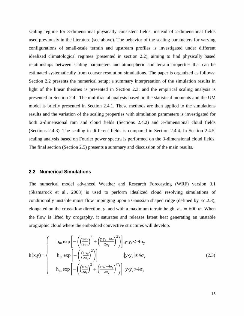
2.2 Numerical Simulations
The numerical model advanced Weather and Research Forecasting (WRF) version 3.1
(Skamarock et al., 2008) is used to perform idealized cloud resolving simulations of
conditionally unstable moist flow impinging upon a Gaussian shaped ridge (defined by Eq.2.3),
elongated on the cross-flow direction, , and with a maximum terrain height . When
the flow is lifted by orography, it saturates and releases latent heat generating an unstable
orographic cloud where the embedded convective structures will develop.
-
-
- -
-
-
-
-
-
(2.3)

14
Decay parameters and are 12.5 and 5 km respectively, and the center of the ridge is
defined at . The resulting modified Gaussian ridge is represented in Fig.
2.1a. In all simulations the horizontal resolution is 250 m and there are 70 vertical terrain-
following levels, unequally distributed over the 15 km of the domain, with vertical spacing
stretching from lower to higher levels in order to have better resolution in the region where
orographic clouds will develop. A Rayleigh damping layer is introduced in the top 5 km to
reduce spurious reflections at the top. To simplify the problem, the parameterizations for
radiation or surface and boundary layer are turned off, and the effects of earth’s rotation are also
neglected. The 3-dimensional Smagorinsky scheme is used for sub-grid turbulence closure.
Figure 2.1. Horizontal maps of topographic elevation (in meters) for simulations: a) CTL and b)
Sst10km. The inner black square represents the domain of interest where the scaling analysis
computations are performed.
15
These highly idealized simulations are based on previous works of Kirshbaum and Durran
(2005a,b) and Kirshbaum et al. (2007a,b) where the authors showed that they reproduce essential
features of observed convective bands in the Oregon Coastal Range. The model resolution is fine
enough to resolve the convective scale (see e.g. Fuhrer and Schär, 2007), and thus it is assumed
that these simulations represent the appropriate convective structures. However, there are two
important differences between the present simulations and previous work: i) the Thompson et al.
microphysics scheme (available in WRF 3.1) including cold microphysics is used in this study
instead of warm rain schemes, which may be difficult to justify in the case of orographic
precipitation simulations; ii) the large-scale orography is a finite length ridge and open boundary
conditions are used in this study for all lateral boundaries instead of a quasi-1-dimensional ridge
with periodic boundary conditions in the boundaries. Periodic boundary conditions used in
previous studies would reintroduce small-scale disturbances in the domain reinforcing certain
wavelengths, and would not allow the upstream stable flow to flow around the ridge, eventually
forcing it all to transpose the orographic barrier.
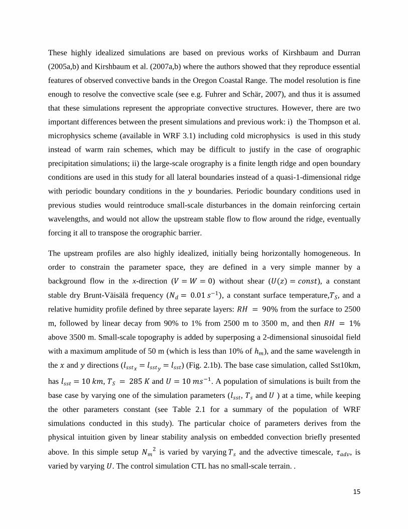
The upstream profiles are also highly idealized, initially being horizontally homogeneous. In
order to constrain the parameter space, they are defined in a very simple manner by a
background flow in the x-direction ( ) without shear ( ), a constant
stable dry Brunt-Väisälä frequency ( , a constant surface temperature, and a
relative humidity profile defined by three separate layers: from the surface to 2500
m, followed by linear decay from 90% to 1% from 2500 m to 3500 m, and then
above 3500 m. Small-scale topography is added by superposing a 2-dimensional sinusoidal field
with a maximum amplitude of 50 m (which is less than 10% of ), and the same wavelength in
the and directions ( ) (Fig. 2.1b). The base case simulation, called Sst10km,
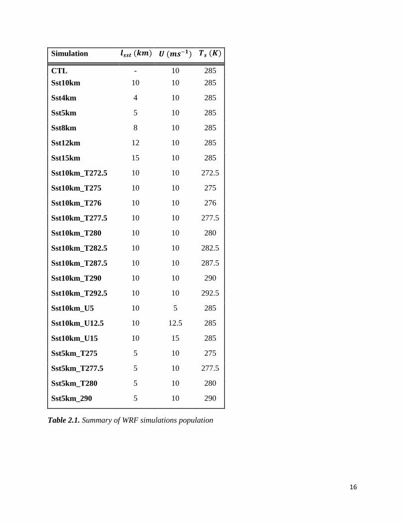
has , and . A population of simulations is built from the
base case by varying one of the simulation parameters ( , and ) at a time, while keeping
the other parameters constant (see Table 2.1 for a summary of the population of WRF
simulations conducted in this study). The particular choice of parameters derives from the
physical intuition given by linear stability analysis on embedded convection briefly presented
above. In this simple setup is varied by varying and the advective timescale, , is
varied by varying . The control simulation CTL has no small-scale terrain. .
16
Simulation
CTL - 10 285
Sst10km 10 10 285
Sst4km 4 10 285
Sst5km 5 10 285
Sst8km 8 10 285
Sst12km 12 10 285
Sst15km 15 10 285
Sst10km_T272.5 10 10 272.5
Sst10km_T275 10 10 275
Sst10km_T276 10 10 276
Sst10km_T277.5 10 10 277.5
Sst10km_T280 10 10 280
Sst10km_T282.5 10 10 282.5
Sst10km_T287.5 10 10 287.5
Sst10km_T290 10 10 290
Sst10km_T292.5 10 10 292.5
Sst10km_U5 10 5 285
Sst10km_U12.5 10 12.5 285
Sst10km_U15 10 15 285
Sst5km_T275 5 10 275
Sst5km_T277.5 5 10 277.5
Sst5km_T280 5 10 280
Sst5km_290 5 10 290
Table 2.1. Summary of WRF simulations population
17
2.3 Dynamical interpretation: linear stability analysis
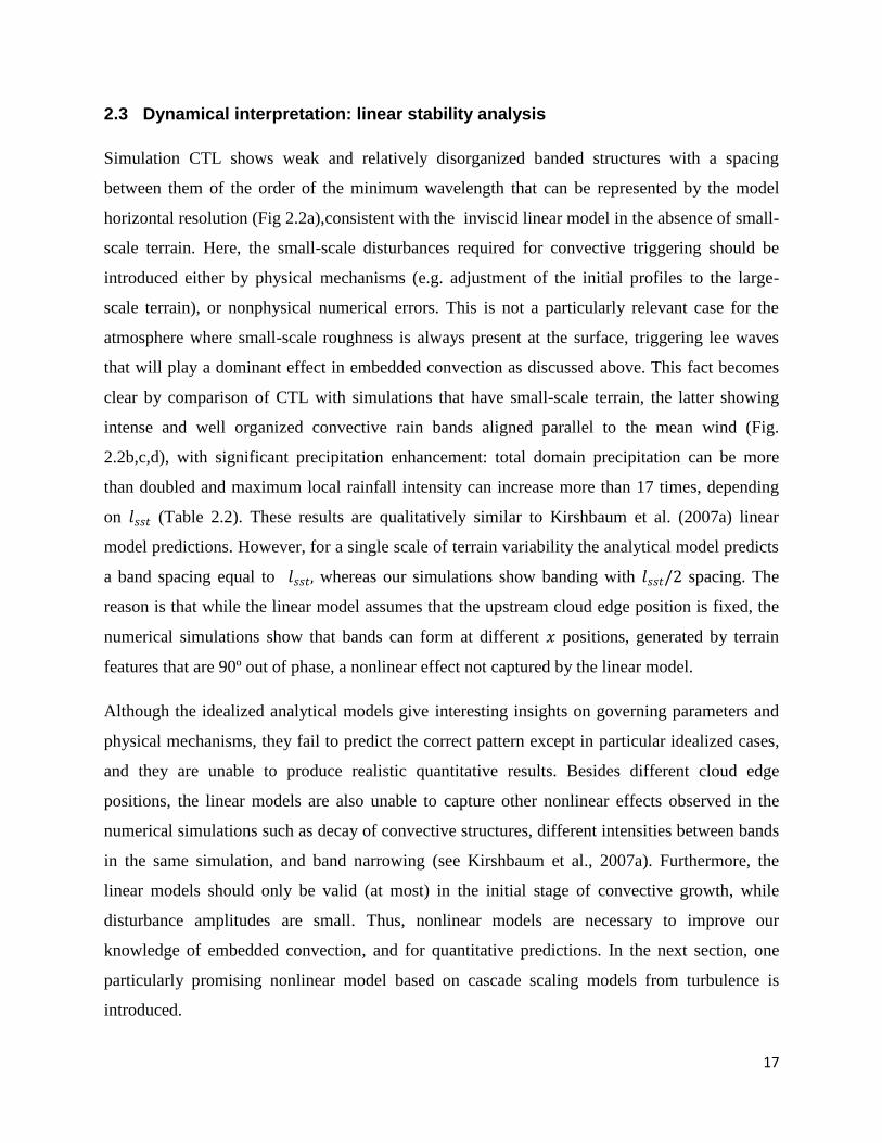
Simulation CTL shows weak and relatively disorganized banded structures with a spacing
between them of the order of the minimum wavelength that can be represented by the model
horizontal resolution (Fig 2.2a),consistent with the inviscid linear model in the absence of small-
scale terrain. Here, the small-scale disturbances required for convective triggering should be
introduced either by physical mechanisms (e.g. adjustment of the initial profiles to the large-
scale terrain), or nonphysical numerical errors. This is not a particularly relevant case for the
atmosphere where small-scale roughness is always present at the surface, triggering lee waves
that will play a dominant effect in embedded convection as discussed above. This fact becomes
clear by comparison of CTL with simulations that have small-scale terrain, the latter showing
intense and well organized convective rain bands aligned parallel to the mean wind (Fig.
2.2b,c,d), with significant precipitation enhancement: total domain precipitation can be more
than doubled and maximum local rainfall intensity can increase more than 17 times, depending
on (Table 2.2). These results are qualitatively similar to Kirshbaum et al. (2007a) linear
model predictions. However, for a single scale of terrain variability the analytical model predicts
a band spacing equal to whereas our simulations show banding with spacing. The
reason is that while the linear model assumes that the upstream cloud edge position is fixed, the
numerical simulations show that bands can form at different positions, generated by terrain
features that are 90º out of phase, a nonlinear effect not captured by the linear model.
Although the idealized analytical models give interesting insights on governing parameters and
physical mechanisms, they fail to predict the correct pattern except in particular idealized cases,
and they are unable to produce realistic quantitative results. Besides different cloud edge
positions, the linear models are also unable to capture other nonlinear effects observed in the
numerical simulations such as decay of convective structures, different intensities between bands
in the same simulation, and band narrowing (see Kirshbaum et al., 2007a). Furthermore, the
linear models should only be valid (at most) in the initial stage of convective growth, while
disturbance amplitudes are small. Thus, nonlinear models are necessary to improve our
knowledge of embedded convection, and for quantitative predictions. In the next section, one
particularly promising nonlinear model based on cascade scaling models from turbulence is
introduced.
18
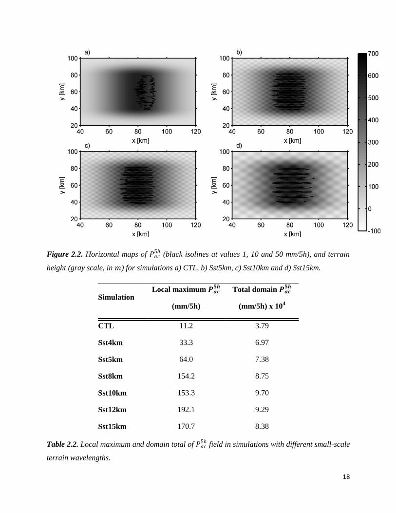
Figure 2.2. Horizontal maps of
(black isolines at values 1, 10 and 50 mm/5h), and terrain
height (gray scale, in ) for simulations a) CTL, b) Sst5km, c) Sst10km and d) Sst15km.
Simulation Local maximum
(mm/5h)
Total domain
(mm/5h) x 104
CTL 11.2 3.79
Sst4km 33.3 6.97
Sst5km 64.0 7.38
Sst8km 154.2 8.75
Sst10km 153.3 9.70
Sst12km 192.1 9.29
Sst15km 170.7 8.38
Table 2.2. Local maximum and domain total of
field in simulations with different small-scale
terrain wavelengths.

19
2.4 Empirical scaling analysis
2.4.1 The Universal Multifractal model
The existence of scale invariance in atmospheric fields is often investigated by analyzing their
statistical moments, which are expected to obey the generic multiscaling relation:
(2.4)
where represents the statistical average, is the moment order generalized to any positive real
number,
is the scale ratio, being the outer scale of the cascade (the largest scale of
variability) and the scale of the observation, or simulation. is a quantity that is on average
conserved from scale to scale in a similar way to what happens in turbulence cascade models.
The turbulent flux is non-dimensionalized and normalized, such that . In general
geophysical fields are multifractals, i.e. the exponent K is a function of q, and thus an infinity of
exponents are required to characterize the scaling behavior. However, one can use the UM
framework to model the variation of with for a conserved process, reducing the problem to
two parameters ( and ; Schertzer and Lovejoy 1987):
(2.5)
The Levy index, , defined in the interval [0,2], indicates the degree of multifractality ( for
monofractals); and the co-dimension of the mean singularity, , describes the sparseness or non-
homogeneity of the mean of the process. The moment order must be positive ( ) in this
framework.
There is no physical basis to assume that a general observable, , (e.g. wind, temperature,
rainfall, etc.) should be conserved on a scale by scale basis. In analogy with turbulence models,
we may expect that observable fluctuations, , over a distance , are related to a general
turbulent conserved flux, , by:
(2.6)

20
A third Universal Multifractal parameter is introduced in Eq. 2.6: the Hurst exponent (or
nonconservation parameter), . In a conservative process , and thus and
. But in the general case, the mean has a dependence on scale, . The other
exponent, , depends on the particular field being analyzed. Note that Eq. 2.6 is a generalization
of the classical laws of turbulence. For example, in the Kolmogorov (1941) law for turbulent
velocity fluctuations: , we have that , and . In this case
the observable (turbulent wind field, ) is not the direct result of a multiplicative cascade, that
role being reserved for the (cascade conserved) energy flux, . The cascade conserved flux can
have more complex forms that include nonlinear interactions of different fluxes, e.g. the Corsin-
Obukhov law for passive scalar advection (Obukhov, 1949; Corsin, 1951): ,
where , being the scalar variance flux. In these classic turbulence cases,
the laws relating the observable fluctuations and conserved turbulent fluxes can be obtained from
the governing dynamical equations, assuming isotropy, and via dimensional analysis. For rain
and cloud processes (which generally cannot be assumed to behave as passive scalars), the
values of and are unknown, and so is the physical nature of the conserved flux. However it is
still possible to perform scaling analysis. We start by taking the simplifying assumption =1, as
usually done in similar previous works, noticing that if is a pure multiplicative cascade then
that is also true for , although with different C1 values (e.g. Tessier et al., 1993; Stolle et al.,
2009). The next step is to remove the influence of the term. One method used for this purpose
is to rely on the absolute value of a finite difference gradient to compute the fluctuations at the
highest resolution available, (see e.g. Lavallée et al., 1993; Tessier et al., 1993):
(2.7)
The flux estimates given by Eq. 2.7 are systematically degraded to lower resolutions (lower
values of ) by spatial averaging. The Double Trace Moment (DTM) technique (e.g. Lavallée et
al, 1993) can be used subsequently to estimate and . Notice that the values of the UM
parameters estimated from data generated by numerical models are not the same as the ones
obtained from observations due to cascade cutoff by model resolution and model domain, but it
is possible to convert between them (Stolle et al., 2009). Nevertheless, incorrect representation
of physical processes in the models cannot be corrected. In the present work we aim only to
21
investigate the variation of the UM parameters in numerical simulations with similar setup, so no
conversion is required.
Spectral analysis can also be used to investigate the behavior of a field over a wide range of
scales. The spatial Fourier power spectrum, , is computed by multiplying the 2-
dimensional fast Fourier transform of a field by its complex conjugate, where and are the
wavenumber components. The power spectrum is then averaged angularly about
to yield what is usually called isotropic power spectrum , with
.
Spatial scaling invariance manifests itself as log-log linearity of the power spectrum in space:
(2.8)
Where is the spectral exponent and the addition of -1 in the exponent is required due radial
averaging is phase space (e.g. Turcotte, 1992; Lovejoy et al., 2008b). Least square regression is
used to estimate from a log-log plot of against .
The spectral exponent is related to the UM parameters by (Tessier et al., 1993):
(2.9)
Finally we estimate from the slope of the log-log plot of the first order structure function
against the lag, as described by Harris et al. (2001), Nykanen (2008) and Lovejoy et al.
(2008a,b).
2.4.2 Scaling in simulated 2D fields
The empirical scaling analysis described above is applied to surface accumulated precipitation
spatial fields over 5 hour simulations,
. Here the constant value domain length) was
used for the cascade outer scale, . Changing the chosen value of has no effect on the
estimated value of the slope of the fitted lines, i.e. on and respective UM parameter
estimation. Fig. 2.3a-c shows log-log plots of against for
fields for three different
simulations. The lines are only fitted to the range of scales that are well resolved by the model,
i.e. larger than and smaller than about . For the linear
fits are good implying that statistical scale invariance predicted by Eq. 2.4 is a good

22
representation, and that there are no characteristic scales or scale breaks for the considered
ranges of and (from ~1 to ~ 20 km). This range of is similar to the ones found in literature
for similar analysis (e.g Douglas and Barros, 2003; Lovejoy et al., 2008a,b; Nykanen, 2008; de
Lima and de Lima, 2009). Some simulations show ersistent deviations from linear behavior at
particular scales, but the relation between these scales and varies between simulations,
suggesting that the small-scale terrain wavelength is not (statistically) a characteristic scale in the
rain fields. The same spatial scaling analysis was repeated for the
fields resulting from all
simulations in Table 2.1, all of them showing the same robust scaling behavior (linear relations).
Figure 2.3. Relationship between and for different values of q. is computed from
from simulation a) Sst5km, b) Sst10km, c) Sst15km. The scales considered on the analysis are
ark by ‘o’ whi ‘x’ arks th ones not considered. The plots are on a log-log scale.
23
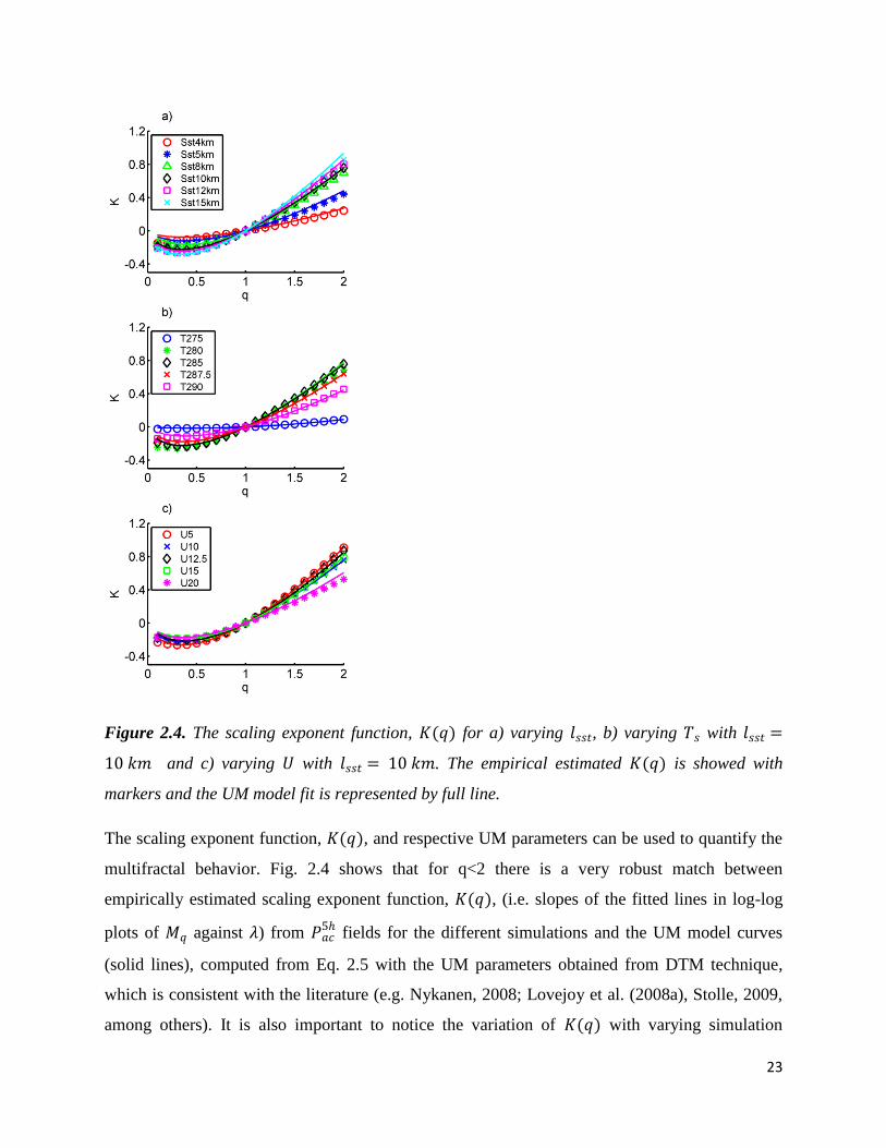
Figure 2.4. The scaling exponent function, for a) varying , b) varying with
and c) varying with . The empirical estimated is showed with
markers and the UM model fit is represented by full line.
The scaling exponent function, , and respective UM parameters can be used to quantify the
multifractal behavior. Fig. 2.4 shows that for q<2 there is a very robust match between
empirically estimated scaling exponent function, , (i.e. slopes of the fitted lines in log-log
plots of against ) from
fields for the different simulations and the UM model curves
(solid lines), computed from Eq. 2.5 with the UM parameters obtained from DTM technique,
which is consistent with the literature (e.g. Nykanen, 2008; Lovejoy et al. (2008a), Stolle, 2009,
among others). It is also important to notice the variation of with varying simulation
24
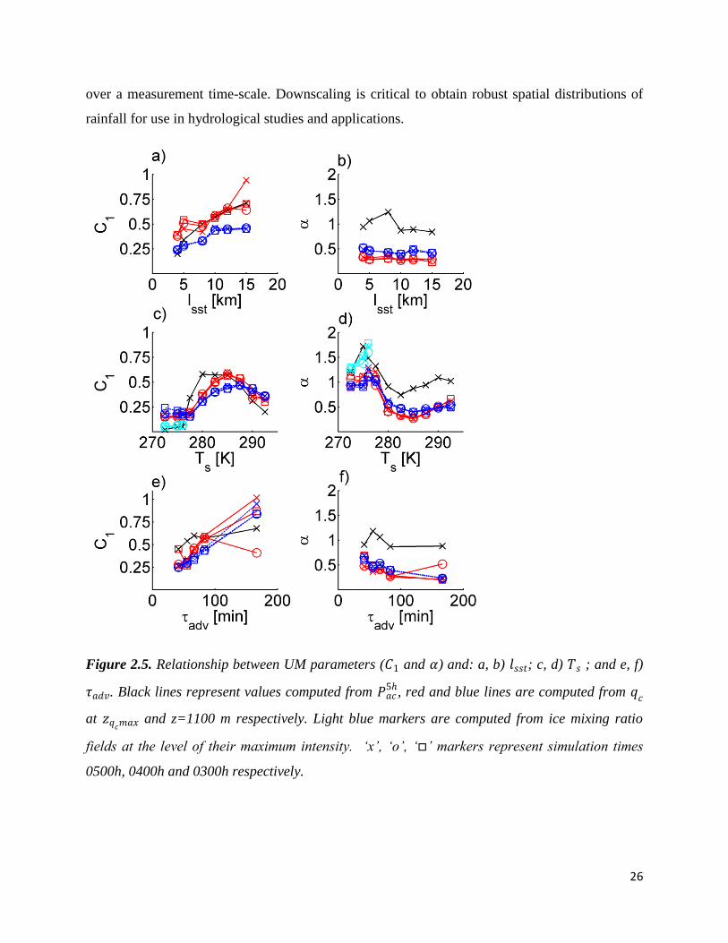
attributes ( , and ). This variation is quantified in Fig. 2.5 (black line) using and ,
which display a complex nonlinear variation with simulation attributes. A particularly
remarkable feature is the abrupt transition in both UM parameters for between 275K and
285K. The transition has a physical correspondence when interpreted against the spatial rainfall
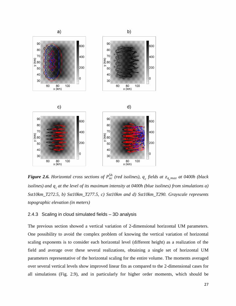
patterns (red lines in Fig. 2.6), capturing the evolution from terrain-following (more stratiform)
and less intense rainfall fields in the colder simulation cases to well organized and intense bands
for simulations at intermediate temperatures. For warmer simulations the rainfall pattern changes
again to more intense but less organized (more cellular) convective features (Fig. 2.6d), and the
UM parameters also show variation (Fig. 2.5c and d). These differences in convective dynamics
have important effects in rainfall intensities and patterns leading to high localized rainfall
accumulation values (Table 2.3, and see also Kirhsbaum and Durran, 2005b and Fuhrer and
Schär, 2007).
The same analysis was performed on instantaneous horizontal cross sections of cloud water
mixing ratio, , at two different levels (the height of maximum intensity, and z=1100
m) after 3, 4 and 5 hours of simulation, corresponding to the mature stage when the convective
structures are fully grown. Fig. 2.7 illustrates the robust scaling of moments of fields at
for three different simulations. The same behavior is found for cloud fields in all simulations in
Table 2.1, at all the analyzed times and heights. The UM parameters computed from also
display complex nonlinear variation with simulation properties (red line at and blue at
z=1100 m in Fig. 2.5). In particular the transition between colder and warmer cases is again
clear. Both and show similar values at the different times, due to the quasi-stationary state
of the convective structures that is attained in these simulations. Comparison of the scaling
parameters computed from fields at different vertical levels shows vertical variation of both
UM parameters, although the shape of the curve is largely preserved. Notice that the level
varies between simulations and with time, and it can sometimes capture different structures and
cause significant variations of the parameters. This explains some values that seem to fall outside
the curves: for example the value of for Sst15km at 0500h computed from at is
quite different from the one at 0400h, which is easily understood by examining Fig. 2.8: in
Sst10km the level crosses the core of the cloud band, the same happening for Sst15km at
0400h, while at Sst15km at 0500h it is actually crossing a region of instabilities that has formed
25
on the top region of the band, resulting in a different horizontal pattern and associated scaling
parameters. The large variation in for the largest advective timescale at different times
has a similar explanation.
Simulation
Local maximum
of
(mm/5h)
Total domain
(mm/5h) x 104
Local
maximum of
(g/kg)
Local
maximum of
(g/kg)
Sst10km_T272.5_WR 0.00 0.00 0.53 -
Sst10km_T272.5 1.90 4.79 0.24 0.11
Sst10km_T275 1.75 3.63 0.27 0.13
Sst10km_T276 1.80 3.05 0.33 0.13
Sst10km_T277.5 0.33 0.07 0.71 0.00
Sst10km_T280 23.77 1.20 1.10 0.00
Sst10km_T282.5 83.72 2.83 1.34 0.00
Sst10km 153.28 4.68 1.49 0.00
Sst10km_T287.5 143.06 9.20 1.57 0.83
Sst10km_T290 214.45 31.59 1.79 2.13
Sst10km_T292.5 258.87 76.43 2.18 5.25
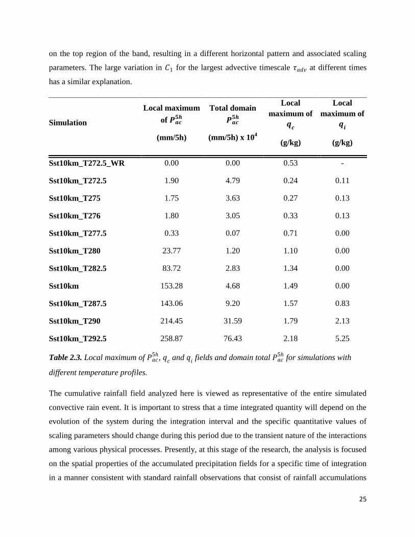
Table 2.3. Local maximum of
, and fields and domain total
for simulations with
different temperature profiles.
The cumulative rainfall field analyzed here is viewed as representative of the entire simulated
convective rain event. It is important to stress that a time integrated quantity will depend on the
evolution of the system during the integration interval and the specific quantitative values of
scaling parameters should change during this period due to the transient nature of the interactions
among various physical processes. Presently, at this stage of the research, the analysis is focused
on the spatial properties of the accumulated precipitation fields for a specific time of integration
in a manner consistent with standard rainfall observations that consist of rainfall accumulations
26
over a measurement time-scale. Downscaling is critical to obtain robust spatial distributions of
rainfall for use in hydrological studies and applications.
Figure 2.5. Relationship between UM parameters ( and ) and: a, b) ; c, d) ; and e, f)
. Black lines represent values computed from
, red and blue lines are computed from
at and z=1100 m respectively. Light blue markers are computed from ice mixing ratio
fi s at th v of th ir axi u i t sity. ‘x’, ‘o’, ‘ ’ ark rs r r s t si u atio ti s
0500h, 0400h and 0300h respectively.
27
Figure 2.6. Horizontal cross sections of
(red isolines), fields at at 0400h (black
isolines) and at the level of its maximum intensity at 0400h (blue isolines) from simulations a)
Sst10km_T272.5, b) Sst10km_T277.5, c) Sst10km and d) Sst10km_T290. Grayscale represents
topographic elevation (in meters)
2.4.3 Scaling in cloud simulated fields – 3D analysis
The previous section showed a vertical variation of 2-dimensional horizontal UM parameters.
One possibility to avoid the complex problem of knowing the vertical variation of horizontal
scaling exponents is to consider each horizontal level (different height) as a realization of the
field and average over these several realizations, obtaining a single set of horizontal UM
parameters representative of the horizontal scaling for the entire volume. The moments averaged
over several vertical levels show improved linear fits as compared to the 2-dimensional cases for
all simulations (Fig. 2.9), and in particularly for higher order moments, which should be

28
explained by the larger data sample size considered. Like in the 2-dimensional case, some
persistent deviations are identifiable but they have smaller amplitudes, and the particular scales
for each simulation between 2- and 3-dimensional cases are different, providing support to the
notion of absence of characteristic scales. The presence of scaling behavior for the entire volume
implies that concurrent spatial structures (e.g. band core region, instabilities at the top of the
bands, clouds that form downstream of the large scale orography, among others, Fig. 2.8) fall in
the same average horizontal scaling regime. The scaling behavior in the vertical direction is not
investigated here due to data limitations associated with the limited number of vertical levels in
the model (see section 2.2) together with the fact that we are looking at instantaneous realizations
of fields rather than ensemble average statistics. But in other cases it could be investigated using
a different set of UM parameters to describe anisotropy between horizontal and vertical
directions (see e.g. Lovejoy et al., 1987, Lazarev et al., 1994; Radkevich et al., 2007).
As in the 2-dimensional case, the UM parameters vary with mean atmospheric and terrain
properties (Fig. 2.10). Fig. 2.10a shows decreasing with while Fig. 2.10b shows there is
little variation of with . Figs. 2.10c and d show the abrupt transitions in both scaling
parameters with changes in , further providing support for this result. Recall that in these
idealized simulations the temperature profiles and cloud layer stability are determined by .
However, in more realistic profiles this will not generally be true. Linear stability analysis
suggests that a good alternative is to characterize the atmospheric environment using a (spatial)
average value. This average is computed at each time instant and only from points that
exceed a fixed (arbitrary) threshold (e.g. 0.01 g/kg) as it is defined only in saturated regions.
Figures 2.11a and 2.11b show that the abrupt transition corresponds to the transition between the
stable ( ) and unstable (
) cases. For larger negative values,
there is a break in variability of the UM parameters for small changes in ,
particularly clear in C1. This behavior poses an intriguing question as to the character of the
underlying physics and of this flow transition for highly unstable flows, not unlike the transition to high
Reynolds numbers in the case of fully-develepod turbulence turbulence . The fields with the strongest
instability values are not necessarily the warmer ones as defined by the initial conditions, as the
average value can be significantly altered by the release of latent heating or due to the
presence of downstream stable clouds and other features.

29
Figure 2.7. Relationship between and for different values of q. is computed from at
at 0400h for simulation a) Sst5km, b) Sst10km and c) Sst15km. The scales considered on
th a a ysis ar ark by ‘o’ whi ‘x’ arks th o s ot o si r . h ots ar o a o -
log scale.
To capture the effect of space-time co-localization of moist instability release and moist
processes, can be multiplied by a measure of the cloud fraction, , defined here by the
ratio of number of grid points that exceed the chosen threshold to the total number of points.
This transformation gives a measure of the overall realized moist instability at a given point in
time, and provides a physically-based framework to arrange the simulations in the order of
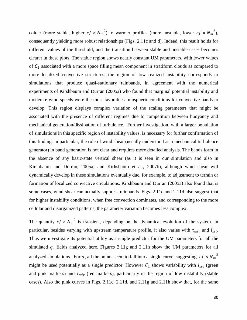
30
colder (more stable, higher ) to warmer profiles (more unstable, lower
),
consequently yielding more robust relationships (Figs. 2.11c and d). Indeed, this result holds for
different values of the threshold, and the transition between stable and unstable cases becomes
clearer in these plots. The stable region shows nearly constant UM parameters, with lower values
of associated with a more space filling mean component in stratiform clouds as compared to
more localized convective structures; the region of low realized instability corresponds to
simulations that produce quasi-stationary rainbands, in agreement with the numerical
experiments of Kirshbaum and Durran (2005a) who found that marginal potential instability and
moderate wind speeds were the most favorable atmospheric conditions for convective bands to
develop. This region displays complex variation of the scaling parameters that might be
associated with the presence of different regimes due to competition between buoyancy and
mechanical generation/dissipation of turbulence. Further investigation, with a larger population
of simulations in this specific region of instability values, is necessary for further confirmation of
this finding. In particular, the role of wind shear (usually understood as a mechanical turbulence
generator) in band generation is not clear and requires more detailed analysis. The bands form in
the absence of any basic-state vertical shear (as it is seen in our simulation and also in
Kirshbaum and Durran, 2005a; and Kirhsbaum et al., 2007b), although wind shear will
dynamically develop in these simulations eventually due, for example, to adjustment to terrain or
formation of localized convective circulations. Kirshbaum and Durran (2005a) also found that is
some cases, wind shear can actually suppress rainbands. Figs. 2.11c and 2.11d also suggest that
for higher instability conditions, when free convection dominates, and corresponding to the more
cellular and disorganized patterns, the parameter variation becomes less complex.
The quantity is transient, depending on the dynamical evolution of the system. In
particular, besides varying with upstream temperature profile, it also varies with and .
Thus we investigate its potential utility as a single predictor for the UM parameters for all the
simulated fields analyzed here. Figures 2.11g and 2.11h show the UM parameters for all
analyzed simulations. For , all the points seem to fall into a single curve, suggesting
might be used potentially as a single predictor. However shows variability with (green
and pink markers) and (red markers), particularly in the region of low instability (stable
cases). Also the pink curves in Figs. 2.11c, 2.11d, and 2.11g and 2.11h show that, for the same
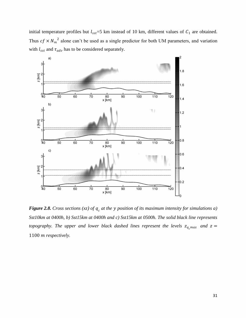
31
initial temperature profiles but =5 km instead of 10 km, different values of are obtained.
Thus alone can’t be used as a single predictor for both UM parameters, and variation
with and has to be considered separately.
Figure 2.8. Cross sections (xz) of at the position of its maximum intensity for simulations a)
Sst10km at 0400h, b) Sst15km at 0400h and c) Sst15km at 0500h. The solid black line represents
topography. The upper and lower black dashed lines represent the levels and
respectively.
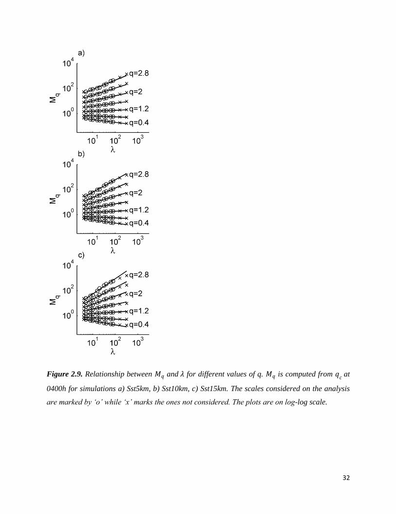
32
Figure 2.9. Relationship between and for different values of q. is computed from at
0400h for simulations a) Sst5km, b) Sst10km, c) Sst15km. The scales considered on the analysis
ar ark by ‘o’ whi ‘x’ arks th o s ot o si r . h ots ar o o -log scale.
33
Figure 2.10. and computed from 3-dimensional averages of horizontal fluctuations
against: a, b) , c, d) and e, f) . Black lines represent values computed from
. Green,
blue and red lines are computed from . The light blue markers lines are computed from . ‘x’,
‘o’ a ‘ ’ ark rs r r s t si u atio ti s 0500h, 0400h a 0300h, respectively.
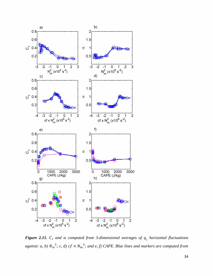
34
Figure 2.11. and computed from 3-dimensional averages of horizontal fluctuations
against: a, b) ; c, d)
; and e, f) CAPE. Blue lines and markers are computed from
35
simulations with varying and = 10 km, pink from simulations with varying and = 5
km, red for varying and green for varying . Plots g, h) show and against
for all simulations. Black markers in plots g) and h) represent simulation Sst10km (i.e. the base
as ). ‘x’, ‘o’ a ‘ ’ ark rs r r s t si u atio ti s 0500h, 0400h a 0300h r s tiv y.
As mentioned earlier, Perica and Foufoula-Georgiou (1996) found a linear dependency of
statistical scaling parameters on another atmospheric stability measure, the Convective Available
Potential Energy (CAPE), for a small number of rainfall fields of selected convective storms
over relatively flat topography. This result was tested in our simulated fields which have a wider
range of values, and a more complex nonlinear relation was obtained (Fig. 2.11 e and f).
Compared to , the use of has the disadvantage that the stable range of the profiles is
ambiguous ( for all stable cases), which presents a problem unless UM parameters
were shown to be constant for all stable cases. Nevertheless, note that the unstable/stable
transition of the parameters is still clear as goes to zero, as well as the complex nonlinear
behavior for the small magnitude instability values - the banded cases - and again less complex
behavior for higher magnitude instability values - cellular disorganized cases. This is consistent
with Kirshbaum and Durran (2005b) who proposed that the distinction between more banded and
cellular cases is related to enhanced susceptibility to free convection, with larger CAPE implying
more cellular structures. They suggest that Convective INhibtion ( ) could be an important
parameter as well, but all our simulations have very small values of and are not suitable for
such analysis.
2.4.4 Relations between different scaling fields
In both 2- and 3-dimensional analysis, UM parameters computed from
and show clear
relations for certain ranges of simulation properties, either in the shape of the variation curve in
Figs. 2.5a,c,d and Figs. 2.10ac,d,e, or for the exact values of the parameter, as can be seen for
example in Fig. 5a for computed from at for km and C1 computed from
=1100 m for smaller ( also in Fig. 2.5c, see the computed from at for
, and in Fig. 2.11c for ). For the 2-dimensional analysis these relationships
depend on the chosen vertical level, sometimes best relating to the level of maximum intensity,
36
sometimes to some other level, which makes its use difficult in practical applications, further
supporting the 3-dimensional analysis.
Figs. 2.5c,d and 2.10c,d show that for colder simulations ( ) both UM parameters
computed from
are very similar to the ones computed from ice phase (snow+ice+graupel)
mixing ratio fields, , which is particularly remarkable in the 3-dimensional analysis. The role
of cold microphysics on precipitation processes is also clear in simulation Sst10km_T272.5_WR
(which is exactly the same as in Sst10km_T272.5, except that the Kessler warm rain scheme is
used in WRF and ice microphysics is turned off). The simulation with warm rain processes only
produces a cloud pattern similar to the one including cold microphysics, but it yields zero
(Table 2.3). This result is strengthened by the fact that below the values of precipitation
intensity and increase with decreasing temperature (Table 2.3). Finally, it is also apparent in
Fig. 6a that for the colder case there is a clear relation between the
(red line) and (blue
line) patterns, while the (black line) seems to be more closely related to the underlying
topography (grey scale). If the temperature is slightly raised, both and
go to zero (Fig.
2.6b and Table 2.3). If the temperature is raised further, well organized cloud bands form with a
clearly associated
pattern and no ice phase (Fig. 2.6c). Besides varying , changing
also changes the amounts of water in each phase and the vertical structure of the clouds,
particularly the cloud depth (Fig. 2.12), which the linear theory also predicts as being an
important parameter in embedded convection. For the warmer cases considered here, the cloud
depth growths enough so that ice processes become important again (blue lines in Fig. 2.6d and
Table 2.3), but the precipitation pattern now seems to be more related to (Fig. 2.6d). In these
warmer cases, the parameter from
seems to relate better to while seems to relate
better to (Fig. 2.10c,d). Overall, these results suggest that scaling of the simulated total
precipitation fields is a complex function of the scaling of several other fields including water
mixing ratio in the different phases, and probably also small-scale terrain spectra and . That
is, the scaling of the integral precipitation fields reflects the underlying governing physical
processes, which change with time and space as weather systems evolve and propagate over
complex terrain.

37
Figure 2.12. Vertical profiles of at the position of their maximum intensity at 0400h, for
simulations with and varying .
2.4.5 Spectral Analysis
The isotropic power spectra, described in Section 2.4.1, can also be used to investigate the spatial
scaling of horizontal fields. Here we average the spectra of instantaneous fields over several
vertical levels, similar to what was done in Section 2.4.3 for moment scaling analysis. Figure
2.13 shows three examples of log-log power spectra (black lines) computed at simulation hour
0400: at the bottom for a colder stable case (Sst10km_T275), in the middle for an intermediate
banded case (Sst10km), and at the top for a warmer more disorganized convective case
(Sst10km_T292.5). Only the scales well resolved by the model are considered (and represented),
assumed here to be larger than (limited by model resolution). It is important to keep in mind
that Fourier analysis has the implicit requirement (assumption) of an infinite domain, and clearly
here, as in general in all applications of Fourier analysis to digital data, we are limited by the
domain size of the grid, to which the analysis is quite sensitive. It was found that the scale range
we considered above L0/4 is too large based on the lack of symmetry of the domain, and the
upper boundary of the range was reduced to a value . Outside this range, we do not have
enough information on the power spectrum of the field.
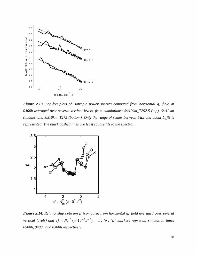
38
Figure 2.13. Log-log plots of isotropic power spectra computed from horizontal field at
0400h averaged over several vertical levels, from simulations: Sst10km_T292.5 (top), Sst10km
(middle) and Sst10km_T275 (bottom). Only the range of scales between and about is
represented. The black dashed lines are least square fits to the spectra.
Figure 2.14. Relationship between (computed from horizontal field averaged over several
vertical levels) and . ‘x’, ‘o’, ‘ ’ ark rs r r s t simulation times
0500h, 0400h and 0300h respectively.

39
The black dashed lines in Fig. 2.13 are least-square fits to the considered range of scales
(wavenumbers) of the power spectrum. There is a clear mean linear trend (scaling) in the log-log
power spectra, with R2 values for the least-square fits always above 0.90. Peaks in the power
spectra, particularly evident in the intermediate banded case spectrum (middle spectra in Fig.
2.13), are consistent with harmonics resulting from the banded pattern. This behavior is
expected when analyzing single realizations of cloud fields (e.g. Harris et al., 2001), and more so
for events over complex terrain when orographic forcing is dominant (e.g. see scaling analysis in
Barros et al. 2004). The scaling analysis was repeated here for all the simulations with
and varying , all of them showing a mean linear trend in the log-log power spectra.
Fig. 2.14 shows that the variation of fitted values of with displays similar transitions
to the ones found for UM parameters, between stable/unstable cases and banded/disorganized
convection. The location of the stable/unstable transition now seems to have been shifted to
values slightly lower than . For numerical modeling parameterizations or downscaling,
the exact location of this transition should be determined using a large data base of realistic
simulations. Yet, the existence of such transition alone, which is supported by both spectra and
moment scaling analysis and agrees with expected physical behavior such as for example the
Richardson number criteria in boundary layer stability analysis, is an important finding in itself.
The colder stratiform cases show some spread in values that was not found in the UM
parameters, including an unphysical value. It should be taken into consideration these
cases have shallower clouds (Fig. 2.12), which imply fewer levels of data for computation, along
with low intensities of cloud fields, making them susceptible to computational uncertainty in the
spectral exponent, adding to the limitations in the spectral analysis. The highly idealized
topography with a superposed 2-dimensional sinusoidal field used in the simulations here was
designed to replicate and build upon previous works that used linear theory to investigate the
development of orographic convection, and is not scaling. The structure of stratiform (terrain
following) and orographically triggered convective fields is very influenced by the properties of
the topographic elevation (e.g. Barros and Lettenmaier, 1994; Kirshbaum and Durran, 2004;
Barros et al., 2004), and therefore a linkage between their scaling properties should exist. Follow
up work, with realistic terrain should give further insight into this question.
40
Theoretically (isotropic) wind speed and passive scale advection in turbulent processes has
for 3-dimensional turbulence, and 3 for 2-dimensional turbulence. However cloud
fields in convective turbulence should not be treated as passive scalars due to strong nonlinear
effects such as latent heating release, entrainment, and active thermodynamics and microphysical
processes, and therefore these theoretical results cannot be expected to hold. Additionally these
theories assume isotropy between horizontal and vertical directions which is not the case in the
atmosphere.
2.5 Summary and discussion
Linear stability analysis reveals that embedded convective structures are the result of unstable
growth of small-scale disturbances, which should be very important in determining the
predictability of orographic precipitation. They also suggest the governing role of parameters
such as atmospheric stability, advective timescale, small-scale terrain spectra and cloud depth.
The results from idealized numerical simulations of orographic convective precipitation
qualitatively agree with these predictions. Particularly, they show that the representation of
small-scale terrain (and associated lee waves) plays a very important role for these events,
controlling the band spacing and significantly enhancing the convective intensity and rainfall
amounts. But these simple models are unable to do any quantitative predictions or even predict
the correct pattern (except in very particular cases) due to the presence of nonlinear effects, and
alternative nonlinear models are required.
As pointed out by Schertzer and Lovejoy (1992), the contributions of small-scale activity to
much larger scales are non-negligible, and indeed the corresponding variability has the most
extreme behavior which explains in part the reason why multifractals have been successful on
the study of extreme events. In fact several previous works reported statistical multiscaling
behavior to be a very general property of geophysical fields (including rain and clouds),
providing a convenient alternative framework due to its theoretical simplicity, its ability to
handle nonlinear dynamics over very wide range of scales, its potential for downscaling
applications and the fact that the convective events studied here are a particular kind of turbulent
flow and hence a statistical approach to the problem is appropriate. This multiscaling behavior
holds for statistical moments and isotropic power spectra of the simulated rain and cloud fields in

41
the considered range of scales (~1km to ~ 20 km). The Universal Multifractal model reproduces
quite well the empirical estimates of the horizontal scaling exponent function, , and can be
used to quantify the multiscaling behavior of the fields. Analysis of single horizontal sections of
cloud fields revealed variation of the scaling parameters with vertical position. We argue that if
we use an average over several horizontal sections at different vertical levels, we obtain
estimates for the horizontal parameters of the entire volume, while the vertical structure should
be represented by a different set of (vertical) scaling parameters. This transient 3-dimensional
anisotropic scaling framework seems to be a promising starting point to investigate relations
between the statistical and physical properties and perform downscaling for mesoscale events.
Results from both 2- and 3-dimensional approaches revealed significant variations of and
respective UM parameters with small-scale terrain spectra, atmospheric stability and advective
timescale. Therefore, the representation of sub-grid scale variability of cloud and rainfall fields
using statistical multifractal diagnostics would intrinsically depend not only on the properties of
the field itself, but also on particular geographic location and atmospheric conditions, bringing
the necessity of developing relationships to predict the scaling parameters from coarse grid
atmospheric data and terrain spectra. However, the results also suggest that the development of
such relationships is far from being trivial because they appear to involve complex nonlinear
behavior.
A particularly robust behavior found here is the abrupt transition in the UM parameters between
stable and unstable cases, which has a clear physical correspondence as a transition from a more
stratiform to a more organized (banded) convective regime. This behavior is also found in the
spectral exponent . Another instability measure, CAPE, also seems to be a good predictor, but
it is unable to distinguish between the different stable cases and CIN might have to be used in
conjunction. also has the advantage of allowing a linkage with the analytical models where
it appears explicitly, which is not so clear for CAPE. It was also found that the scaling of the
surface accumulated precipitation field (usually an important field to be parameterized and
downscaled) is a complex function of the horizontal scaling of several other fields such as water
mixing ratios in the different phases and probably and .
The scaling of the power spectrum can be taken advantage to perform stochastic spatial
downscaling (disaggregation) of instantaneous rain and cloud field (see e.g. Bindlish and Barros,

42
1996 and 2002; or Rebora et al., 2006). The present work suggests that scaling parameters could
be computed from known large scale measures (such as stability and terrain spectra). Although
the focus of spectral analysis is on second order statistics, and hence the scaling behavior at other
orders is neglected by this type of downscaling approach, the time dependency of the scaling
parameters is introduced by the temporal evolution of the atmospheric conditions, and the
usually small time step used in numerical simulations can be advantageous to achieve a high
temporal representation. Further improvements could include scaling constraints using higher-
order moments.
Finally, it is important to point out some limitations of our study. In order to investigate the
dependence of the multifractal properties on mean properties, a limited range of highly idealized
simulations are used where we can control the mean atmosphere with a small number of
simulation parameters. Because our work suggests a transient dependence of the scaling on mean
properties, the analysis is performed on instantaneous fields, rather than ensemble averages,
which increases the volume of data necessary for analysis. Horizontal isotropy is assumed, and it
is important to stress that the issue of existence of horizontal anisotropy must be tackled in the
future. The solutions show robust horizontal scaling even though the only external forcing is a
very simple terrain with poor scaling and the initial conditions are horizontally homogeneous. In
realistic cases, the atmosphere and terrain forcing will themselves be scaling, which might
influence the scaling of the solutions. Models such as WRF involve many subgrid scale
parameterizations which vary among model configurations. Here we use parameterizations only
for subgrid turbulence closure and microphysical processes. Whether these parameterizations
introduce unphysical scaling behavior in the models at resolved scales, and whether the scaling
depends on the particular chosen parameterizations are legitimate questions. Furthermore, in the
real atmosphere there are many other effects not considered here such as radiation, earth rotation,
surface and boundary layer effects which might introduce further complications and influence
the scaling. In this study, however we spell out unambiguously what processes are resolved or
not, and there is general a body of literature that shows that the resolution adopted can resolve
explicitly dominant convective structures (see for example Fuhrer and Schär, 2007). In fact, as
pointed out in Section 2.2, our simulations are based on previous work where the authors showed
that they reproduce the essential features of the observed convective structures in the Oregon
Coastal Range. Harris et al. (2001) compared the scaling observed and model produced
43
precipitation fields at 3-km resolution, finding an encouragingly similar behavior at scales above
5 times the resolution (i.e. 15 km). Although they simulated realistic cases with different model
and parameterizations than here, the model is based on the same governing equations. Our
assumption here is that our simulations, based on nonlinear, compressible and non-hydrostatic
Navier-Stokes equations coupled with the thermodynamics equations in the WRF model under
the specified forcing conditions represent the key physical processes of interest and that the
multifractal parameters can be used to describe the behavior of the simulated system in the
explicitly well resolved scales. It is important to stress that the fields resulting from numerical
simulations should reproduce the scaling in geophysical observations if they are to be realistic.
Furthermore, we apply multifractal analysis not as means to find universal parameters that will
exhibit consistency, though that could be a result, but rather as a mathematical model can
capture, any given scale, variability that reflects a large dynamical range of the phenomena
determined by the long range dependencies. Thus, what is consistent is the model used to
describe variability; we then make use of the multifractal model parameters as metrics that can
help interpret model dynamics and thermodynamics in a systematic way. The presence of an
underlying multifractal behavior is robustly supported by the evidence presented: a clear mean
linear trend in the spectral analysis in conjunction with the robust scaling in the moment analysis,
which is less sensitive to the data limitations and reveals robust scaling behavior up to orders of
about 2, as it is typically found in atmospheric fields and reported in literature consistent with the
scope of the present manuscript.
Although much insight was gained into scaling dependencies, particularly the presence of
transient dependence of scaling parameters on mean conditions found here, an investigation on
observational atmospheric data and realistic numerical simulations is warranted, along with
further support to whether numerical weather prediction models are able to reproduce, at least to
some extent, the multifractal properties of simulated fields and what is the effect of the particular
parameterizations chosen on the scaling. This is currently ongoing work.
Acknowledgements
The authors would like to thank three anonymous referees for their comments and suggestions
which helped to significantly improve the manuscript. This research is supported by the
Portuguese Foundation for Science and Technology (FCT) under grants SFRH/BD/61148/2009
44
and PTDC/CTE-ATM/119922/2010, and NASA grant NN1010H66G and NSF grant EAR-
0711430 with the second author.
45
3 Transient Stochastic Downscaling of Quantitative
Precipitation Estimates for Hydrological Applications†
Abstract
Rainfall fields are heavily thresholded and highly intermittent resulting in large areas of zero
values. This deforms their stochastic spatial scale-invariant behavior, introducing scaling breaks
and curvature in the spatial scale spectrum. To address this problem, spatial scaling analysis was
performed inside continuous rainfall features (CRFs) delineated by applying cluster analysis. The
results show that CRFs from single realizations of hourly rainfall display ubiquitous multifractal
behavior that holds over a wide range of scales (from km up to 100’s km). The results
further show that the aggregate scaling behavior of rainfall fields is intrinsically transient with
the scaling parameters explicitly dependent on the atmospheric environment. These findings
provide a framework for robust stochastic downscaling, bridging the gap between spatial scales
of observed and simulated rainfall fields and the high-resolution requirements of
hydrometeorological and hydrological studies.
Here, a modified fractal downscaling algorithm is presented and applied to generate 7 years of
stochastically downscaled hourly rainfall products from radar derived StageIV (~4km grid
resolution) quantitative precipitation estimates (QPE) over the Integrated Precipitation and
Hydrology Experiment (IPHEx) domain in the southeast USA. The methodology can produce
large ensembles of statistically robust high-resolution fields without additional data or any
calibration requirements, conserving the coarse resolution information and generating coherent
small-scale variability and field statistics, hence adding value to the original fields. Moreover, it
is computationally inexpensive enabling fast production of high-resolution rainfall realizations
† Nogueira
(1,2), M. and Barros
(2), A. P., 2014: Dynamical Downscaling of Quantitative
Precipitation Estimation for Hydrological Predictions in the Southern Appalachians. Submitted
to J. of Hydrology
(1) CGUL-IDL, University of Lisbon, Portugal.
(2) Duke University, Durham, North Carolina, U.S.A.
46
with latency adequate for forecasting applications. When the transient nature of the scaling
behavior is considered, the results show a better ability to reproduce the statistical structure of
observed rainfall compared to using fixed scaling parameters derived from ensemble mean
analysis.
The value of the downscaled products is demonstrated through hydrological simulations of two
distinct storm events in the Southern Appalachians, a winter storm that caused multiple
landslides and a summer tropical event that caused flashfloods. The simulations are forced by the
entire span of plausible fractally downscaled rainfall fields at two distinct resolutions (1km and
250m). The results show very good skill against the observed streamflow, especially with regard
to the timing and peak discharge of the hydrograph, and the accuracy is enhanced by increasing
the target downscaling resolution from 1 km to 250 m. Probabilistic simulations of both events
capture the observed behavior indicating that the proposed CRF-based stochastic fractal
interpolation provides a generalized framework for producing fast and reliable probabilistic
forecasts and their associated uncertainty for extreme events and risk management of
hydrometeorological hazards , as well as long-term hydrologic modeling.
3.1 Introduction
Heavy rain events over mountainous terrain present a great challenge for forecasters and are the
leading cause of natural hazards including flashfloods, shallow landslides and debris flows.
Predictability of these events depends on access to precipitation products at spatial and temporal
resolutions finer than the scales currently resolved by the Numerical Weather Prediction (NWP)
models, or the observations used to produce Quantitative Precipitation Estimates (QPE) (e.g.
ground-based radar). Consequently, rainfall downscaling methodologies are of primary
importance for many hydrometeorological applications. Rainfall fields are the result of several
nonlinear interactions among physical processes occurring over a wide range of scales, posing a
considerable challenge for deterministic interpolation methods to represent the resulting complex
rainfall structure. Thus, stochastic downscaling raises as a natural alternative, capable of
producing a large span of plausible solutions over a short time period, a crucial requirement for
operational forecasts.
47
Various stochastic interpolation strategies have been developed aiming to reproduce the sub-grid
scale rainfall variability by adding (statistically) realistic high-frequency heterogeneity, hence
increasing the information content of coarser commonly available datasets that do not meet the
high resolution requirements of hydrological modeling and risk assessment and hazard
prediction. Ferraris et al. (2003) undertook a comparison of several such methods and found
similar ability over all alternatives to generally reproduce the statistics of precipitation fields, but
significant errors in their ability to reproduce the statistics of particular fields. While significant
efforts have been made over the last 10 years, stochastic downscaling of rainfall fields is still
largely an open problem (e.g. Kim and Barros, 2002; Rebora et al., 2006; Barros and Tao, 2008;
Brussolo et al., 2009; Tao and Barros, 2010; Ebtehaj et al., 2012; Foufoula-Georgiou et al.,
2014). The present work aims to address this issue focusing on stochastic downscaling
methodologies based on modified fractal interpolation performed in the Fourier spectrum
framework, which has been previously shown to preserve the spatial and temporal structure in
the coarse resolution information while enhancing variability in the smaller unresolved scales
(Bindlish and Barros, 1996, 2000; Kim and Barros, 2002; Rebora et al., 2006; Barros and Tao,
2008; Brussolo et al., 2009; Tao and Barros, 2010).
A large number of investigations over the past 30 years reported spatio-temporal stochastic
scale-invariant behavior of rainfall fields (and other geophysical quantities) across scales (see
Lovejoy and Schertzer, 2007 for a review). This scaling behavior implies that statistical
properties of rainfall fields at different scales are related by power laws, and physically based
models and downscaling algorithms should reproduce this scaling behavior if they are to
generate realistic fields.
Bindlish and Barros (1996) developed and applied a fractal interpolation method to map digital
elevation maps at different spatial resolutions using a modified fractional Brownian surface (fBs)
to match the correct spectral scaling as the interpolating surface. While such approach preserves
well the spatial structure of the data, the generation of the fBs introduces a random component at
the sub-grid scales where the Fourier phase is unknown. To tackle this problem Bindlish and
Barros (2000) modified the fractal interpolation scheme to include the spatial properties of
regional topography and NWP simulated hourly winds to add physical constraints to the fBs
generation. Subsequently Kim and Barros (2002) and Barros and Tao (2008) used fields of
48
variables at higher spatial resolutions to estimate the sub-grid scale variability of fields at coarser
scales conditional on the underlying conceptual physical model of precipitation processes. While
this strategy circumvents the need to estimate the random phase component by providing
deterministic physically-based constraints to precipitation variability, it requires high-resolution
fields with scaling behavior closely linked to rainfall, thus severely restricting the application and
target resolutions of the downscaling schemes, in particular for forecasting applications that
require short latency times.
Rebora et al. (2006) presented a rainfall downscaling algorithm similar to Bindlish and Barros
(1996) but including the time dimension and assuming that the exponents remained constant
throughout the chosen period. More recently, Tao and Barros (2010) also applied a method
similar to Bindlish and Barros (1996) to downscale TRMM 3B42 quantitative precipitation
estimates (QPE) without using high-resolution ancillary data that are generally unavailable. Their
results showed that fractal interpolation methods are limited by the quality of the coarse
resolution information content, and by the ability to determine the correct scaling properties for
each particular storm. Despite these limitations, fractal methods generally performed consistently
better in downscaling rainfall fields than other widely used interpolation methods, which are
unable capture the correct sub-grid scale statistical structure.
A further source of complexity comes from the fact that some geophysical fields, such as rainfall
and clouds, exhibit very strong physical thresholds, and thus intermittency, that result in large
fractions of zero values both in time and space. Moreover, any measurement no matter how
precise has an associated minimum detection threshold that contributes to increasing the fraction
of zeroes in measured fields, and thus distinguishing between measurement and physical zeroes
becomes virtually impossible for most applications and datasets. It has been known for some
time that large fractions of zeroes influence scaling behavior (Harris et al., 1996; Schmitt et al.,
1998), but this fact has received little attention in rainfall field analysis until recent work of
Montera et al. (2009) reporting that the presence of numerous zero rainfall values in the data is
associated with deformations of temporal scaling behavior, causing scaling breaks and biasing
the estimation of scaling parameters. Verrier et al. (2011) reached a similar conclusion using
high temporal resolution disdrometer data over France, while Verrier et al (2010) and Gires et al.
(2012) found that the presence of large portions of zeros also deformed the spatial scaling
49
behavior in high-resolution radar data and multifractal synthetic simulations. Verrier et al. (2010)
suggested that single universal parameters could be found only when looking at near space filling
events, though Gires et al. (2012) found clearly distinct scaling parameters between two different
rainfall events even after explicitly taking the zero problem into account.
The question of whether the spatial (and temporal) scaling parameters of rainfall are universal
properties estimated from ensemble analysis, or dynamical quantities that depend on the
particular system state and forcing remains open. The dynamical scaling scenario is supported by
the widespread range of values for the scaling parameters for rainfall fields that can be found in
the relevant literature. Furthermore, several investigations found evidence that scaling behavior
holds to a very good approach in single realizations over considerable ranges of scales with
dynamically variable scaling parameters that have been linked to underlying atmospheric
properties such as mean rainfall rate (Over and Gupta, 1994; Deidda et al, 2004), atmospheric
stability (Perica and Foufoula-Georgiou, 1996; Nogueira et al., 2013), mean wind speed
(Nogueira et al., 2013) and underlying terrain forcing (Barros et al., 2004; Nykanen, 2008;
Nogueira et al., 2013). Nevertheless, a priori determination of the correct scaling parameters
faces many challenges due to the highly transient and nonlinear nature of the linkages among
different atmospheric fields.
In the present work, we take advantage of an existing QPE dataset at 1-km resolution over the
Southeastern US at hourly time intervals rate during a period of 3 years, which we take as
reference to perform spatial scaling analysis on numerous realizations of rainfall fields, each with
enough data points to produce robust statistics and encompassing a wide variety of different
precipitation events over the IPHEx domain (Barros et al., 2014). This presents a unique
opportunity to investigate the transient character of the multifractal parameters toward
characterizing regional rainfall scale-invariance, and the effect that zero-values have on this
scaling behavior. In particular, to the best our knowledge, this study reports for the first time
results from spatial scaling analysis inside continuous rainfall features (hereafter CRFs) isolated
by cluster analysis, rather than using space filling images to remove the zero effect. The zero-
nonzero distribution of rainfall is then characterized using a binary fractal analysis. The insights
obtained from the scaling analysis are used to perform transient fractal downscaling in the
Fourier domain, specifically to downscale the NCEP StageIV QPE product at 4-km resolution
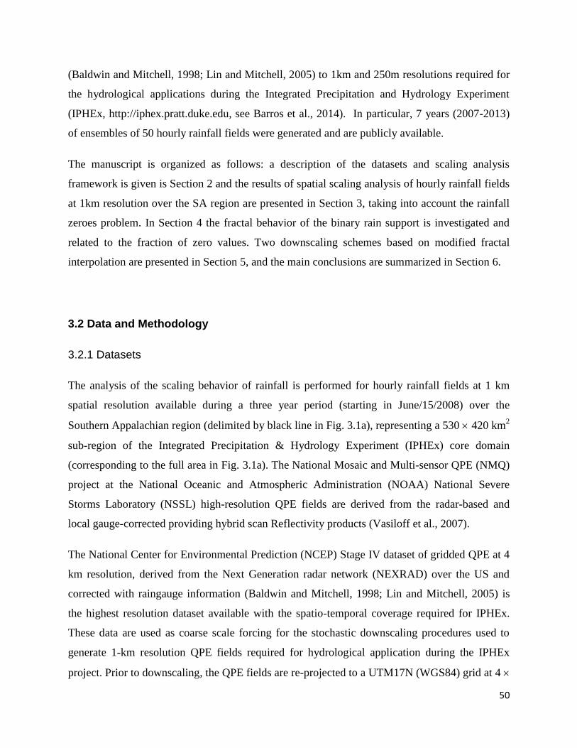
50
(Baldwin and Mitchell, 1998; Lin and Mitchell, 2005) to 1km and 250m resolutions required for
the hydrological applications during the Integrated Precipitation and Hydrology Experiment
(IPHEx, http://iphex.pratt.duke.edu, see Barros et al., 2014). In particular, 7 years (2007-2013)
of ensembles of 50 hourly rainfall fields were generated and are publicly available.
The manuscript is organized as follows: a description of the datasets and scaling analysis
framework is given is Section 2 and the results of spatial scaling analysis of hourly rainfall fields
at 1km resolution over the SA region are presented in Section 3, taking into account the rainfall
zeroes problem. In Section 4 the fractal behavior of the binary rain support is investigated and
related to the fraction of zero values. Two downscaling schemes based on modified fractal
interpolation are presented in Section 5, and the main conclusions are summarized in Section 6.
3.2 Data and Methodology
3.2.1 Datasets
The analysis of the scaling behavior of rainfall is performed for hourly rainfall fields at 1 km
spatial resolution available during a three year period (starting in June/15/2008) over the
Southern Appalachian region (delimited by black line in Fig. 3.1a), representing a 530 420 km2
sub-region of the Integrated Precipitation & Hydrology Experiment (IPHEx) core domain
(corresponding to the full area in Fig. 3.1a). The National Mosaic and Multi-sensor QPE (NMQ)
project at the National Oceanic and Atmospheric Administration (NOAA) National Severe
Storms Laboratory (NSSL) high-resolution QPE fields are derived from the radar-based and
local gauge-corrected providing hybrid scan Reflectivity products (Vasiloff et al., 2007).
The National Center for Environmental Prediction (NCEP) Stage IV dataset of gridded QPE at 4
km resolution, derived from the Next Generation radar network (NEXRAD) over the US and
corrected with raingauge information (Baldwin and Mitchell, 1998; Lin and Mitchell, 2005) is
the highest resolution dataset available with the spatio-temporal coverage required for IPHEx.
These data are used as coarse scale forcing for the stochastic downscaling procedures used to
generate 1-km resolution QPE fields required for hydrological application during the IPHEx
project. Prior to downscaling, the QPE fields are re-projected to a UTM17N (WGS84) grid at 4
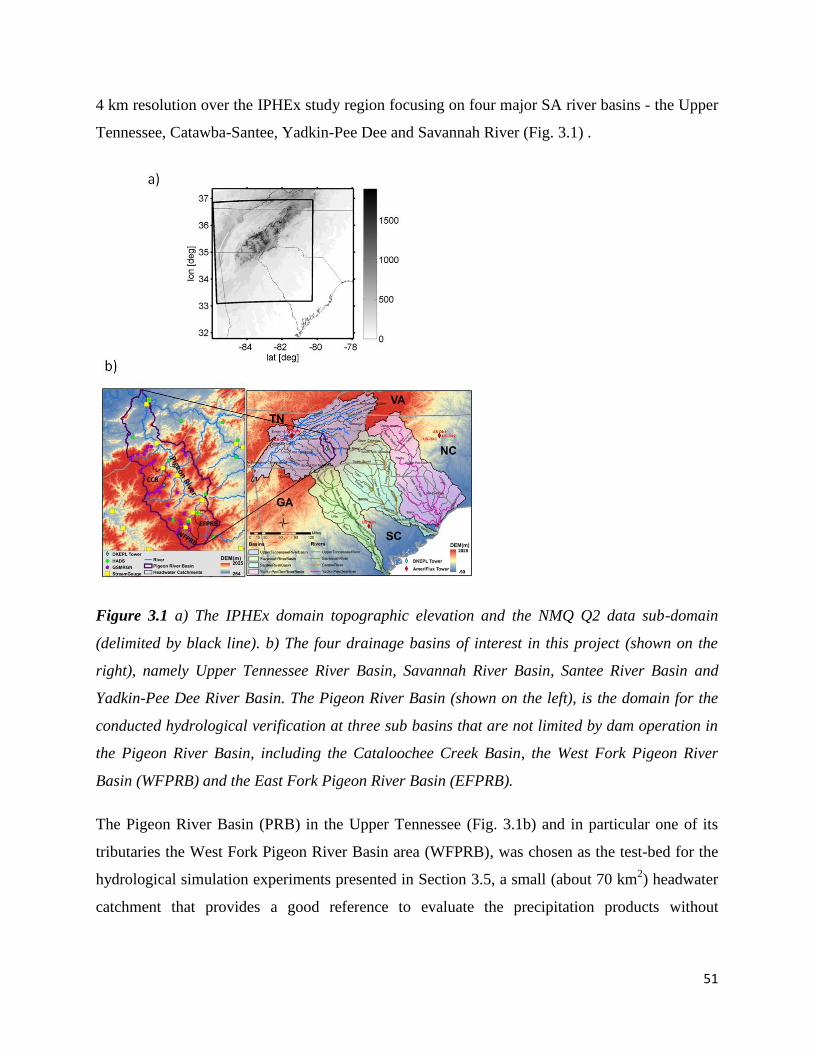
51
4 km resolution over the IPHEx study region focusing on four major SA river basins - the Upper
Tennessee, Catawba-Santee, Yadkin-Pee Dee and Savannah River (Fig. 3.1) .
Figure 3.1 a) The IPHEx domain topographic elevation and the NMQ Q2 data sub-domain
(delimited by black line). b) The four drainage basins of interest in this project (shown on the
right), namely Upper Tennessee River Basin, Savannah River Basin, Santee River Basin and
Yadkin-Pee Dee River Basin. The Pigeon River Basin (shown on the left), is the domain for the
conducted hydrological verification at three sub basins that are not limited by dam operation in
the Pigeon River Basin, including the Cataloochee Creek Basin, the West Fork Pigeon River
Basin (WFPRB) and the East Fork Pigeon River Basin (EFPRB).
The Pigeon River Basin (PRB) in the Upper Tennessee (Fig. 3.1b) and in particular one of its
tributaries the West Fork Pigeon River Basin area (WFPRB), was chosen as the test-bed for the
hydrological simulation experiments presented in Section 3.5, a small (about 70 km2) headwater
catchment that provides a good reference to evaluate the precipitation products without
52
introducing the spatial integration artifacts of the simulations at large scales. The hydrological
model and simulation setup were described in detail in Tao and Barros (2013, 2014a).
3.2.2 Scaling Analysis
Based on cascade phenomenology models, the spatial scaling behavior of statistical scale
invariant fields is often investigated by analyzing their statistical moments, which are expected to
obey the generic multiscaling relation (Lavallée et al., 1993):
(3.1)
where < > represents the statistical average, q is the moment order generalized to any positive
real number, is the scale ratio, L0 being the outer scale of the cascade (the largest scale
of variability) and l the scale of the observation, or simulation. Here, is a quantity that is on
average conserved from scale to scale, analogous to turbulent flux in cascade models. This
quantity is non-dimensionalized and normalized, such that . For a multifractal
quantity the moment scaling exponent function, K(q) is a convex nonlinear function of q and
thus infinite number of scaling exponents are necessary to fully characterize the scaling behavior.
Based on multiplicative cascade processes and the stability properties of cascade generators,
Schertzer and Lovejoy (1987) showed that K(q) can be modeled by Eq. 2 reducing the problem
to the determination of two parameters, and C1.
(3.2)
The Levy index, is defined in the interval [0,2] and indicates the degree of multifractality,
with for monofractals. The co-dimension of the mean singularity, C1, describes the
sparseness or non-homogeneity of the mean of the process such that the higher the C1 value the
more intermittent the field, with more sparse peaks of higher amplitude (Sun and Barros, 2010).
Because there is no physical basis to assume that rainfall fields should be conserved on a scale
by scale basis, and in fact most geophysical fields are found to behave as non-conservative
quantities, a third multifractal parameter must be introduced, the non-conservation parameter, H,
53
which represents the degree of smoothness of the process. In the canonical non-conservative
case, the mean exhibits scale dependence, , while for a conservative process (where
H=0) it is found that The non-conservation parameter can be easily estimated
from the slope of the log-log plot of the first order structure function against the lag (Harris et al.,
2001; Lovejoy et al., 2008):
(3.3)
where is a fluctuation in the field F over a distance l. When H is nonzero,
an additional fractional integration of order H is needed to obtain the fractionally integrated flux
(FIF), corresponding to the conserved quantity. However, in practice, taking normalized absolute
value of the finite difference gradient at the highest resolution available, l0, provides a good
approximation of the underlying conservative cascade (Lavallée et al., 1993):
(3.4)
The FIF estimates given by Eq. 3.4 are normalized and systematically degraded to lower
resolutions (lower values of ) by spatial averaging to obtain used to compute the statistical
moments in Eq. 3.1. Linear relations in log-log plots of the q-order moments against indicate
the presence of underlying multifractal behavior in the rainfall fields, the slopes being estimates
of K(q). The parameters and C1 can be estimated using the simple relationships (e.g. Lovejoy
et al., 2008; Verrier et al., 2010): and . Alternatively more
sophisticated methods such as the Double Trace Moment (DTM) technique described by
Lavallée et al. (1993) can be used to obtain estimates of the UM parameters.
Spectral analysis can also be used to investigate the presence of scale-invariant behavior over a
wide range of scales in rainfall fields. Spatial scaling invariance manifests itself as log-log
linearity of the power spectrum in space:
(3.5)
where represents the wavenumber in the direction. Consequently, the spectral exponent
that describes the variability of the rainfall field as a function of scale can be estimated using
least square regression in log-log plots.
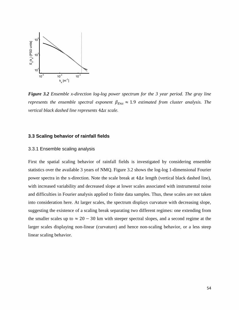
54
Figure 3.2 Ensemble x-direction log-log power spectrum for the 3 year period. The gray line
represents the ensemble spectral exponent estimated from cluster analysis. The
vertical black dashed line represents scale.
3.3 Scaling behavior of rainfall fields
3.3.1 Ensemble scaling analysis
First the spatial scaling behavior of rainfall fields is investigated by considering ensemble
statistics over the available 3 years of NMQ. Figure 3.2 shows the log-log 1-dimensional Fourier
power spectra in the x-direction. Note the scale break at length (vertical black dashed line),
with increased variability and decreased slope at lower scales associated with instrumental noise
and difficulties in Fourier analysis applied to finite data samples. Thus, these scales are not taken
into consideration here. At larger scales, the spectrum displays curvature with decreasing slope,
suggesting the existence of a scaling break separating two different regimes: one extending from
the smaller scales up to km with steeper spectral slopes, and a second regime at the
larger scales displaying non-linear (curvature) and hence non-scaling behavior, or a less steep
linear scaling behavior.
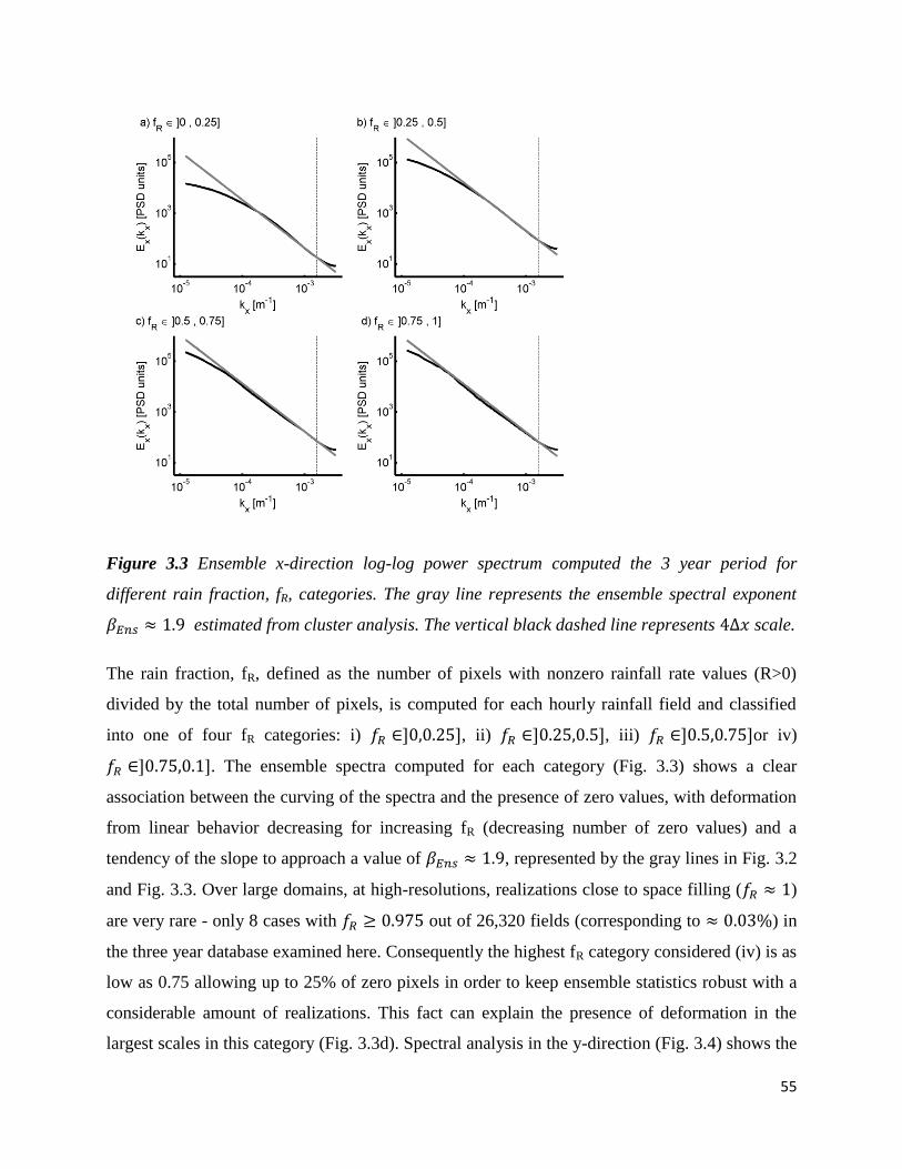
55
Figure 3.3 Ensemble x-direction log-log power spectrum computed the 3 year period for
different rain fraction, fR, categories. The gray line represents the ensemble spectral exponent
estimated from cluster analysis. The vertical black dashed line represents scale.
The rain fraction, fR, defined as the number of pixels with nonzero rainfall rate values (R>0)
divided by the total number of pixels, is computed for each hourly rainfall field and classified
into one of four fR categories: i) , ii) , iii) or iv)
. The ensemble spectra computed for each category (Fig. 3.3) shows a clear
association between the curving of the spectra and the presence of zero values, with deformation
from linear behavior decreasing for increasing fR (decreasing number of zero values) and a
tendency of the slope to approach a value of , represented by the gray lines in Fig. 3.2
and Fig. 3.3. Over large domains, at high-resolutions, realizations close to space filling ( )
are very rare - only 8 cases with out of 26,320 fields (corresponding to ) in
the three year database examined here. Consequently the highest fR category considered (iv) is as
low as 0.75 allowing up to 25% of zero pixels in order to keep ensemble statistics robust with a
considerable amount of realizations. This fact can explain the presence of deformation in the
largest scales in this category (Fig. 3.3d). Spectral analysis in the y-direction (Fig. 3.4) shows the

56
same decreasing curvature and tendency to as fR increases, providing further
robustness to the results.
Figure 3.4 Same as Fig. 3.3 but in the y-direction.
Using the same fR classification, similar deformation associated with the presence of zero values
is found for the ensemble first order structure function (Fig. 3.5), with more pronounced
curvature at the larger scales for decreasing fR and associated decreasing slope. As fR increases
there is a tendency towards an ensemble linear scaling behavior, characterized by .
The scales smaller than are not considered for the same reasons enunciated for the spectral
analysis. Figure 3.6 shows the log-log plots of ensemble x-direction statistical moments against
the scale ratio, (see Eq. 3.1). The statistical moments, Mq, were computed for different fR
categories and different moment orders q (from bottom q=0.5 at 0.5 steps to q=2.5 at the top). As
commonly reported in the relevant literature for spatial scaling analysis, we restrict our study to
orders only up to q=2.5 due to sample size limitations and divergence of moments at orders
greater than critical order (e.g. Lovejoy et al., 2008; Nykanen, 2008). Consistent with the
results of spectral and structure function analysis, Mq also shows curvature and break of the

57
scaling behavior at the large scales (small ) for low fR cases, but approaches linear scaling
behavior as fR increases. The gray lines in Fig. 6 are obtained by linear fit between and the
domain length scale, and the slopes are estimates for the moment scaling function exponent K(q).
As fR increases, increases approaching 1.8 while C1 decreases approaching 0.1. These hold for
the ensemble structure function and moment scaling analysis in the y-direction with similar
scaling parameters (not shown).
Figure 3.5 Log-log plot of the first order structure function, S1, against the scale lag, for
different fR categories. Gray dashed lines represent fitted ensemble slopes obtained from high fR
cases, corresponding to .
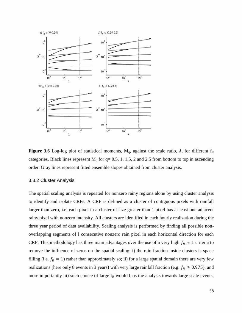
58
Figure 3.6 Log-log plot of statistical moments, Mq, against the scale ratio, , for different fR
categories. Black lines represent Mq for q= 0.5, 1, 1.5, 2 and 2.5 from bottom to top in ascending
order. Gray lines represent fitted ensemble slopes obtained from cluster analysis.
3.3.2 Cluster Analysis
The spatial scaling analysis is repeated for nonzero rainy regions alone by using cluster analysis
to identify and isolate CRFs. A CRF is defined as a cluster of contiguous pixels with rainfall
larger than zero, i.e. each pixel in a cluster of size greater than 1 pixel has at least one adjacent
rainy pixel with nonzero intensity. All clusters are identified in each hourly realization during the
three year period of data availability. Scaling analysis is performed by finding all possible non-
overlapping segments of l consecutive nonzero rain pixel in each horizontal direction for each
CRF. This methodology has three main advantages over the use of a very high criteria to
remove the influence of zeros on the spatial scaling: i) the rain fraction inside clusters is space
filling (i.e. ) rather than approximately so; ii) for a large spatial domain there are very few
realizations (here only 8 events in 3 years) with very large rainfall fraction (e.g. ); and
more importantly iii) such choice of large fR would bias the analysis towards large scale events,

59
such as large mesoscale convective systems (MCS) or large synoptic-systems. Consequently, the
scaling behavior would not capture the scaling behavior of smaller structures such as summer
and/or orographic convective events, which are critical to this region. The ensemble Fourier 1-
directional spectra is computed over all segments from all CRFs in the dataset. The analysis is
performed for segment length, l, values of l=64 and l=128 pixels. The results show strong scaling
(Fig. 3.7), extending from 4 to 128 km with consistent average slopes . The curvature
problems in scaling remain at small scales (below about ) for the same reasons explained
above.
Figure 3.7 Ensemble x-direction log-log power spectrum for the 3 year period computed inside
rain clusters only, for segment lengths a) l=64 km and b) l=128km and corresponding least-
square fit (gray). The vertical black dashed line represents scale.
Ensemble moment scaling analysis from rain cluster segments with l=64 and 128 km, also show
remarkable scaling with and for both segment lengths (Fig. 3.8), remarkably
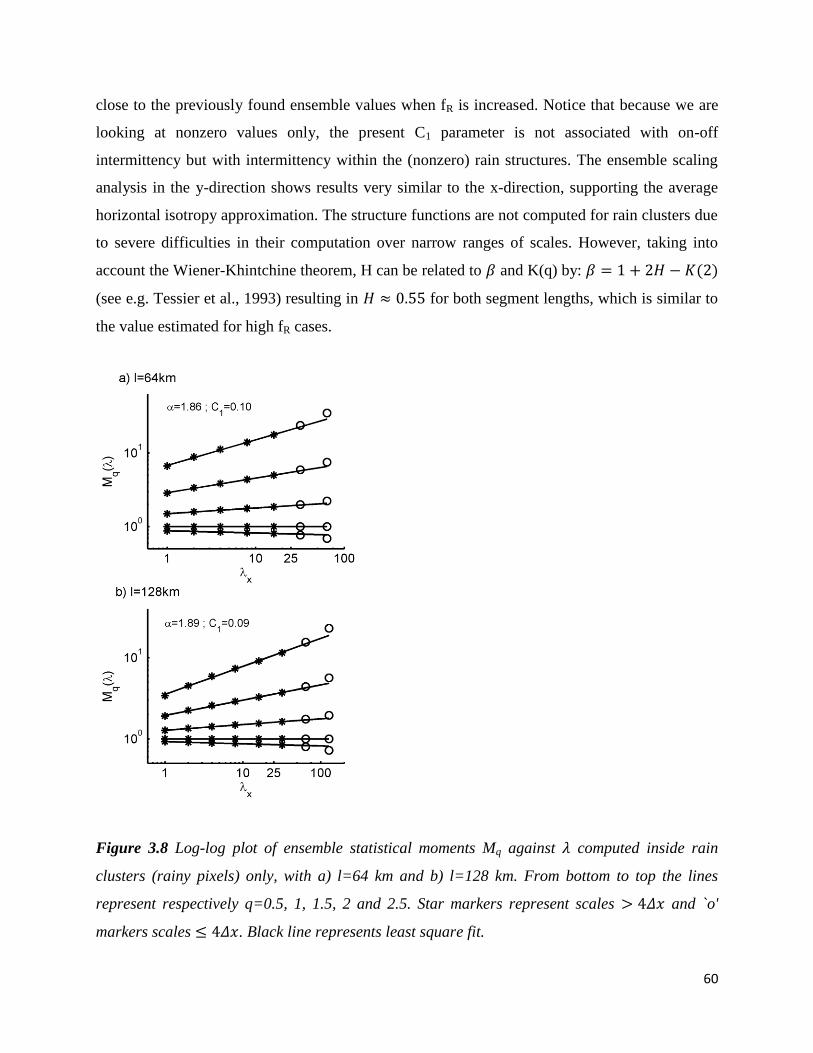
60
close to the previously found ensemble values when fR is increased. Notice that because we are
looking at nonzero values only, the present C1 parameter is not associated with on-off
intermittency but with intermittency within the (nonzero) rain structures. The ensemble scaling
analysis in the y-direction shows results very similar to the x-direction, supporting the average
horizontal isotropy approximation. The structure functions are not computed for rain clusters due
to severe difficulties in their computation over narrow ranges of scales. However, taking into
account the Wiener-Khintchine theorem, H can be related to and K(q) by:
(see e.g. Tessier et al., 1993) resulting in for both segment lengths, which is similar to
the value estimated for high fR cases.
Figure 3.8 Log-log plot of ensemble statistical moments Mq against computed inside rain
clusters (rainy pixels) only, with a) l=64 km and b) l=128 km. From bottom to top the lines
represent respectively q=0.5, 1, 1.5, 2 and 2.5. Star markers represent scales and `o'
markers scales . Black line represents least square fit.
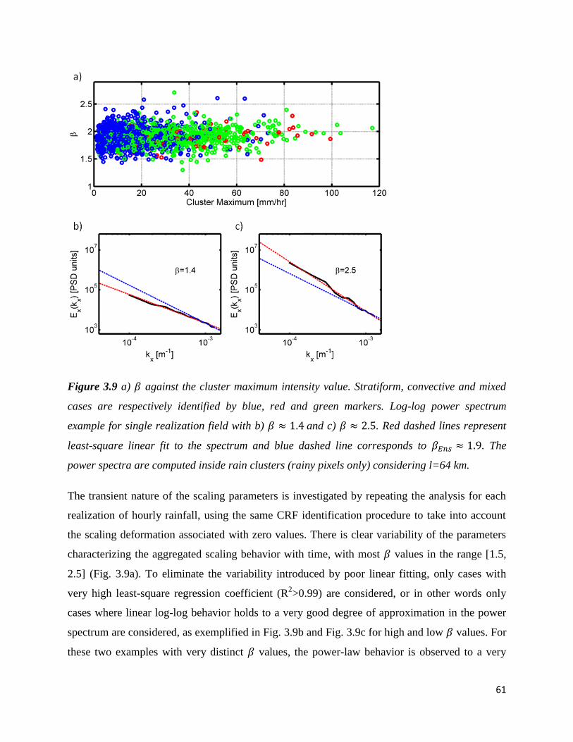
61
Figure 3.9 a) against the cluster maximum intensity value. Stratiform, convective and mixed
cases are respectively identified by blue, red and green markers. Log-log power spectrum
example for single realization field with b) and c) . Red dashed lines represent
least-square linear fit to the spectrum and blue dashed line corresponds to . The
power spectra are computed inside rain clusters (rainy pixels only) considering l=64 km.
The transient nature of the scaling parameters is investigated by repeating the analysis for each
realization of hourly rainfall, using the same CRF identification procedure to take into account
the scaling deformation associated with zero values. There is clear variability of the parameters
characterizing the aggregated scaling behavior with time, with most values in the range [1.5,
2.5] (Fig. 3.9a). To eliminate the variability introduced by poor linear fitting, only cases with
very high least-square regression coefficient (R2>0.99) are considered, or in other words only
cases where linear log-log behavior holds to a very good degree of approximation in the power
spectrum are considered, as exemplified in Fig. 3.9b and Fig. 3.9c for high and low values. For
these two examples with very distinct values, the power-law behavior is observed to a very
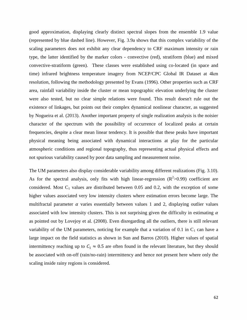
62
good approximation, displaying clearly distinct spectral slopes from the ensemble 1.9 value
(represented by blue dashed line). However, Fig. 3.9a shows that this complex variability of the
scaling parameters does not exhibit any clear dependency to CRF maximum intensity or rain
type, the latter identified by the marker colors - convective (red), stratiform (blue) and mixed
convective-stratiform (green). These classes were established using co-located (in space and
time) infrared brightness temperature imagery from NCEP/CPC Global IR Dataset at 4km
resolution, following the methodology presented by Evans (1996). Other properties such as CRF
area, rainfall variability inside the cluster or mean topographic elevation underlying the cluster
were also tested, but no clear simple relations were found. This result doesn't rule out the
existence of linkages, but points out their complex dynamical nonlinear character, as suggested
by Nogueira et al. (2013). Another important property of single realization analysis is the noisier
character of the spectrum with the possibility of occurrence of localized peaks at certain
frequencies, despite a clear mean linear tendency. It is possible that these peaks have important
physical meaning being associated with dynamical interactions at play for the particular
atmospheric conditions and regional topography, thus representing actual physical effects and
not spurious variability caused by poor data sampling and measurement noise.
The UM parameters also display considerable variability among different realizations (Fig. 3.10).
As for the spectral analysis, only fits with high linear-regression (R2>0.99) coefficient are
considered. Most C1 values are distributed between 0.05 and 0.2, with the exception of some
higher values associated very low intensity clusters where estimation errors become large. The
multifractal parameter varies essentially between values 1 and 2, displaying outlier values
associated with low intensity clusters. This is not surprising given the difficulty in estimating
as pointed out by Lovejoy et al. (2008). Even disregarding all the outliers, there is still relevant
variability of the UM parameters, noticing for example that a variation of 0.1 in C1 can have a
large impact on the field statistics as shown in Sun and Barros (2010). Higher values of spatial
intermittency reaching up to are often found in the relevant literature, but they should
be associated with on-off (rain/no-rain) intermittency and hence not present here where only the
scaling inside rainy regions is considered.
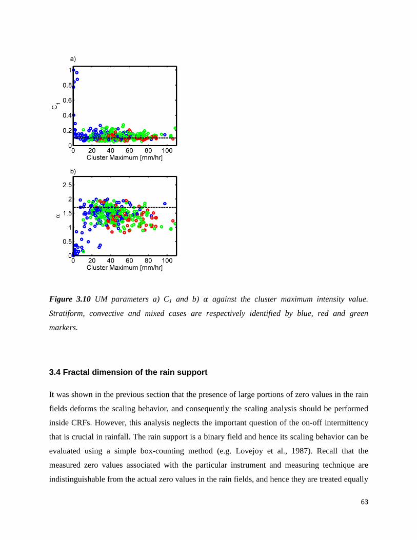
63
Figure 3.10 UM parameters a) C1 and b) against the cluster maximum intensity value.
Stratiform, convective and mixed cases are respectively identified by blue, red and green
markers.
3.4 Fractal dimension of the rain support
It was shown in the previous section that the presence of large portions of zero values in the rain
fields deforms the scaling behavior, and consequently the scaling analysis should be performed
inside CRFs. However, this analysis neglects the important question of the on-off intermittency
that is crucial in rainfall. The rain support is a binary field and hence its scaling behavior can be
evaluated using a simple box-counting method (e.g. Lovejoy et al., 1987). Recall that the
measured zero values associated with the particular instrument and measuring technique are
indistinguishable from the actual zero values in the rain fields, and hence they are treated equally

64
as field zeroes. For any given object embedded in a D-dimensional Euclidean domain of size LD,
the number of D-dimensional boxes of size lD required to cover the object can be expressed as:
(3.6)
where Df is the fractal dimension of the object and cL is an adimensional coefficient which
depends on L and the shape of the object. Here we focus on the 2-dimensional embedding space
case, D=2, but the results can be easily generalized to other dimensions. The area, A, of the
structure can be estimated from the associated with l2 sized boxes:
(3.7)
When the object is itself 2-dimensional, then Df=2 and the expression reduces to
. It can be shown that this expression is valid for the usual (nonfractal) 2-dimensional
shapes or linear compositions of them, as long as cL is chosen appropriately depending on the
size of the embedding space L and the geometrical shape‡. However, when the dimension of the
object is a non-integer value (1<Df <2) the area will depend on the measurement resolution. For
a single scaling field the parameters Df and cL are constant with scale and consequently better
suited to characterize the object geometry. These parameters can be estimated from the slope of
the log-log plot of against :
(3.8)
The rain fraction at resolution is the number of boxes necessary to cover the rain support
divided by the total number of boxes in the domain (
) and can be related to Df by:
(3.9)
which can be re-written as:
‡ For example for a square of side s we have cL=[s/L]
2, which in the particular case s=L becomes cL =1. If L is the side
of the smallest bounding box for a triangle or a circle, then cL is respectively 1/2 or . For larger L values, cL will be proportionally smaller.

65
(3.10)
Figure 3.11 a) Fractal dimension Df and b) cL of the rain support against the respective rain
fraction fR. Markers represent empirical estimates using box-counting methods and black line
represents theoretical values obtained from Eq. 3.10 assuming cL=1. Stratiform, convective and
mixed cases are respectively identified by blue, red and green markers.
This implies that fR computed at a certain resolution will be a function of Df and cL.
Consequently, for a rainfall field measurement at a particular resolution in a particular domain,
there will be a corresponding value of Df, which will be a good estimate as long as . This
is illustrated in Fig. 3.11a that shows the estimated Df values for each realization against the
respective fR at 1 km resolution. Red markers represent convective cases, blue represent
stratiform, and green represent mixed cases, all falling under the same dependency curve. Fig.
3.11b shows the estimated cL values for each realization against the respective fR at 1 km
resolution. For higher fR values, i.e. domain filling rain supports, there is an expected tendency of
and , while for low fR there is more variability in cL. Recall that fractal
constructions that are built starting from a space filling line, square or cube, such as the Cantor
66
set, the Sierpinsky carpet or the Menger sponge have cL equal to unity§. Assuming that the
support of surface rainfall is built by transformations (including thresholding) of space filling
fields such as atmospheric water vapor, temperature and wind (although it has non-space-filling
fields at intermediate steps, such as cloud water and rain water) one can hypothesize that for
surface rainfall fields cL=1. This hypothesis is grounded in the behavior illustrated by the thick
black dashed line in Fig. 3.11a computed from Eq. 3.10 with cL=1, that displays a very close fit
to the empirically computed fractal dimensions. Hence, the large variability in cL values can be
attributed to estimation difficulties for small nonzero data amounts far from the limit. In
summary, the rain support is itself fractal with a Df value that depends on the concurrent
atmospheric conditions and forcing. Theoretical a priori determination of Df for particular
atmospheric conditions and forcings has not been obtained yet.
3.5 Spatial downscaling
The fact that stochastic scale invariant behavior is a good approximation even when single
realizations are considered makes it a very attractive and promising tool for constraining
downscaling and sub-grid parameterization applications. In this section, we leverage this
tendency to perform spatial downscaling of seven years of hourly Stage IV rainfall fields from
their original 4 km resolution to the 1 km resolution grid of IPHEx. Based on previous works of
Bindlish and Barros (1996) this can be achieved by generating a modified fractal Brownian
surface (fBs) with the desired fine resolution, number of grid points and correct spectral
exponent and use it as an interpolation surface. This methodology preserves the known coarse
resolution portion of the power spectrum, extrapolating it to sub-grid scale wavenumbers using
the correct spectral slope and amplitude. Thus, one can obtain a higher-resolution downscaled
version of the field that preserves the spatial structure and correct scale invariant behavior, with
coherent variability at the fine scales as schematically illustrated in Fig. 3.12. The preservation of
the exact coarse resolution information can be obtained by normalizing the fBs by a coarse
resolution version of itself at the same resolution as the original coarse data (see Rebora et al.,
§ The Cantor set starts from a 1-dimensional space-filling line and has [ ], the Sierpinsky carpet
starts from a space-filling square and has [ ], and the Menger Sponge starts from a space-filling
cube and has [ ].
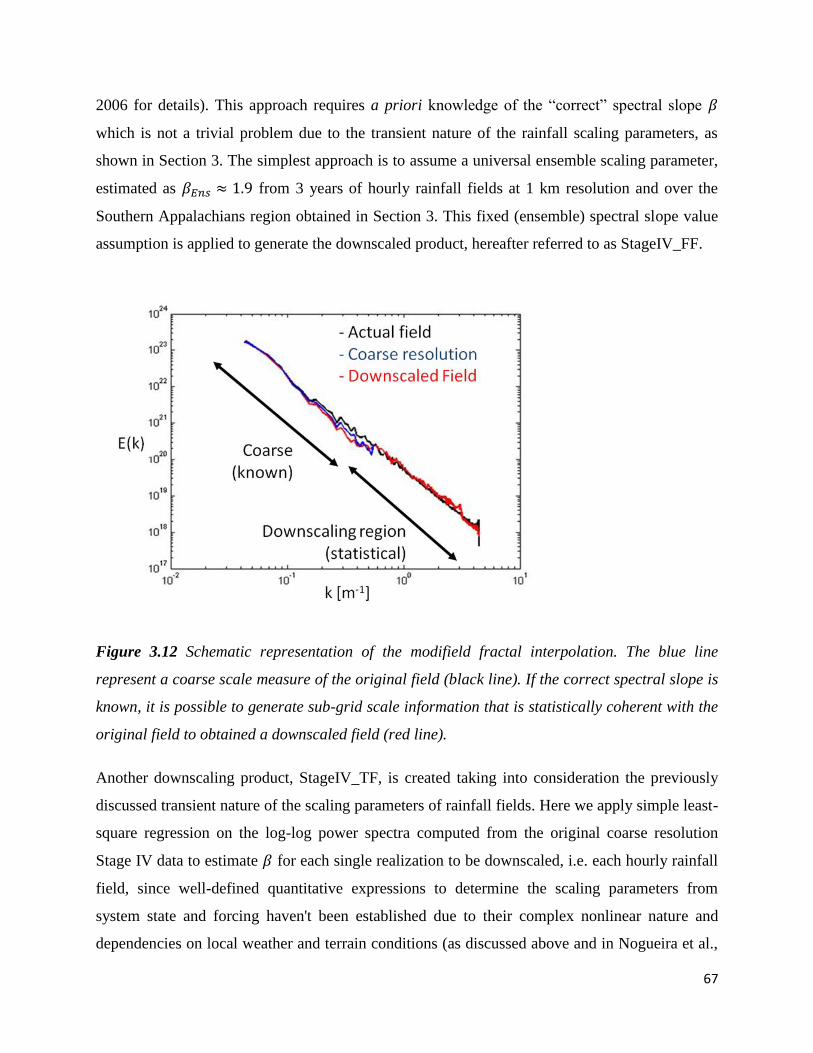
67
2006 for details). This approach requires a priori knowledge of the “correct” spectral slope
which is not a trivial problem due to the transient nature of the rainfall scaling parameters, as
shown in Section 3. The simplest approach is to assume a universal ensemble scaling parameter,
estimated as from 3 years of hourly rainfall fields at 1 km resolution and over the
Southern Appalachians region obtained in Section 3. This fixed (ensemble) spectral slope value
assumption is applied to generate the downscaled product, hereafter referred to as StageIV_FF.
Figure 3.12 Schematic representation of the modifield fractal interpolation. The blue line
represent a coarse scale measure of the original field (black line). If the correct spectral slope is
known, it is possible to generate sub-grid scale information that is statistically coherent with the
original field to obtained a downscaled field (red line).
Another downscaling product, StageIV_TF, is created taking into consideration the previously
discussed transient nature of the scaling parameters of rainfall fields. Here we apply simple least-
square regression on the log-log power spectra computed from the original coarse resolution
Stage IV data to estimate for each single realization to be downscaled, i.e. each hourly rainfall
field, since well-defined quantitative expressions to determine the scaling parameters from
system state and forcing haven't been established due to their complex nonlinear nature and
dependencies on local weather and terrain conditions (as discussed above and in Nogueira et al.,
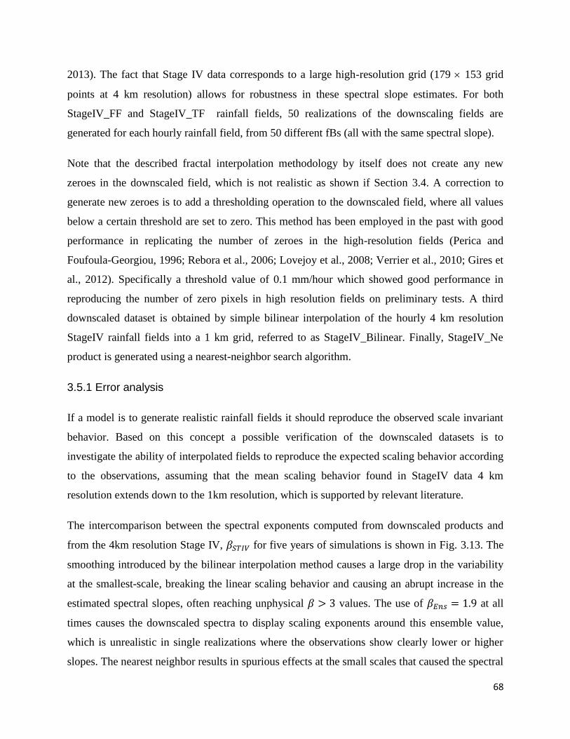
68
2013). The fact that Stage IV data corresponds to a large high-resolution grid (179 153 grid
points at 4 km resolution) allows for robustness in these spectral slope estimates. For both
StageIV_FF and StageIV_TF rainfall fields, 50 realizations of the downscaling fields are
generated for each hourly rainfall field, from 50 different fBs (all with the same spectral slope).
Note that the described fractal interpolation methodology by itself does not create any new
zeroes in the downscaled field, which is not realistic as shown if Section 3.4. A correction to
generate new zeroes is to add a thresholding operation to the downscaled field, where all values
below a certain threshold are set to zero. This method has been employed in the past with good
performance in replicating the number of zeroes in the high-resolution fields (Perica and
Foufoula-Georgiou, 1996; Rebora et al., 2006; Lovejoy et al., 2008; Verrier et al., 2010; Gires et
al., 2012). Specifically a threshold value of 0.1 mm/hour which showed good performance in
reproducing the number of zero pixels in high resolution fields on preliminary tests. A third
downscaled dataset is obtained by simple bilinear interpolation of the hourly 4 km resolution
StageIV rainfall fields into a 1 km grid, referred to as StageIV_Bilinear. Finally, StageIV_Ne
product is generated using a nearest-neighbor search algorithm.
3.5.1 Error analysis
If a model is to generate realistic rainfall fields it should reproduce the observed scale invariant
behavior. Based on this concept a possible verification of the downscaled datasets is to
investigate the ability of interpolated fields to reproduce the expected scaling behavior according
to the observations, assuming that the mean scaling behavior found in StageIV data 4 km
resolution extends down to the 1km resolution, which is supported by relevant literature.
The intercomparison between the spectral exponents computed from downscaled products and
from the 4km resolution Stage IV, for five years of simulations is shown in Fig. 3.13. The
smoothing introduced by the bilinear interpolation method causes a large drop in the variability
at the smallest-scale, breaking the linear scaling behavior and causing an abrupt increase in the
estimated spectral slopes, often reaching unphysical values. The use of at all
times causes the downscaled spectra to display scaling exponents around this ensemble value,
which is unrealistic in single realizations where the observations show clearly lower or higher
slopes. The nearest neighbor results in spurious effects at the small scales that caused the spectral
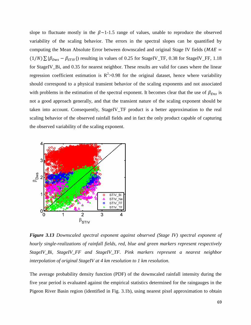
69
slope to fluctuate mostly in the 1-1.5 range of values, unable to reproduce the observed
variability of the scaling behavior. The errors in the spectral slopes can be quantified by
computing the Mean Absolute Error between downscaled and original Stage IV fields (
) resulting in values of 0.25 for StageIV_TF, 0.38 for StageIV_FF, 1.18
for StageIV_Bi, and 0.35 for nearest neighbor. These results are valid for cases where the linear
regression coefficient estimation is R2>0.98 for the original dataset, hence where variability
should correspond to a physical transient behavior of the scaling exponents and not associated
with problems in the estimation of the spectral exponent. It becomes clear that the use of is
not a good approach generally, and that the transient nature of the scaling exponent should be
taken into account. Consequently, StageIV_TF product is a better approximation to the real
scaling behavior of the observed rainfall fields and in fact the only product capable of capturing
the observed variability of the scaling exponent.
Figure 3.13 Downscaled spectral exponent against observed (Stage IV) spectral exponent of
hourly single-realizations of rainfall fields, red, blue and green markers represent respectively
StageIV_Bi, StageIV_FF and StageIV_TF. Pink markers represent a nearest neighbor
interpolation of original StageIV at 4 km resolution to 1 km resolution.
The average probability density function (PDF) of the downscaled rainfall intensity during the
five year period is evaluated against the empirical statistics determined for the raingauges in the
Pigeon River Basin region (identified in Fig. 3.1b), using nearest pixel approximation to obtain
70
point values over the raingauge locations. All downscaling products show clear underestimation
of the low intensity (< 5 mm/hr) precipitation frequency (Fig. 3.14) due to limitations in the
algorithms used to estimate rainfall from radar measurements for StageIV products. Note that
this is likely to cause problems for water budget studies as light rainfall represents a substantial
part of the water cycle (Wilson and Barros, 2014). For intermediate intensities, all products show
good reproduction of the raingauge observations, particularly considering that comparison is
between point measurements and 1km resolution gridded data. The point-to-pixel scale gap
should also be responsible for the general PDF underestimation at the highest intensities for all
gridded products. Bilinear interpolation causes the largest underestimation as expected by its
smoother character. Also, the smoothing introduced by the ensemble averaging operations in
StageIV_FF and StageIV_TF products introduces a frequency decrease at the highest intensities,
as it can be seen by comparing the results against a randomly chosen single realization out of the
50 realizations available at each time step (light blue and pink lines). The results for StageIV_TF
show a slightly better ability to represent the probabilities of high intensity rainfall values than
StageIV_FF, providing further support for the transient character of the scaling behavior.
Figure 3.14 Intercomparison of probability density function (PDF) over the PRB raingauges
(identified in Fig. 1) point locations during the five year period. Black line is computed from
local raingauge data and the other lines corresponded to 1km resolution downscaled products.
StageIV_FF_SR (light blue) and StageIV_TF_SR (pink) represent the statistics for a randomly
chosen single realization (out of the 50 available) at each time instant. For 1km downscaled
products nearest pixel approximation is used to obtain point values over the raingauge locations.
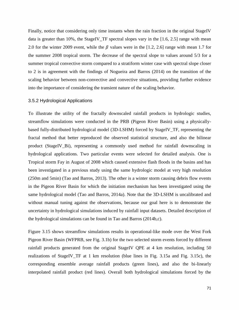
71
Finally, notice that considering only time instants when the rain fraction in the original StageIV
data is greater than 10%, the StageIV_TF spectral slopes vary in the [1.6, 2.5] range with mean
2.0 for the winter 2009 event, while the values were in the [1.2, 2.6] range with mean 1.7 for
the summer 2008 tropical storm. The decrease of the spectral slope to values around 5/3 for a
summer tropical convective storm compared to a stratiform winter case with spectral slope closer
to 2 is in agreement with the findings of Nogueira and Barros (2014) on the transition of the
scaling behavior between non-convective and convective situations, providing further evidence
into the importance of considering the transient nature of the scaling behavior.
3.5.2 Hydrological Applications
To illustrate the utility of the fractally downscaled rainfall products in hydrologic studies,
streamflow simulations were conducted in the PRB (Pigeon River Basin) using a physically-
based fully-distributed hydrological model (3D-LSHM) forced by StageIV_TF, representing the
fractal method that better reproduced the observed statistical structure, and also the bilinear
product (StageIV_Bi), representing a commonly used method for rainfall downscaling in
hydrological applications. Two particular events were selected for detailed analysis. One is
Tropical storm Fay in August of 2008 which caused extensive flash floods in the basins and has
been investigated in a previous study using the same hydrologic model at very high resolution
(250m and 5min) (Tao and Barros, 2013). The other is a winter storm causing debris flow events
in the Pigeon River Basin for which the initiation mechanism has been investigated using the
same hydrological model (Tao and Barros, 2014a). Note that the 3D-LSHM is uncalibrated and
without manual tuning against the observations, because our goal here is to demonstrate the
uncertainty in hydrological simulations induced by rainfall input datasets. Detailed description of
the hydrological simulations can be found in Tao and Barros (2014b,c).
Figure 3.15 shows streamflow simulations results in operational-like mode over the West Fork
Pigeon River Basin (WFPRB, see Fig. 3.1b) for the two selected storm events forced by different
rainfall products generated from the original StageIV QPE at 4 km resolution, including 50
realizations of StageIV_TF at 1 km resolution (blue lines in Fig. 3.15a and Fig. 3.15c), the
corresponding ensemble average rainfall products (green lines), and also the bi-linearly
interpolated rainfall product (red lines). Overall both hydrological simulations forced by the

72
fractally downscaled products exhibit good skill against the observed hydrograph (black lines in
Fig. 15) especially with regard to the timing and magnitude of peak discharge. The performance
of the fractal downscaled products quantified using the Nash-Sutcliffe efficiency (NSE) of the
streamflow for both events is summarized in Table 3.1. The NSE scores are high for all
simulations and substantially higher (closer to 1) for StageIV_TF, indicating better predictive
power consistent with expectations based on the error analysis results in the previous section. For
the winter storm case the fractal downscaling results in NSEs very close to unity with well
captured time-to-peak and peak flow values of the hydrographs (Fig. 3.15c). For the Tropical
Storm event (Fig. 15a), while the timing and shape of the stream flow peak are well reproduced
by both fractal downscaling methods, the ensemble products underestimate peak intensity and
overestimate the streamflow recession, explaining the decrease in NSE. The lack of skill in
reproducing the falling limb of the observed hydrograph may be associated with the specified
soil moisture and water table initial conditions and, or the uncalibrated parameters in the
hydrological model, and not with the rainfall forcing per se (see discussion by Tao and Barros
2013, 2014a).
Simulation Period Basins Rainfall dataset NSE
Aug. 25 – 28, 2008 WFPRB
StageIV_Bi 0.65
StageIV_TF 0.77
Jan. 5 – 10, 2009 WFPRB
StageIV_Bi 0.78
StageIV_TF 0.89
Table 3.1. Summary of NSE for hydrological simulations.
For the small resolution gain (4:1) between the original 4-km resolution and the IPHEx grid 1-
km resolution, the resulting spread in the simulated streamflow ensemble is narrow (blue lines in
Fig. 15a and Fig. 15c). Nonetheless the obtained variability is important since the single
realization solutions are able to attain higher streamflow peaks, closer to the observations, due to
the absence of the additional smoothing caused by ensemble averaging. The span of solutions
does in fact extend closer to the streamflow peak in the 2008 summer storm than when the

73
ensemble product is used. A larger spread of hydrograph solutions was obtained when a larger
resolution gain (16:1) was achieved by downscaling StageIV QPE from 4-km to 250m grid
spacing (Fig. 15b and Fig. 15d). At this finer resolution, the observed streamflow peak is always
within the 50 possible solutions obtained using both fractal products, while using the ensemble
rainfall products results in underestimation of the streamflow peak for both winter and summer
storms.
Figure 3.15 Examples of streamflow simulation in the WFPRB forced by StageIV_TF at 1km
resolution data for a) summer event (Tropical Storm Fay) in 2008 and b) winter storm in 2009,
and forced by StageIV_TF at 250 m resolution for c) summer event (Tropical Storm Fay) in 2008
and d) winter storm in 2009. Black lines represent observed streamflow. Blue lines represent the
span of plausible solutions generated by using each single member of the ensemble of fractally
downscaled fields as rainfall forcing. Green lines represent solutions of simulations forced by
the ensemble averaged rainfall field generated by fractal method. Redlines represent the solution
forced by bilinear interpolated rainfall fields.
74
Further evidence to the advantages of the fractal downscaling method presented here can be
found in Tao and Barros (2014b and 2014c) who used StageIV_FF and StageIV_TF 1 km
resolution products to force a 5-year (2007-2011) continuous simulation using the same
uncalibrated hydrologic model over the PRB, with significant overall increase of the NSE for all
types of rainfall events and various basins when fractal methods are used compared to bilinear
and nearest neighbor interpolation. Additionally, the performance for the fractal downscaling
results here is similar to results reported by Tao and Barros (2013, 2014a) using a locally
optimized precipitation product by merging observations from a dense raingauge network, which
is not included in the Stage IV products. This further gives credence to the robustness of the
fractal interpolation methods.
3.6 Conclusions
Radar derived QPE fields display spatial stochastic (multifractal) scale-invariance over a wide
range of scales (from km up to 100’s km). However, this scaling behavior is deformed by
the presence of large fractions of zero rain values, causing breaks and curvature to the log-log
linear spectral relations. One way to account for this deformation is to consider only rainfall
fields with high fR (low zero fractions). When the domains have large spatial extent, such as the
IPHEx domain over the SE US considered here, choosing only high fR cases can bias the analysis
towards large MCSs and synoptic-scale systems, potentially neglecting more localized
precipitation features such as summertime orographic convection. An alternative method is
presented here that relies on a spatial cluster identification algorithm to isolate (nonzero) CRFs,
inside which the spatial scaling behavior displays remarkable multifractal behavior, with
ensemble scaling parameters and , similar to the asymptotic
parameters found here when , also reported by Verrier et al. (2010).
When scaling analysis is performed on single realizations of hourly rainfall fields, the results
show important deviations from the ensemble scaling behavior, with values varying essentially
in the [1.5, 2.5] range. This implies that the multifractal properties of rainfall fields are transient
properties with variability that cannot be attributed to spurious effects associated with small
nonzero data samples or zero, and deformation of the scaling by the presence of large portions of
75
zero rainfall values. Instead, there is a complex nonlinear interdependence on the particular
atmospheric conditions and terrain forcing as argued by Barros et al. (2004), and in agreement
with the conclusions of Nogueira et al. (2013). It is also important to note that this type of
analysis on rain clusters circumvents the on-off intermittency in rainfall fields. Interestingly, it is
shown that the binary rain support is itself fractal, with fractal dimension that is by definition
tightly related to the fraction of rainy pixels, fR.
The scaling behavior of rainfall fields is a promising path for stochastic downscaling required to
bridge the gap between observed and simulated rainfall and the high-resolution requirements of
many hydrometeorological applications. Here, this approach was investigated by downscaling 7
years of hourly Stage IV rainfall fields at 4 km resolution to the 1km resolution IPHEx grid using
fractal interpolation methods in the Fourier domain. Two types of downscaled fractal products
were generated: one considering a fixed value of the scaling exponent estimated from the
ensemble analysis (StageIV_FF), and a second using a transient spectral exponent estimated
from each coarse resolution realization of the rainfall field (StageIV_TF). Both methodologies
are able to rapidly generate large ensembles of high resolution statistically robust fields without
any additional data or calibration requirements, conserving the coarse resolution information and
generating coherent small-scale variability and statistics, hence adding value to the original field.
It is important to note that the cross-scale conservation of the original statistical structure from
the coarse resolution information implies that the errors in these forcing datasets are propagated
into the downscaled fields, such as the tendency of the radar derived StageIV QPE to
underestimate low intensity rainfall or NWP (Numerical Weather Prediction) forecast errors for
example. Such issues should be resolved prior to downscaling and not by the downscaling
methodology itself.
The downscaled fields using transient estimation of the spectral scaling exponent result in better
coherence between the subgrid scale statistical structure and the respective coarse resolution
information when the scaling deviates significantly from behavior. Additionally,
StageIV_TF captures the high intensity rainfall statistics more accurately than StageIV_FF,
providing further support to the transient nature of the scaling behavior. Consequently
StageIV_TF was chosen as representing the best fractal downscaling method and used to force
hydrological simulations over the Pigeon River Basin in the Southern Appalachians. The
76
hydrological simulations forced by the 1 km resolution ensemble averaged fractal downscaled
fields overperformed the commonly used bilinear interpolation as expected. Non-fractal
interpolation methods are unable to reproduce the subgrid-scale variability resulting in
significant shortcoming in predicting extreme rainfall events associated with localized features,
though the specific impact on skill metrics will necessarily depend on basin scale and
geomorphic properties as well as the storm system proper. The results also show that the smooth
character of the ensemble downscaled rainfall products resulting from averaging over several
realizations cause an underestimation of the peak streamflow, particularly relevant for flashflood
causing events extreme rainfall events such as the 2008 summer Tropical storm Fay case studied
here. A more informative stochastic streamflow prediction was obtained by considering all the
hydrological simulations forced by each of 50 single realizations of the fractal downscaled
rainfall, that is an ensemble of hydrological simulations. The resulting spread of solutions was
better capable of capturing the observed intense streamflow peaks. Further improvement to the
streamflow solution spread was obtained by increasing the downscaling resolution to 250 m,
clearly demonstrating the high-resolution requirements of hydrological applications and the
utility of fractal downscaling to meet these requirements. At 250 m resolution the observed
streamflow associated with both storms was captured by the 50 member ensemble of stochastic
streamflow forecasts generated from StageIV_TF. Note that the generation of ensembles is
computationally inexpensive and does not require human interference or judgment and the fractal
downscaling can be ran fully automatically. The applications reported here and elsewhere (Tao
and Barros 2014b,c) demonstrate that the stochastic fractal downscaled products have great
potential to provide a reliable probabilistic forecast and associated uncertainty, especially for
extreme events, yielding high resolution fields with short temporal latency that enables timely
operational forecasts including uncertainty estimation.
Acknowledgements
The authors are grateful to Jing Tao for running the hydrological simulations used in this
investigation. The work was supported by NASA grant NNX13AH39G and the first author was
also supported during part of this investigation by Portuguese Foundation for Science and
77
Technology (FCT) under grant SFRH/BD/61148/2009. The 7 years fractal downscaled rainfall
products in IPHEx domain (represented in Fig. 1) as well as original StageIV products are
available at http://iphex.pratt.duke.edu.
78
4 The non-convective/convective structural transition in
stochastic scaling of atmospheric fields**
Abstract
High-resolution ( 1.2 km, where is the grid size) NWP (Numerical Weather Prediction)
simulations are able to reproduce observed stochastic scale-invariant behavior of atmospheric
wind and water fields down to the effective model resolution. Here, it is shown that the effective
resolution is a process-dependent transient property that varies in space and time with the
underlying dynamics. Generally, in the absence of convection, effective resolutions remain
around 4-5 . However, when convection is active, the effective resolution decreases to scales
around 10-15 where a transient scaling break emerges splitting the large-scale behavior in
close agreement with observations from a small-scale regime with an abrupt (unphysical)
steepening of the spectral slope. Consequently, the effective resolution gain in numerical
downscaling of convective regimes is substantially smaller than the grid-size decrease (~2:5-fold
difference in the simulations analyzed in this study) indicating that improvements in the model’s
capacity to resolve small-scale processes require consistent adjustments including both numerical
formulation and physical (i.e. process-oriented) parameterizations.
Instantaneous realizations of simulated atmospheric wind and water fields exhibit robust
multifractal properties with intrinsically transient scaling behavior depending on the underlying
atmospheric state. In particular, a sharp transition in the scaling parameters between non-
convective and convective conditions is found, which explains different scaling regimes often
reported in the literature for atmospheric wind, temperature and moisture observations. Spectral
slopes around 2-2.3 arise under non-convective or very weak convective conditions, tightly
** Nogueira
(1,2), M. and Barros
(2), A. P., 2014: The non-convective/convective structural
transition in stochastic scaling of atmospheric fields. Submitted to J. Geophys. Res.
(1) CGUL-IDL, University of Lisbon, Portugal.
(2) Duke University, Durham, North Carolina, U.S.A.

79
related to the scaling behavior of the underlying topography. In convective situations the
transient scaling exponents remain under 5/3 in agreement with the Kolmogorov turbulent
regime accounting for the intermittency correction. The non-convective/convective transition is
also unambiguously captured by the temporal evolution of the multifractal intermittency
parameter. This finding has important implications for stochastic downscaling and the
implementation of stochastic sub-grid scale parameterizations using fractal methods.
Specifically, it is shown that, based on scaling arguments, sub-grid scale probability distributions
of atmospheric moisture can be obtained from the coarse resolution information alone.
Moreover, fractal methods directly generate an ensemble of distributions describing sub-grid
scale statistics, and thus their associated uncertainty. Results obtained by imposing the 2.1 or 5/3
scaling in the fractal interpolation algorithm as a first approximation to the transient scaling
parameters, depending on whether the downscaled field is respectively stratiform or convective,
capture the sub-grid scale statistics of isotropic cloud fields well. This suggests that this
approximation can be used for estimating regime-based sub-grid scale statistics in a
computationally efficient manner, and in particular when the scaling cannot be derived from
limited-area coarse resolution fields.
4.1 Introduction
The geometry and orientation of topographic features dynamically modulates synoptic-scale
systems by a broad variety of physical mechanisms, including orographic uplift, blocking,
differential heating, moisture convergence, convective triggering and gravity waves (see e.g.
Barros and Lettenmaier, 1994; Roe, 2005; Smith, 2006; Houze, 2012 for reviews). Stationary
orographic forcing has been shown to dominate the hydroclimatology over massive mountainous
regions at climate scales and can give rise to some of the most extreme rainfall intensities and
gradients at weather time-scales (e.g. Barros and Lettenmaier, 1994; Lang and Barros, 2002;
Barros and Lang, 2003; Garreaud et al., 2003; Barros et al., 2004, 2006; Roe, 2005; Zipser et al.,
2006; Bhusan and Barros, 2007; Giovanettone and Barros, 2009; Romatschke and Houze, 2010;
Rasmussen and Houze, 2011; Houze, 2012). The resulting rainfall fields are modulated over
wide ranges of spatial and temporal scales by numerous non-linear interactions giving rise to

80
complex orographic cloud and rainfall spatial patterns with variability over a wide scale
spectrum (Harris et al., 2001; Barros et al., 2004, 2006; Nykanen, 2008; Nogueira et al., 2013).
Intensive research efforts undertaken over the past 30 years have yielded vast evidence of the
presence of stochastic scale-invariant behavior over wide ranges of scales in different
geophysical fields, including hydrometeorological variables such as rainfall, clouds, water vapor
and soil moisture (see e.g. Veneziano et al., 2006; Lovejoy and Schertzer, 2007; Tuck, 2010 for
reviews). Early works of Nastrom and Gage (1985) and Nastrom et al. (1986) documented the
horizontal scaling behavior in atmospheric kinetic energy, temperature and humidity spectra
derived from airborne observations, extending from lengths of a few kilometers up to 400-500
km, with spectral slopes close to the 5/3 prediction of Kolmogorov (1941) for turbulent wind
fields and Corrsin-Obukhov (Corrsin, 1951) for passive scalars. Similar results were reported by
several subsequent studies (see e.g. Tuck, 2010 for a review). However, while the scaling
behavior does in fact seem to be a ubiquitous property of atmospheric and geographical fields,
there are several reasons to question the universal 5/3 spectral slope predicted by classical
turbulence theory for atmospheric wind and water fields. First, these theoretical models assume
isotropic scaling behavior which is impossible in the real atmosphere across wide ranges of
scales due to the strong vertical stratification caused by gravity (e.g. Schertzer and Lovejoy,
1985; Lovejoy and Schertzer, 2010b). Second, the water in the atmosphere should not often
behave as a passive scalar since water transformations interact with atmospheric motions, and
directly affect the energy balance playing an important role in heat transport, radiative processes
and convective motions (e.g. Emanuel, 1994). Third, in many prior studies the spectral slopes
estimates are based on visual comparison of the spectra against a reference 5/3 line, rather than
explicitly computing scaling exponents. Finally, most of these observational studies are based on
aircraft measurements covering an inherently limited range of spatial-temporal scales (i.e. the
flight length), thus sampling a very small portion of the large continuously evolving atmosphere,
and analyze the ensemble scaling behavior of different realizations neglecting the variability in
the spectra in the dynamically evolving atmosphere.
Whether scaling parameters for a given atmospheric field are universal (constant) or instead
dynamically dependent on the particular atmospheric and forcing conditions is an open scientific
question. There is an increasing body of literature reporting significant deviations from the 5/3
81
scaling and significant dynamical variability on the estimated scaling exponents for kinetic
energy, temperature and atmospheric water spectra. In particular values around 2 are often
reported over the mesoscales for high-resolution observations of wind, humidity and temperature
(e.g. Lovejoy et al., 2004; Tuck et al., 2004; Tuck, 2008; Lovejoy et al., 2010a; Tuck, 2010), a
scaling regime for which no satisfactory theoretical explanation is available. Furthermore,
linkages among the scaling parameters to specific regions, forcing regime and atmospheric
conditions generally have been reported for wind, water and temperature fields (e.g. Barros et al.,
2004; Tuck, 2008; 2010; Khan and Teixeira, 2009; Khan et al., 2011; Pressel and Collins, 2012;
Nogueira et al., 2013). For the particular case of rainfall fields, there is an even broader range of
investigations not only documenting variability of the scaling parameters, but also unambiguous
dependencies on the particular synoptic conditions (Over and Gupta, 1994; Douglas and Barros,
2003; Nogueira and Barros, 2014), underlying topography (Douglas and Barros, 2003; Barros et
al., 2004; 2006; Nykanen, 2008; Nogueira et al., 2013), atmospheric stability (Perica and
Fofoula-Georgiou, 1996; Nogueira et al., 2013), microphysical terminal velocity (Parodi et al.,
2011) and mean wind speed (Nogueira et al., 2013). However, no universal relations among
scaling parameters and geophysical properties have been established to model these
dependencies, mostly due to the complex nonlinear interdependence of several atmosphere and
land variables (e.g. Nogueira et al., 2013).
Numerical Weather Prediction (NWP) and global climate models (GCMs) should reproduce the
observed scaling behavior if they are to realistically represent atmospheric fields and their
dynamical evolution. This requirement provides a useful metric for evaluation of numerical
models performance. Encouraging results were found for GCMs and NWP models in the
reproduction of the ensemble kinetic energy scaling over broad ranges of scales (see e.g. Koshyk
et al., 1999; Koshyk and Hamilton, 2001; Skamarock, 2004; Takashi et al., 2006; Hamilton et al.,
2008; Stolle et al., 2009; Terasaki et al., 2009). Yet, despite the potential utility of the
observation of scale invariance in numerical models, few studies have performed quantitative
estimation of the simulated scaling parameters and the ability of numerical models to reproduce
the observed scaling of atmospheric water content variables. Zepeda-Arce et al. (2000)
investigated the scaling of quantitative precipitation forecasts from NWP and found a spatial
multiscale structure similar to that observed. Harris et al. (2001) reported encouraging results
comparing the scaling behavior from single realizations of NWP modeled precipitation fields at

82
3-km resolution against weather radar observations. Kahn et al. (2011) evaluated the scaling of
water vapor in free-running GCMs in comparison with satellite observations and found that the
simulated fields did show scaling behavior, but displayed steeper slope exponents. Finally,
Parodi et al. (2011) and Nogueira et al. (2013) showed that cloud and rainfall fields in high-
resolution idealized simulations of orographic convection were able to reproduce the main
features of observed scaling, despite the design simplicity of the experimental design.
In the present work, transient scaling behavior and its implications for stochastic
downscaling/parameterization is investigated by focusing on tropical deep convection events
occurring over the central Andes in South America. The interaction of the incoming moist
unstable flow with orography can bring the air parcels well above their level of free convection,
hence creating the conditions for triggering and enhancement of deep convective orographic
structures capable of generating large rainfall amounts (Virji, 1981; Paegle et al., 1987;
Campetella and Vera, 2002; Ferreira et al., 2003; Wang and Fu, 2004; Liebmann et al., 2004;
Vera et al., 2006; Romatschke and Houze, 2010; Barros 2013; Sun and Barros 2014, Mohr et al,
2014). The dynamical evolution of the multifractal properties of atmospheric wind and water
fields, and in particular the transition between the statistical scaling behavior under convective
and non-convective regimes is investigated, building on the previous findings of Nogueira et al.
(2013) of an abrupt transition in scaling properties of cloud and rainfall in highly idealized
simulations of orographic precipitation. Here this result is generalized to fully realistic
simulations capable of reproducing the main features of the atmosphere, over a considerably
large domain at high-resolution (1.2 km) over the central Andes region, under three different
scenarios throughout 24 hour periods: a dry season non-convective case where no rainfall is
produced and two rainy season deep orographic convective cases under South American Low-
Level Jet (SALLJ) conditions, one giving rise to very large rainfall amounts and the other
generating weaker less persistent convective structures (Sun and Barros, 2014). This setup allows
a rare opportunity to investigate the poorly understood dynamical dependencies of the scaling
behavior of kinetic energy and atmospheric water content at the mesoscale, with particular
emphasis given to the diurnal cycle and the transition between non-convective and convective
events, which has received little attention despite the evidence for clearly different statistics
between the two types of events (e.g. Berg et al., 2013). Further, the transient stochastic scaling
analysis framework considered here allows exploring whether the numerical models are able to

83
capture the response of atmospheric fields to the dynamical evolution of the atmospheric state,
which is a key question for weather and climate prediction (Tao and Barros, 2008).
The sub-grid parameterizations of cloud fraction currently available in weather and climate
models are generally based on simplified bulk empirical formulas, making use of large-scale
predictors such as relative humidity, mean condensate mixing ratio, cloud depth or convective
time-scale (see e.g. Xu and Randall, 1996; Bony and Emanuel, 2001; Zhang et al., 2011 and
Gianotti and Eltahir, 2014 and references therein). Recent works have shown that such methods
often fail to reproduce the correct sub-grid scale cloud variability, causing well-known
shortcomings to the simulated fields (e.g. Zelinka and Hartman, 2012; Randall et al., 2013;
Gianotti and Eltahir, 2014). In fact, a poor representation of the sub-grid cloud fraction was
identified as primary reason for differences among model predictions in the 4th
Intergovernmental Panel on Climate Change Fourth Assessment Report (Christensen et al.,
2007).
Recently Skamarock et al. (2012) presented a variable resolution atmospheric model that allows
for variable horizontal resolution, the Model for Prediction Across Scales (MPAS). By
embedding high-resolution regions on the model grid, it is possible to properly represent small-
scale features such as convective cells while keeping the model computationally efficient for
weather or climate and global or regional predictions. A similar concept is being used for the
“superparameterization” of clouds (see e.g. Randall et al., 2013 and references therein).
However, explicit representation of processes representing clouds down to the smallest scales
where interaction with radiation occurs remains a great challenge, which is further complicated
by the turbulent processes that affect clouds down to viscous dissipation scales on the order of
the millimeters. Consequently, sub-grid parameterization of clouds over a desired scale range
(albeit model dependent) is an important topic of current research. The stochastic representations
of atmospheric water sub-grid probability distribution function (PDF) presented by Bony and
Emanuel (2001) represent a promising path towards this goal. In their approach, the PDF of total
water mixing ratio is of primary importance for sub-grid parameterization of clouds, particularly
due to its direct relationship to the sub-grid cloud fraction. They considered a log-normal
distribution of total atmospheric water and obtained promising results in predicting the sub-grid
cloud fraction over the tropical ocean. However, it has been shown that the observed statistical
84
scale-invariant behavior excludes the possibility of asymptotic log-normal distributions,
principally because of the non-convergence of the statistical moments for orders higher than one
(Schertzer and Lovejoy, 1987; Gupta and Waymire, 1991). More recently, Gianotti and Eltahir
(2014) designed a simpler algorithm based on Bony and Emanuel (2001) scheme where the
cloud fraction is directly related to the mean conditional PDF of cloud liquid water estimated a
priori from observations, which limits its use for highly variable weather events where the
variability at all scales significantly impacts the solution. Nonetheless this methodology
represented an interesting alternative to be used particularly in climate models, without any
assumption for the type of total water PDF and with the advantage of being computationally very
efficient.
In the present work, an alternative method of stochastic parameterization of clouds is presented
that explores the scaling behavior of atmospheric fields to derive the total water sub-grid scale
PDF. The considered fractal interpolation methods have been successfully applied in the past to
different geophysical fields, conserving the coarse resolution information and generating
coherent small-scale variability and field statistics (e.g., Bindlish and Barros, 1996; 2000; Rebora
et al., 2006; Tao and Barros, 2010; Nogueira and Barros, 2014). The manuscript is organized as
follows: Section 4.2 describes the numerical experiments and multifractal analysis framework
used in the present study. In Section 4.3, the ability of the simulations to reproduce the main
features of deep convection over the central Andes under the considered synoptic conditions is
investigated. Ensemble and transient scaling analysis is presented in Section 4.4, focusing on
non-convective/convective transition. The scale distribution of variability is also used to evaluate
the model effective resolution for different grid-spacing lengths. In section 4.5 the implications
of the scaling behavior for sub-grid stochastic parameterization of atmospheric water are
investigated and a scale-invariant based PDF is obtained under convective and non-convective
scenarios. The main conclusions are presented in Section 4.6.
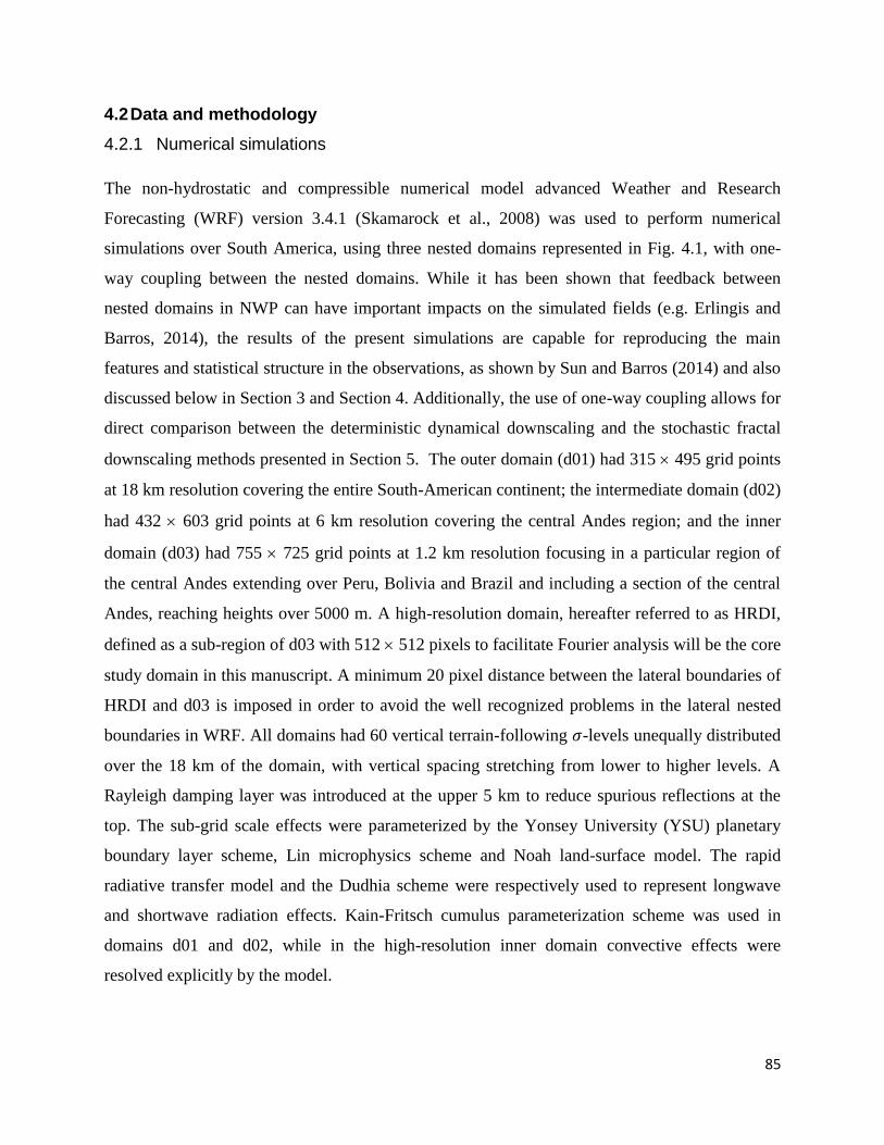
85
4.2 Data and methodology
4.2.1 Numerical simulations
The non-hydrostatic and compressible numerical model advanced Weather and Research
Forecasting (WRF) version 3.4.1 (Skamarock et al., 2008) was used to perform numerical
simulations over South America, using three nested domains represented in Fig. 4.1, with one-
way coupling between the nested domains. While it has been shown that feedback between
nested domains in NWP can have important impacts on the simulated fields (e.g. Erlingis and
Barros, 2014), the results of the present simulations are capable for reproducing the main
features and statistical structure in the observations, as shown by Sun and Barros (2014) and also
discussed below in Section 3 and Section 4. Additionally, the use of one-way coupling allows for
direct comparison between the deterministic dynamical downscaling and the stochastic fractal
downscaling methods presented in Section 5. The outer domain (d01) had 315 495 grid points
at 18 km resolution covering the entire South-American continent; the intermediate domain (d02)
had 432 603 grid points at 6 km resolution covering the central Andes region; and the inner
domain (d03) had 755 725 grid points at 1.2 km resolution focusing in a particular region of
the central Andes extending over Peru, Bolivia and Brazil and including a section of the central
Andes, reaching heights over 5000 m. A high-resolution domain, hereafter referred to as HRDI,
defined as a sub-region of d03 with 512 512 pixels to facilitate Fourier analysis will be the core
study domain in this manuscript. A minimum 20 pixel distance between the lateral boundaries of
HRDI and d03 is imposed in order to avoid the well recognized problems in the lateral nested
boundaries in WRF. All domains had 60 vertical terrain-following -levels unequally distributed
over the 18 km of the domain, with vertical spacing stretching from lower to higher levels. A
Rayleigh damping layer was introduced at the upper 5 km to reduce spurious reflections at the
top. The sub-grid scale effects were parameterized by the Yonsey University (YSU) planetary
boundary layer scheme, Lin microphysics scheme and Noah land-surface model. The rapid
radiative transfer model and the Dudhia scheme were respectively used to represent longwave
and shortwave radiation effects. Kain-Fritsch cumulus parameterization scheme was used in
domains d01 and d02, while in the high-resolution inner domain convective effects were
resolved explicitly by the model.
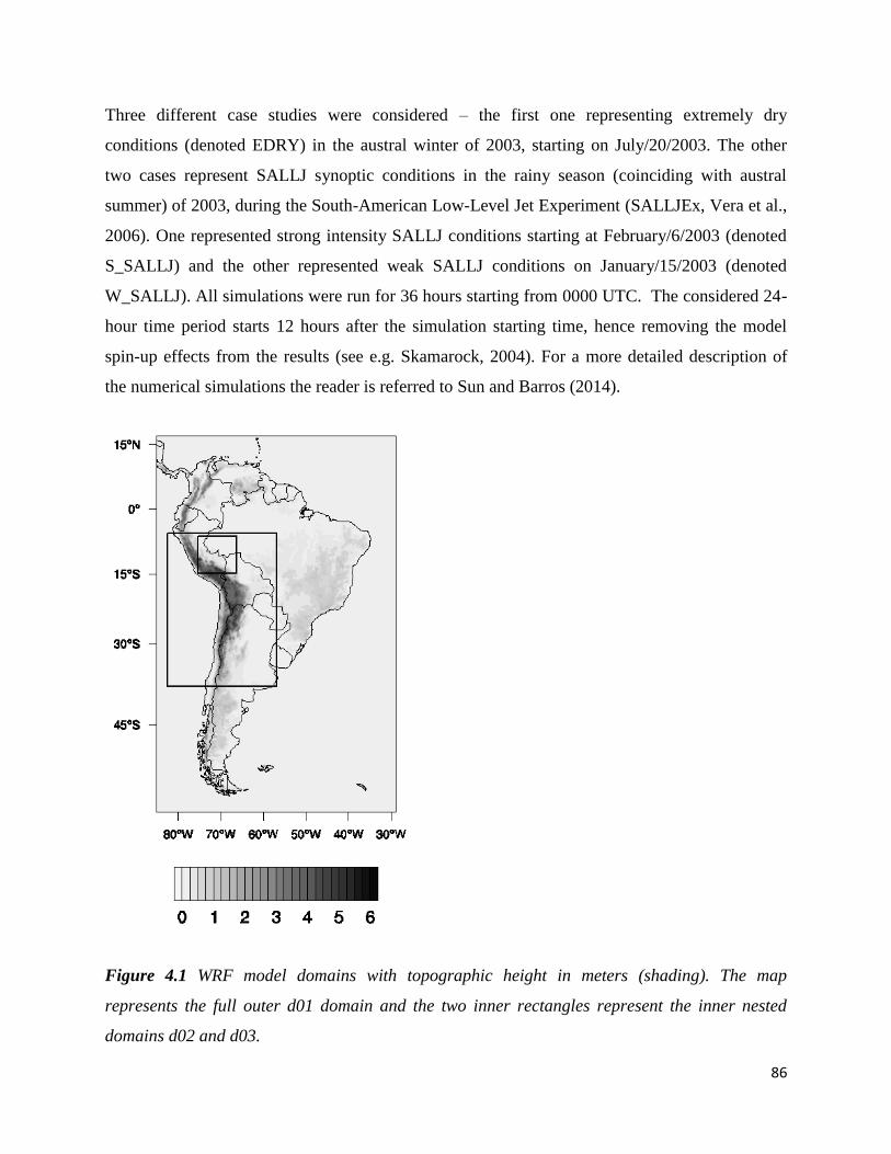
86
Three different case studies were considered – the first one representing extremely dry
conditions (denoted EDRY) in the austral winter of 2003, starting on July/20/2003. The other
two cases represent SALLJ synoptic conditions in the rainy season (coinciding with austral
summer) of 2003, during the South-American Low-Level Jet Experiment (SALLJEx, Vera et al.,
2006). One represented strong intensity SALLJ conditions starting at February/6/2003 (denoted
S_SALLJ) and the other represented weak SALLJ conditions on January/15/2003 (denoted
W_SALLJ). All simulations were run for 36 hours starting from 0000 UTC. The considered 24-
hour time period starts 12 hours after the simulation starting time, hence removing the model
spin-up effects from the results (see e.g. Skamarock, 2004). For a more detailed description of
the numerical simulations the reader is referred to Sun and Barros (2014).
Figure 4.1 WRF model domains with topographic height in meters (shading). The map
represents the full outer d01 domain and the two inner rectangles represent the inner nested
domains d02 and d03.
87
4.2.2 Multifractal framework
Gravity causes strong stratification and large aspect ratio in atmospheric flows over the meso-
and synoptic–scales of interest for weather and climate. This effectively rules out the existence
of isotropic turbulence regimes (e.g. Lovejoy and Schertzer, 2010b) and consequently
anisotropic behavior of the atmosphere must be considered with different scaling laws between
the horizontal and vertical directions:
(4.1)
Here, and represent fluctuations of a given scaling field respectively over
distance lengths and in the horizontal and vertical directions. and are the
corresponding conserved turbulent fluxes in the horizontal and vertical directions, and HH and Hv
are the respective non-conservation scaling parameter. Notice that the scale-by-scale conserved
property is the turbulent flux rather than the field F itself, with the H values measuring the
degree of non-conservation (H=0 for a conserved field). Based on classical turbulence theory, the
anisotropic generalized scale invariance framework (Schertzer and Lovejoy, 1985; Lovejoy and
Schertzer, 2010b) assumes that Kolmogorov (1941) scaling of turbulent velocity fluctuations
holds in the horizontal direction, the conserved cascade property being the turbulent energy flux,
and consequently HH=1/3. The assumption in the vertical direction is that
gravitational influence on buoyancy fluxes is the dominant process, with the buoyancy variance
flux being the conserved turbulent property following Bolgiano-Obukhov scaling (Bolgiano,
1959), , and consequently Hv=3/5. This implies that vertical sections of structures
become progressively flatter at larger and larger scales. The same HH and Hv exponents are
predicted for passive scalars, although the statistics should follow the Corssin-Obukhov scaling
for passive advection where the conserved turbulent fluxes are given by and
( represents the passive scalar variance flux, Lilley et al., 2004).

88
A further source of complexity comes from the fact that the statistics of the conserved turbulent
fluxes for atmospheric quantities are themselves scale dependent and exhibit multifractal
behavior following the generic scaling relationship (Schertzer and Lovejoy, 1987):
(4.2)
where the angle brackets represent the statistical average, q is the moment order generalized to
any positive real number, is the scale ratio, is the outer scale of the cascade and l the
scale of the observation. is the non-dimensional normalized turbulent flux measured at
resolution , such that . In multifractals, the scaling exponent function, K(q), is a
nonlinear convex function of q, and thus an infinity of exponents are required to characterize the
scaling behavior. This problem can be reduced to the determination of two parameters, and
C1, by using the universal multifractal (UM) framework (Schertzer and Lovejoy, 1987) where
K(q) given by:
(4.3)
The intermittency parameter, C1, describes the sparseness or non-homogeneity of the mean of the
process. The Levy index, , defined in the interval [0, 2], indicates the degree of multifractality,
with for monofractals. Both these parameters can be estimated using the Double Trace
Moment technique (DTM) described by Lavallée et al. (1993).
The Fourier spectral analysis is an alternative way to investigate the presence of scale invariant
behavior in atmospheric fields over a wide range of scales, manifested as log-log linearity of the
power spectrum:
(4.4)
with ki representing a 1-dimensional wavenumber. Eq. (4.4) has the advantage of representing a
simple framework that is familiar to atmospheric scientists and is quite sensitive to presence of
scaling behavior but also to scaling breaks and other types of deformations to the power law
behavior. The spectral exponent, , is related to UM parameters C1, and H (here it is assumed
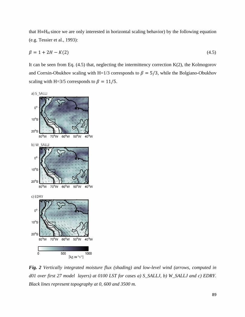
89
that HHH since we are only interested in horizontal scaling behavior) by the following equation
(e.g. Tessier et al., 1993):
(4.5)
It can be seen from Eq. (4.5) that, neglecting the intermittency correction K(2), the Kolmogorov
and Corrsin-Obukhov scaling with H=1/3 corresponds to , while the Bolgiano-Obukhov
scaling with H=3/5 corresponds to .
Fig. 2 Vertically integrated moisture flux (shading) and low-level wind (arrows, computed in
d01 over first 27 model layers) at 0100 LST for cases a) S_SALLJ, b) W_SALLJ and c) EDRY.
Black lines represent topography at 0, 600 and 3500 m.

90
Simulation
Daytime Nighttime
Pmax [mm/12hr] [mm/12hr]105 Pmax [mm/12hr] [mm/12hr]10
5
EDRY 0.3 0.00 0.1 0.00
W_SALLJ 173.6 8.47 276.2 7.22
S_SALLJ 118.8 3.46 87.8 1.80
Table 4.1 Local (pixel) maximum, Pmax, and total domain surface rainfall accumulated over 12
hour period during daytime (7 to 19 LST) and nighttime (19 to 7 LST) over the HRDI for EDRY,
W_SALLJ and S_SALLJ.
4.3 Central Andes simulation results
The presence of the South-Atlantic subtropical high causes a large-scale counterclockwise low-
level circulation transporting warm and moist unstable air from the tropical Atlantic Ocean and
the Amazon basin towards the Andes, a large-scale north-south orographic barrier with
elevations reaching 7 km. This westward moisture transport is verified in all three simulated
cases (EDRY, W_SALLJ and S_SALLJ) as illustrated in Fig. 4.2 by the large-scale low-level
flow (black arrows) together with the vertically integrated water vapor flux,
where g is the acceleration due to gravity, qv is the water vapor mixing
ratio, is the horizontal wind speed, and the pressure integral is taken between the
surface and the top model grid level. However, there are important differences in the large-scale
moisture flux patterns between the different cases with important consequences for orographic
rainfall. Cases under SALLJ conditions during the rainy season (S_SALLJ in Fig. 4.2a and
W_SALLJ in Fig. 4.2b) display much higher values toward the central Andes compared to
the dry season case EDRY (Fig. 4.2c). This pattern is maintained throughout the diurnal cycle as
shown by the total amount of water vapor upstream of the mountains (Fig. 4.3a), resulting in
very different total rainfall accumulations and local maximum rainfall over HRDI among the
different case studies (Table 4.1). Case EDRY has low moisture availability (Fig. 4.3a), weaker
upslope flows (Fig. 4.3b) and barely any CAPE (Fig. 4.3d) resulting in nearly zero atmospheric
condensate production (Fig. 4.3c) and no surface rainfall accumulation throughout the diurnal

91
cycle (Table 4.1). In contrast, cases W_SALLJ and S_SALLJ produce complex surface rainfall
accumulation patterns (Fig. 4.4) during day- (7 LST to 19 LST) and nighttime (19 LST to 7
LST). Several convective structures emerged along the eastern slopes and foothills of the Andes,
where the orographic perturbations play a crucial role in triggering deep convective throughout
the diurnal cycle together with the exponential decrease of saturation vapor pressure of the
atmosphere which also contributes to the larger probability of finding greater precipitation values
on the lower slopes of a high mountain (Houze, 2012). These results are in agreement with
Romatschke and Houze (2010) previous observations of deep convective precipitation over the
central Andes region under SALLJ conditions.
Figure 4.3 Diurnal cycles for the three case studies (EDRY, W_SALLJ and S_SALLJ) of a) total
water vapor mixing ratio available over HRDI upstream of the Andes eastern flanks (at
topographic height below 600 m); b) mean y-direction wind component, v, at low-levels (first 27
model layers) upstream of the Andes eastern flanks; c) total condensate mixing rate over HRDI;
d) mean CAPE over HRDI.

92
Figure 4.4 Simulated mean hourly rainfall rate during daytime (7 to 19 LST) for case a)
W_SALLJ and c) S_SALLJ; and during nighttime (19 to 7 LST) for case b) W_SALLJ and d)
S_SALLJ. The black solid lines represent topographic elevation at 600 and 3500 m.
The most intense rainfall patterns throughout the diurnal cycle were found under weak SALLJ
conditions, when the low-level jet withdraws to the north (see Fig. 4.3 and Table 4.1), also in
agreement with Romatschke and Houze (2010). This is explained by the more intense upslope
moisture fluxes in the W_SALLJ case compared to S_SALLJ, with larger magnitude of the
upslope flow (Fig. 4.3b) and larger moisture availability during the morning hours (Fig. 4.3a)
resulting in stronger orographic triggering and enhancing of convection with associated larger
and faster consumption of CAPE (Fig. 4.3d) causing proportionally large peaks in atmospheric
condensation (Fig. 4.3c). The peak local rainfall accumulation occurs during the nighttime in
case W_SALLJ with an increase of nearly 60% compared to the daytime peak (Table 4.),
corresponding to the large intense structure over the south-east corner of Fig. 4.4b. This result
contrasts with more modest daytime peaks of CAPE consumption (Fig. 4.3d) and atmospheric

93
condensate production (Fig. 4.3c). During daytime there is a layer of low-level strongly unstable
moist flow impinging upon the Andes eastern flanks, with higher equivalent potential
temperature, , than the above mid-altitude air (Fig. 4.5a). This strong instability tends to be
released at first opportunity upon impinging on the foothills of the Andes (Houze, 2012),
resulting in transient and intermittent condensation patterns. During the nighttime the upslope
low-level flow is still strongly unstable with mean CAPE values over 1000 J/kg (Fig. 3d), despite
the decreases in the strength of the vertical gradient (Fig. 5b). Additionally there is a nocturnal
intensification of the upslope flow (Fig. 3c) which interacts with the local nighttime downslope
mountain breeze to reinforce convection (as exemplified in Fig. 5b). The result is the nighttime
generation of more organized and larger deep convective precipitation features with more
persistent spatial distributions, responsible for the higher local rainfall accumulations.
Figure 4.5 Case W_SALLJ y-z cross sections of equivalent potential temperature (colorscale)
and v-w flow (arrows) crossing the Andes at a) 1600 LST and b) 0400 LST. Dashed countour
lines represent atmospheric condensate mixing ratio concentrations of 1 g/kg.
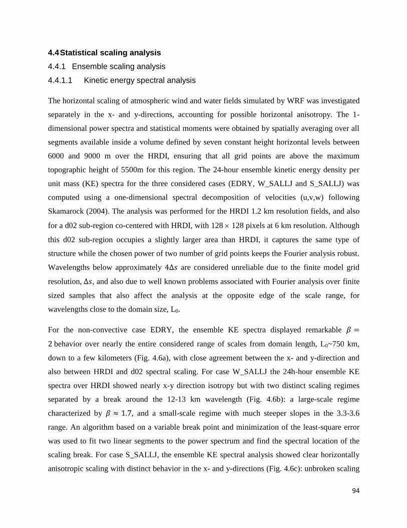
94
4.4 Statistical scaling analysis
4.4.1 Ensemble scaling analysis
4.4.1.1 Kinetic energy spectral analysis
The horizontal scaling of atmospheric wind and water fields simulated by WRF was investigated
separately in the x- and y-directions, accounting for possible horizontal anisotropy. The 1-
dimensional power spectra and statistical moments were obtained by spatially averaging over all
segments available inside a volume defined by seven constant height horizontal levels between
6000 and 9000 m over the HRDI, ensuring that all grid points are above the maximum
topographic height of 5500m for this region. The 24-hour ensemble kinetic energy density per
unit mass (KE) spectra for the three considered cases (EDRY, W_SALLJ and S_SALLJ) was
computed using a one-dimensional spectral decomposition of velocities (u,v,w) following
Skamarock (2004). The analysis was performed for the HRDI 1.2 km resolution fields, and also
for a d02 sub-region co-centered with HRDI, with 128 128 pixels at 6 km resolution. Although
this d02 sub-region occupies a slightly larger area than HRDI, it captures the same type of
structure while the chosen power of two number of grid points keeps the Fourier analysis robust.
Wavelengths below approximately are considered unreliable due to the finite model grid
resolution, , and also due to well known problems associated with Fourier analysis over finite
sized samples that also affect the analysis at the opposite edge of the scale range, for
wavelengths close to the domain size, L0.
For the non-convective case EDRY, the ensemble KE spectra displayed remarkable
behavior over nearly the entire considered range of scales from domain length, L0~750 km,
down to a few kilometers (Fig. 4.6a), with close agreement between the x- and y-direction and
also between HRDI and d02 spectral scaling. For case W_SALLJ the 24h-hour ensemble KE
spectra over HRDI showed nearly x-y direction isotropy but with two distinct scaling regimes
separated by a break around the 12-13 km wavelength (Fig. 4.6b): a large-scale regime
characterized by , and a small-scale regime with much steeper slopes in the 3.3-3.6
range. An algorithm based on a variable break point and minimization of the least-square error
was used to fit two linear segments to the power spectrum and find the spectral location of the
scaling break. For case S_SALLJ, the ensemble KE spectral analysis showed clear horizontally
anisotropic scaling with distinct behavior in the x- and y-directions (Fig. 4.6c): unbroken scaling
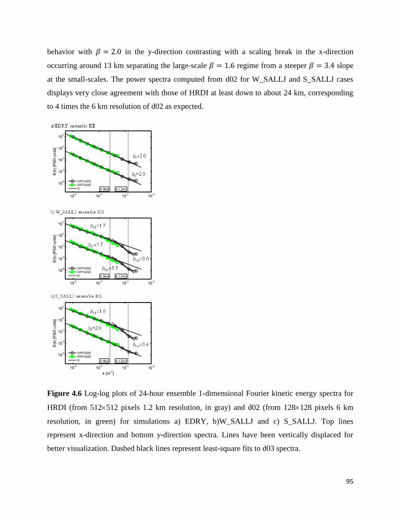
95
behavior with in the y-direction contrasting with a scaling break in the x-direction
occurring around 13 km separating the large-scale regime from a steeper slope
at the small-scales. The power spectra computed from d02 for W_SALLJ and S_SALLJ cases
displays very close agreement with those of HRDI at least down to about 24 km, corresponding
to 4 times the 6 km resolution of d02 as expected.
Figure 4.6 Log-log plots of 24-hour ensemble 1-dimensional Fourier kinetic energy spectra for
HRDI (from 512512 pixels 1.2 km resolution, in gray) and d02 (from 128128 pixels 6 km
resolution, in green) for simulations a) EDRY, b)W_SALLJ and c) S_SALLJ. Top lines
represent x-direction and bottom y-direction spectra. Lines have been vertically displaced for
better visualization. Dashed black lines represent least-square fits to d03 spectra.
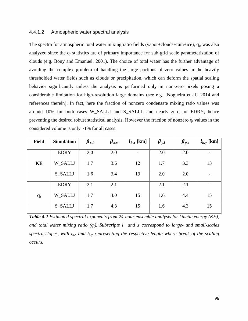
96
4.4.1.2 Atmospheric water spectral analysis
The spectra for atmospheric total water mixing ratio fields (vapor+clouds+rain+ice), qt, was also
analyzed since the qt statistics are of primary importance for sub-grid scale parameterization of
clouds (e.g. Bony and Emanuel, 2001). The choice of total water has the further advantage of
avoiding the complex problem of handling the large portions of zero values in the heavily
thresholded water fields such as clouds or precipitation, which can deform the spatial scaling
behavior significantly unless the analysis is performed only in non-zero pixels posing a
considerable limitation for high-resolution large domains (see e.g. Nogueira et al., 2014 and
references therein). In fact, here the fraction of nonzero condensate mixing ratio values was
around 10% for both cases W_SALLJ and S_SALLJ, and nearly zero for EDRY, hence
preventing the desired robust statistical analysis. However the fraction of nonzero qt values in the
considered volume is only ~1% for all cases.
Field Simulation [km] [km]
KE
EDRY 2.0 2.0 - 2.0 2.0 -
W_SALLJ 1.7 3.6 12 1.7 3.3 13
S_SALLJ 1.6 3.4 13 2.0 2.0 -
qt
EDRY 2.1 2.1 - 2.1 2.1 -
W_SALLJ 1.7 4.0 15 1.6 4.4 15
S_SALLJ 1.7 4.3 15 1.6 4.3 15
Table 4.2 Estimated spectral exponents from 24-hour ensemble analysis for kinetic energy (KE),
and total water mixing ratio (qt). Subscripts and correspond to large- and small-scales
spectra slopes, with lb,x and lb,y representing the respective length where break of the scaling
occurs.

97
Figure 4.7 Log-log plot of 24-hour ensemble 1-dimensional qt Fourier spectra for HRDI (from
512512 pixels 1.2 km resolution, in gray) and d02 (from 128128 pixels 6 km resolution, in
green) for simulations a) EDRY, b)W_SALLJ and c) S_SALLJ. Red line represents power spectra
from NCEP CPC brightness temperatures <250 K fields. Top lines represent x-direction and
bottom y-direction spectra. Lines have been vertically displaced for better visualization. Dashed
black lines represent least-square fits to d03spectra.
The 24-hour ensemble power spectra of qt are tightly connected to the results obtained for KE:
case EDRY shows unbroken scaling behavior with (Fig. 4.7a), while a scaling break
around 15 km was found in both W_SALLJ (Fig. 4.7b) and S_SALLJ cases (Fig. 4.7c)
separating the large-scale regime with slopes from a much steeper small-scale
slopes with values >4. Total water fields also display very good agreement in the spectra

98
obtained from d02 and HRDI with nearly horizontally isotropic behavior for EDRY and
W_SALLJ cases. The main difference between KE and qt occurs for case S_SALLJ where nearly
horizontally isotropic scaling was obtained in contrast to the anisotropic behavior in the former
(see Table 4.2).
The scaling derived from NCEP Climate Prediction Center (NCEP/CPC) globally merged
infrared product at 4 km is used to inform on the scale-invariant behavior of the real atmosphere
under convective conditions. Following Nesbitt et al., (2000), satellite measured brightness
temperatures below 250K are used to identify convective structures. The scaling behavior of
such convective structures (red lines in Fig. 4.7a and Fig. 4.7b) matches the simulated spectra of
both W_SALLJ and S_SALLJ. Under dry conditions, when atmospheric condensate is nearly
absent such analysis from brightness temperatures is not possible. The robustness of the
simulated large-scale scaling behavior is further supported by the simulations ability to
reproduce the main features observed over the central Andes under respective synoptic
conditions as discussed in Section 3, and also in Sun and Barros (2014).
Similar scaling breaks separating a shallower large-scale linear behavior from an abrupt
steepening at small-scales were previously observed in high-resolution NWP simulations of
convective storms for ensemble KE spectra (Skamarock, 2004) and hourly rainfall spectra
(Harris et al., 2001), who also found similarity between the large-scale simulated and observed
spectra down to the model effective resolution. The model effective resolution was defined by
Skamarock (2004) as the wavelength separating the large-scale scaling behavior in good
agreement with observations of the atmosphere from a spurious spectral steepening at smaller
wavelengths, reaching unphysical values of . Also, Skamarock (2004) showed that the
steepening is caused by the underrepresentation of small-scale variability associated with the
numerical integration over a finite grid with finite resolution, and the smoothing artifacts of the
subgrid-turbulence mixing parameterization and (unphysical) numerical diffusion schemes
introduced to maintain the numerical simulations stable. Hence the effective resolution was
shown to depend on the particular physical options of the NWP model. In the present work, the
effective resolution is shown to also be dependent on the particular flow regime. Under
convective conditions, the effective resolution estimated here at 1.2 km resolution is between
10 and 14 , much larger than the typically 4-5 values typically considered for numerical
99
simulations. An important implication of these results is that the effective improvement in
resolution associated with the nested dynamical downscaling between 6- and 1.2-km resolutions
is on the order of 2 or lower (between the effective resolutions of 25-30km in d02 and 10-16 km
in d03), hence much smaller than the 5 ratio between the respective grid resolutions.
4.4.1.3 Moment scaling analysis
Ensemble horizontal 1-directional moment scaling analysis of HRDI KE (Fig. 4.8a) and qt (Fig.
4.9a) fields under dry conditions (EDRY) showed remarkable unbroken multifractal behavior up
to moment orders of 3 over the scale range of interest, from scales near L0 down to
approximately . For convective cases, under SALLJ synoptic conditions the multifractal
scaling behavior was found at large-scales above to the scaling break length estimated in the
spectral analysis, and non-scaling behavior was obtained at smaller-scales below the break length
scale (Fig. 4.8b and Fig 4.8c for KE fields, and Fig. 4.9b and Fig. 4.9c for qt). Table 4.3 presents
the UM parameters C1 and estimated for the large-scales (using the break length scales
obtained in the spectral analysis) using the DTM technique. For both KE and qt, the estimated
intermittency parameters C1 in the x- and y-directions were lower (0.07-0.10) in the non-
convective dry scenario (EDRY) as compared to (0.13-0.20) for deep convective cases
(W_SALLJ and S_SALLJ). This increased intermittency in convective cases is intuitive given
the presence of strong localized convective updrafts and associated increased atmospheric
condensation. The multifractal parameter varies in the range 1.5-2.0, with slightly lower values
in EDRY case for KE and qt but without any clear tendency between the distinct simulations.
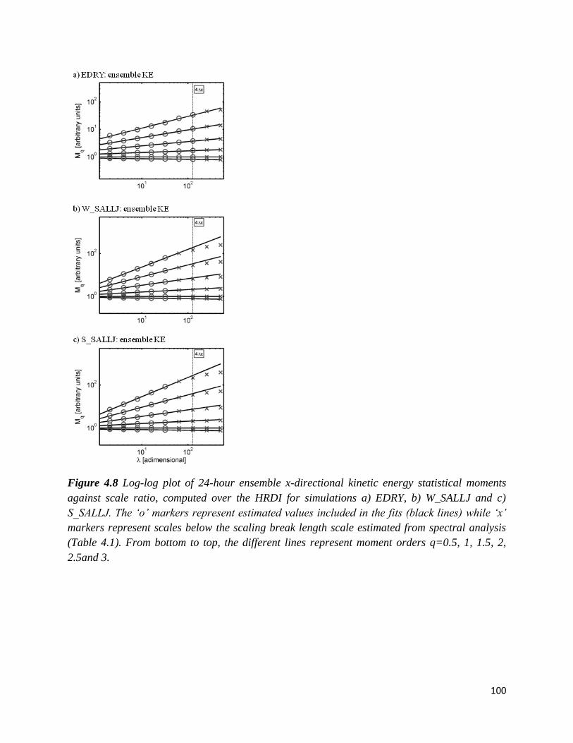
100
Figure 4.8 Log-log plot of 24-hour ensemble x-directional kinetic energy statistical moments
against scale ratio, computed over the HRDI for simulations a) EDRY, b) W_SALLJ and c)
S_SALLJ. h ‘o’ ark rs r r s t sti at va u s i u i th fits (b a k i s) whi ‘x’
markers represent scales below the scaling break length scale estimated from spectral analysis
(Table 4.1). From bottom to top, the different lines represent moment orders q=0.5, 1, 1.5, 2,
2.5and 3.

101
Figure 4.9 Same as Fig. 4.8 but computed from qt fields.
In summary the ensemble scaling analysis reveals that WRF simulated fields are able to
reproduce the scaling behavior in atmospheric observations down to the model effective
resolution, below which the statistical structure is misrepresented by the model due to finite grid
spacing, deficiencies in the used sub-grid scale parameterizations and the (unphysical) numerical
diffusion introduced to keep the simulations stable. A fundamental transition was found in the
scaling behavior of atmospheric wind and water fields between non-convective and convective
regimes. Additionally, in the convective regime the HRDI effective resolution shifts to length
scales well above 4-5 , causing a significant decrease in the resolution gain when the grid-
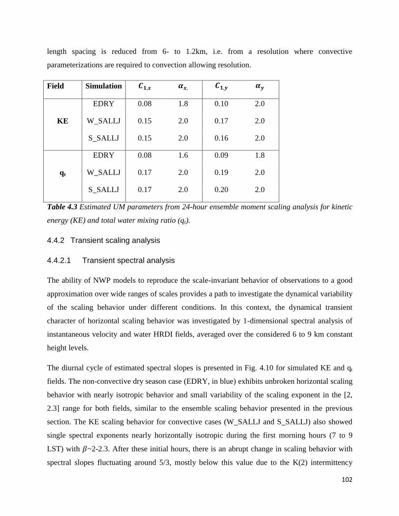
102
length spacing is reduced from 6- to 1.2km, i.e. from a resolution where convective
parameterizations are required to convection allowing resolution.
Field Simulation
KE
EDRY 0.08 1.8 0.10 2.0
W_SALLJ 0.15 2.0 0.17 2.0
S_SALLJ 0.15 2.0 0.16 2.0
qt
EDRY 0.08 1.6 0.09 1.8
W_SALLJ 0.17 2.0 0.19 2.0
S_SALLJ 0.17 2.0 0.20 2.0
Table 4.3 Estimated UM parameters from 24-hour ensemble moment scaling analysis for kinetic
energy (KE) and total water mixing ratio (qt).
4.4.2 Transient scaling analysis
4.4.2.1 Transient spectral analysis
The ability of NWP models to reproduce the scale-invariant behavior of observations to a good
approximation over wide ranges of scales provides a path to investigate the dynamical variability
of the scaling behavior under different conditions. In this context, the dynamical transient
character of horizontal scaling behavior was investigated by 1-dimensional spectral analysis of
instantaneous velocity and water HRDI fields, averaged over the considered 6 to 9 km constant
height levels.
The diurnal cycle of estimated spectral slopes is presented in Fig. 4.10 for simulated KE and qt
fields. The non-convective dry season case (EDRY, in blue) exhibits unbroken horizontal scaling
behavior with nearly isotropic behavior and small variability of the scaling exponent in the [2,
2.3] range for both fields, similar to the ensemble scaling behavior presented in the previous
section. The KE scaling behavior for convective cases (W_SALLJ and S_SALLJ) also showed
single spectral exponents nearly horizontally isotropic during the first morning hours (7 to 9
LST) with ~2-2.3. After these initial hours, there is an abrupt change in scaling behavior with
spectral slopes fluctuating around 5/3, mostly below this value due to the K(2) intermittency

103
correction (see Eq. 4.5). Horizontal isotropy holds to a good approximation throughout most of
the day for case W_SALLJ, with similar trends in the x- and y-direction conserving the
differences below 0.25 which cannot be distinguished from the typical uncertainty in the
estimation of for single instantaneous fields (e.g. Barros et al., 2004). The only exceptions
occurring in the early morning (6 to 7 LST in the next morning) larger x-y anisotropy is found in
the KE spectra, with x-direction statistics displaying broken 5/3 behavior while unbroken
behavior with steeper slopes around 2 is found in the y-direction. In contrast, KE spectra for case
S_SALLJ display horizontally anisotropic behavior throughout most of the day, with unbroken
scaling in the y-direction and broken in the x-direction in agreement with the result
obtained from ensemble scaling analysis in Section 4.4.1.
Figure 4.10 Diurnal cycle of transient spectral exponent computed from instantaneous fields in
the x- (solid line) and y-direction (dashed line) for cases EDRY (blue), W_SALLJ (red) and
S_SALLJ (green) for a) KE and b) qt. Unbroken scaling behavior over scale range between L0
and 4 x is si a by ‘o’ ark rs whi brok s a i b havior is si a by ‘x’ ark rs,
with the value represented in the latter case corresponding to the large-scale scaling behavior.
Total water mixing ratio fields (Fig. 4.10b) from case W_SALLJ display a generally similar
diurnal cycle to KE, including a similar transition between unbroken ~2-2.2 spectra in the non-
convective regime to a broken scaling with decreased slopes around 5/3 at the large-scales when
convection sets in. This transition was also present in S_SALLJ qt fields, but in contrast to KE
transient scaling for total water case S_SALLJ remains mostly horizontally isotropic except in
the early morning at the end of the study time-period, where significant anisotropy emerges.
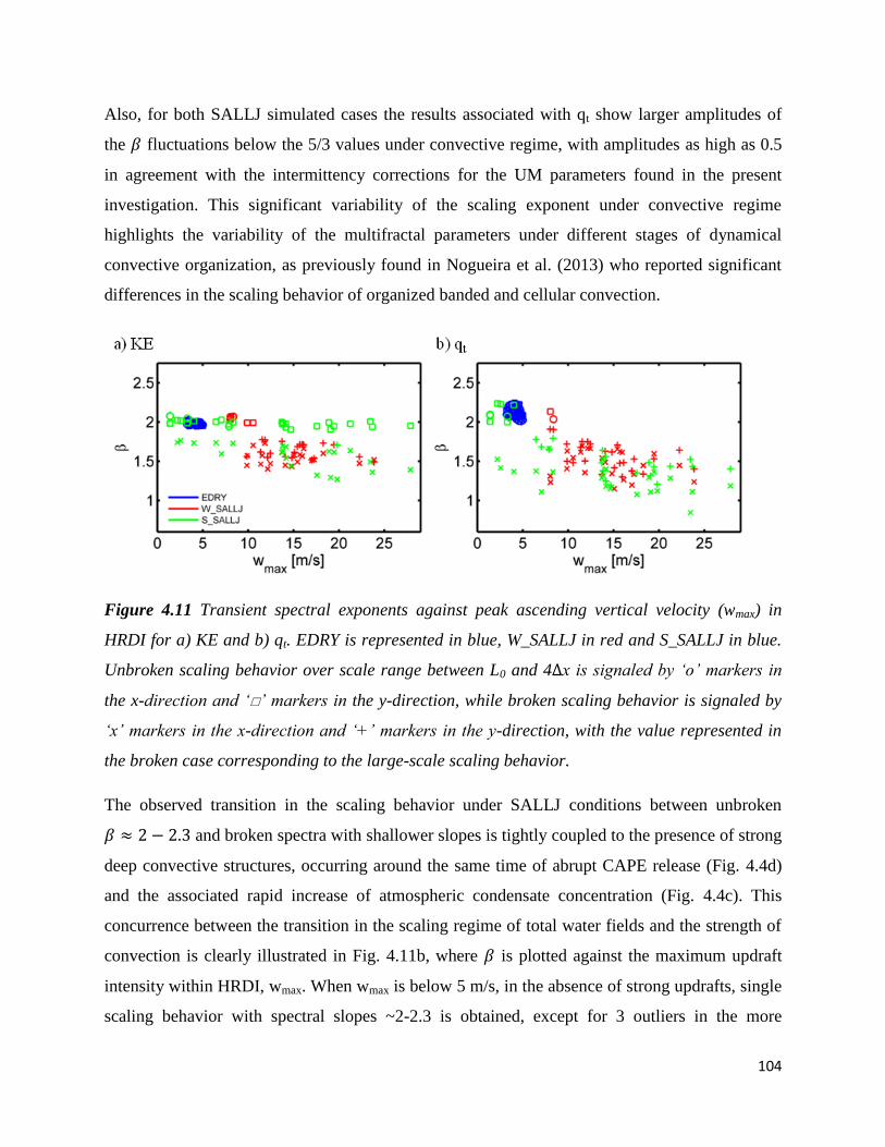
104
Also, for both SALLJ simulated cases the results associated with qt show larger amplitudes of
the fluctuations below the 5/3 values under convective regime, with amplitudes as high as 0.5
in agreement with the intermittency corrections for the UM parameters found in the present
investigation. This significant variability of the scaling exponent under convective regime
highlights the variability of the multifractal parameters under different stages of dynamical
convective organization, as previously found in Nogueira et al. (2013) who reported significant
differences in the scaling behavior of organized banded and cellular convection.
Figure 4.11 Transient spectral exponents against peak ascending vertical velocity (wmax) in
HRDI for a) KE and b) qt. EDRY is represented in blue, W_SALLJ in red and S_SALLJ in blue.
Unbroken scaling behavior over scale range between L0 and 4 x is si a by ‘o’ ark rs i
the x- ir tio a ‘’ ark rs i the y-direction, while broken scaling behavior is signaled by
‘x’ ark rs i th x- ir tio a ‘ ’ ark rs i th y-direction, with the value represented in
the broken case corresponding to the large-scale scaling behavior.
The observed transition in the scaling behavior under SALLJ conditions between unbroken
and broken spectra with shallower slopes is tightly coupled to the presence of strong
deep convective structures, occurring around the same time of abrupt CAPE release (Fig. 4.4d)
and the associated rapid increase of atmospheric condensate concentration (Fig. 4.4c). This
concurrence between the transition in the scaling regime of total water fields and the strength of
convection is clearly illustrated in Fig. 4.11b, where is plotted against the maximum updraft
intensity within HRDI, wmax. When wmax is below 5 m/s, in the absence of strong updrafts, single
scaling behavior with spectral slopes ~2-2.3 is obtained, except for 3 outliers in the more
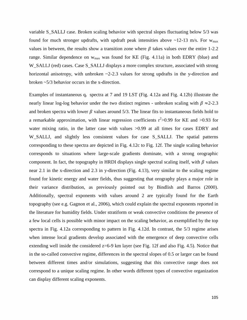
105
variable S_SALLJ case. Broken scaling behavior with spectral slopes fluctuating below 5/3 was
found for much stronger updrafts, with updraft peak intensities above ~12-13 m/s. For wmax
values in between, the results show a transition zone where takes values over the entire 1-2.2
range. Similar dependence on wmax was found for KE (Fig. 4.11a) in both EDRY (blue) and
W_SALLJ (red) cases. Case S_SALLJ displays a more complex structure, associated with strong
horizontal anisotropy, with unbroken ~2-2.3 values for strong updrafts in the y-direction and
broken ~5/3 behavior occurs in the x-direction.
Examples of instantaneous qt spectra at 7 and 19 LST (Fig. 4.12a and Fig. 4.12b) illustrate the
nearly linear log-log behavior under the two distinct regimes - unbroken scaling with 2-2.3
and broken spectra with lower values around 5/3. The linear fits to instantaneous fields hold to
a remarkable approximation, with linear regression coefficients r2>0.99 for KE and >0.93 for
water mixing ratio, in the latter case with values >0.99 at all times for cases EDRY and
W_SALLJ, and slightly less consistent values for case S_SALLJ. The spatial patterns
corresponding to these spectra are depicted in Fig. 4.12c to Fig. 12f. The single scaling behavior
corresponds to situations where large-scale gradients dominate, with a strong orographic
component. In fact, the topography in HRDI displays single spectral scaling itself, with values
near 2.1 in the x-direction and 2.3 in y-direction (Fig. 4.13), very similar to the scaling regime
found for kinetic energy and water fields, thus suggesting that orography plays a major role in
their variance distribution, as previously pointed out by Bindlish and Barros (2000).
Additionally, spectral exponents with values around 2 are typically found for the Earth
topography (see e.g. Gagnon et al., 2006), which could explain the spectral exponents reported in
the literature for humidity fields. Under stratiform or weak convective conditions the presence of
a few local cells is possible with minor impact on the scaling behavior, as exemplified by the top
spectra in Fig. 4.12a corresponding to pattern in Fig. 4.12d. In contrast, the 5/3 regime arises
when intense local gradients develop associated with the emergence of deep convective cells
extending well inside the considered z=6-9 km layer (see Fig. 12f and also Fig. 4.5). Notice that
in the so-called convective regime, differences in the spectral slopes of 0.5 or larger can be found
between different times and/or simulations, suggesting that this convective range does not
correspond to a unique scaling regime. In other words different types of convective organization
can display different scaling exponents.

106
Figure 4.12 Log-log plots of vertically averaged instantaneous qt horizontal spectra (gray) for
simulation a) EDRY, b) W_SALLJ, with top line at 07LST and bottom at 19LST. Black dashed
line is least square fit. Horizontal maps of qt vertically integrated qt over z=6-9km at 07LST and
19LST respectively for c) and e) EDRY and d) and f) W_SALLJ.

107
Figure 4.13 Log-log power spectra computed from topographic elevation over HRDI (light grey)
and d02 (dark grey) and the respective least square fit (black dashed line). Vertical black thin
lines represent the 4 times grid resolution scales for d02 and HRDI.
4.4.2.2 Transient moment scaling analysis
Scaling also holds to a very good approximation for the statistical moments of instantaneous
water and kinetic energy fields, with small variations about the log-log linear (power law)
relationships with scale. The transition between weak and strong updrafts is also present when
the statistical moments are analyzed (Fig. 4.14), with single scaling behavior and lower
intermittency ( ) for wmax<5-7 m/s and broken scaling with higher intermittency
for strong updrafts, wmax>10-15 m/s. As pointed out for the ensemble moment scaling analysis,
the increased intermittency in convective regimes is expected due to emergence of localized
intense cellular features compared to the smoother stratiform patterns. Between these two ranges
there is a transition zone where C1 increases approximately linearly. Similar to the results
obtained for the ensemble analysis in Section 4.4.1, UM parameter does not show any clear
tendencies for the transition between non-convective and convective regimes (Fig. 4.15)
statistics.
In summary, scaling behavior holds to a remarkable approximation in numerically simulated
instantaneous atmospheric wind and water fields. This scale-invariant behavior is intrinsically
transient, characterized by scaling parameters that dynamically depend on the atmospheric state.
In particular, a robust transition was found in parameters and C1 between non-convective and

108
convective regimes. Because the high-resolution NWP simulations are obtained under fully
realistic configurations, capable of representing the observed atmospheric behavior down to the
model effective resolution, the present results extend the previous results of Nogueira et al.
(2013) that found similar non-convective/convective transitions for rainfall and cloud fields
obtained from highly idealized simulations of orographic convection at 250m resolution.
Figure 4.14 Transient intermittency parameter, C1, against maximum ascending vertical velocity
(wmax) in HRDI for a) KE and b) qt. EDRY is represented in blue, W_SALLJ in red and S_SALLJ
in blue.
Figure 4.15 Transient multifractal parameter, , against maximum ascending vertical velocity
(wmax) in HRDI for a) KE and b) qt. EDRY is represented in blue, W_SALLJ in red and S_SALLJ
in blue.
109
4.5 Sub-grid scale statistics of atmospheric moisture
Cloud fraction, cf, is a key variable in the sub-grid parameterization of clouds in NWP,
representing the relative volumes of clear-sky and clouds inside a certain large-scale domain,
which can be a coarse resolution grid volume or any other convenient domain of choice. In other
words, the cloud fraction parameter describes the spatial distribution of condensed water within
this domain. Cloud fraction can be equivalently defined as the fraction of horizontal area under
the simplifying assumption that water fields are homogeneous along the vertical direction inside
a grid-box, based on a smaller vertical grid spacing of the numerical simulations (in the order of
100 m) compared to the horizontal grid spacing (1.2 km in the highest resolution domain).
Following Bony and Emanuel (2001) the probability distribution function (PDF) of total water
mixing ratio
, can be used to represent stochastically the cloud fraction
within a model grid-box as
, where qs is the saturation mixing rate, that can be
diagnosed from the coarse resolution temperature and pressure fields. Consequently, the
determination of the sub-grid probability distribution of total water mixing ratio is a question of
primary importance for the stochastic parameterization of clouds.
Bony and Emanuel (2001) assumed a generalized log-normal form to model P(qt) which might
not be ideal for multifractal fields as argued in Section 4.1. Here the ability of statistical scale-
invariant behavior to represent the sub-grid scale qt PDF was investigated by using a stochastic
modified fractal interpolation algorithm to generate an ensemble of plausible qt fields at the
desired resolution based on the known coarse resolution information alone. These fractal
downscaling methods work in the Fourier spectral framework, assuming horizontal isotropy for
simplicity to generate 2-dimensional fractional Brownian surfaces with the desired spectral
slope, which are then used as spatial interpolating surfaces. Detailed descriptions of the
algorithm and performance evaluations can be found in Bindlish and Barros (1996, 2000),
Rebora et al. (2006), Tao and Barros (2010) and Nogueira and Barros (2014). In analogy with
the dynamical downscaling undertaken with nested domains in WRF, the resolution increase
occurs only in the horizontal directions, while in the vertical the much higher resolution of the
numerical grid is kept unchanged. Notice that to extend the downscaling to the vertical direction
the horizontal-vertical anisotropy must be taken into consideration as discussed in Section 4.1
and Section 4.2.
110
Previous research demonstrated that the fractal methods used here are able to accurately preserve
the coarse resolution structure while enhancing the variability at the sub-grid scales, and can
rapidly produce a large number of statistically coherent high-resolution realizations of the field.
In particular Nogueira and Barros (2014) showed that downscaled realizations of observed
precipitation fields generated by fractal methods can be used to produce accurate stochastic
predictions of streamflow in hydrological simulations representing a considerable improvement
in prediction accuracy compared to other interpolation methods. It is important to stress that such
fractal downscaling methods require the a priori knowledge of the spectral exponent, which is
far from being a trivial problem when the transient scaling behavior is taken into account, as
pointed out in Nogueira et al. (2013) who found complex non-linear transitions in the scaling
behavior between different flow regimes, with dynamical dependencies on several large-scale
properties including atmospheric stability, mean wind speed and orographic forcing. The
transient scaling parameters can potentially be estimated directly from the instantaneous coarse
resolution field, as done in Nogueira et al. (2014). However, for limited-area domains the
information in instantaneous coarse resolution fields is generally not sufficient to obtain direct
robust estimates of the scaling parameters.
Fractal downscaling methods combining coarse resolution observations and high-resolution
ancillary data have been proposed for remote sensing applications (Kim and Barros, 2002;
Barros and Tao, 2008). In the general case, such ancillary fields will not be available at the
resolutions required for cloud parameterization and for prognostic applications, and hence a
strategy based on coarse resolution information alone is preferred. An alternative method is
presented here based on the non-convective/convective scaling transition. Whereas a nonlinear
fit to the spectral slope dependencies in Figs. 4.10 and 4.11 is possible, the limited number of
cases studied in this manuscript prevents the estimation of general relationships. Thus, a first-
order assumption is made by taking for non-convective cases and for
convective cases (representing the 5/3 regime with intermittency correction), corresponding to
the respective mean spectral slopes estimated from instantaneous qt statistics for the three
considered simulated cases in Section 4.4.2.

111
Figure 4.16 Probability distribution function computed from HRDI (black circle markers) and
0 (b a k ‘x’ ark rs) for si u atio EDRY ( ft o u ), W_SALLJ ( i o u ) a
S_SALLJ (right column) in the period 7-9 LST (top row), 12-14 LST (middle row) and 17-19
(bottom row). Green line represents the lognormal distribution estimated from d02 fields over
the same period and simulation. Red (blue) lines represent lower and higher PDF limits
estimated using an ensemble of 50 fractal downscaled realizations from d02 fields at 6km
resolution to 1.2km resolution considering a spectral slope =1.5 ( =2.1).
The PDFs obtained directly from the WRF simulated qt fields over the HRDI region at 6- and at
1.2 km resolution are shown by black lines in Fig. 4.16 for the 3 simulations. The results display
clearly distinct shapes of the PDF between the different simulated cases. Case EDRY displays
higher probabilities associated with qt values g/kg and maximum intensities below 5 g/kg
(Fig. 4.16a to Fig. 4.16c). In the most intense convective case W_SALLJ the higher probabilities

112
are associated with qt values in the [1,5] g/kg range and maximum intensities can reach values
around 15 g/kg when deep convective structures form during the afternoon (Fig. 4.16e and Fig.
4.16f). Finally, case S_SALLJ displays high probabilities associated with low qt ( g/kg), but
also reaching high intensities around 15 g/kg. The respective PDFs estimated for each case using
log-normal statistics are represented by green lines in Fig. 4.16, with the statistical moments
estimated directly from the 1.2 km HRDI domain, hence representing a best case scenario where
the high-resolution statistics are known exactly. Note that, in the general case, the high-
resolution must be estimated from the coarse resolution information alone introducing further
uncertainties to the log-normal PDFs. The blue (red) lines in Fig. 4.16 represent the PDFs
estimated from the fractal downscaling from 6- to 1.2-km resolution considering
( ). The two lines for each case mark the limits of the ensemble spread of PDF resulting
from 50 realizations, hence representing the range of possible solutions given by the fractal
downscaling algorithm including the associated uncertainty. While the log-normal statistics can
capture the essential shape of the PDF, they overestimate the probabilities over the dominant
ranges (most probable intensities) in all cases, and largely overestimate the probabilities
associated with higher intensities in the EDRY (Fig. 4.16a-c) and underestimate the high
intensity tails in the convective cases (Fig. 4.16e,f,h,i). The fractal downscaling solutions
capture the most probable range of values in all cases independently of the chosen scaling
exponent. The ability of the fractal scheme to conserve the coarse resolution structure has a large
contribution to this very good fit, since the differences between 6- and 1.2-km PDFs in this
interval of values are small.
The present analysis is limited by the errors associated with the misrepresentation of the
statistical structure in the high-resolution simulated fields, as discussed in Section 4.
Nonetheless, the fractal downscaling scheme is capable of capturing important properties of the
expected PDF behavior when increasing resolution: on the one hand by taking the
results capture the PDFs for cases where the distribution changes slowly with increasing
resolution, typical in the less intermittent non-convective cases; on the other hand the 1.5 spectral
slopes represent convective situations where there is a sharp increase in the high-values tail and a
corresponding increase in the low-value end, caused by mass conservation. Overall, the high-
resolution PDF can be found within the ensemble spread of fractal solutions. Consequently these
results provide a basis for stochastic sub-grid parameterization of cloud fraction in prognostic
113
applications relying on simulated fields only, and it that can easily be generalized for any scaling
geophysical fields given that the respective spectral exponents can be estimated. The fractal
downscaling solutions with the regime-based spectral slope approximations provide
computationally affordable alternatives for real-time applications, and can be also useful when
coarse resolution fields do not have enough information to characterize their scaling behavior
(i.e. limited area domains, very large scale ratios).
4.6 Conclusions
High-resolution one-way nested simulations performed with WRF model over the central Andes
region were able to accurately reproduce the main features of observed rainy season orographic
deep convective events and dry season conditions (Sun and Barros, 2014). The typically
observed horizontal scaling behavior of atmospheric fields over wide ranges of scales was also
captured by the numerical simulated wind and atmospheric water content fields down to the
model effective resolution, which is a transient length-scale dependent on the particular
simulated conditions and model physics, that is the chosen NWP physical options.
Under non-convective conditions the effective resolution is around 4-5 associated with the
finite grid spacing. However, when convection sets in, a spurious scaling break emerged around
10-15 with an abrupt steepening of the spectral slope at the small-scales reaching unphysical
values, associated with excessive smoothing introduced by turbulent sub-grid
parameterization and (unphysical) numerical diffusion (e.g. Harris et al., 2001; Skamarock,
2004). This decrease in effective resolution has important implications since it is more
pronounced in the high-resolution convection-allowing simulation at 1.2-km resolution than at 6-
km resolution that requires a convective parameterization. Consequently the effective gain in
nested dynamical downscaling is significantly reduced from a ratio of 5 between the 6- and 1.2-
km resolutions to a ratio around 2 between the respective effective resolutions, demonstrating
that a decrease in grid spacing without changing the numerical algorithm and the physical
parameterizations does not yield to the desired improvement in the representation of small–scale
processes.

114
The scaling analysis of instantaneous wind and atmospheric water fields shows that stochastic
scale invariance holds closely, but with intrinsically transient scaling exponents depending on the
atmospheric state. In particular a robust sharp transition of the scaling properties between
stratiform and convective regimes is found for ensemble and instantaneous statistics of kinetic
energy and total water content, both in the spectral analysis and in the multifractal intermittency
parameter. This generalizes the previous results of Nogueira et al. (2013) who found a similar
transition in rainfall and cloud fields in highly idealized orographic precipitation simulations.
When no intense convective updrafts are present, the results displayed single nearly isotropic
horizontal scaling behavior with for ensemble and instantaneous statistics of wind
and atmospheric water fields, from nearly the domain length scale (~700 km) down to about 5
km. As strong updrafts emerge, there is a clear change in the scaling behavior such that for
intense convective events the estimated spectral exponents fluctuate at lower values, closer to
5/3. These results can explain two commonly observed scaling regimes (Nastrom and Gage,
1985; Nastrom et al., 1986; Lovejoy et al., 2004; Tuck et al., 2004; Tuck, 2008; Lovejoy et al.,
2010a; Tuck, 2010). The regime arises under stratiform or very weak convective
conditions, when the spatial patterns are dominated by large-scale gradients and by landform. In
fact, this scaling behavior was found to be very similar to the scaling of the underlying
topography and commonly reported in the relevant literature (see e.g. Gagnon, 2006). When
strong convective structures are present, the turbulent regime dominates with horizontal scaling
exponents generally fluctuating under 5/3, in agreement Kolmogorov scaling accounting for the
intermittency correction. The intermittency parameter, C1, showed a transition from lower values
in the 0.05-0.1 range under non-convective conditions, to higher values, here going as high as 0.3
when strong convective updrafts develop.
The implications of the properties of non-convective/convective transient scaling to stochastic
sub-grid parameterization of clouds were investigated, using a fractal interpolation scheme to
generate an ensemble of 50 total water content horizontal fields at 1.2-km resolution from the 6-
km resolution simulated fields. The ensemble of PDFs derived from the fractal downscaled fields
captured the high-resolution simulated PDF, representing a considerable improvement compared
to the typically assumed log-normal distributions, even in the best case scenario when the latter
statistics were obtained from the high-resolution fields rather than estimated from the coarse
resolution as is generally the case. A spectral slope is taken for fractal downscaling of

115
non-convective cases, representing the mean spectral slope obtained from transient scaling
analysis when no strong updrafts are present. For convective cases a value is assumed
for fractal downscaling, representing the mean spectral slope from transient scaling analysis
when strong updrafts exist. This simplifying assumption greatly reduces the computational
requirements of a priori determination of the scaling parameters, which is notoriously difficult in
limited-area simulation domains due to limited coarse resolution information together with the
complex non-linear transient nature of the scaling properties of atmospheric fields (Nogueira et
al., 2013). The results show that high-valued tails in non-convective cases are better represented
when is used compared to . Conversely the low- and high-value ends of the PDF
in convective cases are better represented when is taken compared to . This
provides an independent confirmation of the non-convective/convective transition in scaling
structure.
Consistent with the findings Berner et al. (2011), our results show that physically based
stochastic methods can generate ensemble statistical distributions capable of accurately
parameterizing sub-grid scale cloud fields in NWP. These methods can be generalized to any
field for which stochastic scaling holds to a good approximation, hence representing an
alternative to the current sub-grid parameterization scheme often based on oversimplified bulk
empirical expressions that fail to reproduce reality in many occasions with important impacts to
numerical weather and climate forecasts. An important future development will be the
generalization of the 2-dimensional fractal downscaling methods to include horizontal
anisotropy, which can play an important role under certain atmospheric states as shown here,
particularly for kinetic energy fields in case S_SALLJ.
The sub-grid parameterization of clouds remains an important challenge to improve our weather
and climate forecasts. This problem needs to be addressed in parallel to the current efforts to
increase the resolving power of numerical models and the use of adaptive resolution grids,
capable of dynamically embedding high-resolution regions depending on the local conditions
(Skamarock et al., 2012; Randall et al., 2013). The use of such models is consistent with the
present results demonstrating the dependence of the small-scale structure and energy distribution
on the local dynamics and in particular the highly increase in resolution requirements that arise
in regions where strong convective features emerge.
116
As a final note, it is important to stress that although the non-convective/convective distinction
has proven valuable to characterize and understand different precipitation events, this distinction
is far from straightforward due to the complexity of the numerous nonlinear physical processes at
play in orographic precipitation, and in particular the wide variety of possible convective
structures that represents a major challenge from both theoretical and predictability points of
view, with important impacts to the obtained solutions. In fact, our results show that under the
convective regime differences in the spectral slopes of 0.5 or larger can be found between
different times and/or simulations. Additionally, the horizontal isotropic symmetry can be broken
and restored throughout this dynamical evolution. Consequently, the convective range does not
correspond to a unique scaling regime and distinct convective organizations can display different
scaling behavior. Future work analyzing the scaling of a large number of events spreading over
several locations and weather conditions can provide further refinement to the present binary
non-convective/convective framework to include the ability to distinguish among different types
of convective regime morphologies. In fact, Nogueira et al. (2013) showed different scaling
regimes to exist between cellular and organized banded convection events. Paraphrasing Phillipe
Saffman (1978), fitting all the diversity of orographic (and non-orographic) precipitation
processes into the “Procrustean bed” of stratiform/convective regimes is likely an ultimately
impossible task. However, there is a robust transition where the spectral exponent tends to
fluctuate around 5/3 in the convective regime when strong updrafts dominate, while higher
values are found in non-convective regime when strong updrafts are absent.
Acknowledgements
Xiaoming Sun performed the W_LLJ, S_LLJ and EDRY simulations using the WRF model.
The work was supported in part by NASA NNX13AH39G and NSF EAR-0711430 grants. The
first author was also supported in part by the Portuguese Foundation for Science and Technology
(FCT) under grant SFRH/BD/61148/2009 and by project SMOG funded by FCT grant
PTDC/CTE-ATM/119922/2010.

117
5 Overall conclusions
The dynamics of convective orographic precipitation was investigated, with particular focus on
the transition between stratiform and convective regimes, relying on observational QPE and fully
nonlinear 3-dimensional high-resolution numerical simulations of orographic precipitation
events, under both highly idealized and realistic setups. Analytical linear stability analysis
revealed some skill in qualitative prediction of the orographic convective structure resulting from
idealized numerical simulations and also providing physical insight on the triggering and growth
of deep convective structures in high-resolution numerical simulations of rainy season
orographic convective precipitation events over the central Andes region under SALLJ
conditions, where the easterly transport of warm moist flow towards the Andes eastern slopes
gives rise to complex rainfall patterns. The linear model predictions on the dominant role of
static instability magnitude, upslope wind speed and the role of landform over the foothills of the
Andes in triggering convection were in clear agreement with the simulated results. However, the
results also showed that such simple linearized models are unable to provide any quantitative
predictions or even predict the correct spatial distribution patterns (except in very particular
cases) due to the highly transient and intrinsically non-linear character of convective dynamics,
including the decay of convective cells, interaction with synoptic-scale systems including flow
deflection, blocking and channeling, interaction with local circulations (e.g. mountain/valley
circulations associated with radiative fluxes) and diverse microphysical processes, amongst other
effects. In other words, the resulting rainfall fields are modulated over wide ranges of spatial and
temporal scales by numerous non-linear interactions amongst themselves, with terrain, radiative
fluxes and local circulations giving rise to complex orographic cloud and rainfall spatial patterns
with variability over a wide scale spectrum, as clearly shown by our results.
Statistical scale-invartiant behavior is found to be a convenient alternative framework to
characterize and understand orographic convection due to its theoretical simplicity, its ability to
handle nonlinear dynamics over wide range of scales, its potential for sub-grid downscaling and
parameterization applications and its appropriate statistical treatment of these intrinsically
turbulent flows. The scaling analysis of statistical moments, structure functions and Fourier
power spectra clearly showed that multifractal behavior holds to remarkable approximations over
wide ranges of spatial scales, from 1 km up to over 500 km length scales, for rainfall,

118
atmospheric water in its different phases (including clouds, vapor and total water mixing ratios),
wind and topographic elevation. High-resolution NWP models at different horizontal resolution
and under both idealized and realistic setups are able to reproduce the observed horizontal
scaling behavior of atmospheric fields down to the model effective resolution length-scale,
below which the models misrepresent the variability of atmospheric fields due to the finite grid
spacing effects and limitations associated the sub-grid turbulent parameterization and
(unphysical) numerical diffusion introduced to keep the model stable. The effective resolution
was shown to be a transient property dependent on the particular simulated conditions, and also
on the NWP formulation. NWP nested dynamical downscaling was shown to preserve the
scaling behavior found in coarse resolution forcing, hence preserving the large-scale statistical
structure from the (re-)analysis data with assimilated observations used to force the models.
However, it was found that the gain in effective resolution can be lower than the grid-length ratio
between parent and nested domains, particularly under strong convective setups, implying that a
blunt decrease in grid spacing without adjusting numerical techniques applied may not lead to
the improvements desired.
The scaling behavior of heavily thresholded fields such as rainfall and clouds is shown to be
deformed by the presence of large fractions of zero values, causing breaks and curvature to the
log-log linear relations. Traditionally, this problem has been handled considering only rainfall
field realization with low zero fractions. However, when the domains have large spatial extent,
such as the IPHEx domain extending over the southeastern US, this approach can bias the
analysis towards large mesoscale convective systems and synoptic-systems and hence potentially
not representative of more localized structures such as summertime orographic convection. An
alternative method for spatial scaling analysis of thresholded fields was presented here, for the
first time to the best of the author’s knowledge, by using a cluster identification algorithm to
isolate nonzero areas hence allowing a broader investigation covering several types of rainfall
structures.
The spatial scaling analysis was extended beyond the typically considered ensembles averages
over numerous realizations. Instead, large domains of high-resolution were used to rigorously
investigate the dynamical evolution of the multifractal behavior, based on previous reports of
variable scaling behavior and on the transient nature of orographic precipitation. The results for
119
all the analyzed observed and simulated atmospheric fields showed robust and important
deviations from the ensemble scaling behavior that cannot be explained by uncertainty in the
scaling analysis over limited samples. This behavior held for fields with barely any zero values
(such as wind and water vapor) and also when the zero problem was explicitly taken into account
in heavily thresholded fields and hence cannot be explained by the effect of zero values on
scaling either. Consequently, the scaling exponents are intrinsically transient properties with
complex nonlinear dependencies on the particular terrain forcing and atmospheric state,
including mean wind speed and static stability. This result provides important evidence on the
crucial but non-consensual question of whether the scaling behavior should be considered as a
universal or a dynamical property of atmospheric fields. An important new result obtained here
was the finding of a sharp transition in the scaling behavior between non-convective and
convective regimes, which has a clear physical correspondence as a transition from less
intermittent stratiform cases to more organized convective structure with more localized features.
This result was robustly found in both idealized and realistic simulations for rainfall, wind,
clouds, water vapor and total water content fields. This transition was first found in the highly
idealized simulations in Chapter 2 and then generalized for the realistic simulations over the
central Andes region, where the non-convective cases (when no intense convective updrafts are
present) displayed robust unbroken nearly isotropic horizontal scaling behavior with
for ensemble and instantaneous statistics of wind and atmospheric water fields over the
considered range of scales, from nearly the domain length scale 700 km down to about 5 km.
When strong updrafts emerged, the results showed a clear change in the scaling behavior, such
that for intense convective events the estimated spectral exponents fluctuate at significantly
lower values, closer to 5/3. These results can explain two commonly observed scaling regimes:
on the one hand, the regime arises under non-convective or very weak convective
conditions, when the spatial patterns are dominated by large-scale gradients and by landform. In
fact, this non-convective scaling behavior was very similar to the scaling for the underlying
topographic elevation found here and also commonly reported in the relevant literature (see e.g.
Gagnon, 2006). When strong convective structures are present, the turbulent regime dominates
with horizontal scaling exponents generally fluctuating below 5/3, in agreement Kolmogorov
prediction accounting for the intermittency correction. Further robustness to this result was
provided by the multifractal analysis, where the intermittency parameter, C1, showed a transition
120
from lower values in the 0.05-0.1 range under non-convective conditions, to higher values, here
going as high as 0.3 when strong convective updrafts develop.
The undertaken transient spatial multifractal analysis over an unprecedentedly large 3 years of
hourly radar derived rainfall estimates covering a large-domain over the Southern Appalachian
region, together with high-resolution NWP simulations of orographic convection under idealized
and realistic setups provide important insights onto the structure of orographic rainfall and cloud
fields, for which a comprehensive analysis on the spatial structure spanning over several
atmospheric and terrain forcings was lacking in the state-of-the-art literature. The results agree
with the generally found ability of NWP models to capture the main features of large-scale
structures but with well-known shortcomings in representing timing, intensity, triggering,
location and structure of localized convective features, highlighting the importance of resolution
and suggesting that significant improvements can be obtained by sub-grid scale
parameterizations capable of accurately representing the small-scale statistical structure. In this
sense, the applicability of stochastic scaling behavior of atmospheric fields for stochastic sub-
grid scale parameterization of clouds and for rainfall downscaling applications was investigated.
The former represents a major source of uncertainty in NWP and climate models with important
impacts to the solutions because of the interactions between clouds and radiation amongst other
effects (e.g. Christensen et al., 2007; Zelinka and Hartman, 2012; Randall et al., 2013; Gianotti
and Eltahohir, 2014). Rainfall downscaling applications are crucial to bridge the gap between
observed/simulated data and the high-resolution requirements of many hydrometeorological
applications (e.g. Barros and Lettenmaier, 1994; Bindlish and Barros, 2000; Harris et al., 2001;
Rebora et al., 2006, Tao and Barros, 2013, 2014a). To this end, fractal interpolation methods
were used here due to their theoretical simplicity, ease of implementation, continuity in the
spectral domain and their ability to rapidly generate large ensembles of high resolution
statistically robust fields without any additional data or calibration requirements.
In Chapter 3 hourly Stage IV rainfall fields at 4 km resolution were downscaled to the 1km
resolution IPHEx grid using two types of fractal interpolation methods. In the first, a fixed value
of the scaling exponent ( ) was considered as estimated from the ensemble analysis of
3 years of hourly radar derived rainfall estimates. In the second, transient spectral exponent
estimated from the respective coarse resolution realization of the rainfall field was used. Both
121
methods were able to conserve the coarse resolution information while enhancing the small-scale
variability, hence adding value to the original field. The transient estimation of the spectral
scaling exponent resulted in better coherence between the sub-grid scale statistical structure and
the respective coarse resolution information when the scaling behavior deviates significantly
from the ensemble behavior. Additionally, the transient method also captured more accurately
the high intensity rainfall statistics observed by a dense raingauge network, providing further
support into the transient nature of the scaling behavior. Consequently StageIV_TF was chosen
as representing the best fractal downscaling method and used to force hydrological simulations
over the Pigeon River Basin in the Southern Appalachians. The hydrological simulations forced
by the 1 km resolution ensemble averaged fractal downscaled fields overperformed the
commonly used bilinear interpolation as expected. Non-fractal interpolation methods are unable
to reproduce the subgrid-scale variability resulting in significant shortcoming in predicting
extreme rainfall events associated with localized features, though the specific impact on skill
metrics will necessarily depend on basin scale and geomorphic properties as well as the storm
system proper. The results also show that the smooth character of the ensemble downscaled
rainfall products resulting from averaging over several realizations cause an underestimation of
the peak streamflow, particularly relevant for flashflood causing events extreme rainfall events
such as the 2008 summer Tropical storm Fay case studied here. A more informative stochastic
streamflow prediction was obtained by considering all the hydrological simulations forced by
each of 50 single realizations of the fractal downscaled rainfall. The resulting spread of solutions
was capable of capturing the observed intense streamflow peaks compared to the intrinsically
smoother ensemble products. The stochastic forecasts were further enhanced by improving the
resolution of fractal downscaled rainfall forcing to 250 m, resulting in reliable probabilistic
forecasts and associated uncertainties with large value for extreme event forecasting and risk
management.
In Chapter 4 a fractal interpolation scheme was used to generate an ensemble of 50 realizations
of total water content fields at 1.2 km resolution from the 6-km resolution data. The qt PDFs
resulting from the ensemble of fractal downscaled fields showed skill in reproducing the qt PDF
explicitly simulated at 1.2 km resolution, representing a considerable improvement when
compared to the usually assumed log-normal distributions. This improvement occurred even in
the best case scenario, when a log-normal distribution was derived from the actual high-

122
resolution fields, rather than from the coarse resolution information, as is generally the case,
causing further errors to the fitted log-normal distributions. A simplifying assumption was taken
on the transient variability of the spectral slope, greatly reducing the complex problem of a priori
estimation of the spectral slope: was assumed in non-convective cases, representing the
mean spectral slope obtained from transient scaling analysis when no strong updrafts are present;
while was considered for convective cases, representing the mean spectral slope from
transient scaling analysis when strong updrafts exist. The results show that the high-valued tails
in non-convective cases are better represented when is used compared to .
Conversely the low- and high-value ends of the PDF in convective cases are better represented
when is taken compared to . These results provide further robustness to the
found convective/non-convective scaling transition. Furthermore, the present results open a
promising path towards stochastic sub-grid parameterization of cloud fraction, that can be
generalized to any field for which stochastic scaling holds to a good approximation, hence
representing an alternative to the current sub-grid parameterization scheme often based on
oversimplified bulk empirical expressions that fail to reproduce reality in many occasions with
important impacts to numerical weather and climate forecasts.
It is important to stress that although the convective/non-convective distinction was proven
valuable to characterize and understand different precipitation events, this distinction is far from
straightforward due to the complexity of the numerous nonlinear physical processes at play in
orographic precipitation and particularly the wide variety of possible convective geometries,
representing a major challenge from both theoretical and predictability points of view with
important impacts on the obtained solutions. In fact, the results show that under the convective
regime differences in the spectral slopes as larger as 0.5 can be found between different times
and/or simulations. Additionally, the horizontal isotropic symmetry can be broken and restored
throughout this dynamical evolution. Consequently, the convective range does not correspond to
a unique scaling regime and different types of convective arrangements can display different
scaling exponents. This result is in agreements with the results of Nogueira et al. (2013) that
found significant differences of the scaling parameters between cellular and organized banded
convection. Making use of Phillipe Saffman (1978) pertinent words on turbulence classification,
the task of fitting all the diversity of orographic (and non-orographic) precipitation processes into
the “Procrustean bed” of stratiform/convective might be a very limited and ultimately impossible

123
task. However, there is a robust transition where the spectral exponent tends to fluctuate around
5/3 in the convective regime when strong updrafts dominate, while higher values are found in
non-convective regime when strong updrafts are absent.
Given the numerous physical process involved in convective orographic precipitation and their
attendant uncertainties, it is perhaps likely that confidence in any particular model prediction will
always remain low. In this sense, the use of transient stochastic fractal methods with statistics
conditional on large-scale conditions to rapdily generate stochastic ensemble forecasts of
plausible, statistically coherent, solutions, together with the associated uncertainties, provides a
promising path to improve the predictibility of these events, and their impact on hazardous
extreme events and water management. Whether the produced fractal downscaled fields
represent a plausible span of solutions and how this spread can be improved represents a
promising topic of investigation, with important implications for stochastic weather forecasting.
Also, the determination of the sub-grid scale asymptotic PDF directly from scaling arguments
instead of derived from virtually generated downscaled fields will allow for operational use of
the very promising stochastic sub-grid scale parameterization presented here. Towards this end,
it is also critical to obtain a more complete understanding of the regime based dynamical
variability of the scaling parameters in order to accurately estimate them from the coarse
resolution information alone. Finally, the downscaling algorithms should be extended to
explicitely account for horizontal anisotropy and intermittency, which can play important effects
under certain atmospheric conditions.
124
References
Baldwin, M. E. and Mitchell, K. E., 1998: Progress on the NCEP hourly multi-sensor U.S.
precipitation analysis for operations and gcip research. Preprints, 2nd Symposium on
Integrated Observing Systems, 78th AMS Annual Meeting, 10-11.
Barros, A. P., and Lettenmaier, D. P., 1994: Dynamic modeling of orographically induced
precipitation, Rev. Geophys., 32(3), 265–284.
Barros, A. P., and Lang, T. J. , 2003: Monitoring the monsoon in the Himalayas: Observations in
central Nepal, June 2001, Mon. Weather Rev., 131(7), 1408–1427.
Barros, A. P., Kim, G., Williams, E., and Nesbitt, S. W., 2004: Probing orographic controls in
the Himalayas during the monsoon using satellite imagery. Natural Hazards and Earth
System Science, 4 (1), 29-51.
Barros, A. P., S. Chiao, T. J. Lang, D. Burbank, and J. Putkonen, 2006: From weather to
climate—Seasonal and interannual variability of storms and implications for erosion
processes in the Himalaya, Spec. Pap. Geol. Soc. Am., 398, 17–38.
Barros, A. P. and Tao, K., 2008: A space-filling algorithm to extrapolate narrow-swath
instantaneous TRMM microwave rain-rate estimates using thermal IR imagery. J. Atmos.
Oceanic Technol., 25, 1901-1920.
Berg, P., Moseley, C., Haerter. J. O., 2013: Strong increase in convective precipitation in
response to higher temperatures. Nature Geoscience, 6, 181-185.
Berner, J.,Ha, S.-Y., Hacker, J. P., Fournier, A., and C. Snyder, 2011: Model Uncertainty in a
Mesoscale Ensemble Prediction System: Stochastic versus Multiphysics Representations.
Mon. Wea. Rev., 139, 1972–1995.
Bindlish, R. and Barros, A. P., 1996: Aggregation of digital terrain data using a modified fractal
interpolation scheme. Computers & Geosciences, 22 (8), 907-917.
125
Bindlish, R. and Barros, A. P., 2000: Disaggregation of rainfall for one-way coupling of
atmospheric and hydrological models in regions of complex terrain. Global and Planetary
Change, 25 (12), 111-132.
Bhushan, S., and Barros, A. P., 2007: A numerical study to investigate the relationship between
moisture convergence patterns and orography in central Mexico, J. Hydrometeorol., 8, 1264–
1284.
Bolgiano Jr., R., 1959: Turbulent spectra in a stably stratified atmosphere, J. Geophys. Res.,
64(12), 2226–2229.
Bony, S., and Emanuel, K. A., 2001: A parameterization of the cloudiness associated with
cumulus convection: Evaluation using TOGA COARE data. J. Atmos. Sci., 58, 3158–3183.
Brussolo, Elisa, Jost von Hardenberg, Luca Ferraris, Nicola Rebora, Antonello Provenzale, 2008:
Verification of Quantitative Precipitation Forecasts via Stochastic Downscaling. J.
Hydrometeor, 9, 1084–1094.
Campetella, C., and Vera, C., 2002: The influence of the Andes Mountains on the South
American lowlevel flow. Geophys. Res. Lett., 29, 1826.
Christensen, J. H., and Coauthors, 2007: Regional climate projections. Climate Change 2007:
The Physical Science Basis, S. Solomon et al., Eds., Cambridge University Press, 847–940.
Corsin, S., 1951: On the Spectrum of Isotropic Temperature Fluctuations in an isotropic
Turbulence, J. Appl. Phys., 22, 469-473.
Cosma, S., Richard, E., and Miniscloux, F., 2002: The role of small-scale orographic features in
the spatial distribution of precipitation, Quart. J. Roy. Meteor. Soc., 128, 75–92.
de Montera, L., 2009: The effect of rain-no rain intermittency on the estimation of the universal
multifractals model parameters. J. Hydrometeor, 10, 493-506.
Deidda, R, 2000: Rainfall downscaling in a space-time multifractal framework, Water Resour.
Res., 36, 1779–1794.
126
Deidda, R., Badas, M. G., and Piga, E., 2004: Space-time scaling in high-intensity tropical ocean
global atmosphere coupled ocean-atmosphere response experiment (TOGA-COARE) storms.
Water Resources Research, 40 (2).
Douglas E. M., and Barros, A. P., 2003.: Probable Maximum Precipitation Estimation Using
Multifractals: Application in the Eastern United State, J. Hydrometeor, 4, 1012-1024.
Ebtehaj, A. M., Foufoula-Georgiou, E., Lerman, G., 2012: Sparse regularization for precipitation
downscaling. J. Geophy. Res., 117, D08107.
Emanuel, K. A., 1994: Atmospheric Convection, Oxford University Press, New York.
Evans, J., 1996: A procedure for automated satellite-based identification and climatology
development of various classes of organized convection. J. Appl. Meteor, 35, 638-652.
Ferraris, L., S. Gabellani, N. Rebora, and A. Provenzale, 2003: A comparison of stochastic
models for spatial rainfall downscaling, Water Resour. Res., 39, 1368.
Ferreira, R. N., Rickenbach, T. M., Herdies, D. L. and Carvalho, L. M. V., 2003: Variability of
South American convective cloud systems and tropospheric circulation during January–
March 1998 and 1999. Mon. Wea. Rev., 131, 961–973.
Frehlich, R. G., and Sharman, R. D., 2010: Equivalence of velocity statistics at constant pressure
or constant altitude, Geophys. Res. Lett., 37, L08801.
Foufoula-Georgiou, E.; Ebtehaj, A. M., Zhang, S. Q., and Hou, A. Y., 2014: Downscaling
Satellite Precipitation with Emphasis on Extremes: A Variational ℓ1-Norm Regularization in
the Derivative Domain. Surveys in Geophysics, 35, 765-783.
Fuhrer, O., and Schär, C., 2005.: Embedded cellular convection in moist flow past topography, J.
Atmos. Sci., 62, 2810–2828.
Fuhrer, O., and Schär, C , 2007.: Dynamics of Orographically Triggered Banded Convection in
Sheared Moist Orographic Flows, J. of the Atmos. Sci, 64, 3542-3561.

127
Garreaud, R. D., Vuille, M. and Clement, A. C., 2003: The climate of the Altiplano: Observed
current conditions and mechanisms of past changes. Palaeogeogr. Palaeoclimatol.
Palaeoecol., 194, 5–22.
Gianotti, R. L., Eltahir, E., 2014: Regional Climate Modeling over the Maritime Continent. Part
I: New Parameterization for Convective Cloud Fraction. J. Climate, 27, 1488–1503.
Giovannettone, J. P., and Barros, A. P., 2009: Probing regional orographic controls of
precipitation and cloudiness in the central Andes using satellite data. J. Hydrometeor., 10,
167–182.
Gires, A., Onof, C., Maksimovic, C., Schertzer, D., Tchiguirinskaia, I., and Simoes, N., 2012:
Quantifying the impact of small scale unmeasured rainfall variability on urban runoff through
multifractal downscaling: A case study. Journal of Hydrology, 442-443 (0), 117-128.
Gupta, V. K., and Waymire, E., 1991: On Lognormality and Scaling in Spatial Rainfall
Averages? Non-linear variability in Geophysics, pp. 175-183.
Gupta, V. K., and Waymire, E. C., 1993.: A statistical analysis of mesoscale rainfall as a random
cascade, J. Appl. Meteor., 32, 251–267.
Hamilton, K., Y. O. Takahashi, and W. Ohfuchi, 2008: Mesoscale spectrum of atmospheric
motions investigated in a very fine resolution global general circulation model. J. Geophys.
Res., 113, D18110.
Harris, D., Menabde, M., Seed, A. and Austin, G., 1996: Multifractal characterization of rain
fields with a strong orographic influence. Journal of Geophysical Research: Atmospheres,
101(D21), 26, 405-414.
Harris, D., Foufoula-Georgiou, E., Droegemeier, K. K., and Levit, J. J., 2001: Multiscale
statistical properties of a high-resolution precipitation forecast. J. Hydrometeor, 2, 406-418.
Houze, R. A. Jr., 2012: Orographic effects on precipitating clouds, Rev. Geophys., 50, RG1001.
Kahn, B., and Teixeira, J., 2009: A global climatology of temperature and water vapor variance
scaling from the Atmospheric Infrared Sounder. J. Climate, 22, 5558–5576
128
Kahn, B., and Coauthors, 2011: Temperature and water vapor variance scaling in global models:
Comparisons to satellite and aircraft data. J. Atmos. Sci., 68, 2156–2168.
Kim, G., and Barros, A. P., 2002: Downscaling of remotely sensed soil moisture with a modified
fractal interpolation method using contraction mapping and ancillary data. Remote Sensing
of Environment, 83, 400-413.
Kirshbaum, D. J., and Durran, D. R., 2004.: Factors governing cellular convection in orographic
precipitation, J. Atmos. Sci., 61, 682–698.
Kirshbaum, D. J., and Durran, D. R., , 2005a.: Atmospheric factors governing banded orographic
convection, J. Atmos. Sci., 62, 3758–3774.
Kirshbaum, D. J., and Durran, D. R. , 2005b: Observations and modeling of banded orographic
convection, J. Atmos. Sci., 62, 1463–1479.
Kirshbaum, D. J., Rotunno, R., and Bryan, G. H. , 2007a: The Spacing of Orographic Rainbands
Triggered by Small-Scale Topography, J. Atmos. Sci., 64, 1530-1549.
Kirshbaum, D. J., Bryan, G. H., Rotunno, R., and Durran, D. R., 2007b: The triggering of
orographic rainbands by small-scale topography, J. Atmos. Sci,, 66, 1530-1549
Kolmogorov, A. N. , 1941: Local structure of turbulence in an incompressible liquid for very
large Reynolds numbers, Proc. Acad. Sci. USSR. Geochem Sect., 30, 299–303
Koshyk, J. N., Hamilton, K., and Mahlman, J. D., 1999: Simulation of the k-5/3
mesoscale
spectral regime in the GFDL SKYHI general circulation model. Geophys. Res. Lett., 26,
843–846.
Koshyk, J. N., and Hamilton, K., 2001: The horizontal kinetic energy spectrum and spectral
budget simulated by a highresolution troposphere-stratosphere-mesosphere GCM. J. Atmos.
Sci., 58, 329-348.
Kuo, H. L., 1963.: Perturbations of plane Couette flow in stratified fluid and origin of cloud
streets, Phys. Fluids, 6, 195–211.
129
Lang, J. T., and Barros, A. P., 2002: An investigation of the onsets of the 1999 and 2000
monsoons in central Nepal, Mon. Weather Rev., 130, 1299–1316.
Lavallée, D., Lovejoy, S., Schertzer, D., and Ladoy, P., 1993.: Nonlinear variability and
Landscape topography: analysis and simulation, Fractals in Geography, Eds. L. De Cola, N.
Lam, 158-192, PTR, Prentice Hall.
Lazarev, A., Schertzer, D., Lovejoy, S., and Chigirinskaya, Y., 1994.: Unified multifractal
atmospheric Dynamics tested in the tropics: part II, vertical scaling and generalized scale
invariance, Nonlin. Processes Geophys., 1, 115-123.
Liebmann, B., Kiladis, G., N., Vera, C. S., Saulo, A. C. and Carvalho, L. M. V., 2004:
Subseasonal variations of rainfall in South America in the vicinity of the low-level jet east of
the Andes and comparison to those in the South Atlantic convergence zone. J. Climate, 17,
3829–3842.
Lilley, M., Lovejoy, S., Strawbridge, K., and Schertzer, D., 2004: 23/9 dimensional anisotropic
scaling of passive admixtures using lidar aerosol data, Phys. Rev. E, 70, 036307.
de Lima, M. I. P., and de Lima, J. L. M. P. , 2009.: Investigating the multifractality of point
precipitation in the Madeira archipelago, Nonlin. Processes Geophys., 16, 299-311.
Lin, Y. and Mitchell, K. E., 2005: The NCEP Stage II/IV hourly precipitation analyses:
development and applications. Preprints, 19th Conf. on Hydrology, American Meteorological
Society, San Diego, CA, 9-13.
Lovejoy, S., Schertzer, D., and Tsonis, A. A., 1987: Functional box-counting and multiple
elliptical dimensions in rain, Science, 235, 1036-1038.
Lovejoy, S., Schertzer, D., and Tuck, A., 2004: Fractal aircraft trajectories and nonclassical
turbulent exponents, Phys. Rev. E, 70, 036306.
Lovejoy, S., and Schertzer, D., 2007: Scale, scaling and multifractals in geophysics: twenty years
on, Nonlinear dynamics in Geosciences, Ed. A.A. Tsonis, J. Elsner, Springer, 311-337.
130
Lovejoy, S., Schertzer, D., and Allaire, V., 2008a.: The remarkable wide range spatial scaling of
TRMM precipitation, Atmos. Res., 90, 10-32
Lovejoy, S., Tarquis, A. M., Gaonac’h, H., and Schertzer, D., 2008b.: Single- and Multiscale
Remote Sensing Techniques, Multifractals, and MODIS Derived Vegetation and Soil
Moisture, Vadose Zone Journal, 7, 533-546
Lovejoy, S., Tuck, A., Schertzer, D., 2010a: The Horizontal cascade structure of atmospheric
fields determined from aircraft data, J. Geophys. Res, 115, D13105.
Lovejoy, S. and Schertzer, D., 2010b.: Towards a new synthesis for atmospheric dynamics:
space-time cascades, Atmos. Res., 96, 1–52,
Lovejoy, S., and Scherzter. D., 2010c: On the simulation of continuous in scale universal
multifractals, part I: Spatially continuous processes, Computers & Geosciences, 36, 1393-
1403.
Miniscloux, F., Creutin, J. D., and Anquetin, S. , 2001: Geostatistical analysis of orographic rain-
bands, J. Appl. Meteor., 40, 1835–1854.
Mohr, K. I., Slayback, D., Yager, K., 2014: Characteristics of Precipitation Features and Annual
Rainfall during the TRMM Era in the Central Andes. J. Climate, 27, 3982–4001.
Nastrom, G. D., and Gage, K. S., 1985: A climatology of atmospheric wavenumber spectra of
wind and temperature observed by commercial aircraft. J. Atmos. Sci., 42, 950–960.
Nastrom, G. D., Jasperson, W. H. and Gage, K. S., 1986: Horizontal spectra of atmospheric
tracers measured during the global atmospheric sampling program. J. Geophys. Res., 91, 13
201–13 209.
Nykanen, D. K., 2008: Linkages between orographic forcing and the scaling properties of
convective rainfall in mountainous regions. J. Hydrometeor, 9, 327-347.
Nogueira, M., Barros, A. P., and Miranda, P. M., 2013: Multifractal properties of embedded
convective structures in orographic precipitation: toward subgrid-scale predictability.
Nonlinear Processes in Geophysics, 20 (5), 605-620.
131
Nogueira, M. and Barros, A. P., 2014a: Dynamical Downscaling of Quantitative Precipitation
Estimation for Hydrological Predictions in the Southern Appalachians. Submitted to J. of
Hydrometeo.
Nogueira, M. and Barros, A. P., 2014b: The non-convective/convective structural transition in
stochastic scaling and its implications for NWP effective resolution and sub-grid
parameterization, To be submitted
Over, T. M., and Gupta, V. K., 1994: Statistical analysis of mesoscale rainfall: Dependence of a
random cascade generator on large-scale forcing, J. Appl. Meteor., 33, 1526–1542.
Obukhov, A., 1949: Structure of the Temperature Field in a Turbulent Flow, lzv. Akad. Nauk.
SSSR Set. Geogr.l Jeofiz, 13, 55-69.
Paegle, J., Zhang, C. D. and Baumhefner, D. B., 1987: Atmospheric response to tropical thermal
forcing in real data integrations. Mon. Wea. Rev., 115, 2975–2995.
Parodi, A., Foufoula-Georgiou, E., and Emanuel, K., 2011: Signature of microphysics on spatial
rainfall statistics, J. Geophys. Res., 116, D14119.
Peters, O., Neelin, J. D., and Nesbitt, S. W. , 2009: Mesoscale Convective Systems and Critical
Clusters, J. Atmos. Sci., 66, 2913-2924.
Perica, S., and Foufoula-Georgiou, E., 1996: Linkage of scaling and thermodynamic parameters
of rainfall: Results from midlatitude mesoscale convective systems, J. Geophys. Res., 101,
D3. 7431–7448.
Pinel, J., Lovejoy, S., Schertzer, D., and Tuck, A. F., 2012: Joint horizontal-vertical anisotropic
scaling, isobaric and isoheight wind statistics from aircraft data. Geophys. Res. Lett., 39,
L11803.
Pressel, K. G., Collins, W. D., 2012: First-Order Structure Function Analysis of Statistical Scale
Invariance in the AIRS-Observed Water Vapor Field. J. Climate, 25, 5538–5555.

132
Radkevich, A., Lovejoy, S., Strawbridge, K., and Schertzer, D., 2007: The elliptical dimension
of space-time atmospheric stratification of passive admixtures using lidar data, Physica A,
382, 597-615.
Randall, D., Branson, M., Wang, M., Ghan, S., Craig, C., Gettelman, A. and Edwards, J., 2013:
A Community Atmosphere Model With Superparameterized Clouds, Eos Trans. AGU,
94(25), 221.
Rasmussen, K. L., and Houze Jr., R. A. , 2011: Orogenic convection in South America as seen
by the TRMM satellite. Mon. Wea. Rev., 139, 2399–2420.
Rebora, N., Ferraris, L., von Hardenber, J., and Provenzale, A., 2006: RainFARM: Rainfall
Downscaling by a Filtered Autoregressive Model. J. Hydrometeor., 7, 724-738.
Roe, G. H., 2005. Orographic precipitation. Ann. Rev. Earth Planetary Sci, 33: 645–671.
Romatschke, U., and Houze Jr., R. A., 2010: Extreme summer convection in South America. J.
Climate, 23, 3761–3791.
Saffman, P. G., 1978: Problems and progress in the theory of turbulence, in Structure and
Mechanis of Turbulence, II, ed. Fiedler, H., Lec. Notes Phys., Springer.
Schertzer, D., and S. Lovejoy, 1985: The dimension and intermittency of atmospheric dynamics,
in Turbulent Shear Flow 4, edited by B. Launder, pp. 7–33, Springer, New York.
Schertzer, D., and Lovejoy, S., 1987: Physical modeling and analysis of rain and clouds by
anisotropic and clouds by anisotropic scaling of multiplicative processes, J. Geophys. Res.,
92, 9692-9714.
Schertzer, D., and Lovejoy, S., 1992: Hard and Soft Multifractal processes. Physica A, 185, 187-
194,
Schmitt, F., Vannitsem, S., and Barbosa, A., 1998: Modeling of rainfall time series using two-
state renewal processes and multifractals. Journal of Geophysical Research: Atmospheres,
103 (D18), 23, 181-193.
133
Skamarock, W., 2004: Evaluating mesoscale NWP models using kinetic energy spectra. Mon.
Wea. Rev., 132, 3019-3032.
Skamarock, W. C., Klemp, J. B., Dudhia, J., Gill, D. O., Barker, D. M., Duda, M., Huang, X.-Y,
Wang, W., and Powers, J. G., 2008: A Description of the Advanced Research WRF Version
3. NCAR Technical Note.
Skamarock, W. C., Klemp, J. B., Duda, M. G., Fowler, L., Park, S.-H., and Ringler, T. D.,
2012: A Multi-scale Nonhydrostatic Atmospheric Model Using Centroidal Voronoi
Tesselations and C-Grid Staggering Mon. Wea. Rev., 240, 3090-3105,
Smith R. B., 2006: Progress on the theory of orographic precipitation. Chapter 1 in Special Paper
398: Tectonics, Climate and Landscape Evolution. Willett SD, Hovius N, Brandon M, Fisher
D. (eds). Geological Society of America: Boulder, Colorado.
Stolle, J., Lovejoy, S., and Schertzer, D., 2009: The stochastic multiplicative cascade structure of
deterministic numerical models of the atmosphere. Nonlinear Processes in Geophysics, 16
(5), 607-621.
Sun, X., and Barros, A. P., 2010: An evaluation of the statistics of rainfall extremes in rain gauge
observations, and satellite-based and reanalysis products using universal multifractals. J.
Hydrometeor, 11, 388-404.
Sun, X., and Barros, A.P., 2014: Isolating the Role of surface evapotranspiration on moist
convection and cloud formation along the eastern flanks of the Andes using a quasi-idealized
approach. Submitted to J. Atmos. Sciences.
Tao, K. and Barros, A. P., 2010: Using fractal downscaling of satellite precipitation products for
hydrometeorological applications. J. Atmos. Oceanic Technol, 27, 409-427.
Tao, J. and Barros, A. P., 2013: Prospects for flash flood forecasting in mountainous regions: an
investigation of tropical storm Fay in the Southern Appalachians. Journal of Hydrology, 506
(0), 69-89.

134
Tao, J. and A. P. Barros, 2014a: Coupled prediction of flood response and debris flow initiation
during warm and cold season events in the Southern Appalachians, USA. Hydrology and
Earth System Sciences Discussions, 10 (7), 8365-8419.
Tao, J. and Barros, A. P., 2014b: The integrated precipitation and hydrology experiment. Part I:
Quality high-resolution landscape attributes datasets. Report EPL-2014-IPHEX-H4SE 1, 60
pp. [EPL/Duke University (Pub.)].
Tao, J. and Barros, A. P., 2014c: The integrated precipitation and hydrology experiment. Part II:
Atmospheric forcing and topographic corrections. Report EPL-2014-IPHEX-H4SE 2, 80 pp.
[EPL/Duke University (Pub.)].
Takahashi, Y. O., Hamilton, K. and Ohfuchi, W., 2006: Explicit global simulation of the
mesoscale spectrum of atmospheric motions. Geophys. Res. Lett., 33, L12812.
Terasaki, K., Tanaka, H. L, and Satoh, M., 2009: Characteristics of the Kinetic Energy Spectrum
of NICAM Model Atmosphere. SOLA, Vol. 5, 180-183.
Tessier, Y., Lovejoy, S., and Schertzer, D., 1993: Universal multifractals: Theory and
observations for rain and clouds, J. Appl. Meteor., 32, 223–250.
Vasiloff, S. V., Seo, Howard, D., Harold, D., Brooks, E. Zhang, J., Barbara, J., Brown, G., and
Berkowitz, D., 2007: Improving QPE and very short term QPF: An initiative for a
community-wide integrated approach. Bull. Amer. Meteor. Soc., 88, 1899-1911.
Verrier, S., de Montera, L., Barths, L. and Mallet, C. , 2010: Multifractal analysis of African
monsoon rain fields, taking into account the zero rain-rate problem. Journal of Hydrology,
389 (12), 111-120.
Verrier, S., Mallet, C. and Barths, L., 2011: Multiscaling properties of rain in the time domain,
taking into account rain support biases. Journal of Geophysical Research: Atmospheres, 116
(D20).
Yoshizaki, M., Kato, T., Tanaka, Y., Takayama, H., Shoji, Y., Seko, H., Arao, K., and Manabe,
K. , 2000: Analytical and numerical study of the 26 June 1998 orographic rainband observed
in western Kyushu, Japan. J. Meteor. Soc. Japan, 78, 835–856