UniversiteitLeiden OpleidingInformaticaliacs.leidenuniv.nl/assets/Bachelorscripties/Inf-studiejaar-2015... · UniversiteitLeiden OpleidingInformatica ... input images and view a

Universiteit Leiden

Opleiding Informatica

Developing an integrated environment

for OPT image reconstruction

Name: Dennis van der Zwaan

Date: 25/08/2016

Supervisors:: Kristian Rietveld and Fons Verbeek

BACHELOR THESIS

Leiden Institute of Advanced Computer Science (LIACS)

Leiden University

Niels Bohrweg 1

2333 CA Leiden

The Netherlands

Developing an integrated environment for OPT image reconstruction

Dennis van der Zwaan

Abstract

OPT image reconstruction originally was a very slow process and was completely disjoint from the image

acquisition process preceding the reconstruction. This thesis presents an integrated environment to achieve

faster reconstruction and bringing the image acquisition and reconstruction closer together. A distributed

implementation of the reconstruction algorithm will be presented to improve the reconstruction speed, which

significantly decreased reconstruction times. Secondly, a user-friendly prototype GUI application and web

service have been developed which allows OPT system operators to easily submit reconstruction jobs of their

input images and view a visualization of the reconstructed data within the application. Together these two

parts resulted in OPT image reconstruction being significantly faster and more accessible for OPT system

operators.

i

ii

Acknowledgements

I would like to thank Kristian Rietveld and Fons Verbeek for supervising and assisting me with this project.

I would also like to thank Xiaoqin Tang for her valuable introduction to the inverse radon transform, her

MATLAB implementation of the algorithm and for providing input data.

iii

iv

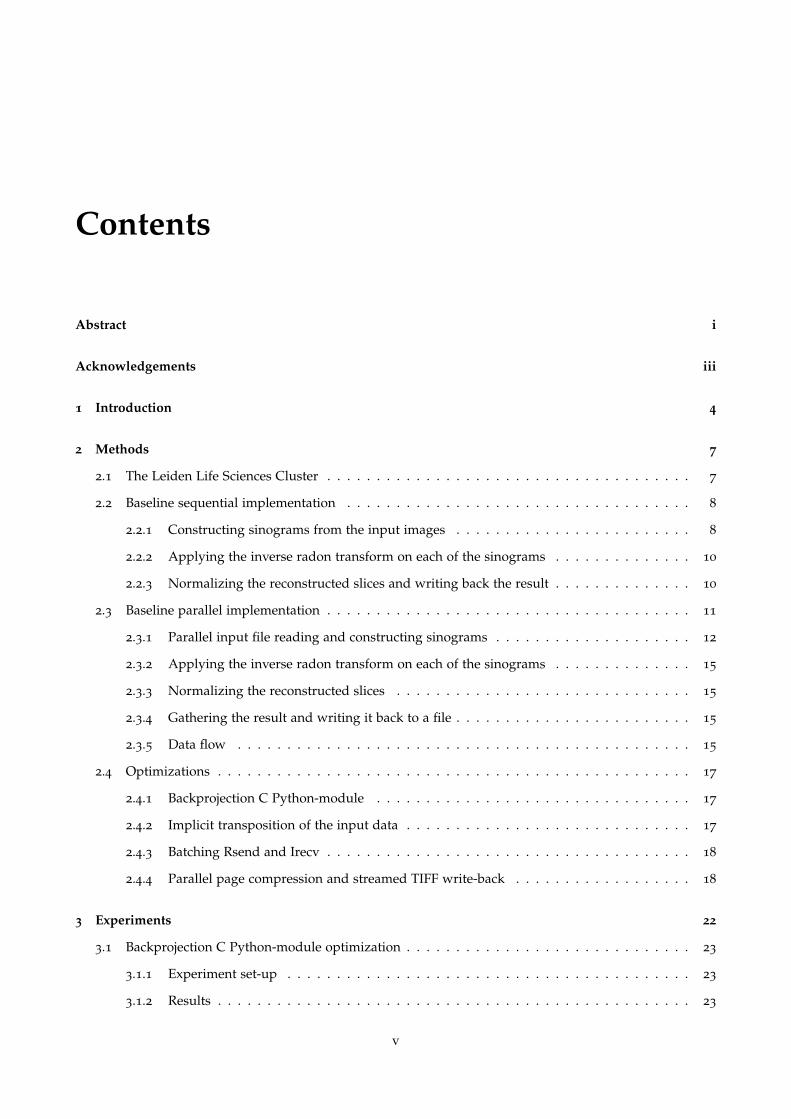
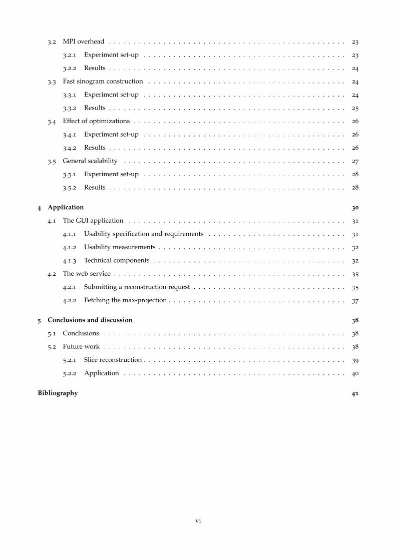
Contents

Abstract i

Acknowledgements iii

1 Introduction 4

2 Methods 7

2.1 The Leiden Life Sciences Cluster . . . . . . . . . . . . . . . . . . . . . . . . . . . . . . . . . . . . . 7

2.2 Baseline sequential implementation . . . . . . . . . . . . . . . . . . . . . . . . . . . . . . . . . . . 8

2.2.1 Constructing sinograms from the input images . . . . . . . . . . . . . . . . . . . . . . . . 8

2.2.2 Applying the inverse radon transform on each of the sinograms . . . . . . . . . . . . . . 10

2.2.3 Normalizing the reconstructed slices and writing back the result . . . . . . . . . . . . . . 10

2.3 Baseline parallel implementation . . . . . . . . . . . . . . . . . . . . . . . . . . . . . . . . . . . . . 11

2.3.1 Parallel input file reading and constructing sinograms . . . . . . . . . . . . . . . . . . . . 12

2.3.2 Applying the inverse radon transform on each of the sinograms . . . . . . . . . . . . . . 15

2.3.3 Normalizing the reconstructed slices . . . . . . . . . . . . . . . . . . . . . . . . . . . . . . 15

2.3.4 Gathering the result and writing it back to a file . . . . . . . . . . . . . . . . . . . . . . . . 15

2.3.5 Data flow . . . . . . . . . . . . . . . . . . . . . . . . . . . . . . . . . . . . . . . . . . . . . . 15

2.4 Optimizations . . . . . . . . . . . . . . . . . . . . . . . . . . . . . . . . . . . . . . . . . . . . . . . . 17

2.4.1 Backprojection C Python-module . . . . . . . . . . . . . . . . . . . . . . . . . . . . . . . . 17

2.4.2 Implicit transposition of the input data . . . . . . . . . . . . . . . . . . . . . . . . . . . . . 17

2.4.3 Batching Rsend and Irecv . . . . . . . . . . . . . . . . . . . . . . . . . . . . . . . . . . . . . 18

2.4.4 Parallel page compression and streamed TIFF write-back . . . . . . . . . . . . . . . . . . 18

3 Experiments 22

3.1 Backprojection C Python-module optimization . . . . . . . . . . . . . . . . . . . . . . . . . . . . . 23

3.1.1 Experiment set-up . . . . . . . . . . . . . . . . . . . . . . . . . . . . . . . . . . . . . . . . . 23

3.1.2 Results . . . . . . . . . . . . . . . . . . . . . . . . . . . . . . . . . . . . . . . . . . . . . . . . 23

v

3.2 MPI overhead . . . . . . . . . . . . . . . . . . . . . . . . . . . . . . . . . . . . . . . . . . . . . . . . 23


3.2.2 Results . . . . . . . . . . . . . . . . . . . . . . . . . . . . . . . . . . . . . . . . . . . . . . . . 24

3.3 Fast sinogram construction . . . . . . . . . . . . . . . . . . . . . . . . . . . . . . . . . . . . . . . . 24


3.3.2 Results . . . . . . . . . . . . . . . . . . . . . . . . . . . . . . . . . . . . . . . . . . . . . . . . 25

3.4 Effect of optimizations . . . . . . . . . . . . . . . . . . . . . . . . . . . . . . . . . . . . . . . . . . . 26


3.4.2 Results . . . . . . . . . . . . . . . . . . . . . . . . . . . . . . . . . . . . . . . . . . . . . . . . 26

3.5 General scalability . . . . . . . . . . . . . . . . . . . . . . . . . . . . . . . . . . . . . . . . . . . . . 27


3.5.2 Results . . . . . . . . . . . . . . . . . . . . . . . . . . . . . . . . . . . . . . . . . . . . . . . . 28

4 Application 30

4.1 The GUI application . . . . . . . . . . . . . . . . . . . . . . . . . . . . . . . . . . . . . . . . . . . . 31

4.1.1 Usability specification and requirements . . . . . . . . . . . . . . . . . . . . . . . . . . . . 31

4.1.2 Usability measurements . . . . . . . . . . . . . . . . . . . . . . . . . . . . . . . . . . . . . . 32

4.1.3 Technical components . . . . . . . . . . . . . . . . . . . . . . . . . . . . . . . . . . . . . . . 32

4.2 The web service . . . . . . . . . . . . . . . . . . . . . . . . . . . . . . . . . . . . . . . . . . . . . . . 35

4.2.1 Submitting a reconstruction request . . . . . . . . . . . . . . . . . . . . . . . . . . . . . . . 35

4.2.2 Fetching the max-projection . . . . . . . . . . . . . . . . . . . . . . . . . . . . . . . . . . . . 37

5 Conclusions and discussion 38

5.1 Conclusions . . . . . . . . . . . . . . . . . . . . . . . . . . . . . . . . . . . . . . . . . . . . . . . . . 38

5.2 Future work . . . . . . . . . . . . . . . . . . . . . . . . . . . . . . . . . . . . . . . . . . . . . . . . . 38

5.2.1 Slice reconstruction . . . . . . . . . . . . . . . . . . . . . . . . . . . . . . . . . . . . . . . . . 39

5.2.2 Application . . . . . . . . . . . . . . . . . . . . . . . . . . . . . . . . . . . . . . . . . . . . . 40

Bibliography 41

vi

List of Tables

3.1 Performance measurement results of the custom backprojection module. . . . . . . . . . . . . . 23

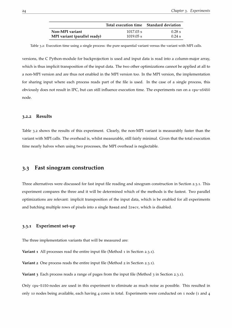
3.2 Execution time using a single process: the pure sequential variant versus the variant with MPI

calls. . . . . . . . . . . . . . . . . . . . . . . . . . . . . . . . . . . . . . . . . . . . . . . . . . . . . . 24

3.3 Performance comparision between the three tested methods to construct a range of sinograms

in each process’s memory. . . . . . . . . . . . . . . . . . . . . . . . . . . . . . . . . . . . . . . . . . 25

3.4 Performance comparision of different kinds of optimizations. . . . . . . . . . . . . . . . . . . . . 26

3.5 Effect of different processor and node counts on the total execution speed. . . . . . . . . . . . . 29

1

List of Figures

1.1 Overview of different small-scale imaging modalities and the range of resolution it can be

applied in [KBK+09]. Both OPT and CLSM are part of light microscopy. . . . . . . . . . . . . . . 4

1.2 OPT image aquisition: OPT imagine system and OPT images generated by it. . . . . . . . . . . 5

1.3 Slice-based OPT image reconstruction. . . . . . . . . . . . . . . . . . . . . . . . . . . . . . . . . . . 5

1.4 3D visualization of a zebrafish produced by Amira [FEI]. Two channels are visualized: a

brightfield channel visualizing the zebrafish itself and a fluorecent channel, highlighting points

of interest. . . . . . . . . . . . . . . . . . . . . . . . . . . . . . . . . . . . . . . . . . . . . . . . . . . 6

2.1 Constructing sinograms from input OPT images and reconstruction of slices. . . . . . . . . . . . 9

2.2 3D visualization of the relation between OPT images and sinograms. Each cube represents a

pixel. . . . . . . . . . . . . . . . . . . . . . . . . . . . . . . . . . . . . . . . . . . . . . . . . . . . . . 9

2.3 Transposition of the input image. . . . . . . . . . . . . . . . . . . . . . . . . . . . . . . . . . . . . . 10

2.4 The different kinds of data the input image is pulled through. Dimensions of typical input

data are listed as well and the datatype of each pixel. . . . . . . . . . . . . . . . . . . . . . . . . . 11

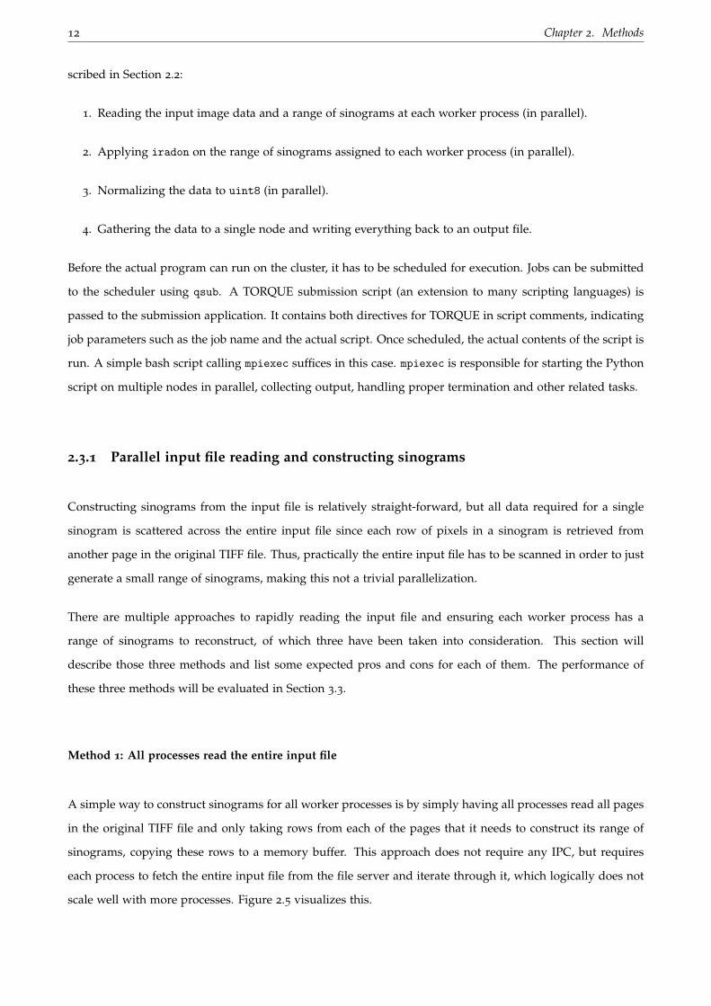
2.5 An example with two processes: all processes read the entire input file and copy required rows

of pixels to their local sinogram array. No IPC is needed. . . . . . . . . . . . . . . . . . . . . . . . 13

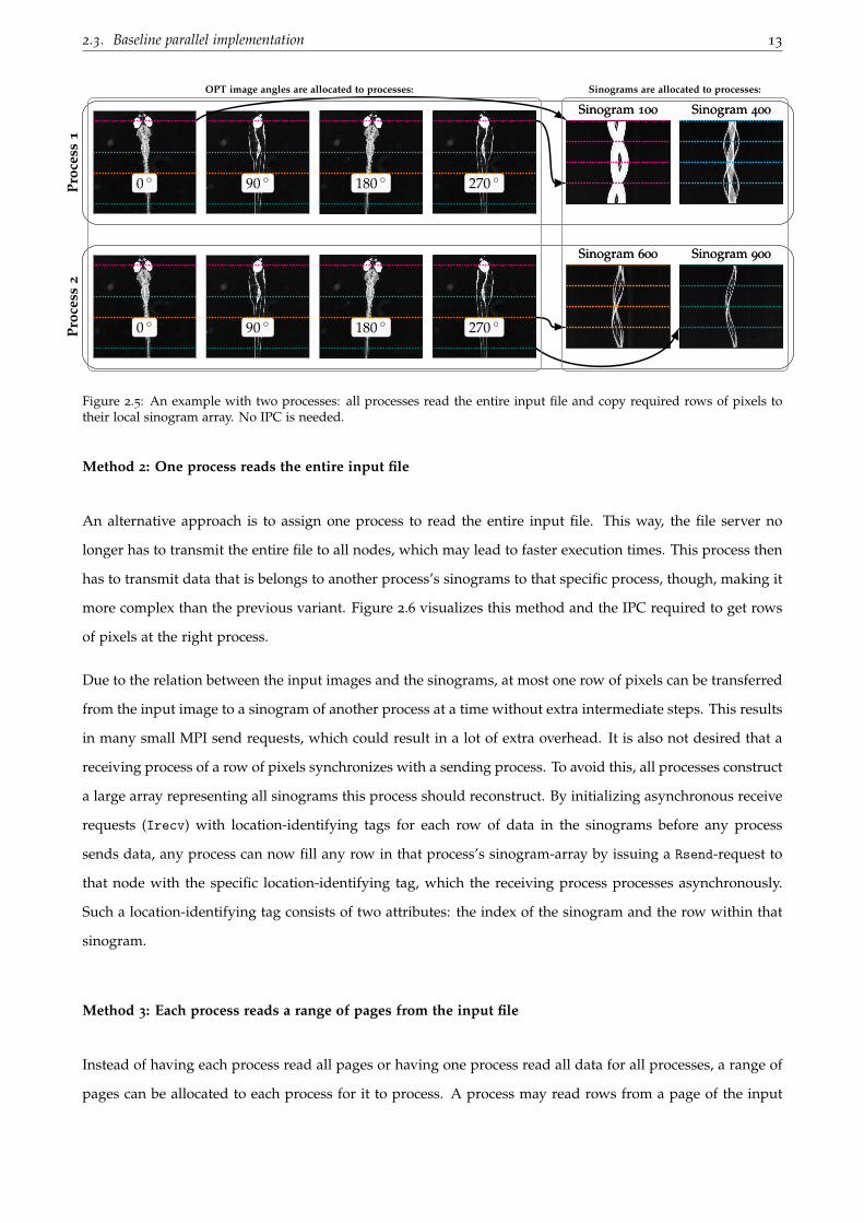
2.6 An example with two processes: the first process reads the entire input file. IPC is used to

transfer rows of pixels to other processes when needed. . . . . . . . . . . . . . . . . . . . . . . . 14

2.7 An example with two processes: each process has a range of sinograms it has to reconstruct

and each process reads a range of pages from the input file. . . . . . . . . . . . . . . . . . . . . . 14

2.8 Full data flow diagram using the third sinogram construction method described in Section 2.3.1. 16

2.9 Output file structure with parallel compression and streamed TIFF write-back. . . . . . . . . . . 21

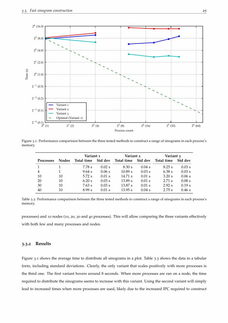
3.1 Performance comparision between the three tested methods to construct a range of sinograms

in each process’s memory. . . . . . . . . . . . . . . . . . . . . . . . . . . . . . . . . . . . . . . . . . 25

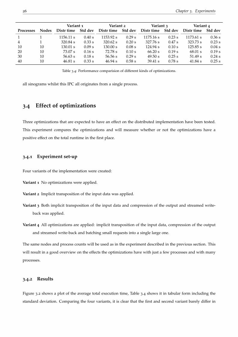
3.2 Performance comparision of different kinds of optimizations. . . . . . . . . . . . . . . . . . . . . 27

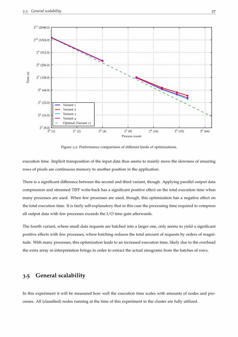
3.3 Effect of different processor and node counts on the total execution speed. . . . . . . . . . . . . 28

2

LIST OF FIGURES 3

4.1 Original situation requiring manual file transfers and two people. . . . . . . . . . . . . . . . . . 30

4.2 Desired situation with an intermediate application uploading the data to the LLSC. . . . . . . . 31

4.3 Screenshot of the prototype GUI application once reconstruction has finished. . . . . . . . . . . 33

4.4 Screenshot of the prototype GUI application during upload. . . . . . . . . . . . . . . . . . . . . . 33

4.5 Max-projection from a stack of reconstructed slices. . . . . . . . . . . . . . . . . . . . . . . . . . . 36

Chapter 1

Introduction

Optical projection tomography (OPT) is a form of tomography involving optical microscopy [Sha04]. It uses

visible light to image small animals, organs or embryos. In microbiology, green fluorescent protein (GFP) is

frequently used as a tracer molecule by first inserting the gene for constructing GFP in the gene for a protein.

This causes the cell to produce GFP whenever the protein is produced, attached to the protein. Under UV

light, these GFP molecules emit green light and this can be used to determine where the protein is located.

OPT is one way to image this in 3D.

Confocal laser scanning microscopy (CLSM) is an alternative imaging method to construct 3D images using

visible light. CLSM has the disadvantage that the light rays cannot reach deep enough in the specimen. With

CLSM, the specimen can be sectioned in in several thin layers and the different CLSM results can be stitched

together in order to construct a larger 3D image. OPT has the advantage that it allows larger specimens to

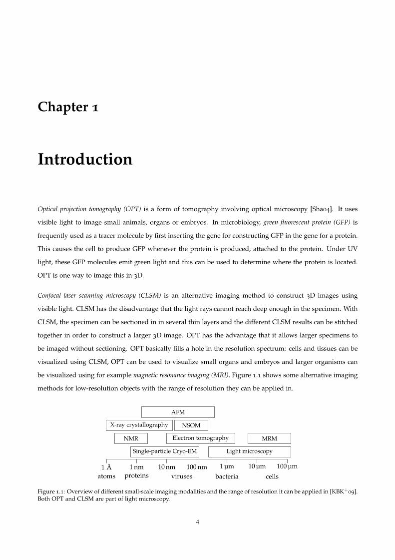
be imaged without sectioning. OPT basically fills a hole in the resolution spectrum: cells and tissues can be

visualized using CLSM, OPT can be used to visualize small organs and embryos and larger organisms can

be visualized using for example magnetic resonance imaging (MRI). Figure 1.1 shows some alternative imaging

methods for low-resolution objects with the range of resolution they can be applied in.

1 A 100 µm10 µm1 µm100 nm10 nm1 nm

atoms proteins viruses bacteria cells

Single-particle Cryo-EM

NMR

X-ray crystallography

AFM

NSOM

Electron tomography

Light microscopy

MRM

Figure 1.1: Overview of different small-scale imaging modalities and the range of resolution it can be applied in [KBK+09].Both OPT and CLSM are part of light microscopy.

4

5

OPT imaging system OPT images(400 images/angles)

0 ◦ 90 ◦

180 ◦ 270 ◦

generates

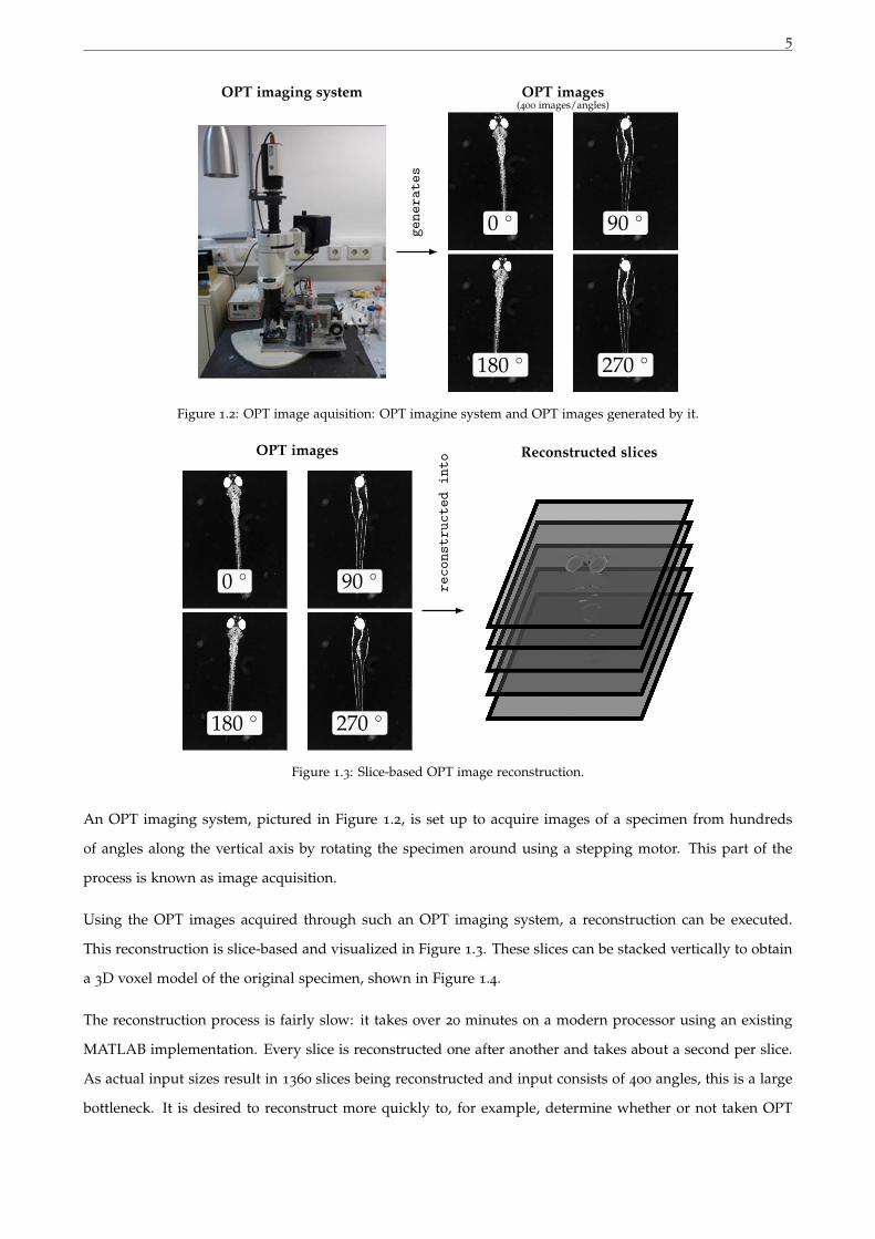
Figure 1.2: OPT image aquisition: OPT imagine system and OPT images generated by it.

OPT images Reconstructed slices

0 ◦ 90 ◦

180 ◦ 270 ◦

reconstructedinto

Figure 1.3: Slice-based OPT image reconstruction.

An OPT imaging system, pictured in Figure 1.2, is set up to acquire images of a specimen from hundreds

of angles along the vertical axis by rotating the specimen around using a stepping motor. This part of the

process is known as image acquisition.

Using the OPT images acquired through such an OPT imaging system, a reconstruction can be executed.

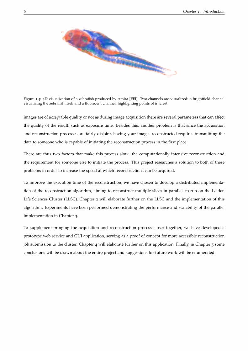
This reconstruction is slice-based and visualized in Figure 1.3. These slices can be stacked vertically to obtain

a 3D voxel model of the original specimen, shown in Figure 1.4.

The reconstruction process is fairly slow: it takes over 20 minutes on a modern processor using an existing

MATLAB implementation. Every slice is reconstructed one after another and takes about a second per slice.

As actual input sizes result in 1360 slices being reconstructed and input consists of 400 angles, this is a large

bottleneck. It is desired to reconstruct more quickly to, for example, determine whether or not taken OPT

6 Chapter 1. Introduction

Figure 1.4: 3D visualization of a zebrafish produced by Amira [FEI]. Two channels are visualized: a brightfield channelvisualizing the zebrafish itself and a fluorecent channel, highlighting points of interest.

images are of acceptable quality or not as during image acquisition there are several parameters that can affect

the quality of the result, such as exposure time. Besides this, another problem is that since the acquisition

and reconstruction processes are fairly disjoint, having your images reconstructed requires transmitting the

data to someone who is capable of initiating the reconstruction process in the first place.

There are thus two factors that make this process slow: the computationally intensive reconstruction and

the requirement for someone else to initiate the process. This project researches a solution to both of these

problems in order to increase the speed at which reconstructions can be acquired.

To improve the execution time of the reconstruction, we have chosen to develop a distributed implementa-

tion of the reconstruction algorithm, aiming to reconstruct multiple slices in parallel, to run on the Leiden

Life Sciences Cluster (LLSC). Chapter 2 will elaborate further on the LLSC and the implementation of this

algorithm. Experiments have been performed demonstrating the performance and scalability of the parallel

implementation in Chapter 3.

To supplement bringing the acquisition and reconstruction process closer together, we have developed a

prototype web service and GUI application, serving as a proof of concept for more accessible reconstruction

job submission to the cluster. Chapter 4 will elaborate further on this application. Finally, in Chapter 5 some

conclusions will be drawn about the entire project and suggestions for future work will be enumerated.

Chapter 2

Methods

This chapter will cover the approach to the problem, what hardware and software was used for the imple-

mentation and the optimizations applied to the baseline distributed implementation.

2.1 The Leiden Life Sciences Cluster

The Leiden Life Sciences Cluster (LLSC) is used to run the software. It is a cluster consisting of three user nodes,

a range of compute nodes and a file server. The Maui scheduler is used to schedule the submitted jobs to the

cluster on the user node together with the TORQUE resource manager.

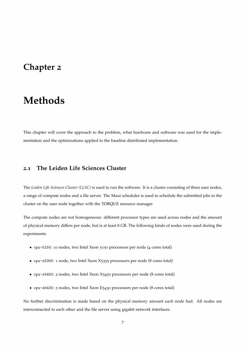
The compute nodes are not homogeneous: different processor types are used across nodes and the amount

of physical memory differs per node, but is at least 8 GB. The following kinds of nodes were used during the

experiments:

• cpu-5150: 10 nodes, two Intel Xeon 5150 processors per node (4 cores total)

• cpu-x5355: 1 node, two Intel Xeon X5355 processors per node (8 cores total)

• cpu-x5450: 2 nodes, two Intel Xeon X5450 processors per node (8 cores total)

• cpu-e5430: 5 nodes, two Intel Xeon E5430 processors per node (8 cores total)

No further discrimination is made based on the physical memory amount each node had. All nodes are

interconnected to each other and the file server using gigabit network interfaces.

7

8 Chapter 2. Methods

2.2 Baseline sequential implementation

A simple implementation of the entire algorithm to reconstruct slices from OPT input images already existed

in MATLAB [Tan16]. The baseline sequential implementation is a fairly straight-forward conversion of this

MATLAB code to Python code, utilizing several libraries replacing the MATLAB toolboxes used:

• NumPy

• scikit-image (built-in iradon function)

• pillow (reading multipage TIFF files)

• tifffile (writing multipage TIFF files)

Python 2.7 has been chosen to implement everything on. There exist extremely powerful scientific libraries for

Python, such as NumPy. The Python-package scikit-image contains several functions to perform the inverse

radon transform [sidt]. Python 2.7 also runs on the LLSC without any hassle, which is a large advantage.

The entire implementation can be divided into three parts:

1. Reading the input image data into a large NumPy array, then constructing sinograms for each of the

output slices from the input image data

2. Applying the inverse radon transform (iradon) on each of the sinograms, generating reconstructed output

slices.

3. Normalizing the output slices from double to uint8 and writing back the image data to an output file.

2.2.1 Constructing sinograms from the input images

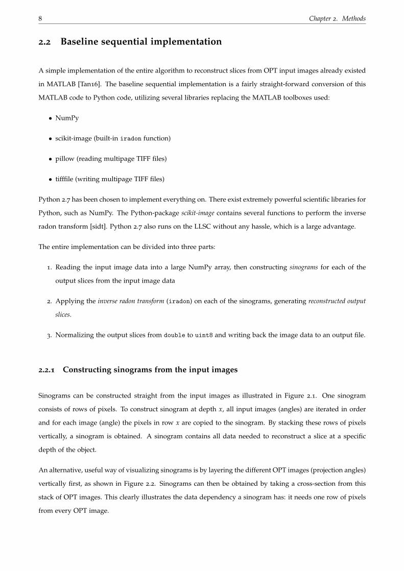
Sinograms can be constructed straight from the input images as illustrated in Figure 2.1. One sinogram

consists of rows of pixels. To construct sinogram at depth x, all input images (angles) are iterated in order

and for each image (angle) the pixels in row x are copied to the sinogram. By stacking these rows of pixels

vertically, a sinogram is obtained. A sinogram contains all data needed to reconstruct a slice at a specific

depth of the object.

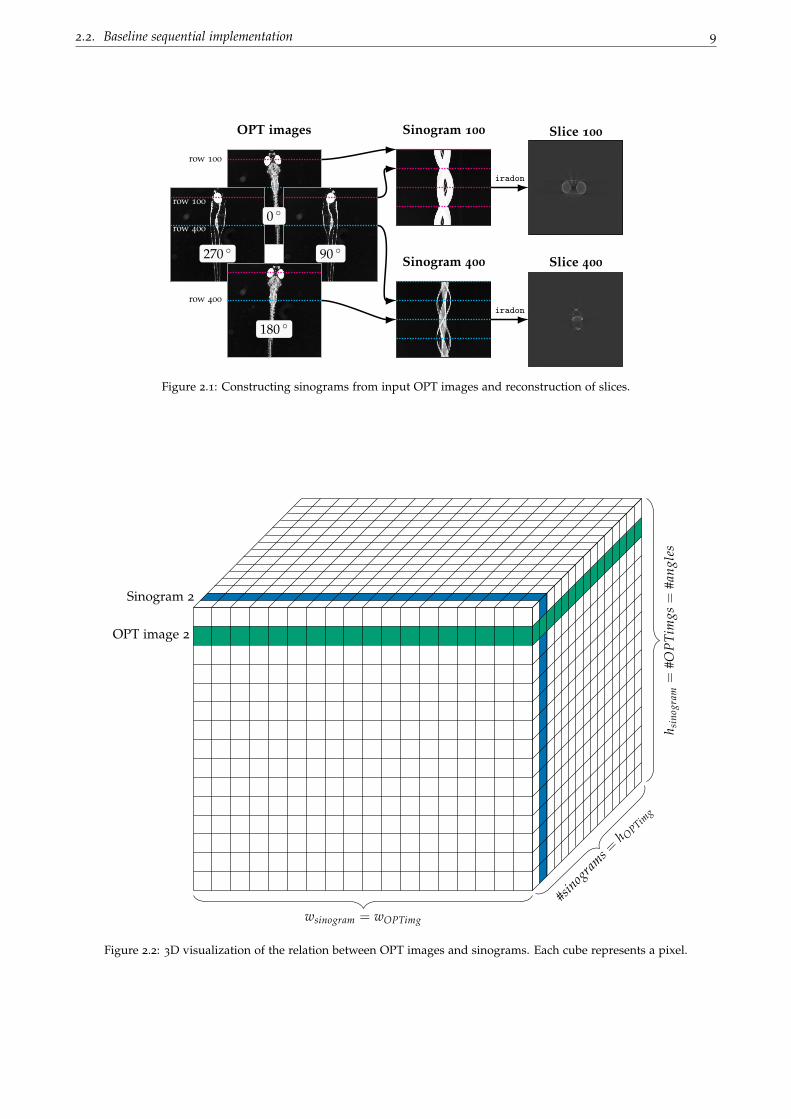
An alternative, useful way of visualizing sinograms is by layering the different OPT images (projection angles)

vertically first, as shown in Figure 2.2. Sinograms can then be obtained by taking a cross-section from this

stack of OPT images. This clearly illustrates the data dependency a sinogram has: it needs one row of pixels

from every OPT image.

2.2. Baseline sequential implementation 9

0 ◦

90 ◦

180 ◦

270 ◦

Sinogram 100OPT images

Sinogram 400 Slice 400

Slice 100

iradon

iradon

row 100

row 400

row 100

row 400

Figure 2.1: Constructing sinograms from input OPT images and reconstruction of slices.

Sinogram 2

OPT image 2

#sin

ogra

ms =

h OPTim

g

hsi

nog

ram=

#OP

Tim

gs=

#an

gle

s

wsinogram = wOPTimg

Figure 2.2: 3D visualization of the relation between OPT images and sinograms. Each cube represents a pixel.


transpose

Original input image data Transposed view

Figure 2.3: Transposition of the input image.

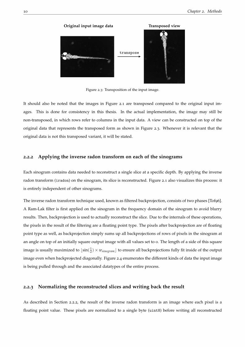
It should also be noted that the images in Figure 2.1 are transposed compared to the original input im-

ages. This is done for consistency in this thesis. In the actual implementation, the image may still be

non-transposed, in which rows refer to columns in the input data. A view can be constructed on top of the

original data that represents the transposed form as shown in Figure 2.3. Whenever it is relevant that the

original data is not this transposed variant, it will be stated.

2.2.2 Applying the inverse radon transform on each of the sinograms

Each sinogram contains data needed to reconstruct a single slice at a specific depth. By applying the inverse

radon transform (iradon) on the sinogram, its slice is reconstructed. Figure 2.1 also visualizes this process: it

is entirely independent of other sinograms.

The inverse radon transform technique used, known as filtered backprojection, consists of two phases [Tof96].

A Ram-Lak filter is first applied on the sinogram in the frequency domain of the sinogram to avoid blurry

results. Then, backprojection is used to actually reconstruct the slice. Due to the internals of these operations,

the pixels in the result of the filtering are a floating point type. The pixels after backprojection are of floating

point type as well, as backprojection simply sums up all backprojections of rows of pixels in the sinogram at

an angle on top of an initially square output image with all values set to 0. The length of a side of this square

image is usually maximized to ⌊sin( 12 )× wsinogram⌋ to ensure all backprojections fully fit inside of the output

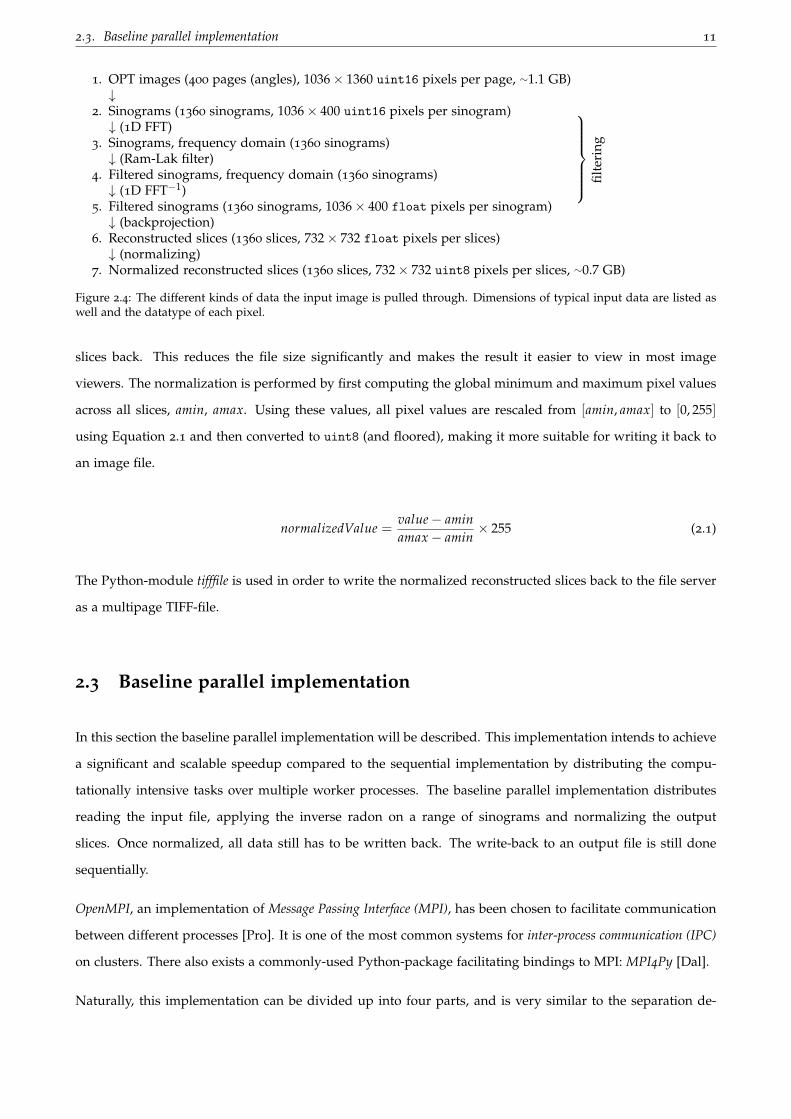
image even when backprojected diagonally. Figure 2.4 enumerates the different kinds of data the input image

is being pulled through and the associated datatypes of the entire process.

2.2.3 Normalizing the reconstructed slices and writing back the result

As described in Section 2.2.2, the result of the inverse radon transform is an image where each pixel is a

floating point value. These pixels are normalized to a single byte (uint8) before writing all reconstructed

2.3. Baseline parallel implementation 11

1. OPT images (400 pages (angles), 1036 × 1360 uint16 pixels per page, ∼1.1 GB)↓

2. Sinograms (1360 sinograms, 1036 × 400 uint16 pixels per sinogram)↓ (1D FFT)

3. Sinograms, frequency domain (1360 sinograms)↓ (Ram-Lak filter)

4. Filtered sinograms, frequency domain (1360 sinograms)

filt

erin

g

↓ (1D FFT−1)5. Filtered sinograms (1360 sinograms, 1036 × 400 float pixels per sinogram)

↓ (backprojection)6. Reconstructed slices (1360 slices, 732 × 732 float pixels per slices)

↓ (normalizing)7. Normalized reconstructed slices (1360 slices, 732 × 732 uint8 pixels per slices, ∼0.7 GB)

Figure 2.4: The different kinds of data the input image is pulled through. Dimensions of typical input data are listed aswell and the datatype of each pixel.

slices back. This reduces the file size significantly and makes the result it easier to view in most image

viewers. The normalization is performed by first computing the global minimum and maximum pixel values

across all slices, amin, amax. Using these values, all pixel values are rescaled from [amin, amax] to [0, 255]

using Equation 2.1 and then converted to uint8 (and floored), making it more suitable for writing it back to

an image file.

normalizedValue =value − amin

amax − amin× 255 (2.1)

The Python-module tifffile is used in order to write the normalized reconstructed slices back to the file server

as a multipage TIFF-file.

2.3 Baseline parallel implementation

In this section the baseline parallel implementation will be described. This implementation intends to achieve

a significant and scalable speedup compared to the sequential implementation by distributing the compu-

tationally intensive tasks over multiple worker processes. The baseline parallel implementation distributes

reading the input file, applying the inverse radon on a range of sinograms and normalizing the output

slices. Once normalized, all data still has to be written back. The write-back to an output file is still done

sequentially.

OpenMPI, an implementation of Message Passing Interface (MPI), has been chosen to facilitate communication

between different processes [Pro]. It is one of the most common systems for inter-process communication (IPC)

on clusters. There also exists a commonly-used Python-package facilitating bindings to MPI: MPI4Py [Dal].

Naturally, this implementation can be divided up into four parts, and is very similar to the separation de-


scribed in Section 2.2:

1. Reading the input image data and a range of sinograms at each worker process (in parallel).

2. Applying iradon on the range of sinograms assigned to each worker process (in parallel).

3. Normalizing the data to uint8 (in parallel).

4. Gathering the data to a single node and writing everything back to an output file.

Before the actual program can run on the cluster, it has to be scheduled for execution. Jobs can be submitted

to the scheduler using qsub. A TORQUE submission script (an extension to many scripting languages) is

passed to the submission application. It contains both directives for TORQUE in script comments, indicating

job parameters such as the job name and the actual script. Once scheduled, the actual contents of the script is

run. A simple bash script calling mpiexec suffices in this case. mpiexec is responsible for starting the Python

script on multiple nodes in parallel, collecting output, handling proper termination and other related tasks.

2.3.1 Parallel input file reading and constructing sinograms

Constructing sinograms from the input file is relatively straight-forward, but all data required for a single

sinogram is scattered across the entire input file since each row of pixels in a sinogram is retrieved from

another page in the original TIFF file. Thus, practically the entire input file has to be scanned in order to just

generate a small range of sinograms, making this not a trivial parallelization.

There are multiple approaches to rapidly reading the input file and ensuring each worker process has a

range of sinograms to reconstruct, of which three have been taken into consideration. This section will

describe those three methods and list some expected pros and cons for each of them. The performance of

these three methods will be evaluated in Section 3.3.

Method 1: All processes read the entire input file

A simple way to construct sinograms for all worker processes is by simply having all processes read all pages

in the original TIFF file and only taking rows from each of the pages that it needs to construct its range of

sinograms, copying these rows to a memory buffer. This approach does not require any IPC, but requires

each process to fetch the entire input file from the file server and iterate through it, which logically does not

scale well with more processes. Figure 2.5 visualizes this.


0 ◦ 90 ◦ 180 ◦ 270 ◦

Sinogram 100 Sinogram 400


0 ◦ 90 ◦ 180 ◦ 270 ◦



Sinograms are allocated to processes:OPT image angles are allocated to processes:

Pro

cess

1P

roce

ss2

Figure 2.5: An example with two processes: all processes read the entire input file and copy required rows of pixels totheir local sinogram array. No IPC is needed.

Method 2: One process reads the entire input file

An alternative approach is to assign one process to read the entire input file. This way, the file server no

longer has to transmit the entire file to all nodes, which may lead to faster execution times. This process then

has to transmit data that is belongs to another process’s sinograms to that specific process, though, making it

more complex than the previous variant. Figure 2.6 visualizes this method and the IPC required to get rows

of pixels at the right process.

Due to the relation between the input images and the sinograms, at most one row of pixels can be transferred

from the input image to a sinogram of another process at a time without extra intermediate steps. This results

in many small MPI send requests, which could result in a lot of extra overhead. It is also not desired that a

receiving process of a row of pixels synchronizes with a sending process. To avoid this, all processes construct

a large array representing all sinograms this process should reconstruct. By initializing asynchronous receive

requests (Irecv) with location-identifying tags for each row of data in the sinograms before any process

sends data, any process can now fill any row in that process’s sinogram-array by issuing a Rsend-request to

that node with the specific location-identifying tag, which the receiving process processes asynchronously.

Such a location-identifying tag consists of two attributes: the index of the sinogram and the row within that

sinogram.

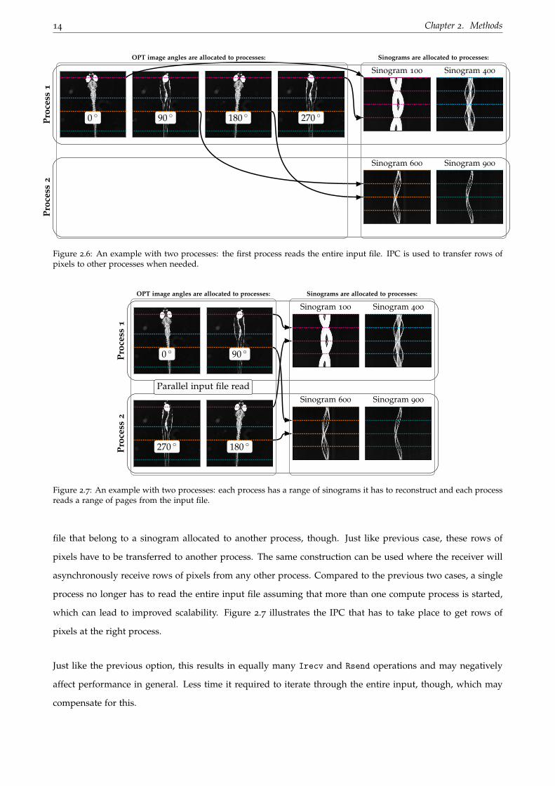
Method 3: Each process reads a range of pages from the input file

Instead of having each process read all pages or having one process read all data for all processes, a range of

pages can be allocated to each process for it to process. A process may read rows from a page of the input


0 ◦ 90 ◦ 180 ◦ 270 ◦




Pro

cess

1P

roce

ss2

Figure 2.6: An example with two processes: the first process reads the entire input file. IPC is used to transfer rows ofpixels to other processes when needed.

0 ◦ 90 ◦

180 ◦270 ◦




Pro

cess

1P

roce

ss2

Parallel input file read

Figure 2.7: An example with two processes: each process has a range of sinograms it has to reconstruct and each processreads a range of pages from the input file.

file that belong to a sinogram allocated to another process, though. Just like previous case, these rows of

pixels have to be transferred to another process. The same construction can be used where the receiver will

asynchronously receive rows of pixels from any other process. Compared to the previous two cases, a single

process no longer has to read the entire input file assuming that more than one compute process is started,

which can lead to improved scalability. Figure 2.7 illustrates the IPC that has to take place to get rows of

pixels at the right process.

Just like the previous option, this results in equally many Irecv and Rsend operations and may negatively

affect performance in general. Less time it required to iterate through the entire input, though, which may

compensate for this.


2.3.2 Applying the inverse radon transform on each of the sinograms

Once the input file has been transformed into sinograms and each compute process now has a range of sino-

grams in its memory, each process can reconstruct the assigned sinograms using the inverse radon transform.

This works exactly the same as the method described in Section 2.2.2, but since each process has a small

subset of all sinograms assigned, it executes a lot faster when multiple processes are used.

2.3.3 Normalizing the reconstructed slices

Normalization to uint8 can be performed in parallel too. First, the local minimum and maximum pixel-

values in the reconstructed slices are computed in parallel. Each process computes these values for their own

reconstructed slices. Then, all the local minimum and maximum values are reduced to a global minimum

and maximum value. Once these values are computed, the compute processes can normalize all pixel-values

to uint8 using the technique described in Section 2.2.3.

Note that the reduce operation is blocking and also serves as a synchronization point for all processes. There

is no way any worker process finishes the reduce operation before all processes have started it.

2.3.4 Gathering the result and writing it back to a file

After normalization, the result cannot instantly be written back as the normalized reconstructed slices are

spread across the different worker processes. The result has to be collected to a single master worker process

before writing it back to a file, often referred to as a gather-operation. The master-node is always chosen to

be the last worker process because due to the way sinograms (and thus slices) are allocated to the processes,

the last process has most chance of having fewer sinograms allocated compared to all other process and may

thus enter the gather-stage of the entire process more quickly as it has to normalize fewer slices, reducing the

amount of time other processes have to potentially wait on the master process to be ready.

The master-node preallocates a 3D array in which all reconstructed slices will be placed. MPI has efficient

gather-procedures built-in. Gatherv is used to gather data to the master node. After the gather, the multipage

TIFF output file can be generated from this 3D array using tifffile as described in Section 2.2.3.

2.3.5 Data flow

The concrete actions of the entire process are enumerated in this section. Additionally, this section presents

a data flow diagram illustrating all IPC between different worker processes and file operations with files on


Worker process 1 Worker process 2 Worker process 3 Worker process n

File serverJob script (user node)

. . .

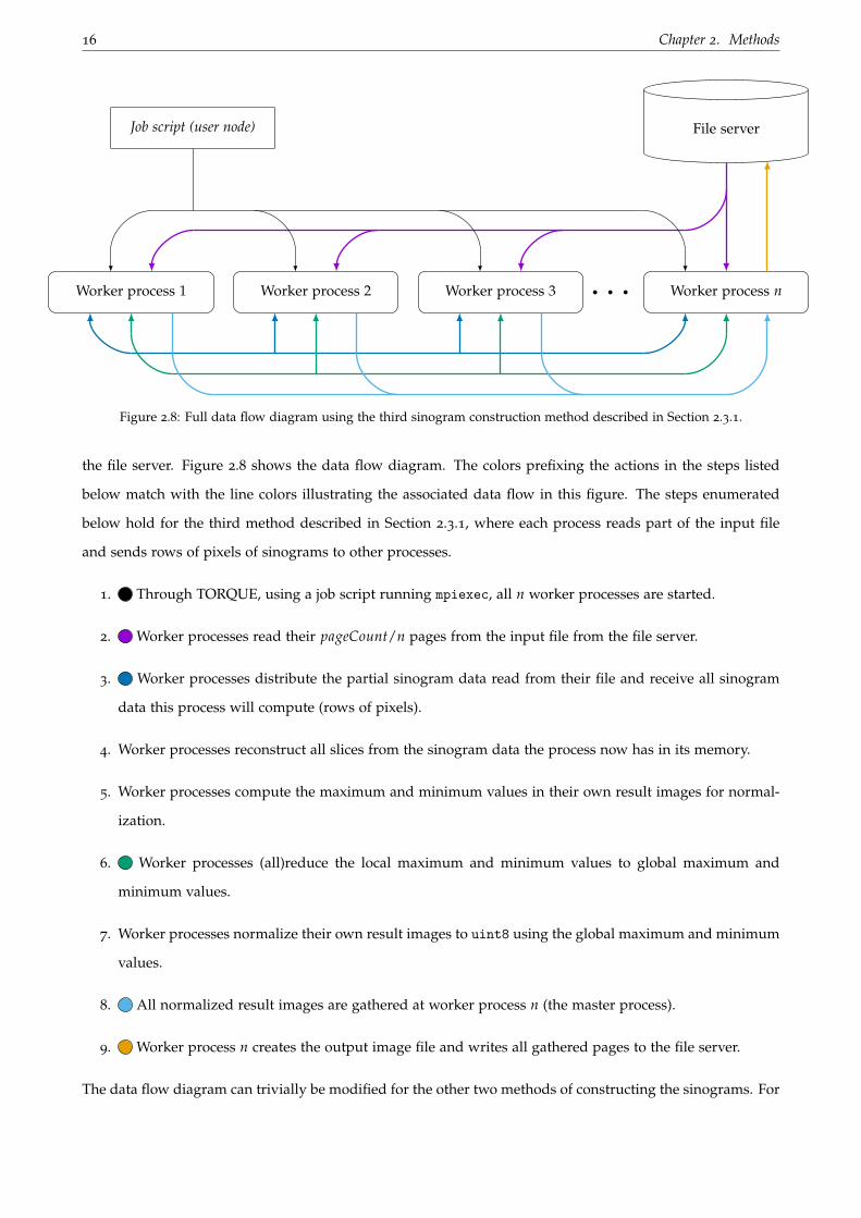
Figure 2.8: Full data flow diagram using the third sinogram construction method described in Section 2.3.1.

the file server. Figure 2.8 shows the data flow diagram. The colors prefixing the actions in the steps listed

below match with the line colors illustrating the associated data flow in this figure. The steps enumerated

below hold for the third method described in Section 2.3.1, where each process reads part of the input file

and sends rows of pixels of sinograms to other processes.

1. Through TORQUE, using a job script running mpiexec, all n worker processes are started.

2. Worker processes read their pageCount/n pages from the input file from the file server.

3. Worker processes distribute the partial sinogram data read from their file and receive all sinogram

data this process will compute (rows of pixels).

4. Worker processes reconstruct all slices from the sinogram data the process now has in its memory.

5. Worker processes compute the maximum and minimum values in their own result images for normal-

ization.

6. Worker processes (all)reduce the local maximum and minimum values to global maximum and

minimum values.

7. Worker processes normalize their own result images to uint8 using the global maximum and minimum

values.

8. All normalized result images are gathered at worker process n (the master process).

9. Worker process n creates the output image file and writes all gathered pages to the file server.

The data flow diagram can trivially be modified for the other two methods of constructing the sinograms. For

2.4. Optimizations 17

the method 1 described in Section 2.3.1, where every worker process reads the entire input file, the -colored

line (and associated step) can be removed. As each process simply derives all data from the entire input file,

no IPC is required for sinogram construction.

For method 2 described in Section 2.3.1, where a single process reads the entire input file but transmits

sinogram data to other processes through IPC, the data flow diagram can be modified by ensuring the -

colored line only goes to one process: the single process that reads the entire input file. IPC is then required

to send sinogram data to other processes. The -colored line represents this communication and should thus

always start at the process reading the entire input file and transmit data to all other worker processes. It will

obviously never receive data.

2.4 Optimizations

In Section 2.3 the baseline implementation has been described. This implementation can make use of multiple

of the LLSC’s compute nodes to reconstruct the slices in parallel. In order to speed up execution time more,

a number of optimizations have been applied to this implementation, which are described in this section.

2.4.1 Backprojection C Python-module

The inverse radon transform consists of two phases: a ramp filter and the actual backprojection. The scikit-

image implementation was originally used for both of these operations. Whilst the first phase is relatively

fast, the second phase is extremely slow due to many large array operations.

To improve the performance, a Python-module written in C has been developed for faster backprojection.

The algorithm used within this Python-module is heavily based upon the code used in an existing module

for MATLAB [Orc06]. This module iterates the memory of the output image in sequential order, speeding up

memory access speeds, avoids unpredictable branches and does not allocate memory in the algorithm’s hot

loops.

2.4.2 Implicit transposition of the input data

In the original input data, the image is rotated in a way such that the lines of pixels that need to be copied into

sinograms are not continuous memory, assuming the default row-major arrays are used, as shown in Figure

2.3. This requires copying each line of pixels, which are in fact columns of pixels in the original image, into a

temporary buffer before it can be sent using a MPI message. This can cause a lot of extra overhead. NumPy


supports both row-major and column-major arrays. By reading the input images into a column-major order

array, single rows of pixels are continuous memory. Whilst the rows of sinograms are sent from column-major

order arrays, they are still received in a row-major order array (the sinogram array), which has the effect of

implicitly transposing the input image data. Obviously, reading all data into a column-major array is more

expensive than reading it into a row-major array, since the input TIFF images are scanline based (the pixel

data is stored row by row). This is a trade-off which can have either a positive or negative effect on the total

execution time.

2.4.3 Batching Rsend and Irecv

A potential limitation of performance of the sinogram construction process is the large amount of Rsend and

Irecv operations if each process does not fetch all sinogram data on its own. Every single process has to

reconstruct a range of sinograms. From any input image (angle), any process needs multiple rows of pixels

given that it is assigned multiple sinograms to reconstruct. By ensuring these allocated sinograms are a

continuous range, it is possible to batch multiple Rsend and Irecv requests of a rows of pixels to reduce

the amount of messages being passed around. This utilizes that adjacent rows of pixels in an OPT image is

continuous memory, see also Figure 2.2, assuming that the previous optimization is also applied.

It is important to note that with this optimization it is no longer possible to directly Irecv into the sinogram

array of the compute process, as multiple rows of pixels being received at once belong to different sinograms

and is thus not continuous memory in the receiving process’s sinogram array. It is however still possible to

transform this kind of input to an array of sinograms after all data has been received without any extra IPC

using array re-interpretation, by layering the sequences of rows of sinogram pixels on top of each other, then

taking cross-sections of this stack. This is practically the same as visualized in Figure 2.2, but the depth axis

is now only #assignedSinograms deep rather than the total amount of existing sinograms.

2.4.4 Parallel page compression and streamed TIFF write-back

Compression reduces the total amount of the data being transmitted between nodes and the file server.

Handling data as soon as it arrives instead of a formal gather can improve execution time more as well, as it

avoids blocking for an unnecessary long time on the master process even though this master process can do

work with partial data. This section describes this optimization in detail.


Compression

In the baseline implementation, after parallel normalization, all data is gathered to a single node, which

then writes all data back to a file on the file server at once. Both the gather and write-back are significantly

limited in execution speed by I/O times. The TIFF file format supports per page deflate compression. By

compressing the normalized page data in parallel on all compute nodes the page data can be compressed

quickly. Typically, after compression, the page size is reduced to about 40% of the original output data

size. Thanks to compression, the gather and write-back thus get a significant speedup as less data has to be

transferred from compute nodes to the master compute node and from the master compute node to the file

server.

Streamed TIFF write-back

To improve the gather and write-back times even more, some sort of streamed write-back has been imple-

mented. Typically, the gather operation blocks until all data has been gathered to the master node, after

which the master node will write all gathered data back at once. This gather operation has been replaced by

a mechanism that allows compute nodes to asynchronously ”push” TIFF-compatible1 compressed data to the

master node. The master node simply waits for any data to arrive, then immediately writes the compressed

data to the output file. Once the master has received all data, it will write back some final metadata and

filling in some gaps describing where the compressed page data can be found.

Pushing data to the master node utilizes a similar technique to what is described in the second method in

Section 2.3.1. The master process initializes a large 2D array. One dimension is used to index the slice index

(which is equal to the output TIFF page index), whilst the other is used to contain the compressed data that

should be saved. The master initializes, for each page, an asynchronous receive request using Irecv. To

ensure this buffer is ready for receiving before any other process starts sending compressed data to avoid

blocking worker processes for a long time, this is initialized before the normalization procedure (Section 2.3.3)

starts. Since the normalization procedure contains a synchronization point between all worker processes, it

is guaranteed that this buffer is initialized before any process sends data.

Due to compression, the page data size may vary between pages. The buffer the master initializes must be

large enough to receive any length of compressed data. It must also be possible to recover the original length

of the data once the master receives the data. Other TIFF field values, such as the original image dimensions,

are constructed at the worker processes in parallel too and must be transmitted to the master process. This

data is all packed using a simple binary format that allows recovery of the original data on the receivers end.

1Before page data is written to a TIFF file, it is transformed slightly, which is an operation that has been moved to the compute nodestoo.


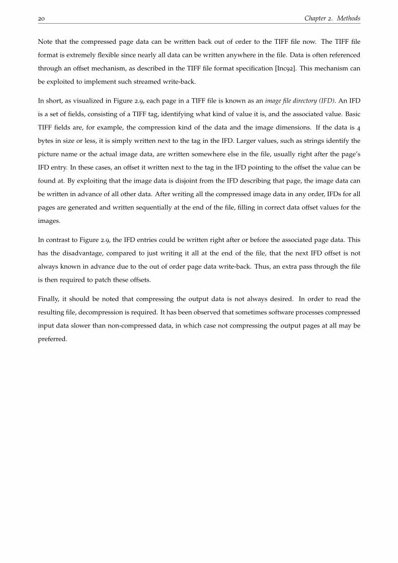
Note that the compressed page data can be written back out of order to the TIFF file now. The TIFF file

format is extremely flexible since nearly all data can be written anywhere in the file. Data is often referenced

through an offset mechanism, as described in the TIFF file format specification [Inc92]. This mechanism can

be exploited to implement such streamed write-back.

In short, as visualized in Figure 2.9, each page in a TIFF file is known as an image file directory (IFD). An IFD

is a set of fields, consisting of a TIFF tag, identifying what kind of value it is, and the associated value. Basic

TIFF fields are, for example, the compression kind of the data and the image dimensions. If the data is 4

bytes in size or less, it is simply written next to the tag in the IFD. Larger values, such as strings identify the

picture name or the actual image data, are written somewhere else in the file, usually right after the page’s

IFD entry. In these cases, an offset it written next to the tag in the IFD pointing to the offset the value can be

found at. By exploiting that the image data is disjoint from the IFD describing that page, the image data can

be written in advance of all other data. After writing all the compressed image data in any order, IFDs for all

pages are generated and written sequentially at the end of the file, filling in correct data offset values for the

images.

In contrast to Figure 2.9, the IFD entries could be written right after or before the associated page data. This

has the disadvantage, compared to just writing it all at the end of the file, that the next IFD offset is not

always known in advance due to the out of order page data write-back. Thus, an extra pass through the file

is then required to patch these offsets.

Finally, it should be noted that compressing the output data is not always desired. In order to read the

resulting file, decompression is required. It has been observed that sometimes software processes compressed

input data slower than non-compressed data, in which case not compressing the output pages at all may be

preferred.


TIF

Fh

ead

er

Byte order

TIFF marker (42)

1st IFD offset

Page data l

Page data k

Page data 1

Compression field: deflate

Data length field

...

Data offset field

Next IFD offset

Page data m

...

...

Compression field: deflate

Data length field

...

Data offset field

Next IFD offset

Other values (page 1)

...

...

Other values (page m)

...

...

...

1 byte

Len

gth

var

ies

...

...

IFD

1

IFD

2IF

Dm

IFD

m+

1IF

Dn

Next IFD offset = 0

Figure 2.9: Output file structure with parallel compression and streamed TIFF write-back.

Chapter 3

Experiments

A set of experiments have been conducted to determine how well the implementation scales with more

worker processes and what effect the applied optimizations have on the execution time. All experiments were

conducted with warm disk caches by pre-reading the input file twice before running the actual experiment. In

order to obtain more consistent results, runs of the experiments were also conducted after one the other, not

executing multiple runs in parallel. If multiple runs were to execute in parallel, this could result in multiple

jobs doing a lot of I/O at the same time, slowing both runs down significantly. In a practical environment,

these things obviously do not matter. All data points in these experiments were obtained by repeating the

scenario 10 times, removing the best and worst times and then taking the average of the 8 remaining times.

Standard deviations also only use these 8 times.

It should be noted that these experiments were not the only jobs that ran on the cluster. Jobs by other cluster

users ran at the same time as these experiments. Whilst the experiment jobs typically had to wait for these

jobs to finish, it can still have an impact on the execution times as sometimes these jobs did run concurrently.

Two experiments were conducted which did not actually involve parallel execution: measuring the effect of

the backprojection C Python-module optimization and measuring the overhead of MPI with a single process.

Three larger experiments followed that which did involve parallelism: measuring which of the three proposed

ways to read the input file is the fastest and measuring the effect of the different proposed optimizations on

the total execution time. Finally, an experiment is conducted that measures the overall scalability with many

nodes.

22

3.1. Backprojection C Python-module optimization 23

Total execution time Standard deviation

scikit-image backprojection 8764.76 s 12.50 sCustom backprojection 1017.03 s 0.28 s

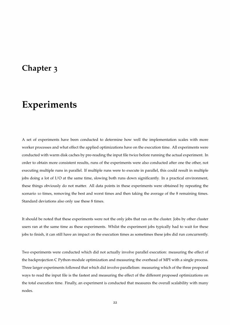
Table 3.1: Performance measurement results of the custom backprojection module.

3.1 Backprojection C Python-module optimization

The primary single-core optimization applied is the backprojection C Python-module to more quickly re-

construct slices, as the original Python version built into scikit-image was deemed too slow. This experiment

measures the effect of the module in the sequential implementation.

3.1.1 Experiment set-up

Two variants were constructed, one with the original scikit-image backprojection and one with the custom

backprojection. Averages and standard deviations of the total executions time are measured. The times were

measured on a cpu-x5450 node.

3.1.2 Results

Table 3.1 shows the results of this experiment. From this table it can be seen that, on a cpu-x5450 node, the

custom backprojection module is about 8.6 times faster than the original Python-based backprojection built

into scikit-image. This module thus has a lot of impact on the total execution speed of the entire program as

a lot of time is spent running the backprojection operation.

3.2 MPI overhead

When using the parallel variant with a single process, MPI calls still occur. For example, gathers from and

to a single process may come with extra overhead compared to the original sequential version. Within this

experiment the difference in execution time between the original, sequential version and the ”parallel-ready”

version (with MPI calls) executing using one process is measured and compared.


Two versions are used: one without MPI calls and one with MPI calls. The total execution time is measured

from the point the files are being opened until the point the output file has been written back. In both

24 Chapter 3. Experiments

Total execution time Standard deviation

Non-MPI variant 1017.03 s 0.28 sMPI variant (parallel ready) 1019.05 s 0.24 s

Table 3.2: Execution time using a single process: the pure sequential variant versus the variant with MPI calls.

versions, the C Python-module for backprojection is used and input data is read into a column-major array,

which is thus implicit transposition of the input data. The two other optimizations cannot be applied at all to

a non-MPI version and are thus not enabled in the MPI version too. In the MPI version, the implementation

for sharing input where each process reads part of the file is used. In the case of a single process, this

obviously does not result in IPC, but can still influence execution time. The experiments ran on a cpu-x5450

node.

3.2.2 Results

Table 3.2 shows the results of this experiment. Clearly, the non-MPI variant is measurably faster than the

variant with MPI calls. The overhead is, whilst measurable, still fairly minimal. Given that the total execution

time nearly halves when using two processes, the MPI overhead is neglectable.

3.3 Fast sinogram construction

Three alternatives were discussed for fast input file reading and sinogram construction in Section 2.3.1. This

experiment compares the three and it will be determined which of the methods is the fastest. Two parallel

optimizations are relevant: implicit transposition of the input data, which is be enabled for all experiments

and batching multiple rows of pixels into a single Rsend and Irecv, which is disabled.


The three implementation variants that will be measured are:

Variant 1 All processes read the entire input file (Method 1 in Section 2.3.1).

Variant 2 One process reads the entire input file (Method 2 in Section 2.3.1).

Variant 3 Each process reads a range of pages from the input file (Method 3 in Section 2.3.1).

Only cpu-5150-nodes are used in this experiment to eliminate as much noise as possible. This resulted in

only 10 nodes being available, each having 4 cores in total. Experiments were conducted on 1 node (1 and 4

3.3. Fast sinogram construction 25

20 (1) 21 (2) 22 (4) 23 (8) 24 (16) 25 (32) 26 (64)

Process count

2−4 (0.1)

2−3 (0.1)

2−2 (0.2)

2−1 (0.5)

20 (1.0)

21 (2.0)

22 (4.0)

23 (8.0)

24 (16.0)T

ime

(s)

Variant 1

Variant 2

Variant 3

Optimal (Variant 1)

Figure 3.1: Performance comparision between the three tested methods to construct a range of sinograms in each process’smemory.

Variant 1 Variant 2 Variant 3

Processes Nodes Total time Std dev Total time Std dev Total time Std dev

1 1 7.78 s 0.02 s 8.30 s 0.04 s 8.25 s 0.03 s4 1 9.64 s 0.06 s 10.89 s 0.03 s 6.38 s 0.03 s10 10 5.72 s 0.01 s 14.71 s 0.01 s 3.20 s 0.06 s20 10 6.20 s 0.03 s 13.89 s 0.01 s 2.71 s 0.08 s30 10 7.63 s 0.03 s 13.87 s 0.01 s 2.92 s 0.19 s40 10 8.99 s 0.01 s 13.95 s 0.04 s 2.75 s 0.46 s

Table 3.3: Performance comparision between the three tested methods to construct a range of sinograms in each process’smemory.

processes) and 10 nodes (10, 20, 30 and 40 processes). This will allow comparing the three variants effectively

with both few and many processes and nodes.

3.3.2 Results

Figure 3.1 shows the average time to distribute all sinograms in a plot. Table 3.3 shows the data in a tabular

form, including standard deviations. Clearly, the only variant that scales positively with more processes is

the third one. The first variant hovers around 8 seconds. When more processes are ran on a node, the time

required to distribute the sinograms seems to increase with this variant. Using the second variant will simply

lead to increased times when more processes are used, likely due to the increased IPC required to construct


Variant 1 Variant 2 Variant 3 Variant 4

Processes Nodes Distr time Std dev Distr time Std dev Distr time Std dev Distr time Std dev

1 1 1156.11 s 0.40 s 1153.92 s 0.29 s 1175.16 s 0.23 s 1173.61 s 0.36 s4 1 320.84 s 0.33 s 320.62 s 0.20 s 327.76 s 0.47 s 323.73 s 0.23 s10 10 130.01 s 0.09 s 130.00 s 0.08 s 124.94 s 0.10 s 125.85 s 0.04 s20 10 73.07 s 0.16 s 72.78 s 0.10 s 66.20 s 0.19 s 68.01 s 0.19 s30 10 56.63 s 0.18 s 56.56 s 0.29 s 49.50 s 0.25 s 51.49 s 0.24 s40 10 46.81 s 0.33 s 46.94 s 0.58 s 39.41 s 0.78 s 41.84 s 0.25 s

Table 3.4: Performance comparision of different kinds of optimizations.

all sinograms whilst this IPC all originates from a single process.

3.4 Effect of optimizations

Three optimizations that are expected to have an effect on the distributed implementation have been tested.

This experiment compares the optimizations and will measure whether or not the optimizations have a

positive effect on the total runtime in the first place.


Four variants of the implementation were created:

Variant 1 No optimizations were applied.

Variant 2 Implicit transposition of the input data was applied.

Variant 3 Both implicit transposition of the input data and compression of the output and streamed write-

back was applied.

Variant 4 All optimizations are applied: implicit transposition of the input data, compression of the output

and streamed write-back and batching small requests into a single large one.

The same nodes and process counts will be used as in the experiment described in the previous section. This

will result in a good overview on the effects the optimizations have with just a few processes and with many

processes.

3.4.2 Results

Figure 3.2 shows a plot of the average total execution time, Table 3.4 shows it in tabular form including the

standard deviation. Comparing the four variants, it is clear that the first and second variant barely differ in

3.5. General scalability 27

20 (1) 21 (2) 22 (4) 23 (8) 24 (16) 25 (32) 26 (64)

Process count

23 (8.0)

24 (16.0)

25 (32.0)

26 (64.0)

27 (128.0)

28 (256.0)

29 (512.0)

210 (1024.0)

211 (2048.0)T

ime

(s)

Variant 1

Variant 2

Variant 3

Variant 4

Optimal (Variant 1)

Figure 3.2: Performance comparision of different kinds of optimizations.

execution time. Implicit transposition of the input data thus seems to mainly move the slowness of ensuring

rows of pixels are continuous memory to another position in the application.

There is a significant difference between the second and third variant, though. Applying parallel output data

compression and streamed TIFF write-back has a significant positive effect on the total execution time when

many processes are used. When few processes are used, though, this optimization has a negative effect on

the total execution time. It is fairly self-explanatory that in this case the processing time required to compress

all output data with few processes exceeds the I/O time gain afterwards.

The fourth variant, where small data requests are batched into a larger one, only seems to yield a significant

positive effects with few processes, where batching reduces the total amount of requests by orders of magni-

tude. With many processes, this optimization leads to an increased execution time, likely due to the overhead

the extra array re-interpretation brings in order to extract the actual sinograms from the batches of rows.

3.5 General scalability

In this experiment it will be measured how well the execution time scales with amounts of nodes and pro-

cesses. All (classified) nodes running at the time of this experiment in the cluster are fully utilized.


20 (1) 21 (2) 22 (4) 23 (8) 24 (16) 25 (32) 26 (64) 27 (128)

Process count

23 (8.0)

24 (16.0)

25 (32.0)

26 (64.0)

27 (128.0)

28 (256.0)

29 (512.0)

210 (1024.0)

211 (2048.0)T

ime

(s)

1 node

2 nodes

8 nodes

18 nodes

Optimal (Variant 1)

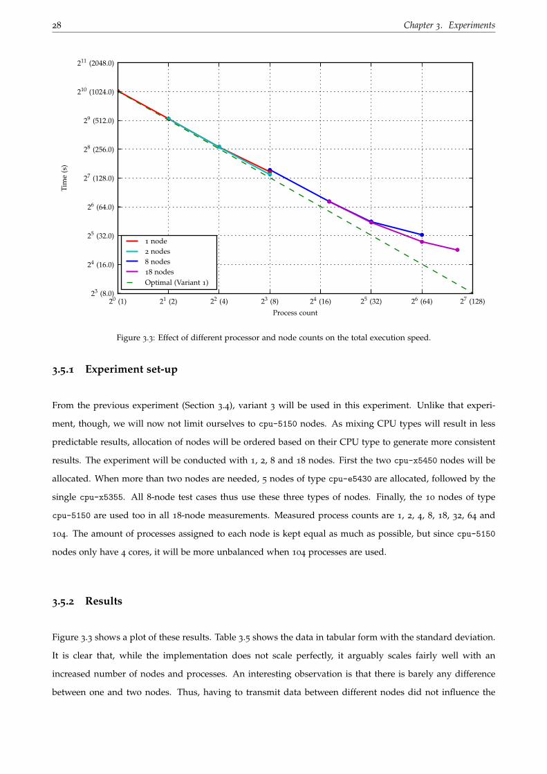
Figure 3.3: Effect of different processor and node counts on the total execution speed.


From the previous experiment (Section 3.4), variant 3 will be used in this experiment. Unlike that experi-

ment, though, we will now not limit ourselves to cpu-5150 nodes. As mixing CPU types will result in less

predictable results, allocation of nodes will be ordered based on their CPU type to generate more consistent

results. The experiment will be conducted with 1, 2, 8 and 18 nodes. First the two cpu-x5450 nodes will be

allocated. When more than two nodes are needed, 5 nodes of type cpu-e5430 are allocated, followed by the

single cpu-x5355. All 8-node test cases thus use these three types of nodes. Finally, the 10 nodes of type

cpu-5150 are used too in all 18-node measurements. Measured process counts are 1, 2, 4, 8, 18, 32, 64 and

104. The amount of processes assigned to each node is kept equal as much as possible, but since cpu-5150

nodes only have 4 cores, it will be more unbalanced when 104 processes are used.

3.5.2 Results

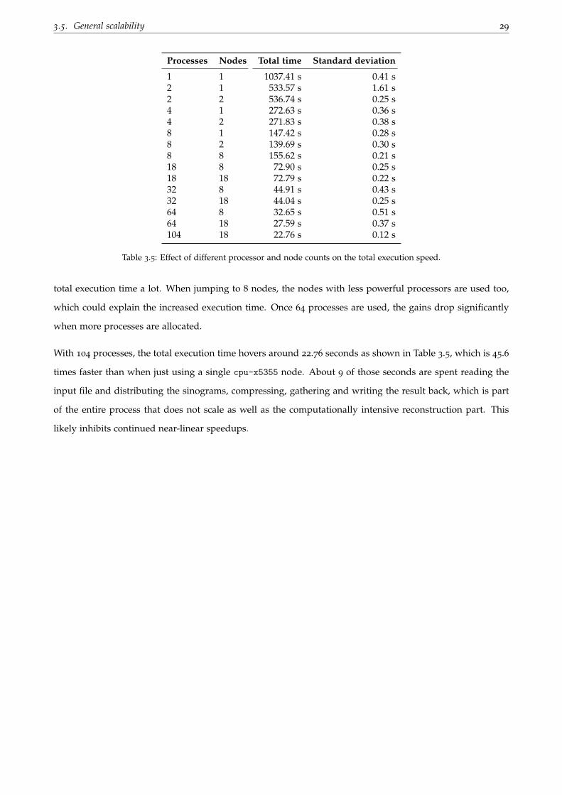
Figure 3.3 shows a plot of these results. Table 3.5 shows the data in tabular form with the standard deviation.

It is clear that, while the implementation does not scale perfectly, it arguably scales fairly well with an

increased number of nodes and processes. An interesting observation is that there is barely any difference

between one and two nodes. Thus, having to transmit data between different nodes did not influence the

3.5. General scalability 29

Processes Nodes Total time Standard deviation

1 1 1037.41 s 0.41 s2 1 533.57 s 1.61 s2 2 536.74 s 0.25 s4 1 272.63 s 0.36 s4 2 271.83 s 0.38 s8 1 147.42 s 0.28 s8 2 139.69 s 0.30 s8 8 155.62 s 0.21 s18 8 72.90 s 0.25 s18 18 72.79 s 0.22 s32 8 44.91 s 0.43 s32 18 44.04 s 0.25 s64 8 32.65 s 0.51 s64 18 27.59 s 0.37 s104 18 22.76 s 0.12 s

Table 3.5: Effect of different processor and node counts on the total execution speed.

total execution time a lot. When jumping to 8 nodes, the nodes with less powerful processors are used too,

which could explain the increased execution time. Once 64 processes are used, the gains drop significantly

when more processes are allocated.

With 104 processes, the total execution time hovers around 22.76 seconds as shown in Table 3.5, which is 45.6

times faster than when just using a single cpu-x5355 node. About 9 of those seconds are spent reading the

input file and distributing the sinograms, compressing, gathering and writing the result back, which is part

of the entire process that does not scale as well as the computationally intensive reconstruction part. This

likely inhibits continued near-linear speedups.

Chapter 4

Application

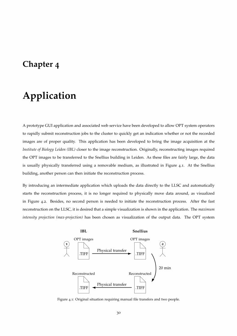
A prototype GUI application and associated web service have been developed to allow OPT system operators

to rapidly submit reconstruction jobs to the cluster to quickly get an indication whether or not the recorded

images are of proper quality. This application has been developed to bring the image acquisition at the

Institute of Biology Leiden (IBL) closer to the image reconstruction. Originally, reconstructing images required

the OPT images to be transferred to the Snellius building in Leiden. As these files are fairly large, the data

is usually physically transferred using a removable medium, as illustrated in Figure 4.1. At the Snellius

building, another person can then initiate the reconstruction process.

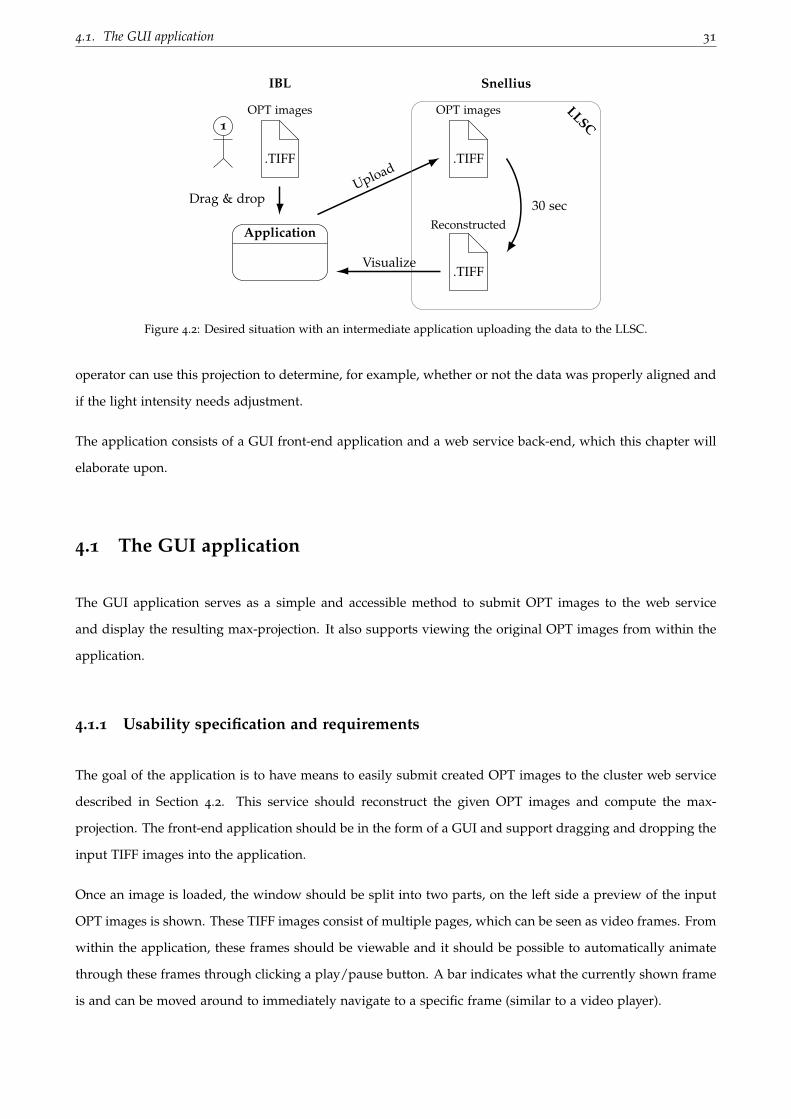
By introducing an intermediate application which uploads the data directly to the LLSC and automatically

starts the reconstruction process, it is no longer required to physically move data around, as visualized

in Figure 4.2. Besides, no second person is needed to initiate the reconstruction process. After the fast

reconstruction on the LLSC, it is desired that a simple visualization is shown in the application. The maximum

intensity projection (max-projection) has been chosen as visualization of the output data. The OPT system

IBL Snellius

.TIFF

OPT images

.TIFF

OPT images

Physical transfer

.TIFF

Reconstructed

20 min

.TIFF

Reconstructed

Physical transfer

1 2

Figure 4.1: Original situation requiring manual file transfers and two people.

30

4.1. The GUI application 31

IBL Snellius

.TIFF

OPT images

.TIFF

OPT images

Upload

.TIFF

Reconstructed

30 secDrag & drop

1

Application

LLSC

Visualize

Figure 4.2: Desired situation with an intermediate application uploading the data to the LLSC.

operator can use this projection to determine, for example, whether or not the data was properly aligned and

if the light intensity needs adjustment.

The application consists of a GUI front-end application and a web service back-end, which this chapter will

elaborate upon.

4.1 The GUI application

The GUI application serves as a simple and accessible method to submit OPT images to the web service

and display the resulting max-projection. It also supports viewing the original OPT images from within the

application.

4.1.1 Usability specification and requirements

The goal of the application is to have means to easily submit created OPT images to the cluster web service

described in Section 4.2. This service should reconstruct the given OPT images and compute the max-

projection. The front-end application should be in the form of a GUI and support dragging and dropping the

input TIFF images into the application.

Once an image is loaded, the window should be split into two parts, on the left side a preview of the input

OPT images is shown. These TIFF images consist of multiple pages, which can be seen as video frames. From

within the application, these frames should be viewable and it should be possible to automatically animate

through these frames through clicking a play/pause button. A bar indicates what the currently shown frame

is and can be moved around to immediately navigate to a specific frame (similar to a video player).

32 Chapter 4. Application

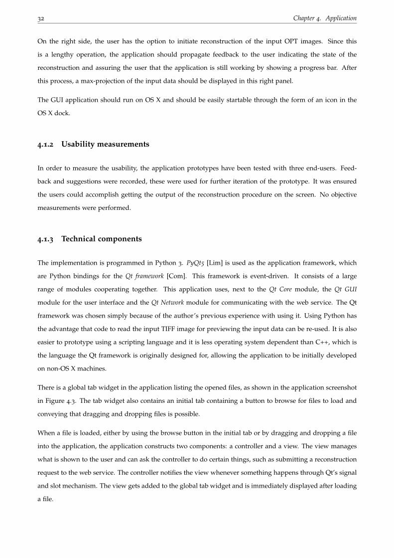
On the right side, the user has the option to initiate reconstruction of the input OPT images. Since this

is a lengthy operation, the application should propagate feedback to the user indicating the state of the

reconstruction and assuring the user that the application is still working by showing a progress bar. After

this process, a max-projection of the input data should be displayed in this right panel.

The GUI application should run on OS X and should be easily startable through the form of an icon in the

OS X dock.

4.1.2 Usability measurements

In order to measure the usability, the application prototypes have been tested with three end-users. Feed-

back and suggestions were recorded, these were used for further iteration of the prototype. It was ensured

the users could accomplish getting the output of the reconstruction procedure on the screen. No objective

measurements were performed.

4.1.3 Technical components

The implementation is programmed in Python 3. PyQt5 [Lim] is used as the application framework, which

are Python bindings for the Qt framework [Com]. This framework is event-driven. It consists of a large

range of modules cooperating together. This application uses, next to the Qt Core module, the Qt GUI

module for the user interface and the Qt Network module for communicating with the web service. The Qt

framework was chosen simply because of the author’s previous experience with using it. Using Python has

the advantage that code to read the input TIFF image for previewing the input data can be re-used. It is also

easier to prototype using a scripting language and it is less operating system dependent than C++, which is

the language the Qt framework is originally designed for, allowing the application to be initially developed

on non-OS X machines.

There is a global tab widget in the application listing the opened files, as shown in the application screenshot

in Figure 4.3. The tab widget also contains an initial tab containing a button to browse for files to load and

conveying that dragging and dropping files is possible.

When a file is loaded, either by using the browse button in the initial tab or by dragging and dropping a file

into the application, the application constructs two components: a controller and a view. The view manages

what is shown to the user and can ask the controller to do certain things, such as submitting a reconstruction

request to the web service. The controller notifies the view whenever something happens through Qt’s signal

and slot mechanism. The view gets added to the global tab widget and is immediately displayed after loading

a file.

4.1. The GUI application 33

Figure 4.3: Screenshot of the prototype GUI application once reconstruction has finished.

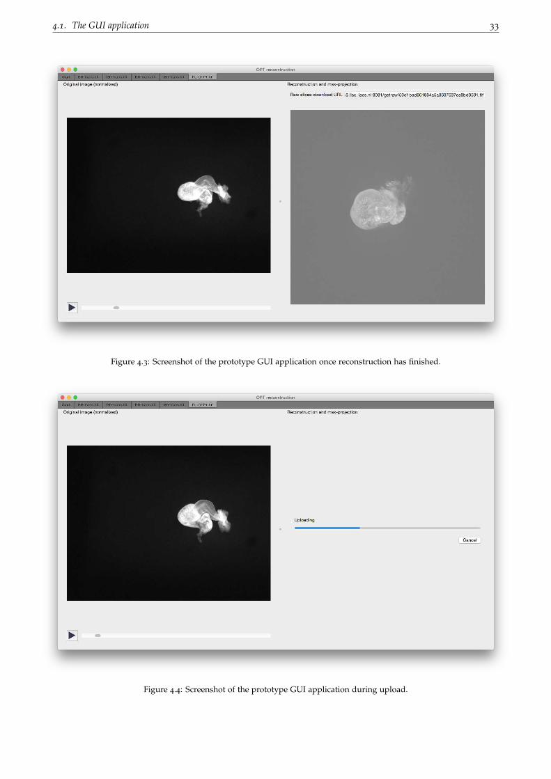
Figure 4.4: Screenshot of the prototype GUI application during upload.


The controller

The controller manages data and loading it from both the web server or the local file system. It thus also

has an internal model to store some data in, although mostly for caching purposes. The controller has the

capability to do the actions listed below.

• Loading a multipage TIFF file representing OPT images from the local file system.

• Requesting to load a specific page from the loaded OPT images asynchronously. The controller uses a

separate worker thread for this, since seeking and loading OPT images takes a significant amount of

time and locking up the UI thread is obviously not desired. The controller notifies the view once an

image has been loaded using a signal. This uses a queue mechanism where the queue has a length of

one. When the queue overflows, older requests are dropped. The read data from the file is cached in

the process’s memory.

• Starting the reconstruction by uploading the entire OPT image file to the web service. The controller

emits signals to the view once a status update is available, like when another chunk of the file has been

uploaded, the reconstruction started or when the entire process finishes. The controller also stores an

internal state of the reconstruction (not started, uploading, reconstructing, succeeded, failed).

• Canceling an earlier started reconstruction.

• Fetching the max-projection from the web service. The controller notifies the view with the image using

a signal once the data arrived.

QNetworkAccessManager is used to communicate with the web service. By hooking to the readyRead signal

of a QNetworkReply, partial responses can be read from the HTTP data stream. By reading and parsing lines

of data from the network buffer as they arrive in the response of a reconstruction request, the application can

read status updates as the web server pushes them (see also Section 4.2.1).

The view

The view consists of two sides with a draggable splitter in-between allowing both sides to be resized. The left

side contains a view of the input OPT image, displaying one page at a time. A scrollbar below the image can

be used to view another image, which signals the controller to load another index. The view connects to a

slot of the controller indicating that an image has loaded. When this happens, the view actually updates the

displayed image. Left to the scrollbar, a play/pause button is located. By pressing the button, the application

will automatically start (or stop) advancing to the next page in the input data every 1/30th of a second. This

button uses icons so that the behavior of this button is quickly recognized. These icons were designed by

4.2. The web service 35

Font Awesome [Gan]. If the system has an icon set built-in, it will try to load these to appear more consistent

with other applications. OS X, however, does not support this by default.

The right side can show different things and is determined by the state of reconstruction. If the reconstruction

has not been started yet, a button is shown to start reconstruction. If it is ongoing, a progress bar and label

indicating the status is shown (Figure 4.4). A cancel button is shown too. When the reconstruction finishes,

the max-projection will be shown in this panel (Figure 4.3).

4.2 The web service

The web service is programmed in Python and utilizes the Tornado Web Framework [Aut]. The module comes

with a built-in web service, making it easy to get it up and running. It runs on a user node on the LLSC.

There are multiple routes defined which the GUI application calls, described in the next sections. The most

fundamental one is the one through which a file can be uploaded to the web service and running the re-

construction request. Whenever this finishes, the max-projection can be requested as a PNG image through

another route. There are a few auxiliary routes defined too for downloading the raw reconstruction result,

downloading a single slice from the reconstruction result and requesting the cluster its job queue. Within this

section, the functionality of the web service will be described.

4.2.1 Submitting a reconstruction request

The route /submitjob can be used to submit reconstruction requests to the web service. It accepts POST

requests whose body is a multipart form data (multipart/form-data) request. This body contains a TIFF

file, used as input for the reconstruction. Once all data is uploaded, the web service computes the MD5 hash

of the entire file. This hash is used to identify the file. The file is saved on the scratch partition on the file

server on the LLSC. Once saved, the actual reconstruction process starts.

Reconstruction

From the web service, qsub is called to schedule a reconstruction job for the saved file. qsub prints the job

id to the standard output stream, which the web service captures. Using this job id, the status of the job can

be polled for completion. Using checkjob the status of a given job can be polled. With the -A parameter,

the output of checkjob is easier to automatically parse. The State attribute from the output of checkjob

is extracted, which indicate that the job may be deferred due to other workload on the cluster, or that it is

currently running. Once the job finishes, checkjob will fail to run. Once the web server notices that checkjob


Reconstructed slices Max-projection

transformedinto

Figure 4.5: Max-projection from a stack of reconstructed slices.

fails, it will verify that the output file exists. If so, the reconstruction is deemed successful, the identifying

MD5 hash it written to the output stream too and the request terminates.

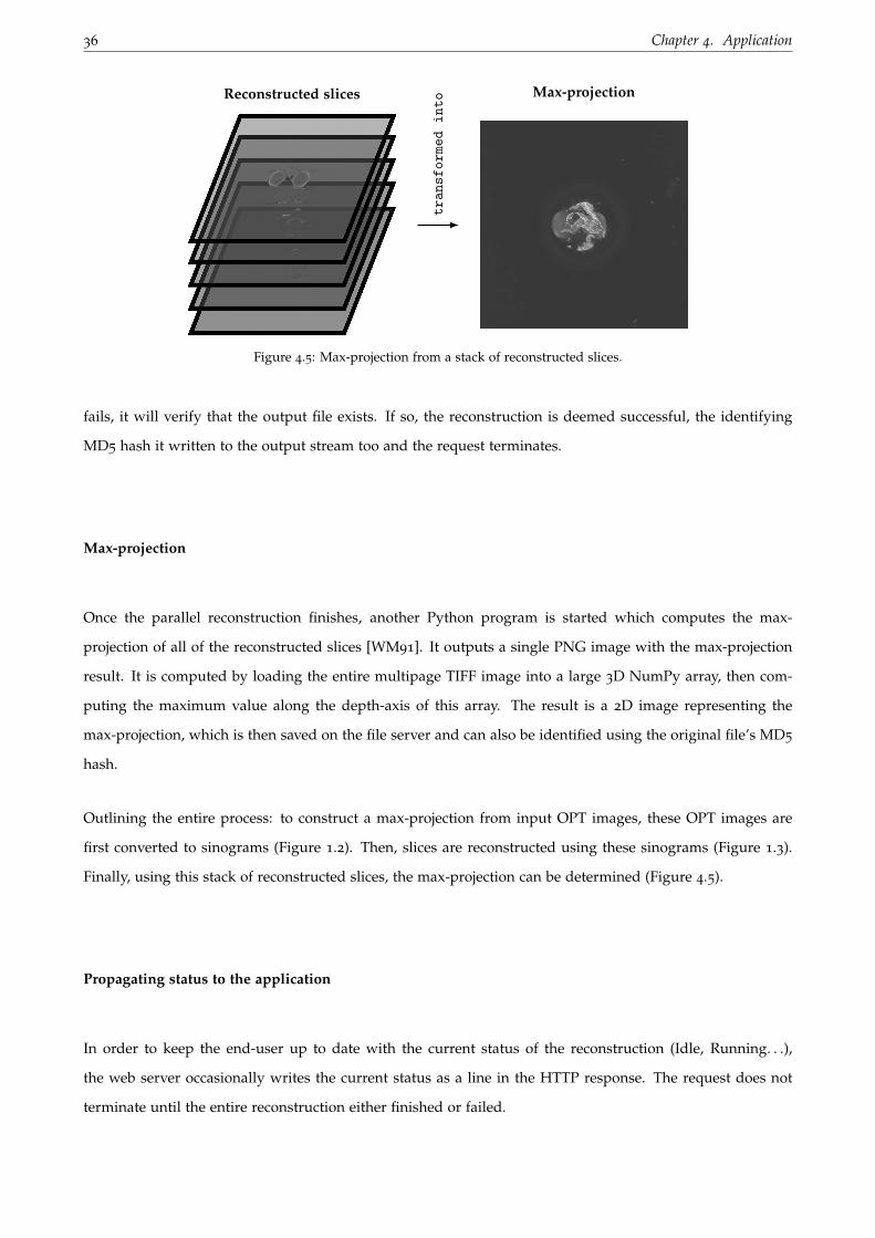
Max-projection

Once the parallel reconstruction finishes, another Python program is started which computes the max-

projection of all of the reconstructed slices [WM91]. It outputs a single PNG image with the max-projection

result. It is computed by loading the entire multipage TIFF image into a large 3D NumPy array, then com-

puting the maximum value along the depth-axis of this array. The result is a 2D image representing the

max-projection, which is then saved on the file server and can also be identified using the original file’s MD5

hash.

Outlining the entire process: to construct a max-projection from input OPT images, these OPT images are

first converted to sinograms (Figure 1.2). Then, slices are reconstructed using these sinograms (Figure 1.3).

Finally, using this stack of reconstructed slices, the max-projection can be determined (Figure 4.5).

Propagating status to the application

In order to keep the end-user up to date with the current status of the reconstruction (Idle, Running. . .),

the web server occasionally writes the current status as a line in the HTTP response. The request does not

terminate until the entire reconstruction either finished or failed.

4.2. The web service 37

4.2.2 Fetching the max-projection

If the reconstruction finishes successfully, the web service has written the identifying MD5 hash of the input

file to the HTTP response body. This MD5 hash can be used with the route /getmproj/([0-9a-f]{32}).png

to get the max projection as a PNG image from the web service. This has already been constructed in the

previous step, so this route serves a static file.

Chapter 5

Conclusions and discussion

5.1 Conclusions

In this thesis it has been researched how well the reconstruction of a sizable set of large OPT images can be

distributed on the LLSC. Experiments have shown that distribution definitely yields significant and scalable

speedups. The gains of distributing the reconstruction in general do reduce when a lot of processes are

allocated, though, as then relatively a lot of time is spent doing I/O-related tasks rather than performing the

computationally expensive inverse radon transform.

Some optimizations to the implementation were developed, ranging from improving the execution speed

of the computationally intensive inverse radon transform, which has a lot positive effect, to optimizations

attempting to improve I/O and IPC times. These optimizations typically have less effect in general, but

mostly compression and streamed TIFF write-back reduce the total execution time significantly.

A usable prototype GUI application has been developed to interface with a developed web service for sub-

mitting reconstruction jobs to the cluster and viewing max-projections of the input OPT images. It allows

OPT system operators to, for example, quickly get an indication whether or not the input OPT images are of

acceptable quality.

5.2 Future work

From this research, several suggestions for future research can be derived. The execution speed and paral-

lelization of the slice reconstruction potentially still has a lot of room for improvement and further research.

On the other hand, the prototype web service and corresponding GUI application also have some ways to go.

38

5.2. Future work 39

5.2.1 Slice reconstruction

To improve the reconstruction speed of the slices, another range of different optimizations can be experi-

mented with. Solutions for parallel reconstruction of a single slice exist, for example. Utilizing this technique

to reconstruct a single slice on an entire node very fast can be compared with the performance of the al-

gorithm in this thesis, where a single process uses one thread to reconstruct a smaller amount of slices.

Different implementations of the inverse radon transform exist in general too, such as a reconstruction based

on the Fourier Slice Theorem instead of a reconstruction based on filtered backprojection as used in this

thesis [Tof96]. These implementations may improve sequential execution speed too.

An entirely different approach can be attempted too, such as using one or multiple GPUs to reconstruct slices

in parallel. Many implementations for filtered backprojections have already been developed and compared

for CUDA [SKKH07, PZM11]. These implementations significantly differ from a implementation for CPUs,

as used in this project. These GPU implementations can potentially be adapted to perform better with a large

amount of sinograms that have to be reconstructed. It could be interesting to research whether or not using

GPUs for slice reconstruction reduces the total execution time and if so, by which factor. I/O times could

minimize potential gains significantly, as observed in the experiment in Section 3.5.

As shown in Section 3.4, parallel compression and streamed TIFF write-back was an optimization that had

most positive influence on the total execution speed of the reconstruction. The performance gains can likely

be improved even more. Currently, the compressed data is first sent to a specific master node that also has to

compress its own data itself. An extra worker process could be introduced living at the file server, to which

the compressed data is immediately sent. This will eliminate the extra data transfer from all worker nodes to

the master node and likely improves performance in general as this process does not have to compress data

itself like other processes living on compute nodes.

Instead of handling the streamed write-back of the TIFF file manually though Irecv and Rsend calls, direct

parallel file writes to the file server can be used too. Instead of allocating large buffers for the output data

in the master process’s memory, a large file can be allocated in which enough space is available for each

process to write their compressed data to, at a pre-determined offset in this file. This obviously results in a

very large file with large parts of the file being unused. Assuming either a Ext4 or a XFS filesystem is used

and that the file server runs Linux kernel 3.15 or newer, the fallocate Linux-function can be used with the

FALLOC FL COLLAPSE RANGE flag to deallocate these unused preallocated file blocks, which then reduces the

file size.

The compression level is also something to consider. Increasing the compression level will reduce the data

size and thus reduce the amount of I/O time, but increases the amount of processing power needed to

actually perform the compression. The experiment in Section 3.4 has shown that with only a few processes,

40 Chapter 5. Conclusions and discussion

the used compression level increases the total execution time. This balance is something that has yet to be

researched and tuned if execution speed is to be maximized.

Finally, because the cluster is not homogeneous, splitting the workload such that each node receives about

an equal amount of slices to reconstruct may not be optimal for the total execution time. Some processors

are significantly faster than others in the cluster. Allocating slices to processes while taking core speed into

account can improve performance even more, especially when many slices are to be reconstructed.

In Section 2.3.1 three alternatives are discussed for constructing a range of sinograms in each of the processes

memory. A limitation of Python modules that read the TIFF files is that they try to serve a general purpose

and full pages at a time, not a select range of scanlines, for performance purposes. A Python-module written

in C can be developed that does something similarly to the first considered variant, in which each process

reads the entire input file and only extracts the rows of pixels it needs. Instead of reading all rows of pixels,

it can skip past scanlines in the input data that worker process does not need at all. This way, less time is

spent reading the file, which may result in less total execution time required for constructing the sinograms.

Each process still seeks through the entire file, but less file reads are issued in total compared to the tested

variant, which could make this optimization effective.

5.2.2 Application

Further work on the GUI application and web service can be done too. Uploading data from the application

to the cluster is fairly slow as it needs to be sent over the internet. Compression on the data stream can

improve the uploading times significantly.

The max-projection is currently computed after the entire reconstruction is written back to an output file on

the file server. It first needs to read this entire file, then compute the max-projection sequentially and then

write back the output max-projection. The distributed slice reconstruction can be extended to also compute

the max-projection in parallel. A local max-projection of the locally reconstructed slices can be computed at

each worker node instead of collecting the reconstructed slices into a TIFF file. These locally reconstructed

slices can then rapidly be reduced to a single global max-projection, which can be saved and sent to the GUI

application. This modification can improve construction of the max-projection significantly.

Currently, the application only shows the max-projection. Alternative views such as the min-projection can

be introduced as well.

The web framework used heavily utilizes coroutines to serve multiple requests at the same time. The con-

trollers written for the web service do not properly yield during long operations, such as computing the

MD5 hash or writing back the input file to the file system and thus lock the entire web server up during these

5.2. Future work 41

operations. Converting these procedures to proper asynchronous operations will enable the server to sustain

multiple requests at once better.

The web service currently uses an in-memory buffer to store partial uploads in. When the upload finishes,

it is all written back at once to the file server which can take about 10 seconds. Writing partially uploaded

data back to a file on the file server as it arrives can improve total execution time of such a reconstruction

request. Besides, with many ongoing uploads, the web server can run out of memory using the current

implementation.

Reconstruction jobs are currently scheduled by the web server in a very crude way. It tries to schedule the

reconstruction job on a fixed amount of nodes. Under load or with few active nodes, this may result in the job

not scheduling in a timely manner. Some metrics can be used to schedule these jobs more cleverly, such as

the amount of nodes currently available. Prioritizing these kind of reconstructions over other batch jobs can

be implemented too. Allocating too few nodes to these reconstruction jobs when more nodes may become

available in the near future may result in the reconstruction finishing significantly later than it could finish.

Research can be performed to schedule these jobs more efficiently.

Currently, the application processes a single scan (one TIFF file with all angles) at a time. Multiple kinds of

scans can be made of the same specimen. These scans belong together and can be visualized as such too,

which a future iteration of the application could integrate. Background masks are often generated too. An

additional preprocessing step could be applied to subtract the background to reduce noise in the output.

Bibliography

[Aut] The Tornado Authors. Tornado web server. http://www.tornadoweb.org/en/stable/.

[Com] The Qt Company. Qt. https://www.qt.io/.

[Dal] Lisandro Dalcin. MPI for Python. https://pythonhosted.org/mpi4py/.

[FEI] FEI. Amira 3d software for life sciences. https://www.fei.com/software/

amira-3d-for-life-sciences/.

[Gan] Dave Gandy. Font awesome. http://fontawesome.io/.

[Inc92] Adobe Systems Incorporated. TIFF. https://partners.adobe.com/public/developer/en/tiff/

TIFF6.pdf, 1992.

[KBK+09] A Kallergi, Y Bei, P Kok, J Dijkstra, J Abrahams, and F Verbeek. Cyttron: A virtualized microscope

supporting image integration and knowledge discovery. Cell Death and Disease Series: Proteins

Killing Tumour Cells, pages 291–315, 2009.

[Lim] Riverbank Computing Limited. What is PyQt? https://www.riverbankcomputing.com/

software/pyqt/intro.

[Orc06] Jeff Orchard. iradon speedy. https://www.mathworks.com/matlabcentral/fileexchange/

12852-iradon-speedy, 2006.

[Pro] The Open MPI Project. Open MPI: Open source high performance computing. https://www.

open-mpi.org/.

[PZM11] Eric Papenhausen, Ziyi Zheng, and Klaus Mueller. GPU-accelerated back-projection revisited:

squeezing performance by careful tuning. In Workshop on High Performance Image Reconstruction

(HPIR), pages 19–22, 2011.

[Sha04] James Sharpe. Optical projection tomography. Annual Review of Biomedical Engineering, 6:209–228,

2004.

42

http://www.tornadoweb.org/en/stable/

https://www.qt.io/

https://pythonhosted.org/mpi4py/

https://www.fei.com/software/amira-3d-for-life-sciences/

https://www.fei.com/software/amira-3d-for-life-sciences/

http://fontawesome.io/

https://partners.adobe.com/public/developer/en/tiff/TIFF6.pdf

https://partners.adobe.com/public/developer/en/tiff/TIFF6.pdf

https://www.riverbankcomputing.com/software/pyqt/intro

https://www.riverbankcomputing.com/software/pyqt/intro

https://www.mathworks.com/matlabcentral/fileexchange/12852-iradon-speedy

https://www.mathworks.com/matlabcentral/fileexchange/12852-iradon-speedy

https://www.open-mpi.org/

https://www.open-mpi.org/

BIBLIOGRAPHY 43

[sidt] The scikit-image development team. scikit-image — module: transform. http://scikit-image.

org/docs/dev/api/skimage.transform.html.

[SKKH07] Holger Scherl, Benjamin Keck, Markus Kowarschik, and Joachim Hornegger. Fast GPU-based CT

reconstruction using the common unified device architecture (CUDA). In Nuclear Science Sympo-

sium Conference Record, 2007. NSS’07. IEEE, volume 6, pages 4464–4466. IEEE, 2007.

[Tan16] Xiaoqin Tang. Fluorescence and bright-field 3d image fusion based on sinogram unification for

optical projection tomography. Unpublished work, 2016.

[Tof96] Peter Toft. The Radon Transform: Theory and Implementation : Ph.d. Thesis. Department of Mathemat-

ical Modelling, Section for Digital Signal Processing, Technical University of Denmark, 1996.

[WM91] Jerold W Wallis and Tom R Miller. Three-dimensional display in nuclear medicine and radiology.

Journal of nuclear medicine: official publication, Society of Nuclear Medicine, 32(3):534–546, 1991.

http://scikit-image.org/docs/dev/api/skimage.transform.html

http://scikit-image.org/docs/dev/api/skimage.transform.html

Documents

UniversiteitLeiden OpleidingInformaticaliacs.leidenuniv.nl/assets/Bachelorscripties/Inf-studiejaar-2015... · UniversiteitLeiden OpleidingInformatica ... input images and view a