Embed Size (px)
Citation preview
UNIVERSITY OF CALGARY
Kinetics of Asphaltene Precipitation and Flocculation from Diluted Bitumen
by
Mahdieh Shafiee Neistanak
A THESIS
SUBMITTED TO THE FACULTY OF GRADUATE STUDIES
IN PARTIAL FULFILMENT OF THE REQUIREMENTS FOR THE
DEGREE OF MASTER OF SCIENCE
GRADUATE PROGRAM IN CHEMICAL AND PETROLEUM ENGINEERING
DEPARTMENT
CALGARY, ALBERTA
July, 2014
© Mahdieh Shafiee Neistanak 2014
ii
Abstract
The kinetics of the precipitation and flocculation of asphaltenes can impact the operation of solvent
deasphalting processes such as paraffinic froth treatment as well as the potential for deposition from
destabilized crude oil. It has also been reported that the solvent content at which asphaltenes
precipitate (the onset condition) is a time dependent property and may be far lower than reported
because the precipitation kinetics are slow. However, it is possible that the slow kinetics are caused
by oxidation or oxygen catalyzed polymerization.
The objectives of this thesis are to: 1) assess the role of oxygen in asphaltene precipitation kinetics;
2) determine the kinetics of asphaltene precipitation from diluted bitumen near the onset of
precipitation, and; 3) investigate the kinetics of asphaltene flocculation near the onset of
precipitation. The data were collected from a Western Canadian bitumen diluted with n-heptane at
23oC. The n-heptane content at the onset of precipitation was determined using a combination of
optical microscopy and gravimetric analysis. Asphaltene precipitate yields were measured over
time gravimetrically, and asphaltene flocculation was investigated using a Lasentec particle size
analyzer.
The onset of asphaltene precipitation (defined as the first appearance of 0.5 µm asphaltene
particles) in n-heptane diluted bitumen occurred at 57.5 wt% heptane. When heptane was added
above the onset amount, precipitation yields increased at an exponentially decaying rate over 48
hours. In air, the yields increased and the onset n-heptane content decreased at a slow rate for at
least a month. In nitrogen, the yields reached a plateau and there was no change in the onset
iii
condition after 48 hours. Once oxygen related artifacts were eliminated, the precipitation kinetics
could be described with first order kinetics requiring an ultimate yield and a rate constant. The
steady state yield is a function of the solvent content and has been modeled with regular solution
theory. A single rate constant was found to apply to all of the data.
The effects of heptane content and shear rate on the kinetics of asphaltene flocculation were
investigated and modeled using a population balance based model adopted from Rastegari et al.
(2004) and Daneshvar (2005). Unfortunately, the particle size analyzer could not detect the particle
size distribution in unadulterated bitumen near the onset. Therefore, data was collected at dilutions
well above the onset and the possibility of extrapolating the model to near onset conditions
investigated.
The main parameters governing flocculation are the particle concentration, the fractal dimension,
and the magnitude and ratio of the flocculation and shattering rates, kf/ks. The fractal dimension of
settled flocs was found to be 2.3 ±0.1 (with a slight dependence on the n-heptane content) and this
value was assumed to apply for suspended flocs. At the dilutions considered in this thesis, adding n-
heptane decreased the individual particle concentration and therefore decreased flocculation. An
increase in the shear rate resulted in a decrease in the asphaltene volume mean diameter, while the
total number of asphaltene flocs in the mixture remained relatively constant. This observation
indicates that asphaltene flocs likely become more compact at higher shear rates.
The flocculation model was fitted the data at different dilutions. A constant value of the shattering
rate was sufficient to fit the data. Both the fractal dimension and the reaction rate ratio could be
iv
correlated to the mass fraction of n-heptane. The effect of shear rate on the kf/ks ratio at various
heptane contents was investigated for two different bitumen samples. The kf/ks ratio appears to
decrease with increasing Reynolds number up to 12000, above which the ratio becomes constant.
The decrease in the ratio corresponds to the transition zone, while the plateau corresponds to the
establishment of a turbulent zone.
While the model parameters could be correlated to n-heptane content, a long extrapolation with a
significant a change in parameter values is required to estimate the behavior near the onset
condition. Hence, the flocculation rates near the onset conditions cannot be determined from the
available data with any confidence. It is recommended that data be collected for toluene-bitumen
feedstocks where the onset occurs at higher n-heptane contents so that a more reliable extrapolation
can be performed. If successful, both precipitation and flocculation rates can be predicted and used
to guide process design and operation.

v
Acknowledgements
I would like to express my deepest and profound gratitude to my supervisor, Dr. Harvey Yarranton
for his constant support and encouragement throughout the course of this study. This work would
not have been possible without his guidance and support. It was an honour and a privilege to be part
of his research group and work under his supervision toward my master degree.
I am particularly grateful to Florian Schoeggl, our PVT lab manager, for his constant support and
assistance throughout the experimental work of my study. I would like to acknowledge his
contribution in teaching me the experimental work of my study. He was very patient with me in the
lab.
I am thankful to the Department of Chemical and Petroleum Engineering, Faculty of Graduate
Studies at the University of Calgary, for providing wonderful facilities and a great educational
ambience. I am also grateful to NSERC for their financial support throughout my Master program.
I am also thankful to Elaine Baydak and Hamed Reza Motahhari for their assistance and great help
during my master’s thesis. I am grateful to have worked with the members of the Asphaltene and
Emulsion Research Group and fellow graduate students.
Finally I am profoundly indebted to my parents, for their constant support, dedications and
continuous inspiration throughout all stages of my life. I express my gratitude to my dear brothers
and caring sister and my lovely friend, Niloufar Hojati, for their continues support and
encouragements during the course of my Master study.

vi
Dedication
To my parents, Mohammad Ebrahim and Soraya
To my brothers, Mojtaba and Mohammad
To my sister, Maryam
vii
Table of Contents
Chapter One:INTRODUCTION ..................................................................................................... 1
1.1 Background ........................................................................................................................... 1
1.2 Research Objectives .............................................................................................................. 6
1.3 Brief Overview of Chapters .................................................................................................. 7
Chapter Two: LITERATURE REVIEW ........................................................................................ 9
2.1 Asphaltene Chemistry ........................................................................................................... 9
2.1.1 Asphaltene Molecular Structure .................................................................................. 10
2.1.2 Asphaltene Self-Association ........................................................................................ 11
2.2 Asphaltene Precipitation ..................................................................................................... 13
2.2.1 Asphaltene Precipitation Kinetics ................................................................................ 17
2.3 Asphaltene Flocculation...................................................................................................... 20
2.3.1 Floc Structure and Fractal Dimension ......................................................................... 21
2.3.2 Factors Affecting Asphaltene Flocculation ................................................................. 23
2.4 Asphaltene Flocculation Modeling ..................................................................................... 27
2.4.1 Flocculation Models in General ................................................................................... 27
2.4.2 Irreversible Flocculation .............................................................................................. 28
2.4.3 Reversible Flocculation ............................................................................................... 31
2.4.4 Asphaltene Flocculation Models.................................................................................. 33
Chapter Three: EXPERIMENTAL METHODS .......................................................................... 36
3.1 Materials ............................................................................................................................. 36
3.2 Precipitation Measurements ............................................................................................... 37
3.2.1 Asphaltene Yield Measurement .................................................................................... 37
3.2.2 Onset of Precipitation – Gravimetric Method............................................................... 40
3.2.3 Onset of Precipitation – Microscopy Method ............................................................... 41
3.3 Flocculation Measurements ............................................................................................... 42
3.3.1 Particle Size Analyzer ................................................................................................... 42
3.3.2 Flocculation Experiments ............................................................................................. 48
Chapter Four: KINETICS OF ASPHALTENE PRECIPITATION ............................................. 52
viii
4.1 Onset of Asphaltene Precipitation in n-Heptane Diluted Bitumen ..................................... 52
4.1.1 Onsets from Microscopic Method ............................................................................... 52
4.1.2 Gravimetric Observations ............................................................................................ 55
4.2 Asphaltene Yields over Time in n-Heptane Diluted Bitumen ............................................ 58
4.3 Asphaltene Onset and Yield in n-Pentane Diluted Bitumen ............................................... 63
Chapter Five: ASPHALTENE FLOCCULATION MODEL ....................................................... 68
5.1 Smoluchowski Population Balance Equation for Asphaltene Flocculation Model ............ 68
5.2 Flocculation and Disintegration Reaction Terms ............................................................... 69
5.2.1 Flocculation Reaction Term ......................................................................................... 70
5.2.2 Disintegration Reaction Term ...................................................................................... 71
5.3 Fractal Dimension ............................................................................................................... 71
5.4 Computer Flow Chart to Solve Population Balance Equation............................................ 75
Chapter Six: ASPHALTENE FLOCCULATION RESULTS ...................................................... 79
6.1 Asphaltene Flocculation Measurements ............................................................................. 79
6.1.1 Processing of Flocculation Data .................................................................................. 79
6.1.2 Flocculation Data near the Onset of Asphaltene Precipitation .................................... 82
6.1.3 Flocculation Data at High Dilution .............................................................................. 91
6.2 Asphaltene Aggregate Fractal Dimension .......................................................................... 99
6.3 Modeling of Asphaltene Flocculation ............................................................................... 103
6.3.1 Model Input ................................................................................................................ 103
6.3.2 Model Fitting – Constant Df ...................................................................................... 105
6.3.3 Correlation of Model Parameters to n-Heptane Content – Constant Df .................... 108
6.3.4 Model Fitting –Df as Function of n-Heptane Content ............................................... 116
6.3.5 Effect of Shear Conditions – Constant Df .................................................................. 118
6.3.6 Sensitivity to Model Parameters – Constant Df ......................................................... 121
6.3.7 Summary .................................................................................................................... 131
Chapter Seven: CONCLUSIONS AND RECOMMENDATIONS ............................................ 132
7.1 Conclusions ....................................................................................................................... 132
7.2 Recommendations For Future Study ................................................................................ 135
References ................................................................................................................................... 137

ix
APPENDIX A: Average Absolute Relative Deviation ............................................................. 143
APPENDIX B: Asphaltene Bins .............................................................................................. 145
x
List of Tables
Table 2.1: The elemental composition of asphaltenes from various Canadian regions, (Speight,
2006). ......................................................................................................................................... 11
Table 3.1: SARA composition of WCB2 bitumen. ........................................................................... 37
Table 3.2: Summary of Reynolds number corresponding to each dilution ratio and mixing speed
at 23oC. ....................................................................................................................................... 50
Table 4.1: Onset of asphaltene precipitation in n-heptane and n-pentane diluted WC_B2
bitumen at 23°C and 1 atm. ........................................................................................................ 53
Table 5.1: Mass fractal dimension of a floc. ...................................................................................... 75
Table 6.1: Parameters employed in each step to match the experimental volume mean diameter. . 105
Table 6.2: Fitted model parameters (Case 1) for n-heptane diluted bitumen with two-stage
mixing method and a mixing speed of 195 rpm at 23°C. ........................................................ 109
xi
List of Figures and Illustrations
Figure 2.1: ASTM D2007 SARA fractionation procedure. ............................................................... 10
Figure 2.2: Micrograph of asphaltenes precipitated from a solution of asphaltenes in toluene and
n-heptane (adapted from Rastegari et al., 2004). ....................................................................... 14
Figure 2.3: The gravimetrically determined onset and yield of asphaltene precipitation from n-
heptane diluted with Athabasca bitumen at 24 hours at 23°C (adapted from Beck et al.,
2005). ......................................................................................................................................... 15
Figure 3.1:Photograph of the nitrogen atmosphere inflatable glove box. .......................................... 40
Figure 3.2: Gravimetric determination of the onset of asphaltene precipitation from n-heptane
diluted bitumen at 2 hours by extrapolation of asphaltene yield data to zero yield. .................. 41
Figure 3.3: Comparison between measured and given volume frequency distribution of a
standard sample of 8.33 wt/wt% PVC particles suspended in water at 400 rpm and 23oC. ...... 46
Figure 3.4: Measured volume mean diameter and particle count distribution for a) low dilution
of 62 wt%, and b) high dilution of 87.5 wt% n-heptane, at 195 rpm and 23oC. ........................ 47
Figure 3.5: Diagram of the beaker with mixer and the probe. ........................................................... 48
Figure 3.6: a) Number frequency distribution, and b) volume frequency distribution of
asphaltene flocs for three different runs after 10 minutes for 87.5 wt% n-heptane, at 195
rpm, and 23oC. ........................................................................................................................... 51
Figure 4.1: Micrographs showing the onset of asphaltene precipitation from n-heptane diluted
WC_B2 bitumen at a) 56.5 wt%, b) 57.0 wt%, and c) 57.5 wt% n-heptane in air at 23°C. ..... 54
Figure 4.2: Gravimetric determination of the onset of asphaltene precipitation from n-heptane
diluted WC_B2 bitumen at 2 hours by extrapolation of asphaltene yield data to zero yield
at 23°C. ...................................................................................................................................... 55
Figure 4.3: Comparison of gravimetric and microscopic precipitation onsets up to 48 hours in n-
heptane diluted a) WC_B2 (Shafiee, 2014) and b) WC_B3 (Motahhari, 2013) bitumen in
air at 23°C and 1 atm. Error bars in yield of ±0.61 wt% are not shown to avoid clutter. .......... 56
Figure 4.4: Gravimetric precipitation onsets in n-heptane diluted WC_B2 bitumen in air and
nitrogen (Shafiee, 2014), and n-heptane diluted k-1 crude oil (Maqbool et al. 2009) at 23°C
and 1 atm. ................................................................................................................................... 58
Figure 4.5: Comparison of asphaltene kinetics from WC_B2 bitumen (Shafiee, 2014) and k-1
crude oil (Maqbool et al., 2009), both diluted with n-heptane in air at 23°C and 1 atm.
Error bars in yield of ±0.61 wt% (Shafiee, 2014), and ±0.41 wt% (Maqbool et al., 2009)
are not shown to avoid clutter. ................................................................................................... 59
xii
Figure 4.6: Comparison of asphaltene kinetics from WC_B2 bitumen (Shafiee, 2014) and
Athabasca bitumen (Beck et al., 2005) both diluted with n-heptane in air at 23°C and 1
atm. Error bars in yield of ±0.61 wt% (Shafiee, 2014), and ±0.75 wt% (Beck et al., 2005)
are not shown to avoid clutter. ................................................................................................... 59
Figure 4.7: Comparison of asphaltene kinetics from WC_B2 bitumen (Shafiee, 2014) and
Athabasca bitumen (Beck et al., 2005) both diluted with n-heptane in Nitrogen at 23°C and
1 atm. Error bars in yield of ±0.61 wt% (Shafiee, 2014), and ±0.75 wt% (Beck et al., 2005)
are not shown to avoid clutter. ................................................................................................... 60
Figure 4.8: Comparison of asphaltene yields from n-heptane diluted WC_B2 bitumen over time
in air and nitrogen at 23°C and 1 atm. Error bars in yield of ±0.61 wt% are not shown to
avoid clutter. .............................................................................................................................. 61
Figure 4.9: Asphaltene precipitation over longer run from WC_B2 bitumen diluted with n-
heptane in air at 23oC and 1 atm. ............................................................................................... 62
Figure 4.10: Measured and fitted asphaltene yields over time from n-heptane diluted
WC_B_B02 bitumen in a nitrogen atmosphere at 23°C and 1 atm. .......................................... 63
Figure 4.11: Micrographs showing the onset of asphaltene precipitation from n-pentane diluted
WC_B2 bitumen at 49 wt% n-pentane in air at 23°C. ............................................................... 64
Figure 4.12: Comparison of gravimetric and microscopic precipitation onsets up to 48 hours in
n-pentane diluted WC_B_B03 (Motahhari, 2013) bitumen in air at 23°C and 1 atm. .............. 65
Figure 4.13: Asphaltene precipitation from WC_B_B03 bitumen (Motahhari, 2013) diluted with
n-pentane in air at 23oC and 1 atm. ............................................................................................ 66
Figure 5.1: Schematic of a floc with fractal structure. ....................................................................... 73
Figure 6.1: Measured asphaltene floc number (a) and volume frequency (b) distributions after 5
and 30 minutes for 87.5 wt% n-heptane diluted bitumen using two-stage mixing method at
195 rpm and 23°C. ..................................................................................................................... 81
Figure 6.2: Volume mean diameter and number count of asphaltene flocculation over time from
87.5 wt% n-heptane diluted bitumen using the two-stage mixing method at a mixing speed
of 195 rpm, and 23°C. ................................................................................................................ 82
Figure 6.3: Kinetics of asphaltene flocculation at low dilutions of a) 61.5 wt% and b) 65 wt% n-
heptane using two-stage mixing method at 195 rpm, and 23oC................................................. 83
Figure 6.4: Measured volume frequency distribution for low and high n-heptane (C7) diluted
bitumen after 60 minutes using two-stage mixing method at 195 rpm, and 23oC. .................... 84
Figure 6.5: Comparison of measured number count (a) and measured volume mean diameter (b)
with concentration of precipitated asphaltenes based on the yield data for 24 hours
presented in Chapter 4 at 23oC. .................................................................................................. 86
xiii
Figure 6.6: Micrographs showing a high volume of visible particles at both a) 61.5 and b) 87.5
wt% n-heptane at 23oC. .............................................................................................................. 87
Figure 6.7: Volume mean diameter and particle count measurements at longer time for 61.5
wt% n-heptane, using two-stage mixing method at 195 rpm, and 23oC. ................................... 88
Figure 6.8: Volume mean diameter and particle count measurements at longer time for a) 64.5
wt% n-heptane and b) 70 wt% n-heptane in bitumen diluted with toluene at a 1:1 mass
ratio (two-stage mixing method at 195 rpm, and 23oC). Note: the two plots are not on the
same scale. ................................................................................................................................. 90
Figure 6.9: Kinetics of asphaltene flocculation for various n-heptane contents: (a) on the volume
mean diameter and (b) the number count rate for two-stage mixing with a mixing speed of
195 rpm, 23oC. ........................................................................................................................... 92
Figure 6.10: Effect of n-heptane content on the volume mean diameter and the number count
rate after 30 minutes in the two-stage mixing method at 195 rpm, and 23oC. ........................... 94
Figure 6.11: Effect of mixing scheme on the steady state volume mean diameter of asphaltene
flocs after 30 minutes at 195 rpm and 23oC. .............................................................................. 96
Figure 6.12: Effects of mixing scheme on the kinetics of asphaltene flocculation for 90.5 wt%
n-heptane, at 195 rpm and 23oC. ................................................................................................ 97
Figure 6.13: Effect of shear rate (mixing rate) on the steady state volume mean diameter and
number count rate for 87.5 wt% n-heptane using two-stage mixing scheme at 23°C. .............. 98
Figure 6.14: Micrograph of floc showing the area and perimeter used to determine the fractal
dimension in 87.5 wt% n-heptane in bitumen at 23°C ............................................................ 101
Figure 6.15: Determination of perimeter-based asphaltene aggregates fractal dimension from
image analysis of flocs from 87.5 wt% n-heptane in bitumen at 23°C. ................................... 101
Figure 6.16: Fractal dimension determined based on sediment volume of 25% for dilutions of
87.5 to 95.5 wt% diluted in n-heptane. .................................................................................... 103
Figure 6.17: Comparison between measured and the converted initial bin cumulative number
frequency for 87.5 wt% n-heptane using two-stage mixing method at 195 rpm, and 23oC. ... 104
Figure 6.18: The fitted and experimental volume mean diameter for 87.5 wt% n-heptane using
two-stage mixing method at 195 rpm, and 23oC. ..................................................................... 106
Figure 6.19: Predicted and experimental cumulative volume frequencies for the case study after:
a) 10 minutes and b) 30 minutes. ............................................................................................. 107
Figure 6.20: Case 1 model fitted to data for 87.5-95.5 wt% n-heptane diluted bitumen using the
two-stage mixing method and a mixing speed of 195 rpm at 23oC. ........................................ 109

xiv
Figure 6.21: Case 2 (constant ks) model fitted to data for 87.5 to 95.5 wt% n-heptane diluted
bitumen using the two-stage mixing method and a mixing speed of 195 rpm at 23oC. .......... 111
Figure 6.22: The kf/ks ratio for each fitting step for 87.5 to 95.5 wt% n-heptane diluted bitumen
using the two-stage mixing method and a mixing speed of 195 rpm at 23oC.......................... 111
Figure 6.23: Case 3 (constant kf/ks ratio and ks) model results for 87.5 to 95.5 wt% n-heptane
diluted bitumen using the two-stage mixing method and mixing speed of 195 rpm at 23oC. . 112
Figure 6.24: Case 4 (correlated kf/ks ratio and constant ks) model results for 87.5 to 95.5 wt% n-
heptane diluted bitumen using the two-stage mixing method and mixing speed of 195 rpm
at 23oC. ..................................................................................................................................... 112
Figure 6.25: Effect of heptane content on the kf/ks ratio (Case 4) for W_B02 and Athabasca
diluted bitumen using the two-stage mixing method and a mixing speed of 195 rpm at
23oC. ......................................................................................................................................... 114
Figure 6.26: Sensitivity of model predictions to kf/ks ratios extrapolated to 87.5 wt% n-heptane
with different slopes: a) extrapolated kf/ks extrapolation; b) predictions for 87.5 wt% n-
heptane in W_B02 bitumen using the two-stage mixing method and mixing speed of 195
rpm at 23oC. ............................................................................................................................. 115
Figure 6.27: Correlated kf/ks ratio and constant ks model results based on true fractal dimension
for 87.5 to 95.5 wt% n-heptane diluted bitumen using the two-stage mixing method and
mixing speed of 195 rpm at 23oC............................................................................................. 117
Figure 6.28: The kf/ks ratio for the true fractal dimension for 87.5 to 95.5 wt% n-heptane diluted
bitumen using the two-stage mixing method and a mixing speed of 195 rpm at 23oC. .......... 117
Figure 6.29: Effect of adjusting Df on the volume frequency distribution for 87.5 wt% n-
heptane diluted bitumen using the two-stage mixing method and a mixing speed of 195
rpm at 23oC. ............................................................................................................................. 118
Figure 6.30: Summary of kf/ks ratio for a) 87.5-95.5 wt% at 195 rpm and 87.5 wt% at different
shear, b) comparison of two bitumen, WC_B02 and Athabasca. ............................................ 120
Figure 6.31: Effect of ks on the predicted a) volume mean diameter and b) number counts. .......... 122
Figure 6.32: Effect of adjusting a) ks and b) β on the volume frequency distribution. .................... 123
Figure 6.33: Effect of disintegration reaction exponent on the predicted a) volume mean
diameter and b) number counts. ............................................................................................... 124
Figure 6.34: Effect of flocculation reaction exponent on the predicted a) volume mean diameter
and b) number counts. .............................................................................................................. 125
Figure 6.35: Effect of adjusting a) β and b) λ on the volume frequency distribution. .................... 126
xv
Figure 6.36: Effect of fractal dimension on the predicted a) volume mean diameter and b)
number counts. ......................................................................................................................... 128
Figure 6.37: Effect of adjusting Df on the volume frequency distribution. ..................................... 129
Figure 6.38: Effect of lower limit cluster size on a) volume mean diameter, and b) volume mean
diameter distributions. .............................................................................................................. 130
xvi
List of Symbols, Abbreviations and Nomenclature
Symbol Definition
A Area
Ck Mass concentration of particle k
Ci Mass concentration of particle i
Cj Mass concentration of particle j
P Perimeter
Df Fractal Dimension
D(i,j) Disintegration reaction kernel (number of reactions per unit volume
per unit time)
D dimension
di Measured diameter of floc i
dfloc Measured diameter of a floc
dm Spherical mean diameter of a floc
dp Diameter of an individual particle
Df Fractal dimension
Di Disintegration reaction kernel
fi Number frequency of floc i
Fi,j Flocculation reaction constant (number of reactions per unit volume
per unit time)
k Particle k
K Boltzmann Constant
Ks non-dimensional constant
kf Flocculation reaction constant in terms of number of individual
particles in flocs
kf /ks Ratio of flocculation and disintegration reaction constant
kd Disintegration reaction constant in terms of number of individual
particles in flocs
k¢f Flocculation reaction constant in terms of mass of flocs
mA Mass of precipitated asphaltene
m i mass of ith floc
Mk Mass of particle of particle k
Mj Mass of particle of particle j
Mi Mass of particle of particle i
F(i,j) flocculation reaction rate (number of reactions per unit volume per
unit time)
F(i,k) flocculation reaction rate (number of reactions per unit volume per
unit time)
N Number of particles in a cluster
xvii
N Mixing Speed (min-1) used in Equation 3. 1
nbin Number of asphaltene bins with sizes between approximately 18 and
396 microns
nf Number of individual (primary) particles in a floc
ni Number of particles in the floc i
nj Number of particles in the floc j
nmin Number of individual particles in the smallest asphaltene bin
nmax Number of individual particles in the biggest asphaltene bin
n1 Number of individual particles in an asphaltene bin size of 18
microns
dimp impeller diameter (inch
n2 Number of individual particles in an asphaltene bin size of 396
microns
Nf Total number of flocs
Nre Reynolds number
Nt Total number of individual particles in the solution
Rg Radius of gyration
Ri Radius of a floc
Ri+j Radius of floc I an j
s Sample variance
Y yield (w/w)
Yeq equilibrium yield (w/w)
Sf Scaling factor
t Time
T Absolute temperature
vi Volume of particle i
vj Volume of particle j
Vactual Actual volume of a floc
Vapp Apparent volume of a floc
Vtotal The total apparent volume of a distribution of flocs
MBerr material balance error at each time step
Greek Symbol Definition ϒ Shear rate (s-1)
α = 1 – (%conf/100)
β Disintegration exponent
λ Flocculation exponent
ρA Density of pure asphaltene
ρm Mixture density (g/cc)
µ Viscosity of medium (mPa.s)
1
CHAPTER ONE: INTRODUCTION
1.1 Background
Mineable oil sands compose a significant proportion, as much as 30%, of the world’s known oil
reserves (Atkins and MacFadyen, 2008). An average grade oil sand contains approximately 10
wt% bitumen, 1-2 wt% water, and 88 wt% solids of which 3 to 30% are fine solids (Romanova et
al., 2006). Commercial bitumen processes recover this relatively small fraction of bitumen from
the oil sands using two steps: water based extraction and solvent based froth treatment.
Water based extraction was developed by Clark and Pasternack (1932) and involves mixing the
oil sand with hot water and, if necessary, sodium hydroxide to separate bitumen from the sand
matrix (Chalaturnuk and Scott, 2004). The hot water and hydroxide release natural surfactants
from the oil sand which promote detachment of bitumen from the sand and attachment of the
bitumen to air bubbles. The mixture is aerated and tumbled to produce a froth containing
approximately 65 wt% bitumen, 25% water, and 10 wt% sands and clays (Sanford and Seyer,
1979; Kotlyar et al., 1998). The froth must be treated separately to separate the bitumen from the
remaining water and solids.
There are two commercial froth treatment processes, one based on naphtha and one based on a
paraffinic solvent. In the naphtha based process, used by Syncrude and Suncor, the froth is
diluted with naphtha to reduce the density and viscosity of the bitumen and the remaining water
and solids are removed by centrifugation. In the paraffinic process, used by Albian, a paraffinic
2
solvent is added and the water and solids are removed by gravity settling. The paraffinic solvent
not only reduces the density and viscosity of the bitumen but also precipitates some of the
asphaltenes (the heaviest, most aromatic oil constituents) and promotes flocculation of the
emulsified water and suspended solids (Long et al., 2002; Romanova et al., 2006). The paraffinic
process has a lower bitumen recovery than the naphthenic process because the precipitated
asphaltenes are rejected to the tailings stream along with the water and solids. On the other hand,
the naphthenic process produces more coke during upgrading because the asphaltenes remain in
the bitumen.
Some problems associated with water based extractions are their low energy efficiency, high
water usage, and the creation of a tailings stream with poor consolidation properties
(Chalaturnuk and Scott, 2004). An alternative is solvent based oil sands extraction, which
substantially reduces water consumption and eliminates the need for froth treatment and tailings
ponds. However, there are still some unresolved issues in solvent based extraction, such as the
optimization of bitumen recovery for the target upgrading process, the production of a clean
bitumen product, and the removal of solvent from rejected sand and water tailings (Yarranton,
2012). Imperial Oil has recently patented several non-aqueous process options, which address
most of these issues (Adeyinka et al., 2010). The proposed processes involve sequential
separations and fine agglomeration. Reportedly, the processes give high bitumen recovery, a
bitumen product that meets pipeline specifications, and efficient solvent recovery. Nonetheless,
approximately 1 wt% fine solids remain in the bitumen product (Mayer, 2011). There may also
be room to optimize the solvent-to-bitumen (S/B) ratios used in different process variations.
3
One method to remove the fine solids is to use a high dilution of a paraffinic solvent to
precipitate asphaltenes and induce flocculation and settling, as is done in paraffinic froth
treatment. This method would provide a clean bitumen product, much like paraffinic froth
treatment. However, high dilutions are economically disadvantageous. A potential alternative is
to design this stage of the process to operate near the onset of asphaltene precipitation in order to
minimize both solvent requirements and asphaltene rejection. Also, precipitated asphaltenes
contain some solvent, which can be very difficult to recover (George et al., 2009). Hence,
minimizing precipitation may also minimize ultimate solvent losses. For this process to work, the
suspended solids must still be flocculated and settled in a practical time frame.
Two factors make the process conceptually feasible. First, asphaltenes are often adsorbed on the
surface of solids (Yan et al., 2001); and therefore, these particles tend to flocculate in solvents
that are incompatible with asphaltenes (Saadatmand et al., 2009). Second, the kinetics of
asphaltene precipitation are slow near the onset condition (Maqbool et al., 2009); hence, there is
an operating window to flocculate the solids before a significant amount of asphaltenes come out
of solution. In theory, the bitumen product could then be separated before asphaltenes drop out.
To complete the process, the product bitumen could be stabilized by evaporating some solvent or
adding clean bitumen, a method dependent on asphaltene solubilisation kinetics. To determine
the practicality of this concept, it is necessary to assess the kinetics of asphaltene precipitation as
well as the kinetics of flocculation near the onset of asphaltene precipitation.
4
Asphaltene Precipitation Kinetics
At ambient conditions, asphaltenes precipitate as glassy particles, approximately 1 µm in
diameter. It is debated whether precipitation is a result of colloidal aggregation (Leontaritis and
Mansoori, 1987) or a conventional liquid-solid or liquid-liquid phase transition (Hirschberg et
al., 1984). Recent observations with a high pressure microscope have demonstrated that
asphaltenes form a liquid phase at higher temperatures, consistent with a phase transition rather
than colloidal aggregation (Agrawal et al., 2012). Also, the most successful models for
asphaltene precipitation treat it as a phase transition. Note, these models apply at thermodynamic
equilibrium and do not consider the kinetics of the precipitation process.
The onset of asphaltene precipitation has been investigated with gravimetric methods (Burke et
al., 1990; Beck et al., 2005; Maqbool et al., 2009), optical microscopy (Angle et al., 2006;
Maqbool et al., 2009), refractive index (Buckley, 1999; Wattana et al., 2003; Castillo et al.,
2010), UV-vis spectrophotometry (Browarzik et al., 1999; Kraiwattanawong et al., 2007), and
interfacial tension (Kim et al., 1990; Mousavi-Dehghani et al., 2004). Asphaltene precipitation
yields have been measured using gravimetric methods (Beck et al., 2005; Maqbool et al., 2009;
Speight 2006; Wiehe et al., 2005). Typically, a poor solvent is added to a solution containing
asphaltenes (such as a crude oil or an asphaltene-toluene solution) and the solvent content at
which the asphaltenes precipitate (precipitation onset point) or yield of asphaltene precipitate at a
given solvent content are determined. Data are usually collected after approximately 24 hours of
equilibration and little attention is paid to the kinetics of the precipitation.
5
Two studies have focussed on precipitation kinetics. Beck et al. (2005) measured asphaltene
precipitation over time for various heptane contents. They showed that most of the precipitation
happened within 24 hours in both air and nitrogen atmospheres. After 24 hours, gradual
precipitation continued at a reduced rate for as long as the experiments were conducted in air, but
reached a steady state plateau after 24 hours in a nitrogen environment.
Maqbool et al. (2009) used optical microscopy and centrifugation-based separation to
demonstrate that the time required for precipitating asphaltenes using n-heptane as the precipitant
varied from a few minutes to several months. Their results indicated that near the onset the
kinetics of asphaltene precipitation was very slow. Above the onset point, the precipitation
kinetics was fast and precipitation reached a plateau within a short time frame. The long term
results from Maqbool et al., differ from those of Beck et al., but were carried out in air and may
include oxygen related artifacts such as oxygen catalyzed polymerization (Wilson and
Watkinson, 1996).
Asphaltene Flocculation Kinetics
Once precipitated, asphaltenes tend to flocculate into aggregates that are 10 to hundreds of
micrometers in diameter. Ferworn et al. (1993) investigated the kinetics of asphaltene particle
growth of crude oils diluted with n-heptane. The type of diluent and the ratio of diluent to
bitumen both found to have an impact on the size of asphaltene particles. Rastegari et al. (2004)
measured the asphaltenes particle size distribution in n-heptane-toluene mixtures and found that
asphaltene floc size increased as the asphaltene concentration, and n-heptane content, increased.
Daneshvar (2005) studied the asphaltene flocculation well above the onset in diluted bitumen
6
systems with n-heptane and n-pentane. However, flocculation kinetics near the onset of
precipitation have not been investigated because little material precipitates and measurement is
challenging.
1.2 Research Objectives
The objectives of this thesis are:
� to assess the role of oxygen in asphaltene precipitation kinetics
� to determine the kinetics of asphaltene precipitation from diluted bitumen near the onset
of precipitation
� to determine the kinetics of asphaltene flocculation near the onset of precipitation
The first stage of this study focuses on the onset and kinetics of asphaltene precipitation from
bitumen diluted with n-heptane. The onset of precipitation is determined in two ways: 1)
extrapolating the yield after 24 hours of equilibration at different solvent contents to zero; and 2)
examining micrographs of samples of solution taken at different solvent contents near the onset
of precipitation. The yields are measured over time in air (following the procedures of Maqbool
et al. (2009) and Beck et al. (2005)) and nitrogen (following the procedure by Beck et al.
(2005)). The data are used to assess the impact of oxidation on yields and to assess the kinetics
of precipitation.
The second stage of the study focuses on the flocculation rates of asphaltene particles
precipitated from n-heptane diluted bitumen. Floc size distribution is measured using a Lasentec
Model D600S FBRM particle size analyzer. The effect of heptane content, mixing schemes, and
7
shear rate on the kinetics of asphaltene flocculation is investigated. In addition, the fractal
dimension of the flocculated asphaltenes will be determined. Finally, the flocculation data will
be modeled using a population balance based model adopted from Rastegari et al. (2004) and
Daneshvar (2005).
The opacity of the fluid is a critical issue in these measurements. The solvent must provide an
onset condition at a dilution that reduces viscosity sufficiently for a good separation and creates a
solution sufficiently transparent for microscopy and particle size analysis. Solvent other than n-
heptane are examined as are methods to extrapolate high dilution measurements to the onset
condition.
1.3 Brief Overview of Chapters
This thesis is comprised of seven chapters. Chapter 2 is a literature review and is divided into
three main sections. First, the chemistry of asphaltenes and the different steps of asphaltene
deposition are presented. Second, the nature of asphaltene precipitation kinetics is introduced and
previous research on asphaltene precipitation in air and nitrogen atmosphere is discussed. Third,
asphaltene flocculation mechanisms and models are explained and previous research on
asphaltene flocculation in n-alkane diluted bitumen mixtures is reviewed.
In Chapter 3, the experimental procedures used to measure the kinetics of asphaltene
precipitation and flocculation of diluted bitumen systems are described in detail. In Chapter 4 the
results from the onset of precipitation and kinetics of asphaltene precipitation in air and nitrogen
atmosphere will be discussed. In Chapter 5, the asphaltene flocculation model developed to
8
predict the kinetics of asphaltene particle growth, and description of the fractal dimension
geometry is presented. In Chapter 6, the asphaltene flocculation data, as well as the performance
of the proposed modified flocculation model is discussed. Chapter 7 summarizes the findings of
this thesis and provides recommendations for future work.
9
CHAPTER TWO: LITERATURE REVIEW
This chapter explains basic concepts related to asphaltene chemistry including asphaltene self-
association. Asphaltene precipitation is reviewed including its kinetics. Finally, asphaltene
flocculation mechanisms, models, and previous work on asphaltene flocculation in n-alkane
diluted bitumen mixtures are discussed.
2.1 Asphaltene Chemistry
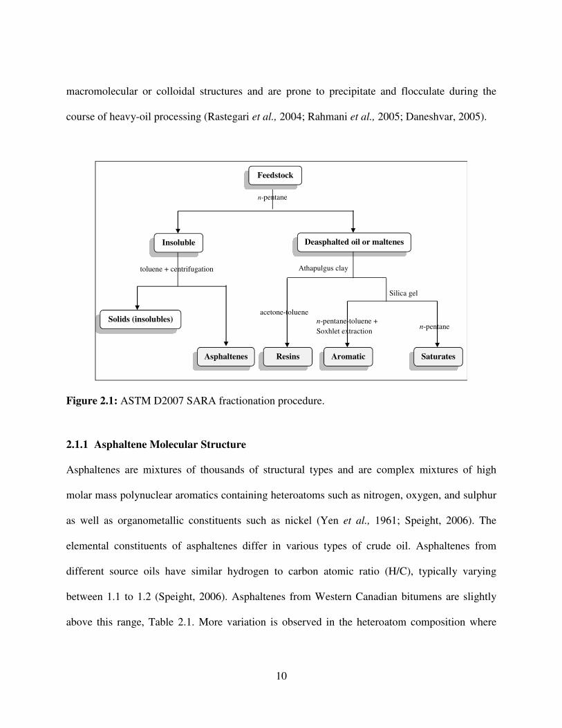
Heavy oils and bitumens are often characterized in terms of SARA fractions (saturates,
aromatics, resins, and asphaltenes). These classes differ based on polarity, solubility, and
adsorptive characteristic as shown in Figure 2.1. Saturates are nonpolar compounds which
include paraffins and cycloparaffins or naphthenes. Aromatics, resins, and asphaltenes are
polyaromatic compounds with heteroatomic species such as nitrogen, oxygen, and sulphur in
their structure. The ring systems in the aromatics vary from mono-aromatics to tri-aromatics.
Resins and asphaltenes contain larger ring systems and are progressively higher in molecular
weight, aromaticity, polarity, and hetero-compound content.
Asphaltenes are by far the most studied and yet the least understood class of crude oil.
Asphaltenes are dark, sticky solids that are defined as the fraction of the oil that is insoluble in
normal alkane solvents, such as n-heptane or n-pentane, but soluble in aromatic solvents such as
toluene or benzene (Yen and Chilingarian, 2000). Asphaltenes self-associate into
10
macromolecular or colloidal structures and are prone to precipitate and flocculate during the
course of heavy-oil processing (Rastegari et al., 2004; Rahmani et al., 2005; Daneshvar, 2005).
Figure 2.1: ASTM D2007 SARA fractionation procedure.
2.1.1 Asphaltene Molecular Structure
Asphaltenes are mixtures of thousands of structural types and are complex mixtures of high
molar mass polynuclear aromatics containing heteroatoms such as nitrogen, oxygen, and sulphur
as well as organometallic constituents such as nickel (Yen et al., 1961; Speight, 2006). The
elemental constituents of asphaltenes differ in various types of crude oil. Asphaltenes from
different source oils have similar hydrogen to carbon atomic ratio (H/C), typically varying
between 1.1 to 1.2 (Speight, 2006). Asphaltenes from Western Canadian bitumens are slightly
above this range, Table 2.1. More variation is observed in the heteroatom composition where
n-pentane
Feedstock
Resins
Insoluble Deasphalted oil or maltenes
Athapulgus clay toluene + centrifugation
Asphaltenes Saturates Aromatic
n-pentane n-pentane-toluene +
Soxhlet extraction
acetone-toluene Solids (insolubles)
Silica gel
11
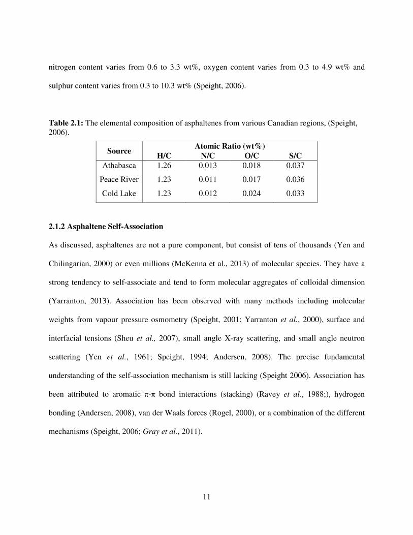
nitrogen content varies from 0.6 to 3.3 wt%, oxygen content varies from 0.3 to 4.9 wt% and
sulphur content varies from 0.3 to 10.3 wt% (Speight, 2006).
Table 2.1: The elemental composition of asphaltenes from various Canadian regions, (Speight,
2006).
Source Atomic Ratio (wt%)
H/C N/C O/C S/C
Athabasca 1.26 0.013 0.018 0.037
Peace River 1.23 0.011 0.017 0.036
Cold Lake 1.23 0.012 0.024 0.033
2.1.2 Asphaltene Self-Association
As discussed, asphaltenes are not a pure component, but consist of tens of thousands (Yen and
Chilingarian, 2000) or even millions (McKenna et al., 2013) of molecular species. They have a
strong tendency to self-associate and tend to form molecular aggregates of colloidal dimension
(Yarranton, 2013). Association has been observed with many methods including molecular
weights from vapour pressure osmometry (Speight, 2001; Yarranton et al., 2000), surface and
interfacial tensions (Sheu et al., 2007), small angle X-ray scattering, and small angle neutron
scattering (Yen et al., 1961; Speight, 1994; Andersen, 2008). The precise fundamental
understanding of the self-association mechanism is still lacking (Speight 2006). Association has
been attributed to aromatic π-π bond interactions (stacking) (Ravey et al., 1988;), hydrogen
bonding (Andersen, 2008), van der Waals forces (Rogel, 2000), or a combination of the different
mechanisms (Speight, 2006; Gray et al., 2011).
12
There are two main concepts of asphaltene nano-aggregates: colloids (Mullins et al., 2012) and
macromolecules (Agrawala and Yarranton, 2001). The colloidal theory postulates that asphaltene
molecules are primarily continental structures each consisting of primarily of a condensed
aromatic sheet. It is hypothesized that these sheets form colloidal stacks held together by π-π
bonds. The stacks are expected to aggregate strongly if exposed but are stabilized as suspended
colloids by resins adsorbed on the surface of the colloid (Yen et al., 1967; Mullins et al., 2007).
A short range intermolecular repulsive force between resins is believed to prevent flocculation of
asphaltene particles. Any change in composition, pressure and temperature can disturb the
equilibrium of the colloidal system leading to desorption of resins and consequently causing
asphaltene precipitation (Mullins et al., 2012). For example, addition of an n-alkane to a crude
oil can desorb resins and re-established equilibrium can be achieved by reduction in the free
surface energy of asphaltene by flocculation (Hemmami et al., 2007). The colloidal model
accounts for asphaltene self-association through the limited aggregation of colloidal particles
upon partial desorption of the resins. The colloidal model is quite complex and requires a large
number of parameters, and cannot explain the effect of solvents like toluene on asphaltene
association and precipitation. The colloidal model predicts that asphaltene precipitation is
irreversible while other studies have proven reversibility of asphaltene precipitations (Hammami
et al., 1999; Hirschberg et al., 1984).
Recent Vapor Pressure Osmometry measurements of asphaltenes in toluene or o-
dichlorobenzene show that asphaltene self-association increases with asphaltene concentration
until a limiting value is reached (Yarranton et al., 2000). The limiting value depends on solvent,
temperature, and pressure. This step-wise aggregation resembles polymerization reactions and
13
therefore asphaltene self-association was modeled analogously to linear polymerization
(Agrawala and Yarranton 2001; Murgich et al., 2002; Merino-Garcia 2004). In this model resins
are not considered a peptizing agent adsorbed on the surface of asphaltene, but are assumed to be
part of polymer-like aggregates, which consist of asphaltene and resin molecules. Aggregates are
held together by dispersion forces rather than covalent forces and behave like macromolecules.
Note, the most successful models for asphaltene association are thermodynamic models which
treat asphaltenes as any other component in a solution. In other words, asphaltenes are implicitly
treated as macromolecules rather than colloids in phase behavior modeling.
2.2 Asphaltene Precipitation
According to field experience (De Boer et al., 1995; Kokal and Sayegh, 1995) and experimental
observations (Fotland et al., 1997; Hammami et al., 2000; Thomas et al., 1992), asphaltenes can
precipitate with a change in conditions, such as the composition, pressure, and temperature of the
crude oil. The most common occurrences of asphaltene precipitation are from depressurized live
conventional oils and from heavy oils diluted with a paraffinic solvent. The effect of composition
and pressure on asphaltene precipitation from conventional oil is generally believed to be
stronger than the effect of temperature. The effect of composition is usually the dominant factor
in precipitation from heavy oil.
At temperatures below approximately 120°C, asphaltenes precipitate as glassy particles of
approximately 1 microns in diameter (Johnston, 2013). These particles tend to flocculate rapidly
into structures up to hundreds of microns in diameter, Figure 2.2. At higher temperatures, they
14
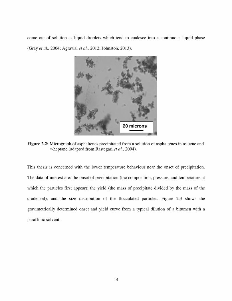
come out of solution as liquid droplets which tend to coalesce into a continuous liquid phase
(Gray et al., 2004; Agrawal et al., 2012; Johnston, 2013).
Figure 2.2: Micrograph of asphaltenes precipitated from a solution of asphaltenes in toluene and
n-heptane (adapted from Rastegari et al., 2004).
This thesis is concerned with the lower temperature behaviour near the onset of precipitation.
The data of interest are: the onset of precipitation (the composition, pressure, and temperature at
which the particles first appear); the yield (the mass of precipitate divided by the mass of the
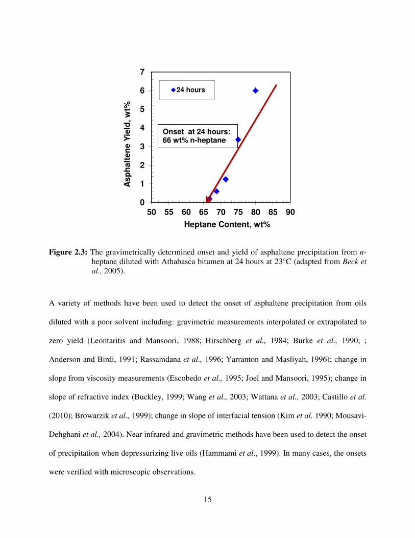
crude oil), and the size distribution of the flocculated particles. Figure 2.3 shows the
gravimetrically determined onset and yield curve from a typical dilution of a bitumen with a
paraffinic solvent.
20 microns
15
Figure 2.3: The gravimetrically determined onset and yield of asphaltene precipitation from n-
heptane diluted with Athabasca bitumen at 24 hours at 23°C (adapted from Beck et
al., 2005).
A variety of methods have been used to detect the onset of asphaltene precipitation from oils
diluted with a poor solvent including: gravimetric measurements interpolated or extrapolated to
zero yield (Leontaritis and Mansoori, 1988; Hirschberg et al., 1984; Burke et al., 1990; ;
Anderson and Birdi, 1991; Rassamdana et al., 1996; Yarranton and Masliyah, 1996); change in
slope from viscosity measurements (Escobedo et al., 1995; Joel and Mansoori, 1995); change in
slope of refractive index (Buckley, 1999; Wang et al., 2003; Wattana et al., 2003; Castillo et al.
(2010); Browarzik et al., 1999); change in slope of interfacial tension (Kim et al. 1990; Mousavi-
Dehghani et al., 2004). Near infrared and gravimetric methods have been used to detect the onset
of precipitation when depressurizing live oils (Hammami et al., 1999). In many cases, the onsets
were verified with microscopic observations.
0
1
2
3
4
5
6
7
50 55 60 65 70 75 80 85 90
As
ph
alt
en
e Y
ield
, w
t%
Heptane Content, wt%
24 hours
Onset at 24 hours:66 wt% n-heptane
16
Caution is required for titration based methods because precipitation does not necessarily reach
detectable levels immediately upon the onset of precipitation. If the solvent injection rate or
depressurization rate is too rapid, more solvent may be injected or lower pressure may be
reached before the onset is detected. Hence, the onset will be reported at too high a solvent
content or too low a pressure. Anderson (1999) recommended a titration rate of 30 mL/30
seconds to avoid overshoot. Similarly, Kraiwattanawong et al. (2007) found that the minimum
light absorbance was did not reflect the true onset and instead use the first deviation in slope in a
plot of absorbance versus volume fraction of solvent to determine the onset point.
For solvent titrations, the solvent content at the onset of precipitation increases with better
solvents because more solvent is required to force precipitation. For n-alkanes, the onset
increases with increasing carbon number up to a carbon number of 10 to 12 and decreases again
higher carbon numbers (Wiehe et al., 2005). Data for the effect of temperature are contradictory
but more show onsets increase with temperature up to 100°C and either reach a plateau or
decreases at higher temperatures (Ali and Al-Ghannam, 1981; Andersen and Birdi, 1990; Hu and
Guo, 1991; Kokal et al., 1992; Andersen, 1994; Andersen et al., 1998; Buenrostro-Gonzalez et
al., 2004; Akbarzadeh et al., 2005). The onset increases slightly with increasing pressure
(Akbarzadeh et al., 2005). For live oils, asphaltenes are more soluble at higher pressure. Lower
onset pressures were observed at higher temperatures indicating that asphaltenes were more
soluble at higher temperatures (Leontaritis and Mansoori, 1988; Hirschberg et al., 1984; Burke et
al., 1990).
17
The same authors show that yield data follow the same trends as the onsets; that is, yields
increase in poorer solvents, decrease with temperature increasing up to 100°C and then stabilize
at higher temperature, and decrease with increasing pressure. With live oils, yield decreases with
increasing pressure above the bubble point. However, below the bubble point, yields decrease
with decreasing pressure as the solution gas evolves from the oil (Tharanivasan et al., 2010).
2.2.1 Asphaltene Precipitation Kinetics
In most of the work presented so far, asphaltenes precipitation was induced by adding the
paraffinic solvent all at once into the crude oil and precipitation data were mostly collected after
approximately 24 hours of equilibration. Relatively little has been reported on the kinetics of
asphaltene precipitation. In general, particle formation involves two kinetic aspects, nucleation
and growth. Nucleation is the formation of a critical nucleus of molecules from a supersaturated
fluid where the free energy minimized by forming a new phase overcomes the cost of forming a
new solid/fluid interface. Once the nucleus is formed, it grows to a larger nano-scale size which
can then coagulate with pre-existing and newly created particles (Zhang et al., 2011). The
growth rate depends on diffusion and adsorption from the medium to the nuclei. Hence, time is
required to reach equilibrium, at least several hours for asphaltenes (Speight, 2006).
Beck et al. (2005) measured asphaltene precipitation over time for various heptane contents
above the onset of precipitation in both air and nitrogen environments. They showed that most of
the precipitation happened within 24 hours in both air and nitrogen atmospheres. After 24 hours,
gradual precipitation continued at a reduced rate for as long as the experiments were conducted
in air, but reached a steady state plateau after 24 hours in a nitrogen environment. The gradual
18
increase in yield after 24 hours in air environment was likely caused by oxidation or oxygen-
catalyzed polymerization. As part of their sample preparation, they aerated their bitumen
samples.
Angle et al. (2006) used optical microscopy to show that onset of asphaltene precipitation as a
function of time and precipitant concentration. They concluded that the onset of asphaltene
precipitation was slow and could take a few hours. They observed a decrease in the lag time prior
to precipitation with an increasing dilution ratio. The appearance of precipitation was sequenced
as spots, strings, clusters and large flocs. However, in their experiments, crude oil was diluted
with 90% toluene. Therefore delay in the precipitation could also be due to the high amount of
toluene added.
Maqbool et al. (2009) studied the onset of asphaltene precipitation of two crude oils using n-
heptane as the precipitant in an air atmosphere. They detected the onset of precipitation using
optical microscopy. Precipitation onset time was defined as the time required for the first
appearance of asphaltene particles. They concluded that the onset of precipitation was a function
of time, varied from a few minutes to several months depending on the precipitant concentration.
Further, no single concentration could be identified as the critical precipitant concentration for
asphaltene precipitation. Near the onset condition, the kinetics of asphaltene precipitation were
very slow but above the onset point, the kinetics were fast and precipitation reached a plateau
within a short time frame.
19
The same authors also investigated the effect of temperature on the kinetics of asphaltene
precipitation upon addition of n-heptane. At higher temperatures, the precipitation onset time
was shorter at a given dilution and the solubility of asphaltenes (Hu and Guo, 2001) was higher.
They speculated that the reduced viscosity and greater diffusivity at higher temperatures led to a
higher aggregation rate and shorter onset time. They remarked that expansion of hydrocarbons,
oxidation of crude oil, and the loss of light hydrocarbons due to evaporation at elevated
temperatures had very little effect on the asphaltene precipitation kinetics. However, they did not
verify their results in an anaerobic environment.
Oxygen can have a significant effect on asphaltene precipitation. Taylor and Frankenfeld (1978)
investigated the effect of oxygen and nitrogen on deposit formation from deoxygenated
hydrocarbons. They proposed that free radical chain reactions involving molecular oxygen
created high molar mass hydrocarbons that fall into the asphaltene solubility class. Watkins et al.
(1996) demonstrated that oxygen dissolved in a liquid hydrocarbon formed polymeric peroxides
through autocatalytic reactions. The peroxides underwent subsequent decomposition reactions
and free radical reactions with hydrocarbons. This reaction led to new asphaltene formation and
contributed to organic fouling. Beck et al. (2002) examined the effect of pre-treatment of
bitumen samples with oxygen over a range of heptane to bitumen ratios at three temperatures.
They observed no increase in yield at 23oC between the treated and untreated samples, mainly
due to the high viscosity of the bitumen samples which prevented effective aeration. However a
significant increase in yield was observed after aeration at 40 and 70oC.
20
2.3 Asphaltene Flocculation
As noted previously, there are two views on asphaltene precipitation: 1) colloidally dispersed
asphaltene nano-aggregates destabilize and form larger and larger aggregates that eventually
physically separate; 2) asphaltenes chemically separate (precipitate) as micrometer-scale
particles. Measurements below the onset of asphaltene precipitation in heptane-toluene mixtures
have been interpreted as slow aggregation from nanometer to micrometer scale (Angle et al.,
2006; Maqbool et al., 2009). Similarly, Mason and Lin (2003) used time-resolved small angle
neutron scattering to investigate the kinetics of asphaltene nanoparticle aggregation in an
asphaltene rich crude oil mixed with a paraffinic British crude oil. Their results indicated an
initial particle diameter in the nanometre scale with growth to the micrometre range over a
period of 11 days. They used a diffusion limited aggregation model to define a “characteristic
time” to show when the asphaltene flocs first appeared. However, there are no conclusive
observations of particles in the intermediate size range between nanometer-scale
colloids/macromolecules and micrometer scale particles. In most cases, once a supersaturation
condition is reached, the transition from nanometer to micrometer scale appears to be
instantaneous. It is more likely that asphaltenes precipitate as micrometer-scale particles and
these authors are observing the outcome of a nucleation and growth process (possibly with
oxygen artifacts) rather than an aggregation process.
There are many examples of instantaneous particle formation. Ferworn et al. (1993) concluded
that asphaltene particle growth and flocculation from n-heptane crude oils is an instantaneous
process; that is the agglomerates reached a critical size within a few seconds and the asphaltene
particles size distribution remained constant over time. Ostlund et al. (2002) used nuclear
21
magnetic resonance to study the kinetics of flocculation of asphaltene. They also found a
dramatic increase in flocculation above a certain “threshold concentration,” which could be
referred as the onset point of the precipitation. Rastegari et al. (2004) and Daneshvar (2005) also
observed instantaneous particle formation at the onset of precipitation. This review will focus on
the asphaltene flocculation from micrometer-scale primary particles.
2.3.1 Floc Structure and Fractal Dimension
The shape and structure of asphaltene flocs in various solvents have been investigated using a
variety of techniques including small-angle neutron and X-ray scattering (Savvidis et al., 2001;
Mason and Lin, 2003; Headen et al., 2009; Eyssautier, 2011), a combination of viscosimetric and
neutron scattering measurement (Sheu, 1998; Fenistein et al.,199; Hoepfner et al., 2013), optical
microscopy (Rahmani et al., 2005), and particle size analyzer (Rastegari et al., 2004; Daneshvar
2005). These investigations have concluded that precipitated asphaltenes form fractal clusters.
The nature of fractals will be discussed later.
Savvidis et al. (2001) found that the precipitated and dried asphaltenes appeared as dense
spherical structures with diameters ranging from nanometers to micrometers. However,
asphaltene particles still suspended in solvent form loose fractal-like structures. Sheu (1998)
determined the fractal dimension based on a series of time dependent viscosity measurements of
asphaltene flocs in the mixture of 75 wt% heptane to 25 wt% toluene (with no agitation). He
assumed that the asphaltene flocs were hydrodynamically spherical and were influenced by
diffusion-limited aggregation. He found that the fractal dimension of the asphaltene flocs varied
from 1.49 to 1.8 for different asphaltenes and concentrations. The asphaltene fractal dimension
22
decreased as the concentration increased. A restructuring effect was also observed when the
flocculated asphaltenes were shaken for one minute; the fractal dimension increased from 1.53 to
1.8, resulting in a denser structure.
Rastegari et al. (2004) and Daneshvar (2005) found that asphaltene flocs were loose fractal-like
structures rather than spherical aggregates. They determined fractal dimension by image analysis
and indirectly from calculation of the mass of precipitated asphaltenes measured by particle size
analysis and then compared it to the fraction precipitated gravimetrically. Rastegari et al. (2004)
estimated a fractal value of 1.6 for asphaltenes flocs in a mixture of 60:40 n-heptane:toluene.
Daneshvar (2005) calculated volume fractions occupied by flocs assuming fractal dimensions for
bitumen diluted with heptane at 93.5 wt% n-heptane. Based on visual observations of settled
asphaltenes at high dilution ratios, he concluded that the flocculated asphaltenes occupied no
more than 30 to 40 vol% of the solution volume and that the fractal dimension must be larger
than 2.0. He used a fractal dimension of 2.05 for his modeling.
Rahmani et al. (2005) employed a photographic technique coupled with image analysis to
measure the size and fractal dimension of asphaltene aggregates formed in n-heptane–toluene
mixtures. They determined terminal settling velocities and characteristic aggregate lengths to
estimate the two- and three-dimensional fractal dimensions, estimated to be 1.06 to 1.40
depending on the shear rate and asphaltene concentration in heptane-toluene solvent mixtures.
These small fractal dimensions showed that asphaltene flocs loose, highly porous structures.

23
2.3.2 Factors Affecting Asphaltene Flocculation
Asphaltene floc size distributions and fractal behaviour have been investigated as a function of
composition, temperature, pressure, and shear using a variety of techniques including laser
particle size analysis (Ferworn et al., 1993; Rastegari et al., 2004; Daneshvar, 2005), small-angle
neutron and X-ray scattering (Savvidis et al., 2001; Mason and Lin, 2003; Headen et al., 2009;
Eyssautier, 2011), and optical microscopy and image analysis (Rahmani et al., 2005).
Composition
Composition is an important parameter in determining the size and rate of asphaltene
flocculation. Ferworn et al. (1993) used a particle size analyzer to investigate asphaltene floc
growth over 24 hours for six different crude oils diluted with n-heptane and in some cases with
n-hexadecane and n-pentane. They observed lognormal distributions in all cases with floc sizes
ranging from tens to hundreds of micrometers. The mean floc size increased as the diluent to
bitumen ratio increased (making the medium a poorer solvent) and as the carbon number of the
n-alkane decreased (lower carbon number n-alkanes are poorer solvents). They also investigated
the effect of oxygen on the particle size and performed tests under a nitrogen blanket. They
observed no measurable differences between the asphaltenes mean floc sizes in air versus
nitrogen.
Nielsen et al. (1994) used a similar technique, and found the mean size of asphaltene flocs
ranged from 266 to 495 µm for different oils diluted with n-pentane. They observed bimodal size
distributions of asphaltene flocs. However, most other investigators have observed only
unimodal distributions.
24
Rastegari et al. (2004) used a particle size analyzer to measure the asphaltenes particle size
distribution in a series of n-heptane-toluene mixtures. The particle size distributions were
observed to be lognormal. The volume mean diameters ranged up to 400 µm with an individual
particle diameter of approximately 1 µm. They found that asphaltene floc size increased as the
asphaltene concentration and n-heptane content increased. Higher concentration is expected to
cause more particle collisions and therefore greater flocculation rate. Adding n-heptane makes
the medium a poorer solvent for asphaltenes increasing the driving force for flocculation.
According to their experiments, asphaltene flocs reached a steady-state size distribution
indicating that flocculation does not continue indefinitely. To achieve a steady-state condition,
flocculation must eventually be balanced by disintegration. Hence, asphaltene flocculation
appears to be a reversible process.
Daneshvar (2005) studied the asphaltene flocculation in diluted bitumen systems with n-heptane
and n-pentane using a particle size analyzer. He observed that the volume mean diameter
increased as the dilution ratio increased from 75 to 93.5 wt% n-heptane in bitumen but remained
constant at higher dilutions. At low to moderate heptane content, they observed an increase in the
number and size of the asphaltene flocs, resulting in higher flocculation rate as the heptane
content increased. At higher heptane content, further dilution had little effect on floc size, and the
number concentration of the flocs decreased as the system becomes more dilute. He also found
that the type of diluent such as n-pentane led to significantly more flocculation both initially and
at steady state. The steady state volume mean diameter was approximately 290 µm in n-pentane
compared to 100 µm in n-heptane. Maqbool et al. (2011) also observed larger mean diameters at
higher n-heptane contents. Maqbool et al. (2011) found that as the heptane concentration
25
increased, the particle size distribution of asphaltene aggregates shifted more quickly to larger
diameters.
Kraiwattanawong et al. (2009) investigated the effect of asphaltene dispersants on aggregate size
distribution using a paraffinic solvent like n-heptane. Their study showed that large asphaltene
particles are in fact aggregates consisting of very small (sub-micrometer) size asphaltene
particles. Their result showed a bimodal distribution, indicating that two types of asphaltenes
exist. The asphaltenes in the size range of 0.1-1 µm were called “stabilized asphaltenes. Once
asphaltenes are destabilized, they form an intermediate phase called colloidal asphaltenes, which
grow to a size of about 1-30 µm in diluted mixture. These asphaltenes with the size greater than 1
µm were called flocculated asphaltene.
Najafi et al. (2011) studied the kinetics of asphaltene flocculation of several crude oil samples
exposed to ultrasonic waves at different time intervals and used confocal microscopy to observe
the size distribution in a mixture of n-pentane and toluene. The size distribution of asphaltene
flocs ranged from 1 to 10 µm after 120 minutes, showing a multimodal distribution. They
concluded that ultrasound reduced the formation of macrostructure aggregates.
Pressure and Temperature
The effect of pressure or temperature on asphaltene floc size distribution has been investigated
by Nielsen et al. (1994) and Daneshvar (2005). Nielsen et al. (1994) studied the effect of
pressure and temperature of crude oil diluted with n-pentane. They found that the mean floc size
26
increased slightly as pressure increased and the temperature had negligible effect on asphaltene
flocculation.
Daneshvar (2005) investigated the effect of temperature on the volume mean diameter and
number count rate for n-heptane dilution of 93.5 wt%, at three different mixing speeds. At the
slowest mixing speed of 195 rpm, the volume mean diameter did not notably change as
temperature increased, but the number count rate decreased. At the higher mixing speeds, the
volume mean diameter and number count rate reached a maximum at a temperature of
approximately 45°C. The observations were surprising because, in the temperature range of these
experiments, asphaltene yield decreases as temperature increases and; therefore, the number of
individual particles decreases at a given dilution ratio. The number of flocs and mean floc size
are both expected to decrease as the number of particles decreases in contrast to the observations.
Daneshvar speculated that the increase in volume mean diameter as temperature increased up to
40°C was due to the stickiness of asphaltene flocs. The decrease in volume means diameter and
number count at higher temperatures could be result of deposition on the mixer and beaker walls
or of the formation of more compact flocs with higher fractal dimension.
Shear
Rastegari et al. (2004) and Daneshvar (2005) both investigated the effect of mixing rate on the
asphaltene floc size. They found that asphaltene flocculation is reversible. At higher mixing
rates, asphaltene flocs disintegrated and steady state particle size distributions were reached
faster. The shape of the sheared particle size distributions indicated that shattering is the
dominant disintegration mechanism.
27
2.4 Asphaltene Flocculation Modeling
2.4.1 Flocculation Models in General
As noted previously, asphaltenes precipitate as micron sized particles that flocculate into
structures up to hundreds of micron in diameter. In this thesis, it is assumed that the micron
diameter particles are the final product of a phase change. Note, some other models assume
flocculation begins with nano-aggregates possibly with a second level of aggregation occurring
once micron scale flocs form (Mullins et al., 2012; Maqbool et al., 2011).
Flocculation refers to the formation of clusters in colloidal suspension systems. Individual
particles dispersed in the liquid phase will stick to each other and form irregular particle clusters,
flocs, or aggregates. Research in flocculation has spanned many fields, such as biomedicine,
biotechnology, polymer physics, and surface chemistry. In processes concerned with fine
particles, it is often the floc that is the important unit rather than an individual particle, and the
size and the shape of the flocs control the behaviour of the systems. One method that attempts to
describe the geometry of the flocs is by simulating the random aggregation and to date two
mechanisms have been presented as a basis for such simulations; particle-cluster and cluster-
cluster flocculation.
In particle-cluster flocculation, the floc is formed through successive addition of single particles
of unit radius which approach along a linear trajectory, randomly distributed in space while the
particle is being rigidly fixed at their first point of contact. In cluster-cluster flocculation, the
collisions between small clusters are included. Each collision is calculated by randomly rotating
the colliding clusters and moving one along a randomly chosen linear trajectory until collision
28
occurs. The clusters are considered rigidly-fixed at their first point of contact (Sutherland, 1967;
Sutherland and Goodarz-Nia, 1971).
In either case, the asphaltene flocculation is modeled based on a population balance of the
individual particles. The choice of the population balance equation depends on whether the
flocculation is irreversible or reversible of which both will be discussed in the next sections.
Many models only consider irreversible asphaltene flocculation and are not applicable for the
systems in which asphaltene disintegration occurs. Asphaltene flocculation systems are shear
sensitive and reversible. The reaction kernels for cluster-cluster flocculation are only considered
in this thesis. The approach is the same for particle-cluster flocculation except that the interacting
species must be a single particle. The population balance equations are reviewed below.
2.4.2 Irreversible Flocculation
Irreversible flocculation refers to the collision of particles i and j that stick together to form a
larger cluster, k, and no allowance is made for break-up of aggregates as follows:
�� +�� �(�,�) →�� i+j=k (2.2)
where Fi,j represents the flocculation reaction rate between Mi and Mj. This reaction kernel
depends on a number of factors such as particle size and transport mechanism. Mi, and Mj are
clusters containing i and j elementary units. Smoluchowski assumed that the particle collisions
were binary, the fluctuations in density were relatively small, and only random collisions
occurred. The classical irreversible Smoluchowski (1916) population balance equation represents
29
the rate of change of concentration of kth
aggregates and is given by:
� ��� = �
�∑ F��C������������→� C� − C� ∑ F��C�⋈��� (2.3)
where Fi,j, and Fik are the reaction kernels representing the number of reactions per unit volume
per unit time which result in flocculation. Ci and Cj are concentrations of species i and j, and t is
time. The first term on the right hand side represents the rate of formation of k aggregates by
collision of any pair of aggregates, i and j forming i+j=k. Because of the summation, each
collision is counted twice; therefore the factor ½ is included. The second term accounts for the
loss of k aggregates by collision and aggregation with any other aggregates (Elimelech et al.,
1998).
The rate of collision between particles is determined by transport mechanisms such as Brownian
diffusion and inter-particle interactions such as London dispersion forces. For two particles to
aggregate, these two particles must first be brought into close proximity by a transport
mechanism. Transport mechanisms give neighboring particles different velocities and cause
collisions. Whether or not the particles are attached to each other after a collision depends on the
net inter-particle forces. The differences in the velocities of neighboring particles may result
from Brownian motion, spatial velocity variations within the fluid (i.e., fluid shear), and
sedimentation (i.e., differential settling). Brownian motion is usually important when the
particles are of submicron size. However, as the particles grow larger, Brownian aggregation
becomes less important and differential settling becomes the dominant mechanism.
30
The Smoluchowski (1916) population balance equation was initially derived assuming Brownian
motion was the only transport mechanism, and particle diffusion coefficients were constants.
Assuming the Stokes-Einstein relation holds for the diffusion coefficient, Fi,j, Brownian
coagulation was expressed as shown in Equation 2.4 (Higashitani et al.,1992):
"#,$ = 2&'3) *+#1/3 + +$1/3. / 1
+#1/3+ 1+$1/30 (2.4)
where K is Boltzmann’s constant, T is the absolute temperature, µ is the viscosity of the
suspending fluid, and vi and vj are the volumes of particles i and j.
The origin of these forces is the attraction between a temporary dipole and the corresponding
induced dipoles (London theory) between the particles. Higashitani et al. (1979) proposed a
modified Smoluchowski equation. The modification considered the hydrodynamic interactions
and the van der Waals potential as follows (Higashitani and Matsuno, 1979; Friedlander, 2000):
"#,$= 2&'3)1#,$ *+#1/3 + +$1/3. / 1
+#1/3+ 1+$1/30 (2.5)
This model was consistent with the experimental data from the flocculation of polystyrene latex
particles (Higashitani et al., 1992) .
Ball et al. (1987) modeled the Smoluchowski equations using reaction-limited cluster
aggregation theory. They determined the reaction kernel by cluster fractal geometry:
for (2.7.a.) Fi, j ~ Mλ /D f , M i ≈ M j = M
31
for (2.7.b)
where λ is the adjustable parameter and Df is the fractal dimension. Equation 2.7 was developed
for low concentrations where three-cluster effects could be ignored.
Rastegari et al. (2004) modified this reaction-limited cluster-cluster aggregation reaction kernel
to obtain the following general equation:
(2.8)
where k′f is the reaction constant, Df is the fractal dimension of the flocs. Since the mass of a floc
is directly proportional to the number of particles in the floc, Daneshvar (2005) modified it as
follows:
(2.9)
Equation 2.9 is the flocculation rate term that will be used in this thesis.
2.4.3 Reversible Flocculation
Reversible flocculation refers primarily to the flocculation and separation of flocs under shear.
Reversible flocculation happens mostly for flocs that are held together by van der Waals forces.
In these systems, flocculation and disintegration both affect the floc distributions. The
flocculation rate decreases the number of clusters while the disintegration rate increases it and
steady state particle size distribution is observed. The Smoluchowski population balance
Fi, j ~ M i
1/D f M j
λ /D f , M i >> M j
λ
++
+′= ff D
j
ji
iD
i
ji
j
fji MMM
MM
MM
MkF
/1/1
,
λ
++
+= ff D
j
ji
iD
i
ji
j
fji nnn
nn
nn
nkF
/1/1
,
32
equation for the kth
species, including flocs, up to the order of N for irreversible flocculation
(Family et al., 1986) is given by:
(2.11)
(2.12)
where D(i,j) is the disintegration reaction term representing the number of reactions per unit
volume per unit time. Disintegration involves large particles breaking into a number of smaller
particles through grinding or shattering. The disintegration reaction term is a function of the
particle diameter and is usually represented as a power law. Welt et al. (1977), and Rastegari et
al. (2004) employed the following disintegration reaction term for a floc of radius Ri :
2� = &3(4�)5 (2.13)
where Kd is the disintegration reaction constant and the power of β varies within the range of 0 to
3.
Rastegari et al. (2004) expanded Equation 2.13 to represent the mass of a floc of size Ri+j that
breaks into flocs of size Ri and Rj, as follows:
(2.14)
where i and j represent the two flocs formed when a larger floc breaks up, Kd is the disintegration
reaction constant, Ri, Rj, are the radii of the flocs, Df is the mass (number) fractal dimension of
the flocs, and the disintegration reaction exponent β is a number from 0 to 3. Equation 2.14 was
M i + M j
F (i, j ) →
D(i, j )←
M i+ j
dCk
dt=
1
2Fi, jCiC j − Di+ jCi+ j( ) − Fk, jCkC j − Di+ jCi+ j( )
j=1
N−k
∑i+ j=k i=1
k−1
∑
D i, j( ) = Kd Ri+ j
β = Kd M i
1/D f + M j
1/D f( )β
33
developed for low concentrations. Since the mass of a floc is directly proportional to the number
of particles in the floc, Daneshvar (2005) modified Equation 2.14 as follows:
(2.15)
Equation 2.15 is the disintegration reaction term that will be used in this thesis.
2.4.4 Asphaltene Flocculation Models
Most researchers have worked with well mixed systems and therefore have considered
asphaltene flocculation as a reaction controlled (low probability of sticking after collision) rather
than diffusion controlled (low probability of collision) process. The kinetics of asphaltene
flocculation based on the viscosity of asphaltene flocs with time in a heptane/toluene mixture
was investigated by Sheu (1998). He observed that initially the viscosity decreased and then
stayed constant. After 90 minutes, the viscosity started increasing as a result of asphaltene
flocculation. The flocculation rate was very slow initially but increased exponentially as the floc
size increased. He interpreted the trends as reaction limited flocculation, where the flocculation
rate increased as the size of the flocs increased.
Najafi et al. (2011) studied the kinetics of asphaltene flocculation of several crude oil samples
for different time intervals from the addition of n-pentane to crude oil in toluene. They showed
that in the first 90 minutes, the size of the aggregates increased rapidly, matching well with a
reaction-limited aggregation model. After 90 minutes, the size of the aggregate continued to
increase at a reduced rate.
( )βff D
j
D
idji nnkD/1/1
+=+
34
Rastegari et al. (2004) studied the kinetics of asphaltene particle growth in model systems of
asphaltenes, n-heptane, and toluene using a particle size analyzer. Asphaltene flocs reached a
steady-state size distribution, indicating that flocculation does not continue indefinitely but is
balanced by disintegration. They developed a reversible reaction limited flocculation model that
successfully fit the particle-size distributions and growth in mean volume diameter over time.
They examined disintegration through erosion and shattering mechanisms. Erosion is the
removal of individual or primary particles from flocs through grinding or shear. Shattering is the
fragmentation of flocs into smaller flocs of any size less than the original floc. They concluded
that shattering was the dominant disintegration mechanism.
In a similar way, Rahmani et al. (2004) developed a mathematical model based on population
balance to analyze reversible experimental data for asphaltene floc size distribution for a solution
of asphaltene in n-heptane-toluene mixture as the solvent. The aggregation behavior of
asphaltenes was investigated by monitoring the size distribution of flocs for various shear rates,
n-heptane to toluene ratios, and asphaltene concentrations. They found that steady-state
condition was reached when the fragmentation rate balances the aggregation rate and the floc
size distribution no longer changes with time. In their modeling, they included collision
efficiency, collision frequency, fragmentation rate, breakup distribution function, and porosity
instead of fractal dimension. Collision frequency solely due to the fluid shear was employed in
their modeling. Furthermore, it was assumed that the collision efficiency is equal to one. They
used a simple correlation to estimate the breakup rate as a function of floc apparent volume and
shear rate. They found a correlation between porosity, as an adjustable parameter, and shear rate.
35
Daneshvar (2005) developed a flocculation model based on population balance to analyze
reversible experimental data for asphaltene floc size distribution in diluted bitumen systems. To
minimize the computational time, his population balance was based on clusters of particles rather
than individual particles. He investigated the effect of shear rate, dilution ratio and temperature
on the model parameters. The effect of changing the dilution ratio was matched by adjusting only
the reaction rate constants. The effect of shear rate was matched by adjusting the fractal
dimension. The volume mean diameters were well matched; however the predicted trends for the
number mean diameter and number counts versus time were far from the experimental data.
They used a fractal dimension of 2.05. In this case, the apparent volume of the asphaltene flocs
in the mixture was 33% of the total volume.
36
CHAPTER THREE: EXPERIMENTAL METHODS
In this chapter, the experimental procedures used to measure the kinetics of asphaltene
precipitation and flocculation of diluted bitumen systems are described in detail including
asphaltene extraction, asphaltene precipitation yield and onset measurements, flocculation
experiments, and particle size analysis.
3.1 Materials
A Western Canadian bitumen (WC_B2), already treated to remove water and solids, such as sand
and clays, was supplied by Shell Canada Ltd. The residual water content was measured by Karl
Fischer analysis and was less than 1 wt%. Toluene and n-heptane were obtained from VWR
International LLC. and were 99% pure. Nitrogen was 99.99% pure and was purchased through
Praxair.
The saturate, aromatic, resin, and asphaltene composition of the bitumen was determined
elsewhere (Okafor, 2014) using the ASTM D2007M procedure, Table 3.1. The SARA procedure
used n-pentane to precipitate the asphaltenes. However, in this thesis, most experiments were
conducted with n-heptane (n-C7) precipitated asphaltenes. Asphaltenes precipitated with n-
pentane and n-heptane are termed “C5-asphaltenes” and “C7-asphaltenes”, respectively. Both
values are reported in Table 3.1. The density of the bitumen used in this study was also measured
by Okafor with an Anton Paar density meter and was 1153.5 kg/m3 at 20°C. The viscosity of the
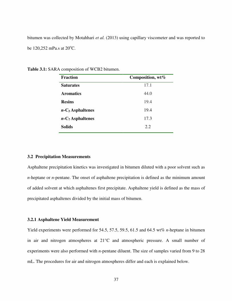
37
bitumen was collected by Motahhari et al. (2013) using capillary viscometer and was reported to
be 120,252 mPa.s at 20oC.
Table 3.1: SARA composition of WCB2 bitumen.
Fraction Composition, wt%
Saturates 17.1
Aromatics 44.0
Resins 19.4
n-C5 Asphaltenes 19.4
n-C7 Asphaltenes 17.3
Solids 2.2
3.2 Precipitation Measurements
Asphaltene precipitation kinetics was investigated in bitumen diluted with a poor solvent such as
n-heptane or n-pentane. The onset of asphaltene precipitation is defined as the minimum amount
of added solvent at which asphaltenes first precipitate. Asphaltene yield is defined as the mass of
precipitated asphaltenes divided by the initial mass of bitumen.
3.2.1 Asphaltene Yield Measurement
Yield experiments were performed for 54.5, 57.5, 59.5, 61.5 and 64.5 wt% n-heptane in bitumen
in air and nitrogen atmospheres at 21°C and atmospheric pressure. A small number of
experiments were also performed with n-pentane diluent. The size of samples varied from 9 to 28
mL. The procedures for air and nitrogen atmospheres differ and each is explained below.
38
Air Atmosphere
Diluted bitumen samples were prepared by adding a known mass of bitumen to a clean 30 mL
centrifuge tube. A specified mass of n-heptane was then added to achieve the desired weight
percent of solvent. The n-heptane was added at a rate of approximately 1 mL/minute while
keeping the mixture well stirred using a magnetic bar and stirrer. The mixtures were then
sonicated for 50 minutes and left to settle for the desired time. Then, the samples were
centrifuged using a Hettich Model EBA 12 centrifuge for five minutes at 4000 rpm. The
supernatant was decanted and filtered through a glass microfiber filter with VWR grade of 696.
The remaining sediment (precipitated asphaltenes and entrained continuous phase) were washed
with 20 mL of n-heptane and the mixture was sonicated for 15 minutes and centrifuged for five
minutes at 4000 rpm. The washing step was repeated for a total of two washings. The
precipitated material was dried in a Thermo Scientific Labline vacuum oven at 60oC at -70 kPA
until no further change in the mass was detected. Note, time zero is defined as the time at which
the last drop of solvent was added to the bitumen.
The precipitate contains both asphaltenes and inorganic solids which co-precipitate with the
asphaltenes. To obtain the solids content, the precipitate was dissolved in toluene and sonicated
for one hour and centrifuged at 3500 rpm for six minutes. The supernatant was decanted. This
procedure was repeated until the toluene solution was colorless. The remaining solids were dried
and weighed. Asphaltene precipitation yields were calculated as the mass of precipitate less the
mass of solids all divided by the initial mass of bitumen; that is, the asphaltene yields were all
determined on a solids-free basis. The repeatability of the yields was ±6%.
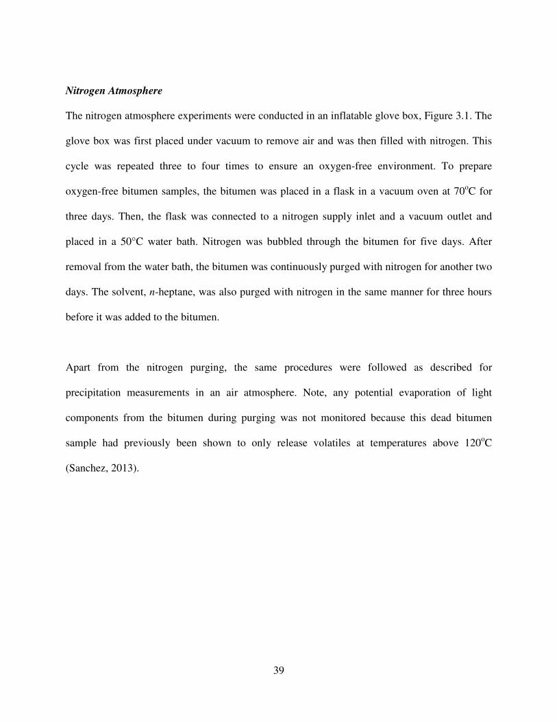
39
Nitrogen Atmosphere
The nitrogen atmosphere experiments were conducted in an inflatable glove box, Figure 3.1. The
glove box was first placed under vacuum to remove air and was then filled with nitrogen. This
cycle was repeated three to four times to ensure an oxygen-free environment. To prepare
oxygen-free bitumen samples, the bitumen was placed in a flask in a vacuum oven at 70oC for
three days. Then, the flask was connected to a nitrogen supply inlet and a vacuum outlet and
placed in a 50°C water bath. Nitrogen was bubbled through the bitumen for five days. After
removal from the water bath, the bitumen was continuously purged with nitrogen for another two
days. The solvent, n-heptane, was also purged with nitrogen in the same manner for three hours
before it was added to the bitumen.
Apart from the nitrogen purging, the same procedures were followed as described for
precipitation measurements in an air atmosphere. Note, any potential evaporation of light
components from the bitumen during purging was not monitored because this dead bitumen
sample had previously been shown to only release volatiles at temperatures above 120oC
(Sanchez, 2013).
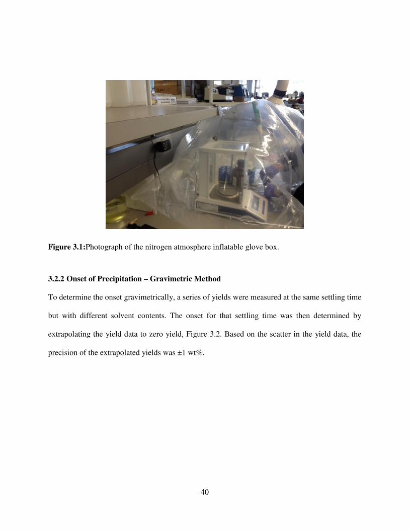
40
Figure 3.1:Photograph of the nitrogen atmosphere inflatable glove box.
3.2.2 Onset of Precipitation – Gravimetric Method
To determine the onset gravimetrically, a series of yields were measured at the same settling time
but with different solvent contents. The onset for that settling time was then determined by
extrapolating the yield data to zero yield, Figure 3.2. Based on the scatter in the yield data, the
precision of the extrapolated yields was ±1 wt%.
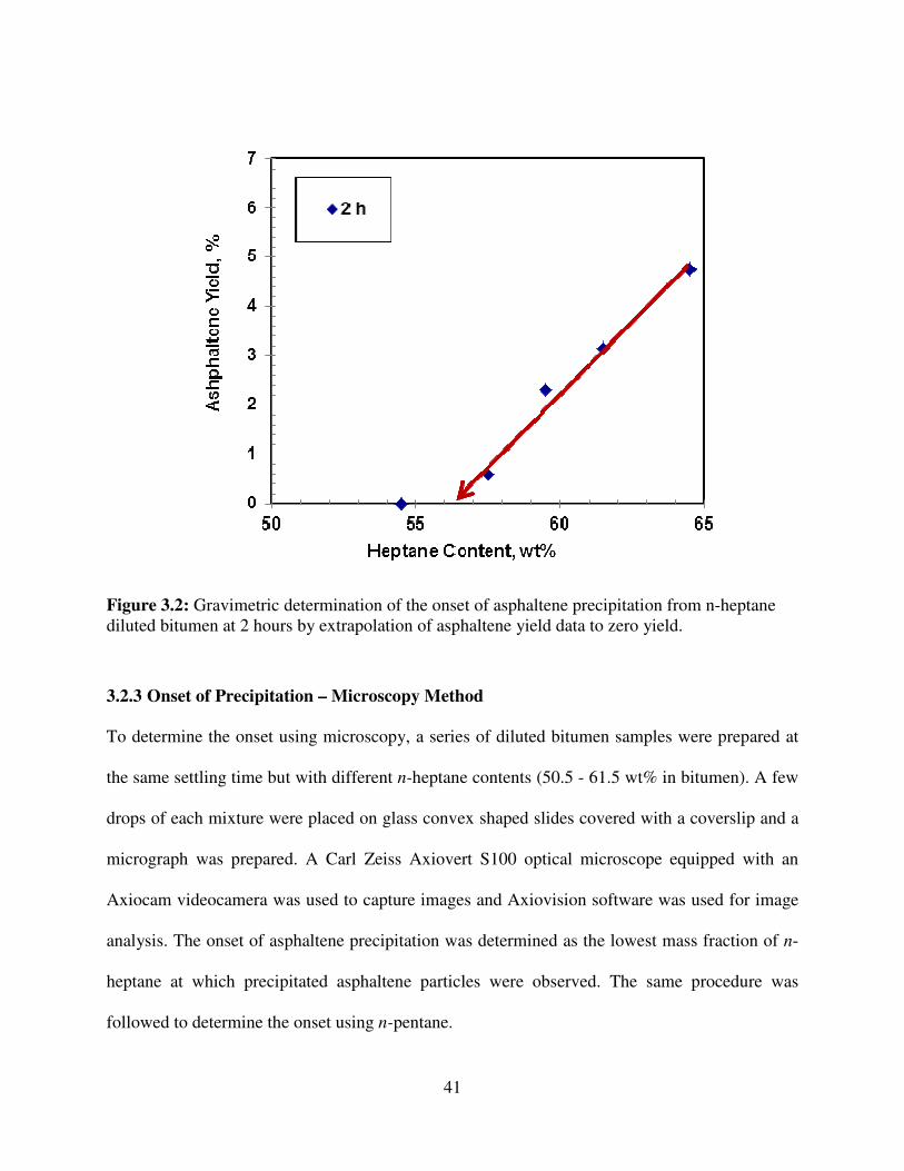
41
Figure 3.2: Gravimetric determination of the onset of asphaltene precipitation from n-heptane
diluted bitumen at 2 hours by extrapolation of asphaltene yield data to zero yield.
3.2.3 Onset of Precipitation – Microscopy Method
To determine the onset using microscopy, a series of diluted bitumen samples were prepared at
the same settling time but with different n-heptane contents (50.5 - 61.5 wt% in bitumen). A few
drops of each mixture were placed on glass convex shaped slides covered with a coverslip and a
micrograph was prepared. A Carl Zeiss Axiovert S100 optical microscope equipped with an
Axiocam videocamera was used to capture images and Axiovision software was used for image
analysis. The onset of asphaltene precipitation was determined as the lowest mass fraction of n-
heptane at which precipitated asphaltene particles were observed. The same procedure was
followed to determine the onset using n-pentane.
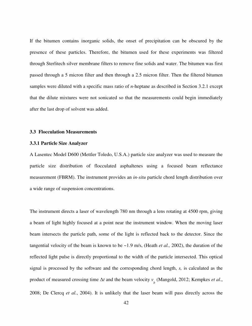
42
If the bitumen contains inorganic solids, the onset of precipitation can be obscured by the
presence of these particles. Therefore, the bitumen used for these experiments was filtered
through Sterlitech silver membrane filters to remove fine solids and water. The bitumen was first
passed through a 5 micron filter and then through a 2.5 micron filter. Then the filtered bitumen
samples were diluted with a specific mass ratio of n-heptane as described in Section 3.2.1 except
that the dilute mixtures were not sonicated so that the measurements could begin immediately
after the last drop of solvent was added.
3.3 Flocculation Measurements
3.3.1 Particle Size Analyzer
A Lasentec Model D600 (Mettler Toledo, U.S.A.) particle size analyzer was used to measure the
particle size distribution of flocculated asphaltenes using a focused beam reflectance
measurement (FBRM). The instrument provides an in-situ particle chord length distribution over
a wide range of suspension concentrations.
The instrument directs a laser of wavelength 780 nm through a lens rotating at 4500 rpm, giving
a beam of light highly focused at a point near the instrument window. When the moving laser
beam intersects the particle path, some of the light is reflected back to the detector. Since the
tangential velocity of the beam is known to be ~1.9 m/s, (Heath et al., 2002), the duration of the
reflected light pulse is directly proportional to the width of the particle intersected. This optical
signal is processed by the software and the corresponding chord length, s, is calculated as the
product of measured crossing time ∆t and the beam velocity vb (Mangold, 2012; Kempkes et al.,
2008; De Clercq et al., 2004). It is unlikely that the laser beam will pass directly across the
43
center of the particle (i.e., its diameter), therefore the chord length is measured. Thousands of
chords are measured which results in producing a robust chord length distribution. The chord
length distribution represents the particle population of the system (Sathe et al., 2010).
The particle size analyzer also records the number of counts per second. Total particle number is
helpful for mass balances and estimating the aggregate porosity (or fractal dimension). However,
the total focused beam reflectance measurement count does not correlate well with the actual
number of flocs or the precipitate fraction in the mixture (Heath et al. 2002; Barrett and Glennon
1999). The instrument can only count one particle or floc at a time. In other words, between
particles or flocs, the reflected time must return to zero for a short time period, therefore, the
dead time will be larger in comparison to the time spent traversing the particles. Hence at
relatively high particle concentration, the instrument dead-time increases and the chances of
particles overlapping in the viewing zone likely increases as well. In addition, the precipitated
asphaltenes are prone to adhere onto the probe window and the impeller, which results in an
erroneous increase in the count rate. The number and volume frequency plots are assumed to be
correct because they deal with the relative number of flocs with specific sizes or volumes.
Instrument Preparation, Calibration and Accuracy Check
Some adjustments, such as discrimination electronics (fine vs. coarse electronics), measurement
duration, and channelling configuration must be set in the FBRM Control Interface (Version 6)
software before any measurements are made.
44
The instrument data processing is adjusted to use either F-(fine) or C-(coarse) discrimination
electronics. The differences are in the interpretation of the backscattered signals. The F-
electronics are used in detecting smaller particles travelling closely together, provides sharper
resolution and higher sensitivity to fine chords. Whereas C-electronics track larger loosely
packed flocs and aggregated particles. For the purpose of this research, the coarse electronic was
selected prior to data collection.
The total measurement duration determines how long data are collected before both the current
statistics and chord-length distribution can be updated. A single measurement (i.e., the data from
total measurement duration) is saved to a data file in the form of a record. To produce robust
statistics, the measurement duration should be as long as possible, while still maintaining
resolution to change in the process over time. There is a trade-off between measurement
precision and time resolution. The more precise a measurement is, the greater its sensitivity to
change will be. The measurement duration for all the experiments was set to 15 seconds, which
was small enough to capture the flocculation dynamics. Below the 15 second measurement
duration, the statistical robustness of the data was reduced and significant spikes were observed
in the measurements.
The particle size analyzer also allows various user-defined channel groupings. The particle size
analyzer measures flocs or particles of about 1 to 1080 µm diameter. In this study, distributions
were categorized using 90 log-intervals over a channel range of 1 to 1080 µm to ensure wide
range coverage.
45
Prior to measurements, the gap between the impeller and probe window was set to 3 mm to
ensure optimal distribution. The probe window was cleaned thoroughly until zero counts per
second were observed. The particle size analyzer was calibrated using 8.33 wt% polyvinyl
chloride (PVC) suspended solids in water as reference sample. This assured instrument
repeatability as well as instrument-to-instrument reproducibility. The particle size analyzer
parameters were set up as follows:
� Mixing speed: 400 rpm
� Fine vs. Coarse: Fine electronics
� Run Time: 10 minutes
The volume frequency distribution of particle diameters for a calibration reference sample is
shown in Figure 3.3. The results are in a good agreement with the volume frequency distribution
supplied by the manufacturer, with an average of the error of 8.3 % of volume mean diameter
confirming a good calibration.
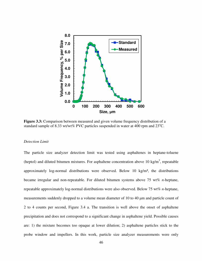
46
Figure 3.3: Comparison between measured and given volume frequency distribution of a
standard sample of 8.33 wt/wt% PVC particles suspended in water at 400 rpm and 23oC.
Detection Limit
The particle size analyzer detection limit was tested using asphaltenes in heptane-toluene
(heptol) and diluted bitumen mixtures. For asphaltene concentration above 10 kg/m3, repeatable
approximately log-normal distributions were observed. Below 10 kg/m³, the distributions
became irregular and non-repeatable. For diluted bitumen systems above 75 wt% n-heptane,
repeatable approximately log-normal distributions were also observed. Below 75 wt% n-heptane,
measurements suddenly dropped to a volume mean diameter of 10 to 40 µm and particle count of
2 to 4 counts per second, Figure 3.4 a. The transition is well above the onset of asphaltene
precipitation and does not correspond to a significant change in asphaltene yield. Possible causes
are: 1) the mixture becomes too opaque at lower dilution; 2) asphaltene particles stick to the
probe window and impellers. In this work, particle size analyzer measurements were only
0.0
1.0
2.0
3.0
4.0
5.0
6.0
7.0
8.0
0 100 200 300 400 500 600
Vo
lum
e F
req
ue
nc
y, %
pe
r S
ize
Size, µm
Standard
Measured
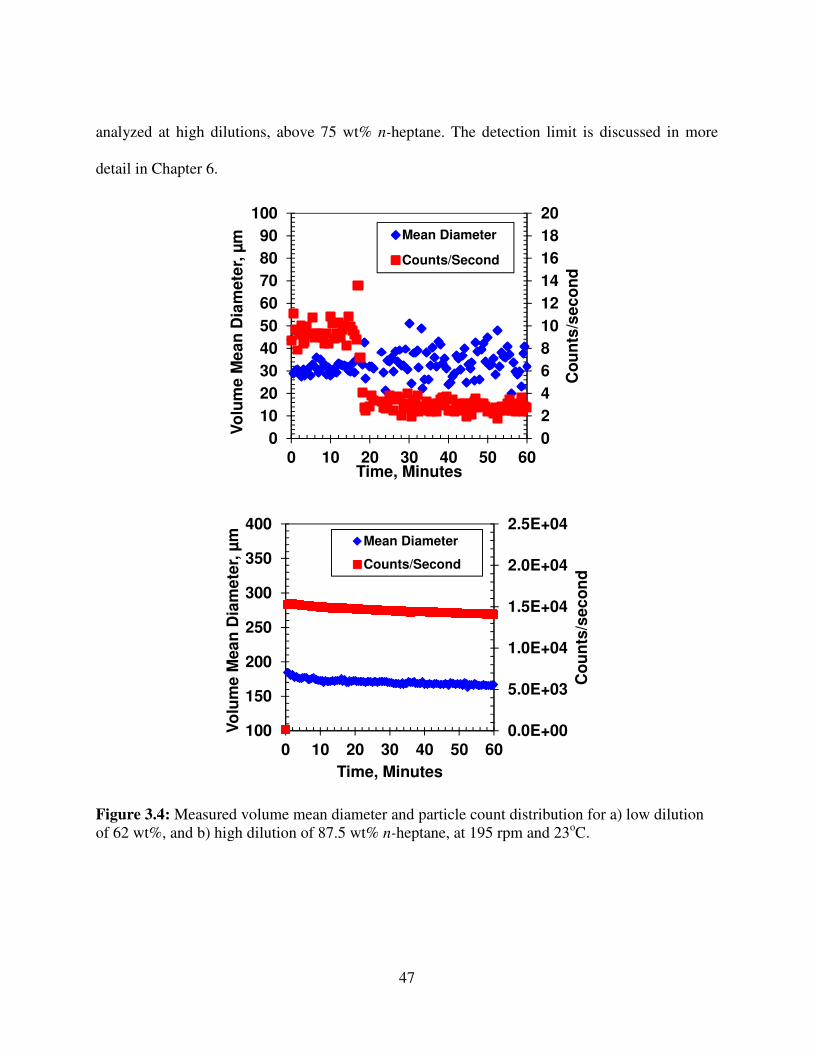
47
analyzed at high dilutions, above 75 wt% n-heptane. The detection limit is discussed in more
detail in Chapter 6.
Figure 3.4: Measured volume mean diameter and particle count distribution for a) low dilution
of 62 wt%, and b) high dilution of 87.5 wt% n-heptane, at 195 rpm and 23oC.
0
2
4
6
8
10
12
14
16
18
20
0
10
20
30
40
50
60
70
80
90
100
0 10 20 30 40 50 60
Co
un
ts/s
ec
on
d
Vo
lum
e M
ea
n D
iam
ete
r, µ
m
Time, Minutes
Mean Diameter
Counts/Second
0.0E+00
5.0E+03
1.0E+04
1.5E+04
2.0E+04
2.5E+04
100
150
200
250
300
350
400
0 10 20 30 40 50 60
Co
un
ts/s
ec
on
d
Vo
lum
e M
ea
n D
iam
ete
r, µ
m
Time, Minutes
Mean Diameter
Counts/Second
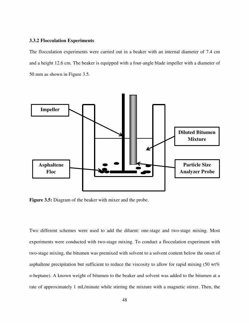
48
3.3.2 Flocculation Experiments
The flocculation experiments were carried out in a beaker with an internal diameter of 7.4 cm
and a height 12.6 cm. The beaker is equipped with a four-angle blade impeller with a diameter of
50 mm as shown in Figure 3.5.
Figure 3.5: Diagram of the beaker with mixer and the probe.
Two different schemes were used to add the diluent: one-stage and two-stage mixing. Most
experiments were conducted with two-stage mixing. To conduct a flocculation experiment with
two-stage mixing, the bitumen was premixed with solvent to a solvent content below the onset of
asphaltene precipitation but sufficient to reduce the viscosity to allow for rapid mixing (50 wt%
n-heptane). A known weight of bitumen to the beaker and solvent was added to the bitumen at a
rate of approximately 1 mL/minute while stirring the mixture with a magnetic stirrer. Then, the
Impeller
Asphaltene
Floc
Particle Size
Analyzer Probe
Diluted Bitumen
Mixture
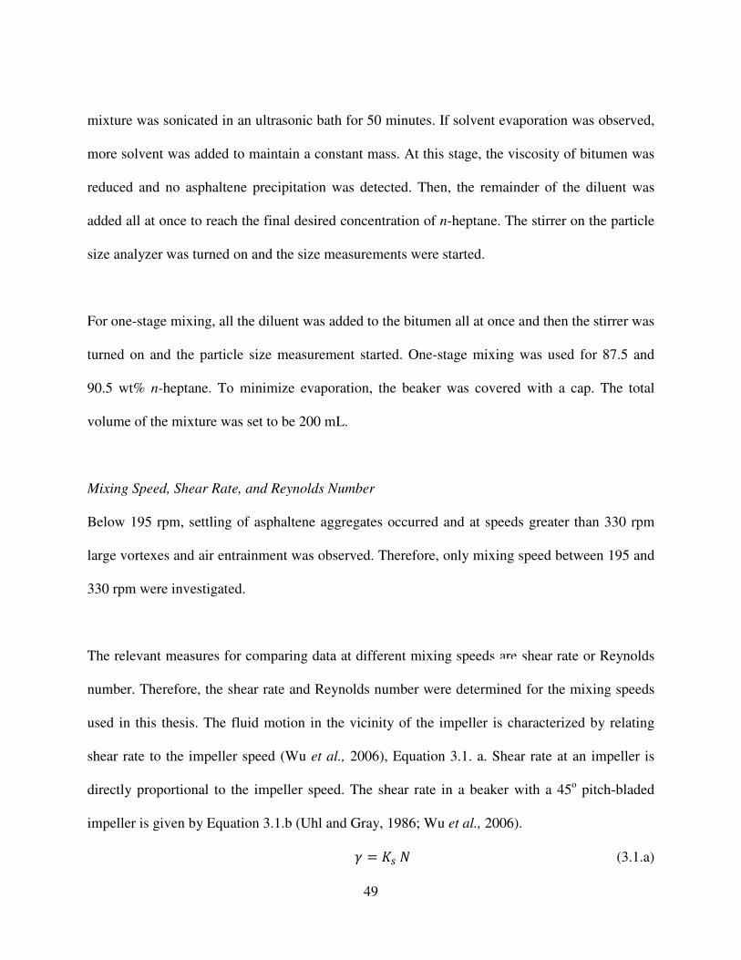
49
mixture was sonicated in an ultrasonic bath for 50 minutes. If solvent evaporation was observed,
more solvent was added to maintain a constant mass. At this stage, the viscosity of bitumen was
reduced and no asphaltene precipitation was detected. Then, the remainder of the diluent was
added all at once to reach the final desired concentration of n-heptane. The stirrer on the particle
size analyzer was turned on and the size measurements were started.
For one-stage mixing, all the diluent was added to the bitumen all at once and then the stirrer was
turned on and the particle size measurement started. One-stage mixing was used for 87.5 and
90.5 wt% n-heptane. To minimize evaporation, the beaker was covered with a cap. The total
volume of the mixture was set to be 200 mL.
Mixing Speed, Shear Rate, and Reynolds Number
Below 195 rpm, settling of asphaltene aggregates occurred and at speeds greater than 330 rpm
large vortexes and air entrainment was observed. Therefore, only mixing speed between 195 and
330 rpm were investigated.
The relevant measures for comparing data at different mixing speeds are shear rate or Reynolds
number. Therefore, the shear rate and Reynolds number were determined for the mixing speeds
used in this thesis. The fluid motion in the vicinity of the impeller is characterized by relating
shear rate to the impeller speed (Wu et al., 2006), Equation 3.1. a. Shear rate at an impeller is
directly proportional to the impeller speed. The shear rate in a beaker with a 45o pitch-bladed
impeller is given by Equation 3.1.b (Uhl and Gray, 1986; Wu et al., 2006).
6 = &78 (3.1.a)
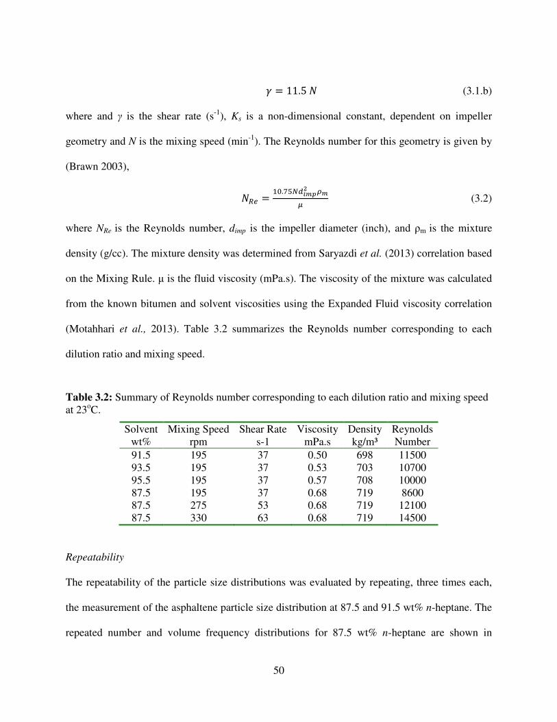
50
6 = 11.58 (3.1.b)
where and γ is the shear rate (s-1
), Ks is a non-dimensional constant, dependent on impeller
geometry and N is the mixing speed (min-1
). The Reynolds number for this geometry is given by
(Brawn 2003),
8;< = �=.>?@3ABCD EBF (3.2)
where NRe is the Reynolds number, dimp is the impeller diameter (inch), and ρm is the mixture
density (g/cc). The mixture density was determined from Saryazdi et al. (2013) correlation based
on the Mixing Rule. µ is the fluid viscosity (mPa.s). The viscosity of the mixture was calculated
from the known bitumen and solvent viscosities using the Expanded Fluid viscosity correlation
(Motahhari et al., 2013). Table 3.2 summarizes the Reynolds number corresponding to each
dilution ratio and mixing speed.
Table 3.2: Summary of Reynolds number corresponding to each dilution ratio and mixing speed
at 23oC.
Solvent
wt%
Mixing Speed
rpm
Shear Rate
s-1
Viscosity
mPa.s
Density
kg/m³
Reynolds
Number
91.5 195 37 0.50 698 11500
93.5 195 37 0.53 703 10700
95.5 195 37 0.57 708 10000
87.5 195 37 0.68 719 8600
87.5 275 53 0.68 719 12100
87.5 330 63 0.68 719 14500
Repeatability
The repeatability of the particle size distributions was evaluated by repeating, three times each,
the measurement of the asphaltene particle size distribution at 87.5 and 91.5 wt% n-heptane. The
repeated number and volume frequency distributions for 87.5 wt% n-heptane are shown in
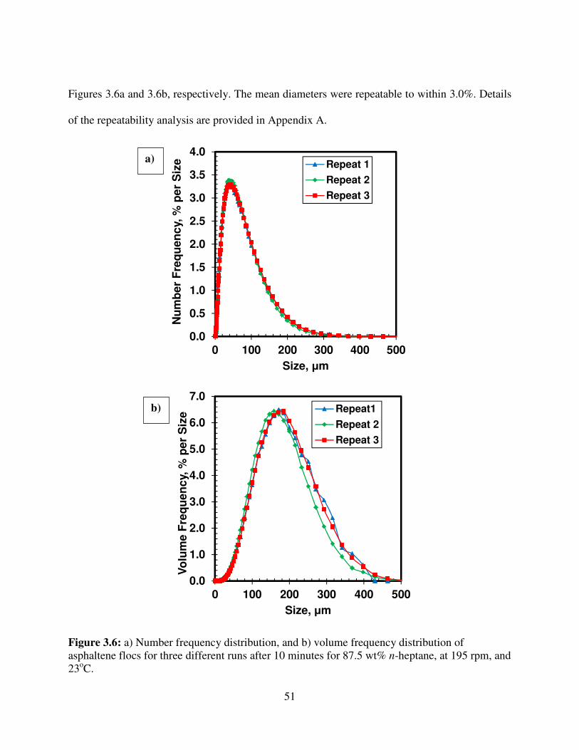
51
Figures 3.6a and 3.6b, respectively. The mean diameters were repeatable to within 3.0%. Details
of the repeatability analysis are provided in Appendix A.
Figure 3.6: a) Number frequency distribution, and b) volume frequency distribution of
asphaltene flocs for three different runs after 10 minutes for 87.5 wt% n-heptane, at 195 rpm, and
23oC.
0.0
0.5
1.0
1.5
2.0
2.5
3.0
3.5
4.0
0 100 200 300 400 500
Nu
mb
er
Fre
qu
en
cy,
% p
er
Siz
e
Size, µm
Repeat 1
Repeat 2
Repeat 3
0.0
1.0
2.0
3.0
4.0
5.0
6.0
7.0
0 100 200 300 400 500
Vo
lum
e F
req
ue
nc
y, %
pe
r S
ize
Size, µm
Repeat1
Repeat 2
Repeat 3
a)
b)
52
CHAPTER FOUR: : KINETICS OF ASPHALTENE PRECIPITATION
This chapter focuses on determining the onset and kinetics of asphaltene precipitation from a
Western Canadian bitumen diluted with n-heptane at 23oC, in both air and nitrogen atmospheres.
The data are used to assess the impact of oxidation on asphaltene yield and precipitation kinetics.
The steady state yield in nitrogen is then modeled using a regular solution approach. The effect
of the type of solvent on the kinetics of asphaltene precipitation is also investigated briefly.
4.1 Onset of Asphaltene Precipitation in n-Heptane Diluted Bitumen
The first step is to identify the onset of precipitation; that is, the solvent content at which
precipitation is first detectable as approximately 0.5 µm asphaltene particles. The onset of
precipitation was determined in two ways: by microscopic observation and gravimetrically. Both
methods were described in Chapter 3.
4.1.1 Onsets from Microscopic Method
Figure 4.1 shows the micrographs for the experimental runs with 56.5, 57, and 57.5 wt% n-
heptane at various times in an air atmosphere. The first appearance of particles is a haze that is
challenging to capture with a micrograph. This haze appears after 70, 40, and less than 1 minute
at 56.5, 57.0, and 57.5 wt%, n-heptane, respectively. After the haze is observed, clearly defined
particles and flocculation appear gradually over tens of minutes, Figures 4.1a to 4.1c,
respectively. Therefore, the appearance of the haze is interpreted as the onset of precipitation.
Figure 4.1 demonstrates that the onset of precipitation at time zero (immediately after mixing the
53
solvent in the bitumen) is 57.5 ± 0.5 wt% n-heptane. The onsets shift to lower n-heptane contents
with longer contact times, as summarized in Table 1. The shift to lower onsets and the gradual
growth in the number of particles over time confirm that asphaltene precipitation in air is time
dependent.
Table 4.1: Onset of asphaltene precipitation in n-heptane and n-pentane diluted WC_B2 bitumen
at 23°C and 1 atm.
Solvent Contact
Time (min)
Microscopic Onset
(wt% solvent)
Gravimetric Onset
(wt% solvent)
n-heptane < 1 57.5 ±0.5 -
n-heptane 40 57.0 ±0.5 -
n-heptane 70 56.5 ±0.5 -
n-heptane 120 - 56.5 ±1
n-pentane < 1 49.0 ±0.5 -
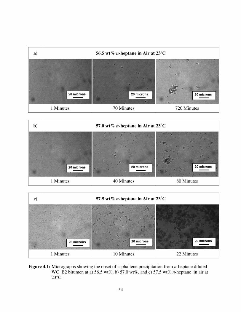
54
a) 56.5 wt% n-heptane in Air at 23oC
1 Minutes 70 Minutes 720 Minutes
b) 57.0 wt% n-heptane in Air at 23oC
1 Minutes 40 Minutes 80 Minutes
c) 57.5 wt% n-heptane in Air at 23oC
1 Minutes 10 Minutes 22 Minutes
Figure 4.1: Micrographs showing the onset of asphaltene precipitation from n-heptane diluted
WC_B2 bitumen at a) 56.5 wt%, b) 57.0 wt%, and c) 57.5 wt% n-heptane in air at
23°C.
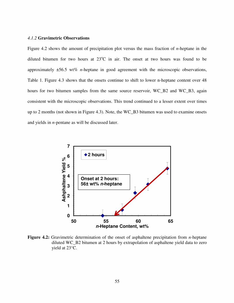
55
4.1.2 Gravimetric Observations
Figure 4.2 shows the amount of precipitation plot versus the mass fraction of n-heptane in the
diluted bitumen for two hours at 23oC in air. The onset at two hours was found to be
approximately ±56.5 wt% n-heptane in good agreement with the microscopic observations,
Table 1. Figure 4.3 shows that the onsets continue to shift to lower n-heptane content over 48
hours for two bitumen samples from the same source reservoir, WC_B2 and WC_B3, again
consistent with the microscopic observations. This trend continued to a lesser extent over times
up to 2 months (not shown in Figure 4.3). Note, the WC_B3 bitumen was used to examine onsets
and yields in n-pentane as will be discussed later.
Figure 4.2: Gravimetric determination of the onset of asphaltene precipitation from n-heptane
diluted WC_B2 bitumen at 2 hours by extrapolation of asphaltene yield data to zero
yield at 23°C.
0
1
2
3
4
5
6
7
50 55 60 65
Ash
ph
alt
en
e Y
ield
%
n-Heptane Content, wt%
2 hours
Onset at 2 hours:56± wt% n-heptane
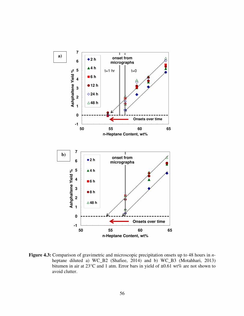
56
Figure 4.3: Comparison of gravimetric and microscopic precipitation onsets up to 48 hours in n-
heptane diluted a) WC_B2 (Shafiee, 2014) and b) WC_B3 (Motahhari, 2013)
bitumen in air at 23°C and 1 atm. Error bars in yield of ±0.61 wt% are not shown to
avoid clutter.
-1
0
1
2
3
4
5
6
7
50 55 60 65
As
hp
ha
lte
ne
Yie
ld %
n-Heptane Content, wt%
2 h
4 h
6 h
12 h
24 h
48 h
onset from micrographs
onset from micrographs
Onsets over time
-1
0
1
2
3
4
5
6
7
50 55 60 65
Ash
ph
alt
en
e Y
ield
%
n-Heptane Content, wt%
2 h
4 h
6 h
8 h
48 h
onset from micrographs
onset from micrographs
Onsets over time
a)
b)
t=0 t=1 hr
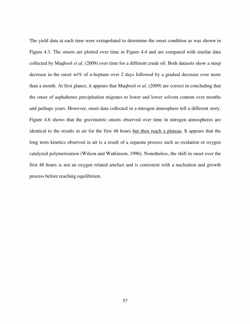
57
The yield data at each time were extrapolated to determine the onset condition as was shown in
Figure 4.3. The onsets are plotted over time in Figure 4.4 and are compared with similar data
collected by Maqbool et al. (2009) over time for a different crude oil. Both datasets show a steep
decrease in the onset wt% of n-heptane over 2 days followed by a gradual decrease over more
than a month. At first glance, it appears that Maqbool et al. (2009) are correct in concluding that
the onset of asphaltenes precipitation migrates to lower and lower solvent content over months
and perhaps years. However, onset data collected in a nitrogen atmosphere tell a different story.
Figure 4.6 shows that the gravimetric onsets observed over time in nitrogen atmospheres are
identical to the results in air for the first 48 hours but then reach a plateau. It appears that the
long term kinetics observed in air is a result of a separate process such as oxidation or oxygen
catalyzed polymerization (Wilson and Watkinson, 1996). Nonetheless, the shift in onset over the
first 48 hours is not an oxygen related artefact and is consistent with a nucleation and growth
process before reaching equilibrium.
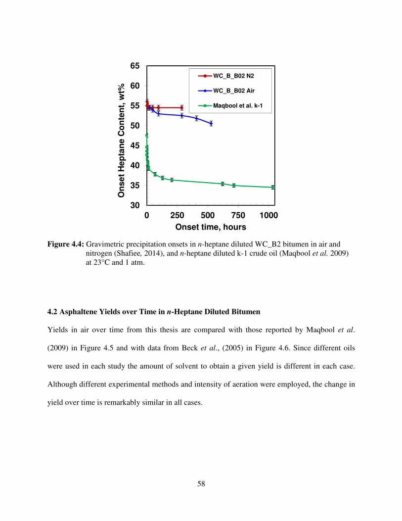
58
Figure 4.4: Gravimetric precipitation onsets in n-heptane diluted WC_B2 bitumen in air and
nitrogen (Shafiee, 2014), and n-heptane diluted k-1 crude oil (Maqbool et al. 2009)
at 23°C and 1 atm.
4.2 Asphaltene Yields over Time in n-Heptane Diluted Bitumen
Yields in air over time from this thesis are compared with those reported by Maqbool et al.
(2009) in Figure 4.5 and with data from Beck et al., (2005) in Figure 4.6. Since different oils
were used in each study the amount of solvent to obtain a given yield is different in each case.
Although different experimental methods and intensity of aeration were employed, the change in
yield over time is remarkably similar in all cases.
30
35
40
45
50
55
60
65
0 250 500 750 1000
On
se
t H
ep
tan
e C
on
ten
t, w
t%
Onset time, hours
WC_B_B02 N2
WC_B_B02 Air
Maqbool et al. k-1
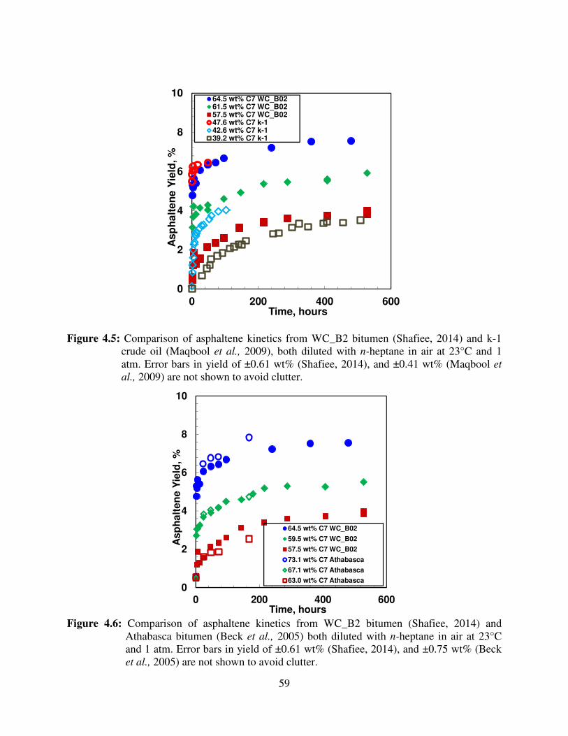
59
Figure 4.5: Comparison of asphaltene kinetics from WC_B2 bitumen (Shafiee, 2014) and k-1
crude oil (Maqbool et al., 2009), both diluted with n-heptane in air at 23°C and 1
atm. Error bars in yield of ±0.61 wt% (Shafiee, 2014), and ±0.41 wt% (Maqbool et
al., 2009) are not shown to avoid clutter.
Figure 4.6: Comparison of asphaltene kinetics from WC_B2 bitumen (Shafiee, 2014) and
Athabasca bitumen (Beck et al., 2005) both diluted with n-heptane in air at 23°C
and 1 atm. Error bars in yield of ±0.61 wt% (Shafiee, 2014), and ±0.75 wt% (Beck
et al., 2005) are not shown to avoid clutter.
0
2
4
6
8
10
0 200 400 600
Asp
ha
lte
ne
Yie
ld, %
Time, hours
64.5 wt% C7 WC_B0261.5 wt% C7 WC_B0257.5 wt% C7 WC_B0247.6 wt% C7 k-142.6 wt% C7 k-139.2 wt% C7 k-1
0
2
4
6
8
10
0 200 400 600
As
ph
alt
en
e Y
ield
, %
Time, hours
64.5 wt% C7 WC_B02
59.5 wt% C7 WC_B02
57.5 wt% C7 WC_B02
73.1 wt% C7 Athabasca
67.1 wt% C7 Athabasca
63.0 wt% C7 Athabasca
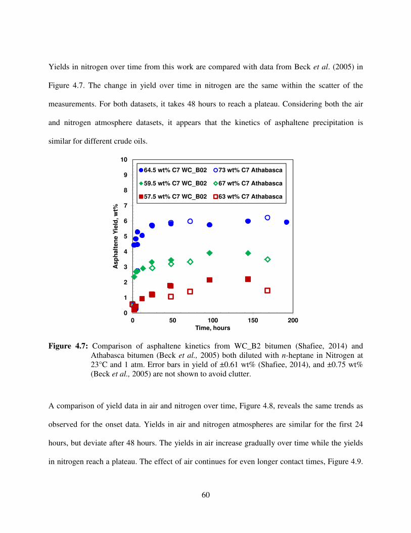
60
Yields in nitrogen over time from this work are compared with data from Beck et al. (2005) in
Figure 4.7. The change in yield over time in nitrogen are the same within the scatter of the
measurements. For both datasets, it takes 48 hours to reach a plateau. Considering both the air
and nitrogen atmosphere datasets, it appears that the kinetics of asphaltene precipitation is
similar for different crude oils.
Figure 4.7: Comparison of asphaltene kinetics from WC_B2 bitumen (Shafiee, 2014) and
Athabasca bitumen (Beck et al., 2005) both diluted with n-heptane in Nitrogen at
23°C and 1 atm. Error bars in yield of ±0.61 wt% (Shafiee, 2014), and ±0.75 wt%
(Beck et al., 2005) are not shown to avoid clutter.
A comparison of yield data in air and nitrogen over time, Figure 4.8, reveals the same trends as
observed for the onset data. Yields in air and nitrogen atmospheres are similar for the first 24
hours, but deviate after 48 hours. The yields in air increase gradually over time while the yields
in nitrogen reach a plateau. The effect of air continues for even longer contact times, Figure 4.9.
0
1
2
3
4
5
6
7
8
9
10
0 50 100 150 200
Asp
halt
en
e Y
ield
, w
t%
Time, hours
64.5 wt% C7 WC_B02 73 wt% C7 Athabasca
59.5 wt% C7 WC_B02 67 wt% C7 Athabasca
57.5 wt% C7 WC_B02 63 wt% C7 Athabasca
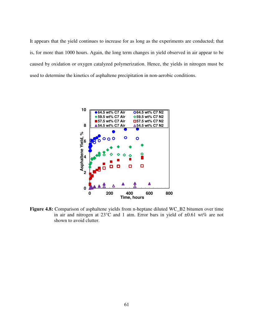
61
It appears that the yield continues to increase for as long as the experiments are conducted; that
is, for more than 1000 hours. Again, the long term changes in yield observed in air appear to be
caused by oxidation or oxygen catalyzed polymerization. Hence, the yields in nitrogen must be
used to determine the kinetics of asphaltene precipitation in non-aerobic conditions.
Figure 4.8: Comparison of asphaltene yields from n-heptane diluted WC_B2 bitumen over time
in air and nitrogen at 23°C and 1 atm. Error bars in yield of ±0.61 wt% are not
shown to avoid clutter.
0
2
4
6
8
10
0 200 400 600 800
As
ph
alt
en
e Y
ield
, %
Time, hours
64.5 wt% C7 Air 64.5 wt% C7 N2
59.5 wt% C7 Air 59.5 wt% C7 N257.5 wt% C7 Air 57.5 wt% C7 N2
54.5 wt% C7 Air 54.5 wt% C7 N2
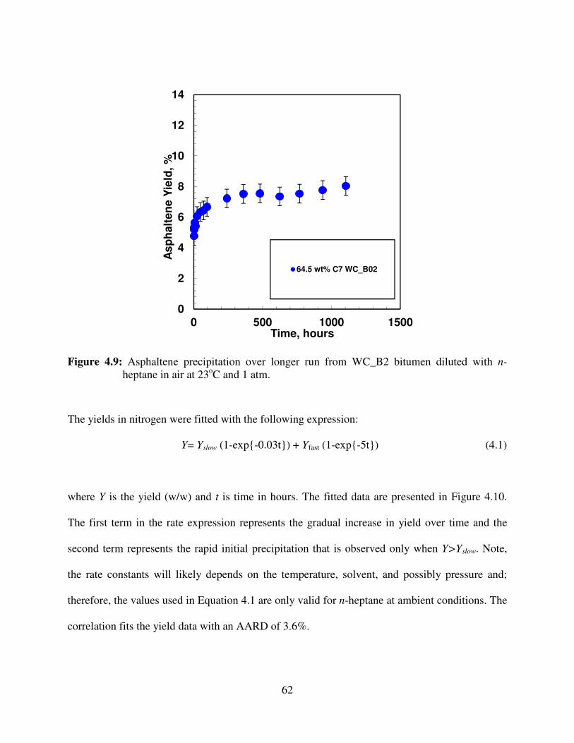
62
Figure 4.9: Asphaltene precipitation over longer run from WC_B2 bitumen diluted with n-
heptane in air at 23oC and 1 atm.
The yields in nitrogen were fitted with the following expression:
Y= Yslow (1-exp{-0.03t}) + Yfast (1-exp{-5t}) (4.1)
where Y is the yield (w/w) and t is time in hours. The fitted data are presented in Figure 4.10.
The first term in the rate expression represents the gradual increase in yield over time and the
second term represents the rapid initial precipitation that is observed only when Y>Yslow. Note,
the rate constants will likely depends on the temperature, solvent, and possibly pressure and;
therefore, the values used in Equation 4.1 are only valid for n-heptane at ambient conditions. The
correlation fits the yield data with an AARD of 3.6%.
0
2
4
6
8
10
12
14
0 500 1000 1500
As
ph
alt
en
e Y
ield
, %
Time, hours
64.5 wt% C7 WC_B02
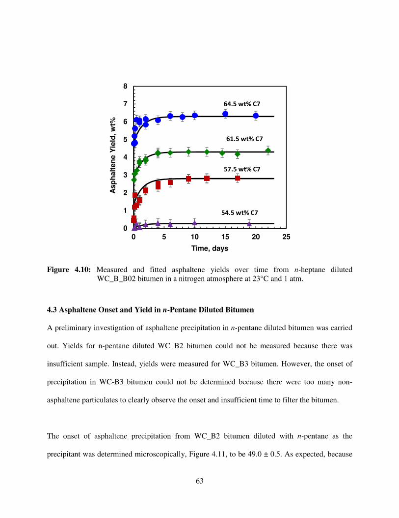
63
Figure 4.10: Measured and fitted asphaltene yields over time from n-heptane diluted
WC_B_B02 bitumen in a nitrogen atmosphere at 23°C and 1 atm.
4.3 Asphaltene Onset and Yield in n-Pentane Diluted Bitumen
A preliminary investigation of asphaltene precipitation in n-pentane diluted bitumen was carried
out. Yields for n-pentane diluted WC_B2 bitumen could not be measured because there was
insufficient sample. Instead, yields were measured for WC_B3 bitumen. However, the onset of
precipitation in WC-B3 bitumen could not be determined because there were too many non-
asphaltene particulates to clearly observe the onset and insufficient time to filter the bitumen.
The onset of asphaltene precipitation from WC_B2 bitumen diluted with n-pentane as the
precipitant was determined microscopically, Figure 4.11, to be 49.0 ± 0.5. As expected, because
0
1
2
3
4
5
6
7
8
0 5 10 15 20 25
Asp
halt
en
e Y
ield
, w
t%
Time, days
64.5 wt% C7
61.5 wt% C7
57.5 wt% C7
54.5 wt% C7
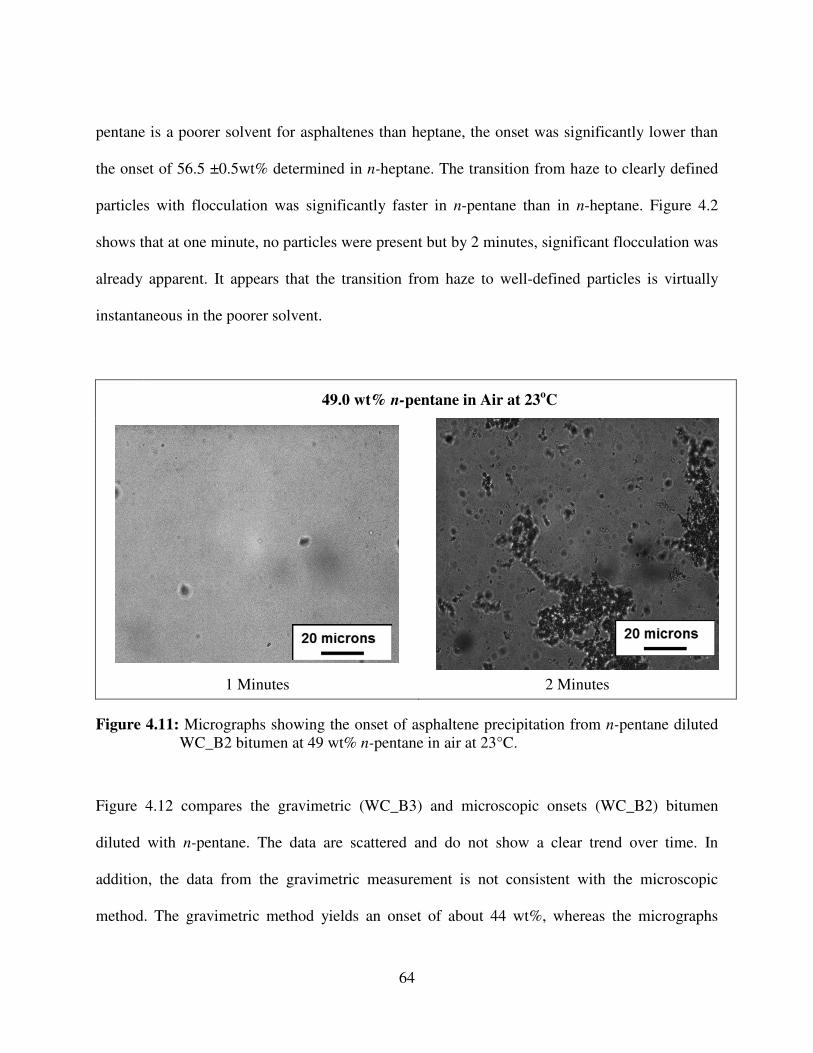
64
pentane is a poorer solvent for asphaltenes than heptane, the onset was significantly lower than
the onset of 56.5 ±0.5wt% determined in n-heptane. The transition from haze to clearly defined
particles with flocculation was significantly faster in n-pentane than in n-heptane. Figure 4.2
shows that at one minute, no particles were present but by 2 minutes, significant flocculation was
already apparent. It appears that the transition from haze to well-defined particles is virtually
instantaneous in the poorer solvent.
49.0 wt% n-pentane in Air at 23oC
1 Minutes 2 Minutes
Figure 4.11: Micrographs showing the onset of asphaltene precipitation from n-pentane diluted
WC_B2 bitumen at 49 wt% n-pentane in air at 23°C.
Figure 4.12 compares the gravimetric (WC_B3) and microscopic onsets (WC_B2) bitumen
diluted with n-pentane. The data are scattered and do not show a clear trend over time. In
addition, the data from the gravimetric measurement is not consistent with the microscopic
method. The gravimetric method yields an onset of about 44 wt%, whereas the micrographs
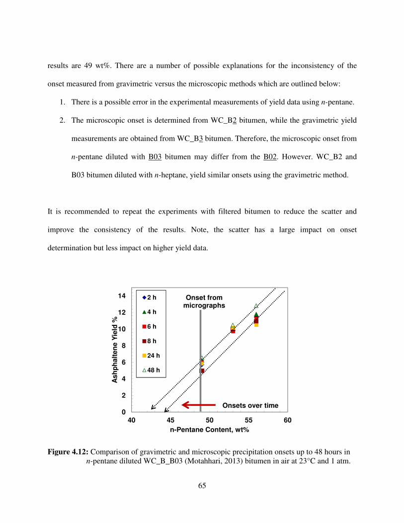
65
results are 49 wt%. There are a number of possible explanations for the inconsistency of the
onset measured from gravimetric versus the microscopic methods which are outlined below:
1. There is a possible error in the experimental measurements of yield data using n-pentane.
2. The microscopic onset is determined from WC_B2 bitumen, while the gravimetric yield
measurements are obtained from WC_B3 bitumen. Therefore, the microscopic onset from
n-pentane diluted with B03 bitumen may differ from the B02. However. WC_B2 and
B03 bitumen diluted with n-heptane, yield similar onsets using the gravimetric method.
It is recommended to repeat the experiments with filtered bitumen to reduce the scatter and
improve the consistency of the results. Note, the scatter has a large impact on onset
determination but less impact on higher yield data.
Figure 4.12: Comparison of gravimetric and microscopic precipitation onsets up to 48 hours in
n-pentane diluted WC_B_B03 (Motahhari, 2013) bitumen in air at 23°C and 1 atm.
0
2
4
6
8
10
12
14
40 45 50 55 60
As
hp
ha
lte
ne
Yie
ld %
n-Pentane Content, wt%
2 h
4 h
6 h
8 h
24 h
48 h
onset from micrographs
Onset from micrographs
Onsets over time
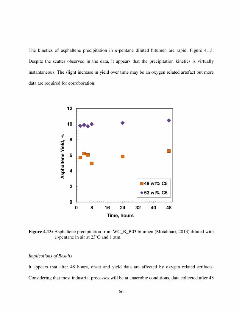
66
The kinetics of asphaltene precipitation in n-pentane diluted bitumen are rapid, Figure 4.13.
Despite the scatter observed in the data, it appears that the precipitation kinetics is virtually
instantaneous. The slight increase in yield over time may be an oxygen related artefact but more
data are required for corroboration.
Figure 4.13: Asphaltene precipitation from WC_B_B03 bitumen (Motahhari, 2013) diluted with
n-pentane in air at 23oC and 1 atm.
Implications of Results
It appears that after 48 hours, onset and yield data are affected by oxygen related artifacts.
Considering that most industrial processes will be at anaerobic conditions, data collected after 48
0
2
4
6
8
10
12
0 8 16 24 32 40 48
Asp
ha
lte
ne
Yie
ld, %
Time, hours
49 wt% C5
53 wt% C5
67
hours in air may not be valid. The “real” kinetic appears to take place within 48 hours. Therefore,
the relevant data can still be collected in air with negligible error.
One consequence of the observed kinetics is that the onsets determined within the first few hours
do not represent a thermodynamic equilibrium. In this work, the initial onset in n-heptane was
57.5 wt% while the apparent equilibrium onset is 54.5 wt%. Hence, some care is required in
choosing methods and data for particular asphaltene precipitation issues. For example, if the
target is data for a thermodynamic model, then data should be collected after approximately 24
hours. Short term titration data, such as those often collected with near-IR and visual
observations, will give misleading data for equilibrium models. On the other hand, if
precipitation at process conditions and residence times is of interest, short term titrations are the
appropriate choice. Equilibrium based models may give misleading results for short residence
time processes.
68
CHAPTER FIVE: ASPHALTENE FLOCCULATION MODEL
This chapter describes the Smoluchowski population balance equation used to model asphaltene
flocculation. First, the principles of the original model are shown and then the reaction terms
developed by Rastegari (2004) and Daneshvar (2005) for this model are discussed. Fractal
dimension is a key parameter in the model and in interpreting measured floc sizes and is
described in detail. Finally, the algorithm used to solve the population balance equations is
presented.
5.1 Smoluchowski Population Balance Equation for Asphaltene Flocculation Model
When particles in solution interact through molecular or colloidal forces and the convective
forces of a moving fluid, they will collide unless electrostatically stabilized. If flocculation is
reversible, collisions can result in flocculation, disintegration, or no net effect. Hence, the
number of flocs and number of particles in a floc is determined from the number of collisions
and the balance between the probabilities of flocculation and disintegration. The classical
Smoluchowski population balance, modified to include disintegration (Hamedi Rad et al., 2013;
Daneshvar, 2005; Rastegari et al., 2004; Rahmani et al., 2004), is used to model the reversible
flocculation and is given by:
( ) ( )∑ ∑=+
−
=
++++ −−−=kji
kN
j
jkjkjkjkjijijiji
k CDCCFCDCCFdt
dC
1
,,2
1 (5.1)
k=1,2,3,….,N
69
where the indices i, j, k, and N indicate the number of particles in the floc; Fi,j, and Di+j, are the
number of reactions (collisions) per unit volume per unit time that result in flocculation and
disintegration, respectively. Ci and Cj are the concentrations of species, while t is the time
(Rastegari et al., 2004). This model describes the rate of change of concentration of k-fold
aggregates, C k , under the assumption of binary collisions. These derivates are integrated over
finite time steps to update the calculated particle size distribution over time. The algorithm to
perform these calculations is presented later.
5.2 Flocculation and Disintegration Reaction Terms
The two characteristic time scales which govern flocculation kinetics are the diffusion time and
reaction time. Diffusion time (τdiff) is the time it takes for two arbitrary particles to approach to
the point of contact. Reaction time (τreac) is time it takes for two particles to flocculate when they
are in mutual proximity. The kinetics of flocculation is described as diffusion-limited in
instances where the diffusion time is greater than the reaction time. In this case, particles most
likely flocculate on their first encounter with a neighbor particle and the kinetics are influence by
local fluctuations in the concentration of the particles.
When the diffusion time is less than the reaction time, the kinetics is reaction-controlled and is
limited by the relatively large reaction time. In this case, a particle may sample large volumes of
its surrounding neighbors before flocculating and thus it effectively responds to the global
concentration of other particles. In other words, particles may come within reaction range of each
other numerous times before flocculation occurs. Reaction-limited flocculation is expected to be
70
the dominant mechanism in well-mixed experiments, like those used in this thesis, because
stirring homogenizes the local concentration.
5.2.1 Flocculation Reaction Term
Based on reaction-limited flocculation theory, the reaction terms are dependent on the
probability of bond formation upon collision of two clusters (Ball et al., 1987). Rastegari et al.
(2004) proposed the following reaction rate which is dependent on the reaction-limited
flocculation reaction theory:
λ
++
+′= ff D
j
ji
iD
i
ji
j
fji MMM
MM
MM
MkF
/1/1
, (5.2)
where k′f is the flocculation reaction constant scaled for mass, Mi is the mass of floc i, Df is the
fractal dimension of the floc, and λ is the flocculation reaction exponent which generally varies
between 2 and 3. The mass of a floc is directly proportional to the number of particles in the
floc; hence, Equation 5.2 can be expressed as follows (Daneshvar, 2005):
λ
++
+= ff D
j
ji
iD
i
ji
j
fji nnn
nn
nn
nkF
/1/1
, (5.3)
where kf is the flocculation reaction constant scaled for the number of particles and ni is the
number of particles in floc i, These equations ignore the effect of three-cluster flocculation and
were developed for low concentrations. Note that the flocculation reaction exponent decreases
with a higher fractal dimension (more compact flocs) because more compact flocs interpenetrate
less, which results in a less surface area of mutual contact (Rastegari, 2004).
71
5.2.2 Disintegration Reaction Term
The disintegration reaction term is expressed by a power law relationship to the particle diameter
and is given by (Rastegari et al., 2004; Daneshvar 2005):
( )ββ ff D
j
D
idjidji nnkRkD/1/1
+== ++ where jiji RRR +≈+ (5.4)
where i and j represent the two flocs formed when a larger floc of i+j breaks up, kd is the
disintegration reaction constant, Ri, Rj, are the radii of the flocs, and the disintegration reaction
exponent β is a number from 0 to 3. The assumption that Ri+j ≈ Ri + Rj is only valid when Ri >>
Rj or vice versa. For simplicity, Equation 5.4 has been used for all floc sizes. Note, the second
equality is obtained from the relationship between floc radius and fractal dimension which is
below.
5.3 Fractal Dimension
Aggregates that are clusters of monomers can have fractal structures, meaning that parts of the
objects are similar to the whole. This self-similar structure is characterized by fractal dimension
which is the measure of how the aggregates fill the space (Gmachowski, 2014; Kinsner, 2005).
Fractal dimension is a key parameter for the asphaltene flocculation model, not only because it
appears in the reaction terms, but also because it is used to scale the measured floc diameters to
the number of particles in the flocs.
Before introducing fractal dimension, first consider Euclidian dimensions. A mathematical
description of dimension is based on how the "size" of an object behaves as the linear dimension
increases. Consider a line segment as a one dimensional example. If the linear dimension of the
72
line segment is doubled, then based on the characteristic size, the length of the line has also
doubled. In two dimensional objects such as a rectangle, if the linear dimensions are doubled,
then the area increases by a factor of four. In three dimensional objects if the linear dimensions
are doubled then the volume increases by a factor of eight. The relationship between dimension
D, linear scaling R, and the resulting multiple increase in size or scaling factor, Sf, can be
generalized as follows:
GH = 4I (5.5)
Classical Euclidean geometry explains objects in integer dimensions. However, many things in
nature are described in non-integer dimensions, such as clouds, mountain ranges, and the stars in
the sky. For example, a straight line has a dimension of one, but a fractal curve, depending on
how much space it takes up as it curves and twists, has dimension between one and two. The
term fractal is used to describe objects that cannot be described using normal Euclidean
geometry. Fractals are characterized by a non-integer power law of dependence of the object
length and Equation 5.5 can be generalized as follows:
GH = 4IJ (5.6)
Mass or number scaling as a method for characterizing the structure of flocs containing fine
particles has received wide attention (Mullins and Sheu 1998). Figure 5.1 shows a floc of
individual particles that can be enclosed in a spherical volume of diameter, dm. The number of
particles (or mass) within the floc can be related to the diameter of the floc as follows:
KH ∝ 4IH (5.7)
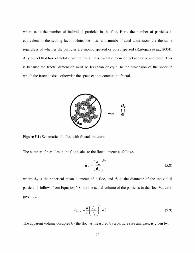
73
where nf is the number of individual particles in the floc. Here, the number of particles is
equivalent to the scaling factor. Note, the mass and number fractal dimensions are the same
regardless of whether the particles are monodispersed or polydispersed (Rastegari et al., 2004).
Any object that has a fractal structure has a mass fractal dimension between one and three. This
is because the fractal dimension must be less than or equal to the dimension of the space in
which the fractal exists, otherwise the space cannot contain the fractal.
Figure 5.1: Schematic of a floc with fractal structure.
The number of particles in the floc scales to the floc diameter as follows:
fD
p
m
fd
dn
= (5.8)
where dm is the spherical mean diameter of a floc, and dp is the diameter of the individual
particle. It follows from Equation 5.8 that the actual volume of the particles in the floc, Vactual, is
given by:
3
6p
D
p
m
actual dd
dV
f
=
π (5.9)
The apparent volume occupied by the floc, as measured by a particle size analyzer, is given by:
with
dp
dm
74
3
6mapp dV
π= (5.10)
Equations 5.9 and 5.10 will be used to interpret and model particle size distribution data for
flocculating asphaltenes.
An interesting consequence of fractal mass scaling is that the density of the fractal object
depends on its fractal dimension. The flocs become denser and more compact with increasing
fractal dimensions, as shown in Table 5.1. One consequence of this dimensional relationship is
that the fractal dimension can be estimated from the area projection of the floc. This is done by
analyzing the micrographs of the flocs. The two dimensional fractal dimension, Df2, can be
determined from the perimeter and the surface area of the flocs as follows:
2
2fD
PA = (5.11)
where A is surface area and P is perimeter
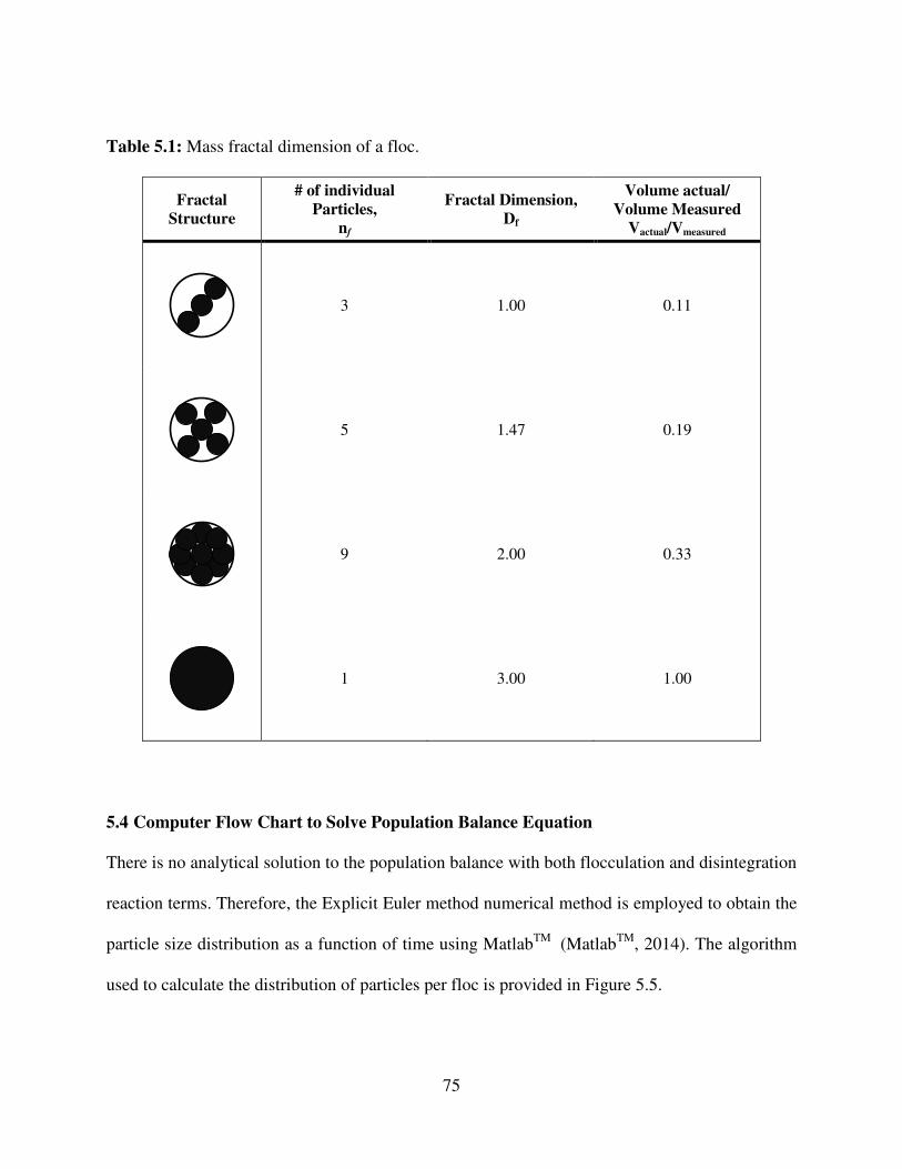
75
Table 5.1: Mass fractal dimension of a floc.
Fractal
Structure
# of individual
Particles,
nf
Fractal Dimension,
Df
Volume actual/
Volume Measured
Vactual/Vmeasured
3 1.00 0.11
5 1.47 0.19
9 2.00 0.33
1 3.00 1.00
5.4 Computer Flow Chart to Solve Population Balance Equation
There is no analytical solution to the population balance with both flocculation and disintegration
reaction terms. Therefore, the Explicit Euler method numerical method is employed to obtain the
particle size distribution as a function of time using MatlabTM
(MatlabTM
, 2014). The algorithm
used to calculate the distribution of particles per floc is provided in Figure 5.5.
76
The inputs to the model are the initial particle size distribution, the fractal dimension (Df), the
coefficients (kf and ks) and exponents (λ and β) for the two reaction terms, and the upper limit for
the number of particles per floc (N). The values of λ and β were set to the midpoint of their
permitted intervals, 2.5 and 1.5, and were not adjusted. The effect of adjusting λ and β is similar
to changing the kf/ks ratios. Hence, the model has three adjustable parameters, kf , ks, and Df. An
initial time step of 0.01 is also specified. The time step associated with Euler method is set to
ensure that total number of primary asphaltene particles remains constant during asphaltene
flocculation. The numerical error from too large a time step results in an error in total
concentration of individual particles.
In diluted bitumen systems, the largest floc could contain up to 1,200,000 individual particles at
a fractal dimension of 2.33, therefore the number of calculations required to perform a
population balance of individual particles becomes exhaustive for a practical numerical solution.
To reduce the computational time, the population balance is based on clusters of particles instead
of individual particles. A cluster of size 841 particles with mean diameter of 18 microns was
chosen to obtain simulation times less than 4 hours. The floc sizes ranged from 18 microns (1
cluster of 841 individual particles) to 396 microns (566 clusters and a total of 11,28,833
individual particles). In other words, the distribution of flocs was divided into 1344 bins so that
the ith
bin contains i clusters of 841xi individual particles. The equations used to find the bin
sizes, the number of bins, and the numbers of asphaltene primary particles of the bins are all
presented in Appendix B.
77
At each iteration, the reaction terms are calculated from Equations 5.3 and 5.4 and the change in
concentration of each floc size is determined from Equation 5.1. The concentrations are then
updated using Euler’s method:
][
][]1[
n
kn
k
n
kt
CCC
∆
∆+=
+ (5.12)
where superscript [n] indicates the nth
time step. Once the distribution is updated, a material
balance check is performed as follows:
]1[
1
][
1
−
==
−
= ∑∑
nN
k
k
nN
k
kerr kCkCMB (5.13)
where MBerr is the material balance error at each time step. If the material balance error exceeds
a 0.05 a smaller time step is selected and the iteration is repeated. When specified times are
reached, the concentration and apparent volume distribution of the flocs over time is printed.
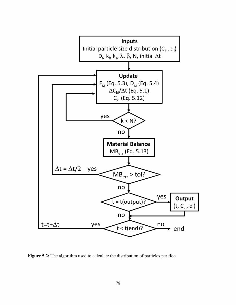
78
Figure 5.2: The algorithm used to calculate the distribution of particles per floc.
Inputs
Initial particle size distribution (Cki, di)
Df, kf, ks, λ, β, N, initial ∆t
Update
Fi,j (Eq. 5.3), Di,j (Eq. 5.4)
∆Cki/∆t (Eq. 5.1)
Cki (Eq. 5.12)
k < N?
Material Balance
MBerr (Eq. 5.13)
t = t(output)?
t < t(end)?
∆t = ∆t/2
yes
no
MBerr > tol?yes
no
Output
(t, Cki, di)
yest=t+∆tend
no
yes
no
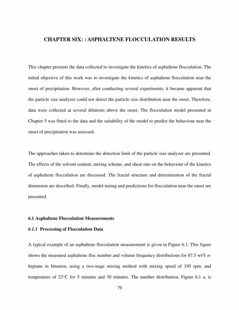
79
CHAPTER SIX: : ASPHALTENE FLOCCULATION RESULTS
This chapter presents the data collected to investigate the kinetics of asphaltene flocculation. The
initial objective of this work was to investigate the kinetics of asphaltene flocculation near the
onset of precipitation. However, after conducting several experiments, it became apparent that
the particle size analyzer could not detect the particle size distribution near the onset. Therefore,
data were collected at several dilutions above the onset. The flocculation model presented in
Chapter 5 was fitted to the data and the suitability of the model to predict the behaviour near the
onset of precipitation was assessed.
The approaches taken to determine the detection limit of the particle size analyzer are presented.
The effects of the solvent content, mixing scheme, and shear rate on the behaviour of the kinetics
of asphaltene flocculation are discussed. The fractal structure and determination of the fractal
dimension are described. Finally, model tuning and predictions for flocculation near the onset are
presented.
6.1 Asphaltene Flocculation Measurements
6.1.1 Processing of Flocculation Data
A typical example of an asphaltene flocculation measurement is given in Figure 6.1. This figure
shows the measured asphaltene floc number and volume frequency distributions for 87.5 wt% n-
heptane in bitumen, using a two-stage mixing method with mixing speed of 195 rpm, and
temperature of 23°C for 5 minutes and 30 minutes. The number distribution, Figure 6.1 a, is
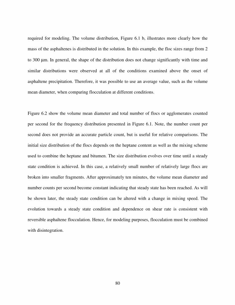
80
required for modeling. The volume distribution, Figure 6.1 b, illustrates more clearly how the
mass of the asphaltenes is distributed in the solution. In this example, the floc sizes range from 2
to 300 µm. In general, the shape of the distribution does not change significantly with time and
similar distributions were observed at all of the conditions examined above the onset of
asphaltene precipitation. Therefore, it was possible to use an average value, such as the volume
mean diameter, when comparing flocculation at different conditions.
Figure 6.2 show the volume mean diameter and total number of flocs or agglomerates counted
per second for the frequency distribution presented in Figure 6.1. Note, the number count per
second does not provide an accurate particle count, but is useful for relative comparisons. The
initial size distribution of the flocs depends on the heptane content as well as the mixing scheme
used to combine the heptane and bitumen. The size distribution evolves over time until a steady
state condition is achieved. In this case, a relatively small number of relatively large flocs are
broken into smaller fragments. After approximately ten minutes, the volume mean diameter and
number counts per second become constant indicating that steady state has been reached. As will
be shown later, the steady state condition can be altered with a change in mixing speed. The
evolution towards a steady state condition and dependence on shear rate is consistent with
reversible asphaltene flocculation. Hence, for modeling purposes, flocculation must be combined
with disintegration.
81
Figure 6.1: Measured asphaltene floc number (a) and volume frequency (b) distributions after 5
and 30 minutes for 87.5 wt% n-heptane diluted bitumen using two-stage mixing
method at 195 rpm and 23°C.
0.0
0.5
1.0
1.5
2.0
2.5
3.0
3.5
4.0
0 100 200 300 400 500
Nu
mb
er
Fre
qu
en
cy,
% p
er
Siz
e
Size, µm
5 Minutes
30 Minutes
0.0
1.0
2.0
3.0
4.0
5.0
6.0
7.0
0 100 200 300 400 500
Vo
lum
e F
req
ue
ncy,
% p
er
Siz
e
Size, µm
5 Minutes
30 Minutes
a)
b)
82
Figure 6.2: Volume mean diameter and number count of asphaltene flocculation over time from
87.5 wt% n-heptane diluted bitumen using the two-stage mixing method at a mixing
speed of 195 rpm, and 23°C.
6.1.2 Flocculation Data near the Onset of Asphaltene Precipitation
As discussed in Chapter 4, the onset of asphaltene precipitation from n-heptane diluted bitumen
was found to be 57.5 wt% n-heptane. Therefore, the particle size analyzer was first tested for a
series of diluted bitumen samples with n-heptane contents from 54.5 to 95.5 wt%. First, consider
the volume mean diameter and particle count for the samples at 61.5 and 65.0 wt% n-heptane,
Figure 6.3. In both cases, the particle count is very low, 2 to 4 counts per second in contrast with
a count of approximately 150,000 in the example shown in Figure 6.2. The volume mean
diameter is 10 to 40 µm and shows no pattern over time. The low particle count and scattered
mean diameter data suggest that noise has obscured any signal.
0.0E+00
5.0E+03
1.0E+04
1.5E+04
2.0E+04
2.5E+04
50
75
100
125
150
175
200
0 10 20 30
Co
un
ts/S
ec
on
d
Vo
lum
e M
ea
n D
iam
ete
r, µ
m
Time, Minutes
Mean Diameter
Counts/Second
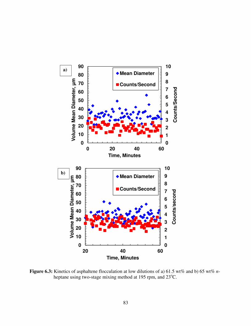
83
Figure 6.3: Kinetics of asphaltene flocculation at low dilutions of a) 61.5 wt% and b) 65 wt% n-
heptane using two-stage mixing method at 195 rpm, and 23oC.
0
1
2
3
4
5
6
7
8
9
10
0
10
20
30
40
50
60
70
80
90
0 20 40 60
Co
un
ts/S
ec
on
d
Vo
lum
e M
ea
n D
iam
ete
r, µ
m
Time, Minutes
Mean Diameter
Counts/Second
0
1
2
3
4
5
6
7
8
9
10
0
10
20
30
40
50
60
70
80
90
20 40 60
Co
un
ts/s
ec
on
d
Vo
lum
e M
ea
n D
iam
ete
r, µ
m
Time, Minutes
Mean Diameter
Counts/Second
a)
b)
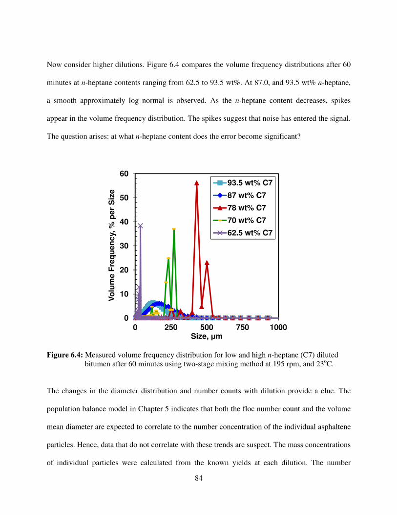
84
Now consider higher dilutions. Figure 6.4 compares the volume frequency distributions after 60
minutes at n-heptane contents ranging from 62.5 to 93.5 wt%. At 87.0, and 93.5 wt% n-heptane,
a smooth approximately log normal is observed. As the n-heptane content decreases, spikes
appear in the volume frequency distribution. The spikes suggest that noise has entered the signal.
The question arises: at what n-heptane content does the error become significant?
Figure 6.4: Measured volume frequency distribution for low and high n-heptane (C7) diluted
bitumen after 60 minutes using two-stage mixing method at 195 rpm, and 23oC.
The changes in the diameter distribution and number counts with dilution provide a clue. The
population balance model in Chapter 5 indicates that both the floc number count and the volume
mean diameter are expected to correlate to the number concentration of the individual asphaltene
particles. Hence, data that do not correlate with these trends are suspect. The mass concentrations
of individual particles were calculated from the known yields at each dilution. The number
0
10
20
30
40
50
60
0 250 500 750 1000
Vo
lum
e F
req
ue
nc
y, %
pe
r S
ize
Size, µm
93.5 wt% C7
87 wt% C7
78 wt% C7
70 wt% C7
62.5 wt% C7
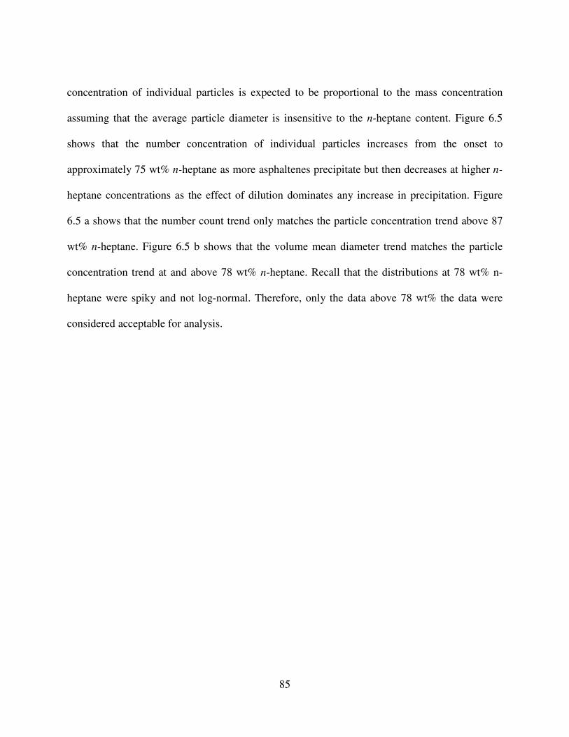
85
concentration of individual particles is expected to be proportional to the mass concentration
assuming that the average particle diameter is insensitive to the n-heptane content. Figure 6.5
shows that the number concentration of individual particles increases from the onset to
approximately 75 wt% n-heptane as more asphaltenes precipitate but then decreases at higher n-
heptane concentrations as the effect of dilution dominates any increase in precipitation. Figure
6.5 a shows that the number count trend only matches the particle concentration trend above 87
wt% n-heptane. Figure 6.5 b shows that the volume mean diameter trend matches the particle
concentration trend at and above 78 wt% n-heptane. Recall that the distributions at 78 wt% n-
heptane were spiky and not log-normal. Therefore, only the data above 78 wt% the data were
considered acceptable for analysis.
86
Figure 6.5: Comparison of measured number count (a) and measured volume mean diameter (b)
with concentration of precipitated asphaltenes based on the yield data for 24 hours
presented in Chapter 4 at 23oC.
Possible reasons for the loss of signal at low dilution are: a low particle concentration,
deposition, and sedimentation and opacity of the fluid. Since the mixtures were well stirred and
0
2000
4000
6000
8000
10000
12000
14000
16000
18000
20000
0
5
10
15
20
25
30
35
40
50 60 70 80 90 100
Me
as
ure
d N
um
be
r C
ou
nts
/Se
co
nd
s
Co
nc
en
tra
tio
n o
f P
rec
ipit
ate
d
As
ph
alt
en
Pa
ric
les
g/L
n-heptane Content, wt %
Cppt g/L
Counts/Second
0
100
200
300
400
500
0
5
10
15
20
25
30
50 60 70 80 90 100
Me
as
ure
d V
olu
me M
ea
n
Dia
me
ter,
µm
Co
nc
en
tra
tio
n o
f P
rec
ipit
ate
d
As
ph
alt
en
Pa
ric
les g
/L
n-heptane Content, wt %
Cppt g/L
Mean Diameter
a)
b)
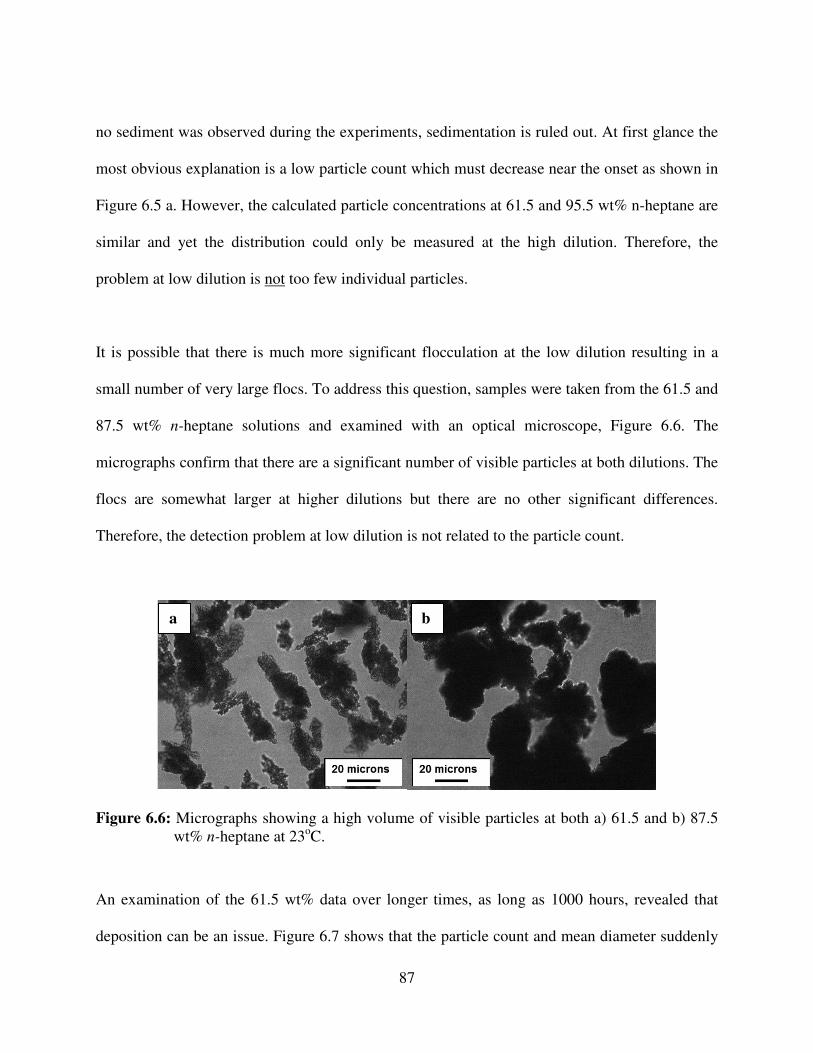
87
no sediment was observed during the experiments, sedimentation is ruled out. At first glance the
most obvious explanation is a low particle count which must decrease near the onset as shown in
Figure 6.5 a. However, the calculated particle concentrations at 61.5 and 95.5 wt% n-heptane are
similar and yet the distribution could only be measured at the high dilution. Therefore, the
problem at low dilution is not too few individual particles.
It is possible that there is much more significant flocculation at the low dilution resulting in a
small number of very large flocs. To address this question, samples were taken from the 61.5 and
87.5 wt% n-heptane solutions and examined with an optical microscope, Figure 6.6. The
micrographs confirm that there are a significant number of visible particles at both dilutions. The
flocs are somewhat larger at higher dilutions but there are no other significant differences.
Therefore, the detection problem at low dilution is not related to the particle count.
Figure 6.6: Micrographs showing a high volume of visible particles at both a) 61.5 and b) 87.5
wt% n-heptane at 23oC.
An examination of the 61.5 wt% data over longer times, as long as 1000 hours, revealed that
deposition can be an issue. Figure 6.7 shows that the particle count and mean diameter suddenly
a b
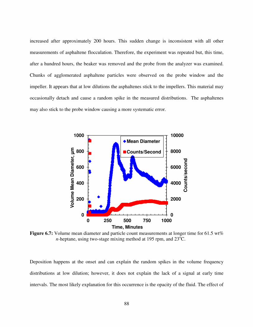
88
increased after approximately 200 hours. This sudden change is inconsistent with all other
measurements of asphaltene flocculation. Therefore, the experiment was repeated but, this time,
after a hundred hours, the beaker was removed and the probe from the analyzer was examined.
Chunks of agglomerated asphaltene particles were observed on the probe window and the
impeller. It appears that at low dilutions the asphaltenes stick to the impellers. This material may
occasionally detach and cause a random spike in the measured distributions. The asphaltenes
may also stick to the probe window causing a more systematic error.
Figure 6.7: Volume mean diameter and particle count measurements at longer time for 61.5 wt%
n-heptane, using two-stage mixing method at 195 rpm, and 23oC.
Deposition happens at the onset and can explain the random spikes in the volume frequency
distributions at low dilution; however, it does not explain the lack of a signal at early time
intervals. The most likely explanation for this occurrence is the opacity of the fluid. The effect of
0
2000
4000
6000
8000
10000
0
200
400
600
800
1000
0 250 500 750 1000
Co
un
ts/s
ec
on
d
Vo
lum
e M
ea
n D
iam
ete
r, µ
m
Time, Minutes
Mean Diameter
Counts/Second
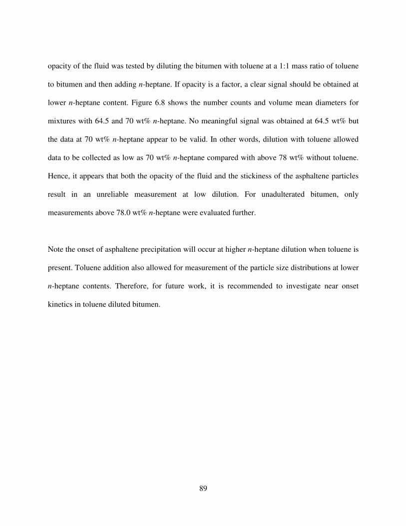
89
opacity of the fluid was tested by diluting the bitumen with toluene at a 1:1 mass ratio of toluene
to bitumen and then adding n-heptane. If opacity is a factor, a clear signal should be obtained at
lower n-heptane content. Figure 6.8 shows the number counts and volume mean diameters for
mixtures with 64.5 and 70 wt% n-heptane. No meaningful signal was obtained at 64.5 wt% but
the data at 70 wt% n-heptane appear to be valid. In other words, dilution with toluene allowed
data to be collected as low as 70 wt% n-heptane compared with above 78 wt% without toluene.
Hence, it appears that both the opacity of the fluid and the stickiness of the asphaltene particles
result in an unreliable measurement at low dilution. For unadulterated bitumen, only
measurements above 78.0 wt% n-heptane were evaluated further.
Note the onset of asphaltene precipitation will occur at higher n-heptane dilution when toluene is
present. Toluene addition also allowed for measurement of the particle size distributions at lower
n-heptane contents. Therefore, for future work, it is recommended to investigate near onset
kinetics in toluene diluted bitumen.
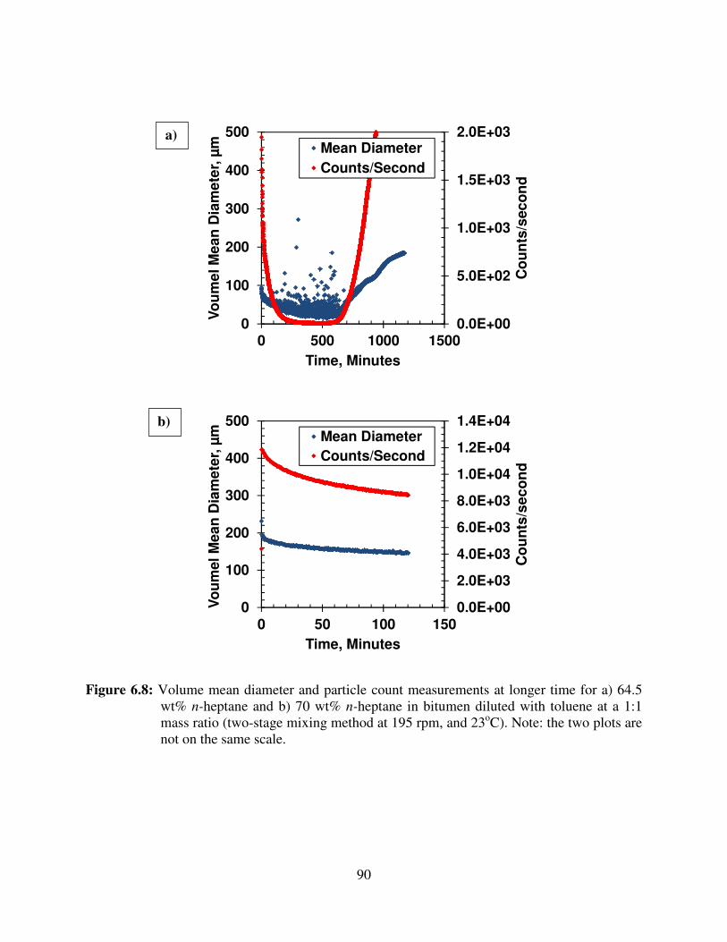
90
Figure 6.8: Volume mean diameter and particle count measurements at longer time for a) 64.5
wt% n-heptane and b) 70 wt% n-heptane in bitumen diluted with toluene at a 1:1
mass ratio (two-stage mixing method at 195 rpm, and 23oC). Note: the two plots are
not on the same scale.
0.0E+00
5.0E+02
1.0E+03
1.5E+03
2.0E+03
0
100
200
300
400
500
0 500 1000 1500
Co
un
ts/s
ec
on
d
Vo
um
el M
ea
n D
iam
ete
r, µ
m
Time, Minutes
Mean Diameter
Counts/Second
0.0E+00
2.0E+03
4.0E+03
6.0E+03
8.0E+03
1.0E+04
1.2E+04
1.4E+04
0
100
200
300
400
500
0 50 100 150
Co
un
ts/s
ec
on
d
Vo
um
el M
ea
n D
iam
ete
r, µ
m
Time, Minutes
Mean Diameter
Counts/Second
a)
b)
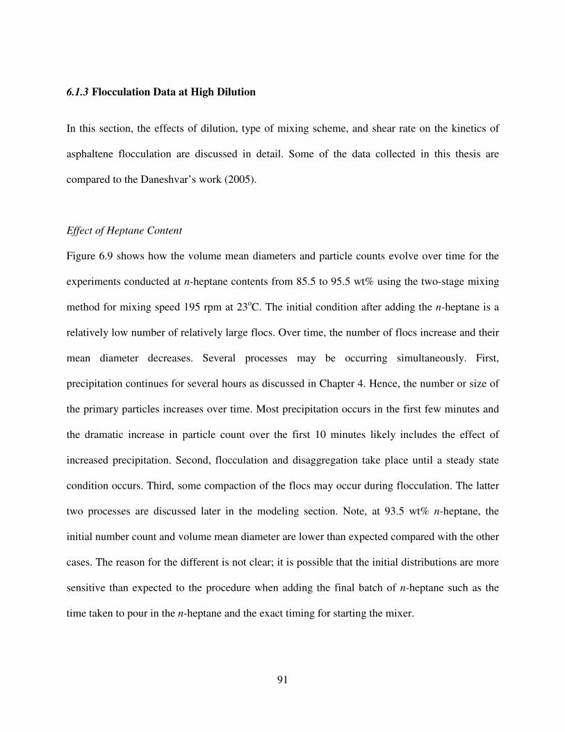
91
6.1.3 Flocculation Data at High Dilution
In this section, the effects of dilution, type of mixing scheme, and shear rate on the kinetics of
asphaltene flocculation are discussed in detail. Some of the data collected in this thesis are
compared to the Daneshvar’s work (2005).
Effect of Heptane Content
Figure 6.9 shows how the volume mean diameters and particle counts evolve over time for the
experiments conducted at n-heptane contents from 85.5 to 95.5 wt% using the two-stage mixing
method for mixing speed 195 rpm at 23oC. The initial condition after adding the n-heptane is a
relatively low number of relatively large flocs. Over time, the number of flocs increase and their
mean diameter decreases. Several processes may be occurring simultaneously. First,
precipitation continues for several hours as discussed in Chapter 4. Hence, the number or size of
the primary particles increases over time. Most precipitation occurs in the first few minutes and
the dramatic increase in particle count over the first 10 minutes likely includes the effect of
increased precipitation. Second, flocculation and disaggregation take place until a steady state
condition occurs. Third, some compaction of the flocs may occur during flocculation. The latter
two processes are discussed later in the modeling section. Note, at 93.5 wt% n-heptane, the
initial number count and volume mean diameter are lower than expected compared with the other
cases. The reason for the different is not clear; it is possible that the initial distributions are more
sensitive than expected to the procedure when adding the final batch of n-heptane such as the
time taken to pour in the n-heptane and the exact timing for starting the mixer.
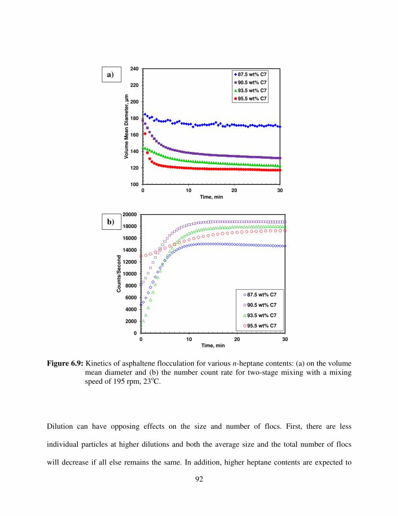
92
Figure 6.9: Kinetics of asphaltene flocculation for various n-heptane contents: (a) on the volume
mean diameter and (b) the number count rate for two-stage mixing with a mixing
speed of 195 rpm, 23oC.
Dilution can have opposing effects on the size and number of flocs. First, there are less
individual particles at higher dilutions and both the average size and the total number of flocs
will decrease if all else remains the same. In addition, higher heptane contents are expected to
100
120
140
160
180
200
220
240
0 10 20 30
Vo
lum
e M
ea
n D
iam
ete
r, µ
m
Time, min
87.5 wt% C7
90.5 wt% C7
93.5 wt% C7
95.5 wt% C7
0
2000
4000
6000
8000
10000
12000
14000
16000
18000
20000
0 10 20 30
Co
un
ts/S
eco
nd
Time, min
87.5 wt% C7
90.5 wt% C7
93.5 wt% C7
95.5 wt% C7
a)
b)
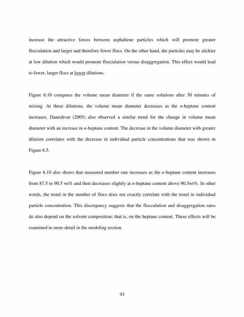
93
increase the attractive forces between asphaltene particles which will promote greater
flocculation and larger and therefore fewer flocs. On the other hand, the particles may be stickier
at low dilution which would promote flocculation versus disaggregation. This effect would lead
to fewer, larger flocs at lower dilutions.
Figure 6.10 compares the volume mean diameter if the same solutions after 30 minutes of
mixing. At these dilutions, the volume mean diameter decreases as the n-heptane content
increases. Daneshvar (2005) also observed a similar trend for the change in volume mean
diameter with an increase in n-heptane content. The decrease in the volume diameter with greater
dilution correlates with the decrease in individual particle concentrations that was shown in
Figure 6.5.
Figure 6.10 also shows that measured number rate increases as the n-heptane content increases
from 87.5 to 90.5 wt% and then decreases slightly at n-heptane content above 90.5wt%. In other
words, the trend in the number of flocs does not exactly correlate with the trend in individual
particle concentration. This discrepancy suggests that the flocculation and disaggregation rates
do also depend on the solvent composition; that is, on the heptane content. These effects will be
examined in more detail in the modeling section.
94
Figure 6.10: Effect of n-heptane content on the volume mean diameter and the number count
rate after 30 minutes in the two-stage mixing method at 195 rpm, and 23oC.
Effect of Mixing Scheme
As discussed in Chapter 3, two different mixing schemes were employed to induce asphaltene
flocculation. For one-stage mixing, all the diluent was added to the bitumen all at once and then
the stirrer was turned on and the particle size measurement started. One-stage mixing is more
representative of the industrial process. For two-stage mixing, the bitumen was premixed with
solvent to a solvent content below the onset of asphaltene precipitation, but sufficient to reduce
the viscosity to allow for rapid mixing (50 wt% n-heptane), and then the remainder of the diluent
was added all at once to reach the final desired concentration of n-heptane. Two-stage mixing
reduces the potential for artefacts related to poor mixing and therefore provides a better measure
of the “true” flocculation kinetics.
0
2000
4000
6000
8000
10000
12000
14000
16000
18000
20000
0
20
40
60
80
100
120
140
160
180
85 90 95 100
Co
un
ts/S
ec
on
d
Vo
lum
e M
ea
n D
iam
ete
r, µ
m
n-heptane Content, wt%
Mean Diameter
Counts/Second
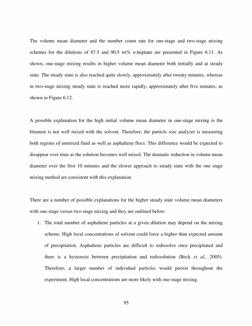
95
The volume mean diameter and the number count rate for one-stage and two-stage mixing
schemes for the dilutions of 87.5 and 90.5 wt% n-heptane are presented in Figure 6.11. As
shown, one-stage mixing results in higher volume mean diameter both initially and at steady
state. The steady state is also reached quite slowly, approximately after twenty minutes, whereas
in two-stage mixing steady state is reached more rapidly, approximately after five minutes, as
shown in Figure 6.12.
A possible explanation for the high initial volume mean diameter in one-stage mixing is the
bitumen is not well mixed with the solvent. Therefore, the particle size analyzer is measuring
both regions of unmixed fluid as well as asphaltene flocs. This difference would be expected to
disappear over time as the solution becomes well mixed. The dramatic reduction in volume mean
diameter over the first 10 minutes and the slower approach to steady state with the one stage
mixing method are consistent with this explanation.
There are a number of possible explanations for the higher steady state volume mean diameters
with one-stage versus two-stage mixing and they are outlined below:
1. The total number of asphaltene particles at a given dilution may depend on the mixing
scheme. High local concentrations of solvent could force a higher than expected amount
of precipitation. Asphaltene particles are difficult to redissolve once precipitated and
there is a hysteresis between precipitation and redissolution (Beck et al., 2005).
Therefore, a larger number of individual particles would persist throughout the
experiment. High local concentrations are more likely with one-stage mixing.
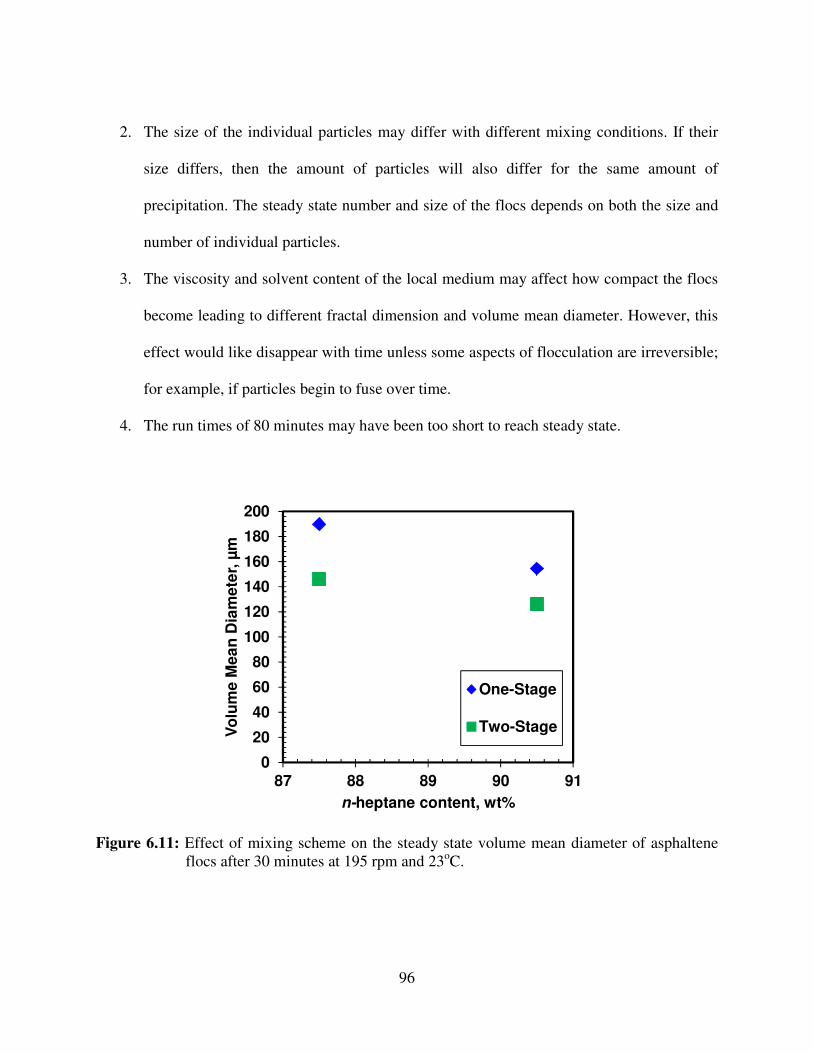
96
2. The size of the individual particles may differ with different mixing conditions. If their
size differs, then the amount of particles will also differ for the same amount of
precipitation. The steady state number and size of the flocs depends on both the size and
number of individual particles.
3. The viscosity and solvent content of the local medium may affect how compact the flocs
become leading to different fractal dimension and volume mean diameter. However, this
effect would like disappear with time unless some aspects of flocculation are irreversible;
for example, if particles begin to fuse over time.
4. The run times of 80 minutes may have been too short to reach steady state.
Figure 6.11: Effect of mixing scheme on the steady state volume mean diameter of asphaltene
flocs after 30 minutes at 195 rpm and 23oC.
0
20
40
60
80
100
120
140
160
180
200
87 88 89 90 91
Vo
lum
e M
ea
n D
iam
ete
r, µ
m
n-heptane content, wt%
One-Stage
Two-Stage
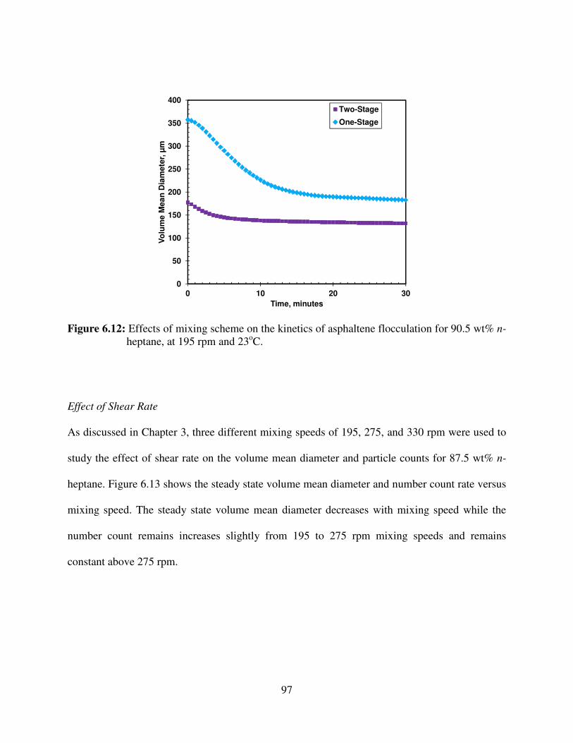
97
Figure 6.12: Effects of mixing scheme on the kinetics of asphaltene flocculation for 90.5 wt% n-
heptane, at 195 rpm and 23oC.
Effect of Shear Rate
As discussed in Chapter 3, three different mixing speeds of 195, 275, and 330 rpm were used to
study the effect of shear rate on the volume mean diameter and particle counts for 87.5 wt% n-
heptane. Figure 6.13 shows the steady state volume mean diameter and number count rate versus
mixing speed. The steady state volume mean diameter decreases with mixing speed while the
number count remains increases slightly from 195 to 275 rpm mixing speeds and remains
constant above 275 rpm.
0
50
100
150
200
250
300
350
400
0 10 20 30
Vo
lum
e M
ea
n D
iam
ete
r, µ
m
Time, minutes
Two-Stage
One-Stage
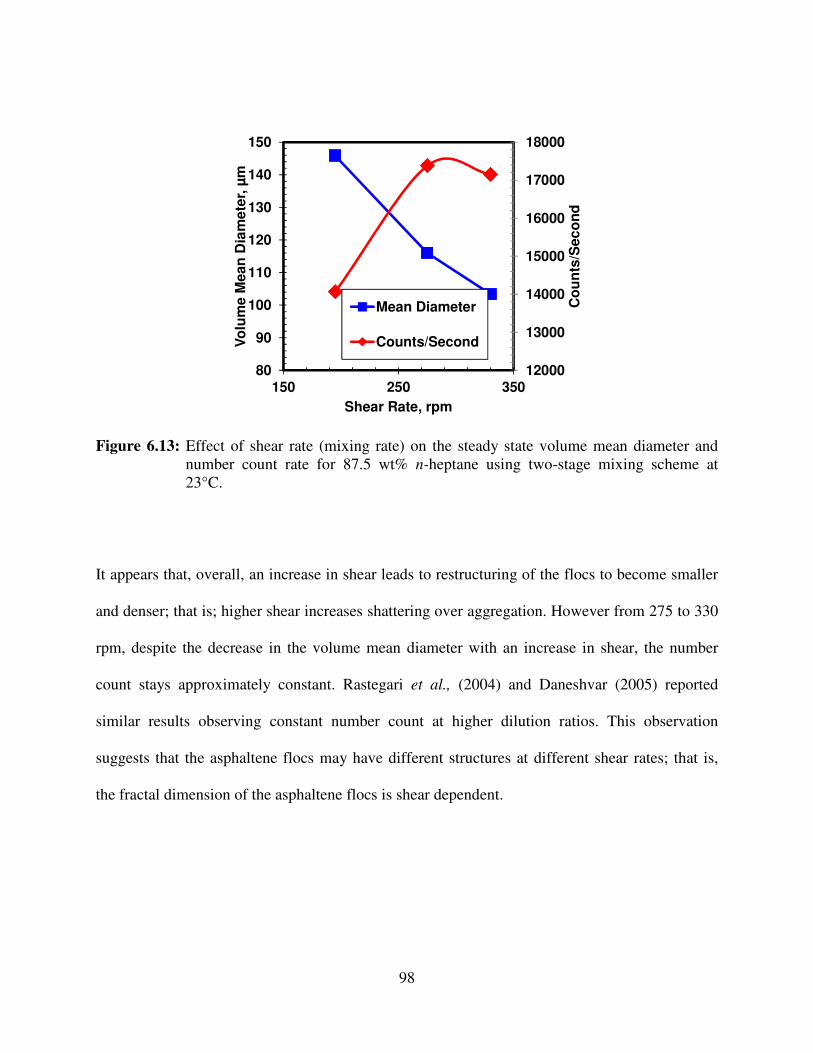
98
Figure 6.13: Effect of shear rate (mixing rate) on the steady state volume mean diameter and
number count rate for 87.5 wt% n-heptane using two-stage mixing scheme at
23°C.
It appears that, overall, an increase in shear leads to restructuring of the flocs to become smaller
and denser; that is; higher shear increases shattering over aggregation. However from 275 to 330
rpm, despite the decrease in the volume mean diameter with an increase in shear, the number
count stays approximately constant. Rastegari et al., (2004) and Daneshvar (2005) reported
similar results observing constant number count at higher dilution ratios. This observation
suggests that the asphaltene flocs may have different structures at different shear rates; that is,
the fractal dimension of the asphaltene flocs is shear dependent.
12000
13000
14000
15000
16000
17000
18000
80
90
100
110
120
130
140
150
150 250 350
Co
un
ts/S
ec
on
d
Vo
lum
e M
ean
Dia
me
ter,
µm
Shear Rate, rpm
Mean Diameter
Counts/Second
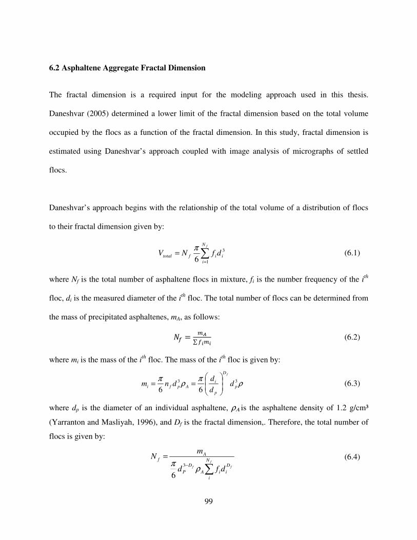
99
6.2 Asphaltene Aggregate Fractal Dimension
The fractal dimension is a required input for the modeling approach used in this thesis.
Daneshvar (2005) determined a lower limit of the fractal dimension based on the total volume
occupied by the flocs as a function of the fractal dimension. In this study, fractal dimension is
estimated using Daneshvar’s approach coupled with image analysis of micrographs of settled
flocs.
Daneshvar’s approach begins with the relationship of the total volume of a distribution of flocs
to their fractal dimension given by:
(6.1)
where Nf is the total number of asphaltene flocs in mixture, fi is the number frequency of the ith
floc, di is the measured diameter of the ith
floc. The total number of flocs can be determined from
the mass of precipitated asphaltenes, mA, as follows:
8H = MN∑HAMA (6.2)
where mi is the mass of the ith
floc. The mass of the ith
floc is given by:
(6.3)
where dp is the diameter of an individual asphaltene, ρΑ is the asphaltene density of 1.2 g/cm³
(Yarranton and Masliyah, 1996), and Df is the fractal dimension,. Therefore, the total number of
flocs is given by:
(6.4)
∑=
=fN
i
iiftotal dfNV1
3
6
π
ρπ
ρπ 33
66p
D
p
iApfi d
d
ddnm
f
==
∑−
=f
ff
N
i
D
iiA
D
P
Af
dfd
mN
ρπ 3
6
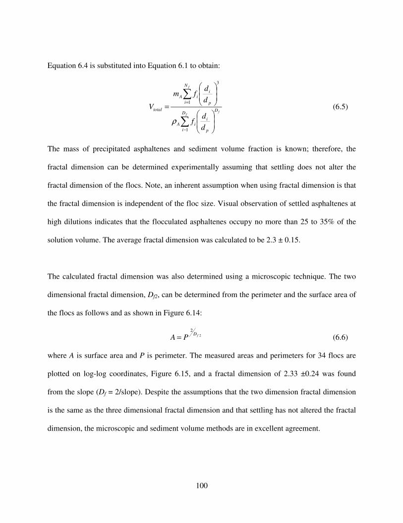
100
Equation 6.4 is substituted into Equation 6.1 to obtain:
(6.5)
The mass of precipitated asphaltenes and sediment volume fraction is known; therefore, the
fractal dimension can be determined experimentally assuming that settling does not alter the
fractal dimension of the flocs. Note, an inherent assumption when using fractal dimension is that
the fractal dimension is independent of the floc size. Visual observation of settled asphaltenes at
high dilutions indicates that the flocculated asphaltenes occupy no more than 25 to 35% of the
solution volume. The average fractal dimension was calculated to be 2.3 ± 0.15.
The calculated fractal dimension was also determined using a microscopic technique. The two
dimensional fractal dimension, Df2, can be determined from the perimeter and the surface area of
the flocs as follows and as shown in Figure 6.14:
(6.6)
where A is surface area and P is perimeter. The measured areas and perimeters for 34 flocs are
plotted on log-log coordinates, Figure 6.15, and a fractal dimension of 2.33 ±0.24 was found
from the slope (Df = 2/slope). Despite the assumptions that the two dimension fractal dimension
is the same as the three dimensional fractal dimension and that settling has not altered the fractal
dimension, the microscopic and sediment volume methods are in excellent agreement.
∑
∑
−
=
=f
f
f
D
i
D
p
iiA
N
i p
iiA
total
d
df
d
dfm
V
1
1
3
ρ
2
2fD
PA =
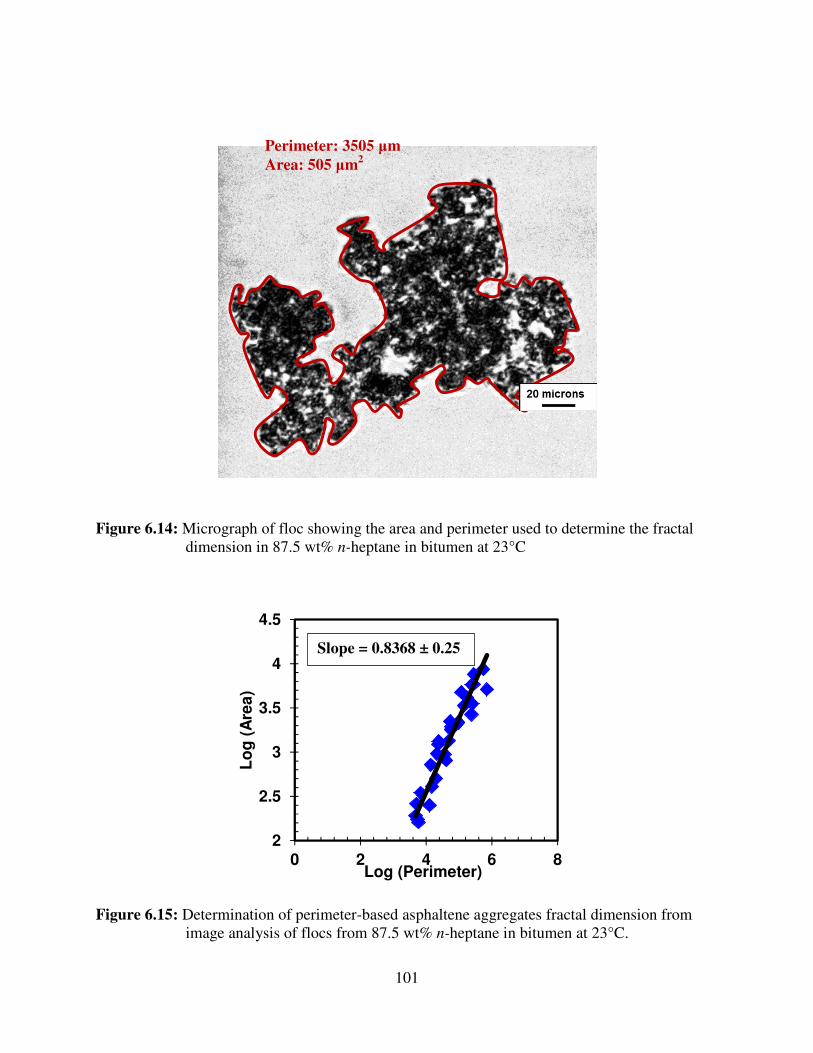
101
Figure 6.14: Micrograph of floc showing the area and perimeter used to determine the fractal
dimension in 87.5 wt% n-heptane in bitumen at 23°C
Figure 6.15: Determination of perimeter-based asphaltene aggregates fractal dimension from
image analysis of flocs from 87.5 wt% n-heptane in bitumen at 23°C.
2
2.5
3
3.5
4
4.5
0 2 4 6 8
Lo
g (
Are
a)
Log (Perimeter)
Perimeter: 3505 µm
Area: 505 µm2
Slope = 0.8368 ± 0.25
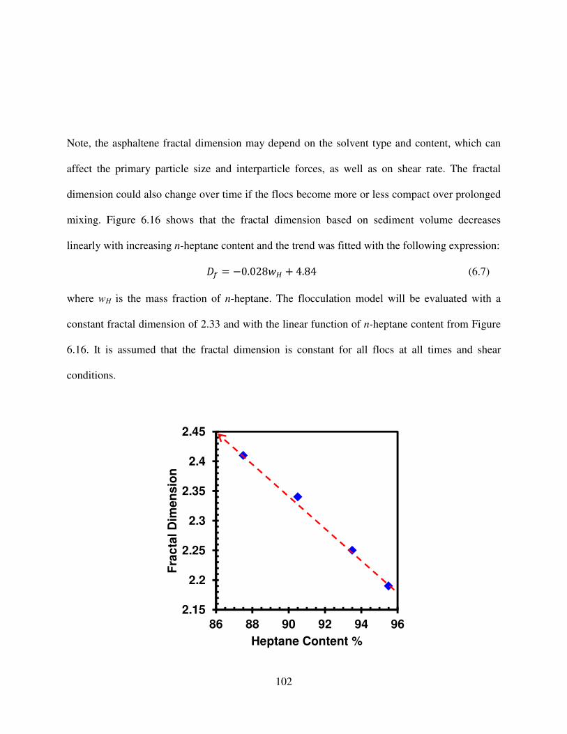
102
Note, the asphaltene fractal dimension may depend on the solvent type and content, which can
affect the primary particle size and interparticle forces, as well as on shear rate. The fractal
dimension could also change over time if the flocs become more or less compact over prolonged
mixing. Figure 6.16 shows that the fractal dimension based on sediment volume decreases
linearly with increasing n-heptane content and the trend was fitted with the following expression:
2H = −0.028QR + 4.84 (6.7)
where wH is the mass fraction of n-heptane. The flocculation model will be evaluated with a
constant fractal dimension of 2.33 and with the linear function of n-heptane content from Figure
6.16. It is assumed that the fractal dimension is constant for all flocs at all times and shear
conditions.
2.15
2.2
2.25
2.3
2.35
2.4
2.45
86 88 90 92 94 96
Fra
cta
l D
ime
ns
ion
Heptane Content %
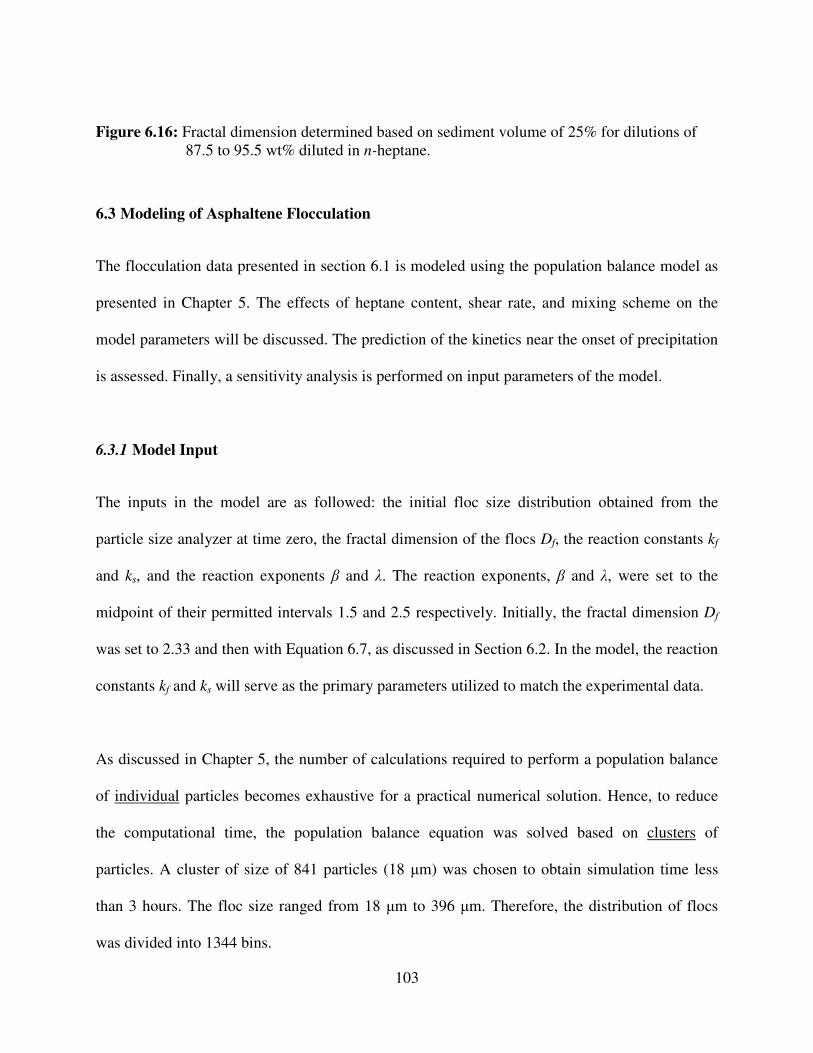
103
Figure 6.16: Fractal dimension determined based on sediment volume of 25% for dilutions of
87.5 to 95.5 wt% diluted in n-heptane.
6.3 Modeling of Asphaltene Flocculation
The flocculation data presented in section 6.1 is modeled using the population balance model as
presented in Chapter 5. The effects of heptane content, shear rate, and mixing scheme on the
model parameters will be discussed. The prediction of the kinetics near the onset of precipitation
is assessed. Finally, a sensitivity analysis is performed on input parameters of the model.
6.3.1 Model Input
The inputs in the model are as followed: the initial floc size distribution obtained from the
particle size analyzer at time zero, the fractal dimension of the flocs Df, the reaction constants kf
and ks, and the reaction exponents β and λ. The reaction exponents, β and λ, were set to the
midpoint of their permitted intervals 1.5 and 2.5 respectively. Initially, the fractal dimension Df
was set to 2.33 and then with Equation 6.7, as discussed in Section 6.2. In the model, the reaction
constants kf and ks will serve as the primary parameters utilized to match the experimental data.
As discussed in Chapter 5, the number of calculations required to perform a population balance
of individual particles becomes exhaustive for a practical numerical solution. Hence, to reduce
the computational time, the population balance equation was solved based on clusters of
particles. A cluster of size of 841 particles (18 µm) was chosen to obtain simulation time less
than 3 hours. The floc size ranged from 18 µm to 396 µm. Therefore, the distribution of flocs
was divided into 1344 bins.
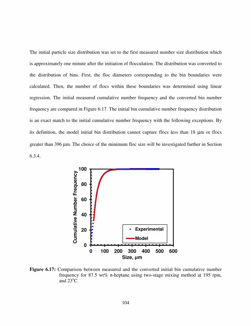
104
The initial particle size distribution was set to the first measured number size distribution which
is approximately one minute after the initiation of flocculation. The distribution was converted to
the distribution of bins. First, the floc diameters corresponding to the bin boundaries were
calculated. Then, the number of flocs within these boundaries was determined using linear
regression. The initial measured cumulative number frequency and the converted bin number
frequency are compared in Figure 6.17. The initial bin cumulative number frequency distribution
is an exact match to the initial cumulative number frequency with the following exceptions. By
its definition, the model initial bin distribution cannot capture flocs less than 18 µm or flocs
greater than 396 µm. The choice of the minimum floc size will be investigated further in Section
6.3.4.
Figure 6.17: Comparison between measured and the converted initial bin cumulative number
frequency for 87.5 wt% n-heptane using two-stage mixing method at 195 rpm,
and 23oC.
0
20
40
60
80
100
0 100 200 300 400 500 600
Cu
mu
lati
ve
Nu
mb
er
Fre
qu
en
cy
Size, µm
Experimental
Model
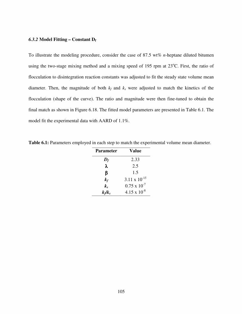
105
6.3.2 Model Fitting – Constant Df
To illustrate the modeling procedure, consider the case of 87.5 wt% n-heptane diluted bitumen
using the two-stage mixing method and a mixing speed of 195 rpm at 23oC. First, the ratio of
flocculation to disintegration reaction constants was adjusted to fit the steady state volume mean
diameter. Then, the magnitude of both kf and ks were adjusted to match the kinetics of the
flocculation (shape of the curve). The ratio and magnitude were then fine-tuned to obtain the
final match as shown in Figure 6.18. The fitted model parameters are presented in Table 6.1. The
model fit the experimental data with AARD of 1.1%.
Table 6.1: Parameters employed in each step to match the experimental volume mean diameter.
Parameter Value
Df 2.33
λλλλ 2.5
ββββ 1.5
kf 3.11 x 10⁻¹⁵
ks 0.75 x 10⁻⁷
kf/ks 4.15 x 10
-8
106
Figure 6.18: The fitted and experimental volume mean diameter for 87.5 wt% n-heptane using
two-stage mixing method at 195 rpm, and 23oC.
The model is able to capture the dynamics of volume mean diameter with time. However, at time
zero, the model volume mean diameter doesn’t quite match the experimental volume mean
diameter. It was found that the volume mean diameter is sensitive to truncation of the particle
number counts. After measurements, the experimental data are exported from the particle size
analyzer software to excel. It appears that during this process the number frequency distribution
is truncated by the software therefore the volume mean diameter used in the model are slightly
lower than used in the software.
The results of the model and the experimental cumulative volume frequency distribution for the
base case after 10 and 30 minutes are shown in Figure 6.19. The size intervals in the measured
and predicted distributions are not the same; therefore, the cumulative size distributions are
compared. It appears that the model underestimates the proportion of small flocs; this deviation
125
150
175
200
225
0 10 20 30 40 50
Vo
lum
e M
ea
n D
iam
ete
r, µ
m
Time, Minute
Experimental
Model
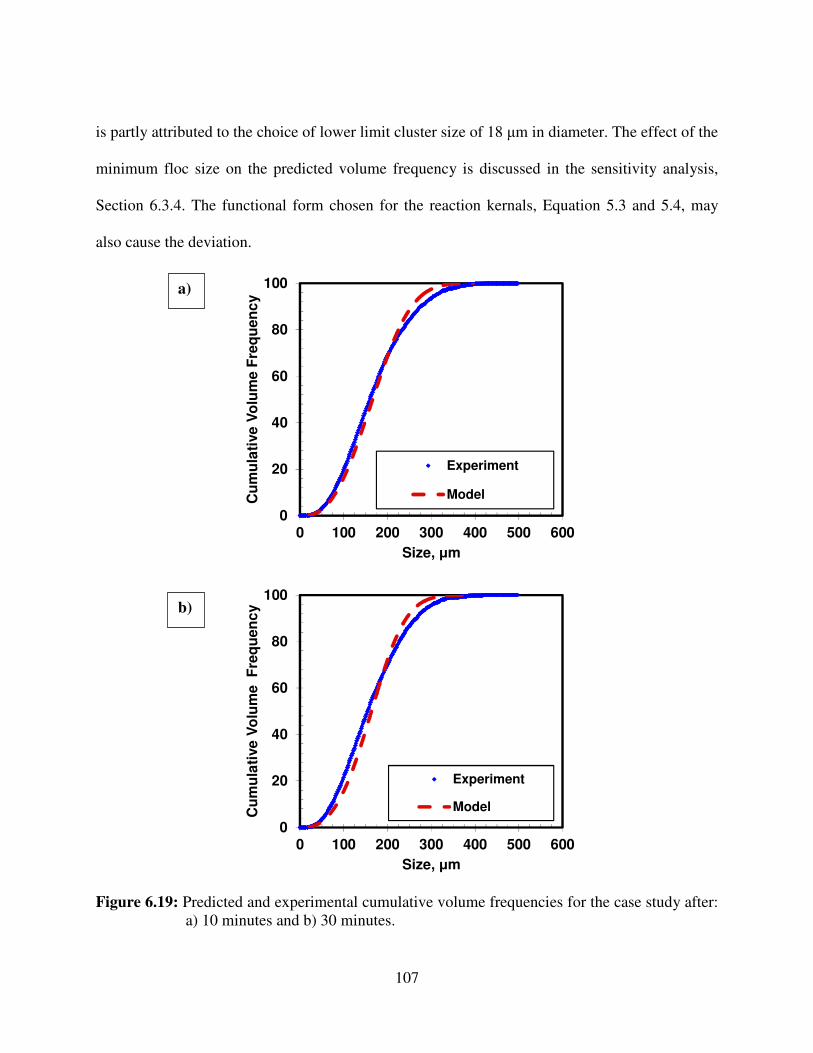
107
is partly attributed to the choice of lower limit cluster size of 18 µm in diameter. The effect of the
minimum floc size on the predicted volume frequency is discussed in the sensitivity analysis,
Section 6.3.4. The functional form chosen for the reaction kernals, Equation 5.3 and 5.4, may
also cause the deviation.
Figure 6.19: Predicted and experimental cumulative volume frequencies for the case study after:
a) 10 minutes and b) 30 minutes.
0
20
40
60
80
100
0 100 200 300 400 500 600
Cu
mu
lati
ve
Vo
lum
e F
req
uen
cy
Size, µm
Experiment
Model
0
20
40
60
80
100
0 100 200 300 400 500 600
Cu
mu
lati
ve
Vo
lum
e F
req
uen
cy
Size, µm
Experiment
Model
a)
b)
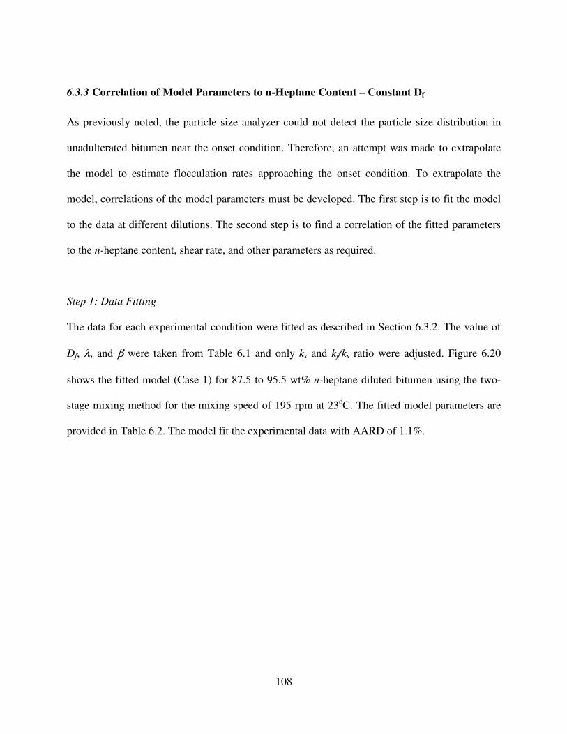
108
6.3.3 Correlation of Model Parameters to n-Heptane Content – Constant Df
As previously noted, the particle size analyzer could not detect the particle size distribution in
unadulterated bitumen near the onset condition. Therefore, an attempt was made to extrapolate
the model to estimate flocculation rates approaching the onset condition. To extrapolate the
model, correlations of the model parameters must be developed. The first step is to fit the model
to the data at different dilutions. The second step is to find a correlation of the fitted parameters
to the n-heptane content, shear rate, and other parameters as required.
Step 1: Data Fitting
The data for each experimental condition were fitted as described in Section 6.3.2. The value of
Df, λ, and β were taken from Table 6.1 and only ks and kf/ks ratio were adjusted. Figure 6.20
shows the fitted model (Case 1) for 87.5 to 95.5 wt% n-heptane diluted bitumen using the two-
stage mixing method for the mixing speed of 195 rpm at 23oC. The fitted model parameters are
provided in Table 6.2. The model fit the experimental data with AARD of 1.1%.
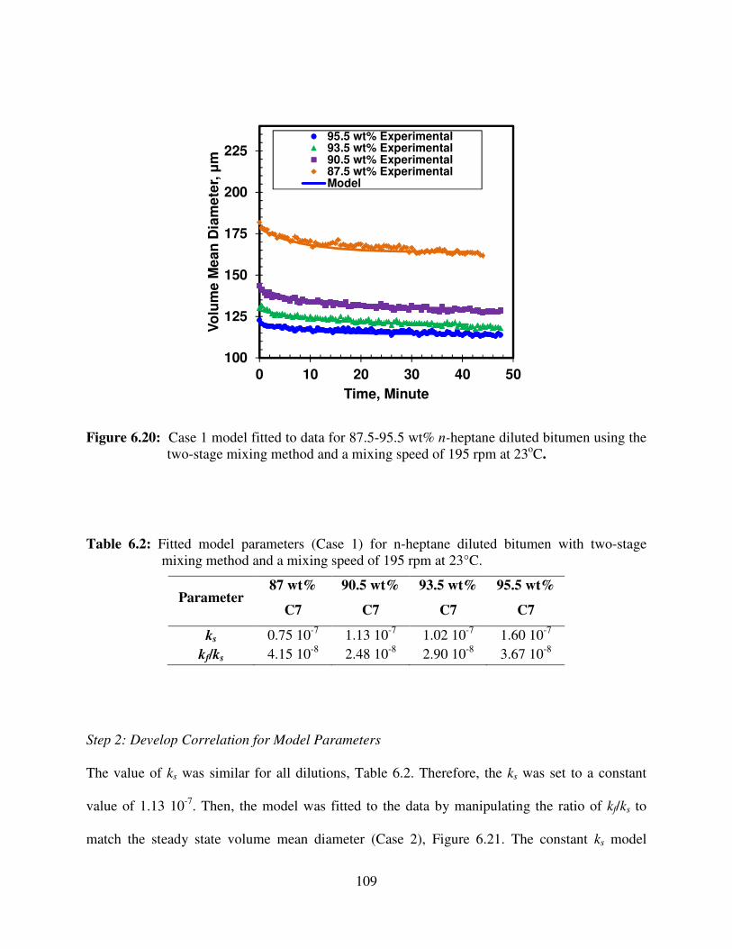
109
Figure 6.20: Case 1 model fitted to data for 87.5-95.5 wt% n-heptane diluted bitumen using the
two-stage mixing method and a mixing speed of 195 rpm at 23oC.
Table 6.2: Fitted model parameters (Case 1) for n-heptane diluted bitumen with two-stage
mixing method and a mixing speed of 195 rpm at 23°C.
Parameter 87 wt%
C7
90.5 wt%
C7
93.5 wt%
C7
95.5 wt%
C7
ks 0.75 10-7
1.13 10-7
1.02 10-7
1.60 10-7
kf/ks 4.15 10
-8 2.48 10
-8 2.90 10
-8 3.67 10
-8
Step 2: Develop Correlation for Model Parameters
The value of ks was similar for all dilutions, Table 6.2. Therefore, the ks was set to a constant
value of 1.13 10-7
. Then, the model was fitted to the data by manipulating the ratio of kf/ks to
match the steady state volume mean diameter (Case 2), Figure 6.21. The constant ks model
100
125
150
175
200
225
0 10 20 30 40 50
Vo
lum
e M
ea
n D
iam
ete
r, µ
m
Time, Minute
95.5 wt% Experimental93.5 wt% Experimental90.5 wt% Experimental87.5 wt% ExperimentalModel
110
matched the experimental data with AARD of 1.4%. There was little change in the fitted kf/ks
values as shown in Figure 6.22.
There was more variation in the kf/ks values than the ks values. Nonetheless, an attempt was made
to model the data with a constant kf/ks value of 3.00 10-8
(Case 3). The constant kf/ks model fit the
90.5 to 95.5 wt% data with an AARD of 1.3%; however, it did not fit the 87.5 wt% data well,
Figure 6.23. Instead, an average kf/ks value of 3.00 10-8
was used for n-heptane contents at or
above 90.5 wt% n-heptane and the previously fitted value of 4.25 10-8
at 87.5 wt% was used at
that dilution (Case 4). In other words, it was assumed that from the onset of precipitation, the
kf/ks value decreases with increasing n-heptane content but approaches an asymptote at
approximately 90.5 wt% n-heptane. The Case 4 model fit the 87.5 to 95.5 wt% data with an
AARD of 1.3%, Figure 6.24.
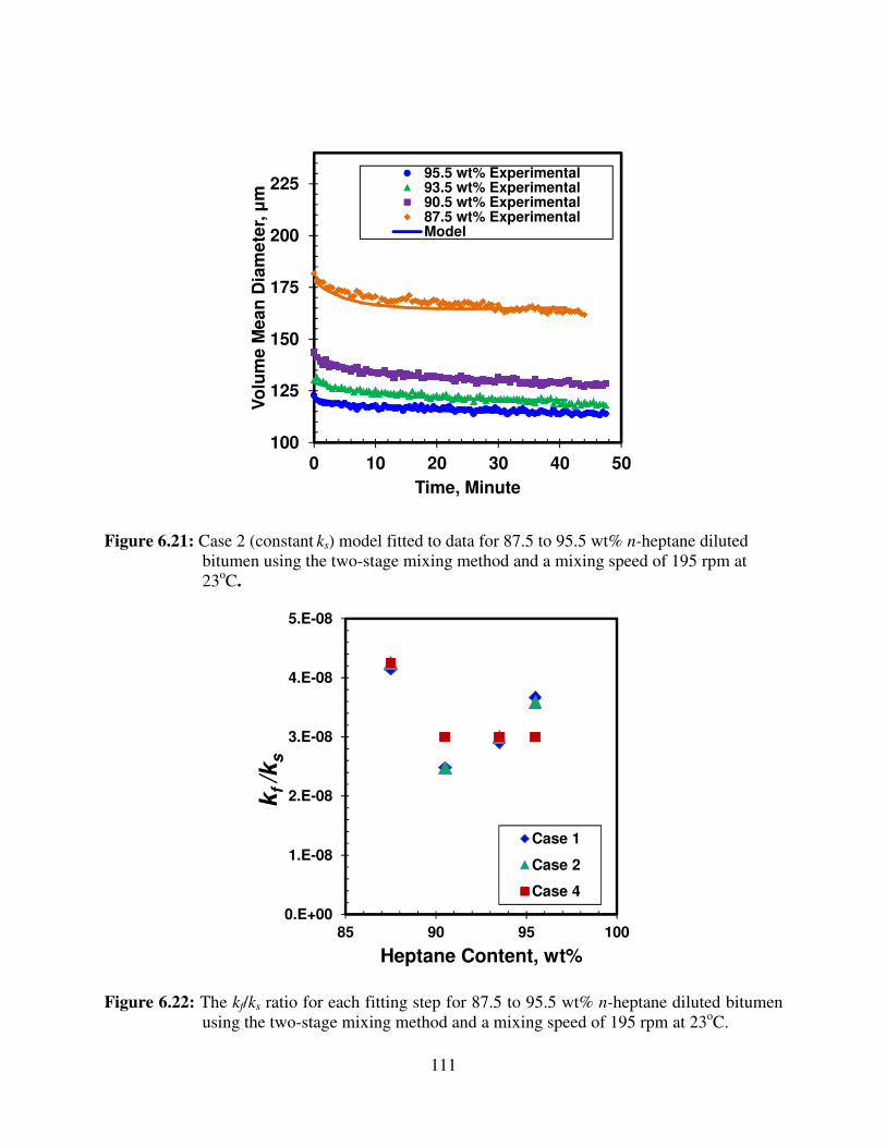
111
Figure 6.21: Case 2 (constant ks) model fitted to data for 87.5 to 95.5 wt% n-heptane diluted
bitumen using the two-stage mixing method and a mixing speed of 195 rpm at
23oC.
Figure 6.22: The kf/ks ratio for each fitting step for 87.5 to 95.5 wt% n-heptane diluted bitumen
using the two-stage mixing method and a mixing speed of 195 rpm at 23oC.
100
125
150
175
200
225
0 10 20 30 40 50
Vo
lum
e M
ea
n D
iam
ete
r, µ
m
Time, Minute
95.5 wt% Experimental93.5 wt% Experimental90.5 wt% Experimental87.5 wt% ExperimentalModel
0.E+00
1.E-08
2.E-08
3.E-08
4.E-08
5.E-08
85 90 95 100
kf /k
s
Heptane Content, wt%
Case 1
Case 2
Case 4
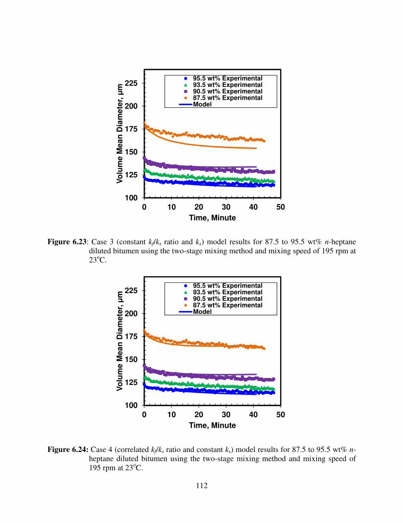
112
Figure 6.23: Case 3 (constant kf/ks ratio and ks) model results for 87.5 to 95.5 wt% n-heptane
diluted bitumen using the two-stage mixing method and mixing speed of 195 rpm at
23oC.
Figure 6.24: Case 4 (correlated kf/ks ratio and constant ks) model results for 87.5 to 95.5 wt% n-
heptane diluted bitumen using the two-stage mixing method and mixing speed of
195 rpm at 23oC.
100
125
150
175
200
225
0 10 20 30 40 50
Vo
lum
e M
ea
n D
iam
ete
r, µ
m
Time, Minute
95.5 wt% Experimental93.5 wt% Experimental90.5 wt% Experimental87.5 wt% ExperimentalModel
100
125
150
175
200
225
0 10 20 30 40 50
Vo
lum
e M
ea
n D
iam
ete
r, µ
m
Time, Minute
95.5 wt% Experimental93.5 wt% Experimental90.5 wt% Experimental87.5 wt% ExperimentalModel
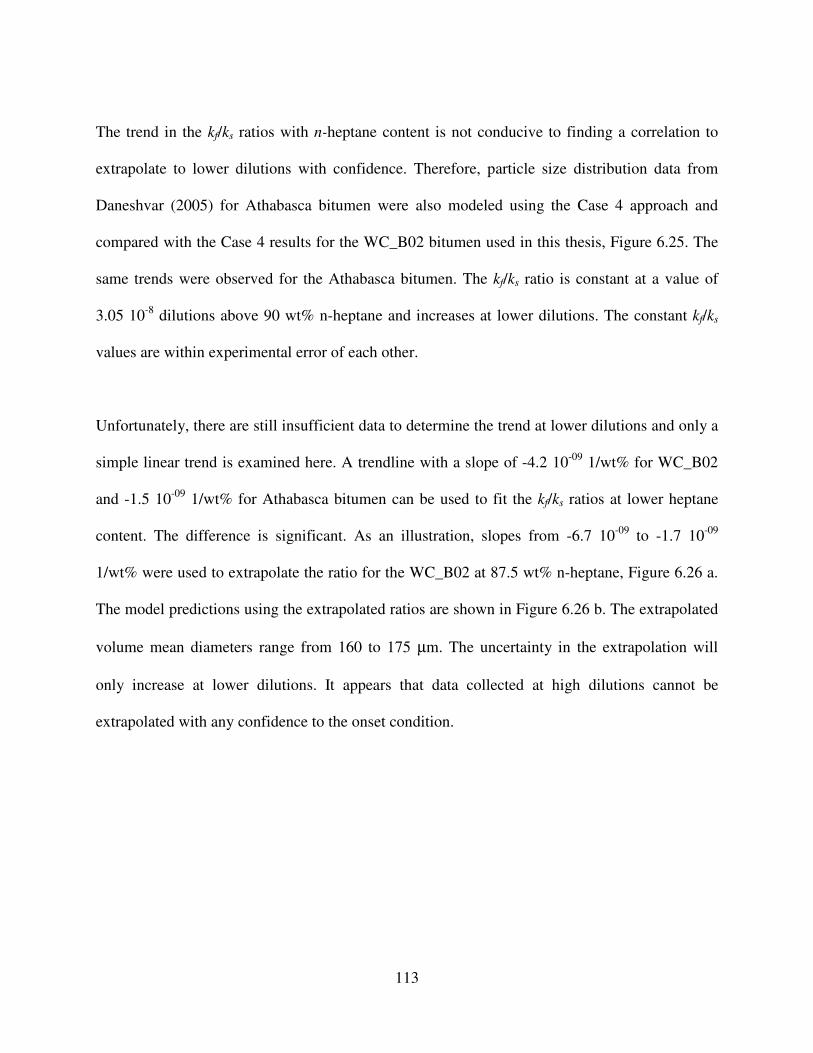
113
The trend in the kf/ks ratios with n-heptane content is not conducive to finding a correlation to
extrapolate to lower dilutions with confidence. Therefore, particle size distribution data from
Daneshvar (2005) for Athabasca bitumen were also modeled using the Case 4 approach and
compared with the Case 4 results for the WC_B02 bitumen used in this thesis, Figure 6.25. The
same trends were observed for the Athabasca bitumen. The kf/ks ratio is constant at a value of
3.05 10-8
dilutions above 90 wt% n-heptane and increases at lower dilutions. The constant kf/ks
values are within experimental error of each other.
Unfortunately, there are still insufficient data to determine the trend at lower dilutions and only a
simple linear trend is examined here. A trendline with a slope of -4.2 10-09
1/wt% for WC_B02
and -1.5 10-09
1/wt% for Athabasca bitumen can be used to fit the kf/ks ratios at lower heptane
content. The difference is significant. As an illustration, slopes from -6.7 10-09
to -1.7 10-09
1/wt% were used to extrapolate the ratio for the WC_B02 at 87.5 wt% n-heptane, Figure 6.26 a.
The model predictions using the extrapolated ratios are shown in Figure 6.26 b. The extrapolated
volume mean diameters range from 160 to 175 µm. The uncertainty in the extrapolation will
only increase at lower dilutions. It appears that data collected at high dilutions cannot be
extrapolated with any confidence to the onset condition.
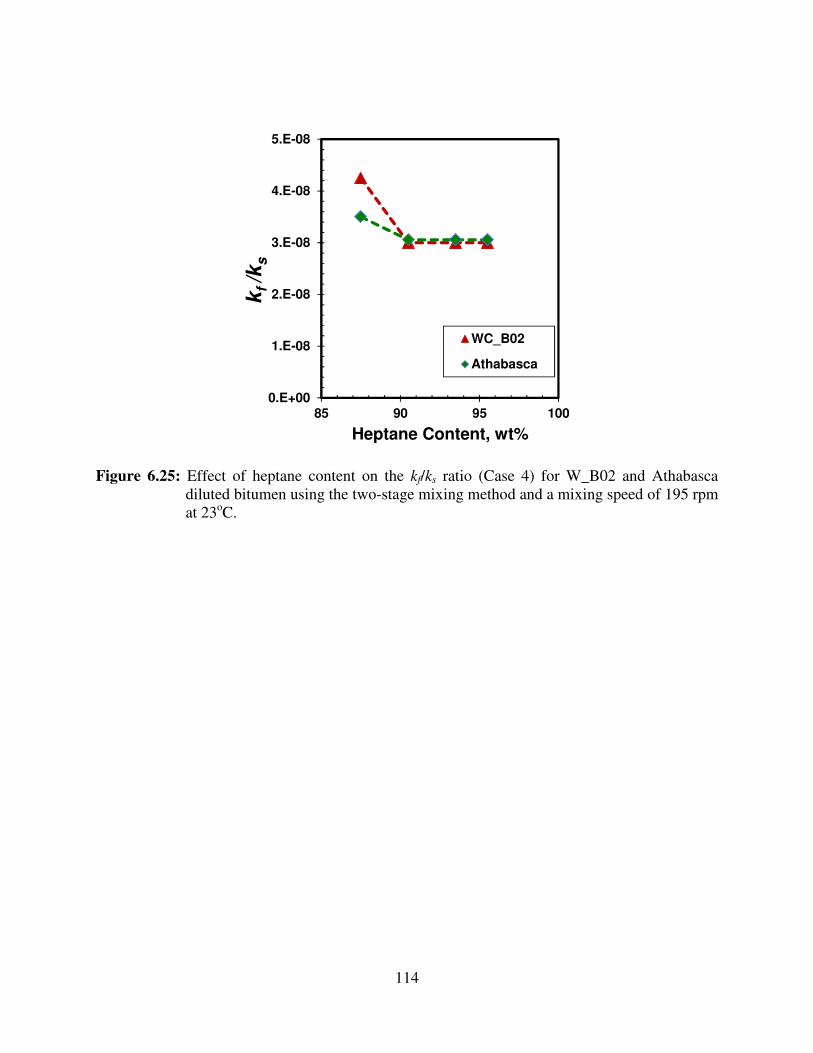
114
Figure 6.25: Effect of heptane content on the kf/ks ratio (Case 4) for W_B02 and Athabasca
diluted bitumen using the two-stage mixing method and a mixing speed of 195 rpm
at 23oC.
0.E+00
1.E-08
2.E-08
3.E-08
4.E-08
5.E-08
85 90 95 100
kf /k
s
Heptane Content, wt%
WC_B02
Athabasca
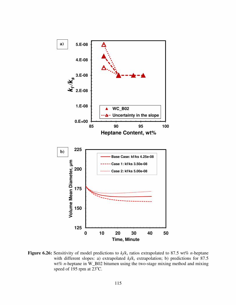
115
Figure 6.26: Sensitivity of model predictions to kf/ks ratios extrapolated to 87.5 wt% n-heptane
with different slopes: a) extrapolated kf/ks extrapolation; b) predictions for 87.5
wt% n-heptane in W_B02 bitumen using the two-stage mixing method and mixing
speed of 195 rpm at 23oC.
0.E+00
1.E-08
2.E-08
3.E-08
4.E-08
5.E-08
85 90 95 100
kf /k
s
Heptane Content, wt%
WC_B02
Uncertainty in the slope
125
150
175
200
225
0 10 20 30 40 50
Vo
lum
e M
ea
n D
iam
ete
r, µ
m
Time, Minute
Base Case: kf/ks 4.25e-08
Case 1: kf/ks 3.50e-08
Case 2: kf/ks 5.00e-08
a)
b)
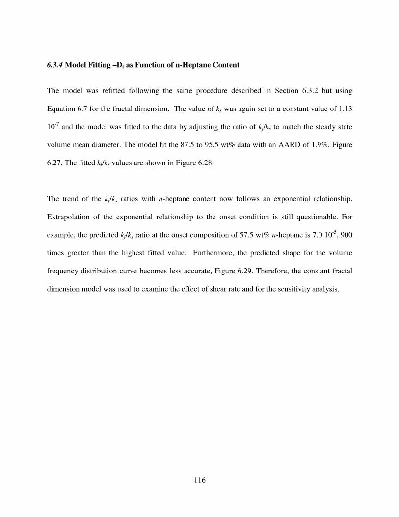
116
6.3.4 Model Fitting –Df as Function of n-Heptane Content
The model was refitted following the same procedure described in Section 6.3.2 but using
Equation 6.7 for the fractal dimension. The value of ks was again set to a constant value of 1.13
10-7
and the model was fitted to the data by adjusting the ratio of kf/ks to match the steady state
volume mean diameter. The model fit the 87.5 to 95.5 wt% data with an AARD of 1.9%, Figure
6.27. The fitted kf/ks values are shown in Figure 6.28.
The trend of the kf/ks ratios with n-heptane content now follows an exponential relationship.
Extrapolation of the exponential relationship to the onset condition is still questionable. For
example, the predicted kf/ks ratio at the onset composition of 57.5 wt% n-heptane is 7.0 10-5
, 900
times greater than the highest fitted value. Furthermore, the predicted shape for the volume
frequency distribution curve becomes less accurate, Figure 6.29. Therefore, the constant fractal
dimension model was used to examine the effect of shear rate and for the sensitivity analysis.
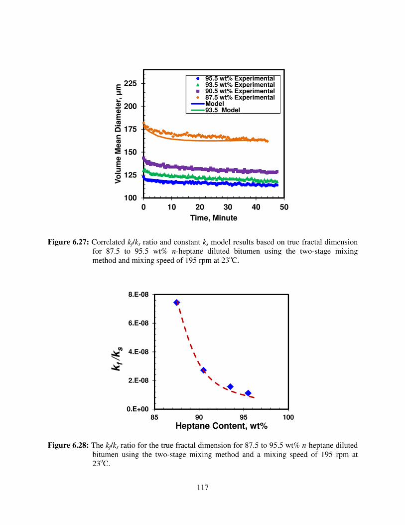
117
Figure 6.27: Correlated kf/ks ratio and constant ks model results based on true fractal dimension
for 87.5 to 95.5 wt% n-heptane diluted bitumen using the two-stage mixing
method and mixing speed of 195 rpm at 23oC.
Figure 6.28: The kf/ks ratio for the true fractal dimension for 87.5 to 95.5 wt% n-heptane diluted
bitumen using the two-stage mixing method and a mixing speed of 195 rpm at
23oC.
100
125
150
175
200
225
0 10 20 30 40 50
Vo
lum
e M
ea
n D
iam
ete
r, µ
m
Time, Minute
95.5 wt% Experimental93.5 wt% Experimental90.5 wt% Experimental87.5 wt% ExperimentalModel93.5 Model
0.E+00
2.E-08
4.E-08
6.E-08
8.E-08
85 90 95 100
kf /k
s
Heptane Content, wt%
118
Figure 6.29: Effect of adjusting Df on the volume frequency distribution for 87.5 wt% n-heptane
diluted bitumen using the two-stage mixing method and a mixing speed of 195 rpm
at 23oC.
6.3.5 Effect of Shear Conditions – Constant Df
This section investigates the effects of shear rate on the kf/ks ratio at various heptane contents.
Shear rates and Reynolds numbers were reported in Table 3.2. Figure 6.30 a plots the kf/ks ratio
versus the Reynolds number (Re) at each dilution ratio and mixing speed. Figure 6.30 b shows
that the same trends are observed for both Athabasca and WC_B02 bitumen. The kf/ks ratio
appears to decrease with increasing Reynolds number up to a Reynolds number of 12000 above
which the ratio becomes constant. In general, increasing shear is expected to increase shattering
rates relative to flocculation rates.
0
0.05
0.1
0.15
0.2
0.25
0.3
0.35
0.4
0.45
0.5
0 200 400 600
Vo
lum
eF
req
ue
nc
y %
pe
r B
ine
Siz
e
Bin Size µm
Measured
Df=2.42
Df=2.23
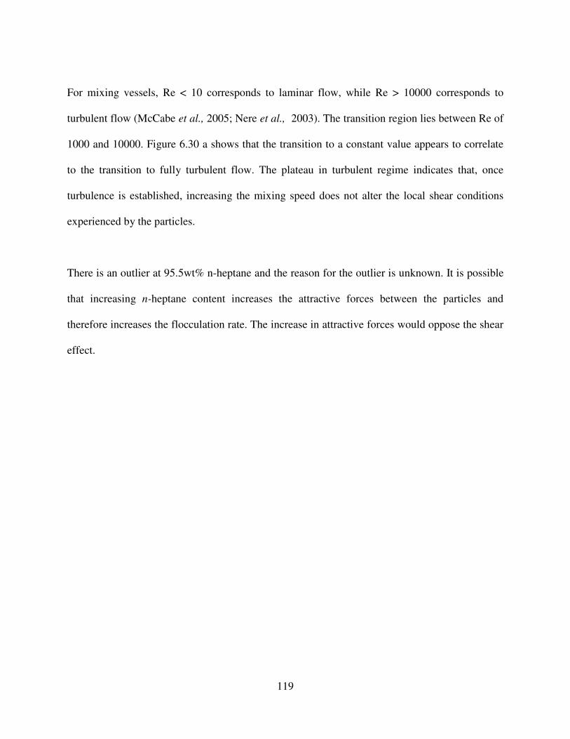
119
For mixing vessels, Re < 10 corresponds to laminar flow, while Re > 10000 corresponds to
turbulent flow (McCabe et al., 2005; Nere et al., 2003). The transition region lies between Re of
1000 and 10000. Figure 6.30 a shows that the transition to a constant value appears to correlate
to the transition to fully turbulent flow. The plateau in turbulent regime indicates that, once
turbulence is established, increasing the mixing speed does not alter the local shear conditions
experienced by the particles.
There is an outlier at 95.5wt% n-heptane and the reason for the outlier is unknown. It is possible
that increasing n-heptane content increases the attractive forces between the particles and
therefore increases the flocculation rate. The increase in attractive forces would oppose the shear
effect.
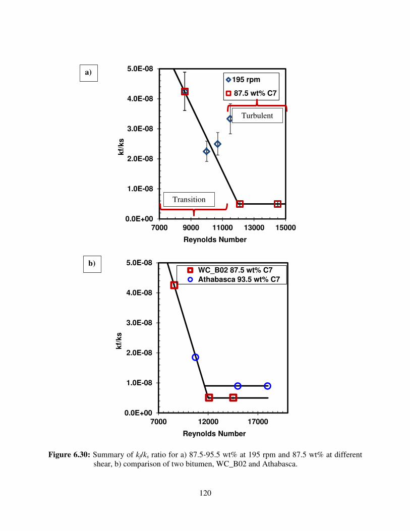
120
Figure 6.30: Summary of kf/ks ratio for a) 87.5-95.5 wt% at 195 rpm and 87.5 wt% at different
shear, b) comparison of two bitumen, WC_B02 and Athabasca.
0.0E+00
1.0E-08
2.0E-08
3.0E-08
4.0E-08
5.0E-08
7000 9000 11000 13000 15000
kf/
ks
Reynolds Number
195 rpm
87.5 wt% C7
0.0E+00
1.0E-08
2.0E-08
3.0E-08
4.0E-08
5.0E-08
7000 12000 17000
kf/
ks
Reynolds Number
WC_B02 87.5 wt% C7
Athabasca 93.5 wt% C7
Transition
Turbulent
a)
b)

121
6.3.6 Sensitivity to Model Parameters – Constant Df
The effect of the input parameters ks, β, λ, and Df as well as the bin size distribution on the
predicted volume mean diameter are presented. The sensitivities were performed on the 87.5
wt% n-heptane in bitumen using the two-stage mixing method and mixing speed of 195 rpm at
23oC case. The base input parameters for this case were provided in Table 6.1. The following
sensitivities were examined: ksx2 and ks/2, β ±0.1, λ ±0.1, and Df ±0.12.
Disintegration Constant, ks
The effect of adjusting disintegration reaction constant, ks, on the predicted steady state condition
is similar to adjusting the kf/ks ratio, Figure 6.31. However, the magnitude of ks also affects the
kinetics of flocculation (the shape of the curves in Figure 6.31 a). As expected, increasing ks by
factor of two decreases the volume mean diameter and increases the floc number count.
Increasing ks also leads to a more rapid approach to the steady state although it is difficult to see
in Figure 6.31 because the difference between the initial and steady state condition is also a
factor. Figure 6.32 shows that the volume frequency distributions are broader for higher volume
mean diameters but there is no other significant change in their shape.
Reaction Kernel Exponents, β and λ
The effects of adjusting β and λ were similar to that of changing the kf/ks ratio, as shown in
Figure 6.33 to 6.34. Therefore, there is likely little advantage in further tuning the model fits
using the reaction exponents.
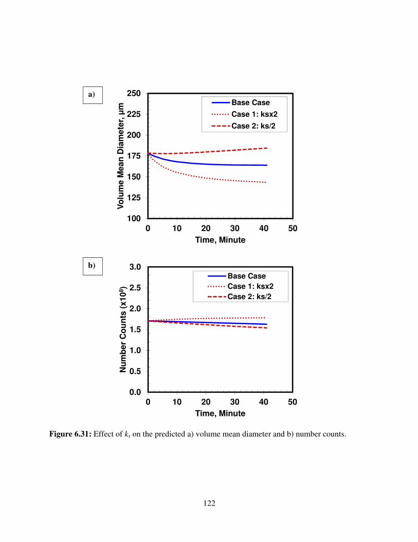
122
Figure 6.31: Effect of ks on the predicted a) volume mean diameter and b) number counts.
100
125
150
175
200
225
250
0 10 20 30 40 50
Vo
lum
e M
ea
n D
iam
ete
r, µ
m
Time, Minute
Base Case
Case 1: ksx2
Case 2: ks/2
0.0
0.5
1.0
1.5
2.0
2.5
3.0
0 10 20 30 40 50
Nu
mb
er
Co
un
ts (
x1
08)
Time, Minute
Base Case
Case 1: ksx2
Case 2: ks/2
a)
b)
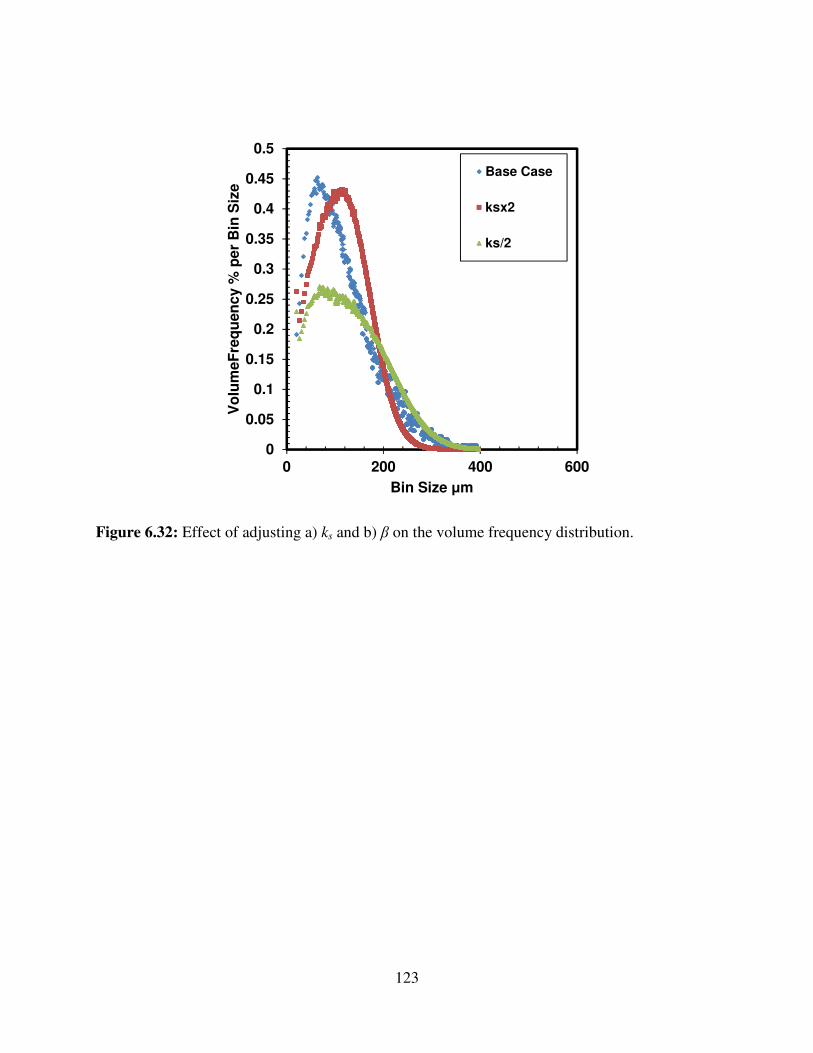
123
Figure 6.32: Effect of adjusting a) ks and b) β on the volume frequency distribution.
0
0.05
0.1
0.15
0.2
0.25
0.3
0.35
0.4
0.45
0.5
0 200 400 600
Vo
lum
eF
req
uen
cy %
pe
r B
in S
ize
Bin Size µm
Base Case
ksx2
ks/2
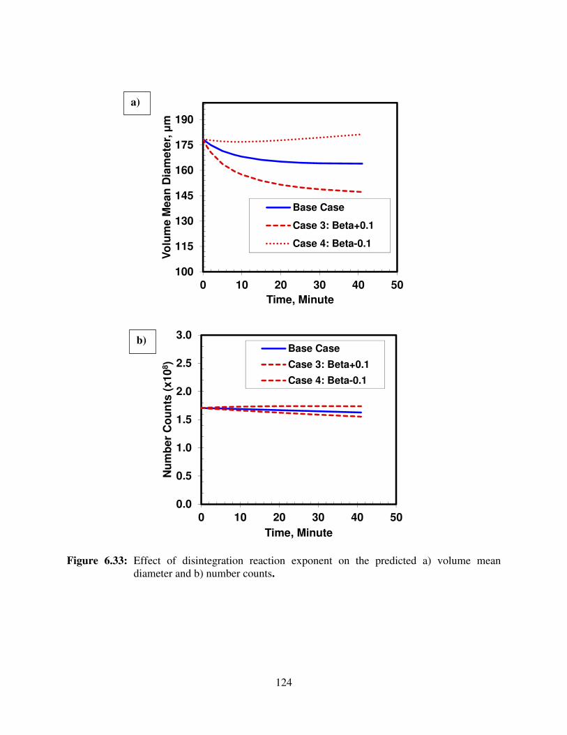
124
Figure 6.33: Effect of disintegration reaction exponent on the predicted a) volume mean
diameter and b) number counts.
100
115
130
145
160
175
190
0 10 20 30 40 50
Vo
lum
e M
ea
n D
iam
ete
r, µ
m
Time, Minute
Base Case
Case 3: Beta+0.1
Case 4: Beta-0.1
0.0
0.5
1.0
1.5
2.0
2.5
3.0
0 10 20 30 40 50
Nu
mb
er
Co
un
ts (
x1
08)
Time, Minute
Base Case
Case 3: Beta+0.1
Case 4: Beta-0.1
a)
b)
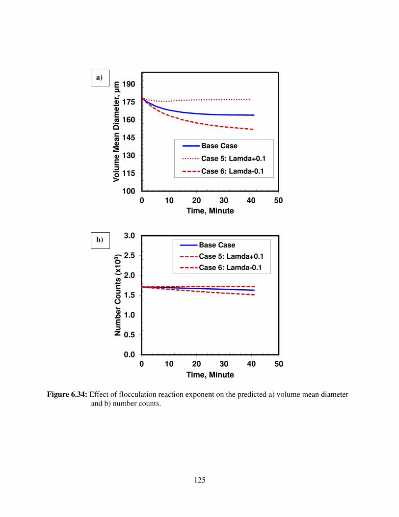
125
Figure 6.34: Effect of flocculation reaction exponent on the predicted a) volume mean diameter
and b) number counts.
100
115
130
145
160
175
190
0 10 20 30 40 50
Vo
lum
e M
ea
n D
iam
ete
r, µ
m
Time, Minute
Base Case
Case 5: Lamda+0.1
Case 6: Lamda-0.1
0.0
0.5
1.0
1.5
2.0
2.5
3.0
0 10 20 30 40 50
Nu
mb
er
Co
un
ts (
x1
08)
Time, Minute
Base Case
Case 5: Lamda+0.1
Case 6: Lamda-0.1
a)
b)
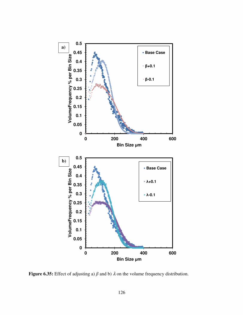
126
Figure 6.35: Effect of adjusting a) β and b) λ on the volume frequency distribution.
0
0.05
0.1
0.15
0.2
0.25
0.3
0.35
0.4
0.45
0.5
0 200 400 600
Vo
lum
eF
req
uen
cy %
per
Bin
Siz
e
Bin Size µm
Base Case
β+0.1
β-0.1
0
0.05
0.1
0.15
0.2
0.25
0.3
0.35
0.4
0.45
0.5
0 200 400 600
Vo
lum
eF
req
ue
ncy %
pe
r B
in S
ize
Bin Size µm
Base Case
λ+0.1
λ-0.1
a)
b)
127
Fractal Dimension, Df
The fractal dimension can potentially have a large impact on the model predictions. However,
the fractal dimension can be constrained to a small range. Recall, that the sediment volume of the
settled flocs is very sensitive to fractal dimension. For example, an increase of the fractal
dimension, Df, from 2.33 to 2.45 decreases the sediment volume from 35% to 25%. Therefore,
the sensitivity analysis was restricted to ±0.12. As expected, decreasing the fractal dimension
increases the number and size of the flocs, Figure 6.36. As noted previously, changing the fractal
dimension significantly alters the shape of the distributions, Figure 6.37. At lower fractal
dimension, the same number of particles gives a larger floc volume and the distribution tends to
become broad and flat. At higher fractal dimension, there are fewer but more compact flocs
giving a narrower distribution.
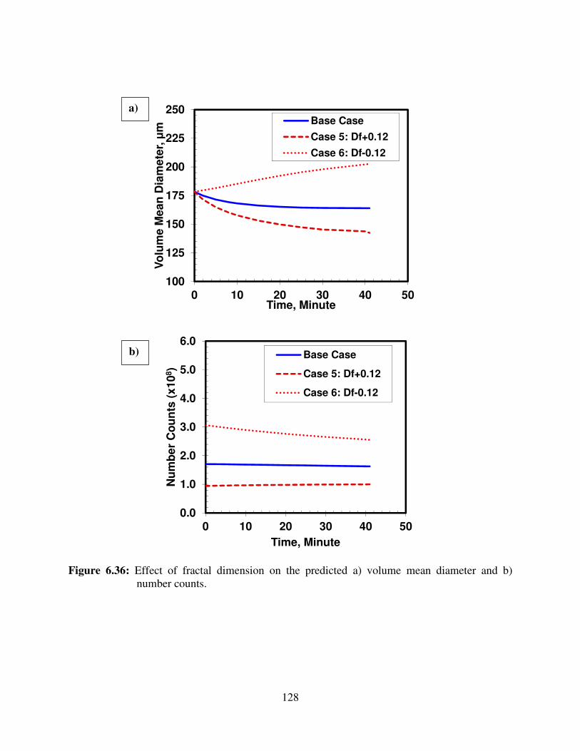
128
Figure 6.36: Effect of fractal dimension on the predicted a) volume mean diameter and b)
number counts.
100
125
150
175
200
225
250
0 10 20 30 40 50
Vo
lum
e M
ea
n D
iam
ete
r, µ
m
Time, Minute
Base Case
Case 5: Df+0.12
Case 6: Df-0.12
0.0
1.0
2.0
3.0
4.0
5.0
6.0
0 10 20 30 40 50
Nu
mb
er
Co
un
ts (
x1
08)
Time, Minute
Base Case
Case 5: Df+0.12
Case 6: Df-0.12
a)
b)
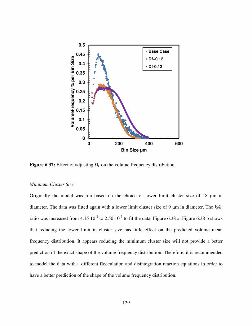
129
Figure 6.37: Effect of adjusting Df on the volume frequency distribution.
Minimum Cluster Size
Originally the model was run based on the choice of lower limit cluster size of 18 µm in
diameter. The data was fitted again with a lower limit cluster size of 9 µm in diameter. The kf/ks
ratio was increased from 4.15 10-8
to 2.50 10-7
to fit the data, Figure 6.38 a. Figure 6.38 b shows
that reducing the lower limit in cluster size has little effect on the predicted volume mean
frequency distribution. It appears reducing the minimum cluster size will not provide a better
prediction of the exact shape of the volume frequency distribution. Therefore, it is recommended
to model the data with a different flocculation and disintegration reaction equations in order to
have a better prediction of the shape of the volume frequency distribution.
0
0.05
0.1
0.15
0.2
0.25
0.3
0.35
0.4
0.45
0.5
0 200 400 600
Vo
lum
eF
req
ue
ncy %
pe
r B
in S
ize
Bin Size µm
Base Case
Df+0.12
Df-0.12
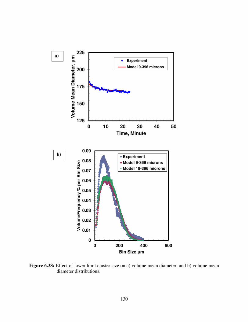
130
Figure 6.38: Effect of lower limit cluster size on a) volume mean diameter, and b) volume mean
diameter distributions.
125
150
175
200
225
0 10 20 30 40 50
Vo
lum
e M
ea
n D
iam
ete
r, µ
m
Time, Minute
Experiment
Model 9-396 microns
0
0.01
0.02
0.03
0.04
0.05
0.06
0.07
0.08
0.09
0 200 400 600
Vo
lum
eF
req
uen
cy %
per
Bin
Siz
e
Bin Size µm
Experiment
Model 9-369 microns
Model 18-396 microns
a)
b)
131
6.3.7 Summary
While asphaltene flocculation could not be measured near the onset conditions, data were
collected and modeled at higher dilutions. The main parameters controlling asphaltene
flocculation appear to be the particle concentration, the ratio of flocculation versus shattering
rates, and the fractal dimension of the flocs. In general, flocculation decreases at higher dilutions
because the particle concentration decreases. The driving force for flocculation (flocculation
versus shattering rate) appears to increase with increasing n-heptane content. The fractal
dimension decreases with increasing n-heptane content, leading to larger floc sizes for the same
number of particles. While the above trends could be extrapolated to near the onset condition, the
change in the parameter values is too great to have confidence in the extrapolation.
The effect of shear rate appears to be correlated to the Reynolds number. In transitional flow,
flocculation decreases as the Reynolds number increases. However, in turbulent flow,
flocculation becomes insensitive to changes in the Reynolds number. It appears that increasing
the mixing speed in turbulent conditions does not alter the local conditions encountered by the
flocs.
132
CHAPTER SEVEN: CONCLUSIONS AND RECOMMENDATIONS
The principal objectives of this thesis were to: 1) assess the role of oxygen in asphaltene
precipitation kinetics; 2) determine the kinetics of asphaltene precipitation from diluted
bitumen near the onset of precipitation, and; 3) investigate the kinetics of asphaltene
flocculation near the onset of precipitation. The main conclusions and recommendations from
this work are summarized below.
7.1 Conclusions
1. The onset determined from the gravimetric method was found to be in a good agreement
with microscopic observations. In air, the onset of asphaltene precipitation migrates to
lower solvent content over months and perhaps years, consistent with the observations of
Maqbool et al. (2009). In nitrogen, the onset of precipitation followed the same trends as
in air for the first 48 hours, but then became invariant over time.
2. Yields in air and nitrogen atmospheres were similar for the first 24 hours, but deviated
after 48 hours. The yields in air increase gradually over time over months while the yields
in nitrogen became invariant after 48 hours.
3. The long-term changes in onset and yield observed in air appear to be caused by
oxidation or oxygen-catalyzed polymerization. Hence, the yields in nitrogen must be used
to determine the kinetics of asphaltene precipitation in non-aerobic conditions. The shift
133
in onset and over the first 48 hours is not an oxygen related artifact, and is consistent with
a nucleation and growth process before reaching equilibrium. Asphaltene precipitation
kinetics follow a first order reaction model.
4. The particle size analyzer could not detect the particle size distribution in unadulterated
bitumen near the onset. The opacity and the stickiness of asphaltene particles resulted in
unreliable measurements at low dilutions. Therefore, data was collected at dilutions well
above the onset.
5. The method used to dilute bitumen with n-heptane can significantly change the
asphaltene floc size distribution and volume mean diameter. The one-stage mixing
method resulted in higher volume mean diameter both initially and at steady state. The
steady state is also reached quite slowly, whereas in two-stage mixing steady state is
reached more rapidly. Two-stage mixing reduces the potential for artifacts related to poor
mixing and therefore provides a better measure of the “true” flocculation kinetics.
6. For two-stage mixing, the asphaltene volume mean diameter decreases as the n-heptane
content increases. The decrease in the volume diameter with greater dilution correlates
with the decrease in individual particle concentrations.
7. An increase in the shear rate results in a decrease in the asphaltene volume mean
diameter, while the total number of asphaltene flocs in the mixture remained relatively
constant. This observation indicates that asphaltene flocs likely become more compact at
134
higher shear rates. Rastegari et al. (2004) and Daneshvar (2005) also reported that the
volume mean diameter decreases as the shear rate increases for the solutions of
asphaltene in the mixture of n-heptane and toluene.
8. The fractal dimension of the flocs was determined from the volume of a known mass of
asphaltene sediment and from image analysis of micrographs of settled flocs. The results
from both of these methods were consistent with an average fractal dimension of 2.3
±0.1.
9. The flocculation model was fitted the data at different dilutions. The main parameters
governing flocculation were the particle concentration, the fractal dimension, and the
magnitude and ratio of the flocculation and shattering rates, kf/ks. A constant value of the
shattering rate was sufficient to fit the data. Both the fractal dimension and the reaction
rate ratio could be correlated to the mass fraction of n-heptane. However, a long
extrapolation with a significant a change in parameter values is required to estimate the
behavior near the onset condition. Hence, the flocculation rates near the onset conditions
cannot be determined from the available data with any confidence.
10. The effect of shear rate on the kf/ks ratio at various heptane contents was investigated for
two different bitumen samples. The kf/ks ratio appears to decrease with increasing
Reynolds number up to 12000, above which the ratio becomes constant. The decrease in
the ratio corresponds to the transition zone, while the plateau corresponds to the
establishment of a turbulent zone.
135
7.2 Recommendations For Future Study
1. The thermodynamic onset was determined gravimetrically in a nitrogen atmosphere. It is
recommended to verify the thermodynamic onset with the microscopic techniques in
nitrogen atmosphere.
2. The onset of precipitation could not be determined in diluted WC-B03 bitumen with n-
pentane due to the existence of non-asphaltene particulates that obscured the onset. In
addition, the data from the gravimetric measurement was not consistent with the
microscopic method. Therefore, it is recommended to repeat the experiments with filtered
bitumen to reduce the scatter and improve the consistency of the results.
3. The onset of asphaltene precipitation occurs at higher n-heptane dilution when toluene is
present, allowing particle size distributions to be measured at lower n-heptane contents.
Therefore, for future work, it is recommended to investigate near onset kinetics in
toluene-diluted bitumen.
4. The population balance equation was derived assuming that only binary or two cluster
interactions are significant. This assumption is applicable only in dilute solutions. In
highly concentrated solutions more than two flocs can interact or flocculate at the same
time. Hence, it may be necessary to employ a new population balance equation including
those interaction terms.
136
5. The correlation established based on the trend in the kf/ks ratios with n-heptane content
was associated with high levels of uncertainty, largely due to the lack of data at lower
dilutions. Data collected at lower dilutions (for example in toluene diluted bitumen) could
be modeled to increase the level of confidence in the correlation.
6. The fractal dimension was assumed to be the same for all floc sizes and to remain
constant over time in the model. Considering a variable fractal dimension might improve
the performance of model.
7. For the commercial oil sand paraffinic froth treatment process, it is desirable to model the
flocculation of asphaltenes, solid particulates, and water droplets. It is recommended to
collect flocculation data for bitumen with emulsified water and solids using similar
procedures as described in this thesis. It is also recommended to measure floc sizes and
settling rates in a microscopic visualization cell. With this data, it may be possible to
extend the flocculation model to the commercial system.
137
4 REFERENCES
Agrawal, P., Schoeggl, F.F., Satyro, M.A., Taylor, S.D., Yarranton, H.W., 2012. Measurement
and modeling of the phase behavior of solvent diluted bitumens. Fluid Phase Equilibria
334, 51–64.
Agrawala, M., Yarranton, H.W., 2001. An asphaltene association model analogous to linear
polymerization. Ind. Eng. Chem. Res. 40, 4664–4672.
Angle, C.W., Long, Y., Hamza, H., Lue, L., 2006. Precipitation of asphaltenes from solvent-
diluted heavy oil and thermodynamic properties of solvent-diluted heavy oil solutions.
Fuel 85, 492–506. doi:10.1016/j.fuel.2005.08.009
Atkins, F.J., MacFadyen, A.J., 2008. A Resource Whose Time Has Come? The Alberta Oil
Sands as an Economic Resource. Energy J. 29, 77–98.
Barrett, P., Glennon, B., 1999. In-line FBRM Monitoring of Particle Size in Dilute Agitated
Suspensions. Part. Part. Syst. Charact. 16, 207–211.
Beck, J., Svrcek, W.Y., Yarranton, H.W., 2005. Hysteresis in Asphaltene Precipitation and
Redissolution. Energy Fuels 19, 944–947. doi:10.1021/ef049707n
Brawn, 2003. PRINCIPLES OF FLUID MIXING.
Browarzik, D., Laux, H., Rahimian, I., 1999a. Asphaltene flocculation in crude oil systems. Fluid
Phase Equilibria 154, 285–300. doi:10.1016/S0378-3812(98)00434-8
Browarzik, D., Laux, H., Rahimian, I., 1999b. Asphaltene flocculation in crude oil systems.
Fluid Phase Equilibria 154, 285–300. doi:10.1016/S0378-3812(98)00434-8
Buckley, J.S., 1999. Predicting the Onset of Asphaltene Precipitation from Refractive Index
Measurements. Energy Fuels 13, 328–332. doi:10.1021/ef980201c
Burke, N., Hobbs, R., Kashou, S., 1990. Measurement and Modeling of Asphaltene Precipitation
(includes associated paper 23831 ). J. Pet. Technol. 42. doi:10.2118/18273-PA
Castillo, J., Gutierrez, H., Ranaudo, M., Villarroel, O., 2010. Measurement of the Refractive
Index of Crude Oil and Asphaltene Solutions: Onset Flocculation Determination. Energy
Fuels 24, 492–495. doi:10.1021/ef900861d
Clark, K.A., Pasternack, D.S., 1932. Hot Water Seperation of Bitumen from Alberta Bituminous
Sand. Ind. Eng. Chem. 24, 1410–1416.
138
Daneshvar, S., 2005. Asphaltene Flocculation in Diluted Bitumen Systems (MSc.). University of
Calgary, Calgary.
De Clercq, B., Lant, P.A., Vanrolleghem, P.A., 2004. Focused beam reflectance technique for in
situ particle sizing in wastewater treatment settling tanks. J. Chem. Technol. Biotechnol.
79, 610–618.
Elimelech, M., Jia, X., Gregory, J., Williams, R., 1998. Particle deposition & aggregation:
measurement, modelling and simulation. Butterworth-Heinemann.
Eyssautier, J., Levitz, P., Espinat, D., Jestin, J., Gummel, J., Grillo, I., Barré, L., 2011. Insight
into asphaltene nanoaggregate structure inferred by small angle neutron and X-ray
scattering. J. Phys. Chem. B 115, 6827–6837.
Family, F., Meakin, P., Deutch, J.M., 1986. Kinetics of coagulation with fragmentation: scaling
behavior and fluctuations. Phys. Rev. Lett. 57, 727.
Fenistein, D., Barré, L., Broseta, D., Espinat, D., Livet, A., Roux, J.-N., Scarsella, M., 1998.
Viscosimetric and neutron scattering study of asphaltene aggregates in mixed
toluene/heptane solvents. Langmuir 14, 1013–1020.
Ferworn, K.A., Svrcek, W.Y., Mehrotra, A.K., 1993. Measurement of asphaltene particle size
distributions in crude oils diluted with n-heptane. Ind. Eng. Chem. Res. 32, 955–959.
doi:10.1021/ie00017a026
Gmachowski, L., n.d. Hydrodynamic Properties of Aggregates with Complex Structure.
Hamedi Rad, M., Tavakolian, M., Najafi, I., Ghazanfari, M.H., Taghikhani, V., Amani, M.,
2013. Modeling the kinetics of asphaltene flocculation in toluene–pentane systems for the
case of sonicated crude oils. Sci. Iran. 20, 611–616. doi:10.1016/j.scient.2012.12.018
Headen, T.F., Boek, E.S., Stellbrink, J., Scheven, U.M., 2009. Small angle neutron scattering
(SANS and V-SANS) study of asphaltene aggregates in crude oil. Langmuir ACS J. Surf.
Colloids 25, 422–428. doi:10.1021/la802118m
Heath, A.R., Fawell, P.D., Bahri, P.A., Swift, J.D., 2002. Estimating average particle size by
focused beam reflectance measurement (FBRM). Part. Part. Syst. Charact. 19, 84–95.
Higashitani, K., Okuhara, K., Hatade, S., 1992. Effects of magnetic fields on stability of
nonmagnetic ultrafine colloidal particles. J. Colloid Interface Sci. 152, 125–131.
doi:10.1016/0021-9797(92)90013-C
139
Hirschberg, A., DeJong, L.N.J., Schipper, B.A., Meijer, J.G., 1984. Influence of temperature and
pressure on asphaltene flocculation. Soc. Pet. Eng. J. 24, 283–293.
Hoepfner, M.P., Vilas Bôas Fávero, C., Haji-Akbari, N., Fogler, H.S., 2013. The Fractal
Aggregation of Asphaltenes. Langmuir.
Hu, Y.-F., Guo, T.-M., 2001. Effect of temperature and molecular weight of n-alkane
precipitants on asphaltene precipitation. Fluid Phase Equilibria 192, 13–25.
doi:10.1016/S0378-3812(01)00619-7
Kempkes, M., Eggers, J., Mazzotti, M., 2008. Measurement of particle size and shape by FBRM
and in situ microscopy. Chem. Eng. Sci. 63, 4656–4675.
Kim, S.T., Boudh-Hir, M.-E., Mansoori, G.A., 1990. The Role of Asphaltene in Wettability
Reversal . Society of Petroleum Engineers. doi:10.2118/20700-MS
Kinsner, W., 2005. A unified approach to fractal dimensions, in: Cognitive Informatics,
2005.(ICCI 2005). Fourth IEEE Conference on. IEEE, pp. 58–72.
Kotlyar, L.S., Sparks, B.D., Woods, J.R., Raymond, S., Le Page, Y., Shelfantook, W., 1998.
Distribution and types of solids associated with bitumen. Pet. Sci. Technol. 16, 1–19.
Kraiwattanawong, K., Fogler, H.S., Gharfeh, S.G., Singh, P., Thomason, W.H., Chavadej, S.,
2007. Thermodynamic solubility models to predict asphaltene instability in live crude
oils. Energy Fuels 21, 1248–1255.
Kraiwattanawong, K., Fogler, H.S., Gharfeh, S.G., Singh, P., Thomason, W.H., Chavadej, S.,
2009. Effect of asphaltene dispersants on aggregate size distribution and growth. Energy
Fuels 23, 1575–1582.
Mangold, M., 2012. Use of a Kalman filter to reconstruct particle size distributions from FBRM
measurements. Chem. Eng. Sci. 70, 99–108. doi:10.1016/j.ces.2011.05.052
Maqbool, T., Balgoa, A.T., Fogler, H.S., 2009. Revisiting asphaltene precipitation from crude
oils: A case of neglected kinetic effects. Energy Fuels 23, 3681–3686.
Maqbool, T., Raha, S., Hoepfner, M.P., Fogler, H.S., 2011. Modeling the aggregation of
asphaltene nanoaggregates in crude oil- precipitant systems. Energy Fuels 25, 1585–
1596.
Mason, T.G., Lin, M.Y., 2003. Time-resolved small angle neutron scattering measurements of
asphaltene nanoparticle aggregation kinetics in incompatible crude oil mixtures. J. Chem.
Phys. 119, 565.
140
McCabe, W.L., Smith, J., Harriott, P., 2005. Unit Operations of Chemical Engineering.
McGraw-Hill Education.
Mousavi-Dehghani, S.., Riazi, M.., Vafaie-Sefti, M., Mansoori, G.., 2004. An analysis of
methods for determination of onsets of asphaltene phase separations. J. Pet. Sci. Eng. 42,
145–156. doi:10.1016/j.petrol.2003.12.007
Mullins, O.C., Sabbah, H., Eyssautier, J., Pomerantz, A.E., Barré, L., Andrews, A.B., Ruiz-
Morales, Y., Mostowfi, F., McFarlane, R., Goual, L., Lepkowicz, R., Cooper, T.,
Orbulescu, J., Leblanc, R.M., Edwards, J., Zare, R.N., 2012. Advances in Asphaltene
Science and the Yen–Mullins Model. Energy Fuels 26, 3986–4003.
doi:10.1021/ef300185p
Mullins, O.C., Sheu, E.Y., 1998. Structures and dynamics of asphaltenes. Springer.
Najafi, I., Mousavi, S.M.R., Ghazanfari, M.H., Ghotbi, C., Ramazani, A., Kharrat, R., Amani,
M., 2011. Quantifying the Role of Ultrasonic Wave Radiation on Kinetics of Asphaltene
Aggregation in a Toluene–Pentane Mixture. Pet. Sci. Technol. 29, 966–974.
doi:10.1080/10916460903394144
Nere, N.K., Patwardhan, A.W., Joshi, J.B., 2003. Liquid-phase mixing in stirred vessels:
turbulent flow regime. Ind. Eng. Chem. Res. 42, 2661–2698.
Nielsen, B.B., Svrcek, W.Y., Mehrotra, A.K., 1994. Effects of temperature and pressure on
asphaltene particle size distributions in crude oils diluted with n-pentane. Ind. Eng.
Chem. Res. 33, 1324–1330.
Rahmani, N.H.G., Dabros, T., Masliyah, J.H., 2004. Evolution of asphaltene floc size
distribution in organic solvents under shear. Chem. Eng. Sci. 59, 685–697.
doi:10.1016/j.ces.2003.10.017
Rahmani, N.H.G., Dabros, T., Masliyah, J.H., 2005. Fractal structure of asphaltene aggregates. J.
Colloid Interface Sci. 285, 599–608. doi:10.1016/j.jcis.2004.11.068
Rastegari, K., Svrcek, W.Y., Yarranton, H.W., 2004. Kinetics of Asphaltene Flocculation. Ind.
Eng. Chem. Res. 43, 6861–6870. doi:10.1021/ie049594v
Romanova, U.G., Valinasab, M., Stasiuk, E.N., Yarranton, H.W., Schramm, L.L., Shelfantook,
W.E., 2006. The effect of oil sands bitumen extraction conditions on froth treatment
performance. J. Can. Pet. Technol. 45, 36–45.
141
Sanford, E.C., Seyer, F.A., 1979. PROCESSIBILITY OF ATHABASCA TAR SAND USING A
BATCH EXTRACTION UNIT-ROLE OF NAOH. CIM Bull. 72, 164–169.
Saryazdi, F., Motahhari, H., Schoeggl, F.F., Taylor, S.D., Yarranton, H.W., 2013. Density of
Hydrocarbon Mixtures and Bitumen Diluted with Solvents and Dissolved Gases. Energy
Fuels 27, 3666–3678. doi:10.1021/ef400330j
Sathe, D., Sawant, K., Mondkar, H., Naik, T., Deshpande, M., 2010. Monitoring temperature
effect on the polymorphic transformation of acitretin using FBRM- Lasentec. Org.
Process Res. Dev. 14, 1373–1378.
Savvidis, T.G., Fenistein, D., Barré, L., Behar, E., 2001. Aggregated structure of flocculated
asphaltenes. AIChE J. 47, 206–211.
Sheu, E., Long, Y., Hamza, H., 2007. Asphaltene Self-Association and Precipitation in
Solvents—AC Conductivity Measurements, in: Mullins, O.C., Sheu, E.Y., Hammami, A.,
Marshall, A.G. (Eds.), Asphaltenes, Heavy Oils, and Petroleomics. Springer New York,
pp. 259–277.
Speight, J.G., 2006. The Chemistry and Technology of Petroleum, Fourth Edition. CRC Press.
Taylor, W.F., Frankenfeld, J.W., 1978. Deposit Formation from Deoxygenated Hydrocarbons. 3.
Effects of Trace Nitrogen and Oxygen Compounds. Ind. Eng. Chem. Prod. Res. Dev. 17,
86–90.
The MathWorks, Inc. Matlab Version 2014 a, " Matlab User's Mannual" Calgary, Canada 2014.
Uhl, V.W., Gray, J.B., 1986. Mixing: theory and practice. Volume III.
Wattana, P., Wojciechowski, D.J., Bolaños, G., Fogler, H.S., 2003. Study of Asphaltene
Precipitation Using Refractive Index Measurement. Pet. Sci. Technol. 21, 591–613.
doi:10.1081/LFT-120018541
Welt, J., Lee, W., Krambeck, F.J., 1977. Catalyst attrition and deactivation in fluid catalytic
cracking system. Chem. Eng. Sci. 32, 1211–1218.
Wiehe, I.A., Yarranton, H.W., Akbarzadeh, K., Rahimi, P.M., Teclemariam, A., 2005. The
paradox of asphaltene precipitation with normal paraffins. Energy Fuels 19, 1261–1267.
Wilson, D.I., Watkinson, A.P., 1996. A study of autoxidation reaction fouling in heat
exchangers. Can. J. Chem. Eng. 74, 236–246.
142
Wu, J., Graham, L.J., Noui Mehidi, N., 2006. Estimation of agitator flow shear rate. AIChE J.
52, 2323–2332. doi:10.1002/aic.10857
Yarranton, H.W., 2005. Asphaltene Self‐Association. J. Dispers. Sci. Technol. 26, 5–8.
doi:10.1081/DIS-200040234
Yarranton, H.W., Alboudwarej, H., Jakher, R., 2000. Investigation of Asphaltene Association
with Vapor Pressure Osmometry and Interfacial Tension Measurements. Ind. Eng. Chem.
Res. 39, 2916–2924. doi:10.1021/ie000073r
Yen, T.F., Chilingarian, G.V., 2000. Asphaltenes and Asphalts, 2. Elsevier.
Yen, T.F., Erdman, J.G., Pollack, S.S., 1961. Investigation of the structure of petroleum
asphaltenes by X-ray diffraction. Anal. Chem. 33, 1587–1594.
Zhang, R., Khalizov, A., Wang, L., Hu, M., Xu, W., 2011. Nucleation and growth of
nanoparticles in the atmosphere. Chem. Rev. 112, 1957–2011.
143
APPENDIX A: AVERAGE ABSOLUTE RELATIVE DEVIATION
The repeatability analysis for the asphaltene precipitation measurements are shown in Chapter 4.
The mean, µ, is given by:
) = ∑ UAVA��W (A.1)
Where yi is the experimental measured value and n is the number of measurements or repeats.
The sample variance, s, was calculated based on the variance for all of the measurements and is
given by:
X = Y∑ (UA�F)DVA��M�� (A.2)
Where m is the number of variances determined for the measurement. The variance of the
property measurements is then estimated using a chi-square distribution as follows:
Z = Y [D7D(W��) (A.3)
Where \� is the Chi-square variable (from statistical tables) and X� is the population standard
deviation. The 90% confidence interval for any measurement is determined as 1.645 Z.
The Average Absolute Relative Deviation (AARD) between the predicted ]�∗ and experimentally
measured values ]� are expressed by Equation A.4:
_`+ = ]�∗ − ]� (A.4)
The Average Absolute Deviation or AAD is given by Equation A.5:
aa2 = �W∑ |]�∗ − ]�|W� (A.5)

144
and the Absolute Average Relative Deviation is given by:
aa42 = �W ∑ cUA
∗�UAUA
cW� (A.6)
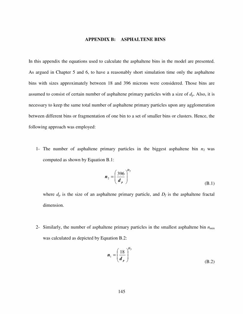
145
APPENDIX B: ASPHALTENE BINS
In this appendix the equations used to calculate the asphaltene bins in the model are presented.
As argued in Chapter 5 and 6, to have a reasonably short simulation time only the asphaltene
bins with sizes approximately between 18 and 396 microns were considered. Those bins are
assumed to consist of certain number of asphaltene primary particles with a size of dp. Also, it is
necessary to keep the same total number of asphaltene primary particles upon any agglomeration
between different bins or fragmentation of one bin to a set of smaller bins or clusters. Hence, the
following approach was employed:
1- The number of asphaltene primary particles in the biggest asphaltene bin n2 was
computed as shown by Equation B.1:
fD
pdn
=
3962
(B.1)
where dp is the size of an asphaltene primary particle, and Df is the asphaltene fractal
dimension.
2- Similarly, the number of asphaltene primary particles in the smallest asphaltene bin nmin
was calculated as depicted by Equation B.2:
fD
pdn
=
181
(B.2)
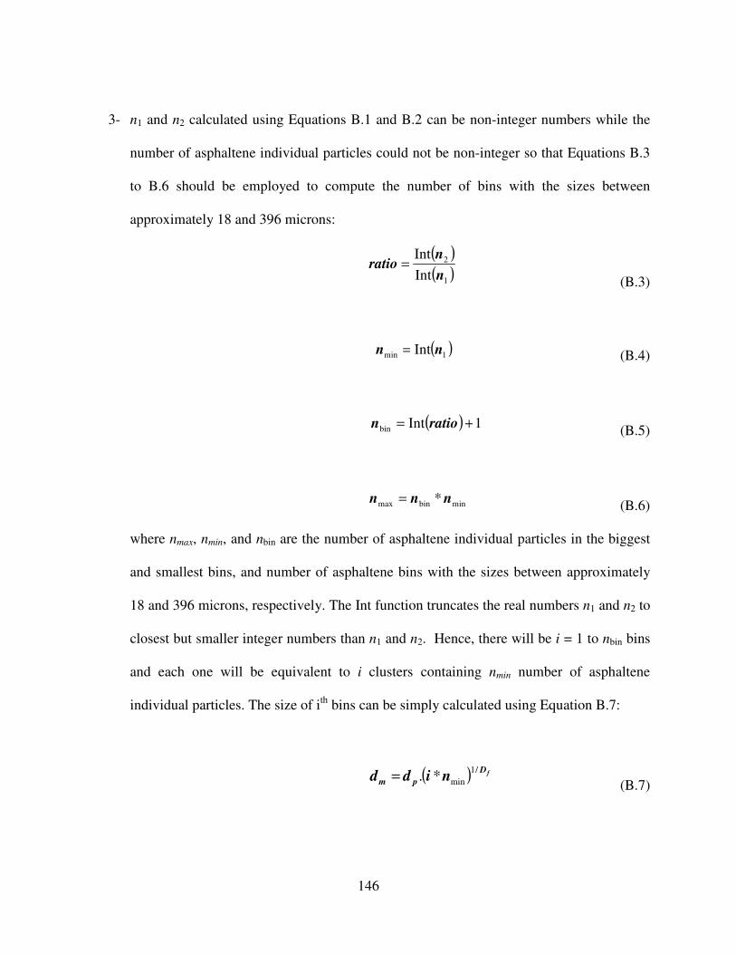
146
3- n1 and n2 calculated using Equations B.1 and B.2 can be non-integer numbers while the
number of asphaltene individual particles could not be non-integer so that Equations B.3
to B.6 should be employed to compute the number of bins with the sizes between
approximately 18 and 396 microns:
( )( )1
2
Int
Int
n
nratio =
(B.3)
( )1min Int nn = (B.4)
( ) 1Intbin += ration (B.5)
minbinmax * nnn = (B.6)
where nmax, nmin, and nbin are the number of asphaltene individual particles in the biggest
and smallest bins, and number of asphaltene bins with the sizes between approximately
18 and 396 microns, respectively. The Int function truncates the real numbers n1 and n2 to
closest but smaller integer numbers than n1 and n2. Hence, there will be i = 1 to nbin bins
and each one will be equivalent to i clusters containing nmin number of asphaltene
individual particles. The size of ith
bins can be simply calculated using Equation B.7:
( ) fD
pm nidd/1
min*.= (B.7)