Embed Size (px)
Citation preview
University of São Paulo“Luiz de Queiroz” College of Agriculture
Contributions to the analysis of dispersed count data
Eduardo Elias Ribeiro Junior
Dissertation presented to obtain the degree of Masterin Science. Area: Statistics and Agricultural Experi-mentation
Piracicaba2019
Eduardo Elias Ribeiro JuniorBachelor in Statistics
Contributions to the analysis of dispersed count dataversão revisada de acordo com a resolução CoPGr 6018 de 2011
Advisor:Profa. Dra. CLARICE GARCIA BORGES DEMÉTRIO
Dissertation presented to obtain the degree of Master inScience. Area: Statistics and Agricultural Experimenta-tion
Piracicaba2019

2
Dados Internacionais de Catalogação na PublicaçãoDIVISÃO DE BIBLIOTECA - DIBD/ESALQ/USP
Ribeiro Junior, Eduardo EliasContributions to the analysis of dispersed count data / Eduardo Elias
Ribeiro Junior. – – versão revisada de acordo com a resolução CoPGr 6018de 2011. – – Piracicaba, 2019 .
82 p.
Dissertação (Mestrado) – – USP / Escola Superior de Agricultura “Luizde Queiroz”.
1. Dados de contagens 2. Dispersão variável 3. Inferência baseada emverossimilhança 4. Modelos probabilísticos discretos 5. Subdispersão 6. Su-perdipersão . I. Título.

To my family

5
CONTENTS
Resumo . . . . . . . . . . . . . . . . . . . . . . . . . . . . . . . . . . . . . . . 7Abstract . . . . . . . . . . . . . . . . . . . . . . . . . . . . . . . . . . . . . . . 8
1 General introduction . . . . . . . . . . . . . . . . . . . . . . . . . . . . . . . . 9References . . . . . . . . . . . . . . . . . . . . . . . . . . . . . . . . . . . . . . . . 10
2 Motivating studies . . . . . . . . . . . . . . . . . . . . . . . . . . . . . . . . . 132.1 Artificial defoliation in cotton phenology . . . . . . . . . . . . . . . . . . . . . . . . 132.2 Soil moisture and potassium fertilization on soybean culture . . . . . . . . . . . . . 142.3 Toxicity of nitrofen in aquatic systems . . . . . . . . . . . . . . . . . . . . . . . . . 152.4 Annona mucosa in control of stored maize peast . . . . . . . . . . . . . . . . . . . . 162.5 Alternative substrats for bromeliad production . . . . . . . . . . . . . . . . . . . . . 16
References . . . . . . . . . . . . . . . . . . . . . . . . . . . . . . . . . . . . . . . . 173 Reparametrization of COM-Poisson regression models . . . . . . . . . . . . . 19
Abstract . . . . . . . . . . . . . . . . . . . . . . . . . . . . . . . . . . . . . . . . . 193.1 Introduction . . . . . . . . . . . . . . . . . . . . . . . . . . . . . . . . . . . . . . . 193.2 Background . . . . . . . . . . . . . . . . . . . . . . . . . . . . . . . . . . . . . . . 203.3 Reparametrized COM-Poisson regression model . . . . . . . . . . . . . . . . . . . . 223.4 Estimation and inference . . . . . . . . . . . . . . . . . . . . . . . . . . . . . . . . 243.5 Simulation study . . . . . . . . . . . . . . . . . . . . . . . . . . . . . . . . . . . . . 253.6 Case studies . . . . . . . . . . . . . . . . . . . . . . . . . . . . . . . . . . . . . . . 293.6.1 Artificial defoliation in cotton phenology . . . . . . . . . . . . . . . . . . . . . . . . 293.6.2 Soil moisture and potassium doses on soybean culture . . . . . . . . . . . . . . . . . 313.6.3 Assessing toxicity of nitrofen in aquatic systems . . . . . . . . . . . . . . . . . . . . 323.7 Concluding remarks . . . . . . . . . . . . . . . . . . . . . . . . . . . . . . . . . . . 35
References . . . . . . . . . . . . . . . . . . . . . . . . . . . . . . . . . . . . . . . . 364 A review of flexible models for dispersed count data . . . . . . . . . . . . . . 39
Abstract . . . . . . . . . . . . . . . . . . . . . . . . . . . . . . . . . . . . . . . . . 394.1 Introduction . . . . . . . . . . . . . . . . . . . . . . . . . . . . . . . . . . . . . . . 394.2 Background . . . . . . . . . . . . . . . . . . . . . . . . . . . . . . . . . . . . . . . 404.2.1 COM-Poisson distribution . . . . . . . . . . . . . . . . . . . . . . . . . . . . . . . . 404.2.2 Gamma-count distribution . . . . . . . . . . . . . . . . . . . . . . . . . . . . . . . . 414.2.3 Discrete Weibull distribution . . . . . . . . . . . . . . . . . . . . . . . . . . . . . . 424.2.4 Generalized Poisson distribution . . . . . . . . . . . . . . . . . . . . . . . . . . . . . 434.2.5 Double Poisson distribution . . . . . . . . . . . . . . . . . . . . . . . . . . . . . . . 434.2.6 Poisson-Tweedie distribution . . . . . . . . . . . . . . . . . . . . . . . . . . . . . . 444.3 Comparing count distributions . . . . . . . . . . . . . . . . . . . . . . . . . . . . . 454.4 Regression models and estimation . . . . . . . . . . . . . . . . . . . . . . . . . . . 484.5 Data analyses . . . . . . . . . . . . . . . . . . . . . . . . . . . . . . . . . . . . . . 504.5.1 Sitophilus zeamaus experiment . . . . . . . . . . . . . . . . . . . . . . . . . . . . . 504.5.2 Bromeliad experiment . . . . . . . . . . . . . . . . . . . . . . . . . . . . . . . . . . 514.6 Discussion . . . . . . . . . . . . . . . . . . . . . . . . . . . . . . . . . . . . . . . . 55
6
References . . . . . . . . . . . . . . . . . . . . . . . . . . . . . . . . . . . . . . . . 565 COM-Poisson models with varying dispersion . . . . . . . . . . . . . . . . . . 59
Abstract . . . . . . . . . . . . . . . . . . . . . . . . . . . . . . . . . . . . . . . . . 595.1 Introduction . . . . . . . . . . . . . . . . . . . . . . . . . . . . . . . . . . . . . . . 595.2 Double generalized linear models . . . . . . . . . . . . . . . . . . . . . . . . . . . . 605.3 Modeling mean and dispersion COM-Poisson . . . . . . . . . . . . . . . . . . . . . . 615.4 Estimation and inference . . . . . . . . . . . . . . . . . . . . . . . . . . . . . . . . 625.5 Simulation study . . . . . . . . . . . . . . . . . . . . . . . . . . . . . . . . . . . . . 635.6 Applications and discussion . . . . . . . . . . . . . . . . . . . . . . . . . . . . . . . 655.6.1 Analysis of nitrofen experiment . . . . . . . . . . . . . . . . . . . . . . . . . . . . . 655.6.2 Analysis of soybean experiment . . . . . . . . . . . . . . . . . . . . . . . . . . . . . 685.7 Final remarks . . . . . . . . . . . . . . . . . . . . . . . . . . . . . . . . . . . . . . 69
References . . . . . . . . . . . . . . . . . . . . . . . . . . . . . . . . . . . . . . . . 716 Final considerations . . . . . . . . . . . . . . . . . . . . . . . . . . . . . . . . . 73
References . . . . . . . . . . . . . . . . . . . . . . . . . . . . . . . . . . . . . . . . 73Appendix . . . . . . . . . . . . . . . . . . . . . . . . . . . . . . . . . . . . . . 75Appendix A: R packages and computational routines . . . . . . . . . . . . . . . . . . 75Bibliography . . . . . . . . . . . . . . . . . . . . . . . . . . . . . . . . . . . . . 79
7
RESUMO
Contribuições à análise de dados de contagem
Em diversos estudos agrícolas e biológicos, a variável resposta é um número inteiro não neg-ativo que desejamos explicar ou analisar em termos de um conjunto de covariáveis. Difer-entemente do modelo linear Gaussiano, a variável resposta é discreta com distribuição deprobabilidade definida apenas em valores do conjunto dos naturais. O modelo Poisson é omodelo padrão para dados em forma de contagens. No entanto, as suposições desse mod-elo forçam que a média seja igual a variância, o que pode ser implausível em muitas apli-cações. Motivado por conjuntos de dados experimentais, este trabalho teve como objetivodesenvolver métodos mais realistas para a análise de contagens. Foi proposta uma novareparametrização da distribuição COM-Poisson e explorados modelos de regressão baseadosnessa distribuição. Uma extensão desse modelo para permitir que a dispersão, assim comoa média, dependa de covariáveis, foi proposta. Um conjunto de modelos para contagens,nomeadamente COM-Poisson, Gamma-count, Weibull discreto, Poisson generalizado, duploPoisson e Poisson-Tweedie, foi revisado e comparado, considerando os índices de dispersão,inflação de zero e cauda pesada, juntamente com os resultados de análises de dados. Asrotinas computacionais desenvolvidas nesta dissertação foram organizadas em dois pacotesR disponíveis no GitHub.
Keywords: Dados de contagens, Dispersão variável, Inferência baseada em verossimilhança,Modelos probabilísticos discretos, Subdispersão, Superdipersão.
8
ABSTRACT
Contributions to the analysis of dispersed count data
In many agricultural and biological contexts, the response variable is a nonnegative integervalue which we wish to explain or analyze in terms of a set of covariates. Unlike the Gaus-sian linear model, the response variable is discrete with a distribution that places probabilitymass at natural numbers only. The Poisson regression is the standard model for count data.However, assumptions of this model forces the equality between mean and variance, whichmay be implausible in many applications. Motivated by experimental data sets, this workintended to develop more realistic methods for the analysis of count data. We proposed anovel parametrization of the COM-Poisson distribution and explored the regression modelsbased on it. We extended the model to allow the dispersion, as well as the mean, dependingon covariates. A set of count statistical models, namely COM-Poisson, Gamma-count, dis-crete Weibull, generalized Poisson, double Poisson and Poisson-Tweedie, was reviewed andcompared, considering the dispersion, zero-inflation, and heavy tail indexes, together withthe results of data analyzes. The computational routines developed in this dissertation wereorganized in two R packages available on GitHub.
Keywords: Count data, Discrete probability models, Likelihood-based inference, Overdis-persion, , Underdispersion, Varying dispersion.
9
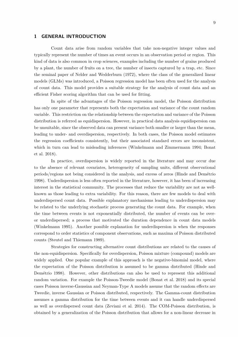
1 GENERAL INTRODUCTION
Count data arise from random variables that take non-negative integer values andtypically represent the number of times an event occurs in an observation period or region. Thiskind of data is also common in crop sciences, examples including the number of grains producedby a plant, the number of fruits on a tree, the number of insects captured by a trap, etc. Sincethe seminal paper of Nelder and Wedderburn (1972), where the class of the generalized linearmodels (GLMs) was introduced, a Poisson regression model has been often used for the analysisof count data. This model provides a suitable strategy for the analysis of count data and anefficient Fisher scoring algorithm that can be used for fitting.
In spite of the advantages of the Poisson regression model, the Poisson distributionhas only one parameter that represents both the expectation and variance of the count randomvariable. This restriction on the relationship between the expectation and variance of the Poissondistribution is referred as equidispersion. However, in practical data analysis equidispersion canbe unsuitable, since the observed data can present variance both smaller or larger than the mean,leading to under- and overdispersion, respectively. In both cases, the Poisson model estimatesthe regression coefficients consistently, but their associated standard errors are inconsistent,which in turn can lead to misleading inferences (Winkelmann and Zimmermann 1994; Bonatet al. 2018).
In practice, overdispersion is widely reported in the literature and may occur dueto the absence of relevant covariates, heterogeneity of sampling units, different observationalperiods/regions not being considered in the analysis, and excess of zeros (Hinde and Demétrio1998). Underdispersion is less often reported in the literature, however, it has been of increasinginterest in the statistical community. The processes that reduce the variability are not as well-known as those leading to extra variability. For this reason, there are few models to deal withunderdispersed count data. Possible explanatory mechanisms leading to underdispersion maybe related to the underlying stochastic process generating the count data. For example, whenthe time between events is not exponentially distributed, the number of events can be over-or underdispersed; a process that motivated the duration dependence in count data models(Winkelmann 1995). Another possible explanation for underdispersion is when the responsescorrespond to order statistics of component observations, such as maxima of Poisson distributedcounts (Steutel and Thiemann 1989).
Strategies for constructing alternative count distributions are related to the causes ofthe non-equidispersion. Specifically for overdispersion, Poisson mixture (compound) models arewidely applied. One popular example of this approach is the negative-binomial model, wherethe expectation of the Poisson distribution is assumed to be gamma distributed (Hinde andDemétrio 1998). However, other distributions can also be used to represent this additionalrandom variation. For example the Poisson-Tweedie model (Bonat et al. 2018) and its specialcases Poisson inverse-Gaussian and Neyman-Type A models assume that the random effects areTweedie, inverse Gaussian or Poisson distributed, respectively. The Gamma-count distributionassumes a gamma distribution for the time between events and it can handle underdispersedas well as overdispersed count data (Zeviani et al. 2014). The COM-Poisson distribution, isobtained by a generalization of the Poisson distribution that allows for a non-linear decrease in
10
the ratios of successive probabilities (Shmueli et al. 2005) and can be seen as a particular caseof the weigthed Poisson distribution (Del Castillo and Pérez-Casany 1998). The discretizationprocess can also be used to derive flexible discrete distributions, such as the discrete Weibulldistribution (Nakagawa and Osaki 1975; Klakattawi, Vinciotti, and Yu 2018). Related to nega-tive binomial distribution, the generalized Poisson is obtained as a limiting form of generalizednegative binomial distribution (Consul and Jain 1973). The double exponential family and theparticular double Poisson (Efron 1986) can model equi-, under- and overdispersion in countdata, as well. A comprehensive discussion on other generalizations of the Poisson distributioncan be found in Winkelmann (2008).
The standard regression for the models from the exponential family (generalized linearmodels) and for the aforementioned models is linked to the mean (or location-related) parameter.Thereby, the variance of the response variable is completely specified by the variance function(be it known or not). However, this assumption cannot be reasonable. For example, when thereis an effect of a covariate (treatment, dose, etc.) in both expectation and dispersion of thecount random variable. Smyth (1988) shows how to include a linear predictor for the dispersionas well as for the mean in the generalized linear models. In his paper, Smyth illustrates thismethodology with continuous data. For discrete data, his proposal can be extended by usingquasi-likelihood estimation methods (Wedderburn 1974; Nelder and Pregibon 1987). Besidesthat, a full parametric approach is presented by Rigby and Stasinopoulos (2005) using theso-called generalized additive models for location, scale, and shape (GAMLSS).
The main objective of this dissertation consists of exploring novel modeling approachesfor the analysis of count data. The remainder of the text is organized as follow. In Chapter2, the motivating datasets, mostly from biological experiments, and its challenges for analysisare presented. Chapter 3 is devoted to present and study our novel reparametrization of COM-Poisson models. An overview and comparison of several flexible probability distributions forcount data are addressed in Chapter 4. In Chapter 5, we consider varying dispersion in thereparametrized COM-Poisson models where the mean and the dispersion parameters may beallowed to depend on covariates. Final considerations are given in Chapter 6.
References References
Bonat, W. H., B. Jørgensen, C. C. Kokonendji, and J. Hinde (2018). “Extended Poisson-Tweedie:properties and regression model for count data”. In: Statistical Modelling 18.1, pp. 24–49.
Consul, P. C. and G. C. Jain (1973). “A Generalization of the Poisson Distribution”. In: Tech-nometrics 15.4, pp. 791–799.
Del Castillo, J. and M. Pérez-Casany (1998). “Weighted Poisson Distributions for Overdispersionand Underdispersion Situations”. In: Annals of the Institute of Statistical Mathematics 50.3,pp. 567–585.
Efron, B. (1986). “Double Exponential Families and Their Use in Generalized Linear Regression”.In: Journal of the American Statistical Association 84.395, pp. 709–721.
Hinde, J. and C. G. B. Demétrio (1998). “Overdispersion: models and estimation”. In: Compu-tational Statistics & Data Analysis 27.2, pp. 151–170.
11
Klakattawi, H. S., V. Vinciotti, and K. Yu (2018). “A Simple and Adaptive Dispersion RegressionModel for Count Data”. In: Entropy 20.142.
Nakagawa, T. and S. Osaki (1975). “The Discrete Weibull Distribution”. In: IEEE Transactionson Reliability 24.5, pp. 300–301.
Nelder, J. A. and D. Pregibon (1987). “An Extended Quasi-likelihood Function”. In: Biometrika74.2, pp. 221–232.
Nelder, J. A. and R. W. M. Wedderburn (1972). “Generalized Linear Models”. In: Journal ofthe Royal Statistical Society. Series A (General) 135, pp. 370–384.
Rigby, R. A. and D. M. Stasinopoulos (2005). “Generalized additive models for location, scaleand shape (with discussion)”. In: Journal of the Royal Statistical Society. Series C (AppliedStatistics) 54.3, pp. 507–554.
Shmueli, G., T. P. Minka, J. B. Kadane, S. Borle, and P. Boatwright (2005). “A useful dis-tribution for fitting discrete data: Revival of the Conway-Maxwell-Poisson distribution”. In:Journal of the Royal Statistical Society. Series C (Applied Statistics) 54.1, pp. 127–142.
Smyth, G. K. (1988). “Generalized Linear Models with Varying Dispersion”. In: Journal of theRoyal Statistical Society. Series B (Methodological) 51.1, pp. 47–60.
Steutel, F. W. and J. G. F. Thiemann (1989). “The gamma process and the Poisson distribution”.In: (Memorandum COSOR; Vol. 8924). Eindhoven: Technische Universiteit Eindhoven.
Wedderburn, R. W. M. (1974). “Quasi-Likelihood Functions, Generalized Linear Models, andthe Gauss-Newton Method”. In: Biometrika 61.3, p. 439.
Winkelmann, R. (1995). “Duration Dependence and Dispersion in Count-Data Models”. In:Journal of Business & Economic Statistics 13.4, pp. 467–474.
Winkelmann, R. (2008). Econometric Analysis of Count Data. 5th edition. Berlin, Heidelberg:Springer-Velag, p. 342.
Winkelmann, R. and K. F. Zimmermann (1994). “Count Data Models for Demographic Data”.In: Mathematical Population Studies 4.3, pp. 205–221.
Zeviani, W. M., P. J. Ribeiro Jr, W. H. Bonat, S. E. Shimakura, and J. A. Muniz (2014). “TheGamma-count distribution in the analysis of experimental underdispersed data”. In: Journalof Applied Statistics 41.12, pp. 2616–2626.

12
13
2 MOTIVATING STUDIES
In this chapter, we present a number of data sets to illustrate some scientific andstatistical issues which arise from count data. These data sets will be used throughout the textfor illustration of the proposed methodologies. All data sets are available in the packages cmpregand flexcm for the software R (R Core Team 2018).
2.1 Artificial defoliation in cotton phenology
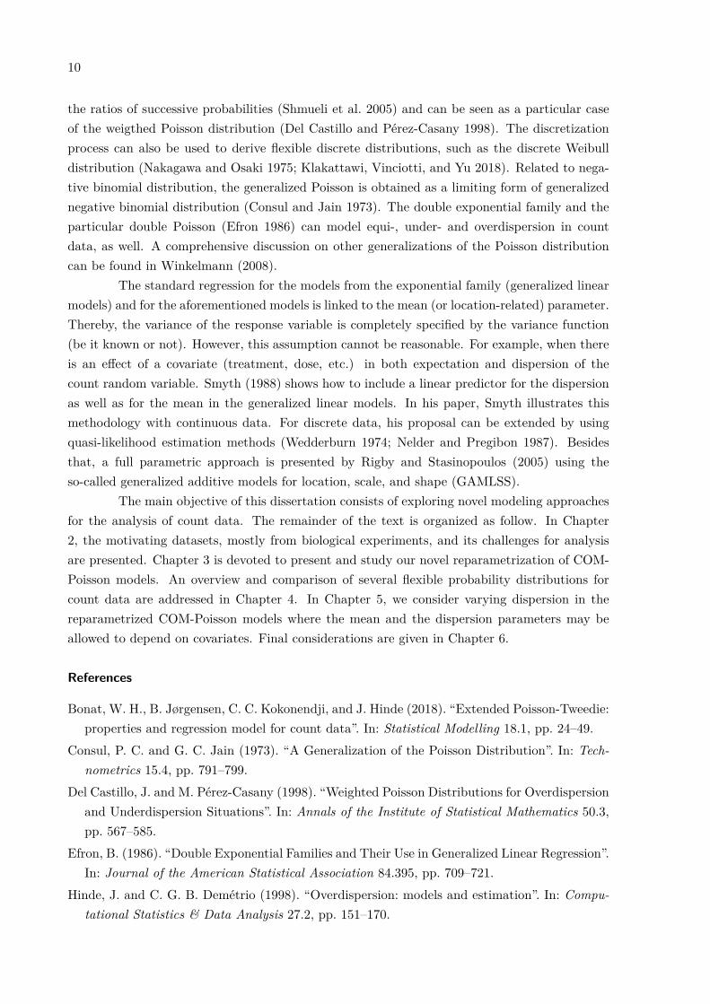
Cotton production can be drastically reduced by attack of defoliating insects. Depend-ing on the growth stage, the plants can recover from the caused damage and keep productionnot affected or can have the production reduced by low intensity defoliation. In order to studythe recovery of cotton plants (Gossypium hirsutum) in terms of production, Silva et al. (2012)conducted a greenhouse experiment under a completely randomized design with five replicates.The experimental unity was a pot with two plants and it was recorded the number of cottonbolls at five artificial defoliation levels (0%, 25%, 50%, 75%, and 100%) and five growth stages:vegetative, flower-bud, blossom, boll and boll open.
(a)Artificial defoliation level
Num
ber
of b
olls
pro
duc
ed
2
4
6
8
10
12
●●●●●
●●●●●
●●●●●
●●●●●
●●●●
●
vegetative0.00 0.25 0.50 0.75 1.00
●●●●●
●
●●●
●
●●●●●
●●●
●●
●●●●●
flower bud
●●●●
●
●●●
●●
●●●●●
●●●●●
●●●●●
blossom
0.00 0.25 0.50 0.75 1.00
●●●
●●
●●●
●●
●●●●
●
●●●●●
●●●●●
boll
2
4
6
8
10
12
●
●
●●●
●●●●
●
●●
●●●●●●
●●
●●●●●
boll open
(b)Sample mean
Sam
ple
vari
ance
0
2
4
6
8
10
0 2 4 6 8 10
●
●●
●● ●
●
●
●
●
●
●
●
●
●
●●
●
●●
●
●
● ●●
Figure 2.1. (a) Number of bolls produced for each artificial defoliation level and each growthstage (solid lines represent loess curves) and (b) sample variance against the sample mean ofthe five replicates for each combination of defoliation level and growth stage (dotted line is theidentity line and solid line is the least square line).
Figure 2.1(a) shows the number of cotton bolls recorded for each combination of de-foliation level and growth stage; the smoothers indicate that are different quadratic effects bygrowth stage. Figure 2.1(b) show that all sample variances are smaller than the sample means,suggesting underdispersion.
Alternatives analysis of this data have been proposed in the literature. Zeviani et al.(2014) analyzed it using the Gamma-count distribution. Bonat et al. (2018) used this data forillustrating the extended Poisson-Tweedie model. Huang (2017) and Ribeiro Jr et al. (2018)analyzed it by using different mean-parametrizations of the COM-Poisson model.
14
2.2 Soil moisture and potassium fertilization on soybean culture
In this second example we consider a study of potassium doses and soil moisture levelson soybean (Glicine Max) production. The tropical soils are usually poor in potassium (K)and demand potassium fertilization to obtain satisfactory yields when cultivated soybean. Fur-thermore, soybean production is affected by long exposition to water deficit. As potassium isa nutrient involved in the water balance in plant, by hyphotesis, a good supply of potassiumavoids to reduce production.
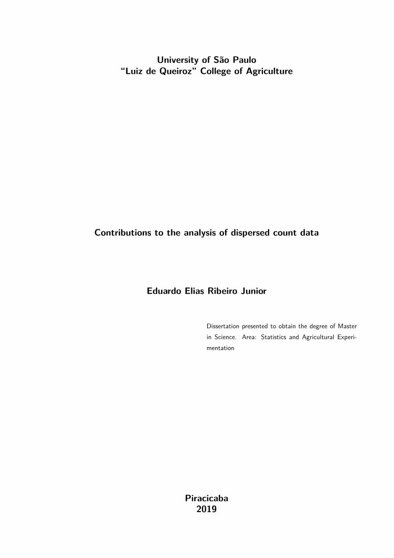
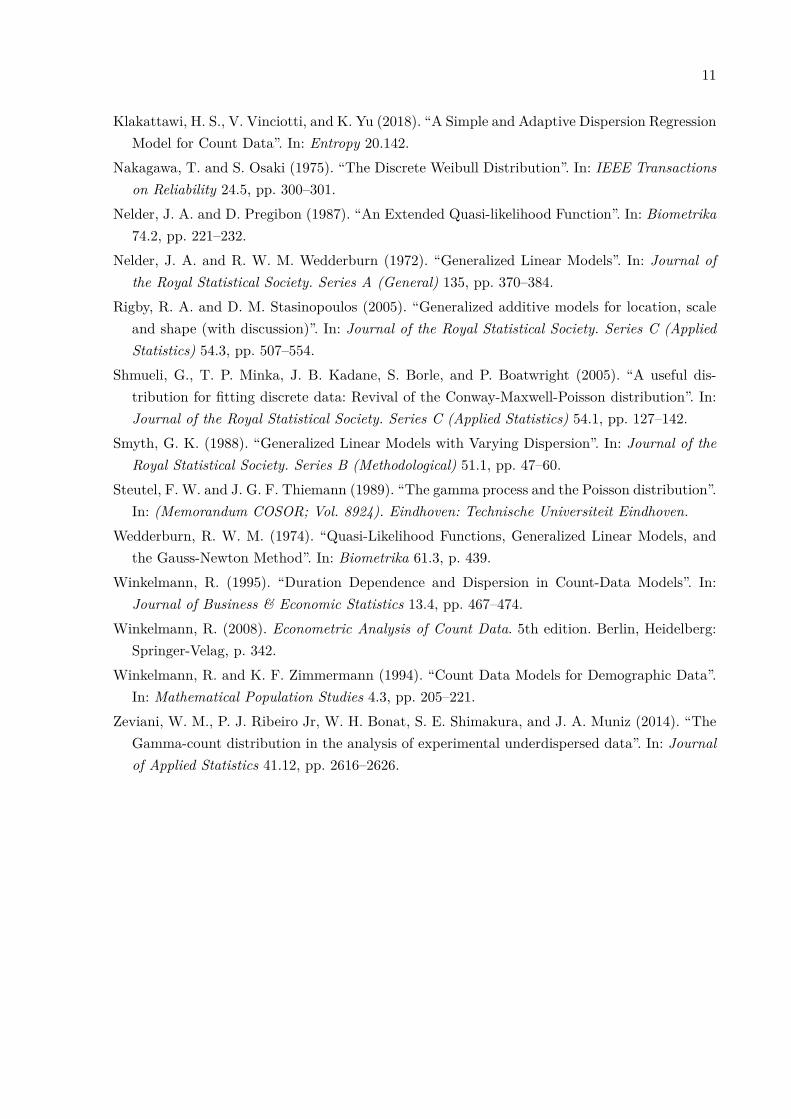
To evaluate the effects of potassium doses and soil humidity levels on soybean produc-tion, Serafim et al. (2012) conducted a 5 × 3 factorial experiment in a randomized completeblock design with 5 replicates. Five different potassium doses (0, 0.3, 0.6, 1.2 and 1.8 × 100mgdm−3) were applied to the soil and soil moisture levels were controlled at (37.5, 50, and 62.5%).The experiment was carried out in a greenhouse and the experimental units were pots with twoplants in each. The count responses measured were the total number of bean seeds per pot andthe number of pods.
(a)Potassium fertilization level
Cou
nt
50
100
150
200
250
●
● ●●
●
●
●●
●●
●
●
●
●
●
●
●
●
●
●
●
● ●
●
●
Soil moisture: 37.5%0 30 60 120 180
●
●●
●
●
●
●●
●
●
●
●●
●
●
●●
●
●
●
●
●
●
●
●
Soil moisture: 50%
0 30 60 120 180
50
100
150
200
250
●
●
●
●●
●
●
● ●●
●
●
● ●●
●●
●
●●
● ●
●●
Soil moisture: 62.5%
● Number of bean seedsNumber of pods
(b)Sample mean
Sam
ple
vari
ance
050
010
0015
00
0 500 1000 1500
●
●●
●
●
●
●
●
●
●
●
●●
●
●
Number of bean seeds
010
020
030
0
0 100 200 300
Number of pods
Figure 2.2. (a) Number of bean seeds and number of pods produced for each moisture leveland each potassium dose (solid lines represent loess curves) and (b) sample variance against thesample mean of the five replicates for each combination of moisture level and potassium dose(dotted line is the identity line and solid line is the least-squares line).
Figure 2.2(a) shows the number of bean seeds and the number of pods recorded foreach combination of potassium dose and moisture level; it is important to note the indicationof a quadratic effect of the potassium levels for both counts, as indicated by the smoothers. Forthe number of bean seeds, most points in Figure 2.2(b) are above the identity line, suggestingoverdispersion (block effect not yet removed). However, for the number of pods, there arepoints above and below the identity line – that leads to least-squares line very similar to theidentity line, suggesting that the equidispersion assumption can be suitable, if the experimentalconditions are not related to the dispersion.

15
2.3 Toxicity of nitrofen in aquatic systems
Nitrofen is a herbicide that was used extensively for the control of broad-leaved andgrass weeds in cereals and rice. Although it is relatively non-toxic to adult mammals, nitrofenis a significant teratogen and mutagen. It is also acutely toxic and reproductively toxic tocladoceran zooplankton. Nitrofen is no longer in commercial use in the United States, havingbeen the first pesticide to be withdrawn due to tetragenic effects (Bailer and Oris 1994).
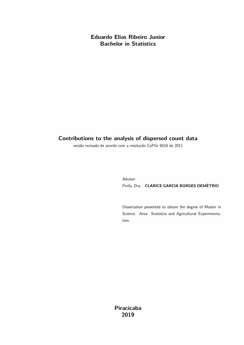
This data set comes from an experiment to measure the reproductive toxicity of theherbicide, nitrofen, on a species of zooplankton (Ceriodaphnia dubia). Fifty animals were ran-domized into batches of ten and each batch was put in a solution with a measured concentrationof nitrofen (0, 0.8, 1.6, 2.35 and 3.10 µg/100litre) (dose). Subsequently, the number of live off-spring was recorded.
Table 2.1. Sample means, sample variances and sample dispersion indexes of the ten replicatesfor each concentration level in the nitrofen study (DI = x̄/s2).
Dose N. obs. Sample mean Sample variance Sample DI0.00 10 32.40 13.1556 0.40600.80 10 31.50 10.7222 0.34041.60 10 28.30 5.5667 0.19672.35 10 17.20 34.8444 2.02583.10 10 6.00 13.7778 2.2963
Table 2.1 shows the sample mean, sample variance and sample dispersion index of thenumber of live offspring obtained from the batches with different nitrofen concentration level.This descriptive analysis indicates the nitrofen reduce the number of live offsprings howeverit seems like the dispersion is also influenced by the nitrofen concentration level (doses up to1.6µg/102litre suggesting underdispersion while doses between 1.6 and 3.1µg/102litre suggestingoverdispersion). The Figure 2.3 shows a graphical representation of these results.
(a)Nitrofen concentration level
Num
ber
of li
ve o
ffsp
ring
0
10
20
30
0.00 0.80 1.60 2.35 3.10
●
●
●●
●
●●
●
●
●
●●
●
●
●
●●
●●
● ● ●
●
●
●●●
●
●●
●
●
●
●
●
●
●
●
●
●
●●●
●
●
●●
●
●●
(b)Sample mean
Sam
ple
vari
ance
5
10
15
20
25
30
35
5 10 15 20 25 30 35
●
●
●
●
● (0.00)(0.80)
(1.60)
(2.35)
(3.10)
Figure 2.3. (a) Number of live offsprings observed for each nitrofen concentration level and(b) scatterplot of the sample means against sample variances (dotted line is the identity lineand solid line is the least-squares line).

16
2.4 Annona mucosa in control of stored maize peast
New control methods are necessary for stored grain pest management programs due toboth the widespread problems of insecticide-resistance populations and the increasing concernsof consumers regarding pesticide residues in food products. Ribeiro et al. (2013) carried outan experiment to assess the bioactivity of extracts of Annona mucosa (Annonaceae) for controlSitophilus zeamaus (Coleoptera: Curculionidae), a major pest of stored maize in Brazil. Petridishes containing 10g of corn were treated with extracts prepared with different parts of Annonamucosa (seeds, leaves and branches) or just water (control) were completely randomized with 10replicates. Then 20 Sitophilus zeamaus adults were placed in each Petri dish and the numbersof emerged insects (progeny) after 60 days were recorded.
Table 2.2. Sample means, sample variances and sample dispersion indexes of the ten replicatesfor each treatment in the maize pest study (DI = x̄/s2).
Treatment N. obs. Sample mean Sample variance Sample DIControl 10 31.50 62.5000 1.9841Leaf extract 10 31.30 94.0111 3.0035Branch extract 10 29.90 88.7667 2.9688Seed extract 10 1.10 1.6556 1.5051
For all treatments, the sample variance of the number of emerged insects treatmentis greater than their respective sample average, a strong indication of overdispersion. For leafextract, the sample variance is three times higher than the mean.
This data set is presented and analysed by Ribeiro et al. (2013) and later used byDemétrio, Hinde, and Moral (2014) for illustrating the quasi-Poisson approach for modellingoverdispersed count data.
2.5 Alternative substrats for bromeliad production
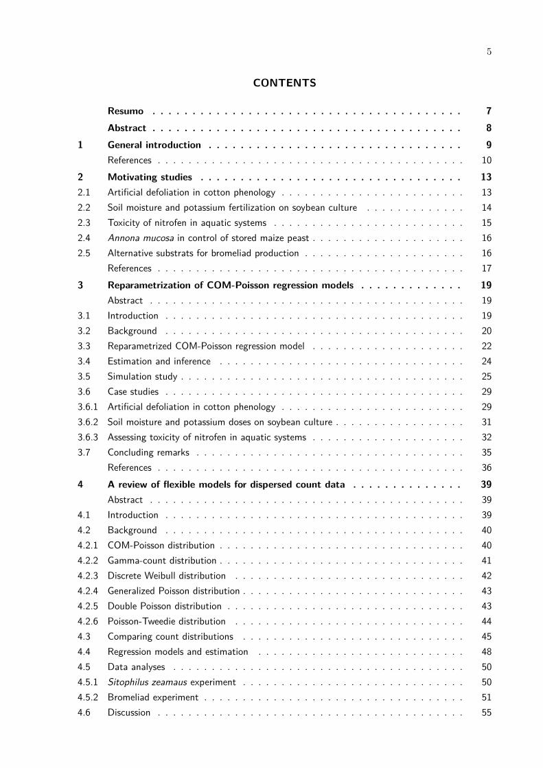
Xaxim is a substrate used in the cultivation of bromeliads and orchids, whose commer-cialization was prohibited in 2001. Since then, there has been researching in botany to proposealternative substrates to Xaxim in the cultivation of bromeliads, orchids, and other epiphytes(Salvador 2008). This dataset comes from a randomized experiment conducted in a greenhousein four blocks design with objective of evaluate five different recipients of alternative substratesfor bromeliads (Kanashiro et al. 2008). All treatments contained peat and perlite and are dif-fered in the third component: Pinus bark, Eucalyptus bark, Coxim, coconut fiber and Xaxim.The variable of interest was the number of leaves per experimental unit (pot with initially eightplants), which was registered at 4, 173, 229, 285, 341, and 435 days after planting.
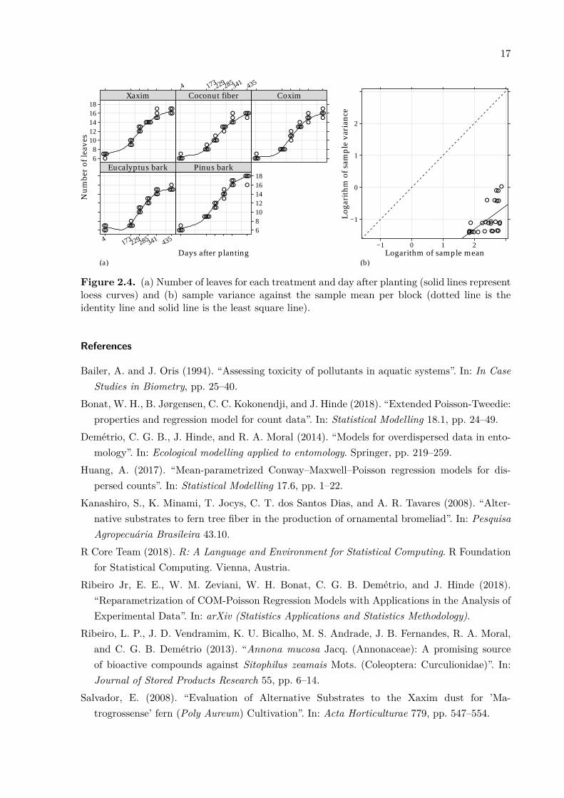
The observed number of leaves per each combination of days after planting and treat-ments are shown in Figure 2.4(a). There is a clear nonlinear (sigmoidal) relationship betweencounts and days, mainly due to the low number of leaves observed at 4 days (as expected).Figure 2.4(b) shows the sample mean and sample variances per block on the logarithm scale.All sample variances are much smaller than their sample means, even on the logarithm scale,indicating a strong evidence of underdispersion.
17
(a)Days after planting
Num
ber
of le
aves
68
1012141618
●●●●
●●●●
●●●●
●●●●●●●●
●●●●
Xaxim4 173229285341 435
●●●●
●●●●
●●●●
●●●●
●●●●
●●●●
Coconut fiber
●●●●
●●●●
●●●●
●●●● ●
●●●
●●●●
Coxim
4 173229285341 435●●●● ●●●
●
●●●●
●●●●
●●●● ●●●
●
Eucalyptus bark
681012141618
●●●●
●●●●
●●●●
●●●●
●●●●
●
●●●
Pinus bark
(b)Logarithm of sample mean
Log
arit
hm o
f sam
ple
vari
ance
−1
0
1
2
−1 0 1 2
●
● ●
●
●
● ● ● ●
●
●●
●
●
●●
●
●
● ● ●
●●
●
●
●
●
Figure 2.4. (a) Number of leaves for each treatment and day after planting (solid lines representloess curves) and (b) sample variance against the sample mean per block (dotted line is theidentity line and solid line is the least square line).
References References
Bailer, A. and J. Oris (1994). “Assessing toxicity of pollutants in aquatic systems”. In: In CaseStudies in Biometry, pp. 25–40.
Bonat, W. H., B. Jørgensen, C. C. Kokonendji, and J. Hinde (2018). “Extended Poisson-Tweedie:properties and regression model for count data”. In: Statistical Modelling 18.1, pp. 24–49.
Demétrio, C. G. B., J. Hinde, and R. A. Moral (2014). “Models for overdispersed data in ento-mology”. In: Ecological modelling applied to entomology. Springer, pp. 219–259.
Huang, A. (2017). “Mean-parametrized Conway–Maxwell–Poisson regression models for dis-persed counts”. In: Statistical Modelling 17.6, pp. 1–22.
Kanashiro, S., K. Minami, T. Jocys, C. T. dos Santos Dias, and A. R. Tavares (2008). “Alter-native substrates to fern tree fiber in the production of ornamental bromeliad”. In: PesquisaAgropecuária Brasileira 43.10.
R Core Team (2018). R: A Language and Environment for Statistical Computing. R Foundationfor Statistical Computing. Vienna, Austria.
Ribeiro Jr, E. E., W. M. Zeviani, W. H. Bonat, C. G. B. Demétrio, and J. Hinde (2018).“Reparametrization of COM-Poisson Regression Models with Applications in the Analysis ofExperimental Data”. In: arXiv (Statistics Applications and Statistics Methodology).
Ribeiro, L. P., J. D. Vendramim, K. U. Bicalho, M. S. Andrade, J. B. Fernandes, R. A. Moral,and C. G. B. Demétrio (2013). “Annona mucosa Jacq. (Annonaceae): A promising sourceof bioactive compounds against Sitophilus zeamais Mots. (Coleoptera: Curculionidae)”. In:Journal of Stored Products Research 55, pp. 6–14.
Salvador, E. (2008). “Evaluation of Alternative Substrates to the Xaxim dust for ’Ma-trogrossense’ fern (Poly Aureum) Cultivation”. In: Acta Horticulturae 779, pp. 547–554.

18
Serafim, M. E., F. B. Ono, W. M. Zeviani, J. O. Novelino, and J. V. Silva (2012). “Umidade dosolo e doses de potássio na cultura da soja”. In: Revista Ciência Agronômica 43.2, pp. 222–227.
Silva, A. M., P. E. Degrande, R. Suekane, M. G. Fernandes, and W. M. Zeviani (2012). “Impactode diferentes nı́veis de desfolha artificial nos estágios fenológicos do algodoeiro”. In: Revistade Ciências Agrárias 35.1, pp. 163–172.
Zeviani, W. M., P. J. Ribeiro Jr, W. H. Bonat, S. E. Shimakura, and J. A. Muniz (2014). “TheGamma-count distribution in the analysis of experimental underdispersed data”. In: Journalof Applied Statistics 41.12, pp. 2616–2626.
19
3 REPARAMETRIZATION OF COM-POISSON REGRESSION MODELS
ABSTRACT
The COM-Poisson distribution is a two-parameter generalization of the Poisson distributionthat can deal with under-, equi- and overdispersed count data. Unfortunately, its locationparameter does not correspond to the expectation, which complicates the parameter interpre-tation. In this paper, we propose a straightforward reparametrization of the COM-Poissondistribution based on an approximation to the expectation. Estimation and inference aredone using the likelihood paradigm. Simulation studies show that the maximum likelihoodestimators are unbiased and consistent for both regression and dispersion parameters. Inaddition, the nature of the deviance surfaces suggests that these parameters are also orthog-onal for most of the parameter space, which is advantageous for interpretation, inference,and computational efficiency. Study of the distribution’s properties, through a considerationof dispersion, zero-inflation, and heavy tail indexes, together with the results of data analy-ses show the flexibility over standard approaches. The computational routines for fitting theoriginal and reparameterized versions of the COM-Poisson regression model and data setsare available in appendix.
Keywords: COM-Poisson, Count data, Likelihood inference, Overdispersion, Underdisper-sion.
3.1 Introduction
The COM-Poisson distribution is a two-parameter generalization of the Poisson dis-tribution that includes the Poisson and geometric distributions as special cases, as well as theBernoulli distribution as a limiting case. It can deal with both under- and overdispersed countdata. Some recent applications of the COM-Poisson distribution include Lord, Geedipally, andGuikema (2010) for the analysis of traffic crash data, Sellers and Shmueli (2010) for the mod-elling of airfreight breakage and book purchases, Huang (2017) on the analysis of attendancedata, takeover bids and cotton boll counts, and Chatla and Shmueli (2018) to model counts frombike sharing systems. Theoretical results and approximations derived for this distribution arediscussed by Shmueli et al. (2005), Daly and Gaunt (2016), and Gaunt et al. (2017). The maindisadvantage of the COM-Poisson regression model as presented in Sellers and Shmueli (2010)is that its location parameter does not correspond to the expectation of the distribution. Thiscomplicates the interpretation of regression models and means that they are not comparablewith standard approaches, such as the Poisson and negative binomial regression models. Inorder to avoid this issue, Huang (2017) proposed a mean-parametrization of the COM-Poissondistribution. In his approach the mean parameter is obtained as the solution of a non-linearequation defined as an infinite sum, which is computationally demanding and liable to numericalproblems.
The main goal of this chapter is to propose a novel COM-Poisson parametrization basedon the mean approximation presented by Shmueli et al. (2005). In this parametrization, theprobability mass function is written in terms of µ and ϕ, where µ is the approximate expectationand ϕ is a dispersion parameter. In contrast to the original parametrization, the proposed
20
parametrization leads to regression coefficients directly associated (approximately) with theexpectation of the response variable, as is usual in the context of generalized linear models.Consequently, the resulting regression coefficients are comparable to those obtained by standardapproaches, such as the Poisson and negative binomial regression models. Furthermore, ournovel COM-Poisson parametrization is computationally simpler than the strategy proposed byHuang (2017), since it does not require any numerical method for solving non-linear equations.Also, we show that attractive properties like the orthogonality (Ross 1970; Cox and Reid 1987)between dispersion and regression parameters and consistency and asymptotic normality of themaximum likelihood estimators are retained.
This chapter is organized as follows. In Section 3.2 we present the COM-Poisson dis-tribution and the approach proposed by Huang (2017). The newly proposed reparametrizationis considered in Section 3.3, along with assessment of the moment approximation, and a studyof distribution’s properties. In Section 3.4 we present estimation and inference for the novelCOM-Poisson regression model in a likelihood framework. The properties of the maximumlikelihood estimators and their approximate orthogonality are assessed in Section 3.5 throughsimulation studies. We illustrate the application of the new COM-Poisson regression modelwith the analysis of three data sets. We provide an R implementation for the COM-Poisson andreparameterized COM-Poisson regression models, together with the analyzed data sets, in theappendix and online material1.
3.2 Background
The COM-Poisson distribution generalizes the Poisson distribution in terms of the ratiobetween the probabilities of two consecutive events by adding an extra dispersion parameter(Sellers and Shmueli 2010). Let Y be a COM-Poisson random variable, then
Pr(Y = y − 1)Pr(Y = y)
= yν
λ
while for the Poisson distribution this ratio is y/λ corresponding to ν = 1. This allows theCOM-Poisson distribution to deal with non-equidispersed count data. The probability massfunction of the COM-Poisson distribution is given by
Pr(Y = y | λ, ν) = λy
(y!)νZ(λ, ν), y = 0, 1, 2, . . . , (3.1)
where λ > 0, ν ≥ 0 and Z(λ, ν) =∑∞
j=0 λj/(j!)ν is a normalizing constant that depends on both
parameters.The Z(λ, ν) series diverges theoretically only when ν = 0 and λ ≥ 1, but numerically,
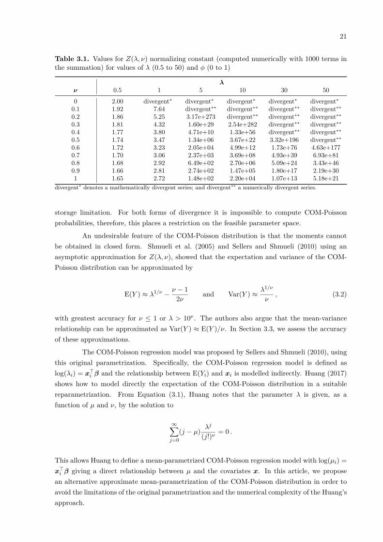
for small values of ν combined with large values of λ, the sum is so huge it results in overflow.Table 3.1 shows the values of the normalizing constant based on one thousand terms in thesummation, that is ∑1000
j=0 λj/(j!)ν , for different values of λ and ϕ.
In the first line of Table 3.1, we have mathematically divergent series, because∑∞j=0 λ
j isdivergent when λ ≥ 1. In other cases the series diverges numerically, due to the computational
1Available on http://www.leg.ufpr.br/~eduardojr/papercompanions
21
Table 3.1. Values for Z(λ, ν) normalizing constant (computed numerically with 1000 terms inthe summation) for values of λ (0.5 to 50) and ϕ (0 to 1)
λν 0.5 1 5 10 30 500 2.00 divergent∗ divergent∗ divergent∗ divergent∗ divergent∗
0.1 1.92 7.64 divergent∗∗ divergent∗∗ divergent∗∗ divergent∗∗
0.2 1.86 5.25 3.17e+273 divergent∗∗ divergent∗∗ divergent∗∗
0.3 1.81 4.32 1.60e+29 2.54e+282 divergent∗∗ divergent∗∗
0.4 1.77 3.80 4.71e+10 1.33e+56 divergent∗∗ divergent∗∗
0.5 1.74 3.47 1.34e+06 3.67e+22 3.32e+196 divergent∗∗
0.6 1.72 3.23 2.05e+04 4.99e+12 1.73e+76 4.63e+1770.7 1.70 3.06 2.37e+03 3.69e+08 4.93e+39 6.93e+810.8 1.68 2.92 6.49e+02 2.70e+06 5.09e+24 3.43e+460.9 1.66 2.81 2.74e+02 1.47e+05 1.80e+17 2.19e+301 1.65 2.72 1.48e+02 2.20e+04 1.07e+13 5.18e+21
divergent∗ denotes a mathematically divergent series; and divergent∗∗ a numerically divergent series.
storage limitation. For both forms of divergence it is impossible to compute COM-Poissonprobabilities, therefore, this places a restriction on the feasible parameter space.
An undesirable feature of the COM-Poisson distribution is that the moments cannotbe obtained in closed form. Shmueli et al. (2005) and Sellers and Shmueli (2010) using anasymptotic approximation for Z(λ, ν), showed that the expectation and variance of the COM-Poisson distribution can be approximated by
E(Y ) ≈ λ1/ν − ν − 12ν
and Var(Y ) ≈ λ1/ν
ν, (3.2)
with greatest accuracy for ν ≤ 1 or λ > 10ν . The authors also argue that the mean-variancerelationship can be approximated as Var(Y ) ≈ E(Y )/ν. In Section 3.3, we assess the accuracyof these approximations.
The COM-Poisson regression model was proposed by Sellers and Shmueli (2010), usingthis original parametrization. Specifically, the COM-Poisson regression model is defined aslog(λi) = x⊤
i β and the relationship between E(Yi) and xi is modelled indirectly. Huang (2017)shows how to model directly the expectation of the COM-Poisson distribution in a suitablereparametrization. From Equation (3.1), Huang notes that the parameter λ is given, as afunction of µ and ν, by the solution to
∞∑j=0
(j − µ) λj
(j!)ν= 0 .
This allows Huang to define a mean-parametrized COM-Poisson regression model with log(µi) =x⊤
i β giving a direct relationship between µ and the covariates x. In this article, we proposean alternative approximate mean-parametrization of the COM-Poisson distribution in order toavoid the limitations of the original parametrization and the numerical complexity of the Huang’sapproach.
22
3.3 Reparametrized COM-Poisson regression model
The proposed reparametrization of COM-Poisson models is based on the mean approx-imation (3.2). We introduce a new parameter µ, using this approximation,
µ = hν(λ) = λ1/ν − ν − 12ν
⇒ λ = h−1ν (µ) =
(µ+ (ν − 1)
2ν
)ν
. (3.3)
The dispersion parameter is taken on the log scale for computational convenience, thus ϕ =log(ν), ϕ ∈ R. The interpretation of ϕ is the same as the ν, but simply on another scale. Forϕ < 0 and ϕ > 0 we have the over- and underdispersion, respectively. When ϕ = 0, we have thePoisson distribution as a special case.
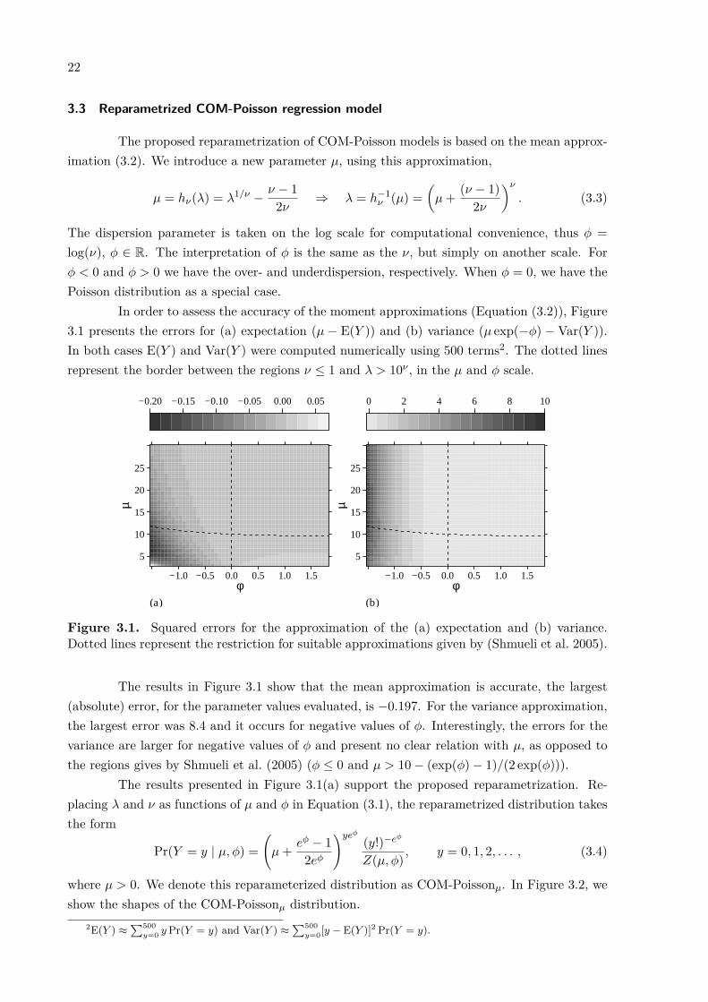
In order to assess the accuracy of the moment approximations (Equation (3.2)), Figure3.1 presents the errors for (a) expectation (µ − E(Y )) and (b) variance (µ exp(−ϕ) − Var(Y )).In both cases E(Y ) and Var(Y ) were computed numerically using 500 terms2. The dotted linesrepresent the border between the regions ν ≤ 1 and λ > 10ν , in the µ and ϕ scale.
(a)φ
µ
5
10
15
20
25
−1.0 −0.5 0.0 0.5 1.0 1.5
−0.20 −0.15 −0.10 −0.05 0.00 0.05
(b)φ
µ
5
10
15
20
25
−1.0 −0.5 0.0 0.5 1.0 1.5
0 2 4 6 8 10
Figure 3.1. Squared errors for the approximation of the (a) expectation and (b) variance.Dotted lines represent the restriction for suitable approximations given by (Shmueli et al. 2005).
The results in Figure 3.1 show that the mean approximation is accurate, the largest(absolute) error, for the parameter values evaluated, is −0.197. For the variance approximation,the largest error was 8.4 and it occurs for negative values of ϕ. Interestingly, the errors for thevariance are larger for negative values of ϕ and present no clear relation with µ, as opposed tothe regions gives by Shmueli et al. (2005) (ϕ ≤ 0 and µ > 10 − (exp(ϕ) − 1)/(2 exp(ϕ))).
The results presented in Figure 3.1(a) support the proposed reparametrization. Re-placing λ and ν as functions of µ and ϕ in Equation (3.1), the reparametrized distribution takesthe form
Pr(Y = y | µ, ϕ) =(µ+ eϕ − 1
2eϕ
)yeϕ
(y!)−eϕ
Z(µ, ϕ), y = 0, 1, 2, . . . , (3.4)
where µ > 0. We denote this reparameterized distribution as COM-Poissonµ. In Figure 3.2, weshow the shapes of the COM-Poissonµ distribution.
2E(Y ) ≈∑500
y=0 y Pr(Y = y) and Var(Y ) ≈∑500
y=0[y − E(Y )]2 Pr(Y = y).

23
y
P(Y
=y)
0.0
0.1
0.2
0.3
5 10 15 20 25
µ = 2
5 10 15 20 25
µ = 8
5 10 15 20 25
µ = 15
φ = −0.7 φ = 0.0 φ = 0.7
Figure 3.2. Shapes of the COM-Poisson distribution for different parameter values.
The constraint µ > 0 imposes an undesirable restriction in the original parameterspace, λν > (ν − 1)/(2ν). However, this restricted region is related to small underdispersedcounts (averages smaller than 0.1 and ν > 1) a parameter region unlikely to be of interest inpractice.
In order to explore the flexibility of the COM-Poisson model to deal with real countdata, we compute indexes for dispersion (DI), zero-inflation (ZI) and heavy-tail (HT), which arerespectively given by
DI = Var(Y )E(Y )
, ZI = 1 + log Pr(Y = 0)E(Y )
and HT = Pr(Y = y + 1)Pr(Y = y)
for y → ∞.
These indexes are defined in relation to the Poisson distribution. Thus, the dispersion indexindicates overdispersion for DI > 1, underdispersion for DI < 1 and equidispersion for DI = 1.The zero-inflation index indicates zero-inflation for ZI > 0, zero-deflation for ZI < 0 and noexcess of zeros for ZI = 0. Finally, the heavy-tail index indicates a heavy-tail distribution forHT → 1 when y → ∞. These indexes are discussed by Bonat et al. (2018) to study the flexibilityof Poisson-Tweedie distribution, and Puig and Valero (2006) to describe count distributions ingeneral.
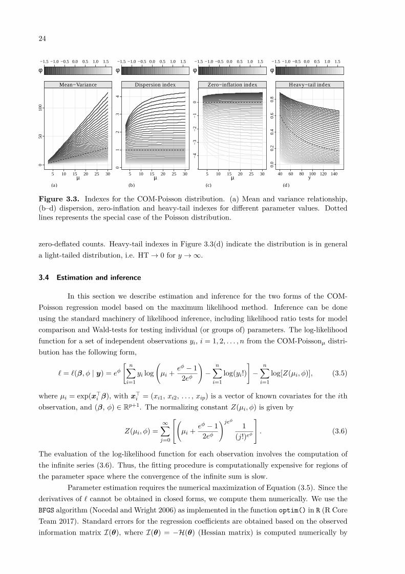
Regarding the COM-Poissonµ distribution, in Figure 3.3 we present the relationshipbetween (a) mean and variance, (b–c) the dispersion and zero-inflation indexes for differentvalues of µ and ϕ, and (d) the heavy-tail index for µ = 25 and different values of y andϕ. Figure 3.3 shows that the indexes are slightly dependent on the expected values and tendto stabilize for large values of µ. Consequently, the mean and variance relationship Figure3.3(a) is proportional to the dispersion parameter ϕ. In terms of moments, this leads to aspecification indistinguishable from the quasi-Poisson regression model. The dispersion indexesin Figure 3.3(b) show that the distribution is suitable to deal to dispersed counts, of course. Forthe parameter values evaluated the largest DI was 4.21 and smallest was 0.168. Figure 3.3(c)shows the COM-Poisson can handle a limited amount of zero-inflation, in cases of overdispersion(ϕ < 0). On the other hand, for ϕ > 0 (underdispersion) this distribution is suitable to deal with
24
(a)µ
050
100
5 10 15 20 25 30
Mean−Variance
−1.5 −1.0 −0.5 0.0 0.5 1.0 1.5
φ
(b)µ
01
23
4
5 10 15 20 25 30
Dispersion index
−1.5 −1.0 −0.5 0.0 0.5 1.0 1.5
φ
(c)µ
−4
−3
−2
−1
0
5 10 15 20 25 30
Zero−inflation index
−1.5 −1.0 −0.5 0.0 0.5 1.0 1.5
φ
(d)
y
0.0
0.2
0.4
0.6
0.8
40 60 80 100 120 140
Heavy−tail index
−1.5 −1.0 −0.5 0.0 0.5 1.0 1.5
φ
Figure 3.3. Indexes for the COM-Poisson distribution. (a) Mean and variance relationship,(b–d) dispersion, zero-inflation and heavy-tail indexes for different parameter values. Dottedlines represents the special case of the Poisson distribution.
zero-deflated counts. Heavy-tail indexes in Figure 3.3(d) indicate the distribution is in generala light-tailed distribution, i.e. HT → 0 for y → ∞.
3.4 Estimation and inference
In this section we describe estimation and inference for the two forms of the COM-Poisson regression model based on the maximum likelihood method. Inference can be doneusing the standard machinery of likelihood inference, including likelihood ratio tests for modelcomparison and Wald-tests for testing individual (or groups of) parameters. The log-likelihoodfunction for a set of independent observations yi, i = 1, 2, . . . , n from the COM-Poissonµ distri-bution has the following form,
ℓ = ℓ(β, ϕ | y) = eϕ
[n∑
i=1yi log
(µi + eϕ − 1
2eϕ
)−
n∑i=1
log(yi!)]
−n∑
i=1log[Z(µi, ϕ)], (3.5)
where µi = exp(x⊤i β), with x⊤
i = (xi1, xi2, . . . , xip) is a vector of known covariates for the ithobservation, and (β, ϕ) ∈ Rp+1. The normalizing constant Z(µi, ϕ) is given by
Z(µi, ϕ) =∞∑
j=0
(µi + eϕ − 12eϕ
)jeϕ
1(j!)eϕ
. (3.6)
The evaluation of the log-likelihood function for each observation involves the computation ofthe infinite series (3.6). Thus, the fitting procedure is computationally expensive for regions ofthe parameter space where the convergence of the infinite sum is slow.
Parameter estimation requires the numerical maximization of Equation (3.5). Since thederivatives of ℓ cannot be obtained in closed forms, we compute them numerically. We use theBFGS algorithm (Nocedal and Wright 2006) as implemented in the function optim() in R (R CoreTeam 2017). Standard errors for the regression coefficients are obtained based on the observedinformation matrix I(θ), where I(θ) = −H(θ) (Hessian matrix) is computed numerically by
25
central finite differences. Standard errors for η̂i = log(µ̂i) and hence confidence intervals areobtained by using the delta method (Pawitan 2001, p.89).
In the original parametrization, parameter estimation is analogous to that presentedfor the COM-Poissonµ distribution, however, it uses (3.5) re-expressed in terms of λ. Here, evenfor the standard COM-Poisson distribution, the dispersion parameter is taken on the log scaleto avoid numerical issues.
For the applications we also fitted the quasi-Poisson model (Wedderburn 1974) asa baseline model. This approach is based only on a second-moment assumption and withoutspecific underlying probablity model is less restrictive. In this model the variance of the responsevariable is specified by an additional dispersion parameter σ, with Var(Yi) = σµi. These modelsare fitted in R using the function glm(..., family = quasipoisson).
3.5 Simulation study
In this section, we report a simulation study to assess the properties of the maximumlikelihood estimators, the approximate parameter orthogonality of the reparametrized model,as well as the flexibility of the COM-Poisson regression model to deal with non-equidispersedcount data.
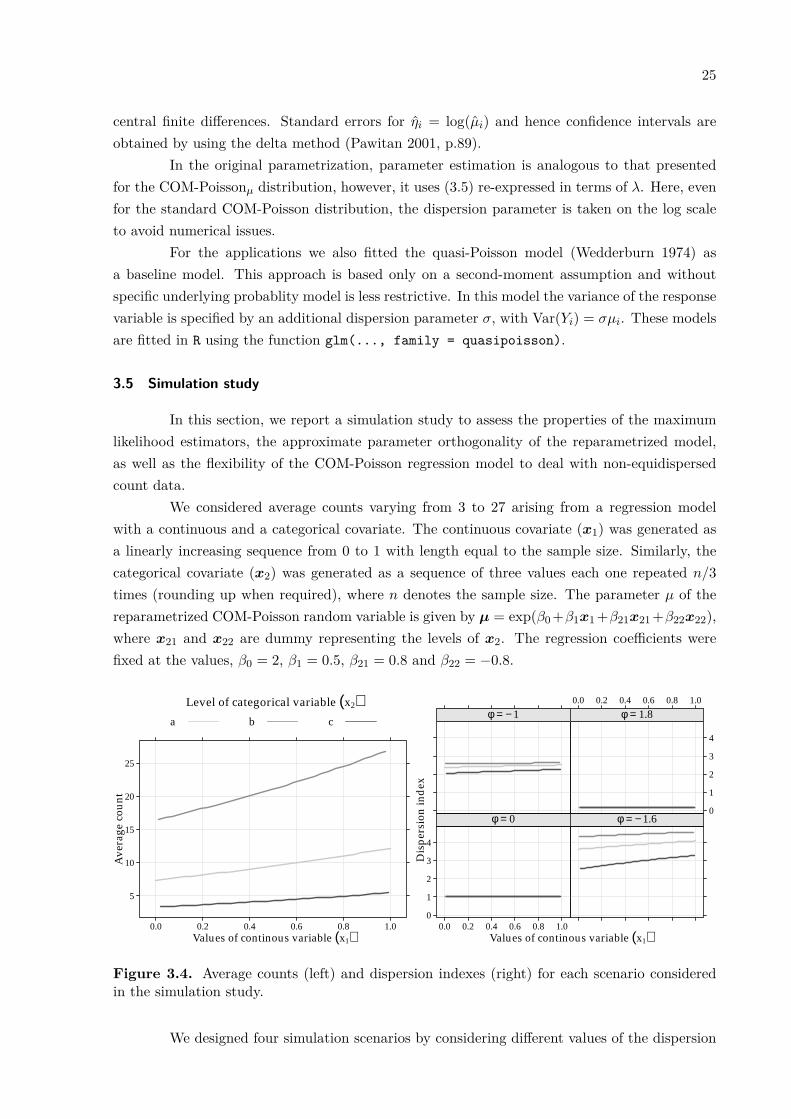
We considered average counts varying from 3 to 27 arising from a regression modelwith a continuous and a categorical covariate. The continuous covariate (x1) was generated asa linearly increasing sequence from 0 to 1 with length equal to the sample size. Similarly, thecategorical covariate (x2) was generated as a sequence of three values each one repeated n/3times (rounding up when required), where n denotes the sample size. The parameter µ of thereparametrized COM-Poisson random variable is given by µ = exp(β0 +β1x1 +β21x21 +β22x22),where x21 and x22 are dummy representing the levels of x2. The regression coefficients werefixed at the values, β0 = 2, β1 = 0.5, β21 = 0.8 and β22 = −0.8.
Values of continous variable (x1)
Ave
rage
cou
nt
5
10
15
20
25
0.0 0.2 0.4 0.6 0.8 1.0
Level of categorical variable (x2)a b c
Values of continous variable (x1)
Dis
pers
ion
ind
ex
0
1
2
3
4
0.0 0.2 0.4 0.6 0.8 1.0
φ = 0 φ = − 1.6
φ = − 10.0 0.2 0.4 0.6 0.8 1.0
0
1
2
3
4
φ = 1.8
Figure 3.4. Average counts (left) and dispersion indexes (right) for each scenario consideredin the simulation study.
We designed four simulation scenarios by considering different values of the dispersion

26
parameter ϕ = −1.6,−1.0, 0.0 and 1.8. Thus, we have strong and moderate overdispersion,equidispersion, and underdispersion, respectively. Figure 3.4 shows the variation of the averagecounts (left) and dispersion index (right) for each value of the dispersion parameter consideredin the simulation study. These configurations allow us to assess the properties of the maximumlikelihood estimators not only in extreme situations, such as high counts and low dispersion,and low counts and high dispersion, but also in the standard case of equidispersion.
In order to check the consistency of the estimators we considered four different samplesizes: 50, 100, 300 and 1000; generating 1000 data sets in each case. For sample sizes 50 and100, we have 29 and 8 simulations of the 1000 where the fitting algorithm did not converge.These non-convergence situations occurred for ϕ = −1.6. In Figure 3.5, we show the biasof the estimators for each simulation scenario (combination between values of the dispersionparameter and samples sizes) along with the confidence intervals calculated as average bias plusand minus 1.96 times the average standard error. The scales are standardized for each parameterby dividing the average bias by the average standard error obtained for the sample of size 50.
Standardized Bias
φ̂
β̂0
β̂1
β̂21
β̂22
−4 −2 0 2 4
●● ● ●●●●● ● ● ●●●
● ●●●●
● ●● ● ●
●●●● ●● ● ●●●●
● ● ●●●●●● ● ●●●●● ●●●
● ●● ●●●●●●●
●● ●
●● ● ●● ●
●●● ●● ●● ●
● ●●● ●●●●
●●●●●●●●● ●●●
●●● ●●
●● ●●● ●●●●● ●●●
●●●● ●●●●
● ●● ●●●
●●● ●
●●● ●●●● ●●●●
●●●● ●●●●●●●●
●● ●●●●● ●●●●
●● ●●●●●● ●
●
●
●
●
●
φ = − 1.6−4 −2 0 2 4
●● ●● ●●●● ●
● ●●● ● ●●● ●●● ●●
● ●● ●●
● ●● ●● ● ●
●●● ● ● ●
●●● ●● ●●●●
●●● ●●●● ●
●●● ●
●●●● ●● ●
●●●●●●●● ●
● ●● ●●●●● ●●
●●●
● ● ● ●
●● ●●
● ● ●●●●● ●●●
●●●
●●●● ●●●●●●
● ●●● ●●● ●●
●●● ●●●●
●●●
●
●
●
●
●
φ = − 1
−4 −2 0 2 4
●●● ●● ●●● ●
● ●●● ● ●●● ●● ●●
●● ●●● ● ●●● ●
●● ●● ●●● ●
●● ●●● ● ●●●● ●
●●●●● ● ●●●
●●● ●● ●●●
●● ●● ● ●●
●● ●● ●●●● ●
● ● ●●●●●●●●● ●
● ●●●● ●
●●●●●●
●
●● ●● ●●
●● ●●●● ●● ●
●●● ●●
●● ●●●●●●● ●
●●●●● ●●
●●● ●●●
●●● ●● ●● ●
●
●
●
●
●
φ = 0−4 −2 0 2 4
● ●●● ●●●● ● ●●●
●● ● ●●●
● ●●
● ●● ●● ●●●
●●● ●● ● ●●●
●●● ●●●
●●● ● ● ●
●●●●● ●
●●●● ●● ●●●●
● ● ●● ●●
●● ●●● ●● ●
●●●● ●●●●●
●● ●●
● ●● ●●● ●●●● ●
●●●● ●● ●●●●●● ●
●● ●●●● ●●
●●
● ●● ●●
●● ●●●● ●●●●
● ●●●●●●●● ●●●
●
●
●
●
●
φ = 1.8
Sample size● n=50 n=100 n=300 n=1000
Figure 3.5. Distributions of standardized bias (gray box-plots) and average with confidenceintervals (black segments) by different sample sizes and dispersion levels.
The results in Figure 3.5 show that for all dispersion levels, both the average bias andstandard errors tend to 0 as the sample size increases. Thus the estimators for the regressionparameters are unbiased, consistent and their empirical distributions are symmetric. For the
27
dispersion parameter, the estimator is asymptotically unbiased; in small samples the parameteris overestimated and the empirical distribution is slightly right-skewed.
Sample size
Cov
erag
e ra
te
0.85
0.90
0.95
200 400 600 800 1000
●
●
●
●●●
●
●
●
●
●●
●
● ●
●
φ̂
200 400 600 800 1000
●
●
●●
●
●●
●
●●
● ●
●
●
●
●
β̂0
200 400 600 800 1000
●●
● ●●●
●●●
●
●
●
●
●●
●
β̂1
200 400 600 800 1000
●
●●
●
●
●
●
●●
●
●
●●●
●●
β̂21
200 400 600 800 1000
●
●
●
●
●●
●
●
●
● ● ●
●
● ●
●
β̂22
φ = − 1.6 φ = − 1 φ = 0 φ = 1.8● ● ● ●
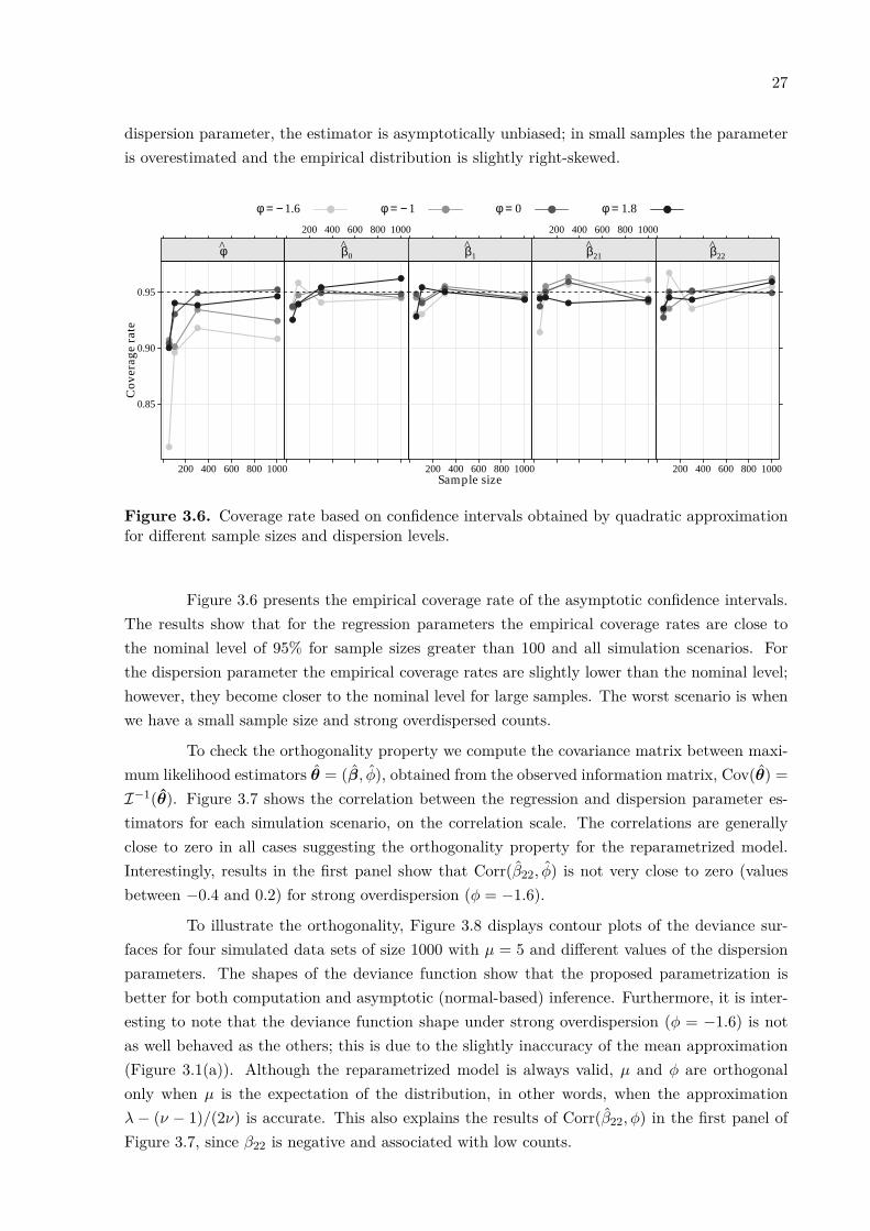
Figure 3.6. Coverage rate based on confidence intervals obtained by quadratic approximationfor different sample sizes and dispersion levels.
Figure 3.6 presents the empirical coverage rate of the asymptotic confidence intervals.The results show that for the regression parameters the empirical coverage rates are close tothe nominal level of 95% for sample sizes greater than 100 and all simulation scenarios. Forthe dispersion parameter the empirical coverage rates are slightly lower than the nominal level;however, they become closer to the nominal level for large samples. The worst scenario is whenwe have a small sample size and strong overdispersed counts.
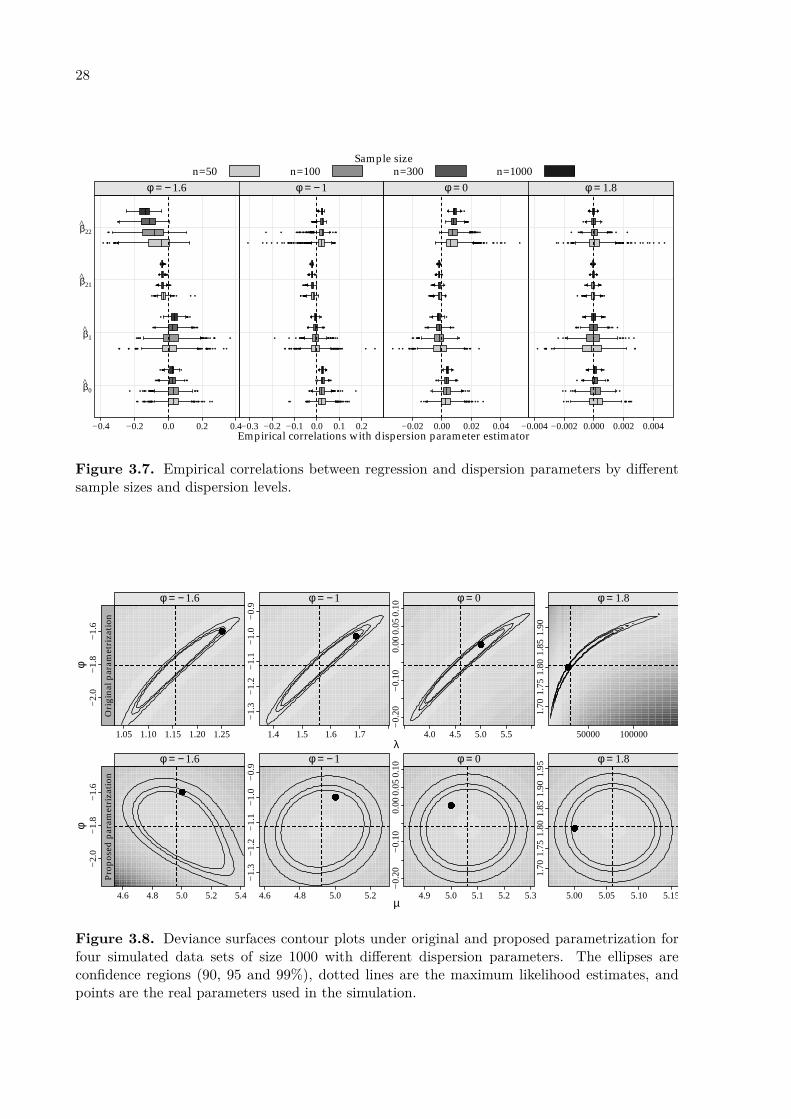
To check the orthogonality property we compute the covariance matrix between maxi-mum likelihood estimators θ̂ = (β̂, ϕ̂), obtained from the observed information matrix, Cov(θ̂) =I−1(θ̂). Figure 3.7 shows the correlation between the regression and dispersion parameter es-timators for each simulation scenario, on the correlation scale. The correlations are generallyclose to zero in all cases suggesting the orthogonality property for the reparametrized model.Interestingly, results in the first panel show that Corr(β̂22, ϕ̂) is not very close to zero (valuesbetween −0.4 and 0.2) for strong overdispersion (ϕ = −1.6).
To illustrate the orthogonality, Figure 3.8 displays contour plots of the deviance sur-faces for four simulated data sets of size 1000 with µ = 5 and different values of the dispersionparameters. The shapes of the deviance function show that the proposed parametrization isbetter for both computation and asymptotic (normal-based) inference. Furthermore, it is inter-esting to note that the deviance function shape under strong overdispersion (ϕ = −1.6) is notas well behaved as the others; this is due to the slightly inaccuracy of the mean approximation(Figure 3.1(a)). Although the reparametrized model is always valid, µ and ϕ are orthogonalonly when µ is the expectation of the distribution, in other words, when the approximationλ − (ν − 1)/(2ν) is accurate. This also explains the results of Corr(β̂22, ϕ) in the first panel ofFigure 3.7, since β22 is negative and associated with low counts.
28
Empirical correlations with dispersion parameter estimator
β̂0
β̂1
β̂21
β̂22
−0.4 −0.2 0.0 0.2 0.4
●● ●●●●● ●●● ●●● ●● ●●● ● ●● ● ●●● ●●● ●● ●●● ●● ●●
● ● ●●● ● ●● ●●● ● ●● ● ●● ●● ●●● ● ●●● ● ●● ● ● ●● ● ●
●● ● ●●●●● ●● ●● ●● ●● ●
● ● ●●●●●●● ●●●●● ●
●●● ● ●●●● ● ● ●● ●● ● ●● ●●● ● ●● ● ●●
●● ●● ●●● ●●● ●● ● ●●● ●● ●●● ●● ●
● ●● ●● ●●●● ●● ●● ●●●● ●●●● ●● ●●●●●
●●
● ●● ●●●● ●● ●
●● ●● ● ●● ●●● ● ●●
●●●●● ●●●● ● ●● ●●● ●●●● ●
●●
● ●●●●● ●●
●●●● ●● ●
●● ●●●● ●●●●●●●● ●●● ●●●●
φ = − 1.6
−0.3 −0.2 −0.1 0.0 0.1 0.2
● ● ●● ●●● ● ● ●●●● ●●● ●●● ●● ●●● ● ●●●● ●●● ●● ● ●
●● ● ●● ●●● ●●● ●●●● ● ●●● ● ●● ●●●● ●● ● ● ●● ●● ● ●●● ● ●●● ●●● ●
●●●●● ●●●●● ●●●●●●●
●●● ●● ● ●● ●● ● ●● ● ●● ● ●● ●●● ● ● ●● ● ●●● ●●● ● ●● ●● ●●●● ● ●●● ●● ● ●● ● ● ●● ●● ● ●●● ●●● ●● ● ●● ●●● ●● ●●● ● ●● ● ● ●●● ● ● ●● ●
● ●● ●● ●● ●● ●●● ● ●● ● ●●● ●● ●●●● ● ●●
●● ●●● ● ● ●●●● ●● ●● ●● ●● ●● ●●● ●●●●● ● ●●
●●● ●●●● ● ●●● ●●●
●● ●●● ●●●●● ●● ●● ●● ● ●● ● ●● ●● ●●● ●● ●● ●●● ●● ● ●● ● ●● ●●● ●●●● ●● ●● ●● ●●● ●
●●● ●●● ●●
●● ●● ●● ●
●●●●●● ●●● ●●●●
●● ●● ●● ●● ● ●●●●●● ●●●●●● ●● ● ●●● ●●●● ●● ●● ●●● ●
●●●● ●●● ●●●
● ●● ● ●
●●
●● ●●●● ●●●
φ = − 1
−0.02 0.00 0.02 0.04
● ●● ●● ●●● ●● ●● ●● ● ●● ● ●● ●●●
●● ●●● ● ●● ●● ● ●● ●● ● ●●●●●● ●●
● ●●● ●●●● ● ●●● ● ●● ●● ●● ●●●●●●●● ●●●● ● ●●
●● ●● ● ●● ● ●●● ● ●● ● ●●● ●● ● ●●● ● ●● ●●● ●●● ●●● ● ●●● ●
●● ●●● ●●● ● ●●●●
● ●●●● ●● ●● ●●
●●●● ●●●●●●● ●●●●●● ●●●● ●
● ●● ●● ● ●●● ● ●●●● ●● ●●● ●● ●● ●● ●● ●● ●●
● ●●●●● ● ●
●● ●● ● ●●●
● ●● ●●●●●●●● ●●●●
●●●●● ●●●● ●● ●● ●
●●● ●●
● ●● ●
●●●●●●●●●●●●●● ●
● ●●● ●
φ = 0
−0.004 −0.002 0.000 0.002 0.004
● ● ●●● ● ●● ● ●● ●
●● ● ●●● ●● ●●
●●● ●●● ●● ●●●● ● ●● ●● ●●●●
●●● ●● ● ●●● ● ●● ● ●● ●●● ● ●●● ● ●● ●● ●● ●● ●● ● ●● ●● ●●●● ● ●●●
●●● ●●● ● ●
● ●● ● ●● ● ●●●● ●
●●● ● ●●●●● ●● ●● ●●●
●● ●● ● ●●● ●● ● ●● ● ●●●● ●● ●●
●●● ●● ●●●● ●
● ● ●●●● ●● ●● ●● ●
● ●●● ●●●●
●●● ● ●
●●●● ●●●●●● ●● ●
●● ●● ●●● ●● ●● ● ●●● ●● ● ●● ●●
●●●● ●●●●●
●●● ●●●●●● ●● ●●●
φ = 1.8
Sample sizen=50 n=100 n=300 n=1000
Figure 3.7. Empirical correlations between regression and dispersion parameters by differentsample sizes and dispersion levels.
λ
φ−
2.0
−1.
8−
1.6
1.05 1.10 1.15 1.20 1.25
●●●●●●●●●●●●●●●●●●●●●●●●●●●●●●●●●●●●●●●●●●●●●●●●●●●●●●●●●●●●●●●●●●●●●●●●●●●●●●●●●●●●●●●●●●●●●●●●●●●●●●●●●●●●●●●●●●●●●●●●●●●●●●●●●●●●●●●●●●●●●●●●●●●●●●●●●●●●●●●●●●●●●●●●●●●●●●●●●●●●●●●●●●●●●●●●●●●●●●●●●●●●●●●●●●●●●●●●●●●●●●●●●●●●●●●●●●●●●●●●●●●●●●●●●●●●●●●●●●●●●●●●●●●●●●●●●●●●●●●●●●●●●●●●●●●●●●●●●●●●●●●●●●●●●●●●●●●●●●●●●●●●●●●●●●●●●●●●●●●●●●●●●●●●●●●●●●●●●●●●●●●●●●●●●●●●●●●●●●●●●●●●●●●●●●●●●●●●●●●●●●●●●●●●●●●●●●●●●●●●●●●●●●●●●●●●●●●●●●●●●●●●●●●●●●●●●●●●●●●●●●●●●●●●●●●●●●●●●●●●●●●●●●●●●●●●●●●●●●●●●●●●●●●●●●●●●●●●●●●●●●●●●●●●●●●●●●●●●●●●●●●●●●●●●●●●●●●●●●●●●●●●●●●●●●●●●●●●●●●●●●●●●●●●●●●●●●●●●●●●●●●●●●●●●●●●●●●●●●●●●●●●●●●●●●●●●●●●●●●●●●●●●●●●●●●●●●●●●●●●●●●●●●●●●●●●●●●●●●●●●●●●●●●●●●●●●●●●●●●●●●●●●●●●●●●●●●●●●●●●●●●●●●●●●●●●●●●●●●●●●●●●●●●●●●●●●●●●●●●●●●●●●●●●●●●●●●●●●●●●●●●●●●●●●●●●●●●●●●●●●●●●●●●●●●●●●●●●●●●●●●●●●●●●●●●●●●●●●●●●●●●●●●●●●●●●●●●●●●●●●●●●●●●●●●●●●●●●●●●●●●●●●●●●●●●●●●●●●●●●●●●●●●●●●●●●●●●●●●●●●●●●●●●●●●●●●●●●●●●●●●●●●●●●●●●●●●●●●●●●●●●●●●●●●●●●●●●●●●●●●●●●●●●●●●●●●●●●●●●●●●●●●●●●●●●●●●●●●●●●●●●●●●●●●●●●●●●●●●●●●●●●●●●●●●●●●●●●●●●●●●●●●●●●●●●●●●●●●●●●●●●●●●●●●●●●●●●●●●●●●●●●●●●●●●●●●●●●●●●●●●●●●●●●●●●●●●●●●●●●●●●●●●●●●●●●●●●●●●●●●●●●●●●●●●●●●●●●●●●●●●●●●●●●●●●●●●●●●●●●●●●●●●●●●●●●●●●●●●●●●●●●●●●●●●●●●●●●●●●●●●●●●●●●●●●●●●●●●●●●●●●●●●●●●●●●●●●●●●●●●●●●●●●●●●●●●●●●●●●●●●●●●●●●●●●●●●●●●●●●●●●●●●●●●●●●●●●●●●●●●●●●●●●●●●●●●●●●●●●●●●●●●●●●●●●●●●●●●●●●●●●●●●●●●●●●●●●●●●●●●●●●●●●●●●●●●●●●●●●●●●●●●●●●●●●●●●●●●●●●●●●●●●●●●●●●●●●●●●●●●●●●●●●●●●●●●●●●●●●●●●●●●●●●●●●●●●●●●●●●●●●●●●●●●●●●●●●●●●●●●●●●●●●●●●●●●●●●●●●●●●●●●●●●●●●●●●●●●●●●●●●●●●●●●●●●●●●●●●●●●●●●●●●●●●●●●●●●●●●●●●●●●●●●●●●●●●●●●●●●●●●●●●●●●●●●●●●●●●●●●●●●●●●●●●●●●●●●●●●●●●●●●●●●●●●●●●●●●●●●●●●●●●●●●●●●●●●●●●●●●●●●●●●●●●●●●●●●●●●●●●●●●●●●●●●●●●●●●●●●●●●●●●●●●●●●●●●●●●●●●●●●●●●●●●●●●●●●●●●●●●●●●●●●●●●●●●●●●●●●●●●●●●●●●●●●●●●●●●●●●●●●●●●●●●●●●●●●●●●●●●●●●●●●●●●●●●●●●●●●●●●●●●●●●●●●●●●●●●●●●●●●●●●●●●●●●●●●●●●●●●●●●●●●●●●●●●●●●●●●●●●●●●●●●●●●●●●●●●●●●●●●●●●●●●●●●●●●●●●●●●●●●●●●●●●●●●●●●●●●●●●●●●●●●●●●●●●●●●●●●●●●●●●●●●●●●●●●●●●●●●●●●●●●●●●●●●●●●●●●●●●●●●●●●●●●●●●●●●●●●●●●●●●●●●●●●●●●●●●●●●●●●●●●●●●●●●●●●●●●●●●●●●●●●●●●●●●●●●●●●●●●●●●●●●●●●●●●●●●●●●●●●●●●●●●●●●●●●●●●●●●●●●●●●●●●●●●●●●●●●●●●●●●●●●●●●●●●●●●●●●●●●●●●●●●●●●●●●●●●●●●●●●●●●●●●●●●●●●●●●●●●●●●●●●●●●●●●●●●●●●●●●●●●●●●●●●●●●●●●●●●●●●●●●●●●●●●●●●●●●●●●●●●●●●●●●●●●●●●●●●●●●●●●●●●●●●●●●●●●●●●●●●●●●●●●●●●●●●●●●●●●●●●●●●●●●●●●●●●●●●●●●●●●●●●●●●●●●●●●●●●●●●●●●●●●●●●●●●●●●●●●●●●●●●●●●●●●●●●●●●●●●●●●●●●●●●●●●●●●●●●●●●●●●●●●●●●●●●●●●●●●●●●●●●●●●●●●●●●●
φ = − 1.6
Ori
gina
l par
amet
riza
tion
−1.
3−
1.2
−1.
1−
1.0
−0.
9
1.4 1.5 1.6 1.7
●●●●●●●●●●●●●●●●●●●●●●●●●●●●●●●●●●●●●●●●●●●●●●●●●●●●●●●●●●●●●●●●●●●●●●●●●●●●●●●●●●●●●●●●●●●●●●●●●●●●●●●●●●●●●●●●●●●●●●●●●●●●●●●●●●●●●●●●●●●●●●●●●●●●●●●●●●●●●●●●●●●●●●●●●●●●●●●●●●●●●●●●●●●●●●●●●●●●●●●●●●●●●●●●●●●●●●●●●●●●●●●●●●●●●●●●●●●●●●●●●●●●●●●●●●●●●●●●●●●●●●●●●●●●●●●●●●●●●●●●●●●●●●●●●●●●●●●●●●●●●●●●●●●●●●●●●●●●●●●●●●●●●●●●●●●●●●●●●●●●●●●●●●●●●●●●●●●●●●●●●●●●●●●●●●●●●●●●●●●●●●●●●●●●●●●●●●●●●●●●●●●●●●●●●●●●●●●●●●●●●●●●●●●●●●●●●●●●●●●●●●●●●●●●●●●●●●●●●●●●●●●●●●●●●●●●●●●●●●●●●●●●●●●●●●●●●●●●●●●●●●●●●●●●●●●●●●●●●●●●●●●●●●●●●●●●●●●●●●●●●●●●●●●●●●●●●●●●●●●●●●●●●●●●●●●●●●●●●●●●●●●●●●●●●●●●●●●●●●●●●●●●●●●●●●●●●●●●●●●●●●●●●●●●●●●●●●●●●●●●●●●●●●●●●●●●●●●●●●●●●●●●●●●●●●●●●●●●●●●●●●●●●●●●●●●●●●●●●●●●●●●●●●●●●●●●●●●●●●●●●●●●●●●●●●●●●●●●●●●●●●●●●●●●●●●●●●●●●●●●●●●●●●●●●●●●●●●●●●●●●●●●●●●●●●●●●●●●●●●●●●●●●●●●●●●●●●●●●●●●●●●●●●●●●●●●●●●●●●●●●●●●●●●●●●●●●●●●●●●●●●●●●●●●●●●●●●●●●●●●●●●●●●●●●●●●●●●●●●●●●●●●●●●●●●●●●●●●●●●●●●●●●●●●●●●●●●●●●●●●●●●●●●●●●●●●●●●●●●●●●●●●●●●●●●●●●●●●●●●●●●●●●●●●●●●●●●●●●●●●●●●●●●●●●●●●●●●●●●●●●●●●●●●●●●●●●●●●●●●●●●●●●●●●●●●●●●●●●●●●●●●●●●●●●●●●●●●●●●●●●●●●●●●●●●●●●●●●●●●●●●●●●●●●●●●●●●●●●●●●●●●●●●●●●●●●●●●●●●●●●●●●●●●●●●●●●●●●●●●●●●●●●●●●●●●●●●●●●●●●●●●●●●●●●●●●●●●●●●●●●●●●●●●●●●●●●●●●●●●●●●●●●●●●●●●●●●●●●●●●●●●●●●●●●●●●●●●●●●●●●●●●●●●●●●●●●●●●●●●●●●●●●●●●●●●●●●●●●●●●●●●●●●●●●●●●●●●●●●●●●●●●●●●●●●●●●●●●●●●●●●●●●●●●●●●●●●●●●●●●●●●●●●●●●●●●●●●●●●●●●●●●●●●●●●●●●●●●●●●●●●●●●●●●●●●●●●●●●●●●●●●●●●●●●●●●●●●●●●●●●●●●●●●●●●●●●●●●●●●●●●●●●●●●●●●●●●●●●●●●●●●●●●●●●●●●●●●●●●●●●●●●●●●●●●●●●●●●●●●●●●●●●●●●●●●●●●●●●●●●●●●●●●●●●●●●●●●●●●●●●●●●●●●●●●●●●●●●●●●●●●●●●●●●●●●●●●●●●●●●●●●●●●●●●●●●●●●●●●●●●●●●●●●●●●●●●●●●●●●●●●●●●●●●●●●●●●●●●●●●●●●●●●●●●●●●●●●●●●●●●●●●●●●●●●●●●●●●●●●●●●●●●●●●●●●●●●●●●●●●●●●●●●●●●●●●●●●●●●●●●●●●●●●●●●●●●●●●●●●●●●●●●●●●●●●●●●●●●●●●●●●●●●●●●●●●●●●●●●●●●●●●●●●●●●●●●●●●●●●●●●●●●●●●●●●●●●●●●●●●●●●●●●●●●●●●●●●●●●●●●●●●●●●●●●●●●●●●●●●●●●●●●●●●●●●●●●●●●●●●●●●●●●●●●●●●●●●●●●●●●●●●●●●●●●●●●●●●●●●●●●●●●●●●●●●●●●●●●●●●●●●●●●●●●●●●●●●●●●●●●●●●●●●●●●●●●●●●●●●●●●●●●●●●●●●●●●●●●●●●●●●●●●●●●●●●●●●●●●●●●●●●●●●●●●●●●●●●●●●●●●●●●●●●●●●●●●●●●●●●●●●●●●●●●●●●●●●●●●●●●●●●●●●●●●●●●●●●●●●●●●●●●●●●●●●●●●●●●●●●●●●●●●●●●●●●●●●●●●●●●●●●●●●●●●●●●●●●●●●●●●●●●●●●●●●●●●●●●●●●●●●●●●●●●●●●●●●●●●●●●●●●●●●●●●●●●●●●●●●●●●●●●●●●●●●●●●●●●●●●●●●●●●●●●●●●●●●●●●●●●●●●●●●●●●●●●●●●●●●●●●●●●●●●●●●●●●●●●●●●●●●●●●●●●●●●●●●●●●●●●●●●●●●●●●●●●●●●●●●●●●●●●●●●●●●●●●●●●●●●●●●●●●●●●●●●●●●●●●●●●●●●●●●●●●●●●●●●●●●●●●●●●●●●●●●●●●●●●●●●●●●●●●●●●●●●●●●●●●●●●●●●●●●●●●●●●●●●●●●●●●●●●●●●●●●●●●●●●●●●
φ = − 1
−0.
20−
0.10
0.00
0.05
0.10
4.0 4.5 5.0 5.5
●●●●●●●●●●●●●●●●●●●●●●●●●●●●●●●●●●●●●●●●●●●●●●●●●●●●●●●●●●●●●●●●●●●●●●●●●●●●●●●●●●●●●●●●●●●●●●●●●●●●●●●●●●●●●●●●●●●●●●●●●●●●●●●●●●●●●●●●●●●●●●●●●●●●●●●●●●●●●●●●●●●●●●●●●●●●●●●●●●●●●●●●●●●●●●●●●●●●●●●●●●●●●●●●●●●●●●●●●●●●●●●●●●●●●●●●●●●●●●●●●●●●●●●●●●●●●●●●●●●●●●●●●●●●●●●●●●●●●●●●●●●●●●●●●●●●●●●●●●●●●●●●●●●●●●●●●●●●●●●●●●●●●●●●●●●●●●●●●●●●●●●●●●●●●●●●●●●●●●●●●●●●●●●●●●●●●●●●●●●●●●●●●●●●●●●●●●●●●●●●●●●●●●●●●●●●●●●●●●●●●●●●●●●●●●●●●●●●●●●●●●●●●●●●●●●●●●●●●●●●●●●●●●●●●●●●●●●●●●●●●●●●●●●●●●●●●●●●●●●●●●●●●●●●●●●●●●●●●●●●●●●●●●●●●●●●●●●●●●●●●●●●●●●●●●●●●●●●●●●●●●●●●●●●●●●●●●●●●●●●●●●●●●●●●●●●●●●●●●●●●●●●●●●●●●●●●●●●●●●●●●●●●●●●●●●●●●●●●●●●●●●●●●●●●●●●●●●●●●●●●●●●●●●●●●●●●●●●●●●●●●●●●●●●●●●●●●●●●●●●●●●●●●●●●●●●●●●●●●●●●●●●●●●●●●●●●●●●●●●●●●●●●●●●●●●●●●●●●●●●●●●●●●●●●●●●●●●●●●●●●●●●●●●●●●●●●●●●●●●●●●●●●●●●●●●●●●●●●●●●●●●●●●●●●●●●●●●●●●●●●●●●●●●●●●●●●●●●●●●●●●●●●●●●●●●●●●●●●●●●●●●●●●●●●●●●●●●●●●●●●●●●●●●●●●●●●●●●●●●●●●●●●●●●●●●●●●●●●●●●●●●●●●●●●●●●●●●●●●●●●●●●●●●●●●●●●●●●●●●●●●●●●●●●●●●●●●●●●●●●●●●●●●●●●●●●●●●●●●●●●●●●●●●●●●●●●●●●●●●●●●●●●●●●●●●●●●●●●●●●●●●●●●●●●●●●●●●●●●●●●●●●●●●●●●●●●●●●●●●●●●●●●●●●●●●●●●●●●●●●●●●●●●●●●●●●●●●●●●●●●●●●●●●●●●●●●●●●●●●●●●●●●●●●●●●●●●●●●●●●●●●●●●●●●●●●●●●●●●●●●●●●●●●●●●●●●●●●●●●●●●●●●●●●●●●●●●●●●●●●●●●●●●●●●●●●●●●●●●●●●●●●●●●●●●●●●●●●●●●●●●●●●●●●●●●●●●●●●●●●●●●●●●●●●●●●●●●●●●●●●●●●●●●●●●●●●●●●●●●●●●●●●●●●●●●●●●●●●●●●●●●●●●●●●●●●●●●●●●●●●●●●●●●●●●●●●●●●●●●●●●●●●●●●●●●●●●●●●●●●●●●●●●●●●●●●●●●●●●●●●●●●●●●●●●●●●●●●●●●●●●●●●●●●●●●●●●●●●●●●●●●●●●●●●●●●●●●●●●●●●●●●●●●●●●●●●●●●●●●●●●●●●●●●●●●●●●●●●●●●●●●●●●●●●●●●●●●●●●●●●●●●●●●●●●●●●●●●●●●●●●●●●●●●●●●●●●●●●●●●●●●●●●●●●●●●●●●●●●●●●●●●●●●●●●●●●●●●●●●●●●●●●●●●●●●●●●●●●●●●●●●●●●●●●●●●●●●●●●●●●●●●●●●●●●●●●●●●●●●●●●●●●●●●●●●●●●●●●●●●●●●●●●●●●●●●●●●●●●●●●●●●●●●●●●●●●●●●●●●●●●●●●●●●●●●●●●●●●●●●●●●●●●●●●●●●●●●●●●●●●●●●●●●●●●●●●●●●●●●●●●●●●●●●●●●●●●●●●●●●●●●●●●●●●●●●●●●●●●●●●●●●●●●●●●●●●●●●●●●●●●●●●●●●●●●●●●●●●●●●●●●●●●●●●●●●●●●●●●●●●●●●●●●●●●●●●●●●●●●●●●●●●●●●●●●●●●●●●●●●●●●●●●●●●●●●●●●●●●●●●●●●●●●●●●●●●●●●●●●●●●●●●●●●●●●●●●●●●●●●●●●●●●●●●●●●●●●●●●●●●●●●●●●●●●●●●●●●●●●●●●●●●●●●●●●●●●●●●●●●●●●●●●●●●●●●●●●●●●●●●●●●●●●●●●●●●●●●●●●●●●●●●●●●●●●●●●●●●●●●●●●●●●●●●●●●●●●●●●●●●●●●●●●●●●●●●●●●●●●●●●●●●●●●●●●●●●●●●●●●●●●●●●●●●●●●●●●●●●●●●●●●●●●●●●●●●●●●●●●●●●●●●●●●●●●●●●●●●●●●●●●●●●●●●●●●●●●●●●●●●●●●●●●●●●●●●●●●●●●●●●●●●●●●●●●●●●●●●●●●●●●●●●●●●●●●●●●●●●●●●●●●●●●●●●●●●●●●●●●●●●●●●●●●●●●●●●●●●●●●●●●●●●●●●●●●●●●●●●●●●●●●●●●●●●●●●●●●●●●●●●●●●●●●●●●●●●●●●●●●●●●●●●●●●●●●●●●●●●●●●●●●●●●●●●●●●●●●●●●●●●●●●●●●●●●●●●●●●●●●
φ = 0
1.70
1.75
1.80
1.85
1.90
50000 100000
●●●●●●●●●●●●●●●●●●●●●●●●●●●●●●●●●●●●●●●●●●●●●●●●●●●●●●●●●●●●●●●●●●●●●●●●●●●●●●●●●●●●●●●●●●●●●●●●●●●●●●●●●●●●●●●●●●●●●●●●●●●●●●●●●●●●●●●●●●●●●●●●●●●●●●●●●●●●●●●●●●●●●●●●●●●●●●●●●●●●●●●●●●●●●●●●●●●●●●●●●●●●●●●●●●●●●●●●●●●●●●●●●●●●●●●●●●●●●●●●●●●●●●●●●●●●●●●●●●●●●●●●●●●●●●●●●●●●●●●●●●●●●●●●●●●●●●●●●●●●●●●●●●●●●●●●●●●●●●●●●●●●●●●●●●●●●●●●●●●●●●●●●●●●●●●●●●●●●●●●●●●●●●●●●●●●●●●●●●●●●●●●●●●●●●●●●●●●●●●●●●●●●●●●●●●●●●●●●●●●●●●●●●●●●●●●●●●●●●●●●●●●●●●●●●●●●●●●●●●●●●●●●●●●●●●●●●●●●●●●●●●●●●●●●●●●●●●●●●●●●●●●●●●●●●●●●●●●●●●●●●●●●●●●●●●●●●●●●●●●●●●●●●●●●●●●●●●●●●●●●●●●●●●●●●●●●●●●●●●●●●●●●●●●●●●●●●●●●●●●●●●●●●●●●●●●●●●●●●●●●●●●●●●●●●●●●●●●●●●●●●●●●●●●●●●●●●●●●●●●●●●●●●●●●●●●●●●●●●●●●●●●●●●●●●●●●●●●●●●●●●●●●●●●●●●●●●●●●●●●●●●●●●●●●●●●●●●●●●●●●●●●●●●●●●●●●●●●●●●●●●●●●●●●●●●●●●●●●●●●●●●●●●●●●●●●●●●●●●●●●●●●●●●●●●●●●●●●●●●●●●●●●●●●●●●●●●●●●●●●●●●●●●●●●●●●●●●●●●●●●●●●●●●●●●●●●●●●●●●●●●●●●●●●●●●●●●●●●●●●●●●●●●●●●●●●●●●●●●●●●●●●●●●●●●●●●●●●●●●●●●●●●●●●●●●●●●●●●●●●●●●●●●●●●●●●●●●●●●●●●●●●●●●●●●●●●●●●●●●●●●●●●●●●●●●●●●●●●●●●●●●●●●●●●●●●●●●●●●●●●●●●●●●●●●●●●●●●●●●●●●●●●●●●●●●●●●●●●●●●●●●●●●●●●●●●●●●●●●●●●●●●●●●●●●●●●●●●●●●●●●●●●●●●●●●●●●●●●●●●●●●●●●●●●●●●●●●●●●●●●●●●●●●●●●●●●●●●●●●●●●●●●●●●●●●●●●●●●●●●●●●●●●●●●●●●●●●●●●●●●●●●●●●●●●●●●●●●●●●●●●●●●●●●●●●●●●●●●●●●●●●●●●●●●●●●●●●●●●●●●●●●●●●●●●●●●●●●●●●●●●●●●●●●●●●●●●●●●●●●●●●●●●●●●●●●●●●●●●●●●●●●●●●●●●●●●●●●●●●●●●●●●●●●●●●●●●●●●●●●●●●●●●●●●●●●●●●●●●●●●●●●●●●●●●●●●●●●●●●●●●●●●●●●●●●●●●●●●●●●●●●●●●●●●●●●●●●●●●●●●●●●●●●●●●●●●●●●●●●●●●●●●●●●●●●●●●●●●●●●●●●●●●●●●●●●●●●●●●●●●●●●●●●●●●●●●●●●●●●●●●●●●●●●●●●●●●●●●●●●●●●●●●●●●●●●●●●●●●●●●●●●●●●●●●●●●●●●●●●●●●●●●●●●●●●●●●●●●●●●●●●●●●●●●●●●●●●●●●●●●●●●●●●●●●●●●●●●●●●●●●●●●●●●●●●●●●●●●●●●●●●●●●●●●●●●●●●●●●●●●●●●●●●●●●●●●●●●●●●●●●●●●●●●●●●●●●●●●●●●●●●●●●●●●●●●●●●●●●●●●●●●●●●●●●●●●●●●●●●●●●●●●●●●●●●●●●●●●●●●●●●●●●●●●●●●●●●●●●●●●●●●●●●●●●●●●●●●●●●●●●●●●●●●●●●●●●●●●●●●●●●●●●●●●●●●●●●●●●●●●●●●●●●●●●●●●●●●●●●●●●●●●●●●●●●●●●●●●●●●●●●●●●●●●●●●●●●●●●●●●●●●●●●●●●●●●●●●●●●●●●●●●●●●●●●●●●●●●●●●●●●●●●●●●●●●●●●●●●●●●●●●●●●●●●●●●●●●●●●●●●●●●●●●●●●●●●●●●●●●●●●●●●●●●●●●●●●●●●●●●●●●●●●●●●●●●●●●●●●●●●●●●●●●●●●●●●●●●●●●●●●●●●●●●●●●●●●●●●●●●●●●●●●●●●●●●●●●●●●●●●●●●●●●●●●●●●●●●●●●●●●●●●●●●●●●●●●●●●●●●●●●●●●●●●●●●●●●●●●●●●●●●●●●●●●●●●●●●●●●●●●●●●●●●●●●●●●●●●●●●●●●●●●●●●●●●●●●●●●●●●●●●●●●●●●●●●●●●●●●●●●●●●●●●●●●●●●●●●●●●●●●●●●●●●●●●●●●●●●●●●●●●●●●●●●●●●●●●●●●●●●●●●●●●●●●●●●●●●●●●●●●●●●●●●●●●●●●●●●●●●●●●●●●●●●●●●●●●●●●●●●●●●●●●●●●●●●●●●●●●●●●●●●●●●●●●●●●●●●●●●●●●●●●●●●●●●●●●●●●●●●●●●●●●●●●●●●●●●●●●●●●●●●●●●●●●●●●●●●●
φ = 1.8
µ
φ−
2.0
−1.
8−
1.6
4.6 4.8 5.0 5.2 5.4
●●●●●●●●●●●●●●●●●●●●●●●●●●●●●●●●●●●●●●●●●●●●●●●●●●●●●●●●●●●●●●●●●●●●●●●●●●●●●●●●●●●●●●●●●●●●●●●●●●●●●●●●●●●●●●●●●●●●●●●●●●●●●●●●●●●●●●●●●●●●●●●●●●●●●●●●●●●●●●●●●●●●●●●●●●●●●●●●●●●●●●●●●●●●●●●●●●●●●●●●●●●●●●●●●●●●●●●●●●●●●●●●●●●●●●●●●●●●●●●●●●●●●●●●●●●●●●●●●●●●●●●●●●●●●●●●●●●●●●●●●●●●●●●●●●●●●●●●●●●●●●●●●●●●●●●●●●●●●●●●●●●●●●●●●●●●●●●●●●●●●●●●●●●●●●●●●●●●●●●●●●●●●●●●●●●●●●●●●●●●●●●●●●●●●●●●●●●●●●●●●●●●●●●●●●●●●●●●●●●●●●●●●●●●●●●●●●●●●●●●●●●●●●●●●●●●●●●●●●●●●●●●●●●●●●●●●●●●●●●●●●●●●●●●●●●●●●●●●●●●●●●●●●●●●●●●●●●●●●●●●●●●●●●●●●●●●●●●●●●●●●●●●●●●●●●●●●●●●●●●●●●●●●●●●●●●●●●●●●●●●●●●●●●●●●●●●●●●●●●●●●●●●●●●●●●●●●●●●●●●●●●●●●●●●●●●●●●●●●●●●●●●●●●●●●●●●●●●●●●●●●●●●●●●●●●●●●●●●●●●●●●●●●●●●●●●●●●●●●●●●●●●●●●●●●●●●●●●●●●●●●●●●●●●●●●●●●●●●●●●●●●●●●●●●●●●●●●●●●●●●●●●●●●●●●●●●●●●●●●●●●●●●●●●●●●●●●●●●●●●●●●●●●●●●●●●●●●●●●●●●●●●●●●●●●●●●●●●●●●●●●●●●●●●●●●●●●●●●●●●●●●●●●●●●●●●●●●●●●●●●●●●●●●●●●●●●●●●●●●●●●●●●●●●●●●●●●●●●●●●●●●●●●●●●●●●●●●●●●●●●●●●●●●●●●●●●●●●●●●●●●●●●●●●●●●●●●●●●●●●●●●●●●●●●●●●●●●●●●●●●●●●●●●●●●●●●●●●●●●●●●●●●●●●●●●●●●●●●●●●●●●●●●●●●●●●●●●●●●●●●●●●●●●●●●●●●●●●●●●●●●●●●●●●●●●●●●●●●●●●●●●●●●●●●●●●●●●●●●●●●●●●●●●●●●●●●●●●●●●●●●●●●●●●●●●●●●●●●●●●●●●●●●●●●●●●●●●●●●●●●●●●●●●●●●●●●●●●●●●●●●●●●●●●●●●●●●●●●●●●●●●●●●●●●●●●●●●●●●●●●●●●●●●●●●●●●●●●●●●●●●●●●●●●●●●●●●●●●●●●●●●●●●●●●●●●●●●●●●●●●●●●●●●●●●●●●●●●●●●●●●●●●●●●●●●●●●●●●●●●●●●●●●●●●●●●●●●●●●●●●●●●●●●●●●●●●●●●●●●●●●●●●●●●●●●●●●●●●●●●●●●●●●●●●●●●●●●●●●●●●●●●●●●●●●●●●●●●●●●●●●●●●●●●●●●●●●●●●●●●●●●●●●●●●●●●●●●●●●●●●●●●●●●●●●●●●●●●●●●●●●●●●●●●●●●●●●●●●●●●●●●●●●●●●●●●●●●●●●●●●●●●●●●●●●●●●●●●●●●●●●●●●●●●●●●●●●●●●●●●●●●●●●●●●●●●●●●●●●●●●●●●●●●●●●●●●●●●●●●●●●●●●●●●●●●●●●●●●●●●●●●●●●●●●●●●●●●●●●●●●●●●●●●●●●●●●●●●●●●●●●●●●●●●●●●●●●●●●●●●●●●●●●●●●●●●●●●●●●●●●●●●●●●●●●●●●●●●●●●●●●●●●●●●●●●●●●●●●●●●●●●●●●●●●●●●●●●●●●●●●●●●●●●●●●●●●●●●●●●●●●●●●●●●●●●●●●●●●●●●●●●●●●●●●●●●●●●●●●●●●●●●●●●●●●●●●●●●●●●●●●●●●●●●●●●●●●●●●●●●●●●●●●●●●●●●●●●●●●●●●●●●●●●●●●●●●●●●●●●●●●●●●●●●●●●●●●●●●●●●●●●●●●●●●●●●●●●●●●●●●●●●●●●●●●●●●●●●●●●●●●●●●●●●●●●●●●●●●●●●●●●●●●●●●●●●●●●●●●●●●●●●●●●●●●●●●●●●●●●●●●●●●●●●●●●●●●●●●●●●●●●●●●●●●●●●●●●●●●●●●●●●●●●●●●●●●●●●●●●●●●●●●●●●●●●●●●●●●●●●●●●●●●●●●●●●●●●●●●●●●●●●●●●●●●●●●●●●●●●●●●●●●●●●●●●●●●●●●●●●●●●●●●●●●●●●●●●●●●●●●●●●●●●●●●●●●●●●●●●●●●●●●●●●●●●●●●●●●●●●●●●●●●●●●●●●●●●●●●●●●●●●●●●●●●●●●●●●●●●●●●●●●●●●●●●●●●●●●●●●●●●●●●●●●●●●●●●●●●●●●●●●●●●●●●●●●●●●●●●●●●●●●●●●●●●●●●●●●●●●●●●●●●●●●●●●●●●●●●●●●●●●●●●●●●●●●●●●●●●●●●●●●●●●●●●●●●●●●●●●●●●●●●●●●●●●●●●●●●●●●●●●●●●●●●●●●●●●●●●●●●●●●●●●●●●●●●●●●●●●●●●●●●●●●●●●●●●●●●●●
φ = − 1.6
Prop
osed
par
amet
riza
tion
−1.
3−
1.2
−1.
1−
1.0
−0.
9
4.6 4.8 5.0 5.2
●●●●●●●●●●●●●●●●●●●●●●●●●●●●●●●●●●●●●●●●●●●●●●●●●●●●●●●●●●●●●●●●●●●●●●●●●●●●●●●●●●●●●●●●●●●●●●●●●●●●●●●●●●●●●●●●●●●●●●●●●●●●●●●●●●●●●●●●●●●●●●●●●●●●●●●●●●●●●●●●●●●●●●●●●●●●●●●●●●●●●●●●●●●●●●●●●●●●●●●●●●●●●●●●●●●●●●●●●●●●●●●●●●●●●●●●●●●●●●●●●●●●●●●●●●●●●●●●●●●●●●●●●●●●●●●●●●●●●●●●●●●●●●●●●●●●●●●●●●●●●●●●●●●●●●●●●●●●●●●●●●●●●●●●●●●●●●●●●●●●●●●●●●●●●●●●●●●●●●●●●●●●●●●●●●●●●●●●●●●●●●●●●●●●●●●●●●●●●●●●●●●●●●●●●●●●●●●●●●●●●●●●●●●●●●●●●●●●●●●●●●●●●●●●●●●●●●●●●●●●●●●●●●●●●●●●●●●●●●●●●●●●●●●●●●●●●●●●●●●●●●●●●●●●●●●●●●●●●●●●●●●●●●●●●●●●●●●●●●●●●●●●●●●●●●●●●●●●●●●●●●●●●●●●●●●●●●●●●●●●●●●●●●●●●●●●●●●●●●●●●●●●●●●●●●●●●●●●●●●●●●●●●●●●●●●●●●●●●●●●●●●●●●●●●●●●●●●●●●●●●●●●●●●●●●●●●●●●●●●●●●●●●●●●●●●●●●●●●●●●●●●●●●●●●●●●●●●●●●●●●●●●●●●●●●●●●●●●●●●●●●●●●●●●●●●●●●●●●●●●●●●●●●●●●●●●●●●●●●●●●●●●●●●●●●●●●●●●●●●●●●●●●●●●●●●●●●●●●●●●●●●●●●●●●●●●●●●●●●●●●●●●●●●●●●●●●●●●●●●●●●●●●●●●●●●●●●●●●●●●●●●●●●●●●●●●●●●●●●●●●●●●●●●●●●●●●●●●●●●●●●●●●●●●●●●●●●●●●●●●●●●●●●●●●●●●●●●●●●●●●●●●●●●●●●●●●●●●●●●●●●●●●●●●●●●●●●●●●●●●●●●●●●●●●●●●●●●●●●●●●●●●●●●●●●●●●●●●●●●●●●●●●●●●●●●●●●●●●●●●●●●●●●●●●●●●●●●●●●●●●●●●●●●●●●●●●●●●●●●●●●●●●●●●●●●●●●●●●●●●●●●●●●●●●●●●●●●●●●●●●●●●●●●●●●●●●●●●●●●●●●●●●●●●●●●●●●●●●●●●●●●●●●●●●●●●●●●●●●●●●●●●●●●●●●●●●●●●●●●●●●●●●●●●●●●●●●●●●●●●●●●●●●●●●●●●●●●●●●●●●●●●●●●●●●●●●●●●●●●●●●●●●●●●●●●●●●●●●●●●●●●●●●●●●●●●●●●●●●●●●●●●●●●●●●●●●●●●●●●●●●●●●●●●●●●●●●●●●●●●●●●●●●●●●●●●●●●●●●●●●●●●●●●●●●●●●●●●●●●●●●●●●●●●●●●●●●●●●●●●●●●●●●●●●●●●●●●●●●●●●●●●●●●●●●●●●●●●●●●●●●●●●●●●●●●●●●●●●●●●●●●●●●●●●●●●●●●●●●●●●●●●●●●●●●●●●●●●●●●●●●●●●●●●●●●●●●●●●●●●●●●●●●●●●●●●●●●●●●●●●●●●●●●●●●●●●●●●●●●●●●●●●●●●●●●●●●●●●●●●●●●●●●●●●●●●●●●●●●●●●●●●●●●●●●●●●●●●●●●●●●●●●●●●●●●●●●●●●●●●●●●●●●●●●●●●●●●●●●●●●●●●●●●●●●●●●●●●●●●●●●●●●●●●●●●●●●●●●●●●●●●●●●●●●●●●●●●●●●●●●●●●●●●●●●●●●●●●●●●●●●●●●●●●●●●●●●●●●●●●●●●●●●●●●●●●●●●●●●●●●●●●●●●●●●●●●●●●●●●●●●●●●●●●●●●●●●●●●●●●●●●●●●●●●●●●●●●●●●●●●●●●●●●●●●●●●●●●●●●●●●●●●●●●●●●●●●●●●●●●●●●●●●●●●●●●●●●●●●●●●●●●●●●●●●●●●●●●●●●●●●●●●●●●●●●●●●●●●●●●●●●●●●●●●●●●●●●●●●●●●●●●●●●●●●●●●●●●●●●●●●●●●●●●●●●●●●●●●●●●●●●●●●●●●●●●●●●●●●●●●●●●●●●●●●●●●●●●●●●●●●●●●●●●●●●●●●●●●●●●●●●●●●●●●●●●●●●●●●●●●●●●●●●●●●●●●●●●●●●●●●●●●●●●●●●●●●●●●●●●●●●●●●●●●●●●●●●●●●●●●●●●●●●●●●●●●●●●●●●●●●●●●●●●●●●●●●●●●●●●●●●●●●●●●●●●●●●●●●●●●●●●●●●●●●●●●●●●●●●●●●●●●●●●●●●●●●●●●●●●●●●●●●●●●●●●●●●●●●●●●●●●●●●●●●●●●●●●●●●●●●●●●●●●●●●●●●●●●●●●●●●●●●●●●●●●●●●●●●●●●●●●●●●●●●●●●●●●●●●●●●●●●●●●●●●●●●●●●●●●●●●●●●●●●●●●●●●●●●●●●●●●●●●●●●●●●●●●●●●●●●●●●●●●●●●●●●●●●●●●●●●●●●●●●●●●●●●●●●●●●●●●●●●●●●●●●●●●●●●●●●●●●●●●●●●●●●●●●●●●
φ = − 1
−0.
20−
0.10
0.00
0.05
0.10
4.9 5.0 5.1 5.2 5.3
●●●●●●●●●●●●●●●●●●●●●●●●●●●●●●●●●●●●●●●●●●●●●●●●●●●●●●●●●●●●●●●●●●●●●●●●●●●●●●●●●●●●●●●●●●●●●●●●●●●●●●●●●●●●●●●●●●●●●●●●●●●●●●●●●●●●●●●●●●●●●●●●●●●●●●●●●●●●●●●●●●●●●●●●●●●●●●●●●●●●●●●●●●●●●●●●●●●●●●●●●●●●●●●●●●●●●●●●●●●●●●●●●●●●●●●●●●●●●●●●●●●●●●●●●●●●●●●●●●●●●●●●●●●●●●●●●●●●●●●●●●●●●●●●●●●●●●●●●●●●●●●●●●●●●●●●●●●●●●●●●●●●●●●●●●●●●●●●●●●●●●●●●●●●●●●●●●●●●●●●●●●●●●●●●●●●●●●●●●●●●●●●●●●●●●●●●●●●●●●●●●●●●●●●●●●●●●●●●●●●●●●●●●●●●●●●●●●●●●●●●●●●●●●●●●●●●●●●●●●●●●●●●●●●●●●●●●●●●●●●●●●●●●●●●●●●●●●●●●●●●●●●●●●●●●●●●●●●●●●●●●●●●●●●●●●●●●●●●●●●●●●●●●●●●●●●●●●●●●●●●●●●●●●●●●●●●●●●●●●●●●●●●●●●●●●●●●●●●●●●●●●●●●●●●●●●●●●●●●●●●●●●●●●●●●●●●●●●●●●●●●●●●●●●●●●●●●●●●●●●●●●●●●●●●●●●●●●●●●●●●●●●●●●●●●●●●●●●●●●●●●●●●●●●●●●●●●●●●●●●●●●●●●●●●●●●●●●●●●●●●●●●●●●●●●●●●●●●●●●●●●●●●●●●●●●●●●●●●●●●●●●●●●●●●●●●●●●●●●●●●●●●●●●●●●●●●●●●●●●●●●●●●●●●●●●●●●●●●●●●●●●●●●●●●●●●●●●●●●●●●●●●●●●●●●●●●●●●●●●●●●●●●●●●●●●●●●●●●●●●●●●●●●●●●●●●●●●●●●●●●●●●●●●●●●●●●●●●●●●●●●●●●●●●●●●●●●●●●●●●●●●●●●●●●●●●●●●●●●●●●●●●●●●●●●●●●●●●●●●●●●●●●●●●●●●●●●●●●●●●●●●●●●●●●●●●●●●●●●●●●●●●●●●●●●●●●●●●●●●●●●●●●●●●●●●●●●●●●●●●●●●●●●●●●●●●●●●●●●●●●●●●●●●●●●●●●●●●●●●●●●●●●●●●●●●●●●●●●●●●●●●●●●●●●●●●●●●●●●●●●●●●●●●●●●●●●●●●●●●●●●●●●●●●●●●●●●●●●●●●●●●●●●●●●●●●●●●●●●●●●●●●●●●●●●●●●●●●●●●●●●●●●●●●●●●●●●●●●●●●●●●●●●●●●●●●●●●●●●●●●●●●●●●●●●●●●●●●●●●●●●●●●●●●●●●●●●●●●●●●●●●●●●●●●●●●●●●●●●●●●●●●●●●●●●●●●●●●●●●●●●●●●●●●●●●●●●●●●●●●●●●●●●●●●●●●●●●●●●●●●●●●●●●●●●●●●●●●●●●●●●●●●●●●●●●●●●●●●●●●●●●●●●●●●●●●●●●●●●●●●●●●●●●●●●●●●●●●●●●●●●●●●●●●●●●●●●●●●●●●●●●●●●●●●●●●●●●●●●●●●●●●●●●●●●●●●●●●●●●●●●●●●●●●●●●●●●●●●●●●●●●●●●●●●●●●●●●●●●●●●●●●●●●●●●●●●●●●●●●●●●●●●●●●●●●●●●●●●●●●●●●●●●●●●●●●●●●●●●●●●●●●●●●●●●●●●●●●●●●●●●●●●●●●●●●●●●●●●●●●●●●●●●●●●●●●●●●●●●●●●●●●●●●●●●●●●●●●●●●●●●●●●●●●●●●●●●●●●●●●●●●●●●●●●●●●●●●●●●●●●●●●●●●●●●●●●●●●●●●●●●●●●●●●●●●●●●●●●●●●●●●●●●●●●●●●●●●●●●●●●●●●●●●●●●●●●●●●●●●●●●●●●●●●●●●●●●●●●●●●●●●●●●●●●●●●●●●●●●●●●●●●●●●●●●●●●●●●●●●●●●●●●●●●●●●●●●●●●●●●●●●●●●●●●●●●●●●●●●●●●●●●●●●●●●●●●●●●●●●●●●●●●●●●●●●●●●●●●●●●●●●●●●●●●●●●●●●●●●●●●●●●●●●●●●●●●●●●●●●●●●●●●●●●●●●●●●●●●●●●●●●●●●●●●●●●●●●●●●●●●●●●●●●●●●●●●●●●●●●●●●●●●●●●●●●●●●●●●●●●●●●●●●●●●●●●●●●●●●●●●●●●●●●●●●●●●●●●●●●●●●●●●●●●●●●●●●●●●●●●●●●●●●●●●●●●●●●●●●●●●●●●●●●●●●●●●●●●●●●●●●●●●●●●●●●●●●●●●●●●●●●●●●●●●●●●●●●●●●●●●●●●●●●●●●●●●●●●●●●●●●●●●●●●●●●●●●●●●●●●●●●●●●●●●●●●●●●●●●●●●●●●●●●●●●●●●●●●●●●●●●●●●●●●●●●●●●●●●●●●●●●●●●●●●●●●●●●●●●●●●●●●●●●●●●●●●●●●●●●●●●●●●●●●●●●●●●●●●●●●●●●●●●●●●●●●●●●●●●●●●●●●●●●●●●●●●●●●●●●●●●●●●●●●●●●●●●●●●●●●●●●●●●●●●●●●●●●●●●●●●●●●●●●●●●●●●●●●●●●●
φ = 0
1.70
1.75
1.80
1.85
1.90
1.95
5.00 5.05 5.10 5.15
●●●●●●●●●●●●●●●●●●●●●●●●●●●●●●●●●●●●●●●●●●●●●●●●●●●●●●●●●●●●●●●●●●●●●●●●●●●●●●●●●●●●●●●●●●●●●●●●●●●●●●●●●●●●●●●●●●●●●●●●●●●●●●●●●●●●●●●●●●●●●●●●●●●●●●●●●●●●●●●●●●●●●●●●●●●●●●●●●●●●●●●●●●●●●●●●●●●●●●●●●●●●●●●●●●●●●●●●●●●●●●●●●●●●●●●●●●●●●●●●●●●●●●●●●●●●●●●●●●●●●●●●●●●●●●●●●●●●●●●●●●●●●●●●●●●●●●●●●●●●●●●●●●●●●●●●●●●●●●●●●●●●●●●●●●●●●●●●●●●●●●●●●●●●●●●●●●●●●●●●●●●●●●●●●●●●●●●●●●●●●●●●●●●●●●●●●●●●●●●●●●●●●●●●●●●●●●●●●●●●●●●●●●●●●●●●●●●●●●●●●●●●●●●●●●●●●●●●●●●●●●●●●●●●●●●●●●●●●●●●●●●●●●●●●●●●●●●●●●●●●●●●●●●●●●●●●●●●●●●●●●●●●●●●●●●●●●●●●●●●●●●●●●●●●●●●●●●●●●●●●●●●●●●●●●●●●●●●●●●●●●●●●●●●●●●●●●●●●●●●●●●●●●●●●●●●●●●●●●●●●●●●●●●●●●●●●●●●●●●●●●●●●●●●●●●●●●●●●●●●●●●●●●●●●●●●●●●●●●●●●●●●●●●●●●●●●●●●●●●●●●●●●●●●●●●●●●●●●●●●●●●●●●●●●●●●●●●●●●●●●●●●●●●●●●●●●●●●●●●●●●●●●●●●●●●●●●●●●●●●●●●●●●●●●●●●●●●●●●●●●●●●●●●●●●●●●●●●●●●●●●●●●●●●●●●●●●●●●●●●●●●●●●●●●●●●●●●●●●●●●●●●●●●●●●●●●●●●●●●●●●●●●●●●●●●●●●●●●●●●●●●●●●●●●●●●●●●●●●●●●●●●●●●●●●●●●●●●●●●●●●●●●●●●●●●●●●●●●●●●●●●●●●●●●●●●●●●●●●●●●●●●●●●●●●●●●●●●●●●●●●●●●●●●●●●●●●●●●●●●●●●●●●●●●●●●●●●●●●●●●●●●●●●●●●●●●●●●●●●●●●●●●●●●●●●●●●●●●●●●●●●●●●●●●●●●●●●●●●●●●●●●●●●●●●●●●●●●●●●●●●●●●●●●●●●●●●●●●●●●●●●●●●●●●●●●●●●●●●●●●●●●●●●●●●●●●●●●●●●●●●●●●●●●●●●●●●●●●●●●●●●●●●●●●●●●●●●●●●●●●●●●●●●●●●●●●●●●●●●●●●●●●●●●●●●●●●●●●●●●●●●●●●●●●●●●●●●●●●●●●●●●●●●●●●●●●●●●●●●●●●●●●●●●●●●●●●●●●●●●●●●●●●●●●●●●●●●●●●●●●●●●●●●●●●●●●●●●●●●●●●●●●●●●●●●●●●●●●●●●●●●●●●●●●●●●●●●●●●●●●●●●●●●●●●●●●●●●●●●●●●●●●●●●●●●●●●●●●●●●●●●●●●●●●●●●●●●●●●●●●●●●●●●●●●●●●●●●●●●●●●●●●●●●●●●●●●●●●●●●●●●●●●●●●●●●●●●●●●●●●●●●●●●●●●●●●●●●●●●●●●●●●●●●●●●●●●●●●●●●●●●●●●●●●●●●●●●●●●●●●●●●●●●●●●●●●●●●●●●●●●●●●●●●●●●●●●●●●●●●●●●●●●●●●●●●●●●●●●●●●●●●●●●●●●●●●●●●●●●●●●●●●●●●●●●●●●●●●●●●●●●●●●●●●●●●●●●●●●●●●●●●●●●●●●●●●●●●●●●●●●●●●●●●●●●●●●●●●●●●●●●●●●●●●●●●●●●●●●●●●●●●●●●●●●●●●●●●●●●●●●●●●●●●●●●●●●●●●●●●●●●●●●●●●●●●●●●●●●●●●●●●●●●●●●●●●●●●●●●●●●●●●●●●●●●●●●●●●●●●●●●●●●●●●●●●●●●●●●●●●●●●●●●●●●●●●●●●●●●●●●●●●●●●●●●●●●●●●●●●●●●●●●●●●●●●●●●●●●●●●●●●●●●●●●●●●●●●●●●●●●●●●●●●●●●●●●●●●●●●●●●●●●●●●●●●●●●●●●●●●●●●●●●●●●●●●●●●●●●●●●●●●●●●●●●●●●●●●●●●●●●●●●●●●●●●●●●●●●●●●●●●●●●●●●●●●●●●●●●●●●●●●●●●●●●●●●●●●●●●●●●●●●●●●●●●●●●●●●●●●●●●●●●●●●●●●●●●●●●●●●●●●●●●●●●●●●●●●●●●●●●●●●●●●●●●●●●●●●●●●●●●●●●●●●●●●●●●●●●●●●●●●●●●●●●●●●●●●●●●●●●●●●●●●●●●●●●●●●●●●●●●●●●●●●●●●●●●●●●●●●●●●●●●●●●●●●●●●●●●●●●●●●●●●●●●●●●●●●●●●●●●●●●●●●●●●●●●●●●●●●●●●●●●●●●●●●●●●●●●●●●●●●●●●●●●●●●●●●●●●●●●●●●●●●●●●●●●●●●●●●●●●●●●●●●●●●●●●●●●●●●●●●●●●●●●●●●●●●●●●●●●●●●●●●●●●●●●●●●●●●●●●●●●●●●●●●●●●●●●●●●●●●●●●●●●●●●●●●●●●●●●●●●●●●●●●●●●●●●●
φ = 1.8
Figure 3.8. Deviance surfaces contour plots under original and proposed parametrization forfour simulated data sets of size 1000 with different dispersion parameters. The ellipses areconfidence regions (90, 95 and 99%), dotted lines are the maximum likelihood estimates, andpoints are the real parameters used in the simulation.
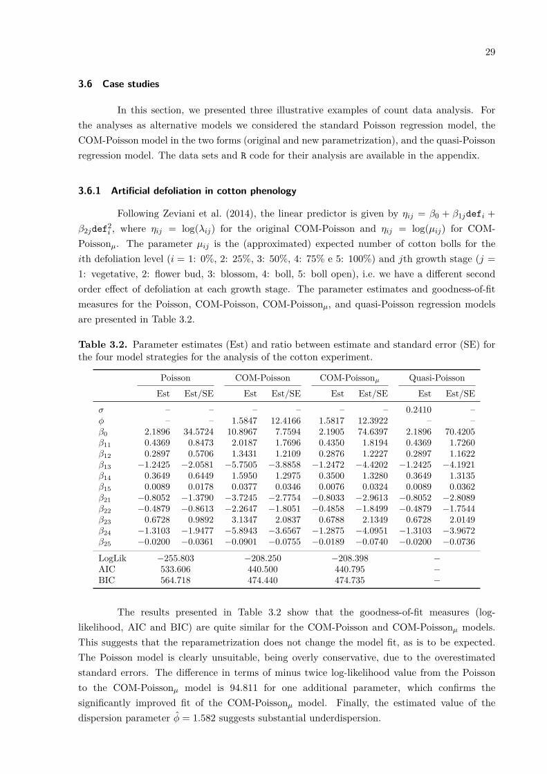
29
3.6 Case studies
In this section, we presented three illustrative examples of count data analysis. Forthe analyses as alternative models we considered the standard Poisson regression model, theCOM-Poisson model in the two forms (original and new parametrization), and the quasi-Poissonregression model. The data sets and R code for their analysis are available in the appendix.
3.6.1 Artificial defoliation in cotton phenology
Following Zeviani et al. (2014), the linear predictor is given by ηij = β0 + β1jdefi +β2jdef2
i , where ηij = log(λij) for the original COM-Poisson and ηij = log(µij) for COM-Poissonµ. The parameter µij is the (approximated) expected number of cotton bolls for theith defoliation level (i = 1: 0%, 2: 25%, 3: 50%, 4: 75% e 5: 100%) and jth growth stage (j =1: vegetative, 2: flower bud, 3: blossom, 4: boll, 5: boll open), i.e. we have a different secondorder effect of defoliation at each growth stage. The parameter estimates and goodness-of-fitmeasures for the Poisson, COM-Poisson, COM-Poissonµ, and quasi-Poisson regression modelsare presented in Table 3.2.
Table 3.2. Parameter estimates (Est) and ratio between estimate and standard error (SE) forthe four model strategies for the analysis of the cotton experiment.
Poisson COM-Poisson COM-Poissonµ Quasi-PoissonEst Est/SE Est Est/SE Est Est/SE Est Est/SE
σ – – – – – – 0.2410 –ϕ – – 1.5847 12.4166 1.5817 12.3922 – –β0 2.1896 34.5724 10.8967 7.7594 2.1905 74.6397 2.1896 70.4205β11 0.4369 0.8473 2.0187 1.7696 0.4350 1.8194 0.4369 1.7260β12 0.2897 0.5706 1.3431 1.2109 0.2876 1.2227 0.2897 1.1622β13 −1.2425 −2.0581 −5.7505 −3.8858 −1.2472 −4.4202 −1.2425 −4.1921β14 0.3649 0.6449 1.5950 1.2975 0.3500 1.3280 0.3649 1.3135β15 0.0089 0.0178 0.0377 0.0346 0.0076 0.0324 0.0089 0.0362β21 −0.8052 −1.3790 −3.7245 −2.7754 −0.8033 −2.9613 −0.8052 −2.8089β22 −0.4879 −0.8613 −2.2647 −1.8051 −0.4858 −1.8499 −0.4879 −1.7544β23 0.6728 0.9892 3.1347 2.0837 0.6788 2.1349 0.6728 2.0149β24 −1.3103 −1.9477 −5.8943 −3.6567 −1.2875 −4.0951 −1.3103 −3.9672β25 −0.0200 −0.0361 −0.0901 −0.0755 −0.0189 −0.0740 −0.0200 −0.0736
LogLik −255.803 −208.250 −208.398 −AIC 533.606 440.500 440.795 −BIC 564.718 474.440 474.735 −
The results presented in Table 3.2 show that the goodness-of-fit measures (log-likelihood, AIC and BIC) are quite similar for the COM-Poisson and COM-Poissonµ models.This suggests that the reparametrization does not change the model fit, as is to be expected.The Poisson model is clearly unsuitable, being overly conservative, due to the overestimatedstandard errors. The difference in terms of minus twice log-likelihood value from the Poissonto the COM-Poissonµ model is 94.811 for one additional parameter, which confirms thesignificantly improved fit of the COM-Poissonµ model. Finally, the estimated value of thedispersion parameter ϕ̂ = 1.582 suggests substantial underdispersion.
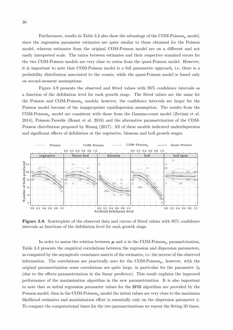
30
Furthermore, results in Table 3.2 also show the advantage of the COM-Poissonµ model,since the regression parameter estimates are quite similar to those obtained for the Poissonmodel, whereas estimates from the original COM-Poisson model are on a different and noteasily interpreted scale. The ratios between estimates and their respective standard errors forthe two COM-Poisson models are very close to ratios from the quasi-Poisson model. However,it is important to note that COM-Poisson model is a full parametric approach, i.e. there is aprobability distribution associated to the counts, while the quasi-Poisson model is based onlyon second-moment assumptions.
Figure 3.9 presents the observed and fitted values with 95% confidence intervals asa function of the defoliation level for each growth stage. The fitted values are the same forthe Poisson and COM-Poissonµ models, however, the confidence intervals are larger for thePoisson model because of the inappropriate equidispersion assumption. The results from theCOM-Poissonµ model are consistent with those from the Gamma-count model (Zeviani et al.2014), Poisson-Tweedie (Bonat et al. 2018) and the alternative parametrization of the COM-Poisson distribution proposed by Huang (2017). All of these models indicated underdispersionand significant effects of defoliation at the vegetative, blossom and boll growth stages.
Artificial defoliation level
Num
ber
of b
olls
pro
duc
ed
2
4
6
8
10
12
0.0 0.2 0.4 0.6 0.8 1.0
vegetative0.0 0.2 0.4 0.6 0.8 1.0
flower bud
0.0 0.2 0.4 0.6 0.8 1.0
blossom0.0 0.2 0.4 0.6 0.8 1.0
boll
0.0 0.2 0.4 0.6 0.8 1.0
boll open
Poisson COM−Poisson COM−Poissonµ Quasi−Poisson
Figure 3.9. Scatterplots of the observed data and curves of fitted values with 95% confidenceintervals as functions of the defoliation level for each growth stage.
In order to assess the relation between µ and ϕ in the COM-Poissonµ parametrization,Table 3.3 presents the empirical correlations between the regression and dispersion parameters,as computed by the asymptotic covariance matrix of the estimates, i.e. the inverse of the observedinformation. The correlations are practically zero for the COM-Poissonµ, however, with theoriginal parametrization some correlations are quite large, in particular for the parameter β0
(due to the effects parametrization in the linear predictor). This result explains the improvedperformance of the maximization algorithm in the new parametrization. It is also importantto note that as initial regression parameter values for the BFGS algorithm are provided by thePoisson model, then in the COM-Poissonµ model the initial values are very close to the maximumlikelihood estimates and maximization effort is essentially only on the dispersion parameter ϕ.To compare the computational times for the two parametrizations we repeat the fitting 50 times.
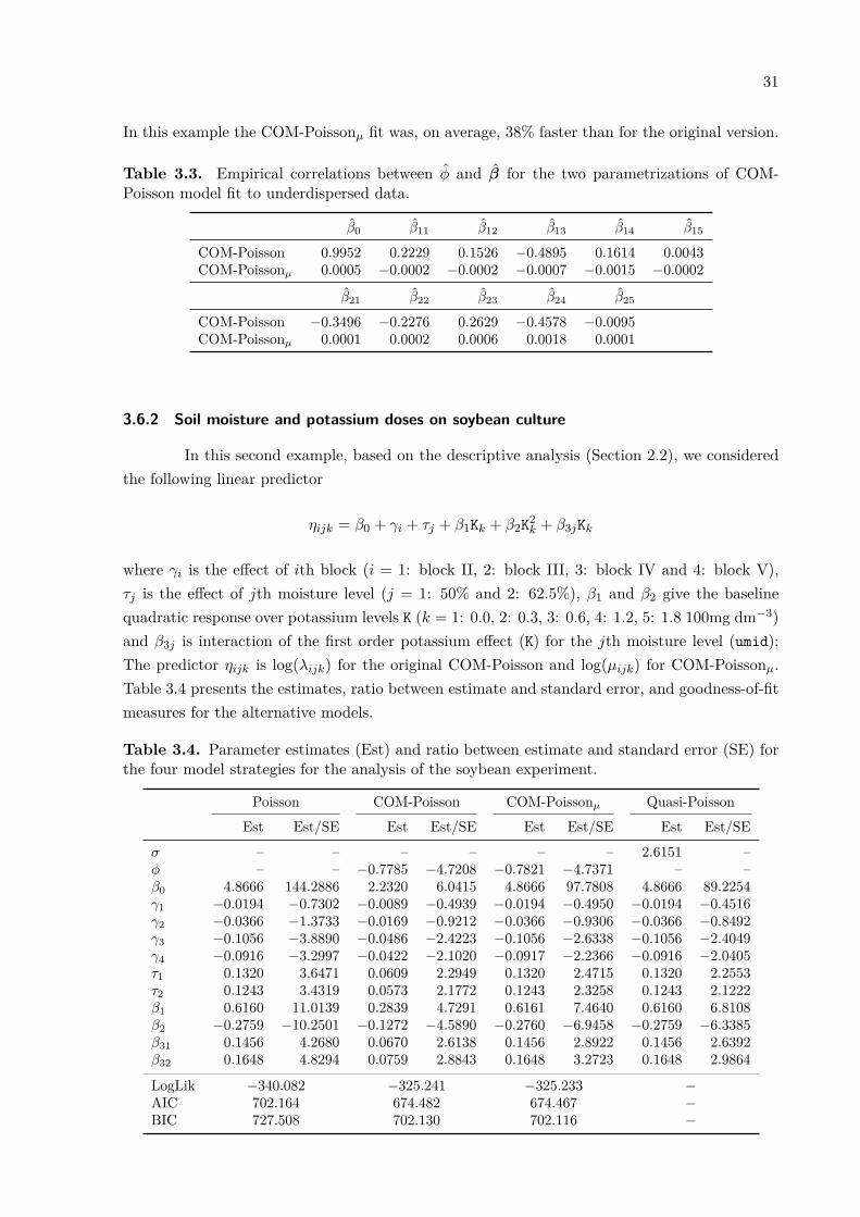
31
In this example the COM-Poissonµ fit was, on average, 38% faster than for the original version.
Table 3.3. Empirical correlations between ϕ̂ and β̂ for the two parametrizations of COM-Poisson model fit to underdispersed data.
β̂0 β̂11 β̂12 β̂13 β̂14 β̂15
COM-Poisson 0.9952 0.2229 0.1526 −0.4895 0.1614 0.0043COM-Poissonµ 0.0005 −0.0002 −0.0002 −0.0007 −0.0015 −0.0002
β̂21 β̂22 β̂23 β̂24 β̂25
COM-Poisson −0.3496 −0.2276 0.2629 −0.4578 −0.0095COM-Poissonµ 0.0001 0.0002 0.0006 0.0018 0.0001
3.6.2 Soil moisture and potassium doses on soybean culture
In this second example, based on the descriptive analysis (Section 2.2), we consideredthe following linear predictor
ηijk = β0 + γi + τj + β1Kk + β2K2k + β3jKk
where γi is the effect of ith block (i = 1: block II, 2: block III, 3: block IV and 4: block V),τj is the effect of jth moisture level (j = 1: 50% and 2: 62.5%), β1 and β2 give the baselinequadratic response over potassium levels K (k = 1: 0.0, 2: 0.3, 3: 0.6, 4: 1.2, 5: 1.8 100mg dm−3)and β3j is interaction of the first order potassium effect (K) for the jth moisture level (umid);The predictor ηijk is log(λijk) for the original COM-Poisson and log(µijk) for COM-Poissonµ.Table 3.4 presents the estimates, ratio between estimate and standard error, and goodness-of-fitmeasures for the alternative models.
Table 3.4. Parameter estimates (Est) and ratio between estimate and standard error (SE) forthe four model strategies for the analysis of the soybean experiment.
Poisson COM-Poisson COM-Poissonµ Quasi-PoissonEst Est/SE Est Est/SE Est Est/SE Est Est/SE
σ – – – – – – 2.6151 –ϕ – – −0.7785 −4.7208 −0.7821 −4.7371 – –β0 4.8666 144.2886 2.2320 6.0415 4.8666 97.7808 4.8666 89.2254γ1 −0.0194 −0.7302 −0.0089 −0.4939 −0.0194 −0.4950 −0.0194 −0.4516γ2 −0.0366 −1.3733 −0.0169 −0.9212 −0.0366 −0.9306 −0.0366 −0.8492γ3 −0.1056 −3.8890 −0.0486 −2.4223 −0.1056 −2.6338 −0.1056 −2.4049γ4 −0.0916 −3.2997 −0.0422 −2.1020 −0.0917 −2.2366 −0.0916 −2.0405τ1 0.1320 3.6471 0.0609 2.2949 0.1320 2.4715 0.1320 2.2553τ2 0.1243 3.4319 0.0573 2.1772 0.1243 2.3258 0.1243 2.1222β1 0.6160 11.0139 0.2839 4.7291 0.6161 7.4640 0.6160 6.8108β2 −0.2759 −10.2501 −0.1272 −4.5890 −0.2760 −6.9458 −0.2759 −6.3385β31 0.1456 4.2680 0.0670 2.6138 0.1456 2.8922 0.1456 2.6392β32 0.1648 4.8294 0.0759 2.8843 0.1648 3.2723 0.1648 2.9864
LogLik −340.082 −325.241 −325.233 −AIC 702.164 674.482 674.467 −BIC 727.508 702.130 702.116 −
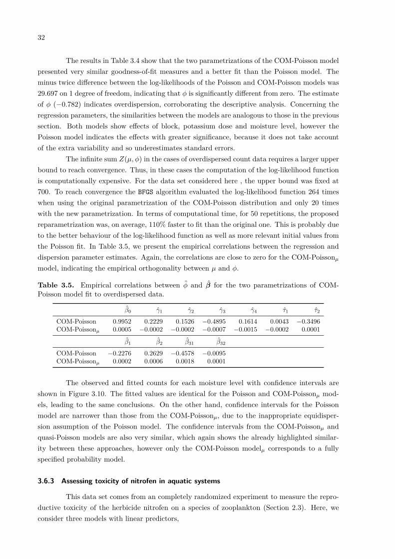
32
The results in Table 3.4 show that the two parametrizations of the COM-Poisson modelpresented very similar goodness-of-fit measures and a better fit than the Poisson model. Theminus twice difference between the log-likelihoods of the Poisson and COM-Poisson models was29.697 on 1 degree of freedom, indicating that ϕ is significantly different from zero. The estimateof ϕ (−0.782) indicates overdispersion, corroborating the descriptive analysis. Concerning theregression parameters, the similarities between the models are analogous to those in the previoussection. Both models show effects of block, potassium dose and moisture level, however thePoisson model indicates the effects with greater significance, because it does not take accountof the extra variability and so underestimates standard errors.
The infinite sum Z(µ, ϕ) in the cases of overdispersed count data requires a larger upperbound to reach convergence. Thus, in these cases the computation of the log-likelihood functionis computationally expensive. For the data set considered here , the upper bound was fixed at700. To reach convergence the BFGS algorithm evaluated the log-likelihood function 264 timeswhen using the original parametrization of the COM-Poisson distribution and only 20 timeswith the new parametrization. In terms of computational time, for 50 repetitions, the proposedreparametrization was, on average, 110% faster to fit than the original one. This is probably dueto the better behaviour of the log-likelihood function as well as more relevant initial values fromthe Poisson fit. In Table 3.5, we present the empirical correlations between the regression anddispersion parameter estimates. Again, the correlations are close to zero for the COM-Poissonµ
model, indicating the empirical orthogonality between µ and ϕ.
Table 3.5. Empirical correlations between ϕ̂ and β̂ for the two parametrizations of COM-Poisson model fit to overdispersed data.
β̂0 γ̂1 γ̂2 γ̂3 γ̂4 τ̂1 τ̂2
COM-Poisson 0.9952 0.2229 0.1526 −0.4895 0.1614 0.0043 −0.3496COM-Poissonµ 0.0005 −0.0002 −0.0002 −0.0007 −0.0015 −0.0002 0.0001
β̂1 β̂2 β̂31 β̂32
COM-Poisson −0.2276 0.2629 −0.4578 −0.0095COM-Poissonµ 0.0002 0.0006 0.0018 0.0001
The observed and fitted counts for each moisture level with confidence intervals areshown in Figure 3.10. The fitted values are identical for the Poisson and COM-Poissonµ mod-els, leading to the same conclusions. On the other hand, confidence intervals for the Poissonmodel are narrower than those from the COM-Poissonµ, due to the inappropriate equidisper-sion assumption of the Poisson model. The confidence intervals from the COM-Poissonµ andquasi-Poisson models are also very similar, which again shows the already highlighted similar-ity between these approaches, however only the COM-Poisson modelµ corresponds to a fullyspecified probability model.
3.6.3 Assessing toxicity of nitrofen in aquatic systems
This data set comes from an completely randomized experiment to measure the repro-ductive toxicity of the herbicide nitrofen on a species of zooplankton (Section 2.3). Here, weconsider three models with linear predictors,
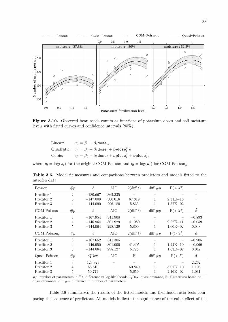
33
Potassium fertilization level
Num
ber
of g
rain
s pe
r po
t
100
150
200
250
0.0 0.5 1.0 1.5
: moisture 37.5%0.0 0.5 1.0 1.5
: moisture 50%
0.0 0.5 1.0 1.5
: moisture 62.5%
Poisson COM−Poisson COM−Poissonµ Quasi−Poisson
Figure 3.10. Observed bean seeds counts as functions of potassium doses and soil moisturelevels with fitted curves and confidence intervals (95%).
Linear: ηi = β0 + β1dosei,Quadratic: ηi = β0 + β1dosei + β2dose2
i eCubic: ηi = β0 + β1dosei + β2dose2
i + β3dose3i ,
where ηi = log(λi) for the original COM-Poisson and ηi = log(µi) for COM-Poissonµ.
Table 3.6. Model fit measures and comparisons between predictors and models fitted to thenitrofen data.
Poisson #p ℓ AIC 2(diff ℓ) diff #p P(> χ2)Preditor 1 2 −180.667 365.335 – – – –Preditor 2 3 −147.008 300.016 67.319 1 2.31E−16 –Preditor 3 4 −144.090 296.180 5.835 1 1.57E−02 –
COM-Poisson #p ℓ AIC 2(diff ℓ) diff #p P(> χ2) ϕ̂
Preditor 1 3 −167.954 341.908 – – – −0.893Preditor 2 4 −146.964 301.929 41.980 1 9.22E−11 −0.059Preditor 3 5 −144.064 298.129 5.800 1 1.60E−02 0.048
COM-Poissonµ #p ℓ AIC 2(diff ℓ) diff #p P(> χ2) ϕ̂
Preditor 1 3 −167.652 341.305 – – – −0.905Preditor 2 4 −146.950 301.900 41.405 1 1.24E−10 −0.069Preditor 3 5 −144.064 298.127 5.773 1 1.63E−02 0.047Quasi-Poisson #p QDev AIC F diff #p P(> F ) σ̂
Preditor 1 3 123.929 – – – – 2.262Preditor 2 4 56.610 – 60.840 1 5.07E−10 1.106Preditor 3 5 50.774 – 5.659 1 2.16E−02 1.031
#p, number of parameters; diff ℓ, difference in log-likelihoods; QDev, quasi-deviance, F, F statistics based onquasi-deviances; diff #p, difference in number of parameters.
Table 3.6 summarizes the results of the fitted models and likelihood ratio tests com-paring the sequence of predictors. All models indicate the significance of the cubic effect of the

34
nitrofen concentration. Considering this predictor, there is evidence of equidispersed counts, theϕ estimate of the COM-Poisson is close to zero and the σ estimate of the quasi-Poisson is closeto one. It is interesting to note that if we omit the higher order effects the models show evidenceof overdispersion — this exemplifies the discussion on the possible causes of overdispersion inSection 3.1. We also note that the quasi-Poisson approach, although robust to the equidispersionassumption, shows higher descriptive levels (p-values) than parametric models, that is, the testsunder parametric models are more powerful than the ones under the quasi-Poisson model in theequidispersed case.
In Table 3.7, we present the estimates of the regression parameters for the cubic dosemodels. The interpretations are similar to the other case studies, however, here the Poissonmodel is also suitable for indicating the significance of the covariate effects. In addition, notethat the parameter estimates of the original COM-Poisson model are comparable to the othersmodels. This occurs because we are in the particular case, where ϕ ≈ 0, which implies λ ≈ µ.
Table 3.7. Parameter estimates (Est) and ratio between estimate and standard error (SE) forthe four cubic dose models for the analysis of the nitrofen experiment.
Poisson COM-Poisson COM-Poissonµ Quasi-PoissonEst Est/SE Est Est/SE Est Est/SE Est Est/SE
β0 3.4767 62.8167 3.6494 4.8499 3.4769 64.3083 3.4767 61.8599β1 −0.0860 −0.4328 −0.0914 −0.4475 −0.0879 −0.4523 −0.0860 −0.4262β2 0.1529 0.8634 0.1612 0.8783 0.1547 0.8938 0.1529 0.8502β3 −0.0972 −2.3978 −0.1021 −2.2294 −0.0976 −2.4635 −0.0972 −2.3612
Figure 3.11 shows the number of live off-spring observed and fitted curves along withconfidence intervals for the different cubic dose models. The fitted values and confidence intervalsare identical and have a complete overlap. This shows that the estimation of the extra dispersionparameter does not affect the estimation of the regression coefficients in the case of equidispersedcounts.
Finally, in Table 3.8 we present the empirical correlations between the regression anddispersion parameter estimates. The results show that even in the special case (ϕ = 0), theempirical correlations for the original COM-Poisson model are not zero. For the reparametrizedmodel, as discussed in the previous sections, the correlations are practically null. The compu-tational times for fifty repetitions of fit are similar; the average time to fit the COM-Poissonµ
and COM-Poisson models is 1.19 and 1.09 seconds, respectively.
Table 3.8. Empirical correlations between ϕ̂ and β̂ for the two parametrizations of COM-Poisson model fit to equidispersed data.
β̂0 β̂1 β̂2 β̂3
COM-Poisson 0.9972 −0.0771 0.1562 −0.4223COM-Poissonµ −0.0003 0.0023 −0.0029 0.0033

35
Nitrofen concentration level
Num
ber
of li
ve o
ffsp
ring
0
10
20
30
0 1 2 3
PoissonCOM−Poisson
COM−Poissonµ
Quasi−Poisson
Figure 3.11. Number of live offspring observed for each nitrofen concentration level with fittedcurves and 95% confidence intervals.
3.7 Concluding remarks
In this chapter, we presented and characterized a novel reparametrization of the COM-Poisson distribution and associated regression model. The reparametrization was based on asimple asymptotic approximation for the expectation of the COM-Poisson distribution. Themain advantage of the proposed reparametrization is the simple interpretation of the regressioncoefficients in terms of the (approximate) expectation of the response variable as usual in thegeneralized linear models context. Thus, it is possible to compare directly the results from theCOM-Poisson model with those from standard approaches, such as the Poisson and quasi-Poissonregression models. Furthermore, in the new parametrization the COM-Poisson distribution isindexed by µ and an extra dispersion parameter ϕ which our studies suggest are approximatelyorthogonal. Overall the approach is similar to Huang’s (2017) parametrization but ours issimpler, because the µ used here is obtained from simple algebra.
The proposed parametrization is always valid, only the interpretation of the µ param-eter, as the expectation of the distribution, depends on the accuracy of the approximation. Weevaluated the accuracy of the approximations for the expectation and variance of the COM-Poisson distribution by considering quadratic approximation errors. We found that the meanapproximation is slightly inaccurate only for strongly overdispersed counts with small averages.Therefore, otherwise, the mean approximation is reasonable and the regression coefficients canbe interpreted in terms of expectation. In this situation the parameter estimates from the COM-Poisson model will be very close to those from the Poisson (and quasi-Poisson) fit, as was seenin the case studies, and this agreement can be considered as an indication of the reasonablenessof the approximation.
We discuss the properties and flexibility of the distribution to deal with count datathrough considerations of dispersion, zero-inflation and heavy-tail indexes. A simulation studywas used to assess the properties of the reparametrized COM-Poisson model and its ability todeal with different levels of dispersion, as well as the properties of the maximum likelihood
36
estimators. The results of our simulation study suggested that the maximum likelihood esti-mators of the regression and dispersion parameters are unbiased and consistent. The empiricalcoverage rates of the confidence intervals computed based on the asymptotic distribution of themaximum likelihood estimators are close to the nominal level for sample sizes greater than 100.The worst case scenario is when we have a small sample size and strongly overdispersed counts.In general, we recommend the use of the asymptotic confidence intervals for computational sim-plicity, although of course bootstrap intervals could be obtained, but would involve extensivecomputation.
The three examples and data analyses have shown that the COM-Poisson regressionmodel is a suitable choice to deal with generally dispersed count data, equi-, under- and over-dispersed. The observed empirical correlation between the regression and dispersion param-eter estimators and deviance surfaces suggest approximate orthogonality between µ and ϕ inthe COM-Poissonµ distribution. Thus, the computational procedure based on the proposedreparametrization is faster than that for the original parametrization.
In general, the results presented by the reparametrized COM-Poisson models weresatisfactory and comparable to the conventional approaches. Therefore, its use in the analysis ofcount data is encouraged. The computational routines for fitting the original and reparametrizedCOM-Poisson regression models are available in the appendix.
References References
Bonat, W. H., B. Jørgensen, C. C. Kokonendji, and J. Hinde (2018). “Extended Poisson-Tweedie:properties and regression model for count data”. In: Statistical Modelling 18.1, pp. 24–49.
Chatla, S. B. and G. Shmueli (2018). “Efficient estimation of COM-Poisson regression and ageneralized additive model”. In: Computational Statistics & Data Analysis 121, pp. 71–89.
Cox, D. R. and N. Reid (1987). “Orthogonality and Approximate Conditional Inference (withdiscussion)”. In: Journal of the Royal Statistical Society. Series B (Methodological) 49.1, pp. 1–39.
Daly, F. and R. Gaunt (2016). “The Conway-Maxwell-Poisson distribution: Distributional theoryand approximation”. In: ALEA, Latin American Journal of Probability and MathematicalStatistics 13, pp. 635–658.
Gaunt, R., S. Iyengar, A. Olde Daalhuis, and B. Simsek (2017). “An asymptotic expansionfor the normalizing constant of the Conway-Maxwell-Poisson distribution”. In: Annals of theInstitute of Statistical Mathematics to appear.
Huang, A. (2017). “Mean-parametrized Conway–Maxwell–Poisson regression models for dis-persed counts”. In: Statistical Modelling 17.6, pp. 1–22.
Lord, D., S. R. Geedipally, and S. D. Guikema (2010). “Extension of the application of Conway-Maxwell-Poisson models: Analyzing traffic crash data exhibiting underdispersion”. In: RiskAnalysis 30.8, pp. 1268–1276.
Nocedal, J. and S. J. Wright (2006). Numerical optimization. 2nd edition. Series in OperationsResearch. New York: Springer, p. 636. isbn: 0387987932.
37
Pawitan, Y. (2001). In all likelihood: statistical modelling and inference using likelihood. NewYork: Oxford University Press.
Puig, P. and J. Valero (2006). “Count data distributions: some characterizations with applica-tions”. In: Journal of the American Statistical Association 101.473, pp. 332–340.
R Core Team (2017). R: A Language and Environment for Statistical Computing. R Foundationfor Statistical Computing. Vienna, Austria.
Ross, G. J. S. (1970). “The Efficient Use of Function Minimization in Non-Linear Maximum-Likelihood Estimation”. In: Journal of the Royal Statistical Society. Series C (Applied Statis-tics) 19.3, pp. 205–221.
Sellers, K. F. and G. Shmueli (2010). “A flexible regression model for count data”. In: Annals ofApplied Statistics 4.2, pp. 943–961.
Shmueli, G., T. P. Minka, J. B. Kadane, S. Borle, and P. Boatwright (2005). “A useful dis-tribution for fitting discrete data: Revival of the Conway-Maxwell-Poisson distribution”. In:Journal of the Royal Statistical Society. Series C (Applied Statistics) 54.1, pp. 127–142.
Wedderburn, R. W. M. (1974). “Quasi-Likelihood Functions, Generalized Linear Models, andthe Gauss-Newton Method”. In: Biometrika 61.3, p. 439.
Zeviani, W. M., P. J. Ribeiro Jr, W. H. Bonat, S. E. Shimakura, and J. A. Muniz (2014). “TheGamma-count distribution in the analysis of experimental underdispersed data”. In: Journalof Applied Statistics 41.12, pp. 2616–2626.

38

39
4 A REVIEW OF FLEXIBLE MODELS FOR DISPERSED COUNT DATA
ABSTRACT
In the analysis of count data often the equidispersion assumption is not suitable, hencethe Poisson regression model is inappropriate. Several count distributions that can handleboth under- and overdispersion have been proposed in the literature. However, a comparisonof these distributions in the context of regression models has not yet been performed. Inthis chapter, we reviewed and compared the use of COM-Poisson, Gamma-count, discreteWeibull, generalized Poisson, double Poisson and Poisson-Tweedie distributions for practi-cal data analysis. The main properties of the distributions are highlighted and comparedconsidering the dispersion, zero-inflation, and heavy-tail indexes. The application of thesemodels is illustrated with the analysis of two experimental data sets. The computationalroutines for fitting the models and the data sets are available in the appendix.
Keywords: COM-Poisson, Gamma-count, Generalized Poisson, Overdispersion, Poisson-Tweedie family, Underdispersion.
4.1 Introduction
Important advances for count data analysis have been reported in the literature. Amongthem, we mention, mainly, methods to model different levels of dispersion, since the standardPoisson model forces the equality between mean and variance, referred to as equidispersion,which rarely occurs in real data (Molenberghs, Verbeke, and Demétrio 2007). A comprehensivereview of new methods for modeling count data can be found in the recent monographs byWinkelmann (2008), Cameron and Trivedi (2013), and Hilbe (2014).
The most common failure of the equidispersion assumption is the overdispersion (orextra-Poisson variability) when the variance exceeds the mean. Overdispersion count data hasbeen well studied by the statistical community and there is a wide range of models to dealwith. Hinde and Demétrio (1998), for example, discussed models and estimation algorithms foroverdispersed discrete data, as the common choices negative binomial and quasi-Poisson. On theother hand, underdispersion, when the variance is smaller than the mean, is less often reportedin the literature. However, in the last decade, it has been of increasing interest.
Shmueli et al. (2005) brought back the COM-Poisson model and supported severalfurther research like as Lord, Guikema, and Geedipally (2008), Sellers and Shmueli (2010),Huang (2017), and Ribeiro Jr et al. (2018). Zeviani et al. (2014) discussed the analysis ofexperimental data based on the Gamma-count distribution. Klakattawi, Vinciotti, and Yu(2018) discussed the properties and application of the discrete Weibull distribution and Luyts etal. (2018) extended it to model longitudinal/clustered data. Zamani and Ismail (2012) presentedan extension for the generalized Poisson regression model. Double Poisson distribution proposedby Efron (1986), can be used as the distribution for the response variable in general purposedclass of models GAMLSS (generalized additive models for location, scale, and shape) (Rigby andStasinopoulos 2005). Bonat et al. (2018) proposed the extended Poisson-Tweedie for handlingunder- and overdispersion count data based on moments of the Poisson-Tweedie family.
40
The main goal of this chapter is to compare several model strategies for analysis ofdispersed count data, namely COM-Poisson, Gamma-count, discrete Weibull, generalized Pois-son, double Poisson, and Poisson-Tweedie, in terms of characteristic indexes (dispersion, zero-inflation, and heavy-tail) and real applications. Related work can be found in Kokonendji (2014)who did a well-documented discussion of count statistical models, but without applications ormodel comparisons, and Sellers and Morris (2017) who discussed the causes of underdispersionand presented some count distributions with two applications.
This chapter is organized in six sections. The considered model strategies and theirmain properties are presented in Section 4.2. In Section 4.3, we present the characteristic indexesand use them to compare the models. The regression models and estimation are presented inSection 4.4. Section 4.5 is devoted to illustrating the application of the models for analysisof two datasets results from experimental studies and compare the results. Finally, discussionand direction for future work are given in Section 4.6. The computational routines used in thischapter are available in the appendix.
4.2 Background
In this section, we shall introduce some count distributions taking into account dis-persed count data. Namely, we consider the COM-Poisson, Gamma-count, discrete Weibull,generalized Poisson, double Poisson, and Poisson-Tweedie distributions. We focus on the gene-sis of generating probability distributions and their main properties.
4.2.1 COM-Poisson distribution
The COM-Poisson distribution is an important member of the family of weighted Pois-son distributions (WPD) (Del Castillo and Pérez-Casany 1998). The WPD family weights thePoisson probability function by a suitable function, allowing for a nonlinear decrease in ratios ofsuccessive probabilities. A random variable Y is a weighted Poisson distribution if its probabilitymass function can be written in the form
Pr(Y = y) = exp(−λ)λy
y!w(y)
Eλ[w(Y )], y ∈ N,
where Eλ(·) denotes the mean value with respect to the Poisson random variable with parameterλ ≥ 0 and w(·) is a weight function. The weight function may depend on an extra parameter toensure more flexibility.
The COM-Poisson distribution arises when w(y) ≡ w(y, ν) = (y!)1−ν for ν ≥ 0 (Koko-nendji 2014). Its probability mass function takes the form
Pr(Y = y) = λy exp(−λ)(y!)νEλ[(Y !)1−ν ]
= λy
(y!)νZ(λ, ν), where Z(λ, ν) =
∞∑j=0
λj
(j!)ν. (4.1)
The series Z(λ, ν) is a normalizing constant that cannot be expressed in closed formunless for special cases. The parameters λ and ν have no direct interpretation but can be seen interms of the ratios of successive probabilities which is given, for the WPD family and particularlyfor the COM-Poisson distribution, by
Pr(Y = y − 1)Pr(Y = y)
= y
λ
w(y − 1)w(y)
CMP≡ yν
λ,
41
a nonlinear function of y. As the dispersion parameter, for 0 < ν < 1 and ν > 1 we havethe over- and underdispersion, respectively. When ν = 1 the Poisson distribution results as aspecial case. Another special case is the geometric distribution, when ν = 0 and λ < 1 withPr(Y = y) = λy(1 − λ). As a limiting case, the Bernoulli distribution arises when ν → ∞, withprobability of success equal to λ/(λ+ 1).
The COM-Poisson also belongs to the family of two-parameter power series distribu-tions (Johnson, Kemp, and Kotz 2005) and using the properties for this family, the mean andvariance of COM-Poisson distributions are given by
E(Y ) = λd
dλ[logZ(λ, ν)] and Var(Y ) = λ2 d
2
dλ2 [logZ(λ, ν)] + E(Y ),
respectively, but cannot be solved in closed form. Therefore, despite the nice properties of COM-Poisson distribution, its major limitation is that the location parameter λ does not representthe expectation of the distribution and has no direct interpretation. Under this motivation,Huang (2017) and Ribeiro Jr et al. (2018) proposed new parametrizations of COM-Poissondistribution related to the expectation. The distribution is now indexed by the parameter µ,where µ is obtained by the solution for ∑∞
j=0(j − µ)λj/(j!)ν = 0 in the Huang’s proposal andµ = λ1/ν − (ν − 1)/2ν in the Ribeiro Jr’s proposal. In this chapter, we use the Ribeiro Jr’sparametrization for simplicity.
4.2.2 Gamma-count distribution
Another straightforward flexible distribution arises from the relationship between Pois-son and exponential distribution. Following Winkelmann (1995), let τk > 0, k ∈ N∗, denote thewaiting times between the (k − 1)th and the kth event and ϑn, denote the arrival time of thenth event, so ϑn =
∑nk=1 τk. Finally, denote YT the number of events within a (0, T ) interval.
Following the definitions, we have
YT < y ⇐⇒ ϑy ≥ T
Pr(YT < y) = Pr(ϑy ≥ T ) = 1 − Fϑy (T ),
Pr(YT = y) = Pr(YT < y) − Pr(YT < y + 1)
Pr(YT = y) = Fϑy (T ) − Fϑy+1(T ),
(4.2)
where Fϑn(T ) is the cumulative density function of ϑn and T is the interval of the counting(offset). This process is called by renewal process (Cox 1962; Winkelmann 2008, p.54).
From the renewal process (4.2), Poisson distribution is obtained by assuming τk expo-nentially distributed. Consequently, ϑn drawn from an Erlang distribution (a special case ofgamma distribution) and Pr(YT = y) has closed form
Pr(YT = y) = Fϑy (T )−Fϑy+1(T ) =y−1∑j=0
exp(−λT )(λT )j
j!−
y∑j=0
exp(−λT )(λT )j
j!= exp(−λT )(λT )j
y!.
Winkelmann (1995) proposed to use a more general distribution for the waiting timesτk. The Gamma-count distribution assumes that τk is independently gamma distributed, i.e
42
τkiid∼ Gamma(α, β). Due to the reproductive property of gamma random variables, ϑn ∼
Gamma(yα, β). Thereby, the Gamma-count probability mass function takes the form
Pr(YT = y) =∫ T
0
βyαtyα−1
Γ(yα) exp(βt)dt−
∫ T
0
β(y+1)αt(y+1)α−1
Γ[(y + 1)α] exp(βt)dt, (4.3)
a difference between two gamma cumulative density functions, G(yα, β) −G((y+ 1)α, β), whereG(a, b) is the cumulative function Fϑy (T ) for the gamma variable with parameters a and b.
As in the COM-Poisson distribution, the moments cannot be obtained in closed form.However, Winkelmann (1995) using the results from Cox (1962), showed for increasing T ,i.e. high counts, it holds that
YTasy∼ N
(βT
α,βT
α2
),
thus the limiting variance-mean ratio equals a constant 1/α. Consequently, the Gamma-countdistribution displays overdispersion for 0 < α < 1 and underdispersion for α > 1.
In order to have a mean-type parameterization, we rewrite the Equation (4.3) in termsof κ = β/α, thus the probability mass function is given by
Pr(Y = y) = G(yα, κα) −G((y + 1)α, κβ). (4.4)
In this parametrization, the parameter κ is the expected value for the waiting times τk and notfor the counts, unless α = 1. However, for large T , the asymptotic distribution of Y holds andthe expected value of Y is equal to κT .
4.2.3 Discrete Weibull distribution
The discrete Weibull distribution comes from a discretization process of the continuousWeibull distribution (Nakagawa and Osaki 1975). Let T be a continuous Weibull distributedrandom variable with parameters λ > 0 and ρ > 0. The density function and cumulative densityfunction are, respectively, given by
fT (t) = λρtρ−1 exp(−λtρ) and FT (t) = 1 − exp(−λtρ).
The discrete Weibull distribution (type 1) (Nakagawa and Osaki 1975) is obtained by the prob-ability between two integer values on the suporte of continuous Weibull distribution. Let Y ∈ Nfollow a discrete Weibull distribution. Then its probability mass function is given by
Pr(Y = y) =∫ y+1
yfT (t)dt = FT (y + 1) − FT (y)
= exp(−λyρ) − exp(−λ(y + 1)ρ)
= qyρ − q(y+1)ρ,
(4.5)
where q = exp(−λ) ∈ (0, 1) and ρ > 0.The mean and variance of a discrete Weibull distribution are given by
E(Y ) =∞∑
j=1qjρ and Var(Y ) = 2
∞∑j=1
jqjρ − E(Y ) − E(Y )2,
for which there are no closed expressions (Klakattawi, Vinciotti, and Yu 2018).
43
This discretization method can be used to discretize any continuous distribution. Fromthe special cases of Weibull, we have correspondents specials cases of the discretized distribution:discrete exponential, when ρ = 1 (the popular geometric distribution) and discrete Rayleigh,when ρ = 2.
The main disadvantage of the discrete Weibull is that there is no easy interpretation ofthe model parameters q and ρ. In fact, there is no genuine dispersion and location parameter,the dispersion as well as the expectation is controlled by both q and ρ.
4.2.4 Generalized Poisson distribution
The generalized Poisson is another generalization of the Poisson distribution result-ing from the limiting form of the generalized negative binomial distribution (Consul and Jain1973). Let Y be a random variable according to the generalized Poisson distribution. Then itsprobability mass function is given by
Pr(Y = y) =
[λ(λ+ yγ)y−1 exp(−λ− yγ)
]/y!, y = 0, 1, 2, . . .
0 y > m,when γ < 0,(4.6)
where λ > 0, max(−1,−λ/4) ≤ γ ≤ 1 and m is the largest integer value for which λ+mγ > 0when γ is negative (Consul and Famoye 1992). The mean and variance is obtained by E(Y ) =λ(1 − γ)−1 and Var(Y ) = λ(1 − γ)−3. The Poisson distribution is a particular case when γ = 0.
To obtain the model in mean parametrization, let’s assume
λ = µ
1 + σµand γ = σµ
1 + σµ.
The resulting probability mass function can be written as
Pr(y) =(
µ
1 + σµ
)y (1 + σy)y−1
y!exp
[−µ (1 + σy)
(1 + σµ)
], (4.7)
where σ > min(−1/y,−1/µ), when σ < 0. The mean and variance under this parametrizationare given by
E(Y ) = µ and Var(Y ) = µ(1 + µσ)2. (4.8)
Thus, this distribution can model under-, when min(−1/y,−1/µ) < σ < 0 and overdispersion,when σ > 0. The Equation (4.7) reduces to the Poisson distribution when σ = 0. Regressionmodels based on the generalized Poisson are challenging by the presence of unusual parameterspace for underdispersion.
4.2.5 Double Poisson distribution
The double Poisson distribution has been proposed by Efron (1986) based on the doubleexponential family. Double exponential families allow the introduction of a second parameterthat controls variance independently of the mean. Following Efron (1986), a random variable Ydouble Poisson distributed has the probability mass function given by
Pr(Y = y) =√φ−1 exp
(−µ
φ
)(exp(−y)yy
y!
)(eµ
y
)y/φ 1K(µ, φ)
, (4.9)
44
where µ > 0, φ > 0 and K(µ, φ) is a normalizing constant that can be calculated as
K(µ, φ) =∞∑
j=0
√φ−1 exp
(−µ
φ
)(exp(−j)jj
j!
)(eµ
j
)j/φ
≈ 1 + φ− 112µ
(1 + φ
µ
). (4.10)
The closed form approximation to the K(µ, φ) (4.10) demostrated by Efron (1986) isreasonable for large values of µ, but is a poor approximation for small values (Zou, Geedipally,and Lord 2013).
The expected value and the variance referring to the double Poisson distribution haveno closed form, but Efron (1986) shows that it can be approximated as
E(Y ) ≈ µ and Var(Y ) ≈ φµ.
So, this distribution can model under- (0 < φ < 1), over- (φ > 1) and equidipersion (φ = 1,special case Poisson). The disadvantages of using double Poisson to count data analysis arerelated to the failure to obtain exact results and to the complexity of the normalizing constant(Lindsey 1996, sec. 2.3.3; Winkelmann 2008, sec. 2.6.4).
4.2.6 Poisson-Tweedie distribution
Poisson mixture models (Winkelmann 2008, sec. 2.5; Jørgensen 1997, sec. 4.6.1), alsocalled two-stage models (Hinde and Demétrio 1998) are widely applied to model overdispersedcount data. These models are specified hierarchically as Y ∼ Poisson(λ) and λ ∼ D(θ). Thestandard example for counts is the negative binomial distribution, where the mean parameter λis assumed to be gamma distributed.
A general case of Poisson mixture models is a Poisson-Tweedie case (Jørgensen 1997).The Poisson-Tweedie family is given by following the hierarchical specification
Y | Z ∼ Po(Z) with Z ∼ Twp(µ, ω), (4.11)
where Twp(µ, ω) denotes a Tweedie distribution, a proper exponential dispersion model (Jør-gensen 1997) with probability function given by
fZ(z;µ, ω, p) = a(z, ω, p) exp[(zψ − kp(ψ))/ω].
where µ = k′p(ψ) is the expectation, ω > 0 is the dispersion parameter, ψ is the canonical
parameter and kp(ψ) is the cumulant function. Furthermore, var(Z) = ωV (µ) where V (µ) =k′′
p(ψ) is the variance function. Tweedie densities are characterized by power variance functionsof the form V (µ) = µp, where p ∈ (−∞, 0] ∪ [1,∞). The support of the distribution depends onthe value of the power parameter. For p ≥ 2, 1 < p < 2 and p = 0 the support corresponds tothe positive, non-negative and real values, respectively.
The probability mass function for the Poisson-Tweedie for p > 1 is given by integratingout z, that is
Pr(Y = y) =∫ ∞
0
zy exp(−z)y!
a(z, ω, p) exp[(zψ − kp(ψ))/ω]dz. (4.12)
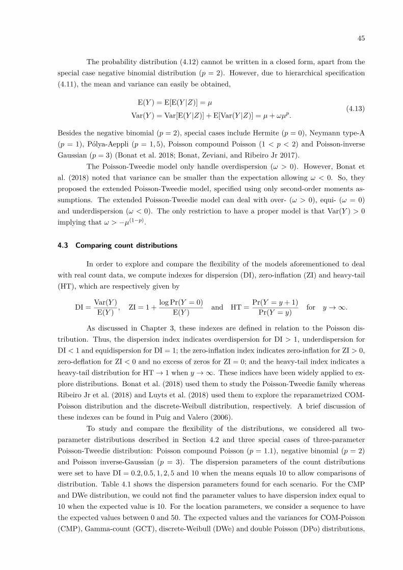
45
The probability distribution (4.12) cannot be written in a closed form, apart from thespecial case negative binomial distribution (p = 2). However, due to hierarchical specification(4.11), the mean and variance can easily be obtained,
E(Y ) = E[E(Y |Z)] = µ
Var(Y ) = Var[E(Y |Z)] + E[Var(Y |Z)] = µ+ ωµp.(4.13)
Besides the negative binomial (p = 2), special cases include Hermite (p = 0), Neymann type-A(p = 1), Pólya-Aeppli (p = 1, 5), Poisson compound Poisson (1 < p < 2) and Poisson-inverseGaussian (p = 3) (Bonat et al. 2018; Bonat, Zeviani, and Ribeiro Jr 2017).
The Poisson-Tweedie model only handle overdispersion (ω > 0). However, Bonat etal. (2018) noted that variance can be smaller than the expectation allowing ω < 0. So, theyproposed the extended Poisson-Tweedie model, specified using only second-order moments as-sumptions. The extended Poisson-Tweedie model can deal with over- (ω > 0), equi- (ω = 0)and underdispersion (ω < 0). The only restriction to have a proper model is that Var(Y ) > 0implying that ω > −µ(1−p).
4.3 Comparing count distributions
In order to explore and compare the flexibility of the models aforementioned to dealwith real count data, we compute indexes for dispersion (DI), zero-inflation (ZI) and heavy-tail(HT), which are respectively given by
DI = Var(Y )E(Y )
, ZI = 1 + log Pr(Y = 0)E(Y )
and HT = Pr(Y = y + 1)Pr(Y = y)
for y → ∞.
As discussed in Chapter 3, these indexes are defined in relation to the Poisson dis-tribution. Thus, the dispersion index indicates overdispersion for DI > 1, underdispersion forDI < 1 and equidispersion for DI = 1; the zero-inflation index indicates zero-inflation for ZI > 0,zero-deflation for ZI < 0 and no excess of zeros for ZI = 0; and the heavy-tail index indicates aheavy-tail distribution for HT → 1 when y → ∞. These indices have been widely applied to ex-plore distributions. Bonat et al. (2018) used them to study the Poisson-Tweedie family whereasRibeiro Jr et al. (2018) and Luyts et al. (2018) used them to explore the reparametrized COM-Poisson distribution and the discrete-Weibull distribution, respectively. A brief discussion ofthese indexes can be found in Puig and Valero (2006).
To study and compare the flexibility of the distributions, we considered all two-parameter distributions described in Section 4.2 and three special cases of three-parameterPoisson-Tweedie distribution: Poisson compound Poisson (p = 1.1), negative binomial (p = 2)and Poisson inverse-Gaussian (p = 3). The dispersion parameters of the count distributionswere set to have DI = 0.2, 0.5, 1, 2, 5 and 10 when the means equals 10 to allow comparisons ofdistribution. Table 4.1 shows the dispersion parameters found for each scenario. For the CMPand DWe distribution, we could not find the parameter values to have dispersion index equal to10 when the expected value is 10. For the location parameters, we consider a sequence to havethe expected values between 0 and 50. The expected values and the variances for COM-Poisson(CMP), Gamma-count (GCT), discrete-Weibull (DWe) and double Poisson (DPo) distributions,

46
Table 4.1. Dispersion Scenarios: dispersion parameters of CMP, GCT, DWe, GCT, GPo, DPo,and PTwp distributions when E(Y ) is set to 10 and DI(Y ) = 0.2, 0.5, 1, 2, 5, and 10.
Scenario 1 Scenario 2 Scenario 3 Scenario 4 Scenario 5 Scenario 6(DI = 0.2) (DI = 0.5) (DI = 1) (DI = 2) (DI = 5) (DI = 10)
CMP(ν) 5.2059 2.0526 1.0000 0.4687 0.1292 –GCT(α) 5.4221 2.0785 1.0000 0.4643 0.1370 0.0213DWe(ρ) 9.0735 5.4642 3.7150 2.5189 1.5145 –GPo(σ) −0.0553 −0.0293 0.0000 0.0414 0.1236 0.2162DPo(φ) 0.2001 0.5002 1.0000 1.9856 5.1625 13.9295
PTw1.1(ω) – – – 0.7943 3.1773 7.1490PTw2.0(ω) – – – 0.1000 0.4000 0.9000PTw3.0(ω) – – – 0.0100 0.0400 0.0900
are computed numerically using
E(Y ) =500∑y=0
yPr(Y = y) and Var(Y ) =500∑y=0
{[y − E(Y )]2} Pr(Y = y).
For the generalized Poisson (GPo) and Poisson-Tweedie (PTw) distributions, the expected valuesand the variances have closed forms (Equations (4.8) and (4.13)). To obtain the HT and ZI forthe Poisson-Tweedie distributions, we approximate the value of integral (4.12) using the Gauss-Laguerre method with 100 nodes, following the codes provide by Bonat et al. (2018). Since thePoisson-Tweedie cannot deal with underdispersion, in these scenarios we present only the otherdistributions. Figures 4.1, 4.2 and 4.3, display the indexes by the different scenarios.
(a)Expectation
Dis
pers
ion
ind
ex (D
I)
0
2
4
6
0 10 20 30 40 50
CMP(µ, φ)
(b)Expectation
Dis
pers
ion
ind
ex (D
I)
0
5
10
15
20
25
0 10 20 30 40 50
GCT(κ, α)
(c)
q parameter
Dis
pers
ion
ind
ex (D
I)
0
5
10
0.95 0.96 0.97 0.98 0.99
DWe(q, ρ)
(d)Expectation
Dis
pers
ion
ind
ex (D
I)
0
50
100
0 10 20 30 40 50
GPo(µ, σ)
(e)Expectation
Dis
pers
ion
ind
ex (D
I)
0
5
10
0 10 20 30 40 50
DPo(µ, φ)
(f)Expectation
Dis
pers
ion
ind
ex (D
I)
2
4
6
8
10
12
0 10 20 30 40 50
PTw1.1(µ, ω)
(g)Expectation
Dis
pers
ion
ind
ex (D
I)
0
10
20
30
40
0 10 20 30 40 50
PTw2(µ, ω)
(h)Expectation
Dis
pers
ion
ind
ex (D
I)
0
50
100
150
200
0 10 20 30 40 50
PTw3(µ, ω)
Scenario 1 Scenario 2 Scenario 3 Scenario 4 Scenario 5 Scenario 6
Figure 4.1. Dispersion index as function of expected values by different scenarios and countdistributions. Dotted lines (DI = 1) represent the Poisson distribution.
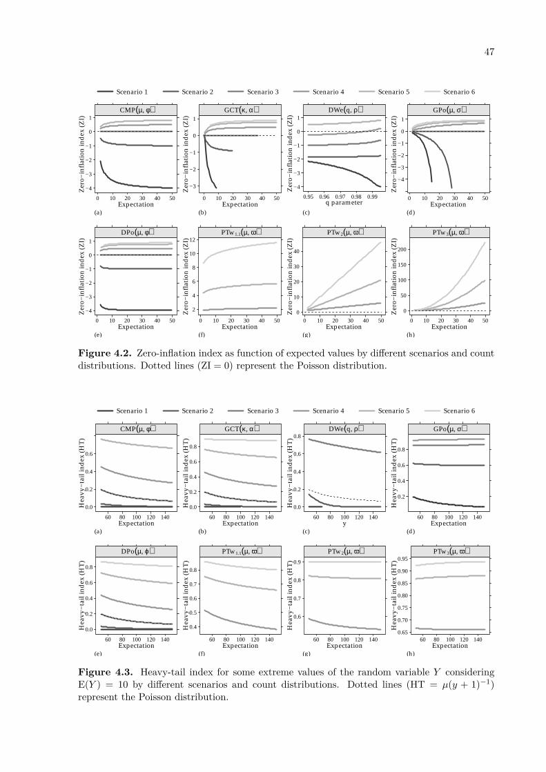
47
(a)Expectation
Zer
o−in
flat
ion
ind
ex (Z
I)
−4
−3
−2
−1
0
1
0 10 20 30 40 50
CMP(µ, φ)
(b)Expectation
Zer
o−in
flat
ion
ind
ex (Z
I)−3
−2
−1
0
1
0 10 20 30 40 50
GCT(κ, α)
(c)
q parameter
Zer
o−in
flat
ion
ind
ex (Z
I)
−4
−3
−2
−1
0
1
0.95 0.96 0.97 0.98 0.99
DWe(q, ρ)
(d)Expectation
Zer
o−in
flat
ion
ind
ex (Z
I)
−4
−3
−2
−1
0
1
0 10 20 30 40 50
GPo(µ, σ)
(e)Expectation
Zer
o−in
flat
ion
ind
ex (Z
I)
−4
−3
−2
−1
0
1
0 10 20 30 40 50
DPo(µ, φ)
(f)Expectation
Zer
o−in
flat
ion
ind
ex (Z
I)
2
4
6
8
10
12
0 10 20 30 40 50
PTw1.1(µ, ω)
(g)Expectation
Zer
o−in
flat
ion
ind
ex (Z
I)
0
10
20
30
40
0 10 20 30 40 50
PTw2(µ, ω)
(h)Expectation
Zer
o−in
flat
ion
ind
ex (Z
I)
0
50
100
150
200
0 10 20 30 40 50
PTw3(µ, ω)
Scenario 1 Scenario 2 Scenario 3 Scenario 4 Scenario 5 Scenario 6
Figure 4.2. Zero-inflation index as function of expected values by different scenarios and countdistributions. Dotted lines (ZI = 0) represent the Poisson distribution.
(a)Expectation
Hea
vy−
tail
ind
ex (H
T)
0.0
0.2
0.4
0.6
60 80 100 120 140
CMP(µ, φ)
(b)Expectation
Hea
vy−
tail
ind
ex (H
T)
0.0
0.2
0.4
0.6
0.8
60 80 100 120 140
GCT(κ, α)
(c)y
Hea
vy−
tail
ind
ex (H
T)
0.0
0.2
0.4
0.6
0.8
60 80 100 120 140
DWe(q, ρ)
(d)Expectation
Hea
vy−
tail
ind
ex (H
T)
0.2
0.4
0.6
0.8
60 80 100 120 140
GPo(µ, σ)
(e)Expectation
Hea
vy−
tail
ind
ex (H
T)
0.0
0.2
0.4
0.6
0.8
60 80 100 120 140
DPo(µ, ϕ)
(f)Expectation
Hea
vy−
tail
ind
ex (H
T)
0.4
0.5
0.6
0.7
0.8
60 80 100 120 140
PTw1.1(µ, ω)
(g)Expectation
Hea
vy−
tail
ind
ex (H
T)
0.6
0.7
0.8
0.9
60 80 100 120 140
PTw2(µ, ω)
(h)Expectation
Hea
vy−
tail
ind
ex (H
T)
0.65
0.70
0.75
0.80
0.85
0.90
0.95
60 80 100 120 140
PTw3(µ, ω)
Scenario 1 Scenario 2 Scenario 3 Scenario 4 Scenario 5 Scenario 6
Figure 4.3. Heavy-tail index for some extreme values of the random variable Y consideringE(Y ) = 10 by different scenarios and count distributions. Dotted lines (HT = µ(y + 1)−1)represent the Poisson distribution.
48
The DIs in Figure 4.1 show that the CMP, GCT, DPo, and PTw1.1 (only for overdis-persion) are quite similar. In general, for these distributions, the indexes depend slightly onthe expected values and tend to stabilize for large expected values. Consequently, the mean-variance relationship is proportional to the dispersion parameter value. In fact, if we look atthe (approximate) variances for these distributions, they follow the same structure. The DIsfor PTw3 and GPo distributions shows that distributions are suitable to handle very strongoverdispersion. For the DWe distribution, the x-axis is the q parameter, so the interpretation isnot straightforward.
The ZIs in Figure 4.2 show that CMP, GCT, DWe, GPo, and DPo can handle a limitedamount of zero-inflation, in cases of overdispersion (DI < 1) and it is suitable for zero-deflation,in cases of underdispersion (DI > 1). For the GCT distribution on the underdispersion scenarios(DI = 0.5 and DI = 0.5), the probability at zero tends to 0 as the mean increases, hence the ZI →−∞. That is why the curves are dropped for the GCT distribution. Also in the underdispersionscenarios, the shape of the curves for the GPo distribution is interesting. Analytically, the ZI forGPo distribution is (−1 −σµ)−1, which has a vertical asymptote at µ = −1/σ, limµ→−1/σ ZI(µ)is equals to −∞ from the left and ∞ from the right. However, there is no distribution whenµ > −1/σ (see Equation (4.7)). The ZI’s for PTw distributions increase quickly as the meanincreases, indicating that distributions are suitable to deal with zero-inflated count data.
Finally, HTs in Figure 4.3 indicates that CMP, GCT, DWe, DPo and PTw1.1 distri-butions are in general light-tailed distributions i.e. HT → 0 for y → ∞. Actually, the HT forthe DWe distributions tends to 1 for small values of the expectation (Luyts et al. 2018). Theindexes for GPo and PTwp (p = 1, 2) distributions increases with increasing mean, showing thatthe model is especially suitable to deal with heavy-tailed count data.
4.4 Regression models and estimation
Suppose yi, i = 1, . . . , n is a set of independents realizations of Yi according to distribu-tion D(., .) and xi a vector of known covariates. The regression models based on the distributionsaformentioned is defined by
Yi ∼ D(g−1(ηi), θ), with ηi = x⊤i β,
where θ is a general notation for the dispersion (or second) parameter of the distribution D andg(.) is a suitable link function.
Table 4.2 summarizes the main properties of the count distributions considered, presentsthe link functions adopted, and establishes the notation. Similar results (exact, approximatedor limiting) can be directly linked to the results presented in Figure 4.1.
Except for the Poisson-Tweedie, the parameter estimation is based on the maximumlikelihood method and the inference is done using the standard machinery of likelihood infer-ence, including likelihood ratio tests for model comparison and Wald-tests for testing individual(or groups of) parameters. Since the derivatives of the log-likelihood function cannot be ob-tained analytically for any of these models, we compute them by central finite differences usingthe Richardson method as implemented in package numDeriv (Gilbert and Varadhan 2016) inR (R Core Team 2018). The normalizing constants present in the COM-Poisson and double
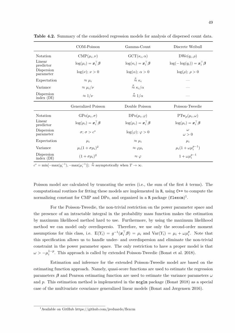
49
Table 4.2. Summary of the considered regression models for analysis of dispersed count data.
COM-Poisson Gamma-Count Discrete Weibull
Notation CMP(µi, ν) GCT(κi, α) DWe(qi, ρ)Linearpredictor log(µi) = x⊤
i β log(κi) = x⊤i β log(− log(qi)) = x⊤
i β
Dispersionparameter log(ν); ν > 0 log(α); α > 0 log(ρ); ρ > 0
Expectation ≈ µia≈ κi —
Variance ≈ µi/νa≈ κi/α —
Dispersionindex (DI) ≈ 1/ν
a≈ 1/α —
Generalized Poisson Double Poisson Poisson-Tweedie
Notation GPo(µi, σ) DPo(µi, φ) PTwp(µi, ω)Linearpredictor log(µi) = x⊤
i β log(µi) = x⊤i β log(µi) = x⊤
i β
Dispersionparameter σ; σ > c∗ log(φ); φ > 0 ω
ω > 0Expectation µi ≈ µi µi
Variance µi(1 + σµi)2 ≈ φµi µi(1 + ωµp−1i )
Dispersionindex (DI) (1 + σµi)2 ≈ φ 1 + ωµp−1
i
c∗ = min[−max(y−1i ), −max(µ−1
i )];a≈ asymptotically when T → ∞.
Poisson model are calculated by truncating the series (i.e., the sum of the first k terms). Thecomputational routines for fitting these models are implemented in R, using C++ to compute thenormalizing constant for CMP and DPo, and organized in a R package (flexcm)1.
For the Poisson-Tweedie, the non-trivial restriction on the power parameter space andthe presence of an intractable integral in the probability mass function makes the estimationby maximum likelihood method hard to use. Furthermore, by using the maximum likelihoodmethod we can model only overdispersio. Therefore, we use only the second-order momentassumptions for this class, i.e. E(Yi) = g−1(x⊤
i β) = µi and Var(Yi) = µi + ωµpi . Note that
this specification allows us to handle under- and overdispersion and eliminate the non-trivialconstraint in the power parameter space. The only restriction to have a proper model is thatω > −µ1−p
i . This approach is called by extended Poisson-Tweedie (Bonat et al. 2018).
Estimation and inference for the extended Poisson-Tweedie model are based on theestimating function approach. Namely, quasi-score functions are used to estimate the regressionparameters β and Pearson estimating function are used to estimate the variance parameters ωand p. This estimation method is implemented in the mcglm package (Bonat 2018) as a specialcase of the multivariate covariance generalized linear models (Bonat and Jørgensen 2016).
1Available on GitHub https://github.com/jreduardo/flexcm
50
4.5 Data analyses
In this section, we analyzed two data sets to illustrate and compare the applications ofthe flexible regression models. The data sets and R code for their analysis are available in theappendix.
4.5.1 Sitophilus zeamaus experiment
As the first example, we analyse the Sitophilus zeamaus data set introduced in Section2.5. This dataset results from a completely randomized experiment with ten replicates and fourtreatments. To analyze the number of insects (Yij), we consider the linear predictor ηij = β0+τj ,where i = 1, 2, . . . , 10 and j refers to the treatments (control, leaf, branch, and seed).
The parameter estimates, associated standard errors and goodness-of-fit measures(maximized log-likelihood and Akaike information criterion) are given in Table 4.3. Notethat for the PTw model, we could calculate the log-likelihood function since the estimatedparameters (p̂ = 1.4031 and ω̂ = 0.3476) correspond to an existing Poisson-Tweedie distribution.Furthermore, except for DWe model, all models have large improvements related to the standardPoisson model, whose maximum log-likelihood is equal to −130.5828. The likelihood ratio testsfor H0 : log(θ) = 0 (where θ is the associated dispersion parameter) for the models nesting thePoisson model (i.e. CMP, GCT, GPo, DPo and PTw) indicates strong evidence to reject thenull hypothesis.
In terms of practical inference, all models lead to the same conclusion – the extractprepared with seeds of Annano mucosa drastically decrease the Sitophilus zeamais progeny whilethe other solutions (control, leaves and branch) had the same effect (see regression coefficientsin Table 4.3). The same conclusion is reached by Demétrio, Hinde, and Moral (2014) using aquasi-Poisson specification (Wedderburn 1974).
Table 4.3 also shows the disadvantage of the DWe model in terms of interpretation.Whereas the others models are parameterized in terms of mean, even approximately or asymp-totically, the DWe model parameters are on a not easily interpretable scale.
Fitted counts with 95% confidence intervals for the six models are given in Figure4.4. The results are practically identical for CMP, GCT, GPo, DPo and PTw. Only for DWethe results are slightly lower than the values reported for the others. Thus, along with thelog-likelihoods presented in Table 4.3, it seems that the DWe model is not suitable to fit thisdataset.
Figure 4.4(b) shows the mean-variance relationship for the six fitted models. To obtainthese curves, we computed the expected values and the the variances for the location parametervarying from g−1(ηlwr) to g−1(ηupr) (lower and upper of the linear predictor confidence interval),and dispersion parameter fixed at the maximum likelihood estimate. The results show that thevariance increases linearly for CMP, GCT and DPo and polynomially for DWe, GPo and PTw.In fact, the polynomials for GPo and PTw are f(x) = x(1 + x/50)2 and f(x) = x + 7x1.03/20,respectively.
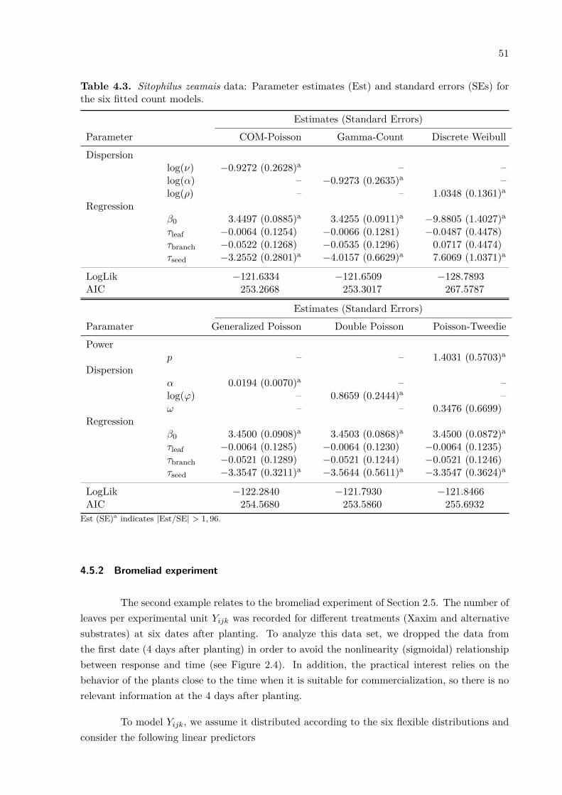
51
Table 4.3. Sitophilus zeamais data: Parameter estimates (Est) and standard errors (SEs) forthe six fitted count models.
Estimates (Standard Errors)Parameter COM-Poisson Gamma-Count Discrete WeibullDispersion
log(ν) −0.9272 (0.2628)a – –log(α) – −0.9273 (0.2635)a –log(ρ) – – 1.0348 (0.1361)a
Regressionβ0 3.4497 (0.0885)a 3.4255 (0.0911)a −9.8805 (1.4027)a
τleaf −0.0064 (0.1254) −0.0066 (0.1281) −0.0487 (0.4478)τbranch −0.0522 (0.1268) −0.0535 (0.1296) 0.0717 (0.4474)τseed −3.2552 (0.2801)a −4.0157 (0.6629)a 7.6069 (1.0371)a
LogLik −121.6334 −121.6509 −128.7893AIC 253.2668 253.3017 267.5787
Estimates (Standard Errors)Paramater Generalized Poisson Double Poisson Poisson-TweediePower
p – – 1.4031 (0.5703)a
Dispersionα 0.0194 (0.0070)a – –log(φ) – 0.8659 (0.2444)a –ω – – 0.3476 (0.6699)
Regressionβ0 3.4500 (0.0908)a 3.4503 (0.0868)a 3.4500 (0.0872)a
τleaf −0.0064 (0.1285) −0.0064 (0.1230) −0.0064 (0.1235)τbranch −0.0521 (0.1289) −0.0521 (0.1244) −0.0521 (0.1246)τseed −3.3547 (0.3211)a −3.5644 (0.5611)a −3.3547 (0.3624)a
LogLik −122.2840 −121.7930 −121.8466AIC 254.5680 253.5860 255.6932
Est (SE)a indicates |Est/SE| > 1, 96.
4.5.2 Bromeliad experiment
The second example relates to the bromeliad experiment of Section 2.5. The number ofleaves per experimental unit Yijk was recorded for different treatments (Xaxim and alternativesubstrates) at six dates after planting. To analyze this data set, we dropped the data fromthe first date (4 days after planting) in order to avoid the nonlinearity (sigmoidal) relationshipbetween response and time (see Figure 2.4). In addition, the practical interest relies on thebehavior of the plants close to the time when it is suitable for commercialization, so there is norelevant information at the 4 days after planting.
To model Yijk, we assume it distributed according to the six flexible distributions andconsider the following linear predictors
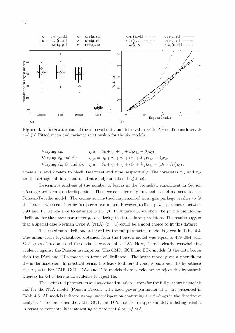
52
(a)
Num
ber
of e
mer
gent
inse
cts
0
10
20
30
40
Control Leaf Branch Seed
● ●●
●
● CMP(µi, ν)GCT(κi, α)DWe(qi, ρ)
GPo(µi, σ)DPo(µi, ϕ)PTwp(µi, ω)
(b)Expected value
Var
ianc
e
20
40
60
80
100
0 10 20 30
CMP(µi, ν)GCT(κi, α)DWe(qi, ρ)
GPo(µi, σ)DPo(µi, ϕ)PTwp(µi, ω)
Figure 4.4. (a) Scatterplots of the observed data and fitted values with 95% confidence intervalsand (b) Fitted mean and variance relationship for the six models.
Varying β0: ηijk = β0 + γi + τj + β1x1k + β2x2k
Varying β0 and β1: ηijk = β0 + γi + τj + (β1 + δ1j)x1k + β2x2k
Varying β0, β1 and β2: ηijk = β0 + γi + τj + (β1 + δ1j)x1k + (β2 + δ2j)x2k,
where i, j, and k refers to block, treatment and time, respectively. The covariates x1k and x2k
are the orthogonal linear and quadratic polynomials of log(time).Descriptive analysis of the number of leaves in the bromeliad experiment in Section
2.5 suggested strong underdispersion. Thus, we consider only first and second moments for thePoisson-Tweedie model. The estimation method implemented in mcglm package crashes to fitthis dataset when considering free power parameter. However, to fixed power parameter between0.93 and 1.1 we are able to estimate ω and β. In Figure 4.5, we show the profile pseudo-log-likelihood for the power parameter p, considering the three linear predictors. The results suggestthat a special case Neyman Type A (NTA) (p = 1) could be a good choice to fit this dataset.
The maximum likelihood achieved by the full parametric model is given in Table 4.4.The minus twice log-likelihood obtained from the Poisson model was equal to 439.4984 with82 degrees of fredoom and the deviance was equal to 1.82. Here, there is clearly overwhelmingevidence against the Poisson assumption. The CMP, GCT and DPo models fit the data betterthan the DWe and GPo models in terms of likelihood. The latter model gives a poor fit forthe underdispersion. In practical terms, this leads to different conclusions about the hypothesisH0: β1j = 0. For CMP, GCT, DWe and DPo models there is evidence to reject this hypothesiswhereas for GPo there is no evidence to reject H0.
The estimated parameters and associated standard errors for the full parametric modelsand for the NTA model (Poisson-Tweedie with fixed power parameter at 1) are presented inTable 4.5. All models indicate strong underdispersion confirming the findings in the descriptiveanalysis. Therefore, since the CMP, GCT, and DPo models are approximately indistinguishablein terms of moments, it is interesting to note that ν̂ ≈ 1/φ̂ ≈ α̂.
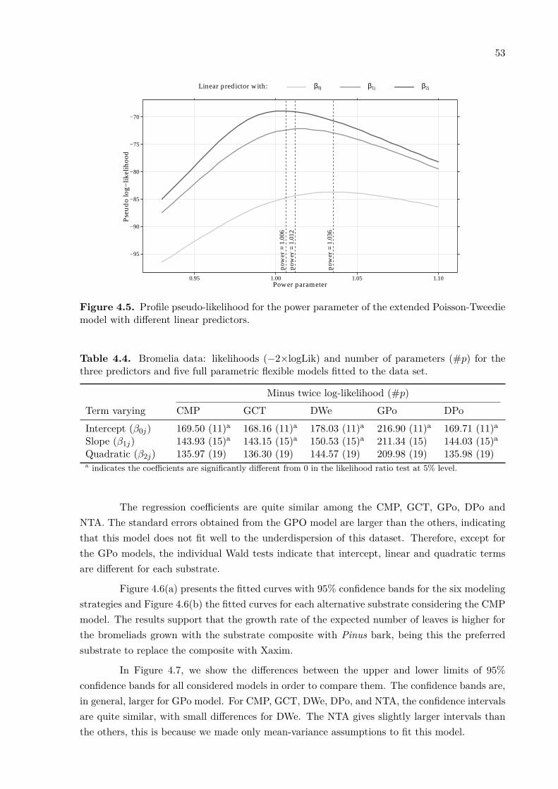
53
Power parameter
Pseu
do
log−
likel
ihoo
d
−95
−90
−85
−80
−75
−70
0.95 1.00 1.05 1.10
pow
er=
1.03
6
pow
er=
1.01
2po
wer
=1.
006
Linear predictor with: β0j β1j β2j
Figure 4.5. Profile pseudo-likelihood for the power parameter of the extended Poisson-Tweediemodel with different linear predictors.
Table 4.4. Bromelia data: likelihoods (−2×logLik) and number of parameters (#p) for thethree predictors and five full parametric flexible models fitted to the data set.
Minus twice log-likelihood (#p)
Term varying CMP GCT DWe GPo DPoIntercept (β0j) 169.50 (11)a 168.16 (11)a 178.03 (11)a 216.90 (11)a 169.71 (11)a
Slope (β1j) 143.93 (15)a 143.15 (15)a 150.53 (15)a 211.34 (15) 144.03 (15)a
Quadratic (β2j) 135.97 (19) 136.30 (19) 144.57 (19) 209.98 (19) 135.98 (19)a indicates the coefficients are significantly different from 0 in the likelihood ratio test at 5% level.
The regression coefficients are quite similar among the CMP, GCT, GPo, DPo andNTA. The standard errors obtained from the GPO model are larger than the others, indicatingthat this model does not fit well to the underdispersion of this dataset. Therefore, except forthe GPo models, the individual Wald tests indicate that intercept, linear and quadratic termsare different for each substrate.
Figure 4.6(a) presents the fitted curves with 95% confidence bands for the six modelingstrategies and Figure 4.6(b) the fitted curves for each alternative substrate considering the CMPmodel. The results support that the growth rate of the expected number of leaves is higher forthe bromeliads grown with the substrate composite with Pinus bark, being this the preferredsubstrate to replace the composite with Xaxim.
In Figure 4.7, we show the differences between the upper and lower limits of 95%confidence bands for all considered models in order to compare them. The confidence bands are,in general, larger for GPo model. For CMP, GCT, DWe, DPo, and NTA, the confidence intervalsare quite similar, with small differences for DWe. The NTA gives slightly larger intervals thanthe others, this is because we made only mean-variance assumptions to fit this model.

54
(a)Days after planting
Num
ber
of le
aves 10
15
Xaxim200 250 300 350 400
Pinus bark Eucalyptus bark
200 250 300 350 400
Coxim
10
15
Coconut fiber
CMP(µi, ν)GCT(κi, α)DWe(qi, ρ)
GPo(µi, σ)DPo(µi, ϕ)NTA(µi, ω)
(b)Days after planting
Num
ber
of le
aves
8
10
12
14
16
18
200 250 300 350 400
XaximPinus barkEucalyptus barkCoximCoconut fiber
Figure 4.6. (a) Scatterplots of the observed data and fitted values with 95% confidence bandsand (b) Fitted curves for each treatment considering the CMP model.
CMP1.0
1.51.0 1.5
0.5
1.0
0.5 1.0 ●●●
●●●●●●●●●●●●●●●
●●
●●●
●●●● ●●●●●●
●●●●●
●●
●●●
●●●●●
●●●●●●●● ●●
●●
●●
●●●●
●●●●●●●●●
●●●●●
●●
●●●●
●●●●●●●
●●●●●
●●
●●●●●●●●●
●●●●●●
●●●●●
GCT1.0
1.51.0 1.5
0.5
1.0
0.5 1.0 ●●●●●●● ●●●●●●
●●●●
● ●●
●●●●●●●●●●●●●
●●● ●● ●●
●●●●●●●●●
●●●●●●
●●●●●
●●●●●●●●●
●●●●●●
●●●●●
●
●●●●●
●
●●●●●●
●●●●●
●●
●
●●●●●
●
●●●●●
●●●●●●
●●
DWe1.0
1.51.0 1.5
0.5
1.0
0.5 1.0●
●●●●●
●
●●
●●●●
●●● ●●
●●
●
●●●●●
●
●●●●●●
●●●●●
●●
●
●●●●●
●
●●●●●●
●●●●●
●●
●●●●
●●●●
●●●●●
●●●
●●
●●
●●●●
●●●●
●●●●●
●●●
●●
●●
● ●●●
●●● ●
●●
●●●
●● ●
●●
●● GPo1.0
1.51.0 1.5
0.5
1.0
0.5 1.0
●●●●
●●●●
●●●●●
●●●
●●
●●
●●●●
●●●●
●●●●●
●●●
●●
●●
●●
●●●●
●●●●●●●●●
●●●●●
●●●
●●●●●●●●●●●●●●●
●●
●●●
●●●● ●●●●●●
●●●●●
●●
●●●
●●●●●
●●●●●●●● ●●
●●DPo1.0
1.51.0 1.5
0.5
1.0
0.5 1.0 ●●
●●●●
●●●●●●●
●●●●●
●●
●●●●●●●●●●●●●●●
●●●●●
●●●●●●●●●●●●●●●●●●
●●
● ●●●●●● ●●●●●●
●●●●●
●●
●●●●●●●●
●●●●●●●● ●●
●●
●●●●●●●●●●●●●●●
●●●●●
NTA1.0
1.51.0 1.5
0.5
1.0
0.5 1.0
µ̂ijk
● XaximPinus barkEucalyptus barkCoximCoconut fiber
810121416
Figure 4.7. Pairwise plot of the differences between the upper and lower limits of 95% confi-dence bands for all considered models. Symbols refer to the treatments and colors refer to thefitted values.
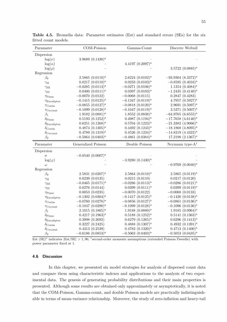
55
Table 4.5. Bromelia data: Parameter estimates (Est) and standard errors (SEs) for the sixfitted count models.
Paramater COM-Poisson Gamma-Count Discrete WeibullDispersion
log(ν) 3.9689 (0.1430)a – –log(α) – 4.4197 (0.2097)a
log(ρ) – – 3.5722 (0.0885)a
Regressionβ0 2.5865 (0.0110)a 2.6224 (0.0102)a −93.9304 (8.3372)a
γII 0.0217 (0.0110)a 0.0233 (0.0103)a −0.8595 (0.4016)a
γIII −0.0285 (0.0113)a −0.0271 (0.0106)a 1.1354 (0.4084)a
γIV 0.0400 (0.0111)a 0.0397 (0.0103)a −1.2435 (0.4140)a
τPinus −0.0070 (0.0122) −0.0068 (0.0115) 0.2847 (0.4283)τEucaliptos −0.1415 (0.0125)a −0.1347 (0.0119)a 4.7957 (0.5927)a
τCoxim −0.0855 (0.0127)a −0.0818 (0.0120)a 2.9691 (0.5097)a
τCoconut −0.1099 (0.0128)a −0.1047 (0.0119)a 3.5371 (0.5007)a
β1 1.9182 (0.0881)a 1.8552 (0.0838)a −64.9765 (6.6555)a
δPinus 0.5193 (0.1252)a 0.4987 (0.1194)a −17.7658 (4.6140)a
δEucaliptos 0.6251 (0.1268)a 0.5704 (0.1223)a −21.3382 (4.9066)a
δCoxim 0.4874 (0.1305)a 0.4492 (0.1243)a −18.1868 (4.8095)a
δCoconut 0.4789 (0.1319)a 0.4526 (0.1234)a −14.8219 (4.4322)a
β2 −0.5064 (0.0403)a −0.4861 (0.0384)a 17.2198 (2.1367)a
Paramater Generalized Poisson Double Poisson Neymann type-A1
Dispersionσ −0.0540 (0.0007)a – –log(φ) – −3.9280 (0.1430)a –ω – – −0.9769 (0.0040)a
Regressionβ0 2.5831 (0.0207)a 2.5864 (0.0110)a 2.5865 (0.0119)a
γII 0.0239 (0.0135) 0.0215 (0.0110) 0.0217 (0.0120)γIII −0.0465 (0.0171)a −0.0286 (0.0113)a −0.0286 (0.0121)a
γIV 0.0276 (0.0144) 0.0399 (0.0111)a 0.0399 (0.0119)a
τPinus 0.0053 (0.0235) −0.0070 (0.0122) −0.0068 (0.0133)τEucaliptos −0.1302 (0.0304)a −0.1417 (0.0125)a −0.1420 (0.0138)a
τCoxim −0.0760 (0.0276)a −0.0856 (0.0127)a −0.0861 (0.0136)a
τCoconut −0.1047 (0.0290)a −0.1099 (0.0128)a −0.1096 (0.0136)a
β1 2.1015 (0.1865)a 1.9188 (0.0880)a 1.9185 (0.0964)a
δPinus 0.4217 (0.1963)a 0.5188 (0.1252)a 0.5141 (0.1363)a
δEucaliptos 0.3998 (0.2692) 0.6279 (0.1265)a 0.6296 (0.1413)a
δCoxim 0.3227 (0.2425) 0.4888 (0.1307)a 0.4932 (0.1391)a
δCoconut 0.4313 (0.2539) 0.4783 (0.1320)a 0.4713 (0.1400)a
β2 −0.6186 (0.0853)a −0.5063 (0.0403)a −0.5053 (0.0435)a
Est (SE)a indicates |Est/SE| > 1, 96; 1second-order moments assumptions (extended Poisson-Tweedie) withpower parameter fixed at 1.
4.6 Discussion
In this chapter, we presented six model strategies for analysis of dispersed count dataand compare them using characteristic indexes and applications to the analysis of two exper-imental data. The genesis of generating probability distributions and their main properties ispresented. Although some results are obtained only approximately or asymptotically, it is notedthat the COM-Poisson, Gamma-count, and double Poisson models are practically indistinguish-able in terms of mean-variance relationship. Moreover, the study of zero-inflation and heavy-tail
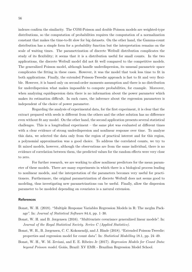
56
indexes confirm the similarity. The COM-Poisson and double Poisson models are weighted-typedistributions, so the computation of probabilities requires the computation of a normalizationconstant that makes the time-to-fit slow for big datasets. On the other hand, the Gamma-countdistribution has a simple form for a probability function but the interpretation remains on thescale of waiting times. The parametrization of discrete Weibull distribution complicates thestudy of its flexibility; it seems that it is a distribution useful for small counts. In the twoapplications, the discrete Weibull model did not fit well compared to the competitive models.The generalized Poisson model, although handle underdispersion, its unusual parametric spacecomplicates the fitting in these cases. However, it was the model that took less time to fit inboth applications. Finally, the extended Poisson-Tweedie approach is fast to fit and very flexi-ble. However, it is based only on second-order moments assumption and there is no distributionfor underdispersion what makes impossible to compute probabilities, for example. Moreover,when analyzing equidispersion data there is no information about the power parameter whichmakes its estimation difficult. In such cases, the inference about the regression parameters isindependent of the choice of power parameter.
Regarding the analysis of experimental data, for the first experiment, it is clear that theextract prepared with seeds is different from the others and the other solution has no differenceeven without fit any model. On the other hand, the second application presents several statisticalchallenges. This is a longitudinal experiment – the same plot was evaluated at different timeswith a clear evidence of strong underdispersion and nonlinear response over time. To analyzethis data, we selected the data only from the region of practical interest and for this region,a polynomial approximation was a good choice. To address the correlated counts, we try tofit mixed models, however, although the observations are from the same individual, there is noevidence of correlation between them, the predicted values for the random effects were very closeto zero.
For further research, we are working to allow nonlinear predictors for the mean param-eter of these models. There are many experiments in which there is a biological process leadingto nonlinear models, and the interpretation of the parameters becomes very useful for practi-tioners. Furthermore, the original parametrization of discrete Weibull does not seems good tomodeling, thus investigating new parametrizations can be useful. Finally, allow the dispersionparameter to be modeled depending on covariates is a natural extension.
References References
Bonat, W. H. (2018). “Multiple Response Variables Regression Models in R: The mcglm Pack-age”. In: Journal of Statistical Software 84.4, pp. 1–30.
Bonat, W. H. and B. Jørgensen (2016). “Multivariate covariance generalized linear models”. In:Journal of the Royal Statistical Society. Series C (Applied Statistics).
Bonat, W. H., B. Jørgensen, C. C. Kokonendji, and J. Hinde (2018). “Extended Poisson-Tweedie:properties and regression model for count data”. In: Statistical Modelling 18.1, pp. 24–49.
Bonat, W. H., W. M. Zeviani, and E. E. Ribeiro Jr (2017). Regression Models for Count Data:beyond Poisson model. Goiás, Brazil: XV EMR - Brazilian Regression Model School.
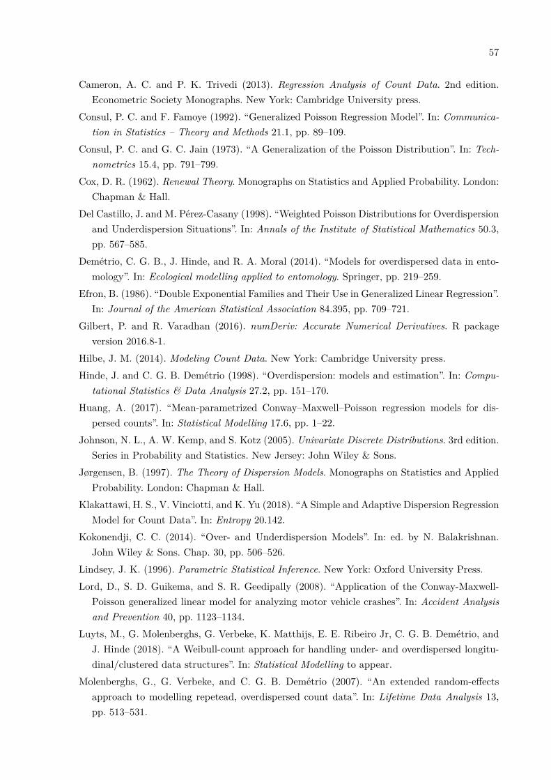
57
Cameron, A. C. and P. K. Trivedi (2013). Regression Analysis of Count Data. 2nd edition.Econometric Society Monographs. New York: Cambridge University press.
Consul, P. C. and F. Famoye (1992). “Generalized Poisson Regression Model”. In: Communica-tion in Statistics – Theory and Methods 21.1, pp. 89–109.
Consul, P. C. and G. C. Jain (1973). “A Generalization of the Poisson Distribution”. In: Tech-nometrics 15.4, pp. 791–799.
Cox, D. R. (1962). Renewal Theory. Monographs on Statistics and Applied Probability. London:Chapman & Hall.
Del Castillo, J. and M. Pérez-Casany (1998). “Weighted Poisson Distributions for Overdispersionand Underdispersion Situations”. In: Annals of the Institute of Statistical Mathematics 50.3,pp. 567–585.
Demétrio, C. G. B., J. Hinde, and R. A. Moral (2014). “Models for overdispersed data in ento-mology”. In: Ecological modelling applied to entomology. Springer, pp. 219–259.
Efron, B. (1986). “Double Exponential Families and Their Use in Generalized Linear Regression”.In: Journal of the American Statistical Association 84.395, pp. 709–721.
Gilbert, P. and R. Varadhan (2016). numDeriv: Accurate Numerical Derivatives. R packageversion 2016.8-1.
Hilbe, J. M. (2014). Modeling Count Data. New York: Cambridge University press.Hinde, J. and C. G. B. Demétrio (1998). “Overdispersion: models and estimation”. In: Compu-
tational Statistics & Data Analysis 27.2, pp. 151–170.Huang, A. (2017). “Mean-parametrized Conway–Maxwell–Poisson regression models for dis-
persed counts”. In: Statistical Modelling 17.6, pp. 1–22.Johnson, N. L., A. W. Kemp, and S. Kotz (2005). Univariate Discrete Distributions. 3rd edition.
Series in Probability and Statistics. New Jersey: John Wiley & Sons.Jørgensen, B. (1997). The Theory of Dispersion Models. Monographs on Statistics and Applied
Probability. London: Chapman & Hall.Klakattawi, H. S., V. Vinciotti, and K. Yu (2018). “A Simple and Adaptive Dispersion Regression
Model for Count Data”. In: Entropy 20.142.Kokonendji, C. C. (2014). “Over- and Underdispersion Models”. In: ed. by N. Balakrishnan.
John Wiley & Sons. Chap. 30, pp. 506–526.Lindsey, J. K. (1996). Parametric Statistical Inference. New York: Oxford University Press.Lord, D., S. D. Guikema, and S. R. Geedipally (2008). “Application of the Conway-Maxwell-
Poisson generalized linear model for analyzing motor vehicle crashes”. In: Accident Analysisand Prevention 40, pp. 1123–1134.
Luyts, M., G. Molenberghs, G. Verbeke, K. Matthijs, E. E. Ribeiro Jr, C. G. B. Demétrio, andJ. Hinde (2018). “A Weibull-count approach for handling under- and overdispersed longitu-dinal/clustered data structures”. In: Statistical Modelling to appear.
Molenberghs, G., G. Verbeke, and C. G. B. Demétrio (2007). “An extended random-effectsapproach to modelling repetead, overdispersed count data”. In: Lifetime Data Analysis 13,pp. 513–531.
58
Nakagawa, T. and S. Osaki (1975). “The Discrete Weibull Distribution”. In: IEEE Transactionson Reliability 24.5, pp. 300–301.
Puig, P. and J. Valero (2006). “Count data distributions: some characterizations with applica-tions”. In: Journal of the American Statistical Association 101.473, pp. 332–340.
R Core Team (2018). R: A Language and Environment for Statistical Computing. R Foundationfor Statistical Computing. Vienna, Austria.
Ribeiro Jr, E. E., W. M. Zeviani, W. H. Bonat, C. G. B. Demétrio, and J. Hinde (2018).“Reparametrization of COM-Poisson Regression Models with Applications in the Analysis ofExperimental Data”. In: arXiv (Statistics Applications and Statistics Methodology).
Rigby, R. A. and D. M. Stasinopoulos (2005). “Generalized additive models for location, scaleand shape (with discussion)”. In: Journal of the Royal Statistical Society. Series C (AppliedStatistics) 54.3, pp. 507–554.
Sellers, K. F. and D. S. Morris (2017). “Underdispersion models: Models that are “under theradar””. In: Communication in Statistics – Theory and Methods 46.24, pp. 12075–12086.
Sellers, K. F. and G. Shmueli (2010). “A flexible regression model for count data”. In: Annals ofApplied Statistics 4.2, pp. 943–961.
Shmueli, G., T. P. Minka, J. B. Kadane, S. Borle, and P. Boatwright (2005). “A useful dis-tribution for fitting discrete data: Revival of the Conway-Maxwell-Poisson distribution”. In:Journal of the Royal Statistical Society. Series C (Applied Statistics) 54.1, pp. 127–142.
Wedderburn, R. W. M. (1974). “Quasi-Likelihood Functions, Generalized Linear Models, andthe Gauss-Newton Method”. In: Biometrika 61.3, p. 439.
Winkelmann, R. (1995). “Duration Dependence and Dispersion in Count-Data Models”. In:Journal of Business & Economic Statistics 13.4, pp. 467–474.
Winkelmann, R. (2008). Econometric Analysis of Count Data. 5th edition. Berlin, Heidelberg:Springer-Velag, p. 342.
Zamani, H. and N. Ismail (2012). “Functional Form for the Generalized Poisson RegressionModel”. In: Communication in Statistics – Theory and Methods 41, pp. 3666–3675.
Zeviani, W. M., P. J. Ribeiro Jr, W. H. Bonat, S. E. Shimakura, and J. A. Muniz (2014). “TheGamma-count distribution in the analysis of experimental underdispersed data”. In: Journalof Applied Statistics 41.12, pp. 2616–2626.
Zou, Y., S. R. Geedipally, and D. Lord (2013). “Evaluating the double Poisson generalized linearmodel”. In: Accident Analysis and Prevention 59, pp. 497–505.
59
5 COM-POISSON MODELS WITH VARYING DISPERSION
ABSTRACTThere are many experiments that experimental conditions can have an effect on mean and
dispersion. In this case, models with constant dispersion can produce a loss of efficiency.In this chapter, we propose an extension of the COM-Poisson model to jointly model themean and the dispersion. This approach allows analyzing the data that exhibit under-and overdispersion depending on covariates. The estimation and inference are based onlikelihood method. We carried out simulation studies to verify the finite sample propertiesof the maximum likelihood estimators. The results from our simulation study show that themaximum likelihood estimators are unbiased and consistent for both mean and dispersionregression parameters. The application of the COM-Poisson models with varying dispersionis illustrated with the analysis of two experimental datasets. The computational routines forfitting the models and the datasets are available in the appendix.
Keywords: COM-Poisson distribution, Double generalized linear models, GAMLSS, Vary-ing dispersion.
5.1 Introduction
The standard Gaussian linear models are based on the assumption of variance ho-mogeneity (Aitkin 1987). Generalized linear models relax this assumption by assuming theobservations come from some distribution in the exponential family (Nelder and Wedderburn1972). A key feature of exponential family distribution is the so-called mean-variance relation-ship, i.e. the variance is a deterministic function of the mean Var(Y ) = ϕV (µ). The mainexamples are V (µ) = µ(1 − µ) for the binomial distribution, V (µ) = µ for the Poisson distribu-tion, V (µ) = µ2 for the gamma distribution and V (µ) = µ3 for the inverse-Gaussian distribution(McCullagh and Nelder 1989). This allows modeling specific heterogeneity by assuming an ap-propriate distribution. However, once the mean-variance relationship is specified, the varianceis assumed to be known up to a constant of proportionality, the dispersion parameter~ϕ. Toensure more flexibility in the analysis of non-Gaussian heterogeneous data, we explore methodsto model dispersion depending on covariates. We focus on count data only.
Modeling dispersion depending on covariates in the analysis of count data has not beenmuch explored in the literature. The class of double generalized linear models (Smyth 1988;McCullagh and Nelder 1989; Smyth and Verbyla 1999) can be used to do it. This class waswidely explored for continuous data. Smyth (1988) discussed this class using a double generalizedlinear model based on the gamma distribution. Adjusted likelihood methods for estimationand inference are presented by Smyth and Verbyla (1999). Paula (2013) discussed diagnosticsfor this class and used a assumed gamma distributed data as an application. Andersen andBonat (2017) extended the double generalized linear model by considering compound Poissondistributions. Related to discrete data, Vieira et al. (2011) proposed a Bayesian analysis of thedouble generalized linear models for binomial data.
Another approach that has gained momentum in the last decade is the generalizedadditive models for location, shape, and scale (GAMLSS) (Rigby and Stasinopoulos 2005). This
60
approach extends the generalized linear models in different directions: (i) the distribution forthe response variable can be selected from a more general family; the only restriction is that thederivatives with respect to each parameter must be computable, (ii) all parameters of the distri-bution can be depended on covariates, and (iii) the systematic relationship between covariatesand parameters can be parametric (linear predictor) or nonparametric (smooth) functions.
In this chapter, we propose to jointly model the mean and dispersion based on theCOM-Poisson distribution. This approach is very similar to the GAMLSS, however, we de-velop and explore our own estimation methods. This approach allows data exhibit under- andoverdispersion depending on experimental conditions.
This chapter is organized as follows. In Section 5.2, we briefly describe and discuss thedouble generalized linear models. The newly proposed COM-Poisson models is considered inSection 5.3. In Section 5.4, we present estimation and inference for the COM-Poisson regressionmodel in a likelihood framework. Section 5.6 is devoted to illustrate the application of theCOM-Poisson model with varying dispersion for the analysis of two data sets. We compare theresults of COM-Poisson model with double generalized linear models and GAMLSS approach.Finally, concluding remarks close the chapter in Section 5.7. We provide an R implementationfor fitting the COM-Poisson models with varying dispersion, together with the analyzed datasets, ins the package cmpreg. Illustrative codes are presented in the appendix.
5.2 Double generalized linear models
Following Smyth (1988) and McCullagh and Nelder (1989, chap. 10), the so-calleddouble generalized linear models (DGLM) can be used to model mean and dispersion jointlyby considering two linked generalized linear models (GLM). Let yi, i = 1, 2, . . . , n be a set ofindependent observations of Yi and xi = (xi1, xi2, . . . , xnp)⊤ a vector of known covariates. Thestandard GLMs assume that
E(Yi) = µi, g(µi) = ηi = x⊤i β and Var(Yi) = ϕV (µi),
where g(.) is a suitable link function and V (.) is the variance function. The DGLMs generalizethe GLMs to allow the dispersion parameter varying across observations, Var(Yi) = ϕiV (µi).The model for dispersion is specified by
E(di) = ϕi, h(ϕi) = ξi = z⊤i γ and Var(di) = τVd(ϕi),
where di is a suitable statistic chosen as a measure of dispersion, h(.) is the dispersion linkfunction and Vd(.) is the dispersion variance function. The commom choice for di is the deviancecomponents from the mean model. Based on asymptotic distribution of di, a gamma model withVd(ϕi) = 2ϕ2
i is a suitable natural choice for the dispersion model.The parameter estimation proposed is based on a two-step iterative algorithm: (i)
holding γ fixed we obtain the dispersion components and estimate β; and (ii) fixing the estimatedvalue of β, we obtain the deviance components and estimate γ. These two steps are thenalternated until convergence.
The idea of using a interlinked pair of generalized linear models for allowing mean anddispersion effects depend on covariates was first put forward by Pregibon (1984) and further
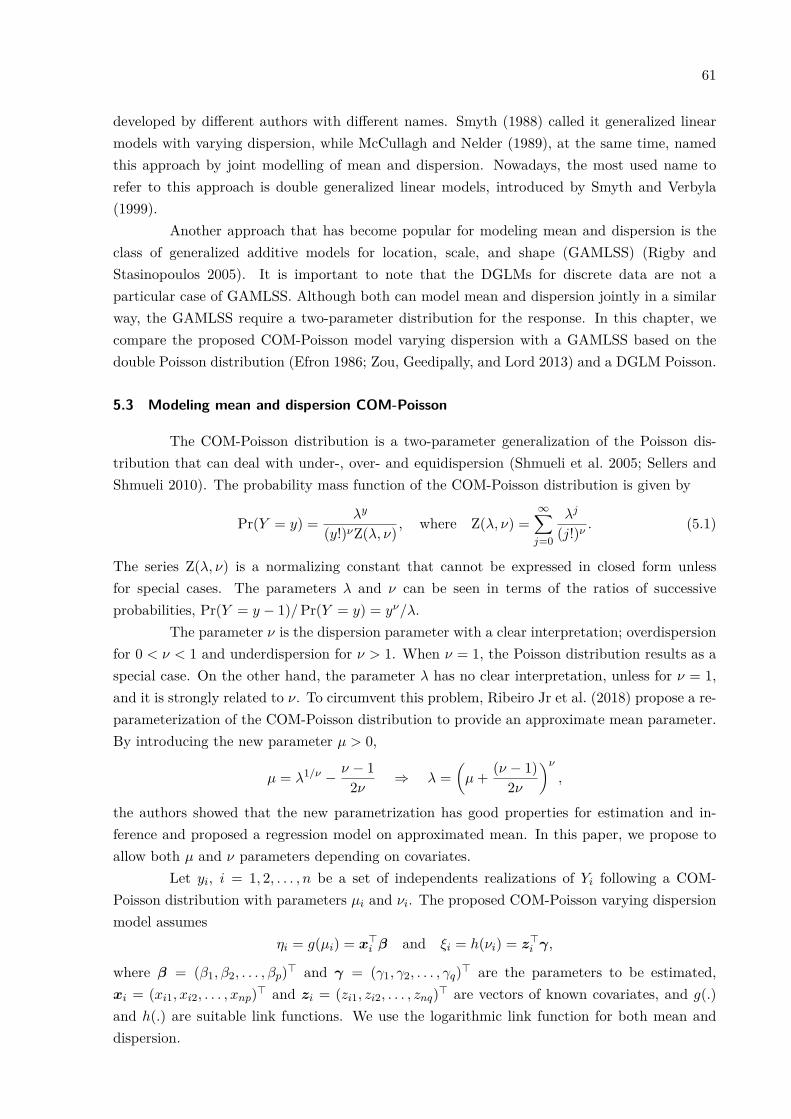
61
developed by different authors with different names. Smyth (1988) called it generalized linearmodels with varying dispersion, while McCullagh and Nelder (1989), at the same time, namedthis approach by joint modelling of mean and dispersion. Nowadays, the most used name torefer to this approach is double generalized linear models, introduced by Smyth and Verbyla(1999).
Another approach that has become popular for modeling mean and dispersion is theclass of generalized additive models for location, scale, and shape (GAMLSS) (Rigby andStasinopoulos 2005). It is important to note that the DGLMs for discrete data are not aparticular case of GAMLSS. Although both can model mean and dispersion jointly in a similarway, the GAMLSS require a two-parameter distribution for the response. In this chapter, wecompare the proposed COM-Poisson model varying dispersion with a GAMLSS based on thedouble Poisson distribution (Efron 1986; Zou, Geedipally, and Lord 2013) and a DGLM Poisson.
5.3 Modeling mean and dispersion COM-Poisson
The COM-Poisson distribution is a two-parameter generalization of the Poisson dis-tribution that can deal with under-, over- and equidispersion (Shmueli et al. 2005; Sellers andShmueli 2010). The probability mass function of the COM-Poisson distribution is given by
Pr(Y = y) = λy
(y!)νZ(λ, ν), where Z(λ, ν) =
∞∑j=0
λj
(j!)ν. (5.1)
The series Z(λ, ν) is a normalizing constant that cannot be expressed in closed form unlessfor special cases. The parameters λ and ν can be seen in terms of the ratios of successiveprobabilities, Pr(Y = y − 1)/Pr(Y = y) = yν/λ.
The parameter ν is the dispersion parameter with a clear interpretation; overdispersionfor 0 < ν < 1 and underdispersion for ν > 1. When ν = 1, the Poisson distribution results as aspecial case. On the other hand, the parameter λ has no clear interpretation, unless for ν = 1,and it is strongly related to ν. To circumvent this problem, Ribeiro Jr et al. (2018) propose a re-parameterization of the COM-Poisson distribution to provide an approximate mean parameter.By introducing the new parameter µ > 0,
µ = λ1/ν − ν − 12ν
⇒ λ =(µ+ (ν − 1)
2ν
)ν
,
the authors showed that the new parametrization has good properties for estimation and in-ference and proposed a regression model on approximated mean. In this paper, we propose toallow both µ and ν parameters depending on covariates.
Let yi, i = 1, 2, . . . , n be a set of independents realizations of Yi following a COM-Poisson distribution with parameters µi and νi. The proposed COM-Poisson varying dispersionmodel assumes
ηi = g(µi) = x⊤i β and ξi = h(νi) = z⊤
i γ,
where β = (β1, β2, . . . , βp)⊤ and γ = (γ1, γ2, . . . , γq)⊤ are the parameters to be estimated,xi = (xi1, xi2, . . . , xnp)⊤ and zi = (zi1, zi2, . . . , znq)⊤ are vectors of known covariates, and g(.)and h(.) are suitable link functions. We use the logarithmic link function for both mean anddispersion.

62
The COM-Poisson model with varying dispersion is quite similar to the double general-ized linear approach, both extend the generalized linear models to model the dispersion as wellas the mean. However, COM-Poisson with varying dispersion is a fully parametric model thathas the advantages of allowing predictions for probabilities and generalizations such as randomeffects and modeling of censored data.
5.4 Estimation and inference
To fit COM-Poisson models with varying dispersion, we use the maximum likelihoodestimation method. The log-likelihood function for θ = (β⊤,γ⊤)⊤ parameters is given by
ℓ = ℓ(θ; y) =n∑
i=1
{νi log
(µi + νi − 1
2νi
)− νi log(yi) − log[Z(µi, νi)]
}, (5.2)
where µi = exp(x⊤i β), νi = exp(z⊤
i γ), and Z(µi, νi) is a normalizing constant computed for theparameters µi and νi.
Parameter estimation requires the numerical maximization of Equation (5.2). Since thederivatives of ℓ cannot be obtained in closed forms, we compute them by central finite differencesusing the Richardson method as implemented in package numDeriv (Gilbert and Varadhan 2016)for the statistical software R (R Core Team 2018). Based on the orthogonality property betweenµi and νi (see Ribeiro Jr et al. 2018), we set two strategies to obtain the maximum likelihoodestimates:
(a) the joint strategy, where we obtain β̂ and γ̂ jointly by maximizing ℓ(θ; y); and
(b) the two-stages strategy, where we fix β̂ at the maximum likelihood estimates of Poissonmodel and obtain γ̂ by maximizing ℓ(γ; β = β̂,y) and then estimate the Hessian matrixat (β̂, γ̂).
Although we have an additional step for estimating the Hessian matrix, the strategy(b) tends to be faster than (a), because of the maximization is performed in Rq whereas, forstrategy (a), the estimation is an optimization problem in Rp+q space.
Standard errors for the parameter estimates are obtained based on the observed infor-mation matrix. Let the derivatives be computed at the maximum likelihood estimates. Thevariance and covariance matrix of the maximum likelihood estimators may be expressed as
Vθ =(
−∂ℓ2/∂β∂β⊤ −∂ℓ2/∂β∂γ⊤
−∂ℓ2/∂γ∂β⊤ −∂ℓ2/∂γ∂γ⊤
)−1
=(
Vβ Vβγ
Vγβ Vγ
).
Based on the asymptotic distribution of the maximum likelihood estimators, we obtainthe variances for η̂i and ξ̂i using delta method, Var(η̂i) = x⊤
i Vβ|γxi and Var(ξ̂i) = z⊤i Vγ|βzi,
where Vβ|γ = Vβ − VβγV −1γ Vγβ and Vγ|β = Vγ − VγβV −1
β Vβγ . Since β and γ were found to benearly orthogonal, Vβγ = V ⊤
γβ ≈ 0, hence Vβ|γ ≈ Vβ and Vγ|β ≈ Vγ , in other words, inferencebased on the conditional log-likelihood and inference based on the marginal log-likelihood is thesame.
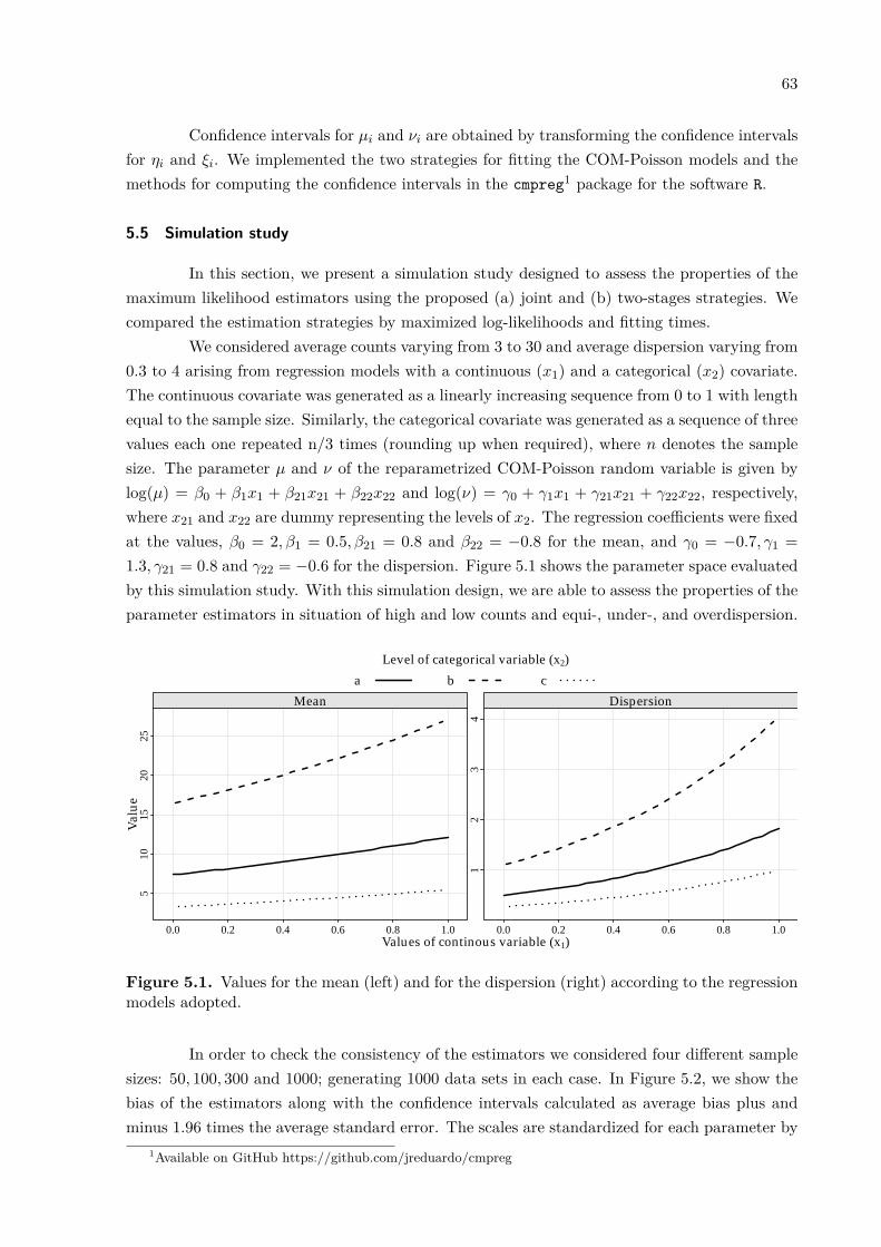
63
Confidence intervals for µi and νi are obtained by transforming the confidence intervalsfor ηi and ξi. We implemented the two strategies for fitting the COM-Poisson models and themethods for computing the confidence intervals in the cmpreg1 package for the software R.
5.5 Simulation study
In this section, we present a simulation study designed to assess the properties of themaximum likelihood estimators using the proposed (a) joint and (b) two-stages strategies. Wecompared the estimation strategies by maximized log-likelihoods and fitting times.
We considered average counts varying from 3 to 30 and average dispersion varying from0.3 to 4 arising from regression models with a continuous (x1) and a categorical (x2) covariate.The continuous covariate was generated as a linearly increasing sequence from 0 to 1 with lengthequal to the sample size. Similarly, the categorical covariate was generated as a sequence of threevalues each one repeated n/3 times (rounding up when required), where n denotes the samplesize. The parameter µ and ν of the reparametrized COM-Poisson random variable is given bylog(µ) = β0 + β1x1 + β21x21 + β22x22 and log(ν) = γ0 + γ1x1 + γ21x21 + γ22x22, respectively,where x21 and x22 are dummy representing the levels of x2. The regression coefficients were fixedat the values, β0 = 2, β1 = 0.5, β21 = 0.8 and β22 = −0.8 for the mean, and γ0 = −0.7, γ1 =1.3, γ21 = 0.8 and γ22 = −0.6 for the dispersion. Figure 5.1 shows the parameter space evaluatedby this simulation study. With this simulation design, we are able to assess the properties of theparameter estimators in situation of high and low counts and equi-, under-, and overdispersion.
Values of continous variable (x1)
Val
ue5
1015
2025
0.0 0.2 0.4 0.6 0.8 1.0
Mean
12
34
0.0 0.2 0.4 0.6 0.8 1.0
Dispersion
Level of categorical variable (x2)
a b c
Figure 5.1. Values for the mean (left) and for the dispersion (right) according to the regressionmodels adopted.
In order to check the consistency of the estimators we considered four different samplesizes: 50, 100, 300 and 1000; generating 1000 data sets in each case. In Figure 5.2, we show thebias of the estimators along with the confidence intervals calculated as average bias plus andminus 1.96 times the average standard error. The scales are standardized for each parameter by
1Available on GitHub https://github.com/jreduardo/cmpreg
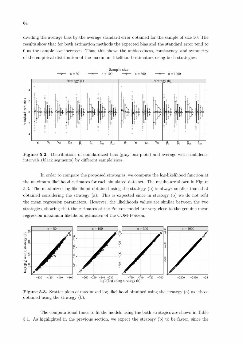
64
dividing the average bias by the average standard error obtained for the sample of size 50. Theresults show that for both estimation methods the expected bias and the standard error tend to0 as the sample size increases. Thus, this shows the unbiasedness, consistency, and symmetryof the empirical distribution of the maximum likelihood estimators using both strategies.
Stan
dar
diz
ed B
ias
−4
−2
0
2
4
γ0 γ1 γ21 γ22 β0 β1 β21 β22
●
●
●
●
●
●
●●
●
●●
●
●
●●
●
●
●
●
●
●
●●
●●
●
●
●●
●●
●
●
●
●
●●
●
●●
●
●
●
●
●
●●●●●
●
●
●
●●
●
●
●
●
●●
●
●●●
●
●
●
●
●
●
●
●
●
●
●
●
●●●
●
●●
●
●
●
●●
●
●●
●
●●●
●
●
●●
●●
●
●
●●●
●
●
●
●●●
●●
●●
●●
●
●
●
●
●
●
●
●
●
●●●
●
●
●
●
●
●
●
●●
●
●
●
●●●
●
●
●
●
●●
●●●
●●
●
●●● ●
●
●
●
●
●
●
●●●●
●●
●●
●
●●
●●●
●
●
●
●
●●
●●
●
●●
●
●●
●●●
●● ●●
●
●●
●
●
●
●
●
●●●
●
●
●
●
●●●
●
●
●●
●●●
●●●●
●
●●
●
●
●●
●●●●● ●●
●●
● ●●
●
●●
●
●
● ●
●●●
●●
●●
●
●
●
●
●●
●●
●
●●●
●
●● ● ● ● ● ● ●
Strategy (a)
γ0 γ1 γ21 γ22 β0 β1 β21 β22
●
●●
●
●
●●
●
●
●
●
●
●
●
●
●
●
●
●
●
●
●
●●
●
●
●●
●●
●
●
●
●
●
●
●
●
●
●●
●
●
●
●●
●
●
●
●
●
●
●
●
●
●
●
●●●
●
●
●
●
●
●●
●
●
●●
●●
●
●
●
●
●
●
●●
●
●
●
●
●●
●●
●
●
●
●
●●
●
●●●
●
●
●
●
●
●
●
●
●●
●●
●
●
●
●●●
●●
●
●●
●●
●
●
●●
●
●
●
●
●
●
●
●
●●●
●
●
●
●
●●
●
●
●
●●
●
●●●
●●
●
●●
●●●
●
●
●●●●
●●
●
●
●
●
●
●●●
●
●
●
●●
●● ●●
●●
●
●●
●●
●
●
●
●●
●
●
●● ●●●
●
●●
●
●
●
●
●●
●●●
●
●
●
●
●
●●●
●
●
●●
●●●
●●●●
●
●●●
●●
●●●●● ●
●
●●
●●
●
●
●
●
●
●●● ●
●●
●
●
●●
●
●●
●●
●
●
●
●
●●
●●
●●
●●●
●
●●
●
●
●● ● ● ● ● ●
Strategy (b)
Sample size● n = 50 n = 100 n = 300 n = 1000
Figure 5.2. Distributions of standardized bias (gray box-plots) and average with confidenceintervals (black segments) by different sample sizes.
In order to compare the proposed strategies, we compute the log-likelihood function atthe maximum likelihood estimates for each simulated data set. The results are shown in Figure5.3. The maximized log-likelihood obtained using the strategy (b) is always smaller than thatobtained considering the strategy (a). This is expected since in strategy (b) we do not refitthe mean regression parameters. However, the likelihoods values are similar between the twostrategies, showing that the estimates of the Poisson model are very close to the genuine meanregression maximum likelihood estimates of the COM-Poisson.
logL(β,γ) using strategy (b)
logL
(β,γ
) usi
ng s
trat
egy
(a)
−13
0−
120
−11
0−
100
−130 −120 −110 −100
●●
●
●
●
●
●
●●●
●●●
●
●
●
●
●●
●
●
●
●
●
●
●●
●
●
●
●
●
●
●
●
●●
●
●
●
●
●
●
●
●●
●
●
●
●
●
●
●
●●
●
●
●●
●
●
●●
●●
●
●●
●
●●
●
●
●●
●
●
●
●●
●
●
●
●
●
●
●
●
●●
●
●
●
●
●
●
●
●
●
●
●
●
●
●
●
●
●
●
●
●
●●
●
●●●
●●
●
●
●
●
●
●●
●●
●
●
●
●
●
●
●
●
●
●●
●
●
●
●
●●
●
●
●
●
●
●
●●
●●
●
●
●
●
●
●
●
●
●●●
●
●●
●
●●●
●
●
●
●
●
●
●
●●
●
●
●
●
● ●
●
●
●
●
●
●
●●
●
●
●●
●
●
●
●●
●
●
●
●
●
●
●
●
●
●
●
●
●
●
●
●
●
●
●
●●
●
●
●
●
●●
●
●●●●
●
●
●
●
●
●
●
●●
●
●
●
●
●
●●
●
●
●
●
●
●●
●
●
●
●●
●
●
●●
●
●
●
●
●
●
●
●
●
●●
●
●
●
●
●
●●
●
●
●
●
●●
●
●
●
●●
●
●
●
●
●●
●
●
●
●
●
●
●●
●
●
●
●
●
●
●●
●
●
●
●
●
●
●●
●
●
●
●
●●
●
●
●
●
●
●
●
●
●
●
●
●●
●
●●●
●
●
●●
●
●
●
●
●
●●
●●
●
●
●
●
●●
●
●
●
●●●
●
●
●
●●
●
●
●
●●
●
●
●
●
●●
●
●●●
●
●
●●
●
●
●
●●
●●
●
●
●
●
●
●
●
●
●
●
●
●
●
●
●
●
●
●
●
●
●
●●●
●
●
●●
●
●
●
●
●●
●
●
●
●
●
●
●
●
●
●
●
●
●
●
●
●
●●●
●
●
●●
●
●
●
●
●
●
●
●
●
●
●
●●●
●
●
●
●
●
●
●
●●
●
●
●
●
●●
●
●
●
●
●
●
●●
●●●
●
●●
●
●
●
●
●●●
●
●
●
●
●●
●
●
●
●●
● ●
●●●
●●●
●
●
●●
●
●
●
●
●●
●
●
●
●●
●
●
●
●
●
●
●
●
●●
●
●●
●
●
●
●
●
●●
●
●●
●
●
●●●
●
●
●
●
●
●
●
●●
●
●
●
●●
●
●
●
●
●
●
●●
●
●
●
●
●
●
●
●
●
●●
●
●
●
●●
●●
●●
●
●
●
●
●
●
●
●
●
●
●
●
●●
●
●
●
●
●
●
●
●
●
●
●
●
●
●
●●
●
●
●
●
●●
●●
●
●
●
●
●
●
●
●
●
●
●●●
●
●
●
●
●●●
●
●●
●
●
●
●●
●
●
●●
●
●
●
●
●
●●●
●●●
●●
●●
●
●
●
●●
●
●
●
●
●
●
●●
●
●
●
●
●
●
●●
●
●
●
●
●
●●
●
●
●
●●
●
●
●
●
●
●●
●
●
●●
●
●
●
●
●
●
●
●
●●
●
●
●
●
●●
●
●
●
●
●●
●
●
●
●
●
●
●
●●
●
●
●●
●
●
●
●
●
●
●
●
●
●
●
●
●
●
●
●
●
●
●
●●●
●
●
●
●●●
●
●
●●
●●
●
●
●
●
●
●
●
●●●
●
●
●
●
●●
●
●
●
●
●
●
●
●
●
●
●●
●●
●●●
●
●
●●
●●
●
●
●
●
●●
●
●●
●●●
●
●
●
●
●
●●
●
●
●
●
●
●
●
●
●
●
●
●
●
●
●
●
● ●
●
●
●
●
●
●
●
●●
●
●
●
●
●
●
●
●
●
●
●
●
●
●
n = 50
−26
0−
250
−24
0−
230
−260 −250 −240 −230
●
●
●
●
●
●
●●
●●
●
●
●
●
●
●
●
●●
●
●
●●
●
●
●●
●●
●
●
●●
●
●●
●
●
●
●●
●
●
●
●
●
●
●●●
●
●
●●
●
●●●
●●
●●●
●
●
●
●
●
●
●
●●
●●●
●●●
●
●
●
●
●
●
●
●
●
●
●
●
●
●●
●
●
●
●
●
●
●
●
●
●
●
●●
●
●
●
●●
●
●
●
●●
●
●
●●
●
●
●
●
●●●●
●
●
●
●
●●●
●
●
●●
●
●●
●●
●
●●
●●
●
●
●
●
●●
●●
●
●
●●
●●
●●
●
●
●
●
●
●
●●
●
●
●
●●●●
●
●
●
●
●●
●
●
●
●
●
●
●●
●
●
●
●
●
●
●
●
●
●●
●
●
●
●
●
●
●●
●●●
●
●
●
●
●
●
●
●
●●
●
●●
●
●
●●
●
●●
●
●●
●
●
●
●
●●●
●
●
●
●●
●●
●
●
●
●●
●
●
●
●
●
●
●
●
●
●
●
●
●
●
●●●
●
●
●
●●
●
●
●
●
●
●
●
●
●
●
●
●
●
●
●
●
●
●
●
●
●
●
●●●
●●
●
●
●
●
●
●
●
●
●●●●
●●
●
●
●
●
●
●
●
●
●
●
●
●
●
●●
●
●●
●
●
●●
●●●●●
●
●
●
●
●
●
●●
●
●
●
●
●
●
●●●
●
●
●
●
●
●
●
●
●
●●
●
●
●
●
●
●
●
●●
●
●
●
●
●
●
●
●
●●
●
●
●
●
●
●
●
●
●
●
●
●●
●
●
●
●
●
●
●
●●
●
●
●
●
●
●
●
●
●
●
●
●
●
●
●
●
●
●
●
●
●
●
●
●●
●
●
●
●
●●
●●
●
●
●
●
●
●
●
●
●
●
●
●
●
●
●
●
●
●
●
●
●
●
●
●
●
●
●
●
●
●
●
●
●
●●●
●●
●●
●
●
●
●
●
●
●
●
●
●
●●
●
●
●
●
●
●●
●
●
●
●
●
●
●
●
●
●●
●
●
●●
●
●
●
●
●
●●
●
●
●●
●
●
●●
●
●
●
●
●
●
●
●
●●
●
●
●
●
●
●
●
●●
●●
●
●
●
●
●
●
●
●
●
●
●
●
●
●
●
●
●
●
●
●●
●
●
●
●
●
●
●
●
●
●
●
●
●●
●
●
●
●
●
●
●
●
●
●●
●
●
●
●●
●●
●●
●
●●
●
●
●
●
●●
●
●
●
●
●
●
●
●
●
●
●
●
●
●
●
●
●
●
●●
●
●
●
●
●
●●
●
●●
●
●
●
●
●●●●
●
●
●
●
●
●
●
●
●
●●
●
●
●
●
●
●
●
●●
●
●
●
●
●
●
●
●●
●
●●●
●●
●
●
●
●
●
●
●●●●
●
●
●
●
●
●
●
●●
●
●
●
●
●●
●
●
●●
●
●●
●
●
●
●
●●
●
●
●
●
●
●
●
●
●
●
●
●
●
●
●
●
●●
●
●
●
●●
●
●
●
●
●
●●
●
●
●●
●
●
●
●
●
●
●
●
●
●
●
●
●
●●
●
●
●●
●
●
●
●
●
●●
●
●
●
●
●
●●
●
●●
●
●
●
●
●
●
●
●
●
●
●
●
●
●
●
●
●
●
●
●
●
●●
●
●
●
●
●
●
●●
●
●
●
●
●●
●
●
●
●
●
●
●
●
●
●
●
●
●
●
●
●
●
●
●
●
●
●●●
●
●
●
●
●●
●
●
●
●
●
●
●
●
●
●
●
●
●
●
●
●
●
●
●
●
●
●
●
●
●
●
●
●
●
●
●
●
●
●
●
●
●
●
●
●
●●
●
●
●●
●
●
●
●
●
●
●
●
●●
●
●
●●
●
●
●●●
●●●
●
●
●
●
●
●
●
●
●
●
●
●
●
●
●
n = 100
−76
0−
740
−72
0−
700
−760 −740 −720 −700
●
●
●
●●
●
●
●
●
●
●
●
●
●
●●
●
●
●●
●
●
●
●
●
●
●●
●●
●
●
●
●
●
●
●
●
●
●●
●
●
●
●
●●
●
●
●●
●
●●
●
●
●●●
●
●
●
●●
●●
●
●●●
●●
●
●
●
●●
●
●
●
●
●
●
●
●●
●
●●●
●●
●
●●●
●
●
●●
●
●
●●
●●
●
●
●
●
●
●
●
●
●
●●
●
●
●
●
●
●●
●
●●
●
●
●
●
●
●
●
●
●
●
●●
●●
●
●
●
●
●●
●
●
●●
●
●
●
●
●
●
●
●
●●
●
●●
●●
●
●
●
●●
●
●
●●
●
●
●
●
●
●
●
●
●
●
●
●
●
●
●
●
●●
●
●●
●
●
●
●●
●●
●
●
●
●
●
●
●
●
●
●
●●●
●
●
●
●
●
●
●
●
●●●
●
●
●
●
●
●
●
●
●
●
●
●
●
●
●
●●
●
●
●
●
●
●
●
●
●
●
●●
●
●
●
●
●
●
●
●
●
●
●
●
●●
●●
●
●
●
●
●
●●
●
●
●●
●
●
●
●●
●
●
●
●
●
●
●
●
●
●●
●
●●
●
●
●●
●
●●
●
●
●
●
●
●
●
●
●
●
●
●
●
●
●
●
●
●
●
●
●
●
●
●
●●
●●
●
●
●●
●
●
●
●
●●
●
●
●
●
●
●
●
●
●
●
●
●
●
●
●●
●
●
●●
●●
●
●
●
●
●
●●
●
●
●●
●
●●
●
●
●
●
●
●
●
●●
●
●
●
●
●
●
●
●
●
●
●
●
●
●
●●
●
●
●
●
●
●
●●
●
●
●●●●
●
●●
●
●
●
●
●
●
●●
●
●
●
●●
●
●●●●
●
●
●
●
●
●●
●
●
●
●
●●
●
●
●●
●
●
●●
●●
●●
●
●
●●
●
●
●●
●
●
●●
●●
●●
●
●●●
●●
●
●●
●
●●●●
●●
●
●
●
●
●
●
●
●
●
●●
●
●
●
●
●
●
●
●
●
●●●●
●
●
●
●●
●
●
●
●●
●
●●
●
●
●
●
●
●
●
●●
●
●
●●
●
●●
●
●
●
●
●
●●
●●●●
●
●
●
●
●
●
●
●
●
●
●
●
●
●
●
●
●
●
●
●
●
●
●
●
●●
●
●
●
●
●
●
●●
●
●●
●●
●
●
●
●
●
●
●
●
●
●
●
●
●●
●
●
●
●
●●
●
●
●
●
●●
●
●●
●●●
●●
●
●
●●
●
●
●
●
●
●
●
●
●
●
●
●
●
●●
●
●
●●
●
●
●
●
●●
●
●●
●
●
●
●
●
●
●
●
●
●
●●
●
●
●
●
●
●
●
●
●
●
●
●
●
●
●●
●
●
●●
●
●
●
●
●●●
●
●
●●●
●
●
●
●
●
●
●
●
●
●●
●
●
●●
●
●
●
●
●
●
●●●
●
●●
●
●
●
●
●
●●
●
●●
●
●
●
●
●
●
●
●
●
●
●
●
●●
●●
●
●
●
●
●
●●
●●
●●
●
●
●●
●
●
●
●
●
●
●
●●
●●
●
●
●●●
●●
●●
●
●
●
●
●
●
●
●●
●
●
●
●
●
●
●
●●
●
●
●
●
●
●
●
●
●
●
●●
●
●
●●
●
●●●
●●
●●
●
●
●
●
●●
●
●
●
●
●
●
●
●
●
●
●
●
●
●
●
●
●
●
●
●
●
●
●
●
●
●
●
●
●
●
●
●
●
●
●●●
●
●
●
●
●
●
●
●
●
●
●
●
●●
●
●
●
●
●
●●
●●
●
●
●
●
●
●
●
●●
●
●
●
●
●
●
●
●
●
●
●
●
●
●
●●
●●
●
●
●
●●
●
●
●
●
●
●
●●
●
●
●
●
●
●●
●
●
●
●
●
●●
●
●●
●
●
●
●
●
●
●
●
●
●
●
●
●●
●
n = 300
−25
00−
2450
−24
00
−2500 −2450 −2400
●
●
●
●
●●
●
●
●●
●
●
●
●
●
●
●
●
●●
●
●
●
●
●
●
●
●●
●
●
●
●
●
●
●
●
●
●
●
●
●●
●
●
●
●
●
●
●
●●●
●
●
●
●●
●
●
●
●●
●
●
●
●
●
●
●
●
●●
●
●
●
●
●
●
●
●
●
●
●
●
●
●
●
●
●
●
●
●●
●
●
●
●
●
●
●●
●
●
●
●
●
●●
●
●
●●
●
●
●
●
●
●
●
●
●
●
●
●
●
●
●
●●
●
●
●
●
●
●
●
●
●●
●●●
●●
●●
●
●
●
●
●
●
●
●
●
●
●●●
●
●
●
●●
●
●
●
●
●
●
●
●
●
●
●
●●
●
●
●
●
●
●
●
●●●
●
●●
●
●
●
●
●
●
●
●
●
●
●
●
●●
●
●
●
●
●
●
●
●
●
●
●
●
●
●
●
●
●
●
●
●
●
●
●
●●
●
●
●●
●●●
●
●
●
●
●
●
●
●
●
●
●●
●
●
●●
●
●
●
●●
●
●
●
●●
●
●
●●●
●●●
●
●
●
●
●
●
●
●
●
●
●
●
●
●●
●●
●●
●
●
●●
●
●
●
●
●
●●●
●●
●
●
●
●
●
●
●
●
●●
●
●
●●
●
●
●
●
●
●
●
●
●
●
●
●
●
●
●
●
●●
●
●
●●
●
●
●
●●●
●
●
●
●
●
●●
●
●
●●
●
●
●
●
●
●
●
●●
●●
●
●
●
●●●
●
●
●
●
●●●
●
●
●●●
●
●●
●
●●
●
●●
●
●
●
●
●
●●●
●
●
●
●
●
●
●
●
●●
●
●
●
●
●
●
●
●●
●
●
●
●●
●
●
●
●
●●
●
●
●
●
●
●
●
●●
●
●
●
●
●●
●
●
●
●
●
●
●
●
●
●
●
●
●
●
●
●
●
●●●
●
●
●
●
●
●●
●
●
●
●
●
●
●
●
●
●
●
●●
●
●
●●
●●
●
●
●●●
●●
●●
●
●
●●
●
●
●●●
●
●
●
●
●●
●
●
●
●
●●
●●
●
●
●
●
●
●
●●
●●●
●●●
●●
●●●
●●
●
●
●
●
●
●
●
●
●
●
●
●
●
●
●
●
●●
●
●
●
●
●
●●
●●
●
●●
●
●
●●
●●●
●
●
●
●
●
●
●
●
●
●
●
●
●
●
●
●
●
●
●●
●
●●
●
●
●
●
●●
●
●
●
●●
●
●
●
●
●
●
●●
●
●
●
●
●
●●
●
●
●
●●
●
●
●
●
●●
●
●
●
●
●
●
●
●
●
●
●
●
●
●
●
●
●
●
●
●
●●
●
●
●●
●
●●
●
●
●
●
●
●
●
●
●
●●
●
●
●●
●
●
●
●
●
●
●
●
●●
●●
●
●
●
●
●
●
●
●
●●
●
●
●●
●
●
●
●
●
●●
●●
●
●
●
●
●
●●
●
●●
●
●
●
●
●
●
●
●●
●
●●
●
●
●
●
●
●
●
●
●●
●
●
●
●
●
●
●
●
●
●●
●
●
●
●●●
●●
●
●
●
●
●●
●
●
●
●
●●
●●
●
●
●
●
●
●
●●
●
●
●
●
●
●
●
●
●
●
●
●
●
●
●
●
●
●●
●
●
●
●
●
●
●
●
●
●●
●
●
●
●●
●
●●
●
●
●
●
●
●
●
●
●●
●
●
●
●
●
●
●
●
●
●●
●
●
●
●
●●●
●
●●
●
●
●
●
●
●
●
●●
●
●●
●
●
●
●
●
●
●
●●
●●
●
●
●
●
●
●
●●●
●
●
●
●
●
●
●
●
●
●
●
●●
●●
●
●
●
●
●●●●
●
●
●
●
●
●●
●
●
●●
●
●
●●
●
●
●
●
●
●
●
●
●
●
●●
●
●
●
●
●
●
●
●
●●
●
●
●
●
●
●●
●
●
●
●
●
●●
●
●
●
●●
●●●
●
●●
●
●
●●
●
●●
●
●
●
●●
●
●●
●
●
●
n = 1000
Figure 5.3. Scatter plots of maximized log-likelihood obtained using the strategy (a) vs. thoseobtained using the strategy (b).
The computational times to fit the models using the both strategies are shown in Table5.1. As highlighted in the previous section, we expect the strategy (b) to be faster, since the
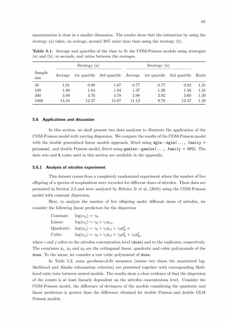
65
maximization is done in a smaller dimension. The results show that the estimation by using thestrategy (a) takes, on average, around 30% more time than using the strategy (b).
Table 5.1. Average and quartiles of the time to fit the COM-Poisson models using strategies(a) and (b), in seconds, and ratios between the averages.
Strategy (a) Strategy (b)Samplesize Average 1st quartile 3rd quartile Average 1st quartile 3rd quartile Ratio
50 1.01 0.98 1.07 0.77 0.77 0.82 1.31100 1.80 1.64 1.94 1.37 1.26 1.50 1.31300 3.89 3.76 4.78 2.98 2.92 3.60 1.301000 14.24 12.37 15.87 11.13 9.70 12.47 1.28
5.6 Applications and discussion
In this section, we shall present two data analyzes to illustrate the application of theCOM-Poisson model with varying dispersion. We compare the results of the COM-Poisson modelwith the double generalized linear models approach, fitted using dglm::dglm(..., family =poisson), and double Poisson model, fitted using gamlss::gamlss(..., family = DPO). Thedata sets and R codes used in this section are available in the appendix.
5.6.1 Analysis of nitrofen experiment
This dataset comes from a completely randomized experiment where the number of liveoffspring of a species of zooplankton were recorded for different doses of nitrofen. These data arepresented in Section 2.3 and were analyzed by Ribeiro Jr et al. (2018) using the COM-Poissonmodel with constant dispersion.
Here, to analyze the number of live offspring under different doses of nitrofen, weconsider the following linear predictors for the dispersion
Constant: log(νij) = γ0,Linear: log(νij) = γ0 + γ1x1i,Quadratic: log(νij) = γ0 + γ1x1i + γ2x2
2i eCubic: log(νij) = γ0 + γ1x1i + γ2x2
2i + γ3x33i,
where i and j refers to the nitrofen concentration level (dose) and to the replicates, respectively.The covariates x1, x2 and x3 are the orthogonal linear, quadratic and cubic polynomials of thedose. To the mean, we consider a raw cubic polynomial of dose.
In Table 5.2, some goodness-of-fit measures (minus two times the maximized log-likelihood and Akaike information criterion) are presented together with corresponding likeli-hood ratio tests between nested models. The results show a clear evidence of that the dispersionof the counts is at least linearly dependent on the nitrofen concentration level. Consider theCOM-Poisson model, the difference of deviances of the models considering the quadratic andlinear predictors is greater than the difference obtained for double Poisson and double GLMPoisson models.
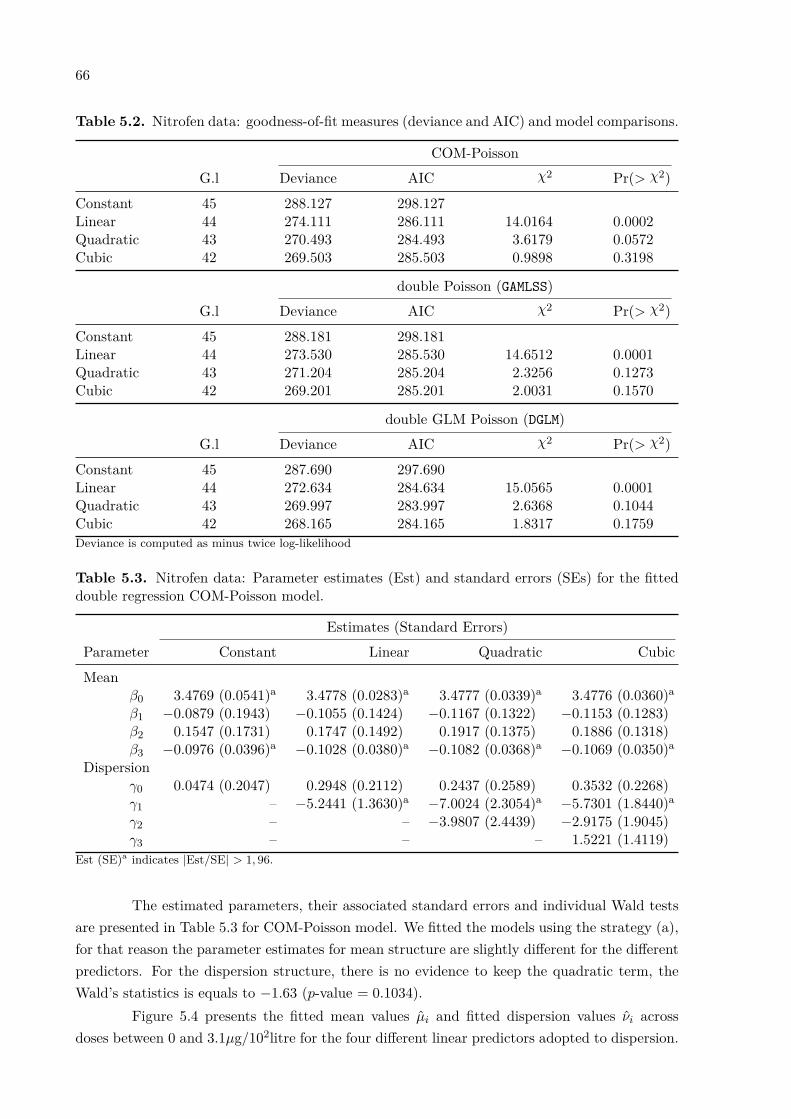
66
Table 5.2. Nitrofen data: goodness-of-fit measures (deviance and AIC) and model comparisons.
COM-PoissonG.l Deviance AIC χ2 Pr(> χ2)
Constant 45 288.127 298.127Linear 44 274.111 286.111 14.0164 0.0002Quadratic 43 270.493 284.493 3.6179 0.0572Cubic 42 269.503 285.503 0.9898 0.3198
double Poisson (GAMLSS)G.l Deviance AIC χ2 Pr(> χ2)
Constant 45 288.181 298.181Linear 44 273.530 285.530 14.6512 0.0001Quadratic 43 271.204 285.204 2.3256 0.1273Cubic 42 269.201 285.201 2.0031 0.1570
double GLM Poisson (DGLM)G.l Deviance AIC χ2 Pr(> χ2)
Constant 45 287.690 297.690Linear 44 272.634 284.634 15.0565 0.0001Quadratic 43 269.997 283.997 2.6368 0.1044Cubic 42 268.165 284.165 1.8317 0.1759Deviance is computed as minus twice log-likelihood
Table 5.3. Nitrofen data: Parameter estimates (Est) and standard errors (SEs) for the fitteddouble regression COM-Poisson model.
Estimates (Standard Errors)Parameter Constant Linear Quadratic CubicMean
β0 3.4769 (0.0541)a 3.4778 (0.0283)a 3.4777 (0.0339)a 3.4776 (0.0360)a
β1 −0.0879 (0.1943) −0.1055 (0.1424) −0.1167 (0.1322) −0.1153 (0.1283)β2 0.1547 (0.1731) 0.1747 (0.1492) 0.1917 (0.1375) 0.1886 (0.1318)β3 −0.0976 (0.0396)a −0.1028 (0.0380)a −0.1082 (0.0368)a −0.1069 (0.0350)a
Dispersionγ0 0.0474 (0.2047) 0.2948 (0.2112) 0.2437 (0.2589) 0.3532 (0.2268)γ1 – −5.2441 (1.3630)a −7.0024 (2.3054)a −5.7301 (1.8440)a
γ2 – – −3.9807 (2.4439) −2.9175 (1.9045)γ3 – – – 1.5221 (1.4119)
Est (SE)a indicates |Est/SE| > 1, 96.
The estimated parameters, their associated standard errors and individual Wald testsare presented in Table 5.3 for COM-Poisson model. We fitted the models using the strategy (a),for that reason the parameter estimates for mean structure are slightly different for the differentpredictors. For the dispersion structure, there is no evidence to keep the quadratic term, theWald’s statistics is equals to −1.63 (p-value = 0.1034).
Figure 5.4 presents the fitted mean values µ̂i and fitted dispersion values ν̂i acrossdoses between 0 and 3.1µg/102litre for the four different linear predictors adopted to dispersion.
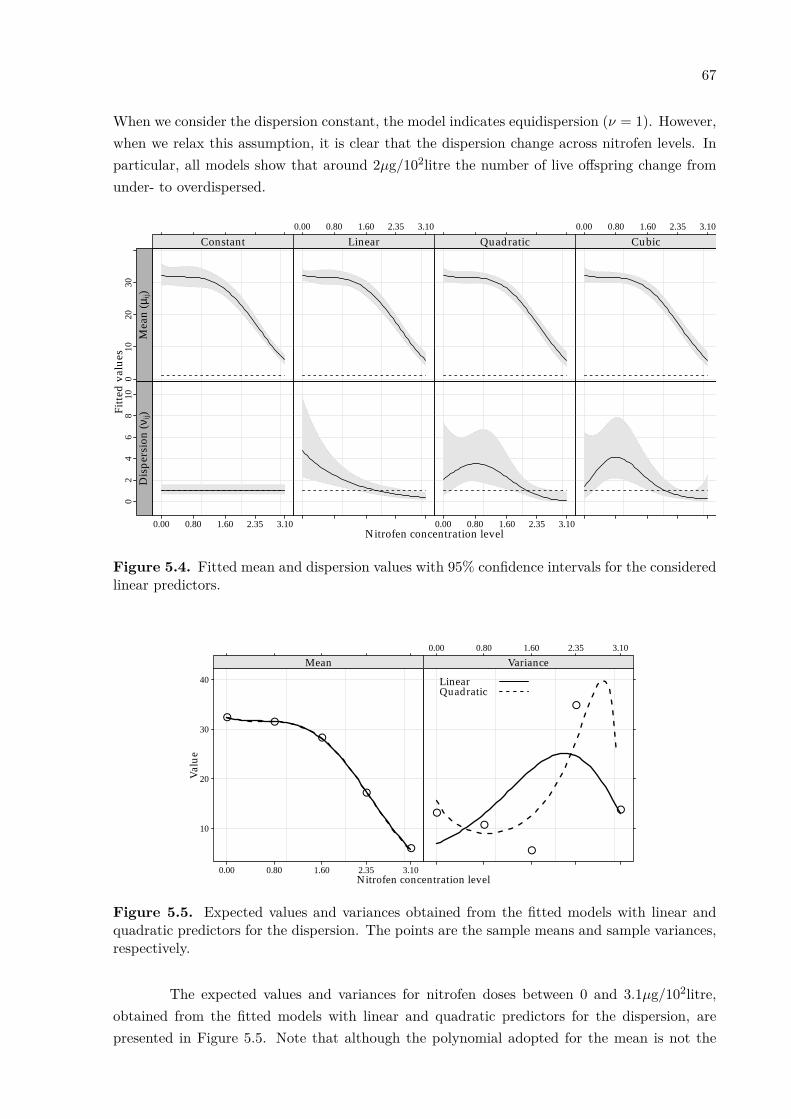
67
When we consider the dispersion constant, the model indicates equidispersion (ν = 1). However,when we relax this assumption, it is clear that the dispersion change across nitrofen levels. Inparticular, all models show that around 2µg/102litre the number of live offspring change fromunder- to overdispersed.
Nitrofen concentration level
Fitt
ed v
alue
s0
1020
30
Constant
Mea
n (µ
ij)
0.00 0.80 1.60 2.35 3.10
Linear Quadratic0.00 0.80 1.60 2.35 3.10
Cubic
02
46
810
0.00 0.80 1.60 2.35 3.10
Dis
pers
ion
(νij)
0.00 0.80 1.60 2.35 3.10
Figure 5.4. Fitted mean and dispersion values with 95% confidence intervals for the consideredlinear predictors.
Nitrofen concentration level
Val
ue
10
20
30
40
0.00 0.80 1.60 2.35 3.10
●●
●
●
●
Mean0.00 0.80 1.60 2.35 3.10
●
●
●
●
●
Variance
LinearQuadratic
Figure 5.5. Expected values and variances obtained from the fitted models with linear andquadratic predictors for the dispersion. The points are the sample means and sample variances,respectively.
The expected values and variances for nitrofen doses between 0 and 3.1µg/102litre,obtained from the fitted models with linear and quadratic predictors for the dispersion, arepresented in Figure 5.5. Note that although the polynomial adopted for the mean is not the
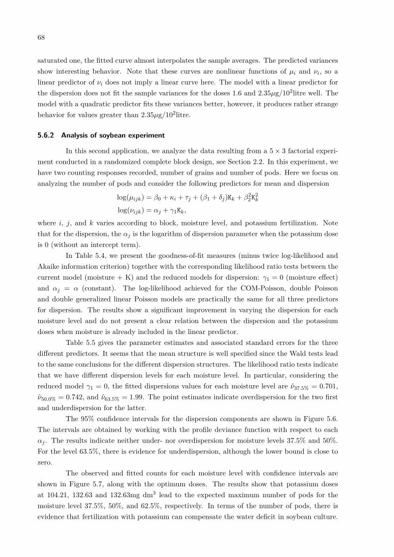
68
saturated one, the fitted curve almost interpolates the sample averages. The predicted variancesshow interesting behavior. Note that these curves are nonlinear functions of µi and νi, so alinear predictor of νi does not imply a linear curve here. The model with a linear predictor forthe dispersion does not fit the sample variances for the doses 1.6 and 2.35µg/102litre well. Themodel with a quadratic predictor fits these variances better, however, it produces rather strangebehavior for values greater than 2.35µg/102litre.
5.6.2 Analysis of soybean experiment
In this second application, we analyze the data resulting from a 5 × 3 factorial experi-ment conducted in a randomized complete block design, see Section 2.2. In this experiment, wehave two counting responses recorded, number of grains and number of pods. Here we focus onanalyzing the number of pods and consider the following predictors for mean and dispersion
log(µijk) = β0 + κi + τj + (β1 + δj)Kk + β22K2
k
log(νijk) = αj + γ1Kk,
where i, j, and k varies according to block, moisture level, and potassium fertilization. Notethat for the dispersion, the αj is the logarithm of dispersion parameter when the potassium doseis 0 (without an intercept term).
In Table 5.4, we present the goodness-of-fit measures (minus twice log-likelihood andAkaike information criterion) together with the corresponding likelihood ratio tests between thecurrent model (moisture + K) and the reduced models for dispersion: γ1 = 0 (moisture effect)and αj = α (constant). The log-likelihood achieved for the COM-Poisson, double Poissonand double generalized linear Poisson models are practically the same for all three predictorsfor dispersion. The results show a significant improvement in varying the dispersion for eachmoisture level and do not present a clear relation between the dispersion and the potassiumdoses when moisture is already included in the linear predictor.
Table 5.5 gives the parameter estimates and associated standard errors for the threedifferent predictors. It seems that the mean structure is well specified since the Wald tests leadto the same conclusions for the different dispersion structures. The likelihood ratio tests indicatethat we have different dispersion levels for each moisture level. In particular, considering thereduced model γ1 = 0, the fitted dispersions values for each moisture level are ν̂37.5% = 0.701,ν̂50.0% = 0.742, and ν̂63.5% = 1.99. The point estimates indicate overdispersion for the two firstand underdispersion for the latter.
The 95% confidence intervals for the dispersion components are shown in Figure 5.6.The intervals are obtained by working with the profile deviance function with respect to eachαj . The results indicate neither under- nor overdispersion for moisture levels 37.5% and 50%.For the level 63.5%, there is evidence for underdispersion, although the lower bound is close tozero.
The observed and fitted counts for each moisture level with confidence intervals areshown in Figure 5.7, along with the optimum doses. The results show that potassium dosesat 104.21, 132.63 and 132.63mg dm3 lead to the expected maximum number of pods for themoisture level 37.5%, 50%, and 62.5%, respectively. In terms of the number of pods, there isevidence that fertilization with potassium can compensate the water deficit in soybean culture.
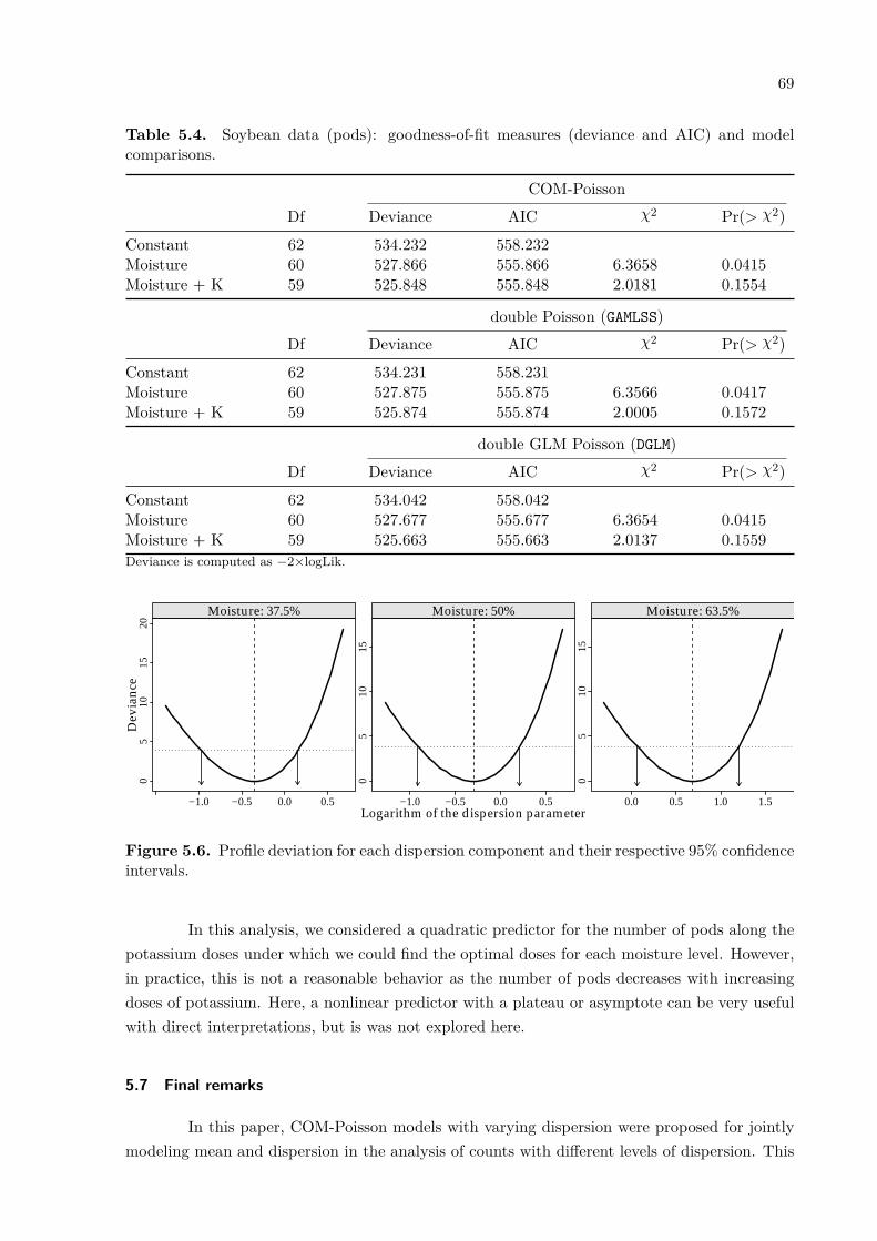
69
Table 5.4. Soybean data (pods): goodness-of-fit measures (deviance and AIC) and modelcomparisons.
COM-PoissonDf Deviance AIC χ2 Pr(> χ2)
Constant 62 534.232 558.232Moisture 60 527.866 555.866 6.3658 0.0415Moisture + K 59 525.848 555.848 2.0181 0.1554
double Poisson (GAMLSS)Df Deviance AIC χ2 Pr(> χ2)
Constant 62 534.231 558.231Moisture 60 527.875 555.875 6.3566 0.0417Moisture + K 59 525.874 555.874 2.0005 0.1572
double GLM Poisson (DGLM)Df Deviance AIC χ2 Pr(> χ2)
Constant 62 534.042 558.042Moisture 60 527.677 555.677 6.3654 0.0415Moisture + K 59 525.663 555.663 2.0137 0.1559Deviance is computed as −2×logLik.
Logarithm of the dispersion parameter
Dev
ianc
e0
510
1520
−1.0 −0.5 0.0 0.5
Moisture: 37.5%
05
1015
−1.0 −0.5 0.0 0.5
Moisture: 50%
05
1015
0.0 0.5 1.0 1.5
Moisture: 63.5%
Figure 5.6. Profile deviation for each dispersion component and their respective 95% confidenceintervals.
In this analysis, we considered a quadratic predictor for the number of pods along thepotassium doses under which we could find the optimal doses for each moisture level. However,in practice, this is not a reasonable behavior as the number of pods decreases with increasingdoses of potassium. Here, a nonlinear predictor with a plateau or asymptote can be very usefulwith direct interpretations, but is was not explored here.
5.7 Final remarks
In this paper, COM-Poisson models with varying dispersion were proposed for jointlymodeling mean and dispersion in the analysis of counts with different levels of dispersion. This
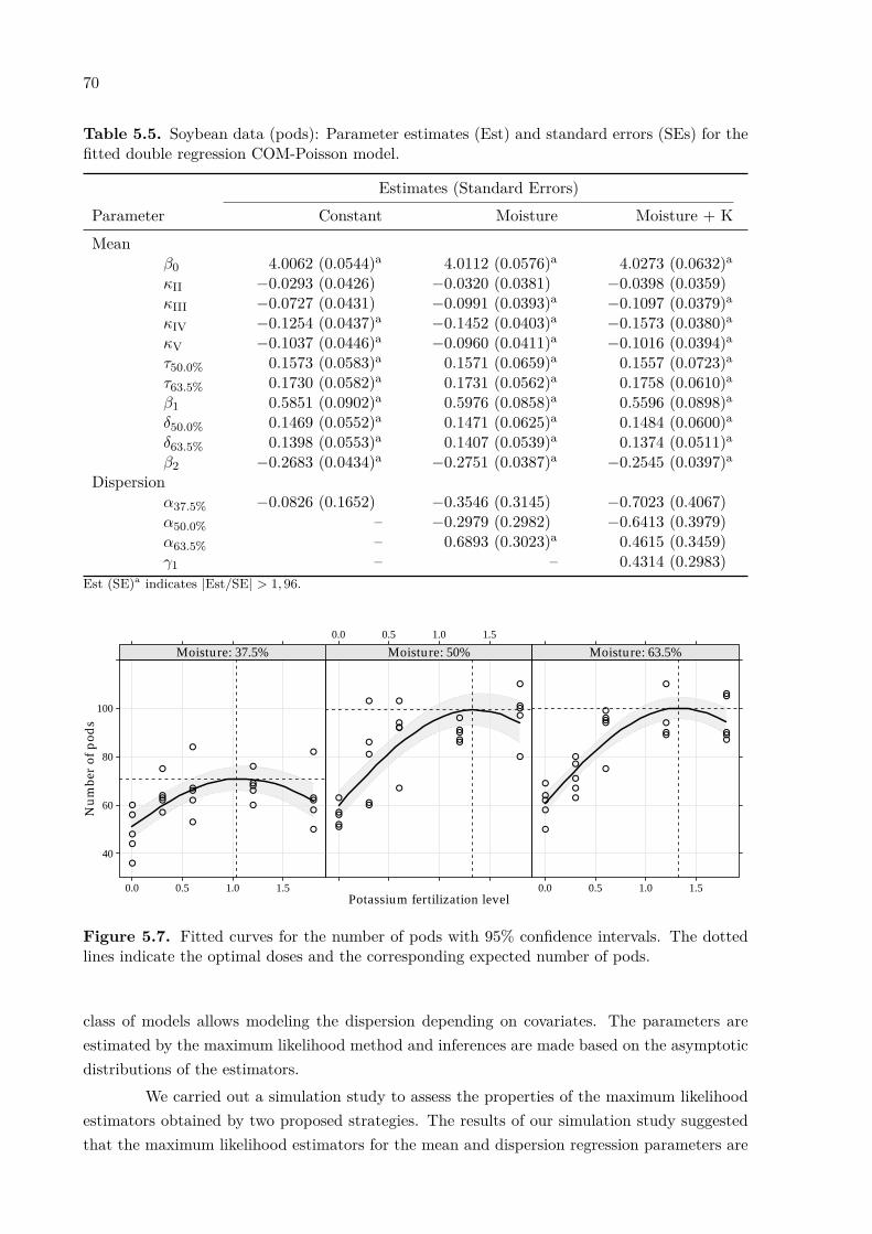
70
Table 5.5. Soybean data (pods): Parameter estimates (Est) and standard errors (SEs) for thefitted double regression COM-Poisson model.
Estimates (Standard Errors)Parameter Constant Moisture Moisture + KMean
β0 4.0062 (0.0544)a 4.0112 (0.0576)a 4.0273 (0.0632)a
κII −0.0293 (0.0426) −0.0320 (0.0381) −0.0398 (0.0359)κIII −0.0727 (0.0431) −0.0991 (0.0393)a −0.1097 (0.0379)a
κIV −0.1254 (0.0437)a −0.1452 (0.0403)a −0.1573 (0.0380)a
κV −0.1037 (0.0446)a −0.0960 (0.0411)a −0.1016 (0.0394)a
τ50.0% 0.1573 (0.0583)a 0.1571 (0.0659)a 0.1557 (0.0723)a
τ63.5% 0.1730 (0.0582)a 0.1731 (0.0562)a 0.1758 (0.0610)a
β1 0.5851 (0.0902)a 0.5976 (0.0858)a 0.5596 (0.0898)a
δ50.0% 0.1469 (0.0552)a 0.1471 (0.0625)a 0.1484 (0.0600)a
δ63.5% 0.1398 (0.0553)a 0.1407 (0.0539)a 0.1374 (0.0511)a
β2 −0.2683 (0.0434)a −0.2751 (0.0387)a −0.2545 (0.0397)a
Dispersionα37.5% −0.0826 (0.1652) −0.3546 (0.3145) −0.7023 (0.4067)α50.0% – −0.2979 (0.2982) −0.6413 (0.3979)α63.5% – 0.6893 (0.3023)a 0.4615 (0.3459)γ1 – – 0.4314 (0.2983)
Est (SE)a indicates |Est/SE| > 1, 96.
Potassium fertilization level
Num
ber
of p
ods
40
60
80
100
0.0 0.5 1.0 1.5
●
●
●●
●
●
●●
●●
●
●
●
●
●●
●
●
●
●
●
●
●
●
●
Moisture: 37.5%0.0 0.5 1.0 1.5
●
●
●
●
●
●
● ●
●
●
●
●
● ●
●
●
●
●
●
●
●
●
●
●
●
Moisture: 50%
0.0 0.5 1.0 1.5
●
●
●
●
●
●
●
●●
●
●
●
●
● ●
●
●
●
●●
●
●
●
●
Moisture: 63.5%
Figure 5.7. Fitted curves for the number of pods with 95% confidence intervals. The dottedlines indicate the optimal doses and the corresponding expected number of pods.
class of models allows modeling the dispersion depending on covariates. The parameters areestimated by the maximum likelihood method and inferences are made based on the asymptoticdistributions of the estimators.
We carried out a simulation study to assess the properties of the maximum likelihoodestimators obtained by two proposed strategies. The results of our simulation study suggestedthat the maximum likelihood estimators for the mean and dispersion regression parameters are

71
unbiased and consistent. The comparison of the strategies for maximum likelihood estimationindicate that using the strategy (a) (maximization of conditional likelihood) reduces the fittingtimes and leads to inferences quite similar to the strategy (b) (maximization of full likelihood).However, studies regarding the coverage rate of confidence intervals and the evaluation of type1 errors in hypothesis testing are necessary.
The methodology is applied to analyze two count datasets obtained from planned ex-periments. We compared the COM-Poisson models with double generalized linear models andGAMLSS approach. The proposal presented improvements in terms of fitting data when com-pared to the conventional COM-Poisson with constant dispersion and was competitive with thedouble generalized linear models and GALMSS based on double Poisson distribution.
For future work, simulation studies are necessary in order to evaluate the robustnessof the model. In addition, as an improvement in the case study analysis, considering nonlinearpredictors for the mean can be useful in order to avoid the use of high-order polynomials and toimpose biological restrictions.
References References
Aitkin, M. (1987). “Modelling Variance Heterogeneity in Normal Regression Using GLIM”. In:Journal of the Royal Statistical Society. Series C (Applied Statistics) 36.3, pp. 332–339.
Andersen, D. A. and W. H. Bonat (2017). “Double Generalized Linear Compound Poissonmodels to Insurance Claims Data”. In: Electronic Journal of Applied Statistical Analysis 10.2.
Efron, B. (1986). “Double Exponential Families and Their Use in Generalized Linear Regression”.In: Journal of the American Statistical Association 84.395, pp. 709–721.
Gilbert, P. and R. Varadhan (2016). numDeriv: Accurate Numerical Derivatives. R packageversion 2016.8-1.
McCullagh, P. and J. A. Nelder (1989). Generalized Linear Models. 2nd edition. Monographs onStatistics and Applied Probability. London: Chapman & Hall.
Nelder, J. A. and R. W. M. Wedderburn (1972). “Generalized Linear Models”. In: Journal ofthe Royal Statistical Society. Series A (General) 135, pp. 370–384.
Paula, G. A. (2013). “On diagnostics in double generalized linear models”. In: ComputationalStatistics & Data Analysis 68, pp. 44–51.
Pregibon, D. (1984). “Review: P. McCullagh, J. A. Nelder, Generalized Linear Models””. In:The Annals of Statistics 12.4, pp. 1589–1596.
R Core Team (2018). R: A Language and Environment for Statistical Computing. R Foundationfor Statistical Computing. Vienna, Austria.
Ribeiro Jr, E. E., W. M. Zeviani, W. H. Bonat, C. G. B. Demétrio, and J. Hinde (2018).“Reparametrization of COM-Poisson Regression Models with Applications in the Analysis ofExperimental Data”. In: arXiv (Statistics Applications and Statistics Methodology).
Rigby, R. A. and D. M. Stasinopoulos (2005). “Generalized additive models for location, scaleand shape (with discussion)”. In: Journal of the Royal Statistical Society. Series C (AppliedStatistics) 54.3, pp. 507–554.
72
Sellers, K. F. and G. Shmueli (2010). “A flexible regression model for count data”. In: Annals ofApplied Statistics 4.2, pp. 943–961.
Shmueli, G., T. P. Minka, J. B. Kadane, S. Borle, and P. Boatwright (2005). “A useful dis-tribution for fitting discrete data: Revival of the Conway-Maxwell-Poisson distribution”. In:Journal of the Royal Statistical Society. Series C (Applied Statistics) 54.1, pp. 127–142.
Smyth, G. K. (1988). “Generalized Linear Models with Varying Dispersion”. In: Journal of theRoyal Statistical Society. Series B (Methodological) 51.1, pp. 47–60.
Smyth, G. K. and A. P. Verbyla (1999). “Adjusted likelihood methods for modelling dispersionin generalized linear models”. In: Environmetrics 10.6, pp. 695–709.
Vieira, A. M., R. A. Leandro, C. G. Demétrio, and G. Molenberghs (2011). “Double generalizedlinear model for tissue culture proportion data: a Bayesian perspective”. In: Journal of AppliedStatistics 38.8, pp. 1717–1731.
Zou, Y., S. R. Geedipally, and D. Lord (2013). “Evaluating the double Poisson generalized linearmodel”. In: Accident Analysis and Prevention 59, pp. 497–505.
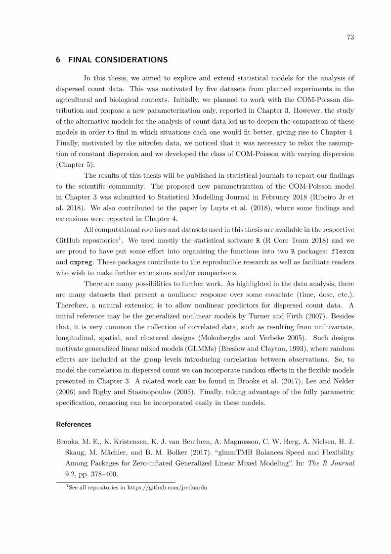
73
6 FINAL CONSIDERATIONS
In this thesis, we aimed to explore and extend statistical models for the analysis ofdispersed count data. This was motivated by five datasets from planned experiments in theagricultural and biological contexts. Initially, we planned to work with the COM-Poisson dis-tribution and propose a new parameterization only, reported in Chapter 3. However, the studyof the alternative models for the analysis of count data led us to deepen the comparison of thesemodels in order to find in which situations each one would fit better, giving rise to Chapter 4.Finally, motivated by the nitrofen data, we noticed that it was necessary to relax the assump-tion of constant dispersion and we developed the class of COM-Poisson with varying dispersion(Chapter 5).
The results of this thesis will be published in statistical journals to report our findingsto the scientific community. The proposed new parametrization of the COM-Poisson modelin Chapter 3 was submitted to Statistical Modelling Journal in February 2018 (Ribeiro Jr etal. 2018). We also contributed to the paper by Luyts et al. (2018), where some findings andextensions were reported in Chapter 4.
All computational routines and datasets used in this thesis are available in the respectiveGitHub repositories1. We used mostly the statistical software R (R Core Team 2018) and weare proud to have put some effort into organizing the functions into two R packages: flexcmand cmpreg. These packages contribute to the reproducible research as well as facilitate readerswho wish to make further extensions and/or comparisons.
There are many possibilities to further work. As highlighted in the data analysis, thereare many datasets that present a nonlinear response over some covariate (time, dose, etc.).Therefore, a natural extension is to allow nonlinear predictors for dispersed count data. Ainitial reference may be the generalized nonlinear models by Turner and Firth (2007). Besidesthat, it is very common the collection of correlated data, such as resulting from multivariate,longitudinal, spatial, and clustered designs (Molenberghs and Verbeke 2005). Such designsmotivate generalized linear mixed models (GLMMs) (Breslow and Clayton, 1993), where randomeffects are included at the group levels introducing correlation between observations. So, tomodel the correlation in dispersed count we can incorporate random effects in the flexible modelspresented in Chapter 3. A related work can be found in Brooks et al. (2017), Lee and Nelder(2006) and Rigby and Stasinopoulos (2005). Finally, taking advantage of the fully parametricspecification, censoring can be incorporated easily in these models.
References References
Brooks, M. E., K. Kristensen, K. J. van Benthem, A. Magnusson, C. W. Berg, A. Nielsen, H. J.Skaug, M. Mächler, and B. M. Bolker (2017). “glmmTMB Balances Speed and FlexibilityAmong Packages for Zero-inflated Generalized Linear Mixed Modeling”. In: The R Journal9.2, pp. 378–400.1See all repositories in https://github.com/jreduardo
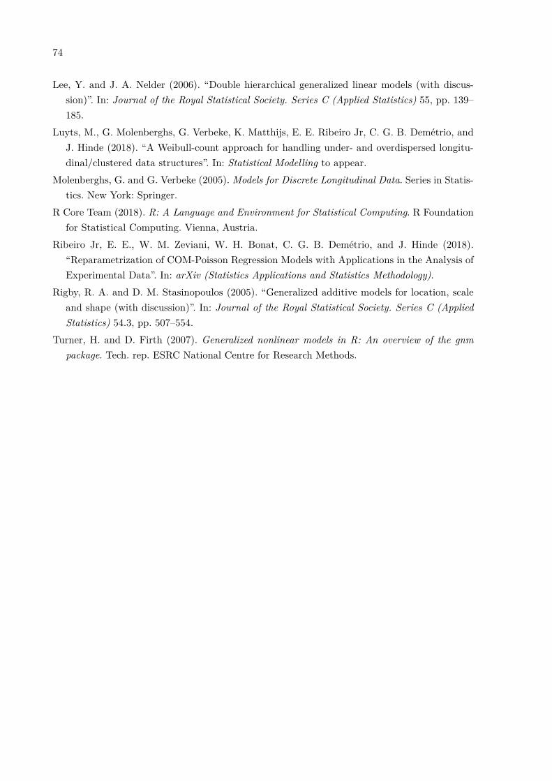
74
Lee, Y. and J. A. Nelder (2006). “Double hierarchical generalized linear models (with discus-sion)”. In: Journal of the Royal Statistical Society. Series C (Applied Statistics) 55, pp. 139–185.
Luyts, M., G. Molenberghs, G. Verbeke, K. Matthijs, E. E. Ribeiro Jr, C. G. B. Demétrio, andJ. Hinde (2018). “A Weibull-count approach for handling under- and overdispersed longitu-dinal/clustered data structures”. In: Statistical Modelling to appear.
Molenberghs, G. and G. Verbeke (2005). Models for Discrete Longitudinal Data. Series in Statis-tics. New York: Springer.
R Core Team (2018). R: A Language and Environment for Statistical Computing. R Foundationfor Statistical Computing. Vienna, Austria.
Ribeiro Jr, E. E., W. M. Zeviani, W. H. Bonat, C. G. B. Demétrio, and J. Hinde (2018).“Reparametrization of COM-Poisson Regression Models with Applications in the Analysis ofExperimental Data”. In: arXiv (Statistics Applications and Statistics Methodology).
Rigby, R. A. and D. M. Stasinopoulos (2005). “Generalized additive models for location, scaleand shape (with discussion)”. In: Journal of the Royal Statistical Society. Series C (AppliedStatistics) 54.3, pp. 507–554.
Turner, H. and D. Firth (2007). Generalized nonlinear models in R: An overview of the gnmpackage. Tech. rep. ESRC National Centre for Research Methods.
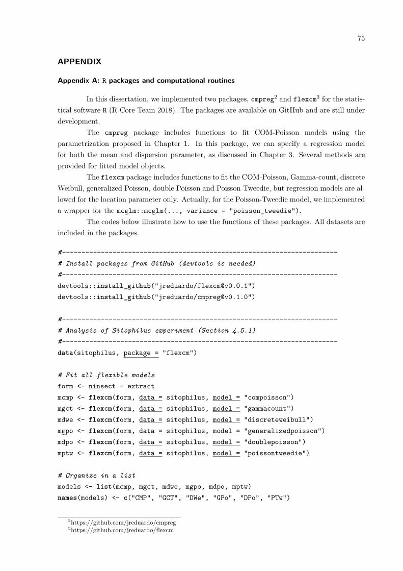
75
APPENDIX
Appendix A: R packages and computational routines
In this dissertation, we implemented two packages, cmpreg2 and flexcm3 for the statis-tical software R (R Core Team 2018). The packages are available on GitHub and are still underdevelopment.
The cmpreg package includes functions to fit COM-Poisson models using theparametrization proposed in Chapter 1. In this package, we can specify a regression modelfor both the mean and dispersion parameter, as discussed in Chapter 3. Several methods areprovided for fitted model objects.
The flexcm package includes functions to fit the COM-Poisson, Gamma-count, discreteWeibull, generalized Poisson, double Poisson and Poisson-Tweedie, but regression models are al-lowed for the location parameter only. Actually, for the Poisson-Tweedie model, we implementeda wrapper for the mcglm::mcglm(..., variance = "poisson_tweedie").
The codes below illustrate how to use the functions of these packages. All datasets areincluded in the packages.
#-----------------------------------------------------------------------# Install packages from GitHub (devtools is needed)#-----------------------------------------------------------------------devtools::install_github("jreduardo/[email protected]")devtools::install_github("jreduardo/[email protected]")
#-----------------------------------------------------------------------# Analysis of Sitophilus experiment (Section 4.5.1)#-----------------------------------------------------------------------data(sitophilus, package = "flexcm")
# Fit all flexible modelsform <- ninsect ~ extractmcmp <- flexcm(form, data = sitophilus, model = "compoisson")mgct <- flexcm(form, data = sitophilus, model = "gammacount")mdwe <- flexcm(form, data = sitophilus, model = "discreteweibull")mgpo <- flexcm(form, data = sitophilus, model = "generalizedpoisson")mdpo <- flexcm(form, data = sitophilus, model = "doublepoisson")mptw <- flexcm(form, data = sitophilus, model = "poissontweedie")
# Organize in a listmodels <- list(mcmp, mgct, mdwe, mgpo, mdpo, mptw)names(models) <- c("CMP", "GCT", "DWe", "GPo", "DPo", "PTw")
2https://github.com/jreduardo/cmpreg3https://github.com/jreduardo/flexcm
76
# Methods for objects for the class 'flexcm'lapply(models, print)lapply(models, summary)lapply(models, equitest)lapply(models, logLik)lapply(models, AIC)lapply(models, fitted)
# Prediction intervalsnewdata <- unique(sitophilus[, "extract", drop = FALSE])lapply(models, function(model) {
predict(model,newdata = newdata,type = "response",interval = "confidence",level = 0.95,augment_data = TRUE)
})
#-----------------------------------------------------------------------# Analysis of nitrofen experiment (Sections 3.6.3 and 5.6.1)#-----------------------------------------------------------------------data(nitrofen, package = "cmpreg")
# Linear predictorspo <- function(x, degree) c(poly(x, degree, raw = FALSE)[, degree])form0 <- ~ 1form1 <- ~ po(dose, 1)form2 <- ~ po(dose, 1) + po(dose, 2)form3 <- ~ po(dose, 1) + po(dose, 2) + po(dose, 3)
# Organize in a listformulas <- list(form0, form1, form2, form3)names(formulas) <- c("Constant", "Linear", "Quadratic", "Cubic")
# Fit CMP models using joint strategymodelscmp <-
lapply(formulas, function(form) {cmp(novos ~ dose + I(dose^2) + I(dose^3),
dformula = form,data = nitrofen)
})
77
# Fit double Poisson models (gamlss and gamlss.dist are needed)modelsdpo <-
map(formulas, function(form) {gamlss::gamlss(novos ~ dose + I(dose^2) + I(dose^3),
sigma.formula = form,family = gamlss.dist::DPO,data = nitrofen,trace = FALSE)
})
# Fit double Generalized Linear Poisson model (dglm is needed)modelsglm <-
map(formulas, function(form) {dglm::dglm(novos ~ dose + I(dose^2) + I(dose^3),
dformula = form,family = poisson,data = nitrofen)
})
# Methods for objects of class 'cmpreg'lapply(modelscmp, summary)lapply(modelscmp, logLik)lrtest(modelscmp) # or anova(modelscmp)
# Some type of residualsmodel <- modelscmp[[2]]plot(fitted(model), residuals(model))plot(fitted(model), residuals(model, type = "pearson"))
# Prediction with confidence intervalsnewdf <- nitrofen[c(1, 11, 21, 31), -2, drop = FALSE]predict(object = model,
newdata = newdf,what = "all",type = "response")

78
79
BIBLIOGRAPHY
Aitkin, M. (1987). “Modelling Variance Heterogeneity in Normal Regression Using GLIM”. In:Journal of the Royal Statistical Society. Series C (Applied Statistics) 36.3, pp. 332–339.
Andersen, D. A. and W. H. Bonat (2017). “Double Generalized Linear Compound Poissonmodels to Insurance Claims Data”. In: Electronic Journal of Applied Statistical Analysis 10.2.
Bailer, A. and J. Oris (1994). “Assessing toxicity of pollutants in aquatic systems”. In: In CaseStudies in Biometry, pp. 25–40.
Bonat, W. H. (2018). “Multiple Response Variables Regression Models in R: The mcglm Pack-age”. In: Journal of Statistical Software 84.4, pp. 1–30.
Bonat, W. H. and B. Jørgensen (2016). “Multivariate covariance generalized linear models”. In:Journal of the Royal Statistical Society. Series C (Applied Statistics).
Bonat, W. H., B. Jørgensen, C. C. Kokonendji, and J. Hinde (2018). “Extended Poisson-Tweedie:properties and regression model for count data”. In: Statistical Modelling 18.1, pp. 24–49.
Bonat, W. H., W. M. Zeviani, and E. E. Ribeiro Jr (2017). Regression Models for Count Data:beyond Poisson model. Goiás, Brazil: XV EMR - Brazilian Regression Model School.
Brooks, M. E., K. Kristensen, K. J. van Benthem, A. Magnusson, C. W. Berg, A. Nielsen, H. J.Skaug, M. Mächler, and B. M. Bolker (2017). “glmmTMB Balances Speed and FlexibilityAmong Packages for Zero-inflated Generalized Linear Mixed Modeling”. In: The R Journal9.2, pp. 378–400.
Cameron, A. C. and P. K. Trivedi (2013). Regression Analysis of Count Data. 2nd edition.Econometric Society Monographs. New York: Cambridge University press.
Chatla, S. B. and G. Shmueli (2018). “Efficient estimation of COM-Poisson regression and ageneralized additive model”. In: Computational Statistics & Data Analysis 121, pp. 71–89.
Consul, P. C. and F. Famoye (1992). “Generalized Poisson Regression Model”. In: Communica-tion in Statistics – Theory and Methods 21.1, pp. 89–109.
Consul, P. C. and G. C. Jain (1973). “A Generalization of the Poisson Distribution”. In: Tech-nometrics 15.4, pp. 791–799.
Cox, D. R. (1962). Renewal Theory. Monographs on Statistics and Applied Probability. London:Chapman & Hall.
Cox, D. R. and N. Reid (1987). “Orthogonality and Approximate Conditional Inference (withdiscussion)”. In: Journal of the Royal Statistical Society. Series B (Methodological) 49.1, pp. 1–39.
Daly, F. and R. Gaunt (2016). “The Conway-Maxwell-Poisson distribution: Distributional theoryand approximation”. In: ALEA, Latin American Journal of Probability and MathematicalStatistics 13, pp. 635–658.
Del Castillo, J. and M. Pérez-Casany (1998). “Weighted Poisson Distributions for Overdispersionand Underdispersion Situations”. In: Annals of the Institute of Statistical Mathematics 50.3,pp. 567–585.
80
Demétrio, C. G. B., J. Hinde, and R. A. Moral (2014). “Models for overdispersed data in ento-mology”. In: Ecological modelling applied to entomology. Springer, pp. 219–259.
Efron, B. (1986). “Double Exponential Families and Their Use in Generalized Linear Regression”.In: Journal of the American Statistical Association 84.395, pp. 709–721.
Gaunt, R., S. Iyengar, A. Olde Daalhuis, and B. Simsek (2017). “An asymptotic expansionfor the normalizing constant of the Conway-Maxwell-Poisson distribution”. In: Annals of theInstitute of Statistical Mathematics to appear.
Gilbert, P. and R. Varadhan (2016). numDeriv: Accurate Numerical Derivatives. R packageversion 2016.8-1.
Hilbe, J. M. (2014). Modeling Count Data. New York: Cambridge University press.Hinde, J. and C. G. B. Demétrio (1998). “Overdispersion: models and estimation”. In: Compu-
tational Statistics & Data Analysis 27.2, pp. 151–170.Huang, A. (2017). “Mean-parametrized Conway–Maxwell–Poisson regression models for dis-
persed counts”. In: Statistical Modelling 17.6, pp. 1–22.Johnson, N. L., A. W. Kemp, and S. Kotz (2005). Univariate Discrete Distributions. 3rd edition.
Series in Probability and Statistics. New Jersey: John Wiley & Sons.Jørgensen, B. (1997). The Theory of Dispersion Models. Monographs on Statistics and Applied
Probability. London: Chapman & Hall.Kanashiro, S., K. Minami, T. Jocys, C. T. dos Santos Dias, and A. R. Tavares (2008). “Alter-
native substrates to fern tree fiber in the production of ornamental bromeliad”. In: PesquisaAgropecuária Brasileira 43.10.
Klakattawi, H. S., V. Vinciotti, and K. Yu (2018). “A Simple and Adaptive Dispersion RegressionModel for Count Data”. In: Entropy 20.142.
Kokonendji, C. C. (2014). “Over- and Underdispersion Models”. In: ed. by N. Balakrishnan.John Wiley & Sons. Chap. 30, pp. 506–526.
Lee, Y. and J. A. Nelder (2006). “Double hierarchical generalized linear models (with discus-sion)”. In: Journal of the Royal Statistical Society. Series C (Applied Statistics) 55, pp. 139–185.
Lindsey, J. K. (1996). Parametric Statistical Inference. New York: Oxford University Press.Lord, D., S. R. Geedipally, and S. D. Guikema (2010). “Extension of the application of Conway-
Maxwell-Poisson models: Analyzing traffic crash data exhibiting underdispersion”. In: RiskAnalysis 30.8, pp. 1268–1276.
Lord, D., S. D. Guikema, and S. R. Geedipally (2008). “Application of the Conway-Maxwell-Poisson generalized linear model for analyzing motor vehicle crashes”. In: Accident Analysisand Prevention 40, pp. 1123–1134.
Luyts, M., G. Molenberghs, G. Verbeke, K. Matthijs, E. E. Ribeiro Jr, C. G. B. Demétrio, andJ. Hinde (2018). “A Weibull-count approach for handling under- and overdispersed longitu-dinal/clustered data structures”. In: Statistical Modelling to appear.
McCullagh, P. and J. A. Nelder (1989). Generalized Linear Models. 2nd edition. Monographs onStatistics and Applied Probability. London: Chapman & Hall.
81
Molenberghs, G. and G. Verbeke (2005). Models for Discrete Longitudinal Data. Series in Statis-tics. New York: Springer.
Molenberghs, G., G. Verbeke, and C. G. B. Demétrio (2007). “An extended random-effectsapproach to modelling repetead, overdispersed count data”. In: Lifetime Data Analysis 13,pp. 513–531.
Nakagawa, T. and S. Osaki (1975). “The Discrete Weibull Distribution”. In: IEEE Transactionson Reliability 24.5, pp. 300–301.
Nelder, J. A. and D. Pregibon (1987). “An Extended Quasi-likelihood Function”. In: Biometrika74.2, pp. 221–232.
Nelder, J. A. and R. W. M. Wedderburn (1972). “Generalized Linear Models”. In: Journal ofthe Royal Statistical Society. Series A (General) 135, pp. 370–384.
Nocedal, J. and S. J. Wright (2006). Numerical optimization. 2nd edition. Series in OperationsResearch. New York: Springer, p. 636. isbn: 0387987932.
Paula, G. A. (2013). “On diagnostics in double generalized linear models”. In: ComputationalStatistics & Data Analysis 68, pp. 44–51.
Pawitan, Y. (2001). In all likelihood: statistical modelling and inference using likelihood. NewYork: Oxford University Press.
Pregibon, D. (1984). “Review: P. McCullagh, J. A. Nelder, Generalized Linear Models””. In:The Annals of Statistics 12.4, pp. 1589–1596.
Puig, P. and J. Valero (2006). “Count data distributions: some characterizations with applica-tions”. In: Journal of the American Statistical Association 101.473, pp. 332–340.
R Core Team (2017). R: A Language and Environment for Statistical Computing. R Foundationfor Statistical Computing. Vienna, Austria.
R Core Team (2018). R: A Language and Environment for Statistical Computing. R Foundationfor Statistical Computing. Vienna, Austria.
Ribeiro Jr, E. E., W. M. Zeviani, W. H. Bonat, C. G. B. Demétrio, and J. Hinde (2018).“Reparametrization of COM-Poisson Regression Models with Applications in the Analysis ofExperimental Data”. In: arXiv (Statistics Applications and Statistics Methodology).
Ribeiro, L. P., J. D. Vendramim, K. U. Bicalho, M. S. Andrade, J. B. Fernandes, R. A. Moral,and C. G. B. Demétrio (2013). “Annona mucosa Jacq. (Annonaceae): A promising sourceof bioactive compounds against Sitophilus zeamais Mots. (Coleoptera: Curculionidae)”. In:Journal of Stored Products Research 55, pp. 6–14.
Rigby, R. A. and D. M. Stasinopoulos (2005). “Generalized additive models for location, scaleand shape (with discussion)”. In: Journal of the Royal Statistical Society. Series C (AppliedStatistics) 54.3, pp. 507–554.
Ross, G. J. S. (1970). “The Efficient Use of Function Minimization in Non-Linear Maximum-Likelihood Estimation”. In: Journal of the Royal Statistical Society. Series C (Applied Statis-tics) 19.3, pp. 205–221.
Salvador, E. (2008). “Evaluation of Alternative Substrates to the Xaxim dust for ’Ma-trogrossense’ fern (Poly Aureum) Cultivation”. In: Acta Horticulturae 779, pp. 547–554.
82
Sellers, K. F. and D. S. Morris (2017). “Underdispersion models: Models that are “under theradar””. In: Communication in Statistics – Theory and Methods 46.24, pp. 12075–12086.
Sellers, K. F. and G. Shmueli (2010). “A flexible regression model for count data”. In: Annals ofApplied Statistics 4.2, pp. 943–961.
Serafim, M. E., F. B. Ono, W. M. Zeviani, J. O. Novelino, and J. V. Silva (2012). “Umidade dosolo e doses de potássio na cultura da soja”. In: Revista Ciência Agronômica 43.2, pp. 222–227.
Shmueli, G., T. P. Minka, J. B. Kadane, S. Borle, and P. Boatwright (2005). “A useful dis-tribution for fitting discrete data: Revival of the Conway-Maxwell-Poisson distribution”. In:Journal of the Royal Statistical Society. Series C (Applied Statistics) 54.1, pp. 127–142.
Silva, A. M., P. E. Degrande, R. Suekane, M. G. Fernandes, and W. M. Zeviani (2012). “Impactode diferentes nı́veis de desfolha artificial nos estágios fenológicos do algodoeiro”. In: Revistade Ciências Agrárias 35.1, pp. 163–172.
Smyth, G. K. (1988). “Generalized Linear Models with Varying Dispersion”. In: Journal of theRoyal Statistical Society. Series B (Methodological) 51.1, pp. 47–60.
Smyth, G. K. and A. P. Verbyla (1999). “Adjusted likelihood methods for modelling dispersionin generalized linear models”. In: Environmetrics 10.6, pp. 695–709.
Steutel, F. W. and J. G. F. Thiemann (1989). “The gamma process and the Poisson distribution”.In: (Memorandum COSOR; Vol. 8924). Eindhoven: Technische Universiteit Eindhoven.
Turner, H. and D. Firth (2007). Generalized nonlinear models in R: An overview of the gnmpackage. Tech. rep. ESRC National Centre for Research Methods.
Vieira, A. M., R. A. Leandro, C. G. Demétrio, and G. Molenberghs (2011). “Double generalizedlinear model for tissue culture proportion data: a Bayesian perspective”. In: Journal of AppliedStatistics 38.8, pp. 1717–1731.
Wedderburn, R. W. M. (1974). “Quasi-Likelihood Functions, Generalized Linear Models, andthe Gauss-Newton Method”. In: Biometrika 61.3, p. 439.
Winkelmann, R. (1995). “Duration Dependence and Dispersion in Count-Data Models”. In:Journal of Business & Economic Statistics 13.4, pp. 467–474.
Winkelmann, R. (2008). Econometric Analysis of Count Data. 5th edition. Berlin, Heidelberg:Springer-Velag, p. 342.
Winkelmann, R. and K. F. Zimmermann (1994). “Count Data Models for Demographic Data”.In: Mathematical Population Studies 4.3, pp. 205–221.
Zamani, H. and N. Ismail (2012). “Functional Form for the Generalized Poisson RegressionModel”. In: Communication in Statistics – Theory and Methods 41, pp. 3666–3675.
Zeviani, W. M., P. J. Ribeiro Jr, W. H. Bonat, S. E. Shimakura, and J. A. Muniz (2014). “TheGamma-count distribution in the analysis of experimental underdispersed data”. In: Journalof Applied Statistics 41.12, pp. 2616–2626.
Zou, Y., S. R. Geedipally, and D. Lord (2013). “Evaluating the double Poisson generalized linearmodel”. In: Accident Analysis and Prevention 59, pp. 497–505.


![The Matrix Generalized Inverse Gaussian …baner029/papers/16/CMCPMF.pdfMatrix Generalized Inverse Gaussian (MGIG) distributions [3,10] are a family of distributions over the space](https://img.pdfslide.net/doc/110x75/5f04904f7e708231d40e9764/the-matrix-generalized-inverse-gaussian-baner029papers16-matrix-generalized-inverse.jpg)


![Package ‘tweedie’ - RPackage ‘tweedie’ December 14, 2017 Version 2.3.2 Date 2017-12-14 Title Evaluation of Tweedie Exponential Family Models Author Peter K. Dunn [cre, aut]](https://img.pdfslide.net/doc/110x75/5fe12382457901682c259167/package-atweediea-r-package-atweediea-december-14-2017-version-232.jpg)