UNIVERSITY OF WISCONSIN DEPARTMENT OF ... OF WISCONSIN DEPARTMENT OF BIOSTATISTICS AND MEDICAL INFORMATICS UNIVERSITY OF WISCONSIN DEPARTMENT OF BIOSTATISTICS AND MEDICAL INFORMATICS

UNIVERSITY OF WISCONSIN

DEPARTMENT OF BIOSTATISTICS AND MEDICAL INFORMATICS

UNIVERSITY OF WISCONSIN DEPARTMENT OF BIOSTATISTICS

AND MEDICAL INFORMATICS K6/446 Clinical Science Center

600 Highland Avenue Madison, Wisconsin 53792-4675

(608) 263-1706

Technical Report April 2010 # 210

A novel semiparametric regression method

for interval-censored data

Seungbong Han Adin-Cristian Andrei

Kam-Wah Tsui

A novel semiparametric regression method for interval-censored data

Seungbong Han 1, Adin-Cristian Andrei 2,∗, and Kam-Wah Tsui 1

1Department of Statistics, University of Wisconsin-Madison, MSC,

1300 University Avenue, Madison, WI, 53706, U.S.A.

2Department of Biostatistics and Medical Informatics, University of Wisconsin-Madison,

K6/428 CSC 600 Highland Avenue, Madison, WI, 53792-4675, U.S.A.

*email: [email protected]

Summary: In many medical studies, event times are recorded in an interval-censored (IC) format.

For example, in numerous cancer trials, time to disease relapse is only known to have occurred

between two consecutive clinic visits. Many existing modeling methods in the IC context are com-

putationally intensive and usually require numerous assumptions that could be unrealistic or difficult

to verify in practice. We propose a novel, flexible and computationally efficient modeling strategy

based on jackknife pseudo-observations (POs). The POs obtained based on nonparametric estimators

of the survival function are employed as outcomes in an equivalent, yet simpler regression model

that produces consistent covariate effect estimates. Hence, instead of operating in the IC context,

the problem is translated into the realm of generalized linear models, where numerous options are

available. Outcome transformations via appropriate link functions lead to familiar modeling contexts

such as the proportional hazards and proportional odds. Moreover, the methods developed are not

limited to these settings and have broader applicability. Simulations studies show that the proposed

methods produce virtually unbiased covariate effect estimates, even for moderate sample sizes. An

example from the International Breast Cancer Study Group (IBCSG) Trial VI further illustrates

the practical advantages of this new approach.

Key words: Interval-censoring; Pseudo-observations; Regression; Semiparametric; Survival anal-

ysis.

1

A novel semiparametric regression method for interval-censored data 1

1. Introduction

Interval-censored (IC) data are naturally and frequently encountered in numerous medical

studies involving event times. Instead of being observed exactly, the event of interest is known

to have occurred within a certain time interval, such as that between two consecutive patient

examinations. For example, in the IBCSG Trial VI (International Breast Cancer Study Group,

1996), time to cancer progression is known to have occurred between the latest cancer

progression-free visit and the date when disease-progression has been detected.

There is a rich literature in the area of modeling IC data, but a pervasive lack of soft-

ware availability prevents their routine use in practice. The proportional hazards setting

appears to be a favorite structural framework for methodology development (see, for example,

Finkelstein, 1986, Alioum and Commenges, 1996 or Satten, 1996). More recently, Betensky

et al. (2002) develop local likelihood estimation methods involving smoothing of the baseline

hazard function, while Cai and Betensky (2003) assume a piecewise-linear baseline hazard

and use penalized likelihood estimation methods. A useful alternative to the proportional

hazards model is the proportional odds model. In this context, Murphy et al. (1997) carry

out parameter and variance estimation via profile likelihood methods. Shen (1998) develops

consistent estimators for the baseline hazard and the regression parameters using sieve

maximum likelihood and monotone splines. In addition, Rabinowitz et al. (2000) propose an

approximate conditional likelihood-based model and Sun et al. (2007) develop goodness-of-

fit tests. Accelerated failure time models provide yet another useful methodological context,

such as in Betensky et al. (2001) and Li and Pu (2003). An asymptotically efficient sieve

maximum likelihood estimator is developed by Xue et al. (2006). For more on these and other

existing methods, one might consult Tian and Cai (2006) or Sun (2006). In practice, middle-

point imputation is used to substitute interval-censoring with right-censoring. Despite its

2

appeal, this oftentimes produces biased results, as discussed by Lindsey and Ryan (1998)

and illustrated in our simulations.

We propose a novel and easy to implement semiparametric IC data modeling strategy

in which the jackknife pseudo-observations (POs) (Quenouille, 1949 and Tukey, 1958) play

a fundamental role. Employed in linear regression analyses (Wu, 1986, Simonoff and Tsai,

1986), the POs use in event time settings is relatively recent and remains specific to right-

censored data contexts (see Andersen et al. (2003), Andersen et al. (2004) or Klein and

Andersen (2005)). For completeness, we briefly describe how POs are obtained. In general,

given an estimator θ of θ based on an i.i.d. sample T1, · · · , Tn and its version θ(−i) obtained

using the reduced sample T1, · · · , Ti−1, Ti+1, · · · , Tn, the ith pseudo-observation is defined as

νi = nθ−(n−1)θ(−i), where i = 1, · · · , n. For example, if θ = E(T ) and θ = n−1∑n

i=1 Ti is the

sample mean, then νi = Ti. However, when Ti is subject to interval-censoring, θ estimators

have no closed-form and νi 6= Ti.

Let Zi and S(t|Zi) = P (Ti > t|Zi) be the covariate vector and the conditional survival

function for individual i, respectively. Assume that one intends to construct a regression

model S(t|Zi) = A(t) − βT Zi, where t is fixed and A(t) is a function of time. Let S(t) be a

consistent estimator of the marginal survival function S(t) = P (Ti > t) of Ti, obtained in

nonparametric fashion or otherwise, and let S(−i)(t) be its reduced sample version with the ith

observation excluded. Using pseudo-observations, a simple, yet very direct modeling strategy

could be devised. We sketch a brief heuristic argument and recommend Andersen et al.

(2004) for further justification. Noting that S(t) = EZ{E[I(T > t)|Z]} = EZ [P (T > t|Z)],

it is natural to estimate S(t) by S(t) = n−1∑n

j=1 S(t|Zj) in which S(t|Zj) is a consistent

estimator for S(t|Zj) based on N samples. The leave-one-out estimator of S(t) is S(−i)(t) =

(n − 1)−1∑n

j=1,j 6=i S(t|Zj) where S(t|Zj) is a consistent estimator for S(t|Zj) based on n−1

reduced samples. When n is large, S(t|Z) and S(t|Z) will be approximately equal. Therefore,


the ith PO νi = nS(t)− (n−1)S(−i)(t) approximates S(t|Zi). Hence, ith PO νi might be used

as a substitute for S(t|Zi) in the desired regression model S(t|Zi) = A(t)−βT Zi. As detailed

at length in the next section, nonparametric estimation of S(t) will provide the POs used

in modeling. The implementation effort is minimal, therefore this method has an increased

potential for immediate use in biomedical data analyses. Considering the lack of public

software availability for more recent interval-censored data methodologies, this approach has

a obvious advantage.

The rest of this article is organized as follows: we present the IC data modeling strategy

in Section 2, while extensive simulation results showing excellent method performance in

moderate sample sizes are shown in Section 3. An application to the IBCSG Trial VI data

example constitutes Section 4, while further remarks are part of Section 5.

2. Pseudo-observation-based regression for IC data

Recently, POs have been used successfully in right-censored data modeling; examples include

Graw et al. (2009), Andersen et al. (2004), Andrei and Murray (2007), Liu et al. (2008) or

Logan et al. (2008). However, the use of POs in the interval-censored (IC) data context is

novel and constitutes the central theme of this research. Assume that the observed data

are an i.i.d. sample {(Li, Ri], Zi; i = 1, · · · , n}, where (Li, Ri] is the observation window

(censoring interval) for event time Ti and Zi is a p-dimensional vector of covariates for

subject i. Suppose that Ti is independent of (Li, Ri]. By convention, Li = Ri yields the exact

failure time Ti; Li = 0 produces left-censoring, while Ri = ∞ creates right-censoring. Let

S(t|Zi) = P (Ti > t|Zi) be the conditional survival function of Ti, given Zi, computed at a

fixed time t > 0. Our primary goal is to model a large class of outcomes g[S(t|Zi)], where

g(·) is a smooth link function. Assume that, for all t > 0 following model holds:

g[S(t|Zi)] = A(t) − βT Zi

4

where β is a p-dimensional covariate-effect vector and the intercept A(t) is a function of time.

For example, g(t)=log[−log(t)] leads to the proportional hazards model, while g(t)=log( t1−t

)

yields the proportional odds model. Needed to define the pseudo-observations (POs), let S(t)

be a consistent nonparametric estimator of the marginal survival function S(t) and S−i(t)

be its leave-ith-out version. Then, we define the ith PO as

νi(t) = ng{S(t)} − (n − 1)g{S−i(t)}.

It follows that g{S(t)} is a consistent estimator of g{S(t)} and, instead of regressing g{S(t|Zi)}

on Zi, we will regress νi(t) on Zi, thus regarding the POs as a valid substitute for g{S(t|Zi)}.

As pointed out by Tukey (1958), Andersen et al. (2004) or Graw et al. (2009), the POs could

be regarded as independent, for all practical purposes. Importantly, the function g(·) is part

of the PO definition. Authors such as Andersen et al. (2003) define the ith PO as ηi(t) =

nS(t)−(n−1)S−i(t) and fit the generalized linear model ηi(t) = g−1[A(t)−βZi], to estimate

β. We have not altered the definition of the PO, but simply applied the transformation to

the outcome g{S(t|Zi)} directly.

One may consider J > 2 distinct time points 0 < t1 < . . . < tJ < ∞ and construct

vector νi = {νi(t1), . . . , νi(tJ)}T of POs, for each individual i = 1, . . . , n. Recall that Zi =

(Zi1, . . . , Zip)T is a p-dimensional covariate vector and let α = {A(t1), . . . , A(tJ)}T , γ =

(αT , βT )T and B be a J × p-dimensional matrix whose rows are all equal to βT . Then, one

could obtain an estimate γ for γ by solving the following generalized estimating equations:

U(γ) =

n∑

i=1

Ui(γ) =

n∑

i=1

{∂(α + BZi)

T

∂γT

}T

V −1i {νi − (α + BZi)

T} = 0,

where Vi is the usual working covariance matrix accounting for the correlation in νi.

The standard ”sandwich” variance-covariance matrix of γ is obtained as

V ar(γ) = I(γ)−1var{U(γ)}I(γ)−1,


where

I(γ) =n∑

i=1

{∂(α + BZi)

T

∂γT

}T

V −1i

{∂(α + BZi)

T

∂γT

}

and

var{U(γ)} =n∑

i=1

Ui(γ)Ui(γ)T .

Note that when a single time-point t is considered, the equations above simplify a lot since

α = A(t), B = βT and Vi = 1. See Andersen and Klein (2007) and Scheike and Zhang (2007)

for further examples of generalized estimating equations use in modeling based on POs.

To obtain the POs, a consistent estimator of the survival function S(t) is thus needed. In

the following subsections, we describe two ways to achieve this: (i) Turnbull’s self-consistent

estimator and (ii) the EM iterative convex minorant (EMICM) algorithm proposed by

Wellner and Zhan (1997). We begin by briefly describing the two algorithms that form

the basis of our PO-based modeling strategy.

2.1 Turnbull’s self-consistent estimator of S(t)

Turnbull (1976) developed an algorithm for estimating S(t) as a solution to the so-called

self-consistency equation. Assume {τj}mj=0 are the increasingly ordered, unique elements of

{0, Li, Ri; i = 1, · · · , n}, where τ0 = 0. Define αij = I{τj ∈ (Li, Ri]}, pj = S(τj−1) − S(τj)

and p = (p1, · · · , pm)T . The likelihood function is equal to

L(p) =∏n

i=1[S(Li) − S(Ri)]

=∏n

i=1

∑mj=1 αijpj

(1)

Naturally, the search for a non-parametric maximum likelihood estimator (NPMLE) of S(t)

is restricted to the space of piecewise constant, non-increasing functions with jumps only at

times {τj}mj=1. Thus, maximization of L(p) with respect to p is subject to these constraints:

∑mj=1 pj = 1 and pj > 0 for all j. Since exact failure times are unknown, at each τj and for

the current estimates of p, one recursively computes the expected number dj of events and

6

the expected number Yj of individuals “at-risk”. As such, dj is estimated by∑n

i=1αijpj

Pmk=1 αikpk

and Yj by∑m

k=j dk. One estimates p iteratively until a pre-specified convergence criterion

is met. This estimator could also be regarded as an application of the EM algorithm (for

details, see Sun (2006)). Maximization of L(p) encounters practical difficulties when the set

{τj}mj=0 of support points is too sparse. An unfavorable choice of the starting value of p could

result in non-convergence or convergence to a local maximum, instead of the desired global

one (Wellner and Zhan, 1997). Besides, self-consistency equation roots are not automatically

NPMLEs. However, an estimate p is an NPMLE if∑n

i=1αij pj

Pmk=1 αik pk

= n for all j = 1, · · · , m

(see Gentlemen and Geyer (1994)).

2.2 The EMICM estimator of S(t)

To address the shortcomings of the Turnbull’s procedure, Groeneboom and Wellner (1992)

have developed the iterative convex minorant (ICM) algorithm. Their approach recasts the

likelihood maximization problem as a linear programming one. In related work, Li et al.

(1997) and Jongbloed (1998) have provided improved algorithms and studied some of the

properties of the NPMLE. Particularly important, Wellner and Zhan (1997) develop the

EMICM algorithm, an approach that uses the ICM algorithm to search for the NPMLE

among all self-consistent estimates produced by the EM algorithm. Through a composite

mapping of the ICM and the EM algorithms, the algorithmic mapping of the EM iteration

guarantees the ascent likelihood function in the modified ICM algorithm. Therefore, the

EMICM algorithm is guaranteed to achieve global convergence rapidly and efficiently. Pan

(1999) argues that ICM is a particular case of the generalized gradient projection method.

In related work, Bohning et al. (1996), Goodall et al. (2004), Hudgens (2005), Pan and

Chappell (1998) and Braun et al. (2005) discuss ways to construct confidence intervals based

on the NPMLE when truncation is also present in the data. For a better understanding of

the EMICM algorithm, we begin by briefly describing the ICM algorithm.


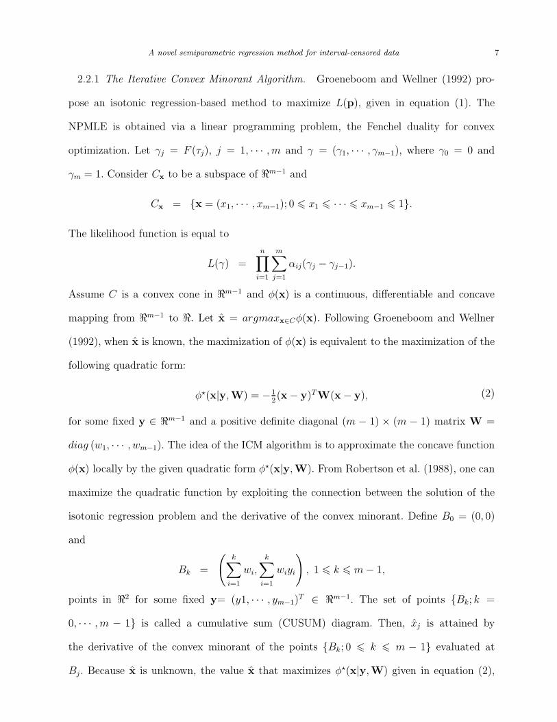
2.2.1 The Iterative Convex Minorant Algorithm. Groeneboom and Wellner (1992) pro-

pose an isotonic regression-based method to maximize L(p), given in equation (1). The

NPMLE is obtained via a linear programming problem, the Fenchel duality for convex

optimization. Let γj = F (τj), j = 1, · · · , m and γ = (γ1, · · · , γm−1), where γ0 = 0 and

γm = 1. Consider Cx

to be a subspace of ℜm−1 and

Cx

= {x = (x1, · · · , xm−1); 0 6 x1 6 · · · 6 xm−1 6 1}.

The likelihood function is equal to

L(γ) =

n∏

i=1

m∑

j=1

αij(γj − γj−1).

Assume C is a convex cone in ℜm−1 and φ(x) is a continuous, differentiable and concave

mapping from ℜm−1 to ℜ. Let x = argmaxx∈Cφ(x). Following Groeneboom and Wellner

(1992), when x is known, the maximization of φ(x) is equivalent to the maximization of the

following quadratic form:

φ⋆(x|y,W) = −12(x − y)TW(x− y), (2)

for some fixed y ∈ ℜm−1 and a positive definite diagonal (m − 1) × (m − 1) matrix W =

diag (w1, · · · , wm−1). The idea of the ICM algorithm is to approximate the concave function

φ(x) locally by the given quadratic form φ⋆(x|y,W). From Robertson et al. (1988), one can

maximize the quadratic function by exploiting the connection between the solution of the

isotonic regression problem and the derivative of the convex minorant. Define B0 = (0, 0)

and

Bk =

(k∑

i=1

wi,k∑

i=1

wiyi

), 1 6 k 6 m − 1,

points in ℜ2 for some fixed y= (y1, · · · , ym−1)T ∈ ℜm−1. The set of points {Bk; k =

0, · · · , m − 1} is called a cumulative sum (CUSUM) diagram. Then, xj is attained by

the derivative of the convex minorant of the points {Bk; 0 6 k 6 m − 1} evaluated at

Bj. Because x is unknown, the value x that maximizes φ⋆(x|y,W) given in equation (2),

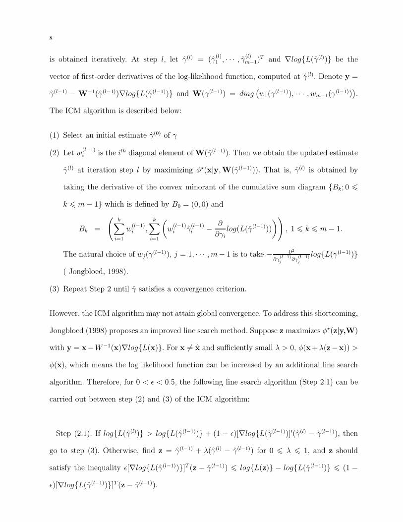
8

is obtained iteratively. At step l, let γ(l) = (γ(l)1 , · · · , γ

(l)m−1)

T and ∇log{L(γ(l))} be the

vector of first-order derivatives of the log-likelihood function, computed at γ(l). Denote y =

γ(l−1) − W−1(γ(l−1))∇log{L(γ(l−1))} and W(γ(l−1)) = diag(w1(γ

(l−1)), · · · , wm−1(γ(l−1))

).

The ICM algorithm is described below:

(1) Select an initial estimate γ(0) of γ

(2) Let w(l−1)i is the ith diagonal element of W(γ(l−1)). Then we obtain the updated estimate

γ(l) at iteration step l by maximizing φ⋆(x|y,W(γ(l−1))). That is, γ(l) is obtained by

taking the derivative of the convex minorant of the cumulative sum diagram {Bk; 0 6

k 6 m − 1} which is defined by B0 = (0, 0) and

Bk =

(k∑

i=1

w(l−1)i ,

k∑

i=1

(w

(l−1)i γ

(l−1)i −

∂

∂γi

log(L(γ(l−1)))

)), 1 6 k 6 m − 1.

The natural choice of wj(γ(l−1)), j = 1, · · · , m− 1 is to take − ∂2

∂γ(l−1)j ∂γ

(l−1)j

log{L(γ(l−1))}

( Jongbloed, 1998).

(3) Repeat Step 2 until γ satisfies a convergence criterion.

However, the ICM algorithm may not attain global convergence. To address this shortcoming,

Jongbloed (1998) proposes an improved line search method. Suppose z maximizes φ⋆(z|y,W)

with y = x−W−1(x)∇log{L(x)}. For x 6= x and sufficiently small λ > 0, φ(x+λ(z−x)) >

φ(x), which means the log likelihood function can be increased by an additional line search

algorithm. Therefore, for 0 < ǫ < 0.5, the following line search algorithm (Step 2.1) can be

carried out between step (2) and (3) of the ICM algorithm:

Step (2.1). If log{L(γ(l))} > log{L(γ(l−1))} + (1 − ǫ)[∇log{L(γ(l−1))]′(γ(l) − γ(l−1)), then

go to step (3). Otherwise, find z = γ(l−1) + λ(γ(l) − γ(l−1)) for 0 6 λ 6 1, and z should

satisfy the inequality ǫ[∇log{L(γ(l−1))}]T (z − γ(l−1)) 6 log{L(z)} − log{L(γ(l−1))} 6 (1 −

ǫ)[∇log{L(γ(l−1))}]T (z− γ(l−1)).


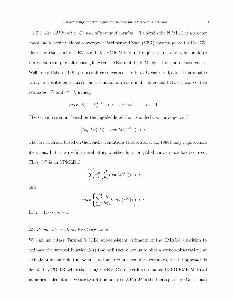
2.2.2 The EM Iterative Convex Minorant Algorithm. To obtain the NPMLE at a greater

speed and to achieve global convergence, Wellner and Zhan (1997) have proposed the EMICM

algorithm that combines EM and ICM. EMICM does not require a line search, but updates

the estimates of p by alternating between the EM and the ICM algorithms, until convergence.

Wellner and Zhan (1997) propose three convergence criteria. Given ǫ > 0, a fixed permissible

error, first criterion is based on the maximum coordinate difference between consecutive

estimates γ(l) and γ(l−1), namely

maxj

∣∣∣γ(l)j − γ

(l−1)j

∣∣∣ < ǫ, for j = 1, · · · , m − 1.

The second criterion, based on the log-likelihood function, declares convergence if

∣∣log(L(γ(l))) − log(L(γ(l−1)))∣∣ < ǫ.

The last criterion, based on the Fenchel conditions (Robertson et al., 1988), may require more

iterations, but it is useful in evaluating whether local or global convergence has occurred.

Thus, γ(l) is an NPMLE if∣∣∣∣∣m−1∑

j=1

γ(l)j

∂

∂γj

log(L(γ(l)))

∣∣∣∣∣ < ǫ,

and

max

{m−1∑

k=j

∂

∂γk

log(L(γ(l)))

}< ǫ,

for j = 1, · · · , m − 1.

2.3 Pseudo-observations-based regression

We can use either Turnbull’s (TB) self-consistent estimator or the EMICM algorithm to

estimate the survival function S(t) that will then allow us to obtain pseudo-observations at

a single or at multiple timepoints. In simulated and real data examples, the TB approach is

denoted by PO-TB, while that using the EMICM algorithm is denoted by PO-EMICM. In all

numerical calculations, we use two R functions: (i) EMICM in the Icens package (Gentleman

10

and Vandal, 2009) for EMICM algorithm and (ii) geese from the geepack package (Yan,

2002) for GEE implementation.

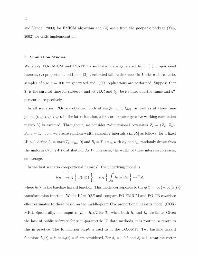
3. Simulation Studies

We apply PO-EMICM and PO-TB to simulated data generated from: (1) proportional

hazards, (2) proportional odds and (3) accelerated failure time models. Under each scenario,

samples of size n = 100 are generated and 1, 000 replications are performed. Suppose that

Ti is the survival time for subject i and let IQR and t(q) be its inter-quartile range and qth

percentile, respectively.

In all scenarios, POs are obtained both at single point t(50), as well as at three time

points (t(45), t(50), t(55)). In the later situation, a first-order autoregressive working correlation

matrix Vi is assumed. Throughout, we consider 2-dimensional covariates Zi = (Zi1, Zi2).

For i = 1, . . . , n, we create random-width censoring intervals (Li, Ri] as follows: for a fixed

W > 0, define Li = max(Ti−ciL, 0) and Ri = Ti+ciR, with ciL and ciR randomly drawn from

the uniform U(0, 2W ) distribution. As W increases, the width of these intervals increases,

on average.

In the first scenario (proportional hazards), the underlying model is

log

[−log

{S(t|Z)

}]= log

{ ∫ t

0

h0(u)du

}−βT Z,

where h0(·) is the baseline hazard function. This model corresponds to the g(t) = log{−log(S(t)}

transformation function. We fix W = IQR and compare PO-EMICM and PO-TB covariate

effect estimates to those based on the middle-point Cox proportional hazards model (COX-

MPI). Specifically, one imputes (Li + Ri)/2 for Ti, when both Ri and Li are finite. Given

the lack of public software for semi-parametric IC data methods, it is routine to resort to

this in practice. The R function coxph is used to fit the COX-MPI. Two baseline hazard

functions h0(t) = t3 or h0(t) = t4 are considered. For β1 = −0.5 and β2 = 1, covariate vector


Zi = (Zi1, Zi2) is such that Zi1 and Zi2 are independent, Bernoulli(0.5) and N(3, σ2 = 0.5)-

distributed, respectively. Summary results presented in Table 1 include: the empirical mean

of the β estimates, the average of the estimated β standard errors, the empirical standard

error of the β estimates and the coverage probability of the true β by the nominal 95%

confidence intervals.

[Table 1 about here.]

PO-EMICM and PO-TB perform very well in all scenarios, producing virtually unbiased

estimators for (β1, β2), with appropriate coverage probabilities. Resulting parameter esti-

mates when POs are obtained at multiple timepoints are more efficient than their single-

point counterparts. PO-EMICM appears to be more efficient than PO-TB, mainly due to the

benefits conferred by the ICM algorithm. Although more efficient, since it uses information

across the entire survival curve, the middle-point imputation approach, COX-MPI, produces

substantially biased β1 and β2 estimates, fact also reflected in the coverage probabilities

below the nominal level.

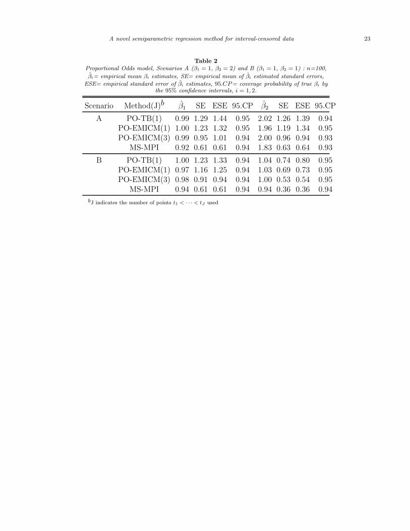
The second simulation set is devised for the proportional odds model

logit

{S(t|Z)

}= logit

{S0(t)

}−βT Z,

with baseline survival function S0(t). The appropriate link function is obviously g(t) =

logit(t). We let S0(t) = e−t, W = 0.3IQR, and generate Zi = (Zi1, Zi2) as follows: for

(β1, β2) = (1, 2), we generate Zi1 and Zi2 from independent uniform U(1, 2) and U(2, 3)

distributions, respectively; when (β1, β2) = (1, 1), Zi1 and Zi2 are generated independently

from U(1, 2) and Bernoulli(0.5) distributions, respectively. For comparison, we also employ

the method developed by Martinussen and Scheike (2006) for right-censored data obeying

a proportional odds model. As such, for all finite intervals (Li, Ri], we resort once more to

middle-point imputation and present our results under MS-MPI. This method is implemented

using the R function prop.odds in the timereg (Scheike et al., 2009) package. Results shown

12

in Table 2, indicate that the proposed PO-EMICM and PO-TB methods perform very well,

in terms of bias and coverage probabilities. MS-MPI appears to underestimate both β1 and

β2, while being more efficient.


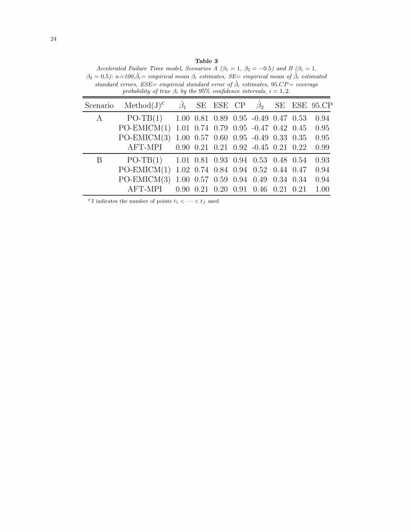
The third simulation study is designed for a particular accelerated failure time model

T = exp(β1Zi1 + β2Zi2 + U),

where exp(U) follows the Gompertz(1, 1) distribution. The conditional survival function

S(t|Zi) follows the model

S(t|Zi) = exp

[1 − exp

{te−(β1Zi1+β2Zi2)

}].

Thus, the transformation function is g(t) = log[log{1−log(t)}]. We let W = IQR/2 and gen-

erate data as follows: when (β1, β2) = (1,−0.5), Zi1 and Zi2 are generated independently from

U(2, 3) and Bernoulli(0.5) distributions, respectively; when (β1, β2) = (1, 0.5), we generate

Zi1 and Zi2 independently from U(2, 3) and N(2, σ2 = 0.5), respectively. For comparison, we

use a parametric accelerated failure time model based on the middle point imputations

(AFT-MPI). To implement the parametric approach, we use the function survreg from

the R package survival (Therneau and Lumley, 2009) and assume a Weibull distribution.

Simulation results displayed in Table 3 indicate that both PO-EMICM and PO-TB produce

good estimates of β1 and β2, and the 95% confidence intervals’ coverage probabilities are

very close to the nominal level. On the other hand, AFT-MPI produces biased parameter

estimates in all scenarios.


4. The IBCSG Trial VI Study

Breast cancer is one of the most common types of cancer in the United States. Bonadonna

et al. (1976) has proposed a prolonged cyclic adjuvant chemotherapy for breast cancer,


showing that a 12-month postoperative combination chemotherapy of cyclophosphamide,

methotrexate and fluorouracil (CMF) is associated with a decreased risk of breast cancer

recurrence of in women with positive axillary lymph nodes. The International Breast Cancer

Study Group (IBCSG) Trial VI has investigated the optimal duration and timing of this

combination chemotherapy.

Of interest was how CMF, with or without subsequent re-introduction, is associated with

time to breast cancer recurrence, as well as overall survival. Between July 1986 to April 1993,

eligible patients were randomly assigned, with equal probability, to one of the following four

regimens: (i) CMF for six initial consecutive courses on months 1-6 (CMF6); (ii) CMF for six

initial consecutive courses on months 1-6 plus three single courses of re-introduction CMF

given on months 9, 12, 15 (CMF6+3); (iii) CMF for three initial consecutive courses on

month 1-3 (CMF3) and (iv) CMF for three initial consecutive courses on months 1-3 plus

three single courses of re-introduction CMF given on months 6, 9, 12 (CMF3+3).

Based on repeated clinic visits, recurrence time was assessed as the difference between

the randomization date and the relapse date, defined as the visit when cancer relapse was

established. The inter-visit average duration was 6.9 months, thus pinning down the precise

time of cancer recurrence is problematic. Conceivably, cancer relapse does not occur exactly

at the visit time when it is established, but sometime before that. Therefore, it might be more

appropriate to treat the time-to-relapse as an interval-censored event occurring between the

visit when recurrent disease was established and the last cancer-free visit. Accordingly, we

model disease free survival (DFS) time as interval-censored data. To compare DFS under

the four CMF regimens, we assume an underlying proportional hazards model. It is well-

established (see International Breast Cancer Study Group (1996) and Gruber et al. (2008))

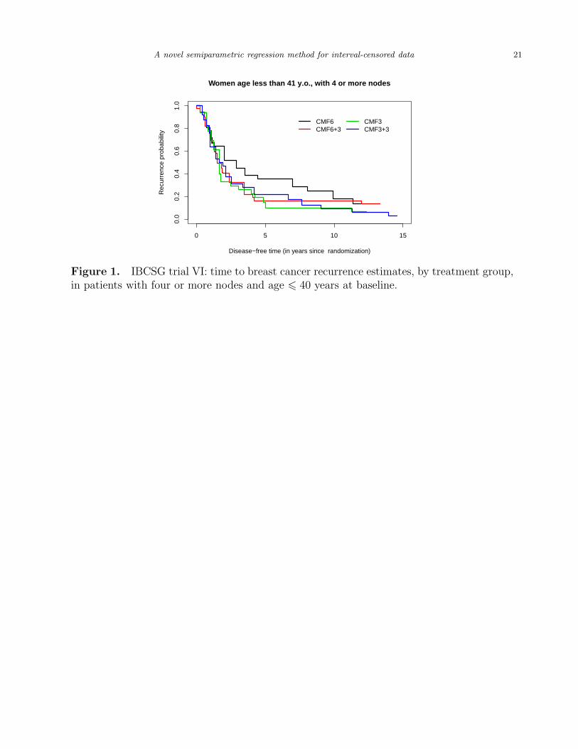
that patient age at baseline and node group are significantly associated with DFS. We focus

attention on the group of 131 women age 41 years or younger at baseline, with four or more

14

cancer nodules. Figure 1 depicts the DFS estimates in the four groups obtained based on

the EMICM algorithm. The highest risk of relapse is associated with CMF3, while the best

prognosis is for patients receiving the standard CMF6 regimen.

To compare the four CMF regimens, we present unadjusted, as well as adjusted models.

Adjustment factors are: tumor grade (1 (reduced), 2, 3(increased)), tumor size (6 2 vs.

> 2 cm across), vessel invasion (yes/no), estrogen receptor (ER) status (negative/positive),

progesterone receptor (PR) status (negative/positive).

We present least squares estimates when the POs used in PO-EMICM are computed

only at the median timepoint 1.75. When POs computed at three timepoints (1.65, 1.75

and 1.98, representing the 45th, 50th and 55th percentiles of the EMICM-based relapse time

distribution estimator), we employ GEEs with a first-order autoregressive working correlation

matrix. In addition, employ the middle-point imputation approach (COX-MPI) described in

simulations, thus replacing the interval-censored with a right-censored data structure. Results

presented in Table 4 include the hazard ratio (HR) estimates, together with corresponding

95% confidence intervals and p-values (P).

[Figure 1 about here.]


Analyses employing the two POs-based method, labeled PO-EMICM(1) and PO-EMICM(3)

reveal some interesting findings. Mortality in the CMF3 arm is significantly higher than in the

CMF6 (reference) group, both in adjusted and unadjusted models. Importantly, in adjusted

models, the estimated hazard rate in more than twice as high in the CMF3 group, compared

to the CMF6 standard regimen (HR=2.18 (p-value=0.006) in PO-EMICM(1) and HR=2.37

(p-value=0.009) in EM-ICM(3)). Using the middle-point imputation strategy (COX-MPI), in

which data are treated as right-censored, no significant differences are found between CMF6

and any of the other three regimens. For example, the estimated hazard ration for CMF3 in


the adjusted model is equal to 1.93 (p-value of 0.054), thus not significantly different from

1 at a 5% significance level. In conclusion, recognizing the true nature of the data (interval-

censored, in this case) is important and can have major implications. Although convenient,

the practice of imputing the middle point and then treating the data as right-censored, may

lead to biased results or, as seen here, to a lack of statistical significance.

5. Discussion

This article presents a novel, PO-based regression method, for modeling interval-censored

event times. Many existing nonparametric or semiparametric methods for IC data do not

seem to be used routinely, likely due to a lack of software availability. The proposed method

is computationally simple, thus convenient to implement using standard software. POs

are constructed using an NPMLE of the survival function. Because the NPMLE does not

have a closed-form in interval-censored data, two iterative algorithms (Turnbull’s method

and EMICM) are used in this methodological development. However, we emphasize an

important distinction. Existing estimation and testing methods for interval-censored data

usually employ EM-type algorithms to estimate covariate effects, with inherited potential

problems, such as local convergence or lack thereof. Henschel et al. (2007) have indicated

similar problems with algorithm convergence. By contrast, our PO-based approach leads

to covariate effect estimates that are obtained in a direct fashion, using GEE or least-

squares regression. Iteration is only required to estimate the survival function and EMICM

guarantees global convergence to the NPMLE. Furthermore, using our approach, robust

variance estimates are readily available, thus facilitating significance testing and confidence

intervals construction. Importantly, model misspecification will lead to biases covariate effect

estimates. For example, if the true underlying model obeys proportional hazards, yet the

fitted model assumed proportional odds, the resulting parameter estimates will be incorrect,

although their statistical significance may be preserved.

16

Acknowledgments

The authors would like to thank the IBCSG for permission to use their data. ACA’s re-

search is supported in part by following grants: P30 CA014520-36, UL1 RR025011-03, R21

CA132267-02 and W81XWH-08-1-0341. KWT’s research is supported in part by the NSF

grant DMS-0604931.

References

Alioum, A. and Commenges, D. (1996). A proportional hazards model for arbitrarily censored

and truncated data. Biometrics 52, 512–524.

Andersen, P. K., Hansen, M. G., and Klein, J. P. (2004). Regression analysis of restricted

mean survival time based on pseudo-observations. Life Time Data Analysis 10, 335–350.

Andersen, P. K. and Klein, J. P. (2007). Regression analysis for multistate models based

on a pseudo-value approach with applications to bone marrow transplantation studies.

Scandinavian Journal of Statistics 34, 3–16.

Andersen, P. K., Klein, J. P., and Rosthφj, S. (2003). Generalized linear models for correlated

pseudo-observations, with applications to multi-state models. Biometrika 90, 15–27.

Andrei, A. C. and Murray, S. (2007). Regression models for the mean of quality-of-life-

adjusted restricted survival time using pseudo-observations. Biometrics 63, 398–404.

Betensky, R. A., Lindsey, J. C., Ryan, L. M., and Wand, M. P. (2002). A local likelihood

proportional hazards model for interval censored data. Statistics in Medicine 21, 263–

275.

Betensky, R. A., Rabinowitz, D., and Tsiatis, A. A. (2001). Computationally simple

accelerated failure time regression for interval censored data. Biometrika 88, 703–711.

Bohning, D., Schlattmann, P., and Dietz, E. (1996). Interval censored data: A note on the

nonparametric maximum likelihood estimator of the distribution function. Biometrika

83, 462–466.


Bonadonna, G., Brusamolino, E., Valagussa, P., and et al. (1976). Combination chemother-

apy as an adjuvant treatment in operable breast cancer. New England Journal of

Medicine 294, 405–410.

Braun, J., Duchesne, T., and Stafford, J. E. (2005). Local likelihood density estimation for

interval censored data. The Canadian Journal of Statistics 33, 39–60.

Cai, T. and Betensky, R. A. (2003). Hazard regression for interval-censored data with

penalized spline. Biometrics 59, 570–579.

Finkelstein, D. M. (1986). A proportional hazards model for interval censored failure time

data. Biometrics 42, 845–854.

Gentleman, R. and Vandal, A. (2009). Icens: NPMLE for Censored and Truncated Data. R

package version 1.2.0.

Gentlemen, R. and Geyer, C. J. (1994). Maximum likelihood for interval censored data:

Consistency and computation. Biometrika 81, 618–623.

Goodall, R. L., Dunn, D. T., and Babiker, A. G. (2004). Interval–censored survival time

data: confidence intervals for the nonparametric survivor function. Statistics in Medicine

23, 1131–1145.

Graw, F., Gerds, T. A., and Schumacher, M. (2009). On pseudo-values for regression analysis

in competing risks models. Lifetime Data Analysis 15, 241–255.

Groeneboom, P. and Wellner, J. A. (1992). Information bounds and non–parametric

maximum likelihood. DMV seminar, Band 19, Birkhauser, New York.

Gruber, G., Cole, B. F., Castinglione-Gertsch, M., and et al. (2008). Extracapsular tumor

spread and the risk of local, axillary and supraclavicular recurrence in node-positive,

premenopausal patients with breast cancer. Annals of Oncology 19, 1393–1401.

Henschel, V., Heiß, C., and Mansmann, U. (2007). intcox: Iterated Convex Minorant

Algorithm for interval censored event data. R package version 0.9.1.1.

18

Hudgens, M. G. (2005). On nonparametric maximum likelihood estimation with interval

censoring and left truncation. Journal of the Royal Statistical Society, Series B 67,

573–587.

International Breast Cancer Study Group (1996). Duration and reintroduction of adjuvant

chemotherapy for node-positive premenopausal breast cancer patients. Journal of

Clinical Oncology 14, 1885–1894.

Jongbloed, G. (1998). The iterative convex minorant algorithm for nonparametric estimation.

Journal of Computational & Graphical Statistics 7, 310–321.

Klein, J. P. and Andersen, P. K. (2005). Regression modeling for competing risks data based

on pseudo-values of the cumulative incidence function. Biometrics 61, 223–229.

Li, L. and Pu, Z. (2003). Rank estimation of log-linear regression with interval censored

data. Lifetime Data Analysis 9, 57–70.

Li, L., Watkins, T., and Yu, Q. (1997). An EM algorithm for smoothing the self-consistent

estimator of survival functions with interval-censored data. Scandinavian Journal of

Statistics 24, 531–542.

Lindsey, J. C. and Ryan, L. M. (1998). Tutorial in biostatistics methods for interval-censored

data. Statistics in Medicine 17, 219–238.

Liu, L., Logan, B. R., and Klein, J. P. (2008). Inference for current leukemia free survival.

Lifetime data analysis 14, 432–446.

Logan, B. R., Nelson, G. O., and Klein, J. P. (2008). Analyzing center specific outcomes in

hematopoietic cell transplantation. Lifetime data analysis 14, 389–404.

Martinussen, T. and Scheike, T. (2006). Dynamic Regression Models for Survival Data.

Springer Verlag.

Murphy, S. A., Rossini, A. J., and van der Vaart, A. W. (1997). Maximum likelihood esti-

mation in the proportional odds model. Journal of the American Statistical Association


92, 968–976.

Pan, W. and Chappell, R. (1998). Estimating survival curves with left truncated and

interval censored data via the EMS algorithm. Communications in Statistics. Theory

and Methods 27, 777–793.

Quenouille, M. (1949). Approximate tests of correlation in time series. Journal of the Royal

Statistical Society, Series B 11, 18–84.

Rabinowitz, D., Betensky, R. A., and Tsiatis, A. A. (2000). Using conditional logistic

regression to fit proportional odds models to interval censored data. Biometrics 56,

511–518.

Robertson, T., Wright, F. T., and Dykstra, R. L. (1988). Order Restricted Statistical

Inference. John Wiley: New York.

Satten, G. A. (1996). Rank-based inference in the proportional hazards model for interval

censored data. Biometrika 83, 355–370.

Scheike, T., Martinussen, T., and Silver, J. (2009). timereg: timereg package for flexible

regression models for survival data. R package version 1.2-5.

Scheike, T. and Zhang, M. J. (2007). Direct modelling of regression effects for transition

probabilities in multistate models. Scandinavian Journal of Statistics 34, 17–32.

Shen, X. (1998). Proportional odds regression and sieve maximum likelihood estimation.

Biometrika 85, 165–177.

Simonoff, J. S. and Tsai, C. L. (1986). Jacknife-based estimators and confidence regions in

nonlinear regression. Technometrics 28, 103–112.

Sun, J. (2006). The statistical analysis of interval-censored failure time data. Springer-Verlag:

New York.

Sun, J., Sun, L., and Zhu, C. (2007). Testing the proportional odds model for interval-

censored data. Lifetime Data Analysis 13, 37–50.

20

Therneau, T. and Lumley, T. (2009). survival: Survival analysis, including penalised

likelihood. R package version 2.35-7.

Tian, L. and Cai, T. (2006). On the accelerated failure time model for current status and

interval censored data. Biometrika 93, 329–342.

Tukey, J. W. (1958). Bias and confidence in not quite large samples. Annals of Mathematical

Statistics 29, 614.

Turnbull, B. W. (1976). The empirical distribution function with arbitrarily grouped

censored and truncated data. Journal of the Royal Statistical Society, Series B 38,

290–295.

Wellner, J. A. and Zhan, Y. (1997). A hybrid algorithm for computation of the nonparametric

maximum likelihood estimator from censored data. Journal of the American Statistical

Association 92, 945–959.

Wu, C. F. J. (1986). Jackknife,bootstrap and other resampling methods in regression

analysis. Annals of Statistics 14, 1261–1295.

Xue, H., Lam, K. F., Ben, C., and De Wolf, F. (2006). Semiparametric accelerated failure

time regression analysis with application to interval-censored HIV/AIDS data. Statistics

in Medicine 25, 3850–3863.

Yan, J. (2002). geepack: Yet another package for generalized estimating equations. R-News

pages 12–14.


0 5 10 15

0.0

0.2

0.4

0.6

0.8

1.0

Disease−free time (in years since randomization)

Rec

urre

nce

prob

abili

ty

Women age less than 41 y.o., with 4 or more nodes

CMF6CMF6+3

CMF3CMF3+3

Figure 1. IBCSG trial VI: time to breast cancer recurrence estimates, by treatment group,in patients with four or more nodes and age 6 40 years at baseline.

22

Table 1

Proportional Hazards model, Scenarios A (h0(t) = t3) and B (h0(t) = t4): n = 100,

β1 = −0.5, β2 = 1.0, h0(t) =baseline hazard, βi= empirical mean βi estimates, SE=

empirical mean of βi estimated standard errors, ESE= empirical standard error of βi

estimates, 95.CP= coverage probability of true βi by the 95% confidence intervals, i = 1, 2.

Scenario Method(J)a β1 SE ESE 95.CP β2 SE ESE 95.CP

A PO-TB(1) -0.52 0.83 0.92 0.95 1.05 0.79 0.89 0.93PO-EMICM(1) -0.50 0.76 0.81 0.95 1.04 0.76 0.83 0.95PO-EMICM(3) -0.52 0.61 0.62 0.95 1.01 0.58 0.62 0.94

COX-MPI -0.42 0.21 0.22 0.92 0.83 0.23 0.22 0.85

B PO-TB(1) -0.55 0.82 0.87 0.95 1.05 0.76 0.87 0.94PO-EMICM(1) -0.51 0.76 0.81 0.95 1.04 0.76 0.82 0.96PO-EMICM(3) -0.52 0.61 0.63 0.94 1.01 0.57 0.61 0.93

COX-MPI -0.41 0.21 0.22 0.91 0.82 0.22 0.22 0.84aJ indicates the number of points t1 < · · · < tJ used


Table 2

Proportional Odds model, Scenarios A (β1 = 1, β2 = 2) and B (β1 = 1, β2 = 1) : n=100,

βi= empirical mean βi estimates, SE= empirical mean of βi estimated standard errors,

ESE= empirical standard error of βi estimates, 95.CP= coverage probability of true βi bythe 95% confidence intervals, i = 1, 2.

Scenario Method(J)b β1 SE ESE 95.CP β2 SE ESE 95.CP

A PO-TB(1) 0.99 1.29 1.44 0.95 2.02 1.26 1.39 0.94PO-EMICM(1) 1.00 1.23 1.32 0.95 1.96 1.19 1.34 0.95PO-EMICM(3) 0.99 0.95 1.01 0.94 2.00 0.96 0.94 0.93

MS-MPI 0.92 0.61 0.61 0.94 1.83 0.63 0.64 0.93

B PO-TB(1) 1.00 1.23 1.33 0.94 1.04 0.74 0.80 0.95PO-EMICM(1) 0.97 1.16 1.25 0.94 1.03 0.69 0.73 0.95PO-EMICM(3) 0.98 0.91 0.94 0.94 1.00 0.53 0.54 0.95

MS-MPI 0.94 0.61 0.61 0.94 0.94 0.36 0.36 0.94

bJ indicates the number of points t1 < · · · < tJ used

24

Table 3

Accelerated Failure Time model, Scenarios A (β1 = 1, β2 = −0.5) and B (β1 = 1,

β2 = 0.5): n=100,βi= empirical mean βi estimates, SE= empirical mean of βi estimated

standard errors, ESE= empirical standard error of βi estimates, 95.CP= coverageprobability of true βi by the 95% confidence intervals, i = 1, 2.

Scenario Method(J)c β1 SE ESE CP β2 SE ESE 95.CP

A PO-TB(1) 1.00 0.81 0.89 0.95 -0.49 0.47 0.53 0.94PO-EMICM(1) 1.01 0.74 0.79 0.95 -0.47 0.42 0.45 0.95PO-EMICM(3) 1.00 0.57 0.60 0.95 -0.49 0.33 0.35 0.95

AFT-MPI 0.90 0.21 0.21 0.92 -0.45 0.21 0.22 0.99

B PO-TB(1) 1.01 0.81 0.93 0.94 0.53 0.48 0.54 0.93PO-EMICM(1) 1.02 0.74 0.84 0.94 0.52 0.44 0.47 0.94PO-EMICM(3) 1.00 0.57 0.59 0.94 0.49 0.34 0.34 0.94

AFT-MPI 0.90 0.21 0.20 0.91 0.46 0.21 0.21 1.00cJ indicates the number of points t1 < · · · < tJ used


Table 4

The International Breast Cancer Study Group Trial VI example: patients with four or morenodes and age 6 40 years at baseline.

Model type Unadjusted Adjusted

Interval-Censored (PO-EMICM(1)) HR 95 % CI P HR 95 % CI P

CMF6 1.00 reference 1.00 referenceCMF6+3 1.22 0.64-2.33 0.56 1.62 0.90-2.91 0.11CMF3 1.65 0.93-2.91 0.09 2.18 1.26-3.78 0.006

CMF3+3 1.48 0.84-2.61 0.18 1.25 0.59-2.62 0.57

Interval-Censored (PO-EMICM(3))


CMF3+3 1.24 0.61-2.53 0.546 1.15 0.53-2.52 0.714

Right-Censored (Cox Model MPI)


CMF3+3 1.43 0.85-2.40 0.184 1.05 0.54-2.05 0.894

Documents

UNIVERSITY OF WISCONSIN DEPARTMENT OF ... OF WISCONSIN DEPARTMENT OF BIOSTATISTICS AND MEDICAL INFORMATICS UNIVERSITY OF WISCONSIN DEPARTMENT OF BIOSTATISTICS AND MEDICAL INFORMATICS