Embed Size (px)
Citation preview
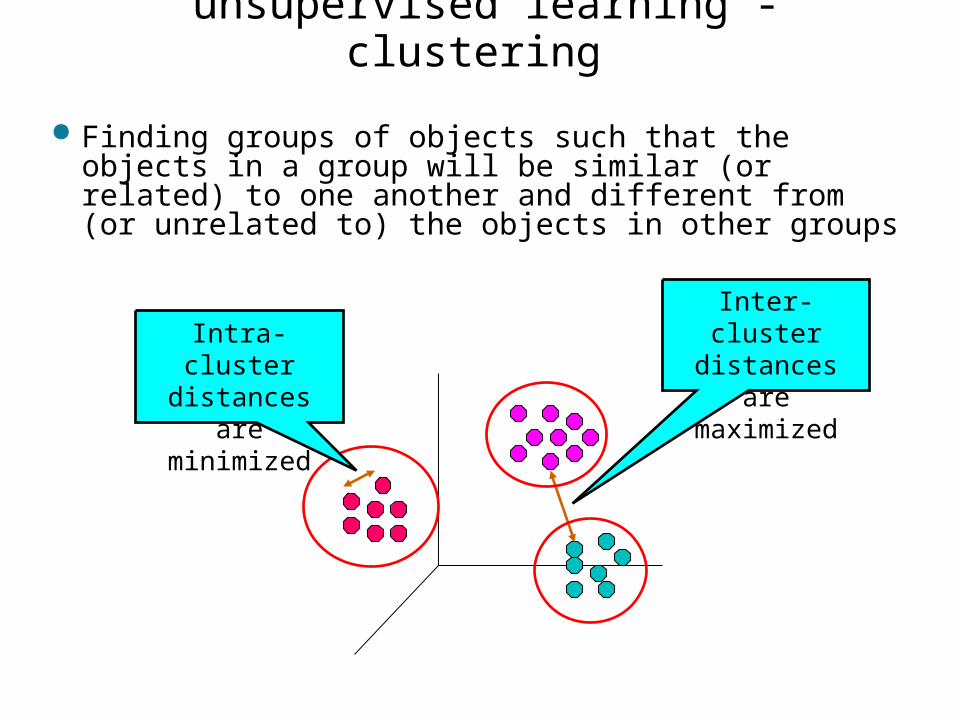
unsupervised learning - clustering
Finding groups of objects such that the objects in a group will be similar (or related) to one another and different from (or unrelated to) the objects in other groups
Inter-cluster distances are maximized
Intra-cluster distances are
minimized
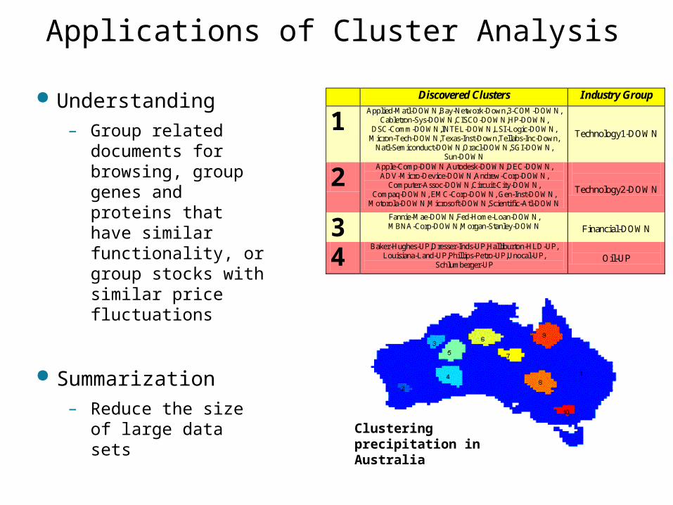
Applications of Cluster Analysis
Understanding– Group related
documents for browsing, group genes and proteins that have similar functionality, or group stocks with similar price fluctuations
Summarization– Reduce the size of
large data sets
Discovered Clusters Industry Group
1 Applied-Matl-DOWN,Bay-Network-Down,3-COM-DOWN,
Cabletron-Sys-DOWN,CISCO-DOWN,HP-DOWN, DSC-Comm-DOWN,INTEL-DOWN,LSI-Logic-DOWN,
Micron-Tech-DOWN,Texas-Inst-Down,Tellabs-Inc-Down, Natl-Semiconduct-DOWN,Oracl-DOWN,SGI-DOWN,
Sun-DOWN
Technology1-DOWN
2 Apple-Comp-DOWN,Autodesk-DOWN,DEC-DOWN,
ADV-Micro-Device-DOWN,Andrew-Corp-DOWN, Computer-Assoc-DOWN,Circuit-City-DOWN,
Compaq-DOWN, EMC-Corp-DOWN, Gen-Inst-DOWN, Motorola-DOWN,Microsoft-DOWN,Scientific-Atl-DOWN
Technology2-DOWN
3 Fannie-Mae-DOWN,Fed-Home-Loan-DOWN, MBNA-Corp-DOWN,Morgan-Stanley-DOWN
Financial-DOWN
4 Baker-Hughes-UP,Dresser-Inds-UP,Halliburton-HLD-UP,
Louisiana-Land-UP,Phillips-Petro-UP,Unocal-UP, Schlumberger-UP
Oil-UP
Clustering precipitation in Australia
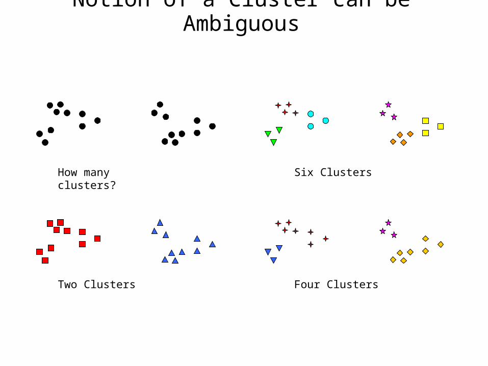
Notion of a Cluster can be Ambiguous
How many clusters?
Four Clusters Two Clusters
Six Clusters
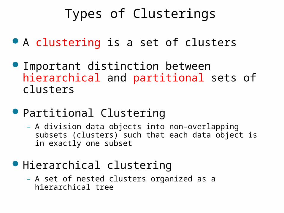
Types of Clusterings
A clustering is a set of clusters
Important distinction between hierarchical and partitional sets of clusters
Partitional Clustering– A division data objects into non-overlapping subsets
(clusters) such that each data object is in exactly one subset
Hierarchical clustering– A set of nested clusters organized as a hierarchical tree
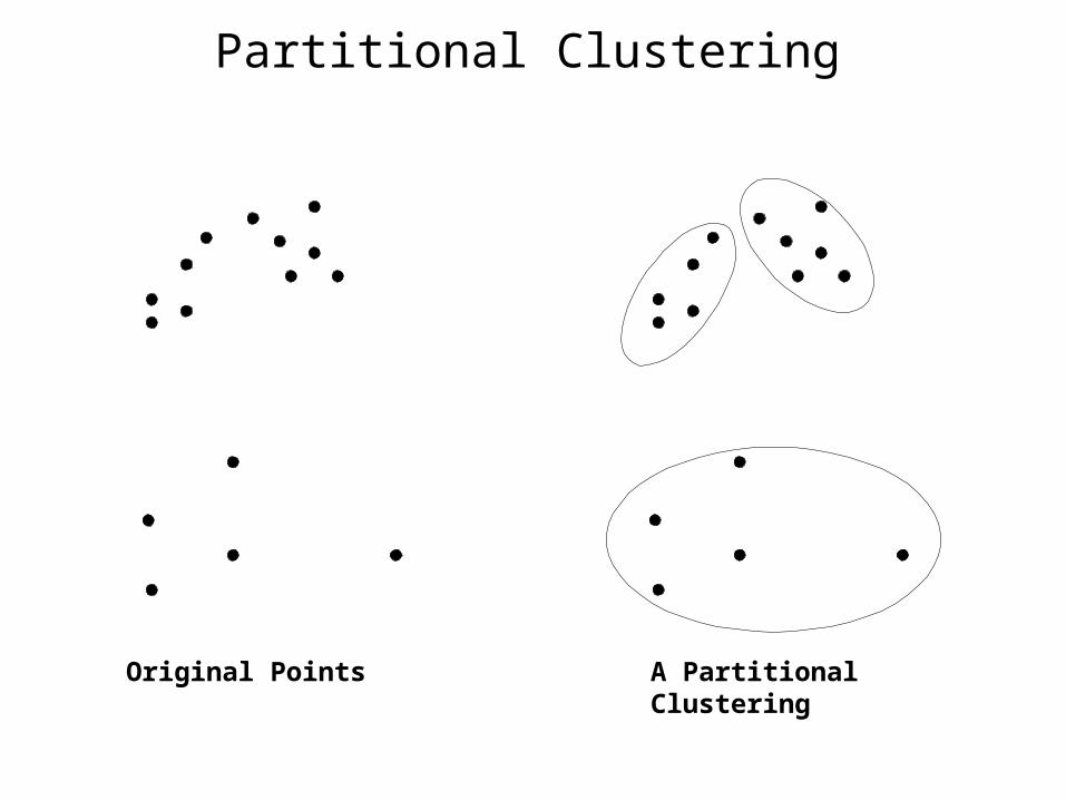
Partitional Clustering
Original Points A Partitional Clustering
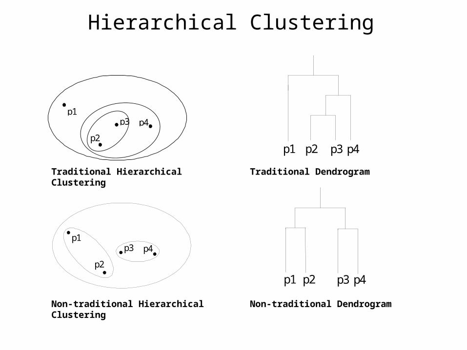
Hierarchical Clustering
p4p1
p3
p2
p4 p1
p3
p2
p4p1 p2 p3
p4p1 p2 p3
Traditional Hierarchical Clustering
Non-traditional Hierarchical Clustering
Non-traditional Dendrogram
Traditional Dendrogram
Clustering Algorithms
K-means and its variants
Hierarchical clustering
Density-based clustering
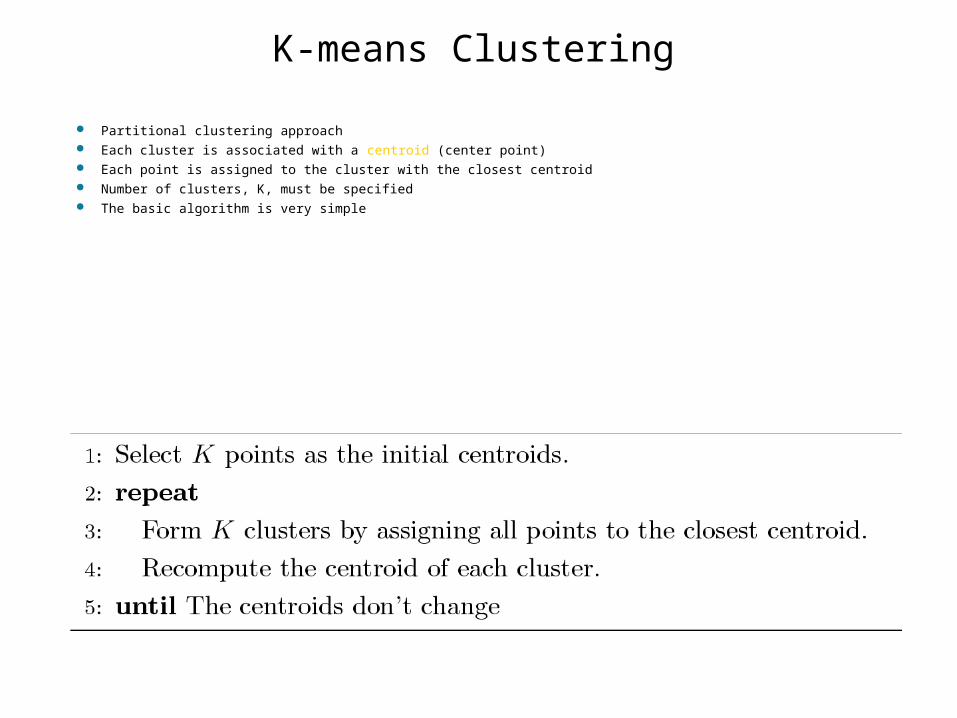
K-means Clustering
Partitional clustering approach Each cluster is associated with a centroid (center point) Each point is assigned to the cluster with the closest centroid Number of clusters, K, must be specified The basic algorithm is very simple
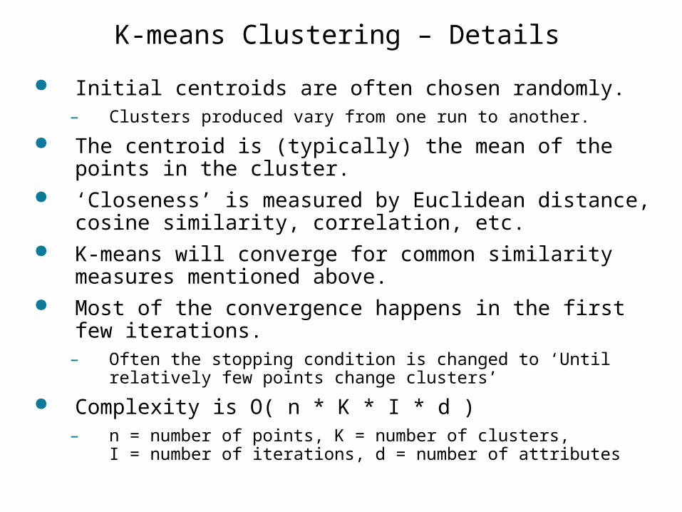
K-means Clustering – Details
Initial centroids are often chosen randomly.– Clusters produced vary from one run to another.
The centroid is (typically) the mean of the points in the cluster.
‘Closeness’ is measured by Euclidean distance, cosine similarity, correlation, etc.
K-means will converge for common similarity measures mentioned above.
Most of the convergence happens in the first few iterations.
– Often the stopping condition is changed to ‘Until relatively few points change clusters’
Complexity is O( n * K * I * d )– n = number of points, K = number of clusters,
I = number of iterations, d = number of attributes
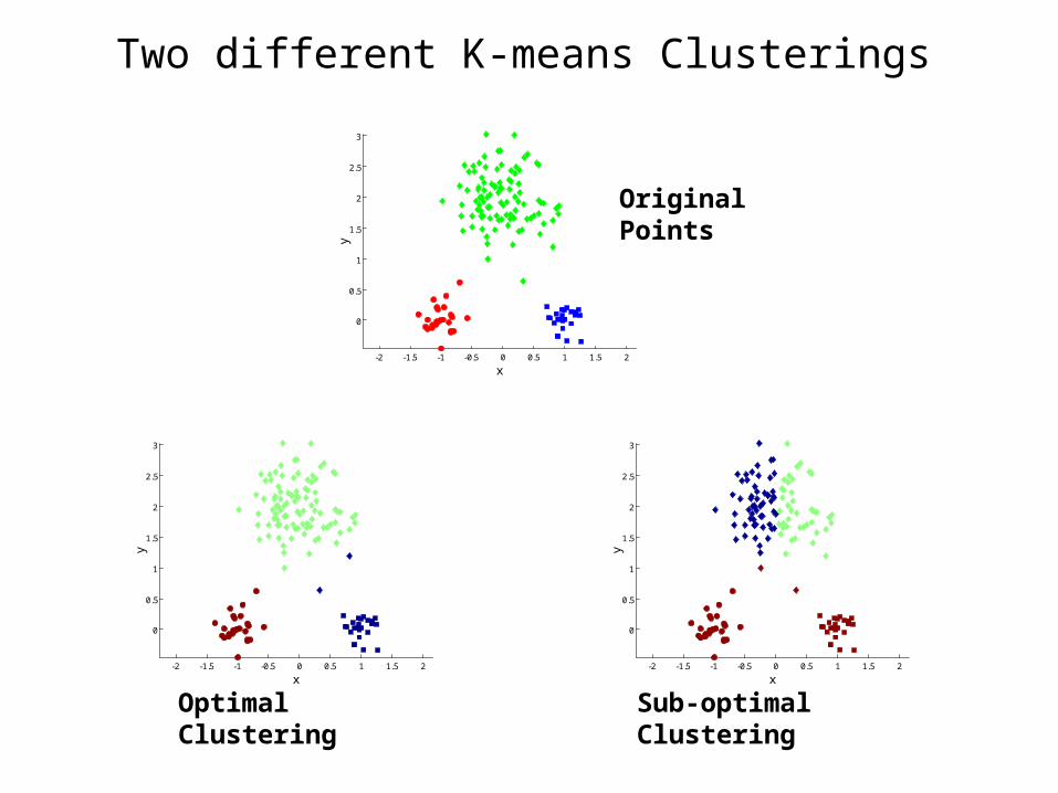
Two different K-means Clusterings
-2 -1.5 -1 -0.5 0 0.5 1 1.5 2
0
0.5
1
1.5
2
2.5
3
x
y
-2 -1.5 -1 -0.5 0 0.5 1 1.5 2
0
0.5
1
1.5
2
2.5
3
x
y
Sub-optimal Clustering
-2 -1.5 -1 -0.5 0 0.5 1 1.5 2
0
0.5
1
1.5
2
2.5
3
x
y
Optimal Clustering
Original Points
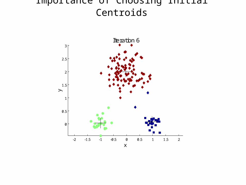
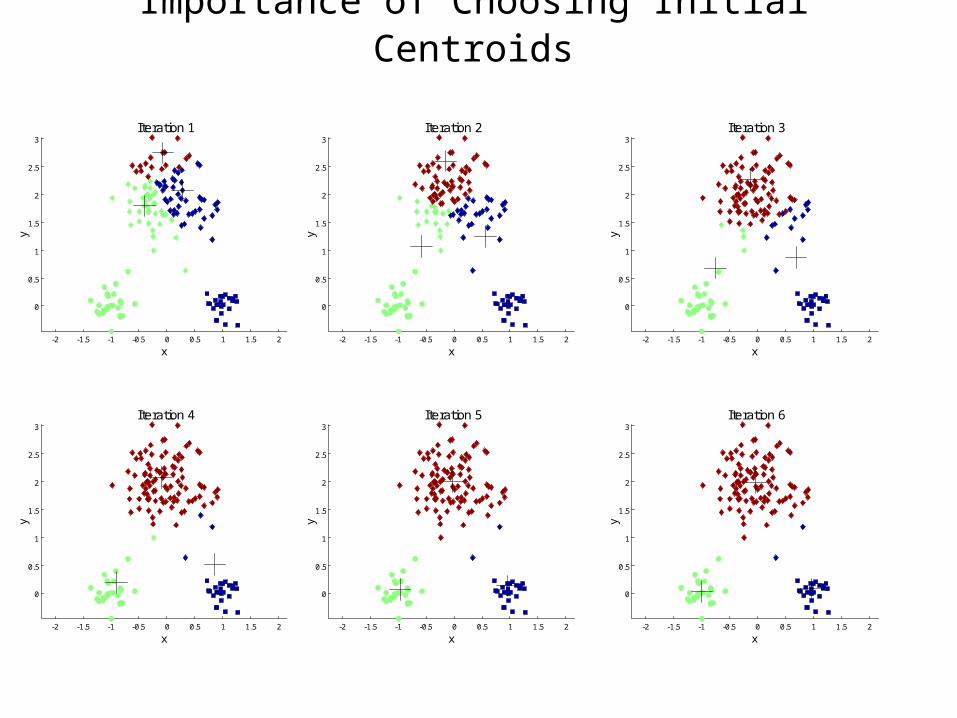
Importance of Choosing Initial Centroids
-2 -1.5 -1 -0.5 0 0.5 1 1.5 2
0
0.5
1
1.5
2
2.5
3
x
y
Iteration 1
-2 -1.5 -1 -0.5 0 0.5 1 1.5 2
0
0.5
1
1.5
2
2.5
3
x
y
Iteration 2
-2 -1.5 -1 -0.5 0 0.5 1 1.5 2
0
0.5
1
1.5
2
2.5
3
x
y
Iteration 3
-2 -1.5 -1 -0.5 0 0.5 1 1.5 2
0
0.5
1
1.5
2
2.5
3
x
y
Iteration 4
-2 -1.5 -1 -0.5 0 0.5 1 1.5 2
0
0.5
1
1.5
2
2.5
3
x
y
Iteration 5
-2 -1.5 -1 -0.5 0 0.5 1 1.5 2
0
0.5
1
1.5
2
2.5
3
x
y
Iteration 6
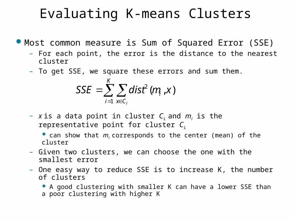
Evaluating K-means Clusters
Most common measure is Sum of Squared Error (SSE)– For each point, the error is the distance to the nearest cluster– To get SSE, we square these errors and sum them.
– x is a data point in cluster Ci and mi is the representative point for cluster Ci can show that mi corresponds to the center (mean) of the cluster
– Given two clusters, we can choose the one with the smallest error
– One easy way to reduce SSE is to increase K, the number of clusters A good clustering with smaller K can have a lower SSE than a poor clustering with higher K
K
i Cxi
i
xmdistSSE1
2 ),(
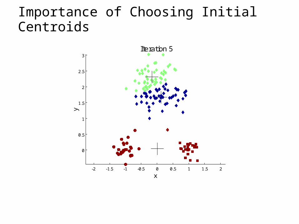
Importance of Choosing Initial Centroids
-2 -1.5 -1 -0.5 0 0.5 1 1.5 2
0
0.5
1
1.5
2
2.5
3
x
y
Iteration 1
-2 -1.5 -1 -0.5 0 0.5 1 1.5 2
0
0.5
1
1.5
2
2.5
3
x
y
Iteration 2
-2 -1.5 -1 -0.5 0 0.5 1 1.5 2
0
0.5
1
1.5
2
2.5
3
x
y
Iteration 3
-2 -1.5 -1 -0.5 0 0.5 1 1.5 2
0
0.5
1
1.5
2
2.5
3
x
y
Iteration 4
-2 -1.5 -1 -0.5 0 0.5 1 1.5 2
0
0.5
1
1.5
2
2.5
3
x
y
Iteration 5
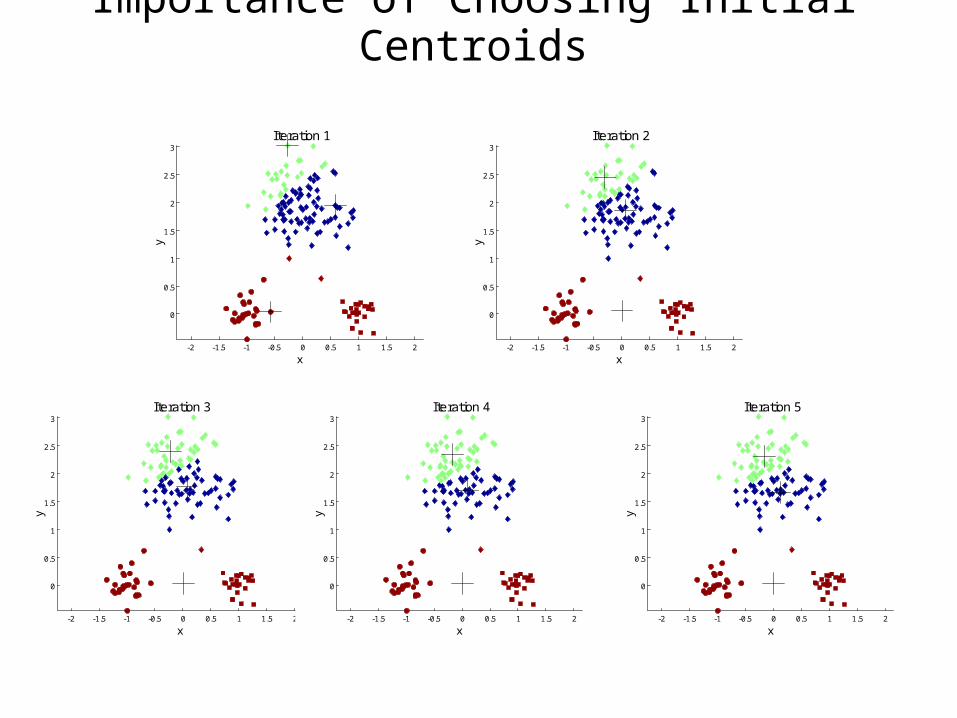
Importance of Choosing Initial Centroids
-2 -1.5 -1 -0.5 0 0.5 1 1.5 2
0
0.5
1
1.5
2
2.5
3
x
y
Iteration 1
-2 -1.5 -1 -0.5 0 0.5 1 1.5 2
0
0.5
1
1.5
2
2.5
3
x
y
Iteration 2
-2 -1.5 -1 -0.5 0 0.5 1 1.5 2
0
0.5
1
1.5
2
2.5
3
x
y
Iteration 3
-2 -1.5 -1 -0.5 0 0.5 1 1.5 2
0
0.5
1
1.5
2
2.5
3
x
y
Iteration 4
-2 -1.5 -1 -0.5 0 0.5 1 1.5 2
0
0.5
1
1.5
2
2.5
3
xy
Iteration 5
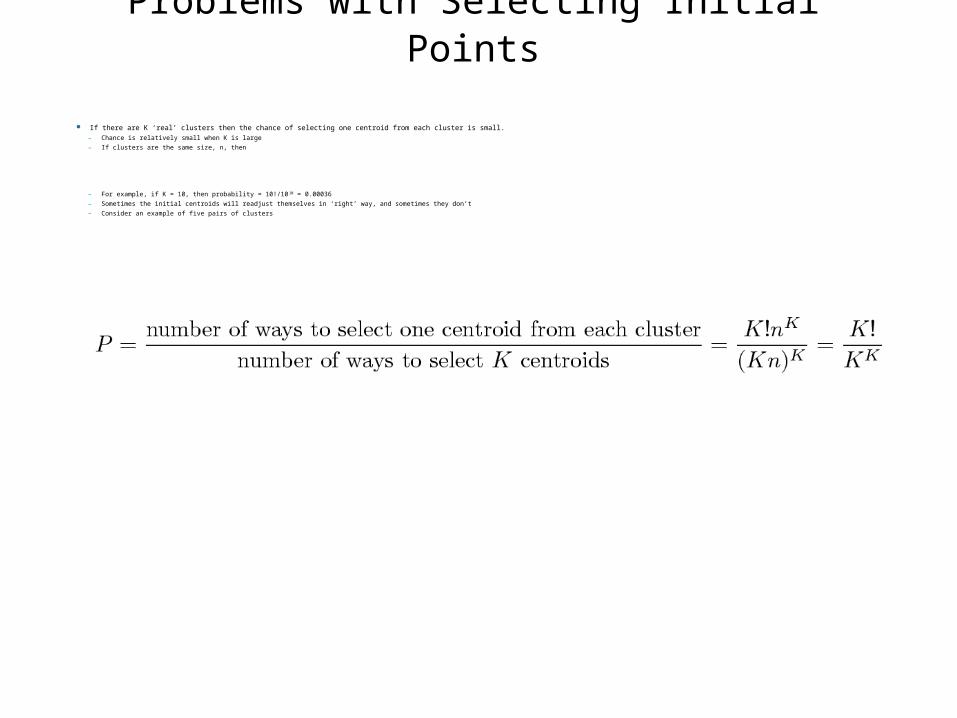
Problems with Selecting Initial Points
If there are K ‘real’ clusters then the chance of selecting one centroid from each cluster is small. – Chance is relatively small when K is large
– If clusters are the same size, n, then
– For example, if K = 10, then probability = 10!/1010 = 0.00036
– Sometimes the initial centroids will readjust themselves in ‘right’ way, and sometimes they don’t
– Consider an example of five pairs of clusters
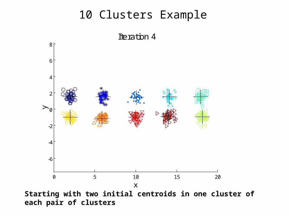
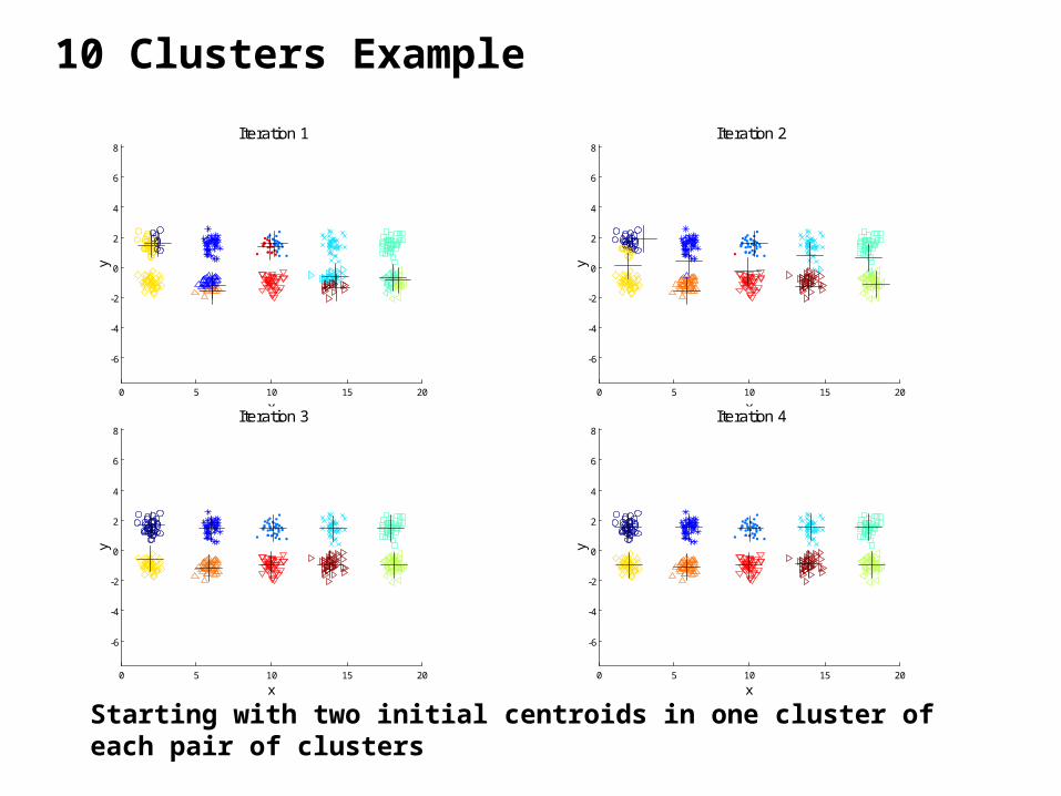
10 Clusters Example
0 5 10 15 20
-6
-4
-2
0
2
4
6
8
x
yIteration 1
0 5 10 15 20
-6
-4
-2
0
2
4
6
8
x
yIteration 2
0 5 10 15 20
-6
-4
-2
0
2
4
6
8
x
yIteration 3
0 5 10 15 20
-6
-4
-2
0
2
4
6
8
x
yIteration 4
Starting with two initial centroids in one cluster of each pair of clusters
10 Clusters Example
0 5 10 15 20
-6
-4
-2
0
2
4
6
8
x
y
Iteration 1
0 5 10 15 20
-6
-4
-2
0
2
4
6
8
x
y
Iteration 2
0 5 10 15 20
-6
-4
-2
0
2
4
6
8
x
y
Iteration 3
0 5 10 15 20
-6
-4
-2
0
2
4
6
8
x
y
Iteration 4
Starting with two initial centroids in one cluster of each pair of clusters
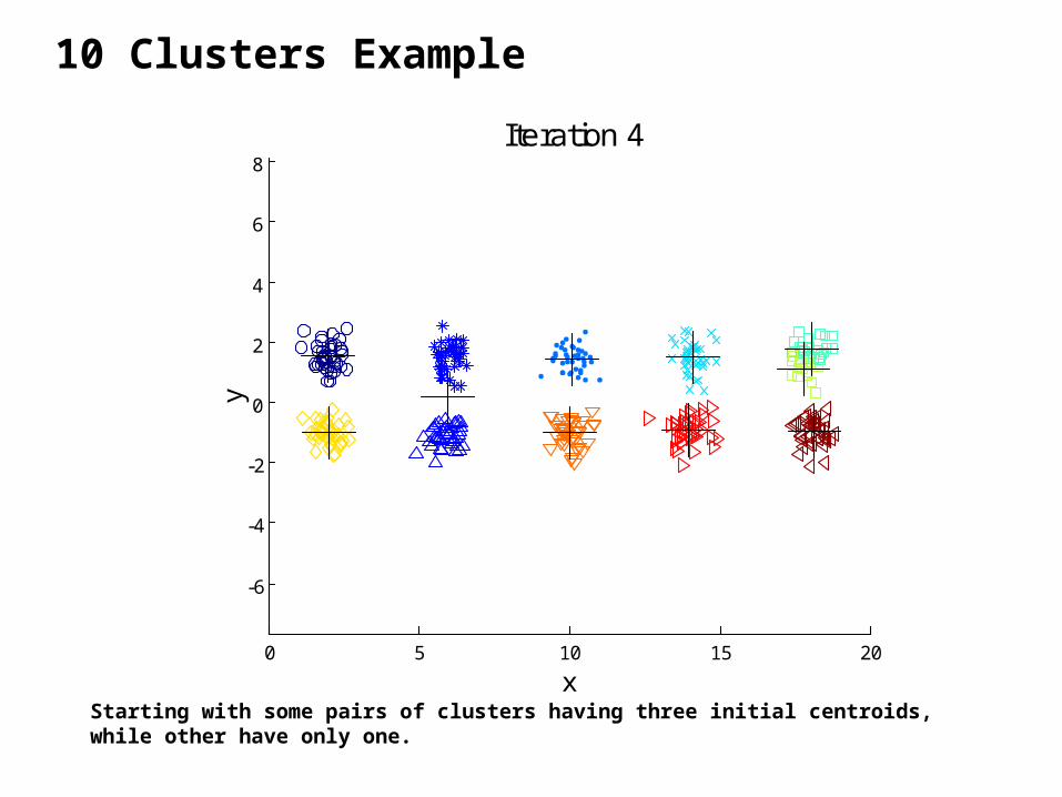
10 Clusters Example
Starting with some pairs of clusters having three initial centroids, while other have only one.
0 5 10 15 20
-6
-4
-2
0
2
4
6
8
x
y
Iteration 1
0 5 10 15 20
-6
-4
-2
0
2
4
6
8
x
y
Iteration 2
0 5 10 15 20
-6
-4
-2
0
2
4
6
8
x
y
Iteration 3
0 5 10 15 20
-6
-4
-2
0
2
4
6
8
x
y
Iteration 4
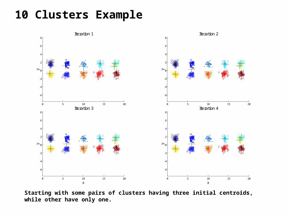
10 Clusters Example
Starting with some pairs of clusters having three initial centroids, while other have only one.
0 5 10 15 20
-6
-4
-2
0
2
4
6
8
x
yIteration 1
0 5 10 15 20
-6
-4
-2
0
2
4
6
8
x
y
Iteration 2
0 5 10 15 20
-6
-4
-2
0
2
4
6
8
x
y
Iteration 3
0 5 10 15 20
-6
-4
-2
0
2
4
6
8
x
y
Iteration 4
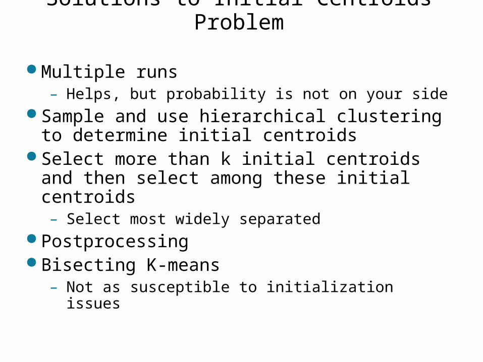
Solutions to Initial Centroids Problem
Multiple runs– Helps, but probability is not on your side
Sample and use hierarchical clustering to determine initial centroids
Select more than k initial centroids and then select among these initial centroids– Select most widely separated
Postprocessing Bisecting K-means
– Not as susceptible to initialization issues
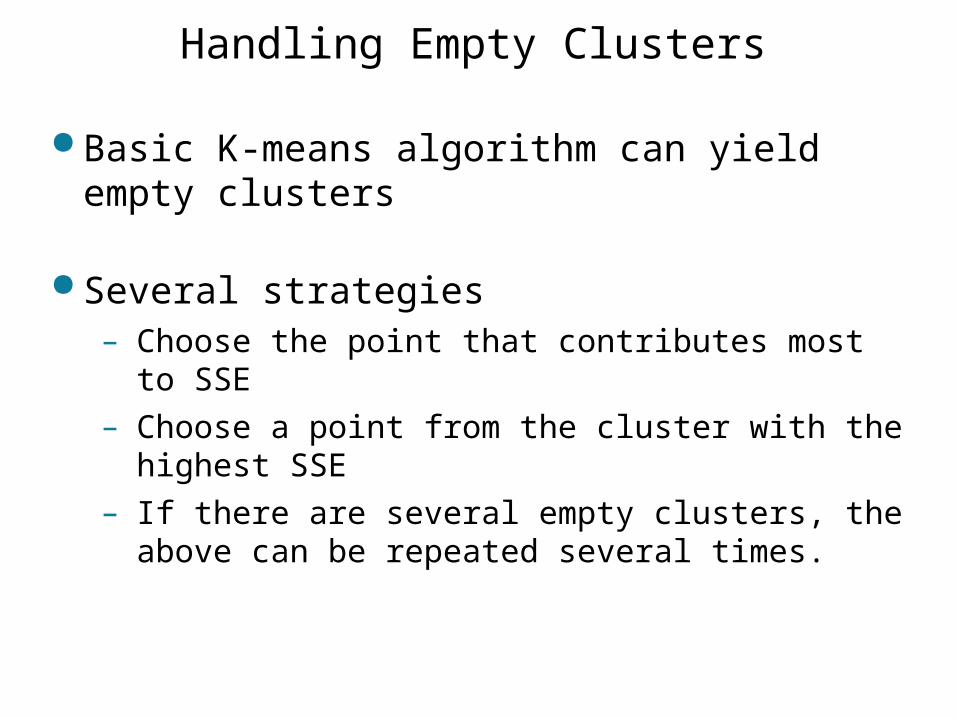
Handling Empty Clusters
Basic K-means algorithm can yield empty clusters
Several strategies– Choose the point that contributes most to SSE– Choose a point from the cluster with the
highest SSE– If there are several empty clusters, the above
can be repeated several times.
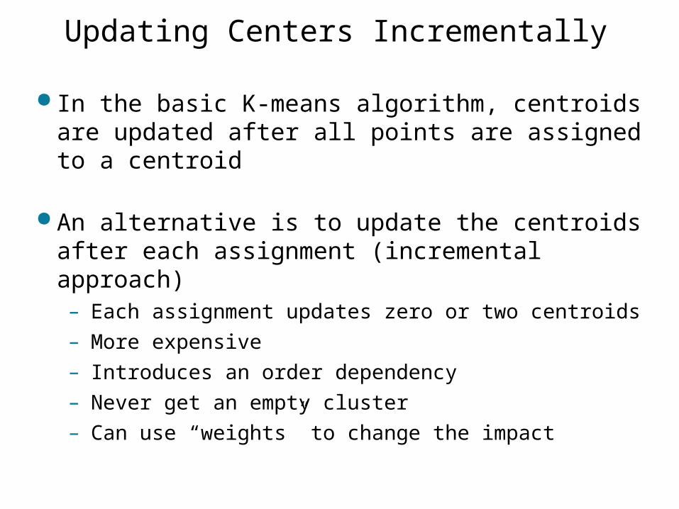
Updating Centers Incrementally
In the basic K-means algorithm, centroids are updated after all points are assigned to a centroid
An alternative is to update the centroids after each assignment (incremental approach)– Each assignment updates zero or two centroids– More expensive– Introduces an order dependency– Never get an empty cluster– Can use “weights” to change the impact
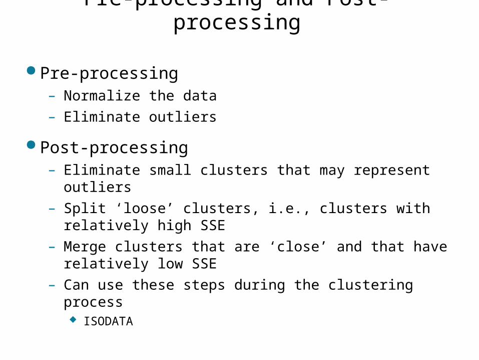
Pre-processing and Post-processing
Pre-processing– Normalize the data– Eliminate outliers
Post-processing– Eliminate small clusters that may represent
outliers– Split ‘loose’ clusters, i.e., clusters with relatively
high SSE– Merge clusters that are ‘close’ and that have
relatively low SSE– Can use these steps during the clustering process
ISODATA
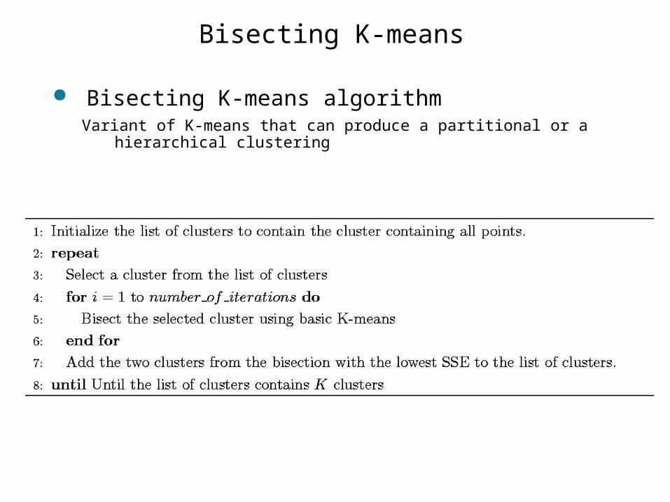
Bisecting K-means
Bisecting K-means algorithmVariant of K-means that can produce a partitional or a hierarchical
clustering
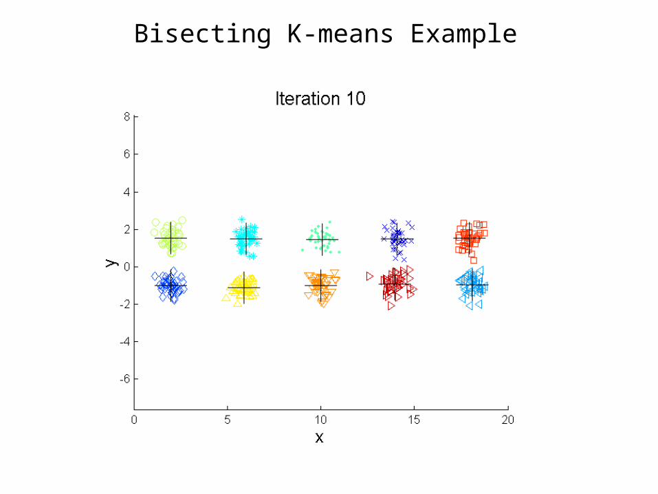
Bisecting K-means Example
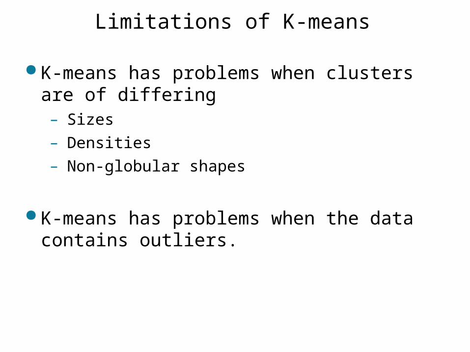
Limitations of K-means
K-means has problems when clusters are of differing – Sizes– Densities– Non-globular shapes
K-means has problems when the data contains outliers.
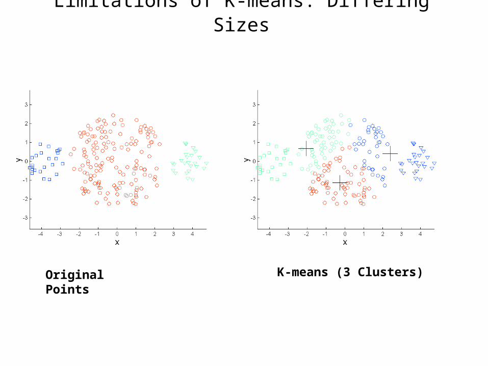
Limitations of K-means: Differing Sizes
Original Points
K-means (3 Clusters)
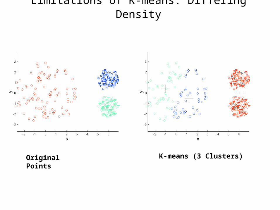
Limitations of K-means: Differing Density
Original Points K-means (3 Clusters)
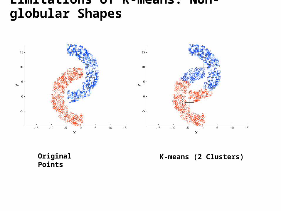
Limitations of K-means: Non-globular Shapes
Original Points
K-means (2 Clusters)
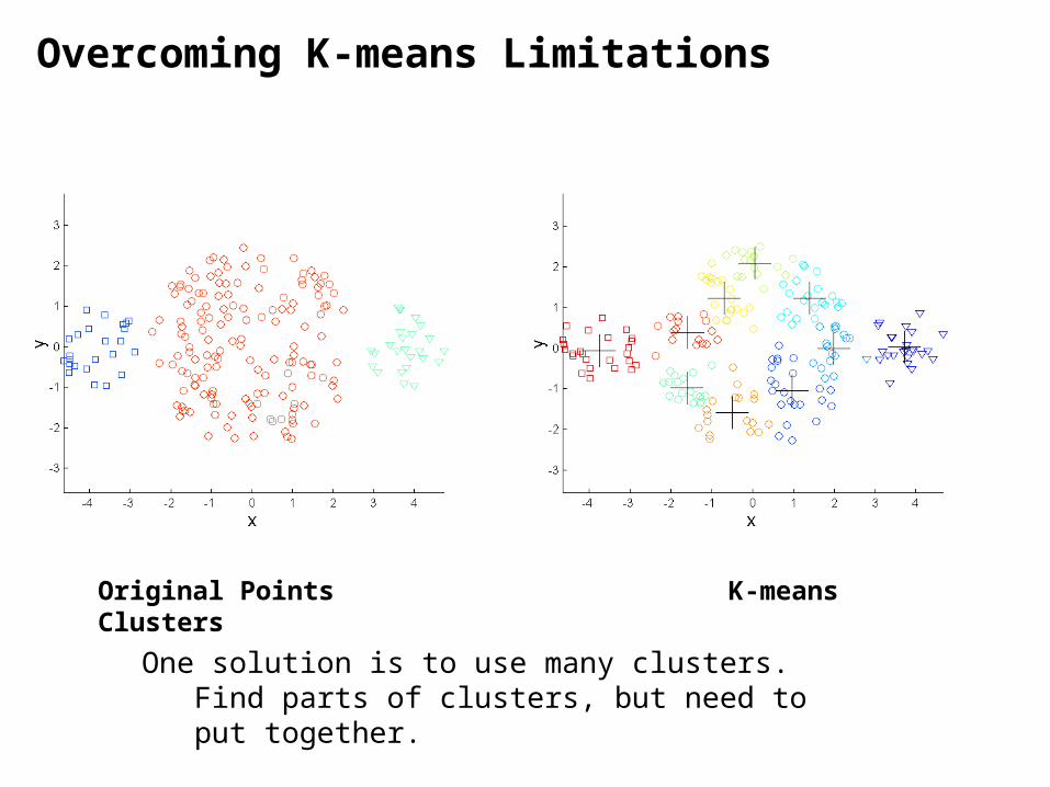
Overcoming K-means Limitations
Original Points K-means Clusters
One solution is to use many clusters.Find parts of clusters, but need to put together.
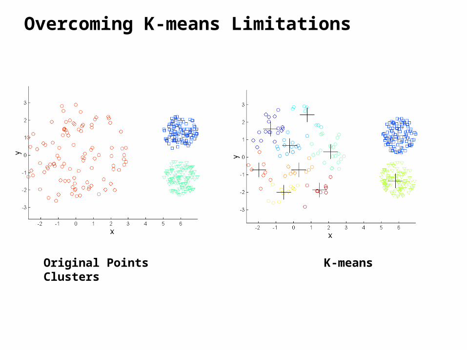
Overcoming K-means Limitations
Original Points K-means Clusters
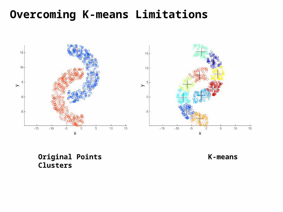
Overcoming K-means Limitations
Original Points K-means Clusters
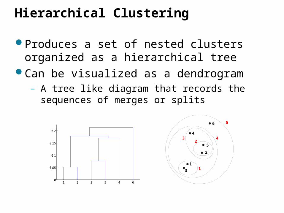
Hierarchical Clustering
Produces a set of nested clusters organized as a hierarchical tree
Can be visualized as a dendrogram– A tree like diagram that records the sequences
of merges or splits
1 3 2 5 4 60
0.05
0.1
0.15
0.2
1
2
3
4
5
6
1
23 4
5
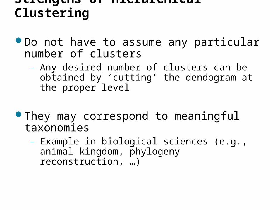
Strengths of Hierarchical Clustering
Do not have to assume any particular number of clusters– Any desired number of clusters can be
obtained by ‘cutting’ the dendogram at the proper level
They may correspond to meaningful taxonomies– Example in biological sciences (e.g., animal
kingdom, phylogeny reconstruction, …)
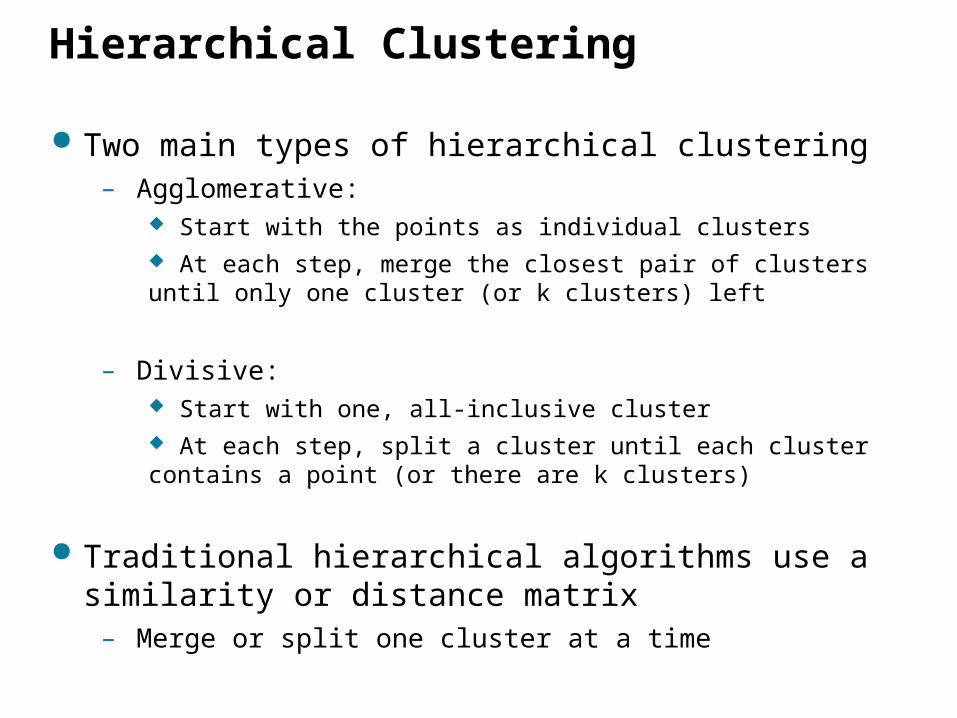
Hierarchical Clustering
Two main types of hierarchical clustering– Agglomerative:
Start with the points as individual clusters At each step, merge the closest pair of clusters until only one cluster (or k clusters) left
– Divisive: Start with one, all-inclusive cluster At each step, split a cluster until each cluster contains a point (or there are k clusters)
Traditional hierarchical algorithms use a similarity or distance matrix
– Merge or split one cluster at a time
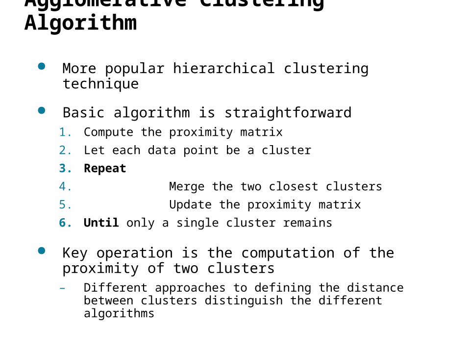
Agglomerative Clustering Algorithm
More popular hierarchical clustering technique
Basic algorithm is straightforward1. Compute the proximity matrix
2. Let each data point be a cluster
3. Repeat
4. Merge the two closest clusters
5. Update the proximity matrix
6. Until only a single cluster remains
Key operation is the computation of the proximity of two clusters– Different approaches to defining the distance
between clusters distinguish the different algorithms
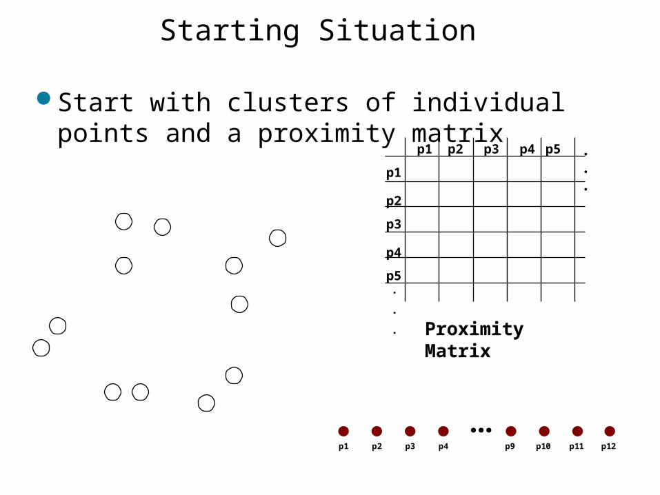
Starting Situation
Start with clusters of individual points and a proximity matrix
p1
p3
p5
p4
p2
p1 p2 p3 p4 p5 . . .
.
.
. Proximity Matrix
...p1 p2 p3 p4 p9 p10 p11 p12
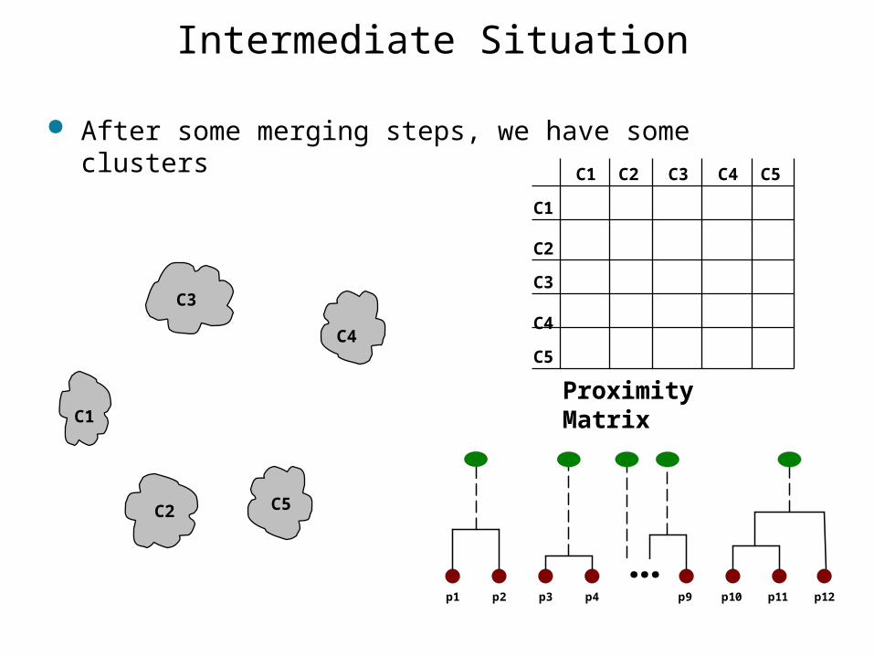
Intermediate Situation
After some merging steps, we have some clusters
C1
C4
C2 C5
C3
C2C1
C1
C3
C5
C4
C2
C3 C4 C5
Proximity Matrix
...p1 p2 p3 p4 p9 p10 p11 p12
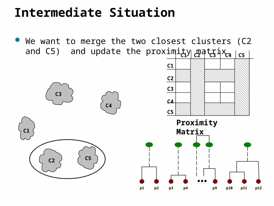
Intermediate Situation
We want to merge the two closest clusters (C2 and C5) and update the proximity matrix.
C1
C4
C2 C5
C3
C2C1
C1
C3
C5
C4
C2
C3 C4 C5
Proximity Matrix
...p1 p2 p3 p4 p9 p10 p11 p12
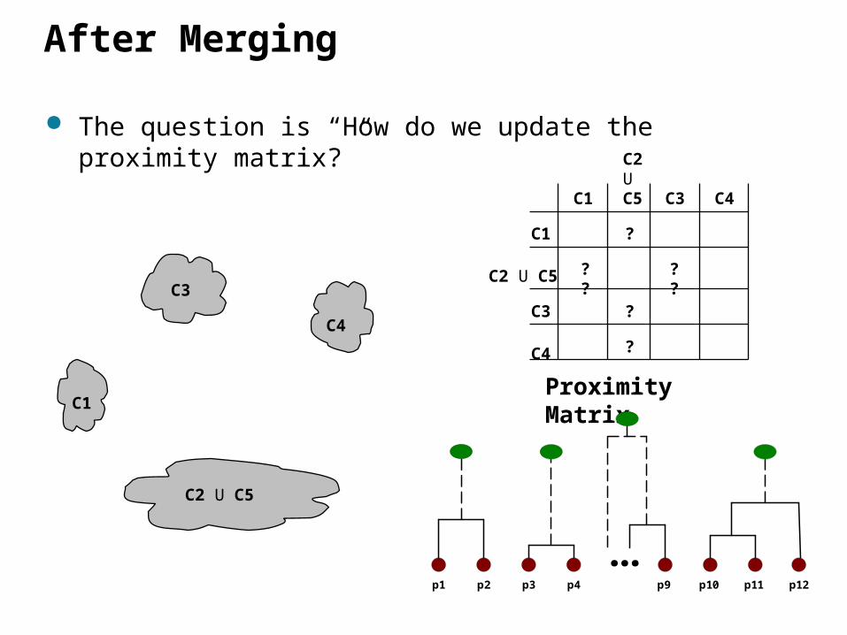
After Merging
The question is “How do we update the proximity matrix?”
C1
C4
C2 U C5
C3? ? ? ?
?
?
?
C2 U C5C1
C1
C3
C4
C2 U C5
C3 C4
Proximity Matrix
...p1 p2 p3 p4 p9 p10 p11 p12
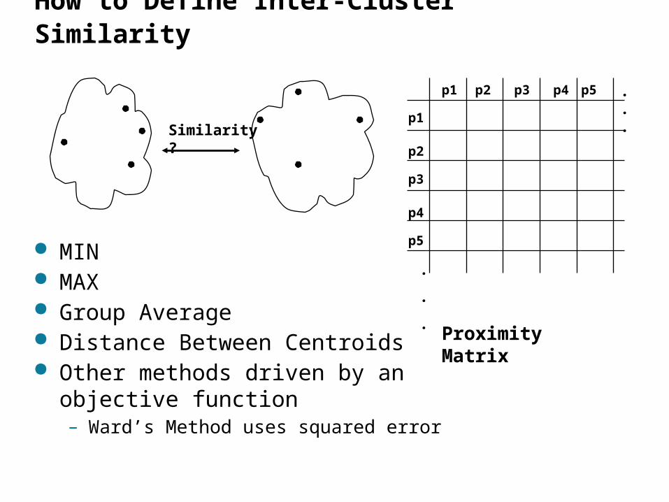
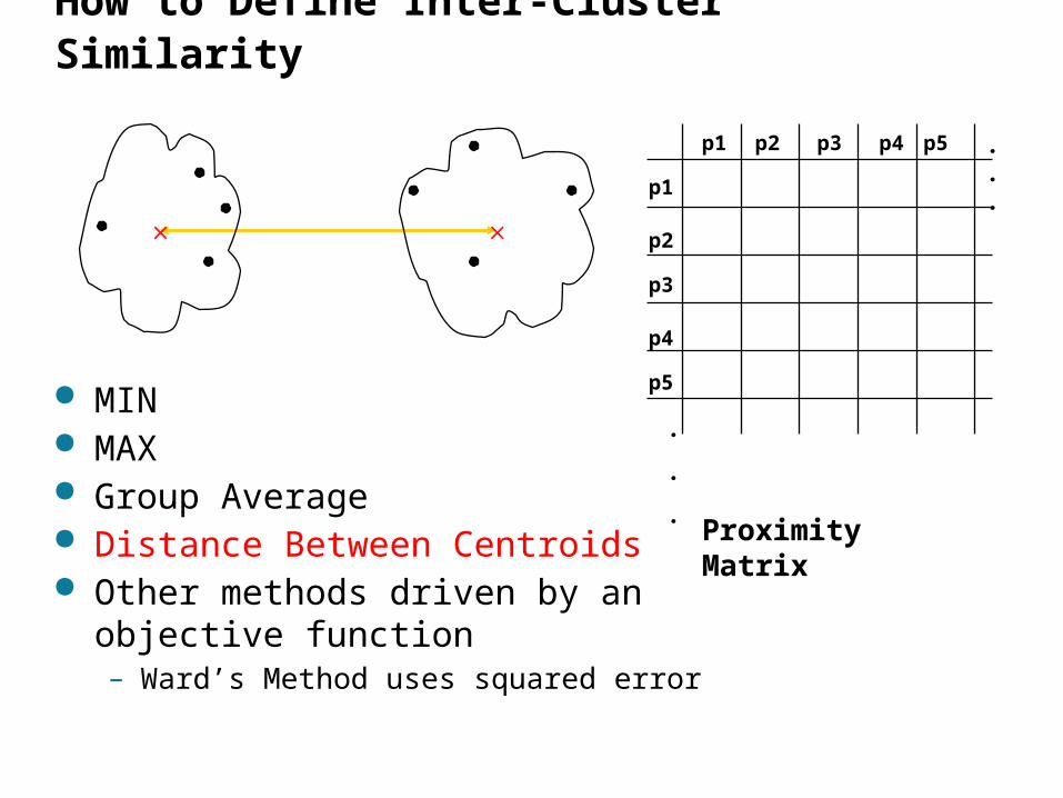
How to Define Inter-Cluster Similarity
p1
p3
p5
p4
p2
p1 p2 p3 p4 p5 . . .
.
.
.
Similarity?
MIN MAX Group Average Distance Between Centroids Other methods driven by an
objective function– Ward’s Method uses squared error
Proximity Matrix
How to Define Inter-Cluster Similarity
p1
p3
p5
p4
p2
p1 p2 p3 p4 p5 . . .
.
.
.Proximity Matrix
MIN MAX Group Average Distance Between Centroids Other methods driven by an
objective function– Ward’s Method uses squared error
How to Define Inter-Cluster Similarity
p1
p3
p5
p4
p2
p1 p2 p3 p4 p5 . . .
.
.
.Proximity Matrix
MIN MAX Group Average Distance Between Centroids Other methods driven by an
objective function– Ward’s Method uses squared error
How to Define Inter-Cluster Similarity
p1
p3
p5
p4
p2
p1 p2 p3 p4 p5 . . .
.
.
.Proximity Matrix
MIN MAX Group Average Distance Between Centroids Other methods driven by an
objective function– Ward’s Method uses squared error
How to Define Inter-Cluster Similarity
p1
p3
p5
p4
p2
p1 p2 p3 p4 p5 . . .
.
.
.Proximity Matrix
MIN MAX Group Average Distance Between Centroids Other methods driven by an
objective function– Ward’s Method uses squared error
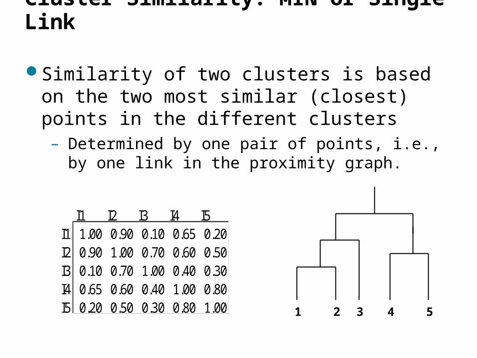
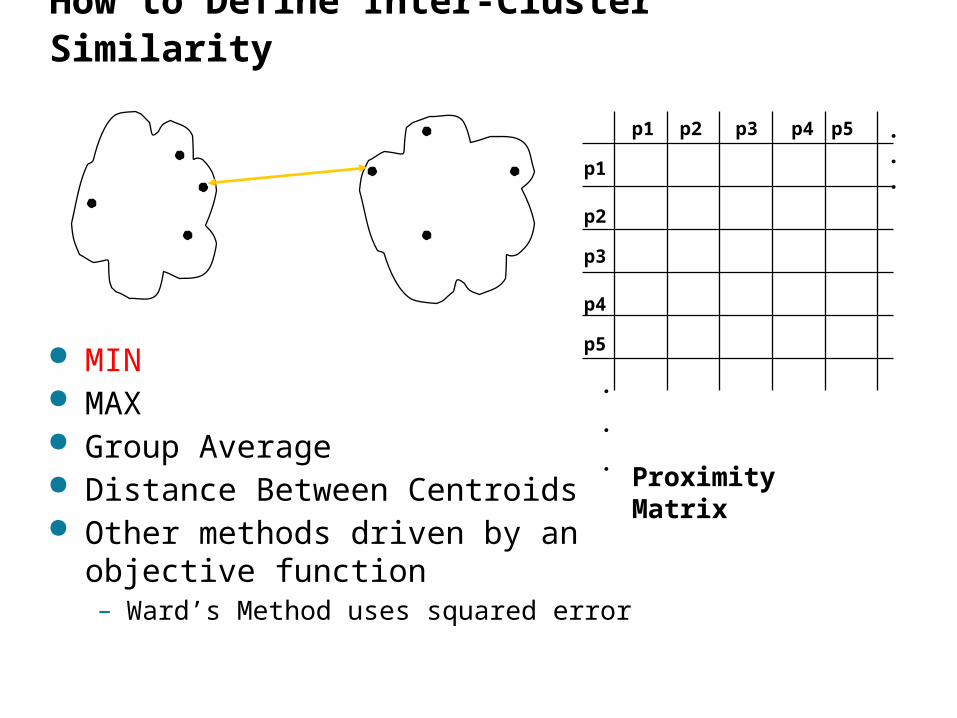
Cluster Similarity: MIN or Single Link
Similarity of two clusters is based on the two most similar (closest) points in the different clusters– Determined by one pair of points, i.e., by one
link in the proximity graph.
I1 I2 I3 I4 I5I1 1.00 0.90 0.10 0.65 0.20I2 0.90 1.00 0.70 0.60 0.50I3 0.10 0.70 1.00 0.40 0.30I4 0.65 0.60 0.40 1.00 0.80I5 0.20 0.50 0.30 0.80 1.00 1 2 3 4 5
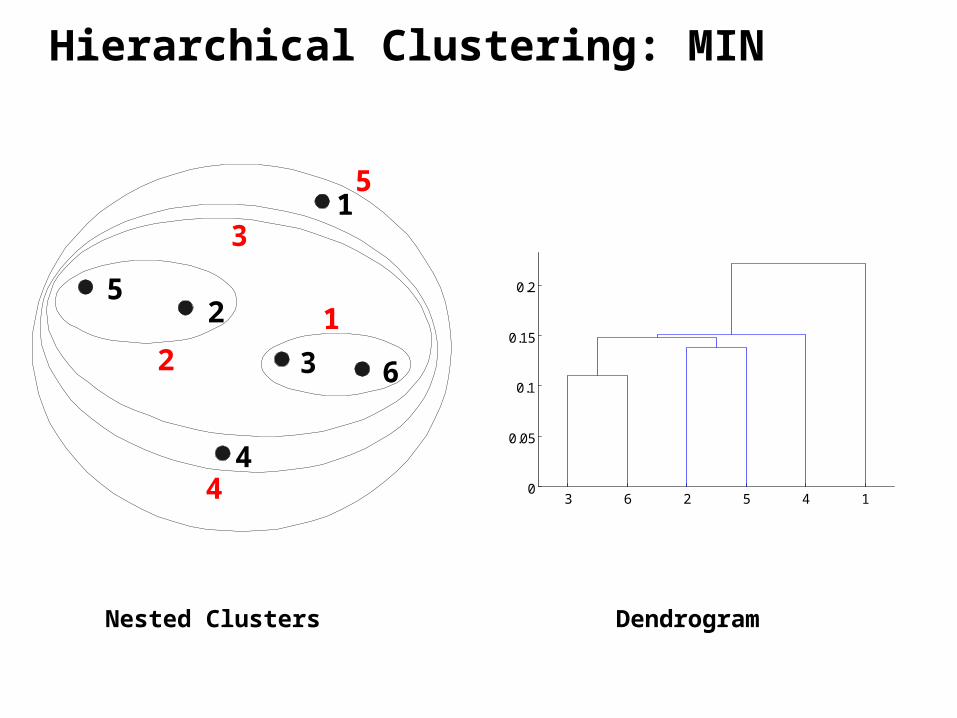
Hierarchical Clustering: MIN
Nested Clusters Dendrogram
1
2
3
4
5
6
12
3
4
5
3 6 2 5 4 10
0.05
0.1
0.15
0.2
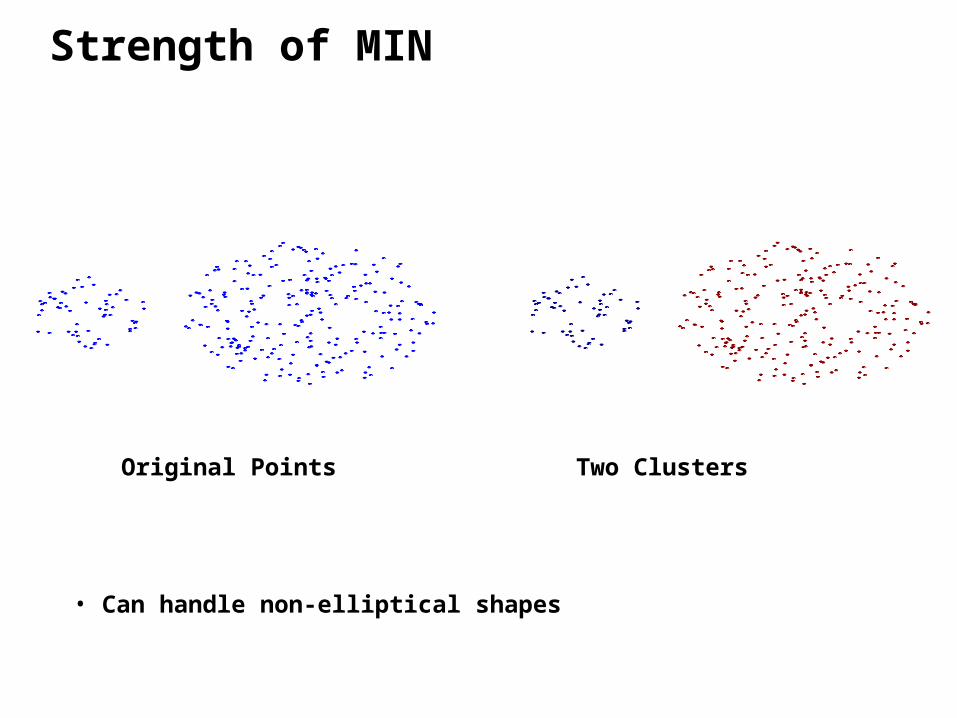
Strength of MIN
Original Points Two Clusters
• Can handle non-elliptical shapes
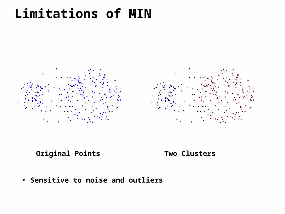
Limitations of MIN
Original Points Two Clusters
• Sensitive to noise and outliers
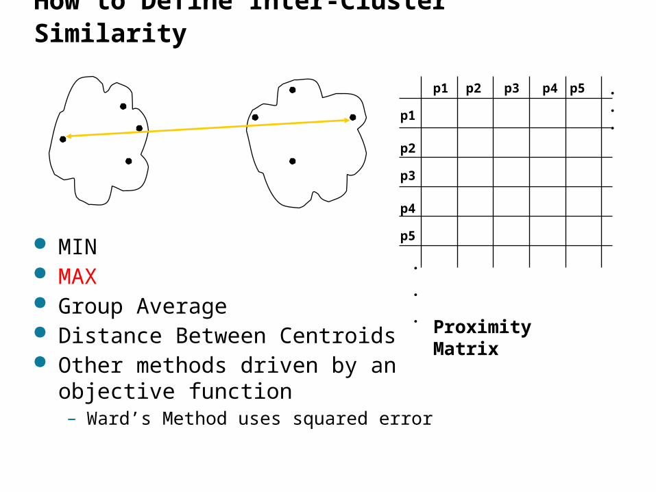
Cluster Similarity: MAX or Complete Linkage
Similarity of two clusters is based on the two least similar (most distant) points in the different clusters– Determined by all pairs of points in the two
clusters
I1 I2 I3 I4 I5I1 1.00 0.90 0.10 0.65 0.20I2 0.90 1.00 0.70 0.60 0.50I3 0.10 0.70 1.00 0.40 0.30I4 0.65 0.60 0.40 1.00 0.80I5 0.20 0.50 0.30 0.80 1.00 1 2 3 4 5
Hierarchical Clustering: MAX
Nested Clusters Dendrogram
3 6 4 1 2 50
0.05
0.1
0.15
0.2
0.25
0.3
0.35
0.4
1
2
3
4
5
6
1
2 5
3
4
Strength of MAX
Original Points Two Clusters
• Less susceptible to noise and outliers
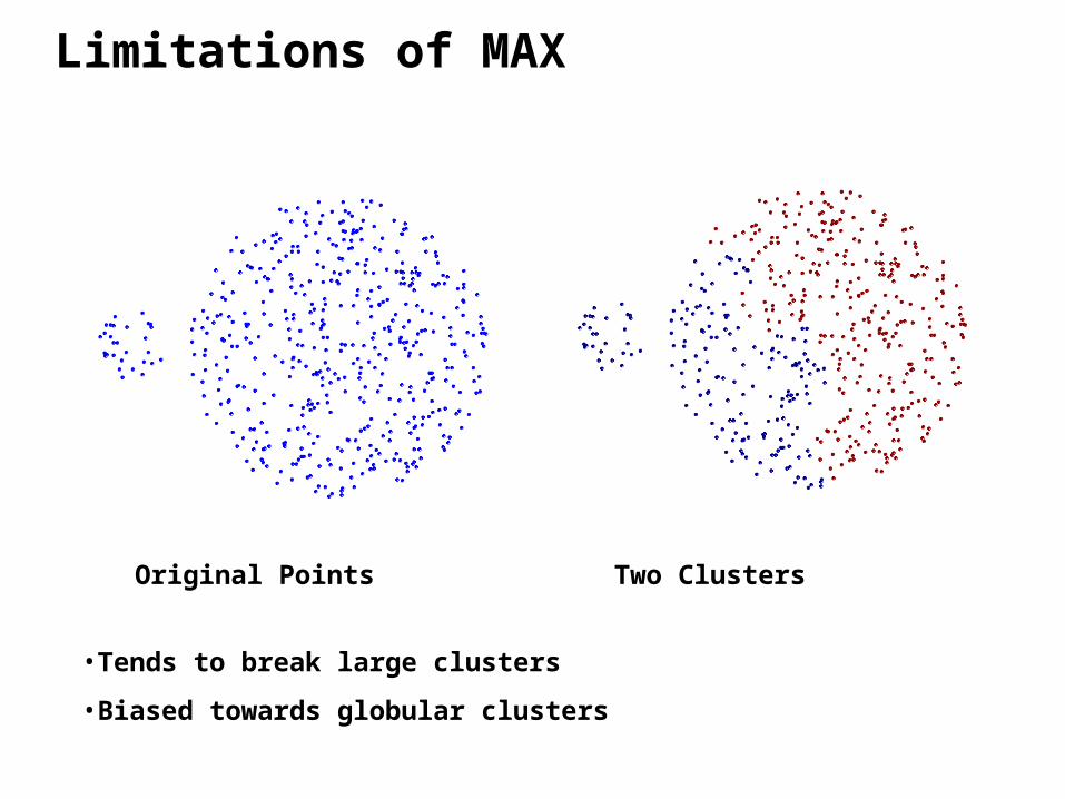
Limitations of MAX
Original Points Two Clusters
•Tends to break large clusters
•Biased towards globular clusters
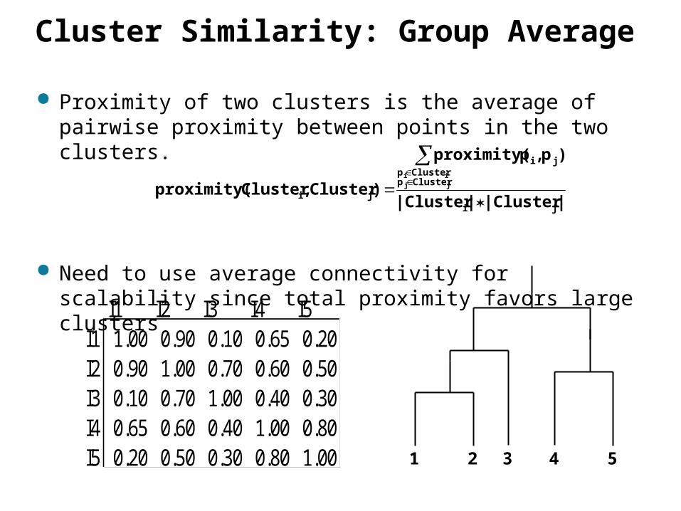
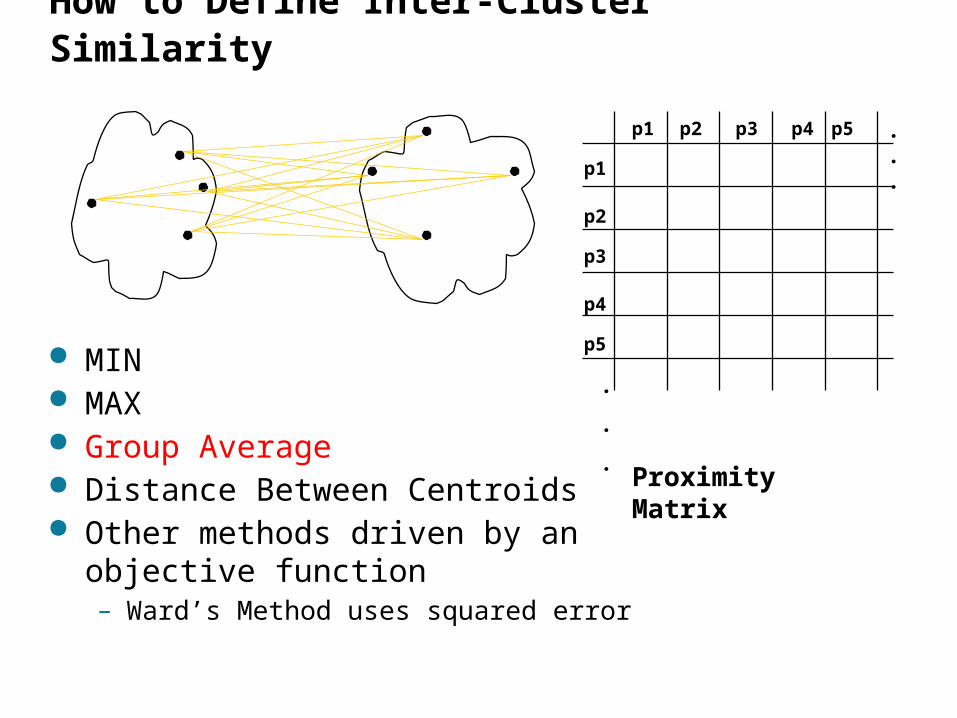
Cluster Similarity: Group Average
Proximity of two clusters is the average of pairwise proximity between points in the two clusters.
Need to use average connectivity for scalability since total proximity favors large clusters
||Cluster||Cluster
)p,pproximity(
)Cluster,Clusterproximity(ji
ClusterpClusterp
ji
jijjii
I1 I2 I3 I4 I5I1 1.00 0.90 0.10 0.65 0.20I2 0.90 1.00 0.70 0.60 0.50I3 0.10 0.70 1.00 0.40 0.30I4 0.65 0.60 0.40 1.00 0.80I5 0.20 0.50 0.30 0.80 1.00 1 2 3 4 5
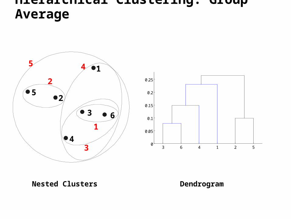
Hierarchical Clustering: Group Average
Nested Clusters Dendrogram
3 6 4 1 2 50
0.05
0.1
0.15
0.2
0.25
1
2
3
4
5
6
1
2
5
3
4
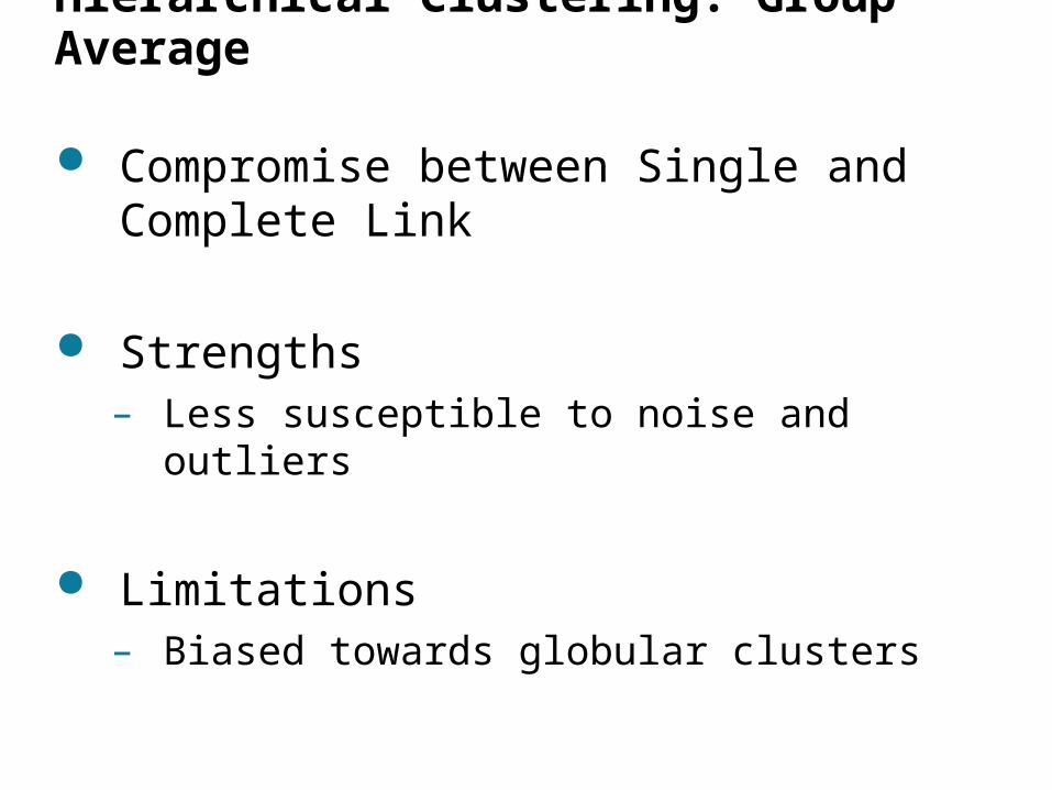
Hierarchical Clustering: Group Average
Compromise between Single and Complete Link
Strengths– Less susceptible to noise and outliers
Limitations– Biased towards globular clusters
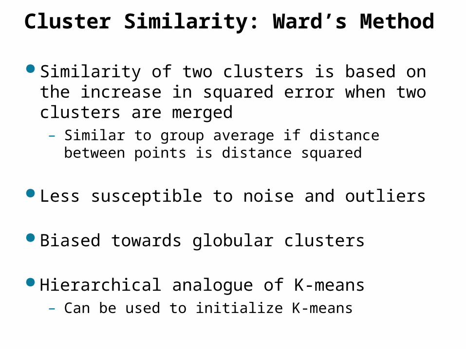
Cluster Similarity: Ward’s Method
Similarity of two clusters is based on the increase in squared error when two clusters are merged– Similar to group average if distance between
points is distance squared
Less susceptible to noise and outliers
Biased towards globular clusters
Hierarchical analogue of K-means– Can be used to initialize K-means
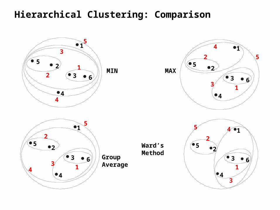
Hierarchical Clustering: Comparison
Group Average
Ward’s Method
1
2
3
4
5
61
2
5
3
4
MIN MAX
1
2
3
4
5
61
2
5
34
1
2
3
4
5
61
2 5
3
41
2
3
4
5
6
12
3
4
5
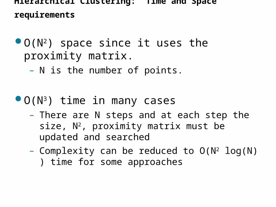
Hierarchical Clustering: Time and Space
requirements
O(N2) space since it uses the proximity matrix. – N is the number of points.
O(N3) time in many cases– There are N steps and at each step the size, N2,
proximity matrix must be updated and searched
– Complexity can be reduced to O(N2 log(N) ) time for some approaches
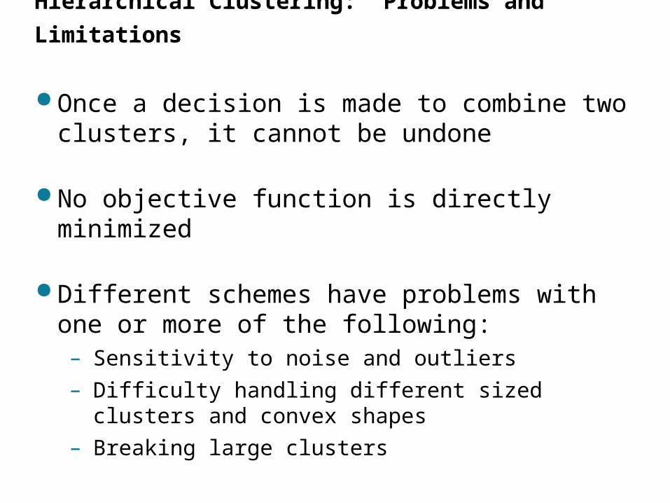
Hierarchical Clustering: Problems and
Limitations
Once a decision is made to combine two clusters, it cannot be undone
No objective function is directly minimized
Different schemes have problems with one or more of the following:– Sensitivity to noise and outliers– Difficulty handling different sized clusters and
convex shapes– Breaking large clusters
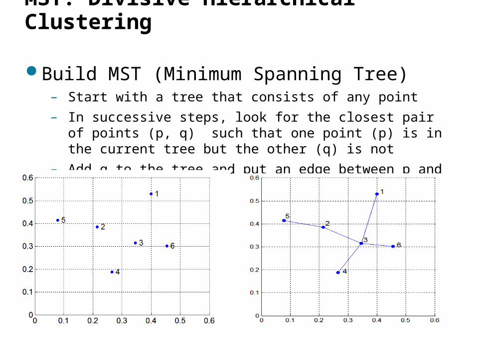
MST: Divisive Hierarchical Clustering
Build MST (Minimum Spanning Tree)– Start with a tree that consists of any point
– In successive steps, look for the closest pair of points (p, q) such that one point (p) is in the current tree but the other (q) is not
– Add q to the tree and put an edge between p and q
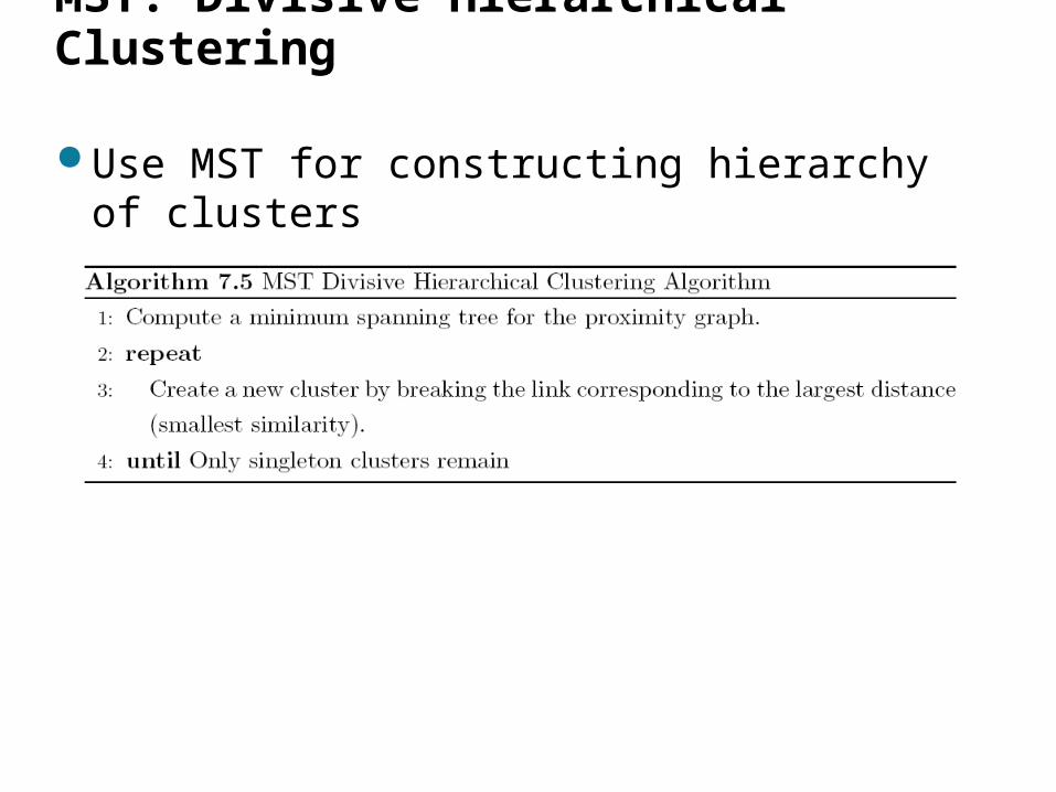
MST: Divisive Hierarchical Clustering
Use MST for constructing hierarchy of clusters
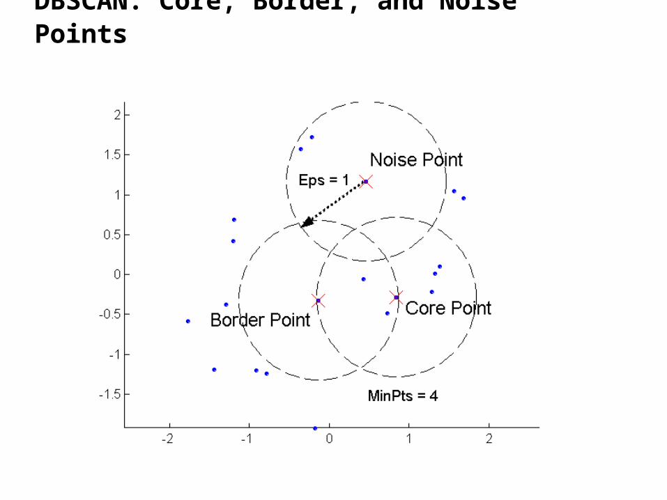
DBSCAN
DBSCAN is a density-based algorithm.– Density = number of points within a specified radius
(Eps)
– A point is a core point if it has more than a specified number of points (MinPts) within Eps
These are points that are at the interior of a cluster
– A border point has fewer than MinPts within Eps, but is in the neighborhood of a core point
– A noise point is any point that is not a core point or a border point.
DBSCAN: Core, Border, and Noise Points
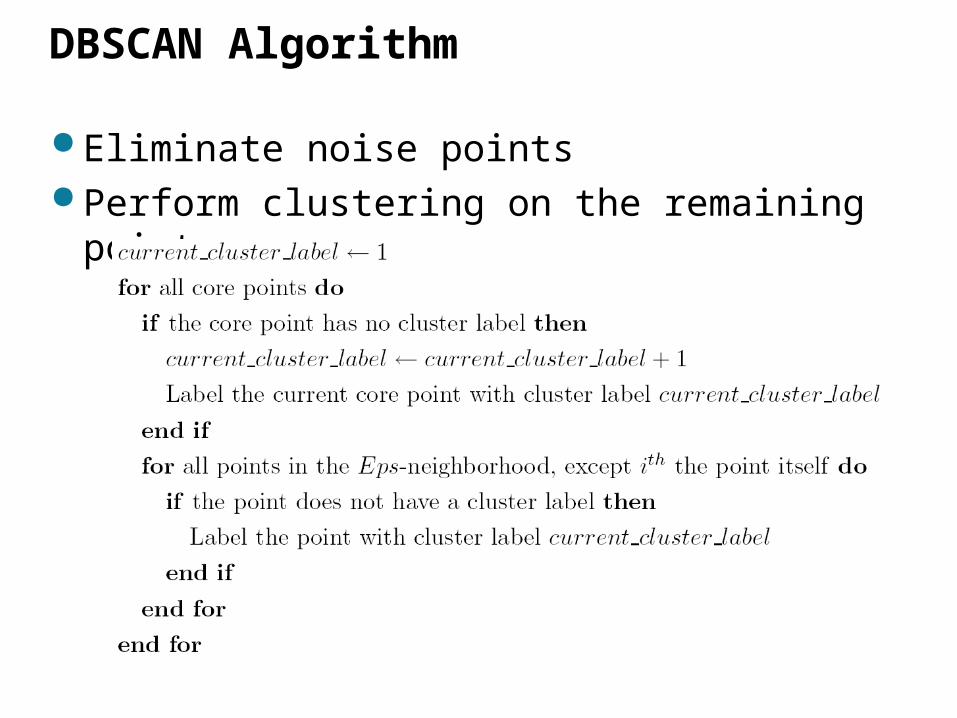
DBSCAN Algorithm
Eliminate noise points Perform clustering on the remaining points
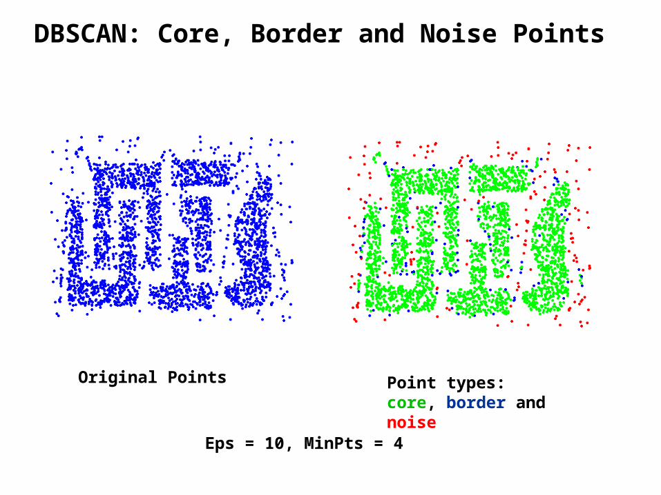
DBSCAN: Core, Border and Noise Points
Original Points Point types: core, border and noise
Eps = 10, MinPts = 4
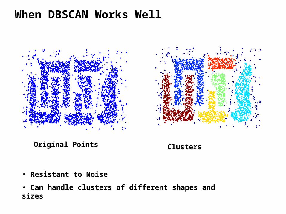
When DBSCAN Works Well
Original Points Clusters
• Resistant to Noise
• Can handle clusters of different shapes and sizes
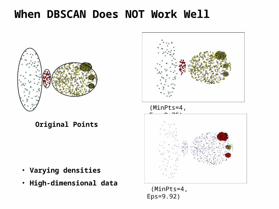
When DBSCAN Does NOT Work Well
Original Points
(MinPts=4, Eps=9.75).
(MinPts=4, Eps=9.92)
• Varying densities
• High-dimensional data
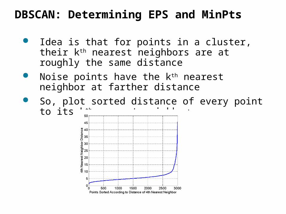
DBSCAN: Determining EPS and MinPts
Idea is that for points in a cluster, their kth nearest neighbors are at roughly the same distance
Noise points have the kth nearest neighbor at farther distance
So, plot sorted distance of every point to its kth nearest neighbor
Cluster Validity
For supervised classification we have a variety of measures to evaluate how good our model is
– Accuracy, precision, recall
For cluster analysis, the analogous question is how to evaluate the “goodness” of the resulting clusters?
But “clusters are in the eye of the beholder”!
Then why do we want to evaluate them?– To avoid finding patterns in noise– To compare clustering algorithms– To compare two sets of clusters– To compare two clusters
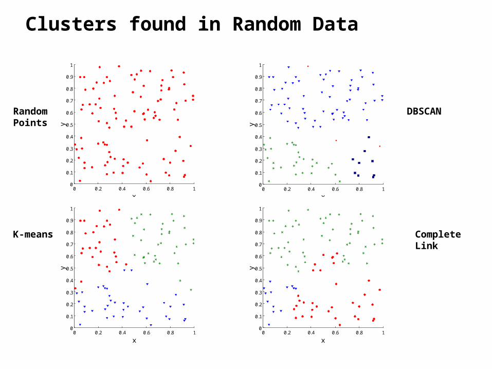
Clusters found in Random Data
0 0.2 0.4 0.6 0.8 10
0.1
0.2
0.3
0.4
0.5
0.6
0.7
0.8
0.9
1
x
y
Random Points
0 0.2 0.4 0.6 0.8 10
0.1
0.2
0.3
0.4
0.5
0.6
0.7
0.8
0.9
1
x
y
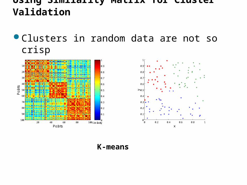
K-means
0 0.2 0.4 0.6 0.8 10
0.1
0.2
0.3
0.4
0.5
0.6
0.7
0.8
0.9
1
x
y
DBSCAN
0 0.2 0.4 0.6 0.8 10
0.1
0.2
0.3
0.4
0.5
0.6
0.7
0.8
0.9
1
x
y
Complete Link
1. Determining the clustering tendency of a set of data, i.e., distinguishing whether non-random structure actually exists in the data.
2. Comparing the results of a cluster analysis to externally known results, e.g., to externally given class labels.
3. Evaluating how well the results of a cluster analysis fit the data without reference to external information.
- Use only the data
4. Comparing the results of two different sets of cluster analyses to determine which is better.
5. Determining the ‘correct’ number of clusters.
For 2, 3, and 4, we can further distinguish whether we want to evaluate the entire clustering or just individual clusters.
Different Aspects of Cluster Validation
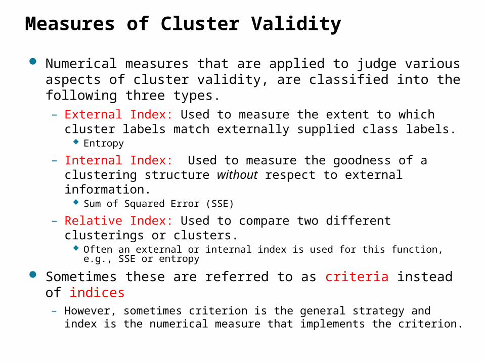
Numerical measures that are applied to judge various aspects of cluster validity, are classified into the following three types.– External Index: Used to measure the extent to which cluster
labels match externally supplied class labels. Entropy
– Internal Index: Used to measure the goodness of a clustering structure without respect to external information.
Sum of Squared Error (SSE)
– Relative Index: Used to compare two different clusterings or clusters.
Often an external or internal index is used for this function, e.g., SSE or entropy
Sometimes these are referred to as criteria instead of indices– However, sometimes criterion is the general strategy and index is
the numerical measure that implements the criterion.
Measures of Cluster Validity
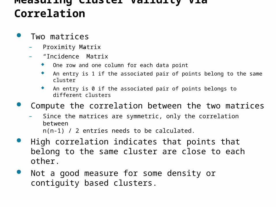
Two matrices – Proximity Matrix
– “Incidence” Matrix One row and one column for each data point An entry is 1 if the associated pair of points belong to the same cluster An entry is 0 if the associated pair of points belongs to different clusters
Compute the correlation between the two matrices– Since the matrices are symmetric, only the correlation between
n(n-1) / 2 entries needs to be calculated.
High correlation indicates that points that belong to the same cluster are close to each other.
Not a good measure for some density or contiguity based clusters.
Measuring Cluster Validity Via Correlation
Measuring Cluster Validity Via Correlation
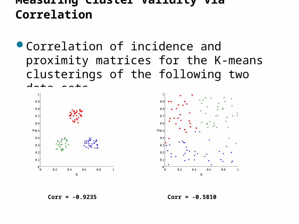
Correlation of incidence and proximity matrices for the K-means clusterings of the following two data sets.
0 0.2 0.4 0.6 0.8 10
0.1
0.2
0.3
0.4
0.5
0.6
0.7
0.8
0.9
1
x
y
0 0.2 0.4 0.6 0.8 10
0.1
0.2
0.3
0.4
0.5
0.6
0.7
0.8
0.9
1
x
y
Corr = -0.9235 Corr = -0.5810
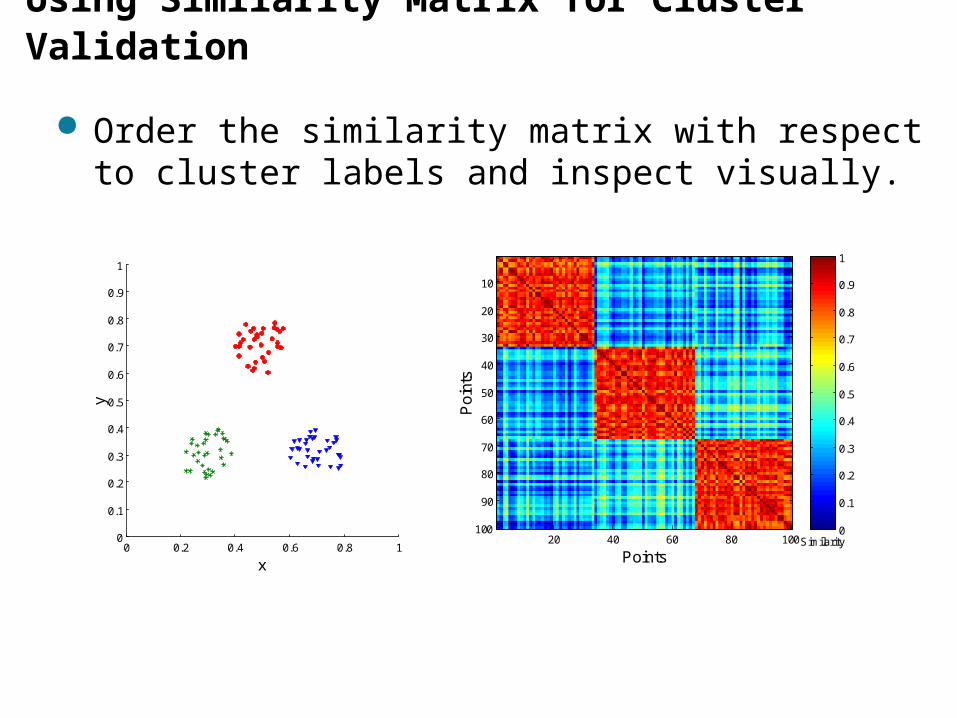
Order the similarity matrix with respect to cluster labels and inspect visually.
Using Similarity Matrix for Cluster Validation
0 0.2 0.4 0.6 0.8 10
0.1
0.2
0.3
0.4
0.5
0.6
0.7
0.8
0.9
1
x
y
Points
Po
ints
20 40 60 80 100
10
20
30
40
50
60
70
80
90
100Similarity
0
0.1
0.2
0.3
0.4
0.5
0.6
0.7
0.8
0.9
1
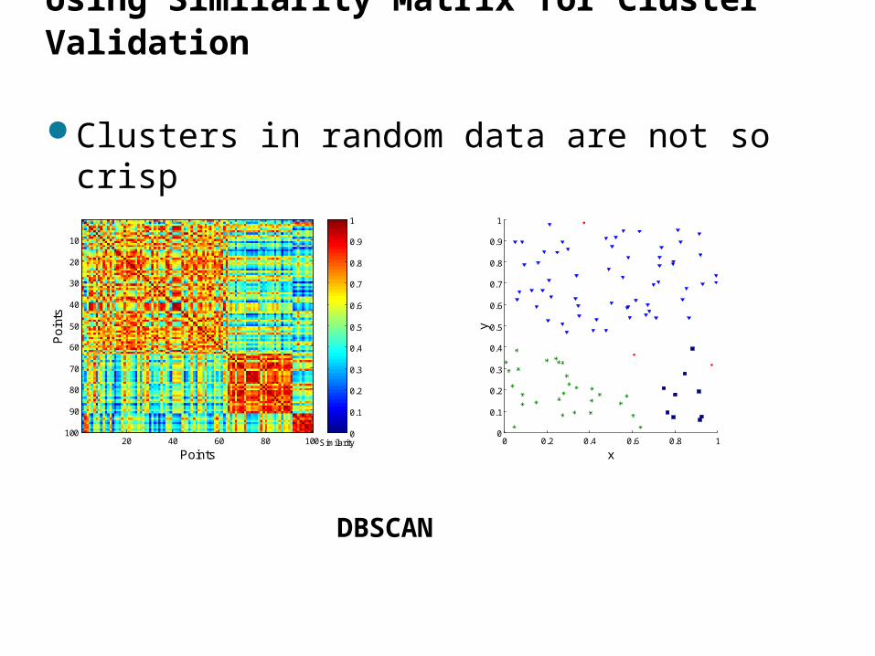
Using Similarity Matrix for Cluster Validation
Clusters in random data are not so crisp
Points
Po
ints
20 40 60 80 100
10
20
30
40
50
60
70
80
90
100Similarity
0
0.1
0.2
0.3
0.4
0.5
0.6
0.7
0.8
0.9
1
DBSCAN
0 0.2 0.4 0.6 0.8 10
0.1
0.2
0.3
0.4
0.5
0.6
0.7
0.8
0.9
1
x
y
Points
Po
ints
20 40 60 80 100
10
20
30
40
50
60
70
80
90
100Similarity
0
0.1
0.2
0.3
0.4
0.5
0.6
0.7
0.8
0.9
1
Using Similarity Matrix for Cluster Validation
Clusters in random data are not so crisp
K-means
0 0.2 0.4 0.6 0.8 10
0.1
0.2
0.3
0.4
0.5
0.6
0.7
0.8
0.9
1
x
y
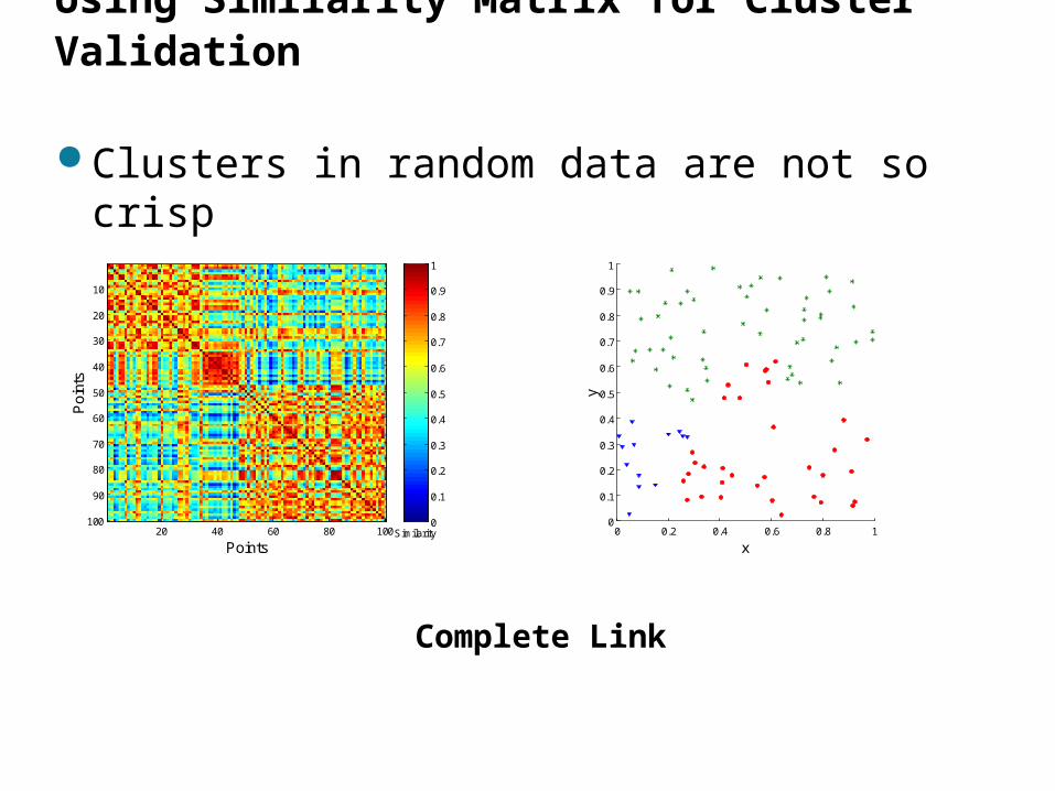
Using Similarity Matrix for Cluster Validation
Clusters in random data are not so crisp
0 0.2 0.4 0.6 0.8 10
0.1
0.2
0.3
0.4
0.5
0.6
0.7
0.8
0.9
1
x
y
Points
Po
ints
20 40 60 80 100
10
20
30
40
50
60
70
80
90
100Similarity
0
0.1
0.2
0.3
0.4
0.5
0.6
0.7
0.8
0.9
1
Complete Link
Using Similarity Matrix for Cluster Validation
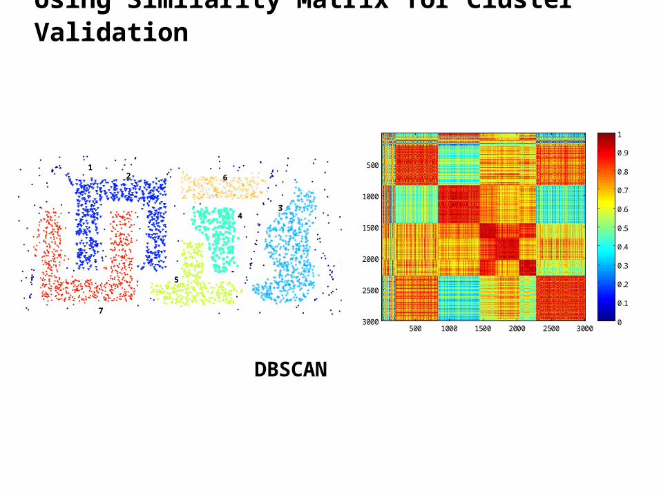
1 2
3
5
6
4
7
DBSCAN
0
0.1
0.2
0.3
0.4
0.5
0.6
0.7
0.8
0.9
1
500 1000 1500 2000 2500 3000
500
1000
1500
2000
2500
3000
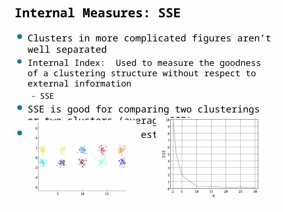
Clusters in more complicated figures aren’t well separated
Internal Index: Used to measure the goodness of a clustering structure without respect to external information– SSE
SSE is good for comparing two clusterings or two clusters (average SSE).
Can also be used to estimate the number of clusters
Internal Measures: SSE
2 5 10 15 20 25 300
1
2
3
4
5
6
7
8
9
10
K
SS
E
5 10 15
-6
-4
-2
0
2
4
6
Internal Measures: SSE
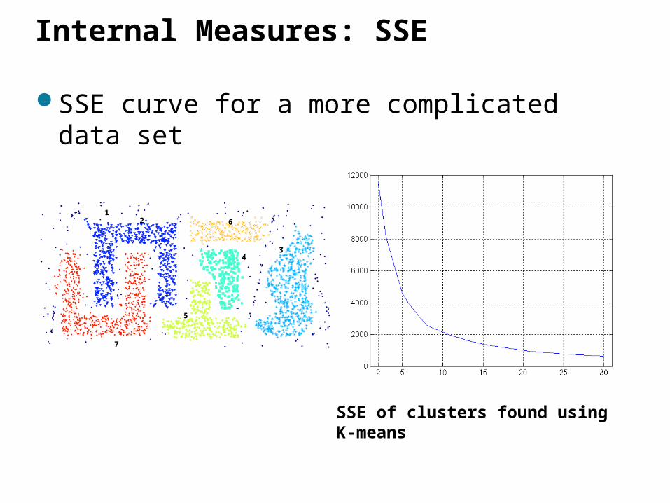
SSE curve for a more complicated data set
1 2
3
5
6
4
7
SSE of clusters found using K-means
Need a framework to interpret any measure. – For example, if our measure of evaluation has the value, 10, is
that good, fair, or poor?
Statistics provide a framework for cluster validity– The more “atypical” a clustering result is, the more likely it
represents valid structure in the data
– Can compare the values of an index that result from random data or clusterings to those of a clustering result.
If the value of the index is unlikely, then the cluster results are valid
– These approaches are more complicated and harder to understand.
For comparing the results of two different sets of cluster analyses, a framework is less necessary.
– However, there is the question of whether the difference between two index values is significant
Framework for Cluster Validity
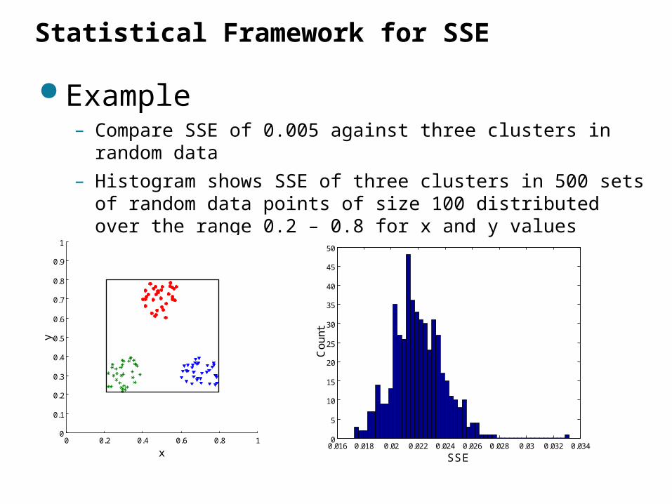
Example– Compare SSE of 0.005 against three clusters in random
data
– Histogram shows SSE of three clusters in 500 sets of random data points of size 100 distributed over the range 0.2 – 0.8 for x and y values
Statistical Framework for SSE
0.016 0.018 0.02 0.022 0.024 0.026 0.028 0.03 0.032 0.0340
5
10
15
20
25
30
35
40
45
50
SSE
Co
unt
0 0.2 0.4 0.6 0.8 10
0.1
0.2
0.3
0.4
0.5
0.6
0.7
0.8
0.9
1
x
y
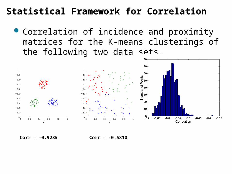
Correlation of incidence and proximity matrices for the K-means clusterings of the following two data sets.
Statistical Framework for Correlation
0 0.2 0.4 0.6 0.8 10
0.1
0.2
0.3
0.4
0.5
0.6
0.7
0.8
0.9
1
x
y
0 0.2 0.4 0.6 0.8 10
0.1
0.2
0.3
0.4
0.5
0.6
0.7
0.8
0.9
1
x
y
Corr = -0.9235 Corr = -0.5810
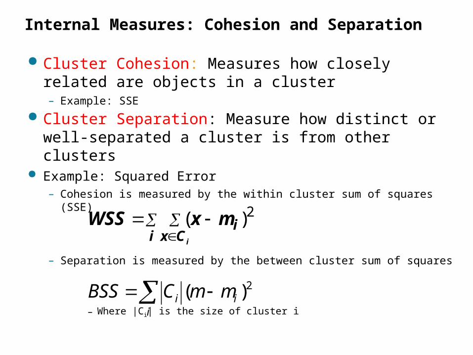
Cluster Cohesion: Measures how closely related are objects in a cluster– Example: SSE
Cluster Separation: Measure how distinct or well-separated a cluster is from other clusters
Example: Squared Error– Cohesion is measured by the within cluster sum of squares
(SSE)
– Separation is measured by the between cluster sum of squares
– Where |Ci| is the size of cluster i
Internal Measures: Cohesion and Separation
i Cx
ii
mxWSS 2)(
i
ii mmCBSS 2)(
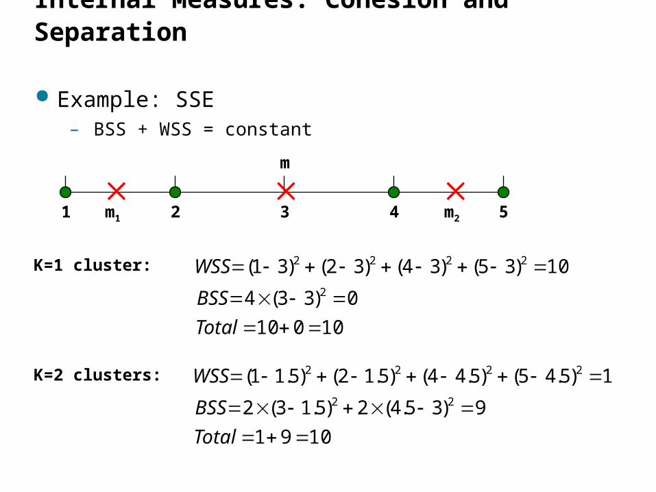
Internal Measures: Cohesion and Separation
Example: SSE– BSS + WSS = constant
1 2 3 4 5 m1 m2
m
1091
9)35.4(2)5.13(2
1)5.45()5.44()5.12()5.11(22
2222
Total
BSS
WSSK=2 clusters:
10010
0)33(4
10)35()34()32()31(2
2222
Total
BSS
WSSK=1 cluster:
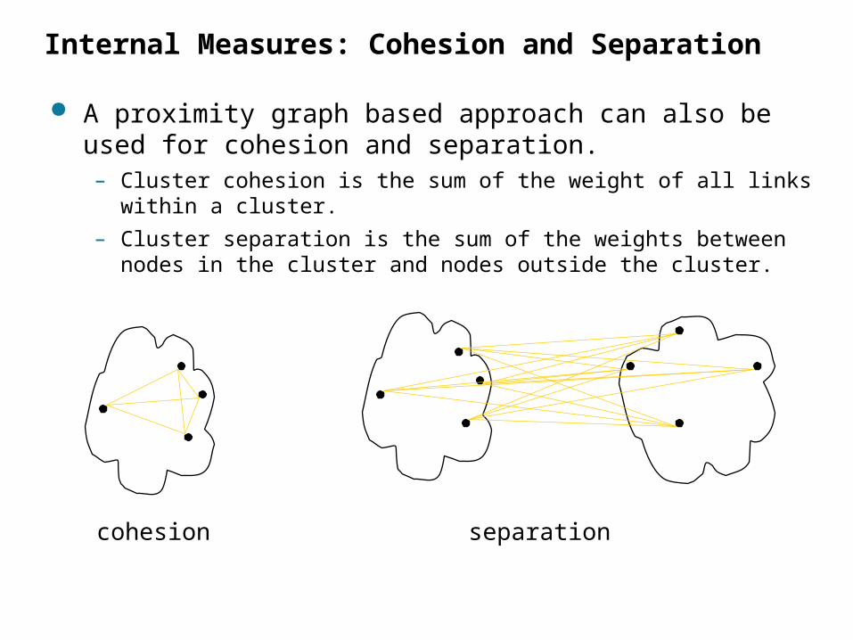
A proximity graph based approach can also be used for cohesion and separation.– Cluster cohesion is the sum of the weight of all links within a
cluster.
– Cluster separation is the sum of the weights between nodes in the cluster and nodes outside the cluster.
Internal Measures: Cohesion and Separation
cohesion separation
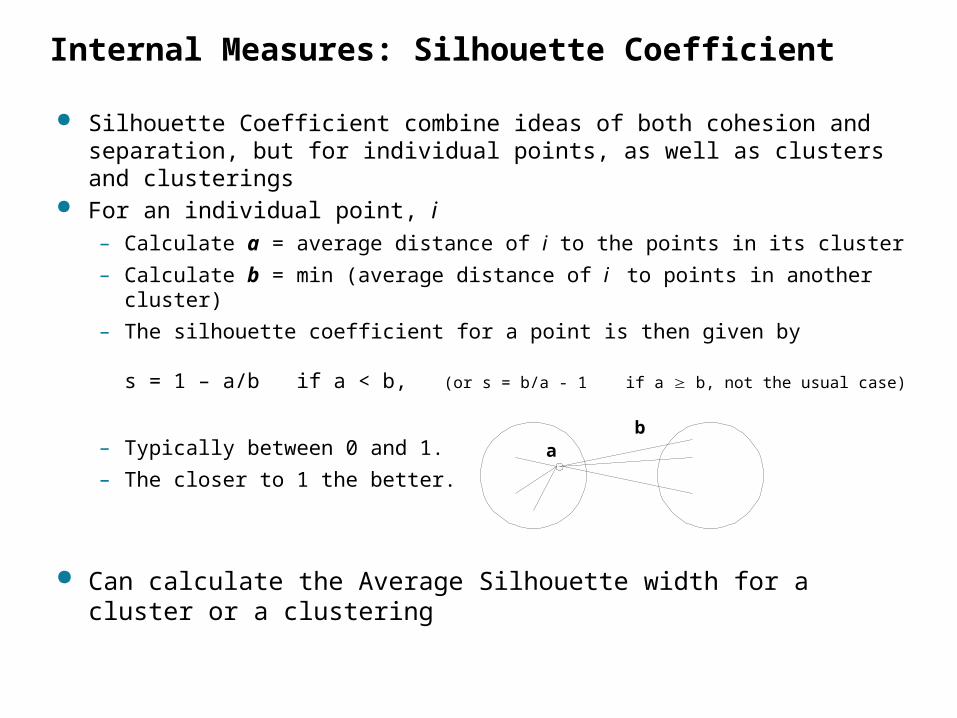
Silhouette Coefficient combine ideas of both cohesion and separation, but for individual points, as well as clusters and clusterings
For an individual point, i– Calculate a = average distance of i to the points in its cluster
– Calculate b = min (average distance of i to points in another cluster)
– The silhouette coefficient for a point is then given by
s = 1 – a/b if a < b, (or s = b/a - 1 if a b, not the usual case)
– Typically between 0 and 1.
– The closer to 1 the better.
Can calculate the Average Silhouette width for a cluster or a clustering
Internal Measures: Silhouette Coefficient
ab
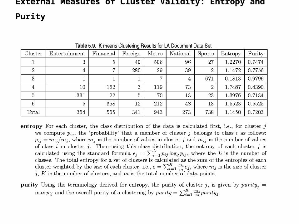
External Measures of Cluster Validity: Entropy and
Purity
“The validation of clustering structures is the most difficult and frustrating part of cluster analysis.
Without a strong effort in this direction, cluster analysis will remain a black art accessible only to those true believers who have experience and great courage.”
Algorithms for Clustering Data, Jain and Dubes
Final Comment on Cluster Validity