Embed Size (px)
Citation preview
UPDATED ENERGY AND EMISSIONS PROJECTIONS 2017
January 2018
UPDATED ENERGY AND EMISSIONS PROJECTIONS 2017
© Crown copyright 2017
You may re-use this information (not including logos) free of charge in any format or
medium, under the terms of the Open Government Licence.
To view this licence, visit www.nationalarchives.gov.uk/doc/open-government-
licence/version/3/ or write to the Information Policy Team, The National Archives, Kew,
London TW9 4DU, or email: [email protected].
Any enquiries regarding this publication should be sent to us at
This publication is available for download at www.gov.uk/government/publications.
2
Contents
Lists of figures and tables ______________________________________________ 4
Executive summary ____________________________________________________ 5
1 Introduction ______________________________________________________ 7
About this document __________________________________________________ 7
The reference case and other scenarios __________________________________ 9
Details of changes to the projections methodology __________________________ 10
2 UK emissions projections ___________________________________________ 12
Comparison to the 2016 projections ______________________________________ 13
Progress towards the carbon budgets ____________________________________ 15
Non-traded emissions projections by sector ________________________________ 19
3 Effect of policies on emissions ______________________________________ 22
Policies for emissions reduction _________________________________________ 22
Changes to emissions savings since EEP 2016 ____________________________ 24
Emissions savings from policies by consumer sector ________________________ 26
Emissions savings from policies in electricity supply _________________________ 27
4 Demand for energy ________________________________________________ 28
Introduction _________________________________________________________ 28
Methodology for demand projections _____________________________________ 29
Final energy demand _________________________________________________ 30
Primary energy demand _______________________________________________ 32
5 Electricity supply __________________________________________________ 34
Summary of projections _______________________________________________ 35
Autogenerators ______________________________________________________ 37
6 Uncertainty in emissions projections _________________________________ 39
Different sources of uncertainty _________________________________________ 39
Parameters considered for uncertainty analysis _____________________________ 41
Structural break uncertainty ____________________________________________ 44
Uncertainties not covered in this analysis__________________________________ 46
Conclusions _________________________________________________________ 46
7 Lists of supporting material _________________________________________ 47
Annexes ___________________________________________________________ 47
Web tables and charts ________________________________________________ 47

Lists of figures and tables
3
Appendix A: List of abbreviations __________________________________________ 48
Lists of figures and tables
4
Lists of figures and tables
Figures
Figure 2.1: Uncertainty in projected overall territorial emissions .............................. 13
Figure 2.2: Actual and projected performance against carbon budgets, MtCO2e ..... 17
Figure 2.3: Non-traded emissions in the economy, MtCO2e .................................... 21
Figure 4.1: Primary and final energy demand .......................................................... 28
Figure 4.2: Final energy demand by fuel and consumer sector 2008 to 2035, Mtoe 30
Figure 4.3: Primary energy demand by fuel, Mtoe ................................................... 33
Figure 5.1: Generation and net imports, TWh .......................................................... 35
Figure 5.2: Emissions intensity (vs EEP 2016), gCO2e/kWh .................................... 36
Figure 5.3: CHP generating capacity, GW ............................................................... 37
Figure 6.1: Total GHG emissions: uncertainty range for each category separately . 43
Tables
Box 1: The UK net carbon account .......................................................................... 16
Table 2.1: Performance against carbon budgets, MtCO2e ....................................... 19
Table 3.1: Non-traded GHG emissions savings from policies, MtCO2e .................... 23
Table 6.1: Categorisation of parameters and variables considered ......................... 41
Table 6.2: Net carbon account for the fourth carbon budget period: uncertainty
ranges by category, MtCO2e .................................................................................... 44
Executive summary
5
Executive summary
Achieving clean growth, while ensuring an affordable energy supply for businesses
and consumers, is at the heart of the UK’s Industrial Strategy.
The UK has been among the most successful countries in the developed world in
growing our economy while reducing emissions, and the recently published Clean
Growth Strategy1 sets out ambitious policies and proposals to meet our carbon
reduction targets while seizing the opportunities of clean growth.
To support our work on clean growth, BEIS produces projections of UK energy
demand and greenhouse gas emissions, currently up to 2035.
The analysis set out in this report shows that the UK’s projected performance against
our carbon budgets has improved. BEIS’s current estimated projection for the fourth
and fifth carbon budgets suggests that we could deliver 97 per cent and 95 per cent
of our required performance against 1990 levels – for carbon budgets which will end
in ten and fifteen years’ time respectively.
The central projections2 detailed in this report include policies which are categorised
as implemented, adopted or planned. Further detail of these categories is given in
Chapter 1. The projections are based on policy analysis from July 2017 and power
sector modelling from September 2017. Potential savings from a subset of policies in
the Clean Growth Strategy are included in Table 2.1 on page 19, and the full impact
of new policies and proposals from the Clean Growth Strategy will be included in
future EEP editions when they are developed more fully3.
Other key projections in the report are that:
• trends in total primary energy demand are similar to the 2016 projections,
falling 11% between 2016 and 2025, from 201 to 179 million tonnes of oil
equivalent (Mtoe), before rising again to 193 Mtoe in 2035.
• in the power sector, the central projection shows greenhouse gas emissions
falling by 53% between 2015 and 2020.
1 Clean Growth Strategy: published in October 2017.
https://www.gov.uk/government/publications/clean-growth-strategy 2 The report and annexes contain outputs from projections under a number of different macro-
economic assumptions. All of these include implemented, adopted and planned policies except the “baseline” projection which projects energy and emissions in the absence of policies, and the “existing policies” projection which excludes planned policies. 3 The Clean Growth Strategy quoted the latest available projections at the time of publication (EEP
2016).

Executive summary
6
The changes to our projections are due to updates to a range of data and
assumptions – these include updates to 2016 actual data on energy demand and
temperature, and the higher assumptions for fossil fuel price projections as
compared to those used in EEP 2016.
As set out in the Clean Growth Strategy, we will in future also track our progress
through annual publication of our Emissions Intensity Ratio.
Introduction
7
1 Introduction
• This report contains projections of performance against UK
greenhouse gas (GHG) targets under existing policies.
• Legally binding carbon budgets are set for five year periods and are
aimed at reducing emissions by at least 80% by 2050.
• Performance against carbon budgets is measured by the net carbon
account (see Box 1 in Chapter 2) and primarily depends on the level
of non-traded emissions. These are emissions not covered by the
European Union Emissions Trading System (EU ETS).
• The carbon budgets periods are: 2008 to 2012 (CB1); 2013 to 2017
(CB2); 2018 to 2022 (CB3); 2023 to 2027 (CB4); and 2028 to 2032
(CB5).
• The fifth carbon budget (CB5) was approved by Parliament in
summer 2016.
• The Government published its Clean Growth Strategy in October
2017.
About this document
Since the late 1970s, the Government has published projections of UK energy
demand and supply, and in the 1990s these were extended to include projected
carbon dioxide (CO2) and other greenhouse gas (GHG) emissions as well. The
Department for Business, Energy & Industrial Strategy (BEIS) is responsible for
publishing these projections annually. This is the latest report in a series, providing
up-to-date projections to 2035.
The main projection is the ‘reference case’, which is one view of how the UK energy
and emissions system could evolve if implemented, adopted and agreed4
Government policies were implemented but no new policies or changes to existing
policies were introduced.
This report sets out the 2017 projections, with a comparison against the projections
published for 2016 (EEP 2016, published in March 2017) and explanations of
differences between these (mainly focusing on changes in the fourth and fifth carbon
4 By agreed policies, we mean policies which are at the point that policy-specific analysis has been
published with sufficient detail for inclusion in the Energy and Emissions Projections (EEP).
Introduction
8
budget periods). The projections bring together statistical and modelled information
from a wide variety of different sources5:
• The main source of energy consumption data is the annual Digest of UK
Energy Statistics (often referred to as DUKES). The most recent full year of
data is 2016 (published July 2017), so all DUKES figures in this report are
quoted against a comparison year of 2016.
• The main source of emissions statistics is the Greenhouse Gas Inventory,
updated each February. The most recent full year of data is 2015, so all
Inventory figures in this report are quoted against a comparison year of 2015.
• To produce these projections, these data sets are combined with economic
data (for example, GDP projections from the Office for Budget Responsibility)
to update equations that project forward energy demand and emissions in the
absence of policy.
The main model used is the Energy Demand Model (EDM), which is a mixed (top
down/bottom up) econometric model of energy demand and combustion related
greenhouse gas (GHG) emissions for the UK economy. It is run in combination with
other BEIS models which model retail electricity prices and the electricity supply
sector.
This generates projections of primary and final energy demand by year, economic
sector and fuel. The following ‘non-energy-related’ GHG emissions are projected by
other Government departments and external bodies and then added to the EDM
projections:
• Emissions from agriculture and waste;
• Emissions from Land Use, Land Use Change and Forestry (LULUCF).
This report helps to assess the UK’s progress towards its own targets for GHG
emissions. The targets were introduced by the 2008 Climate Change Act, which
established a long-term target for the UK to reduce its net emissions in 2050 by at
least 80% compared to 19906. The Act also established a system of legally binding
limits on the net amount of GHGs that can be emitted. These are called carbon
budgets7. Each carbon budget spans five years and is set with a view to keeping the
UK on track to its 2050 target. The UK Parliament approved the level of the fifth
carbon budget8 in summer 2016. Chapter 2 assesses the UK’s progress towards
5 Energy and emissions projections:
https://www.gov.uk/government/collections/energy-and-emissions-projections 6 Compared with a base year of 1990 for CO2, CH4 and N2O, and 1995 for fluorinated gases:
https://www.legislation.gov.uk/ukpga/2008/27/contents 7 See page 142 of the Clean Growth Strategy for more background on carbon budgets:
https://www.gov.uk/government/publications/clean-growth-strategy 8 Fifth carbon budget order: http://www.legislation.gov.uk/uksi/2016/785/made
Introduction
9
these carbon budget obligations and gives an overview of emissions by different
economic sectors.
The UK Government develops and implements policies with the aim of reducing
GHG emissions in line with the carbon budgets and current international
commitments. These projections indicate the broad scale of action that may be
needed to keep emissions within the carbon budgets. This is the subject of Chapter
3. These projections include policies mentioned in the Clean Growth Strategy if they
were classed as implemented, adopted or agreed at the cut-off point of July 2017. In
addition, table 2.1 shows projected performance against carbon budget targets, and
provides an updated version of the Clean Growth Strategy’s summary of
performance against carbon budgets with the initial estimates of new early stage
policies and proposals included. As the range of other policies and proposals are
developed, their impacts will be included as appropriate in future projections.
Emission estimates are underpinned by projections of the future demand for energy.
Chapter 4 sets out final and primary energy use projections to 2035 and includes a
discussion of trends within the key consuming sectors.
Chapter 5 sets out the projections for the electricity sector, and briefly reviews the
influence of this sector’s activity on wider emissions.
Finally, Chapter 6 summarises some of the sources of uncertainty in these
projections. It explains the methodology which was used to estimate the lower and
upper confidence interval for the 2017 Energy and Emissions Projections.
The reference case and other scenarios
The main projection presented in this report is the BEIS ‘reference case’ or central
projection. The reference case is based on central projections for the key drivers of
energy and emissions, such as fossil fuel prices, Gross Domestic Product (GDP) and
population. Projections of emissions outside of the power sector are based on
applying standard statistical techniques to project forward energy demand and
emissions based on trends and relationships identified in past data. These are
adjusted to take account of the estimated impact of implemented, adopted and
agreed (as at July 2017) Government policies.
Electricity demand is also projected forward using statistical techniques and adjusted
for the impact of existing policies that impact on electricity demand. However, the
projection of electricity generation is based on a model of supplier behaviour rather
than statistical analysis of past trends. It also only reflects current policy up to 2020.
Beyond 2020, the electricity generation scenario includes assumptions that go
Introduction
10
beyond current Government policy, and is therefore illustrative. The reference
electricity generation scenario therefore represents one particular view of how the
system could evolve and is not a forecast or preferred scenario.
Chapter 3 discusses policy impacts on emissions, and for this the ‘reference’
scenario is compared against a ‘baseline’ scenario which excludes the impact of all
climate change policies brought in since the 2009 Low Carbon Transition Plan9
(LCTP).
Besides the reference and baseline scenarios, the annexes to this report also set out
the following additional scenarios:
• low and high fossil fuel price scenarios;
• low and high economic growth scenarios;
• an ‘existing policies’ scenario which only includes policies that have been
implemented or adopted (but not planned policies).
For all these scenarios, other views of the future are possible and there are
significant uncertainties in these projections. Some of this uncertainty is captured in
our projections modelling and presented in this report, but not all of it (see Chapter
6).
Details of changes to the projections methodology
Since the EEP 2016 projections (published in March 2017), the BEIS modelling team
have concentrated on updates to the projections methodology and quality
assurance. In particular, improvements were made to Combined Heat and Power
(CHP) modelling and the calculation of traded shares. As in all years, the model was
updated to use the most recent actual emissions data (2015 inventory10), energy
statistics (DUKES) and the macro-economic projections available at the time the
projections were calculated.
The methodological and reporting changes in the 2017 projections are:
9 The Low Carbon Transition Plan publication is available at:
https://www.gov.uk/government/publications/the-uk-low-carbon-transition-plan-national-strategy-for-climate-and-energy 10
EEP 2017 uses historic (inventory) GHG emissions data to 2015 and projected emissions from 2016.
Introduction
11
• Modelling of Combined Heat and Power (CHP) plants has been incorporated
within BEIS’s “Dynamic Dispatch Model” of the wider power supply sector11. CHP
had previously been projected using a separate model. The new approach
enables projections to be made in the context of the whole electricity market and
facilitates projections beyond 2030. It also ensures that interactions between
CHP and the wider power sector are taken into account.
• Final energy demand (Annex F) no longer includes fuel used to make heat which
is sold as steam or hot water (for example, by CHP plants).12 Primary energy
demand (Annex E) continues to include fuel used for heat generation. This
contributes around 1.4% of primary energy in 2020.
• The methodology for calculating the proportion of UK emissions traded under the
EU Emissions Trading System (EU ETS) has been modified so that a consistent
approach is used across all policies. Previously the method used bespoke
estimates of the ‘traded share’ of future emissions savings for individual policies.
Under this approach it had not been possible for all policy teams to calculate
impacts in a way consistent between policies and with the EEP reporting
methodology. Direct traded and non-traded emissions savings for all policies are
now estimated jointly as part of the EEP production process, and are projected
forward in each industrial subsector assuming a constant split between the traded
and non-traded sectors, using latest evidence on current proportions. This means
they are now consistent with EU ETS verified emissions.
• In previous years’ EEPs all power station emissions were projected as traded
under the EU ETS. This year, projections of emissions from ‘Energy from Waste’
power plants (which burn municipal waste) are accounted for as ‘non-traded’.
• The EU ETS carbon price has now been included in the industry sector of the
model and the equations of the minerals and chemicals sectors have been
improved. This was undertaken with the help of the analytical experts at
University College London (UCL) who carried out the improvements in early
201713.
We are continually working to improve our projections. In 2018 we intend to share
more details of the methodology.
11
For detail on the DDM see: https://www.gov.uk/government/publications/dynamic-dispatch-model-ddm 12
This aligns with the treatment of heat in DUKES classification (table 1.1) which lists ‘heat generation’ under ‘Transformation’ rather than ‘Final consumption’. 13
The paper is available online at : http://www.sciencedirect.com/science/article/pii/S0140988317302943?_rdoc=1&_fmt=high&_origin=gateway&_docanchor=&md5=b8429449ccfc9c30159a5f9aeaa92ffb&ccp=y
UK emissions projections
12
2 UK emissions projections
• By 2020, emissions are projected to be 50% below 1990 levels
in the reference case (assuming implemented, adopted and
agreed policies).
• The UK met the first carbon budget with headroom of 36
MtCO2e, and is projected to meet the second and third carbon
budgets with headroom of 125 and 143 MtCO2e, respectively.
• There are projected shortfalls against the fourth and fifth carbon
budgets. As policies and proposals in the Clean Growth Strategy
are developed more fully, their impacts will be included as
appropriate in future EEP editions.
• In EEP 2017, emissions are projected to be 3.6% lower in total
over the period 2017 to 2035, compared to EEP 2016
projections. The main reason for this is the updated data for key
inputs such as energy demand and temperature and fossil fuel
price projections.
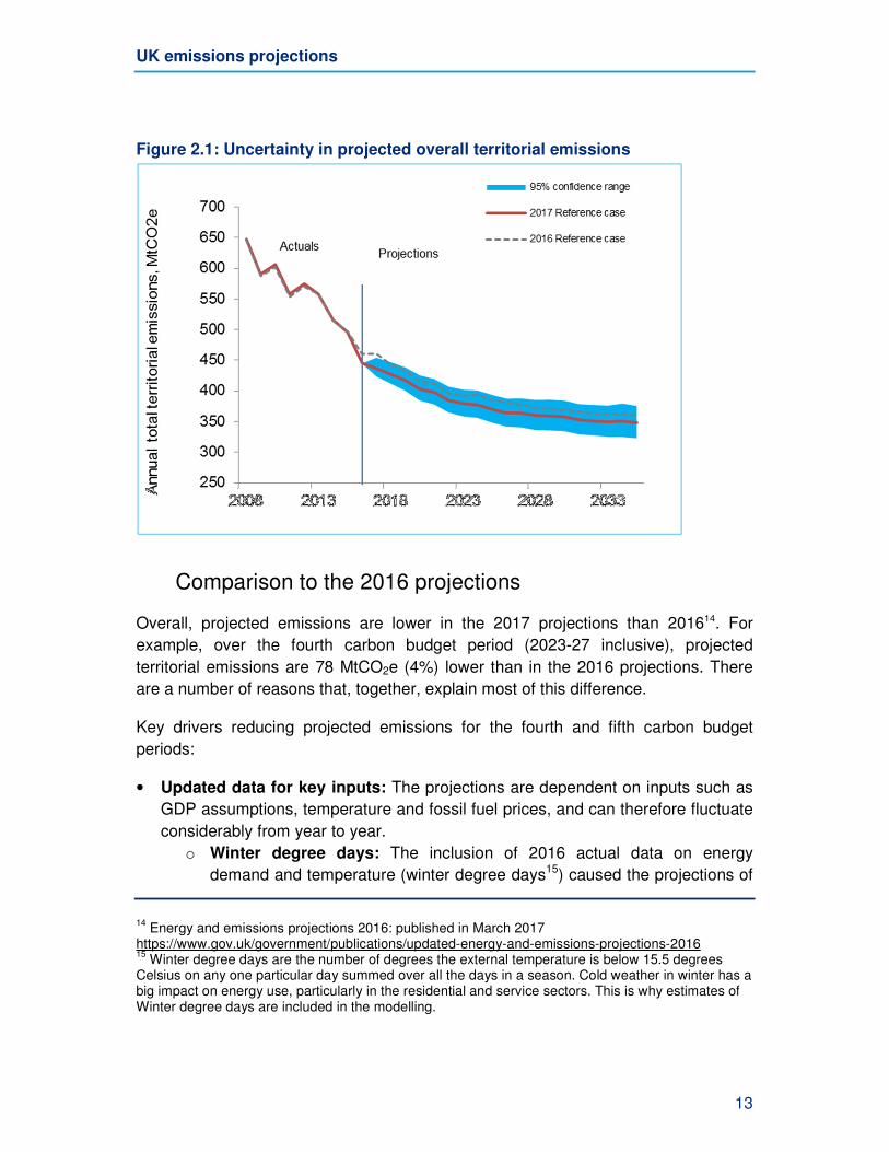
Figure 2.1 shows actual and projected UK territorial emissions. These projections
are very uncertain. For example, societal and behavioural trends and breakthrough
technologies could have profound impacts on our energy mix and emissions, but are
impossible to fully anticipate.
Some of this uncertainty is captured in our projections modelling, but not all of it. The
uncertainty we have been able to model is shown as a fan chart around the central
reference case projections, and is higher for the later years. Chapter 6 discusses
different sources of uncertainty, how this is captured in the projections modelling,
and the methodology used for uncertainty analysis.
UK emissions projections
13
Figure 2.1: Uncertainty in projected overall territorial emissions
Comparison to the 2016 projections
Overall, projected emissions are lower in the 2017 projections than 201614. For
example, over the fourth carbon budget period (2023-27 inclusive), projected
territorial emissions are 78 MtCO2e (4%) lower than in the 2016 projections. There
are a number of reasons that, together, explain most of this difference.
Key drivers reducing projected emissions for the fourth and fifth carbon budget
periods:
• Updated data for key inputs: The projections are dependent on inputs such as
GDP assumptions, temperature and fossil fuel prices, and can therefore fluctuate
considerably from year to year.
o Winter degree days: The inclusion of 2016 actual data on energy
demand and temperature (winter degree days15) caused the projections of
14
Energy and emissions projections 2016: published in March 2017 https://www.gov.uk/government/publications/updated-energy-and-emissions-projections-2016 15
Winter degree days are the number of degrees the external temperature is below 15.5 degrees Celsius on any one particular day summed over all the days in a season. Cold weather in winter has a big impact on energy use, particularly in the residential and service sectors. This is why estimates of Winter degree days are included in the modelling.
UK emissions projections
14
future heating requirements to be revised downward for domestic and
services energy demand.
o Fossil fuel prices: For the residential and industry sectors, emissions
have reduced due to the higher assumptions for fossil fuel prices
compared to those used in EEP 2016. Higher fossil fuel prices generally
have an effect of dampening energy demand.
Some less significant drivers which slightly increase projected emissions for the
fourth and fifth carbon budget periods:
• Iron and Steel: Compared to EEP 2016, emissions in the Iron and Steel sector
are projected to rise by 8 MtCO2e in the fourth carbon budget period. This is due
to improved projections processes, which corrected a potential misalignment
affecting this sector in EEP 2016.
• Land Use, Land Use Change and Forestry (LULUCF): Compared to EEP 2016
there is a slight decrease in the projected removals of greenhouse gases due to
LULUCF. This is due to updated modelling of forest carbon stocks in soils and
litter and new data on settlement expansion which have been used to revise the
model. This also affects historical years.
Key drivers which shifted the classification of some emissions include:
• Energy from waste: In previous editions of EEP, all power station emissions
were projected as traded under the EU ETS. This year, projections of emissions
from ‘Energy from Waste’ power plants are now accounted for as ‘non-traded’,
bringing this into line with the ETS directive16. This resulted in a shift of 11
MtCO2e of power sector emissions from the traded to non-traded sector for the
fourth carbon budget period.
• Allocation of policy savings to traded sector: To produce projections of the
net carbon account and hence progress against carbon budgets, the EEP
apportions industry and services emissions into traded and non-traded for
reporting purposes. An improvement in the methodology this year17 led, in
general, to a higher allocation of policy savings to the traded sector than to the
non-traded sector. The new methodology aims to provide improved aggregated
policy savings and is now based on historic EU ETS data18. However since it is
16
See annex I of the ETS directive, available at http://eur-lex.europa.eu/legal-content/EN/TXT/PDF/?uri=CELEX:02003L0087-20140430&from=EN. 17
Traded share estimates for policies had previously been provided by policy experts, however, the average traded share of the sector, based on historic verified EU ETS data, is now used. 18
Traded share estimates for policies had previously been provided by policy experts, however, the average traded share of the sector, based on historic verified EU ETS data, is now used.
UK emissions projections
15
not tailored to each specific policy, sector splits may not match those presented
in individual policy impact assessments.
Progress towards the carbon budgets
The Energy and Emissions Projections are one measure of the UK’s progress
towards future targets for GHG emissions. The 2008 Climate Change Act
established a long-term target for the UK to reduce its net emissions in 2050 by at
least 80% compared to 199019. The Act also established a system of legally-binding
carbon budgets which limit the net amount of GHGs that can be emitted in
successive five-year periods, starting in 200820.
The first carbon budget covered the period 2008 to 2012 and the UK met this budget
with headroom of 36 MtCO2e. Budget levels have been set for four further periods:
2013 to 2017 inclusive, 2018 to 2022, 2023 to 2027, and 2028 to 2032.
In 2016, the Government set the level of the fifth carbon budget (2028-32) in
agreement with advice from the Committee on Climate Change, at a level of 1,725
MtCO2e, equivalent to an average 57% reduction on 1990 emissions.
In October 2017, the Government published its Clean Growth Strategy, setting out
policies and proposals for meeting future carbon budgets and illustrative pathways
for the 2050 target21. Table 2.1 shows projected performance against carbon budget
targets, and provides an updated version of the Clean Growth Strategy’s summary of
performance against carbon budgets22 with the initial estimates of new early stage
policies and proposals included.
19
Compared with a base year of 1990 for CO2, CH4 and N2O, and 1995 for fluorinated gases: https://www.theccc.org.uk/publication/building-a-low-carbon-economy-the-uks-contribution-to-tackling-climate-change-2/ 20
For more details on the UK’s climate change targets, including the carbon budgets, see: https://www.gov.uk/guidance/carbon-budgets 21
Clean Growth Strategy: published in October 2017. https://www.gov.uk/government/publications/clean-growth-strategy 22
The Clean Growth Strategy quoted the latest available projections at the time of publication (EEP 2016). Emissions projections from the Clean Growth Strategy are therefore not directly comparable to the projections within this report.
UK emissions projections
16
On 23 June 2016, the EU referendum took place and the people of the United
Kingdom voted to leave the European Union. Until the date of exit, the UK remains a
full member of the European Union and all the rights and obligations of EU
membership remain in force. While exit negotiations remain in progress, the Energy
and Emissions Projections are produced on that basis.
Performance against carbon budgets is measured by the UK net carbon account –
described in Box 1. Figure 2.2 and Table 2.1 show the actual and projected
performance against legislated carbon budgets. The range presented in the
projected net carbon account is the 95% confidence interval for uncertainties that
have been modelled. Chapter 6 gives more details on how this uncertainty analysis
was carried out, and Table 6.1 summarises the variables considered in this
uncertainty analysis. This does not capture all sources of uncertainty or the full range
in uncertainty (discussed in Chapter 6).
Box 1: The UK net carbon account
Compliance with the budgets is assessed by comparing the UK “net carbon account”1
(NCA) against the carbon budget level. The NCA is currently defined as the sum of three
components: 1) emissions allowances allocated to the UK under the EU Emissions
Trading System (EU ETS), 2) UK emissions not covered by the EU ETS; 3) credits/debits
from other international crediting systems.
1. Emissions covered by the EU ETS, or “traded sector emissions” generally include
those from power generation and from large energy-intensive industrial plants. For
the net carbon account, traded sector emissions are measured as the UK’s
allocation of allowances under the EU ETS. To project future carbon budget
performance the level of allocation must be estimated. The levels used are based
on the assumed shares at the time of setting the respective carbon budgets, as
the UK’s actual future shares are not fully known at this stage. Projections for the
actual level of allocation covered by the EU ETS can be found in the web tables.
2. “Non-traded emissions” include all UK GHG emissions which are not covered by
the emissions trading system (EU ETS). For example, this includes road transport,
heating in buildings, agriculture, waste and some industry. For EEP 2017,
projections of emissions from ‘Energy from Waste’ power plants are now
accounted for as ‘non-traded’, bringing this into line with the ETS directive1.The
UK net carbon account reflects the actual emissions from the UK in those sectors.
3. Credits/debits are also included from other international credit systems.
UK emissions projections
17
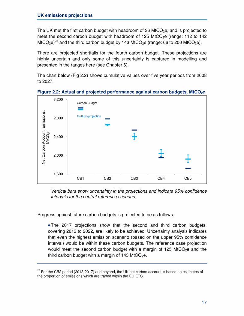
The UK met the first carbon budget with headroom of 36 MtCO2e, and is projected to
meet the second carbon budget with headroom of 125 MtCO2e (range: 112 to 142
MtCO2e)23 and the third carbon budget by 143 MtCO2e (range: 66 to 200 MtCO2e).
There are projected shortfalls for the fourth carbon budget. These projections are
highly uncertain and only some of this uncertainty is captured in modelling and
presented in the ranges here (see Chapter 6).
The chart below (Fig 2.2) shows cumulative values over five year periods from 2008
to 2027.
Figure 2.2: Actual and projected performance against carbon budgets, MtCO2e
Vertical bars show uncertainty in the projections and indicate 95% confidence
intervals for the central reference scenario.
Progress against future carbon budgets is projected to be as follows:
• The 2017 projections show that the second and third carbon budgets,
covering 2013 to 2022, are likely to be achieved. Uncertainty analysis indicates
that even the highest emission scenario (based on the upper 95% confidence
interval) would be within these carbon budgets. The reference case projection
would meet the second carbon budget with a margin of 125 MtCO2e and the
third carbon budget with a margin of 143 MtCO2e.
23
For the CB2 period (2013-2017) and beyond, the UK net carbon account is based on estimates of the proportion of emissions which are traded within the EU ETS.
Carbon Budget
Outturn/projection
1,600
2,000
2,400
2,800
3,200
CB1 CB2 CB3 CB4 CB5
Ne
t C
arb
on
Accoun
t: E
mis
sio
ns,
MtC
O2e
UK emissions projections
18
• For the fourth carbon budget (2023 to 2027), the UK’s emissions are currently
projected to be greater than the cap set by the budget, so a shortfall remains
against this target. Taking into account the uncertainty around the projections,
this shortfall could be as low as 23 MtCO2e or as high as 180 MtCO2e24.
However the size of this shortfall has reduced since the 2016 projections: in the
2016 projections, the reference case shortfall was 146 MtCO2e, but this has
fallen to 94 MtCO2e.
• Many policies which will affect the 2020s and beyond have not yet been
developed to the point at which they can be included in these projections25.
In October 2017, the Government published its Clean Growth Strategy, setting out
policies and proposals for meeting future carbon budgets and illustrative pathways
for the 2050 target26. Table 2.1 provides an updated version of the Clean Growth
Strategy’s summary of performance against carbon budgets27 with the initial
estimates of a subset of new early stage policies and proposals included.
The Clean Growth Strategy used the latest available projections at the time of
publication (EEP 2016). Projected performance against carbon budgets has
improved compared to the EEP 2016 projections. The gap between projected
performance and targets (before Clean Growth Strategy policies and proposals) has
narrowed by 52, 53 and 51 MtCO2e in the third, fourth and fifth carbon budgets
respectively, before new policies from the Clean Growth Strategy are taken into
account.
The updated projections for the fourth and fifth carbon budgets (including estimates
of emission reductions from a subset of Clean Growth Strategy policies and
proposals) suggests that we could deliver 97 per cent and 95 per cent of our
required performance against 1990 levels – for carbon budgets which will end in ten
and fifteen years’ time respectively. As policies and proposals in the Clean Growth
Strategy are developed more fully, their impacts will be included as appropriate in
future EEP editions.
24
In the 2016 projections this fourth carbon budget period shortfall was projected to be between 103 and 236 MtCO2e. 25
Within the main EEP projections, policies are included if they are either currently implemented or firmly planned in the future i.e. policies which are still under development are not included. 26
Clean Growth Strategy: published in October 2017. https://www.gov.uk/government/publications/clean-growth-strategy 27
The Clean Growth Strategy quoted the latest available projections at the time of publication (EEP 2016). Emissions projections from the Clean Growth Strategy are therefore not directly comparable to the projections within this report.
UK emissions projections
19
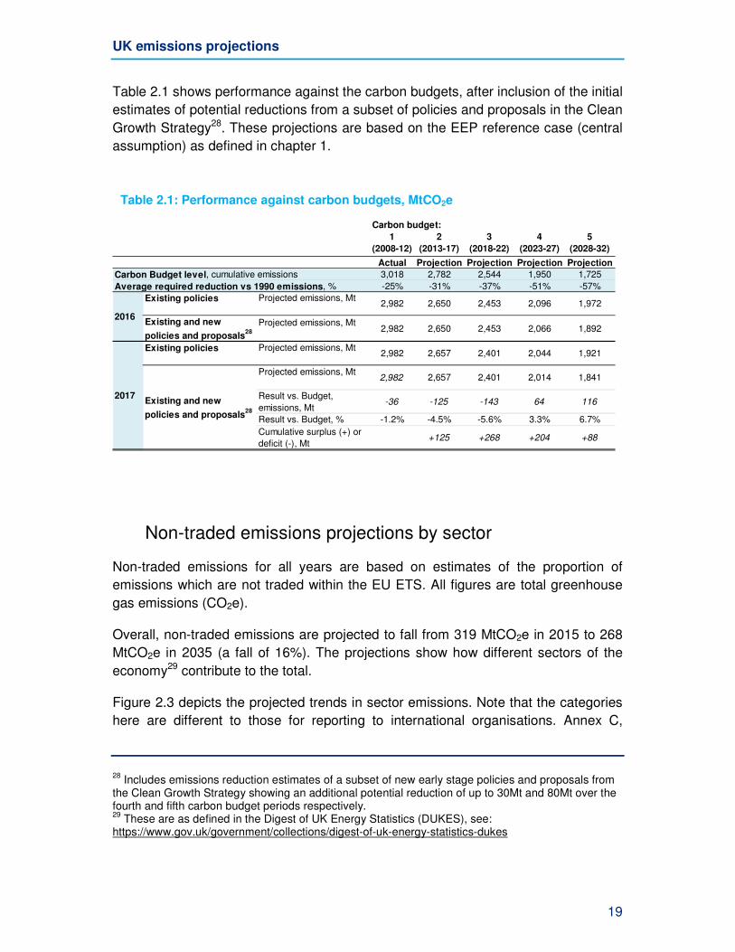
Table 2.1 shows performance against the carbon budgets, after inclusion of the initial
estimates of potential reductions from a subset of policies and proposals in the Clean
Growth Strategy28. These projections are based on the EEP reference case (central
assumption) as defined in chapter 1.
Table 2.1: Performance against carbon budgets, MtCO2e
Carbon budget:
1
(2008-12)
2
(2013-17)
3
(2018-22)
4
(2023-27)
5
(2028-32)
Actual Projection Projection Projection Projection
3,018 2,782 2,544 1,950 1,725
-25% -31% -37% -51% -57%
Existing policies Projected emissions, Mt2,982 2,650 2,453 2,096 1,972
Existing and new
policies and proposals28
Projected emissions, Mt2,982 2,650 2,453 2,066 1,892
Existing policies Projected emissions, Mt2,982 2,657 2,401 2,044 1,921
Projected emissions, Mt2,982 2,657 2,401 2,014 1,841
Result vs. Budget,
emissions, Mt-36 -125 -143 64 116
Result vs. Budget, % -1.2% -4.5% -5.6% 3.3% 6.7%
Cumulative surplus (+) or
deficit (-), Mt+125 +268 +204 +88
Carbon Budget level, cumulative emissions
Average required reduction vs 1990 emissions, %
Existing and new
policies and proposals28
2017
2016
Non-traded emissions projections by sector
Non-traded emissions for all years are based on estimates of the proportion of
emissions which are not traded within the EU ETS. All figures are total greenhouse
gas emissions (CO2e).
Overall, non-traded emissions are projected to fall from 319 MtCO2e in 2015 to 268
MtCO2e in 2035 (a fall of 16%). The projections show how different sectors of the
economy29 contribute to the total.
Figure 2.3 depicts the projected trends in sector emissions. Note that the categories
here are different to those for reporting to international organisations. Annex C,
28
Includes emissions reduction estimates of a subset of new early stage policies and proposals from the Clean Growth Strategy showing an additional potential reduction of up to 30Mt and 80Mt over the fourth and fifth carbon budget periods respectively. 29
These are as defined in the Digest of UK Energy Statistics (DUKES), see: https://www.gov.uk/government/collections/digest-of-uk-energy-statistics-dukes
UK emissions projections
20
“Carbon dioxide emissions by IPCC category”, contains values and definitions for
these.
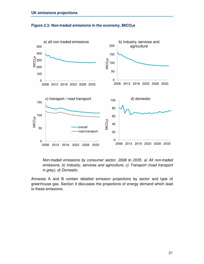
Industry30, commercial services and public administration, agriculture and
waste contributed around 38% of non-traded emissions in 2015. This is projected to
fall to around 31% by 2035.
Land Use, Land Use Change and Forestry (LULUCF) emissions are accounted for
in carbon budgets. They include both sources and sinks31 of greenhouse gases from
forest land, cropland, grassland, human settlements and due to changes of land use
between any of these categories32. LULUCF is currently a sink for atmospheric CO2
but a source of other greenhouse gases – notably nitrous oxide caused by changes
in soil decomposition following the disturbance of soil in land conversion. In 2015,
this sector removed around 1.5% of total greenhouse gas emissions. This figure is
projected to remain at 1.5% in 2035. Further information on non-CO2 emissions from
LULUCF can be found in Annex N of this report.
Transport, mostly road transport, contributed around 40% of UK non-traded
emissions in 2015 (Figure 1.2c). The projections show a decline to 2035 (emissions
are projected to fall by 15% from 2016 levels).
The domestic residential sector (Figure 1.2d) was responsible for 21% of non-
traded emissions in 2015. All emissions from this sector are non-traded. In
comparison to 2015 levels, they are projected to rise by 8 MtCO2e (11%) by 2035,
and will then account for 28% of non-traded emissions.
In past editions of the EEP all power sector emissions were considered traded but
for EEP 2017 emissions from ‘Energy from Waste’ (municipal waste) were excluded
from the traded sector in line with ETS directive 2003/87/EC. These are projected to
account for 2.4 MtCO2e (0.9% of total non-traded emissions) in 2035.
30
This includes CO2 emissions from agriculture due to the burning of fuels and fertiliser use. 31
Carbon sinks are elements of the carbon system that absorb or store carbon dioxide, for example the forests and oceans. 32
A detailed discussion of the components of LULUCF is available here: http://www.ipcc-nggip.iges.or.jp/public/gpglulucf/gpglulucf_files/GPG_LULUCF_FULL.pdf
UK emissions projections
21
Figure 2.3: Non-traded emissions in the economy, MtCO2e
Non-traded emissions by consumer sector, 2008 to 2035. a) All non-traded
emissions, b) Industry, services and agriculture, c) Transport (road transport
in grey), d) Domestic.
Annexes A and B contain detailed emission projections by sector and type of
greenhouse gas. Section 4 discusses the projections of energy demand which lead
to these emissions.
0
100
200
300
400
500
2008 2013 2018 2023 2028 2033
a) all non-traded emissions
MtC
O2e
0
50
100
150
200
2008 2013 2018 2023 2028 2033
MtC
O2e
b) industry, services and agriculture
0
50
100
150
2008 2013 2018 2023 2028 2033
MtC
O2e
c) transport / road transport
overall
road transport
0
20
40
60
80
100
2008 2013 2018 2023 2028 2033
MtC
O2e
d) domestic
Effect of policies on emissions
22
3 Effect of policies on emissions
• Government policies are projected to reduce non-traded GHG emissions. The projected reduction in the fourth carbon budget period is 290 MtCO2e (or about 21% of non-traded emissions in that period).
• About four fifths (81%) of the reduction in non-traded GHG emissions during the fourth carbon budget period comes from policies adopted after the Low Carbon Transition Plan (LCTP) of 2009. The remainder is from policies adopted before the LCTP.
• Overall projected policy savings in the non-traded sector are 7 MtCO2e higher than in EEP 2016 during the fourth carbon budget period due to changes in evidence, assumptions and policies. For the fifth carbon budget period, non-traded policy savings are 16 MtCO2e higher than in EEP 2016.
Policies for emissions reduction
This chapter looks at the impact of Government policies that directly influence
energy use and emissions. Government estimates individual policy impacts by
comparing modelled emissions from scenarios which contain a policy, against
scenarios which do not. The savings from some policies cannot currently be explicitly
identified, particularly in the agriculture and waste management sectors. Although
not separately identifiable, these policy savings are included in the baseline, and are
therefore captured in the projections. Descriptions of some policies for which GHG
savings have not been quantified are given in Annex D.
These projections include policies mentioned in the Clean Growth Strategy only if
they were classed as implemented, adopted or agreed at the cut-off point of July
2017. In addition the Clean Growth Strategy included an initial estimate of the
savings from a further subset of planned policies showing savings of 30 MtCO2e
during the fourth carbon budget period and 80 MtCO2e during the fifth carbon budget
period. As the policies and proposals in the Clean Growth Strategy are further
developed, their impacts will be included as appropriate in future EEP editions.
This chapter focuses on policies that produce savings in the non-traded sector since
they contribute to meeting the carbon budgets (see Chapter 2, Box 1). It also
includes a discussion of the Government policies which reduce emissions from
Effect of policies on emissions
23
electricity generation. The coverage for both traded and non-traded sectors includes
all policies consistent with UNFCCC definitions, as explained on the notes tab of
Annex D33.
For this analysis, policies are grouped according to whether they were adopted
before or after the Low Carbon Transition Plan (LCTP) of 2009. This was the UK’s
first comprehensive plan for moving to a low carbon economy.
Within this chapter, the savings refer only to policies adopted after the LCTP unless
otherwise stated; estimates for these are more robust than for policies adopted
before the LCTP.
Modelling of policy effects is updated regularly and any changes to assumptions will
be incorporated in due course.
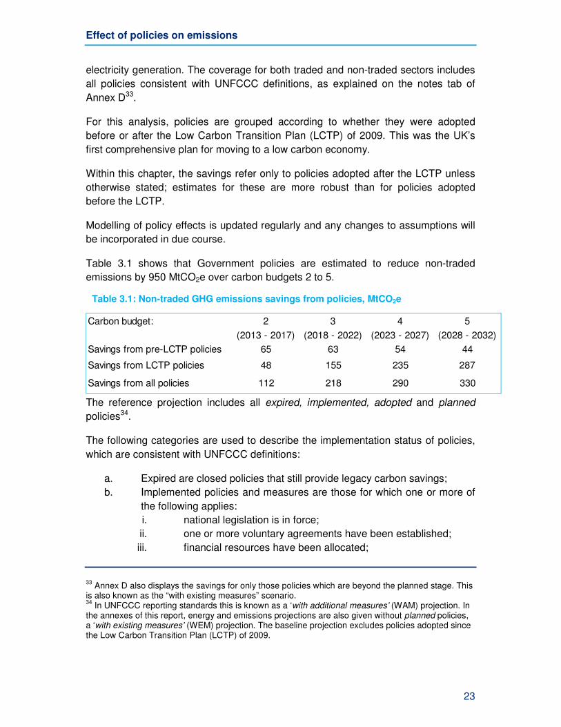
Table 3.1 shows that Government policies are estimated to reduce non-traded
emissions by 950 MtCO2e over carbon budgets 2 to 5.
Table 3.1: Non-traded GHG emissions savings from policies, MtCO2e
The reference projection includes all expired, implemented, adopted and planned
policies34.
The following categories are used to describe the implementation status of policies,
which are consistent with UNFCCC definitions:
a. Expired are closed policies that still provide legacy carbon savings;
b. Implemented policies and measures are those for which one or more of
the following applies:
i. national legislation is in force;
ii. one or more voluntary agreements have been established;
iii. financial resources have been allocated;
33
Annex D also displays the savings for only those policies which are beyond the planned stage. This is also known as the “with existing measures” scenario. 34
In UNFCCC reporting standards this is known as a ‘with additional measures’ (WAM) projection. In the annexes of this report, energy and emissions projections are also given without planned policies, a ‘with existing measures’ (WEM) projection. The baseline projection excludes policies adopted since the Low Carbon Transition Plan (LCTP) of 2009.
Carbon budget: 2 3 4 5
(2013 - 2017) (2018 - 2022) (2023 - 2027) (2028 - 2032)
Savings from pre-LCTP policies 65 63 54 44
Savings from LCTP policies 48 155 235 287
Savings from all policies 112 218 290 330
Effect of policies on emissions
24
iv. human resources have been mobilised.
c. Adopted policies and measures are those for which an official
Government decision has been made and there is a clear commitment to
proceed with implementation.
d. Planned policies and measures are options under discussion and having
a realistic chance of being adopted and implemented in future.
Changes to emissions savings since EEP 2016
Non-traded GHG savings from Government policies are projected to be slightly
higher in the 2017 projections (in comparison to EEP 2016) for all years after 2020.
In the third carbon budget, policy savings reduced slightly from 219 to 218 MtCO2e,
but in the fourth carbon budget, savings increased from 283 to 290 MtCO2e (in
comparison to EEP 2016), and for the fifth carbon budget, savings rose from 314 to
330 MtCO2e.
There are a number of reasons that together explain most of this change.
Key drivers increasing projected non-traded emissions savings from policies:
Transport efficiency policies: The reported savings provided by car fuel efficiency
and electrification policies are higher in these projections than in EEP 2016. Non-
traded savings from car efficiency policies are 58 MtCO2e in the fourth carbon
budget period compared to 42 MtCO2e in EEP 2016. The main reason for this
change is the removal of electric cars from the baseline to simplify analysis and align
with the approach taken by the Committee on Climate Change. There is a further
relatively small increase in savings resulting from higher projections of electric car
usage compared to EEP 2016.
Products policy: More energy-efficient products lead to significant electricity
savings but also result in a Heat Replacement Effect (HRE), requiring an increase in
heating and gas consumption in order to maintain the same level of
temperature. Compared to EEP 2016, the increase in non-traded emissions
attributed to products policy is 4 MtCO2e lower in the fourth carbon budget period
and traded emission savings are 9 MtCO2e lower over the same period. The update
reflects improved evidence and updated assumptions, including to the modelling of
the Heat Replacement Effect (HRE).
Key drivers reducing projected emissions savings from policies:
Traded share methodology change: To produce projections of the net carbon
account and hence progress against carbon budgets, the EEP apportions industry
and services emissions into traded and non-traded for reporting purposes. Traded
Effect of policies on emissions
25
share estimates for policy savings had previously been provided by policy experts
while in EEP 2017 we have used the average traded share of the sector, based on
historic verified EU ETS data. The new methodology aims to provide improved
aggregated policy savings. However since it is not tailored to each specific policy,
sector splits may not match those presented in individual policy impact assessments.
This has led, in general, to a higher allocation of policy savings to the traded sector
than to the non-traded sector compared to EEP 2016. This means that savings
estimated in the EEP may differ slightly from the individual policy appraisals.
Renewable Heat Incentive (RHI): As a consequence of using industry average
traded shares rather than policy-specific traded shares of emissions, while the total
projected policy savings from the Renewable Heat Incentive remain constant
compared to EEP 2016, the traded savings are now 7 MtCO2e higher with the non-
traded savings lower by the same amount.
As in EEP 2016, only downstream emissions savings from RHI, those from the
combustion of renewable fuels instead of fossil fuels, are quantified in Annex D of
the projection. Although the impacts of RHI upstream savings are included in the
projection for the waste management sector, assumptions differ between modelling
of RHI savings and modelling of the waste management sector as a whole, which
means that the figures are not directly comparable. Upstream emissions attributable
to biomethane are set out in the RHI impact assessment. Harmonisation of
assumptions is on-going and will be incorporated into future projections.
Renewable Transport Fuel Obligation (RTFO): Under the implemented RTFO
scenario, non-traded emissions savings from the RTFO in the fourth carbon budget
period have reduced from 42 MtCO2e in EEP 2016 to 39 MtCO2e in these
projections, due to updated evidence which reduced the proportion of biofuel
projected in future years under the implemented RTFO. Assumptions in the
reference case remain unchanged from EEP 2016. A consultation on amendments
to the Renewable Transport Fuel Obligation (RTFO) has concluded. The outcome of
the consultation includes amendments that will impact savings estimated for the
planned RTFO. Analysis had not yet been completed (at July 2017) to incorporate
planned changes into the EEP. The percentage share of biofuels in transport will be
updated in future projections.
F-gas Regulation: Non-traded emissions savings due to F-gas regulation are 2
MtCO2e lower during the fourth carbon budget period than in the EEP 2016
projections. This is due to an updated assumption about the rate of decrease of
hydrofluorocarbons emissions (the rate of decrease is now assumed to be slower
than it was in EEP 2016).
Agricultural Action Plan: Compared to EEP 2016, policy savings for the
Agricultural Action Plan only include England, because agricultural policies in the
Effect of policies on emissions
26
devolved administrations have not yet been finalised. As a result, non-traded savings
are projected to be 2 MtCO2e lower in the fourth carbon budget period than in EEP
2016.
Forestry policies: Non-traded savings from forestry policies in the fourth carbon
budget period are projected to be 2 MtCO2e lower than EEP 2016, primarily due to a
change of the scope of what is considered forestry policy. In EEP 2016 all the
savings coming from policies affecting land use were included, while for these
projections, only policies with impact on forests and harvested wood are in scope.
Emissions savings from policies by consumer sector
In the domestic residential sector, Part L of the Building Regulations continues to
provide the largest share of the sector’s total policy savings, approximately 50% in
the fourth carbon budget period. Carbon Emissions Reduction Target (CERT), F-
gas, smart metering and the RHI together provide non-traded savings of 22 MtCO2e
in the fourth carbon budget period.
In commercial services the largest savings come from F-gas regulation which aims
to displace fluorinated gas with gases of lower global warming potentials. In the
fourth carbon budget period the F-gas regulation is projected to save 38 MtCO2e,
increasing to 57 MtCO2e of non-traded savings in the fifth carbon budget period.
Public services contribute approximately 2% of total emissions in the fourth carbon
budget period. Over this period, emissions savings in the public services sector
account for 4% of total emissions savings from policies, with the largest savings
coming from Building Regulations.
In industry, for all projected years between 75% and 85% of emissions are within
the traded-sector, where GHG reductions are incentivised by the EU Emissions
Trading System (EU ETS). Non-traded savings in industry are 4 MtCO2e during the
fourth carbon budget period, compared to 12 MtCO2e in EEP 2016. The difference is
mostly due to the new methodology used to allocate savings between traded and
non-traded sectors.
The transport sector accounts for 41% of non-traded policy savings in the fourth
carbon budget period. Non-traded savings from car, Light goods vehicle (LGV) and
heavy goods vehicle (HGV) efficiency improvements are projected to be 58, 12 and
5 MtCO2e respectively in the fourth carbon budget period.
Agriculture contributes more than 10% of total emissions in all years between 2016
and 2035, most of which do not relate to energy use. In the fourth carbon budget
period the Agricultural Action Plan is projected to save 16 MtCO2e in non-traded
emissions.
Effect of policies on emissions
27
Details of the emissions savings from all policies, grouped by economic sector, can
be found in Annex D along with descriptions of policies and measures.
Emissions savings from policies in electricity supply
Most emissions from electricity supply fall under the EU Emissions Trading System
and therefore do not affect the UK’s “net carbon account” (see Chapter 2, Box 1).
However since the 2009 Low Carbon Transition Plan, new Government policies have
resulted in significant emissions savings from the Electricity Supply Industry (ESI).
Supply side policies comprise:
• Large Combustion Plant Directive
• Industrial Emissions Directive
• EU ETS
• UK Carbon Price Support
• Feed-in-Tariffs (for small scale generation)
• Renewables Obligation and Contracts for Difference (for large-scale
generation).
We are unable to provide a breakdown of the individual effect of these policies on
greenhouse gas emissions due to the highly interrelated nature of power supply
markets. However, it is estimated that in total these policies reduced emissions from
the power sector by 38 MtCO2e (33%) in 2016 alone.
ESI policy savings are projected to be 231 MtCO2e during the fourth carbon budget
period (2023 to 2027) as compared to 264 MtCO2e as projected in EEP 2016.
However, beyond 2020 policy savings are illustrative and future market and policy
developments could lead to different outcomes. Aggregated emissions savings from
power supply policies are reported in the “All, by sector” section of Annex D.
Demand for energy
28
4 Demand for energy
• Final energy demand is projected to fall 3% between 2016 and
2025, from 139 Mtoe (million tonnes of oil equivalent) in 2016 to
134 Mtoe in 2025.
• It is then projected to increase to 141 Mtoe in 2035, an overall
increase of 2%.
Introduction
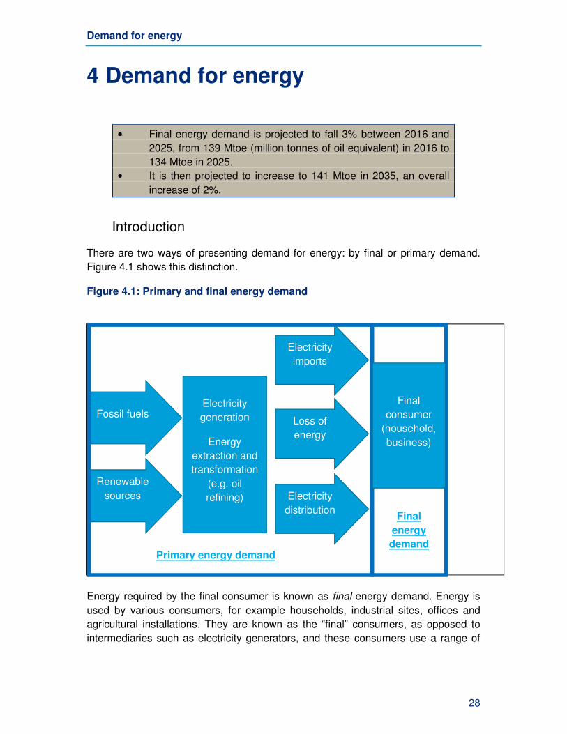
There are two ways of presenting demand for energy: by final or primary demand.
Figure 4.1 shows this distinction.
Figure 4.1: Primary and final energy demand
Energy required by the final consumer is known as final energy demand. Energy is
used by various consumers, for example households, industrial sites, offices and
agricultural installations. They are known as the “final” consumers, as opposed to
intermediaries such as electricity generators, and these consumers use a range of
Primary energy demand
Electricity
generation
Energy
extraction and
transformation
(e.g. oil
refining)
Fossil fuels
Renewable
sources
Final
energy
demand
Final
consumer
(household,
business)
Loss of
energy
Electricity
distribution
Electricity
imports
Demand for energy
29
different fuels. Electricity is usually generated off-site and distributed to consumers.
Fuels such as gas, biomass, oil and coal can also be burnt directly by the consumer.
Energy demand can also be described in terms of primary demand. In this case
electricity used by the final consumer is categorised by the fuel used to generate the
electricity. For example, fossil fuels, biomass or uranium used in power stations, or
the use of renewable energy such as from wind and solar. Primary energy demand
also includes loss of energy in the generation and distribution of electricity, net
imports of electricity from overseas, and energy used to extract and transform to
other energy forms e.g. in the oil refining industry.
Methodology for demand projections
For the Energy and Emissions Projections, final energy demand from 2017 to 2035
is projected by using statistical methods to estimate the historic relationship between
the underlying final energy consumption and key drivers of demand such as
economic growth, fuel prices and ambient temperature35. “Underlying consumption”
excludes the effect of policies which alter energy consumption36.
Specific relationships are estimated for demand for each fuel in each consumer
sector, e.g. electricity demand in the industrial sector. The projections of the demand
drivers are obtained from official sources37 and, together with the estimated
relationships, are used to produce projections of the underlying final energy demand.
A fundamental assumption of this approach is that the historic relationship is valid for
the duration of the projections.
To obtain projections of demand with the effect of policies included, the process
described in the last paragraph is “reversed”, i.e. an estimate of the change in future
energy consumption due to policies is subtracted from the projected underlying
energy demand.
In previous projections DUKES final energy demand statistics were adjusted to add
fuel used for heat sold to the demand figures for the sector buying the heat. This
adjustment was done using DUKES Annex J: Heat Sold Reallocation. Removing this
adjustment reduces 2016 final energy consumption by 1 Mtoe, mostly natural gas.
The change means that final fuel consumption statistics in the EEP are now aligned
with DUKES.
35
Data on historic (pre-2017) energy consumption is taken from the Digest of UK Energy Statistics (DUKES) 2017 edition: https://www.gov.uk/government/collections/digest-of-uk-energy-statistics-dukes 36
To remove the effect of policies, the change in historic energy consumption due to policies is modelled separately and then added to the actual final energy consumption. 37
See Annex M for details of the data sources for the drivers of demand.
Demand for energy
30
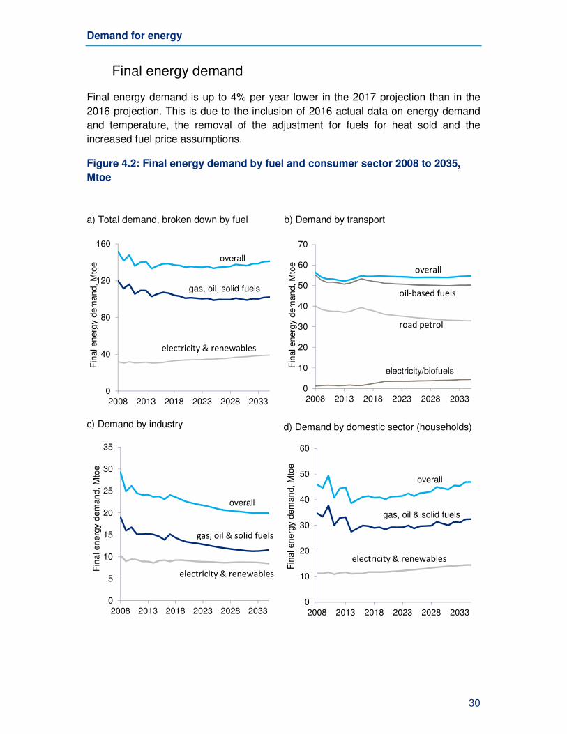
Final energy demand
Final energy demand is up to 4% per year lower in the 2017 projection than in the
2016 projection. This is due to the inclusion of 2016 actual data on energy demand
and temperature, the removal of the adjustment for fuels for heat sold and the
increased fuel price assumptions.
Figure 4.2: Final energy demand by fuel and consumer sector 2008 to 2035,
Mtoe
a) Total demand, broken down by fuel
b) Demand by transport
c) Demand by industry
d) Demand by domestic sector (households)
overall
0
40
80
120
160
2008 2013 2018 2023 2028 2033
Fin
al en
erg
y dem
and,
Mto
e
gas, oil, solid fuels
electricity & renewables
0
10
20
30
40
50
60
70
2008 2013 2018 2023 2028 2033
Fin
al energ
y dem
an
d, M
toe
electricity/biofuels
road petrol
oil-based fuels
overall
overall
0
5
10
15
20
25
30
35
2008 2013 2018 2023 2028 2033
Fin
al en
erg
y d
em
and,
Mto
e
electricity & renewables
gas, oil & solid fuels
overall
0
10
20
30
40
50
60
2008 2013 2018 2023 2028 2033
Fin
al energ
y dem
an
d, M
toe
gas, oil & solid fuels
electricity & renewables
31
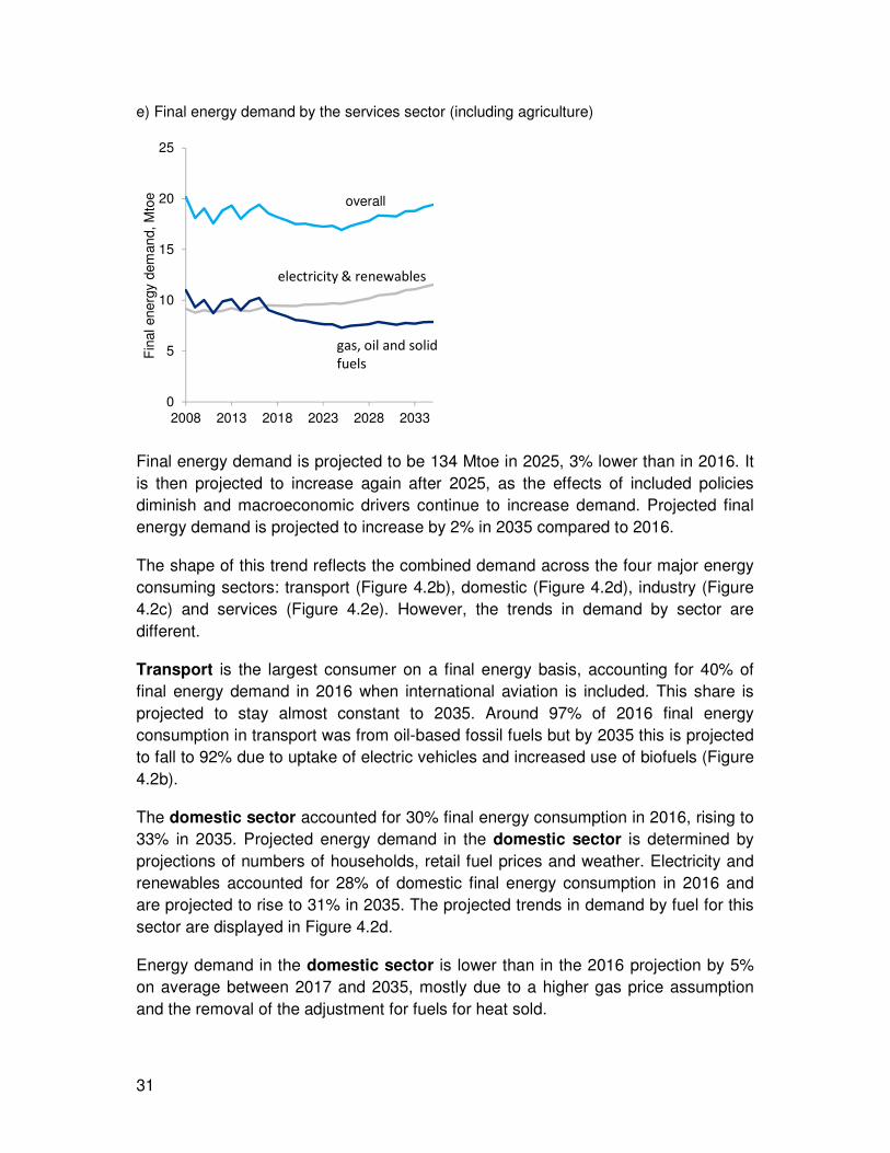
e) Final energy demand by the services sector (including agriculture)
Final energy demand is projected to be 134 Mtoe in 2025, 3% lower than in 2016. It
is then projected to increase again after 2025, as the effects of included policies
diminish and macroeconomic drivers continue to increase demand. Projected final
energy demand is projected to increase by 2% in 2035 compared to 2016.
The shape of this trend reflects the combined demand across the four major energy
consuming sectors: transport (Figure 4.2b), domestic (Figure 4.2d), industry (Figure
4.2c) and services (Figure 4.2e). However, the trends in demand by sector are
different.
Transport is the largest consumer on a final energy basis, accounting for 40% of
final energy demand in 2016 when international aviation is included. This share is
projected to stay almost constant to 2035. Around 97% of 2016 final energy
consumption in transport was from oil-based fossil fuels but by 2035 this is projected
to fall to 92% due to uptake of electric vehicles and increased use of biofuels (Figure
4.2b).
The domestic sector accounted for 30% final energy consumption in 2016, rising to
33% in 2035. Projected energy demand in the domestic sector is determined by
projections of numbers of households, retail fuel prices and weather. Electricity and
renewables accounted for 28% of domestic final energy consumption in 2016 and
are projected to rise to 31% in 2035. The projected trends in demand by fuel for this
sector are displayed in Figure 4.2d.
Energy demand in the domestic sector is lower than in the 2016 projection by 5%
on average between 2017 and 2035, mostly due to a higher gas price assumption
and the removal of the adjustment for fuels for heat sold.
overall
0
5
10
15
20
25
2008 2013 2018 2023 2028 2033
Fin
al energ
y dem
an
d, M
toe
gas, oil and solid
fuels
electricity & renewables
Demand for energy
32
The industrial sector accounted for 17% of total final energy in 2016. Demand is
projected to be around 6% per year lower than in the 2016 projections due to the
removal of the adjustment for fuels used for heat sold and higher fossil fuel prices.
In these projections, industrial energy demand is projected to fall by 13% overall
between 2016 and 2035. Renewables are projected to meet 10% of industrial energy
demand in 2030 compared to 6% in 2016. Projected trends in demand by fuels for
the industrial sector are displayed in Figure 4.2c.
The services sector accounted for 13% of final energy demand in 2016 and this
share remains almost constant through to 2035. The share of demand met by
electricity and renewables is projected to increase to 59% in 2035 from 47% in 2016
due to increasing electricity demand.
Final energy demand in the services sector in 2035 is 8% lower than in EEP 2016,
due to the update of winter degree days referred to in chapter 2 and higher fossil fuel
prices.
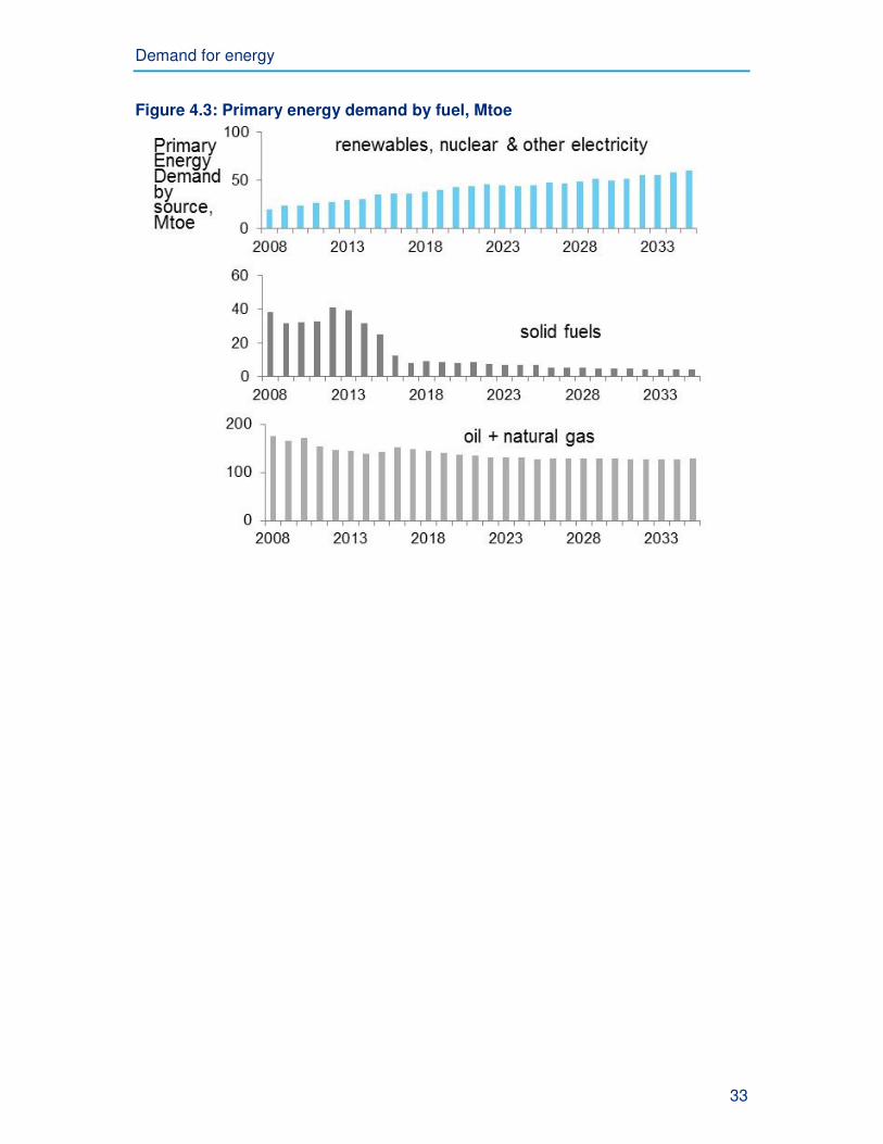
Primary energy demand
Trends in total primary energy demand are similar to EEP 2016, falling 11% between
2016 and 2025, from 201 to 179 Mtoe. After 2025, primary energy demand rises
again to 193 Mtoe in 2035.
Coal use has fallen rapidly since 2013 as electricity generation has switched to using
more renewables, waste and gas. By 2035, only 4 Mtoe of primary energy demand is
projected to be met by coal (from a total of 193 Mtoe). Oil use is projected to decline
by 8% in 2035 compared to 2016 levels as biofuels and electricity meet an
increasing proportion of road fuel demand.
In 2035 primary energy demand in the latest projection is 3% lower than in EEP
2016, but there are more significant changes in the mix of fuels meeting this
demand. Use of gas as a primary fuel is 17% lower in 2025 than in EEP 2016
because of the reduced final consumption of gas described previously and lower gas
consumption for electricity generation. However demand met by renewables and
waste is 26% higher in 2025 compared to EEP 2016. Use of nuclear fuel is reduced
in all years after 2025 compared to EEP 2016 (see chapter 5).
Demand for energy
33
Figure 4.3: Primary energy demand by fuel, Mtoe
Electricity supply
34
5 Electricity supply
• CO2 emissions from major power producers are projected to fall
by nearly 70% between 2010 and 2020.
• The low carbon share of UK electricity generation (renewables
and nuclear generation, as a proportion of all power producers)38
is projected to rise from 22% in 2010 to 58% in 2020.
• Beyond 2020, the scenario presented here is illustrative and
includes assumptions that may go beyond current Government
policy.
This section covers projections of electricity supply, the full results of which can be
found in Annexes G to L.
The electricity supply sector modelling was undertaken in September 2017 using
BEIS’s “Dynamic Dispatch Model” (DDM)39. The DDM models the impact of all
relevant policies including small scale Feed-in Tariffs, the Renewables Obligation,
Contracts for Difference, Carbon Price Support, the Capacity Market and Industrial
Emissions Directive.
Since EEP 2016, the DDM reference case assumptions have been updated with new
fossil fuel price assumptions, a revised carbon price floor trajectory and the latest
Contracts for Difference (CfD) auction results. There are also some changes to the
assumptions for future nuclear build40 (one less new plant by 2030) and Li-ion
battery storage capacity (slightly increased). Changes have also been made to the
electricity demand profiles of key electricity using technologies, and how this demand
may be shifted, and assumed system operability requirements.
In past EEP editions, all power station emissions were projected as traded under the
EUETS. This year, projections of emissions from ‘Energy from Waste’ power plants
are accounted for as ‘non-traded’.
38
Please note that statistics quoted in this chapter pertain to ‘All Power Producers’. In EEP 2016, most graphs were based on the less comprehensive category of ‘Major Power Producers’. 39
For detail on the DDM see: https://www.gov.uk/government/publications/dynamic-dispatch-model-ddm 40
These projections are not based on developers’ proposed pipeline of nuclear projects. Instead we have made a simplifying assumption of steady frequency of deployment of new nuclear plants. Whilst there are several projects in the pipeline, it would be improper for Government to pre-empt which of them will come forward and on what timelines.
Electricity supply
35
Up to 2020, the reference scenario reflects current power sector policies. Beyond
2020, the reference scenario includes some assumptions that go beyond current
Government policy, and is therefore illustrative. The results do not indicate a
preferred outcome and should also be treated as illustrative.
Results are presented separately for ‘Major Power Producers’ (MPPs) and ‘All Power
Producers’ (which includes ‘autogenerators’) in the report annexes. As of 2016,
MPPs accounted for around 95% of the UK’s electricity generation.
The definition of MPPs in EEP 2017 has been brought closer to the DUKES convention41. Thermal renewables based CHP plants are no longer counted as MPPs but as autogenerators, in accordance with DUKES convention42.
Summary of projections
Total electricity generation and generating capacity projections are very similar to
those in EEP 2016 and can be found in Annexes J and L of this report.
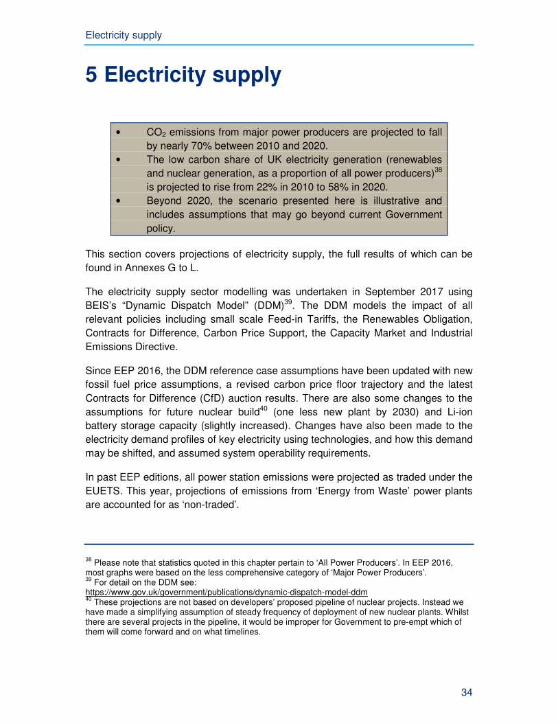
Figure 5.1, below, shows the projections of generation by technology for all power
producers to 2035. Source data can be found in Annex J.
Figure 5.1: Generation and net imports, TWh
41
The DUKES definition of MPPs is defined and discussed in paragraph 5.62 and following of DUKES 2017 https://www.gov.uk/government/uploads/system/uploads/attachment_data/file/643414/DUKES_2017.pdf 42
A remaining exception to the DUKES convention is a small number of CHP plants which are situated on MPP sites. These are still modelled and reported as MPP.
0
20
40
60
80
100
120
140
160
180
200
2017 2022 2027 2032
AllP
P g
en
era
tion b
y te
ch
nolo
gy
(TW
h)
Coal
Gas
Nuclear
Renewables
Net imports
Electricity supply
36
Following a sharp fall in coal fired generation in 2016, the DDM projects a further
gradual decline in fossil fuel based generation out to 2035. This is displaced by more
renewables and eventually nuclear based generation with increased imports (via
interconnectors) until new nuclear capacity reduces the need for this in the 2030s.
Emissions from electricity production are projected to fall steadily over the full period.
The vast majority of these emissions are covered by the EU Emissions Trading
System and therefore emissions savings have minimal direct impact on progress
towards meeting UK Carbon Budgets (see Box 1). However reducing power sector
emissions is important to meet our 2050 greenhouse gas emissions target.
In the reference case, CO2 emissions from electricity generation by major power
producers are projected to fall from 60 Mt in 2017 to 48 Mt by 2020. Under the
illustrative scenario presented for beyond 2020, emissions are projected to fall to 28
Mt in 2030. Further details of these projections can be seen in annexes B and C.
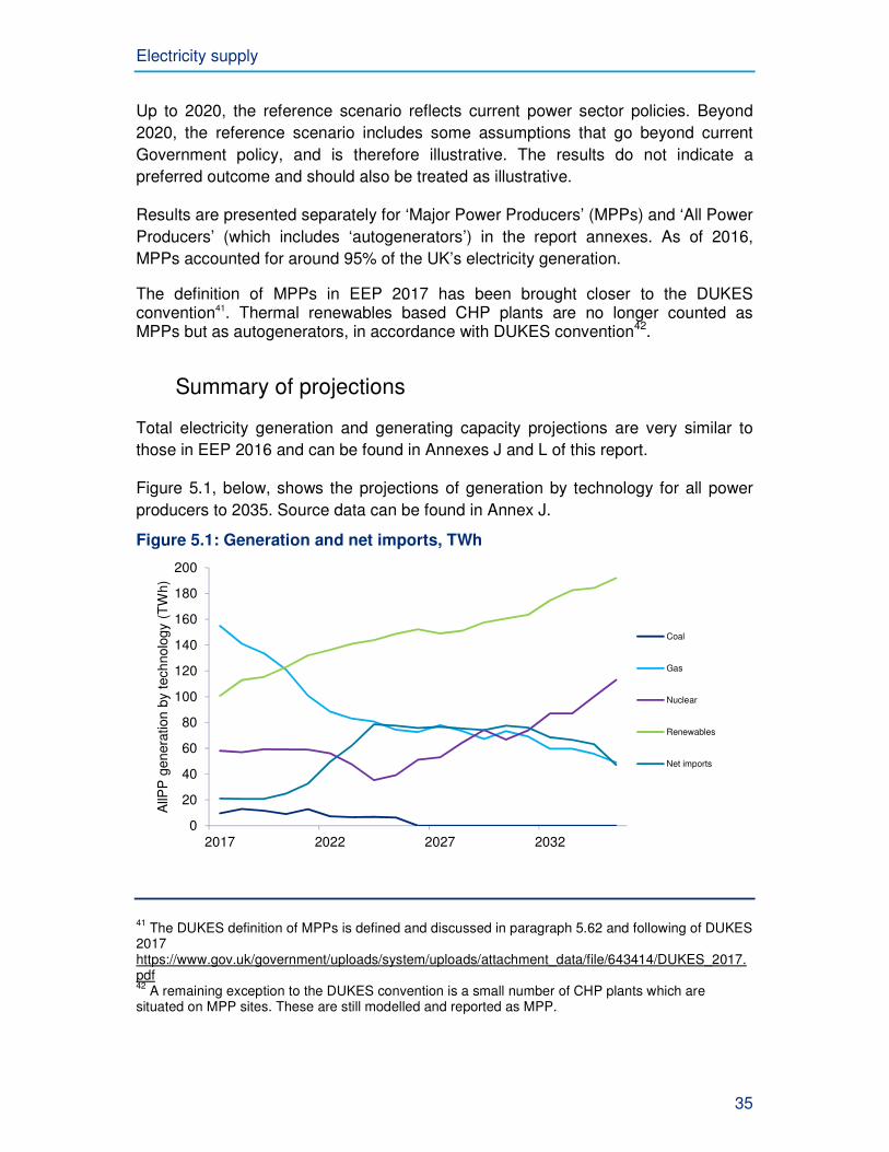
Figure 5.2: Emissions intensity (vs EEP 2016), gCO2e/kWh43
Figure 5.2 shows a lower trajectory of power sector emissions intensity between
2017 and 2030 in EEP 2017 (in comparison to EEP 2016). This is predominantly
because some coal generation is replaced by gas in the projections up to 2020 whilst
there is less curtailment of wind generation after 2020, compared to EEP 2016. As
shown above, the projected emissions intensity in 2030 (104 gCO2e/kWh) is similar
to that in EEP 2016 (107 gCO2e/kWh).
43
Figure 5.2 includes both CO2 and non-CO2 greenhouse gases
0
50
100
150
200
250
300
2017 2022 2027 2032
Em
issio
ns in
ten
sity,
gC
O2e
/KW
h
EEP 2017
EEP 2016
Electricity supply
37
Revised system operability requirements from National Grid allow greater
penetration of renewables in this year’s EEP44.
Autogenerators
Autogenerators are electricity plants owned by businesses whose main activity is not
electricity generation. They are mostly comprised of ‘Good Quality’ CHP (Combined
Heat and Power) schemes that have been certified by the UK’s CHP Quality
Assurance (CHPQA) programme. There is also some CHP capacity which does not
qualify as ‘Good Quality’ under the CHPQA programme, as well as a small amount
of pure autogeneration (with no exported heat). The latter is projected independently
and is estimated to comprise less than 0.5 GW total capacity in all years.
For EEP 2017, the DDM (BEIS’s model for electricity supply modelling) has been
improved to incorporate all Combined Heat and Power (CHP) plants amongst its
modelling of the wider electricity market. Previously most CHP had been modelled
separately.
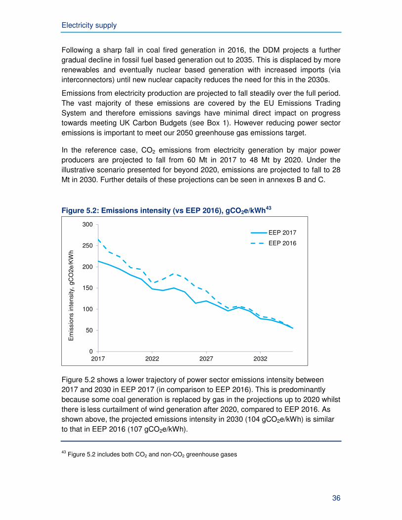
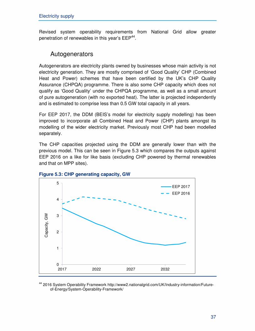
The CHP capacities projected using the DDM are generally lower than with the
previous model. This can be seen in Figure 5.3 which compares the outputs against
EEP 2016 on a like for like basis (excluding CHP powered by thermal renewables
and that on MPP sites).
Figure 5.3: CHP generating capacity, GW
44
2016 System Operability Framework http://www2.nationalgrid.com/UK/Industry-information/Future-of-Energy/System-Operability-Framework/
0
1
2
3
4
5
2017 2022 2027 2032
Capacity,
GW
EEP 2017
EEP 2016
Electricity supply
38
EEP 2017 projections show a gradual decline in CHP capacity until the early 2030s,
continuing the declining trend of Good Quality CHP since 2010, observed in DUKES
historical data. The change in the projections since EEP 2016 is purely a result of the
different modelling methodology this year and is not due to any change in
Government policy.
Uncertainty in emissions projections
39
6 Uncertainty in emissions projections
• Uncertainty analysis for 2017 considers more variables than
EEP 2016, and additionally includes analysis of uncertainty
within model equations and of structural breaks.
• Within this chapter, we report uncertainty based on four
categories: policy savings, evidence base inputs, state of the
world (which includes factors such as GDP, population and fossil
fuel prices) and model equations.
• By the fourth carbon budget period, the greatest uncertainty
comes from the state of the world category (approximately +/-
5%). Evidence base showed +/- 2% variability, while policies and
industry equation uncertainty both showed about 1.5% for this
carbon budget period.
Since EEP 2016, BEIS has improved the approach used to estimate the uncertainty
of the Energy and Emissions Projections. This chapter sets out different sources of
uncertainty and the extent to which they are reflected in these projections. As with
last year, it should be noted that uncertainty analysis excludes the electricity supply
industry, and so does not capture uncertainty on the effects of policies in this sector.
It is helpful to understand the significant scale of uncertainty, the scope for the future
to turn out differently and what influences this. This is important context in our efforts
to reduce emissions, highlighting the value of a flexible and responsive approach.
Different sources of uncertainty
As with any other projections, our energy and emissions projections are subject to a degree of uncertainty. This uncertainty comes from different sources: there are four broad steps to producing our projections, and each has uncertainty surround it.
Step 1 – estimate historic drivers of energy use: Using historic data, we estimate
the relationships between key drivers and energy use. For example, we estimate the
historic impact of fossil fuel prices, population and GDP on energy use.
Uncertainty: we cannot be certain of the relationships between drivers of
energy use and emissions because of limits in available historical data and
because we cannot assess all possible drivers. For the 2017 projections, we
Uncertainty in emissions projections
40
have partly captured this uncertainty by estimating the error in the model
equations in the industry sector.
Step 2 – forecast key drivers which shape the ‘state of the world’: We use
forecasts of key drivers as a starting point for the projections (alongside the current
energy mix). For example, we use projections of future coal, oil and gas prices, and
of future population and GDP growth.
Uncertainty: For many of the drivers it is not possible to forecast with high
accuracy, particularly over periods of more than 15 years. We have captured
some of this uncertainty in our projections analysis by testing a range of
different forecasts for the most influential key drivers. These are summarised
in Table 6.1.
Step 3 – apply historic relationships to forecast of key drivers: We assume that
the historic relationship between key drivers and energy use (estimated in step 1) will
continue into the future.
Uncertainty: we assume that estimated historic relationships will continue
unchanged in the future, however relationships could change. Historic trends
may break down, for example, with structural breaks such as high-impact
innovations or changes in behaviour. In summer 2017, we undertook a pilot
project to identify possible structural break scenarios with a significant
impact on the energy sector and to estimate their impact. The work has not
been included in the main uncertainty analysis, but is discussed later in this
chapter.
Step 4 – estimate impact of policies on energy use: Steps 1-3 produce the
baseline projections scenario. We then adjust this with estimates of recent policy
impacts on energy use. For example, we estimate the recent fuel savings from
efficiency policies and switching between fuels driven by clean energy policies.
Uncertainty: we cannot be sure of the exact impact our policies will have,
and so we also estimate a range of uncertainty around our central
projections of policy impacts. These uncertainty ranges are reflected in this
report (see Table 6.1). Uncertainty analysis excludes the electricity supply
industry, and so does not capture uncertainty on the effects of policies in this
sector.
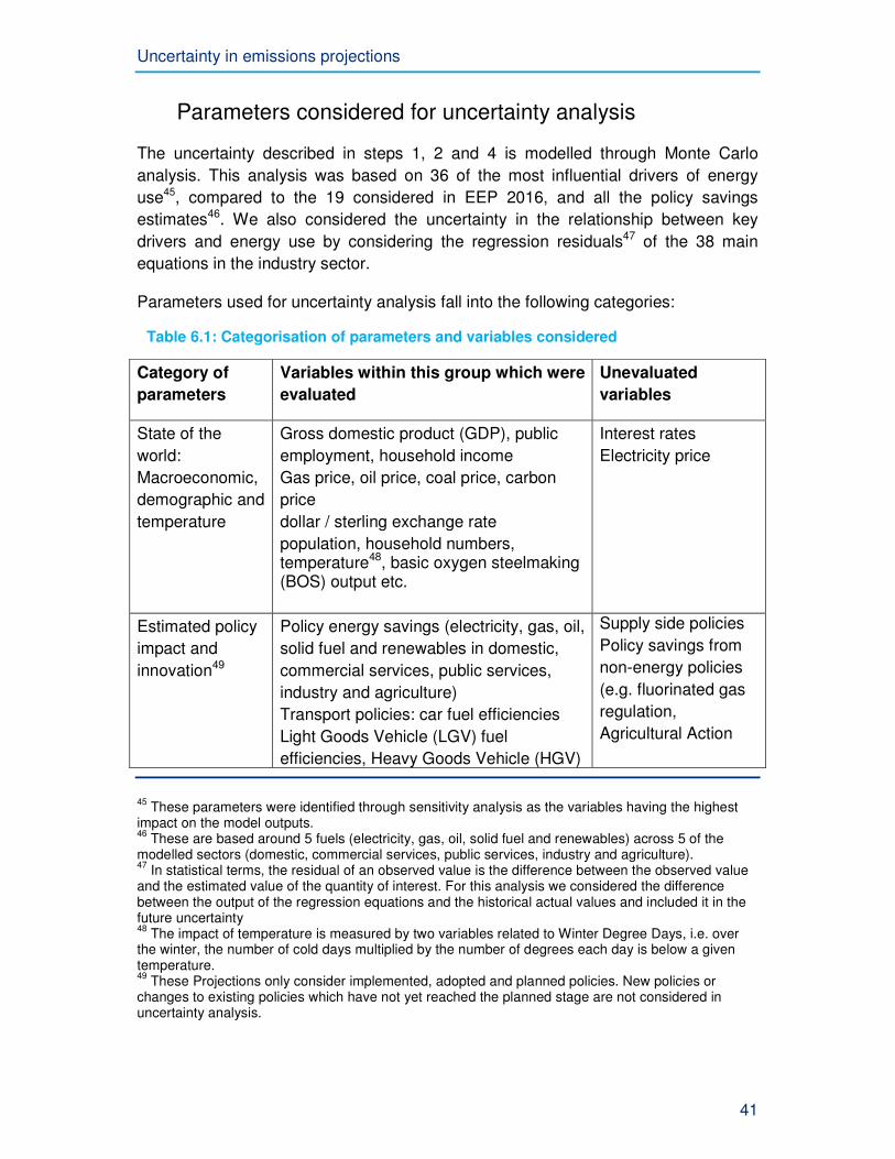
Uncertainty in emissions projections
41
Parameters considered for uncertainty analysis
The uncertainty described in steps 1, 2 and 4 is modelled through Monte Carlo
analysis. This analysis was based on 36 of the most influential drivers of energy
use45, compared to the 19 considered in EEP 2016, and all the policy savings
estimates46. We also considered the uncertainty in the relationship between key
drivers and energy use by considering the regression residuals47 of the 38 main
equations in the industry sector.
Parameters used for uncertainty analysis fall into the following categories:
Table 6.1: Categorisation of parameters and variables considered
Category of
parameters
Variables within this group which were
evaluated
Unevaluated
variables
State of the
world:
Macroeconomic,
demographic and
temperature
Gross domestic product (GDP), public
employment, household income
Gas price, oil price, coal price, carbon
price
dollar / sterling exchange rate
population, household numbers, temperature48, basic oxygen steelmaking (BOS) output etc.
Interest rates
Electricity price
Estimated policy
impact and
innovation49
Policy energy savings (electricity, gas, oil,
solid fuel and renewables in domestic,
commercial services, public services,
industry and agriculture)
Transport policies: car fuel efficiencies
Light Goods Vehicle (LGV) fuel
efficiencies, Heavy Goods Vehicle (HGV)
Supply side policies
Policy savings from
non-energy policies
(e.g. fluorinated gas
regulation,
Agricultural Action
45
These parameters were identified through sensitivity analysis as the variables having the highest impact on the model outputs. 46
These are based around 5 fuels (electricity, gas, oil, solid fuel and renewables) across 5 of the modelled sectors (domestic, commercial services, public services, industry and agriculture). 47
In statistical terms, the residual of an observed value is the difference between the observed value and the estimated value of the quantity of interest. For this analysis we considered the difference between the output of the regression equations and the historical actual values and included it in the future uncertainty 48
The impact of temperature is measured by two variables related to Winter Degree Days, i.e. over the winter, the number of cold days multiplied by the number of degrees each day is below a given temperature. 49
These Projections only consider implemented, adopted and planned policies. New policies or changes to existing policies which have not yet reached the planned stage are not considered in uncertainty analysis.
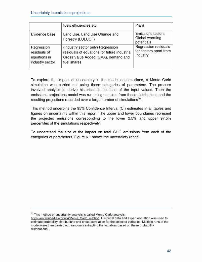
Uncertainty in emissions projections
42
fuels efficiencies etc. Plan)
Evidence base Land Use, Land Use Change and
Forestry (LULUCF)
Emissions factors Global warming potentials
Regression
residuals of
equations in
industry sector
(Industry sector only) Regression
residuals of equations for future industrial
Gross Value Added (GVA), demand and
fuel shares
Regression residuals for sectors apart from Industry
To explore the impact of uncertainty in the model on emissions, a Monte Carlo
simulation was carried out using these categories of parameters. The process
involved analysis to derive historical distributions of the input values. Then the
emissions projections model was run using samples from these distributions and the
resulting projections recorded over a large number of simulations50.
This method underpins the 95% Confidence Interval (CI) estimates in all tables and
figures on uncertainty within this report. The upper and lower boundaries represent
the projected emissions corresponding to the lower 2.5% and upper 97.5%
percentiles of the simulations respectively.
To understand the size of the impact on total GHG emissions from each of the
categories of parameters, Figure 6.1 shows the uncertainty range.
50
This method of uncertainty analysis is called Monte Carlo analysis: https://en.wikipedia.org/wiki/Monte_Carlo_method. Historical data and expert elicitation was used to estimate probability distributions and cross-correlation for the selected variables. Multiple runs of the model were then carried out, randomly extracting the variables based on these probability distributions.
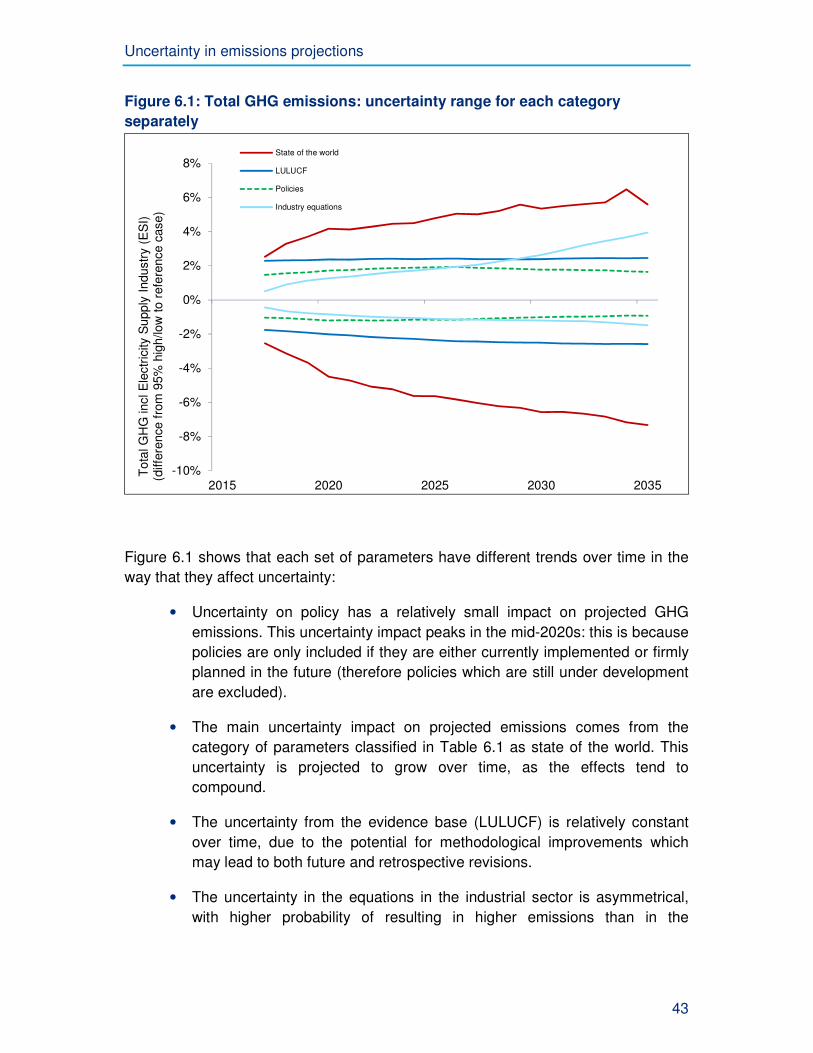
Uncertainty in emissions projections
43
Figure 6.1: Total GHG emissions: uncertainty range for each category
separately
Figure 6.1 shows that each set of parameters have different trends over time in the
way that they affect uncertainty:
• Uncertainty on policy has a relatively small impact on projected GHG
emissions. This uncertainty impact peaks in the mid-2020s: this is because
policies are only included if they are either currently implemented or firmly
planned in the future (therefore policies which are still under development
are excluded).
• The main uncertainty impact on projected emissions comes from the
category of parameters classified in Table 6.1 as state of the world. This
uncertainty is projected to grow over time, as the effects tend to
compound.
• The uncertainty from the evidence base (LULUCF) is relatively constant
over time, due to the potential for methodological improvements which
may lead to both future and retrospective revisions.
• The uncertainty in the equations in the industrial sector is asymmetrical,
with higher probability of resulting in higher emissions than in the
-10%
-8%
-6%
-4%
-2%
0%
2%
4%
6%
8%
2015 2020 2025 2030 2035
To
tal G
HG
incl E
lectr
icity
Su
pply
Industr
y (E
SI)
(d
iffe
rence
fro
m 9
5%
hig
h/low
to
refe
rence c
ase)
State of the world
LULUCF
Policies
Industry equations
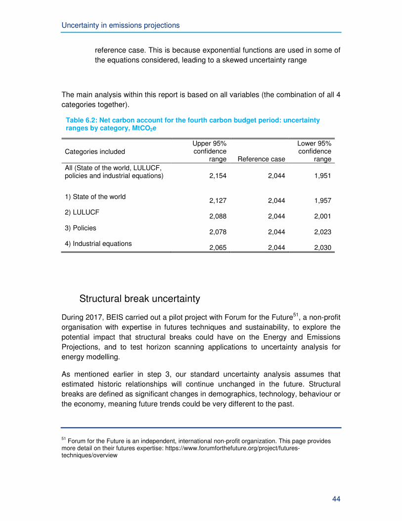
Uncertainty in emissions projections
44
reference case. This is because exponential functions are used in some of
the equations considered, leading to a skewed uncertainty range
The main analysis within this report is based on all variables (the combination of all 4
categories together).
Table 6.2: Net carbon account for the fourth carbon budget period: uncertainty ranges by category, MtCO2e
Categories included
Upper 95% confidence
range Reference case
Lower 95% confidence
range
All (State of the world, LULUCF, policies and industrial equations)
2,154
2,044
1,951
1) State of the world
2,127
2,044
1,957
2) LULUCF
2,088
2,044
2,001
3) Policies
2,078
2,044
2,023
4) Industrial equations
2,065
2,044
2,030
Structural break uncertainty
During 2017, BEIS carried out a pilot project with Forum for the Future51, a non-profit
organisation with expertise in futures techniques and sustainability, to explore the
potential impact that structural breaks could have on the Energy and Emissions
Projections, and to test horizon scanning applications to uncertainty analysis for
energy modelling.
As mentioned earlier in step 3, our standard uncertainty analysis assumes that
estimated historic relationships will continue unchanged in the future. Structural
breaks are defined as significant changes in demographics, technology, behaviour or
the economy, meaning future trends could be very different to the past.
51
Forum for the Future is an independent, international non-profit organization. This page provides more detail on their futures expertise: https://www.forumforthefuture.org/project/futures-techniques/overview
Uncertainty in emissions projections
45
This analysis focused on externally driven changes which are not primarily led by
Government policy52, but would still have a significant impact on energy use and
greenhouse gas emissions and the success of policies relating to energy and climate
change.
To do this, BEIS selected a subset of key variables used for modelling these
Projections, including energy demand for households, services, and various
industrial sectors. Forum for the Future then researched potential structural breaks
which could widen the uncertainty range already considered for these variables.
Forum for the Future created two exploratory scenarios based on their existing
collection of scenarios (and the research and interviews that informed those), and
further desk research and conversations. This gave an indication of how quickly and
how significantly the scenarios might impact on emissions.
1. Scenario A explored changes which would primarily affect buildings and housing,
and could lead to a sharp reduction in emissions compared to the EEP
reference case. The scenario considered structural breaks related to
technological innovation in new materials and societal preferences for low-
carbon buildings and infrastructure. In this scenario, innovation in business
models could enhance the appeal of retrofitting, and smart grid/internet of
things could help informed consumers to reduce energy used in existing
buildings.
2. Scenario B explored changes in manufacturing, where emerging digital trends in
automation, 3D printing and robotics could combine with societal trends for
localisation and personalisation, leading to increased UK manufacturing. This
could lead to an increase in UK GDP and higher emissions compared to the
reference case, as production and transport emissions would shift to the UK.
Additionally, small-scale production and local transportation could be more
carbon-intensive than mass production.
As this work was only a pilot, the challenge was in identifying the scale of change
plausible. Given this, results need to be treated as ‘informed guesstimates’ so
graphs are not presented here. However this analysis showed that this approach has
strong potential in helping to identify additional factors for uncertainty analysis, and
we hope to continue this further in future editions of the Energy and Emissions
Projections.
52
For the central scenario of this analysis we considered the status of the world as projected in the EEP reference case, which includes only implemented, adopted and planned policies.
Uncertainty in emissions projections
46
Uncertainties not covered in this analysis
The results presented in this chapter are likely to be an underestimate of the actual
uncertainty in the projections. The main sources of residual uncertainty are:
• The analysis assumed that all policy inputs varied independently;
• For EEP 2017, we added a new category of uncertainty (regression residuals
for the industry sector), however we do not yet include this analysis for other
sectors;
• As in previous years, uncertainty analysis excludes the electricity supply
industry. This is because it is currently not possible to run the electricity
supply model with all combinations of the different inputs. Therefore this
analysis does not capture uncertainty on the effects of policies in the
electricity supply sector;
• Given the very high number of variables used in the model, it was not possible
to consider all of them in the Monte Carlo simulation. However, we increased
the number of variables considered (compared to EEP 2016) and we ranked
all variables in order of their impact on the outputs and included those
estimated to be most influential on emissions;
• The distributions and correlations used in the Monte Carlo simulation are
approximations, sometimes based on limited historical data that often require
a level of subjectivity to interpret;
• The methodology used assumes that the future variability in the key
parameters will be similar to the historical variability. This approach is not able
to take into account the possibility of structural changes in the system, which
may arise due to innovation or changes in behaviour. The pilot project we
described in the section above is an attempt to reduce the impact of this
modelling limitation and we are planning to do more work on this next year;
• The methodology focuses on future uncertainty, rather than analysis of how
uncertain inputs or outputs may have been historically, i.e. before 2017.
Conclusions
Understanding the scale and sources of uncertainty is important context for
interpreting these projections.
It is clear that as we look further into the future, uncertainty grows. Whilst the
analysis above can give us these insights, it is far from exhaustive and we know
there are other sources of uncertainty not fully captured. Further work is underway to
better understand the scope for innovation and changing societal behaviours to
reshape future energy and emissions. These insights underline the value of flexibility
and responsiveness in policy design, particularly in areas with a long-term outlook,
such as the transition to a low carbon economy.
Lists of supporting material
47
7 Lists of supporting material
Annexes
Annex A: Greenhouse gas emissions by source
Annex B: Carbon dioxide emissions by source
Annex C: Carbon dioxide emissions by IPCC category
Annex D: Policy savings in the projections
Annex E: Primary energy demand
Annex F: Final energy demand
Annex G: Major power producers’ generation by source
Annex H: Major power producers’ cumulative new electricity generating
capacity
Annex I: Major power producers’ total electricity generating capacity
Annex J: Total electricity generation by source
Annex K: Total cumulative new electricity generating capacity
Annex L: Total electricity generating capacity
Annex M: Growth assumptions and prices
Annex N: 2017 non-CO2 GHG emissions projections report
Web tables and charts
Web tables and charts have been uploaded alongside this report. Some of these replicate
tables and figures within this report, others are supplementary.
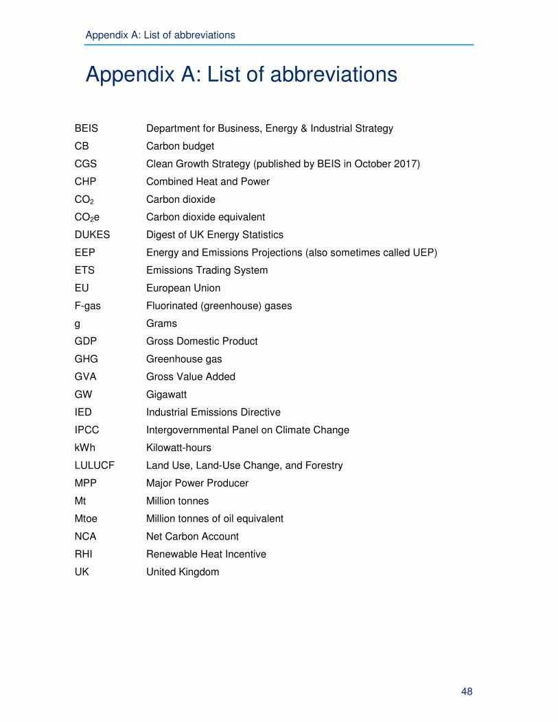
Appendix A: List of abbreviations
48
Appendix A: List of abbreviations
BEIS Department for Business, Energy & Industrial Strategy
CB Carbon budget
CGS Clean Growth Strategy (published by BEIS in October 2017)
CHP Combined Heat and Power
CO2 Carbon dioxide
CO2e Carbon dioxide equivalent
DUKES Digest of UK Energy Statistics
EEP Energy and Emissions Projections (also sometimes called UEP)
ETS Emissions Trading System
EU European Union
F-gas Fluorinated (greenhouse) gases
g Grams
GDP Gross Domestic Product
GHG Greenhouse gas
GVA Gross Value Added
GW Gigawatt
IED Industrial Emissions Directive
IPCC Intergovernmental Panel on Climate Change
kWh Kilowatt-hours
LULUCF Land Use, Land-Use Change, and Forestry
MPP Major Power Producer
Mt Million tonnes
Mtoe Million tonnes of oil equivalent
NCA Net Carbon Account
RHI Renewable Heat Incentive
UK United Kingdom