Urban growth simulation using V-BUDEM

1School of Urban Planning and Design, Peking University2Nijmegen School of Management, Radboud University Nijmegen3School of City and Regional Planning, Cardiff University4Beijing Institute of City Planning

Yongping ZHANG1,2,3, Ying LONG4*

2013-08

a vector-based Beijing urban development model

Outline

• 1. Introduction• 2. V-BUDEM• 3. Model application• 4. Conclusion and discussion

1. INTRODUCTION

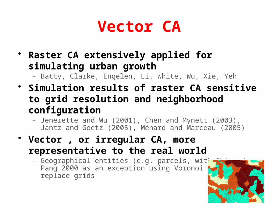
• Raster CA extensively applied for simulating urban growth– Batty, Clarke, Engelen, Li, White, Wu, Xie, Yeh

• Simulation results of raster CA sensitive to grid resolution and neighborhood configuration– Jenerette and Wu (2001), Chen and Mynett (2003), Jantz and Goetz

(2005), Ménard and Marceau (2005)

• Vector , or irregular CA, more representative to the real world– Geographical entities (e.g. parcels, with Shi and Pang 2000 as an

exception using Voronoi polygon) replace grids

Vector CA

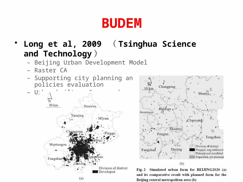
• Long et al, 2009 （ Tsinghua Science and Technology）– Beijing Urban Development Model– Raster CA– Supporting city planning and corresponding policies evaluation – Urban built-up & non urban built-up

BUDEM

• Improve initial raster BUDEM into vector V-BUDEM

• Focused on the urban growth simulation at this stage

• Test it in a small town of Beijing

This paper is regarded with

2. V-BUDEM

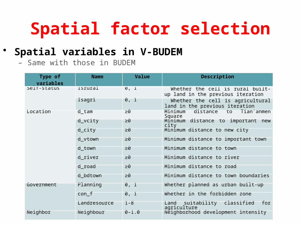
• Spatial variables in V-BUDEM – Same with those in BUDEM

Spatial factor selection

Type of variables Name Value Description

Self-status Isrural 0, 1 Whether the cell is rural built-up land in the previous iteration

Isagri 0, 1 Whether the cell is agricultural land in the previous iteration

Location 

d_tam ≥0 Minimum distance to Tian’anmen Square

d_vcity ≥0 Minimum distance to important new city

d_city ≥0 Minimum distance to new city

d_vtown ≥0 Minimum distance to important town

d_town ≥0 Minimum distance to town

d_river ≥0 Minimum distance to river

d_road ≥0 Minimum distance to road

d_bdtown ≥0 Minimum distance to town boundaries

Government Planning 0, 1 Whether planned as urban built-up

con_f 0, 1 Whether in the forbidden zone

Landresource 1-8 Land suitability classified for agriculture

Neighbor Neighbour 0-1.0 Neighborhood development intensity

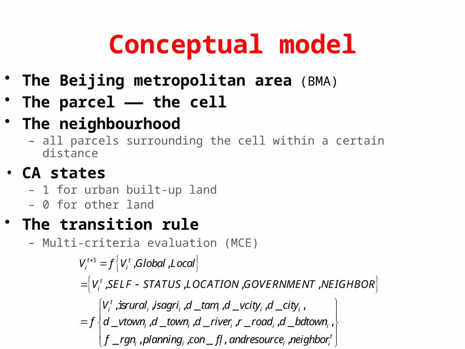
• The Beijing metropolitan area (BMA)

• The parcel —— the cell• The neighbourhood

– all parcels surrounding the cell within a certain distance

• CA states – 1 for urban built-up land– 0 for other land

• The transition rule– Multi-criteria evaluation (MCE)

Conceptual model

1 , ,

, , , ,

, is , , _ , _ , _ ,

_ , _ , _ , _ , _ ,

_ , , _ , ,

t ti i

ti

ti i i i i i

i i i i i

i i i i

V f V Global Local

V SELF STATUS LOCATION GOVERNMENT NEIGHBOR

V rural isagri d tam d vcity d city

f d vtown d town d river r road d bdtown

f rgn planning con f landresource nei

tighbor

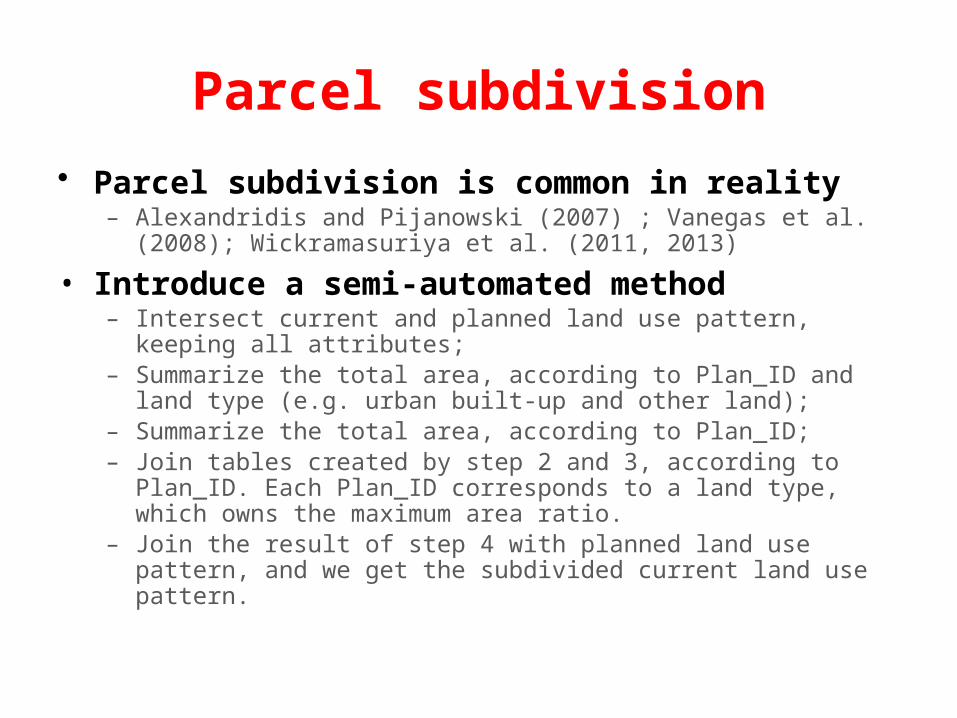
• Parcel subdivision is common in reality– Alexandridis and Pijanowski (2007) ; Vanegas et al. (2008);

Wickramasuriya et al. (2011, 2013)

• Introduce a semi-automated method – Intersect current and planned land use pattern, keeping all attributes;– Summarize the total area, according to Plan_ID and land type (e.g.

urban built-up and other land);– Summarize the total area, according to Plan_ID;– Join tables created by step 2 and 3, according to Plan_ID. Each

Plan_ID corresponds to a land type, which owns the maximum area ratio.

– Join the result of step 4 with planned land use pattern, and we get the subdivided current land use pattern.

Parcel subdivision

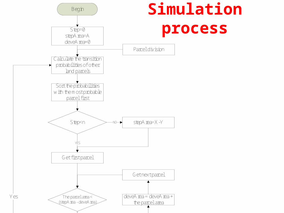
Simulation processBegin

Calculate the transition probabilities of other

land parcels

End

Sort the probabilities with the most probable

parcel first

Get first parcel

The parcel area < (stepArea - deveArea)

The parcel developed

deveArea = deveArea + the parcel area

YES

YES

Iteration finished

Yes

Update other land parcels

NO

Step = Step + 1

Step=0stepArea=A deveArea=0

Step<n

YES

NO

Get next parcel

stepArea=X-YStep<n NO

Parcel division

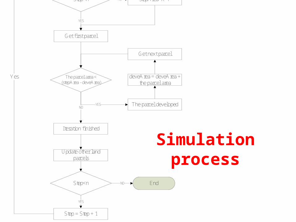
Simulation process

Begin

Calculate the transition probabilities of other

land parcels

End

Sort the probabilities with the most probable

parcel first

Get first parcel

The parcel area < (stepArea - deveArea)

The parcel developed

deveArea = deveArea + the parcel area

YES

YES

Iteration finished

Yes

Update other land parcels

NO

Step = Step + 1

Step=0stepArea=A deveArea=0

Step<n

YES

NO

Get next parcel

stepArea=X-YStep<n NO

Parcel division

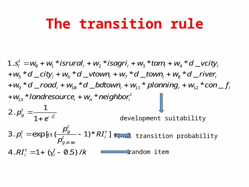
The transition rule

0 1 2 3 4

5 6 7 8

9 10 11 12

13

1. * * * * _

* _ * _ * _ * _

* _ * _ * * _

* *

12.

1

3. e

ti

ti i i i i

i i i i

i i i i

ti n i

tg s

ti

s w w isrural w isagri w tam w d vcity

w d city w d vtown w d town w d river

w d road w d bdtown w planning w con f

w landresource w neighbor

pe

p

,max

xp[ ( 1)* ]

4. 1 ( 0.5) /

tg t

itg

t ti i

pRI

p

RI k

development suitability

final transition probability

random item

3. MODEL APPLICATION

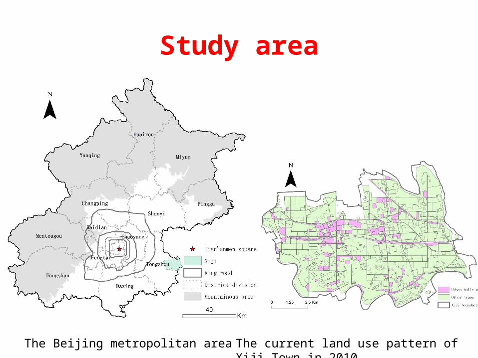
Study area

The Beijing metropolitan area The current land use pattern of Xiji Town in 2010

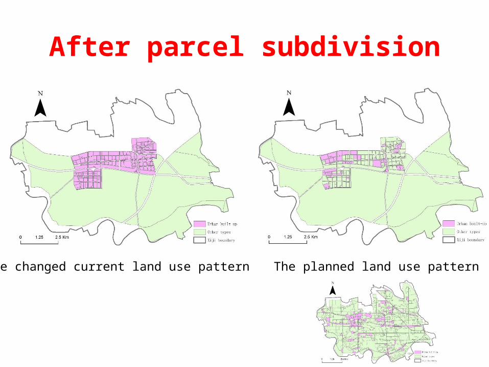
After parcel subdivision

The changed current land use pattern The planned land use pattern

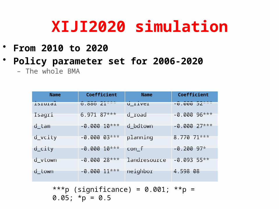
• From 2010 to 2020• Policy parameter set for 2006-2020

– The whole BMA

XIJI2020 simulation

Name Coefficient Name Coefficient

isrural 6.886 21*** d_river -0.000 52***

Isagri 6.971 87*** d_road -0.000 96***

d_tam -0.000 10*** d_bdtown -0.000 27***

d_vcity -0.000 03*** planning 8.770 71***

d_city -0.000 10*** con_f -0.200 97*

d_vtown -0.000 28*** landresource -0.093 55**

d_town -0.000 11*** neighbor 4.598 08

***p (significance) = 0.001; **p = 0.05; *p = 0.5

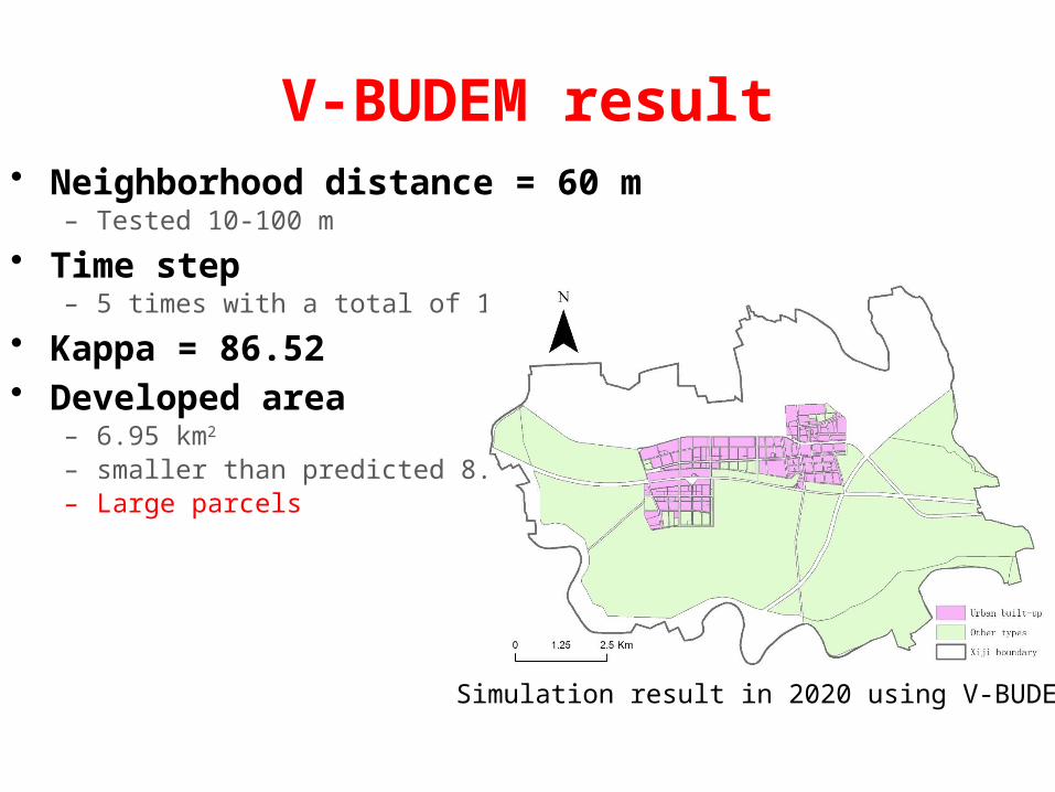
• Neighborhood distance = 60 m – Tested 10-100 m

• Time step – 5 times with a total of 10 years

• Kappa = 86.52• Developed area

– 6.95 km2

– smaller than predicted 8.77 km2

– Large parcels

V-BUDEM result

Simulation result in 2020 using V-BUDEM

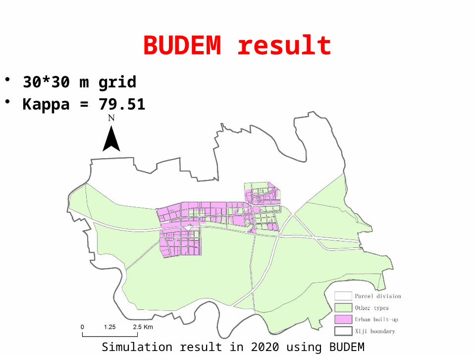
• 30*30 m grid• Kappa = 79.51

BUDEM result

Simulation result in 2020 using BUDEM

• Using the parameter set to Xiji in V-BUDEM was comparatively more suitable than that in BUDEM

• In V-BUDEM– The parcel would be developed or undeveloped as a whole unit

• In BUDEM– Part areas of some parcels would be transited into urban built-up land,

while other part areas would keep other land type• Unlikely to be happened in reality

– Parcel space was a little different with the space consisted by grid• For cell boundary could be out of parcel boundary, and it could cause some

inaccuracies as a result.

Result comparison

5. CONCLUSION AND DISCUSSION

• V-BUDEM was proposed, and a preliminary test was conducted– more close to the real situation

• aiming to the application of urban planning– comprehensive constraints– basic farmland protection and forbidden built-up areas

• The semi-automated parcel subdivision method– a new solution– determine the basic simulation spatial units for V-BUDEM– easy to implement and speed-up the model run

Conclusion

• Expand to the whole BMA• Integrated automated parcel subdivision tool

– Wickramasuriya et al. (2011)

• Established the land use pattern in detail– Residential, commercial, and industrial land types– Planner Agent (Zhang and Long, 2013)

Future work

Thanks！longying1980@gmail.com