AD

TECHNICAL REPORT ARCCB-TR-98013

DYNAMIC MODELING FOR DESIGN: SPACE-TIME FINITE ELEMENT

FORMULATION OF AN EULER BEAM

ERIC L. KÄTHE

JULY 1998

US ARMY ARMAMENT RESEARCH, DEVELOPMENT AND ENGINEERING CENTER

CLOSE COMBAT ARMAMENTS CENTER BENET LABORATORIES

WATERVLIET, N.Y. 12189-4050

APPROVED FOR PUBLIC RELEASE; DISTRIBUTION UNLIMITED

Sflö QCAUTy INSPECTED I

DISCLAIM»

The findings In this report are not to bo construed is an official

Department of tho Any position «loss so designated by othor authorised

documents,

Tho uso of trado name(s) and/or manufacturer(s) dot« not constitute

an official indorscasnt or approval.

OESTTOCTXON Nona

For classified documents, follow tho procodurts in DoO 5200.22-M,

Industrial Security Manual, Section XZ-19 or DoD S200.1-R, Information

Security Protran Regulation, Chapter IX.

For unclassified, limittd docuaents, destroy by any method that will

prevent disclosure of contents or reconstruction of tht document.

For unclassified, unlimited documents, destroy when the report is

no longer needed. Do not return it to the originator.

REPORT DOCUMENTATION PAGE Form Approved

OMB No. 0704-0188

Public repo'tnc Pu"d?n for tnis coi-ert.er. of o:orrr.atiC- is estimated '.o a.erage ' hour per response including the tims for reviewing iost',;cti:,r,r searrhi gather i no and maintaining the data needeo and completing anc review-.r-z the collection of information Seno comments reaaraing this burger, es'.irr.?tr cr

collection of informs:,: r.. including suqcesiions fcr recu:lrg tr-.is burcen to '/.ashmgcon Headauarte's Servir.es, Directorate for information One^a tiers anc Da-, is Hichwa,, Sj'tc- '2C- Arlington. 71". 22202-J3C2 and to the Office of Management and Budget. Paperwork Reduction Project (07CJ-Q'86i. Vvash.ngoon.

: e>- st,ng data sources in, otne' aspect of th-s ■erx-'.s, 1215 Jefferson

1. AGENCY USE ONLY (Leave blank) 2. REPORT DATS July 1998

-L.

3. REPORT TYPE AND DATES COVERED

Final

6. TITLE AND SUBTITLE

DYNAMIC MODELING FOR DESIGN: SPACE-TIME FINITE ELEMENT FORMULATION OF AN EULER BEAM

6. AUTHOR(S)

Eric L. Kathe

5. FUNDING NUMBERS

AMCMS No. 6226.24.H 180.0 PRON No. 4A7A7FYA1ABJ

7. PERFORMING ORGANIZATION NAME(S) AND ADDRESS(ES)

U.S. Army ARDEC Benet Laboratories, AMSTA-AR-CCB-0 Watervliet, NY 12189-4050

8. PERFORMING ORGANIZATION REPORT NUMBER

ARCCB-TR-98013

S. SPONSORING/MONITORING AGENCY NAMEiS; AND ADDRESS(ES)

U.S. Army ARDEC Close Combat Armaments Center Picatinny Arsenal, NJ 07806-5000

10. SPONSORING/MONITOR!:.; AGENCY RFPORT NUVl..

11. SUPPLEMENTARY NOT Presented at the 68"' Shock and Vibration Symposium, Baltimore, MD, 3-7 November 1997. Published in Proceedings of the Symposium.

12c. DISTRIBUTION AVAILABILITY STATEMEK"!

Approved for public release; distribution unlimited.

12b. DISTRIBUTION cor-:

IS. AE-LTF./■■■■:'! i/v,i>/>-,■ i./t.;'a;. ■.'.■-X.;:

This paper demonstrates the application of finite element methods in both space and time to the partial differential equations that govern beam dynamics. The approach enables design problems for the structural response of beams subject to shock and vibration loading to be posed. Numerical validation of the results using a forward Euler ordinary differential equation solver is also shown.

U. SUEUECY TERN. Structural Dynamics, Space-Time Finite Element Analysis, Optimal Design

"ib NUMBER OF PAGE:

20

17. SECURITY UASSiflCMIü OF REPCF.

{UNCLASSIHED NSN 75AO-0'.-28C-5-;0-J

U SECURITY CLASSIFICATION 1S. SECURITY CLASSIFICATION: OF TKIS FAG; OF ABSTRACT

UNCLASSIFIED UNCLASSIFIED

1£. PRICE COD-

20. LIMITATION OF ABSTRAC

Standard Form 298 '.Re, 2-89;

TECHNICAL REPORT ARCCB-TR-98013

DYNAMIC MODELING FOR DESIGN: SPACE-TIME FINITE ELEMENT

FORMULATION OF AN EULER BEAM

ERIC L. KÄTHE

JULY 1998

July 1998 Final

DYNAMIC MODELING FOR DESIGN: SPACE-TIME FINITE ELEMENT FORMULATION OF AN EULER BEAM

AMCMS No. 6226.24.H 180.0 PRONNo. 4A7A7FYA1ABJ

.:»

Eric L. Kathe

U.S. Army ARDEC Benet Laboratories. AMSTA-AR-CCB-0 Watcrvlict, NY 12189-4050

ARCCB-TR-98013

U.S. Army ARDEC Close Combat Armaments Center Picatinny Arsenal. NJ 07806-5000

Presented at the 68"' Shock and Vibration Symposium, Baltimore. MD, 3-7 November 1997. Published in Proceedings of the Symposium.

Approved for public release; distribution unlimited.

This paper demonstrates the application of Unite element methods in both space and time to the partial differential equations that govern beam' dynamics. The approach enables design problems for the structural response of beams subject to shock and vibration loading to be posed. Numerical validation of the results using a forward Euler ordinary differential equation solver is also shown. .- -

Structural Dynamics, Space-Time Finite Element Analysis, Optimal Design 20

UNCLASSIFIED UNCLASSIFIED UNCLASSIFIED UL

TABLE OF CONTENTS Page

ACKNOWLEDGMENTS iii

PREFACE iv

INTRODUCTION 1

THE SPATIAL FINITE ELEMENT MODEL 1

VARIATIONAL STATEMENT OF THE PROBLEM 2

TEMPORAL FINITE ELEMENT FORMULATION 3

Definition of a Finite Element Basis 3

Finite Element Formulation of the Variational Statement 4

Extrication of the Coefficient Matrix from the Variational Integration 4

INCLUSION OF INITIAL CONDITIONS 6

NUMERICAL VALIDATION OF THE RESULTS 8

DESIGN OPTIMIZATION 10

Segregation of a Design Parameter 10

Taylor Series Approximation 10

Weighted Quadratic Objective Function 11

CASE STUDY: DESIGN OF A VIBRATION ABSORBER CONSTRAINT 12

The Design Objective 12

Taylor Series Convergence 12

Objective Function Definition 12

CONCLUSIONS 14

Final Notes 15

REFERENCES 16

LIST OF ILLUSTRATIONS

1. Homogeneous response of the beam to an isolated initial velocity of the beam with a magnitude of 0.05 (lateral displacement time), just forward of the cantilevered root at y, 9

2. Forced response of the same beam shown in Figure 1 with a vibration absorber coupled at the tip to an impulsive force applied to the beam, just forward of the cantilevered root at y, 9

3. Taylor series convergence contour plot 13

4. Plot of the objective function, J(Ace) 13

5. Forced response of the same beam of Figure 2 with the optimal absorber stiffness identified in Figure 4 13

6. Several design cases to achieve a desired zero crossing 14

ACKNOWLEDGMENTS

The author would like to acknowledge the assistance of Drs. Michael Coyle and Ronald Racicot, Benet Labs, and Professors Joeseph Flaherty and Andrew Lemnios, Rensselaer Polytechnic Institute, Troy, NY.

in

PREFACE

In the late 1970s and the early 1980s, gun dynamics research and engineering at Ben6t Laboratories began to focus on finite elements in space and time—with a desire to reduce the demands placed on the computational hardware platforms of the day.

However, finite elements in time are inherently problematic. The distinction between the forward motion of an object in time and heat or stress distribution on an object in space is not subtle. Causality—the property of real dynamic systems that says that future inputs cannot affect current response—is not provided any particular safeguard, and the straightforward application of variation principles does not appear to work. (At least, this author's attempts thus far have failed.) Thus, Simkins employed an unorthodox approach using Lagrange multipliers, which included boundary condition terms that normally drop out of the formulation, while Wu examined the adjoint operator and avoided the unknown boundary conditions by setting a "stiffness" to a numeric equivalent of infinity. (See Wu, J. J. and Simkins, T. E., "A Numerical Comparison Between Two Unconstrained Variational Formulations," ARLCB-TR-79024, September 1979.)

This challenge aside, this author contends that structural dynamic problems, posed in their entirety in both space and time, provide a uniquely powerful holistic perspective from which to view the design optimization process—regardless of the variational approach used to formulate the temporal dynamics. This perspective or vantage point closes the gap between numerical experiment (simulation) and modeling for design. This paper presents a simplified design problem—which was posed using finite elements in space and time—that demonstrates the potential utility of space-time finite element modeling as a new design tool. It is hoped that this will encourage feedback from the research, engineering, and development communities regarding space-time finite element modeling.

Although not trivial, inclusion of the state-dependent loading that defines the moving mass problem (gun dynamics) has been demonstrated in the past; thus, the design method presented here may be extended to launch dynamics of most large caliber weapon systems. In addition, the nature of the design method and the availability of an analytic Jacobian lends itself to optimization in high dimensional design spaces, where the potential utility versus simulation are clear.

Thus, with the emphasis placed on optimization in a high dimension parametric space, the next obvious question is: "What is there to design? A gun is merely a glorified tapered cylindrical pressure vessel." This author contends that a gun is a structural conduit that imparts a great deal of kinetic energy to a projectile, and subsequently accumulates both kinetic and strain energy within itself during launch. Designing the structure to accumulate as little energy as possible or to divert the energy to the least sensitive portions of the structure is critical to the future effectiveness of precision cannons. This area of inquiry is wide open for exploitation using non-traditional structural modification. Thus, maturation of a new design method may shed light on the bottom of Pandora's box prior to opening it.

iv

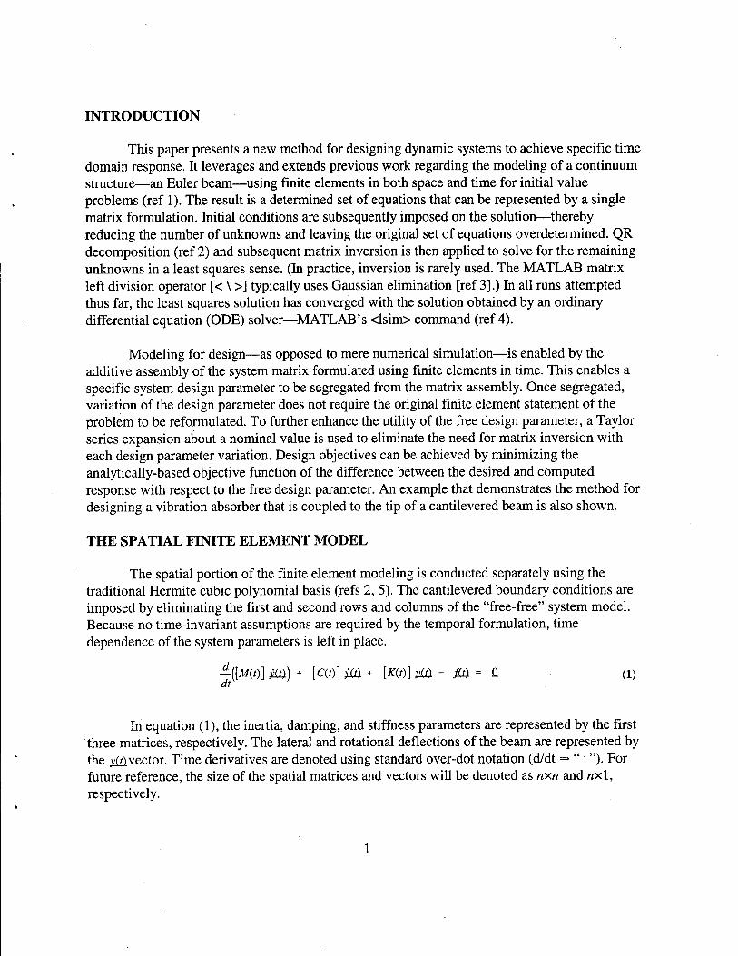
INTRODUCTION

This paper presents a new method for designing dynamic systems to achieve specific time domain response. It leverages and extends previous work regarding the modeling of a continuum structure—an Euler beam—using finite elements in both space and time for initial value problems (ref 1). The result is a determined set of equations that can be represented by a single matrix formulation. Initial conditions are subsequently imposed on the solution—thereby reducing the number of unknowns and leaving the original set of equations overdetermined. QR decomposition (ref 2) and subsequent matrix inversion is then applied to solve for the remaining unknowns in a least squares sense. (In practice, inversion is rarely used. The MATLAB matrix left division operator [< \ >] typically uses Gaussian elimination [ref 3].) In all runs attempted thus far, the least squares solution has converged with the solution obtained by an ordinary differential equation (ODE) solver—MATLAB's <lsim> command (ref 4).

Modeling for design—as opposed to mere numerical simulation—is enabled by the additive assembly of the system matrix formulated using finite elements in time. This enables a specific system design parameter to be segregated from the matrix assembly. Once segregated, variation of the design parameter does not require the original finite element statement of the problem to be reformulated. To further enhance the utility of the free design parameter, a Taylor series expansion about a nominal value is used to eliminate the need for matrix inversion with each design parameter variation. Design objectives can be achieved by minimizing the analytically-based objective function of the difference between the desired and computed response with respect to the free design parameter. An example that demonstrates the method for designing a vibration absorber that is coupled to the tip of a cantilevered beam is also shown.

THE SPATIAL FINITE ELEMENT MODEL

The spatial portion of the finite element modeling is conducted separately using the traditional Hermite cubic polynomial basis (refs 2, 5). The cantilevered boundary conditions are imposed by eliminating the first and second rows and columns of the "free-free" system model. Because no time-invariant assumptions are required by the temporal formulation, time dependence of the system parameters is left in place.

-([M(O] m)+ [c(o] m + [KW] m - m = Q (D dt

In equation (1), the inertia, damping, and stiffness parameters are represented by the first three matrices, respectively. The lateral and rotational deflections of the beam are represented by the yitxvector. Time derivatives are denoted using standard over-dot notation (d/dt =» " "). For future reference, the size of the spatial matrices and vectors will be denoted as nxn and nxl, respectively.

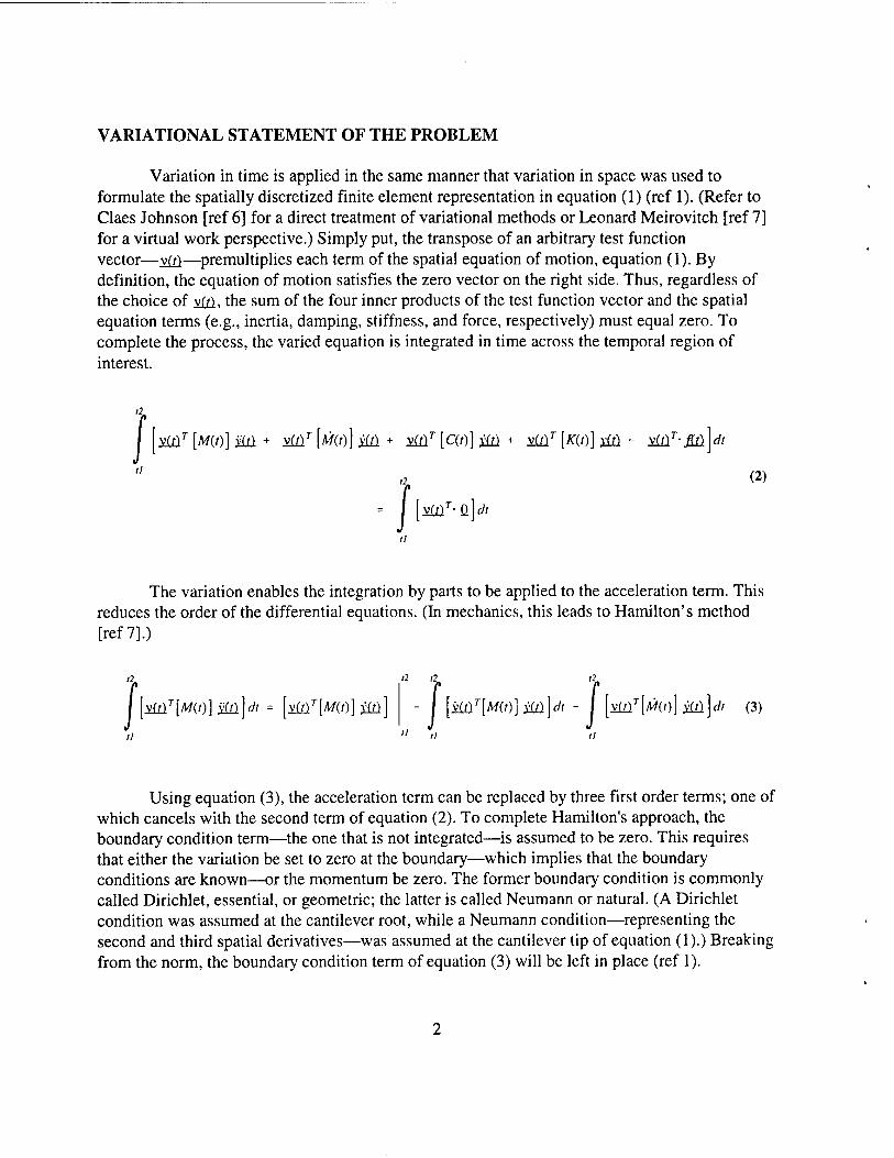
VARIATIONAL STATEMENT OF THE PROBLEM

Variation in time is applied in the same manner that variation in space was used to formulate the spatially discretized finite element representation in equation (1) (ref 1). (Refer to Claes Johnson [ref 6] for a direct treatment of variational methods or Leonard Meirovitch [ref 7] for a virtual work perspective.) Simply put, the transpose of an arbitrary test function vector—v£/)—premultiplies each term of the spatial equation of motion, equation (1). By definition, the equation of motion satisfies the zero vector on the right side. Thus, regardless of the choice of v£f}, the sum of the four inner products of the test function vector and the spatial equation terms (e.g., inertia, damping, stiffness, and force, respectively) must equal zero. To complete the process, the varied equation is integrated in time across the temporal region of interest.

vmr [Mio] m+ xinT k(o] m + üMr [c(o] m + rf [*(o] m - mT-m dt

I [v£Ür'ü]^

(2)

The variation enables the integration by parts to be applied to the acceleration term. This reduces the order of the differential equations. (In mechanics, this leads to Hamilton's method [ref 7].)

1 mT[M(t)}m\dt = \mT[M{t)]m

12 12

I [mT[mt)]m]dt - I [vMr[M(o]im]^ @)

Using equation (3), the acceleration term can be replaced by three first order terms; one of which cancels with the second term of equation (2). To complete Hamilton's approach, the boundary condition term—the one that is not integrated—is assumed to be zero. This requires that either the variation be set to zero at the boundary—which implies that the boundary conditions are known—or the momentum be zero. The former boundary condition is commonly called Dirichlet, essential, or geometric; the latter is called Neumann or natural. (A Dirichlet condition was assumed at the cantilever root, while a Neumann condition—representing the second and third spatial derivatives—was assumed at the cantilever tip of equation (1).) Breaking from the norm, the boundary condition term of equation (3) will be left in place (ref 1).

TEMPORAL FINITE ELEMENT FORMULATION

Definition of a Finite Element Basis

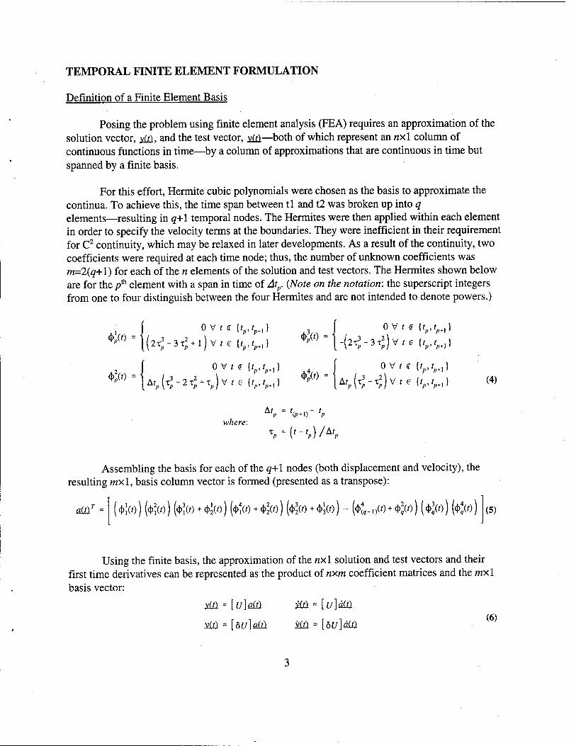
Posing the problem using finite element analysis (FEA) requires an approximation of the solution vector, yj&, and the test vector, v£ü—both of which represent an nxl column of continuous functions in time—by a column of approximations that are continuous in time but spanned by a finite basis.

For this effort, Hermite cubic polynomials were chosen as the basis to approximate the continua. To achieve this, the time span between tl and t2 was broken up into q elements—resulting in q+1 temporal nodes. The Hermites were then applied within each element in order to specify the velocity terms at the boundaries. They were inefficient in their requirement for C2 continuity, which may be relaxed in later developments. As a result of the continuity, two coefficients were required at each time node; thus, the number of unknown coefficients was m=2(q+l) for each of the n elements of the solution and test vectors. The Hermites shown below are for the pth element with a span in time of Atp. {Note on the notation: the superscript integers from one to four distinguish between the four Hermites and are not intended to denote powers.)

.2 J ov/fivv.) .4,, I ovr* {fp,fp+1} *>® = JA^-2x^)v,e {r,.r,+ll ^ = j Ar, ft -,]) V , e „,.,,„ } (4)

AtP= '(p..)" <P

where: T

P=(f-fp)/A'/>

Assembling the basis for each of the q+l nodes (both displacement and velocity), the resulting mxl, basis column vector is formed (presented as a transpose):

dixT = d>ko) (tfw) (d>?(o + *J(o) (*t(o + *2(o) (*2« + <l>fr)) ••• (<C,(o + <#o) (*;«) (<(o) (5)

Using the finite basis, the approximation of the nxl solution and test vectors and their first time derivatives can be represented as the product of nxm coefficient matrices and the mxl basis vector:

m*[u]m ma[u]m

via = [5[/]fl(ä m - [bu]m (6)

Equation (6) clarifies that the coefficient matrices bear no burden with re: pect to the time derivative. Their coefficients are not a function of time; only the basis is a function of time. Also, use of the 8 notation—which is common to virtual work—distinguishes between the solution and the test function coefficients. (As a simplified example, if n = 1, this implies that equation (1) represents a one degree of freedom system, [U] and its variation [öU] would be \xm vector transposes.)

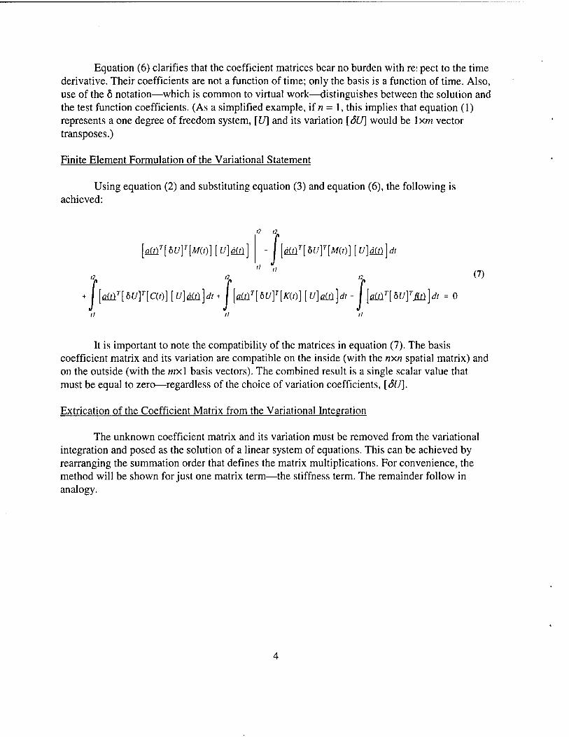
Finite Element Formulation of the Variational Statement

Using equation (2) and substituting equation (3) and equation (6), the following is achieved:

a a

amT[bU]T[M(t)][u]m \mT[?>u}T[M(t)}[u]<m\dt

J'2n ,2n ^

lmT[?>u]T[c(t)][u}m]dt +1 [aw.T[^uY[K(t)][u]m}dt-1 [mT[?>u]Tm}dt = o

// ti a

It is important to note the compatibility of the matrices in equation (7). The basis coefficient matrix and its variation are compatible on the inside (with the nxn spatial matrix) and on the outside (with the mxl basis vectors). The combined result is a single scalar value that must be equal to zero—regardless of the choice of variation coefficients, [SU].

Extrication of the Coefficient Matrix from the Variational Integration

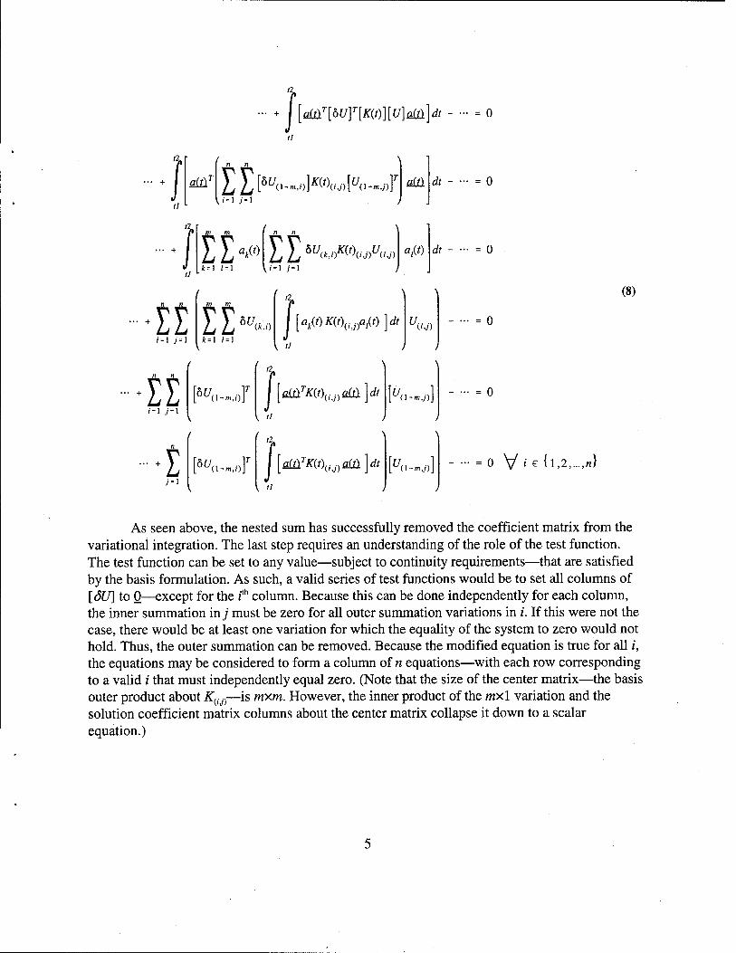
The unknown coefficient matrix and its variation must be removed from the variational integration and posed as the solution of a linear system of equations. This can be achieved by rearranging the summation order that defines the matrix multiplications. For convenience, the method will be shown for just one matrix term—the stiffness term. The remainder follow in analogy.

I [mT[w] '[m][u]m\dt

fl n n

mT ££K~m,o]*«,,;,[t/(1,mJ)f

fm m In n_ t2.

8WW)

flOEl

a,(0

*

A

1=1 ;=i

n n

EE n

E j=i

^(.-.oir

K-m,olr

n n m m i*

11 EE6y- J[

fl

\ak(t)K(t\.jff.t) \dt

V "

I/, (/J)

flca^w^flüip V ti

u, (1-")J)

m'K(%,nm\dt U, (l-mj)

= 0

= 0

= 0

= 0

(8)

= 0 V ' e {l,2,...,«}

As seen above, the nested sum has successfully removed the coefficient matrix from the variational integration. The last step requires an understanding of the role of the test function. The test function can be set to any value—subject to continuity requirements—that are satisfied by the basis formulation. As such, a valid series of test functions would be to set all columns of [ÖU] to 0—except for the z-th column. Because this can be done independently for each column, the inner summation in j must be zero for all outer summation variations in i. If this were not the case, there would be at least one variation for which the equality of the system to zero would not hold. Thus, the outer summation can be removed. Because the modified equation is true for all i, the equations may be considered to form a column of n equations—with each row corresponding to a valid i that must independently equal zero. (Note that the size of the center matrix—the basis outer product about K(ij)—is mxm. However, the inner product of the mxl variation and the solution coefficient matrix columns about the center matrix collapse it down to a scalar equation.)

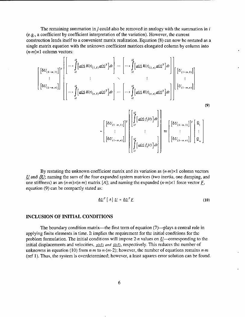
The remaining summation in j could also be removed in analogy with the summation in i (e.g., a coefficient by coefficient interpretation of the variation). However, the current construction lends itself to a convenient matrix realization. Equation (8) can now be restated as a single matrix equation with the unknown coefficient matrices elongated column by column into (n-m)xl column vectors:

bu, (l-m,l)

w (l-m,n)

a a j[aitiK(t)0l)amT}dt +f[mK(t\Un)QmT]dt

a ■ + f[a!ümln-y)m

T]dt

hV. <l-m,l)

St/, (l-m,n)

a

- + \[QlilK(t\nn)eitiT)di

u, (1-m,1)

U, (l-m,n)

(9)

|[fl£U/,(0]*

(2

/[ flM/„(0 rfr

6f7, (l-m.l)

61/, (l-m.n) Ü

By restating the unknown coefficient matrix and its variation as (n-m)xl column vectors U and ÖU; naming the sum of the four expanded system matrices (two inertia, one damping, and one stiffness) as an (n-m)x(n-m) matrix [A]; and naming the expanded (nm)x\ force vector F, equation (9) can be compactly stated as:

M1T[A] LI = MlTE (10)

INCLUSION OF INITIAL CONDITIONS

The boundary condition matrix—the first term of equation (7)—plays a central role in applying finite elements in time. It implies the requirement for the initial conditions for the problem formulation. The initial conditions will impose 1-n values on U—corresponding to the initial displacements and velocities, y(tJ) and y(tl). respectively. This reduces the number of unknowns in equation (10) from n-m to n-(m-2); however, the number of equations remains n-m (ref 1). Thus, the system is overdetermined; however, a least squares error solution can be found.

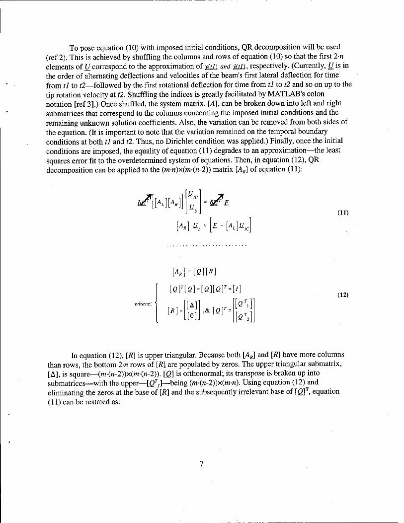
To pose equation (10) with imposed initial conditions, QR decomposition will be used (ref 2). This is achieved by shuffling the columns and rows of equation (10) so that the first 2-n elements of U correspond to the approximation of yiül and yitiy, respectively. (Currently, U is in the order of alternating deflections and velocities of the beam's first lateral deflection for time from tl to t2—followed by the first rotational deflection for time from tl to t2 and so on up to the tip rotation velocity at t2. Shuffling the indices is greatly facilitated by MATLAB's colon notation [ref 3].) Once shuffled, the system matrix, [A], can be broken down into left and right submatrices that correspond to the columns concerning the imposed initial conditions and the remaining unknown solution coefficients. Also, the variation can be removed from both sides of the equation. (It is important to note that the variation remained on the temporal boundary conditions at both tl and tl. Thus, no Dirichlet condition was applied.) Finally, once the initial conditions are imposed, the equality of equation (11) degrades to an approximation—the least squares error fit to the overdetermined system of equations. Then, in equation (12), QR decomposition can be applied to the (m-n)x(m-(n-2)) matrix [AR] of equation (11):

S^[K]K UK

LL^ (ID

:om [QYlQh [Q][QY* M

where: '

[*] = [A]'

.&[ß]r =

(12)

In equation (12), [R] is upper triangular. Because both [AR] and [R] have more columns than rows, the bottom 2-n rows of [R] are populated by zeros. The upper triangular submatrix, [A], is square—(m-(n-2))x(m-(n-2)). [Q] is orthonormal; its transpose is broken up into submatrices—with the upper— [(?,]—being (m-(n-2))x(wn). Using equation (12) and eliminating the zeros at the base of [R] and the subsequently irrelevant base of [ß]T, equation (11) can be restated as:

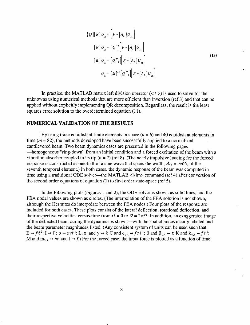
\Q}[R]llb*\E-[AL]lL

[R]llb*[Q]T[E-[AL]lL

[A]iZ^[ßM[£-K]i//c

Ub~~[AV[Q\}\E-[AL]Uic

(13)

In practice, the MATLAB matrix left division operator (< \ >) is used to solve for the unknowns using numerical methods that are more efficient than inversion (ref 3) and that can be applied without explicitly implementing QR decomposition. Regardless, the result is the least squares error solution to the overdetermined equation (11).

NUMERICAL VALIDATION OF THE RESULTS

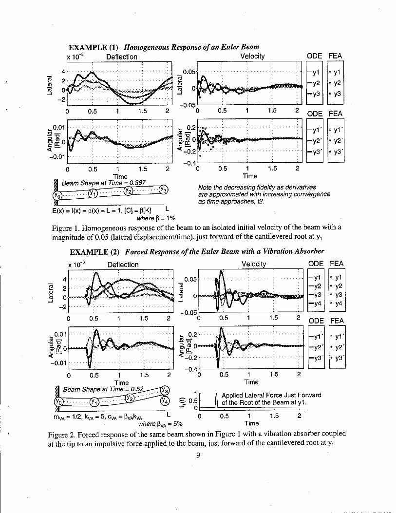
By using three equidistant finite elements in space (n = 6) and 40 equidistant elements in time (m = 82), the methods developed have been successfully applied to a normalized, cantilevered beam. Two beam dynamics cases are presented in the following pages —homogeneous "ring-down" from an initial condition and a forced excitation of the beam with a vibration absorber coupled to its tip (n = 7) (ref 8). (The nearly impulsive loading for the forced response is constructed as one-half of a sine wave that spans the width, At7 = TI/60, of the seventh temporal element.) In both cases, the dynamic response of the beam was computed in time using a traditional ODE solver—the MATLAB <lsim> command (ref 4) after conversion of the second order equations of equation (1) to first order state-space (ref 5).

In the following plots (Figures 1 and 2), the ODE solver is shown as solid lines, and the FEA nodal values are shown as circles. (The interpolation of the FEA solution is not shown, although the Hermites do interpolate between the FEA nodes.) Four plots of the response are included for both cases. These plots consist of the lateral deflection, rotational deflection, and their respective velocities versus time from tl = 0 to t2 = 2TT/3. In addition, an exaggerated image of the deflected beam during the dynamics is shown—with the spatial nodes clearly labeled and the beam parameter magnitudes listed. (Any consistent system of units can be used such that: E =*/-f2; I => V4; p - m-rl; L, x, and y => {; C and cVA =»/-H''; ß and ßVA - t\ K and kVA =>/-f'; M and mVA =» m; and f:

*VA

VA J ' * ' K ""u KVA '' "■ "11U 'n'A /.) For the forced case, the input force is plotted as a function of time.

EXAMPLE (1) Homogeneous Response of an Euler Beam x10~ Deflection Velocity

•

0.5 1.5

0

Beam

1 Time

■ at Time = 0.367

ODE FEA

-y1 o y-|

-y2 . y2

-y3 • y3

ODE FEA

-y1' o yl'

-y2' . y2'

-y3' • y3'

Note the decreasing fidelity as derivatives are approximated with increasing convergence as time approaches, t2.

E(x) = l(x) = p(x) = L = 1,[C] = ß[K] L where$ = \%

Figure 1. Homogeneous response of the beam to an isolated initial velocity of the beam with a magnitude of 0.05 (lateral displacement/time), just forward of the cantilevered root at yj

EXAMPLE (2) Forced Response of the Euler Beam with a Vibration Absorber

x10" Deflection Velocity

03

0) to

ODE FEA

-y1 o y1

-y2 o y2

-y3 • y3 -y4 o y4

FEA ODE

-y1' o y-|'

-y2' • y2'

-y3' • y3'

1 Time

1.5

Applied Lateral Force Just Forward of the Root of the Beam at y1.

1 Time

1.5 mVA = 1/2, kVA = 5, cVA = ßvAkvA where ßVA = 5%

Figure 2. Forced response of the same beam shown in Figure 1 with a vibration absorber coupled at the tip to an impulsive force applied to the beam, just forward of the cantilevered root at y{

9

DESIGN OPTIMIZATION

Segregation of a Design Parameter

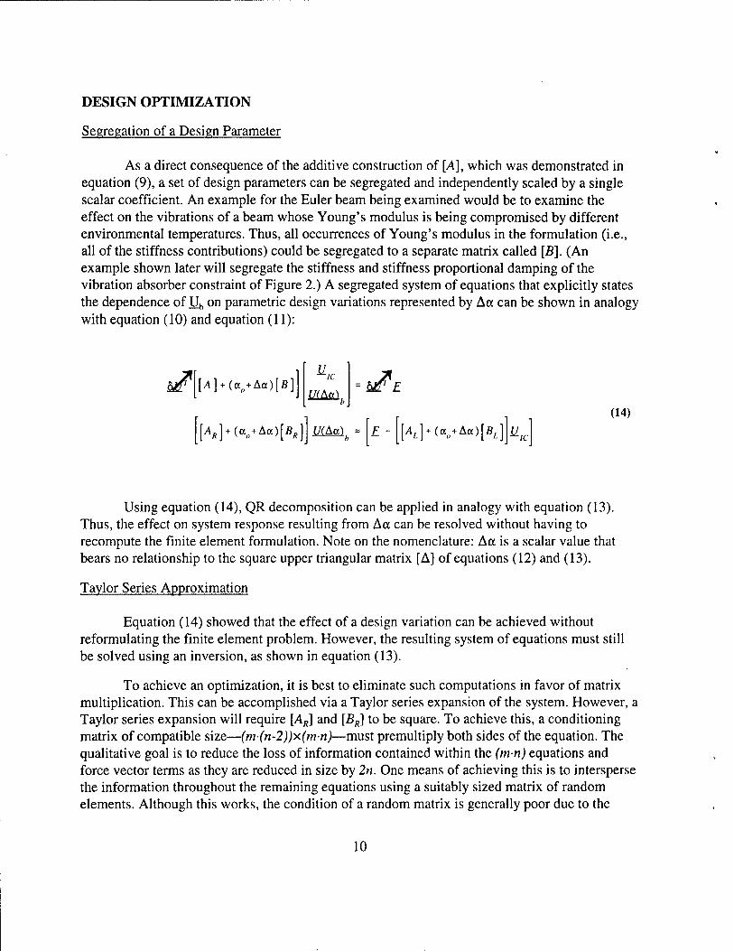
As a direct consequence of the additive construction of [A], which was demonstrated in equation (9), a set of design parameters can be segregated and independently scaled by a single scalar coefficient. An example for the Euler beam being examined would be to examine the effect on the vibrations of a beam whose Young's modulus is being compromised by different environmental temperatures. Thus, all occurrences of Young's modulus in the formulation (i.e., all of the stiffness contributions) could be segregated to a separate matrix called [B]. (An example shown later will segregate the stiffness and stiffness proportional damping of the vibration absorber constraint of Figure 2.) A segregated system of equations that explicitly states the dependence of Ub on parametric design variations represented by Aa can be shown in analogy with equation (10) and equation (11):

&T [i4] + (a0+A«)[ß] MAal h$i

M + «V*«)[**] JÄAfiÜ, * \E - [At] + (o0+Ao)[fit] 11 ic

(14)

Using equation (14), QR decomposition can be applied in analogy with equation (13). Thus, the effect on system response resulting from Aa can be resolved without having to recompute the finite element formulation. Note on the nomenclature: Aa is a scalar value that bears no relationship to the square upper triangular matrix [A] of equations (12) and (13).

Taylor Series Approximation

Equation (14) showed that the effect of a design variation can be achieved without reformulating the finite element problem. However, the resulting system of equations must still be solved using an inversion, as shown in equation (13).

To achieve an optimization, it is best to eliminate such computations in favor of matrix multiplication. This can be accomplished via a Taylor series expansion of the system. However, a Taylor series expansion will require [AR] and [BR] to be square. To achieve this, a conditioning matrix of compatible size—(m-(n-2))x(m-n)—must premultiply both sides of the equation. The qualitative goal is to reduce the loss of information contained within the (m-n) equations and force vector terms as they are reduced in size by 2n. One means of achieving this is to intersperse the information throughout the remaining equations using a suitably sized matrix of random elements. Although this works, the condition of a random matrix is generally poor due to the

10

inherent mix of large and small magnitudes of the elements. (Using the MATLAB <cond> command [ref 3], the condition of such a matrix with m = 82 and n = 7 is more than 3,000.) A second method is to intelligently pick a matrix whose elements consist of ones and minus ones. A suitably sized submatrix of a Hadamard matrix is very well-conditioned. (A condition of eight was found.) Finally, the [QT

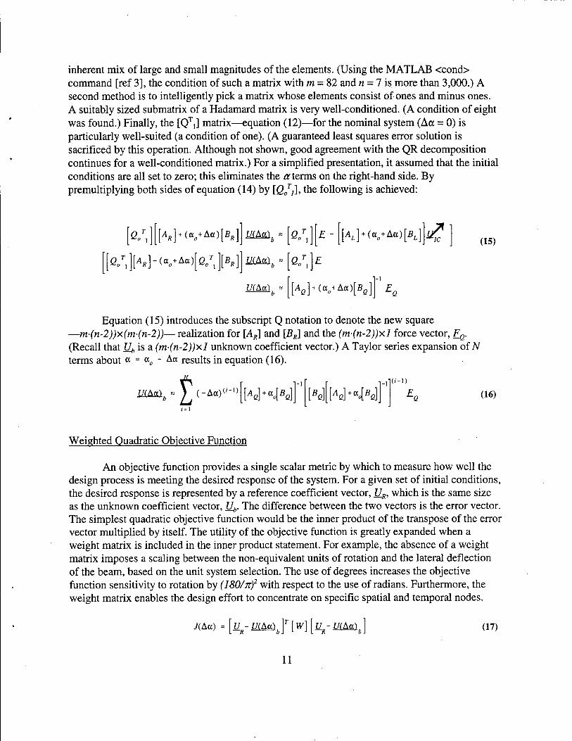
(] matrix—equation (12)—for the nominal system (Aa = 0) is particularly well-suited (a condition of one). (A guaranteed least squares error solution is sacrificed by this operation. Although not shown, good agreement with the QR decomposition continues for a well-conditioned matrix.) For a simplified presentation, it assumed that the initial conditions are all set to zero; this eliminates the a terms on the right-hand side. By premultiplying both sides of equation (14) by [Q0

T,], the following is achieved:

" I r

Q' [AÄ] + (a0+Aa)[BÄ] U(Aa)h * b Q ' £ -

fß T [AJ + (a0+Aa) QT \B«}] V(Av)h - QT £ J

U(Aa)

AL] + (ao+Aa)[BL]

AQ] + (afl+Aa)[BQ

if (15)

Equation (15) introduces the subscript Q notation to denote the new square —m-(n-2))x(m-(n-2))— realization for [AR] and [BR] and the (m-(n-2))xl force vector, FQ.

(Recall that U^ is a (m-(n-2))xl unknown coefficient vector.) A Taylor series expansion of iV terms about a = a0 + Aa results in equation (16).

MAaX I ;' = ]

(-Aa) O'-i) AcM*e. B, Ad+a4ßö (i-i)

(16)

Weighted Quadratic Objective Function

An objective function provides a single scalar metric by which to measure how well the design process is meeting the desired response of the system. For a given set of initial conditions, the desired response is represented by a reference coefficient vector, UR, which is the same size as the unknown coefficient vector, U^. The difference between the two vectors is the error vector. The simplest quadratic objective function would be the inner product of the transpose of the error vector multiplied by itself. The utility of the objective function is greatly expanded when a weight matrix is included in the inner product statement. For example, the absence of a weight matrix imposes a scaling between the non-equivalent units of rotation and the lateral deflection of the beam, based on the unit system selection. The use of degrees increases the objective function sensitivity to rotation by (180/'nf with respect to the use of radians. Furthermore, the weight matrix enables the design effort to concentrate on specific spatial and temporal nodes.

J(Ao) = [uR- U(Aa)b]T[W] [UR- U(Aa)J (17)

11

Finally, it must be noted that the objective function can be analytically formulated by incorporating equation (15) into equation (17). Therefore, its Jacobian can be readily computed in analogy with equation (16)—thereby enabling enhanced optimization algorithms such as cubic polynomial time searching (MATLAB's <fminu> command [ref 9]).

CASE STUDY: DESIGN OF A VIBRATION ABSORBER CONSTRAINT

The Design Objective

A straightforward design objective is to select the stiffness of the vibration absorber constraint of Figure 2 so that the beam and the coupled absorber are almost straight at a specific instant in time after the impulse. The vibration absorber coupling directly alters four elements of the spatial stiffness matrix of equation (1) (ref 8). Furthermore, the same indices of the damping matrix of equation (1) are also affected by the stiffness proportional damping. Thus, the vibration absorber constraint can be segregated from the damping and stiffness matrices of equation (1). Their separation can be maintained by adding the temporal finite element formulation of equation (9) so that the controlled coupling parameters are contained within [BQ] of equation (15), while [AQ] is totally devoid of their presence. The nominal value of the scalar design coefficient (a0) is set to one, with the remaining system parameters identical to those of Figure 2.

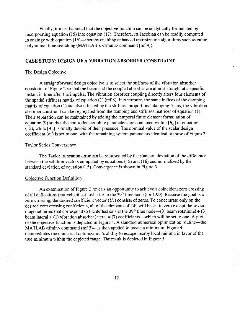
Taylor Series Convergence

The Taylor truncation error can be represented by the standard deviation of the difference between the solution vectors computed by equations (15) and (16) and normalized by the standard deviation of equation (15). Convergence is shown in Figure 3.

Objective Function Definition

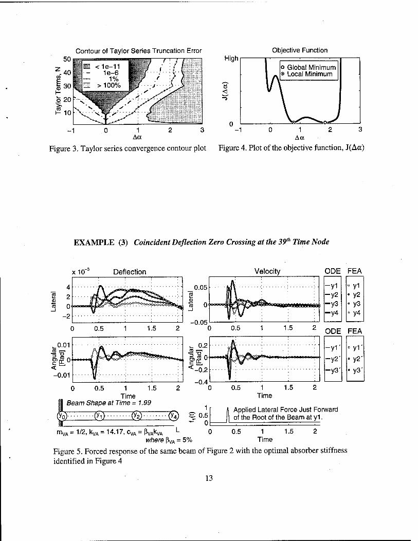
An examination of Figure 2 reveals an opportunity to achieve a coincident zero crossing of all deflections (not velocities) just prior to the 39th time node (t = 1.99). Because the goal is a zero crossing, the desired coefficient vector (UR) consists of zeros. To concentrate only on the desired zero crossing coefficients, all of the elements of [ W] will be set to zero except the seven diagonal terms that correspond to the deflections at the 39th time node—(3) beam rotational + (3) beam lateral + (1) vibration absorber lateral = (7) coefficients—which will be set to one. A plot of the objective function is depicted in Figure 4. A standard numerical optimization routine—the MATLAB <fmin> command (ref 3)—is then applied to locate a minimum. Figure 4 demonstrates the numerical optimization's ability to escape nearby local minima in favor of the true minimum within the depicted range. The result is depicted in Figure 5.

12

Contour of Taylor Series Truncation Error

-1 0 1 2 3 Aa

Figure 3. Taylor series convergence contour plot

High

8 <

Objective Function

o Global Minimum ® Local Minimum

1 Figure 4. Plot of the objective function, J(Aa)

EXAMPLE (3) Coincident Deflection Zero Crossing at the 39'" Time Node

x10" Deflection Velocity

_0.01

«got < " -0.01

0.5 1 1.5 Time

Beam Shape at Time = 1.99

W. M: mVA = 112, kVA = 14.17, cVA = ßVAkVA L

u. 0.2 CO r-,

<-0.2

-0.4 I

1 S 0.5 "^ 0

0.5 1 Time

1.5

ODE FEA

-yi o y1

-y2 o y2

-y3 • y3 -y4 o y4

ODE FEA

-y1' o y1'

-y2' o y2'

-y3' • y3'

Applied Lateral Force Just Forward of the Root of the Beam at y1.

0 0.5 1 1.5 2 where ßVA = 5% Time

Figure 5. Forced response of the same beam of Figure 2 with the optimal absorber stiffness identified in Figure 4

13

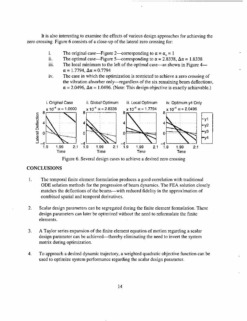
It is also interesting to examine the effects of various design approaches for achieving the zero crossing. Figure 6 consists of a close-up of the lateral zero crossing for:

i. The original case—Figure 2—corresponding to a = a0 = 1 ii. The optimal case—Figure 5—corresponding to a = 2.8338, Aa = 1.8338 iii. The local minimum to the left of the optimal case—as shown in Figure 4—

a =1.7794, Act = 0.7794 iv. The case in which the optimization is restricted to achieve a zero crossing of

the vibration absorber only—regardless of the six remaining beam deflections, a = 2.0496, Aa = 1.0496. (Note: This design objective is exactly achievable.)

i. Original Case ii. Global Optimum iii. Local Optimum iv. Optimum y4 Only

x-ICT4 a =1.0000 x10"4 a = 2.8338 x 10"4 a = 1.7794 x 10~4 a = 2.0496

1.9 1.99 Time

8

4

0

-4 H^

yi y2

y4

2.1 1.9 1.99 2.1 1.9 1.99 2.1 1.9 Time Time

Figure 6. Several design cases to achieve a desired zero crossing

1.99 2.1 Time

CONCLUSIONS

1. The temporal finite element formulation produces a good correlation with traditional ODE solution methods for the progression of beam dynamics. The FEA solution closely matches the deflections of the beams—with reduced fidelity in the approximation of combined spatial and temporal derivatives.

2. Scalar design parameters can be segregated during the finite element formulation. These design parameters can later be optimized without the need to reformulate the finite elements.

3. A Taylor series expansion of the finite element equation of motion regarding a scalar design parameter can be achieved—thereby eliminating the need to invert the system matrix during optimization.

4. To approach a desired dynamic trajectory, a weighted quadratic objective function can be used to optimize system performance regarding the scalar design parameter.

14

Final Notes

There is no inherent limitation of the method to a single design parameter. Multi- parameter optimization would be greatly enhanced by the analytic formulation of the objective function and the subsequent availability of a readily computed Jacobian.

There is no inherent limitation of the design method to the system parameters. Open-loop control can be enabled via design with respect to applied force. It is clear that an efficient basis for the control force representation would greatly increase the pragmatic implementation of such a design.

The potential to impose desired final conditions and solve for required initial conditions may exist.

15

REFERENCES

1. Simkins, T. E., "Finite Elements for Initial Value Problems in Dynamics," AJAA Journal, V19.N10, 1981, pp. 1357-1362.

2. Junkins, J. L., and Kim, Y., Introduction to Dynamics and Control of Flexible Structures, AIAA, Washington, 1993.

3. MATLAB Reference Guide, The Mathworks, Inc., Natick, MA, 1992.

4. Control System Toolbox: For Use with MATLAB, The Mathworks, Inc., Natick, MA, 1992.

5. Kathe, E. L., "MATLAB Modeling of Non-Uniform Beams Using the Finite Element Method for Dynamic Design and Analysis," U.S. Army Armament Research, Development and Engineering Center, Close Combat Armaments Center, Benet Laboratories, Technical Report ARCCB-TR-96010, Watervliet, NY, April 1996.

6. Johnson, C, Numerical Solution of Partial Differential Equations by the Finite Element Method, Cambridge University Press, Lund, Sweden, 1995.

7. Meirovitch, L., Methods of Analytical Dynamics, McGraw-Hill, New York, 1988.

8. Kathe, E. L., "Design and Validation of a Gun Barrel Vibration Absorber," Proceedings of the 67th Shock and Vibration Symposium, Vol. 1, 1996, pp. 447-456. Also available as: U.S. Army Armament Research, Development and Engineering Center, Close Combat Armaments Center, Benet Laboratories, Technical Report ARCCB-TR-97012, Watervliet, NY, May 1997.

9. Optimization Toolbox: For Use with MATLAB, The Mathworks, Inc., Natick, MA, 1994.

16

TECHNICAL REPORT INTERNAL DISTRIBUTION LIST

NO. OF COPIES

CHIEF, DEVELOPMENT ENGINEERING DIVISION ATTN: AMSTA-AR-CCB-DA 1

-DB 1 -DC 1 -DD 1 -DE 1

CHIEF, ENGINEERING DIVISION ATTN: AMSTA-AR-CCB-E 1

-EA 1 -EB 1 -EC 1

CHIEF, TECHNOLOGY DIVISION ATTN: AMSTA-AR-CCB-T 2

-TA 1 -TB 1 -TC 1

TECHNICAL LIBRARY ATTN: AMSTA-AR-CCB-0 5

TECHNICAL PUBLICATIONS & EDITING SECTION ATTN: AMSTA-AR-CCB-0 3

OPERATIONS DIRECTORATE ATTN: SIOWV-ODP-P 1

DIRECTOR, PROCUREMENT & CONTRACTING DIRECTORATE ATTN: SIOWV-PP 1

DIRECTOR, PRODUCT ASSURANCE & TEST DIRECTORATE ATTN: SIOWV-QA 1

NOTE: PLEASE NOTIFY DIRECTOR, BENET LABORATORIES. ATTN: AMSTA-AR-CCB-0 OF ADDRESS CHANGES.

TECHNICAL REPORT EXTERNAL DISTRIBUTION LIST

ASST SEC OF THE ARMY RESEARCH AND DEVELOPMENT ATTN: DEPT FOR SCI AND TECH THE PENTAGON WASHINGTON, D.C. 20310-0103

DEFENSE TECHNICAL INFO CENTER ATTN: DTIC-OCP (ACQUISITIONS) 8725 JOHN J. KINGMAN ROAD STE 0944 FT. BELVOIR. VA 22060-6218

COMMANDER U.S. ARMY ARDEC ATTN: AMSTA-AR-AEE, BLDG. 3022

AMSTA-AR-AES, BLDG. 321 AMSTA-AR-AET-O, BLDG. 183 AMSTA-AR-FSA, BLDG. 354 AMSTA-AR-FSM-E AMSTA-AR-FSS-D, BLDG. 94 AMSTA-AR-IMC, BLDG. 59

P1CATINNY ARSENAL, NJ 07806-5000

DIRECTOR U.S. ARMY RESEARCH LABORATORY ATTN: AMSRL-DD-T, BLDG. 305 ABERDEEN PROVING GROUND, MD

21005-5066

DIRECTOR U.S. ARMY RESEARCH LABORATORY ATTN: AMSRL-WT-PD (DR. B. BURNS) ABERDEEN PROVING GROUND, MD

21005-5066

NO. OF NO. OF COPIES

COMMANDER ROCK ISLAND ARSENAL

COPIES

1 ATTN: SMCRI-SEM ROCK ISLAND, IL 61299-5001

1

COMMANDER U.S. ARMY TANK-AUTMV R&D COMMAND ATTN: AMSTA-DDL (TECH LIBRARY) 1 WARREN, MI 48397-5000

COMMANDER U.S. MILITARY ACADEMY ATTN: DEPARTMENT OF MECHANICS 1 WEST POINT, NY 10966-1792

U.S. ARMY MISSILE COMMAND REDSTONE SCIENTIFIC INFO CENTER 2 ATTN: AMSMI-RD-CS-R/DOCUMENTS

BLDG. 4484 REDSTONE ARSENAL, AL 35898-5241

COMMANDER U.S. ARMY FOREIGN SCI & TECH CENTER ATTN: DRXST-SD 1 220 7TH STREET, N.E. CHARLOTTESVILLE. VA 22901

COMMANDER U.S. ARMY LABCOM, ISA ATTN: SLCIS-IM-TL 1 2800 POWER MILL ROAD ADELPHI, MD 20783-1145

NOTE: PLEASE NOTIFY COMMANDER, ARMAMENT RESEARCH. DEVELOPMENT, AND ENGINEERING CENTER, BENET LABORATORIES, CCAC. U.S. ARMY TANK-AUTOMOTIVE AND ARMAMENTS COMMAND.

AMSTA-AR-CCB-O. WATERVLIET, NY 12189-4050 OF ADDRESS CHANGES.

TECHNICAL REPORT EXTERNAL DISTRIBUTION LIST (CONT'D)

NO. OF COPIES

NO. OF COPIES

COMMANDER U.S. ARMY RESEARCH OFFICE ATTN: CHIEF, IPO P.O. BOX 12211 RESEARCH TRIANGLE PARK, NC 27709-2211

DIRECTOR U.S. NAVAL RESEARCH LABORATORY ATTN: MATERIALS SCI & TECH DIV WASHINGTON, D.C. 20375

WRIGHT LABORATORY ARMAMENT DIRECTORATE ATTN: WL/MNM EGLIN AFB, FL 32542-6810

WRIGHT LABORATORY ARMAMENT DIRECTORATE ATTN: WL/MNMF EGLIN AFB, FL 32542-6810

NOTE: PLEASE NOTIFY COMMANDER, ARMAMENT RESEARCH, DEVELOPMENT, AND ENGINEERING CENTER, BENET LABORATORIES, CCAC, U.S. ARMY TANK-AUTOMOTIVE AND ARMAMENTS COMMAND,

AMSTA-AR-CCB-O, WATERVLIET, NY 12189-4050 OF ADDRESS CHANGES.