Embed Size (px)
Citation preview
U.S. Cotton Prices and the World Cotton Market: Forecasting and Structural Change
Olga Isengildina-Massa and Stephen MacDonald1
Selected Paper prepared for presentation at the American Agricultural Economics Association Annual Meeting, Milwaukee, Wisconsin, July 25-29, 2009
Copyright 2009 by Olga Isengildina and Stephen MacDonald. All rights reserved. Readers may make verbatim copies of this document for non-commercial purposes by any means, provided
that this copyright notice appears on all such copies.
*Assistant Professor in the Department of Applied Economics and Statistics at Clemson University and Senior Economist Economic Research Service, respectively. The authors appreciate the research assistance of Michael D. Scott, the Graduate Student at Clemson University. The funding support of the U.S. Department of Agriculture under Cooperative Agreement 58-3000-7-0063 is gratefully acknowledged. Any opinions, findings, conclusions, or recommendations expressed in this document are those of the authors and do not necessarily reflect the view of the U.S. Department of Agriculture.
brought to you by COREView metadata, citation and similar papers at core.ac.uk
provided by Research Papers in Economics
2
U.S. Cotton Prices and the World Cotton Market:
Forecasting and Structural Change
Introduction
Agricultural prices are notoriously difficult to forecast due to shocks from weather events around
the world, the important role of government policy in the marketplace, and changing tastes and
technology. In addition, agricultural prices are affected by the shocks affecting the rest of the
economy, including macroeconomic policy and shifts in energy markets. Forecasts of
agricultural prices are important to both private and public policy-makers, as well producers and
consumers of agricultural products. Therefore, agricultural price forecasting is a widespread
activity. USDA alone publishes updates of price forecasts for 24 commodities every month in its
World Agricultural Supply and Demand Estimates. However, until recently USDA was legally
prohibited from forecasting cotton prices.2 Cotton price forecasts were available each month
from the International Cotton Advisory Committee (ICAC) and—with less frequent updates—
from the Food and Agricultural Policy Research Institute (FAPRI), the Australian Bureau of
Agricultural and Resource Economics (ABARE), and the World Bank. In addition, although
USDA did not publish cotton price forecasts, the USDA’s Interagency Commodity Estimates
Committee (ICEC) for cotton calculated unpublished estimates of world and domestic cotton
prices each month. In recent years, USDA and other agencies have observed systematic errors in
their cotton price forecasting models, highlighting the need for a thorough review of price
relationships. The removal of the ban on cotton price forecasting by USDA in the 2008 Farm
Bill has made the need to review existing cotton price forecasting procedures and develop of a
new forecasting model an urgent one.
2 In 1929, Congress passed legislation forbidding USDA from publishing cotton price forecasts (see Townsend (1989) for a discussion of the circumstances surrounding this legislation).
3
This paper develops a theoretically-based reduced-form specification for a cotton price
forecasting model. Like earlier models for cotton (Meyer, 1998; Valderrama, 1993; Goreux, et
al., 2007)), wheat (Westcott and Hoffman, 1999), corn (Van Meir, 1983; Westcott and Hoffman,
1999), and soybeans (Plato and Chambers, 2004; Goodwin, Schnepf, and Dohlman, 2005), the
U.S. season-average farm price is a function of U.S. stocks/use. Other variables include U.S. and
world cotton supply and a set of shift variables accommodating circumstances particular to
cotton markets. The empirical version of the model includes a demand shifter for China’s trade
and another shifter for the impact of U.S. commodity policy. Testing indicates evidence of
structural change, which is likely the result of the U.S. shift from domestic cotton consumption
to exporting, and the model is adjusted to include impacts of foreign supply.3
Data
This study concentrates on the marketing year average U.S. farm price of upland cotton, with the
historical data over 1973 through 2007 collected from the USDA’s National Agricultural
Statistics Service (NASS) database and publications (USDA-NASS, 2008). One-year-ahead
forecasts for U.S., world, and China supply and use categories are published in monthly USDA
World Agricultural Supply and Demand Estimates (WASDE) reports from the USDA’s World
Agricultural Outlook Board (USDA-WAOB, 2008). These forecasts will provide the out-of-
sample values for the independent variables in future years. The data for the past realizations of
cotton supply and demand were drawn from the “Production, Supply and Distribution Online”
database maintained by USDA’s Foreign Agricultural Service (USDA-FAS, 2008). Unlike
wheat and feed grains, USDA does not publish forecasts and historical estimates of Commodity
3 Foreign supply is an important factor for U.S. cotton prices because the United States is one of the largest producers and exporters of cotton in the world market and as such directly competes with cotton coming from other countries.
4
Credit Corporation (CCC) end of year stocks in the monthly WASDE. CCC cotton stocks are
forecast twice a year in order to project budgetary outlays, and historical data for CCC cotton
stocks were provided by USDA’s Farm Service Agency (FSA). Data on expenditures for the
U.S. User Market Certificate Program (“Step 2”) were also provided by FSA. Since the “Step 2”
program ended in August 2006, forecasts will not be necessary for future years.
Cotton Price Model
Theoretical Model
The general framework for the cotton price model presented in this study is based on the theory
of competitive markets in which market price results from allocating available supplies to
alternative product uses (e.g., Tomek and Robinson, 2003, p. 406). For the U.S. cotton markets
the identity between supply and demand can be written as:
(1) 1t t t t t tI Q X I A M−+ + = + +
where It = ending inventory,
It-1 = beginning inventory,
Qt = domestic consumption,
Xt = exports,
At = domestic production, and
Mt = imports.
At the beginning of the marketing year denoted by t, the variables on the right-hand side can be
treated as predetermined4. Therefore, the above identity results in the demand for domestic uses,
the demand for exports, and the demand for inventories at a given level of supply. To simplify,
4 Imports are not predetermined, but are trivially small compared with production.

5
the demand for domestic uses and the demand for exports may be summed to represent current
demand (Dt). Similarly, the sum of beginning inventory, domestic production and imports
reflects current supply (St). This allows the identity to be expressed as:
(2) 0t t tS D I− − = .
Each variable in the identity is a function of a set of explanatory variables as written below:
( ( ), )t t tS b E p z=
( , )t t tD g p y=
( , )t t tI h p w=
where pt is the inflation-adjusted price, E(pt) is expected price, zt, yt, and wt are exogenous
variables affecting supply, demand, and stocks, respectively and all other variables are as defined
previously. Supply is positively related to expected price while demand and stocks are
negatively related to price. Assuming that supply is predetermined at the beginning of the
marketing year, equation 2 can be expressed as:
(3) ( , ) ( , ) 0t t t t tS g p y h p w− − =
Traditionally, in forecasting models price is specified as a function of stocks-to-use ratio (e.g.,
Westcott and Hoffman, 1999). Stocks-to-use ratio can be introduced in equation 3 by dividing
through by g(pt, yt):
(4) ( , )1 ( , , )( , ) ( , )
t t tt t t
t t t t
S h p w r p w yg p y g p y
− = =
Where r denotes the ratio of stocks-to use. Equation 4 is the implicit price equation. To find an
explicit equation for price we differentiate equation 45:
5 Since time (t) indicator is identical for all variables, it is omitted from the following mathematical derivations.
6
(5) ( ) g g g gdS dr g dp dy dp dy rp y p y
⎛ ⎞∂ ∂ ∂ ∂= + + + +⎜ ⎟∂ ∂ ∂ ∂⎝ ⎠
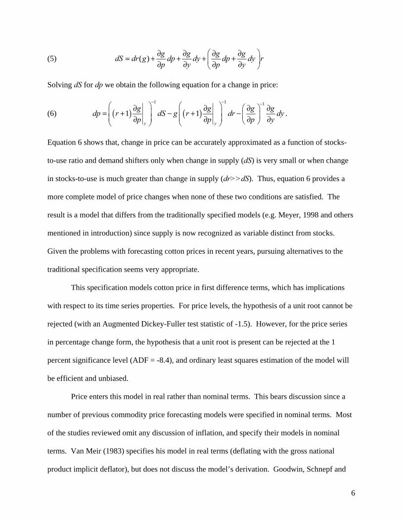
Solving dS for dp we obtain the following equation for a change in price:
(6) ( ) ( )1 1 1
1 1y y
g g g gdp r dS g r dr dyp p p y
− − −⎛ ⎞ ⎛ ⎞ ⎛ ⎞∂ ∂ ∂ ∂⎜ ⎟ ⎜ ⎟= + − + − ⎜ ⎟⎜ ⎟ ⎜ ⎟∂ ∂ ∂ ∂⎝ ⎠⎝ ⎠ ⎝ ⎠
.
Equation 6 shows that, change in price can be accurately approximated as a function of stocks-
to-use ratio and demand shifters only when change in supply (dS) is very small or when change
in stocks-to-use is much greater than change in supply (dr>>dS). Thus, equation 6 provides a
more complete model of price changes when none of these two conditions are satisfied. The
result is a model that differs from the traditionally specified models (e.g. Meyer, 1998 and others
mentioned in introduction) since supply is now recognized as variable distinct from stocks.
Given the problems with forecasting cotton prices in recent years, pursuing alternatives to the
traditional specification seems very appropriate.
This specification models cotton price in first difference terms, which has implications
with respect to its time series properties. For price levels, the hypothesis of a unit root cannot be
rejected (with an Augmented Dickey-Fuller test statistic of -1.5). However, for the price series
in percentage change form, the hypothesis that a unit root is present can be rejected at the 1
percent significance level (ADF = -8.4), and ordinary least squares estimation of the model will
be efficient and unbiased.
Price enters this model in real rather than nominal terms. This bears discussion since a
number of previous commodity price forecasting models were specified in nominal terms. Most
of the studies reviewed omit any discussion of inflation, and specify their models in nominal
terms. Van Meir (1983) specifies his model in real terms (deflating with the gross national
product implicit deflator), but does not discuss the model’s derivation. Goodwin, Schnepf and
7
Dohlman consider the role of inflation, and test specifications with inflation as an independent
variable in their model, which forecasts nominal prices. Both including inflation as a variable
and forecasting a deflated price when the ultimate goal is a nominal price forecast put the
forecaster’s results at the mercy of the available forecasts of inflation. However, if inflation
should be accounted for, a model that completely omits it will see its usefulness diminished in
other ways.
Given that this model’s reduced form is based on a theoretical model with predetermined
supply but demand as a function of price, real rather than nominal prices are the appropriate
dependent variable. Demand is almost invariably modeled as a function of real rather than
nominal prices (see Ferris, 1998), and a broad measure of inflation was chosen since cotton
products will be competing with a broad range of products for consumer demand. Furthermore,
given that the nominal loan rate is not an independent variable in this model, the use of real
prices does not adversely affect the role of the independent variables as it would for some of the
earlier models.
Empirical Analysis
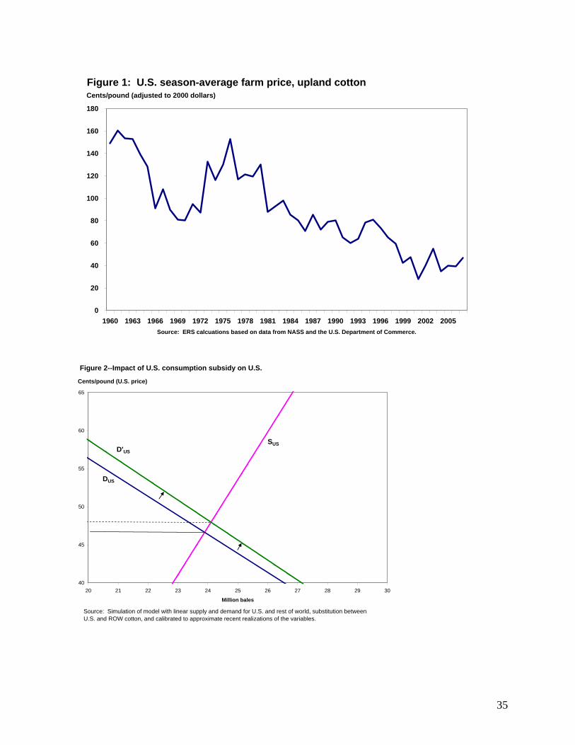
Figure 1 shows changes in the U.S. marketing year average farm price of upland cotton over
1960/61 though 2006/07. This figure shows that U.S. cotton price has been highly variable over
time under the pressure of various economic and political factors. Equation 7 provides a reduced
form model for evaluating percent changes in U.S. average farm price (dp) based on changes in
U.S. supply (dS), U.S. stocks-to-use ratio (dr), and a set of demand shifters. A demand shifter
that appears perhaps most relevant during the period of study is export demand associated with
China’s trade policy. The strong correlation between world cotton prices and China’s net trade
8
was noted as early as 1988 by the ICAC, and the level of China’s net trade was included in the
ICAC’s world price forecasting model for the 1974/75 through 1986/87 period (ICAC, 1988).
Similarly, MacDonald (1998) adjusted the world (minus China) stocks-to-use variable by the
amount of China’s net trade in another world price model, estimated using 1971/72 through
1995/96 data. In 2001, USDA highlighted how China’s domestic cotton policy drove its cotton
trade, with significant impacts on world markets:
“Stocks rose after 1994/95 as China raised its farm prices while maintaining an open trade regime. China’s government-mandated farm prices proved difficult to reduce as world prices fell, and restricting imports seemed inconsistent with ensuring the profitability of its huge textile industry. Also, government policy locked older cotton in stocks in order to prevent bookkeeping losses as the market value of procured cotton tumbled below the cost of purchasing, processing, and storage. Stocks reached a staggering 106 percent of use in 1998/99, and China accounted for 47 percent of the entire world’s cotton ending stocks. Then, starting in 1998/99, the government began applying quantitative restrictions to cotton imports and subsidizing exports. In 1999/2000 the government effectively cut farm prices by refusing to guarantee procurement, and in 2000/01 a program to allow the central government to absorb the cost of marketing losses for stockpiled cotton went into high gear, opening the floodgates for enormous government stocks to flow into the market. By 2000/01, China had cut its ending stocks by nearly 10 million bales, mostly from government stocks (Market and Trade Economics Division, 2001).”
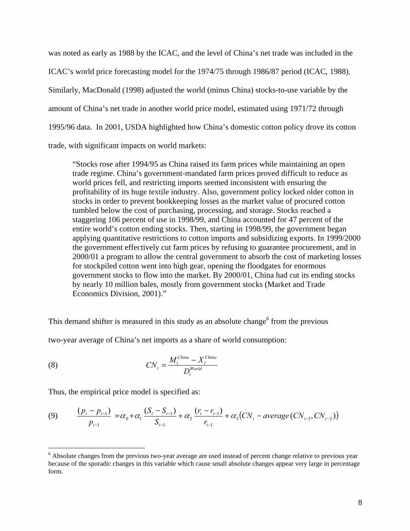
This demand shifter is measured in this study as an absolute change6 from the previous
two-year average of China’s net imports as a share of world consumption:
(8) Worldt
Chinat
Chinat
t DXMCN −=
Thus, the empirical price model is specified as:
(9) ( )),()()()(213
1
12
1
110
1
1−−
−
−
−
−
−
− −+−+−+=−ttt
t
tt
t
tt
t
tt CNCNaverageCNr
rrS
SSp
pp αααα
6 Absolute changes from the previous two-year average are used instead of percent change relative to previous year because of the sporadic changes in this variable which cause small absolute changes appear very large in percentage form.
9
where all variables refer to U.S. values unless stated otherwise. Since supply is predetermined,
changes in supply have an inverse effect on price. Changes in stocks-to-use ratio are also
negatively related to price. Greater China net imports represent a greater export demand for U.S.
cotton and thus have a positive relationship with price changes.
Another factor affecting the relationship between U.S. ending stocks and prices is
government policy. The two most relevant policies to cotton prices are the loan program and the
User Marketing Certificate Program (generally referred to as “Step 2” of the marketing loan
program) (see Meyer, MacDonald, and Foreman, 2007, for a summary of U.S. farm programs
affecting cotton). Since the relationship between how the loan program affects prices and how
stocks affect prices in this model is relatively straightforward, a simple demand shifter can be
created to account for the loan program. Step 2’s effects were accounted for by adjusting the
dependent variable for its impacts.
Before 1986, U.S. commodity programs sometimes served to establish a price floor for
U.S. crops. USDA’s Commodity Credit Corporation (CCC) acquired large stocks of cotton (and
other commodities) during the early 1980’s as market prices in the United States fell below U.S.
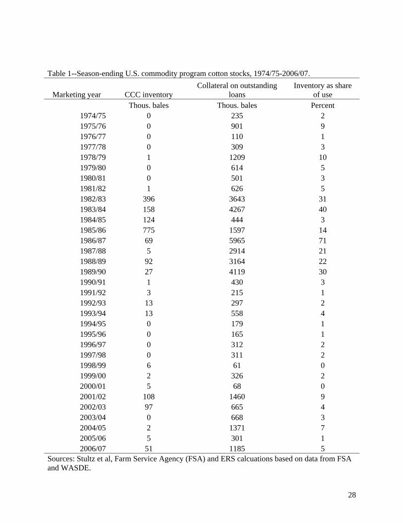
loan rates (Table 1). Stocks owned by CCC were not available to the market, and prices were
higher than if the stocks could have been drawn upon to satisfy demand. Furthermore, even
cotton that had not yet been acquired by CCC, but was still being used as collateral in the loan
program, was also not freely available for spinning, export, or private stockholding. The
adjustment of the U.S. cotton program to a marketing loan meant that CCC acquisition of cotton
was significantly reduced, and in 2006 CCC instituted a policy of immediately selling any
forfeited cotton, ensuring CCC stocks remain essentially at zero at the end of the marketing year.
However, the ability of producers to place their cotton in the loan program still affected prices
10
after 1986, and the volume of cotton remaining as collateral in the loan program at the end of the
marketing year was often significant, even in recent years. If cotton under loan has not been
acquired by CCC, then the maximum duration of its stay under loan is 9 months. Given that
cotton continues to enter the loan in the months after January of each year, cotton can remain
under loan for several months after the end of the marketing year. Note also that unlike with
grains, storage costs are covered by the CCC when the redemption price applicable to the loan is
below the loan rate. This further enhances the incentive of producers to delay marketing their
cotton when the loan program is a sound alternative.
Therefore, a variable was created representing the sum of both cotton owned by CCC and
of cotton with CCC loans still outstanding as of the end of the marketing year. This was divided
by cotton use for that year to create an additional demand shifter:
(10) t
loant
CCCt
t DhhCCC +=
where CCCth is the cotton owned by CCC at the end of the marketing year and loan
th is the volume
of cotton remaining as collateral in the loan program at that time. By capturing all of the cotton
involved in the loan program instead of the just the cotton owned by CCC, the variable more
accurately captures how the loan program supports prices. The loan rate appears to have
functioned as price floor in 1981, 1982, and 1984, but stocks from cotton produced in that
marketing year were not acquired by CCC until the next marketing year. In order to capture the
functioning of the loan program in those years, the actual loan rate or another variable would
have to be added (as in Westcott and Hoffman, 1999). Equation 10 allows the impact of the loan
program to be accounted for with one variable.
11
Another government policy that affected cotton markets is the U.S. Step 2 program,
which was introduced in the 1990 U.S. farm legislation. The Step 2 program offered payments
to U.S. textile mills and U.S. exporters when the price of U.S. cotton in Northern Europe
exceeded the world price of cotton, also measured in Northern Europe. A World Trade
Organization (WTO) panel found the program in violation of the General Agreement on Trade
and Tariffs (GATT), in large part because the payments to U.S. mills were exclusively for the
consumption of U.S. cotton rather than either U.S. or imported cotton (see Schnepf, 2007, for a
summary of the dispute). In the program’s early years, the seasonality of price spread that
determined Step 2 payments and the seasonality of U.S. export sales coincided. Therefore,
exports accounted for a disproportionate share of the payments in those years. The ability of
exporters to lock in payments for much of the year’s exports within a relatively small window of
time was also a factor. As a result, Step 2 was often perceived to be primarily an export subsidy.
However, regulatory changes in the program were frequent, and domestic U.S. payments
exceeded payments to exporters in later years.
During much of the program’s tenure, payments to exporters were effected at the time of
shipment rather than sale. Sales for exports typically occur 9-10 weeks before shipment, and
occasionally substantially further in advance. Since the magnitude of Step 2 payments fluctuated
weekly, this added uncertainty to the relationship between the price of export sales and the
subsidy associated with the shipment. When this is taken into account along with the fact that
payments were made to the firms exporting the cotton rather than purchasing it, the link between
Step 2 payment and subsidization of export demand is not as direct as it could be. However, the
subsidies were non-trivial, equaling 5 percent of the value of U.S. cotton use on average during
1991-2006. Given that U.S. cotton accounted for about 20 percent of global cotton use during
12
this time, it is reasonable to expect that the program had an impact on world price as well as U.S.
price. The Step 2 program was terminated in August 2006 as part of the United States’ efforts to
comply with the WTO panel’s findings. Step 2 therefore is no longer a factor in the
determination of prices, but is nonetheless a factor to be accounted for in any analysis relying on
historical data.
The simplest way to understand the impact of the Step 2 program is to abstract from the
differing effects on U.S. export and domestic demand and simply consider it as a subsidy for
consumption of U.S. cotton (Figures 2 and 3). The introduction of the subsidy would shift the
demand for U.S. cotton upward from DUS to D`US, and the demand for the rest of the world’s
(ROW) cotton downward from DROW to D`ROW. The new equilibrium would have production
and consumption of U.S. cotton slightly higher than in the absence of a subsidy, and slightly
lower for ROW. Similarly, the U.S. price of cotton would be higher, and would rise to a greater
degree than the decline in the ROW’s price. Simulations by FAPRI (2005) and Mohanty, et al.
(2005) found such an impact, with the two studies predicting on average that removing Step 2
would mean a 2.9 percent lower U.S. price and a less than 1 percent higher world price. Since
Step 2 will no longer be a factor in U.S. prices, and since it influenced past prices, the forecasting
model was estimated with data for the dependent variable adjusted to remove the past impact of
Step 2. Data on spending for Step 2 payments in each year was divided by the level of U.S.
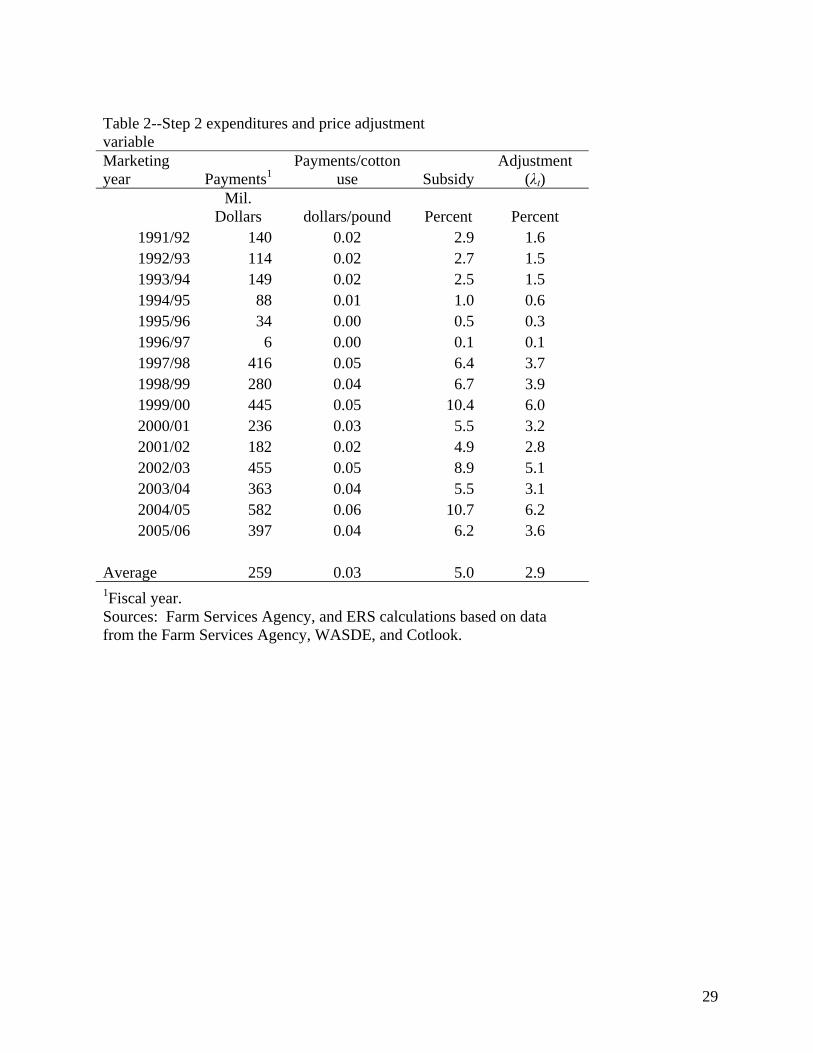
cotton use to determine the relative subsidy provided each year (Table 2). An adjustment
variable (λ t) was constructed so that each year’s adjustment was proportional to that year’s
subsidy, and the average value of the adjustments over 1991-2005 was -2.9 percent. This
variable was used to adjust the U.S. season-average upland farm price to remove the impact of
Step 2.

13
(11) t
NASStt
tt
NASSt
t GDPDEFppand
GDPDEFpp )1(* λ−==
Here we define pt more explicitly as the season-average price reported by USDA’s National
Agricultural Statistics Service ( )NASStp , deflated by U.S. Department of Commerce’s gross
domestic product price index (GDPDEFt).
Thus, the cotton price model adjusted for the impact of the government programs is:
(12) ( ) ttttt
tt
t
tt
t
tt CCCCNCNaverageCNr
rrS
SSp
pp4213
1
12
1
110*
1
*1
*
),()()()( ααααα +−+−+−+=−−−
−
−
−
−
−
−
Other factors that may have an important effect on cotton prices include energy prices.
Previous work (e.g. Barsky and Kilian, 2002) has indicated how oil price shocks can affect prices
in general. More recently, policy changes have linked energy and grain prices (Westcott, 2007).
Energy market shocks occurred in the 1970’s and again after 2004. In an effort to develop a
model that is robust to both high and low energy prices, and to a variety of policy environments,
this study concentrates on cotton price movements starting from the 1974/75 marketing year and
extending to 2007/08. Since the proposed model is estimated in reduced form, the impact of
energy prices is included implicitly through the supply variable. A similar argument can be
made about other supply inducing variables, such as the price of cotton seed.
Structural Change Test
Following Wang and Tomek (2007) it is important to insure that a correctly specified model is
used to test for structural change. Therefore, equation 12 is used to test for structural change. A
traditional approach would be to pick an arbitrary sample breakpoint, often the midpoint of the
sample, and use a Chow test for structural change. This could be further refined by associating
breakpoints with major events relevant to the data series. Either of these approaches suffers from

14
the arbitrary nature of the selected breakpoints. Recent literature suggests the Quandt-
Likelihood Ratio (QLR) test is superior test for detecting structural change of unknown timing
(e.g., Hansen, 2001). The QLR test consists of calculating Chow breakpoint test at every
observation, while making sure that subsample points are not too close to the end points of the
sample. The QLR test was applied to the pooled data in this study with 20% trimming. The
highest value of the QLR statistic was 5.0 (figure 4). The probabilities for these statistics were
calculated using Hansen’s (1997) method. The critical values of the QLR statistic at the 99%
significance level with five restrictions is 4.53 (Stock and Watson, p. 471), which indicates that
the null hypothesis of no structural change is rejected. The maximum statistic of 5.0 was
observed in 1999/00, which indicates the breakpoint location.
This structural break was likely caused by a combination of factors. Besides significant
changes in international trade discussed earlier, which have been transitory in nature, this period
coincided with some permanent fundamental regime changes in China’s supply due to the end of
guaranteed procurement prices. Some permanent changes also took place in China’s
consumption sector due to its growing textile industry. These regime changes in China’s cotton
sector are likely associated with China’s accession to the WTO at the end of 2001. China joined
the WTO just as the textile trade liberalization provisions of the Uruguay Round Agreement
were having an impact. The phasing-out of developed country textile trade protection
(commonly referred to as Multifiber Arrangement, or MFA) was an important factor behind the
rapid increased export orientation of the US cotton industry. Figure 5 shows that in the early
2000s export demand surpassed domestic use of the U.S. upland cotton. As the export share of
U.S. cotton use rose to levels not seen since the 19th century, the importance of world supply and
demand to U.S. cotton prices increased.
15
In order to correct for the structural change detected in the estimated model (equation 12)
an additional shift variable was included in the model to reflect an increased export orientation of
the US cotton industry. The world market signals are assumed to be transmitted to the US
market through the foreign supply, which was constructed excluding China’s supply, but
including China’s net contribution to the global availability of cotton (net exports)7:
(13) Chinat
Chinat
Chinat
Foreignt
Foreignt MXSSS −+−=
Foreign supply is an important factor for U.S. cotton prices because the United States is one of
the largest producers and exporters of cotton and as such directly competes with cotton coming
from other countries. With this variable included, no structural break was detected and the
specification of the model was complete. Thus, the final model specification is:
(14)( )
( )Foreignt
Foreignt
Foreignt
ttttt
tt
t
tt
t
tt
SSS
CCCCNCNaverageCNr
rrS
SSp
pp
1
15
42131
12
1
110*
1
*1
*
),()()()(
−
−
−−−
−
−
−
−
−
−+
+−+−+−+=−
α
ααααα
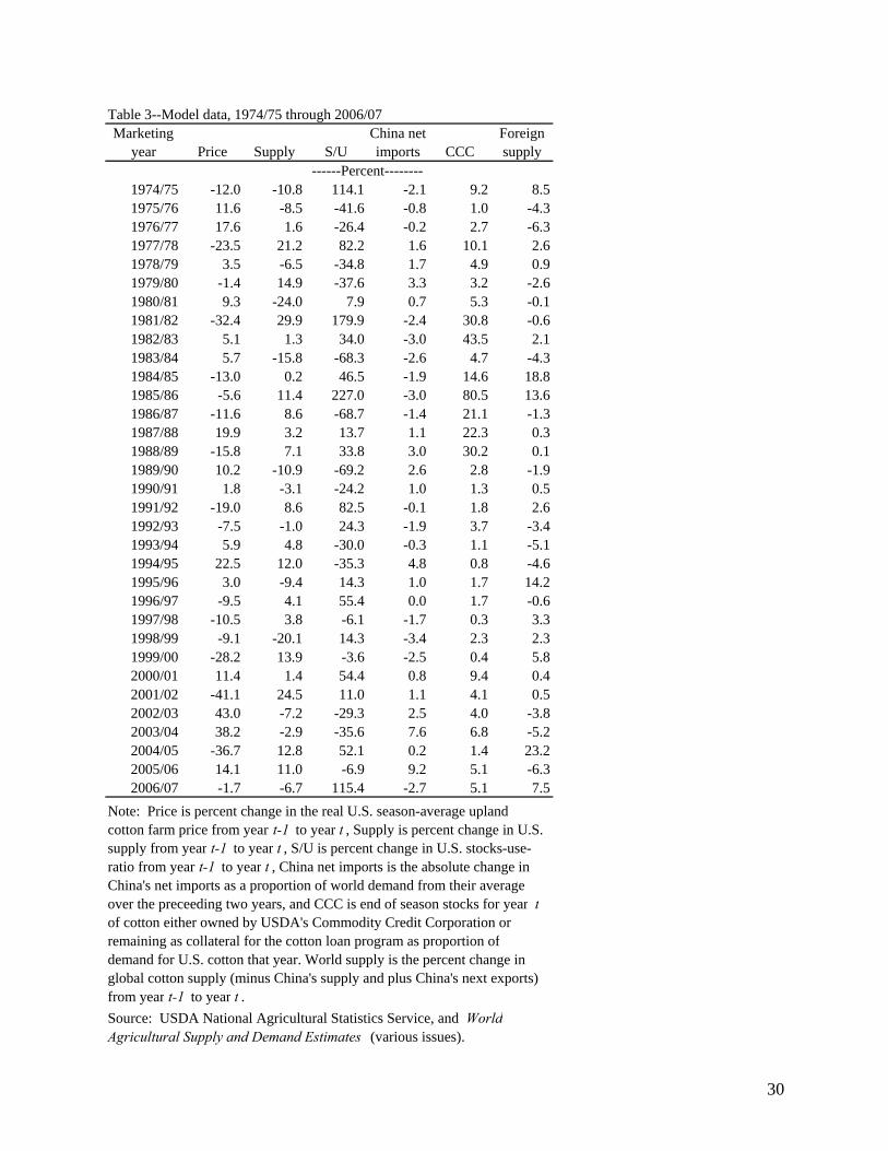
All data used for the empirical estimation of this equation are presented in Table 3. The model is
estimated using the most recently available revisions of supply and demand categories.
Estimation Results
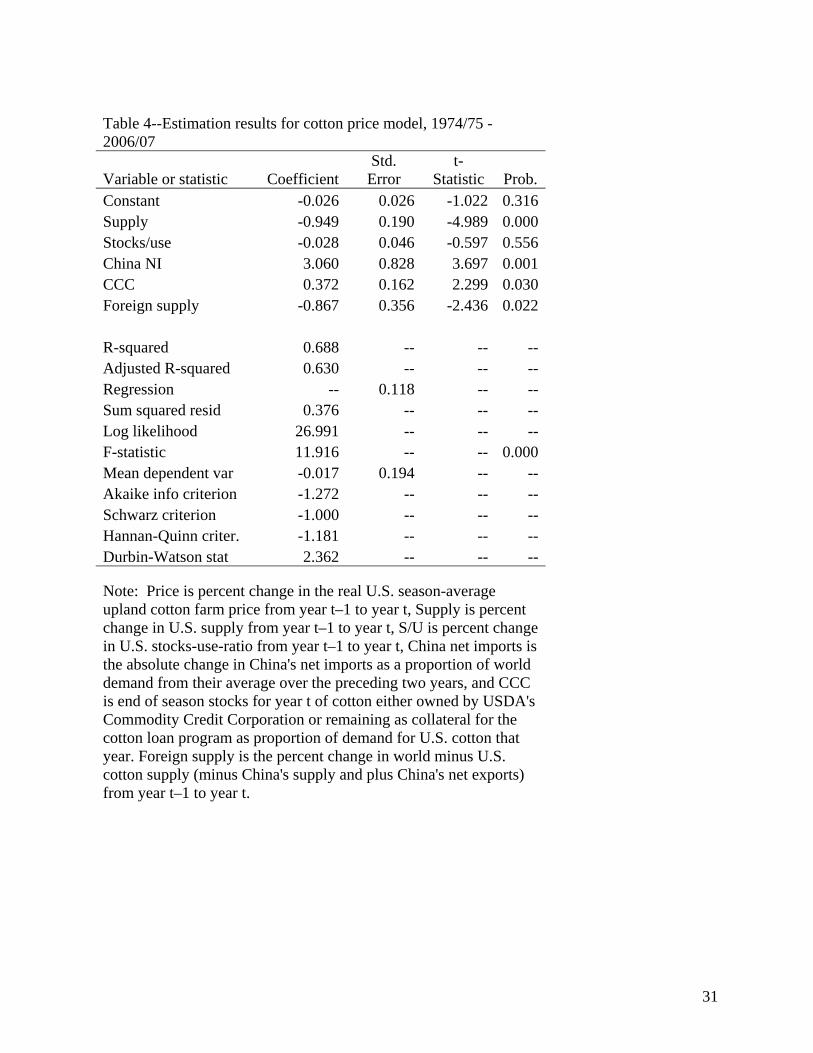
Table 4 presents the results of cotton price model estimation (equation 14) over the
period from 1974/75 through 2006/07. The estimated model explains over 68 percent of the
variation in US upland cotton price. All coefficients except that for the Stocks/Use variable are
significant at the conventional levels and have the expected signs. Since most variables are 7 China’s stocks and production were excluded from this shift variable since the stock data are particularly unreliable (MacDonald, 2007). Stocks were regarded as a state secret in China for many years, and although the degree of secrecy has diminished profoundly even current stock estimates for China are highly conjectural. Production data in China is also considered less reliable than elsewhere, so China’s impact on world supply comes through its net trade position.
16
measured in percent changes, their coefficients are interpreted as elasticities. Thus, a one percent
increase in U.S. Supply from the previous year will cause prices to drop by about 0.7 percent.
The impact of the Stocks/Use variable is not statistically different from zero at the 10 percent
level. A one million bale increase in China NI (net imports) from the average of the previous
two years will cause the U.S. average farm price of upland cotton to increase by 3.1 percent
relative to the previous year’s level. An increase in CCC stocks equal to three percent of U.S.
use would raise price by 0.4 percent. Foreign Supply changes have approximately a one-to-one
inverse effect on price. According to Pearson correlation coefficients presented in table 5,
significant correlation exists between the Stocks/Use variable and several other explanatory
variables in the model. Multicollinearity caused by this variable may inflate standard errors and
R-squared statistic of the model. This issue was investigated by dropping stocks-to-use variable
which resulted in very minor changes (in the second decimal) in the standard errors and the R-
squared and no changes in the signs of the coefficients. Thus it was concluded that
multicollinearity did not cause significant problems in our model.
Note that the low significance of the Stocks/Use variable highlights some differences of
this model from past models, and the changes in world cotton markets. Before adjusting for the
structural change (i.e. estimating equation 12), the parameter for stocks/use is significant at the
12 percent level with the full sample, and if equation 12 is only estimated with data through
1999, the variable is significant at the three percent level. This is despite the presence of
significant collinearity with the CCC variable in this subsample (65 percent correlation). In the
full data set, the Stocks/Use variable is not statistically significant since the United States now
accounts for its smallest share of world production since the early 1800’s and prices are
increasingly set by the supply and demand forces outside the United States.
17
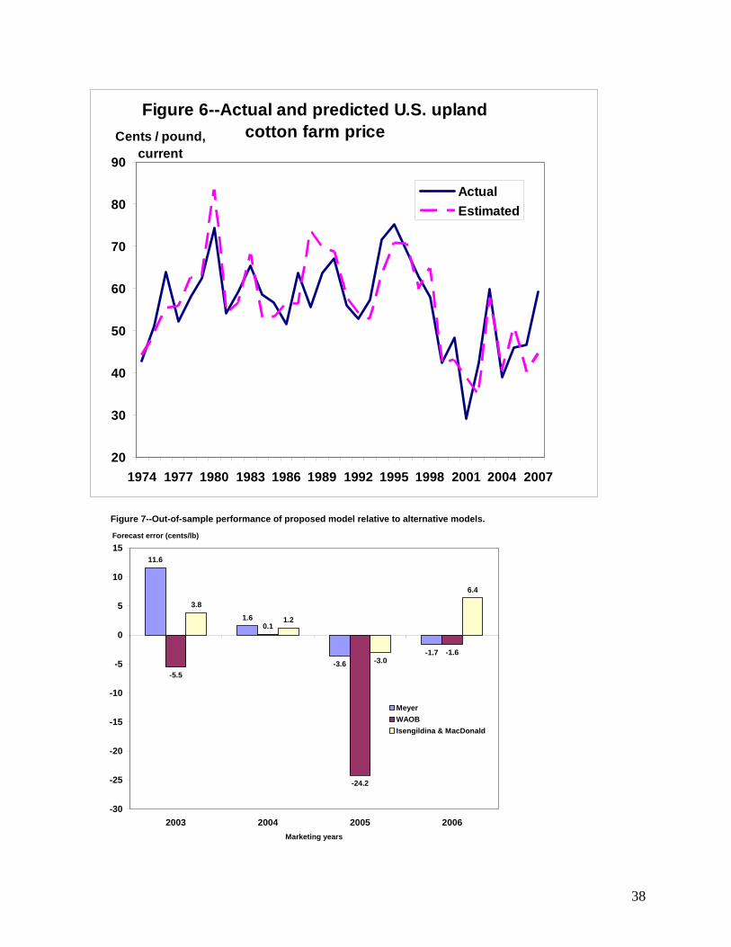
The goodness of fit of the model in nominal prices is illustrated in figure 6. The nominal
prices are calculated by removing inflation adjustment from the real prices predicted by the
model and adjusting them for Step 2 payments. Converting real prices into nominal terms makes
it easier to compare model predictions against the observed prices. Figure 6 demonstrates that
the largest in-sample forecast error of 17.1 cents/lb occurred in 1988. The average forecast error
for the entire sample is 0.2 cents/lb suggesting that the model is unbiased. However, the
importance of these in-sample properties diminishes if the model does not forecast well.
Granger (2005) highlighted that the construction of a model’s evaluation should be
motivated by the model’s purpose. While one purpose of this model is to discern the impact of
supply and demand and policy variables on cotton prices to improve the understanding of these
processes, the primary purpose of the model is to assist forecasting. Jumah and Kunst (2008)
recently demonstrated with a set of grain price forecasting models that statistics assessing in-
sample fit and those evaluating out-of-sample performances can give distinctly different rankings
of model preference. For this exercise, a set of out-of-sample forecasts was calculated by
reestimating the model with a truncated historical sample that ends in 2002/03 and using the
parameters from this truncated sample to estimate subsequent out-of-sample forecasts. Four
years of price forecasts (2003/04 to 2006/07) were calculated using data available in August
2008. Forecast performance was assessed relative to alternative forecasts.
The first alternative is the cotton forecasting model developed by Meyer in 1998.
Meyer’s specification is,
(15) ln(P) = f ( ln(S/U), CHFSTKS, Index, DUMSU, ln(LDP)* DUMSU, ln(1+CCC/Use)),
18
where: CHFSTKS = change in foreign (excluding China) stocks, Index = product of the
September average of the price of the December futures contract and AMS’s September estimate
of the share of expected planted area already forward contracted, DUMSU = dummy valued at 1
when S/U is less than or equal to 22.5 percent, LDP = the difference between the loan rate and
effective loan repayment rate, and CCC = CCC inventory. Thus, the main difference between the
proposed model and Meyer’s model is that Meyer’s model does not take into account changes in
domestic and world supply (which was less relevant during the time that model was developed)
but accounts for the impact of additional information through the index variable connected to
futures prices.
The second alternative is the reduced form model developed by the WAOB in 2006 in an
attempt to reflect the increased export orientation of the US cotton industry. This model’s
specification is,
(16) Pt = f (WxC S/Ut, WxC S/Ut-1, China net exportst),
where: WxC S/U = world excluding China S/U.
The forecast from this model was used as one of the inputs in the USDA’s cotton ICEC forecast.
The biggest difference between the proposed model and the WAOB models is that WAOB
models focuses on international forces, while the proposed model includes the combination of
international and domestic components.
Alternative forecasts have been compared based on their individual mean error to test for
bias, root mean squared error (RMSE) and mean absolute percent error to evaluate the size of the
error, as well as Theil’s U, with comparisons between forecasts based on the Morgan-Granger-
Newbold (MGN) and Diebold-Mariano (DM) statistics (e.g. , Dirion, 2008).
19
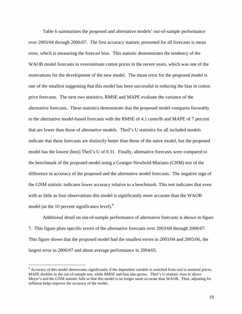
Table 6 summarizes the proposed and alternative models’ out-of-sample performance
over 2003/04 through 2006/07. The first accuracy statistic presented for all forecasts is mean
error, which is measuring the forecast bias. This statistic demonstrates the tendency of the
WAOB model forecasts to overestimate cotton prices in the recent years, which was one of the
motivations for the development of the new model. The mean error for the proposed model is
one of the smallest suggesting that this model has been successful in reducing the bias in cotton
price forecasts. The next two statistics, RMSE and MAPE evaluate the variance of the
alternative forecasts. These statistics demonstrate that the proposed model compares favorably
to the alternative model-based forecasts with the RMSE of 4.1 cents/lb and MAPE of 7 percent
that are lower than those of alternative models. Theil’s U statistics for all included models
indicate that these forecasts are distinctly better than those of the naïve model, but the proposed
model has the lowest (best) Theil’s U of 0.31. Finally, alternative forecasts were compared to
the benchmark of the proposed model using a Granger-Newbold-Mariano (GNM) test of the
difference in accuracy of the proposed and the alternative model forecasts. The negative sign of
the GNM statistic indicates lower accuracy relative to a benchmark. This test indicates that even
with as little as four observations this model is significantly more accurate than the WAOB
model (at the 10 percent significance level).8
Additional detail on out-of-sample performance of alternative forecasts is shown in figure
7. This figure plots specific errors of the alternative forecasts over 2003/04 through 2006/07.
This figure shows that the proposed model had the smallest errors in 2003/04 and 2005/06, the
largest error in 2006/07 and about average performance in 2004/05.
8 Accuracy of this model deteriorates significantly if the dependent variable is switched from real to nominal prices. MAPE doubles in the out-of-sample test, while RMSE and bias also grows. Theil’s U-statistic rises to above Meyer’s and the GNM statistic falls so that this model is no longer more accurate than WAOB. Thus, adjusting for inflation helps improve the accuracy of the model.

20
Another important characteristic for a forecasting model is parameter stability. If
estimated parameters change significantly as new observations are added, the out-of-sample
forecasts may become highly volatile and less accurate, and the model may be misspecified. The
parameter stability features of the proposed model are illustrated in table 7. This table shows
that the parameter estimates are relatively unchanged when estimated using a 1974/75-2002/03
sample versus a 1974/75-2006/07 sample. Furthermore, the out-of-sample forecasts of the model
estimated with the 1974/75-2002/03 sub-sample are only slightly less accurate than the in-sample
estimated prices of the model using the full dataset. This stability bodes well for the model’s
usefulness in future forecasting.
Conclusions and Implications
This study sought to develop a statistical model that reflects current drivers of U.S. upland cotton
prices in response to renewed authority for USDA to publish cotton prices and challenges with
cotton price forecasting reported by various sources in the recent years. A review of the
theoretical framework for commodity price forecasting suggested that changes in supply should
be included in a cotton price model because of the rapid growth in supply due to the spread of
genetically modified varieties and other technologies. Several demand shifters were also
included in a model. China’s net trade as a proportion of world consumption was included to
account for changes in export demand associated with China’s commodity and trade policies.
The impacts of the U.S. farm policy were accounted for by including a variable representing the
amount of cotton in the marketing loan program as a share of domestic consumption and by
adjusting the dependent variable to reflect the impact of the User Marketing Certificate (Step 2)
program.
21
The analysis of cotton price forecasting model identified a structural break that occurred
in U.S. cotton industry in 1999. This structural break was likely caused by a combination of
factors, one of which is an increased export orientation of the US cotton industry caused by the
rapid contraction of the domestic textile industry following the phasing out of the Multifiber
Arrangement (for more information on the end of the MFA, see MacDonald and Vollrath, 2005).
Thus, the proposed model was modified to include the world supply of cotton to reflect the
increased export orientation to correct for the observed structural change. The final model was
subjected to extensive out-of-sample testing to ensure its appropriateness for forecasting.
The out of sample performance measures of the proposed cotton price model suggest that
the model provides a considerable improvement over the naïve forecast. The parameter
estimates and forecast errors do not change much between full sample, and reduced sample used
for out-of-sample forecasting indicating the stability of the model. This stability suggests the
model is an improvement over past forecasting models that have been challenged by the
changing market conditions. Specifically, the out of sample forecasts from the proposed model
are characterized by the lack of bias and relatively low variance. However, the in-sample root
mean squared error of the nominal price predictions projected by this model is 6.0 cents, which is
about 10 percent of the 1974/75-2006/07 average for U.S. upland cotton farm prices. These
errors suggest that there may be some variables omitted from the model.
Omitted variables could include cotton quality characteristics, the role of polyester
(cotton’s primary substitute in textile spinning), the spread of technology like genetically-
modified cotton, and lower transmission of grain price shocks to significant non-U.S. cotton
producers. For example, Olmstead and Rhode (2003) demonstrate that the average staple length
of U.S. cotton rose during the years comprising the historical sample used to estimate this model.
22
The U.S. season-average price is equivalent to the value of the crop of upland cotton divided by
its volume, and staple length is one of the key determinants of the price of a particular bale, or
lot, of cotton. Olmstead and Rhode's data started in 1957, when the U.S. upland crop averaged
32.75 sixteenths of an inch long. In 2006/07 and 2007/08 it averaged 35.3 sixteenths, an increase
since 1957 that in 2007/08 would be worth about 2 cents per pound (Cotton Program, AMS).
However, the impact of these qualitative characteristics on the price of cotton was not included
in this study as it is very difficult to quantify.
Despite non-trivial errors, the proposed model provides useful information particularly in
the environment of highly volatile commodity prices and the increased role of new players in
futures markets. These developments and changing market institutions such as the rise of
electronic trading have raised questions about the relationships among cash prices, futures prices,
and supply and demand fundamentals. Specifically, there has been growing concern about
changes in the relationship between futures prices and cash prices in the United States (Irwin,
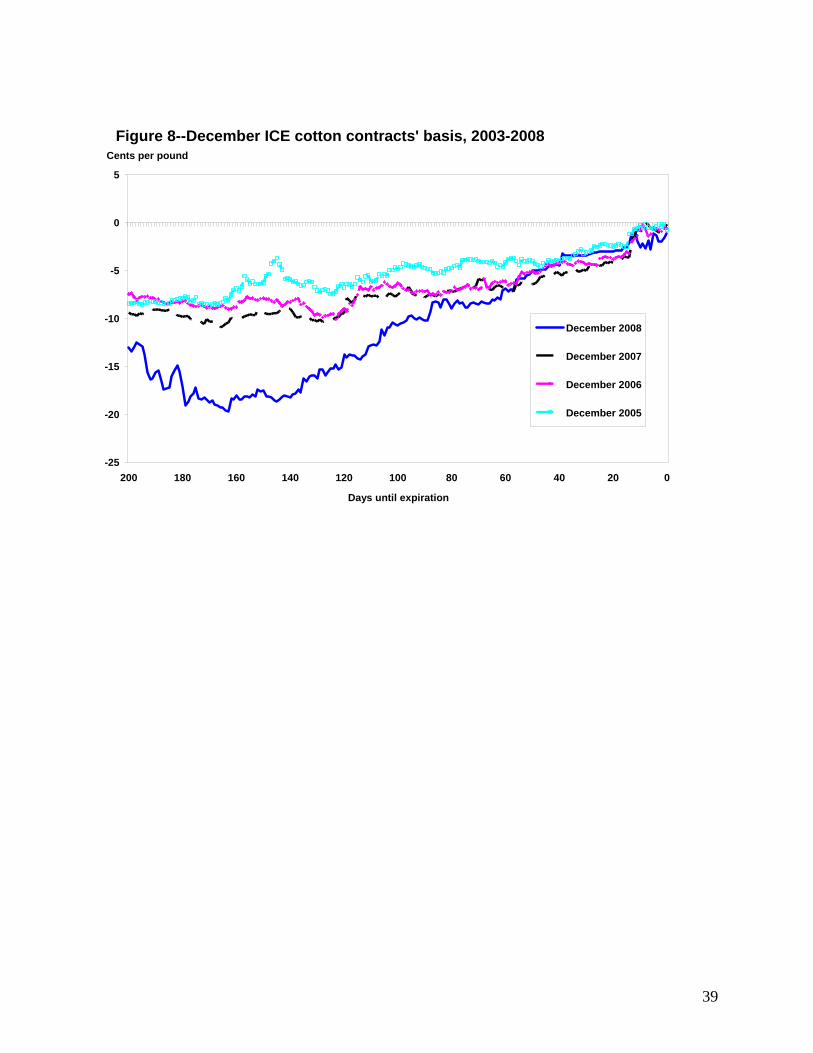
Garcia and Good, 2007). In March 2008, U.S. cotton futures demonstrated nearly
unprecedented volatility. The basis between nearby futures and spot prices remained historically
wide for several months afterward (Figure 6). Therefore, while it would be irrational to ignore
the information provided by futures markets when forecasting the U.S. farm price of cotton, it is
also important to have forecasts that are independent of that information.
The comparison of the out-of-sample performance of the proposed model to that of
alternative models available from other sources revealed that the proposed model relatively
superior to these alternative models. This comparison, however, does not include consensus-
based forecasts that became publically available from the USDA WASDE reports since June
2008. The consensus forecasts were about as accurate as the proposed model, despite the
23
handicap of preliminary supply and demand estimates. The advantage of the consensus
forecasts is the ability to include additional information in the forecasting procedure that is hard
to quantify within the framework of a statistical model. Among other things, this additional
information would include the omitted variables discussed above. The drawback to consensus
forecasts is that they are very specific to current events and difficult to replicate or adjust to
changing circumstances. As such, they are of limited use when presenting policy-makers with
alternative scenarios. A further advantage of model like this one is the opportunity for
consistency-checking. USDA’s ICEC sometimes adjusts its supply and demand outlook in
response to prices, and this model provides an additional tool to aid in that process.
Future avenues for research relate to both world cotton markets and to the characteristics
of USDA’s supply and demand forecasts. While this study correctly identified some aspects of
the structural change that has occurred in U.S. cotton markets since 1999, further examination of
the sources of structural change and the channels through which it affects cotton prices are
needed. In addition, forecasts based on this model will not only depend on the parameters of the
model, but will also be conditional on the forecasts of supply and demand used to derive any
particular forecast of price. Intuitively, early-season forecasts are less reliable than late-season
forecasts, but further research can inform these intuitions, and identify key points in the season
with respect to dynamics of forecast performance within the forecasting season. Furthermore,
the accuracy of specific supply and demand variables and their potential contribution to the
cotton price forecast errors should be examined with the goal of correcting for systematic errors
in these forecasts.
24
References.
Barsky, R.B., and L. Kilian. 2002. “Do We Really Know that Oil Caused the Great Stagflation? A Monetary Alternative.” in NBER Macroeconomics Annual 2001, 16, B.S. Bernanke and K. Rogoff, eds., Cambridge, MA: MIT Press, pp. 137-183. Cotton Program, Cotton Price Statistics Annual Report, Volume 89, No. 13. Agricultural Marketing Service, U.S. Department of Agriculture. 2008 Cotton Program, Cotton Quality Annual Report, Volume 81, No. 8. Agricultural Marketing Service, U.S. Department of Agriculture. 2008 Cotton and Wool Situation and Outlook, Economic Research Service, U.S. Department of Agriculture, November 2001, CWS-2001. Diron, M., (2008), “Short-term forecasts of Euro area real GDP growth: an assessment of real-time performance based on vintage data,” Journal of Forecasting, 27: 371-390. Ferris, J.N., Agricultural Prices and Commodity Market Analysis, WCB McGraw Hill. 1998. Food and Agricultural Policy Research Institute, Impacts of Commodity and Conservation Reserve Program Provisions in House and Senate Reconciliation Bills, FAPRI-UMC Report #15-05, December 2005. Goodwin, B.K., Schnepf, R., and E. Dohlman (2005), Modelling soybean prices in a changing policy environment, Applied Economics, 37: 253-263. Goreux, L., A. Plastina, A. Gruere, and Y. Cao. “The New ICAC Cotton Price Forecasting Model.” Cotton: Review of the World Situation, ICAC, (July-August 2007). Granger , C.W.J. (2005), “Modeling, evaluation, and methodology in the new century,” Economic Inquiry, 43(1): 1-12. Hansen, B.E. “The New Econometrics of Structural Change: Dating Breaks in U.S. Labor Productivity.” Journal of Economic Perspectives 15:117-28. Hansen, B.E. “Approximate Asymptotic P Values for Structural Change Tests.” Journal of Business and Economic Statistics, 15(1)(1997):60-61 Hyndman, R.J., and Koehler, A.B., (2006), “Another look at measures of forecast accuracy,” International Journal of Forecasting, 22: 679-688. International Cotton Advisory Committee, “Where will cotton prices go?,” Cotton Review of the International Situation, 41(3): 3-5. 1988.
25
Irwin, S. H., Garcia, H.H., and Good, D.L., The Performance of Chicago Board of Trade Corn, Soybean, and Wheat Futures Contracts after Recent Changes in Speculative Limits, American Agricultural Economics Association>2007 Annual Meeting, July 29-August 1, 2007, Portland, Oregon Jumah, A., and R.M. Kunst, (2008), “Seasonal production of European Cereal prices: good forecasts using bad models?,” Journal of Forecasting, 27: 391-406. Labys, W.C., Quantitative Models of Commodity Markets, Ballinger Publishing Company, Cambridge, MA 1973. MacDonald, Stephen. “Forecasting World Cotton Prices.” The Ninth Federal Forecasters Conference—Papers and Proceedings,1997, National Center for Educational Statistics, U.S. Department of Education. 1997 MacDonald, Stephen, “Cotton Price Forecasting and Structural Change,” The 15th Federal Forecasters Conference—Papers and Proceedings, 2006 ,Veterans Health Administration, U.S. Department of Veterans Affairs. MacDonald, S., and T. Vollrath, The Forces Shaping World Cotton Consumption After the Multifiber Arrangement, U.S. Department of Agriculture, Economic Research Service, CWS-05C-01, April 2005. Market and Trade Economics Division (2001), Cotton and Wool Situation and Outlook Yearbook, CWS-2001, Economic Research Service, U.S. Department of Agriculture. Meyer, L, S. MacDonald, and R. Skinner. “Cotton and Wool Outlook.” Economic Research Service, U.S. Department of Agriculture, report CWS-08a, March 2008. Meyer, L., MacDonald S., and L. Foreman (2007), Cotton Backgrounder, Outlook Report No. CWS-07B01, Economic Research Service, U.S. Department of Agriculture. Meyer, L.A. “Factors Affecting the US Farm Price of Upland Cotton.” Cotton and Wool Situation and Outlook, CWS-1998, Economic Research Service, U.S. Department of Agriculture, November 1998, pp. 16-22. Mohanty, S., Pan, S., Welch, M., and Ethridge, D., The Impacts of Eliminating the Step 2 Program on the U.S. and World Cotton Market, Briefing Paper CER-BR05-01, Cotton Economics Research Institute, Texas Tech University. 2005. Olmstead, A. L. and Rhode P.W., Hog Round Marketing, Seed Quality, and Government Policy: Institutional Change in U.S. Cotton Production, 1920-1960, Working Paper w9612, National Bureau of Economic Research. 2003.
26
Plato, G., and W. Chambers, (2004). How Does Structural Change in the Global Soybean Market Affect the U.S. Price? OCS-04D-01, Economic Research Service, U.S. Department of Agriculture. Skelly, Carol (2006), unpublished price model in ICEC current supply and demand summary. Skelly, Carol, ICEC Chair, WAOB, private communication, 03/30/2007. Schnepf, R. (2007), “Brazil’s WTO Case Against the U.S. Cotton Program,” CRS Reportfor
Congress, No. RL32571. Stock, J.H., and M.W. Watson. Introduction to Econometrics. Pearson Education, Inc., New
York, 2003. Stultz, H., Glade, E.H., Sanford, S., Lawler, J.V., and Skinner, R.A., Fibers: Background for 1990 Farm Legislation, Agriculture Information Bulletin No. AIB591 Economic Research Service, U.S. Department of Agriculture. 1990 Tomek, W.G., and K.L. Robinson. Agricultural Product Prices. 4th edition. Cornell University Press. 2003. Townsend, Terry P. “This Was a High-Powered Instrument That Sent Its Projectile to the Vitals of the Industry – why USDA Does Not Forecast Cotton Prices.” Proceedings of the Cotton Beltwide Conferences. National Cotton Council. 1989. U.S. Department of Agriculture, Foreign Agricultural Service, Production, Supply, and Distribution Online. http://www.fas.usda.gov/psdonline/ U.S. Department of Agriculture, National Agricultural Statistics Service, Agricultural Prices, September 29, 2008. Wang, D. and W.G. Tomek. “Commodity Prices and Unit Root Tests.” American Journal of Agricultural Economics 89(4)(November 2007): 873-889. Westcott, P.C. Ethanol Expansion in the United States: How Will the Agricultural Sector Adjust? Outlook Report No. (FDS-07D-01) May 2007. Economic Research Service, U.S. Department of Agriculture. Westcott, P.C., and L.A. Hoffman. Price Determination for Corn and Wheat: The Role of Market Factors and Government Programs. Technical Bulletin 1878. Economic Research Service, U.S. Department of Agriculture (1999). Valderrama, C. “Modeling International Cotton Prices.” Proceedings the Cotton Beltwide Conferences. National Cotton Council. 1993.

27
Valderrama, C. “A Revision of the ICAC Price Model.” Cotton: Review of the World Situation, ICAC, 53-6 (July-August 2000). Van Meir, L.W. Relationships among Ending Stocks, Prices, and Loan Rates for Corn. Feed Outlook and Situation Report, FdS-290, Economic Research Service, U.S. Department of Agriculture, 1983.
28
Table 1--Season-ending U.S. commodity program cotton stocks, 1974/75-2006/07.
Marketing year CCC inventory Collateral on outstanding
loans Inventory as share
of use Thous. bales Thous. bales Percent
1974/75 0 235 2 1975/76 0 901 9 1976/77 0 110 1 1977/78 0 309 3 1978/79 1 1209 10 1979/80 0 614 5 1980/81 0 501 3 1981/82 1 626 5 1982/83 396 3643 31 1983/84 158 4267 40 1984/85 124 444 3 1985/86 775 1597 14 1986/87 69 5965 71 1987/88 5 2914 21 1988/89 92 3164 22 1989/90 27 4119 30 1990/91 1 430 3 1991/92 3 215 1 1992/93 13 297 2 1993/94 13 558 4 1994/95 0 179 1 1995/96 0 165 1 1996/97 0 312 2 1997/98 0 311 2 1998/99 6 61 0 1999/00 2 326 2 2000/01 5 68 0 2001/02 108 1460 9 2002/03 97 665 4 2003/04 0 668 3 2004/05 2 1371 7 2005/06 5 301 1 2006/07 51 1185 5
Sources: Stultz et al, Farm Service Agency (FSA) and ERS calcuations based on data from FSA and WASDE.
29
Table 2--Step 2 expenditures and price adjustment variable Marketing year Payments1
Payments/cotton use Subsidy
Adjustment (λt)
Mil.
Dollars dollars/pound Percent Percent 1991/92 140 0.02 2.9 1.6 1992/93 114 0.02 2.7 1.5 1993/94 149 0.02 2.5 1.5 1994/95 88 0.01 1.0 0.6 1995/96 34 0.00 0.5 0.3 1996/97 6 0.00 0.1 0.1 1997/98 416 0.05 6.4 3.7 1998/99 280 0.04 6.7 3.9 1999/00 445 0.05 10.4 6.0 2000/01 236 0.03 5.5 3.2 2001/02 182 0.02 4.9 2.8 2002/03 455 0.05 8.9 5.1 2003/04 363 0.04 5.5 3.1 2004/05 582 0.06 10.7 6.2 2005/06 397 0.04 6.2 3.6
Average 259 0.03 5.0 2.9 1Fiscal year. Sources: Farm Services Agency, and ERS calculations based on data from the Farm Services Agency, WASDE, and Cotlook.
30
Table 3--Model data, 1974/75 through 2006/07Marketing
year Price Supply S/U China net imports CCC
Foreign supply
1974/75 -12.0 -10.8 114.1 -2.1 9.2 8.51975/76 11.6 -8.5 -41.6 -0.8 1.0 -4.31976/77 17.6 1.6 -26.4 -0.2 2.7 -6.31977/78 -23.5 21.2 82.2 1.6 10.1 2.61978/79 3.5 -6.5 -34.8 1.7 4.9 0.91979/80 -1.4 14.9 -37.6 3.3 3.2 -2.61980/81 9.3 -24.0 7.9 0.7 5.3 -0.11981/82 -32.4 29.9 179.9 -2.4 30.8 -0.61982/83 5.1 1.3 34.0 -3.0 43.5 2.11983/84 5.7 -15.8 -68.3 -2.6 4.7 -4.31984/85 -13.0 0.2 46.5 -1.9 14.6 18.81985/86 -5.6 11.4 227.0 -3.0 80.5 13.61986/87 -11.6 8.6 -68.7 -1.4 21.1 -1.31987/88 19.9 3.2 13.7 1.1 22.3 0.31988/89 -15.8 7.1 33.8 3.0 30.2 0.11989/90 10.2 -10.9 -69.2 2.6 2.8 -1.91990/91 1.8 -3.1 -24.2 1.0 1.3 0.51991/92 -19.0 8.6 82.5 -0.1 1.8 2.61992/93 -7.5 -1.0 24.3 -1.9 3.7 -3.41993/94 5.9 4.8 -30.0 -0.3 1.1 -5.11994/95 22.5 12.0 -35.3 4.8 0.8 -4.61995/96 3.0 -9.4 14.3 1.0 1.7 14.21996/97 -9.5 4.1 55.4 0.0 1.7 -0.61997/98 -10.5 3.8 -6.1 -1.7 0.3 3.31998/99 -9.1 -20.1 14.3 -3.4 2.3 2.31999/00 -28.2 13.9 -3.6 -2.5 0.4 5.82000/01 11.4 1.4 54.4 0.8 9.4 0.42001/02 -41.1 24.5 11.0 1.1 4.1 0.52002/03 43.0 -7.2 -29.3 2.5 4.0 -3.82003/04 38.2 -2.9 -35.6 7.6 6.8 -5.22004/05 -36.7 12.8 52.1 0.2 1.4 23.22005/06 14.1 11.0 -6.9 9.2 5.1 -6.32006/07 -1.7 -6.7 115.4 -2.7 5.1 7.5
Note: Price is percent change in the real U.S. season-average upland cotton farm price from year t-1 to year t , Supply is percent change in U.S.supply from year t-1 to year t , S/U is percent change in U.S. stocks-use-ratio from year t-1 to year t , China net imports is the absolute change in China's net imports as a proportion of world demand from their averageover the preceeding two years, and CCC is end of season stocks for year t of cotton either owned by USDA's Commodity Credit Corporation orremaining as collateral for the cotton loan program as proportion ofdemand for U.S. cotton that year. World supply is the percent change in global cotton supply (minus China's supply and plus China's next exports) from year t-1 to year t .Source: USDA National Agricultural Statistics Service, and World Agricultural Supply and Demand Estimates (various issues).
------Percent--------
31
Table 4--Estimation results for cotton price model, 1974/75 - 2006/07
Variable or statistic CoefficientStd.
Error t-
Statistic Prob. Constant -0.026 0.026 -1.022 0.316Supply -0.949 0.190 -4.989 0.000Stocks/use -0.028 0.046 -0.597 0.556China NI 3.060 0.828 3.697 0.001CCC 0.372 0.162 2.299 0.030Foreign supply -0.867 0.356 -2.436 0.022 R-squared 0.688 -- -- -- Adjusted R-squared 0.630 -- -- -- Regression -- 0.118 -- -- Sum squared resid 0.376 -- -- -- Log likelihood 26.991 -- -- -- F-statistic 11.916 -- -- 0.000Mean dependent var -0.017 0.194 -- -- Akaike info criterion -1.272 -- -- -- Schwarz criterion -1.000 -- -- -- Hannan-Quinn criter. -1.181 -- -- -- Durbin-Watson stat 2.362 -- -- --
Note: Price is percent change in the real U.S. season-average upland cotton farm price from year t–1 to year t, Supply is percent change in U.S. supply from year t–1 to year t, S/U is percent change in U.S. stocks-use-ratio from year t–1 to year t, China net imports is the absolute change in China's net imports as a proportion of world demand from their average over the preceding two years, and CCC is end of season stocks for year t of cotton either owned by USDA's Commodity Credit Corporation or remaining as collateral for the cotton loan program as proportion of demand for U.S. cotton that year. Foreign supply is the percent change in world minus U.S. cotton supply (minus China's supply and plus China's net exports) from year t–1 to year t.

32
Table 5--Pearson Correlation Coefficients for Cotton Price Model, 1974/75 - 2006/07.
Supply Stocks/use China NI CCC Foreign Supply
Supply 1.00 0.33 0.13 0.25 0.05 Stocks/use 0.33 1.00 -0.39* 0.60** 0.51** China NI 0.13 -0.39* 1.00 -0.26 -0.39* CCC 0.25 0.60** -0.26 1.00 0.24
Foreign Supply 0.05 0.51** -0.39* 0.24 1.00 Note: Supply is percent change in U.S. supply from year t–1 to year t, S/U is percent change in U.S. stocks-use-ratio from year t–1 to year t, China net imports is the absolute change in China's net imports as a proportion of world demand from their average over the preceding two years, and CCC is end of season stocks for year t of cotton either owned by USDA's Commodity Credit Corporation or remaining as collateral for the cotton loan program as proportion of demand for U.S. cotton that year. Foreign supply is the percent change in world minus U.S. cotton supply (minus China's supply and plus China's net exports) from year t–1 to year t. Number of observations is 33. One asterisk indicates significance at the 5% level (2-tailed), two asterisks indicate significance at the 1% level (2-tailed).

33
Table 6--Evaluation of price forecasting models, 2003/04-2006/071
Model Isengildina and
MacDonald Meyer2 WAOB3 Information set4 2008 2008 2008 Sample 1974-2002 1978-2002 1989-2002 Cents/lb Cents/lb Cents/lb Mean error (bias)5 2.1 2.0 -7.8 Root mean squared error (RMSE) 4.1 6.2 12.4 Percent Percent Percent Mean absolute percent error (MAPE) 7 8 16 Theil's U statistic 0.31 0.39 0.97 Granger-Newbold-Mariano statistic6 -- -0.97 -2.79 Diebold-Mariano statistic7 -- 1.01 0.86
1Model parameters estimated with samples concluding no later than 2002/03. 2Meyer, 1998. 3Unpublished model developed by the World Agricultural Outlook Board. 4Information set used to estimate parameters. For each model, 2008 information is used to determine the values of the independent variables.
5For each year, et = Yt – Ft, where Yt is the actual realization of the price and Ft is the forecast. Therefore, et < 0 is an indication of upward bias. None of the models evaluated here had average forecast means that were significantly different from zero at either the 1%, 5%, or 10% level. 6GNM statistic testing difference between forecast accuracy of Isengildina and MacDonald forecast. None of the differences were significant at either the 1% or 5%. WAOB was significant at the 10% level. 7DM statistic testing difference between forecast accuracy of Isengildina and MacDonald forecast. None of the differences were significant at either the 1%, 5% or 10% level.

34
Table 7--Parameter stability between samples and out-of-sample performance
1974/75-2006/07 1974/76-2002/03 Percent Variable or statistic Coefficient Coefficient Difference Constant -0.026 -0.032 20 Supply -0.949 -0.893 -6 Stocks/use -0.028 -0.041 48 China NI 3.060 3.407 11 CCC 0.372 0.408 10 Foreign supply -0.867 -0.830 -4 Accuracy: 2003/04-2007/08 RMSE 7.221 7.499 4 MAPE 0.120 0.129 -- Theil's U statistic 0.606 0.581 -- Note: Price is percent change in the real U.S. season-average upland cotton farm price from year t–1 to year t, Supply is percent change in U.S. supply from year t–1 to year t, S/U is percent in U.S. stocks-use-ratio from year t–1 to year t, China net imports is the absolute change in China's net imports as a proportion of world demand from their average over the preceding two years, and CCC is end of season stocks for year t of cotton either owned by USDA's Commodity Credit Corporation or remaining as collateral for the cotton loan program as proportion of demand for U.S. cotton that year. World supply is the percent change in global cotton supply (minus China's supply and plus China's next exports) from year t–1 to year t.
35
Figure 1: U.S. season-average farm price, upland cotton
0
20
40
60
80
100
120
140
160
180
1960 1963 1966 1969 1972 1975 1978 1981 1984 1987 1990 1993 1996 1999 2002 2005Source: ERS calcuations based on data from NASS and the U.S. Department of Commerce.
Cents/pound (adjusted to 2000 dollars)
Figure 2--Impact of U.S. consumption subsidy on U.S.
40
45
50
55
60
65
20 21 22 23 24 25 26 27 28 29 30
Million bales
Cents/pound (U.S. price)
SUSD'US
DUS
Source: Simulation of model with linear supply and demand for U.S. and rest of world, substitution between U.S. and ROW cotton, and calibrated to approximate recent realizations of the variables.

36
Figure 3--Impact of U.S. consumption subsidy on ROW
40
45
50
55
60
65
95 96 97 98 99 100 101 102 103 104 105
Million bales
Cents/pound (ROW price)
SROW
DROW
D'ROW
Source: Simulation of model with linear supply and demand for U.S. and rest of world, substitution between U.S. and ROW cotton, and calibrated to approximate recent realizations of the variables.
Figure 4--Quandt Likelihood Ratio Test Results for Cotton Price Model, 1987/88-2006/07
0
1
2
3
4
5
6
1981 1982 1983 1984 1985 1986 1987 1988 1989 1990 1991 1992 1993 1994 1995 1996 1997 1998 1999
QLR statistic
99 percent critical value = 4.12
95 percent critical value = 3.37
90 percent critical value = 3.02

37
Figure 5--U.S. cotton exports and consumption
0
2
4
6
8
10
12
14
16
18
20
1950 1955 1960 1965 1970 1975 1980 1985 1990 1995 2000 2005
Thous. bales
ConsumptionExports
38
Figure 6--Actual and predicted U.S. upland cotton farm price
20
30
40
50
60
70
80
90
1974 1977 1980 1983 1986 1989 1992 1995 1998 2001 2004 2007
Cents / pound, current
ActualEstimated
Figure 7--Out-of-sample performance of proposed model relative to alternative models.
-1.7-3.6
1.6
11.6
-1.6
-24.2
0.1
-5.5
6.4
-3.0
1.2
3.8
-30
-25
-20
-15
-10
-5
0
5
10
15
2003 2004 2005 2006Marketing years
Forecast error (cents/lb)
MeyerWAOBIsengildina & MacDonald
39
Figure 8--December ICE cotton contracts' basis, 2003-2008
-25
-20
-15
-10
-5
0
5
200 180 160 140 120 100 80 60 40 20 0
Days until expiration
Cents per pound
December 2008
December 2007
December 2006
December 2005