Use of odds ratio or relative risk to measure a treatment effect in clinical trials with multiple correlated binary outcomes: data from the NINDS t-PA stroke trial

STATISTICS IN MEDICINEStatist. Med. 2001; 20:1891–1901 (DOI: 10.1002/sim.841)

Use of odds ratio or relative risk to measure a treatment e(ectin clinical trials with multiple correlated binary outcomes:

data from the NINDS t-PA stroke trial

Mei Lu1;∗;† and Barbara C. Tilley2

for theNINDS t-PA STROKE TRIAL STUDY GROUP

1 Department of Biostatistics and Research Epidemiology; Henry Ford Health Sciences Center;One Ford Place – Ste. 3E; Detroit; MI 48202; U.S.A.

2 Department of Biometry and Epidemiology; Medical University of South Carolina; 135 Rutledge Avenue;Post O+ce Box 250551; Charleston; SC 29425; U.S.A.

SUMMARY

In clinical trials, when a single outcome is not su9cient to describe the underlying concept of interest,it may be necessary to compare treatment groups on multiple correlated outcomes. A global test basedon a logit link function provides an estimate of the odds ratio for assessing a common treatment e(ectamong correlated binary outcomes. In this paper we extend the use of generalized estimating equations(GEE) to calculate a common relative risk from correlated binary outcomes based on a log link function.In the context of global tests, we discuss the equivalence and di(erence between logit and log linksand their estimates. We also derive a formula for calculating a common risk di(erence between twotreatment groups based on multiple correlated binary outcomes with categorical covariates, assumingthe asymptotic equivalency between the logit and log-linear links. We discuss the statistical tools tobe used in choosing between the logit and log links when models on di(erent links yield contrastingresults. Examples using data from the NINDS t-PA Stroke Trials are provided. We conclude, in a studyof correlated binary outcomes, that the choice of the logit or log link could be based on a comparisonof goodness-of-link. Copyright ? 2001 John Wiley & Sons, Ltd.

1. INTRODUCTION

Clinical trials may be conducted to study treatment e9cacy in two (treatment and reference)groups using multiple outcomes because no single outcome is su9cient to describe the un-derlying concept of interest. In stroke trials, for example, no single measure of disability

∗Correspondence to: Mei Lu, Department of Biostatistics and Research Epidemiology, Henry Ford Health SciencesCenter, One Ford Place, 3E, Detroit, MI 48202, U.S.A.

† E-mail: [email protected]

Contract=grant sponsor: National Institute of Neurological Disorders and Stroke; contract=grant numbers: N01-NS-02382, N01-NS-02374, N01-NS-02377, N01-NS-02381, N0-NS-02379, N0-NS-02373, N0-NS-02376, N01-NS-02378, N01-NS-02380

Received February 1999Copyright ? 2001 John Wiley & Sons, Ltd. Accepted July 2000

1892 M. LU AND B. C. TILLEY

(for example, Barthel Index, ModiFed Rankin Scale, Glasgow Outcome Scale, or NIH StrokeScale) describes all dimensions of recovery for a stroke patient. Clearly, a treatment compari-son of each outcome at 0.05 level without adjusting for the number of outcomes can increasetype I error [1]. However, the Bonferroni approach, adjusting for the number of outcomes,sometimes can be too conservative [2; 3]. Several global statistics have been developed to testtreatment e9cacy for multiple binary outcomes [2–6]. The listed statistical approaches werebased on a logit link and estimated odds ratios. An odds ratio (OR), the ratio of the oddsof favourable (or unfavourable) responses between two groups, where the odds=p=(1 − p)for some response probability p, can be used to measure an association between treatmentand outcome. Odds ratios have been used extensively in data collected both prospectively (forexample, a cohort study) or retrospectively (for example, a case-control study) when logisticregression is used to adjust for covariates. However, the odds ratio is less commonly used tocommunicate the primary results of a clinical trial because of its lack of clinical interpretation[7]. It measures neither a relative size nor an absolute size di(erence for the treatment e(ecton the outcomes.

As an alternative, the relative risk (RR), unlike the odds ratio, measures the relative sizeof the treatment di(erence, that is, the ratio of the response probability in a treatment groupversus the response probability in a reference group [7; 8]. The relative risk calculated on thebasis of a log link is traditionally used in a prospective study of which randomized clinicaltrials are a special case. For example, in analysing the treatment e(ect on preventing anunfavourable clinical outcome, a relative risk of 0.5 indicates that patients in the treatmentgroup have reduced the chance of having an unfavourable outcome by 50 per cent as comparedto patients in the reference group. From a computational (estimation, iteration and coverage)point of view, the estimate of the odds ratio tends to be more stable than the estimate of therelative risk [9]. The preventable fraction (1-RR), an epidemiologic construct, is the fractionof unfavourable outcomes (cases) in the unexposed (reference) group that could be preventedby the exposure (treatment) group [10]. Prior work in estimating the relative risk was carriedout in situations where a single outcome was considered [11–13]. Wacholder proposed theestimate of relative risk based on likelihood theory using the GLIM algorithm for a singlebinary outcome [9]. He restricted the parameter space by forcing the estimated probability tofall within the interval (0; 1).

A risk di(erence (RD) is the di(erence in response probabilities between two groups, whichis sometimes considered more clinically interpretable than the relative risk because it indicatesan absolute but not relative treatment size di(erence in response probability. It is an intuitivelyappealing measure of treatment e9cacy in clinical trials [14; 7]. The risk di(erence is usefulin that it provides an estimated amount by which a particular response might be increased orreduced if a speciFed treatment is removed [14] and is a particularly important concept whentreatment beneFts are o(set by side-e(ects and=or by a high cost. The reciprocal of the riskdi(erence (1=risk di(erence) indicates the number of patients one needs to treat in order tohave one patient who beneFts from treatment [7]. Usually, the risk di(erence is estimated fora single outcome.

In this paper, we extend Wacholder’s approach to correlated binary outcomes. We usegeneralized estimating equations (GEE), which are developed based on quasi-likelihood theorywith logit and log link functions, for correlated binary outcomes to derive estimates of the oddsratio and relative risk, respectively. Then we discuss the equivalence and di(erence betweenthe two links and their estimates and derive the formula to calculate the risk di(erence for

Copyright ? 2001 John Wiley & Sons, Ltd. Statist. Med. 2001; 20:1891–1901

ODDS RATIO OR RELATIVE RISK TO MEASURE TREATMENT EFFECT 1893

multiple correlated binary outcomes with categorical covariates when models based on the twolinks are asymptotically equivalent. We introduce statistical tools to choose a link functionwhen models on di(erent links give di(erent test results. Finally, we provide examples fromthe two NINDS t-PA Stroke Trials.

2. STATISTICAL BACKGROUND

We consider observations (Yi; Xi), for i = 1; 2; : : : ; N (the number of subjects), where, forthe ith subject, vector Y ′

i =(yi;1; yi;2; : : : ; yi;K) represents K outcomes for some integer K , andX ′i =(xi;1; xi;2; : : : ; xi; q) represents q covariates for some integer q. Suppose Yi has a distribution

of f(·; Ui; �), in which EYi =Ui is a K ×1 vector and � is an unknown scale parameter. Theexpected vector U ′

i =(ui;1; ui;2; : : : ; ui; k) can be expressed as

g(ui; k) = �k + X ′i �

= �k + �1xi;1 + �2xi;2 + · · · + �q−1xi; q−1 + �qxi; q;

for k =1; 2; : : : ; K and i=1; 2; : : : ; N (1)

where g(:) is the link function, �k is the intercept for the kth outcome, �′ =(�1; �2; : : : ; �q−1)are the set of nuisance parameters, and �q is the parameter of interest (for example, thetreatment e(ects) and may depend on k (for example, �q = �q(k)). Assuming the K ×K covariance matrix, Var(Yi)=�V (Ui), for some known K × K matrix V (the workingcovariance matrix), the quasi-likelihood estimator � is the solution of the score-like equationsystem

N∑i=1

(dUi

d�

)′V−1(Ui)(Yi −Ui)=0 (2)

Wedderburn [15] Frst proposed the quasi-likelihood theory. Liang and Zeger [16] developedthe generalized estimating equations (GEE) based on the score-like equations in Equation (2)for multiple or clustered continuous outcomes and for discrete longitudinal data [4]. Prentice[5] later used the GEE approach for correlated binary responses to calculate an odds ratio fora common dose e(ect under the assumption of a common pairwise correlation. However, theGEE algorithm also allows various other correlation structures for binary outcomes beyondthe common pairwise correlation structure.

In Equation (2), � is estimated using a quasi-likelihood function, not a proper likelihoodfunction. To estimate �, we could assume the link function and variance structure withoutattempting to specify the entire distribution of Yi, for i=1; 2; : : : ; N . Equation (2) becomesthe score equation system yielding maximum likelihood estimate of � if matrix V is the truevariance matrix of Yi [17]. Diggle et al. [18] extended this property for the case where thevariance of Yi is a function of the mean. In practice, we often do not understand the detailsof the probability mechanism by which data are generated. Zeger and Liang [4] showed thatthe estimate of � is robust, even under a weak assumption about the actual correlation, bycomparing estimates of � under di(erent correlation structures. This estimation of � using



GEE appears to be more robust than maximum likelihood estimation using GLIM, becausethe quasi-likelihood approach in GEE does not require a fully speciFed underlying distribution.

Equation (2) can be used in conducting a global test for the treatment e(ect on correlatedbinary outcomes assuming a common treatment e(ect on all outcomes (a homogeneous e(ect)or a K-dimensional test for treatment e(ect assuming heterogeneous e(ects. The K-dimensionaltest is more e9cient only when the e(ect of treatment on a single outcome is su9ciently large[19] compared to the global test.

Others have approached the analysis of multiple binary outcomes by combining the multipleoutcomes into a single outcome, sometimes called a composite outcome. As an example,composite outcomes have been used in studying treatments for cardiovascular disease wherea patient who experiences at least one of the events, a myocardial infarction, severe angina ordeath, will be considered as a treatment failure [20; 21]. In stroke studies, we are interested inthe common treatment e(ect among multiple stroke outcomes, and we could create a compositeoutcome from the multiple outcomes where a patient is deFned as a failure if the patient is afailure on any one outcome. The global test has been shown to have greater e9ciency thanthe test of a binary composite outcome (as deFned above) when outcomes are not rare [1]and similar e9ciency when outcomes are rare.

2.1. Models for a common treatment e0ect among multiple binary outcomes

For the remainder of this paper, we restrict ourselves to testing a common treatment ef-fect on correlated binary outcomes. Suppose outcomes Y ′ =(y1; y2; : : : ; yK) are correlatedbinomial responses on N subjects with probabilities of responses P′ =(p1; p2; : : : ; pK) and�1; �2; : : : ; �q−1 is the set of parameters for covariates x1; x2; : : : ; xq−1 other than the treatment.Let �q be the treatment parameter with a common coe9cient for all K outcomes (�q(k)=�q)and xq be an indicator variable with a value of 1 for the treatment group and 0 for thereference group, where q also indicates the total number of covariates in the model, includ-ing the treatment. Equation (1) can be used to describe the probability of response pk on(x1; x2; : : : ; xq−1; xq) with a rather simple form:

g(pk)= �k + �1x1 + �2x2 + · · ·�q−1xq−1 + �qxq (3)

for any k = 1; 2; : : : ; K .Two link functions commonly used in practice are:

(i) the logit or logistic function g(pk)= log( pk1−pk

);(ii) the log link function g(pk)= log(pk), for k =1; 2; : : : ; K .

In addition, let �̂or and �̂rr be the estimates of the treatment coe9cient �q from the logit andlog link models. Based on the logit link and equation (3), we calculate the odds ratio (OR)of the treatment e(ect by taking exp (�̂or). The logit link also Fts Equation (2) so that we candirectly calculate the odds ratio and its 95 per cent conFdence limits under the assumptionsof binomial variance and unspeciFed correlation structure [22].

The log link can be used assuming the count of events obeys a Poisson distribution or whenan estimate of the relative risk is desirable. Using Equation (3), we estimate the treatmente(ect �̂rr and the relative risk, RR =exp(�̂rr). Based on the robustness of the estimation of� as discussed previously, the log link could be a choice in testing for a treatment e(ect oncorrelated binary outcomes although the underlying data may not follow a Poisson distribution.



To estimate the relative risk for multiple binary outcomes assuming a common treatmente(ect, we could use a log link with binomial variance and unspeciFed correlation structure.To achieve convergence, we specify initial values in the expected parameter space for theunknown intercepts, say exp(�k)=0:5 or �k =−0:69 for k =1; 2; : : : ; K . We then calculate thecommon relative risk and its 95 per cent conFdence limits when the iterations converge,without restriction of the parameter spaces. If the algorithm did not converge, di(erent initialpoints would be assigned. From our experience, given a non-negative value of the intercept�k or exp(�k)¿1, for any k =1; 2; : : : ; K , the algorithm always fails to converge. Convergencedoes not appear to depend on the values or signs of the �s.

2.2. Comparison of the logit and log links

If all covariates in Equation (3) are categorical, the log link model simpliFes to the log-linearmodel. Bishop et al. [23] showed the theorem that describes the relationship between Poissonand multinomial estimators. The theorem is described in the following.

Suppose K independent binary responses y1; y2; : : : ; yK are Poisson variates (a log-linearmodel) with parameters m1(�); m2(�); : : : ; mK(�), where � can be single or a vector of param-eters, and y1; y2; : : : ; yK can also be described as multinomial (a logit model) with proportionparameters p1; p2; : : : ; pK , the Poisson maximum likelihood estimate (MLE) equals multino-mial MLE if and only if one of the margins is Fxed. Under this condition, pk has a formpk =mk(�)=

∑Kl=1ml(�), for k =1; 2; : : : ; K .

The clinical trial with a single outcome or independent outcomes could be an applicationof this theorem because the clinical trial could have a predeFned sample size per treatmentgroup that would have a Fxed margin. Under the above conditions, the log-linear model forexpected cell counts could be transformed into a logit model and vice versa.

Another application of this theorem is to derive risk di(erence RD using the parametersfrom both log-linear and logit models with categorical covariates and a Fxed margin. The riskdi(erence has a form

RD=OR − RROR − 1

(1 − 1

RR

)(4)

In addition, we can extend this equivalency to the quasi-likelihood estimation using GEE. Ifthe true variance matrix of Y is based on independent binary outcomes and all covariatesare categorical, we can apply the equivalency directly since the quasi-likelihood estimationbecomes maximum likelihood estimation [17]. Also, we can still assume asymptotic equiva-lency of the logit and log-linear links where the outcomes are correlated because of the weakassumption for the covariance structure [4; 18] required for the quasi-likelihood estimation.RD can be calculated based on OR and RR calculated using GEE. However, RD would notbe exact, but should be close to exact, given weak assumption of covariance.

In practice, the data collected may not always meet the assumption for asymptotic equiv-alency and it may be of interest to include continuous covariates using a log link. Fittedodds ratios in a log model are di(erent from those in the logit model when the model hascontinuous covariate and bivariate responses, illustrated by McCullagh and Nelder [24]. Usingthe quasi-likelihood approach with respect to a not fully speciFed distribution of observations,and a weak assumption of correlation structure, a di(erence in parameter estimates betweenthe logit and log links may exist, but should be less compared to the likelihood approach



which often requires a fully speciFed distribution of observations. Choosing between the logitand the log links sometimes is di9cult. Although the logit model estimating the odds ratioseems to be used more in practice, we should consider the goodness-of-Ft to determine whichlink of the two gives the model with an optimal Ft.

2.2.1. Goodness-of-link in GEE.Commonly, a goodness-of-Ft statistic measures the goodness-of-Ft between observed and

Ftted data generated by a model, which depends on the choice of links, covariates of interestand their coe9cients (the design matrix). Under the conditions that models have the samedesign matrix as described in Equation (3) and are Ft to the same data, but with a di(erentchoice of links, the goodness-of-Ft statistic measures the goodness-of-Ft under the logit or loglink model. Under the latter conditions, we prefer the term goodness-of-link to goodness-of-Ft.

Pearson’s �2 test [25] can be used to assess the goodness-of-link by comparing the goodness-of-Fts for the logit and log links under models with identical design matrices. This teststatistic has been extensively studied and is recommended for the case of a single outcome[26–29], but is not the best choice when there are multiple correlated outcomes [30–32].Holtzman and Good [33] suggested obtaining approximations closer to the exact �2 usingthe moment correction which is described in detail by Read and Cressie [34]. In the GEEalgorithm, the Frst and second moment equations are used in estimating a parameter vector� which contains �k (intercepts) for k =1; 2; : : : ; K , �j for j=1; 2; : : : ; q and parameters inthe working covariance matrix V . Thall and Vail [35] noted that a generalized �2 statisticfrom the expression

∑SiV−1

i Si computed using GEE would be misleading. They propose aquantitative measurement to assess the overdispersion, the primary source of a lack of Ft.Ignoring overdispersion in an analysis can lead to underestimation of the standard errorsof the treatment e(ect and an overstatement of the signiFcance of the treatment e(ect inhypothesis testing. Thall and Vail [35] implemented the statistic H using GEE with the formH =det(var(�̂))−1 for assessing the overdispersion.

Godambe and Heyde [36] have shown that H is an increasing function of the squaredcorrelation coe9cient ( 2) between true � and the estimate �̂. The larger value of log(H)corresponds to a higher coe9cient of 2, hence implying a better Ft to the data. In the GEEalgorithm, although overdispersion is taken into account in parameter estimation, the estimateof log(H) is dependent on the choice of links [4].

3. EXAMPLE FROM THE NINDS t-PA STROKE TRIALS

The NINDS t-PA Stroke Study Group [37] reported on two randomized, double blind, placebo-controlled trials to assess the e(ect of t-PA treatment for patients with an acute ischaemicstroke. A total of 624 patients were enrolled in two separate trials (part I with N =291 andpart II with N =333). The two trials had the same recruitment and data collection protocolbut di(erent primary outcomes. Part I assessed t-PA activity at 24 hours after stroke onset,but three-month data were also collected. Part II was a study of the t-PA treatment e9cacyat 3 months after stroke onset. The primary outcome for part II (a favourable outcome) wasdeFned from four neurological scores at 3 months each dichotomized as success or failure.Success was deFned on the Barthel index (an ordinal scale in increments of 5) as a scoreof 95 or 100, on the modiFed Rankin scale as 0 or 1, on the Glasgow scale as 1, and on



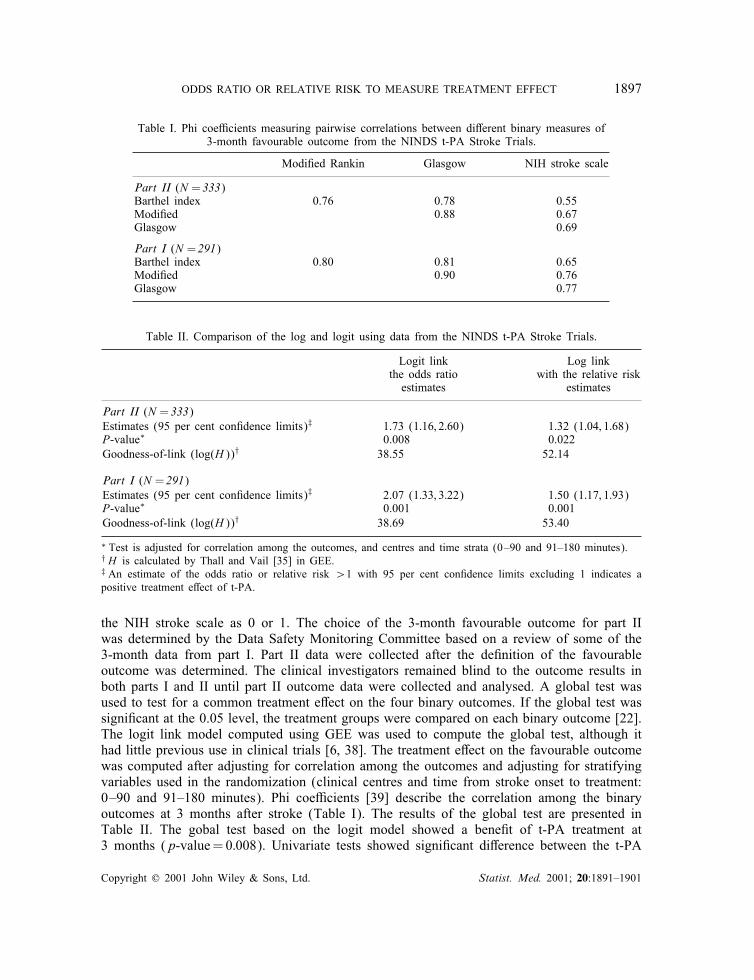
Table I. Phi coe9cients measuring pairwise correlations between di(erent binary measures of3-month favourable outcome from the NINDS t-PA Stroke Trials.

ModiFed Rankin Glasgow NIH stroke scale

Part II (N = 333)Barthel index 0.76 0.78 0.55ModiFed 0.88 0.67Glasgow 0.69

Part I (N = 291)Barthel index 0.80 0.81 0.65ModiFed 0.90 0.76Glasgow 0.77

Table II. Comparison of the log and logit using data from the NINDS t-PA Stroke Trials.

Logit link Log linkthe odds ratio with the relative risk

estimates estimates

Part II (N = 333)Estimates (95 per cent conFdence limits)‡ 1.73 (1:16; 2:60) 1.32 (1:04; 1:68)P-value∗ 0.008 0.022Goodness-of-link (log(H))† 38.55 52.14

Part I (N = 291)Estimates (95 per cent conFdence limits)‡ 2.07 (1:33; 3:22) 1.50 (1:17; 1:93)P-value∗ 0.001 0.001Goodness-of-link (log(H))† 38.69 53.40

∗ Test is adjusted for correlation among the outcomes, and centres and time strata (0–90 and 91–180 minutes).† H is calculated by Thall and Vail [35] in GEE.‡ An estimate of the odds ratio or relative risk ¿1 with 95 per cent conFdence limits excluding 1 indicates apositive treatment e(ect of t-PA.

the NIH stroke scale as 0 or 1. The choice of the 3-month favourable outcome for part IIwas determined by the Data Safety Monitoring Committee based on a review of some of the3-month data from part I. Part II data were collected after the deFnition of the favourableoutcome was determined. The clinical investigators remained blind to the outcome results inboth parts I and II until part II outcome data were collected and analysed. A global test wasused to test for a common treatment e(ect on the four binary outcomes. If the global test wassigniFcant at the 0.05 level, the treatment groups were compared on each binary outcome [22].The logit link model computed using GEE was used to compute the global test, although ithad little previous use in clinical trials [6; 38]. The treatment e(ect on the favourable outcomewas computed after adjusting for correlation among the outcomes and adjusting for stratifyingvariables used in the randomization (clinical centres and time from stroke onset to treatment:0–90 and 91–180 minutes). Phi coe9cients [39] describe the correlation among the binaryoutcomes at 3 months after stroke (Table I). The results of the global test are presented inTable II. The gobal test based on the logit model showed a beneFt of t-PA treatment at3 months (p-value=0:008). Univariate tests showed signiFcant di(erence between the t-PA



Table III. Measuring the association between t-PA and the 3-month favourable outcome – data from theNINDS t-PA Stroke Trials.

t-PA Placebo Risk di(erence Relative Odds%∗ %∗ %∗()† risk† 5% CL‡ ratio† 95% CL‡

Part II: number of patients, N 168 165Barthel index 50 38 12 (13) 1:32 (1:03; 1:68) 1:68 (1:08; 2:62)ModiFed Rankin 39 26 13 (14) 1:45 (1:05; 1:98) 1:81 (1:13; 2:89)Glasgow scale 44 32 12 (13) 1:38 (1:04; 1:82) 1:72 (1:10; 2:70)NIH stroke scale 31 20 11 (13) 1:49 (1:03; 2:17) 1:80 (1:08; 2:99)Adjusted for correlation among outcomesand for the stratifying variables usedin randomization (14) 1:32 (1:04; 1:68) 1:73 (1:16; 2:60)Adjusted for correlation among outcomes only (13) 1:34 (1:05; 1:72) 1:71 (1:15; 2:56)Unadjusted (13) 1:41 (1:09; 1:84) 1:73 (1:15; 2:61)

Part I: number of patients, N 144 147Barthel index 54 39 15 (15) 1:46 (1:13; 1:87) 1:88 (1:17; 3:01)ModiFed Rankin 47 27 20 (20) 1:81 (1:33; 2:47) 2:44 (1:48; 4:02)Glasgow scale 47 31 16 (17) 1:56 (1:17; 2:09) 2:04 (1:25; 3:33)NIH stroke scale 38 21 17 (15) 1:86 (1:28; 2:70) 2:28 (1:34; 3:88)

Adjusted for correlation among outcomesand stratifying variables usedin randomization∗§ (18) 1:50 (1:17; 1:93) 2:07 (1:33; 3:22)Adjusted for correlation among outcomes only (18) 1:44 (1:12; 1:85) 2:06 (1:33; 3:19)Unadjusted (18) 1:56 (1:19; 2:05) 2:10 (1:35; 3:26)

∗ Observed proportions or di(erences in proportions.† Estimates using GEE and equation (4) for calculating the risk di(erence.‡ 95 per cent conFdence limits; for each individual outcome, 95 per cent conFdence limits were adjusted for clinicalcentres and time (0–90 minutes and 91–180 minutes). An estimate of the odds ratio or relative risk ¿1 with 95per cent conFdence limits excluding 1 indicates a positive treatment e(ect of t-PA.∗§ Clinical centres and time (0–90 minutes and 91–180 minutes).

group and the placebo group for each outcome at 0.05 level. Table II also gives the relativerisk based on the log link, again adjusting for the correlation among outcomes and the samecovariates listed previously. Table II also suggests that for these data, the test based on thelog link is more conservative than the test based on the logit link. Although p-values in bothapproaches were less than the critical value of �=0:05, the di(erence in p-values requiresfurther explanation.

To check the goodness-of-link, log(H) was calculated for each link. The log(H) value forthe log link was higher than for the logit link, suggesting that the log link would be a moreappropriate link to test the primary hypothesis in Part II. Similar analyses were performed forPart I with results shown in Tables I and II. Given that the 3-month outcome measure wasderived using Part I data, it is not surprising that the e(ect size in Part II is smaller thanthe e(ect size in Part I. Again, in Part I, the log link yielded a higher log(H) than the logitlink, although the di(erence in p-values appears smaller than for part II. Table III givesthe odds ratios, relative risks and risk di(erences for a favourable outcome comparing thet-PA-treated and placebo-treated groups for Part II and Part I, adjusting for correlation amongoutcomes and the categorical covariates (stratifying variables) described above, adjusting for



correlation among outcomes only, and without adjustment for covariates with the assumptionof independent outcomes. The risk di(erence is similar in all cases (Table III).

In the NINDS t-PA Stroke Trial part II, based on the estimate of relative risk, we wouldconclude that patients treated with t-PA are 32 per cent more likely to have a favourableoutcome compared to the placebo-treated patients (p-value=0:02). Based on the estimate ofrisk di(erence in Part II, we could conclude that for every 100 patients treated with t-PA, 13more patients would have a favourable outcome compared to the 100 patients treated withplacebo. The number needed to treat is estimated as eight, that is, it would be necessary totreat eight patients to observe at least one patient with the favourable outcome.

For illustrating the exact risk di(erence in Equation (4), treatment e(ect on the singleoutcome Rankin as 0 or 1 was calculated without categorical covariates time and clini-cal centres using GEE with estimations of odds ratio 1.79 and relative risk 1.48 based onPart II data. From Equation (4), the risk di(erence is 0.13, which is exactly the same as wehad observed (Table III).

4. CONCLUSION AND DISCUSSION

We have presented an approach using a log link and GEE to compute a relative risk and itsconFdence interval to assess the common dose e(ect for multiple correlated binary outcomes.Relative risk estimation using a log link and GEE based on the quasi-likelihood approachdoes not require a fully speciFed underlying distribution compared to the maximum likelihoodapproach used by other algorithms such as the GLIM algorithm [9].

In practice, the choice of link functions can be determined based on the need for clinicalinterpretation (odds ratio versus relative risk), trial design prior to the data collection, or basedon a comparison of goodness-of-link after reviewing the data. It would be too stringent tohave a complete analysis plan based on a small amount of prior information. We often haveto convince ourselves to choose a non-parametric approach if the normality fails or to choosea dichotomous variable or a transformed variable for a continuous covariate if the linearityfails. A similar scheme should be applied in choosing the link functions. Considering theNINDS t-PA Stroke Trial, if the analysis plan had speciFed a goodness-of-link test to choosethe link function, we would have conducted the global test for the treatment e(ect based onthe log link rather than the logit link. We could then interpret the results using an estimate ofthe relative risk instead of the odds ratio, concluding that patients treated with t-PA are32 per cent more likely to have a favourable outcome compared to the placebo-treatedpatients. However, the same choice of link may not apply to the other trials.

Comparing the results with and without correlation adjustments, a slight reduction in con-Fdence interval lengths is probably due to high correlations. We would expect a greaterreduction in the length of the intervals when correlations among outcomes were decreasedand treatment e(ect did not change the sign among the outcomes. If the treatment is beneF-cial on some of the outcomes and harmful on the others, the length of the interval would beincreased or the global test would be less e9cient [19; 22].

The described approach to the estimation of a risk di(erence is useful in giving descrip-tive summary statistics for the test with multiple outcomes or a single outcome adjusted forcategorical covariates if the two link models are asymptotically equivalent. The consistencyof the risk di(erence estimates across the models in the examples with various covariates or



correlations may be due to either the robustness of parameter estimation in GEE or inherentproperties of the data set. Without conFdence intervals, assessing the impact of the correlationsamong outcomes is di9cult. Future work should include derivation of the variance of the riskdi(erence using the Taylor series expansion approach. It is also of interest to determine theusefulness and interpretation of the risk di(erence when models include continuous covariates.

In conclusion, to study the correlated binary outcomes in a clinical trial, the analysis plan,as speciFed in the protocol, could include an assessment of the goodness-of-link to determinethe link function to be used in the primary analysis.

ACKNOWLEDGEMENTS

This work was supported by grants N01-NS-02382, N01-NS-02374, N01-NS-02377, N01-NS-02381, N0-NS-02379, N0-NS-02373, N0-NS-02376, N01-NS-02378 and N01-NS-02380 from the National Instituteof Neurological Disorders and Stroke, Bethesda, MD.

REFERENCES

1. Lefkopoulou M, Ryan L. Global tests for multiple binary outcomes. Biometrics 1993; 49:975–988.2. O’Brien PC. Procedures for comparing samples with multiple endpoints. Biometrics 1987; 40:1079–1087.3. Pocock SJ, Geller NL, Tsiatis AA. The analysis of multiple endpoints in clinical trials. Biometrics 1987; 43:487–

498.4. Zeger SL, Liang K. Longitudinal data analysis for discrete and continuous outcomes. Biometrics 1986; 42:121–

130.5. Prentice RL. Correlated binary regression with covariates speciFc to each binary observation. Biometrics 1988;44:1033–1048.

6. Lipsitz SR, Laird NM, Harrington DP. Generalized estimation equations for correlated binary data: using theodds as a measure of association. Biometrika 1991; 78:153–160.

7. Sinclair JC, Bracken MB. Clinically useful measures of e(ect in binary analyses of randomized trials. Journalof Clinical Epidemiology 1994; 47:881–889.

8. DerSimonian R, Laird N. Meta-analysis in clinical trials. Controlled Clinical Trials 1986; 7:177–188.9. Wacholder S. Binomial regression in GLIM: estimation risk ratios and risk di(erences. American Journal of

Epidemiology 1986; 123:174–184.10. Miettinen OS. Proportion of disease caused or prevented by a given exposure, trait, or intervention. American

Journal of Epidemiology 1974; 99:325–332.11. Rothman KJ, Boice JD. Epidemiologic Analysis with a Programmable Calculator. NIH Publication No. 79-

1649, US GPO: Washington, DC, 1979.12. Breslow NE. Elementary methods of cohort analysis. International Journal of Epidemiology 1984; 13:112–115.13. Mantel N, Haenszel W. Statistical aspects of the analysis of data from retrospective studies of disease. Journal

of National Cancer Institute 1959; 22:719–748.14. Lilienfeld AM, Lilienfeld DE. Foundations of Epidemiology, 2nd edn. Oxford: New York, 1980.15. Wedderburn RWM. Quasi-likelihood functions, generalized linear models, and the Gauss–Newton method.

Biometrika 1974; 61:439–447.16. Liang K, Zeger SL. Longitudinal data analysis using generalized linear models. Biometrika 1986; 73:13–22.17. Park T. A comparison of the generalized estimating equation approach with the maximum likelihood approach

for repeated measurements. Statistics in Medicine 1993; 12:1723–1732.18. Diggle PJ, Liang K, Zeger SL. Analysis of Longitudinal Data. Oxford University Press: New York, 1994.19. Legler JM, Lefkopoulou M, Ryan L. E9ciency and power of tests for multiple binary outcomes. Journal of

the American Statistical Association 1995; 90:680–693.20. Mentzer RM, Birjiniuk V, Khuri S, Lowe JE, Rahko PS, Weisel RD et al. Adenosine myocardial protection:

preliminary results of a phase II clinical trial. Annals of Surgery 1999; 229:643–649.21. Kaners SD, Banga JD, Stolk RP. Incidence and determinants for mortality and cardiovascular events in diabetes.

Vascular Medicine 1999; 4:67–75.22. Tilley BC, Marler J, Geller NL, Lu M, Legler J, Brott T, Lyden P, Grotta J. Use of a global test for multiple

outcomes in stroke trials with application to the National Institute of Neurological Disorders and Stroke t-PAStroke Trial. Stroke 1996; 27:2136–2142.

23. Bishop YM, Fienberg SE, Holland PW. Discrete Multivariate Analysis: Theory and Practice. The MIT Press:Cambridge, 1975; 447.



24. McCullagh P, Nelder JA. Generalized Linear Models, 2nd edn. Chapman and Hall: New York, 1989.25. Pearson K. On the criterion that a given system of deviations from the probable in the case of a correlated

system of variables is such that it can be reasonably supposed to have arisen from random sampling. PhilosophyMagazine 1900; 50:157–172.

26. Cochran W. The �2 test of goodness of Ft. Annals of Mathematical Statistics 1952; 23:315–345.27. Neyman J. Contribution to the theory of the �2 test. Proceedings of the First Berkeley Symposium on

Mathematical Statistics and Probability 1949; 239–273.28. Watson GS. On chi-square goodness-of-Ft tests for continuous distributions. Journal of the Royal Statistical

Association 1958; 20:44–61.29. Moore DS. Goodness-of-:t Techniques. Marcel Dekker: New York, 1986.30. Tate MW, Hyer LA. Inaccuracy of the �2 test of goodness of Ft when expected frequencies are small. Journal

of the American Statistical Association 1973; 68:836–841.31. Lawley DN. A general method for approximating to the distribution of likelihood ratio criteria. Biometrika

1956; 43:295–303.32. Lawal HB. Tables of percentage points of Pearson’s goodness-of-Ft statistic for use with small expectations.

Applied Statistics 1980; 29:292–298.33. Holtzman G, Good I. The Poisson and chi-squared approximations as compared with the true upper-tail

probability of Pearson’s �2 for equiprobable multinomials. Journal of Statistical Planning and Inference 1986;13:283–295.

34. Read TR, Cressie NAC. Goodness-of-:t Statistics for Discrete Multivariate Data. Springer-Verlag: New York,1988.

35. Thall PF, Vail SC. Some covariance models for longitudinal count data with overdispersion. Biometrics 1990;46:657–671.

36. Godambe VP, Heyde CC. Quasi-likelihood and optimal estimation. International Statistical Review 1987;55:231–244.

37. National Institute of Neurological Disorders and Stroke rt-PA Stroke Study Group. Tissue plasminogen activatorfor acute ischemic stroke. New England Journal of Medicine 1995; 333:1581–1587.

38. Lefkopoulou M, Moore D, Ryan L. The analysis of multiple correlated binary outcomes: application to rodentteratology experiments. Journal of the American Statistical Association 1989; 84:810–815.

39. Kendall M, Stuart A. The Advanced Theory of Statistics, Volume Two. MacMillan Publishing Co: New York,1979.


Documents

Use of odds ratio or relative risk to measure a treatment effect in clinical trials with multiple correlated binary outcomes: data from the NINDS t-PA stroke trial