Embed Size (px)
Citation preview
Use of Technical Condition Indicators as Basis for Residual Useful Life Assessments
Bin Lu
Reliability, Availability, Maintainability and Safety (RAMS)
Supervisor: Jørn Vatn, IPKCo-supervisor: Thor Inge Bernhardsen, Statoil
Department of Production and Quality Engineering
Submission date: June 2014
Norwegian University of Science and Technology


RAMS Reliability, Availability,
Maintainability and Safety
Use of Technical Condition Indicators as Basis for Residual Useful Assessments
Bin Lu
June 2014, Trondheim
Master Thesis
Departement of Production and Quality Engineering
Norwegian University of Science and Technology Responsible Supervisor: Professor Jørn Vatn Supervisor at the company: Thor Inge Bernhardsen


I
Preface
This master thesis is carried out at Department of Production and Quality Engineering, NTNU and is cooperated with the company Statoil. The thesis is a part of education plan in the Master Program RAMS (Reliability, Availability, Maintainability and Safety) Engineering. It is performed during the spring semester of 2014. The topic was put forward in January 2014 by Professor Jørn Vatn. It is extended from the specialization project “Life extension and maintenance optimization in the oil and gas industry”.
The report is written for readers with some background of maintenance engineering and statistical theory. It is also assumed that the reader has a number of knowledge regarding signal processing techniques. Besides, several technical terms are less familiar to readers, hence it is recommended to view technical background in the appendix and consult relevant professional books. Mathematical details could not be interpreted in the thesis due to limits on the page.
Trondheim, 2014-06-10
Bin Lu

II
Acknowledgments
I would like to express my sincere thanks to my supervisor Professor Jørn Vatn at NTNU for guidance as well as the patient teaching and providing me with knowledge about maintenance engineering and statistical models. I also appreciate every other help that were given by Professor Jørn Vatn during my period of study at IPK, NTNU.
Many thanks are also given to my co-supervisor at Statoil, Thor Inge Bernhardsen, for his support and guidance in the project, and comments on the report. I also wish to show my gratitude to Trond Østerås, project manager of ‘Kristin Regularity’, for his patient explanations concerning project details. Besides, I want to thank Harald Rødseth, who provides me sources regarding technical condition indicator.
Finally, I would like to acknowledge my family members and friends. Thank their love, encouragement and support.
B. L.

III
Summary and Conclusions
This thesis is of service to realize residual useful life assessment. Everything in the world deteriorates over time. To know the residual useful life of a piece of equipment contributes to optimal decision-making on its usage time and discards. The rewarding also lies in reduced maintenance cost.
For the application of industry process, a novel approach is proposed to define the term residual useful life, making efforts to satisfy diverse criterion on evaluation of equipment usefulness. In current research findings the definition of residual useful life varies. For maintenance purposes, residual useful life is explained by using diagnostics and prognostics, which are critical elements in condition based maintenance. In the domain of reliability, residual useful life is interpreted with probability theory, where mean residual life and conditional survival probability are frequently utilized.
Rotating equipment is concentrated in which state-of-the-art models and methods for residual useful life assessment are investigated in this thesis. Residual useful life assessment techniques are dependent on deterministic, probabilistic and combined models in representing deterioration behaviors on various types of equipment. Apart from statistical theory, vibration signals, lubrication oil condition and acoustic noise signals are principal elements for the assessment. A stereotyped residual useful life assessment procedure consists of two interdependent stages, off-line deterioration model learning and on-line prognostic model training. In the best of circumstances, the sufficient raw data for the assessment are acquired through run-to-failure tests.
The targeted systems for case study are AC generators and gas turbines served for oil and gas production in Kristin field. Statistical techniques are employed to process and analyze notification data of generators. The regression analysis shows an unimportant relationship between notification date and failure impact. Statistical trend tests do not verify the existence of any monotonic rate of occurrence of failures on AC generators. Vibration data analysis of the gas turbine does not provide monotonic information where residual useful life assessment models could be applied for. The notifications are not demonstrating a systematic pattern. Failures of AC generators and gas turbines are tend to be random. Challenges and recommendations are pointed out for Statoil to execute residual useful life assessment based on current situations. Lubrication oil condition monitoring is strongly recommended in this aspect.
Procedures to realize maintenance optimization are demonstrated as a theoretical case study. Markov state model with inspection and block replacement policy are employed to construct cost models on maintenance optimization. With assumed cost elements, an optimal maintenance program is proposed. The analytic process is practically valuable to verify whether the regular inspection is the optimum maintenance strategy.

IV
Contents Preface ....................................................................................................................... ................. I
Acknowledgments ............................................................................................................... ...... II
Summary and Conclusions ....................................................................................................... III
Nomenclature .................................................................................................................. ......... VI
Chapter 1 Introduction ........................................................................................................ ...... 1
1.1 Background ................................................................................................................ . 1
1.2 Problem Description ................................................................................................... 1
1.3 Objectives ................................................................................................................ ... 2
1.4 Limitations ............................................................................................................... ... 2
1.5 Approach .................................................................................................................. ... 2
1.6 Structure of the Report ............................................................................................... 3
Chapter2 Literature Review .................................................................................................... ... 5
2.1 Overview of Applications on RUL Assessment ............................................................ 5
2.2 Challenges of RUL Assessment ................................................................................... 5
2.3 Terminology ............................................................................................................... . 6
2.3.1 Lifetime ........................................................................................................... 6
2.3.2 Useful Life ........................................................................................................ 7
2.3.3 Residual Useful Life ......................................................................................... 8
2.3.4 Technical Condition Indicator ........................................................................ 13
2.4 State-of-the-art Review on RUL Assessment Methodology ..................................... 14
Chapter 3 A Novel Approach to Define RUL ............................................................................ 16
3.1 Comparison of Various RUL Definitions .................................................................... 16
3.2 A new idea to define RUL .......................................................................................... 17
Chapter 4 RUL Assessment on Rotating Equipment ................................................................ 20
4.1 Rotating Equipment and Major Failure Causes ......................................................... 20
4.2 State-of-the-art Methodological Review on RUL Assessment of Rotating Equipment
.............................................................................................................................. .......... 20
4.2.1 Vibration Signal Analysis for RUL Assessment............................................... 21
4.2.2 Lubrication oil analysis for RUL Assessment ................................................. 24
4.2.3 Nosie Signal Analysis for RUL Assessment .................................................... 24
4.3 Summary and Discussion .......................................................................................... 25
Chapter 5 Case Study - Statistical Analysis .............................................................................. 26
5.1 Statistical Techniques ................................................................................................ 26
V
5.1.1 Counting Process ........................................................................................... 26
5.1.2 Prediction Method-Regression Analysis ....................................................... 27
5.1.3 Trend Test ...................................................................................................... 28
5.2 Statistical Analysis on AC Generators ........................................................................ 29
5.2.1 AC Generator A .............................................................................................. 29
5.2.2 AC Generator B .............................................................................................. 33
5.2.3 Discussions on Analyzed Results ................................................................... 37
5.3 Vibration Trend Analysis on Gas Turbine .................................................................. 37
5.3.1 Gas turbine B ................................................................................................. 37
5.3.2 Use of Overall Vibration Data for RUL Assessment ....................................... 41
5.4 Recommendations for Statoil on RUL Assessment ................................................... 41
Chapter 6 Case Study - Maintenance Optimization ................................................................ 43
6.1 Introduction .............................................................................................................. 43
6.2 Degradation Models ................................................................................................. 43
6.3 Cost Model - Maintenance Optimization .................................................................. 44
6.4 Result Discussion ...................................................................................................... 46
Chapter 7 Summary and Recommendations for Further Work ............................................... 47
7.1 Summary and Conclusions ........................................................................................ 47
7.2 Limitations of Approach ............................................................................................ 49
7.3 Recommendations for Further Work ........................................................................ 49
Appendix A Technical Background ........................................................................................... 50
A.1 Empirical Mode Decomposition (Source: Wikipedia) ............................................... 50
A.2 Paris Law Model (Source: Wikipedia) ....................................................................... 50
A.3 Grey System Theory (Source: Kayacan et al., 2010) ................................................. 50
A.4 Diffusion Process (Source: Wikipedia) ...................................................................... 52
A.5 Nonlinear autoregressive exogenous model (Source: Wikipedia)............................ 52
A.6 Artificial Neural Network (Source: Wikipedia) ......................................................... 52
A.7 Levenberg-Marquardt Algorithm (Source: Wikipedia) ............................................. 52
A.8 ε -Support Vector Regression (Source: Loutas et al., 2013) ................................... 53
A.9 Principal Component Analysis (Source: Wikipedia) .................................................. 53
Appendix B Tables ............................................................................................................. ....... 54
Bibliography .................................................................................................................. ........... 59
Curriculum Vitae .............................................................................................................. ........ 66

VI
Nomenclature
Abbreviation AD Anderson-Darling BRP Block replacement policy
CBM Condition based maintenance CWT Continuous wavelet transform
DFT Discrete Fourier Transform DWT Discrete wavelet transform FFT Fast Fourier Transform
HPP Homogeneous Poisson process MTTF Mean time to failure
NCS Norwegian Continental Shelf NHPP Nonhomogeneous Poisson process OREDA Offshore Reliability Data
O&G Oil and gas PCA Principal Component Analysis PHM Prognostics and health monitoring
PI Statoil condition monitoring system RUL Residual (Remaining) useful life
R&D Research and development RP Renewal process RMS Root mean square
ROCOF Rate of occurrence of failures SAP Statoil Computer-aided Maintenance Management System
SVR Support vectors regression STFT Short-time Fourier Transform TCI Technical condition indicator
WPT Wavelet packet transform WT Wavelet transform Notation
T Lifetime random variable, time to failure of a component or system
t A specific point in time irrespective of global time and local time
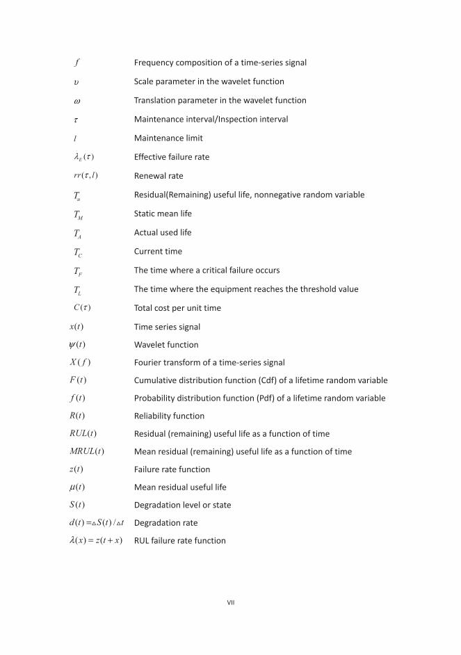
VII
f Frequency composition of a time-series signal
υ Scale parameter in the wavelet function
ω Translation parameter in the wavelet function
τ Maintenance interval/Inspection interval
l Maintenance limit
( )Eλ τ Effective failure rate
( , )rr lτ Renewal rate
uT Residual(Remaining) useful life, nonnegative random variable
MT Static mean life
AT Actual used life
CT Current time
FT The time where a critical failure occurs
LT The time where the equipment reaches the threshold value
( )C τ Total cost per unit time
( )x t Time series signal
( )tψ Wavelet function
( )X f Fourier transform of a time-series signal
( )F t Cumulative distribution function (Cdf) of a lifetime random variable
( )f t Probability distribution function (Pdf) of a lifetime random variable
( )R t Reliability function
( )RUL t Residual (remaining) useful life as a function of time
( )MRUL t Mean residual (remaining) useful life as a function of time
( )z t Failure rate function
( )tμ Mean residual useful life
( )S t Degradation level or state
( ) ( ) /d t S t t= Degradation rate
( ) ( )x z t xλ = + RUL failure rate function

1
Chapter 1 Introduction
This chapter demonstrates the background, problem description, objectives, limitations, approach and the structure of the report for the thesis.
1.1 Background
The oil and gas operators on the Norwegian Continental Shelf (NCS) are facing considerable challenges as facilities are entering the tail-end production phase. Several oil and gas (O&G) facilities were built in the 70’s and 80’s, with a design lifetime typically of 20-30 years, and are now approaching or have reached their design lifetime, see figure 1 (Ersdal et al., 2008). This challenge also applies to operators worldwide due to 30% of more than 6,700 operating platforms have been in operation for more than 20 years (Nabavian et al 2010). With the application of new advanced technology, the recovery factors have been gradually increased over many years, for example from 20 to 50%. The recovery of the oil and gas resources offshore Norway contributes to approximately 25% of Norway’s GNP, 35% of the state income, 20% of all investments and 50% of the export value (Ersdal et al. , 2010). The improvements in extraction technologies as well as high energy prices have led to opportunities for extending the operation beyond the intended lifetime.
Figure 1 Age distribution of existing installations on the NCS (Ersdal et al., 2008)
The effectiveness of O&G industrial performance is determined by the reliability, availability and safety of a system. To ensure that an installation is able to provide sufficient performance on various criteria such as production regularity, safety and maintenance cost it is required to know the technical condition of its parts, components and systems. The residual useful life (RUL) assessment attracts strong interests in industry since it has critical impacts on planning of maintenance activities; spare parts management, functional performance assurance as well as profits obtained from the installation. RUL assessment is also considered to be a critical aspect of aging and life extension management.
1.2 Problem Description
A main challenge when extending the life of an ageing infrastructure or system is to achieve a longer period of economic benefit while ensuring that safety and integrity are maintained. Key factors to consider are the physical deterioration, operation, and

2
maintenance of the system, although less obvious factors may also have an important impact on safety, such as the obsolescence of equipment and changes in the organization. Operating beyond the original design lifetime is known as life extension (LE). Ageing is related to deterioration and may pose a serious risk to the safety of the infrastructure, the personnel, and the environment as the equipment becomes less reliable, obsolete or no longer fit for service, reducing the reliability of safety systems.
The gained knowledge of RUL assessment would lead to the development of cost-effective and lifetime-optimized operation of an installation. The use of technical condition indicators may be one starting point to assess residual useful life (RUL) for these parts, components and systems. For this thesis work, it follows a research and development (R&D) project sponsored by Statoil and executed by SINTEF/NTNU. The contribution from the master thesis as part of the R&D project is shown in chapter 5.
1.3 Objectives
The scope of the master thesis will concentrate on methods, models and approaches to realize RUL assessment. The following objectives will be achieved through the thesis work: 1. Review the literature regarding various use of the term residual useful life as a
basis for giving an explicit definition to be used through the work. 2. Identify two to three classes of critical equipment types as a basis for case studies.
Such classes could be rotating equipment, static equipment and safety systems. 3. For each of the identified classes the literature shall be revived with respect to
which deterministic, probabilistic and combined models are proposed to link technical condition indicators and other degradation measures to residual useful life (RUL).
4. Select one or two cases where models, methods and real condition data could be applied in the aging and life extension management.
5. The case studies shall demonstrate how the maintenance program will affect the technical condition on the equipment, and how to balance maintenance effort with other measures such as upgrading projects, renewal and modification.
1.4 Limitations
The thesis is subject to available methods, models and approaches of dealing with ageing facilities and RUL assessment presented in the literature review and extended work on account of the time limit and complexity. Another limitation lies in available technical and maintenance data supported by Statoil within limited time. Practical RUL assessment is relied on sufficient data and proper prognostics models. Within this thesis, the relatively small amount and few types of real condition data is a major limitation, leading to marginally application of various RUL assessment techniques and RUL estimation models.
1.5 Approach
The main approach of this thesis is based on literature review and discussions with
3
expertise in the project team ‘Kristin Regularity’. The first objective is performed by reviewing the research work that gives the term residual useful life survival. It also contains an extensive review of RUL assessment techniques up to now, by the use of database Engineering Village and Science Direct. Objective two follows the R&D project. The SINTEF project team outlines the production-critical equipment that is analyzed in the thesis. The third objective is achieved by a revived literature review. Objective four considers a specific case study and applies real condition data that is supported by Statoil. The fifth purpose is accomplished by a further work considering an establishment of maintenance program based on the result of RUL assessment.
1.6 Structure of the Report
The thesis mainly consists of three parts. The first part, chapter 2 and 3, is centered on presenting explicit understanding and interpretation of the term RUL. Challenges within RUL assessment are indicated. A terminology study is deduced stating from lifetime, following useful life and residual useful life. The definition and presentation of RUL are based on two main aspects, engineering perspective and statistical perspective. Chapter 2 also gives an introduction on technical condition indicators (TCI). Relevant academic work within TCI research is reviewed. A state-of-the-art review on RUL assessment methodology is included. Chapter 3 compares RUL definitions survived in existing literatures and proposes a new approach to interpret the term.
Part two, chapter 4, identifies critical equipment and revives literature view on relative deterministic, probabilistic and combined models linking degradation measures to RUL assessment. RE is the targeted system. A depth methodological review with RE focused is presented in view of previous literatures in chapter 2. Recent academic contributions within RUL assessment of rotating equipment are investigated and summarized.
The third part performs case studies. Chapter 5 carries out statistical analysis and applies real condition data in the ageing and life extension management. The SAP (Statoil Computer-aided Maintenance Management System) data of AC generators and gas turbines are processed and analyzed, in order to catch their failure tendencies. Chapter 6 proposes the case study on maintenance optimization. Degradation models suitable for a piece of presumed mechanical equipment are constructed where concentrates on deterioration state modelling. Cost models are established based on two distinct maintenance policies.
Chapter 7 gives the summary and conclusion of this thesis. Recommendations for further work are presented in the end.
The preliminary study report and progress report of this thesis are not included in keeping with requirements of the responsible supervisor, Professor Jørn Vatn.

4
Chapter2 Literature Review
To acknowledge the full scope of RUL assessment, it is required to give a clear definition of the term residual useful life. Chapter 2 reviews the literature with respect to various use of the term RUL and gives a distinct definition of RUL used in the thesis. It first starts with an overview of industrial practice on RUL assessment, addressing its practical significance, its role in this thesis and a number of challenges within such field. At the end of this chapter, several explanations used to describe RUL are examined and compared, aiming to rationalize the term residual useful life. The end of this chapter gives an introduction on technical condition indicator.
2.1 Overview of Applications on RUL Assessment
RUL assessment or estimation has received the industry’s great interests recently with environmental, economic and operational purposes. It is regarded as a useful tool in decision-making, specifying current state of the installation and predicting the future remaining life, to decide whether the remaining life of equipment is sufficient for a second life. Great efforts on RUL assessment have been performed in a variety of fields.
As far as I know, the earliest research within RUL assessment is carried out by Watson and Wells (1961), where the work uses mean residual life to study burn-in. In modern industry, RUL assessments are becoming mandatory for economic consideration and assurance of RAMS (Reliability, Availability, Maintainability and Safety) requirements. The aerospace industry predicts the RUL of aircraft critical systems in advance so that effective corrective maintenance can be implemented in time and thereby assures flight safety (Chen et al., 2011). The motivation for RUL assessment in nuclear industry derives from the demand to avoid loss of revenue on condition that unexpected equipment failures will hamper power production of the plant (Shumaker, 2011). In railway domain, RUL assessment is primarily performed as fatigue life evaluation which is addressed in aging management as well as safe transport (Yasniy et al., 2013). The other applications of RUL prediction lie in finance, medicine and weather forecast etc. (Son et al., 2013).
RUL assessment additionally plays a significant role in managing product reuse and recycle. The industries, especially manufacturing and energy domains, are facing a great deal of pressures both from authorities and the public to reduce their industrial wastes. An effective and widely-used strategy is to avoid discarding products and facilities prematurely, which reduces the energy consumption to process raw materials and components. The associated concern will be how to ensure the reliability of used parts without compromising their desired performance. RUL assessment is able to deal with such challenges through estimating the reuse potential of used parts and facilities (Mazhar et al., 2007; Si et al., 2010).
As various areas, the oil and gas industry also requires RUL assessment to be performed on parts, components and systems in order to ensure production regularity, achieve lifetime optimized operation and hereby gain considerable profits.

5
Particularly for offshore industry in the North Sea Norway, the easy oil and gas has been recovered by the large, nevertheless, continuing production is anticipated owing to improved extraction technologies and respectable energy prices. This requires extending the lifetime of production and process facilities since most of them are approaching their design life (Hudson, 2010). Relating to the safety concern in offshore O&G industry, catastrophic failures should be avoided during both normal production and extend-lifetime phase, knowing the RUL facilitate system operators to implement timely maintenance actions for this case.
In this thesis work, the role of RUL assessment is highlighted as a tool to plan necessary maintenance optimally and further eliminate unnecessary maintenance work in aging and life extension management. The practice of RUL assessment is expected to bring benefits to the O&G industry comprising reduced downtime and maintenance cost, optimal management of spare parts together with improved equipment availability.
2.2 Challenges of RUL Assessment
Although extensive work have been done in RUL assessment, it is still difficult to accurately predict the residual useful life under complex operating environments and dynamic loads, particularly with multiple failure modes considered. Operating RUL is dependent on the real conditions of use. The stochasticity, as one of the main characteristics in the system operation, leads to many difficulties and uncertainties in assessing the RUL of equipment, both for deterministic approaches based on failure mechanisms and probabilistic approaches utilizing statistical techniques. As Jin et al. (2013) indicated, uncertainty management is the most challenging aspect of residual life performance prediction.
For complex or large-scale engineering systems, it is typically either cost-expensive or time-consuming to obtain the physical failure mechanisms ahead to capture the physics of failure. The specific failure mechanism knowledge is often hard to gather without interrupting operation. Each engineered system may require creating an entirely new algorithm and model to assess the RUL. The RUL assessment based on failure mechanisms hence has limited ability to transfer from one component to other types of components. Practically deterministic approaches have been realized their inadequacies in tackling the stochastic nature of deterioration process in RUL assessment. On the other hand, the probabilistic approach to assess RUL needs a large quantity of data as well as specialized analysis techniques to process such data. The accuracy is dependent on the quantity and quality of the data and statistical learning techniques. The uncertainties within such approach require rather complex probabilistic tools to handle, particularly taking into account the real operational mode (Si et al., 2013; Maio et al., 2012). To sum up, the recent research in RUL assessment mainly intends to find out solutions for the following questions, which also denote the challenges within RUL assessment:
1. How to develop practical models to describe the residual useful life on various types of equipment concerning the integration of real world dynamical situations?

6
2. For two main approaches to assess RUL of a piece of specific equipment, utilization of deterministic models based on failure mechanism and probabilistic models dependent on distribution of failure records. Which one is promising?
3. Refer to deterministic models, what kind of knowledge is required to adopt such models to assess RUL and correspondingly how to validate their usefulness?
4. Refer to probabilistic models, what kind of data is required to feed these models and how to evaluate the credibility of such models?
5. For industrial application, it may be interested in: How to integrate results of such assessment to the decision-making process? Further, one is perhaps interested in knowing how to standardize or simplify the procedure for RUL assessment?
2.3 Terminology
The result of terminology study on RUL and TCI is shown in this section. A deep and comprehensive understanding of RUL cannot be achieved without a clear cognition of the term lifetime and useful life. The procedure to explain RUL in this section is conducted sequentially starting from the term “lifetime”, followed by “useful life” and ending up with “residual useful life”.
2.3.1 Lifetime
The research of lifetime is extremely widespread through studying length of life of organisms, electronics, structures, materials and devices etc. Normally, it is measured in hours, cycles or in other unit (Finkelstein, 2008). The lifetime in the thesis refers to the time period from the activation time of an item till its end point of service. The lifetime is generally treated as a positive random variable T , characterizing by its distribution function ( )F t . Researchers are interested in knowing the mean life MT in practice, which is obtained by analyzing time-to-failure data of the same type of components under same conditions. For example, the mean life [( 1) / ]MT η β β= Γ + is obtained with using Weibull distribution to model the failure event data of an item (Mazhar et al., 2007). The RUL assessment essentially needs to describe the lifetime in the whole remaining interval of time.
Chakravorti et al. (2013) conceptualized the lifetime of equipment in three ways: physical lifetime, technical lifetime and economic lifetime. Physical Lifetime links to the state where the equipment cannot be used any more in its normal operating state. Technical Lifetime corresponds to the state where the equipment has to be replaced owing to technical reasons even if it can perform its functions physically. Economic Lifetime refers to the situation where the capital value of a piece of equipment depreciates annually.
The technical lifetime links to the case that maintenance of the equipment is exceedingly difficult due to unavailability of spare parts. The economic lifetime relates to the case that operating and maintenance costs may increase over time because of aging and are even beyond the depreciated value of the equipment, indicating the replacement of the equipment is cost-effective (Chakravorti et al., 2013). For a piece of equipment, its technical life or economic life can go to the end

7
even though its physical life left is sufficient to perform the desired performance. The term of life in RUL assessment in this thesis therefore varies to different conditions of the equipment and technical or economic factors that affects the residual useful life of the equipment.
2.3.2 Useful Life
There are a number of definitions with respect to the term useful life. “InvestorWords.com” defines the useful life as “the length of time that a depreciable asset is expected to be usable”, while “Accounting Coach” demonstrates the useful life as “the period of time that will be economically feasible to use an asset.” In “Businessdictionary.com”, the useful life is defined as “the period during which an asset or property is expected to be usable for the purpose it was acquired”. For an industrial system, its useful life is the operating time in which it can perform required functions within the specified performance limits. The useful life perhaps terminates upon a failure or by a determination that the system is no more useful. Figure 2 shows the timeline of the useful life of a system concerning its potential for life extension. At time 0t , the decision regarding life extension has to be taken. The
system’s predicted useful life is 2t .To ensure that the system will not terminate
before 2t , either opportunistic repairs/replacements are required to be planned till
2t or all the crucial replacements are required to be done at 0t (Vaidya and Rausand, 2009).
Figure 2 Timeline of the useful life of a system (Vaidya and Rausand, 2009)
With various definitions, it is evident to see that the key word in the term is “useful” and is difficult to get its uniform definition. Various criterion may be taken to assess whether an asset or equipment is useful or not, for example, depreciation, economic returns and physical condition. To acquire useful life criterion for industrial systems, Vaidya and Rausand (2009) give suggestions to combine expertise from the field of design, manufacturing, safety and system, material degradation, structural integrity, finance and human factors. The research work specifically addresses several criteria to answer if a subsea system will be “useful”: (1) predefined functional requirements, (2) availability, (3) safety and regulatory requirements, (4) environmental requirements, (5) maintenance cost and (6) overall profit margins (Vaidya and Rausand, 2011).
In the bath-tub curve, the useful life is a period of time where an item performs its required functions stably in the normal operating state, typically referring to the normal life period. However, a specific facility perhaps discards even though it is in its normal life period, which is due to undesirable uptime or unavailability of spare parts support. It is more necessary and realistic to consider the value of profits to define the useful life in reality. The useful life in this thesis consequently signifies the period

8
in which a piece of equipment performs its required functions stably meanwhile brings desirable benefits to the owner.
2.3.3 Residual Useful Life
The term of residual useful life is widely-used both theoretically and practicably in operational research, statistics literature, reliability assessment, maintenance optimization and various engineering fields, sometimes named remaining useful life and the acronym RUL is used. Engineers and statisticians give different explanations on this term. From the engineering point of view, RUL is closely associated with physics of an item and failure modes of the equipment. With statistical thinking, the analysis of RUL is established upon probabilistic models and further work in adopting this sort of model to describe residual useful life. In this thesis, the former view corresponds to deterministic models for RUL assessment while the latter view is denoted as probabilistic models. It is expected that the determination of RUL will not be particularly restricted to a specific date and time.
2.3.3.1 Define RUL from engineering perspective
There is no uniform concept survived in the literature review to define RUL in engineering area. The meaning of RUL depends on various context and conditions used in research and study. For instance, Chakravorti et al. (2013) indicated that RUL of transformers is expressed as the service years left to lose the mechanical strength of solid insulation under operational conditions. Yet for carbon filters, its RUL is described as breakthrough times affected by adsorption rate, carbon properties, airflow rate etc. (Mason et al., 2014). Hudson (2010) demonstrates the remnant life of an asset during its life-extended phase, as shown in figure 3. Therein a remnant life assessment is regarded as an estimation of the remaining life by calculating or quantifying the effect of the deterioration mechanisms in comparison with the original design. Failure modes play a significant role in understanding RUL for engineers. It is common to link residual useful life in materials engineering to fatigue life, crack propagation rate and corrosion rate, etc. In mechanical engineering, RUL refers to wear rate. Apart from calendar time, the number of cycles/revolutions is also used in expressing RUL, especially for rotating machinery (Ahmadzadeh & Lundberg, 2013a).
Figure 3
Industrial and maintenance engineers are constantly making efforts to anticipate the

9
failure manifestation and act proactively in order to maximize the equipment’s performance and profits. Recently the modern industry has put considerable attention on implementation of condition based maintenance (CBM), which effectively utilizes knowledge of failure modes to predict RUL of the equipment. CBM is a decision-making strategy to diagnose impending failures, reduce the uncertainty of maintenance activities and foretell the remaining operational life (Peng et al., 2010). It is defined as “predictive maintenance performed as governed by condition monitoring programs” (ISO 13372:2012). Practically condition monitoring data, such as vibration data and oil analysis data, are collected and processed to decide future equipment health condition and further to predict its RUL (Tian et al., 2011). The reliability and maintenance cost are main criterion frequently adopted by maintenance engineers to schedule maintenance work in reality. Figure 4 shows the relationship between RUL and such two criterions. RUL denotes as time to failure. When it reaches zero, the system will break down, correspondingly, the maintenance cost increases significantly and the reliability of the system decreases. It needs to be emphasized that knowledge on the failure propagation process and failure mechanisms are important in an effective CBM program (Peng et al., 2010). In the view of maintenance engineering, the understanding of RUL is closely related with diagnostics and prognostics which are two significant aspects of CBM.
Figure 4
Diagnostics is defined as “examination of symptoms and syndromes to determine the nature of faults or failures (kind, situation, extent)” by ISO 13372:2012. Its main task is to detect, isolate and identify faults when abnormity occurs. It shows whether the monitored system indicates something wrong, locates the faulty item and determines the nature of the fault. Although diagnostics do not address direct information on RUL assessment, it provides the operator reports on whether a specific failure is present or not, particularly when failure prediction of prognostics fails and a failure occurs RUL estimation is more likely a prior event analysis in analogy to prognostics but not a posterior event analysis as diagnostics (Jardine et al., 2006)..
In comparison with diagnostics, the term prognostic is used more frequently in relation with RUL. RUL estimation is regarded as one of the most critical components in prognostics and health management (PHM) (Si et al., 2013). The objective of prognostics is to predict the RUL (Ahmadzadeh and Lundberg, 2013a). ISO 13372:2012 defines prognostics as “analysis of the symptoms of faults to predict future condition and residual life within design parameters”. Similarly, ISO 13381-1:2004 defines prognosis as a “technical process resulting in determination of remaining useful life”. IEEE Reliability Society gives a relative definition combining

10
PHM as “a system engineering discipline focusing on detection, prediction and management of the health and status of complex engineered systems” (Ma, 2009). Farrar and Lieven (2006) describe damage prognosis as “the estimate of an engineered system’s remaining useful life”.
Prognostics are usually effective for faults and failure modes with known, age-related, or progressive deterioration characteristics (ISO 13381-1:2004). It uses automated methods to detect, diagnose, and analyze the degradation of physical system performance, calculating the acceptable remaining life before the occurrence of unacceptable degraded performance (Peng et al., 2010). Predicting the residual useful life of an item is a main concern of prognostics, as Jardine et al. (2006) pointed out, the most widely used prognosis is to predict the time left before the occurrence of a failure given the current machine condition and past operation profile. Therein the time left before failure observation usually refers as RUL.
The end of this section reviews how an engineer gives response when he is asked about RUL. In the engineer’s opinion, RUL is the operating time left on equipment before it is down for required major maintenance. Some RUL is dependent on Vendor recommendations, some are based on experience, and the others are counted on deterministic analyses. The majority of them are dependent on experience. In the operation, remaining life and risk of failure are both useful to be predicted. A number of maintenance actions are based on RUL while others are relied on current condition. The engineer stressed that RUL turns out to be critical when failure modes are known or predictable within scheduling maintenance. In the event of unpredictable failures and randomly changing conditions, the RUL becomes meaningless in planning maintenance (Banjevic, 2009).
2.3.3.2 Define RUL from statistical perspective:
Compared to engineers, researchers in the field of statistics, operation and reliability analysis generally talk about life models, economic models and replacement policies (Ahmadzadeh & Lundberg, 2013a). The residual useful life of a component or system is typically demonstrated as the length from the current time to the end of its useful life, expressed as a nonnegative random variable uT . A simple and concise way to
acquire uT is through achieving the period between the static mean life MT and
the dynamic actual used life AT (Mazhar et al., 2007). According to Rausand & Høyland (2004), Finkelstein (2008), Nystad (2008), Banjevic (2009) and Ahmadzadeh & Lundberg (2013a), the following part of this section is deduced to define residual useful life for non-repairable and repairable items separately in the perspective of a reliability analyst or a statistician. This part is carried out in a general way and not refers to a specified industrial system. The end of this section further gives an application case, which demonstrates RUL of an industrial system from statistical perspective, namely RUL in a subsea context.
RUL for non-repairable items
Non-repairable items are generally discarded by the first failure. For an item of age t , consider the nonnegative lifetime random variable T , representing random time to

11
failure of this unit. Let ( ) Pr( ), 0R t T t t= > ≥ , be its reliability function. T is assumed to be absolutely continuous for simplicity. Its existing probability density function (Pdf) is denoted as ( )f t and its cumulative distribution function (Cdf) as ( )F t :
0Pr( ) 1 Pr( ) 1 ( ) ( ) , 0,
( )0, 0.
tT t T t R t f u du t
F tt
≤ = − > = − = ≥=
>
0 0
( ) ( ) Pr( )( ) ( ) lim limt t
d F t t F t t T t tf t F tdt t t→ →
+ − < ≤ += = =
( )F t denotes the probability that the item fails within the time interval (0, ]t and a maintenance action is required to be performed. The failure rate function ( )z t of the item is obtained:
0 0
Pr( ) ( ) ( ) 1 ( )( ) lim lim( ) ( )t t
t T t t T t F t t F t f tz tt t R t R t→ →
< ≤ + > + −= = =
Extending from the statement above, the residual useful life ( ) uRUL t T T t= = − (whenT t> ), is used to describe the remaining time to failure beyond the age t , see figure 5. Let ( ) ( ) ( ), 0u u uR x P T x P T t x T t x= > = − > > ≥ be its reliability
function, ( )( ) ( )( )
u
u
f xx z t xR x
λ = = + be RUL failure rate function,
( )( ) ( ) ( )( )u u
f t xf x z t x R xR t
+= = + be RUL probability density function and
( ) 1 ( ) 1 ( ) 1 ( )u u u uF x R x P T x P T t x T t= − = − > = − − > > be RUL cumulative distribution function. Further, mean residual useful life (MRUL) is defined as
0 0
( )( ) ( ) ( ) ( )
( )t t
u
R x dxt E T t T t R x dx R x t dx
R tμ
∞∞
= − ≥ = = = , where ( )R x t is the
conditional survival function of an item that has survived till the age t .
Figure 5
RUL for repairable items
Repairable items are able to perform the desired functions after the implementation of proper maintenance actions. They are typically not discarded by the first failure. The end service time for them may be determined by high maintenance cost or unavailability of maintenance support.
Consider a repairable item that is put into operation at time 0t = . 1S denotes the

12
time of first required maintenance action. It is assumed that the repair action is perfect which is able to bring the failed item back to the functioning state. It is further assumed that the repair time is neglected. A sequence of required maintenance action times 1 2, ...S S will be obtained. Let iT be the interoccurrence time for 1, 2...i = and ( )N t be the integer number of maintenance actions in the time interval (0, t]. iS refers to the global time while iT indicates the local time, hence
1 2 ...i iS T T T= + + + . { ( ), 0}N t t ≥ is called a counting process. It can be represented
by the sequence of maintenance action times 1 2, ...S S or by the sequence of
interoccorrence times 1 2, ...T T . The most popular stochastic point processes used to model repairable systems are homogeneous Poisson process (HPP), renewal process (RP), and nonhomogeneous Poisson process (NHPP). The RUL corresponds to the period between an arbitrary point in time t (a specific point in time irrespective of global time and local time) and the time to next required maintenance action. For instance, if we stand at time 't and intend to know the RUL of the item, its RUL can
be described as '3S t− , see figure 6.
Figure 6
RUL in a subsea context
The research work to define RUL within a subsea context is performed by Vaidya and Rausand (2009; 2011) from a statistical view. The technical health, future operating conditions and future environmental conditions are decided as main factors influencing RUL of a subsea system: (1) 1TH denotes the technical health of the
system at time 1t , see figure 7. It corresponds to the knowledge (K) about the
equipment up to time 1t . The survivor function 1 1( , ( ), )R t t TH t K expresses the
relation between the technical health and the reliability of the equipment. (2) 1( )O t describes expected operational conditions and planned interventions that are predicted at time 1t , estimating the operating condition that would prevail from 1t till the end life of the item. The estimation relies on the experience and expert judgment. (3) 1( )E t expresses the expected environmental conditions that may
prevail after time 1t . uT is used to measure the time from 1t until the system is no
longer useful. The distribution of uT relies on the technical health 1TH at time 1t , the expected operational conditions ( )O t and the expected environmental

13
conditions ( )E t . The probability distribution function of uT at 1t is achieved to be
1 1 1 1( ) Pr[ , ( ), ( )]u uF t t T t TH O t E t= ≤ .
Figure 7
2.3.4 Technical Condition Indicator
Technical condition can be viewed as a static value. It affects the residual useful life of a component or system, particularly for cases when operators change the operating conditions of equipment (Thorstensen, 2007). A simple example could be: the residual useful life of an engine shaft may increase or decrease in case the external stresses are reducing or increasing. Through the literature review, the main contribution to use technical condition indicator for estimating RUL lies in Thorstensen (2007), Nystad (2008) and Vaiyad & Rausand (2009, 2011).
The technical condition of an item at time t in Vaiyad & Rausand (2009, 2011)’s research is defined as the status or perform ability of the item as measured by a set of indicators at, or immediately before time t . A number of indicators either continuously measurable or discrete are needed to tell the status of the item, such as vibration, oil level, speed etc. The technical condition of an item at time t is denoted as 1 2( ) ( ( ), ( ),... ( ))kx t x t x t x t= with k different indicators measured. It is regarded as a measurement (sensor readings) and no assessment is contained.
In the Thorstensen (2007) and Nystad (2008)’s research, technical condition indicator refers to technical condition index. It is a measure developed in the EUREKA project “Ageing Management (1996-1999) (www.eureka.be)”, as part of the Norwegian Research Council founded program PROSMAT 2000. The purpose of this project is to develop a new and reliable variable, technical condition index, which is only affected by the change of the system’s technical integrity. The following definition is used:
The Technical Condition Index, denoted TCI, is defined as the degree of degradation relative to the design condition. It may take values between a maximum and a minimum value, where the maximum value describes the design condition and the minimum value describes the state of total degradation.
Early alerts will be available in case problems are developing by using TCIs and the organization can take necessary actions. Compared to traditional indicators, for instance, regularity, accident statistics and environmental emissions, TCI has a high sensitivity with respect to technical condition. The evaluation of technical condition is related to five principal contexts: safety, environment, availability, man-hours and costs (Nystad, 2008).
Thorstensen (2007) presents a model developed to examine and obtain optimal solutions when it is possible to classify the present technical condition of the items and predict the residual life. The thesis work uses a Markov model to describe the deterioration process, where the sequential decision problem is modelled as a

14
discrete time Semi-Markov Decision Process. An offshore gas turbine is worked on as a cases study. Nystad (2008)’s research utilizes aggregated TCI paths to estimate the RUL of natural gas export compressors. The technical condition determination methods are derived from the TeCoMan software. TeCoMan possessed by Marintek is a program developed to calculate the TCI as well as other types of KPI’s. It is supported with a range of different aggregation methods and functions to transfer measurement readings to a unified indicator (TeCoMan Wiki).
As reviewed from Nystad (2008)’s project work, the RUL assessment only uses reliability as the single criteria to evaluate the usefulness of the equipment, which may not be so appealing on condition that maintenance cost, spare parts availability etc. are considered in reality. Integrating information obtained from RUL estimation to decision-making in maintenance planning is the most important aspect which gives the assessment process meaningful. The lack of incorporating maintenance issues in RUL assessment may weaken the producing practical significance. Another limitation is related to the real condition data required to feed TeCoMan program and reliability models. The uncertainty management in the RUL assessment is not performed in the research, which reduces the accuracy of the estimation. The assumption of perfect inspection in Thorstensen (2007)’s thesis is quite limited in reality.
2.4 State-of-the-art Review on RUL Assessment Methodology
RUL assessment comprises two aspects. One is related to RUL estimation, namely systematic use of information to predict or calculate RUL, depending on specific contexts, either to achieve a numerical value or the probability of surviving a particular period of time, or simply a classification of degradation states. The other is to describe the process of judging the tolerability, the goodness etc. of the results from RUL estimation/analysis. The former finds the ‘values’ of RUL and the latter compare it with relevant requirements, such as RAMS requirements (Lecture note: TPK5170). RUL estimation is the core part of assessment procedure. The sequential comparison of estimation results with requirements generally appeals for an establishment of maintenance program for a piece of equipment in case its estimated RUL does not fulfill the expectation.
This section summarizes and compares current RUL estimation methods used both in the theoretical and practical work. The deterministic models based on physics of failure and probabilistic models relied on statistical techniques are two separate approaches to carry out RUL estimation, where the hybrid of such two methods also survive in the research. The review watches the probabilistic model closely in view of that no specific equipment is focused and no background information from the industry is provided.
Table B. 1 (page 54) summarizes the state-of-the-art review on various RUL estimation methodologies presented by different authors. The review is performed through using the database ‘Engineering Village’ and limited to the accessibility to

15
full texts. Most relevant and recent papers are recorded while non-relevant and outdated papers are neglected. The literature investigation shows that prognostic models are widely-adopted to perform RUL estimation through using given condition and health monitoring information (Ahmadzadeh & Lundberg, 2013a; Son et al., 2013; Si et al., 2012). Figure 8 demonstrates the taxonomy of different approaches for RUL estimation. The techniques can be broadly classified as physics-based, experimental, data-driven and hybrid approaches, where experience based approach is not addressed. The comparison of these methods is presented in table B. 2 (page 59).
Physics based methodology typically builds theoretical models to demonstrate the physics of the system and relative failure modes, for instance, fatigue crack growth, corrosion and wear. Experimental based methodology uses experiments to collect essential raw data to achieve a better understanding of the life time of components. The studies include, for example, energy engineering, engineering materials and chemical processing. Even though scientists and researchers in such fields do not use the terminology RUL, actually the experiments are designed for this purpose. Differ from the two methods above, the data-driven methodology does not require specific knowledge about products, but depends on the utilization of condition monitoring data to estimate RUL, where generally expects a large quantity of data to be available. Hybrid methodology indicates using two or more prediction methods in conjunction to improve the accuracy of RUL estimation (Ahmadzadeh & Lundberg, 2013a; Son et al., 2013; Si et al., 2012).
In this thesis, physics based methodology refers to the utilization of deterministic models for RUL estimation. The data driven methodology corresponds to the adoption of probabilistic models for this purpose. The hybrid approach uses several different methods to estimate RUL. Experiment-based approach is not addressed since it closely relates to specific engineering domains and requires experiments.
Figure 8

16
Chapter 3 A Novel Approach to Define RUL
Chapter 3 gives a novel approach to define RUL. The term has various definitions with different interpretation aspects based on review work. As a key measure of using RUL to realize maintenance optimization, the new way to define RUL considers maintenance issues as main target. Practically evaluating the usefulness of equipment may become complex and difficult. Many efforts are required and expected.
3.1 Comparison of Various RUL Definitions
The engineering perspective to define RUL is based on knowledge of engineering principles, physics of failure and underlying failure mechanisms. In this domain, engineers are required to possess professional knowledge on various deterioration mechanisms, for instance fatigue, corrosion, embrittlement, erosion and mechanical wear. The level of expert comprehension decides the accuracy of RUL estimation. Generally there is a number of failure mechanisms associated with one specified failure mode. The dominant failure mechanism takes the leading part in assessing RUL of equipment. It is therefore not necessary to analyze all failure mechanisms but competing ones to identify the dominant failure mechanism that limits the length of RUL (Vaidya and Rausand, 2011).
A useful tool to identify the different failure modes in a hierarchical structure is Failure Modes, Effects & Criticality Analysis (Rausand and Høyland, 2004). In industrial and maintenance engineering, RUL assessment needs to consider monitored condition monitoring information, operational, performance, environmental information and degradation signals. Bespoke condition monitoring equipment are required to be installed to provide such information, such as vibration, oil condition, temperature, humidity, pressure, speed, loading etc. (Si et al., 2011).
The statistical view to define RUL only considers a component or system’s physical condition without counting on any physics or engineering principle. Its fundamental issue is to find the probability density function (PDF) of the RUL. Estimating the RUL is then realized by evaluating the conditional lifetime distribution given that a system has survived up to a specified time, for instance T t T t− > , where T signifies the lifetime. The obtained RUL distributions generally depend on the life characteristics of a population of identical systems and available lifetime data (Si et al., 2013). The available statistical data determines the accuracy and authenticity of RUL assessment. This point of view to define RUL properly applies to the situation where the relative reliability function can be obtained, for example, in case the degradation life of an item is described as a Weibull distribution, then the corresponding Pdf and Cdf is known, further ( )MRUL t can be obtained.

17
Through the literature review, it is hard to arrive that whether the engineering thinking to define RUL is more accurate or the statistical perspective to describe RUL is more appropriate. Both of them have their own characteristics. The engineering view requires professional knowledge on material degradation, equipment operation etc. Generally speaking, knowing the dominant reason why the equipment fails obviously contributes to better understanding its RUL survival length (Vaidya and Rausand, 2011). The statistical view requires lifetime data to express the RUL. Si et al. (2013) pointed out that such data are in short supply in reality or even non-existent at all for systems that are costly or time-consuming to collect. An exact and closed-form of the RUL distribution is perhaps only available for some special cases. The real situation in defining RUL is normally restricted to the knowledge of equipment possessed by operators and available data that can be used to feed RUL estimation models. A hybrid approach to treat RUL assessment both dependent on engineering thinking and statistical techniques is expected to be more realistic and make up their own shortages.
The literature review indicates that the most fundamental challenge to define RUL in industry still lies in which criterion is used to answer whether one component or system is “useful” or not. The criterion differs to various duty holders and operating environments. A starting point to define RUL should demonstrate how the term “useful” means to the operator and what level of performance is anticipated on the equipment. In case various criteria exist, the optimal ones can be decided through utilizing multi-objective optimization methods.
3.2 A new idea to define RUL
Considering multiple criteria used to evaluate the usefulness of equipment
Differ from the conventional illustrations of RUL in the field of engineering and statistics, a new way to demonstrate the RUL refers to the remaining time period of a piece of equipment in where realize its anticipated performance and is able to bring desirable profits to the owner. The criteria used to evaluate whether the performance is desired or not, meanwhile to decide the threshold value shown in figure 9, may vary due to different operation surroundings and various duty holders.
Table 1
Criteria used to evaluate the performance of equipment Output quality Output quantity Reliability Availability Maintainability Safety/Risk Overall equipment effectiveness Logistics Inventory of spare parts Personnel management Environmental impact Technical support Deprecation cost Operation cost Maintenance costs(discounted) Maintenance quality
Table 1 gives a generic list of criteria for this concern. The owner can define the required criterion to determine the point of time where the residual useful life ends,

18
namely the time reaching the limit of threshold value. The RUL is then more likely an economical quantity, taking various criterions into account. Compared with traditional probabilistic approach to assess RUL through using reliability as unique criterion, the utilization of various criteria for RUL assessment will make it more widespread and practically appealing.
Figure 9
As shown in figure 9, the threshold value may be derived from one of the criterion listed in table 1, or a vector of several ones. A better practice of setting this value can be achieved by considering engineering experience, the analysis of past data and the recommended standards. The date LT for the equipment to reach the threshold
value is assumed to be prior to the time FT where critical failure occurs, otherwise such thinking is meaningful less. RUL is then determined by the period between the current time CT and the time in which the equipment reaches the limit value,
namely RUL= L CT T− . Correspondingly, the residual useful life is equal to F CT T− .
The degradation progression curve is required to be established prior to determination of RUL. ( )S t denotes the degradation level or state. Degradation rate is then equal to ( ) ( ) /d t S t t= . The assessment of degradation rate requires degradation models as well as data of measured historical degradation rate and influencing factors.
The critical failure indicates a failure where brings huge damage to the equipment, or even personnel injury and disasters. A direct and convenient way to determine the critical failure time is through lifetime modeling. The second method to decide the critical failure could be through using deterministic models based on failure mechanisms. With proper treatment, the external triggering events, such as shock, are also able to be included in this illustration.
In case reliability is selected as the single criteria, the traditional statistical way to define RUL is sufficient for the assessment process. With this view, RUL assessment equals to residual lifetime assessment. On condition that other criterions are considered, for instance, safety and operation cost, it needs novel approaches, perhaps relevant economic models, to integrate such input parameters to the RUL assessment procedure.

19
Chapter 4 RUL Assessment on Rotating
Equipment
Chapter 4 starts to perform RUL assessments for critical type of equipment. The determination of critical equipment follows the project “Kristin Regularity”. Kristin is located in the southwestern part of the Norwegian Sea, 16 km south west of the Åsgard field. It has been developed with twelve production wells in four subsea templates tied back to a semi-submersible platform. Kristin produces about 10 million cubic meters of gas per day. Production capacity is 125,000 barrels of condensate and more than 18 million cubic meters of rich gas (www.statoil.com).
The analysis of data derived from SAP indicates that the gas export system contributes the largest to production loss, and the maintenance cost of main power systems is the highest. Based on study and discussion with expertise in the project team, the rotating equipment is determined as the first type of critical equipment for RUL assessment. This chapter starts with the study of major failure causes of rotating equipment, following a state-of-the-art overview of most-relevant RUL assessment methods.
In view of supported background information and already acquired maintenance data from Statoil, RUL assessment will mainly takes reliability as criteria to evaluate the usefulness of concerned equipment, meaning that the length of RUL ends at the point of time when a critical failure occurs. In other words, the majority of RUL assessment work equals to prediction of residual lifetime for specific equipment. The novel definition of RUL given in chapter 3 requires various types of data for relevant assessment work, for instance operation cost and depreciation cost, consequently the innovative approach to estimate RUL is not able to be developed due to lack of required data.
4.1 Rotating Equipment and Major Failure Causes
Rotating equipment are equipment that moves liquids, solids or gases through a system of drivers, driven components, transmission devices and auxiliary equipment, which is used to add Kinetic energy to a process. It is mainly classified as four types on the basis of different functions (Forsthoffer, 2005), see table 2.
Table 2 Driven equipment
Drivers-prime movers
Transmission devices Auxiliary equipment
Compressors Steam turbines Gears Lube and seal systems Pumps Gas turbines Clutches Buffer gas systems Extruders Motors Couplings Cooling systems Mixers Engines Fans

20
Like other types of equipment, rotating equipment does not fail without a cause. A comprehensive understanding of major failure causes of rotating equipment contributes to better forecasting machinery failures as well as predicting the RUL. Certainly, there are a number of factors required to be considered in RUL assessment for rotating machinery, for instance, original design, manufacturing tolerance, assembly, working environment, load nature and maintenance work. Particularly taking the design philosophy into consideration, the interaction between applied forces on rotating equipment under normal condition will lead to a stable operation with minimum noise and vibration. The loss of equilibrium force as a result leads to further fault enhancement (Da Costa et al., 2010). Noise and vibration signals therefore provide distinct measurements on degradation status of rotating equipment.
As a specialist providing rotating machinery consulting service to the O&G industry over 40 years, Forsthoffer (2005) points out that the root cause of rotating machinery failure lies in the supporting auxiliary system. A persistent inspection of auxiliary equipment condition, such as temperature and lubrication oil level, is recommended even during component replacement. OREDA handbook (2009) gives a list on failure modes of gas turbines operating in the North Sea: abnormal instrument reading, breakdown, external leakage-fuel, external leakage-utility medium, erratic output, fail to start on demand, high output, internal leakage, low output, noise, overheating, parameter deviation, minor in-service problems, structural deficiency, fail to stop on demand, spurious stop and vibration. Therein noise and vibration is specially focused in the thesis, intending to relate such failure modes to RUL estimation. Other failure modes, for instance leakage and output issues, are not addressed due to inadequate techniques for relating them to RUL estimation.
4.2 State-of-the-art Methodological Review on RUL Assessment of Rotating Equipment
The existing methods to estimate RUL of rotating equipment can be grouped into three main categories: (1) Reliability approaches-event data based estimation; (2) Prognostics approaches-condition monitoring data based estimation; and (3) Hybrid approaches-estimation based on both event and condition monitoring data (Heng et al., 2009; Gebraeel et al., 2009; Sikorska et al., 2013). An overview of utilizing various methods to estimate the RUL of rotating machinery can draw on relevant articles listed in table B. 1 (page 54), article number: 4, 6, 10, 15, 17, 18, 22, 24, 30, 33, 35, 36, 43, 44, 45 and 47. The review shows that recent RUL assessment research is mainly rotating-machinery-concerned, taking bearings for instance. Provided sufficient information and data, both physics based and data-driven RUL estimation methods are able to achieve the desired assessment purpose.
Generally, reliability approaches to estimate RUL are dependent on the distribution of failure event records of a population of identical units. Machine reliability is modelled through using parametric failure models, for instance Exponential, Weibull and Lognormal, where a number of them are elaborated in most reliability-focused

21
books, like Rausand and Høyland (2004). This type of estimation is greatly useful to manufacturers since high volumes of units are available to be taken as analysis sample, but is less valuable to end users, for instance, mean-time-to-failure of a whole population cannot attract interests of a maintenance engineer yet the ongoing reliability information of a specific component or system does (Heng et al., 2009; Gebraeel et al., 2009; Sikorska et al., 2013). This approach does not consider multiple types of failure modes as well as dynamics of operating conditions and environments, which limits its application in RUL assessment on rotating equipment working in Kristin field.
Compared to reliability methods, prognostics approach and hybrid approaches is much more promising in estimating RUL of rotating machinery (Heng et al., 2009; Gebraeel et al., 2009; Sikorska et al., 2013). The defects caused by imbalance, misalignment, bearing faults and lubrication faults all lead to variation of rotation of the equipment. Therein the vibration inspection is widely adopted as diagnosis methods to describe the deterioration process of rotating machinery (Goto et al., 2008). An example could be predicting the RUL of rotating machinery through sampling the acoustic signal over its lifetime. Scanlon et al. (2013) argues that the acoustic noise signal contains sufficient information to effectively predict the RUL of rotating equipment, illustrating by a case study where the used rotating machine has several moving parts, including two rotating element bearings.
The following section demonstrates how to link vibration, noise signal and lubrication oil condition to RUL estimation, with focus on vibration. The purpose is to demonstrate most recent research work in this area and establish a solid foundation for further determination of proper method utilized in case study considering real condition data.
4.2.1 Vibration Signal Analysis for RUL Assessment
There has been an increasing strong interest to indicate the health of rotating equipment through the analysis of vibration signature, normally frequencies and magnitudes (Atoui et al., 2013). The vibration signal is not a direct source of information and its effectiveness in RUL assessment depends on available signal processing techniques.
Fourier Transform
The Fourier Transform is a traditional approach for vibration signal analysis, particularly with the consideration of stationary signals. It exposes the frequency feature of a time series ( )x t through transforming it from the time domain into the frequency domain, hence generating the spectrum ( )X f that includes the entire signal’s fundamental and its harmonics (Al-Badour et al., 2011). One of its definition
is given by Gao and Yan (2011): 2( ) ( ) i ftX f x t e dtπ∞ −
−∞= , where ( )x t is the
time-series signal and f denotes the frequency composition. Afterwards, the Fourier Transform is extended to the fast Fourier transform (FFT)-based order analysis (OA) technique, discrete Fourier Transform (DFT) and short time Fourier Transform (STFT) in the particular field of vibrations and machinery health

22
monitoring, allowing for an effective tracking of speed-driven harmonics of rotating equipment. Although FFT is widely used in signal processing, whereas it has no ability to demonstrate the time dependency of the spectrum of analyzed signal, which limits its application in dealing with non-stationary signals. It is recommended to employ FFT to process stationary signals (Al-Badour et al., 2011).
Wavelet Transform
Wavelet transform (WT) is an effective tool to process non-stationary signals and extract the signal’s time domain (Loutas et al., 2013). AI-Badour et al. (2011) point out that the utilization of wavelet transform is able to present a local signal analysis or zoom on concerned time intervals whereas keep the spectral information intact. This tool is particularly significant for applications on damage (crack) or fault detections.
Mathematically, a wavelet is a square integral function ( )tψ which satisfies2( )
( )fdf
f∞
−∞
Ψ< ∞ , where ( )fΨ is the Fourier transform (i.e. frequency domain) of
the wavelet function ( )tψ (time domain). Its continuous version, the continuous
wavelet transform (CWT), is defined as *1( , ) ( ) ( )twt x t dtωυ ω ψυυ
∞
−∞
−= , where
*( )ψ ⋅ is the complex conjugate of the scaled (parameter υ ) and translated (parameter ω ) wavelet function ( )ψ ⋅ . The practical signal processing normally employs the discrete wavelet transform (DWF), since performing the CWT will lead to the problem of redundant information. The DWF can be achieved by discretizing the scale parameter υ and translation parameter ω , until get the satisfied signal mapping. Another major wavelet transform is wavelet packet transform (WPT). It is an attractive tool to detect and differentiate transient elements with high-frequency
features. The wavelet packet is defined as
( ) ( )2
( ) ( )2 1
( ) 2 ( ) (2 )
( ) 2 ( ) (2 ).
j jn n
k
j jn n
k
u t h k u t k
u t g k u t k+
= −
= − with
0,1, 2,...n = and 0,1,...,k m= , where (0)0 ( )u t is the scaling function ( )tφ and (0)
1 ( )u t is the base wavelet function ( )tψ . The superscript ( )j signifies the j th level wavelet packet basis. There will be 2 j wavelet packet bases at the j th level (Al-Badour et al., 2011; Gao and Yan, 2011).
Loutas et al. (2013) perform the latest RUL assessment work through using wavelet transform technique combined with data-driven probabilistic ε -Support Vectors Regression (SVR) (Article No. 46 in table B.1, page 54). The gradual degradation of rolling bearings is considered and their features are extracted from the acceleration waveforms. Several run-to-failure experiments in bearings under various loading conditions are carried out with two vibration sensors mounted on the bearings for the monitoring of degradation phenomena. The threshold value is decided as a failure criterion in the test, namely an indicator of critical fault, and the RUL therefore ends in case the critical fault occurs. The tests are stopped when the vibration root

23
mean square (RMS) acceleration hit the threshold. Both FFT and WPT are employed to acquire the most monotonic behavior during the test, which is chosen as inputs to the SVR model (Appendix A Technical Background). The established probabilistic SVR model is used to predict the RUL of rolling element bearings.
Goto et al. (2012) execute another RUL assessment work based on vibration signal analysis (Article No. 37 in table B. 1, page 54Table B. 1). The RUL evaluation is verified by actual data collected from rotating equipment in thermal power plants. The velocity and acceleration of vibration are state variables to indicate the deterioration of rotating equipment, refers to as the deterioration management values, meaning that if the deterioration management value is beyond a threshold value, a repair or replacement is required. RUL in this research therefore ends when the deterioration management value reaches the threshold value. Special acceleration sensors are used to map the amplitude of vibration acceleration and velocity for rotating equipment. Figure 10 shows the conceptual diagram of RUL estimation based on the prediction of the deterioration management value. The deterioration management value for velocity is 1 2( )v n v n vy t c t c= + and for acceleration is 2 1( ) exp( )a n a a ny t c c t= ,
where nt is the n th measurement of time and 1 2 1, ,v v ac c c and 2ac are parameters of the model. The model parameters are estimated through using the exponentially weighted recursive least squares approach. ( ), 1,...,n my t m l+ =
denotes the predicted deterioration management value, where nt is the current
time. ( )n my t + is calculated by 1( ) ( ) ( ) ( ), 1,...,v n m v n v n n m v ny t d t c t t y t m l+ += + − = for
velocity and 2 1( ) ( ) ( )exp( ( ) ) ( ) 1,...,a n m a n a n a n n m a ny t d t c t c t t y t m l+ += + − = for acceleration.
Figure 10
The predicted deterioration management value ( )i n my t + at time n mt + is calculated by using the deterioration model. The standard deviation of the prediction errors
( ) ( ) ( )i n m i n m i n me t y t d t+ + += − of the deterioration management values are used to
evaluate the confidence interval of the predicted value, where ( )i n md t + is the
actual deterioration management value at time n mt + . ( )n me t + are assumed to be
independently and identically distributed as 2(0, ( ))i n mN tσ + where
2
1
1( ) { ( ) ( )} , , ,1
nn k
i n m i k m i k mnk
t y t d t i v aρσ ρρ
−+ + +
=
−= − =−
1,...,m l= . Then the residual

24
useful life *m of the rotating equipment is evaluated by *
( 1,2,...,arg{ min { ( ) ( ) , , }}i n m i n m im l
m y t r t i v aσ λ+ +== + > = . In case the upper value of the
confidence interval ( ) ( ), ,i n m i n my t r t i v aσ+ ++ = is beyond a threshold value iλ , it
appeals for maintenance intervention, where iλ can be prior determined by expert judgment.
4.2.2 Lubrication oil analysis for RUL Assessment
Lubrication oil analysis plays a critical role in detecting gas turbine failures as well as in condition-based maintenance. The availability of a functioning turbine is mainly dependent on the protective performance of the lubrication oil for its transmission parts (Zhu et al, 2013). Poley (2012) claims that condition monitoring of lubrication oil delivers roughly 10 times earlier warnings for machine failures compared to vibration based monitoring techniques. Zhu et al. (2013) carry out the recent research work within this domain (Article No. 6 in table B. 1, page 54). Particle filter technique is utilized to estimate the RUL of the lubrication oil depending on the viscosity or dielectric constant sensor observations. An l -step ahead estimator is established to give a long term prediction of the state pdf ( )k l kp x Z+ of oil condition, for 1,...,l T k= − , where T is time of failure. An unbiased l -step ahead
estimator is 1
11
( ) ... ( ) ( )k l k l
k l k j j k k jj k j k
p x Z p x x p x Z dx+ + −
+ −= + =
= ∏ ∏ , where the state t kx =
denotes the particle contamination level at current time k . RUL is the object’s remaining usable time before it needs maintenance or fails. For instance, let .thrλ represents a pre-specified threshold value for the state of oil condition, the object’s RUL at time k is computed as ( )kRUL k l k l= + − = given t k lx = + is beyond .thrλ . With the determination of .thrλ , the estimation of RUL l≤ is equal to the estimation of .k l thrx λ+ ≥ , which is .Pr( ) Pr( )k k l thr kRUL l Z X Zλ+≤ = ≥ (Zhu et al., 2013).
The implementation of particle filter technique for RUL assessment requires a physical model that relates the water contamination level and temperature to the dielectric constant and kinematic viscosity.
4.2.3 Nosie Signal Analysis for RUL Assessment
Noise signal from rotating machinery contains essential information about the internal process and is capable of providing valuable information for RUL assessment. Kavanagh et al. (2008) argues that sound intensity and sound pressure that explains the mechanism of noise generation contributes to distinguish the good from the bad bearings with spectral analysis and statistical analysis. Scanlon & Bergin (2007) and Kavanagh et al. (2008) employ the analysis of acoustic noise signal to predict the RUL of rotating machines.
Scanlon et al. (2013) present the latest RUL prediction work using noise signal analysis based on the prior research work within this domain. An advantage of using noise signal for RUL prediction is its allowing for remote and non-contact monitoring

25
of the machine in contrast with vibration analysis that requires a direct contact with the equipment. The research proposed a novel approach which utilizes an information theoretic method to feature subset selection of modulation spectra features, namely a hybrid method combined MS (modulation spectral) plus MS-MI(mutual information)-PCA(principal component analysis). Life tests of four different rotating machines with the same type are conducted in the experiment to record the acoustic data over the machine’s lifetime. The K-means clustering algorithm is employed to determine the state of machine degradation. Its RUL assessment result is a classification of degraded machines.
4.3 Summary and Discussion
In summary, RUL assessment based on vibration signal analysis, lubrication oil analysis and noise signal analysis generally has two phases. The first stage, off-line learning, is to learn and develop a behavior model from the condition monitoring data. The second stage, on-line prognostic, will utilize the established model to get a clear picture of the current condition of the equipment and to predict its future health state, see figure 11. Most research work (e.g. Loutas et al, 2013; Wang and Wang, 2012 and Tobon-Mejia et al., 2011) perform necessary experiments to derive sufficient raw data to construct the proper degradation model given different types of equipment and operating environments.
Figure 11
The principle of signal processing during the first phase is virtually the same; either FFT or WT is employed. FFT is sufficient for treatment of stationary signals where WT is preferred in processing non-stationary signals. Behavior models developed during the second stage have many branches, for instance, ε -Support Vectors Regression model (Loutas et al, 2013), continuous hidden Markov model (Wang and Wang, 2012) and mixture of Gaussians hidden Markov models (Tobon-Mejia et al., 2011). The selection or construction of degradation models vary to several factors apart from the type of equipment, such as the knowledge in understanding degradation process, the level of comprehension in mathematical models, the availability of acquired monitoring data and the experiment techniques. Model transfer in industry should be paid with special caution since operating surroundings and system boundaries make a big effect on degradation behavior. Maintenance actions based on improper degradation models are costly. For industrial application, it is therefore highly recommended to develop appropriate models in view of principles lied in research work.

26
Chapter 5 Case Study - Statistical Analysis
Chapter 5 performs the case study and applies methods and real condition data in ageing and life extension management of critical equipment. In agreement with the supervisor and project team ‘Kristin Regularity’, AC generators and gas turbines are determined for further analysis. It is proposed to carry out RUL assessment based on collected real condition data from Kristin field.
Kristin production field operates two AC generators and gas turbines. The SAP records the notification of their health conditions, classified as ‘unwell’, ‘sick’ and ‘dead’. The PI system collects condition monitoring (vibration) data of gas turbines. The desired data, for instance noise signals and lubrication oil condition, is not obtained because of project constraints. No experiments are performed to train and develop proper assessment model. Only a sampled monitoring data of gas turbine is available. These objective conditions limit the realization of RUL assessment through employing various techniques, for instance FFT and WT.
Being subjected to acquired event data, the feasible approaches to process existing data lie in statistical techniques, and the procedure is implemented and demonstrated in Minitab, a statistics package developed at the Pennsylvania State University. We use alpha level 0.05, as common.
In the following, failure impact refers as failure state, digit 1 denotes an unwell event (blue color), digit 2 means a sick event (orange color) and digit 3 indicates a dead event (red color).
5.1 Statistical Techniques
Statistical techniques are frequently employed in processing event data, to identify the tendency of failures, for instance an increasing ROCOF. This section introduces a fraction of them that are utilized in the case analysis from an application perspective.
5.1.1 Counting Process
Conventional types of counting process include HPP, Renewal Processes, NHPP and imperfect repair processes. The following definitions are derived from Marvin and Høyland (2004).
5.1.1.1 Homogeneous Poisson Process
The counting process { ( ), 0}N t t ≥ is said to be an HPP characterizing a rate parameter λ , for 0λ > , if ( ) 0N t = , and the intercurrence times 1 2, ...T T are independent and exponentially distributed with parameter λ . The ROCOF (rate of occurrence of failures) of the HPP is ( )tω λ= for all 0t ≥ . The number of failures in the interval ( , ]t t v+ is Poisson distributed with mean vλ ,

27
( )Pr( ( ) ( ) )!
nvvN t v N t n e
nλλ −+ − = = for all 0, 0t v≥ > . The mean number of failures
within the time interval ( , ]t t v+ is ( ) ( ) ( (t ) ( ))W t v W t E N v N t vλ+ − = + − = .
5.1.1.2 Renewal Process
A renewal process is a counting process { ( ), 0}N t t ≥ with intercurrence times
1 2, ...T T which are independent and identically distributed with distribution function ( ) Pr( )T iF t T t= ≤ for 0t ≥ , 1, 2,...i = . The renewal function ( )W t is the mean
number of renewals in the time interval (0, ]t , ( ) ( ( ))W t E N t= . The mean number of
renewals within the time interval 1 2( , ]t t is 2
12 1( ) ( ) ( )
t
tW t W t t dtω− = .
5.1.1.3 Nonhomogeneous Poisson Process
A nonhomogeneous Poisson Process is a Poisson process with rate parameter ( )tω .
The cumulative rate of the process is 0
( ) ( )t
W t u duω= . The number of failures in
the interval (0, ]t is Poisson distributed ( )[ ( )]Pr( ( ) )!
nW tW tN t n e
n−= = for
0,1, 2,...n = .
Minitab presents the parametric analysis of repairable systems through using the Power Law Process, one type of parametric NHPP models. In the power law model the ROCOF of the NHPP is defined as 1( )t t βω λβ −= for 0, 0λ β> > and 0t ≥ . A repairable system modeled by Power-Law Process model is seen to be happy (improving) if 0 1β< < , and sad (deteriorating) if 1β > . The model reduces to an HPP if 1β = .
5.1.1.4 Imperfect Repair Processes
When using a renewal process, the system is assumed to be ‘as good as new’ after the repair action. The use of NHPP assumes that the system is ‘as bad as old’ after the repair action. For those repairs between these two extremes, imperfect repair models are required.
A large amount of models have been developed for modeling imperfect repair processes. These models are mainly used to model repair actions that reduce ROCOF and that reduce the age of the system. A large amount of models have been developed for modeling imperfect repair processes. These models are mainly used to model repair actions that reduce ROCOF and that reduce the age of the system. Typical models are Brown and Proschan’s model, Failure rate reduction models, age reduction models and trend renewal process.
5.1.2 Prediction Method-Regression Analysis
Regression analysis is a statistical tool for investigating relationships between variables. This technique is used to ascertain the causal effect of one factor upon

28
another, for instance, the effect of failure impact upon the notification date. Minitab provides both linear and nonlinear regression analysis. A p -value less than 0.05 indicates the strong relationship between variables.
Linear Regression In linear regression, let i index the observations on the data ( , )x y . The simple linear model is 0 1i i iy xβ β ε= + + , 1,...,i n= . iy is a linear combination of the parameters. ix is the independent variable. 0β and 1β are two model parameters (Wikipedia).
Nonlinear Regression
Minitab has various models for nonlinear regression analysis, for instance exponential and Weibull. An example of exponential regression model is
21
ixiy eββ= . Minitab also provides the growth curve for each tested function
(Wikipedia).
5.1.3 Trend Test
5.1.3.1 Graphical Technique: Nelson-Aalen Plot
For a repairable system, given a number of failures and their failure times iS for 1, 2,...i = . Let ( )N t denotes the number of failures and by definition jumps (1 unit)
at the failure time iS . Draw a plot to map the jumping points ( , ( ))i iS N S for 1, 2,...i = . The plot is called a Nelson-Aalen plot. For a sad system, the Nelson-Aalen
plot will be convex, as shown in figure 12. Correspondingly, the plot will tend to be concave for a happy system. The system is steady if the Nelson-Aalen plot is approximately linear (Marvin and Høyland, 2004).
Figure 12 Nelson-Aalen plot for a sad system (Marvin and Høyland, 2004)
5.1.3.2 Statistical tests: Laplace Test, Military Handbook Test and Anderson-Darling Test
The Nelson-Aalen plot is intuitive to examine the ROCOF of a system. Nevertheless based on graphical methods, we still do not know whether or not the observed trend is statistically significant. Minitab gives three tests concerning this issue: Laplace test, MIL-Hdbk-189 test and Anderson-Darling (AD) test. The hypotheses for the trend tests are same.
H0: No trend in data (homogeneous Poisson process)

29
H1: Trend in data (nonhomogeneous Poisson process) Reject Criteria: Reject H0 with p value larger than 0.05 with alpha level = 0.05.
We can arrive that there is some trend in the data if the null hypothesis is rejected. The data should be modelled with a nonhomogeneous Poisson process, such as Power-Law process. For the case that fails to reject the null hypothesis, the conclusion is that there is no sufficient evidence to reject the homogeneous Poisson process model. Even though the Power-Law model is appropriate, the homogeneous Poisson process is a preferable choice (Minitab 17 Support).
Laplace Test
The test statistic for the situation where the system is observed until n failures
have occurred is
1
1
1 ( / 2)1
/ 12( 1)
nj nj
n
S SnU
S n
−
=−
−=−
where 1 2, ,...S S denote the failure
times. The value of U is an indicator of increasing or decreasing ROCOF, with 0U > for a sad system and 0U < for a happy system (Marvin and Høyland, 2004).
Military Handbook Test
The test statistic of MIL-Hdbk-189 (Military Handbook Test) for the system with n
observed failures is 1
12 lnn n
ii
SZS
−
== . Low values of Z indicates a sad system.
Large values of Z corresponds to a happy system (Marvin and Høyland, 2004).
Anderson-Darling Test
The test statistic of Anderson-Darling is 2A n S= − − for n observed failure events,
where 11
2 1[ln( ( )) ln(1 ( ))]n
i n ii
iS F Y F Yn + −
=
−= + − . 1, .... nY Y are ordered failure data.
F is the cumulative distribution function of the specified distribution. AD-statistic cannot reveal a sad or happy system but is employed to verify whether these data follows HPP or not. The decision to reject or accept the null hypothesis is dependent on comparing the p -value for the hypothesis test with the specified significance level (Wikipedia).
5.2 Statistical Analysis on AC Generators
Assumptions: AC generator A and B are independent and identical. AC generators and their spare parts are in same type and their operation surroundings are comparable. The SAP data set is homogeneous. 5.2.1 AC Generator A Table 3 shows the notification data of AC generator A. The data in year 2008 is not available and for statistical analysis, we use the dataset recorded from date 2009/11/24 as time 0t = until 2013/11/24 in which the 12th notification is recorded during a total time of 1461 days. jS denotes calendar time and jT denotes interoccurrence time for 1, 2,...j = .

30
Table 3 SAP data AC generator A
5.2.1.1 Failure Trend Investigation
a) Regard all notifications as failures In section (a), it is assumed that maintenance intervention is available for each notification event. The repair action will restore the system to a functioning state. We do not make further assumptions concerning whether this state is ‘as good as new’ or ‘as bad as old’. Figure 13 indicates that generator A may enter into the dead state following either an unwell state or a sick condition.
Figure 13 Nelson-Aalen plot for AC generator A
Figure 14 The sequence of failure impacts under ideal condition
Ideally, the notification records an unwell event at first, then the sick state and ends in the dead condition, see figure 14, if only considering the sequence of failure
Generator A Notif Crea Failure Impact Failure State NO. of notificaitons Calendar time(Sj) Interoccurence time(Tj)2009/11/24 U 1 0 0 02009/12/2 U 1 1 8 82010/1/12 U 1 2 49 412010/4/19 D 3 3 146 972010/9/9 U 1 4 289 1432011/6/29 U 1 5 582 2932011/9/12 S 2 6 657 75
2011/10/19 D 3 7 694 372012/1/12 D 3 8 779 852012/4/21 D 3 9 879 100
2012/10/20 D 3 10 1061 1822013/1/2 U 1 11 1135 74
2013/11/24 D 3 12 1461 326Year 2013
Year 2009
Year 2010
Year 2011
Year 2012
02468
101214
0 200 400 600 800 1000 1200 1400 1600
No.
of n
otifi
catio
ns
Calendar time t
0
2
4
6
8
10
12
14
0 200 400 600 800 1000 1200 1400
No.
of n
otifi
catio
ns
Calendar time t

31
impact. Due to the limited number of notifications, this ideal trend cannot be verified. The Nelson-Aalen plot tends to be concave, which indicates a happy system with a decreasing ROCOF. A deep analysis is performed in the following.
Statistical trend tests are employed. H0: there is no trend in data, homogeneous Poisson process; H1: trend in data, non-homogeneous Poisson process. Rejection criteria: Reject H0 with p-value less than 0.05.
Figure 15 Statistical tests on notification trend, AC generator A
As shown in figure 15, the p-value of Military Handbook Test (MIL-Hdbk-189), Laplace test and AD test is all larger than 0.05 and we do not have strong evidence to reject H0. The following arguments are provided:
(1) The decreasing ROCOF is not statistically significant and perhaps accidental. (2) The assumption of identical systems or homogeneous data may not be realistic
and that produces a non-statistical-significant result for trend tests. (3) On condition that we reject H0 and accept H1 with weak statistical significance,
the Power Law model proposed by Minitab indicates a happy system and presents a decreasing ROCOF. This trend will only be realistic given that the repair team improves the system with each maintenance action, not just brings the system to a functioning state, and even better than ‘as good as new’.
(4) On condition that we accept H0 following statistical tests, no notification trend is verified. The interoccurrence times are independent and identically exponentially distributed with 0.0082λ = .
Two different situations are given regarding further analysis:
Situation A.a.1-Decreasing failure trend with weak statistical significance
In situation A.a.1, there is trend in notifications of failures, although with a weak statistical significance. Either a NHPP or imperfect repair models could be utilized to further analyze the data. The selection of models must be decided by a qualitative analysis of the repair actions. Statoil SAP actually records details of each maintenance action, for instance, type of replaced component and equipment adjustment, and that is available for qualitative analysis of repair performance, whereas not feasible in the thesis without permits to the SAP details. Based on the available information and analyzable results, the negative Laplace test statistic -1.26 (figure 15) and shape parameter of Power-Law Process 0 0.718581 1β< = < indicate that AC generator A is a happy system under situation A.a.1.

32
Situation A.a.2-No trend in notification of failures, HPP
In situation A.a.2, the failures follow a homogeneous Poission process with statistical significance. Minitab gives a estimate value of MTBF as 121.75 days. We can get that the ROCOF of the system is ( ) 0.0082w t = for all 0t ≥ . The number of failures in the interval ( , ]t t v+ is Poisson distributed with mean 0.0082v ,
0.0082(0.0082 )Pr( ( ) ( ) )!
nvvN t v N t n e
n−+ − = = for all 0, 0t v≥ > . The mean number of
failures in the time interval ( , ]t t v+ is( ) ( ) ( ( ) ( )) 0.0082W t v W t E N t v N t v+ − = + − = , particularly ( ( )) 0.0082E N t t= . The
time of the n th failure nS has a gamma distribution with parameters ( , 0.0082)n
and its probability density function is 1 0.00820.0082( ) (0.0082 )( 1)!n
n tSf t t e
n− −=
− for 0t ≥ .
b) Regard dead events as failures In situation (b), it is assumed that that maintenance intervention is not available for unwell and sick events. The repair action is only performed in case the system is in a dead condition and will bring it back to a functioning state. Figure 16, the Nelson-Aaelon plot still indicates that the system has a decreasing ROCOF. The p-values presented in figure 17 are all larger than 0.05 and closely to 1.0, which means that this decreasing ROCOF is quite occasional. Corresponding to A.a.1 and A.a.2, situation A.b.1 and A.b.2 can be obtained. They will not be repeated since the result is not statistically significant.
Figure 16 Nelson-Aalen plot for dead events, AC generator A
Figure 17 Trend tests on dead events, AC generator A
0
1
2
3
4
5
6
7
0 200 400 600 800 1000 1200 1400 1600
No.
of d
ead
even
ts
Calendar time t

33
5.2.1.2 Relationship between notification date and failure impact
This section investigates whether there is a relationship between notification date (calendar time in days) and failure impact (failure state). Regression analysis is performed in Minitab, shown in figure 18.
In the summary report of linear regression analysis, a linear model is proposed as 1.434 0.001007Y X= + to describe the relationship between Y and X , where Y
denotes the failure state and X denotes notification date (calendar time). A pvalue larger than 0.05, 0.131, means that changes in Y are not associated with changes in X . Conversely, a small p-value, less than 0.05, will indicate strong relationship between the predictor X and the response Y .
Figure 18 Linear regression analysis summary report, AC generator A
Further, the nonlinear regression analysis is performed with various examined expectation function, such as exponential, power and logistic. Due to few data items, lack of fit test cannot be carried out in Minitab. The test is used to verify whether the examined model fits the data. With unavailability of giving such a test, results from nonlinear regression analysis are not reliable. The test details are not copied here due to page limitation.
5.2.2 AC Generator B
The same analysis procedure is used to investigate SAP data of AC generator B.
5.2.2.1 Failure Trend Investigation

34
Table 4 SAP data, AC generator B
a) Regard notifications as failures
Presented by figure 19, it is still difficult to conclude that the system enters into an unwell, sick and dead state in a sequence. The Nelson-Aalen plot tends to be convex but not in a consecutive way. AC generator B tends to be a sad system. A deep analysis is given in the following.
Figure 19 Nelson-Aalen plot for notifications AC generator B
Figure 20 Statistical tests on notification trend
Statistical tests are performed. H0: there is no trend in data, homogeneous Poisson process; H1: trend in data, non-homogeneous Poisson process. Rejection criteria: Reject H0 with p-value less than 0.05. As seen in figure 20, the p-value of Military Handbook Test (MIL-Hdbk-189), Laplace test and AD test is all larger than 0.05 and we do not have strong evidence to reject H0. The following arguments are provided:
(1) The increasing ROCOF is not statistically significant but accidental. (2) The assumption of identical systems or homogeneous data may not be realistic
and that produces a non-statistical-significant result for trend tests.
Generator B Notif Crea Failure Impact Failure State No. of notifications Calendar time(Sj) Interoccurence time(Tj)2009/3/22 S 2 0 0 0
2009/12/13 U 1 1 266 2662009/12/19 D 3 2 272 6
Year 2010 2010/11/29 S 2 3 617 3452011/3/23 D 3 4 731 1142011/9/9 S 2 5 901 170
Year 2012 2012/1/15 S 2 6 1029 1282013/2/12 D 3 7 1423 3942013/3/29 S 2 8 1468 452013/7/23 D 3 9 1584 1162013/8/24 S 2 10 1616 32
Year 2009
Year 2011
Year 2013
0
2
4
6
8
10
0 200 400 600 800 1000 1200 1400 1600
No.
of n
otifi
catio
ns
Calendar time t

35
(3) On condition that we reject H0 and accept H1 with weak statistical significance, the Power Law model proposed by Minitab indicates a sad system and presents an increasing ROCOF. This shows that the repair team takes the opposite maintenance strategy on AC generator B compared to system A.
(4) On condition that we accept H0 following statistical tests, no notification trend is verified. The interoccurrence times are independent and identically exponentially distributed with 0.0062λ = .
We have two different situations regarding further analysis: Situation B.a.1-Increasing failure trend with weak statistical insignificance
In situation B.a.1, there is trend in notifications of failures, although with a weak statistical significance. Based on the available information and analyzable results, the positive Laplace test statistic 0.73 (figure 20) and shape parameter of Power-Law Process 1.51033 1β = > indicate that AC generator A is a sad system under situation B.a.1. The ROCOF of the NHPP is 1.51 1 0.51( ) 352 1.51 532w t t t−= × = . Situation B.a.2-No trend in notification of failures, HPP
In situation B.a.2, the failures follow a homogeneous Poission process with statistical significance. Minitab gives an estimate value of MTBF as 161.6 days. We can get that the ROCOF of the system is ( ) 0.0062w t = for all 0t ≥ . The number of failures in the interval ( , ]t t v+ is Poisson distributed with mean 0.0062v ,
0.0062(0.0062 )Pr( ( ) ( ) )!
nvvN t v N t n e
n−+ − = = for all 0, 0t v≥ > . The mean number of
failures in the time interval ( , ]t t v+ is( ) ( ) ( ( ) ( )) 0.0062W t v W t E N t v N t v+ − = + − = , particularly ( ( )) 0.0062E N t t= . The
time of the n th failure nS has a gamma distribution with parameters ( , 0.0062)n
and its probability density function is 1 0.00620.0062( ) (0.0062 )( 1)!n
n tSf t t e
n− −=
− for 0t ≥ .
b) Regard dead events as failures Figure 21, the Nelson-Aalen plot still indicates that the system has an increasing ROCOF (concave plot). The p-values presented in figure 22 are all larger than 0.05 and closely to 1.0, which means that this increasing ROCOF is quite occasional. Corresponding to B.a.1 and B.a.2, situation B.b.1 and B.b.2 can be obtained. They will not be repeated since the result is not statistically significant.
Figure 21 Nelson-Aalen plot for dead events, AC generator B
0
1
2
3
4
5
0 200 400 600 800 1000 1200 1400 1600 1800No.
of d
ead
even
ts
Calendar time t

36
Figure 22 Trend tests on dead events, AC generator B
5.2.2.2 Relationship between notification date and failure impact
This section investigates whether there is a relationship between notification time (calendar time in days) and failure impact (failure state) for AC generator B. Regression analysis is performed in Minitab, shown in figure 23.
Figure 23 Linear regression analysis summary report, AC generator B
Figure 23 presents the summary report of linear regression analysis. A linear model is proposed as 1.983 0.000319Y X= + to describe the relationship between Y and X , where Y denotes the failure state and X denotes notification date (calendar
time). A large p-value, 0.495, means that changes in Y are not associated with changes in X . Conversely, a small p-value, less than 0.05, will indicate strong relationship between the predictor X and the responseY .
Further, the nonlinear regression analysis is performed with various examined expectation function, for instance exponential, power and logistic. Due to few data items, lack of fit test cannot be carried out in Minitab. The test is used to verify

37
whether the examined model fits the data. With unavailability of giving such a test, the results from nonlinear regression analysis are not reliable. The test result is not copied here due to page limitation.
5.2.3 Discussions on Analyzed Results
Table 5 Results of statistical analysis on AC generators Consider statistical
significance AC Generator A AC Generator B
Regard all notifications as failures
Yes HPP HPP
No Decreasing ROCOF
Increasing ROCOF
Regard dead events as failures
Yes HPP HPP
No Increasing ROCOF Increasing ROCOF
Relationship between notification date and failure impact
Yes No relationship No relationship
From statistical analysis of SAP data on AC generator A and B, we catch distinct results, see table 5. The notifications do not reveal a systematic pattern. Leaving out statistical significance, it arrives that AC generator A has a decreasing ROCOF while B has an increasing one in case all notification events are treated as failures. This supposes that Statoil operates two different types of generators nevertheless they are same in reality. Another possibility is that the repair team takes the opposite maintenance strategy for two generators. If we only treat dead events as failures, both systems show the increasing ROCOF as with most machinery. We can treat this finding as tendency estimate and it is infeasible to affirm its validity with a highly weak statistical significance.
5.3 Vibration Trend Analysis on Gas Turbine
For gas turbines, same assumptions as for AC generators are employed. Several sensors are installed on the gas turbines for monitoring their operation condition, such as pressure, compression and vibration. Vibration signals of gas turbine B are treated in the following analysis. SAP is used to track the date where an unsatisfied condition occurs. Subsequently, time series plots are employed to look into whether or not the unsatisfied day’s monitoring data has a monotonic trend, where can be used as input for RUL assessment (section 4.2.1, page 21).
5.3.1 Gas turbine B
Table 6 shows the SAP data of gas turbine B. The regularity on the sequence of failure impact from this table cannot be found. The analysis of gas turbine B then concentrates on its vibration data. The sensor KRI.80VT6418A/Y/PRIM that monitors displacement of this turbine is utilized for the following analysis.

38
Table 6 SAP data, gas turbine B
First, vibration signals on unsatisfied days are analyzed. Figure 24, 25, 26 and 27 present relative signal trends in year 2010, 2011, 2012 and 2013 separately. The lateral axis is the time horizon from 0:00 to 23:00 within an unsatisfied day. The vertical axis denotes the monitoring displacement of gas turbine B. The situations where gas turbine stops running the whole day are removed for the sake of investigating signal trends. From these figures, we see that the highest displacement is close to 40(25/04/12) while the lowest value is 0(28/03/11). Table 7 summarizes the signal trend. It arrives that no uniform monotonic tendency is detected.
Figure 24 Vibration signal trend on unsatisfied days in year 2010
Gas Turbine B Notif Crea Failure Impact Failure State No. of notificaitons Calendar time (Sj) Interoccurrence time (Tj)2009/6/3 U 1 0 0 02009/6/9 U 1 1 6 6
2009/6/11 S 2 2 8 22009/11/4 U 1 3 154 146
2009/12/30 D 3 4 210 562010/4/14 U 1 5 315 1052010/6/27 S 2 6 389 742010/6/29 U 1 7 391 2
2010/10/28 U 1 8 512 1212011/3/28 S 2 9 663 1512011/9/8 U 1 10 827 164
2011/10/1 U 1 11 850 232011/12/14 U 1 12 924 74
2012/3/1 U 1 13 1002 782012/4/25 U 1 14 1057 552012/7/6 U 1 15 1129 72
2012/10/2 U 1 16 1217 882012/12/6 U 1 17 1282 65
2012/12/20 S 2 18 1296 142013/2/28 S 2 19 1366 702013/4/2 U 1 20 1399 33
2013/5/23 S 2 21 1450 512013/7/11 U 1 22 1499 492013/7/13 D 3 23 1501 2
Year 2012
Year 2013
Year 2009
Year 2010
Year 2011

39
Figure 25 Vibration signal trend on unsatisfied days in year 2011
Figure 26 Vibration signal trend on unsatisfied days in year 2012
Figure 27 Vibration signal trend on unsatisfied days in year 2013

40
Table 7 Summary of vibration signal trend Date of notification
Failure Impact Signal trend
09/06/10 Unwell Increasing 28/10/10 Unwell Increasing Decreasing 28/03/11 Sick Increasing Decreasing Increasing Decreasing08/09/11 Unwell Increasing Decreasing 01/10/11 Unwell Decreasing 14/12/11 Unwell Increasing Decreasing 25/04/12 Unwell Decreasing Increasing 02/10/12 Unwell Decreasing Increasing 06/12/12 Unwell Increasing Decreasing 20/12/12 Unwell Increasing Decreasing 28/02/13 Sick Increasing Decreasing 02/04/13 Unwell Increasing 23/05/13 Sick Decreasing 11/07/13 Unwell Increasing Decreasing
Following the first investigation, this part reviews how the signal changes over time, and for clear rendering of images, we use a period of two weeks (blue color) prior to an ‘unsatisfied’ days (red color). To improve analysis efficiency, graphs with unclear signal trends are not presented. Figure 28 records the ones where explicitly reveals vibration signal tendency.
The plot 2009/12/30 indicates that the monitored displacement increases on the notification date compared to prior two weeks. This value shown in 2013/5/23 and 2013/7/13 goes down to zero on the notification day. 2011/3/28 and 2012/12/20 present a sudden increasing of displacement and a decreasing in a rapid sequence. The displacement on the notification day 2013/2/28 remains a similar level compared to the control period.
Since vibration signals do not illustrate monotonic tendency on unsatisfied days, it is unfeasible to correlate condition monitoring data to the time of failure. All known for sure is that a great contrast between peak values and valley values normally indicates an unsatisfied operating condition. A rapid decrease or increase of monitoring displacement could cause severe damage to gas turbines and that should be handled within manageable proportions. At which level the displacement shows a failure requires special knowledge on vibration of gas turbines, and equipment supplier may provide the threshold value.
Statoil practically operates a control room where monitors various parameters on technical condition of specific types of equipment. Equipment specialists set limits for these indicators, including displacement of gas turbines. Two alerts are kept for operation control. The higher limit value, second alarm, indicates a failure event where needs immediate maintenance intervention.
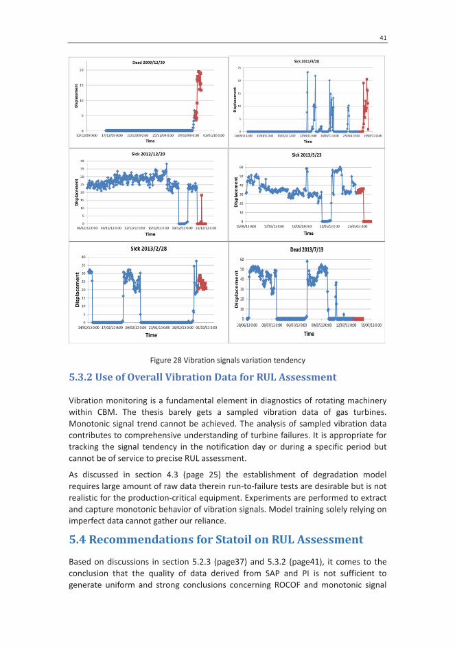
41
Figure 28 Vibration signals variation tendency
5.3.2 Use of Overall Vibration Data for RUL Assessment
Vibration monitoring is a fundamental element in diagnostics of rotating machinery within CBM. The thesis barely gets a sampled vibration data of gas turbines. Monotonic signal trend cannot be achieved. The analysis of sampled vibration data contributes to comprehensive understanding of turbine failures. It is appropriate for tracking the signal tendency in the notification day or during a specific period but cannot be of service to precise RUL assessment.
As discussed in section 4.3 (page 25) the establishment of degradation model requires large amount of raw data therein run-to-failure tests are desirable but is not realistic for the production-critical equipment. Experiments are performed to extract and capture monotonic behavior of vibration signals. Model training solely relying on imperfect data cannot gather our reliance.
5.4 Recommendations for Statoil on RUL Assessment
Based on discussions in section 5.2.3 (page37) and 5.3.2 (page41), it comes to the conclusion that the quality of data derived from SAP and PI is not sufficient to generate uniform and strong conclusions concerning ROCOF and monotonic signal

42
tendency. Failures of AC generators and gas turbines are randomly changing and unpredictable with feasible techniques. In addition, no strong relationships between notification date and failure impact are revealed.
To some extent, improving the quality of notification records is not more challenging than analyzing the data. A number of factors may have negative effects on the quality of SAP, for instance delayed reports, editing errors and missing data caused by technical problems. Table 8 illustrates current situations, challenges and corresponding suggestions to better achieve RUL assessment for Statoil. Green ones are assumed to be easy for implementation. Orange ones perhaps have some difficulties to be realized. Red ones are the most difficult issues to be handled.
Table 8 Challenges for Statoil on RUL assessment and relative recommendations Current Situation and Challenge Recommendation Specific issues Unwell, sick and dead event occurs randomly. Cannot get its reasonable sequence.
Improve the quality of SAP reports. Improve notification quality. Reexamine the nature of failure classification; maybe utilize more classification states. Build a classification system with different criteria, for instance reliability and maintenance cost.
Two comparable generators have opposite ROCOF. Cannot get a uniform failure tendency.
Check the difference in operating conditions for the two generators, such as stress and temperature. Investigate whether their spare parts are same or different.
Health condition of the equipment is unclear after each repair.
Evaluate the system’s health condition for each completed maintenance intervention, for instance as good as new and as bad as old.
Vibration signals of gas turbine do not indicate any strong monotonic trend. Cannot use it as input for RUL estimation models.
Link PI to SAP. Collect and analyze vibration data for every time the monitoring value hits the first alarm and second alarm separately and give each of these situations a failure classification. Carry out specific run-to-failure tests to collect sufficient raw data where tracks the most monotonic trend for RUL assessment.
Cannot acquire data on lubrication oil condition and acoustic noise signals. Relevant estimation models are inapplicable.
Install bespoke monitoring equipment to collect such data. Lubrication oil condition monitoring is highly recommended (see section 4.2.2, page 24)
General issues Little condition monitoring data with limited types of monitoring parameters.
Equipment experts are necessary to set valuable monitoring parameters for concerned systems. Use effective and reliable sensors to collect required large amounts of monitor data.
Matching theoretical RUL assessment models with various types of equipment.
Test research models for concerned system. Adjust model parameters. Perform necessary experiments.

43
Chapter 6 Case Study - Maintenance
Optimization
This chapter performs case study on maintenance optimization. The objective of this chapter is to link case studies to imagined current maintenance practice and future improved maintenance strategies. It is proposed to demonstrate potential savings through adopting more advanced methods using existing data in a better manner.
6.1 Introduction
As investigated in chapter 5, the thesis does not have sufficient data to develop degradation models for both AC generators and gas turbines. Statistical analysis on AC generators does not demonstrate any tendency on ROCOF. Deterioration models have difficulties to describe random failures without any regularity. It is unfeasible to correlate condition monitoring data of gas turbines to the time of failure. Traditional condition monitoring methods, for example, WT and FFT, cannot be demonstrated. The data analysis hence cannot give satisfactory results for further work on maintenance optimization. In this context, the case study conducted in this chapter is of principle where real condition data is not applied.
6.2 Degradation Models
The classification regime as previously shown in section 5.2.1.1 (page 30) is utilized. Figure 29 shows the assumed degradation process with ideal sequence of unsatisfied states. In this figure, ( )Y t is a performance variable to measure degradation processes. It describes the state of the system at time t . The first decision variable in the maintenance strategy based on this process is the inspection interval. The second one is the maintenance limit ( )Y s , which is decided by time to a sick event sT . Without any maintenance intervention, the system deteriorates into the dead state characterizing ( )Y d as failure limit.
Figure 29 Assumed degradation process

44
In the case study, the following assumptions are used:
(1) The presumed equipment is a piece of mechanical equipment. The time to a dead event is Weibull distributed with an ageing parameter 2.6α = .
(2) 1T is referred as the time to an unwell state. 2T is the time to a sick event.
3T denotes the time to a dead condition. The sum 1 2 3T T T+ + has same expected value and standard deviation as for 3T . The mean time to the dead event 3MTTF is assumed to be 100 days.
(3) It is assumed that the transition is chronologically from unwell to sick, and then dead without stepping back at any time.
6.3 Cost Model - Maintenance Optimization
This section constructs cost models for two situations with distinct maintenance strategies. As deduced in section 6.2: the first one does not perform regular inspections while the second one dose. Table 9 lists important elements to build the cost model and relevant assumed values.
Table 9 Cost elements with assumed values Cost Model Elements Assumed Value
Mean time to failure without maintenance WOMTTF =100 (days)
Ageing parameter, alpha α =2.6 The (unavailability) cost per system failure
UC =4000 (1000NOK) The cost of preventive maintenance
PMC =550 (1000NOK) The cost of corrective maintenance
CMC =800 (1000NOK) The cost per inspection
IC =5 (1000NOK)
The cost of renewing the system at state l RCC =500 (1000NOK)
These values are proposed dependent on the following arguments: (1) PMC is close to RCC . PMC in maintenance policy (a) is the cost of replacing
a unit or performing a complete overhaul preventively. It is similar to RCC , the renewal cost in (b). Even though replacing a ‘sick’ unit is costly than an ‘unwell’ one, RCC on different states should be expected in the same order of magnitude with PMC . This is due to the consideration that (i) preventive maintenance and renewal actions can all be planned in advance, for instance, plan for shutdown, make spare parts available and bring personnel for maintenance work; and (ii) both activities bring the item to a “as good as new” condition.
(2) CMC is higher than PMC and RCC . CMC is the corrective maintenance cost where cannot be planned and unexpected. The unit is perhaps in a state with severe damages. A repair is more demanding in this case.
(3) UC is the highest. UC is the unavailability cost related with the system failure. It is extremely costly in the O&G industry since the production is completely lost during the unexpected repair. 5U CMC C= is utilized.

45
(4) IC is the lowest since condition monitoring techniques could be used for inspection and that average cost is rather low.
Cost Model with No Inspection – Based on BRP
First consider a traditional maintenance strategy where no inspection is carried out. The block replacement policy (BRP) best fits the case taking into account the presence of minimal or imperfect repair. Let τ denotes the preventive maintenance interval. ( )Eλ τ denotes the effective failure rate.
Total cost per unit time: ( ) / ( ) ( )PM CM U EC C C Cτ τ λ τ= + + ×
The excel spreadsheet “BRPSImple.xls” given by course PK8207 is employed to get the result of τ and ( )C τ , see the result copy shown in figure 30. The preventive maintenance interval is 41 days with a total cost per unit time approximately 22 (1000NOK). The standard deviation in the time to failure = coefficient of variance×
WOMTTF =0.41314*100=41.314 and its variance is 1706.85, where the coefficient of variance is found by the same excel spreadsheet.
Figure 30 Result of cost per unit time without inspection
Cost Model with Inspection – Based on Markov State Model
The second maintenance strategy is considered to be improved and executed with inspections. With a finite number of states, Markov state model with inspections is utilized to demonstrate this policy.
Total cost per unit time: ( , ) / ( ) ( , ) ( , )I CM U E RCC l C C C l C rr lτ τ λ τ τ= + + × + ×
The excel spreadsheet “MaintOp.xlsm” given by course PK8207 is employed to get the result of ( , )E lλ τ , ( , )rr lτ and ( )C τ , see the result copy shown in figure 31. The system is supposed to start in a perfect state and jumps to a higher state ( iy to 1iy + ) with a time independent intensity iλ where 0,1,2i = . τ under this policy refers as inspection interval. Let 2 0/V λ λ= to model the assumed the increasing ROCOF. The factor V is used to describe how much faster failure progression is just before failure in contrast with the initial (perfect) state. Let l to be the maintenance limit, where the system is replaced with a new one if the state at an inspection is greater or equal than the limit state. Practically there is a probability q to assess the performance of inspection. For simplicity, q is assumed to be 0. Let ( , )E lλ τ denotes the effective failure rate and ( , )rr lτ signifies the renewal rate where their values are derived in an excel sheet.

46
In order to achieve the “correct” WOMTTF and its variance, the number of state r and factor V are varied. It is found that the variance of T1 + T2 + T3 is close to the variance in the time to failure in BRP when r is set to be 7 and V is 4. The standard variance is coefficient of variance × WOMTTF = 0.41467 100× =41.467 and the variance is 1719.51, where the coefficient of variance is derived by the same excel spreadsheet. Further the maintenance limit is considered to be 5. The previous “unwell-sick-dead” is not used since such situation generates a large variance compared to the one in BRP.
Figure 31 Result of cost per unit time with inspection
Maintenance Program
Table 10 presents the result comparison on two cost models. Maintenance strategy with inspections has the lower value and therefore is the cost-optimal alternative.
Table 10 Result comparison Maintenance Strategy Total cost per unit time Without inspection Approximately 22 (1000NOK) With inspection Approximately 10 (1000NOK)
The maintenance program is recommended to be built dependent on Markov state model with inspections. Its inspection interval is 5 days. The improved strategy with inspections contributes to nearly 50% cost savings.
6.4 Result Discussion
Seven states are considered to stick the Markov state model. These states can be determined by setting a specific monitoring value for each of them, for instance velocity and acceleration of rotating machinery. The lowest value indicates the best condition while the highest denotes the dead state. Equipment specialists are required to set these critical values. The inspection interval of 5 days is not realistic on condition that condition monitoring methods are employed. It is a challenge for the Markov state model to demonstrate this process with a finite number of states.
Since the procedures to establish the optimal maintenance program are dependent on assumed deterioration models and cost values, in practice, the program will vary on condition that distinct degradation models are applied as well as real costs are considered. It is expected that the maintenance strategy with inspections is the optimum since the inspection cost is rather low, particularly with applied condition monitoring techniques.

47
Chapter 7 Summary and Recommendations
for Further Work
Chapter 7 summarizes the thesis and discusses some recommendations for future work.
7.1 Summary and Conclusions
In overall, it is concluded that the main objectives of this thesis have been realized. A brief summary of achievements is presented below related to each objective.
Objective 1 - Review the literature regarding various use of the term residual useful life as a basis for giving an explicit definition to be used through the work.
The various use of the term RUL is investigated and summarized in chapter 2, where a comprehensive literature review on RUL assessment is performed. Challenges within RUL assessment are indicated, followed by a terminology study to interpret RUL in different aspects. In maintenance engineering, the RUL links to diagnostics and prognostics. The purpose is to use automated methods to analyze the equipment degradation and calculate the acceptable remaining life before the critical failure; therein condition monitoring techniques and appropriate monitoring data processing methods are significant. The statistical perspective to describe RUL has two cases, one for repairable items, and the other for non-repairable items. Reliability models as well as statistical theory are critical elements in explaining RUL from this view. The state-of-the-art RUL assessment methods are presented in table B. 1 (pageTable B. 1 Summary of various RUL estimation methods 54).
An explicit definition of RUL is determined by measures applied to evaluate the usefulness of concerned equipment. Chapter 3 proposes a new approach to define RUL based upon this principle. Table 1 (page 17) provides a preliminary solution for evaluation of equipment usefulness. Figure 9 (page 18) shows a conceptual diagram applicable for RUL assessment.
Objective 2 - Identify two to three classes of critical equipment types as a basis for case studies. Such classes could be rotating equipment, static equipment and safety systems.
Rotating equipment has been chosen as the first type of production-critical equipment at the Kristin field for the pilot investigation as the results of discussions in the R&D project executed by SINTEF/NTNU. Electrical equipment also attracts the interests of Statoil, but was not handled in the thesis work due to project constraint and time limitation.
Objective 3 - For each of the identified classes the literature shall be revived with respect to which deterministic, probabilistic and combined models are proposed to link technical condition indicators and other degradation measures to RUL.

48
Deterministic, probabilistic and combined models that link degradation behavior to RUL are referred as RUL assessment methodologies. Chapter 4 carries out revived literature investigation on such methods with rotating equipment concentrated. Major failure causes are first reviewed. Analyzing vibration signals, lubrication oil condition and acoustic noise signals contribute to rotating machinery failure detection and RUL prediction.
Two phases are required to assess the RUL of rotating equipment. The first stage is to establish degradation model dependent on run-to-failure data. Signal processing techniques, for instance WT and FFT, are used to obtain the most monotonic degradation behavior during the run-to-failure tests. The time to failure can be determined by the point of time when the RMS hit the threshold value where could be set by equipment specialists. The second stage is to predict future health condition of the equipment based on established behavior models. Degradation behavior models have many branches developed through various experiments, for example ε -Support Vectors Regression model continuous, hidden Markov model and Gaussians hidden Markov models.
Objective 4 - Select one or two cases where models, methods and real condition data could be applied in the aging and life extension management.
Reaching an agreement with the supervisor and R&D project team, AC generators and gas turbines are targets for the case studies. Chapter 5 performs statistical analysis on SAP data of AC generators and vibration signal trend analysis on gas turbine B. The analytical methods are limited by the data type we get which is notification event data and sampled vibration data.
For AC generators, the analysis does not reveal any statistically significant ROCOF. The notifications are not demonstrating a systematic pattern. Without statistical significance, an extraordinary finding is that AC generator A has a decreasing ROCOF while AC generator B has an increasing one, whereas in reality they are in same type with identical maintenance strategy. The analysis principles are well demonstrated even though the result is not statistically significant.
The analysis of vibration signals of gas turbine B does not achieve any monotonic tendency. Some notification days record the increasing trend. A number of them show the decreasing trend. The others do not present any proneness. No strong and monotonic trend is obtained in signal change based on the sampled vibration data. This restricts the application of RUL assessment models proposed in chapter 4.
The quality of SAP and PI data is not sufficient to achieve any crucial results for RUL assessment. The main weakness in the current data is that specific systematic pattern within notifications cannot be derived. More efforts on improving reporting quality and assuring data completeness are expected as discussed in section 5.4 (page 41).
Objective 5 - The case studies shall demonstrate how the maintenance program will affect the technical condition on the equipment, and how to balance maintenance effort with other measures such as upgrading projects, renewal and modification.

49
In agreement with the supervisor, objective 5 is performed where limits to a theoretical case study through utilizing assumed deterioration models and cost values.
As summarized in objective 4, it is concluded that the data in case study is not sufficient for implementation of objective 5. Maintenance program is efficient for equipment with clear failure pattern. In particular, maintenance program is established in view of proper degradation modelling. With such considerations, chapter 6 carries out a case study on maintenance optimization following necessary assumptions. Block replacement policy and Markov state models with inspections are employed to construct cost models to optimize maintenance. The result of the principle case study shows that maintenance strategy executing inspections is the optimum. It is expected that the industry can draw on these valuable theoretical investigations as of contributions for optimal maintenance planning.
Statoil do have several upgrading projects, renewal and modification actions where are recorded. Nevertheless these notes are not open for the thesis and were not pursued.
7.2 Limitations of Approach
The approach of the thesis is subject to literature review and supervision. The literature review is limited by accessible resources with full text through NTNU library. RUL assessment is a relatively new research field where illustrates theories and experimental models as a majority. Most study papers are developed by carrying out specific laboratory tests and subsequent model trainings. With no experiments and no possibility to train any model, RUL assessment within the thesis is obviously more theoretical. Applications of assessment techniques require suitable data whereas the project team provides only event data and sampled monitoring data. The results of data analysis are not satisfactory where advanced assessment methods cannot be employed.
Several meetings with SINTEF project team and Statoil experts provide background information and sampled maintenance data of AC generators and gas turbines. The deadline of thesis is three months prior to the project ‘Kristin Regularity’. This limits the prospect of retrieving more valuable information and data from Statoil.
7.3 Recommendations for Further Work
The thesis is performed with a limitation of restricted period of time as well as limited approaches discussed in section 7.2. It is recommended to further develop and improve the thesis work. A number of suggestions are given below.
Link to theoretical work (from academic perspective)
The new way to define RUL presented in chapter 3 is considered as a start for the industry to develop RUL assessment as a tool to optimize maintenance in ageing and life extension management. Further work in developing measurements for equipment evaluation is necessary and anticipated, for example, expand and apply Table 1 (page 17) with practical cases. The positive effects in using RUL assessment

50
for optimal repair cannot be generated without clear criterion for evaluation of equipment usefulness. More efforts are required in such domain.
The conceptual diagram of RUL illustrated in figure 9 (page18) only considers one failure mechanism, fatigue, as an example. In reality equipment degradation are generally caused by several failure mechanisms. It is a challenging task to establish a realistic degradation process curve. For a specific piece of critical equipment, performing ageing tests to solve this challenge is believed to be an important step forward. The future work is advised to develop suitable methods to process test data as well as specific RUL estimation models.
Link to case study (from industrial perspective)
As previously demonstrated in section 5.4 (page 41), more efforts on RUL assessment of rotating equipment are expected in the future.
What Statoil have done:
The application of SAP and PI system provides a solid foundation for future RUL assessment as well as optimal maintenance planning. The failure classification is regarded as a start to identify available equipment states where Markov state model could be utilized. Condition monitoring of vibration on rotating equipment facilitate the early detection of failures.
Recommendations:
The failures are classified as three types: unwell, sick and dead. In reality such classification can be further developed to consider more states, in which fits the Markov state model in a better manner (section 6.4, page 46).
Lubrication oil condition is strongly recommended to be monitored for production-critical rotating machinery since this technique delivers roughly 10 times earlier warnings for machine failures compared to vibration based monitoring techniques (section 4.2.2, page 24). Noise signals can also be collected for RUL prediction and it allows for remote and non-contact monitoring of the machine in contrast with vibration analysis that requires a direct contact with the equipment (section 4.2.3, page 24).
The application of single processing techniques on acquiring mot monotonic degradation behavior is dependent on sufficient raw data collected from run-to-failure experiments (section 4.2.1, page 21). Deterioration models can be further trained and tested based on experiments in the coming performance (section 4.3, page 25). Provided with valid deterioration models and true maintenance costs, the optimal maintenance strategy could be determined as well as feasible maintenance programs.
The case study only considers rotating equipment. Electrical equipment is also crucial for safe and efficient oil and gas production. The following work could make some contributions in this aspect.

51
Appendix A Technical Background
This appendix gives a short and brief introduction of technical terminology demonstrated in the thesis where is probably not well known to readers. The relative sources that can provide an in-depth understanding of these terms, techniques and models are also indicated at the end of each part.
A.1 Empirical Mode Decomposition (Source: Wikipedia)
The empirical mode decomposition (EMD) method is the essential part of the Hilbert-Huang transform. A complicated data set can be decomposed into a finite and small number of components through using the EMD method. The EMD method reduces given data into a collection of intrinsic mode functions (IMF) where the Hilbert spectral analysis could be applied then.
The Hilbert-Huang analysis is a method to examine the IMF’s instantaneous frequency data as functions of time which shows sharp identification of embedded structures. Its final result is an energy-frequency-time distribution, named as the Hilbert spectrum. More information about the EMD and Hilbert transform can be found: Alexander D. Poularikas. 2010. Transforms and Applications Handbook, Third Edition. CRC Press.
A.2 Paris Law Model (Source: Wikipedia)
Paris law is also designated as Paris-Erdogan law. It correlates the stress intensity factor to sub-critical crack growth within a fatigue stress regime. The basic formula is
mda C KdN
= Δ , where a is the crack length, N is the number of load cycles, C
and m are material constants, KΔ is the range of the stress intensity factor. It is extensively used to predict life for fatigue cracks. More information about Paris model can be found: Xiong, J. J. and Shenoi, R. A. 2011. Fatigue and fracture reliability engineering. Springer, 22 Jan 2011. ISBN 978-0-85729-218-6.
A.3 Grey System Theory (Source: Kayacan et al., 2010)
Grey models are developed to predict the future value of a time series. It is only dependent on a set of most recent data relying on the window size of the predictor. Two assumptions are within this theory. One is that all data values are assumed to be positive in this model. The second is that the sampling frequency of the time series is fixed. The main task of grey system theory is to extract realistic governing laws of the system with given data. A general grey model is ( , )GM n m , where n is the order of the difference equation and m is the number of variables. More information about grey system theory can be found: Liu, S. F., J. Forrest and Y. Lin. 2011. Grey systems, theory and applications. Springer. ISBN 978-3-642-16157-5.

52
A.4 Diffusion Process (Source: Wikipedia)
A diffusion process is to solve a stochastic differential equation. Its mathematical definition is given as “a Markov process with continuous sample paths for which the Kolmogorov forward equation is the Fokker-Planck equation”. Examples of diffusion processes are Brownian motion, reflected Brownian motion and Ornstein-Uhlenbeck processes. Si et al. (2012) indicate that diffusion processes are capable of describing random degradation among stochastic process-based models; therein Brownian motion with a linear drift becomes popular to model degradation recently. More information about diffusion process and its applications can be found: Fuchs, C. 2013. Inference for diffusion processes. Springer. ISBN 978-3-642-25969-2.
A.5 Nonlinear autoregressive exogenous model (Source: Wikipedia)
A nonlinear autoregressive exogenous model is a nonlinear autoregressive model with exogenous inputs in time series modeling. The model links the current value of a time series to past values of the same time series and current and past values of the exogenous series. It can be demonstrated as
1 2 3 1 2 3( , , , ..., , , , , ...)t t t t t t t t ty F y y y u u u u ε− − − − − −= + . y is the interested variable which we intend to predict and u is the variable determined externally. Here ε is the error term (or noise). The function F can be a neural network, a wavelet transform, etc. More information about this model can be found: Nelles, O. 2001. Nonlinear system identification. Springer. ISBN 978-3-662-04323-3.
A.6 Artificial Neural Network (Source: Wikipedia)
Artificial neural networks are computational models that are able of machine learning and pattern recognition. The networks are commonly demonstrated as systems of interconnected ‘neurons’ which computes values from inputs by feeding information through the network. This method is used to solve tasks that are difficult to find solutions using ordinary rule-based programming. More information can be found: B. Yegnanarayana. 2009. Artificial neural networks. PHI Learning Pvt. Ltd., 14. Jan. 2009.
A.7 Levenberg-Marquardt Algorithm (Source: Wikipedia)
The Levenberg-Marquardt algorithm is also designated as the damped least-squares method. It is used to solve problems facing non-linear least squares. This algorithm is known as a popular approach to solve generic curve-fitting problems. For instance, given a set of m empirical datum pairs of independent and dependent variables,
( , )i ix y , the sum of the squares of the deviations 2
1( ) [ ( , )]
m
i ii
S y f xβ β=
= − will be

53
minimal if the parameters β of the model curve ( , )f x β is optimized. The other application of Levenberg-Marquardt algorithm lies in solving nonlinear inverse problems. More information about this theory and its implementation can be found: Naveen, M., S. Jayaraman, V. Ramanath and S. Chaudhuri. 2010. Modified Levenberg Marquardt Algorithm for Inverse Problems. Lecture notes in computer science volume 6457, pp 623-632.
A.8 ε -Support Vector Regression (Source: Loutas et al., 2013)
The concept of ‘support vector machines’ is introduced by Vapnik(1995) for solving classification and regression problems. Given a set of n observations, generally, each of them lies in an M-dimensional space, M
ix R∈ , 1,...,i n= . For each observation vector, a required mapping is presented. It is further assumed that a set of target values iy R∈ contains the vector of mappings. The objective of regression is to find
a transformation f , which fulfills in the best way. The support vector context gives a good answer to this problem: Given a parameterization ( ) w xTf x b= + , find w that minimizes
1
min 1 1w w+C max( (x ) , 0)w 2
nT
i ii
y fn
ε=
− − . ε -SVR comes from the second term
of the function, which is an ε -intensive cost function. Details concerning the application of support vector regression can be found in the book Christmann and Steinwart, 2008. Support Vector Machines. Information Science and Statistics. Springer, ISBN:978-0-387-77241-7.
A.9 Principal Component Analysis (Source: Wikipedia)
Principal component analysis (PCA), a statistical procedure, uses orthogonal transformation to transfer a number of observations that are possibly correlated variables into a set of linearly uncorrelated variables, named principal components. Mathematically, PCA is an orthogonal linear transformation that converts the data to a new coordinate system. The first principal component has the greatest variance by some projection of the data. Correspondingly, the second coordinate has the second greatest variance, and so forth. Further knowledge about PCA could be found: Jolliffe I.T. Principal Component Analysis, Series: Springer Series in Statistics, 2nd ed., Springer, NY, 2002, XXIX, 487 p. 28 illus. ISBN 978-0-387-95442-4

54
Appe
ndix
B T
able
s
Tabl
e B.
1 S
umm
ary
of v
ario
us R
UL
estim
atio
n m
etho
ds
RUL
estim
atio
n m
etho
dolo
gy
Refe
renc
e/Ar
ticle
No.
Ge
nera
l top
ics
Spec
ific
syst
em/c
ompo
nent
Ph
ysic
s bas
ed m
etho
dolo
gy fo
r RU
L es
timat
ion
Ph
ysic
al M
odel
Ghio
cel (
2003
) (1)
U
sing
prob
abili
stic
ph
ysic
s-ba
sed
mod
el
to
pred
ict
RUL
incl
udin
g un
cert
aint
ies
in
mai
nten
ance
ac
tiviti
es.
-Airc
raft
jet e
ngin
es
Huan
g et
al.
(201
0) (2
) RU
L es
timat
ion
by
anal
yzin
g em
piric
al m
ode
deco
mpo
sitio
n.
-CN
C fe
ed d
rive
syst
em
Copp
e et
al.
(201
2) (3
) U
sing
Paris
law
mod
el t
o es
timat
e RU
L co
nsid
erin
g ad
just
men
t of
m
odel
par
amet
ers.
-Pla
te
Hao
et a
l. (2
012)
(4)
Fini
te
elem
ent
mod
el
with
cr
ack.
Pr
edic
t RU
L of
the
gear
with
cra
ck.
-Gea
rbox
Lort
on e
t al.
(201
3) (5
) RU
L es
timat
ion
usin
g on
line
info
rmat
ion.
Mod
elin
g de
terio
ratio
n us
ing
Mar
kov
proc
ess.
-Pne
umat
ic v
alve
s
Zhu
et a
l. (2
013)
(6)
RUL
estim
atio
n of
th
e pa
rtic
le
cont
amin
ated
lub
ricat
ion
oil
base
d on
phy
sical
mod
els.
-Win
d tu
rbin
e
Haza
rd R
ate
(P
ropo
rtio
nal h
azar
d ra
te)
Wan
g et
al.
(200
2) (7
) Fa
ilure
beh
avio
r mod
elin
g.
-Aut
omob
ile c
ompo
nent
s Ll
oyd
et a
l. (2
005)
(8)
Fram
ewor
k fo
r rel
iabi
lity
estim
ates
. ---
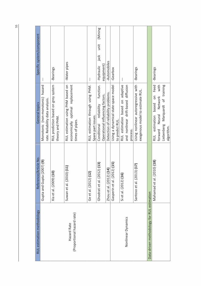
55
RUL
estim
atio
n m
etho
dolo
gy
Refe
renc
e/Ar
ticle
No.
Ge
nera
l top
ics
Spec
ific
syst
em/c
ompo
nent
Haza
rd R
ate
(P
ropo
rtio
nal h
azar
d ra
te)
Gupt
a an
d Gu
pta
(200
7) (9
) M
onot
onic
(no
n-m
onot
onic
) ha
zard
ra
te. R
elia
bilit
y da
ta a
naly
sis.
---
Xia
et a
l. (2
009)
(10)
RU
L pr
edic
tion
base
d on
gre
y sy
stem
th
eory
and
PHM
.
-Bea
rings
Suw
an e
t al.
(201
0) (1
1)
RUL
estim
atio
n us
ing
PHM
bas
ed o
n ec
onom
ical
ly
optim
al
repl
acem
ent
times
of p
ipes
.
-Wat
er p
ipes
Ge e
t al.
(201
2) (1
2)
RUL
estim
atio
n th
roug
h us
ing
PHM
. Sp
are
part
issu
es.
---
Ghod
rati
et a
l. (2
012)
(13)
Co
nditi
onal
re
liabi
lity
func
tion.
O
pera
tiona
l inf
luen
cing
fact
ors.
-H
ydra
ulic
ja
ck
unit
(Min
ing
equi
pmen
t)
Zhou
et a
l. (2
012)
(14)
De
tect
ion
of re
liabi
lity
prob
lem
s.
-Aut
omob
iles
N
onlin
ear D
ynam
ics
Gasp
erin
et a
l. (2
012)
(15)
U
sing
a dy
nam
ical
sta
te-s
pace
mod
el
to p
redi
ct R
UL.
-G
earb
ox
Si e
t al.
(201
2) (1
6)
RUL
estim
atio
n ba
sed
on a
dapt
ive
and
nonl
inea
r dr
ift-b
ased
diff
usio
n pr
oces
s.
---
Sant
oso
et a
l. (2
013)
(17)
U
sing
nonl
inea
r au
tore
gres
sive
with
ex
ogen
ous m
odel
to e
stim
ate
RUL.
-Bea
rings
Data
-driv
en m
etho
dolo
gy fo
r RU
L es
timat
ion
Mah
amad
et a
l. (2
010)
(18)
RUL
estim
atio
n ba
sed
on
Feed
fo
rwar
d N
eura
l N
etw
ork
with
Li
eben
berg
M
arqu
ardt
of
tr
aini
ng
algo
rithm
.
-Bea
rings

56
RUL
estim
atio
n m
etho
dolo
gy
Refe
renc
e Ge
nera
l top
ics
Spec
ific
syst
em/c
ompo
nent
Neu
ral N
etw
ork
Yan
et a
l. (2
011)
(19)
RU
L pr
edic
tion
base
d on
a n
eura
l ne
twor
k an
d a
new
pe
rform
ance
de
grad
atio
n in
dex.
-Rot
or u
nbal
ance
d te
st b
ed
Ahm
adza
deh
and
Lund
berg
(20
13b)
(2
0)
Usin
g ar
tific
ial
neur
al
netw
ork
to
estim
ate
RUL.
-G
rindi
ng m
ill li
ners
Cand
elie
ri et
al.
(201
3) (2
1)
Usin
g ar
tific
ial n
eura
l net
wor
ks fo
r RU
L es
timat
ion
com
bine
d w
ith fi
nite
el
emen
ts si
mul
atio
n.
-Airc
raft
stru
ctur
es
Su
ppor
t Vec
tor M
achi
ne
Scan
lon
and
Berg
in (2
007)
(22)
RU
L es
timat
ion
base
d on
sup
port
ve
ctor
m
achi
ne
and
anal
ysis
of
acou
stic
noi
se si
gnal
.
-Bea
rings
Tran
et a
l. (2
012)
(23)
RU
L es
timat
ion
base
d on
sup
port
ve
ctor
m
achi
ne
asso
ciat
ed
with
tim
e-se
ries t
echn
ique
s.
-Low
met
hane
com
pres
sor
Benk
edjo
uh e
t al.
(201
3) (2
4)
RUL
estim
atio
n ba
sed
on i
som
etric
fe
atur
e m
appi
ng
redu
ctio
n te
chni
que
and
supp
ort
vect
or
regr
essio
n.
-Bea
rings
Zhan
g et
al.
(201
3) (2
5)
Revi
ew
of
appl
icat
ions
of
us
ing
supp
ort
vect
or m
achi
ne t
o pr
edic
t RU
L.
---
Baye
sian
Net
wor
k
Ferr
eiro
et a
l. (2
011)
(26)
RU
L es
timat
ion
base
d on
a B
ayes
ian
netw
ork.
Disc
ussio
n of
mai
nten
ance
st
rate
gies
.
-Airc
raft
s
Tobo
n-M
ejia
et a
l. (2
012)
(27)
RU
L es
timat
ion
base
d on
dyn
amic
al
Baye
sian
netw
orks
. -C
NC
tool
Mos
alla
m e
t al.
(201
3) (2
8)
Pred
ictio
n of
RU
L us
ing
a Ba
yesia
n ap
proa
ch.
-B
atte
ries

57
RUL
estim
atio
n m
etho
dolo
gy
Refe
renc
e Ge
nera
l top
ics
Spec
ific
syst
em/c
ompo
nent
Baye
sian
Net
wor
k
Peng
et a
l. (2
013)
(29)
RUL
estim
atio
n ba
sed
on
Lam
b w
ave-
base
d da
mag
e de
tect
ion
tech
niqu
e an
d a
Baye
sian
upda
ting
met
hod.
-Fus
elag
e la
p jo
ints
Hidd
en (M
arko
v, Se
mi M
arko
v)
Zhan
g an
d Ka
ng (2
010)
(30)
U
sing
hidd
en
Mar
kov
and
an
infe
renc
e al
gorit
hm to
est
imat
e RU
L.-B
earin
gs
Peng
and
Don
g (2
011)
(31)
Hi
dden
M
arko
v. Ag
eing
fa
ctor
s.
Haza
rd R
ate.
-H
ydra
ulic
pum
ps
Dong
and
Pen
g (2
011)
(32)
Se
gmen
tal
hidd
en
sem
i-Mar
kov.
Agei
ng fa
ctor
s.
-Hyd
raul
ic p
umps
Tobo
n-M
ejia
et a
l. (2
011)
(33)
Es
timat
ion
of R
UL
base
d on
mix
ture
of
Gau
ssia
ns H
idde
n M
arko
v M
odel
s.-B
earin
gs
Koba
yash
i et a
l. (2
012)
(34)
U
sing
hidd
en
Mar
kov
mod
els
to
fore
cast
the
dete
riora
tion
proc
ess.
-In
frast
ruct
ures
Yu (2
012)
(35)
U
sing
hidd
en
Mar
kov
mod
el
and
cont
ribut
ion
anal
ysis
met
hod
to
asse
ss
the
mac
hine
he
alth
de
grad
atio
n.
-Bea
rings
Hybr
id a
ppro
ach
for R
UL
estim
atio
n
St
atist
ical
Mod
el
Bosk
oski
et a
l. (2
012)
(36)
RU
L es
timat
ion
base
d on
Gau
ssia
n pr
oces
s mod
els.
-B
earin
gs
Goto
and
Ken
ta (2
012)
(37)
RUL
eval
uatio
n ba
sed
on
a de
terio
ratio
n m
odel
. M
odel
pa
ram
eter
s ar
e es
timat
ed b
y us
ing
the
expo
nent
ially
wei
ghed
rec
ursiv
e le
ast s
quar
es m
etho
d.
-Rot
atin
g eq
uipm
ent
in a
the
rmal
po
wer
pla
nt.
Sank
arar
aman
et a
l. (2
013)
(38)
RU
L es
timat
ion
usin
g in
vers
e fir
st-o
rder
relia
bilit
y m
etho
d.
-Aer
ospa
ce c
ompo
nent
s

58
RUL
estim
atio
n m
etho
dolo
gy
Refe
renc
e Ge
nera
l top
ics
Spec
ific
syst
em/c
ompo
nent
Stat
istic
al M
odel
Lort
on e
t al.
(201
3) (3
9)
Prob
abili
stic
pr
ogno
sis
used
to
pr
edic
t RU
L.
---
Xi e
t al.
(201
3) (4
0)
RUL
estim
atio
n ba
sed
on
heal
th
inde
x sy
stem
s an
d Co
pula
-bas
ed
mod
els.
-Ele
ctric
coo
ling
fans
Co
mpu
tatio
nal i
ntel
ligen
ce
tech
niqu
es (F
uzzy
Log
ic, G
enet
ic
Algo
rithm
s etc
.)
Zio
and
Mai
o (2
010)
(41)
RU
L es
timat
ion
usin
g a
fuzz
y sim
ilarit
y-ba
sed
appr
oach
. -A
ccel
erat
or d
riven
syst
em
Ishi
bash
i and
Juni
or (2
013)
(42)
RU
L es
timat
ion
base
d on
ge
netic
fu
zzy
rule
-bas
ed s
yste
m s
uppo
rted
by
a d
ecisi
on tr
ee.
-Aer
onau
tical
eng
ines
Zein
-Sab
atto
et a
l. (2
013)
(43)
RU
L es
timat
ion
base
d on
non
linea
r ex
pone
ntia
l pr
edic
tion
met
hod
and
fuzz
y lo
gic
infe
renc
e sy
stem
s.
-Tur
bofa
n en
gine
com
pone
nts
W
avel
et T
rans
form
Ana
lysis
with
St
atist
ical
Mod
el
Wan
g an
d M
iao
(201
0) (4
4)
Usin
g w
avel
et
liftin
g sc
hem
e an
d hi
dden
Mar
kov
mod
el t
o de
scrib
e RU
L of
gea
rbox
.
-Gea
rbox
Tobo
n-M
ejia
et a
l. (2
011)
(45)
RU
L es
timat
ion
base
d on
Wav
elet
Pa
cket
De
com
posit
ion
and
the
mix
ture
of G
auss
ians
Hid
den
Mak
rov
Mod
els.
-Bea
rings
Lout
as e
t al.
(201
3) (4
6)
RUL
estim
atio
n ba
sed
on
-sup
port
ve
ctor
regr
essio
n.
-Bea
rings
Dyna
mic
wav
elet
with
neu
ral
netw
ork
Gebr
aeel
and
Lay
ley
(200
8) (4
7)
RUL
estim
atio
n ba
sed
on d
ynam
ic
wav
elet
ne
ural
ne
twor
k an
d Ba
yesia
n ap
proa
ches
.
---
Four
ier t
rans
form
with
neu
ral
netw
ork
Hong
mou
and
Zei
n-Sa
batt
o (2
001)
(4
8)
RUL
estim
atio
n ba
sed
on s
pect
ral
anal
ysis
usin
g Fo
urie
r Tr
ansf
orm
and
m
onito
red
vibr
atio
n sig
nals.
-Bea
rings

59
Ta
ble
B. 2
Com
paris
on v
ario
us a
ppro
ache
s for
RU
L as
sess
men
t (su
mm
arize
d fr
om A
hmad
zade
h &
Lun
dber
g, 2
013a
)
Ph
ysic
s bas
ed m
etho
dolo
gy
Expe
rimen
tal a
ppro
ache
s Da
ta-d
riven
app
roac
hes
Adva
ntag
es
Very
acc
urat
e if
the
syst
em
has
cons
isten
t ph
ysic
s of
m
odel
s.
Few
er
data
is
requ
ired
in
cont
rast
w
ith
data
-driv
en
tech
niqu
es.
Relia
ble
resu
lts
thro
ugh
acce
lera
ting
test
s ca
n be
ob
tain
ed.
Avai
labl
e to
pe
rform
th
e tr
end
anal
ysis
depe
nden
t on
th
e ex
perim
enta
l dat
a.
Do
not
requ
ire
to
assu
me
and
estim
ate
phys
ics p
aram
eter
s.
Able
to
ha
ve
a be
tter
un
ders
tand
ing
of t
he d
egra
datio
n pr
oces
s.
The
calc
ulat
ion
and
pred
ictio
n of
fu
ture
stat
es a
re e
asy.
A
wel
l-con
stru
cted
th
eore
tical
ba
sis.
The
utili
zatio
n of
mor
e co
mpl
ete
info
rmat
ion
incr
ease
es
timat
ion
accu
racy
. Di
sadv
anta
ges
Onl
y gi
ve o
vera
ll es
timat
es fo
r id
entic
al u
nits
, not
suita
ble
for
units
ope
ratin
g in
divi
dual
ly.
Expe
nsiv
e fo
r com
puta
tion.
Th
e ex
amin
atio
n of
sim
plify
ing
assu
mpt
ions
is
requ
ired.
N
orm
ally
too
sto
chas
tic a
nd
com
plic
ated
to
m
odel
th
e de
fect
.
Theo
retic
al
mod
els
are
need
ed t
o be
ver
ified
all
the
time.
M
odel
pa
ram
eter
s va
ried
easil
y in
co
nstr
aine
d co
nditi
ons.
Ex
perim
ents
are
cos
tly.
The
signi
fican
ce
of
the
expe
rimen
ts
mig
ht
be
redu
ced
by sc
alin
g pr
oble
ms.
Requ
ire la
rge
amou
nt o
f dat
a to
be
accu
rate
. Ca
n le
ad t
o in
accu
rate
tim
es o
f ch
ange
fore
cast
s.
Have
a sh
ort p
redi
ctio
n ho
rizon
. Pe
rform
po
orly
w
ith
high
di
men
siona
l dat
a.
Hard
to fi
t dom
ain.

60
Bibliography
Al-Badour, F., M. Sunar and L. Cheded. 2011. Vibration analysis of rotating machinery using time-frequency analysis and wavelet techniques. Mechanical Systems and Signal Processing. Volume 25, Issue 6, August 2011, Pages 2083-2101.
Adriaan, V. H., L. Pintelon and P. Muchiri. 2010. Maintenance optimization models and criteria. International Journal of Sys. Ass. Eng. & Man. September 2010. Volume 1, Issue 3, pp189-200.
Ahmadzadeh, F. and J. Lundberg. 2013a. Remaining useful estimation: Review. International Journal of System Assurance Engineering and Management. DOI 10.1007/s13198-013-0195-0
Ahmadzadeh F. and J. Lundberg. 2013b. Remaining useful life prediction of grinding mill liners using an artificial neural network. Miner Engineering. doi:10.1016/j.mineng.2013.05.026
Antonio, C., R. Sormani, G. Arosio, I. Giordani and F. Archetti. Assessing structural health of helicopter fuselage panels through artificial neural networks hierarchies. Source: International Journal of Reliability and Safety, v 7, n 3, p 216-234, 2013.
Atoui, I., H. Meradi, R. Boulkroune, R. Saidi and A. Grid. 2013. Fault detection and diagnosis in rotating machinery by vibration monitoring using FFT and Wavelet techniques. Systems, Signal Processing and their Applications (WoSSPA), 2013 8th international workshop on.
Banjevic, D. 2009. Remaining useful life in theory and practice. Metrika. Volume 69, Issue 2-3, pp 337-349. DOI 10.1007/s00184-008-0220-5
Benkedjouh, T., K. Medjaher, N. Zerhouni and S. Rechak. Remaining useful life estimation based on nonlinear feature reduction and support vector regression. Source: Engineering Applications of Artificial Intelligence, v 26, n 7, p 1751-60, Aug. 2013. Database: Inspec.
Boskoski, P., M. Gasperin and D. Petelin. 2012. Bearing fault prognostics based on signal complexity and Gaussian process models. 2012 IEEE Conference on PHM, p 8.
Chakravorti, S., D. Dey and B. Chatterjee. 2013. Remaining life analysis. Recent Trends in the Condition Monitoring of Transformers. Power Systems 2013, pp261-275.
Chen, X. Z., J. S. Yu, D. Y. Tang and Y. X. Wang. 2011. Remaining useful life prognostic estimation for aircraft subsystems or components: a review. The Tenth International Conference on Electronic Measurement & Instruments. ICEMI’2011.
Coppe, A.,M. J. Pais, R. T. Haftka and N. H. Kim.2012. Using a simple crack growth model in predicting remaining useful life. Journal of Aircraft, v49, n6, p1965-73, Nov.-Dec.2012.
Da Costa, C., M. H. Mathias, P. Ramos and P. S. Girao. 2010. A new approach for real time fault diagnosis in induction motors based on vibration measurement. Source: 2010 IEEE International Instru. and Meas. Tech. Conference, I2MTC 2010 - Proceedings, p 1164-1168.
Dong, M. and Y. Peng. 2011. Equipment PHM using non-stationary segmental hidden semi-Markov model. Robotics and Computer-Integrated Manufacturing. Volume 27, Issue 3, June 2011, Pages 581-590.
Ersdal, G. & E. Hörnlund, 2008. Assessment of offshore structures for life extension. Proceedings of the ASME 27th International Conference on Offshore Mechanics and Arctic Engineering

61
Ersdal, G. & P. O. Selnes, 2010. Life extension of ageing petroleum facilities offshore. SPE International 127134
Farrar, C. R. and N. A. J. 2006. Damage prognosis: The future of structural health monitoring. Philosophical Transactions of the Royal Society, 2006, 365, 623-632.
Ferreiro, S., A. Arnaiz, B. Sierra and I. Irigoien. 2011. A Bayesian network model integrated in a prognostics and health management system for aircraft line maintenance. Source: Proceedings of the Insti. of Mech. Eng., Part G: Journal of Aero. Eng. , v 225, n 8, p 886-901, August 2011. Database: Compendex
Finkelstein, M. 2008. Failure rate and mean remaining lifetime. Failure Rate Modelling for Reliability and Risk, Springer Series in Reliability Engineering 2008, pp 9-44.
Forsthoffer, W. E. B. 2005. Forsthoffer’s rotating equipment handbooks. ISBN: 978-1-85617-472-5. Copyright@2005 Elsevier Ltd. All rights reserved. http://www.sciencedirect.com/science/book/9781856174725
Gasperin, M., D. Juricic and P. Boskoski. 2012. Prediction of the remaining useful life: an integrated framework for model estimation and failure prognostics .Source: 2012 IEEE Conference on Prognostics and Health Management, p 8 pp., 2012. Database: Inspec.
Ge, E. S., Q. M. Li and H. Li. 2012. Condition-based maintenance for multi-component systems using proportional hazards model. 31st Chinese Control Conference (CCC 2012). Proceedings, p 5418-22, 2012.
Gebraeel, N., A. Elwany and J. Pan. 2009. Residual life predictions in the absence of prior degradation knowledge. Reliability, IEEE Transactions on (Volume 58, Issue1). March, 2009.
Gebraeel, N. Z. and M. A. Lawley. 2008. A neural network degradation model for computing and updating residual life distributions. IEEE T Autom Sci Eng 5(1):154–163
Ghodrati, B., F. Ahmadzadeh, and U. Kumar. 2012. Remaining useful life estimation of mining equipment: a case study. ISMPES Proceeding, New Delhi. 2012.
Ghiocel, D. M. 2003. Probabilistic approach to component condition assessment, remaining life prediction and maintenance engineering. Source: SAE Technical Papers, 2003, 2003 SAE World Congress
Goto, S., Y. Adachi, T. Furue, Y. Uchida, M. Sueyoshi, H. Hatazaki and M. Nakamura. 2008. On-line deterioration prediction and residual life evaluation of rotating equipment based on vibration measurement. SICE Annual Conference, August 20-22, 2008.
Goto, S. and T. Kenta. 2012. On-line residual life prediction including outlier elimination for condition based maintenance. International Journal of Innovative Computing, Information and Control Volume 8, Number 3(B), March, 2012.
Gupta, R. C. and R. D. Gupta. 2007. Proportional reversed hazard rate model and its applications. Jour. of Stati. Pla. & Inf. Volume137, Issue11, Pages 3525-3536. November, 2007
Huang, B. Q., M. H. Xu, H. L. Gao, M. Zhao, X. X. Wu and J. M. Yan. 2010. CNC screw life prediction based on DFNN performance model. Source: 2010 8th World Congress on Intelligent Control and Automation (WCICA 2010), p 4554-9, 2010Database: Inspec
Hudson, B. G. 2010. Extending the life of an ageing offshore facility. Abu Dhabi International Petroleum Exhibition & Conference, Abu Dhabi, UAE, 1–4 November 2010. SPE 138654.
Heng, A., S. Zhang, C. C. Andy and J. Mathew. 2009. Rotating machinery prognostics: state of the art, challenges and opportunities. Mech. Sys. and Sign. Proce. Volume 23, Issue 3, April 2009, Pages 724-739.

62
Ishibashi, R. and C. L. N. Júnior. 2013. GFRBS-PHM: A genetic fuzzy rule-based system for PHM with improved interpretability. 2013 IEEE Inter. Conf. on Progn. and Heal. Man.
ISO 13372:2012. Condition monitoring and diagnostics of machines-Vocabulary. Standard published 10/01/2012 by International Organization for Standardization.
ISO 13381-1:2004. Condition monitoring and diagnostics of machines-Prognostics-Part 1: General guidelines. International Organization for Standardization.
Jan, T. K. and B. H. Lindqvist. 1998. TTT-based tests for trend in repairable systems data. Reli. Eng. & Sys. Saf. Volume 60, Issue 1, April 1998, Pages 13-28.
Jardine, A. K. S., L. Daming and D. Banjevik. 2006. A review on machinery diagnostics and prognostics implementing condition-based maintenance. Mech. Sys. and Sig. Pro. 20 (2006) 1483-1510.
Jin G., D. E. Matthews and Z. B. Zhou. 2013. A Bayesian framework for on-line degradation assessment and residua life prediction of secondary batteries in spacecraft. Reli. Eng. & Sys. Saf. Volume 113, May 2013, Pages 7-20.
Kayacan, E., B. Ulutas and O. Kaynak. 2010. Grey system theory-based models in time series prediction. Expert Systems with Applications. Volume 37, Issue 2, March 2010, Pages 1784-1789.
Kobayashi, K., K. Kaito and N. Lethanh. 2012. A statistical deterioration forecasting method using hidden Markov model for infrastructure management. Transportation Research Part B: Methodological, v 46, n 4, p 544-561, May 2012. Compendex
Lecture note: TPK 5170 RAMS assessment and optimization, autumn 2013. Norwegian University of Science and Technology, Trondheim.
Lecture note: PK8207 Maintenance optimization, spring 2014. Norwegian University of Science and Technology, Trondheim. http://frigg.ivt.ntnu.no/ross/elearning/PK8207/
Lloyd, G. M., T. hasselman and T. Paez. 2005. A proportional hazards neural network for performing reliability estimates and risk prognostics for mobile systems subject to stochastic covariates. Jour. of Eng. and Tech. Man. 97-106.
Lorton, A., M. Fouladirad and A. Grall. 2013. Computation of remaining useful life on a physic-based model and impact of a prognosis on the maintenance process.Proceedings of the Institution of Mech. Eng., Part O: Jour. of Ri. and Rel., v 227, n 4, p 439-449, August 2013
Loutas, T.H., D. Roulias and G. Geogoulas. 2013. Remaining Useful Life Estimation in Rolling Bearings Utilizing Data-Driven Probabilistic E-Support Vectors Regression. IEEE Transactions on Reliability, v 62, n 4, p 821-32, Dec. 2013. Inspec
Ma, Z. 2009. A new life system approach to the prognostic and health management (PHM) with survival analysis, dynamic hybrid fault models, evolutionary game theory, and three-layer survivability analysis. IEEE aerospace conference 2009 (2009)
Mahamad, A. K., S. Saon and T, Hiyama. 2010. Predicting remaining useful life of rotating machinery based artificial neural network. Source: Computers and Mathematics with Applications, v 60, n 4, p 1078-1087, August 2010. Compendex.
Mason A., O. Korostynska, S. Wylie and A. I. AI-Shamma’a. 2014. Non-destructive evaluation of an activated carbon using microwaves to determine residual life. Carbon. Volume 67, February 2014, Pages 1-9.
Maio, F. D., K. L. Tsui and E. Zio. 2013. Combining relevance vector machines and exponential regression for bearing residual life estimation. Mech. Sys. and Sig. Pro. Volume 31, August

63
2012, Pages 405-427.
Mazhar, M. I., S. Kara, and H. Kaebernick. 2007. Remaining life estimation of used components in consumer products: Life cycle data analysis by Weibull and artificial neural networks. Journal of Oper. Man. Volume 25, Issue 6, November 2007, Pages 1184-1193.
McNaught K. R., and A. T. Zagorecki. 2011. Modelling techniques to support the adoption of predictive maintenance. Comp. Eng. Ser. Sys. Decision Engineering 2011, pp 277-296.
Mosallam, A., K. Medjaher and N. Zerhouni. 2013. Bayesian approach for remaining useful life prediction. Source: Che. Eng. Tran, v 33, p 139-144, 2013. Compendex
Nabavian, M. & A. Morshed, 2010. Extending life of fixed offshore installations by integrity management: a structural overview. SPE International 138386.
Nystad, B. H. 2008. Technical condition indexes and remaining useful life of aggregated systems. Doctoral dissertation. Norwegian University of Science and Technology, Trondheim, Norway. ISBN: 978-82-471-1256-4
OREDA 2009. Offshore Reliability Data Handbook 5th Edition, Volume 1 – Topside Equipment. Prepared by SINTEF Technology and Society and sold by DNV. 2009.
Peng, T. S., J. J. He, Y. M. Liu, A. Saxena, J. Celaya and K. Goebel. 2013. Fatigue damage diagnosis and prognosis using bayesian updating. Collection of Technical Papers - 54th AIAA/ASME/ASCE/AHS/ASC Structures, Structural Dynamics and Materials Conference 2013.
Peng Y., M. Dong and M. J. Zuo. 2010. Current status of machine prognostics in condition-based maintenance: a review. The International Journal of Advanced Manufacturing Technology. September 2010, Volume 50, Issue 1-4, pp 297-313.
Peng, Y. and M. Dong. 2011. A prognosis method using ageing-dependent hidden semi-Markov model for equipment health prediction. Mechanical Systems and Signal Processing. Volume 25, Issue 1, January 2011, Pages 237-252.
Poley, J., 2012. The metamorphosis of oil analysis. Mach. Fail. Prev. Tech. (MFPT) Conference, C Section 1, Conference Proceedings, Dayton, Ohio, April 24 – 26, 2012.
Rausand, M. and A. Høyland. 2004. System reliability theory: models, statistical methods, and applications, 2nd Edition. ISBN: 978-0-471-47133-2. January 2004.
Gao, R. X. and R. Q. Yan. 2011. Wavelets, theory and applications for manufacturing. Springer. ISBN 978-1-4419-1545-0.
Sankararaman, S. and K. Goebel. 2013. Uncertainty quantification in remaining useful life of aerospace components using state space models and inverse form. ASME Proceeding, Boston, 2013.
Santoso, G.B., T. Prahasto and A. Widodo. 2013. Prognosis of bearing damage performance to industrial system using nonlinear autoregressive with exogenous (NARX). Source: 2013 International Conference on QiR (Quality in Research), p 60-3, 2013.
Scanlon, P., A. Lucent, D. F. Kavanagh and F. M. Boland. 2013. Residual life prediction of rotating machines using acoustic noise signals. Instr. and mea, IEEE tran. on. Volume 62, Issue 1.
Scanlon, P. and S. Bergin. 2007. Using support vector machines and acoustic noise signal for degradation analysis of rotating machinery. Source: Artificial Intelligence Review, v 28, n 1, p 1-15, June 2007. Database: Inspec.
Shumaker, B. D. 2011. Prognostic Methods for Predicting Remaining Useful Life of Nuclear Plant Equipment and Components. Department of Energy, USA, 2011/SBIR.

64
Si, X. S., W. B. Wang, Hu C. H. Hu, and D. H. Zhou. 2010. Remaining useful life estimation – A review on the statistical data driven approaches. European Journal of Operational Research. Volume 213, Issue1, 16 August 2011, Pages 1-14.
Si, X. S., W. B. Wang, C. H. Hu and D. H. Zhou. 2011. Remaining useful life estimation-A review on statistical data driven approaches. European Journal of Operational Research. Volume 213, Issue 1, 16 August 2011, Pages 1-14.
Si, X. S., W. B. Wang, C. H. Hu, D. H. Zhou and M. G. Pecht. 2012. Remaining Useful Life Estimation Based on a Nonlinear Diffusion Degradation Process. Source: IEEE Transactions on Reliability, v 61, n 1, p 50-67, March 2012. Database: Inspec
Si, X. S., W. B. Wang, M. Y. Chen, C. H. Hu and D. H. Zhou. 2013. A degradation path-dependent approach for remaining useful life estimation with an exact and closed-form solution. European Journal of Oper. Res. Volume 226, Issue 1, 1 April 2013, Pages 53-66.
Sikorska, J. Z., M. Hodkiewicz and L. Ma. 2011. Prognostic modelling option for remaining useful life estimation by industry. Mechanical Systems and Signal Processing. Volume 25, Issue 5, July 2011, Pages 1803-1836.
Sloukia, F., M. EI Aroussi, H. Medromi and M. Wahbi. 2013. Bearings prognostic using mixture of Gaussians hidden Markov model and support vector machine. Source: 2013 ACS International Conference on Computer Systems and Applications (AICCSA), p 4 pp., 2013
Son K.L., M. Fouladirad, A. Barros, E. Levrat & B. Lung. 2013. Remaining useful life estimation based on stochastic deterioration models: a comparative study. Reliability Engineering & System Safety, Volume 112, April 2013, Pages 165-175.
Steinebach, C. and T. A. Thorstensen. 2002. Aggregated monitoring of technical condition in industrial systems. IFToMM Sixth International Conference on Rotor Dynamics, 2002.
Suwan, P., C. L. Choi, J. H. Kim and C. H. Bae. 2010. Evaluating the economic residual life of water pipes using the proportional hazards model. Water Resources Management, v 24, n 12, p 3195-3217, 2010
Tian, Z. G., Ding Y. and Ding F. F. 2011. Maintenance optimization of wind turbine systems based on intelligent prediction tools. Innovative Computing Methods and Their Applications to Engineering Problems Studies in Computational Intelligence. Volume 357, 2011, pp 53-71.
Tobon-Mejia, D.A. ; Medjaher, K.; Zerhouni, N. and Tripot, G. 2011. Estimation of the Remaining Useful Life by using Wavelet Packet Decomposition and HMMs. Source: 2011 IEEE Aerospace Conference, p 10 pp., 2011. Database: Inspec
Tobon-Mejia, D.A., K. Medjaher and N. Zerhouni. 2012. CNC machine tool's wear diagnostic and prognostic by using dynamic Bayesian networks. Source: Mechanical Systems and Signal Processing, v 28, p 167-82, April 2012. Database: Inspec
TeCoMan Wiki. The documentation site of TeCoMan. http://raga3.sintef.no/TeCoWiki/Wiki.jsp?page=Main
Thorstensen, T. A. 2007. Lifetime profit modelling of ageing systems utilizing information about technical condition. Doctor thesis. Trondheim, December 2007. Department of Marine Technology, Norwegian University of Science and Technology.
Vapnik, V. 1995. The Nature of Statistical Learning Theory. Statistics for Engineering and Information Science, Second edition. Springer—Verlag, 1995.
Vaidya, P. and M. Rausand. 2009. Life extension of machinery in the oil and gas industry. In Proceedings of European Safety and Reliability Conference ESREL, Praha, 2009.
65
Vaidya, P. and M. Rausand. 2011. Remaining useful life, technical health, and life extension. Proceedings of the Institution of Mechanical Engineers, Part O: Journal of Risk and Reliabiltiy 2011 225: 219 DOI: 10.1177/1748007810394557.
Wang, K. S., F. S. Hsu and P. P. Liu. 2002. Modeling the bathtub shape hazard rate function in terms of reliability. Reliability Engineering and Systems Safety. Volume 75, Issue 3, March 2002, Pages 397-406.
Wang, D. and Q. Miao. 2010. On-line automatic early fault detection of rotating machinery. Source: 2010 Prognostics and System Health Management Conference (PHM 2010), p 5 pp., 2010. Database: Inspec
Watson, G. S. and W. T. Wells. 1961. On the possibility of improving the mean useful life of items by eliminating those with short lives. Technometrics 3:281-298.
Wang, M. and J. Wang. 2012. CHMM for tool condition monitoring and remaining useful life prediction. The international Journal of Advanced Manufacturing Technology. March 2012, Volume 59, Issue 5-8, pp 463-471.
Xi, Z. M., R. Jing, P. F. Wang and C. Hu. 2013. A copula-based sampling method for data-driven prognostics and health management. Source: 2013 IEEE Conference on Prognostics and Health Management (PHM), p 10 pp., 2013. Database: Inspec.
Xia, L. H., H. T. Liu, M. Zhao and H. D. Wang. 2009. Study on the remaining usage life prediction of equipment and condition-based maintenance decisions. Eighth International Conference on Machine Learning and Cybernetics (ICMLC), p 2708-12, 2009.
Yan, J. H., C. Z. Guo, X. Wang and D. B. Zhao. 2011. A Data-Driven Neural Network Approach for Remaining Useful Life Prediction. Source: Key Engineering Materials, v 450, p 544-7, 2011. Database: Inspec.
Yasniy, O., Y. Lapusta, Y. Pyndus, A. Sorochak & V. Yasniy. 2013. Assessment of lifetime of railway axle. International Journal of Fatigue, Volume 50, May 2013, Pages 40-46.
Yu, J. B. 2012. Health Condition Monitoring of Machines Based on Hidden Markov Model and Contribution Analysis. Source: IEEE Transactions on Instrumentation and Measurement, v 61, n 8, p 2200-11, Aug. 2012. Database: Inspec
Zein-Sabatto, S., J. Bodruzzaman and M. Mikhail. 2013. Statistical approach to online prognostics of turbine engine components. Source: Conference Proceedings - IEEE 2013, IEEE SoutheastCon 2013: Moving America into the Future. Database: Compendex
Zhang, L. L., Z. L. Liu, D. S. Luo, J. Li, H. Z. Huang. 2013. Review of remaining useful life prediction using support vector machine for engineering assets Source:2013 International Conference on Quality, Reliability, Risk, Maintenance and Safety Engineering (QR2MSE), p 1793-9, 2013. Database: Inspec.
Zhou, C. W., R. B. Chinnam and A. Korostelev. Hazard rate models for early detection of reliability problems using information from warranty databases and upstream supply chain. International Journal of Production Economics. Volume 139, Issue 1, September 2012, Pages 180-195.
Zhu, J. D., J. Yoon, D. He, B. Qiu and E. Bechhoefer. 2013. Online condition monitoring and remaining useful life prediction of particle contaminated lubrication oil. Source: 2013 IEEE Conference on Prognostics and Health Management (PHM), p 14 pp., 2013
Zio, E. and D. M. Francesco. 2010. A data-driven fuzzy approach for predicting the remaining useful life in dynamic failure scenarios of a nuclear system. Source: Reliability Engineering and System Safety, v 95, n 1, p 49-57, January 2010. Database: Compendex

66
Curriculum Vitae
_______________________________________________________________________________
Personal Information
Name: Bin Lu Gender: Male Date of birth: 8, February 1989 Address: Herman Krags Vei 08-42 Nationality: Chinese Email (1): [email protected] Email (2): [email protected] Telephone: +47 45170655 _______________________________________________________________________________
Education 01.2012-06.2014 Master of Science – RAMS (Reliability, Availability, Maintainability
and Safety) Program Norwegian University of Science and Technology (NTNU),
Trondheim, Norway 09.2007-07.2011 Bachelor of Engineering – Machine Design Manufacturing and
Automation Harbin University of Science and Technology (HUST), Harbin, China_______________________________________________________________________________
Language Skills Chinese: Native Speaker English: Proficient User Norwegian: Basic Learner _______________________________________________________________________________
Computer Skills CARA Fault Tree Program: Fault tree analysis MINITAB: Software for statics, process improvement, Six sigma
and quality improvement Matlab: Language of technical computing Autodesk CAD: 2D and 3D design engineering software CATIA: Solution for product design and innovation. Dassault
Systems S.A. Microsoft Office: Office suite GRIF: System analysis software platform for determining the
essential indicators of dependability: Reliability-Availability-Performance-Safety