1

User Guide Form 5500 Direct Filing Entity Bulletin: Abstract of

Form 5500

January 2018

Department of Labor

Employee Benefit Security Administration

Office of Policy and Research Version 1.0

Prepared by Actuarial Research Corporation under contract

DOL-OPS-14-D-0017

2

Table of Contents

Executive Summary ........................................................................................................ 3

I. Introduction ................................................................................................................ 4

II. Overview of the DFE Asset Spreading Process ........................................................... 6

III. Data Selection and Editing ........................................................................................ 8

IV. Missing Data ........................................................................................................... 12

V. Methodology: Algebra of DFE Ownership ............................................................... 12

VI. Application of Matrix Algebra ................................................................................ 19

VII. Spreading Pension Assets ...................................................................................... 21

VIII. Impact of Imputation ........................................................................................... 21

Technical Appendix I .................................................................................................... 25

Technical Appendix II ................................................................................................... 26

3

Starting with 2008 plan year data, the U.S. Department of Labor has published the Direct

Filing Entity (DFE) Bulletin which includes information on assets and asset spreading

across DFEs. This user guide is intended to accompany the Form 5500 Direct Filing

Entity Bulletin and will explain the data edits and methodology used to produce the

statistics in the bulletin.

Executive Summary

Each year the Employee Benefits Security Administration (EBSA) of the U.S.

Department of Labor (the Department) publishes a report containing summary statistics

on U.S. private retirement plans using the Form 5500 Annual Return/Report. The Private

Pension Plan Bulletin Abstract of Form 5500 Annual Reports presents summary

information on retirement plan counts, participant counts, and financial aggregates

(including assets by category, contributions, and benefits).

For Form 5500 reporting purposes, private pension plans either hold assets directly in the

form of cash, stocks, government securities, and mutual funds, among others, or

indirectly, in the form of investments in pooled investment arrangements. In certain

cases, the sponsors of these pooled investment arrangements are either required or can

choose to file a Form 5500 for these entities. The Form 5500 instructions identify such

entities as Direct Filing Entities (DFEs).1 Depending on whether or not a DFE files a

Form 5500, the reporting requirements for the investing pension plans differ. Pension

plans that invest in DFEs that do not file the Form 5500 are required to report all assets

on the Schedule H – Financial Information – Large Plan as if those assets were held

directly. Pension plans that invest in DFEs that file a Form 5500 can receive reporting

relief by reporting all assets invested in those DFEs on the line items for the correct DFE

types.

Due to the Schedule H reporting relief described previously, EBSA has historically

reported assets as reported on Schedule H without adjustment. The result of this

methodology is that assets are reported as being held in certain concrete categories, such

as cash, stocks, and mutual funds, while assets invested in DFEs are reported as interest

in DFEs.

In order to gain information about the investments of private pension plans, EBSA needs

to know the allocation of the financial assets held by private pension plans using only

those assets found on the non-DFE line items of Schedule H. However, assets in the

pooled investment arrangement class are comprised of assets in the financial class, but

not reported as such on Schedule H. As the statistics in the DFE bulletin will show,

almost half of the asset holdings of private pension plans in the U.S. are held in the

pooled investment arrangement class and the public disclosure using Form 5500 filings

for such plans will not show detailed investments due to the reporting relief described

above (see Form 5500 instructions for more information about the filing relief).

Therefore, EBSA has created a methodology to ‘spread’ the assets found in the pooled

1 The term DFE is unique to the Form 5500 reporting regime; however, we refer to any pooled investment

arrangement that does or could choose to file the Form 5500 as a DFE for the purposes of this document.

4

investment arrangement class into underlying financial asset categories. Thus, EBSA has

produced the Form 5500 Direct Filing Entity Bulletin Abstract of Form 5500, to

summarize the universe of DFEs and the DFE asset spreading methodology. Table 11 in

the Form 5500 Direct Filing Entity Bulletin Abstract of Form 5500 is a reproduction of

Table C4 of the Private Pension Plan Bulletins Abstract of Form 5500 Annual Reports.

Table 11 is also included in the Private Pension Plan Bulletins Abstract of Form 5500

Annual Reports as Table C4(a). This table shows the assets that were in the original four

pooled investment arrangement categories ‘spread’ into their underlying financial asset

categories. This document gives the technical details of the methodology EBSA used to

spread DFE assets into their underlying financial asset categories.

I. Introduction

Each year, many private pension plans satisfy their annual reporting requirement by filing

a Form 5500 Annual Return/Report regarding their financial condition, investments, and

operations with the U.S. Department of Labor, Internal Revenue Service (IRS), and, if

applicable, the Pension Benefit Guarantee Corporation (PBGC).2 Most plans with 100 or

more participants are required to disclose the value of the assets that the plan holds in

various asset categories using the Schedule H “Financial Information.”3

There are multiple types of assets that a plan may hold that need to be reported on the

Schedule H. Outside of direct holdings in items such as cash, stocks, or bonds, private

pension plans may also invest a portion of their asset holdings in investment vehicles

such as master trust investment accounts (MTIA), common/collective trusts (CCT),

pooled separate accounts (PSA), and other pooled investment arrangements known as

103-12 investment entities (103-12 IE). These types of investment vehicles are

collections of funds from individual investors or groups of investors that are pooled

together in order to obtain wholesale prices and rates unavailable for regular investors.

For private pension plans, master trust investment accounts (MTIA) are those for which a

regulated financial institution serves as the trustee and holds the assets of one or more

plans sponsored by a single employer, or by a group of employers under common

control.4 A common/collective trust (CCT) is maintained by banks or other financial

institutions which hold assets of plans sponsored by more than one employer or a

controlled group of corporations as the term is used in Code section 1563. Pooled

2 The Department’s Employee Benefit Security Administration’s (EBSA) Office of Policy and Research

(OPR) analyzes the Form 5500 Annual Return/Report filings of private pension plans to produce two

publications, the annual Private Pension Plan Bulletin Abstract of Form 5500 Annual Reports and the

annual Private Pension Plan Historical Tables and Graphs. 3 Plans with fewer than 100 participants are required to disclose the value of assets on the Schedule I

“Financial Information – Small Plans.” The Schedule I does not provide for reporting investment in the pooled investment arrangement class. Therefore, small plans are excluded from this report. 4 A “regulated financial institution” means a bank, trust company, or similar financial institution that is

regulated, supervised, and subject to periodic examination by a state or federal agency. A securities

brokerage firm is not a “similar financial institution” as used here. See DOL Advisory Opinion 93-21A

(available at www.dol.gov/ebsa).

5

separate accounts (PSAs) are collective investment accounts maintained by an insurance

carrier which holds assets of plans sponsored by more than one employer or a controlled

group of corporations as the term is used in Code section 1563. Finally, collective

investment accounts which are not covered by one of these three definitions are generally

referred to as 103-12 investment entities (103-12 IE).

Schedule H (financial information schedule) requests information on 24 asset categories

that need to be completed both for the beginning and for the end of the plan year. The

following is the list of those asset categories with the last four corresponding to the types

of accounts referred to as pooled investments arrangements (MTIA, CCT, PSA, 103-02

IE).

Part I, 1a – Noninterest-bearing cash

Part I, 1b(1) – Employer contributions

Part I, 1b(2) – Participant contributions

Part I, 1b(3) – Other receivables

Part I, 1c(1) – Interest-bearing cash (include money market accounts & certificates of

deposit)

Part I, 1c(2) – U.S. Government securities

Part I, 1c(3)(a) – Preferred corporate debt (other than employer securities)

Part I, 1c(3)(b) – All other corporate debt (other than employer securities)

Part I, 1c(4)(a) – Preferred stock (other than employer securities)

Part I, 1c(4)(b) – Common stock (other than employer securities)

Part I, 1c(5) – Partnership/joint venture interests

Part I, 1c(6) – Real estate (other than employer real property)

Part I, 1c(7) – Loans (other than to participants)

Part I, 1c(8) – Participant loans

Part I, 1c(9) – Value of interest in common/collective trusts

Part I, 1c(10) – Value of interest in pooled separate accounts

Part I, 1c(11) – Value of interest in master trust investment accounts

Part I, 1c(12) – Value of interest in 103-12 investment entities

Part I, 1c(13) – Value of interest in registered investment companies (e.g., mutual funds)

Part I, 1c(14) – Value of funds held in insurance company. general account (unallocated

contracts)

Part I, 1c(15) – Other

Part I, 1d(1) – Employer securities

Part I, 1d(2) – Employer real property

Part I, 1e – Buildings and other property used in plan operation

Reporting Relief

Private pension plans participating in DFEs are relieved from having to report on a line-

by-line basis on Schedule H the amount of their investments if the DFE in which the

plan is investing files a Form 5500 Annual Return/Report along with all required

schedules . In that case, the participating plans need only complete line items (Part I c(9)

through c(12)) describing the value of their interests in the DFEs, All master trust

6

investment accounts (MTIA) are required to file Form 5500, while common/collective

trusts (CCT), pooled separate accounts (PSA), and 103-12 investment entities (103-02

IE) may choose to file in order to provide the investing pension plans the reporting relief

described above. 5

All DFEs that file the Form 5500 are required to file a Schedule H.

Pension plans investing in filing DFEs are afforded reporting relief through decreased

reporting on Schedules A, C, and H; however, they must file a Schedule D, outlining the

specific investments in each filing DFE. Plans investing in DFEs will enter the value of

their investment in all DFEs of a certain type (master trusts, common/collective trusts,

pooled separate accounts, or 103-12 investment entities) on the corresponding Schedule

H line item.

The percentage of large private pension plan assets held in these categories in 2015 was:

1. Value of interest in common/collective trusts – 13.4 percent

2. Value of interest in pooled separate accounts – 2.4 percent

3. Value of interest in master trust investment accounts – 27.4 percent

4. Value of interest in 103-12 investment entities – 1.0 percent

Thus for roughly 44 percent of all assets held by large pension plans, the public

information on plans’ investments on the Form 5500 is limited to the class of the pooled

investment arrangements rather than the financial class of the underlying investments

(common stock, U.S. Government Securities, registered investment companies, etc.). In

theory the asset allocation by financial class for each pension plan investing in DFEs can

be derived from Form 5500 data (using the Schedules H and D of the pension plans, and

the Schedule H of the DFEs). However, there are technical challenges which arise due to

the fact that pension plans can and do invest in multiple DFEs, and DFEs can and do

invest in other DFEs. It is also important to note that DFEs which invest in other DFEs

can also realize the same reporting relief on Schedule H as pension plans that invest in

DFEs. These facts give rise to complicated patterns of DFE investment that can be

challenging to unravel.

II. Overview of the DFE Asset Spreading Process

EBSA uses the seven step process below to “spread” the assets both private pension plans

and DFEs hold in the pooled investment account classes:

5 The Form 5500 Instructions (Page 9) define a DFE as follows:

Some plans participate in certain trusts, accounts, and other investment arrangements that file the

Form 5500 annual return/report as a DFE. A Form 5500 must be filed for a master trust

investment account (MTIA). A Form 5500 is not required but may be filed for a

common/collective trust (CCT), pooled separate account (PSA), 103-12 investment entity (103-12 IE), or group insurance arrangement (GIA). However, plans that participate in CCTs, PSAs, 103-

12 IEs, or GIAs that file as DFEs generally are eligible for certain annual reporting relief. For

reporting purposes, a CCT, PSA, 103-12 IE, or GIA is considered a DFE only when a Form 5500

and all required schedules and attachments are filed for it in accordance with the following

instructions.

7

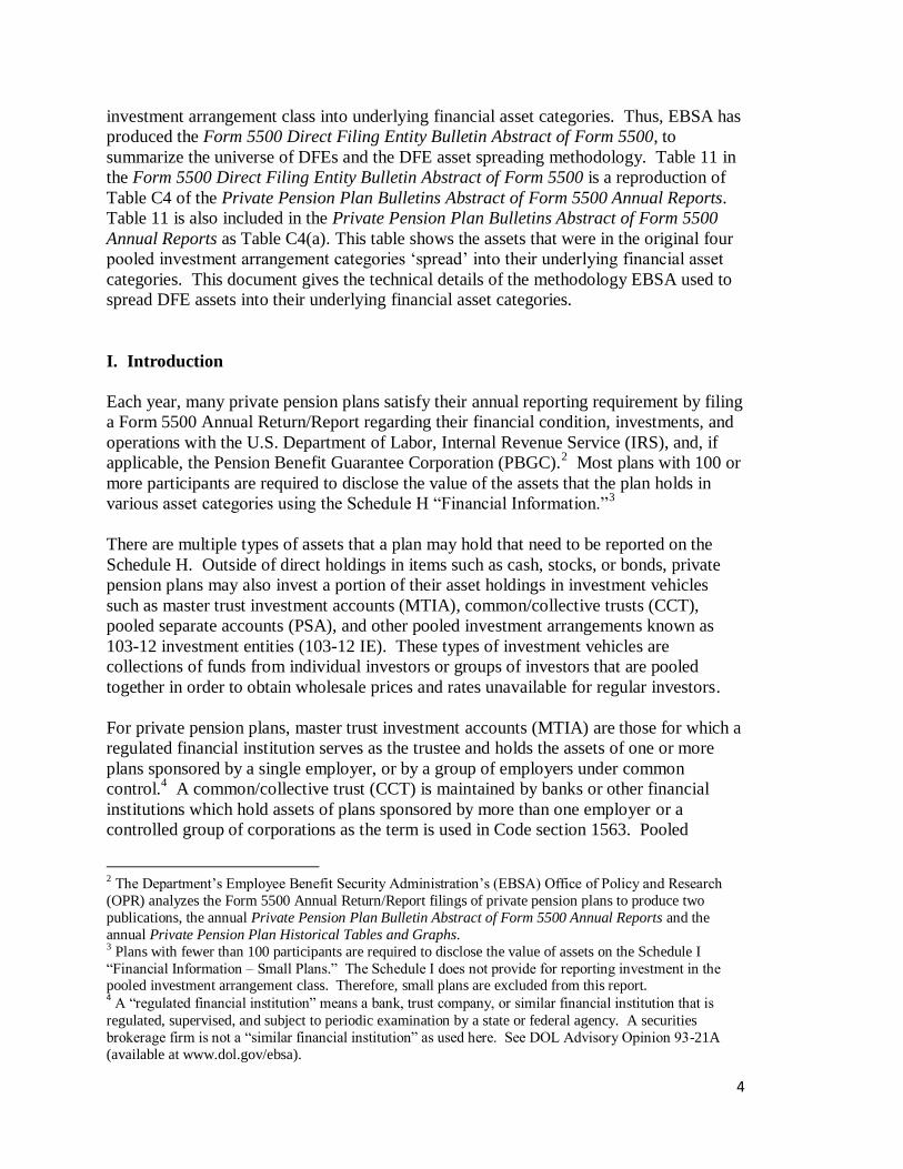
1. EBSA creates a DFE dataset by extracting and combining data from the main

Form 5500, Schedule H, and Schedule D for all DFEs which file a Form 5500.

2. EBSA edits the Schedule D data in this DFE dataset to ensure that the financial

information corresponding to interest in other DFEs reported on Schedule H is

commensurate with the information reported on the Schedule D. For instance, if DFE A

reports $1,000,000 as the value of interest in PSAs on Schedule H, it is necessary to

verify that DFE A’s Schedule D reflects $1,000,000 invested in specific PSAs. If the

Schedule H and Schedule D data differ, EBSA edits the Schedule D information to match

the Schedule H information.

3. EBSA selects only those DFEs that report investing assets in other DFEs. This

group is further reduced to include only those DFEs whose investee DFEs have Form

5500s on file with DOL. EBSA is unable to identify some DFEs (reported as holding

private pension plan or DFE assets) either because of improper reporting (for example,

the plan was mistaken in their assumption that the DFE they invest in is actually filing

their own individual Form 5500), errors in processing filings (for example, if a DFE files

a Form 5500 which was inadvertently not entered into the database), or Employer

Identification Number and Plan Number (EIN/PN) mismatches (for example if the filing

entity mistakenly reports an incorrect EIN/PN for the DFE in which they invest). The

resulting dataset can be considered a ‘closed’ DFEs dataset in that all of the included

DFE Form 5500 filings report holding assets in a DFE, for which EBSA has a linked

Form 5500 filing. In other words, EBSA identifies a Form 5500 for both the investing

DFE and all DFEs in which these invest assets. Further, all of the DFEs in this ‘closed’

dataset are unassociated with unlinked Form 5500 filings through intermediaries. For

example, if DFE A is invested in DFE B for which EBSA has a filing, but DFE B is

invested in DFE C for which EBSA does not have a filing, then neither DFEs A nor B

are included.

4. For each individual DFE in the ‘closed’ DFE dataset, EBSA spreads all of the

assets reported in Schedule H’s pooled investment arrangement asset class categories to

the financial asset class categories of Schedule H. EBSA implements its matrix algebra

approach (discussed in detail below) to determine the ownership of assets in the ‘closed’

DFE dataset. Several matrices are created to calculate the ownership of the assets of each

DFE by any other DFEs. This calculation is based on the Schedule D filings of the

individual DFEs in the ‘closed’ dataset. As a result, all of the reported holdings in pooled

investment arrangement asset classes are moved into the DFE that holds those assets.

The resulting dataset consisting of a record for each individual DFE in the ‘closed’ DFE

dataset which contains a revised Schedule H asset allocation with $0 reported as the value

in pooled investment arrangement asset classes, i.e. the ‘closed, spread’ DFE dataset.

5. The ‘closed, spread’ DFE dataset is used to impute the underlying asset

characteristics of DFEs for which EBSA is unable to locate a filing. As mentioned

above, certain DFEs are reported as holding private pension plan assets, yet the DFE

cannot be matched to a Form 5500, i.e. an ‘unlinked’ DFE Form 5500 filing. Therefore,

any assets reported as being invested in unlinked DFE Form 5500 filings are spread to the

8

various financial asset categories of Schedule H based on a hot decking imputation

method. With this method an asset allocation of a randomly selected individual DFE

from the ‘closed, spread’ DFE dataset is applied to each ‘unlinked’ DFE Form 5500

filing. The assets reported as investments in the ‘unlinked’ DFE Form 5500 filing are

‘spread’ according to the distribution of assets on the revised Schedule H of the randomly

selected DFE.

6. Once all assets reported as investments in ‘unlinked’ DFE Form 5500 filings are

spread, the matrix algebra discussed in step 4 above is repeated, this time incorporating

the ‘unlinked’ DFEs that were not previously included. The result is the ‘spread

allocation’ for the universe of DFE Form 5500 filings.

7. Finally, the DFE ‘spread allocation’ is used to distribute pension assets reported

under the pooled investment arrangement asset categories on Schedule H to the financial

asset categories. The Private Pension Plan Research File (PPP Research File) is

augmented with the corresponding data from filed Schedules D. As with the DFE Form

5500 filings, the asset information is edited to match what is reported on Schedule H.

Assets reported as investments in ‘unlinked’ DFEs are handled exactly as described in

step 5 above. Therefore using the asset allocations of the ‘spread allocation’ DFE dataset

and randomly chosen DFE Form 5500s for ‘unlinked’ DFE Form 5500 filings, all private

pension plan assets reported as interest in pooled investment arrangement classes are

moved to the financial asset classes. The assets will be moved based on the distribution

of assets for the Form 5500 DFE filings in which each private pension plan invests. This

information is presented on Table 12 of the DFE bulletin.

III. Data Selection and Editing

To complete the spreading process, two distinct sets of data are required. The first set is

partially complete before we begin the process, in the form of the PPP Research File

produced annually by EBSA. This dataset consists of information from the Form 5500,

Schedule H, and Schedule I on all large and small private pension plans.6 For use in this

project, this data must be augmented with the corresponding information from Schedule

D. Therefore, the final private pension data used for this project is an augmented version

of the PPP Research File. The Schedule H information includes end of year asset

amounts as described in the introduction, Section I above, along with the beginning of

year assets for each category, income, and expense statements. The Schedule D contains

information on all DFEs in which the filer invests. This information includes the EIN/PN

of the filer and the DFEs, the amount of assets invested in each DFE, the type of DFE,

and the name of the DFE.

The second dataset required to create the ‘spread allocation’ for both DFEs and private

pension plans is a dataset of Form 5500 filing information for all filing DFEs. DFEs

identify themselves when filing Form 5500 by checking the box (part I(A)) marked “a

6 See http://www.dol.gov/ebsa/publications/form5500dataresearch.html for more information regarding this

dataset.

9

DFE” under “This return/report is for:” on the Form 5500. The DFE additionally inputs

an “M,” “C,” “P,” or “E” next to the box. These letters correspond to master trust

investment accounts (MTIA), common/collective trusts (CCT), pooled separate accounts

(PSA), and 103-12 investment entities respectively. For all self-identified DFEs, data

from the Form 5500 is combined with Schedule H and Schedule D data included with

that filing.

Once both datasets are obtained, the information on Schedule H is compared to what has

been filed on Schedule D. In all cases, the value of assets in the pooled investment

category on the Schedule H should equal the sum of the individual investments in DFEs

of that type on Schedule D.

EBSA uses an automated editing process which logically corrects inconsistencies

between Schedules H and D. Pages 7 and 8 summarize two logical editing paths, one for

common collective trusts and pooled separate accounts, and the other for master trusts

and 103-12 investment entities. Two paths are necessary because both pension plans and

DFEs might erroneously report owning assets in common collective trusts and pooled

separate accounts that do not file a Form 5500; in these cases ‘000’ is reported for the

plan number. This path will not apply to master trust investment accounts and 103-12

investment entities, as all master trusts and 103-12 investment entities must file the Form

5500. Such amounts are reported erroneously because the Form 5500 line items for

common collective trusts and pooled separate accounts may legitimately be used only to

report holdings in trusts or accounts that file Form 5500.

For the necessary editing of Form 5500 data, there are two types of assets reported in

DFEs on Schedule D: ‘linked’ and ‘unlinked.’ ‘Linked’ assets refer to all assets held in

DFEs for which EBSA can identify a Form 5500 filing. ‘Unlinked’ assets refer to all

assets held in DFEs for which EBSA cannot identify a Form 5500 filing.

In general, Tables 1 and 2 below describe a process in which ‘unlinked’ amounts are

ignored whenever possible, and reported investments on Schedule D are scaled to match

the amounts reported on Schedule H. In this way, the individual investments reported on

Schedule D are proportional to the originally filed Schedule D but match the amounts

reported on Schedule H.

10

Table 1: Master Trusts and 103-12 Investment Entities Automatic Edits

Note: “Positive” refers to non-zero amounts, “0” refers to 0 amounts, “Any” refers to “Positive” or “0” amounts, and “>/</=H” refers to the comparison of the

cell to the value reported on Schedule H as “interest in” the DFE type.

7 Schedule H-reported holding in master trusts or 103-12 investment entities. 8 Summary of Schedule D-reported holding in master trusts or 103-12 investment entities by type of asset (“linked,” “unlinked,” and the sum of the two, defined

above.

Sch. H

Assets7

Schedule D Assets8 Comment

Linked Unlinked Total

0 0 0 0 Records are clean.

0 Any Any Any All Schedule D amounts are adjusted to 0.

Positive 0 0 0 All assets assumed to be in 1 DFE. This DFE is hot-decked.

Positive 0 Positive =H The unlinked DFEs are hot-decked.

Positive 0 Positive <H The unlinked DFEs are hot-decked and amounts are proportionately

increased to sum to the amount reported on Schedule H

Positive 0 Positive >H The unlinked DFEs are hot-decked and amounts are proportionately

decreased to sum to the amount reported on Schedule H

Positive Positive 0 =H Data are correct.

Positive Positive 0 <H Amounts are proportionately increased to sum to the amount reported

on Schedule H.

Positive Positive 0 >H Amounts are proportionately decreased to sum to the amount reported

on Schedule H.

Positive Positive Positive <H The unlinked DFEs are hot-decked and amounts are proportionately

increased to sum to the amount reported on Schedule H

Positive Positive Positive =H Unlinked DFEs are hot-decked.

Positive Pos, <H Positive >H The unlinked DFEs are hot-decked and unlinked amounts are

proportionately decreased to sum to the amount reported on Schedule H

Positive Pos, =H Positive >H Unlinked are ignored

Positive Pos, >H Positive >H The unlinked DFEs are hot-decked and all amounts are proportionately

decreased to sum to the amount reported on Schedule H

11

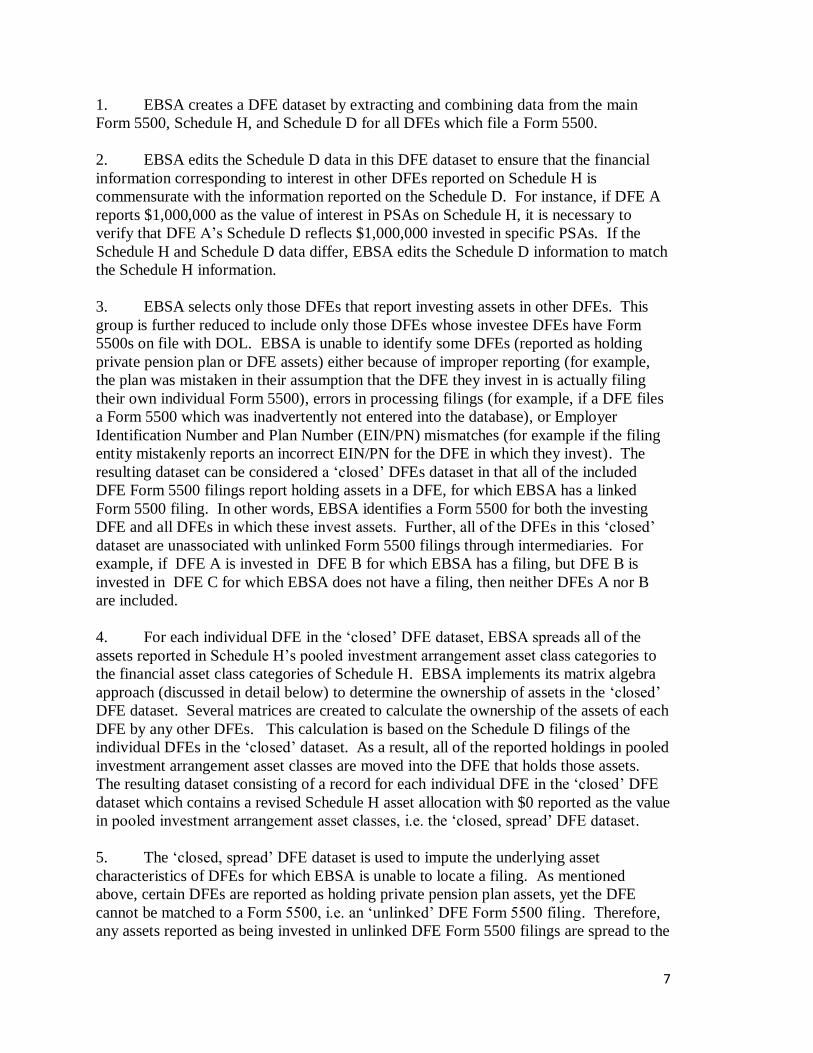
Table 2: Common Collective Trusts and Pooled Separate Accounts Automatic Edits

Note: “Positive” refers to non-zero amounts, “0” refers to 0 amounts, “Any” refers to “Positive” or “0” amounts, and “>/</=H” refers to the comparison of the

cell to the value reported on Schedule H as “interest in” the DFE type.

9 Schedule H-reported holding in master trusts or 103-12 investment entities.

10 Summary of Schedule D-reported holding in master trusts or 103-12 investment entities by type of asset (“linked,” “unlinked,” and the sum of the two, defined

above.

Sch. H

Assets9

Schedule D Assets10

Positive Plan Numbers Null or

000

Total Comment

Linked Unlinked Total

0 0 0 0 0 0 Records are clean.

0 Any Any Any Any Any All Schedule D amounts are adjusted to 0.

Positive 0 0 0 0 0 All assets assumed to be in 1 DFE. This DFE is hot-

decked.

Positive 0 0 0 Positive =H The null DFEs are hot-decked.

Positive 0 0 0 Positive <H, >H One DFE is hot-decked with amount = H.

Positive 0 Positive Any 0 =H Hot-deck unlinked DFEs

Positive 0 Positive Any 0 <H, >H Hot-deck unlinked DFEs and scale amounts to match H

Positive Any Positive =H Positive Any Hot-deck unlinked DFEs. Ignore those with null or ‘000’

Positive =H 0 =H 0 =H Records are clean.

Positive =H 0 =H Positive >H Null or ‘000’ plan numbers ignored since linked

amounts represent the full investment.

Positive =H Positive Any Any Any Unlinked, null, and ‘000 plan numbers ignored.

Positive <H, >H 0 Any 0 Any Scale linked amounts to match H.

Positive <H Any Any Any =H Hot-deck all.

Positive <H Any <H Any <H, >H

If total unlinked and null or ‘000’ is 0, row 10 applies. Otherwise, scale all amounts up to H and hot-deck all.

Positive Any Positive <H Positive =H Hot-deck all.

Positive <H Positive >H Any >H Scale back positive plan numbers to H amount and hot-

deck unlinked. Ignore null or ‘000.’

Positive >H Any Any Any Any Ignore unlinked amounts. Scale back linked

amounts.

12

In addition to the edits performed to align Schedule H and D filings, EBSA also performs limited

editing to the dataset of DFEs (in addition to the more extensive edits performed to create the

Research File).11

EBSA utilizes the OPR Editor, a Department program, to edit Form 5500 data and create the

PPP Research File. To allocate the assets reported in the four DFE asset categories to the non-

DFE asset categories, EBSA first utilizes the OPR Editor to edit the Form 5500 DFE filings. In

addition to using the OPR Editor, the DOL contractor Actuarial Research Corporation (ARC)

make edits that include, but are not limited to: deleting erroneous (non-DFE) filings from the set

of filings that self-identified as DFEs, updating employer identification numbers, and making

financial edits which were not corrected by the OPR Editor.

Once both of these datasets, one consisting of DFE filings and one consisting of private pension

plan filings, are complete, EBSA can begin the process to obtain ‘spread allocations’ for both

datasets. These datasets are processed separately, as will later become clear. The reason for this

is that private pension plans can invest in DFEs, but DFEs can never invest in private pension

plans. Therefore, inter-investment is limited to DFEs.

IV. Missing Data

In addition to inconsistencies reported on Schedules H and D, there is another source of error in

the Form 5500 data being used. For both the filing DFEs and private pension plans, some DFEs

that are reported on Schedule D cannot be found in EBSA’s data. For example, if a private

pension plan reports being invested in DFE A on its Schedule D, but EBSA can find no

corresponding Form 5500, Schedule H, or Schedule D for DFE A. In these cases, the reported

Schedule D amount invested in the missing DFE is referred to as an ‘unlinked’ amount (as

discussed above). During this process EBSA creates a subset of the DFE dataset described

above by selecting all DFEs that are unaffected by ‘unlinked’ amounts. This means that any

DFE that either directly reports an unlinked amount or reports investment in other DFEs that

report unlinked amounts are temporarily removed from the dataset. In fact, each DFE that is

associated with an unlinked amount through any number of intermediaries is temporarily

removed. As mentioned in Section II, this subset is referred to as the ‘closed’ DFE set.

V. Methodology: Algebra of DFE Ownership

The task of properly accounting for the assets that pension plans hold via DFEs is made

complicated by the fact that inter-investment among DFEs is common. To overcome this

challenge, the analysis will proceed in two phases. Phase 1 of the analysis will disentangles these

DFE inter-investments. Once this phase is complete, the one-directional allocation of assets

from DFEs to their plan investors is straightforward. When discussing phase 1, it is convenient

to speak of DFEs as “owning” whatever share of the assets they hold that are not “owned” by

11 For more information regarding the Form 5500 Research File, please refer to the current Form 5500

User Guide found at http://www.dol.gov/ebsa/publications/form5500dataresearch.html

13

other DFEs. Of course, the share of each DFE’s assets that is “owned” by the DFE itself is

actually owned by the plans whose assets it holds, but we choose to postpone discussion of

ownership by plans until phase 2 of the analysis.

The share of DFE j directly owned by DFE i depends on two factors:

The extent to which DFE i holds assets of DFE j, and

The extent to which DFE i is owned by other DFEs.

OPR begins phase 1 by recording the percentage of each DFE j directly held by every other DFE

i in a “holding matrix” A, an n x n matrix where n represents the number of DFEs for a given

year:

𝐴 =

[ 𝑎1,1 𝑎1,2 𝑎1,3 … 𝑎1,𝑛

𝑎2,1 𝑎2,2 𝑎2,3 … 𝑎2,𝑛

𝑎3,1 𝑎3,2 𝑎3,3 … 𝑎3,𝑛

⋮ ⋮ ⋮ ⋱ ⋮𝑎𝑛,1 𝑎𝑛,2 𝑎𝑛,3 … 𝑎𝑛,𝑛]

, 𝑤ℎ𝑒𝑟𝑒 𝑎𝑖,𝑗 =𝐷𝐹𝐸 𝑖 𝑖𝑛𝑣𝑒𝑠𝑡𝑚𝑒𝑛𝑡 𝑖𝑛 𝐷𝐹𝐸 𝑗

𝐷𝐹𝐸 𝑗 𝑡𝑜𝑡𝑎𝑙 𝑎𝑠𝑠𝑒𝑡𝑠.

All ai,j should be less than 1 and ai,j should always equal 0 when i = j, as a DFE should not report

direct investment in itself. Furthermore, each column of A should sum to no more than one,

because the combined holdings of all other DFEs in DFE j cannot exceed 100 percent.

For example, consider DFE A that directly holds 20 percent of DFE B, and DFE B directly holds

10 percent of DFE C. The matrix A that captures these relationships is:

𝐴 =

𝐷𝐹𝐸 𝐴 𝐵 𝐶𝐴 ⌈0.00 0.20 0.00⌉

𝐵 |0.00 0.00 0.10|

𝐶 ⌊0.00 0.00 0.00⌋

.

Next, we compute the extent to which the assets of each DFE are directly held by any other DFE

by summing the columns of A yielding n sums S1, S2,…, Sn. Note that these sums also represent

the extent to which each DFE is directly or indirectly owned by any other DFE because indirect

ownership of a DFE must pass through one or more of its direct owners.

In our example, these column totals are [0.00, 0.20, 0.10]. We compute the share of each DFE

not owned by others by subtracting each of these shares from 1, yielding [1.00, 0.80, 0.90]. a2,3

reports that DFE B holds 10 percent of DFE C. The share of DFE C owned by DFE B is the

product a2,3 x 0.80. Thus DFE B’s 10 percent holding of DFE C reflects 8 percent ownership.

We can construct a matrix M1, referred to as the first-order ownership matrix, reflecting the

extent to which each DFE directly owns each other DFE can be derived by left multiplication of

the holding matrix, A, by a diagonal matrix E with entries S1, S2, …, Sn, where 𝑆𝑘 = 1 − ∑ 𝑎𝑖,𝑘𝑛𝑖=1 ;

that is:

14

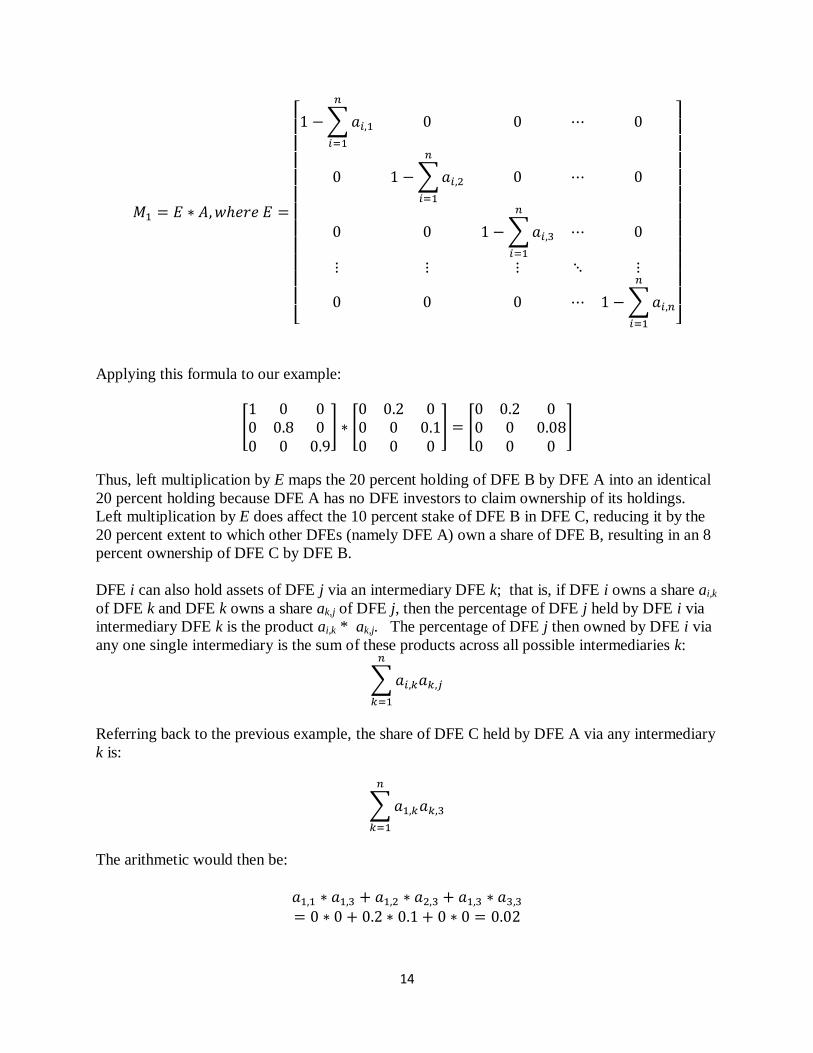
𝑀1 = 𝐸 ∗ 𝐴,𝑤ℎ𝑒𝑟𝑒 𝐸 =

[ 1 − ∑𝑎𝑖,1

𝑛

𝑖=1

0 0 ⋯ 0

0 1 − ∑𝑎𝑖,2

𝑛

𝑖=1

0 ⋯ 0

0 0 1 − ∑𝑎𝑖,3

𝑛

𝑖=1

⋯ 0

⋮ ⋮ ⋮ ⋱ ⋮

0 0 0 ⋯ 1 − ∑𝑎𝑖,𝑛

𝑛

𝑖=1 ]

Applying this formula to our example:

[1 0 00 0.8 00 0 0.9

] ∗ [0 0.2 00 0 0.10 0 0

] = [0 0.2 00 0 0.080 0 0

]

Thus, left multiplication by E maps the 20 percent holding of DFE B by DFE A into an identical

20 percent holding because DFE A has no DFE investors to claim ownership of its holdings.

Left multiplication by E does affect the 10 percent stake of DFE B in DFE C, reducing it by the

20 percent extent to which other DFEs (namely DFE A) own a share of DFE B, resulting in an 8

percent ownership of DFE C by DFE B.

DFE i can also hold assets of DFE j via an intermediary DFE k; that is, if DFE i owns a share ai,k

of DFE k and DFE k owns a share ak,j of DFE j, then the percentage of DFE j held by DFE i via

intermediary DFE k is the product ai,k * ak,j. The percentage of DFE j then owned by DFE i via

any one single intermediary is the sum of these products across all possible intermediaries k:

∑ 𝑎𝑖,𝑘𝑎𝑘,𝑗

𝑛

𝑘=1

Referring back to the previous example, the share of DFE C held by DFE A via any intermediary

k is:

∑ 𝑎1,𝑘𝑎𝑘,3

𝑛

𝑘=1

The arithmetic would then be:

𝑎1,1 ∗ 𝑎1,3 + 𝑎1,2 ∗ 𝑎2,3 + 𝑎1,3 ∗ 𝑎3,3

= 0 ∗ 0 + 0.2 ∗ 0.1 + 0 ∗ 0 = 0.02

15

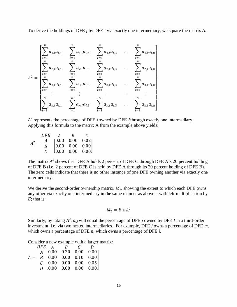
To derive the holdings of DFE j by DFE i via exactly one intermediary, we square the matrix A:

𝐴2 =

[ ∑𝑎1,𝑖𝑎𝑖,1

𝑛

𝑖=1

∑𝑎1,𝑖𝑎𝑖,2

𝑛

𝑖=1

∑𝑎1,𝑖𝑎𝑖,3

𝑛

𝑖=1

… ∑𝑎1,𝑖𝑎𝑖,𝑛

𝑛

𝑖=1

∑𝑎2,𝑖𝑎𝑖,1

𝑛

𝑖=1

∑𝑎2,𝑖𝑎𝑖,2

𝑛

𝑖=1

∑𝑎2,𝑖𝑎𝑖,3

𝑛

𝑖=1

… ∑𝑎2,𝑖𝑎𝑖,𝑛

𝑛

𝑖=1

∑𝑎3,𝑖𝑎𝑖,1

𝑛

𝑖=1

∑𝑎3,𝑖𝑎𝑖,2

𝑛

𝑖=1

∑𝑎3,𝑖𝑎𝑖,3

𝑛

𝑖=1

… ∑𝑎3,𝑖𝑎𝑖,𝑛

𝑛

𝑖=1

⋮ ⋮ ⋮ ⋱ ⋮

∑𝑎𝑛,𝑖𝑎𝑖,1

𝑛

𝑖=1

∑𝑎𝑛,𝑖𝑎𝑖,2

𝑛

𝑖=1

∑𝑎𝑛,𝑖𝑎𝑖,3

𝑛

𝑖=1

… ∑𝑎𝑛,𝑖𝑎𝑖,𝑛

𝑛

𝑖=1 ]

.

A2 represents the percentage of DFE j owned by DFE i through exactly one intermediary.

Applying this formula to the matrix A from the example above yields:

𝐴2 =

𝐷𝐹𝐸𝐴𝐵𝐶

𝐴 𝐵 𝐶

[0.00 0.00 0.020.00 0.00 0.000.00 0.00 0.00

]

The matrix A2 shows that DFE A holds 2 percent of DFE C through DFE A’s 20 percent holding

of DFE B (i.e. 2 percent of DFE C is held by DFE A through its 20 percent holding of DFE B).

The zero cells indicate that there is no other instance of one DFE owning another via exactly one

intermediary.

We derive the second-order ownership matrix, M2, showing the extent to which each DFE owns

any other via exactly one intermediary in the same manner as above – with left multiplication by

E; that is:

𝑀2 = 𝐸 ∗ 𝐴2

Similarly, by taking A3, ai,j will equal the percentage of DFE j owned by DFE I in a third-order

investment, i.e. via two nested intermediaries. For example, DFE j owns a percentage of DFE m,

which owns a percentage of DFE n, which owns a percentage of DFE i.

Consider a new example with a larger matrix:

𝐴 =

𝐷𝐹𝐸𝐴𝐵𝐶𝐷

𝐴 𝐵 𝐶 𝐷

[

0.00 0.20 0.00 0.000.00 0.00 0.10 0.000.00 0.00 0.00 0.050.00 0.00 0.00 0.00

]

16

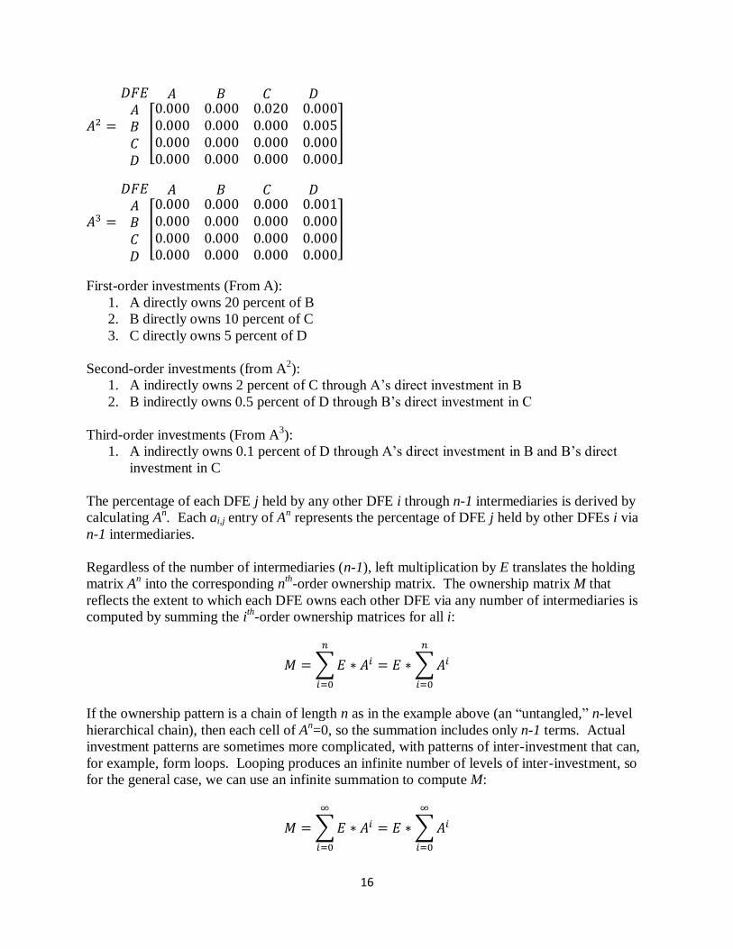
𝐴2 =

𝐷𝐹𝐸𝐴𝐵𝐶𝐷

𝐴 𝐵 𝐶 𝐷

[

0.000 0.000 0.020 0.0000.000 0.000 0.000 0.0050.000 0.000 0.000 0.0000.000 0.000 0.000 0.000

]

𝐴3 =

𝐷𝐹𝐸𝐴𝐵𝐶𝐷

𝐴 𝐵 𝐶 𝐷

[

0.000 0.000 0.000 0.0010.000 0.000 0.000 0.0000.000 0.000 0.000 0.0000.000 0.000 0.000 0.000

]

First-order investments (From A):

1. A directly owns 20 percent of B

2. B directly owns 10 percent of C

3. C directly owns 5 percent of D

Second-order investments (from A2):

1. A indirectly owns 2 percent of C through A’s direct investment in B

2. B indirectly owns 0.5 percent of D through B’s direct investment in C

Third-order investments (From A3):

1. A indirectly owns 0.1 percent of D through A’s direct investment in B and B’s direct

investment in C

The percentage of each DFE j held by any other DFE i through n-1 intermediaries is derived by

calculating An. Each ai,j entry of A

n represents the percentage of DFE j held by other DFEs i via

n-1 intermediaries.

Regardless of the number of intermediaries (n-1), left multiplication by E translates the holding

matrix An into the corresponding n

th-order ownership matrix. The ownership matrix M that

reflects the extent to which each DFE owns each other DFE via any number of intermediaries is

computed by summing the ith

-order ownership matrices for all i:

𝑀 = ∑𝐸 ∗ 𝐴𝑖

𝑛

𝑖=0

= 𝐸 ∗ ∑𝐴𝑖

𝑛

𝑖=0

If the ownership pattern is a chain of length n as in the example above (an “untangled,” n-level

hierarchical chain), then each cell of An=0, so the summation includes only n-1 terms. Actual

investment patterns are sometimes more complicated, with patterns of inter-investment that can,

for example, form loops. Looping produces an infinite number of levels of inter-investment, so

for the general case, we can use an infinite summation to compute M:

𝑀 = ∑𝐸 ∗ 𝐴𝑖

∞

𝑖=0

= 𝐸 ∗ ∑𝐴𝑖

∞

𝑖=0

17

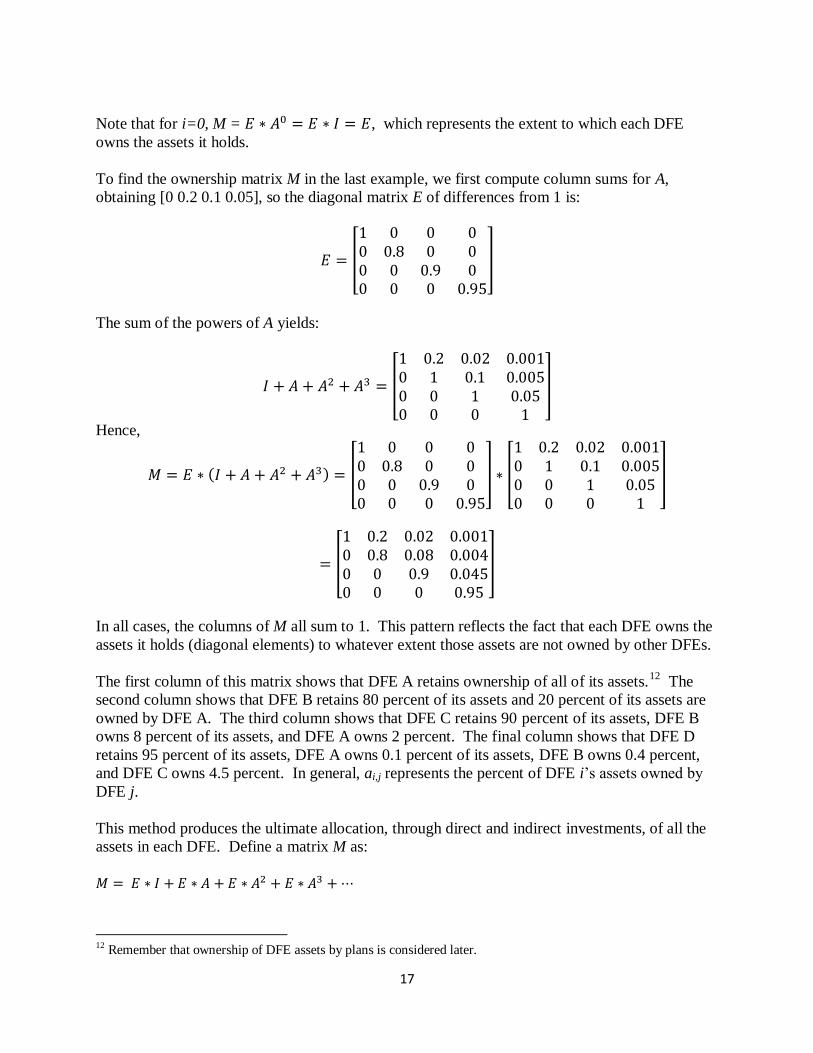
Note that for i=0, M = 𝐸 ∗ 𝐴0 = 𝐸 ∗ 𝐼 = 𝐸, which represents the extent to which each DFE

owns the assets it holds.

To find the ownership matrix M in the last example, we first compute column sums for A,

obtaining [0 0.2 0.1 0.05], so the diagonal matrix E of differences from 1 is:

𝐸 = [

1 0 0 00 0.8 0 00 0 0.9 00 0 0 0.95

]

The sum of the powers of A yields:

𝐼 + 𝐴 + 𝐴2 + 𝐴3 = [

1 0.2 0.02 0.0010 1 0.1 0.0050 0 1 0.050 0 0 1

]

Hence,

𝑀 = 𝐸 ∗ (𝐼 + 𝐴 + 𝐴2 + 𝐴3) = [

1 0 0 00 0.8 0 00 0 0.9 00 0 0 0.95

] ∗ [

1 0.2 0.02 0.0010 1 0.1 0.0050 0 1 0.050 0 0 1

]

= [

1 0.2 0.02 0.0010 0.8 0.08 0.0040 0 0.9 0.0450 0 0 0.95

]

In all cases, the columns of M all sum to 1. This pattern reflects the fact that each DFE owns the

assets it holds (diagonal elements) to whatever extent those assets are not owned by other DFEs.

The first column of this matrix shows that DFE A retains ownership of all of its assets.12

The

second column shows that DFE B retains 80 percent of its assets and 20 percent of its assets are

owned by DFE A. The third column shows that DFE C retains 90 percent of its assets, DFE B

owns 8 percent of its assets, and DFE A owns 2 percent. The final column shows that DFE D

retains 95 percent of its assets, DFE A owns 0.1 percent of its assets, DFE B owns 0.4 percent,

and DFE C owns 4.5 percent. In general, ai,j represents the percent of DFE i’s assets owned by

DFE j.

This method produces the ultimate allocation, through direct and indirect investments, of all the

assets in each DFE. Define a matrix M as:

𝑀 = 𝐸 ∗ 𝐼 + 𝐸 ∗ 𝐴 + 𝐸 ∗ 𝐴2 + 𝐸 ∗ 𝐴3 + ⋯

12 Remember that ownership of DFE assets by plans is considered later.

18

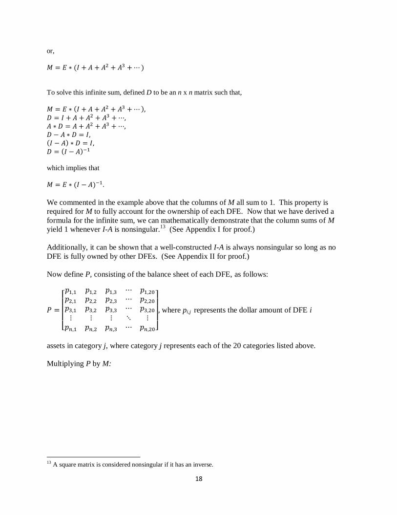
or,

𝑀 = 𝐸 ∗ (𝐼 + 𝐴 + 𝐴2 + 𝐴3 + ⋯)

To solve this infinite sum, defined D to be an n x n matrix such that,

𝑀 = 𝐸 ∗ (𝐼 + 𝐴 + 𝐴2 + 𝐴3 + ⋯), 𝐷 = 𝐼 + 𝐴 + 𝐴2 + 𝐴3 + ⋯, 𝐴 ∗ 𝐷 = 𝐴 + 𝐴2 + 𝐴3 + ⋯, 𝐷 − 𝐴 ∗ 𝐷 = 𝐼, (𝐼 − 𝐴) ∗ 𝐷 = 𝐼, 𝐷 = (𝐼 − 𝐴)−1

which implies that

𝑀 = 𝐸 ∗ (𝐼 − 𝐴)−1.

We commented in the example above that the columns of M all sum to 1. This property is

required for M to fully account for the ownership of each DFE. Now that we have derived a

formula for the infinite sum, we can mathematically demonstrate that the column sums of M

yield 1 whenever I-A is nonsingular.13

(See Appendix I for proof.)

Additionally, it can be shown that a well-constructed I-A is always nonsingular so long as no

DFE is fully owned by other DFEs. (See Appendix II for proof.)

Now define P, consisting of the balance sheet of each DFE, as follows:

𝑃 =

[ 𝑝1,1 𝑝1,2 𝑝1,3 ⋯ 𝑝1,20

𝑝2,1 𝑝2,2 𝑝2,3 ⋯ 𝑝2,20

𝑝3,1 𝑝3,2 𝑝3,3 ⋯ 𝑝3,20

⋮ ⋮ ⋮ ⋱ ⋮𝑝𝑛,1 𝑝𝑛,2 𝑝𝑛,3 ⋯ 𝑝𝑛,20]

, where pi,j represents the dollar amount of DFE i

assets in category j, where category j represents each of the 20 categories listed above.

Multiplying P by M:

13 A square matrix is considered nonsingular if it has an inverse.

19

𝐵 = 𝑀 ∗ 𝑃 =

[ ∑𝑚1,𝑖𝑝𝑖,1

𝑛

𝑖=1

∑𝑚1,𝑖𝑝𝑖,2

𝑛

𝑖=1

∑ 𝑚1,𝑖𝑝𝑖,3

𝑛

𝑖=1

… ∑𝑚1,𝑖𝑝𝑖,20

𝑛

𝑖=1

∑𝑚2,𝑖𝑝𝑖,1

𝑛

𝑖=1

∑ 𝑚2,𝑖𝑝𝑖,2

𝑛

𝑖=1

∑ 𝑚2,𝑖𝑝𝑖,3

𝑛

𝑖=1

… ∑𝑚2,𝑖𝑝𝑖,20

𝑛

𝑖=1

∑𝑚3,𝑖𝑝𝑖,1

𝑛

𝑖=1

∑ 𝑚3,𝑖𝑝𝑖,2

𝑛

𝑖=1

∑ 𝑚3,𝑖𝑝𝑖,3

𝑛

𝑖=1

… ∑𝑚3,𝑖𝑝𝑖,20

𝑛

𝑖=1

⋮ ⋮ ⋮ ⋱ ⋮

∑𝑚𝑛,𝑖𝑝𝑖,1

𝑛

𝑖=1

∑ 𝑚𝑛,𝑖𝑝𝑖,2

𝑛

𝑖=1

∑ 𝑚𝑛,𝑖𝑝𝑖,3

𝑛

𝑖=1

… ∑𝑚𝑛,𝑖𝑝𝑖,20

𝑛

𝑖=1 ]

This matrix multiplication produces an n x 20 matrix B where each bi,j represents the dollars in

each asset category j owned by DFE i or held by DFE i and not reported as being owned by any

other DFEs. Row i of this matrix therefore reports the asset allocation of DFE i that will be used

in spreading pension assets.

VI. Application of Matrix Algebra

The discussion of matrix algebra above explains the theoretical framework used to derive the

‘spread allocation’ for DFEs. However, this discussion does not take into account the impact of

missing data. Therefore, as discussed earlier, a ‘closed’ DFE set is created. This dataset consists

of all DFEs that are completely unaffected by missing data, either directly or indirectly. This

‘closed’ set is created as follows. First, a matrix A is created exactly as described above.

𝐴 =

[ 𝑎1,1 𝑎1,2 𝑎1,3 … 𝑎1,𝑛

𝑎2,1 𝑎2,2 𝑎2,3 … 𝑎2,𝑛

𝑎3,1 𝑎3,2 𝑎3,3 … 𝑎3,𝑛

⋮ ⋮ ⋮ ⋱ ⋮𝑎𝑛,1 𝑎𝑛,2 𝑎𝑛,3 … 𝑎𝑛,𝑛]

, 𝑤ℎ𝑒𝑟𝑒 𝑎𝑖,𝑗 =𝐷𝐹𝐸 𝑖 𝑖𝑛𝑣𝑒𝑠𝑡𝑚𝑒𝑛𝑡 𝑖𝑛 𝐷𝐹𝐸 𝑗

𝐷𝐹𝐸 𝑗 𝑡𝑜𝑡𝑎𝑙 𝑎𝑠𝑠𝑒𝑡𝑠

This matrix is then altered in one simple fashion. An additional row and column is added as

follows:

𝐴 =

[ 𝑎1,1 𝑎1,2 𝑎1,3 … 𝑎1,𝑛 𝑏1,𝑚𝑖𝑠𝑠𝑖𝑛𝑔

𝑎2,1 𝑎2,2 𝑎2,3 … 𝑎2,𝑛 𝑏2,𝑚𝑖𝑠𝑠𝑖𝑛𝑔

𝑎3,1 𝑎3,2 𝑎3,3 … 𝑎3,𝑛 𝑏2,𝑚𝑖𝑠𝑠𝑖𝑛𝑔

⋮ ⋮ ⋮ ⋱ ⋮ ⋮𝑎𝑛,1 𝑎𝑛,2 𝑎𝑛,3 … 𝑎𝑛,𝑛 𝑏𝑛,𝑚𝑖𝑠𝑠𝑖𝑛𝑔

0 0 0 0 0 0 ]

, 𝑤ℎ𝑒𝑟𝑒 𝑎𝑖,𝑗 =𝐷𝐹𝐸 𝑖 𝑖𝑛𝑣𝑒𝑠𝑡𝑚𝑒𝑛𝑡 𝑖𝑛 𝐷𝐹𝐸 𝑗

𝐷𝐹𝐸 𝑗 𝑡𝑜𝑡𝑎𝑙 𝑎𝑠𝑠𝑒𝑡𝑠 𝑎𝑛𝑑

𝑏𝑖,𝑚𝑖𝑠𝑠𝑖𝑛𝑔 = 𝑆𝑢𝑚 𝑜𝑓 𝐷𝐹𝐸 𝑖 𝑖𝑛𝑣𝑒𝑠𝑡𝑚𝑒𝑛𝑡 𝑖𝑛 𝐷𝐹𝐸𝑠 𝑛𝑜𝑡 𝑟𝑒𝑝𝑟𝑒𝑠𝑒𝑛𝑡𝑒𝑑 𝑖𝑛 𝑑𝑎𝑡𝑎𝑠𝑒𝑡 (𝑛𝑜𝑡 𝑖𝑛 𝑛)

Once this matrix is created, the ownership matrix M is calculated as

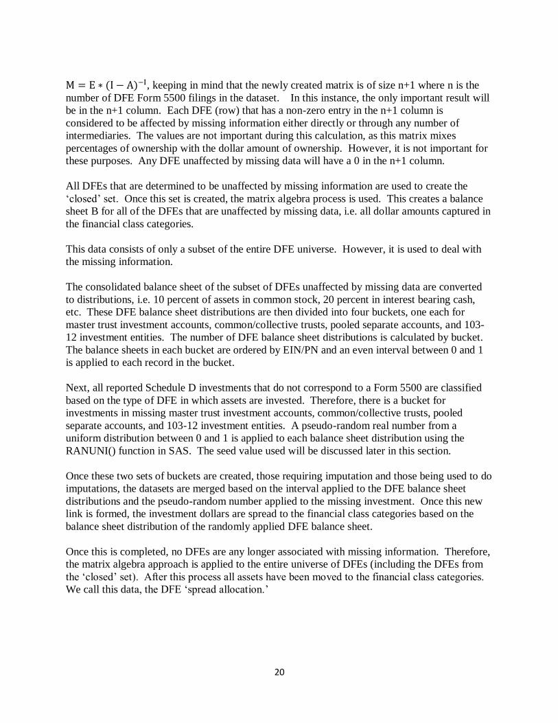
20

M = E ∗ (I − A)−I, keeping in mind that the newly created matrix is of size n+1 where n is the

number of DFE Form 5500 filings in the dataset. In this instance, the only important result will

be in the n+1 column. Each DFE (row) that has a non-zero entry in the n+1 column is

considered to be affected by missing information either directly or through any number of

intermediaries. The values are not important during this calculation, as this matrix mixes

percentages of ownership with the dollar amount of ownership. However, it is not important for

these purposes. Any DFE unaffected by missing data will have a 0 in the n+1 column.

All DFEs that are determined to be unaffected by missing information are used to create the

‘closed’ set. Once this set is created, the matrix algebra process is used. This creates a balance

sheet B for all of the DFEs that are unaffected by missing data, i.e. all dollar amounts captured in

the financial class categories.

This data consists of only a subset of the entire DFE universe. However, it is used to deal with

the missing information.

The consolidated balance sheet of the subset of DFEs unaffected by missing data are converted

to distributions, i.e. 10 percent of assets in common stock, 20 percent in interest bearing cash,

etc. These DFE balance sheet distributions are then divided into four buckets, one each for

master trust investment accounts, common/collective trusts, pooled separate accounts, and 103-

12 investment entities. The number of DFE balance sheet distributions is calculated by bucket.

The balance sheets in each bucket are ordered by EIN/PN and an even interval between 0 and 1

is applied to each record in the bucket.

Next, all reported Schedule D investments that do not correspond to a Form 5500 are classified

based on the type of DFE in which assets are invested. Therefore, there is a bucket for

investments in missing master trust investment accounts, common/collective trusts, pooled

separate accounts, and 103-12 investment entities. A pseudo-random real number from a

uniform distribution between 0 and 1 is applied to each balance sheet distribution using the

RANUNI() function in SAS. The seed value used will be discussed later in this section.

Once these two sets of buckets are created, those requiring imputation and those being used to do

imputations, the datasets are merged based on the interval applied to the DFE balance sheet

distributions and the pseudo-random number applied to the missing investment. Once this new

link is formed, the investment dollars are spread to the financial class categories based on the

balance sheet distribution of the randomly applied DFE balance sheet.

Once this is completed, no DFEs are any longer associated with missing information. Therefore,

the matrix algebra approach is applied to the entire universe of DFEs (including the DFEs from

the ‘closed’ set). After this process all assets have been moved to the financial class categories.

We call this data, the DFE ‘spread allocation.’

21

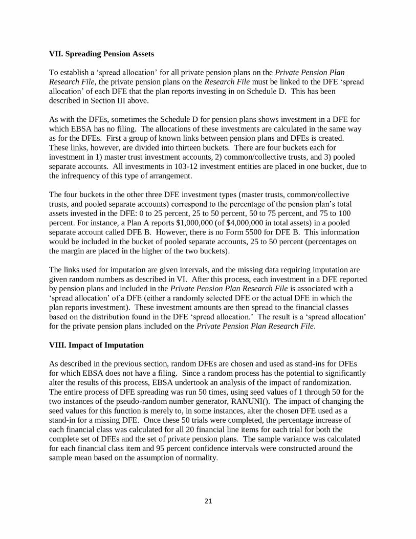
VII. Spreading Pension Assets

To establish a ‘spread allocation’ for all private pension plans on the Private Pension Plan

Research File, the private pension plans on the Research File must be linked to the DFE ‘spread

allocation’ of each DFE that the plan reports investing in on Schedule D. This has been

described in Section III above.

As with the DFEs, sometimes the Schedule D for pension plans shows investment in a DFE for

which EBSA has no filing. The allocations of these investments are calculated in the same way

as for the DFEs. First a group of known links between pension plans and DFEs is created.

These links, however, are divided into thirteen buckets. There are four buckets each for

investment in 1) master trust investment accounts, 2) common/collective trusts, and 3) pooled

separate accounts. All investments in 103-12 investment entities are placed in one bucket, due to

the infrequency of this type of arrangement.

The four buckets in the other three DFE investment types (master trusts, common/collective

trusts, and pooled separate accounts) correspond to the percentage of the pension plan’s total

assets invested in the DFE: 0 to 25 percent, 25 to 50 percent, 50 to 75 percent, and 75 to 100

percent. For instance, a Plan A reports $1,000,000 (of $4,000,000 in total assets) in a pooled

separate account called DFE B. However, there is no Form 5500 for DFE B. This information

would be included in the bucket of pooled separate accounts, 25 to 50 percent (percentages on

the margin are placed in the higher of the two buckets).

The links used for imputation are given intervals, and the missing data requiring imputation are

given random numbers as described in VI. After this process, each investment in a DFE reported

by pension plans and included in the Private Pension Plan Research File is associated with a

‘spread allocation’ of a DFE (either a randomly selected DFE or the actual DFE in which the

plan reports investment). These investment amounts are then spread to the financial classes

based on the distribution found in the DFE ‘spread allocation.’ The result is a ‘spread allocation’

for the private pension plans included on the Private Pension Plan Research File.

VIII. Impact of Imputation

As described in the previous section, random DFEs are chosen and used as stand-ins for DFEs

for which EBSA does not have a filing. Since a random process has the potential to significantly

alter the results of this process, EBSA undertook an analysis of the impact of randomization.

The entire process of DFE spreading was run 50 times, using seed values of 1 through 50 for the

two instances of the pseudo-random number generator, RANUNI(). The impact of changing the

seed values for this function is merely to, in some instances, alter the chosen DFE used as a

stand-in for a missing DFE. Once these 50 trials were completed, the percentage increase of

each financial class was calculated for all 20 financial line items for each trial for both the

complete set of DFEs and the set of private pension plans. The sample variance was calculated

for each financial class item and 95 percent confidence intervals were constructed around the

sample mean based on the assumption of normality.

22

The following charts show the mean, confidence intervals, and the results of a single trial for the

set of all DFEs and the spread Private Pension Plan Bulletin. By being able to review each

individual trial in comparison to the average and variance of all the trials, EBSA was able to

choose a trial that seemed representative of all trials, in which the increase to a particular

financial class line item was not an outlier. Additionally, by reviewing the width of the

confidence intervals for each variable, EBSA was able to feel confident that the result of any

random imputation would not be large on the final results of this project.

23

-2%

-1%

0%

1%

2%

3%

4%

5%

6%

7%

8%

9%

Sample Mean, 95% Confidence Intervals, and Individual Data Points for Percentage Changes Due to Spreading for DFEs

Mean

Upper CL 95%

Lower CL 95%

sample value

24

0%

100%

200%

300%

400%

500%

600%

700%

800%

900%

Sample Mean, 95% Confidence Intervals, and Individual Data Points for Percentage Changes Due to Spreading for Plans

Mean

Upper CL 95%

Lower CL 95%

sample value

25

Technical Appendix I

The column sums of 𝑀 = 𝐸 ∗ (𝐼 − 𝐴)−1 are 1 if 𝐼 − 𝐴 is nonsingular.

Proof:

Let 𝐽 be an n x 1 column vector of all 1’s, and let 𝑊 be an n x n matrix, then 𝐽𝑡 ∗ 𝑊 yields a row

vector with entries equal to the sum of the columns of 𝑊. We can therefore express the vector

with entries equal to the sum of the columns of 𝐸 ∗ (1 − 𝐴)−1 as:

𝐽𝑡 ∗ (𝐸 ∗ (1 − 𝐴)−1)

The matrix E can be written as 𝐼 − 𝑑𝑖𝑎𝑔(𝐽𝑡 ∗ 𝐴). (The notation 𝑑𝑖𝑎𝑔(𝑣) represents the diagonal

matrix whose i,i element is vi.) Therefore,

𝐽𝑡 ∗ (𝐸 ∗ (1 − 𝐴)−1) = 𝐽𝑡 ∗ ((𝐼 − 𝑑𝑖𝑎𝑔(𝐽𝑡 ∗ 𝐴)) ∗ (𝐼 − 𝐴)−1) Expressing I as a diagonal matrix of its own column sums, we can write:

= 𝐽𝑡 ∗ ((𝑑𝑖𝑎𝑔(𝐽𝑡 ∗ 𝐼) − 𝑑𝑖𝑎𝑔(𝐽𝑡 ∗ 𝐴)) ∗ (𝐼 − 𝐴)−1)

Because a difference of diagonal matrices is the diagonal matrix of the differences:

= 𝐽𝑡 ∗ (𝑑𝑖𝑎𝑔(𝐽𝑡 ∗ 𝐼 − 𝐽𝑡 ∗ 𝐴) ∗ (𝐼 − 𝐴)−1)

Factoring:

= 𝐽𝑡 ∗ (𝑑𝑖𝑎𝑔(𝐽𝑡 ∗ (𝐼 − 𝐴)) ∗ (𝐼 − 𝐴)−1)

By associativity:

= (𝐽𝑡 ∗ 𝑑𝑖𝑎𝑔(𝐽𝑡 ∗ (𝐼 − 𝐴))) ∗ (𝐼 − 𝐴)−1

For any vector v, 𝐽𝑡 ∗ 𝑑𝑖𝑎𝑔(𝑣) = 𝑣, hence:

= (𝐽𝑡 ∗ (𝐼 − 𝐴)) ∗ (𝐼 − 𝐴)−1

Again by associativity:

= 𝐽𝑡 ∗ ((𝐼 − 𝐴) ∗ (𝐼 − 𝐴)−1)

= 𝐽𝑡 ∗ 𝐼

= 𝐽𝑡

So we have shown that the vector with entries equal to the sum of the columns of 𝐸 ∗ (𝐼 − 𝐴)−1

equals 𝐽𝑡, the vector consisting of all ones, hence columns of 𝐸 ∗ (𝐼 − 𝐴)−1 sum to one when

𝐼 − 𝐴 has an inverse.

EBSA appreciates the mathematical assistance with this proof provided by George Washington

University Associate Professor Lowell Abrams.

26

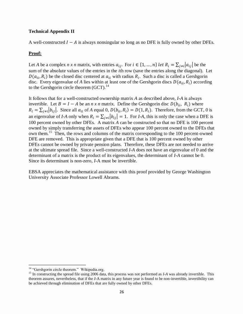
Technical Appendix II

A well-constructed 𝐼 − 𝐴 is always nonsingular so long as no DFE is fully owned by other DFEs.

Proof:

Let A be a complex n x n matrix, with entries 𝑎𝑖𝑗 . For 𝑖 ∈ {1,… , 𝑛} 𝑙𝑒𝑡 𝑅𝑖 = ∑ |𝑎𝑖𝑗|𝑗≠𝑖 be the

sum of the absolute values of the entries in the ith row (save the entries along the diagonal). Let

𝐷(𝑎𝑖𝑖 , 𝑅𝑖) be the closed disc centered at 𝑎𝑖𝑖 with radius 𝑅𝑖. Such a disc is called a Gershgorin

disc. Every eigenvalue of A lies within at least one of the Gershgorin discs 𝐷(𝑎𝑖𝑖, 𝑅𝑖) according

to the Gershgorin circle theorem (GCT).14

It follows that for a well-constructed ownership matrix A as described above, I-A is always

invertible. Let 𝐵 = 𝐼 − 𝐴 be an n x n matrix. Define the Gershgorin disc 𝐷(𝑏𝑖𝑖 , 𝑅𝑖) where

𝑅𝑖 = ∑ |𝑏𝑖𝑗|𝑗≠𝑖 . Since all 𝑎𝑖𝑖 of A equal 0, 𝐷(𝑏𝑖𝑖 , 𝑅𝑖) = 𝐷(1, 𝑅𝑖). Therefore, from the GCT, 0 is

an eigenvalue of I-A only when 𝑅𝑖 = ∑ |𝑏𝑖𝑗|𝑗≠𝑖 = 1. For I-A, this is only the case when a DFE is

100 percent owned by other DFEs. A matrix A can be constructed so that no DFE is 100 percent

owned by simply transferring the assets of DFEs who appear 100 percent owned to the DFEs that

own them.15

Then, the rows and columns of the matrix corresponding to the 100 percent-owned

DFE are removed. This is appropriate given that a DFE that is 100 percent owned by other

DFEs cannot be owned by private pension plans. Therefore, these DFEs are not needed to arrive

at the ultimate spread file. Since a well-constructed I-A does not have an eigenvalue of 0 and the

determinant of a matrix is the product of its eigenvalues, the determinant of I-A cannot be 0.

Since its determinant is non-zero, I-A must be invertible.

EBSA appreciates the mathematical assistance with this proof provided by George Washington

University Associate Professor Lowell Abrams.

14 “Gershgorin circle theorem.” Wikipedia.org. 15 In constructing the spread file using 2006 data, this process was not performed as I-A was already invertible. This

theorem assures, nevertheless, that if the I-A matrix in any future year is found to be non-invertible, invertibility can

be achieved through elimination of DFEs that are fully owned by other DFEs.