Embed Size (px)
Citation preview
General rights Copyright and moral rights for the publications made accessible in the public portal are retained by the authors and/or other copyright owners and it is a condition of accessing publications that users recognise and abide by the legal requirements associated with these rights.
Users may download and print one copy of any publication from the public portal for the purpose of private study or research.
You may not further distribute the material or use it for any profit-making activity or commercial gain
You may freely distribute the URL identifying the publication in the public portal If you believe that this document breaches copyright please contact us providing details, and we will remove access to the work immediately and investigate your claim.
Downloaded from orbit.dtu.dk on: Apr 16, 2020
User’s Manual for BECASA cross section analysis tool for anisotropic and inhomogeneous beam sections of arbitrarygeometryBlasques, José Pedro Albergaria Amaral
Publication date:2012
Document VersionPublisher's PDF, also known as Version of record
Link back to DTU Orbit
Citation (APA):Blasques, J. P. A. A. (2012). User’s Manual for BECAS: A cross section analysis tool for anisotropic andinhomogeneous beam sections of arbitrary geometry. Risø DTU – National Laboratory for Sustainable Energy.Denmark. Forskningscenter Risoe. Risoe-R, No. 1785(EN)
User’s Manual for
BECAS
A cross section analysis tool for anisotropic and inhomogeneous
beam sections of arbitrary geometry
Jose Pedro BlasquesRisø DTU – National Laboratory for Sustainable Energy
Technical University of DenmarkFrederiksborgvej 399, P.O. Box 49, Building 114,
DK-4000 Roskilde, Denmark� [email protected]
RISØ-R 1785
February 23, 2012
c© Risø DTU – National Laboratory for Sustainable Energy

ii
Title of report:User’s Manual for BECAS v2.0 - a cross section analysis tool for anisotropic andinhomogeneous beam sections of arbitrary geometry
Author:Jose Pedro BlasquesAddress: Risø – National Laboratory for Sustainable EnergyTechnical University of DenmarkFrederiksborgvej 399, P.O. Box 49, Building 114,DK-4000 Roskilde, DenmarkE-mail: [email protected]
Copyright and ownership:All rights to this User’s Manual belong exclusively to Risø DTU. This User’s Man-ual may only be accessed when the reader has a valid license from Risø DTU touse the BECAS software. A license can be obtained from Jose Pedro Blasques [email protected].
Disclaimer:Risø DTU disclaims all responsibility for any kind of damage, including loss of profit,loss of capital or any caused damage or loss, which might appear by use or erroneoususe of the BECAS software or Documentation, even though Risø DTU should havebeen informed of the possibilities of such damage.
iii

iv
Preface
The BEam Cross section Analysis Software - BECAS - is a group of Matlab functionsused for the analysis of the stiffness and mass properties of beam cross sections. BE-CAS was originally developed under the EFP 2007 Project 33033-0075 - Anisotropicbeam model for analysis and design of passive controlled wind turbine blades. BE-CAS was later updated, extended, and completely rewritten throughout part ofthe author’s Ph.D. project (Optimal Design of Laminated Composite Beams, Ph.D.Thesis, Technical University of Denmark).
BECAS’ code and user’s guide is mostly developed and maintained by Jose PedroBlasques (Risø DTU, National Laboratory for Sustainable Energy, TechnicalUniversity of Denmark). Nonetheless, the author is indebted to the followingpeople which at one point or another have given or currently give invaluablesupport throughout the development of BECAS:
• Boyan Lazarov (Department of Mechanical Engineering, Technical Universityof Denmark) Participated very actively in the development of the originalBECAS v1.0. Among much other invaluable work, Boyan was the first tosuggest the constraint equations which are used in the solution of the crosssection equilibrium equations.
• Robert Bitsche (Risø DTU, National Laboratory for Sustainable Energy,Technical University of Denmark) An active member of the current BECASdevelopment group. Robert is the main bug finder, and an invaluable sourceof good ideas and suggestions. Robert is also responsible for the interfacebetween BECAS, commercial finite element packages, and HAWC2, RisøDTU’s own code for the aeroelastic analysis of wind turbines.
Their contributions are gratefully acknowledged.
All feedback and suggestions for further improvements and extensions is mostwelcome.
Jose Pedro Blasques
Roskilde, November 2011
v

vi PREFACE
Contents
Preface v
1 Introduction 1
1.1 Version history . . . . . . . . . . . . . . . . . . . . . . . . . . . . . . 3
2 Theory manual 5
2.1 Assumptions . . . . . . . . . . . . . . . . . . . . . . . . . . . . . . . 5
2.2 Equilibrium equations . . . . . . . . . . . . . . . . . . . . . . . . . . 6
2.2.1 Basic definitions . . . . . . . . . . . . . . . . . . . . . . . . . 6
2.2.2 Kinematics . . . . . . . . . . . . . . . . . . . . . . . . . . . . 7
2.2.3 Strain-displacement relation . . . . . . . . . . . . . . . . . . . 8
2.2.4 Virtual work principle . . . . . . . . . . . . . . . . . . . . . . 9
2.3 Solutions to equilibrium equations . . . . . . . . . . . . . . . . . . . 13
2.3.1 Extremity solutions . . . . . . . . . . . . . . . . . . . . . . . 13
2.3.2 Central solutions . . . . . . . . . . . . . . . . . . . . . . . . . 14
2.3.3 Constraint equations . . . . . . . . . . . . . . . . . . . . . . . 16
2.4 On the properties of the solutions . . . . . . . . . . . . . . . . . . . . 16
2.4.1 Rigid motions . . . . . . . . . . . . . . . . . . . . . . . . . . . 17
2.4.2 Warping displacements . . . . . . . . . . . . . . . . . . . . . . 19
2.5 Cross section properties . . . . . . . . . . . . . . . . . . . . . . . . . 22
2.5.1 Cross section stiffness matrix . . . . . . . . . . . . . . . . . . 22
2.5.2 Shear center and elastic center positions . . . . . . . . . . . . 24
2.6 Cross section mass matrix . . . . . . . . . . . . . . . . . . . . . . . . 25
2.7 An alternative formulation based on solid finite elements . . . . . . . 26
2.7.1 Evaluation of cross section stiffness matrix . . . . . . . . . . . 26
3 Implementation manual 29
3.1 Two dimensional finite element analysis . . . . . . . . . . . . . . . . 29
3.1.1 Q4 and Q8 elements . . . . . . . . . . . . . . . . . . . . . . . 29
3.1.2 Local and global finite element matrices . . . . . . . . . . . . 32
3.2 Material constitutive matrix . . . . . . . . . . . . . . . . . . . . . . . 33
3.2.1 Definition . . . . . . . . . . . . . . . . . . . . . . . . . . . . . 33
3.2.2 Rotation . . . . . . . . . . . . . . . . . . . . . . . . . . . . . . 34
3.3 Rotation and translation of constitutive matrices . . . . . . . . . . . 36
vii
viii CONTENTS
4 Validation 374.1 Setup . . . . . . . . . . . . . . . . . . . . . . . . . . . . . . . . . . . 374.2 Numerical examples . . . . . . . . . . . . . . . . . . . . . . . . . . . 40
4.2.1 Square . . . . . . . . . . . . . . . . . . . . . . . . . . . . . . . 414.2.2 Cylinder . . . . . . . . . . . . . . . . . . . . . . . . . . . . . . 504.2.3 Three cells . . . . . . . . . . . . . . . . . . . . . . . . . . . . 60
5 User’s Manual 655.1 Input . . . . . . . . . . . . . . . . . . . . . . . . . . . . . . . . . . . . 66
5.1.1 Example . . . . . . . . . . . . . . . . . . . . . . . . . . . . . . 675.2 List of functions and output . . . . . . . . . . . . . . . . . . . . . . . 67
5.2.1 BECAS_Utils . . . . . . . . . . . . . . . . . . . . . . . . . . . 675.2.2 BECAS_Constitutive_Ks . . . . . . . . . . . . . . . . . . . . 675.2.3 BECAS_Constitutive_Ms . . . . . . . . . . . . . . . . . . . . 675.2.4 BECAS_CrossSectionProps . . . . . . . . . . . . . . . . . . . 685.2.5 BECAS_RecoverStrains . . . . . . . . . . . . . . . . . . . . . 695.2.6 BECAS_RecoverStresses . . . . . . . . . . . . . . . . . . . . 695.2.7 BECAS_Becas2Hawc2 . . . . . . . . . . . . . . . . . . . . . . . 705.2.8 BECAS_TransformMat . . . . . . . . . . . . . . . . . . . . . . 705.2.9 Examples . . . . . . . . . . . . . . . . . . . . . . . . . . . . . 71
5.3 The BECAS 3D implementation . . . . . . . . . . . . . . . . . . . . 715.3.1 Input . . . . . . . . . . . . . . . . . . . . . . . . . . . . . . . 715.3.2 List of functions and output . . . . . . . . . . . . . . . . . . . 715.3.3 BECAS_3D_Utils . . . . . . . . . . . . . . . . . . . . . . . . . 715.3.4 BECAS_3D_Constitutive_Ks . . . . . . . . . . . . . . . . . . 725.3.5 BECAS_3D_CrossSectionProps . . . . . . . . . . . . . . . . . 72
List of Symbols
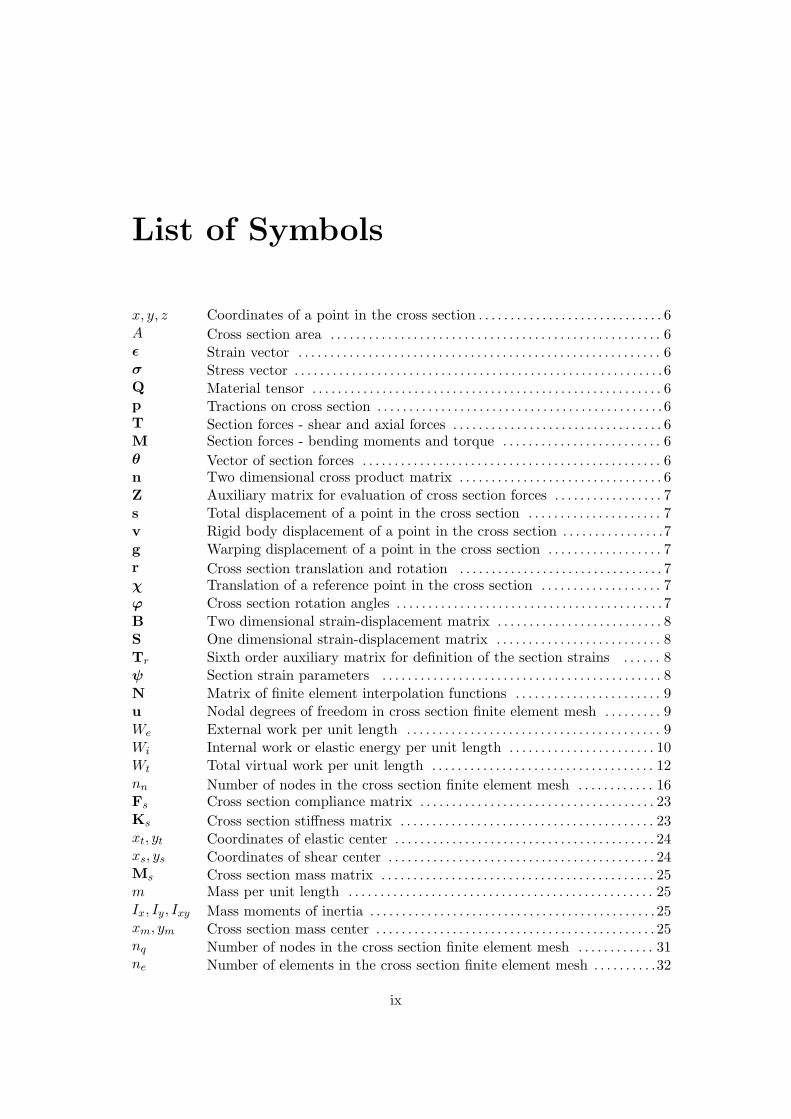
x, y, z Coordinates of a point in the cross section . . . . . . . . . . . . . . . . . . . . . . . . . . . . . 6A Cross section area . . . . . . . . . . . . . . . . . . . . . . . . . . . . . . . . . . . . . . . . . . . . . . . . . . . . 6ǫ Strain vector . . . . . . . . . . . . . . . . . . . . . . . . . . . . . . . . . . . . . . . . . . . . . . . . . . . . . . . . . 6σ Stress vector . . . . . . . . . . . . . . . . . . . . . . . . . . . . . . . . . . . . . . . . . . . . . . . . . . . . . . . . . . 6Q Material tensor . . . . . . . . . . . . . . . . . . . . . . . . . . . . . . . . . . . . . . . . . . . . . . . . . . . . . . . 6p Tractions on cross section . . . . . . . . . . . . . . . . . . . . . . . . . . . . . . . . . . . . . . . . . . . . . 6T Section forces - shear and axial forces . . . . . . . . . . . . . . . . . . . . . . . . . . . . . . . . . 6M Section forces - bending moments and torque . . . . . . . . . . . . . . . . . . . . . . . . . 6θ Vector of section forces . . . . . . . . . . . . . . . . . . . . . . . . . . . . . . . . . . . . . . . . . . . . . . . 6n Two dimensional cross product matrix . . . . . . . . . . . . . . . . . . . . . . . . . . . . . . . . 6Z Auxiliary matrix for evaluation of cross section forces . . . . . . . . . . . . . . . . . 7s Total displacement of a point in the cross section . . . . . . . . . . . . . . . . . . . . . 7v Rigid body displacement of a point in the cross section . . . . . . . . . . . . . . . .7g Warping displacement of a point in the cross section . . . . . . . . . . . . . . . . . . 7r Cross section translation and rotation . . . . . . . . . . . . . . . . . . . . . . . . . . . . . . . . 7χ Translation of a reference point in the cross section . . . . . . . . . . . . . . . . . . . 7ϕ Cross section rotation angles . . . . . . . . . . . . . . . . . . . . . . . . . . . . . . . . . . . . . . . . . . 7B Two dimensional strain-displacement matrix . . . . . . . . . . . . . . . . . . . . . . . . . . 8S One dimensional strain-displacement matrix . . . . . . . . . . . . . . . . . . . . . . . . . . 8Tr Sixth order auxiliary matrix for definition of the section strains . . . . . . 8ψ Section strain parameters . . . . . . . . . . . . . . . . . . . . . . . . . . . . . . . . . . . . . . . . . . . . 8N Matrix of finite element interpolation functions . . . . . . . . . . . . . . . . . . . . . . . 9u Nodal degrees of freedom in cross section finite element mesh . . . . . . . . . 9We External work per unit length . . . . . . . . . . . . . . . . . . . . . . . . . . . . . . . . . . . . . . . . 9Wi Internal work or elastic energy per unit length . . . . . . . . . . . . . . . . . . . . . . . 10Wt Total virtual work per unit length . . . . . . . . . . . . . . . . . . . . . . . . . . . . . . . . . . . 12nn Number of nodes in the cross section finite element mesh . . . . . . . . . . . . 16Fs Cross section compliance matrix . . . . . . . . . . . . . . . . . . . . . . . . . . . . . . . . . . . . . 23Ks Cross section stiffness matrix . . . . . . . . . . . . . . . . . . . . . . . . . . . . . . . . . . . . . . . . 23xt, yt Coordinates of elastic center . . . . . . . . . . . . . . . . . . . . . . . . . . . . . . . . . . . . . . . . . 24xs, ys Coordinates of shear center . . . . . . . . . . . . . . . . . . . . . . . . . . . . . . . . . . . . . . . . . . 24Ms Cross section mass matrix . . . . . . . . . . . . . . . . . . . . . . . . . . . . . . . . . . . . . . . . . . . 25m Mass per unit length . . . . . . . . . . . . . . . . . . . . . . . . . . . . . . . . . . . . . . . . . . . . . . . . 25Ix, Iy, Ixy Mass moments of inertia . . . . . . . . . . . . . . . . . . . . . . . . . . . . . . . . . . . . . . . . . . . . . 25xm, ym Cross section mass center . . . . . . . . . . . . . . . . . . . . . . . . . . . . . . . . . . . . . . . . . . . . 25nq Number of nodes in the cross section finite element mesh . . . . . . . . . . . . 31ne Number of elements in the cross section finite element mesh . . . . . . . . . .32
ix

x CONTENTS
nd Number of d.o.f. in the cross section finite element equations . . . . . . . . 67
Chapter 1
Introduction
This report describes the development and implementation of the BEam Crosssection Analysis Software – BECAS.
Cross section analysis tools are commonly employed in the development of beammodels for the analysis of long slender structures. These type of models can be veryversatile when compared against its equivalent counterparts as they generally offer avery good compromise between accuracy and computational efficiency. When suited,beam models can be advantageously used in an optimal design context (see, e.g.,Ganguli and Chopra [1], Li et al. [2], Blasques and Stolpe [3]) or in the developmentof complex multiphysics codes. Wind turbine aeroelastic codes, for example, com-monly rely on these types of models for the representation of most parts of the windturbine, from the tower to the blades (see, e.g., Hansen et al. [4], Chaviaropoulos etal. [5]). In specific, the development of beam models which correctly describe thebehaviour of the wind turbine blades have been the focus of many investigations.The estimation of the properties of these types of structures becomes more complexas the use of different combinations of advanced materials becomes a standard. Itis therefore paramount to develop cross section analysis tools which can correctlyaccount for all geometrical and material effects. BECAS is a general purpose crosssection analysis tool specifically developed for these types of applications. BECASis able to handle a large range of arbitrary section geometries and correctly predictthe effects of inhomogeneous material distribution and anisotropy. Based on a def-inition of the cross section geometry and material distribution, BECAS is able todetermine the cross section stiffness properties while accounting for all the geometri-cal and material induced couplings. These properties can be consequently utilized inthe development of beam models to accurately predict the response of wind turbineblades with complex geometries and made of advanced materials.
BECAS is based on the theory originally presented by Giavotto et al. [6] for theanalysis of inhomogeneous anisotropic beams. The theory leads to the definition oftwo types of solutions of which, and in accordance to Saint-Venant’s principle, thenon-decaying solutions are the basis for the evaluation of the cross section stiffnessproperties. A slight modification to the theory was introduced later by Borri andMerlini [7] where the concept of intrinsic warping is introduced in the derivationof the cross section stiffness matrix. Despite the modifications, no difference in theresults was reported. The theory was subsequently extended by Borri et al [8] toaccount for large displacements, curvature and twist. Ghiringhelli and Mantegazza
1
2 CHAPTER 1. INTRODUCTION
in [9] presented an implementation of the theory for commercial finite element codes.Finally Ghiringhelli in [10, 11] and Ghiringhelli et al. [12] presented a formulationincorporating thermoelastic and piezo-electric effects, respectively. The validationresults presented throughout each of the previously mentioned publications highlightthe robustness of the method in the analysis of the stiffness and strength propertiesof anisotropic and inhomogeneous beam cross sections. According to Yu et al. [13]implementations of this theory have been in fact used as a benchmark for the vali-dation of any new tool emerging since the early 1980’s (see, e.g., Yu et al. [13, 14]and Chen et al. [15]).
Many other cross section analysis tools have been described in the litterature.The reader is referred to Jung et al. [16] and Volovoi et al. [17] for an assessmentof different cross section analysis tools. Nonetheless, at this stage the VariationalAsymptotic Beam Section analysis commercial package VABS by Yu et al. [13] isperhaps the state of the art for these type of tools. VABS has been extensivelyvalidated (see Yu et al. [13, 14], Chen et al. [15]) and is therefore used in this reportas the benchmark for the validation of BECAS. As shall be seen the cross sectionproperties estimated by both tools are in very good agreement.
The theory presented in this report concerns only the determination of the crosssection stiffness properties for inhomogeneous and anisotropic beam cross sectionsof arbitrary geometry, i.e., the theory implemented in BECAS. Most of the relevantinformation which is spread across the different publications (namely [6]-[12]) andwhich concerns the estimation of the cross section stiffness properties is compiledhere. The aim was to produce a self-contained document which can serve as adeveloper’s manual for the readers wishing to use, understand and further developBECAS.
This report is organized as follows:
Chapter 2 Theory Manual All the theory leading to the evaluation of the crosssection stiffness properties is presented in this chapter. The assumptions un-derlying the presented theory are stated first in Section 2.1. The equibilibriumequations are established next in Section 2.2 and consequently resolved in Sec-tion 2.3. Some of the mathematical properties invoked in the resolution ofthe equilibrium equations are described in detail in Section 2.4. Finally, theexpressions for the cross section stiffness matrix, and positions of shear andelastic centers, are determined in Section 2.5.
Chapter 3 Implementation Manual The details concerning the numerical im-plementation of the theory are presented in this chapter. A two dimensionalimplementation based on four node plane finite elements is presented in Sec-tion 3.1. Furthermore, an implementation of the method for commercial finiteelement codes is described next in Section 2.7. Finally, in Section 3.2, theconstitutive matrix is defined and some important conventions utilized in itstransformation are stated.
Chapter 4 Validation All numerical experiments performed for the validation ofVABS are presented in this Chapter. The general setup for the numericalexperiments is described first in Section 4.1. The validation results obtainedfor the different cross sections are finally presented in Section 4.2.
1.1. VERSION HISTORY 3
Chapter 5 User’s Manual The user’s manual for the MATLAB implementationof BECAS is presented here. This chapter covers the practical use of BECASas a cross section analysis tool.
1.1 Version history
• Version 2.0: Authors: JPBL, ROBI; Date: 09.02.2012; Change: Firststable version.
• Version 2.1: Authors: JPBL, ROBI; Date: 23.02.2012; Change: The signof the fiber and fiber plane orientation angles have been switched such thatthe results (beam displacements and cross section stresses) now match theABAQUS results. The calculation of the shear center position now neglectsthe bend-twist coupling terms (z=0 in the calculations).

4 CHAPTER 1. INTRODUCTION
Chapter 2
Theory manual
This chapter describes the theory underlying the implementation of the cross sectionanalysis tool BECAS. The chapter is organized as follows. In the first section, Section2.2, some general definitions are introduced. The beam kinematics are subsequentlydescribed. The displacement of a point in the cross section is described as the sumof a rigid body motion and a warping displacement accounting for the cross sectiondeformation. A two dimensional discretization of the warping following the typicalfinite element approach is introduced. The principle of virtual work is then invokedin the derivation of the expressions for the external and internal virtual work per unitlength. The equilibrium equations for the cross section are consequently established.
The solution to the equilibrium equations, a set of second order linear differentialequations, is discussed in Section 2.3. As shall be seen, the solution is defined bya particular integral which depends on the boundary conditions – or internal forceresultants in this case – and a general integral which resolves into an eigenvalueproblem. The particular integral corresponds to solutions far from the ends of thebeam where the end effects are negligible– the central solutions – while the generalintegrals corresponds to the solutions at the extremities of the beam are applied –extremity solutions (nomencalture according to Giavotto et al. [6]). At this pointsome mathematical properties of the solutions are invoked which are only detailedlater in Section 2.4. The reader may wish to avoid this section if only a generaloverview of the method is required.
The equations for the cross section stiffness matrix are presented in Section 2.5.Based on the cross section stiffness properties it is possible to compute the positionsof the shear and elastic center.
2.1 Assumptions
The theory presented in the next sections is valid for long slender structures whichpresent a certain level of geometric and structural continuity. Thus, there shouldnot be abrupt variations of the cross section geometry and material properties alongthe beam length. Moreover, the same should be valid for the loads applied. Conse-quently, the gradients of the resulting strains and displacement along the beam axisshould also be small. All the assumptions mentioned before are not imposed alongthe cross section coordinates in the cross section plane. Finally, the theory is basedon the assumptions of small displacements and rotations.
5
6 CHAPTER 2. THEORY MANUAL
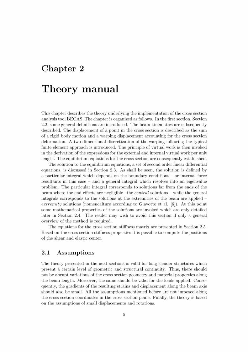
Figure 2.1: Cross section coordinate system.
2.2 Equilibrium equations
The derivation of the equilibrium equations for the beam cross section are presentedin this section.
2.2.1 Basic definitions
The reference coordinate system for a generic cross section with area A is presentedin Figure 2.1. The displacement of a point in the section s = [sx sy sz]
T is definedwith respect to the cross section coordinate system x, y, z . The strain and stress, ǫand σ, are given as
ǫT = [ǫxx ǫyy 2ǫxy 2ǫxz 2ǫyz ǫzz]
σT = [σxx σyy σxy σxz σyz σzz]
The stress and strain relate through Hooke’s law
σ = Qǫ (2.1)
where Q is the typical material constitutive matrix. It is assumed that the materialis linear elastic, otherwise there are no restrictions regarding the level of anisotropy(see Section 3.2). The ordering of the entries in ǫ and σ is such that the tractionsor the components of stress acting on the cross section face, can be easily isolatedin
pT = [σxz σyz σzz]
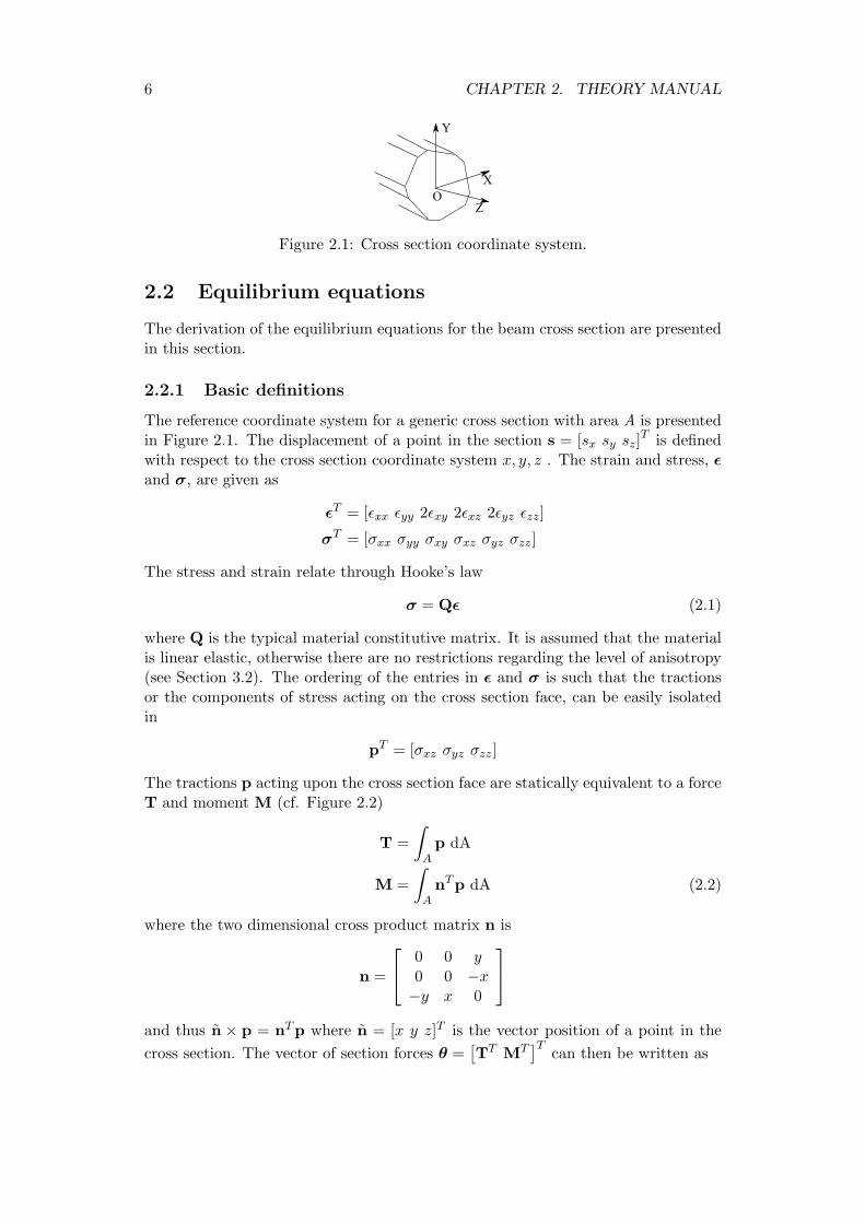
The tractions p acting upon the cross section face are statically equivalent to a forceT and moment M (cf. Figure 2.2)
T =
∫
Ap dA
M =
∫
AnTp dA (2.2)
where the two dimensional cross product matrix n is
n =
0 0 y0 0 −x−y x 0
and thus n × p = nTp where n = [x y z]T is the vector position of a point in the
cross section. The vector of section forces θ =[TT MT
]Tcan then be written as
2.2. EQUILIBRIUM EQUATIONS 7
Figure 2.2: Cross section resultant forces for a slice dx of the beam.
Figure 2.3: Schematic description of the different contributions for the deformationof the cross section.
θ =
∫
AZTp dA (2.3)
where the matrix Z =[I3|n
T], and Ii is the i th order identity matrix,
Z =
1 0 0 0 0 −y0 1 0 0 0 x0 0 1 y −x 0
2.2.2 Kinematics
The displacement s = [sx, sy, sz]T at a point of the cross section is defined as
s = v+ g
where v = [vx, vy, vz]T is the vector of displacements associated with the rigid body
translation and rotation of the cross section. The vector g = [gx, gy, gz]T is the
vector of warping displacements associated with the cross section deformation (seeFigure 2.3). Assuming small displacements and rotations, the rigid displacements vcan be obtained as
v = Zr
a linear combination of the the components of r =[χT ϕT
]T. The components of
χ(z) = [χx, χy, χz]T represent the translations of the cross section reference point,
while ϕ(z) = [ϕx, ϕy, ϕz]T are the cross section rotations. The total displacement
can be rewritten as
s = Zr+ g (2.4)
8 CHAPTER 2. THEORY MANUAL
2.2.3 Strain-displacement relation
The strain-displacement relation can be written as
ǫ = Bs+ S∂s
∂z(2.5)
where B and S are defined next. The strain displacement relation can then be castas
ǫxxǫyy2ǫxy2ǫxz2ǫyzǫzz
=
∂/∂x 0 00 ∂/∂y 0
∂/∂y ∂/∂x 00 0 ∂/∂x0 0 ∂/∂y0 0 0
︸ ︷︷ ︸
B
sxsysz
+
0 0 00 0 00 0 01 0 00 1 00 0 1
︸ ︷︷ ︸
S
∂sx/∂z∂sy/∂z∂sz/∂z
(2.6)
Note that this the common linear three dimensional strain-displacement relationwhere the terms ∂/∂z have been set appart. Inserting (2.4) into (2.5) yields
ǫ = BZr+ SZ∂r
∂z+Bg+ S
∂g
∂z(2.7)
It can be shown that
BZ = SZTr
where
Tr =
0 0 0 0 −1 00 0 0 1 0 00 0 0 0 0 00 0 0 0 0 00 0 0 0 0 00 0 0 0 0 0
Utilizing the relation above, Equation (2.7) can be written as
ǫ = SZ
(
Trr+∂r
∂z
)
+Bg+ S∂g
∂z
It is possible at this point to define the strain parameters
ψ = Trr+∂r
∂z(2.8)
and thus rewrite the strain displacement relation in its final form
ǫ = SZψ +Bg+ S∂g
∂z(2.9)
The section strain parameters ψ = [τx, τy, τz, κx, κy, κz]T are representative of
the strain due to the rigid displacement of two adjacent cross sections that remainundeformed. The components τx = ∂χx
∂z − ϕy and τy =∂χy
∂z + ϕx represent shearstrains of the cross section in the x and y directions, respectively. The component
τz = ∂χx
∂z is the axial elongation. Furthermore, κx = ∂ϕx∂z and κy =
∂ϕy
∂z are the
curvatures around x and y, respectively, and κz =∂ϕz∂z is the torsion term.
2.2. EQUILIBRIUM EQUATIONS 9
Finite element discretization
The warping displacements g are discretized as
g(x, y, z) = Ni(x, y)u(xi, yi, z) (2.10)
where N are the typical finite element shape functions and u the nodal warpingdisplacements. Note that the latter depend on the position along the beam axisalthough the shape functions are only defined in the plane of the section. Thedisplacement of a point in the cross section is then given as
s = Zr+Nu (2.11)
and finally introducing (2.10) in (2.9) yields
ǫ = SZψ +BNu+ SN∂u
∂z(2.12)
2.2.4 Virtual work principle
The total virtual work per unit length W is given as
W = We +Wi
The first variation of the total virtual work per unit length can be written as
δ∂W
∂z= δ
∂We
∂z+ δ
∂Wi
∂z(2.13)
where Wi is the work done by the internal elastic forces, and We the work done bythe external forces acting on the cross section.
External virtual work
Assuming that the surface and the body forces are zero, the axial derivative of thework produced by the section stresses is the only contribution to the external workWe. Thus(cf. Figure 2.2)
δ∂We
∂z=
∫
A
∂(δsTp
)
∂zdA
The external virtual work expression can be obtained by replacing the displacements as defined in (2.4) into the equation above
δ∂We
∂z=
∫
A
∂(δvTp
)
∂zdA +
∫
A
(δgTp
)
∂zdA
= δ∂rT
∂z
∫
AZTp dA + δrT
∫
AZT ∂p
∂zdA
︸ ︷︷ ︸
Work from rigid displacement
+ δ∂uT
∂z
∫
ANTp dA + δuT
∫
ANT ∂p
T
∂zdA
︸ ︷︷ ︸
Work from warping displacements
10 CHAPTER 2. THEORY MANUAL
Using Equation (2.3) it is possible to further simplify the previous equation
δ∂We
∂z= δ
∂rT
∂zθ + δrT
∂θ
∂z
+ δ∂uT
∂z
∫
ANTp dA + δuT
∫
ANT ∂p
T
∂zdA
Note that it is possible to introduce the strain parameters in the following manner
δ∂rT
∂zθ + δrT
∂θ
∂z=δ
∂rT
∂zθ + δrT
∂θ
∂z+ δrTTt
rθ − δrTTTr θ
=δrT∂θ
∂z− δrTTT
r θ + δ
(
rTTtr +
∂rT
∂z
)
︸ ︷︷ ︸
ψT
θ
=δrT∂θ
∂z− δrTTt
rθ + δψTθ
The expression for the external virtual work is then given as
δ∂We
∂z= δrT
∂θ
∂z− δrTTT
r θ + δψTθ
+ δ∂uT
∂z
∫
ANTp dA + δuT
∫
ANT ∂p
T
∂zdA
which in matrix form read as
δ∂We
∂z=
δ ∂uT
∂zδuδψ
T
P∂P∂zθ
+ δrT(∂θ
∂z−TT
r θ
)
(2.14)
where
P =
∫
ANTp dA
∂P
∂z=
∫
ANT ∂p
T
∂zdA
The vector P can be seen as the nodal stresses in the cross section finite elementdiscretization as it represents the discretized stresses acting on the cross section face.
Internal virtual work
The internal work or the work done by the elastic strain energy per unit length canbe written as
δ∂Wi
∂z=
∫
AδǫTσ dA (2.15)
Observing the stress-strain relation in Equation (2.1), the internal work expressionin (2.15) can be restated as
δ∂Wi
∂z=
∫
AδǫTQǫ dA
2.2. EQUILIBRIUM EQUATIONS 11
Inserting the expression for the strain-displacement relation in (2.12) in the equationabove yields
δ∂Wi
∂z=
∫
A
(
δψTZTST + δuTNTBT + δ∂uT
∂zNTST
)
Q
(
SZψ +BNu+ SN∂u
∂z
)
dA
=
∫
AδψTZTSTQSZψ dA
+
∫
AδψTZTSTQBNu dA
+
∫
AδψTZTSTQSN
∂u
∂zdA
+
∫
AδuTNTBTQSZψ dA
+
∫
AδuTNTBTQBNu dA
+
∫
AδuTNTBTQSN
∂u
∂zdA
+
∫
Aδ∂uT
∂zNTSTQSZψ dA
+
∫
Aδ∂uT
∂zNTSTQBNu dA
+
∫
Aδ∂uT
∂zNTSTQSN
∂u
∂zdA
where the following matrices can be identified
A =
∫
AZTSTQSZ dA
R =
∫
ANTBTQSZ dA
E =
∫
ANTBTQBN dA (2.16)
C =
∫
ANTSTQBN dA
L =
∫
ANTSTQSZ dA
M =
∫
ANTSTQSN dA
Hence, rearranging the state variables it is possible to write the internal virtual workin matrix form as
δ∂Wi
∂z=
δ ∂u∂zδuδψ
T
M C L
CT E R
LT RT A
∂u∂zuψ
(2.17)
12 CHAPTER 2. THEORY MANUAL
Total virtual work
According to Equation (2.13) the total virtual work per unit length can be writtenas
δ∂W
∂z= δ
∂We
∂z− δ
∂Wi
∂z=
∫
A
∂(δsTp
)
∂zdA−
∫
AδǫTσ dA (2.18)
For a general virtual displacement δs and virtual strain δǫ, a necessary and sufficientequilibrium condition is
δ∂W
∂z= 0
Thus, inserting Equation (2.14) and (2.17) into (2.18) the following relation is ob-tained
δ ∂u∂zδuδψ
T
M C L
CT E R
LT RT A
∂u∂zuψ
︸ ︷︷ ︸
Internal virtual work of the beam slice
=
=
δ ∂u∂zδuδψ
T
P∂P∂zθ
︸ ︷︷ ︸
External virtual work of the beam slice
+ δrT(∂θ
∂z−TT
r θ
)
︸ ︷︷ ︸
Equilibrium of the beam slice
The previous equation must be true for any admissible virtual displacement δψ,δu, δ ∂uT
∂z and δr, thus leading to the following set of equations
M∂u
∂z+CTu+ Lψ = P
C∂u
∂z+Eu+Rψ =
∂P
∂z
LT ∂u
∂z+RTu+Aψ = θ
∂θ
∂z= TT
r θ
It is possible to further simplify the former by differentiating the first equation withrespect to z
M∂2u
∂z2+CT ∂u
∂z+ L
∂ψ
∂z=
∂P
∂z
C∂u
∂z+Eu+Rψ =
∂P
∂z
LT ∂u
∂z+RTu+Aψ = θ
∂θ
∂z= TT
r θ
2.3. SOLUTIONS TO EQUILIBRIUM EQUATIONS 13
and obtain the equilibrium equations for the cross section
M∂2u
∂z2+(C−CT
) ∂u
∂z+ L
∂ψ
∂z−Eu−Rψ = 0
LT ∂u
∂z+RTu+Aψ = θ
∂θ
∂z= TT
r θ
(2.19)
This concludes the derivation of the equilibrium equations of the cross section.
2.3 Solutions to equilibrium equations
The set of equations in (2.19) admits two types of solutions – a particular integralwhich depends on the boundary conditions, or the internal force resultants θ inthis case, and a homogeneous integral which corresponds to the eigensolutions whenθ = 0. The homogeneous and particular solutions will be henceforth referred to asthe extremity and the central solutions (cf. Giavotto et al. [6]), respectively. Amore detailed discussion on this topic is presented in Section 2.4.
2.3.1 Extremity solutions
The extremitiy solutions owe their name to the fact that they correspond to thesolutions at the extremities of the beam where the loads are applied. These are theself-balanced, θ = 0, eigensolutions of (2.19), that is, the solutions to the followingset
M∂2u
∂z2+(C−CT
) ∂u
∂z+ L
∂ψ
∂z−Eu−Rψ = 0
LT ∂u
∂z+RTu+Aψ = 0
or in matrix form[M 00 0
] [ ∂2u∂z2∂2ψ∂z2
]
+
[ (C−CT
)L
−LT 0
] [ ∂u∂z∂ψ∂z
]
−
[E R
RT A
] [uψ
]
=
[00
]
(2.20)
Assuming solutions of the type
u = ueλz
ψ = ψeλz
and introducing the previous equation in (2.20) yields(
λ2
[M 00 0
]
+ λ
[ (C−CT
)L
−LT 0
]
−
[E R
RT A
])[u
ψ
]
= 0
The solution to (2.20) can be stated in terms of a linear combination of the solutionsto the eigenvalue problem
λ2
[M 00 0
]
+ λ
[ (C−CT
)L
−LT 0
]
−
[E R
RT A
]
= 0
14 CHAPTER 2. THEORY MANUAL
where λ are the eigenvalues and u and ψ the corresponding eigenvectors. The eigen-vectors represent the extremity modes and the corresponding eigenvalues define adiffusion length. The lowest eigenvalues are the most interesting as they propagatefarther into the beam. Choosing the eigenvectors corresponding to the lowest eigen-values it should be possible to study the effect of the loads at the extremities of thebeam. Nonetheless, the solution to this eigenvalue problem may be cumbersome asthe size of the matrices becomes larger.
2.3.2 Central solutions
The central solution refer to the solutions obtained at the central part of the beamcorresponding to non-zero stress resultants (θ 6= 0). For convenience, let us rewritethe equilibrium equations in (2.19) so that all the terms with derivatives of the sameorder are grouped
{
Eu+Rψ =(C−CT
)∂u∂z + L∂ψ
∂z +M∂2u∂z2
RTu+Aψ = −LT ∂u∂z + θ
(2.21)
At this point the reader may opt to read Section 2.4 first to get an insight into themathematical properties of the central solutions. Otherwise the necessary results toretain are that the central solutions uc and ψc are linear combinations of polynomialfunctions in z with n being the highest degree of such polynomials (see Equation(2.32) in Section 2.4.2). Thus
∂nuc
∂zn= 0 and
∂nψc
∂zn= 0
Furthermore, from the equilibrium equations for a rigid cross section (see Equation(2.28) in Section 2.4.1) the following must hold
∂2θ
∂z2= 0 (2.22)
and, recall from the equilibrium equations in (2.19) that
∂θ
∂z= TT
r θ (2.23)
We shall now utilize each of the results above to find an expression for the centralsolutions based on the set (2.21).
Let us consider the following sets which are obtained from the evaluation of thenth order derivative of set (2.21)
(0)
Eu+Rψ =(C−CT
)∂u∂z + L∂ψ
∂z +M∂2u
∂z2︸︷︷︸
=0
RTu+Aψ = −LT ∂u∂z + θ
↑ ∂u/∂z 6= 0 and ∂ψ/∂z 6= 0
(1)
E∂u∂z +R∂ψ
∂z =(C−CT
) ∂2u
∂z2︸︷︷︸
=0
+L∂2ψ
∂z2︸︷︷︸
=0
+M∂3u
∂z3︸︷︷︸
=0
RT ∂u∂z +A∂ψ
∂z = −LT ∂2u
∂z2︸︷︷︸
=0
+∂θ
∂z︸︷︷︸
6=0 from (2.23)
2.3. SOLUTIONS TO EQUILIBRIUM EQUATIONS 15
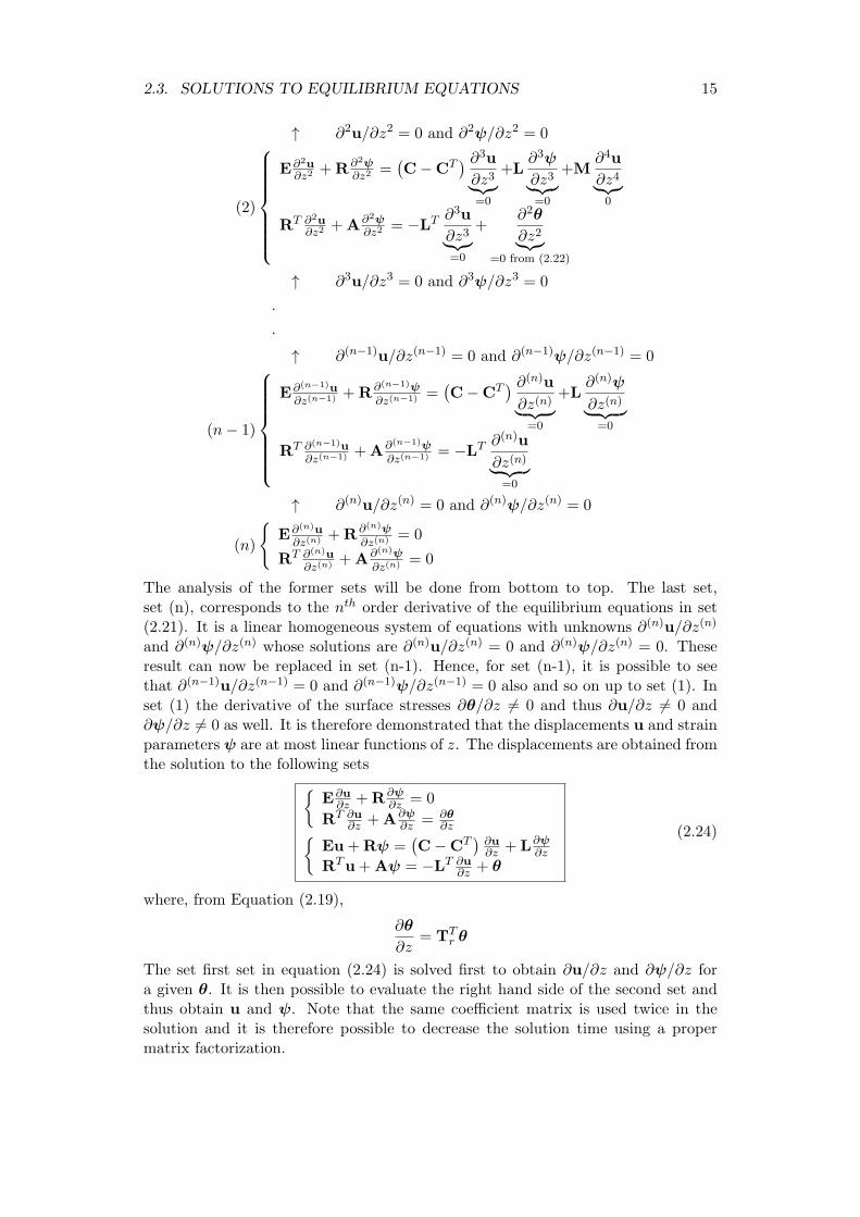
↑ ∂2u/∂z2 = 0 and ∂2ψ/∂z2 = 0
(2)
E∂2u∂z2
+R∂2ψ∂z2
=(C−CT
) ∂3u
∂z3︸︷︷︸
=0
+L∂3ψ
∂z3︸︷︷︸
=0
+M∂4u
∂z4︸︷︷︸
0
RT ∂2u∂z2
+A∂2ψ∂z2
= −LT ∂3u
∂z3︸︷︷︸
=0
+∂2θ
∂z2︸︷︷︸
=0 from (2.22)
↑ ∂3u/∂z3 = 0 and ∂3ψ/∂z3 = 0
.
.
↑ ∂(n−1)u/∂z(n−1) = 0 and ∂(n−1)ψ/∂z(n−1) = 0
(n− 1)
E∂(n−1)u
∂z(n−1) +R∂(n−1)ψ
∂z(n−1) =(C−CT
) ∂(n)u
∂z(n)︸ ︷︷ ︸
=0
+L∂(n)ψ
∂z(n)︸ ︷︷ ︸
=0
RT ∂(n−1)u
∂z(n−1) +A∂(n−1)ψ
∂z(n−1) = −LT ∂(n)u
∂z(n)︸ ︷︷ ︸
=0
↑ ∂(n)u/∂z(n) = 0 and ∂(n)ψ/∂z(n) = 0
(n)
{
E∂(n)u
∂z(n) +R∂(n)ψ
∂z(n) = 0
RT ∂(n)u
∂z(n) +A∂(n)ψ
∂z(n) = 0
The analysis of the former sets will be done from bottom to top. The last set,set (n), corresponds to the nth order derivative of the equilibrium equations in set(2.21). It is a linear homogeneous system of equations with unknowns ∂(n)u/∂z(n)
and ∂(n)ψ/∂z(n) whose solutions are ∂(n)u/∂z(n) = 0 and ∂(n)ψ/∂z(n) = 0. Theseresult can now be replaced in set (n-1). Hence, for set (n-1), it is possible to seethat ∂(n−1)u/∂z(n−1) = 0 and ∂(n−1)ψ/∂z(n−1) = 0 also and so on up to set (1). Inset (1) the derivative of the surface stresses ∂θ/∂z 6= 0 and thus ∂u/∂z 6= 0 and∂ψ/∂z 6= 0 as well. It is therefore demonstrated that the displacements u and strainparameters ψ are at most linear functions of z. The displacements are obtained fromthe solution to the following sets
{E∂u
∂z +R∂ψ∂z = 0
RT ∂u∂z +A∂ψ
∂z = ∂θ∂z
{Eu+Rψ =
(C−CT
)∂u∂z + L∂ψ
∂z
RTu+Aψ = −LT ∂u∂z + θ
(2.24)
where, from Equation (2.19),
∂θ
∂z= TT
r θ
The set first set in equation (2.24) is solved first to obtain ∂u/∂z and ∂ψ/∂z fora given θ. It is then possible to evaluate the right hand side of the second set andthus obtain u and ψ. Note that the same coefficient matrix is used twice in thesolution and it is therefore possible to decrease the solution time using a propermatrix factorization.
16 CHAPTER 2. THEORY MANUAL
2.3.3 Constraint equations
The displacement formulation as described in (2.11) is six times redundant. Eachof the redundancies corresponds to a description of each of the rigid body motionsand translations by the warping displacements u. It is therefore necessary to ensurethat the warping displacement u is uncoupled from the rigid displacements r. Thefollowing set of constraints are therefore incorporated into the solution of the sets(2.24)
nn∑
n=1
ux,n = 0,
nn∑
n=1
uy,n = 0,
nn∑
n=1
uz,n = 0,
nn∑
n=1
−znuy,n + ynuz,n = 0,
nn∑
n=1
znux,n − xnuz,n = 0,
nn∑
n=1
−ynux,n + xnuy,n = 0.
where nn is the number of nodes in the cross section finite element mesh, and(xn, yn, zn) and (ux,n, uy,n, uz,n) are the position and displacement of node n, respec-tively. The constraints are imposed on both the displacements u and correspondingderivatives ∂u/∂z and can be written in matrix form as
[DT 0
0 DT
] [u∂u∂z
]
=
[00
]
, where D =
[I3 ... I3n1 ... nnn
]T
where I3 is the 3 × 3 identity matrix, and nn is obtained from replacing the nodalcoordinates (xn, yn, zn) of node n in (2.2.1).
2.4 On the properties of the solutions
Some results used earlier in this manuscript to justify some of the steps in the deriva-tion of the cross section stiffness matrix of beams are described in this section. Inparticular, (2.28) and (2.32) are an important result in establishing the equilibriumequations for the central solutions in Section 2.3.2. The reader may skip this sectionaltogether if only a general overview of the method is necessary.
The section is divided in two parts. In the first part it is assumed that onlythe rigid body translations and rotations contribute to the displacement vector ofa point in the cross section, i.e., the cross section deformation is not accounted for.The equilibrium equations are derived and it is possible to show that the force andmoment resultants θ vary linearly with respect to z or along the beam length.
In the second part the displacement of a point in the cross section is obtainedthrough a finite element discretization of the warping displacements. The equilib-rium equations are derived once again. The result is a second order homogeneouslinear differential equation. The different types of solutions are identified accordingto Saint Venant’s principle. The solutions for which the eigenvalues are differentfrom zero will decay as z either increases or decreases. These are self-balanced(θ = 0) solutions corresponding to the modes at the extremities of the beam wherethe loads are applied – the extremity solutions. On the other hand, the solutionsfor which the eigenvalues are zero will not present any decay and, most importantly,it is possible to show that these will be polynomials in z. These correspond to non-zero stress resultants and account for the displacements at a section of the beam
2.4. ON THE PROPERTIES OF THE SOLUTIONS 17
sufficiently far from the extremities so that the influence of the external forces inthe stress field is negligible – the so-called central solutions.
2.4.1 Rigid motions
In this section we look only at the displacements v which do not strain the section,that is, we do not include the warping displacements. Thus
s = v = Zr = χ+ nϕ =
χx − yϕz
χy + xϕz
χz + yϕx − xϕy
(2.25)
recalling that χ = χ(z) and ϕ = ϕ(z) correspond to the translation of the crosssection reference point and rotations, respectively. The three dimensional straincomponents in this case are given by
ǫxx =1
2(∂vxx
+∂vxx
) = 0
ǫyy =1
2(∂vyy
+∂vyy
) = 0
2ǫxy =1
2(∂vyx
+∂vxy
) = 0
2ǫxz = (∂vzx
+∂vxz
) = −ϕy +∂χx
∂z− y
∂ϕz
∂z
2ǫyz = (∂vyz
+∂vzy
) =∂χy
∂z+ x
∂ϕz
∂z+ ϕx
ǫzz =1
2(∂vzz
+∂vzz
) =∂χz
∂z+ y
∂ϕx
∂z− x
∂ϕy
∂z
In matrix form the previous equations can be reduced to
p = tϕ+∂χ
∂z+ n
∂ϕ
∂z
where
t =
0 −1 01 0 00 0 0
It is convenient at this point to introduce the vector of strain parameters ψ =[τx, τy, τz, κx, κy, κz]
T defined in (2.8) and restated here as
ψ =
[ ∂χ∂z + tϕ
∂ϕ∂z
]
The three dimensional strain are hence
ǫ = SZψ (2.26)
Recalling the expression for the total work has been defined as
δ∂W
∂z=
∫
A
∂(pT δv
)
∂zdA−
∫
AσT δǫ dA = 0 (2.27)
18 CHAPTER 2. THEORY MANUAL
where the displacement s in (2.18) has been simply replaced here by v. Replacing(2.25) and (2.26) in (2.27) yields
δ∂W
∂z=
∫
A
∂(pT δχ+ pTnδϕ
)
∂zdA−
∫
AσTSZδψ dA
=
∫
A
∂pT δχ
∂zdA +
∫
A
pTnδϕ
∂zdA−
∫
AσTSZδψ dA
=
∫
A
∂pT
∂zδχ dA +
∫
ApT ∂δχ
∂zdA +
∫
A
pT
∂znδϕ dA +
∫
ApTn
δϕ
∂zdA
−
∫
AσTSZδψ dA
=
∫
A
∂pT
∂zdA
︸ ︷︷ ︸
∂T/∂z
δχ+
∫
ApT dA
︸ ︷︷ ︸
T
∂δχ
∂z+
∫
A
pT
∂zn dA
︸ ︷︷ ︸
∂M/∂z
δϕ+
∫
ApTn dA
︸ ︷︷ ︸
M
δϕ
∂z
−
∫
AσTSZδψ dA
=∂TT
∂zδχ+TT ∂δχ
∂z+
∂MT
∂zδϕ+MT δϕ
∂z−
∫
AσTSZδψ dA
Noting that
θTψ = TT ∂χ
∂z−TT tϕ+MT ∂ϕ
∂z
it is possible to further simplify in the following manner
δ∂W
∂z=∂TT
∂zδχ+TT ∂δχ
∂z+
∂MT
∂zδϕ+MT δϕ
∂z−
∫
AσTSZδψ dA
=∂TT
∂zδχ+TT ∂δχ
∂z+
∂MT
∂zδϕ+MT δϕ
∂z−TT tδϕ+TT tδϕ︸ ︷︷ ︸
for convenience
−
∫
AσTSZδψ dA
=∂TT
∂zδχ+
∂MT
∂zδϕ+TT tδϕ+TT ∂δχ
∂z+MT δϕ
∂z−TT tδϕ
︸ ︷︷ ︸
θT δψ
−
∫
AσTSZδψ dA
=∂TT
∂zδχ+
(∂MT
∂z+TT t
)
δϕ+
(
θT −
∫
AσTSZ dA
)
δψ
and isolate each of the variation terms in the equation. Thus, for the arbitraryvariation of δψ we get
θ =
∫
AZSσ dA
where p = Sσ. The equation above is the definition of the resultant forces actingon the cross section as stated in (2.2). Subsequently, for the arbitrary variation ofδϕ and δχ we obtain, respectively
∂MT
∂z= −TT t ,
∂TT
∂z= 0
2.4. ON THE PROPERTIES OF THE SOLUTIONS 19
The two expressions above are the equilibrium equations or the one dimensionalbeam equations when only the cross section rigid displacements are considered.These equations are typically obtained from simple statitcs and so this result showsthe consistency between the one and three dimensional approaches. Furthermore,based on the results above it is possible to conclude that
∂2MT
∂z2= 0
and so
∂2θ
∂z2= 0 (2.28)
The equation above states that the resulting forces acting on the section vary linearlyalong the beam.
2.4.2 Warping displacements
In this section we assume that
s = g
The displacement of a point in the cross section is given here as a function of the crosssection deformation only. Note however that this definition of the displacementsentails also the representation of the rigid translation χ and rotation ϕ. This is infact the underlying motivation for the use of constraint equations as described inSection 2.3.3 to uncouple the rigid body motions and cross section deformation.
The stress-strain relation in this case is given as
ǫ = Bg+ S∂g
∂z
and the expression for the variation of the total energy is
δ∂W
∂z=
∫
A
∂(pT δs
)
∂zdA−
∫
AσT δǫ dA
Recalling the generalized Hooke’s law σ = Qǫ and noting that p = Sσ,theexpression for the total virtual work of the beam cross section considering only the
20 CHAPTER 2. THEORY MANUAL
warping displacements is given by
δ∂W
∂z=
∫
A
∂(σTSδg
)
∂zdA−
∫
AσT
(
Bδg+ S∂δg
∂z
)
dA
=
∫
A
∂σT
∂zSδg dA +
∫
AσTS
∂δg
∂zdA
−
∫
AσTBδg dA−
∫
AσTS
∂δg
∂zdA
=
∫
A
∂σT
∂zSδg dA−
∫
AσTBδg dA
=
∫
A
∂ǫT
∂zQSδg dA−
∫
AǫTQBδg dA
=
∫
A
∂gT
∂zBTQSδg dA +
∫
A
∂2gT
∂z2STQSδg dA
−
∫
AgTBTQBδg dA−
∫
A
∂gT
∂zSTQBδg dA
(2.29)
Expanding g using the typical finite element approach (cf. Equation (2.10))
g(x, y, z) = Ni(x, y)u(xi, yi, z) (2.30)
and replacing (2.30) in (2.29) yields
δ∂W
∂z=
∫
A
∂uT
∂zNTBTQSNδu dA +
∫
A
∂2uT
∂z2NTSTQSNδu dA
−
∫
AuTNTBTQBNδu dA−
∫
A
∂uT
∂zNTSTQBNδu dA
From the equation above it is possible then to identify the matrices
M =
∫
ANTSTQSN dA
C =
∫
ANTBTQSN dA
E =
∫
ANTBTQBN dA
where M and E are symmetrical while H = C−CT is skew-symmetrical. Rewritingthe total virtual work expression
δ∂W
∂z=δu
(
M∂2u
∂z2−H
∂u
∂z−Eu
)
The following must hold for an arbitrary variation of δu
M∂2u
∂z2−H
∂u
∂z−Eu = 0 (2.31)
This concludes the derivation of the equilibrium equations for the cross sectionconsidering only the warping displacements. The aim now is not to solve the equation
2.4. ON THE PROPERTIES OF THE SOLUTIONS 21
above but rather discuss the properties of the solutions for this second order linearhomogeneous differential equation.
The general solution is sought as a linear combination of
u(z) = heλz
Inserting the above into (2.31) yields
(λ2M− λH−E
)h = 0
where h are the eigenvectors associated with the eigenvalues λ resulting from thesolution to
λ2M− λH−E = 0
According to physical considerations and Saint-Venant’s principle, we expect tohave a self-balanced (θ = 0) solution associated with the exponentially decayingmodes (λ 6= 0) – extremity solutions – and a solution presenting no decay (λ = 0)for which the stress resultants are non-zero (θ 6= 0) – central solutions (see [6]).
Owing to the structure of matrices M, E and H (and mostly due to the fact thatH is skew-symmetric), for the extremity solutions the eigenvalues will be complexand come in pairs. That is, to each eigenvalue λj = a+ ib corresponds a second λj =a − ib. The solution corresponding to the first eigenvalue decays while z increases(moving away from the first end of the beam), wheras the solution associated withthe second eigenvalue in the pair is identical but decays as z decreases (moving awayfrom the second end of the beam). This solutions can be used to study end effectsand determining the diffusion length or the distance at which the effects from theexternal loads become negligble (e.g., see Horgan [18] and Choi and Horgan [19] fora discussion on the diffusion length in anisotropic elasticity).
The central solutions for which θ 6= 0, on the other hand, do not have anyexponential decay as they correspond to eigenvalues λj = 0 with multiplicity pj .These are the solutions at the central part of the beam sufficiently away from theextremities so that the effect from the external loads is negligible on the stress field.The solutions for problems where λj = 0 and its multiplicity pj ≥ 2, are given as(see [21] for a comprehensive presentation of this topic)1
u1j(z) = h11eλjz
u2j(z) = h21eλjz + h22ze
λz
.
.
upjj(z) = hpj1eλjz + hpj2ze
λjz + ...+ zpj−1hpjpjeλjz
where the corresponding solution in this case is
uj(z) =c1h11eλjz + c2 (h21 + zh22) e
λjz + ...
+ cpj(h21 + zh22 + ...+ zpj−1hpjpj
)eλjz
1The authors would like to express its gratitude to Assoc. Prof. Mads Peter Sı¿ 12rensen (DTU-
MAT) for all the help unravelling this step of the derivation.
22 CHAPTER 2. THEORY MANUAL
In our specific case where λj = 0 the solutions in this case are of the polynomialtype
uj(z) =c1h11 + c2 (h21 + zh22) + ...+ cp(h21 + zh22 + ...+ zpj−1hpjpj
)
A central solution uc will be any linear combination of the solutions uj for whichλj = 0. If n is the maximum of all pj then
∂nuc
∂zn= 0 (2.32)
Thus the central solutions are polynomial functions in z of at most degree n.
2.5 Cross section properties
We look first for the compliance matrix of a cross section of the beam. That is weare interested in finding an expression for the strain energy as function of the stressresultants and moments. These are in fact the central solutions derived above – aparticular solution depending on the applied section forces at a given cross sectionsubject to particular boundary conditions which guarantee that the effects of theextremity solutions are negligible. A procedure is presented in this section for thepractical determination of the cross section stiffness matrix based on the result ofthe central solutions. Finally expressions for the determination of the shear andelastic center are derived.
2.5.1 Cross section stiffness matrix
From Equation (2.24) it is important to note that the central solutions are linearand homogeneous2 functions of the force resultants. Thus it is possible to write
u = Xθ,∂u
∂z=
∂X
∂zθ
ψ = Yθ,∂ψ
∂z=
∂Y
∂zθ
(2.33)
Inserting the expressions above in (2.24) yields
{EX+RY =
(C−CT
)∂X∂z + L∂Y
∂z
RTX+AY = −LT ∂X∂z + I6
{E∂X
∂z +R∂Y∂z = 0
RT ∂X∂z +A∂Y
∂z = TTr
(2.34)
Note that the set of equations above can be obtained by replacing θ = I6 in (2.24).This corresponds to determining the central solutions for six different choices of thestress resultant θ in an orderly way, i.e., setting one of the entries to unity and theremaining to zero. In fact, each of the six columns of X, Y, ∂X
∂z and ∂Y∂z hold the
corresponding displacement solution for each of the different stress resultants.
2An homogeneous function is such that f(αx) = αf(x). In this specific case, one importantinference is that homogeneous functions do not have an independent term.
2.5. CROSS SECTION PROPERTIES 23
Restating the expression for the variation of the total energy obtained from thevirtual work principle
δ∂W
∂z=
∫
A
∂(pT δv
)
∂zdA−
∫
AσT δǫ dA = 0
The previous equation can be restated as
δθTFsθ =
∫
AσT δǫ dA
where Fs is the compliance matrix of the section. The strain is redefined by inserting(2.33) in (2.12)
ǫ = SZYθ +BNXθ + SN∂X
∂zθ
which then yields for the internal energy
δ∂Wi
∂z=
∫
Aδθ
(
YTZTST +XTNTBT +∂XT
∂zNTST
)
Q
(
SZY+BNX+ SN∂X
∂z
)
θ dA
The former can be stated in matrix form as
δ∂Wi
∂z=
δθX
δθ ∂X∂z
δθY
T
E C R
CT M L
RT LT A
Xθ∂X∂z θ
Yθ
The total virtual work expression becomes
δθTFsθ =
δθX
δθ ∂X∂z
δθY
T
E C R
CT M L
RT LT A
Xθ∂X∂z θ
Yθ
For any admissible virtual displacement δθX, δθ ∂X∂z and δθY it is possible to obtain
an expression for the cross section compliance matrix defined as
Fs =
X∂X∂zY
T
E C R
CT M L
RT LT A
X∂X∂zY
The corresponding stiffness matrix Ks can be computed as
Ks = F−1s (2.35)
This result can be used to generate beam finite element models for which the strainscan be exactly described by the six strain parameters in ψ. The material maybe anisotropic, inhomogeneously distributed, and the reference coordinate systemmay be arbitrarily located. The stiffness matrix Ks will correctly account for anygeometrical or material couplings.
24 CHAPTER 2. THEORY MANUAL
2.5.2 Shear center and elastic center positions
The expressions for the positions of the shear and elastic center are presented next.The shear center is defined as the point at which a load applied parallel to the
plane of the section will produce no torsion (i.e., κz = 0). Hence, assume that twotransverse forces, Tx and Ty are applied at a point (xs, ys) at a given cross section.The moments induced by the two forces are
Mx = −Ty(L− z) , My = Tx(L− z) , Mz = −Txys + Tyxs (2.36)
The aim is to find the position (xs, ys) for which the curvature associated withthe twist κz = 0. Thus, taking into account the cross section constitutive relationψ = Fsθ, the following holds
κz = Fs,61Tx + Fs,62Ty + Fs,64Mx + Fs,65My + Fs,66Mz = 0
Inserting (2.36) into the previous equation yields
[Fs,61 + Fs,62(L− z)− Fs,66ys]Tx + [Fs,62 − Fs,64(L− z) + Fs,66xs]Ty = 0
Since the above has to be valid for any Tx and Ty,
xs = −Fs,62 + Fs,64(L− z)
Fs,66
ys =Fs,61 + Fs,65(L− z)
Fs,66
From the previous equation it can be seen that the shear center is not a property ofthe cross section. Instead, in the case where the entries Fs,64 and Fs,65 associatedwith the bending-twist coupling are not zero, the position of the shear center varieslinearly along the beam length .
The expressions for the position of the elastic center can be determined in thesame manner. The elastic center is defined as the point where a force applied normalto the cross section will produce no bending curvatures (i.e., κx = κy = 0). Thus,assume that a load Tz is applied at the point (xt, yt) in the cross section. Themoments induced by this force are
Mx = Tzyt , My = −Tzxt (2.37)
We look for the positions (xt, yt) for which κx = κy = 0. From the cross sectionconstitutive relation,
κx = Fs,43Tz + Fs,44Mx + Fs,45My = 0
κx = Fs,53Tz + Fs,54Mx + Fs,55My = 0
Since the previous must be valid for any force Tz, inserting (2.37) into the previousequation will result in the following set of linear equations
{Fs,43 + Fs,44yt − Fs,45xt = 0Fs,53 + Fs,54yt − Fs,55xt = 0
2.6. CROSS SECTION MASS MATRIX 25
and so
xt = −−Fs,44Fs,53 + Fs,45Fs,43
Fs,44Fs,55 − F 2s,45
yt = −Fs,43Fs,55 − Fs,45Fs,53
Fs,44Fs,55 − F 2s,45
which are the expressions for the position of the elastic center.
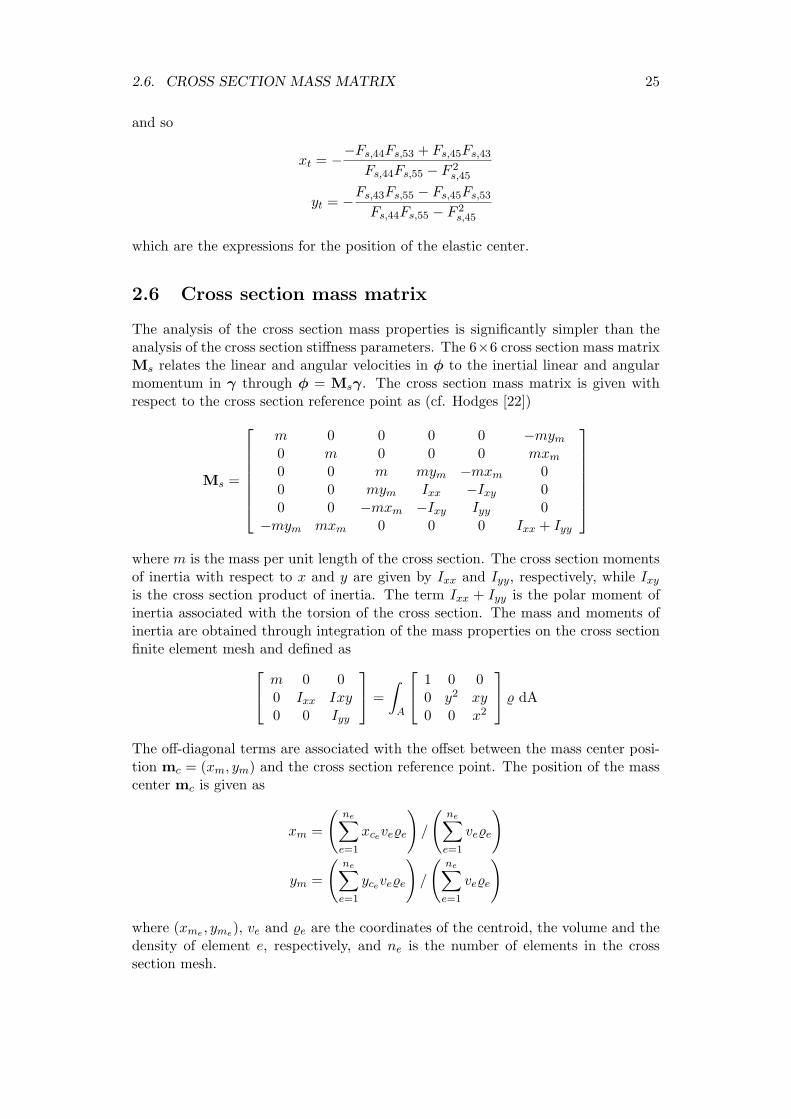
2.6 Cross section mass matrix
The analysis of the cross section mass properties is significantly simpler than theanalysis of the cross section stiffness parameters. The 6×6 cross section mass matrixMs relates the linear and angular velocities in φ to the inertial linear and angularmomentum in γ through φ = Msγ. The cross section mass matrix is given withrespect to the cross section reference point as (cf. Hodges [22])
Ms =
m 0 0 0 0 −mym0 m 0 0 0 mxm0 0 m mym −mxm 00 0 mym Ixx −Ixy 00 0 −mxm −Ixy Iyy 0
−mym mxm 0 0 0 Ixx + Iyy
where m is the mass per unit length of the cross section. The cross section momentsof inertia with respect to x and y are given by Ixx and Iyy, respectively, while Ixyis the cross section product of inertia. The term Ixx + Iyy is the polar moment ofinertia associated with the torsion of the cross section. The mass and moments ofinertia are obtained through integration of the mass properties on the cross sectionfinite element mesh and defined as
m 0 00 Ixx Ixy0 0 Iyy
=
∫
A
1 0 00 y2 xy0 0 x2
dA
The off-diagonal terms are associated with the offset between the mass center posi-tion mc = (xm, ym) and the cross section reference point. The position of the masscenter mc is given as
xm =
(ne∑
e=1
xcevee
)
/
(ne∑
e=1
vee
)
ym =
(ne∑
e=1
ycevee
)
/
(ne∑
e=1
vee
)
where (xme , yme), ve and e are the coordinates of the centroid, the volume and thedensity of element e, respectively, and ne is the number of elements in the crosssection mesh.
26 CHAPTER 2. THEORY MANUAL
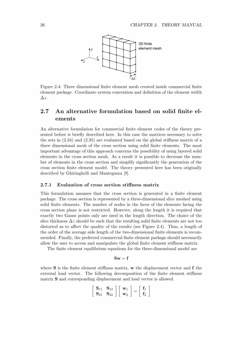
xz
y
Δz
3D finite
element mesh
Figure 2.4: Three dimensional finite element mesh created inside commercial finiteelement package. Coordinate system convention and definition of the element width∆z.
2.7 An alternative formulation based on solid finite el-
ements
An alternative formulation for commercial finite element codes of the theory pre-sented before is briefly described here. In this case the matrices necessary to solvethe sets in (2.34) and (2.35) are evaluated based on the global stiffness matrix of athree dimensional mesh of the cross section using solid finite elements. The mostimportant advantage of this approach concerns the possibility of using layered solidelements in the cross section mesh. As a result it is possible to decrease the num-ber of elements in the cross section and simplify significantly the generation of thecross section finite element model. The theory presented here has been originallydescribed by Ghiringhelli and Mantegazza [9].
2.7.1 Evaluation of cross section stiffness matrix
This formulation assumes that the cross section is generated in a finite elementpackage. The cross section is represented by a three-dimensional slice meshed usingsolid finite elements. The number of nodes in the faces of the elements facing thecross section plane is not restricted. However, along the length it is required thatexactly two Gauss points only are used in the length direction. The choice of theslice thickness ∆z should be such that the resulting solid finite elements are not toodistorted as to affect the quality of the results (see Figure 2.4). Thus, a length ofthe order of the average side length of the two-dimensional finite elements is recom-mended. Finally, the preferred commercial finite element package should necessarilyallow the user to access and manipulate the global finite element stiffness matrix.
The finite element equilibrium equations for the three-dimensional model are
Sw = f
where S is the finite element stiffness matrix, w the displacement vector and f theexternal load vector. The following decomposition of the finite element stiffnessmatrix S and corresponding displacement and load vector is allowed
[S11 S12
S21 S22
] [w1
w2
]
=
[f1f2
]
2.7. AN ALTERNATIVE FORMULATION BASEDON SOLID FINITE ELEMENTS27
where the index 1 and 2 refer to the contributions from the nodes at z = 0 andz = ∆z, respectively,. Based on the above submatrices Ghiringhelli and Mantegazza[9] have derived the expressions for the matrices necessary for the computation ofthe cross section stiffness matrix. Hence, after proper derivation the following aredefined
M = ((S11 + S22)− 2 (S12 + S21))∆z
6
C =1
2((S11 − S22)− (S12 − S21))
E = (S11 + S22 + S12 + S21)1
∆z
Note that deriving the original equations in Ghiringhelli and Mantegazza [9] yieldsthe 1/2 factor in matrixC. This factor is not present in the derviation by Ghiringhelliand Mantegazza [9]. The remaining matrices can be determined as
R = CZG, L = MZG, A = ZTGMZG
where ZG is defined as
ZG =
1 0 0 0 0 −y10 1 0 0 0 x10 0 1 y1 −x1 0
...1 0 0 0 0 −ynn
0 1 0 0 0 xnn
0 0 1 ynn −xnn 0
where nn is the number of nodes in the reference cross section face (i.e., half thenodes in the whole three dimensional model). Having defined all the matrices it ispossible now to solve the sets (2.34) while remembering to account for the matrixof constraint equations D presented in 2.3.3. Replacing the solutions of (2.34) into(2.35) it is straight forward to evaluate the cross section stiffness matrix Ks.
The formulation presented here has been implemented in the class of Matlabfunctions BECAS_3D.

28 CHAPTER 2. THEORY MANUAL
Chapter 3
Implementation manual
The theory presented in the previous sections up to the determination of the crosssection stiffness matrix and, shear and elastic centers, is implemented in the BEamCross section Analysis Software – BECAS. This section addresses the practical im-plementation of the theory. The MATLAB implementation of BECAS described inAppendix 5 is according to the expressions described in this section.
Two different approaches have been implemented. The first approach is basedon a two dimensional finite element mesh and is mostly attractive for readers whichwork on their own finite element code. The second approach is based on a threedimensional mesh of the cross section using eight node solid finite elements. Theapproach is described in detail in Ghiringhelli and Mantegazza [9] and only the mostimportant results are presented here. The approach is implemented in BECAS forillustrative purposes only.
Although these are standard procedures, the transformation of the materialconstitutive matrix is a topic where, in the authors’ opinion, there is often someambiguity concerning specific definitions for specific implementations. Hence, thefinal section of this chapter has been dedicated to the presentation of the mate-rial constitutive matrix for orthotropic materials and the corresponding necessarytransformations.
3.1 Two dimensional finite element analysis
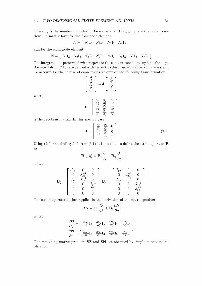
3.1.1 Q4 and Q8 elements
The first step in the evaluation of the cross section properties is the generation of atwo dimensional finite element mesh of the cross section. An example of a discretizedprofile section using Q4 elements is presented in Figure 3.1. The material properties,fiber plane orientation and fiber directions are defined at each element of the finiteelement mesh. Thus, a layer of a certain material is defined using a layer of elements.Having defined the cross section mesh and material properties, the subsequent stepconcerns the derivation of each of the matrices in Equation (2.16).
The implementation is based on four or eight node isoparametric elements. Thenode numbering and isoparametric coordinate system are presented in Figure 3.2.The shape functions employed in the derivation of the four node isoparametric finite
29
30 CHAPTER 3. IMPLEMENTATION MANUAL
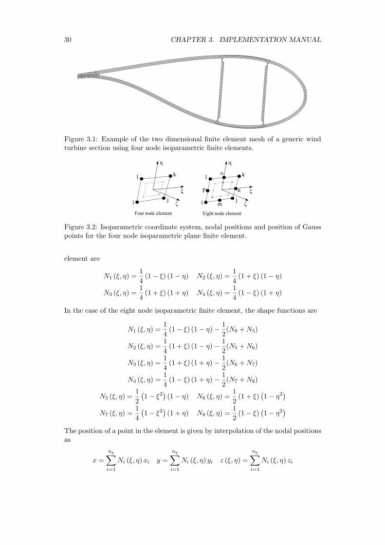
Figure 3.1: Example of the two dimensional finite element mesh of a generic windturbine section using four node isoparametric finite elements.
i j
kl
ξ
η
ζ
Four node element
i j
kl
ξ
η
ζ
Eight node element
m
n
o
p
Figure 3.2: Isoparametric coordinate system, nodal positions and position of Gausspoints for the four node isoparametric plane finite element.
element are
N1 (ξ, η) =1
4(1− ξ) (1− η) N2 (ξ, η) =
1
4(1 + ξ) (1− η)
N3 (ξ, η) =1
4(1 + ξ) (1 + η) N4 (ξ, η) =
1
4(1− ξ) (1 + η)
In the case of the eight node isoparametric finite element, the shape functions are
N1 (ξ, η) =1
4(1− ξ) (1− η)−
1
2(N8 +N5)
N2 (ξ, η) =1
4(1 + ξ) (1− η)−
1
2(N5 +N6)
N3 (ξ, η) =1
4(1 + ξ) (1 + η)−
1
2(N6 +N7)
N4 (ξ, η) =1
4(1− ξ) (1 + η)−
1
2(N7 +N8)
N5 (ξ, η) =1
2
(1− ξ2
)(1− η) N6 (ξ, η) =
1
2(1 + ξ)
(1− η2
)
N7 (ξ, η) =1
4
(1− ξ2
)(1 + η) N8 (ξ, η) =
1
2(1− ξ)
(1− η2
)
The position of a point in the element is given by interpolation of the nodal positionsas
x =
nq∑
i=1
Ni (ξ, η)xi y =
nq∑
i=1
Ni (ξ, η) yi z (ξ, η) =
nq∑
i=1
Ni (ξ, η) zi
3.1. TWO DIMENSIONAL FINITE ELEMENT ANALYSIS 31
where nq is the number of nodes in the element, and (xi, yi, zi) are the nodal posi-tions. In matrix form for the four node element
N =[N1I3 N2I3 N3I3 N4I3
]
and for the eight node element
N =[N1I3 N2I3 N3I3 N4I3 N5I3 N5I3 N7I3 N8I3
]
The integration is performed with respect to the element coordinate system althoughthe integrals in (2.16) are defined with respect to the cross section coordinate system.To account for the change of coordinates we employ the following transformation
∂∂ξ∂∂η∂∂ζ
= J
∂∂x∂∂y∂∂z
where
J =
∂x∂ξ
∂y∂ξ
∂z∂ξ
∂x∂η
∂y∂η
∂z∂η
∂x∂ζ
∂y∂ζ
∂z∂ζ
is the Jacobian matrix. In this specific case
J =
∂x∂ξ
∂y∂ξ 0
∂x∂η
∂y∂η 0
0 0 1
(3.1)
Using (2.6) and finding J−1 from (3.1) it is possible to define the strain operator Bas
B(ξ, η) = Bξ∂
∂ξ+Bη
∂
∂η
where
Bξ =
J−111 0 0
0 J−121 0
J−121 J−1
11 0
0 0 J−111
0 0 J−121
0 0 0
Bη =
J−112 0 0
0 J−122 0
J−122 J−1
12 0
0 0 J−112
0 0 J−122
0 0 0
The strain operator is then applied in the derivation of the matrix product
BN = Bξ∂N
∂ξ+Bη
∂N
∂η
where
∂N
∂ξ=[
∂N1∂ξ I3
∂N2∂ξ I3
∂N3∂ξ I3
∂N4∂ξ I3
]
∂N
∂η=[
∂N1∂η I3
∂N2∂η I3
∂N3∂η I3
∂N4∂η I3
]
The remaining matrix products SZ and SN are obtained by simple matrix multi-plication.
32 CHAPTER 3. IMPLEMENTATION MANUAL
3.1.2 Local and global finite element matrices
The integration is performed at the element level and hence the element matricesare evaluated as
Ae =
∫
AZTSTQSZ dxdy =
∫
AZTSTQSZ |J | dξ dη
Re =
∫
ANTBTQSZ dxdy =
∫
ANTBTQSZ |J | dξ dη
Ee =
∫
ANTBTQBN dxdy =
∫
ANTBTQBN |J | dξ dη
Ce =
∫
ANTBTQSN dxdy =
∫
ANTBTQSN |J | dξ dη
Le =
∫
ANTSTQSZ dxdy =
∫
ANTSTQSZ |J | dξ dη
Me =
∫
ANTSTQSN dxdy =
∫
ANTSTQSN |J | dξ dη
where the integration is performed using a four point Gauss quadrature (cf. Figure3.2). The global matrices are subsequently assembled following typical finite elementprocedures
A =
ne∑
i=1
Ae , R =
ne∑
i=1
Re , E =
ne∑
i=1
Ee
C =
ne∑
i=1
Ce , L =
ne∑
i=1
Le , M =
ne∑
i=1
Me
where ne is the number of finite elements in the cross section mesh.Having obtained each of the matrices it is possible to finally solve the cross
section equilibrium equations
E R D
RT A 0
DT 0 0
XYΛ2
=
(C−CT
)L
LT 00 0
[∂X∂z∂Y∂z
]
+
0I0
E R D
RT A 0
DT 0 0
∂X∂z∂Y∂zΛ1
=
0
TTr
0
where D is the matrix of contraint equations defined in 2.3.3, and Λ1 and Λ2 arethe corresponding Lagrange multipliers. The two sets above make use of the samecoefficient matrix and can be solved efficiently using a proper factorization (e.g.,LU factorization). The solutions are then obtained doing a forward and backwardsubstitution.
The cross section compliance matrix is then readily obtained by inserting thesolutions of the previous set into
Fs =
X∂X∂zY
T
E C R
CT M L
RT LT A
X∂X∂zY
3.2. MATERIAL CONSTITUTIVE MATRIX 33
A MATLAB implementation of BECAS according to the theory presented aboveis described in Chapter 5.
3.2 Material constitutive matrix
At each element of the cross section finite element mesh, the user of BECAS mustspecify
• Material properties
• Orientation of the laminate plane
• Orientation of the fibers laminate
Based on this input, the first step consists of assembling the material constitutivematrix in the material coordinate system based on a set of material properties.
3.2.1 Definition
In the case of orthotropic materials, the stress-strain relation or generalized Hookes’Law is stated as
σ22σ33σ23σ12σ13σ11
=
1E22
− ν23E22
0 0 0 − ν21E11
− ν23E22
1E33
0 0 0 − ν31E11
0 0 1G23
0 0 0
0 0 0 1G12
0 0
0 0 0 0 1G13
0
− ν2zE11
− ν13E11
0 0 0 1E11
−1
︸ ︷︷ ︸
Q
γ22γ33γ23γ12γ13γ11
where the material properties are given in the material coordinate system (see Figure3.3c) and defined as
• E11 the Young modulus of material the 1 direction.
• E22 the Young modulus of material the 2 direction.
• E33 the Young modulus of material the 3 direction.
• G12 the shear modulus in the 12 plane.
• G13 the shear modulus in the 13 plane.
• G23 the shear modulus in the 23 plane.
• ν12 the Poisson’s ratio in the 12 plane.
• ν13 the Poisson’s ratio in the 13 plane.
• ν23 the Poisson’s ratio in the 23 plane.
• the material density.
34 CHAPTER 3. IMPLEMENTATION MANUAL
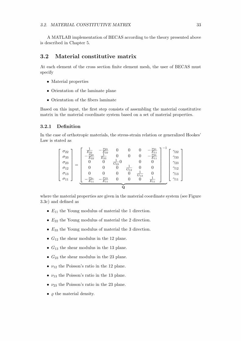
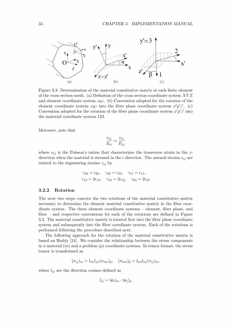
(a) (b)
x'
y'
z'1
2
3
β(c)
Figure 3.3: Determination of the material constitutive matrix at each finite elementof the cross section mesh. (a) Definition of the cross section coordinate system XY Zand element coordinate system xyz. (b) Convention adopted for the rotation of theelement coordinate system xyz into the fiber plane coordinate system x′y′z′. (c)Convention adopted for the rotation of the fiber plane coordinate system x′y′z′ intothe material coordinate system 123.
Moreover, note that
νijEii
=νjiEjj
where νij is the Poisson’s ration that characterizes the transverse strain in the j-direction when the material is stressed in the i direction. The natural strains ǫij arerelated to the engineering strains γij by
γ22 = ǫ22, γ33 = ǫ33, γ11 = ǫ11,
γ13 = 2ǫ13, γ12 = 2ǫ12, γ23 = 2ǫ23
3.2.2 Rotation
The next two steps concern the two rotations of the material constitutive matrixnecessary to determine the element material constitutive matrix in the fiber coor-dinate system. The three element coordinate systems – element, fiber plane, andfiber – and respective conventions for each of the rotations are defined in Figure3.3. The material constitutive matrix is rotated first into the fiber plane coordinatesystem and subsequently into the fiber coordinate system. Each of the rotations isperformed following the procedure described next.
The following approach for the rotation of the material constitutive matrix isbased on Reddy [24]. We consider the relationship between the stress componentsin a material (m) and a problem (p) coordinate systems. In tensor format, the stresstensor is transformed as
(σij)m = limljn(σmn)p, (σmn)p = lmilnj(σij)m,
where lij are the direction cosines defined as
lij = (ei)m · (ej)p
3.2. MATERIAL CONSTITUTIVE MATRIX 35
The vectors e are unit vectors associated with the axis at each of the coordinatesystems. The components of the stress in the material and problem coordinatesystems are
σm = [σxxm σyym σxym σxzm σyzm σzzm ]T
σp =[σxxp σyyp σxyp σxzp σyzp σzzp
]T
The 3× 3 arrays with the stress components are given by
σm =
σxxm σxym σxzmσyxm σyym σyzmσzxm σzym σzzm
, σp =
σxxp σxyp σxzpσyxp σyyp σyzpσzxp σzyp σzzp
where the (ˆ) refers to the array notation. Then the rotations in Equation 3.2.2 canbe expressed as
σm = LσpLT , σp = LT σmL
The vector of engineering strains in the material and problem coordinate systems is
γm = [γxxm γyym γzzm γyzm γxzm γxym ]T
γp =[γxxp γyyp γzzp γyzp γxzp γxyp
]T
The natural strain components may be defined in function of the engineering strainsas
ǫm =
γxxm12γxym
12γxzm
12γyxm γyym
12γyzm
12γzxm
12γzym γzzm
, ǫp =
γxxp12γxyp
12γxzp
12γyxp γyyp
12γyzp
12γzxp
12γzyp γzzp
where γ are the engineering strains. Since the strains are also second order tensors,the relations derived for the stresses are also valid for the strains
ǫm = LǫpLT , ǫp = LT ǫmL
Based on the expressions presented before it is possible to establish the equationsfor the transformation of the material constitutive matrix. The constitutive matrixin the problem coordinate system, Qp, is obtained by transformation of the materialconstitutive matrix in the material coordinate system, Qm. The following stepsshould be followed in the rotation of the material constitutive matrix:
1. The array ǫp is assembled based on the engineering strains γp remembering toobserve the 1/2 factor;
2. The strains are then rotated employing ǫm = LǫpLT ;
3. Having ǫm it is possible to assemble the vector of engineering strains γm
remembering to multiply by 2 the natural shear strain components;
4. The stress-strain relation σm = Qmγm is invoked to determine σm;
36 CHAPTER 3. IMPLEMENTATION MANUAL
5. The array with the stress components σm is then assembled to evaluate thestresses in the problem coordinate system σp = LT σmL;
6. Assemble the vector σp based on the components of σp;
7. Finally, each of the stress components is a function of the strain componentsin γp, the direction cosines in L and the entries of the constitutive matrixQm. The coefficients multiplying each of the strain components in γp are thecomponents of the constitutive matrix in the problem coordinate system Qp.
The procedure is used to orient the fibers in a laminate or to orient the laminateplane. When orienting the fiber plane, the rotation matrix L will be
Lα =
cosα − sinα 0sinα cosα 00 0 1
whereas for the fiber orientation
Lβ =
cosβ 0 sinβ0 1 0
− sinβ 0 cosβ
which are the typical two dimensional rotational matrices.
3.3 Rotation and translation of constitutive matrices
The translation matrix TT is obtained from static considerations as follows.
TT =
1 0 0 0 0 00 1 0 0 0 00 0 1 0 0 00 0 −y 1 0 00 0 x 0 1 0y −x 0 0 0 1
M ′ = TTMTTT
TR =
c s 0 0 0 0−s c 0 0 0 00 0 1 0 0 00 0 0 c s 00 0 0 −s c 00 0 0 0 0 1
Chapter 4
Validation
In this section numerical results obtained using BECAS – the BEam Cross Sectionanalysis Software – are presented. BECAS is the current implementation of themethod presented in the previous sections. At this point the output is the crosssection compliance and stiffness matrix, and the positions of the shear and elasticcenters. The resulting entries of the cross section stiffness matrix Ks as well as thepositions of the shear and elastic center are compared to the results from VABS – theVariational Asymptotic Beam Section analysis code (Yu et al. [13, 14]). VABS hasbeen extensively validated against different cross section analysis tools and analyticalresults (see Yu et al. [13, 14], Chen et al. [15] and Volovoi et al. [17]) and it istherefore a benchmark for validation of new cross section analysis codes.
The numerical experiments presented for validation have been chosen so thatdifferent material and geometrical effects are analyzed. From a material propertiesstandpoint, the aim is to analyze the effect of material anisotropy and its inhomo-geneous distribution over the cross section. In terms of cross section geometry welook at solid, thin-walled, open and multi-cell cross sections.
This chapter is organized as follows. First, the setup for the numerical ex-periments is described. The material properties are defined, and the cross sectioncoordinate systems as well as the cross section constitutive relation are restated.Moreover, the general organization of the numerical experiments and the aim ofeach is described. The results for the numerical experiments are presented next.
4.1 Setup
Three material types have been considered – two isotropic and one orthotropic ma-terial. Their stiffness properties are presented in Table 4.1. Furthermore, fourdifferent cross section geometries have been considered – solid square, cylinder, halfcylinder and three cells. All the combinations of cross section geometry and materialproperties, are summarized in Table 4.2.
Recall from Section 2.2.1 the orientation of the coordinate system presentedagain here for convenience in Figure 4.1. The non-zero entries of the cross sectionstiffness matrix Ks, the position of the shear and elastic center, and the warpingdisplacements are calculated for each of the numerical experiments. The entries ofKs and the position of the shear and elastic center are compared to the results from
37
38 CHAPTER 4. VALIDATION
Table 4.1: Material properties for isotropic material #1 and #2, and orthotropicmaterial (scaled values for E-glass according to Handbook of Composites [25]). Thefactor α = E1/E2 shall be used in the study of extremely inhomogeneous sections.
Material Isotropic #1 Isotropic #2 Orthotropic
Ezz 100 100/α 480Exx = Eyy 100 100/α 120
Gyz 41.667 41.667/α 50Gxz = Gxy 41.667 41.667/α 60
νyz 0.2 0.2/α 0.26νxz = νxy 0.2 0.2/α 0.19
Table 4.2: Catalogue of cross section properties analysed for validation.
Ref. Geometry Material
S1 Solid square IsotropicS2 Solid square Isotropic #1 + Isotropic #2S3 Solid square Orthotropic
C1 Cylinder Isotropic #1C2 Half-cylinder Isotropic #1
C3 CylinderIsotropic #1 +Isotropic #2
C4 Cylinder (layered)Isotropic #1 +Isotropic #2
T1 Three-cells Isotropic #1T2 Three-cells Isotropic #1 + Orthotropic
VABS. Recall the relations between the strains and direction of forces and moments
Tx
Ty
Tz
Mx
My
Mz
=
Ks,11 Ks,12 Ks,13 Ks,14 Ks,15 Ks,16
Ks,22 Ks,23 Ks,24 Ks,25 Ks,26
Ks,33 Ks,34 Ks,35 Ks,36
Ks,44 Ks,45 Ks,46
Ks,55 Ks,56
sym. Ks,66
τxτyτzκxκyκz
The warping displacements are presented only for a qualitative analysis of the solu-tions.
Figure 4.1: Cross section coordinate system.
4.1. SETUP 39
The accuracy of Ks depends on the size of the cross section finite element mesh.Just like in standard finite element analysis, a mesh convergence study should beperformed in order to establish the minimum size of the cross section finite elementmesh required to obtain realistic values of Ks. Nonetheless, since BECAS is onlybeing compared to VABS (which is also based on a finite element discretization ofthe cross section) a mesh convergence study has not been performed. Provided thesame finite element mesh is used, both tools will give the same results as can beseen next.
40 CHAPTER 4. VALIDATION
4.2 Numerical examples
All numerical experiments conducted to validate the current implementation of BE-CAS are presented in this section. The first results are presented for cross section(S1). This first example illustrates the ability of BECAS to handle solid squarecross section. In the second case the same solid square cross section geometry isanalyzed although in this case it is made of two different materials (S2). The aim isto analyze the behaviour of BECAS when handling cross sections made of differentmaterials with a high contrast between stiffnesses. In the third case the solid squarecross section is made of orthotropic material (S3). The objective is to validate theeffect of material anisotropy on the cross section stiffness properties estimated byBECAS. In particular we look at the estimated coupling terms arising from the ma-terial anisotropy. In the fourth case case the cylinder cross section made of isotropicmaterials is analyzed (C1). The aim is to analyze the behaviour of BECAS whendealing with thin-walled cross sections. In the fifth example only half the cylinder ismodelled (C2). This experiment serves to validate the behaviour of BECAS whenhandling open thin-walled cross sections. The cylinder cross section is then dividedin two and made of two different isotropic materials in the sixth example (C3).Much like in the case of the solid square cross section S2, the aim here is to validatethe results of BECAS when studying thin-walled cross sections with extreme ma-terial inhomgeneity. A similar procedure is adopted in the seventh example wherea layered type of structure is assumed through the thickness of the cylinder (C4).In the eight example, a three cell isotropic cross section is considered (T1). Theaim is to validate BECAS for the analysis of multi-celled, thin-walled cross sections.The final example assumes that the three cell cross section is made of isotropic andorthotropic materials (T2). The aim in this case is to validate the results fromBECAS for thin-walled, multi-celled, closed cross sections with anisotropic materialproperties.

4.2. NUMERICAL EXAMPLES 41
4.2.1 Square
The dimensions of the solid square cross section are given in Table 4.3. The crosssection is presented in Figure 4.2.
Table 4.3: Geometrical dimensions of solid square beam.
Width (W) 0.1 mHeight (H) 0.1 m
−0.05 0 0.05−0.05
0
0.05
x
y
Figure 4.2: Geometry and finite element mesh of square cross section with onematerial.
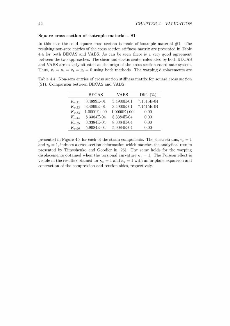
42 CHAPTER 4. VALIDATION
Square cross section of isotropic material - S1
In this case the solid square cross section is made of isotropic material #1. Theresulting non-zero entries of the cross section stiffness matrix are presented in Table4.4 for both BECAS and VABS. As can be seen there is a very good agreementbetween the two approaches. The shear and elastic center calculated by both BECASand VABS are exactly situated at the origo of the cross section coordinate system.Thus, xs = ys = xt = yt = 0 using both methods. The warping displacements are
Table 4.4: Non-zero entries of cross section stiffness matrix for square cross section(S1). Comparison between BECAS and VABS
BECAS VABS Diff. (%)
Ks,11 3.4899E-01 3.4900E-01 7.1515E-04Ks,22 3.4899E-01 3.4900E-01 7.1515E-04Ks,33 1.0000E+00 1.0000E+00 0.00Ks,44 8.3384E-04 8.3384E-04 0.00Ks,55 8.3384E-04 8.3384E-04 0.00Ks,66 5.9084E-04 5.9084E-04 0.00
presented in Figure 4.3 for each of the strain components. The shear strains, τx = 1and τy = 1, induces a cross section deformation which matches the analytical resultspresented by Timoshenko and Goodier in [26]. The same holds for the warpingdisplacements obtained when the torsional curvature κz = 1. The Poisson effect isvisible in the results obtained for κx = 1 and κy = 1 with an in-plane expansion andcontraction of the compression and tension sides, respectively.
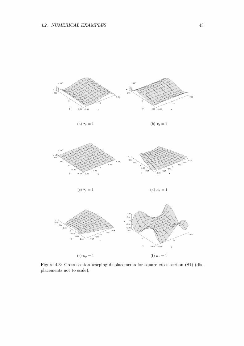
4.2. NUMERICAL EXAMPLES 43
−0.05
0
0.05
−0.05
0
0.05−5
05
x 10−3
xy
z
(a) τx = 1
−0.05
0
0.05
−0.05
0
0.05−5
05
x 10−3
xy
z(b) τy = 1
−0.04
−0.02
0
0.02
0.04
−0.04
−0.02
0
0.02
0.04−101
x 10−3
z
xy
(c) τz = 1
−0.06−0.04
−0.020
0.020.04
0.06
−0.04
−0.02
0
0.02
0.04
z
xy
(d) κx = 1
−0.04−0.02
00.02
0.04
−0.06
−0.04
−0.02
0
0.02
0.04
0.06
z
xy
(e) κy = 1
−0.05
0
0.05
−0.05
0
0.05
−0.02
−0.01
0
0.01
0.02
xy
z
(f) κz = 1
Figure 4.3: Cross section warping displacements for square cross section (S1) (dis-placements not to scale).
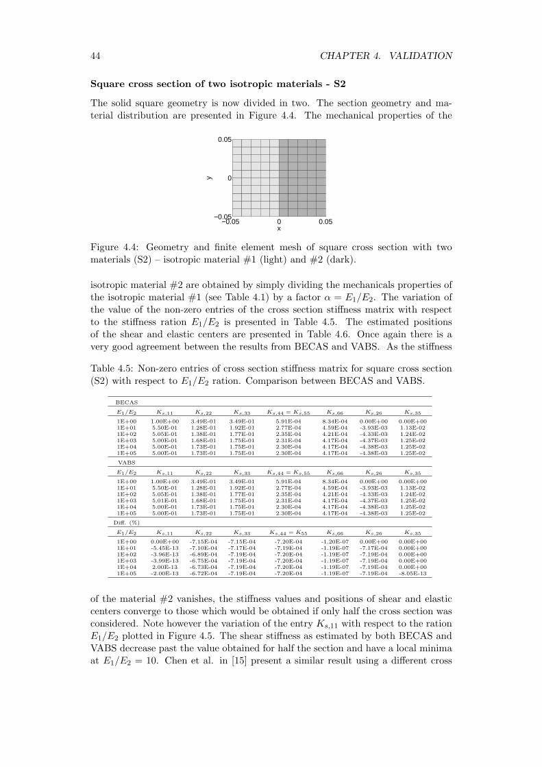
44 CHAPTER 4. VALIDATION
Square cross section of two isotropic materials - S2
The solid square geometry is now divided in two. The section geometry and ma-terial distribution are presented in Figure 4.4. The mechanical properties of the
−0.05 0 0.05−0.05
0
0.05
x
y
Figure 4.4: Geometry and finite element mesh of square cross section with twomaterials (S2) – isotropic material #1 (light) and #2 (dark).
isotropic material #2 are obtained by simply dividing the mechanicals properties ofthe isotropic material #1 (see Table 4.1) by a factor α = E1/E2. The variation ofthe value of the non-zero entries of the cross section stiffness matrix with respectto the stiffness ration E1/E2 is presented in Table 4.5. The estimated positionsof the shear and elastic centers are presented in Table 4.6. Once again there is avery good agreement between the results from BECAS and VABS. As the stiffness
Table 4.5: Non-zero entries of cross section stiffness matrix for square cross section(S2) with respect to E1/E2 ration. Comparison between BECAS and VABS.
BECAS
E1/E2 Ks,11 Ks,22 Ks,33 Ks,44 = Ks,55 Ks,66 Ks,26 Ks,35
1E+00 1.00E+00 3.49E-01 3.49E-01 5.91E-04 8.34E-04 0.00E+00 0.00E+001E+01 5.50E-01 1.28E-01 1.92E-01 2.77E-04 4.59E-04 -3.93E-03 1.13E-021E+02 5.05E-01 1.38E-01 1.77E-01 2.35E-04 4.21E-04 -4.33E-03 1.24E-021E+03 5.00E-01 1.68E-01 1.75E-01 2.31E-04 4.17E-04 -4.37E-03 1.25E-021E+04 5.00E-01 1.73E-01 1.75E-01 2.30E-04 4.17E-04 -4.38E-03 1.25E-021E+05 5.00E-01 1.73E-01 1.75E-01 2.30E-04 4.17E-04 -4.38E-03 1.25E-02
VABS
E1/E2 Ks,11 Ks,22 Ks,33 Ks,44 = Ks,55 Ks,66 Ks,26 Ks,35
1E+00 1.00E+00 3.49E-01 3.49E-01 5.91E-04 8.34E-04 0.00E+00 0.00E+001E+01 5.50E-01 1.28E-01 1.92E-01 2.77E-04 4.59E-04 -3.93E-03 1.13E-021E+02 5.05E-01 1.38E-01 1.77E-01 2.35E-04 4.21E-04 -4.33E-03 1.24E-021E+03 5.01E-01 1.68E-01 1.75E-01 2.31E-04 4.17E-04 -4.37E-03 1.25E-021E+04 5.00E-01 1.73E-01 1.75E-01 2.30E-04 4.17E-04 -4.38E-03 1.25E-021E+05 5.00E-01 1.73E-01 1.75E-01 2.30E-04 4.17E-04 -4.38E-03 1.25E-02
Diff. (%)
E1/E2 Ks,11 Ks,22 Ks,33 Ks,44 = K55 Ks,66 Ks,26 Ks,35
1E+00 0.00E+00 -7.15E-04 -7.15E-04 -7.20E-04 -1.20E-07 0.00E+00 0.00E+001E+01 -5.45E-13 -7.10E-04 -7.17E-04 -7.19E-04 -1.19E-07 -7.17E-04 0.00E+001E+02 -3.96E-13 -6.89E-04 -7.19E-04 -7.20E-04 -1.19E-07 -7.19E-04 0.00E+001E+03 -3.99E-13 -6.75E-04 -7.19E-04 -7.20E-04 -1.19E-07 -7.19E-04 0.00E+001E+04 2.00E-13 -6.73E-04 -7.19E-04 -7.20E-04 -1.19E-07 -7.19E-04 0.00E+001E+05 -2.00E-13 -6.72E-04 -7.19E-04 -7.20E-04 -1.19E-07 -7.19E-04 -8.05E-13
of the material #2 vanishes, the stiffness values and positions of shear and elasticcenters converge to those which would be obtained if only half the cross section wasconsidered. Note however the variation of the entry Ks,11 with respect to the rationE1/E2 plotted in Figure 4.5. The shear stiffness as estimated by both BECAS andVABS decrease past the value obtained for half the section and have a local minimaat E1/E2 = 10. Chen et al. in [15] present a similar result using a different cross
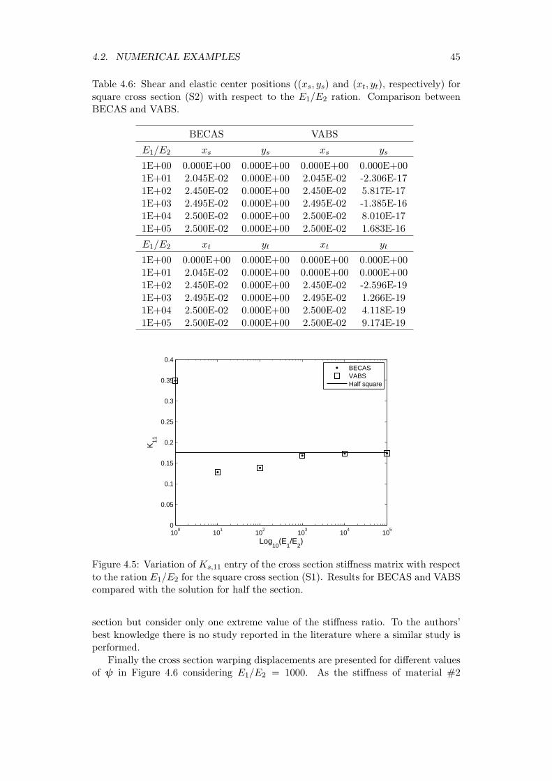
4.2. NUMERICAL EXAMPLES 45
Table 4.6: Shear and elastic center positions ((xs, ys) and (xt, yt), respectively) forsquare cross section (S2) with respect to the E1/E2 ration. Comparison betweenBECAS and VABS.
BECAS VABS
E1/E2 xs ys xs ys
1E+00 0.000E+00 0.000E+00 0.000E+00 0.000E+001E+01 2.045E-02 0.000E+00 2.045E-02 -2.306E-171E+02 2.450E-02 0.000E+00 2.450E-02 5.817E-171E+03 2.495E-02 0.000E+00 2.495E-02 -1.385E-161E+04 2.500E-02 0.000E+00 2.500E-02 8.010E-171E+05 2.500E-02 0.000E+00 2.500E-02 1.683E-16
E1/E2 xt yt xt yt
1E+00 0.000E+00 0.000E+00 0.000E+00 0.000E+001E+01 2.045E-02 0.000E+00 0.000E+00 0.000E+001E+02 2.450E-02 0.000E+00 2.450E-02 -2.596E-191E+03 2.495E-02 0.000E+00 2.495E-02 1.266E-191E+04 2.500E-02 0.000E+00 2.500E-02 4.118E-191E+05 2.500E-02 0.000E+00 2.500E-02 9.174E-19
100
101
102
103
104
105
0
0.05
0.1
0.15
0.2
0.25
0.3
0.35
0.4
Log10
(E1/E
2)
K11
BECASVABSHalf square
Figure 4.5: Variation of Ks,11 entry of the cross section stiffness matrix with respectto the ration E1/E2 for the square cross section (S1). Results for BECAS and VABScompared with the solution for half the section.
section but consider only one extreme value of the stiffness ratio. To the authors’best knowledge there is no study reported in the literature where a similar study isperformed.
Finally the cross section warping displacements are presented for different valuesof ψ in Figure 4.6 considering E1/E2 = 1000. As the stiffness of material #2
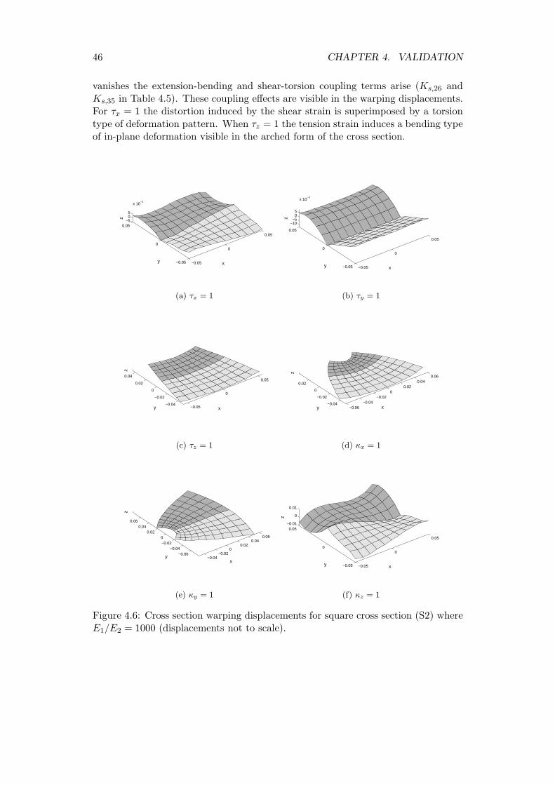
46 CHAPTER 4. VALIDATION
vanishes the extension-bending and shear-torsion coupling terms arise (Ks,26 andKs,35 in Table 4.5). These coupling effects are visible in the warping displacements.For τx = 1 the distortion induced by the shear strain is superimposed by a torsiontype of deformation pattern. When τz = 1 the tension strain induces a bending typeof in-plane deformation visible in the arched form of the cross section.
−0.05
0
0.05
−0.05
0
0.05−5
05
x 10−3
xy
z
(a) τx = 1
−0.05
0
0.05
−0.05
0
0.05
−10−5
05
x 10−3
xy
z
(b) τy = 1
−0.05
0
0.05
−0.04
−0.02
0
0.02
0.04
z
xy
(c) τz = 1
−0.06−0.04
−0.020
0.020.04
0.06
−0.04
−0.02
0
0.02
z
y x
(d) κx = 1
−0.04−0.02
00.02
0.040.06
−0.06−0.04
−0.020
0.020.04
0.06
z
xy
(e) κy = 1
−0.05
0
0.05
−0.05
0
0.05−0.01
0
0.01
xy
z
(f) κz = 1
Figure 4.6: Cross section warping displacements for square cross section (S2) whereE1/E2 = 1000 (displacements not to scale).
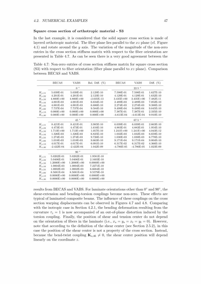
4.2. NUMERICAL EXAMPLES 47
Square cross section of orthotropic material - S3
In the last example, it is considered that the solid square cross section is made oflayered orthotropic material. The fiber plane lies parallel to the xz plane (cf. Figure4.1) and rotate around the y axis. The variation of the magnitude of the non-zeroentries in the cross section stiffness matrix with respect to the fiber orientation arepresented in Table 4.7. As can be seen there is a very good agreement between the
Table 4.7: Non-zero entries of cross section stiffness matrix for square cross section(S3) with respect to fiber orientation (fiber plane parallel to xz plane). Comparisonbetween BECAS and VABS.
BECAS VABS Rel. Diff. (%) BECAS VABS Diff. (%)
0 ◦ 22.5 ◦
Ks,11 5.039E-01 5.039E-01 2.129E-10 7.598E-01 7.598E-01 1.627E-10Ks,22 4.201E-01 4.201E-01 2.123E-10 4.129E-01 4.129E-01 1.632E-10Ks,33 4.800E+00 4.800E+00 -2.035E-13 3.435E+00 3.435E+00 7.482E-11Ks,44 4.001E-03 4.001E-03 6.634E-10 2.489E-03 2.489E-03 7.052E-10Ks,55 4.001E-03 4.001E-03 6.686E-10 2.274E-03 2.274E-03 9.388E-10Ks,66 7.737E-04 7.737E-04 9.584E-10 9.499E-04 9.499E-04 9.845E-10Ks,13 0.000E+00 0.000E+00 0.000E+00 7.387E-01 7.387E-01 2.335E-10Ks,46 0.000E+00 0.000E+00 0.000E+00 -4.613E-04 -4.613E-04 9.910E-10
45 ◦ 67.5 ◦
Ks,11 8.421E-01 8.421E-01 3.985E-10 6.039E-01 6.039E-01 2.663E-10Ks,22 4.473E-01 4.473E-01 1.616E-10 4.883E-01 4.883E-01 1.954E-10Ks,33 1.713E+00 1.713E+00 1.057E-10 1.241E+00 1.241E+00 4.043E-12Ks,44 1.326E-03 1.326E-03 6.825E-10 1.032E-03 1.032E-03 6.659E-10Ks,55 1.274E-03 1.274E-03 9.726E-10 1.030E-03 1.030E-03 6.778E-10Ks,66 1.018E-03 1.018E-03 9.663E-10 9.171E-04 9.171E-04 9.804E-10Ks,13 4.017E-01 4.017E-01 6.091E-10 6.317E-02 6.317E-02 4.366E-10Ks,46 -2.422E-04 -2.422E-04 1.042E-09 -4.786E-05 -4.786E-05 1.023E-09
90 ◦
Ks,11 5.0202E-01 5.0202E-01 1.9581E-10Ks,22 5.0406E-01 5.0406E-01 2.1603E-10Ks,33 1.2000E+00 1.2000E+00 0.0000E+00Ks,44 1.0004E-03 1.0004E-03 7.2271E-10Ks,55 1.0002E-03 1.0002E-03 6.6684E-10Ks,66 8.5081E-04 8.5081E-04 9.5579E-10Ks,13 0.0000E+00 0.0000E+00 0.0000E+00Ks,46 0.0000E+00 0.0000E+00 0.0000E+00
results from BECAS and VABS. For laminate orientations other than 0◦ and 90◦, theshear-extension and bending-torsion couplings become non-zero. These effects aretypical of laminated composite beams. The influence of these couplings on the crosssection warping displacements can be observed in Figures 4.7 and 4.8. Comparingwith the isotropic case in Section 4.2.1, the bending deformation resulting from thecurvature τz = 1 is now accompanied of an out-of-plane distortion induced by thetorsion coupling. Finally, the position of shear and tension center do not dependon the orientation of fibers in the laminate (i.e., xs = ys = xt = yt = 0). However,note that according to the definition of the shear center (see Section 2.5.2), in thiscase the position of the shear center is not a property of the cross section. Instead,because the bend-twist coupling Ks,46 6= 0, the shear center position will dependlinearly on the coordinate z.
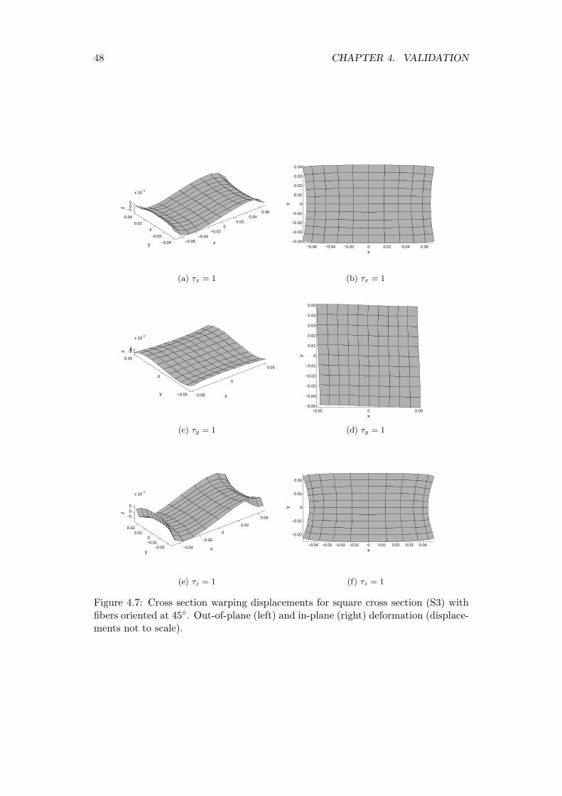
48 CHAPTER 4. VALIDATION
−0.06−0.04
−0.020
0.020.04
0.06
−0.04
−0.02
0
0.02
0.04
−505
x 10−3
xy
z
(a) τx = 1
−0.06 −0.04 −0.02 0 0.02 0.04 0.06−0.04
−0.03
−0.02
−0.01
0
0.01
0.02
0.03
0.04
x
y
(b) τx = 1
−0.05
0
0.05
−0.05
0
0.05
−202
x 10−3
xy
z
(c) τy = 1
−0.05 0 0.05−0.05
−0.04
−0.03
−0.02
−0.01
0
0.01
0.02
0.03
0.04
0.05
x
y
(d) τy = 1
−0.04
−0.02
0
0.02
0.04
−0.02−0.010
0.010.02
−505
x 10−3
xy
z
(e) τz = 1
−0.04 −0.03 −0.02 −0.01 0 0.01 0.02 0.03 0.04
−0.02
−0.01
0
0.01
0.02
x
y
(f) τz = 1
Figure 4.7: Cross section warping displacements for square cross section (S3) withfibers oriented at 45◦. Out-of-plane (left) and in-plane (right) deformation (displace-ments not to scale).

4.2. NUMERICAL EXAMPLES 49
−0.06−0.04
−0.020
0.020.04
0.06
−0.05
0
0.05
−0.01
0
0.01
xy
z
(a) κx = 1
−0.06 −0.04 −0.02 0 0.02 0.04 0.06
−0.05
−0.04
−0.03
−0.02
−0.01
0
0.01
0.02
0.03
0.04
0.05
x
y
(b) κx = 1
−0.04−0.02
00.02
0.04
−0.06
−0.04
−0.02
0
0.02
0.04
0.06
−10−5
05
x 10−3
xy
z
(c) κy = 1
−0.04 −0.02 0 0.02 0.04−0.06
−0.04
−0.02
0
0.02
0.04
0.06
x
y
(d) κy = 1
−0.05
0
0.05
−0.04
−0.02
0
0.02
0.04
−0.01
0
0.01
xy
z
(e) κz = 1
−0.05 0 0.05
−0.04
−0.03
−0.02
−0.01
0
0.01
0.02
0.03
0.04
0.05
x
y
(f) κz = 1
Figure 4.8: (continuation) Cross section warping displacements for square crosssection (S3) with fibers oriented at 45◦. Out-of-plane (left) and in-plane (right)deformation (displacements not to scale).
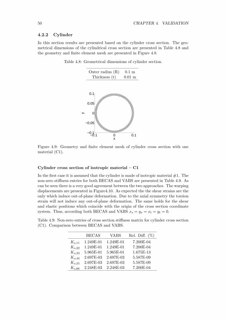
50 CHAPTER 4. VALIDATION
4.2.2 Cylinder
In this section results are presented based on the cylinder cross section. The geo-metrical dimensions of the cylindrical cross section are presented in Table 4.8 andthe geometry and finite element mesh are presented in Figure 4.8.
Table 4.8: Geometrical dimensions of cylinder section.
Outer radius (R) 0.1 mThickness (t) 0.01 m
−0.1 0 0.1−0.1
−0.05
0
0.05
0.1
x
y
Figure 4.9: Geometry and finite element mesh of cylinder cross section with onematerial (C1).
Cylinder cross section of isotropic material – C1
In the first case it is assumed that the cylinder is made of isotropic material #1. Thenon-zero stiffness entries for both BECAS and VABS are presented in Table 4.9. Ascan be seen there is a very good agreement between the two approaches. The warpingdisplacements are presented in Figure4.10. As expected the the shear strains are theonly which induce out-of-plane deformation. Due to the axial symmetry the torsionstrain will not induce any out-of-plane deformation. The same holds for the shearand elastic positions which coincide with the origin of the cross section coordinatesystem. Thus, according both BECAS and VABS xs = ys = xt = yt = 0.
Table 4.9: Non-zero entries of cross section stiffness matrix for cylinder cross section(C1). Comparison between BECAS and VABS.
BECAS VABS Rel. Diff. (%)
Ks,11 1.249E-01 1.249E-01 7.200E-04Ks,22 1.249E-01 1.249E-01 7.200E-04Ks,33 5.965E-01 5.965E-01 1.675E-13Ks,44 2.697E-03 2.697E-03 5.587E-09Ks,55 2.697E-03 2.697E-03 5.587E-09Ks,66 2.248E-03 2.248E-03 7.200E-04
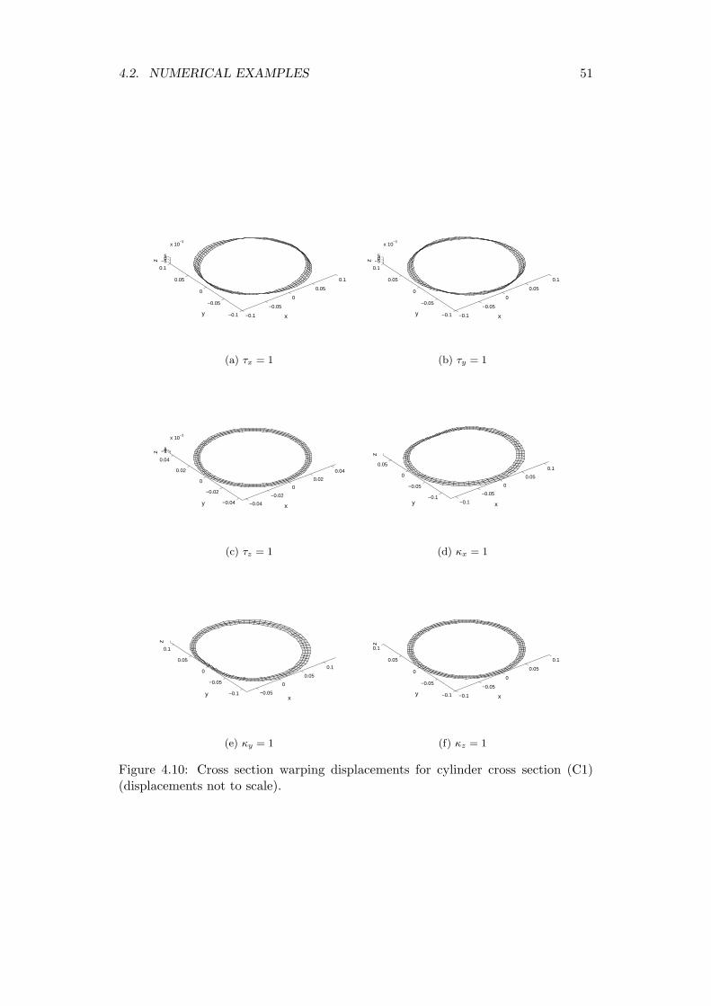
4.2. NUMERICAL EXAMPLES 51
−0.1
−0.05
0
0.05
0.1
−0.1
−0.05
0
0.05
0.1−50
5
x 10−3
xy
z
(a) τx = 1
−0.1
−0.05
0
0.05
0.1
−0.1
−0.05
0
0.05
0.1−50
5
x 10−3
xy
z(b) τy = 1
−0.04
−0.02
0
0.02
0.04
−0.04
−0.02
0
0.02
0.04
−101
x 10−3
z
xy
(c) τz = 1
−0.1
−0.05
0
0.05
0.1
−0.1
−0.05
0
0.05
z
xy
(d) κx = 1
−0.05
0
0.05
0.1
−0.1
−0.05
0
0.05
0.1
z
xy
(e) κy = 1
−0.1
−0.05
0
0.05
0.1
−0.1
−0.05
0
0.05
0.1
xy
z
(f) κz = 1
Figure 4.10: Cross section warping displacements for cylinder cross section (C1)(displacements not to scale).
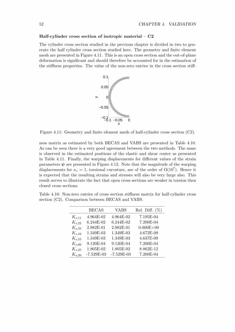
52 CHAPTER 4. VALIDATION
Half-cylinder cross section of isotropic material – C2
The cylinder cross section studied in the previous chapter is divided in two to gen-erate the half cylinder cross section studied here. The geometry and finite elementmesh are presented in Figure 4.11. This is an open cross section and the out-of-planedeformation is significant and should therefore be accounted for in the estimation ofthe stiffness properties. The value of the non-zero entries in the cross section stiff-
−0.1 −0.05 0−0.1
−0.05
0
0.05
0.1
x
y
Figure 4.11: Geometry and finite element mesh of half-cylinder cross section (C2).
ness matrix as estimated by both BECAS and VABS are presented in Table 4.10.As can be seen there is a very good agreement between the two methods. The sameis observed in the estimated positions of the elastic and shear center as presentedin Table 4.11. Finally, the warping displacements for different values of the strainparameters ψ are presented in Figure 4.12. Note that the magnitude of the warpingdisplacements for κz = 1, torsional curvature, are of the order of O(107). Hence itis expected that the resulting strains and stresses will also be very large also. Thisresult serves to illustrate the fact that open cross sections are weaker in torsion thenclosed cross sections.
Table 4.10: Non-zero entries of cross section stiffness matrix for half-cylinder crosssection (C2). Comparison between BECAS and VABS.
BECAS VABS Rel. Diff. (%)
Ks,11 4.964E-02 4.964E-02 7.195E-04Ks,22 6.244E-02 6.244E-02 7.200E-04Ks,33 2.982E-01 2.982E-01 0.000E+00Ks,44 1.349E-03 1.349E-03 4.672E-09Ks,55 1.349E-03 1.349E-03 4.637E-09Ks,66 9.120E-04 9.120E-04 7.200E-04Ks,35 1.805E-02 1.805E-02 8.862E-12Ks,26 -7.529E-03 -7.529E-03 7.200E-04
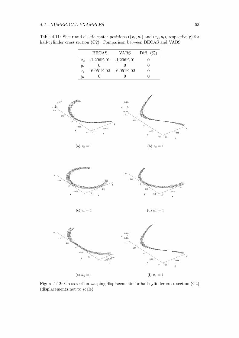
4.2. NUMERICAL EXAMPLES 53
Table 4.11: Shear and elastic center positions ((xs, ys) and (xt, yt), respectively) forhalf-cylinder cross section (C2). Comparison between BECAS and VABS.
BECAS VABS Diff. (%)
xs -1.206E-01 -1.206E-01 0ys 0. 0 0xt -6.051E-02 -6.051E-02 0yt 0. 0 0
−0.1
−0.05
0
−0.1
−0.05
0
0.05
0.1
−4−202
x 10−3
x
y
z
(a) τx = 1
−0.1
−0.05
0
−0.1
−0.05
0
0.05
0.1
−0.02
0
0.02
x
y
z
(b) τy = 1
−0.1
−0.05
0
−0.05
0
0.05
z
xy
(c) τz = 1
−0.1
−0.05
0
−0.1
−0.05
0
0.05
z
xy
(d) κx = 1
−0.06−0.04
−0.02−0.1
−0.05
0
0.05
0.1
z
x
y
(e) κy = 1
−0.1
−0.05
0
−0.1
−0.05
0
0.05
0.1
−0.010
0.01
x
y
z
(f) κz = 1
Figure 4.12: Cross section warping displacements for half-cylinder cross section (C2)(displacements not to scale).
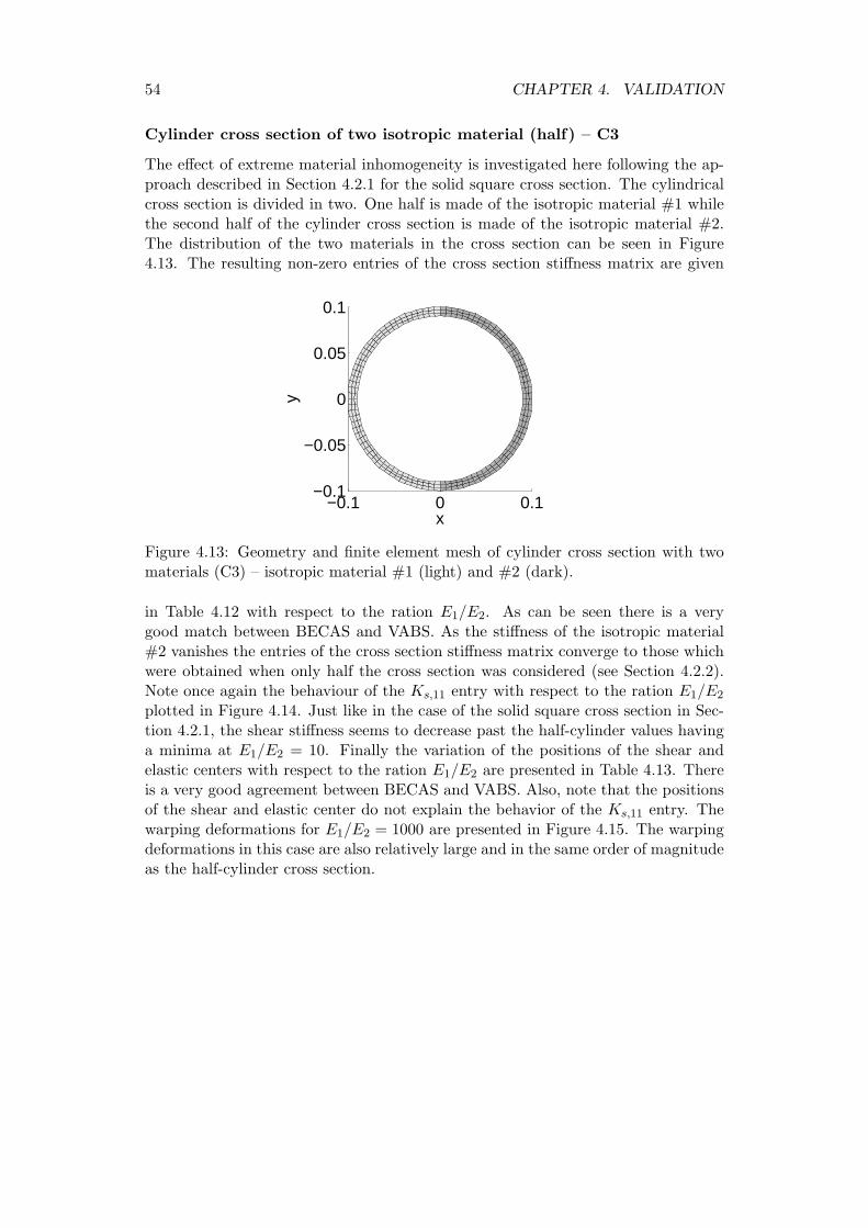
54 CHAPTER 4. VALIDATION
Cylinder cross section of two isotropic material (half) – C3
The effect of extreme material inhomogeneity is investigated here following the ap-proach described in Section 4.2.1 for the solid square cross section. The cylindricalcross section is divided in two. One half is made of the isotropic material #1 whilethe second half of the cylinder cross section is made of the isotropic material #2.The distribution of the two materials in the cross section can be seen in Figure4.13. The resulting non-zero entries of the cross section stiffness matrix are given
−0.1 0 0.1−0.1
−0.05
0
0.05
0.1
x
y
Figure 4.13: Geometry and finite element mesh of cylinder cross section with twomaterials (C3) – isotropic material #1 (light) and #2 (dark).
in Table 4.12 with respect to the ration E1/E2. As can be seen there is a verygood match between BECAS and VABS. As the stiffness of the isotropic material#2 vanishes the entries of the cross section stiffness matrix converge to those whichwere obtained when only half the cross section was considered (see Section 4.2.2).Note once again the behaviour of the Ks,11 entry with respect to the ration E1/E2
plotted in Figure 4.14. Just like in the case of the solid square cross section in Sec-tion 4.2.1, the shear stiffness seems to decrease past the half-cylinder values havinga minima at E1/E2 = 10. Finally the variation of the positions of the shear andelastic centers with respect to the ration E1/E2 are presented in Table 4.13. Thereis a very good agreement between BECAS and VABS. Also, note that the positionsof the shear and elastic center do not explain the behavior of the Ks,11 entry. Thewarping deformations for E1/E2 = 1000 are presented in Figure 4.15. The warpingdeformations in this case are also relatively large and in the same order of magnitudeas the half-cylinder cross section.
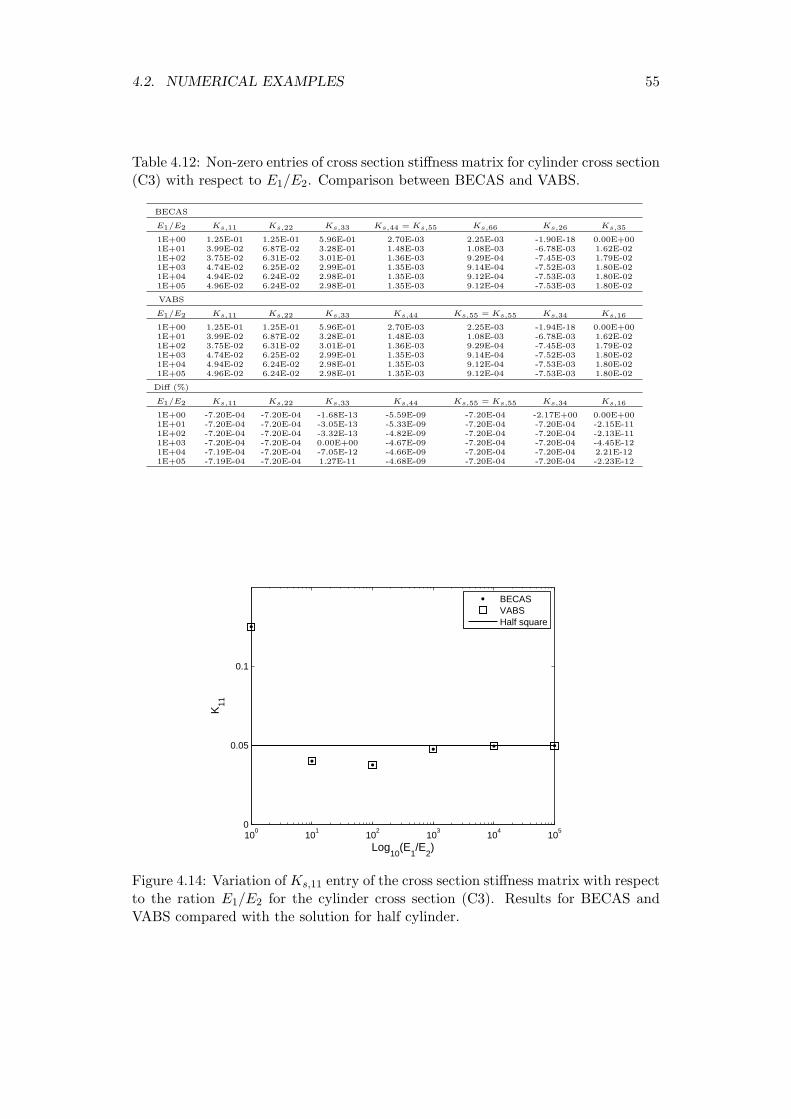
4.2. NUMERICAL EXAMPLES 55
Table 4.12: Non-zero entries of cross section stiffness matrix for cylinder cross section(C3) with respect to E1/E2. Comparison between BECAS and VABS.
BECAS
E1/E2 Ks,11 Ks,22 Ks,33 Ks,44 = Ks,55 Ks,66 Ks,26 Ks,35
1E+00 1.25E-01 1.25E-01 5.96E-01 2.70E-03 2.25E-03 -1.90E-18 0.00E+001E+01 3.99E-02 6.87E-02 3.28E-01 1.48E-03 1.08E-03 -6.78E-03 1.62E-021E+02 3.75E-02 6.31E-02 3.01E-01 1.36E-03 9.29E-04 -7.45E-03 1.79E-021E+03 4.74E-02 6.25E-02 2.99E-01 1.35E-03 9.14E-04 -7.52E-03 1.80E-021E+04 4.94E-02 6.24E-02 2.98E-01 1.35E-03 9.12E-04 -7.53E-03 1.80E-021E+05 4.96E-02 6.24E-02 2.98E-01 1.35E-03 9.12E-04 -7.53E-03 1.80E-02
VABS
E1/E2 Ks,11 Ks,22 Ks,33 Ks,44 Ks,55 = Ks,55 Ks,34 Ks,16
1E+00 1.25E-01 1.25E-01 5.96E-01 2.70E-03 2.25E-03 -1.94E-18 0.00E+001E+01 3.99E-02 6.87E-02 3.28E-01 1.48E-03 1.08E-03 -6.78E-03 1.62E-021E+02 3.75E-02 6.31E-02 3.01E-01 1.36E-03 9.29E-04 -7.45E-03 1.79E-021E+03 4.74E-02 6.25E-02 2.99E-01 1.35E-03 9.14E-04 -7.52E-03 1.80E-021E+04 4.94E-02 6.24E-02 2.98E-01 1.35E-03 9.12E-04 -7.53E-03 1.80E-021E+05 4.96E-02 6.24E-02 2.98E-01 1.35E-03 9.12E-04 -7.53E-03 1.80E-02
Diff (%)
E1/E2 Ks,11 Ks,22 Ks,33 Ks,44 Ks,55 = Ks,55 Ks,34 Ks,16
1E+00 -7.20E-04 -7.20E-04 -1.68E-13 -5.59E-09 -7.20E-04 -2.17E+00 0.00E+001E+01 -7.20E-04 -7.20E-04 -3.05E-13 -5.33E-09 -7.20E-04 -7.20E-04 -2.15E-111E+02 -7.20E-04 -7.20E-04 -3.32E-13 -4.82E-09 -7.20E-04 -7.20E-04 -2.13E-111E+03 -7.20E-04 -7.20E-04 0.00E+00 -4.67E-09 -7.20E-04 -7.20E-04 -4.45E-121E+04 -7.19E-04 -7.20E-04 -7.05E-12 -4.66E-09 -7.20E-04 -7.20E-04 2.21E-121E+05 -7.19E-04 -7.20E-04 1.27E-11 -4.68E-09 -7.20E-04 -7.20E-04 -2.23E-12
100
101
102
103
104
105
0
0.05
0.1
Log10
(E1/E
2)
K11
BECASVABSHalf square
Figure 4.14: Variation of Ks,11 entry of the cross section stiffness matrix with respectto the ration E1/E2 for the cylinder cross section (C3). Results for BECAS andVABS compared with the solution for half cylinder.
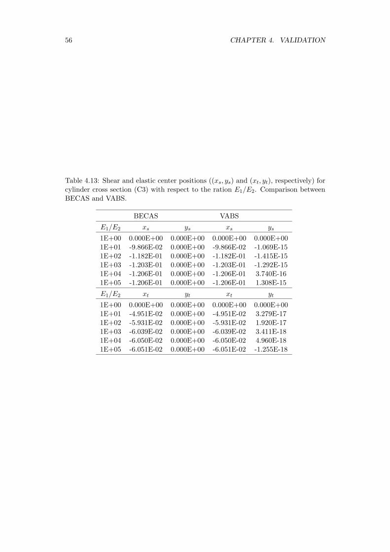
56 CHAPTER 4. VALIDATION
Table 4.13: Shear and elastic center positions ((xs, ys) and (xt, yt), respectively) forcylinder cross section (C3) with respect to the ration E1/E2. Comparison betweenBECAS and VABS.
BECAS VABS
E1/E2 xs ys xs ys
1E+00 0.000E+00 0.000E+00 0.000E+00 0.000E+001E+01 -9.866E-02 0.000E+00 -9.866E-02 -1.069E-151E+02 -1.182E-01 0.000E+00 -1.182E-01 -1.415E-151E+03 -1.203E-01 0.000E+00 -1.203E-01 -1.292E-151E+04 -1.206E-01 0.000E+00 -1.206E-01 3.740E-161E+05 -1.206E-01 0.000E+00 -1.206E-01 1.308E-15
E1/E2 xt yt xt yt
1E+00 0.000E+00 0.000E+00 0.000E+00 0.000E+001E+01 -4.951E-02 0.000E+00 -4.951E-02 3.279E-171E+02 -5.931E-02 0.000E+00 -5.931E-02 1.920E-171E+03 -6.039E-02 0.000E+00 -6.039E-02 3.411E-181E+04 -6.050E-02 0.000E+00 -6.050E-02 4.960E-181E+05 -6.051E-02 0.000E+00 -6.051E-02 -1.255E-18
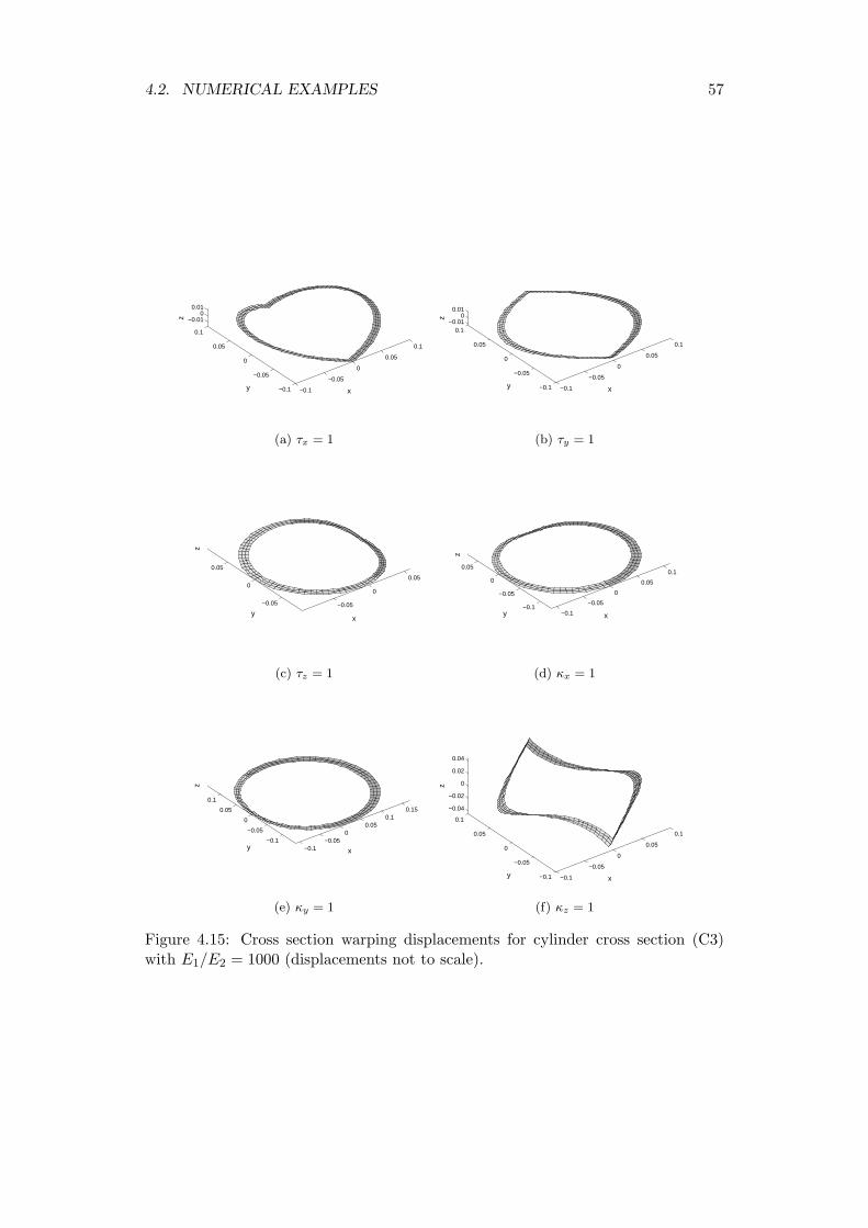
4.2. NUMERICAL EXAMPLES 57
−0.1
−0.05
0
0.05
0.1
−0.1
−0.05
0
0.05
0.1
−0.010
0.01
xy
z
(a) τx = 1
−0.1
−0.05
0
0.05
0.1
−0.1
−0.05
0
0.05
0.1−0.01
00.01
xy
z(b) τy = 1
−0.05
0
0.05
−0.05
0
0.05
z
xy
(c) τz = 1
−0.1
−0.05
0
0.05
0.1
−0.1
−0.05
0
0.05
z
xy
(d) κx = 1
−0.1−0.05
00.05
0.10.15
−0.1
−0.05
0
0.05
0.1
z
xy
(e) κy = 1
−0.1
−0.05
0
0.05
0.1
−0.1
−0.05
0
0.05
0.1
−0.04
−0.02
0
0.02
0.04
xy
z
(f) κz = 1
Figure 4.15: Cross section warping displacements for cylinder cross section (C3)with E1/E2 = 1000 (displacements not to scale).
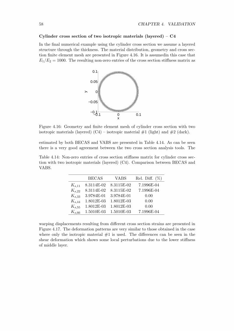
58 CHAPTER 4. VALIDATION
Cylinder cross section of two isotropic materials (layered) – C4
In the final numerical example using the cylinder cross section we assume a layeredstructure through the thickness. The material distribution, geometry and cross sec-tion finite element mesh are presented in Figure 4.16. It is assumedin this case thatE1/E2 = 1000. The resulting non-zero entries of the cross section stiffness matrix as
−0.1 0 0.1−0.1
−0.05
0
0.05
0.1
x
y
Figure 4.16: Geometry and finite element mesh of cylinder cross section with twoisotropic materials (layered) (C4) – isotropic material #1 (light) and #2 (dark).
estimated by both BECAS and VABS are presented in Table 4.14. As can be seenthere is a very good agreement between the two cross section analysis tools. The
Table 4.14: Non-zero entries of cross section stiffness matrix for cylinder cross sec-tion with two isotropic materials (layered) (C4). Comparison between BECAS andVABS.
BECAS VABS Rel. Diff. (%)
Ks,11 8.3114E-02 8.3115E-02 7.1996E-04Ks,22 8.3114E-02 8.3115E-02 7.1996E-04Ks,33 3.9784E-01 3.9784E-01 0.00Ks,44 1.8012E-03 1.8012E-03 0.00Ks,55 1.8012E-03 1.8012E-03 0.00Ks,66 1.5010E-03 1.5010E-03 7.1996E-04
warping displacements resulting from different cross section strains are presented inFigure 4.17. The deformation patterns are very similar to those obtained in the casewhere only the isotropic material #1 is used. The differences can be seen in theshear deformation which shows some local perturbations due to the lower stiffnessof middle layer.
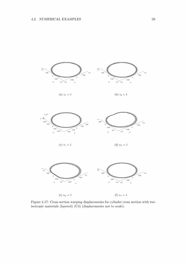
4.2. NUMERICAL EXAMPLES 59
−0.1
−0.05
0
0.05
0.1
−0.1
−0.05
0
0.05
0.1
xy
z
(a) τx = 1
−0.1
−0.05
0
0.05
0.1
−0.1
−0.05
0
0.05
0.1
xy
z
(b) τy = 1
−0.02−0.01
00.01
0.02
−0.02
−0.01
0
0.01
0.02
−101
x 10−3
z
xy
(c) τz = 1
−0.1
−0.05
0
0.05
0.1
−0.1
−0.05
0
0.05
z
xy
(d) κx = 1
−0.05
0
0.05
0.1
−0.1
−0.05
0
0.05
0.1
z
xy
(e) κy = 1
−0.1
−0.05
0
0.05
0.1
−0.1
−0.05
0
0.05
0.1
xy
z
(f) κz = 1
Figure 4.17: Cross section warping displacements for cylinder cross section with twoisotropic materials (layered) (C4) (displacements not to scale).
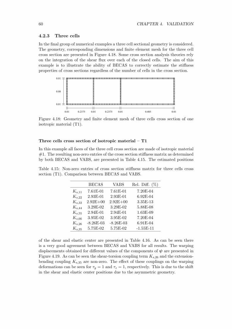
60 CHAPTER 4. VALIDATION
4.2.3 Three cells
In the final group of numerical examples a three cell sectional geometry is considered.The geometry, corresponding dimensions and finite element mesh for the three cellcross section are presented in Figure 4.18. Some cross section analysis theories relyon the integration of the shear flux over each of the closed cells. The aim of thisexample is to illustrate the ability of BECAS to correctly estimate the stiffnessproperties of cross sections regardless of the number of cells in the cross section.
0.01
0.01
0.08
0.01 0.01 0.01 0.010.2375 0.2375 0.485
Figure 4.18: Geometry and finite element mesh of three cells cross section of oneisotropic material (T1).
Three cells cross section of isotropic material – T1
In this example all faces of the three cell cross section are made of isotropic material#1. The resulting non-zero entries of the cross section stiffness matrix as determinedby both BECAS and VABS, are presented in Table 4.15. The estimated positions
Table 4.15: Non-zero entries of cross section stiffness matrix for three cells crosssection (T1). Comparison between BECAS and VABS.
BECAS VABS Rel. Diff. (%)
Ks,11 7.61E-01 7.61E-01 7.20E-04Ks,22 2.93E-01 2.93E-01 6.92E-04Ks,33 2.92E+00 2.92E+00 3.35E-13Ks,44 3.29E-02 3.29E-02 5.88E-08Ks,55 2.94E-01 2.94E-01 1.63E-09Ks,66 3.95E-02 3.95E-02 7.20E-04Ks,26 -8.26E-03 -8.26E-03 6.91E-04Ks,35 5.75E-02 5.75E-02 -1.55E-11
of the shear and elastic center are presented in Table 4.16. As can be seen thereis a very good agreement between BECAS and VABS for all results. The warpingdisplacements obtained for different values of the components of ψ are presented inFigure 4.19. As can be seen the shear-torsion coupling term Ks,26 and the extension-bending coupling Ks,35 are non-zero. The effect of these couplings on the warpingdeformations can be seen for τy = 1 and τz = 1, respectively. This is due to the shiftin the shear and elastic center positions due to the asymmetric geometry.
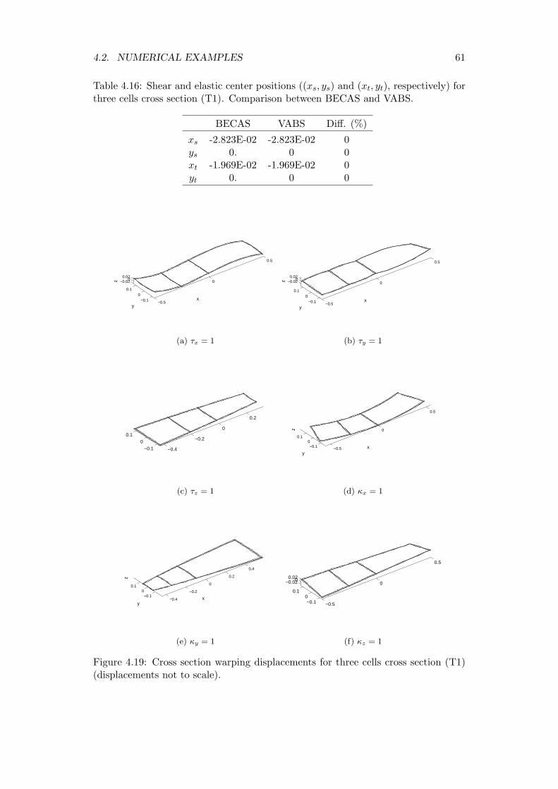
4.2. NUMERICAL EXAMPLES 61
Table 4.16: Shear and elastic center positions ((xs, ys) and (xt, yt), respectively) forthree cells cross section (T1). Comparison between BECAS and VABS.
BECAS VABS Diff. (%)
xs -2.823E-02 -2.823E-02 0ys 0. 0 0xt -1.969E-02 -1.969E-02 0yt 0. 0 0
−0.5
0
0.5
−0.10
0.1
−0.020
0.02
x
y
z
(a) τx = 1
−0.5
0
0.5
−0.10
0.1
−0.020
0.02
x
y
z
(b) τy = 1
−0.4
−0.2
0
0.2
−0.10
0.1
(c) τz = 1
−0.5
0
0.5
−0.10
0.1
z
yx
(d) κx = 1
−0.4
−0.2
0
0.2
0.4
−0.10
0.1
z
yx
(e) κy = 1
−0.5
0
0.5
−0.10
0.1
−0.0200.02
(f) κz = 1
Figure 4.19: Cross section warping displacements for three cells cross section (T1)(displacements not to scale).

62 CHAPTER 4. VALIDATION
Three cells cross section of orthotropic top faces and isostropic webs - T2
In the last numerical experiment the top faces of the three cells cross section arelaminated using the orthotropic material oriented at 45◦. The vertical faces are madeof isotropic material. The material distribution is visible in Figure 4.20. The aim is
−0.5 0 0.5
−0.1
0
0.1
x
y
Figure 4.20: Geometry and finite element mesh of three cells cross section withorthotropic material at 45◦ in the top faces (dark) and isotropic material in thevertical shear webs (light) T2.
to combine in one experiment the effects of material anisotropy and inhomogeneityusing a closed thin-walled multi-cell cross section. The non-zero entries of the crosssection stiffness matrix as estimated by BECAS and VABS are presented in Table4.17. As can be seen there is a very good agreement between both methods. Theresulting positions of the shear and elastic center are presented in Table 4.18. Likebefore, both BECAS and VABS present a very good agreement in the estimation ofthe shear and elastic center.
Table 4.17: Non-zero entries of cross section stiffness matrix for three cells crosssection with orthotropic material at 45◦ in the top faces and isotropic material inthe vertical webs (T2).
BECAS VABS Rel. Diff. (%)
Ks,11 1.79E+00 1.79E+00 1.36E-10Ks,22 3.22E-01 3.22E-01 2.13E-09Ks,33 4.37E+00 4.37E+00 2.98E-11Ks,44 5.23E-02 5.23E-02 2.16E-10Ks,55 3.81E-01 3.81E-01 1.21E-10Ks,66 7.73E-02 7.73E-02 3.29E-10Ks,31 -8.48E-01 -8.48E-01 1.13E-10Ks,35 5.64E-02 5.64E-02 -3.88E-11Ks,15 2.75E-03 2.75E-03 6.11E-09Ks,26 -1.49E-02 -1.49E-02 2.42E-09Ks,24 -3.13E-03 -3.13E-03 2.16E-09Ks,64 1.83E-02 1.83E-02 5.79E-10
4.2. NUMERICAL EXAMPLES 63
Table 4.18: Shear and elastic center positions ((xs, ys) and (xt, yt), respectively) forthree cells cross section T2. Comparison between BECAS and VABS.
BECAS VABS Diff. (%)
xs -4.300E-02 -4.300E-02 0ys 0. 0 0xt -1.456E-02 -1.456E-02 0yt 0. 0 0
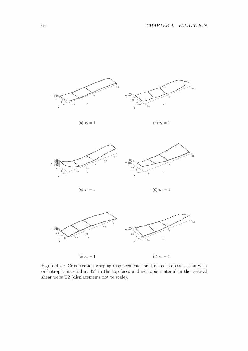
64 CHAPTER 4. VALIDATION
−0.5
0
0.5
−0.10
0.1
−0.0100.01
x
y
z
(a) τx = 1
−0.5
0
0.5
−0.10
0.1
−0.0200.02
xy
z(b) τy = 1
−0.4
−0.2
0
0.2
0.4
−0.10
0.1
−0.04−0.02
00.020.040.06
x
y
z
(c) τz = 1
−0.5
0
0.5
−0.10
0.1
−0.04−0.0200.020.04
xy
z
(d) κx = 1
−0.4
−0.2
0
0.2
0.4
−0.10
0.1
−0.02−0.0100.01
xy
z
(e) κy = 1
−0.5
0
0.5
−0.10
0.1
−0.0200.02
xy
z
(f) κz = 1
Figure 4.21: Cross section warping displacements for three cells cross section withorthotropic material at 45◦ in the top faces and isotropic material in the verticalshear webs T2 (displacements not to scale).
Chapter 5
User’s Manual
The usage of BECAS is described in this chapter. The aim is to go through thefunctionalities of BECAS and discuss its practical usage within a structural analysisenvironment. BECAS is implemented as a Matlab toolbox. The following functionsare available
• BECAS_Utils - Build arrays for BECAS calculations.
• BECAS_Constitutive_Ks - Calculation of the cross section stiffness matrix;
• BECAS_Constitutive_Ms - Calculation of the cross section mass matrix;
• BECAS_CrossSectionProps - Calculation of the cross section properties;
• BECAS_RecoverStrains - Calculation of the three-dimensional strains at eachpoint in the cross section;
• BECAS_RecoverStresses - Calculation of the three-dimensional stresses ateach point in the cross section;
• BECAS_TransformationMat - Rotate and translate the cross section constitu-tive matrices;
• BECAS_Becas2Hawc2 - Generate output for latest version of Hawc2.
• BECAS_3D_Utils - Build working arrays for BECAS calculations.
• BECAS_3D_Constitutive_Ks - Calculation of the cross section stiffness matrixbased on solid finite element models of the cross section;
• BECAS_3D_CrossSectionProps - Calculation of the cross section properties;
The version of BECAS based on two-dimensional finite element discretizations of thecross section is presented first. The use of the BECAS_3D tool is discussed last inSection 5.3.
Note that the BECAS toolbox also includes a number of functions for visualiza-tion of the input and output. The description of this functions has been omitted asit falls beyond the scope of theis manual.
Part of the MATLAB code in BECAS is generated through MAPLE. There arefour MAPLE files which follow together with the BECAS code:
65
66 CHAPTER 5. USER’S MANUAL
• GenerateMatricesBECAS.mw used to generate all the element stiffness matriceswhich are included in the MATLAB function Quad4 used within the functionBECAS_Constitutive_Ks.
• LayerRotationBECAS.mw used to generate the code for the function which ro-tates the material constitutive matrixQ in the MATLAB function BECAS_Utilswhen orienting the fibers in a layer.
• FiberPlaneRotationBECAS.mw used to generate the code for the functionwhich rotates the material constitutive matrix Q when orienting the fiberplane in an element in the MATLAB function BECAS_Utils.
5.1 Input
In order to run BECAS the following input is necessary:
• nl_2d - (nn×3) array with the list of nodal positions where each row is in theform (node number, x coordinate, y coordinate), where nn is the total numberof nodes. The node numbering need not be in any specific order.
• el_2d - (ne × 8) array with the element connectivity table where each row isin the form (element number, node 1, node 2, node 3, node 4, node 5, node6, node 7, node 8 ), where ne is the total number of elements. The elementnumbering need not be in any specific order. The value of node 5 throughnode 8 has to be zero for Quad4 element to be used. Otherwise, Quad8 isautomatically chosen.
• emat - (ne × 4) array with element material properties assignment where eachrow is in the form (element number, material number, fiber angle, fiber planeangle), where ne is the total number of elements. The element numberingneed not be in any specific order. The material number corresponds to thematerials assigned in the matprops array.
• matprops - (nmat× 10) array with the material properties where each row isin the form (E11, E22, E33, G12, G13, G23, ν12, ν13, ν23, ), where nmat isthe total number of different materials considered. The material mechanicalproperties given with respect to the material coordinate system have been aredefined as
– E11 the Young modulus of material the 1 direction.
– E22 the Young modulus of material the 2 direction.
– E33 the Young modulus of material the 3 direction.
– G12 the shear modulus in the 12 plane.
– G13 the shear modulus in the 13 plane.
– G23 the shear modulus in the 23 plane.
– ν12 the Poisson’s ratio in the 12 plane.
– ν13 the Poisson’s ratio in the 13 plane.

5.2. LIST OF FUNCTIONS AND OUTPUT 67
– ν23 the Poisson’s ratio in the 23 plane.
– the material density.
The rotation of the material constitutive tensor is described in Section 3.2.
5.1.1 Example
All the files necessary to run all the examples presented for the Validation in Section4 are distributed together with BECAS. These files can be used as a starting pointfor the development of new input for BECAS.
5.2 List of functions and output
The different functions included in the BECAS library and corresponding outputare described in this chapter.
5.2.1 BECAS_Utils
The function BECAS_Utils is used to build working arrays. It is included inside allthe other functions in the 2D version of BECAS. It is called using
[utils]=BECAS_Utils(nl_2d,el_2d,emat,matprops)
5.2.2 BECAS_Constitutive_Ks
The function BECAS_Constitutive_Ks is the BECAS central function and is usedprimarily for the evaluation of the cross section stiffness matrix Ks. The function iscalled using
[Ks,dX,dY,X,Y]=BECAS_Constitutive_Ks(nl_2d,el_2d,emat,matprops);
The output is
• Ks - (6× 6) array storing the cross section stiffness matrix Ks.
• dX - (nd × 6) array ∂X∂z .
• dY - (6× 6) array ∂Y∂z .
• X - (nd × 6) array X.
• Y - (6× 6) array Y.
where nd = nn×3 is the number of degrees of freedom in cross section finite elementequations.
5.2.3 BECAS_Constitutive_Ms
The function BECAS_Constitutive_Ms is used for the evaluation of the cross sectionmass matrix Ms. It is called as
[Ms]=BECAS_Constitutive_Ms(nl_2d,el_2d,emat,matprops);
The output is
• Ms - (6× 6) array storing the cross section mass matrix Ms.
68 CHAPTER 5. USER’S MANUAL
5.2.4 BECAS_CrossSectionProps
The function BECAS_CrossSectionProps is used to determine a series of relevantcross section properties. It presumes that the cross section stiffness Ks has beenpreviously determined. The function is called using
[ ShearX,ShearY,ElasticX,ElasticY,...
MassX,MassY,MassPerUnitLength,...
AlphaPrincipleAxis,AlphaPrincipleAxis_ElasticCenter,...
AreaX,AreaY,AreaTotal,...
Ixx,Iyy,Ixy,Axx,Ayy,Axy]=...
BECAS_CrossSectionProps(Ks,nl_2d,el_2d,emat,matprops);
The output is
• ShearX - the xs position of the cross section shear center.
• ShearY - the ys position of the cross section shear center.
• ElasticX - the xt position of the cross section elastic center.
• ElasticY - the yt position of the cross section elastic center.
• MassX - the xm position of the cross section mass center.
• MassY - the ym position of the cross section mass center.
• MassPerUnitLength - the cross section mass per unit length.
• AlphaPrincipleAxis - the orientation of the cross section elastic axis deter-mined at the reference point (in radians).
• AlphaPrincipleAxis_ElasticCenter - the orientation of the cross sectionelastic center determined at the elastic center (in radians).
• AreaX - the x coordinate of the area centroid.
• AreaY - the y coordinate of the area centroid.
• AreaTotal - total cross section area.
• Ixx - the mass moment of inertia with respect to the x axis.
• Iyy - the mass moment of inertia with respect to the y axis.
• Ixy - the mass product of inertia.
• Axx - the area moment of inertia with respect to the x axis.
• Ayy - the area moment of inertia with respect to the y axis.
• Axy - the area product of inertia.
5.2. LIST OF FUNCTIONS AND OUTPUT 69
5.2.5 BECAS_RecoverStrains
The function BECAS_RecoverStresses is used to determine the three-dimensionalstrains components at the center of each element and at each Gauss point in thecross section finite element mesh. The function is meant to be used after the one-dimensional beam finite element solution has been determined. The resulting strainvalues are given in the global coordinate systems. The function is called as
[ElementStrain_GlobalCS,NodalStrain_GlobalCS]=...
BECAS_RecoverStrains(theta0,dX,dY,X,Y,nl_2d,el_2d,emat,matprops);
Part of the input is coming from the BECAS_Constitutive_Ks function. The extrainput consists of
• theta0 - (1×6) array holding the cross section generalized forces and moments
(i.e., the variable θ =[TT MT
]Tdefined in Section 2.2.1). The magnitude of
the entries are generally determined based on the one-dimensional beam finiteelement solution.
The output is
• ElementStrain_GlobalCS - (6×ne) array holding the three-dimensional straincomponents evaluated at the center of each of the elements in the cross sectionfinite element mesh.
• NodalStrain_GlobalCS - ((6×ngp)×ne) array holding the three-dimensionalstrain components evaluated at the each of the Gauss points (ngp Gauss pointsat each element) in the cross section finite element mesh.
Note: function is not yet validated.
5.2.6 BECAS_RecoverStresses
The function BECAS_RecoverStress is used to determine the three-dimensionalstress components at each element or at each Gauss point in the cross section finiteelement mesh. The function is meant to be used after the one-dimensional beamfinite element solution has been determined. The stresses are evaluated based on thestrains determined using the BECAS_RecoverStrains. The resulting stress valuesare given in both the global and material coordinate systems. The function is calledas
[ElementStress_GlobalCS,ElementStress_MaterialCS,...
NodalStress_GlobalCS,NodalStress_MaterialCS] = ...
BECAS_RecoverStress(ElementStrain_GlobalCS,...
NodalStrain_GlobalCS,nl_2d,el_2d,emat,matprops);
The output is
• ElementStress_GlobalCS - (6×ne) array holding the three-dimensional stresscomponents in the global coordinate system evaluated at the center of each ofthe elements in the cross section finite element mesh.
70 CHAPTER 5. USER’S MANUAL
• ElementStress_MaterialCS - (6 × ne) array holding the three-dimensionalstress components in the local coordinate system evaluated at the center ofeach of the elements in the cross section finite element mesh.
• NodalStress_GlobalCS - ((6×ngp)×ne) array holding the three-dimensionalstrain components in the global coordinate system evaluated at the each ofthe Gauss points (where ngp are the number of Gauss points at each element)in the cross section finite element mesh.
• NodalStress_MaterialCS - ((6×ngp)×ne) array holding the three-dimensionalstrain components in the material coordinate system evaluated at the each ofthe Gauss points (where ngp are the number of Gauss points at each element)in the cross section finite element mesh..
Note: function is not yet validated.
5.2.7 BECAS_Becas2Hawc2
The function BECAS_Becas2Hawc2 is used to generate input for RISØ’s HAWC2code for the aeroelastic analysis of wind turbines. It is presumed that the functionsBECAS_Constitutive_Ks, BECAS_Constitutive_Ms, and BECAS_CrossSectionPropshave been previously called. Extra input is required for this function, namely, thefollowing have to be defined:
• RadialPosition - coordinate of the section along the span of the blade.
• OutputFilename - name of file to which the output is written (e.g., OutputFilename= ’BECAS2HAWC2.out’ ).
The function is called as
BECAS_Becas2Hawc2(OutputFilename,RadialPosition,...
Ks,Ms,...
ShearX,ShearY,...
ElasticX,ElasticY,...
MassX,MassY,...
AlphaPrincipleAxis_ElasticCenter,...
AreaX,AreaY,AreaTotal,...
Axx,Ayy,Axy,...
nl_2d,el_2d,emat,matprops)
5.2.8 BECAS_TransformMat
The function BECAS_TransformMat is used to determine the translated and rotatedvalues of the cross section constitutive stiffness or mass matrices. The functionrequires extra input, namely:
• p - column array specifying the coordinates of the new reference point (e.g.,p = [ShearX ShearY] to translate the matrix to the shear center).
5.3. THE BECAS 3D IMPLEMENTATION 71
• alpha - angle of rotation around the z axis, in degrees, defined positive in thecounter-clockwise direction (e.g., alpha=AlphaPrincipleAxis to align withthe elastic axis).
The function is called as
[M]=BECAS_TransformationMat(M,p,alpha);
5.2.9 Examples
All the files required for the replication of the validation examples are distributedtogether with BECAS. The user should specify the name of the corresponding folderin the file Inputdata4RunMe.m. The file RunMe.m which calls BECAS should then beran to obtain the results.
5.3 The BECAS 3D implementation
An alternative implementation of BECAS using solid finite elements is described here.The main advantage of this approach concerns the possibility of using layered solidfinite elements. All BECAS functions associated with this implementation start byBECAS_3D.
5.3.1 Input
The input to the BECAS_3D group of functions is
• k3d - nd × 3 array with the sparse form of stiffness matrix of the cross sectionslice meshed with solid finite elements, where nd is the number of degrees offreedom in the solid finite element model. Each row in the k3d array is inthe form (row number, column number, value), where row and column numbercorrespond to the row and column positions in the global stiffness matrix.
• nl_3d - nn,3d×3 array with the list of nodal positions where each row is in theform (node number, x coordinate, y coordinate, z coordinate), where nn,3d is thetotal number of nodes in the solid finite element model. The node numberingneeds to be in the same order as it is listed in the k3d matrix.
5.3.2 List of functions and output
The following functions are part of the BECAS_3D group of functions.
5.3.3 BECAS_3D_Utils
The function BECAS_3D_Utils is used to build working arrays. It is included insideall the other functions in the 3D version of BECAS. It is called using
[utils] = BECAS_3D_Utils(k3d,n3d);
72 CHAPTER 5. USER’S MANUAL
5.3.4 BECAS_3D_Constitutive_Ks
This is the main function of the BECAS_3d and is used to determine the cross sectionstiffness matrix Ks. It is called using
[Ks,dX,dY,X,Y]=BECAS_3D_Constitutive_Ks(k3d,n3d);d
The output is
• Ks - (6× 6) array storing the cross section stiffness matrix Ks.
• dX - (nd × 6) array ∂X∂z .
• dY - (6× 6) array ∂Y∂z .
• X - (nd × 6) array X.
• Y - (6× 6) array Y.
where nd = nn×3 is the number of degrees of freedom in cross section finite elementequations.
5.3.5 BECAS_3D_CrossSectionProps
The function BECAS_3D_CrossSectionProps returns some relevant cross sectionproperties. It presumes that the cross section stiffness matrix Ks has been pre-viously determined. The function is called through
[ShearX,ShearY,ElasticX,ElasticY,AlphaPrincipleAxis]=...
BECAS_3D_CrossSectionProps(Ks);
The output is
• ShearX - the xs position of the cross section shear center.
• ShearY - the ys position of the cross section shear center.
• ElasticX - the xt position of the cross section elastic center.
• ElasticY - the yt position of the cross section elastic center.
• MassX - the xm position of the cross section mass center.
• MassY - the ym position of the cross section mass center.
• MassPerUnitLength - the cross section mass per unit length.
• AlphaPrincipleAxis - the orientation of the cross section elastic
Bibliography
[1] Ganguli R., Chopra I., Aeroelastic optimization of a helicopter rotor with com-posite coupling, Journal of Aircraft, 32(6), 1326-1334, 1995
[2] Li L., Volovoi V. V., Hodges D. H., Cross-sectional design of composite rotorblades, Journal of the American Helicopter Society, 53(3), 240-251, 2008
[3] Blasques J. P., Stolpe M., Maximum stiffness and minimum weight optimiza-tion of laminated composite beams using continuous fiber angles, Structural andMultidisciplinary Optimization, DOI: 10.1007/s00158-010-0592-9, 2010
[4] Hansen M. O. L., Sørensen J. N., Voutsinas S., Sørensen N., Madsen H. A.,State of the art in wind turbine aerodynamics and aeroelasticity, Progress inAerospace Sciences, (42), 285-330, 2006
[5] Chaviaropoulos, P.K., et al., Enhancing the damping of wind turbine rotorblades - the DAMPBLADE project, Wind Energy, 9, 163-177, 2006.
[6] Giavotto V., Borri M., Mantegazza P., Ghiringhelli G., Carmaschi V., MaffioluG.C., Mussi F., Anisotropic beam theory and applications, Composite Struc-tures, (16)1-4, 403-413, 1983
[7] Borri M., Merlini T., A large displacement formulation for anisotropic beamanalysis, Meccanica, (21), 30-37, 1986
[8] Borri M., Ghiringhelli G. L., Merlini T., Linear analysis of naturally curved andtwisted anisotropic beams, Composites Engineering, (2)5-7, 433-456, 1992
[9] Ghiringhelli G. L., Mantegazza P., Linear, straight and untwisted anisotropicbeam section properties from solid finite elements, (4)12, 1225-1239, 1994
[10] Ghiringhelli G. L., On the thermal problem for composite beams using a finiteelement semi-discretization, Composites Part B, (28B), 483-495, 1997
[11] Ghiringhelli G. L., On the linear three dimensional behaviour of compositebeams, Composites Part B, (28B), 613-626, 1997
[12] Ghiringhelli G. L., Masarati P., Mantegazza P.,Characterisation of Anisotropic,Non-Homogeneous Beam Sections with Embedded Piezo-Electric Materials,Journal of Intelligent Material Systems and Structures, (8)10, 842-858, 1997
[13] Yu W., Hodges D. H., Volovoi V., Cesnik C. E. S., On Timoshenko-like mod-elling of initially curved and twisted composite beams, International Journal ofSolids and Structures, (39), 5101-5121, 2002
73
74 BIBLIOGRAPHY
[14] Yu W., Volovoi, V. V., Hodges D. H., Hong X., Validation of the VariationalAsymptotic Beam Sectional Analysis (VABS), AIAA Journal, (40)10, 2105-2113, 2002
[15] Chen H., Yu W., Capellaro M., A critical assessment of computer tools forcalculating composite wind turbine blade properties, Wind Energy, (13)6, 497-516, 2010
[16] Jung S. N., Nagaraj V. T., Chopra I., Assessment of composite rotor blademodeling techniques, Journal of the American Helicopter Society, (44)3, 188-205, 1999
[17] Volovoi V. V., Hodges D. H., Cesnik C. E. S., Popescu B., Assessment of beammodeling methods for rotor blade applications, Mathematical and ComputerModeling, (33), 1099-1112, 2001
[18] Horgan C. O., On Saint-Venant’s principle in plane anisotropic elasticity, Jour-nal of Elasticity, (2)3, 169-180, 1972
[19] Choi I., Horgan C. O., Saint-Venant’s principle and end effects in anisotropicelasticity, Transactions of the ASME, 424-430, 1977
[20] Horgan C. O., Knowles J. K., Recent developments concerning Saint-Venant’sprinciple, Advances in Applied Mechanics, (23), 180-262, 1983
[21] Christensen O., Differentialligninger of uendelige rı¿12kker, ed. Institut for
Matematik, Danmarks Tekniske Universitet, 30-32, 2009
[22] Hogdes D. H., Nonlinear composite beam theory, Progress in Astronautics andAeronautics, (213), 2006
[23] Bendsøe, M.P., Sigmund, O., Topology Optimization: Theory, Methods andApplications, 2nd Edition, Springer-Verlag, Berlin, 2003
[24] Reddy J. N., Mechanics of laminated Composite plates and shells: theory andanalysis, 2nd Edition, CRC Press, 1997
[25] Peters S. T., Handbook of composites, 2nd Edition, Chapman & Hall, London,1998
[26] Timoshenko S., Goodier J. N., Theory of elasticity, McGraw-Hill, 1951