USGS OF10-1013

Geophysical Investigations at Hidden Dam, Raymond, California: Summary of Fieldwork and Data Analysis

Open-File Report 2010–1013

U.S. Department of the Interior U.S. Geological Survey

Cover: Looking southeast across the downstream embankment of Hidden Dam, from the right abutment. Photo by Burke J. Minsley

Prepared in cooperation with the U.S. Army Corps of Engineers

Geophysical Investigations at Hidden Dam, Raymond, California: Summary of Fieldwork and Data Analysis

By Burke J. Minsley, Bethany L. Burton, Scott Ikard, and Michael H. Powers

Open-File Report 2010–1013

U.S. Department of the Interior U.S. Geological Survey

U.S. Department of the Interior KEN SALAZAR, Secretary

U.S. Geological Survey Marcia K. McNutt, Director

U.S. Geological Survey, Reston, Virginia: 2010

For product and ordering information: World Wide Web: http://www.usgs.gov/pubprod Telephone: 1-888-ASK-USGS

For more information on the USGS—the Federal source for science about the Earth, its natural and living resources, natural hazards, and the environment: World Wide Web: http://www.usgs.gov Telephone: 1-888-ASK-USGS

Suggested citation: Minsley, B.J., Burton, Bethany L., Ikard, Scott, and Powers, M.H., 2010, Geophysical investigations at Hidden Dam, Raymond, California—Summary of fieldwork and data analysis: U.S. Geological Survey Open-File Report 2010–1013, 25 p.

Any use of trade, product, or firm names is for descriptive purposes only and does not imply endorsement by the U.S. Government.

Although this report is in the public domain, permission must be secured from the individual copyright owners to reproduce any copyrighted material contained within this report.

Geophysical Investigations at Hidden Dam

iii

Contents Introduction ................................................................................................................................................................. 1 Site Background ......................................................................................................................................................... 2

Location and Geology ............................................................................................................................................. 2 Right Abutment Seepage Area................................................................................................................................ 3

Geophysical Surveys .................................................................................................................................................. 4 Self-potential ........................................................................................................................................................... 4

Data Acquisition .................................................................................................................................................. 5 Data Processing and Interpretation ..................................................................................................................... 8

DC Resistivity ........................................................................................................................................................ 11 Data Acquisition ................................................................................................................................................ 12 Data Processing and Interpretation ................................................................................................................... 14

Future Work .............................................................................................................................................................. 22 Conclusions .............................................................................................................................................................. 22 Acknowledgments ..................................................................................................................................................... 23 References Cited ...................................................................................................................................................... 24


iv

Figures 1. Location (inset) and aerial photo of Hidden Dam indicating the geophysical study area for this report ............... 2 2. Hidden Dam reservoir elevation from January 1, 1999, to present from the California Department of

Water Resources Data Exchange Center. .......................................................................................................... 3 3. Cartoon illustration of self-potential signals driven by groundwater flow. ............................................................ 5 4. Map of the self-potential survey stations (red) and telluric dipole (green). . ....................................................... 6 5. Time series of the telluric field recorded during each day of self-potential data acquisition ................................ 7 6. Histogram of all telluric data shows weak variability, typically less than 2 µV·ft-1 .............................................. 7 7. Interpolated self-potential map over the downstream portion of the survey area. ............................................... 9 8. Photograph of the outlet works area (looking northwest towards the right abutment) highlighting the

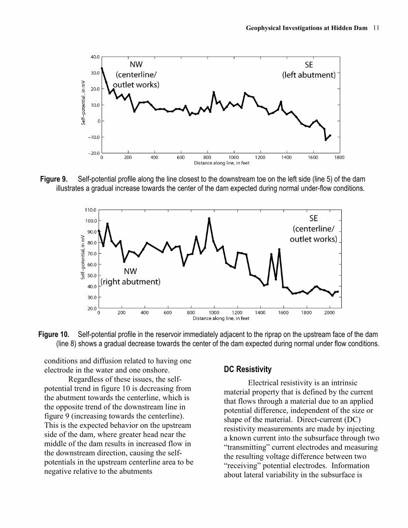
approximate extent of the self-potential anomaly at location C in figure 7 ......................................................... 10 9. Self-potential profile along the line closest to the downstream toe on the left side (line 5) of the dam

illustrates a gradual increase towards the center of the dam expected during normal under-flow conditions.... 11 10. Self-potential profile in the reservoir immediately adjacent to the riprap on the upstream face of the dam

(line 8) shows a gradual decrease towards the center of the dam expected during normal under flow conditions .......................................................................................................................................................... 11

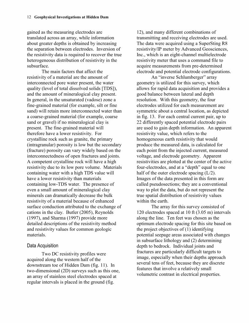
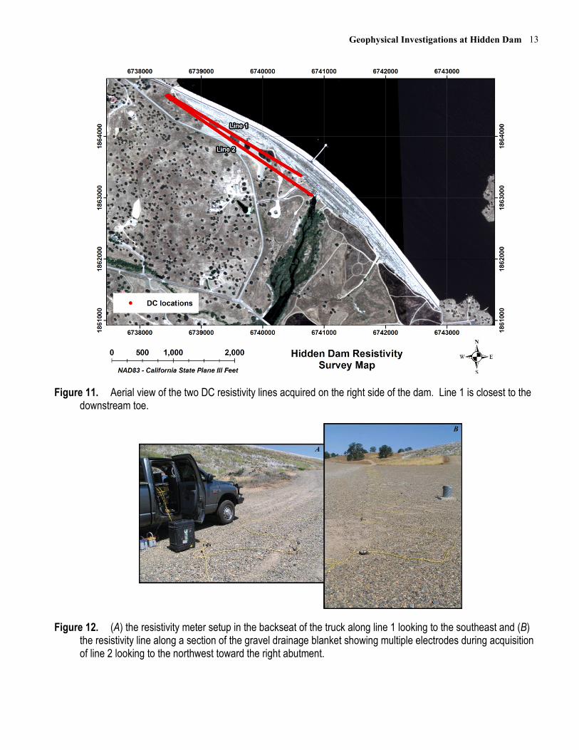
11. Map of the two DC resistivity lines acquired on the right side of the dam .......................................................... 13 12. Photos taken on the downstream side of the dam of (A) the resistivity meter setup in the backseat of the

truck along line 1 looking to the southeast and of (B) the resistivity line along a section of the gravel drainage blanket showing multiple electrodes during acquisition of line 2 looking to the northwest toward the right abutment. ............................................................................................................................................ 13

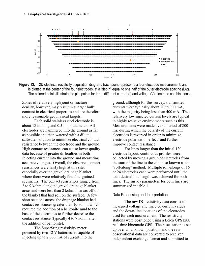
13. 2D electrical resistivity acquisition diagram: Each point represents a four-electrode measurement, and is plotted at the center of the four electrodes, at a “depth” equal to one half of the outer electrode spacing (L/2). The colored points illustrate the plot points for three different current (I) and voltage (V) electrode combinations ..................................................................................................................................................... 14

14. Data misfit crossplots for DC resistivity lines 1 and 2. The top two plots are of (A) line 1 and (B) line 2 after the first inversion run of 10 iterations. The bottom two plots are of (C) line 1 and (D) line 2 after the second inversion run after the removal of noisy data points using data misfit thresholds of 30 percent and 40 percent, resulting in the removal of 6.6 percent and 5.9 percent of the total number of data points, respectively ....................................................................................................................................................... 17

15. DC resistivity line 1 (A) measured data apparent resistivity pseudosection, (B) forward modeled apparent resistivity pseudosection, and (C) inverted resistivity section.. .......................................................................... 18

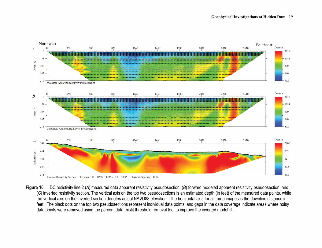
16. DC resistivity line 2 (A) measured data apparent resistivity pseudosection, (B) forward modeled apparent resistivity pseudosection, and (C) inverted resistivity section.. .......................................................................... 19

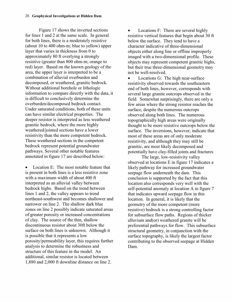
17. Inverted sections for DC resistivity (A) line 1 and (B) line 2. Location E, observed on both lines, is interpreted to be a deep alluvial valley between bedrock highs; locations F are highly resistive features that may represent competent granitic highs with complex geometry; and locations G illustrate high near-surface resistivity associated with large granite outcrops.......................................................................... 21

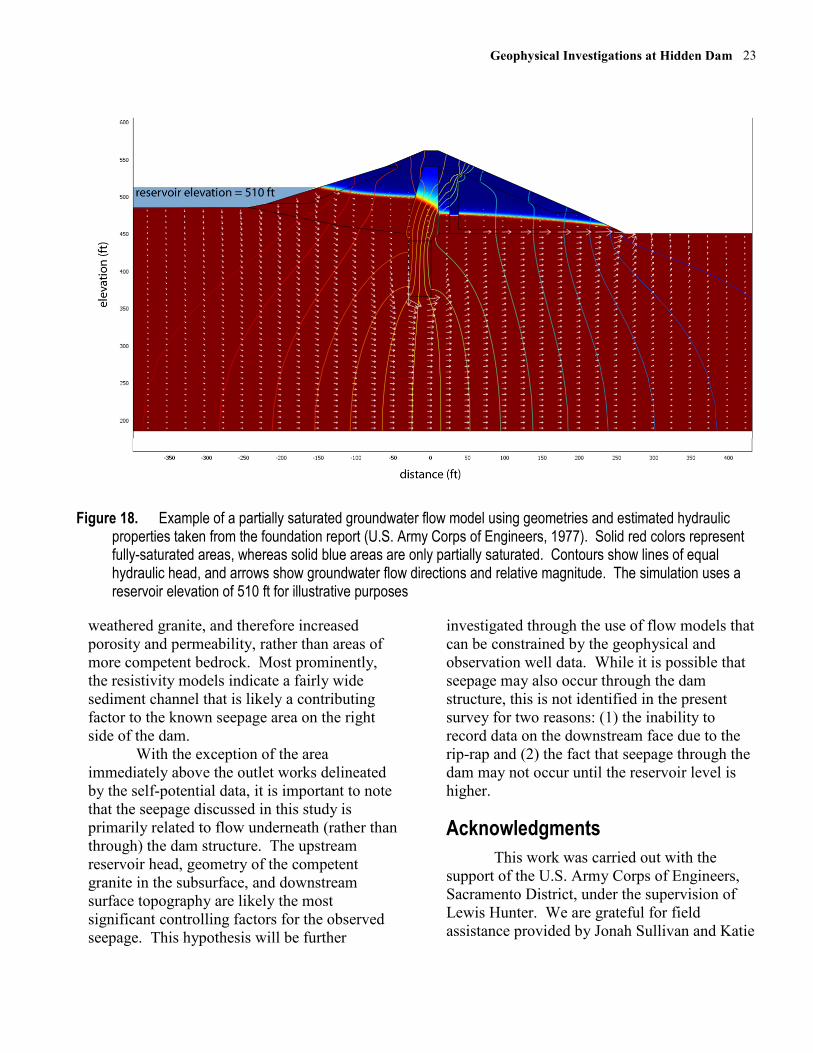
18. Example of a partially saturated groundwater flow model using geometries and estimated hydraulic properties taken from the foundation report (U.S. Army Corps of Engineers, 1977). ........................................ 23


v

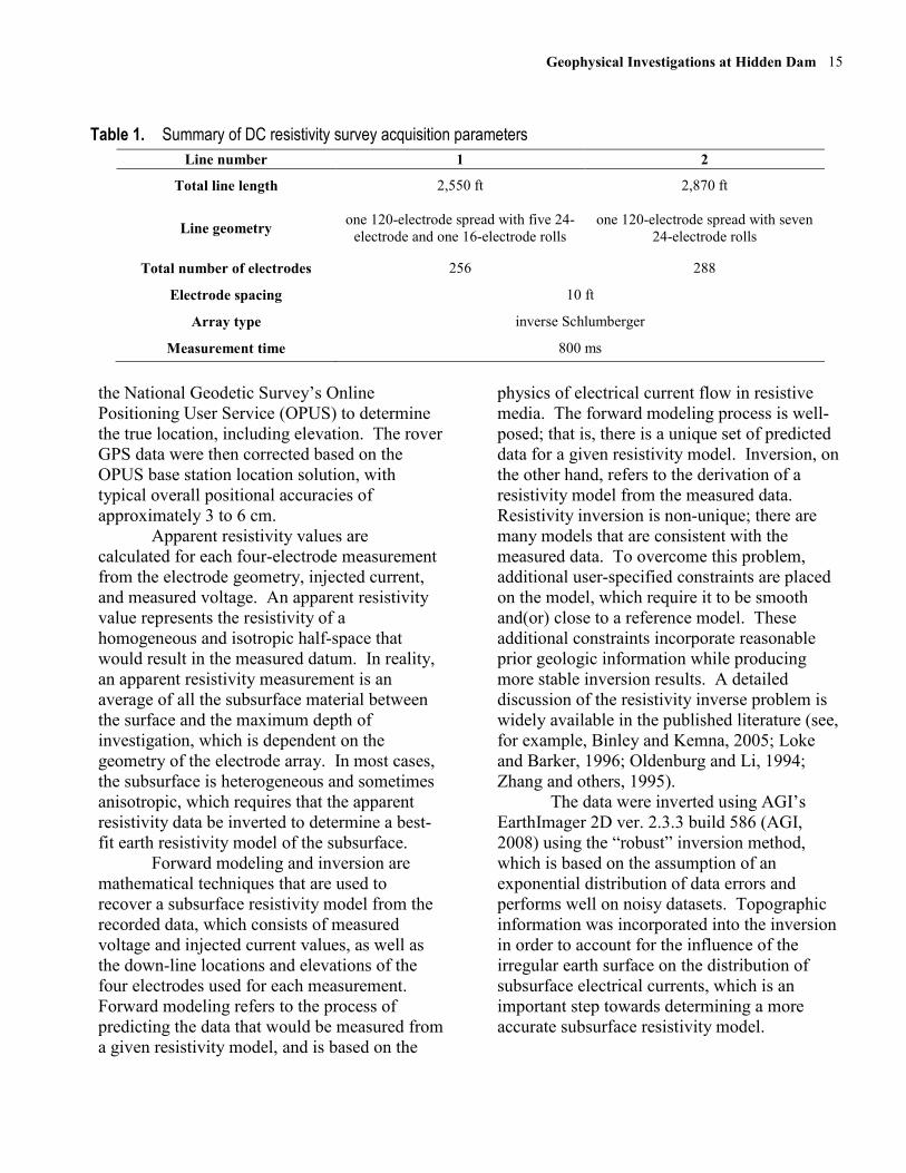
Table 1. Summary of DC resistivity survey acquisition parameters ................................................................................. 15


vi

Conversion Factors Inch/Pound to SI

Multiply By To obtain

Length

inch (in.) 2.54 centimeter (cm)

foot (ft) 0.3048 meter (m)

mile (mi) 1.609 kilometer (km)

Area

acre 4,047 square meter (m2)

acre 0.004047 square kilometer (km2)

square mile (mi2) 2.590 square kilometer (km2)

Volume

gallon (gal) 0.003785 cubic meter (m3)

acre-foot (acre-ft) 1,233 cubic meter (m3) SI to Inch/Pound


Length

centimeter (cm) 0.3937 inch (in.)

meter (m) 3.281 foot (ft)

kilometer (km) 0.6214 mile (mi)

Area

square meter (m2) 0.0002471 acre

square kilometer (km2) 247.1 acre

square kilometer (km2) 0.3861 square mile (mi2)

Volume

cubic meter (m3) 264.2 gallon (gal)

cubic meter (m3) 0.0008107 acre-foot (acre-ft) Vertical coordinate information is referenced to North American Vertical Datum of 1988 (NAVD 88). Horizontal coordinate information is referenced to the North American Datum of 1983 (NAD 83). Elevation, as used in this report, refers to distance above the vertical datum.


vii

Electrical Conductivity and Electrical Resistivity


Electrical conductivity

siemens per meter (S/m) 1,000 millisiemens per meter (mS/m)

siemens per meter (S/m) 10,000 microsiemens per meter (µS/cm)

Electrical resistivity ohm-meters (ohm-m) 0.001 kiloohm-meters (kohm-m)

Electrical conductivity σ in siemens per meter (S/m) can be converted to electrical resistivity ρ in ohm-meters (ohm-m) as follows: ρ = 1/ σ. Electrical resistivity ρ in ohm-meters (ohm-m) can be converted to electrical conductivity σ in siemens per meter (S/m) as follows: σ = 1/ ρ.

Geophysical Investigations at Hidden Dam, Raymond, CA: Summary of Fieldwork and Data Analysis

By Burke J. Minsley, Bethany L. Burton, Scott Ikard, and Michael H. Powers

Introduction Geophysical field investigations have

been carried out at the Hidden Dam in Raymond, California for the purpose of better understanding the hydrogeology and seepage-related conditions at the site. Known seepage areas on the northwest right abutment area of the downstream side of the dam are documented by Cedergren (1980a; 1980b). Subsequent to the 1980 seepage study, a drainage blanket with a subdrain system was installed to mitigate downstream seepage. Flow net analysis provided by Cedergren (1980a; 1980b) suggests that the primary seepage mechanism involves flow through the dam foundation due to normal reservoir pool elevations, which results in upflow that intersects the ground surface in several areas on the downstream side of the dam. In addition to the reservoir pool elevations and downstream surface topography, flow is also controlled by the existing foundation geology as well as the presence or absence of a horizontal drain within the downstream portion of the dam.

The purpose of the current geophysical work is to (1) identify present-day seepage areas that may not be evident due to the effectiveness of the drainage blanket in redirecting seepage water, and (2) provide information about subsurface geologic structures that may control subsurface flow and seepage. These tasks are accomplished through the use of two complementary electrical geophysical methods, self-potentials (SP) and direct-current (DC)

electrical resistivity, which have been commonly utilized in dam-seepage studies (for example, Corwin, 2007; Dahlin and others, 2008). SP is a passive method that is primarily sensitive to active subsurface groundwater flow and seepage, whereas DC resistivity is an active-source method that is sensitive to changes in subsurface lithology and groundwater saturation.

The focus of this field campaign was on the downstream area on the right abutment, or northwest side of the dam, as this is the main area of interest regarding seepage. Two exploratory self-potential lines were also collected on the downstream left abutment of the dam to identify potential seepage in that area. This report is primarily a summary of the field geophysical data acquisition, with some preliminary results and interpretation. Further work will involve a more rigorous analysis of the geophysical datasets and an examination of a large dataset of historical observations of water levels in a number of observation wells and piezometers compared with reservoir elevation. In addition, a partially saturated flow model will be developed to better understand seepage patterns given the available information about dam construction, geophysical results, and data from installed observation wells and piezometers.


2

Site Background Location and Geology

Hidden Dam is located on the Fresno River in the Sierra Nevada foothills, approximately 15 miles northeast of Madera, California (fig. 1). Detailed information regarding the dam construction and local geology and hydrology, summarized below, is provided by the U.S. Army Corps of Engineers (1977) as well as Cedergren (1980a; 1980b). Hidden Dam is a rolled earthfill dam constructed between 1972 and 1975, with a crest length of approximately 5,700 ft and a maximum height above streambed of 184 ft and a crest elevation of 561 ft. At gross pool (elevation of 540 ft), the impounded lake has a surface area of about 1,570 acres and a storage capacity of 90,000 acre-feet. Relief at the dam site is approximately 180 ft with elevations ranging between around 400 ft at the streambed to approximately 580 ft on the right and left

abutments. This topography is characterized by gently rolling, rounded hills with scattered rock outcrops.

The area in the vicinity of Hidden Dam is underlain by what is generally described as granitic and associated metamorphic rocks derived from the Sierra Nevada batholith, though there is some variability in composition, texture, and color. Granitic rocks are overlain by residual soil, slope wash, and alluvium, ranging in thickness from zero to approximately 30 ft and varying in composition between sands, silts, and clays. Beneath the overburden, to depths up to 60 ft, the granite is decomposed such that it is easily crumbled or broken. Fresh rock occurs below the decomposed granite, though decomposed materials are occasionally interspersed up to depths of 140 ft. Jointing was observed throughout the foundation area during excavation, though the profusion of joints and the extent to which they are clay-filled varies throughout the site.

Figure 1. Location (inset) and aerial photo of Hidden Dam indicating the geophysical study area for this report.


3

Right Abutment Seepage Area Observations were obtained from

sixteen piezometers initially installed at the dam site, plus fourteen additional observation wells installed as part of the seepage study. Flow net analyses calibrated to the piezometer data, and physical observations of seepage areas highlighted that the primary area of seepage concern in 1980 was on the right side of the dam. At a pool elevation of 484 ft in the 1980 study, significant total head was observed in a number of observation wells and piezometers on the right abutment, confirming areas of seepage at the toe of the dam. An important point from the analysis of the observation well data is that the pressure head relative to ground surface was positive for all wells at an elevation of 465 ft or less, while the pressure head relative to ground surface was negative for all wells at higher elevations. As the reservoir elevation decreases to 470 ft, little-to-no seepage would be expected in this area as this is approximately the elevation near the

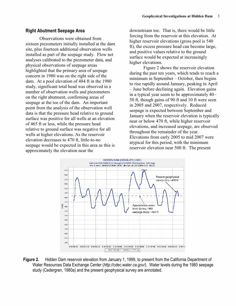
downstream toe. That is, there would be little forcing from the reservoir at this elevation. At higher reservoir elevations (gross pool is 540 ft), the excess pressure head can become large, and positive values relative to the ground surface would be expected at increasingly higher elevations.

Figure 2 shows the reservoir elevation during the past ten years, which tends to reach a minimum in September – October, then begins to rise rapidly around January, peaking in April – June before declining again. Elevation gains in a typical year seem to be approximately 40–50 ft, though gains of 90 ft and 10 ft were seen in 2005 and 2007, respectively. Reduced seepage is expected between September and January when the reservoir elevation is typically near or below 470 ft, while higher reservoir elevations, and increased seepage, are observed throughout the remainder of the year. Elevations from early 2005 to mid 2007 were atypical for this period, with the minimum reservoir elevation near 500 ft. The present

Figure 2. Hidden Dam reservoir elevation from January 1, 1999, to present from the California Department of Water Resources Data Exchange Center (http://cdec.water.ca.gov/). Water levels during the 1980 seepage study (Cedergren, 1980a) and the present geophysical survey are annotated.

http://cdec.water.ca.gov/�


4

geophysical survey was scheduled for early May in order to coincide with the seasonal maximum reservoir elevation, and therefore the greatest potential for seepage, though the 2009 high pool reservoir elevation only reached approximately 490 ft. This elevation is relatively low, though still higher than the 484 ft level recorded during the 1980 seepage study. Because the self-potential method is sensitive to active seepage, it is important to record these data during a period when seepage is expected to occur.

Geophysical Surveys Self-potential

The self-potential method measures the naturally-occurring electrical potential (voltage) on the earth surface. Self-potentials are a somewhat unique geophysical method in that they are sensitive to active processes in the subsurface, in contrast with methods such as resistivity that are sensitive to physical properties. One of the primary sources of self-potential signals is subsurface fluid flow (such as seepage); an excess positive charge that develops near grain surfaces in saturated porous geologic media is transported along with the fluid, creating a streaming current density.

This subsurface electrokinetic phenomenon generates a balancing conduction current density, which flows through the earth resistivity structure and is manifested as the measurable self-potential on the earth surface (Ishido and Mizutani, 1981; Morgan and others, 1989; Sill, 1983). The degree of coupling between fluid and electrical flows varies with fluid and rock chemistry, but is generally such that the electrical potential gradient is in the opposite direction of the hydraulic gradient. That is, increasingly positive self-potentials are typically measured in the direction of fluid flow (or decreasing hydraulic head). A seepage-related self-potential signal would therefore be positive in the downstream/outflow area, and more negative in the upstream/infiltration area.

This is illustrated conceptually in figure 3, which illustrates a typical self-potential response (top) that becomes increasingly positive in the direction of groundwater flow. Excess charge in porous media is dragged along with flow (blue line, bottom), generating a streaming electrical current. Because total electrical current must be conserved, the streaming current generates a balancing electrical conduction current (red lines) that flows throughout the earth. Self-potentials sample the electrical potential at various points on the ground surface that result from this conduction current.

Self-potentials are measured by recording the electrical potential difference between non-polarizing electrodes placed at various points on the ground surface using a high impedance (>107 ohm) voltmeter. Because measurements involve the potential difference between points, maps of self-potential values are plotted relative to a survey reference location, which is typically assigned a value of zero volts. Large areas can be covered using multiple lines of data, which must be tied together to recover the self-potential at any location relative to the survey reference (Corwin, 1990).

Sources of noise during a self-potential survey can be anthropogenic, such as grounded power lines, buried metallic structures, or cathodic protection systems, as well as naturally occurring due to geochemical variability or background telluric fields. Buried metals and cathodic protection systems typically have a characteristic negative self-potential signature that increases in magnitude with proximity to the source, and can often be recognized in the field data. In some cases this unwanted noise can be partially removed from the data, but it cannot always be perfectly separated from subtle signals at the same location. Telluric fields refer to electric currents that flow through the earth due to fluctuating currents in the ionosphere. These earth currents are associated


5

Figure 3. Self-potential signals driven by groundwater flow. Excess charge is dragged along with flow in porous media, generating a streaming electrical current (blue line) that is balanced by an electrical conduction current (red lines) that traverses the earth resistivity structure. Self-potentials measure the resulting potential difference between various points on the ground surface. Because of the nature of electrokinetic coupling, self-potentials typically become more positive in the direction of flow.

with an electrical potential field as they traverse the earth resistivity structure, and often exhibit a diurnal variability that can reach magnitudes on the order of 10 mV•km–1 (Telford and others, 1990). A telluric monitoring dipole is sometimes deployed during a self-potential survey to determine a time-varying correction that can be applied to the self-potential data (Corwin, 2005).

Data Acquisition Self-potential measurements were made

using the reference electrode method, whereby the electrical potential is measured between a fixed base electrode and a roving electrode connected to a long spool of wire (approximately 2,500 ft). Non-polarizing lead/lead chloride electrodes, fashioned after the Petiau electrode (Petiau, 2000), were used for all self-potential measurements. At each station, three shallow holes were dug and filled with a small amount of salted bentonite mud to

improve electrical contact with the earth in the generally dry and gravelly conditions found at the site. Five self-potential measurements were recorded in each of the three holes, for a total of 15 measurements per station, using an Agilent U1252A digital voltmeter and laptop computer with data logging software. Each station was assigned a unique identifier to facilitate further processing, and locations were recorded with a handheld GPS unit.

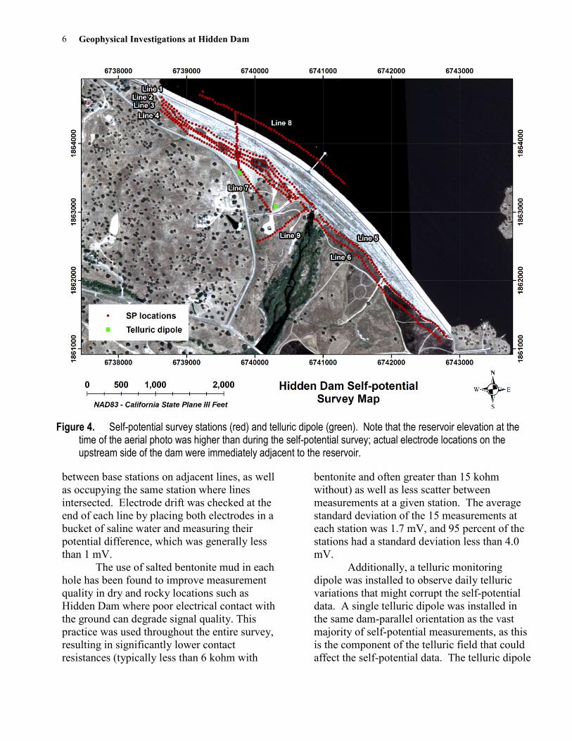
A total of 512 self-potential stations were acquired, primarily along several lines that parallel the downstream toe of the dam (fig. 4), though several other transects were also surveyed in areas of interest including one line in the reservoir on the upstream side of the dam. Individual lines of data were collected by spooling out the roving electrode at 40 ft intervals (nominal station spacing) along the line from the base electrode location. A new base electrode location was established for each line, and individual lines of data have been tied together by measuring the self-potential


6

Figure 4. Self-potential survey stations (red) and telluric dipole (green). Note that the reservoir elevation at the time of the aerial photo was higher than during the self-potential survey; actual electrode locations on the upstream side of the dam were immediately adjacent to the reservoir.

between base stations on adjacent lines, as well as occupying the same station where lines intersected. Electrode drift was checked at the end of each line by placing both electrodes in a bucket of saline water and measuring their potential difference, which was generally less than 1 mV.

The use of salted bentonite mud in each hole has been found to improve measurement quality in dry and rocky locations such as Hidden Dam where poor electrical contact with the ground can degrade signal quality. This practice was used throughout the entire survey, resulting in significantly lower contact resistances (typically less than 6 kohm with

bentonite and often greater than 15 kohm without) as well as less scatter between measurements at a given station. The average standard deviation of the 15 measurements at each station was 1.7 mV, and 95 percent of the stations had a standard deviation less than 4.0 mV.

Additionally, a telluric monitoring dipole was installed to observe daily telluric variations that might corrupt the self-potential data. A single telluric dipole was installed in the same dam-parallel orientation as the vast majority of self-potential measurements, as this is the component of the telluric field that could affect the self-potential data. The telluric dipole


7

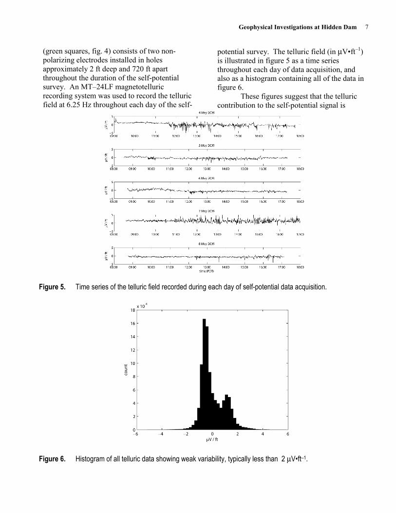
(green squares, fig. 4) consists of two non-polarizing electrodes installed in holes approximately 2 ft deep and 720 ft apart throughout the duration of the self-potential survey. An MT–24LF magnetotelluric recording system was used to record the telluric field at 6.25 Hz throughout each day of the self-

potential survey. The telluric field (in µV•ft–1) is illustrated in figure 5 as a time series throughout each day of data acquisition, and also as a histogram containing all of the data in figure 6.

These figures suggest that the telluric contribution to the self-potential signal is

Figure 5. Time series of the telluric field recorded during each day of self-potential data acquisition.

Figure 6. Histogram of all telluric data showing weak variability, typically less than 2 µV•ft–1.


8

generally weak (mostly less than 2 µV•ft–1), with no significant diurnal trend that might bias measurements over the course of a day. For the longest self-potential measurement dipole of approximately 2,500 ft, telluric noise on the order of 2 µV•ft–1 corresponds to approximately 5 mV telluric error, which is roughly equivalent to the observed survey-wide measurement error. Most measurements are made with a smaller electrode separation, and therefore contain a proportionally smaller component of telluric error. Telluric corrections are therefore not applied to the self-potential data at this point

Data Processing and Interpretation The raw self-potential data consist of

measurements of the electrical potential between the base electrode and roving electrode for each line, as well as electrode drift measurements at the end of each line. These data are processed to produce a map of the electrical potential at every station relative to a survey-wide reference location, which is chosen as the northwestern-most point in the survey next to the downstream toe on the right abutment and is assigned a value of zero mV. Measurements taken between the base stations of adjacent lines, as well as locations where two lines intersect, are critical in producing the final self-potential map because these data provide information needed to tie all of the individual lines together. The final map was generated using the procedure discussed in more detail by Minsley and others (2008), which produces a smoothly varying self-potential map that honors (1) measurements along each line, (2) errors estimated from the 15 measurements at each station, (3) electrode drift corrections, (4) a unique potential value at line intersection points, and (5) Kirchhoff’s law, which requires that the total potential drop along any closed loop equal zero.

Figure 7 shows the resulting self-potential map (in mV) relative to the survey-wide reference location in the northwest corner. The upstream data are omitted from this figure,

and are displayed separately due to the questionable quality of their tie-in values relative to the downstream data. This is likely due to poor electrical contact on the riprap along the tie-line collected over the crest of the dam, as well as differences in oxidation-reduction (redox) and electrode diffusion for the measurements where the roving electrode was placed in the reservoir. Four likely seepage-related locations are marked on figure 7 based on the expected positive self-potential values in the vicinity of seepage outflow areas.

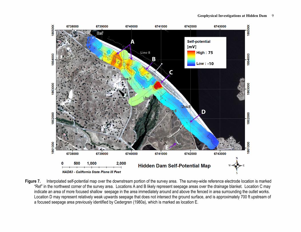
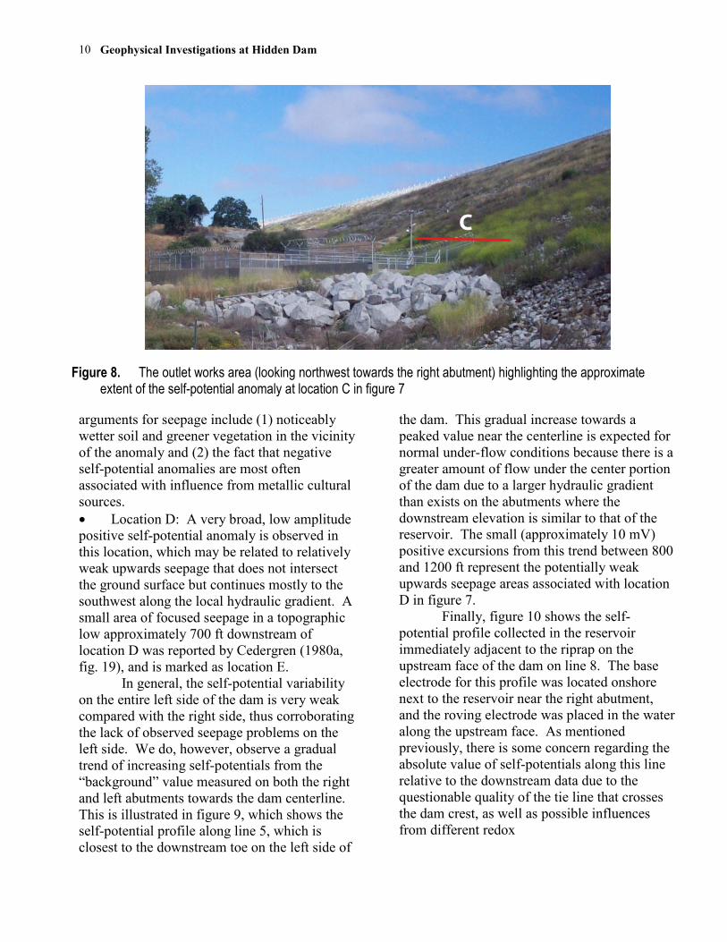
• Locations A and B: These areas of elevated self-potential are very well correlated with the known seepage areas from the 1980 study (Cedergren, 1980a, b), and therefore also with the location of the drainage blanket. The positive anomalies seem to be focused in the areas of lower topography between several mounds on the downstream side of the dam. Lower self-potential values found on top of the mounds may be due to (1) seepage being directed towards the relatively higher permeability drainage blanket and (2) increased distance from the ground surface to the seepage upflow which can attenuate the self-potential signal. • Location C: A very large (+170 mV) and spatially focused (less than approximately 50 ft wide) self-potential anomaly is observed immediately around and above the fenced in area surrounding the outlet works (fig. 8). The magnitude and peaked character of this anomaly suggest relatively focused and shallow outflow in this area. This, in addition to the fact that it is located somewhat uphill from the toe of the dam, supports the possibility that this could be related to piping or internal seepage exiting through the embankment rather than the foundation seepage associated with the location A and B seepage areas. The proximity of this anomaly to the dam outlet structure leads to some concern that it may be cultural-related, which cannot be fully discounted. However,


9

Figure 7. Interpolated self-potential map over the downstream portion of the survey area. The survey-wide reference electrode location is marked “Ref” in the northwest corner of the survey area. Locations A and B likely represent seepage areas over the drainage blanket. Location C may indicate an area of more focused shallow seepage in the area immediately around and above the fenced in area surrounding the outlet works. Location D may represent relatively weak upwards seepage that does not intersect the ground surface, and is approximately 700 ft upstream of a focused seepage area previously identified by Cedergren (1980a), which is marked as location E.


10

Figure 8. The outlet works area (looking northwest towards the right abutment) highlighting the approximate extent of the self-potential anomaly at location C in figure 7

arguments for seepage include (1) noticeably wetter soil and greener vegetation in the vicinity of the anomaly and (2) the fact that negative self-potential anomalies are most often associated with influence from metallic cultural sources. • Location D: A very broad, low amplitude positive self-potential anomaly is observed in this location, which may be related to relatively weak upwards seepage that does not intersect the ground surface but continues mostly to the southwest along the local hydraulic gradient. A small area of focused seepage in a topographic low approximately 700 ft downstream of location D was reported by Cedergren (1980a, fig. 19), and is marked as location E.

In general, the self-potential variability on the entire left side of the dam is very weak compared with the right side, thus corroborating the lack of observed seepage problems on the left side. We do, however, observe a gradual trend of increasing self-potentials from the “background” value measured on both the right and left abutments towards the dam centerline. This is illustrated in figure 9, which shows the self-potential profile along line 5, which is closest to the downstream toe on the left side of

the dam. This gradual increase towards a peaked value near the centerline is expected for normal under-flow conditions because there is a greater amount of flow under the center portion of the dam due to a larger hydraulic gradient than exists on the abutments where the downstream elevation is similar to that of the reservoir. The small (approximately 10 mV) positive excursions from this trend between 800 and 1200 ft represent the potentially weak upwards seepage areas associated with location D in figure 7.

Finally, figure 10 shows the self-potential profile collected in the reservoir immediately adjacent to the riprap on the upstream face of the dam on line 8. The base electrode for this profile was located onshore next to the reservoir near the right abutment, and the roving electrode was placed in the water along the upstream face. As mentioned previously, there is some concern regarding the absolute value of self-potentials along this line relative to the downstream data due to the questionable quality of the tie line that crosses the dam crest, as well as possible influences from different redox


11

Figure 9. Self-potential profile along the line closest to the downstream toe on the left side (line 5) of the dam illustrates a gradual increase towards the center of the dam expected during normal under-flow conditions.

Figure 10. Self-potential profile in the reservoir immediately adjacent to the riprap on the upstream face of the dam (line 8) shows a gradual decrease towards the center of the dam expected during normal under flow conditions.

conditions and diffusion related to having one electrode in the water and one onshore.

Regardless of these issues, the self-potential trend in figure 10 is decreasing from the abutment towards the centerline, which is the opposite trend of the downstream line in figure 9 (increasing towards the centerline). This is the expected behavior on the upstream side of the dam, where greater head near the middle of the dam results in increased flow in the downstream direction, causing the self-potentials in the upstream centerline area to be negative relative to the abutments

DC Resistivity Electrical resistivity is an intrinsic

material property that is defined by the current that flows through a material due to an applied potential difference, independent of the size or shape of the material. Direct-current (DC) resistivity measurements are made by injecting a known current into the subsurface through two “transmitting” current electrodes and measuring the resulting voltage difference between two “receiving” potential electrodes. Information about lateral variability in the subsurface is


12

gained as the measuring electrodes are translated across an array, while information about greater depths is obtained by increasing the separation between electrodes. Inversion of the resistivity data is required to recover the true heterogeneous distribution of resistivity in the subsurface.

The main factors that affect the resistivity of a material are the amount of interconnected pore water present, the water quality (level of total dissolved solids [TDS]), and the amount of mineralogical clay present. In general, in the unsaturated (vadose) zone a fine-grained material (for example, silt or fine sand) will retain more interconnected water than a coarse-grained material (for example, coarse sand or gravel) if no mineralogical clay is present. The fine-grained material will therefore have a lower resistivity. For crystalline rock such as granite, the primary (intragranular) porosity is low but the secondary (fracture) porosity can vary widely based on the interconnectedness of open fractures and joints. A competent crystalline rock will have a high resistivity due to its low pore volume. Materials containing water with a high TDS value will have a lower resistivity than materials containing low-TDS water. The presence of even a small amount of mineralogical clay minerals can dramatically decrease the bulk resistivity of a material because of enhanced surface conduction attributed to the exchange of cations in the clay. Butler (2005), Reynolds (1997), and Sharma (1997) provide more detailed descriptions of the resistivity method and resistivity values for common geologic materials.

Data Acquisition Two DC resistivity profiles were

acquired along the western half of the downstream toe of Hidden Dam (fig. 11). In two-dimensional (2D) surveys such as this one, an array of stainless steel electrodes spaced at regular intervals is placed in the ground (fig.

12), and many different combinations of transmitting and receiving electrodes are used. The data were acquired using a SuperSting R8 resistivity/IP meter by Advanced Geosciences, Inc., which is an eight-channel multielectrode resistivity meter that uses a command file to acquire measurements from pre-determined electrode and potential electrode configurations.

An “inverse Schlumberger” array geometry is utilized for this survey, which allows for rapid data acquisition and provides a good balance between lateral and depth resolution. With this geometry, the four electrodes utilized for each measurement are symmetric about a central location, as depicted in fig. 13. For each central current pair, up to 22 differently spaced potential electrode pairs are used to gain depth information. An apparent resistivity value, which refers to the homogeneous earth resistivity that would produce the measured data, is calculated for each point from the injected current, measured voltage, and electrode geometry. Apparent resistivities are plotted at the center of the active four-electrodes, and at a “depth” equal to one half of the outer electrode spacing (L/2). Images of the data presented in this form are called pseudosections; they are a conventional way to plot the data, but do not represent the true spatial distribution of resistivity values within the earth.

The array for this survey consisted of 120 electrodes spaced at 10 ft (3.05 m) intervals along the line. Ten feet was chosen as the optimum electrode spacing for this site based on the project objectives of (1) identifying potential seepage areas associated with changes in subsurface lithology and (2) determining depth to bedrock. Individual joints and fractures are particularly difficult targets to image, especially when their depths approach several tens of feet, because they are discrete features that involve a relatively small volumetric contrast in electrical properties.


13

Figure 11. Aerial view of the two DC resistivity lines acquired on the right side of the dam. Line 1 is closest to the downstream toe.

Figure 12. (A) the resistivity meter setup in the backseat of the truck along line 1 looking to the southeast and (B) the resistivity line along a section of the gravel drainage blanket showing multiple electrodes during acquisition of line 2 looking to the northwest toward the right abutment.


14

Figure 13. 2D electrical resistivity acquisition diagram: Each point represents a four-electrode measurement, and is plotted at the center of the four electrodes, at a “depth” equal to one half of the outer electrode spacing (L/2). The colored points illustrate the plot points for three different current (I) and voltage (V) electrode combinations.

Zones of relatively high joint or fracture density, however, may result in a larger bulk contrast in electrical properties and are therefore more reasonable geophysical targets.

Each solid stainless steel electrode is about 18 in. long and 0.5 in. in diameter. All electrodes are hammered into the ground as far as possible and then watered with a dilute saltwater solution to minimize electrical contact resistance between the electrode and the ground. High contact resistances can cause lower quality data because of greater difficulties in both injecting current into the ground and measuring accurate voltages. Overall, the observed contact resistances were fairly high at this site, especially over the gravel drainage blanket where there were relatively few fine-grained sediments. The contact resistances ranged from 2 to 9 kohm along the gravel drainage blanket areas and were less than 2 kohm in areas off of the blanket that had soil on the surface. A few short sections across the drainage blanket had contact resistances greater than 10 kohm, which required the addition of a bentonite mud to the base of the electrodes to further decrease the contact resistance (typically 4 to 7 kohm after the addition of bentonite).

The SuperSting resistivity meter, powered by two 12 V batteries, is capable of injecting up to 2,000 mA of current into the

ground, although for this survey, transmitted currents were typically about 20 to 900 mA, with the majority being less than 400 mA. The relatively low injected current levels are typical in highly resistive environments such as this. Measurements were made over a period of 800 ms, during which the polarity of the current electrodes is reversed in order to minimize electrode polarization effects and further improve contact resistance.

For lines longer than the initial 120 electrode layout, continuous profiles were collected by moving a group of electrodes from the start of the line to the end, also known as the “roll-along” method. Multiple roll-alongs of 16 or 24 electrodes each were performed until the total desired line length was achieved for both lines. The survey parameters for both lines are summarized in table 1.

Data Processing and Interpretation The raw DC resistivity data consist of

measured voltage and injected current values and the down-line locations of the electrodes used for each measurement. The resistivity stations were positioned using a Leica GPS1200 real-time kinematic GPS. The base station is set up over an unknown position, and the raw observational data are converted to receiver independent exchange format and submitted to


15

Table 1. Summary of DC resistivity survey acquisition parameters Line number 1 2

Total line length 2,550 ft 2,870 ft

Line geometry one 120-electrode spread with five 24-electrode and one 16-electrode rolls

one 120-electrode spread with seven 24-electrode rolls

Total number of electrodes 256 288

Electrode spacing 10 ft

Array type inverse Schlumberger

Measurement time 800 ms

the National Geodetic Survey’s Online Positioning User Service (OPUS) to determine the true location, including elevation. The rover GPS data were then corrected based on the OPUS base station location solution, with typical overall positional accuracies of approximately 3 to 6 cm.

Apparent resistivity values are calculated for each four-electrode measurement from the electrode geometry, injected current, and measured voltage. An apparent resistivity value represents the resistivity of a homogeneous and isotropic half-space that would result in the measured datum. In reality, an apparent resistivity measurement is an average of all the subsurface material between the surface and the maximum depth of investigation, which is dependent on the geometry of the electrode array. In most cases, the subsurface is heterogeneous and sometimes anisotropic, which requires that the apparent resistivity data be inverted to determine a best-fit earth resistivity model of the subsurface.

Forward modeling and inversion are mathematical techniques that are used to recover a subsurface resistivity model from the recorded data, which consists of measured voltage and injected current values, as well as the down-line locations and elevations of the four electrodes used for each measurement. Forward modeling refers to the process of predicting the data that would be measured from a given resistivity model, and is based on the

physics of electrical current flow in resistive media. The forward modeling process is well-posed; that is, there is a unique set of predicted data for a given resistivity model. Inversion, on the other hand, refers to the derivation of a resistivity model from the measured data. Resistivity inversion is non-unique; there are many models that are consistent with the measured data. To overcome this problem, additional user-specified constraints are placed on the model, which require it to be smooth and(or) close to a reference model. These additional constraints incorporate reasonable prior geologic information while producing more stable inversion results. A detailed discussion of the resistivity inverse problem is widely available in the published literature (see, for example, Binley and Kemna, 2005; Loke and Barker, 1996; Oldenburg and Li, 1994; Zhang and others, 1995).

The data were inverted using AGI’s EarthImager 2D ver. 2.3.3 build 586 (AGI, 2008) using the “robust” inversion method, which is based on the assumption of an exponential distribution of data errors and performs well on noisy datasets. Topographic information was incorporated into the inversion in order to account for the influence of the irregular earth surface on the distribution of subsurface electrical currents, which is an important step towards determining a more accurate subsurface resistivity model.


16

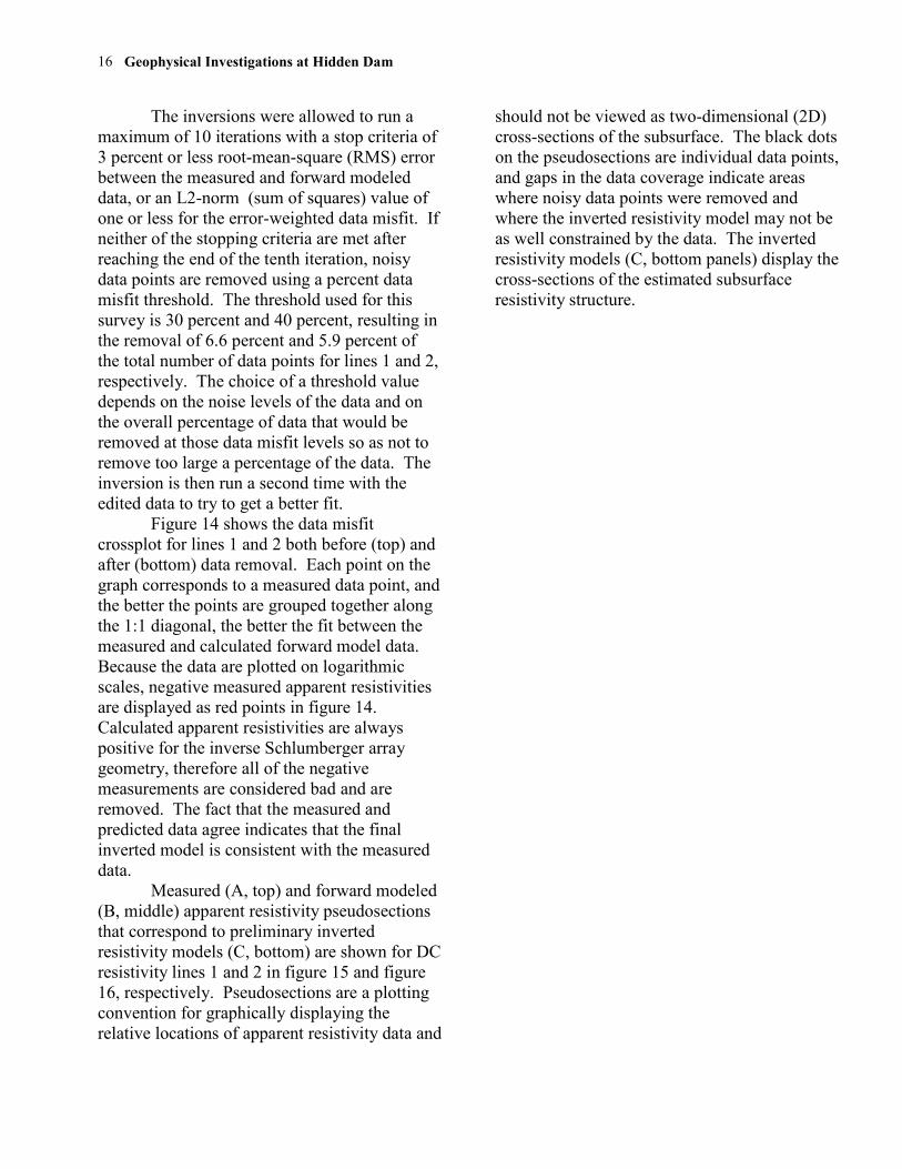
The inversions were allowed to run a maximum of 10 iterations with a stop criteria of 3 percent or less root-mean-square (RMS) error between the measured and forward modeled data, or an L2-norm (sum of squares) value of one or less for the error-weighted data misfit. If neither of the stopping criteria are met after reaching the end of the tenth iteration, noisy data points are removed using a percent data misfit threshold. The threshold used for this survey is 30 percent and 40 percent, resulting in the removal of 6.6 percent and 5.9 percent of the total number of data points for lines 1 and 2, respectively. The choice of a threshold value depends on the noise levels of the data and on the overall percentage of data that would be removed at those data misfit levels so as not to remove too large a percentage of the data. The inversion is then run a second time with the edited data to try to get a better fit.

Figure 14 shows the data misfit crossplot for lines 1 and 2 both before (top) and after (bottom) data removal. Each point on the graph corresponds to a measured data point, and the better the points are grouped together along the 1:1 diagonal, the better the fit between the measured and calculated forward model data. Because the data are plotted on logarithmic scales, negative measured apparent resistivities are displayed as red points in figure 14. Calculated apparent resistivities are always positive for the inverse Schlumberger array geometry, therefore all of the negative measurements are considered bad and are removed. The fact that the measured and predicted data agree indicates that the final inverted model is consistent with the measured data.

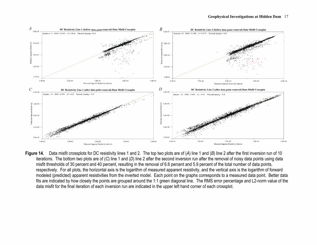
Measured (A, top) and forward modeled (B, middle) apparent resistivity pseudosections that correspond to preliminary inverted resistivity models (C, bottom) are shown for DC resistivity lines 1 and 2 in figure 15 and figure 16, respectively. Pseudosections are a plotting convention for graphically displaying the relative locations of apparent resistivity data and

should not be viewed as two-dimensional (2D) cross-sections of the subsurface. The black dots on the pseudosections are individual data points, and gaps in the data coverage indicate areas where noisy data points were removed and where the inverted resistivity model may not be as well constrained by the data. The inverted resistivity models (C, bottom panels) display the cross-sections of the estimated subsurface resistivity structure.


17

Figure 14. Data misfit crossplots for DC resistivity lines 1 and 2. The top two plots are of (A) line 1 and (B) line 2 after the first inversion run of 10 iterations. The bottom two plots are of (C) line 1 and (D) line 2 after the second inversion run after the removal of noisy data points using data misfit thresholds of 30 percent and 40 percent, resulting in the removal of 6.6 percent and 5.9 percent of the total number of data points, respectively. For all plots, the horizontal axis is the logarithm of measured apparent resistivity, and the vertical axis is the logarithm of forward modeled (predicted) apparent resistivities from the inverted model. Each point on the graphs corresponds to a measured data point. Better data fits are indicated by how closely the points are grouped around the 1:1 green diagonal line. The RMS error percentage and L2-norm value of the data misfit for the final iteration of each inversion run are indicated in the upper left hand corner of each crossplot.


18

Figure 15. DC resistivity line 1 (A) measured data apparent resistivity pseudosection, (B) forward modeled apparent resistivity pseudosection, and (C) inverted resistivity section. The vertical axis on the top two pseudosections is an estimated depth (in feet) of the measured data points, while the vertical axis on the inverted section denotes actual NAVD88 elevation. The horizontal axis for all three images is the downline distance in feet. The black dots on the top two pseudosections represent individual data points, and gaps in the data coverage indicate areas where noisy data points were removed using the percent data misfit threshold removal tool to improve the inverted model fit.


19

Figure 16. DC resistivity line 2 (A) measured data apparent resistivity pseudosection, (B) forward modeled apparent resistivity pseudosection, and (C) inverted resistivity section. The vertical axis on the top two pseudosections is an estimated depth (in feet) of the measured data points, while the vertical axis on the inverted section denotes actual NAVD88 elevation. The horizontal axis for all three images is the downline distance in feet. The black dots on the top two pseudosections represent individual data points, and gaps in the data coverage indicate areas where noisy data points were removed using the percent data misfit threshold removal tool to improve the inverted model fit.


20

Figure 17 shows the inverted sections for lines 1 and 2 at the same scale. In general for both lines, there is a moderately resistive (about 10 to 400 ohm-m; blue to yellow) upper layer that varies in thickness from 0 to approximately 80 ft overlying a strongly resistive (greater than 800 ohm-m; orange to red) layer. Based on the known geology of the area, the upper layer is interpreted to be a combination of alluvial overburden and decomposed, or weathered, granitic bedrock. Without additional borehole or lithologic information to compare directly with the data, it is difficult to conclusively determine the overburden/decomposed bedrock contact. Under saturated conditions, both of these units can have similar electrical properties. The deeper resistor is interpreted as less weathered granitic bedrock, where the more highly weathered/jointed sections have a lower resistivity than the more competent bedrock. These weathered sections in the competent bedrock represent potential groundwater pathways. Several other notable features annotated in figure 17 are described below: • Location E: The most notable feature that is present in both lines is a less resistive zone with a maximum width of about 400 ft interpreted as an alluvial valley between bedrock highs. Based on the trend between lines 1 and 2, the valley appears to trend northeast-southwest and becomes shallower and narrower on line 2. The shallow dark blue zones on line 2 possibly indicate saturated areas of greater porosity or increased concentrations of clay. The source of the thin, shallow discontinuous resistor about 30ft below the surface on both lines is unknown. Although it is possible that it represents a low porosity/permeability layer, this requires further analysis to determine the robustness and structure of this feature in the model. An additional, similar resistor is located between 1,880 and 2,000 ft downline distance on line 2.

• Locations F: There are several highly resistive vertical features that begin about 30 ft below the surface. They tend to have a character indicative of three-dimensional objects either along line or offline improperly imaged with a two-dimensional profile. These objects may represent competent granitic highs, but their true three-dimensional geometry may not be well-resolved. • Locations G: The high near-surface resistivity observed towards the southeastern end of both lines, however, corresponds with several large granite outcrops observed in the field. Somewhat surprisingly, there are only a few areas where the strong resistor reaches the surface, despite the numerous outcrops observed along both lines. The numerous topographically high areas were originally thought to be more resistive outcrops below the surface. The inversions, however, indicate that most of these areas are of only moderate resistivity, and although they may still be granitic, are most likely decomposed and potentially have clay-filled joints and fractures

The large, low-resistivity valley observed at locations E in figure 17 indicates a likely pathway for increased groundwater seepage flow underneath the dam. This conclusion is supported by the fact that this location also corresponds very well with the self-potential anomaly at location A in figure 7 that indicates upward seepage flow in this location. In general, it is likely that the geometry of the more competent (more resistive) bedrock is a strong controlling factor for subsurface flow paths. Regions of thicker alluvium and(or) weathered granite will be preferential pathways for flow. This subsurface structural geometry, in conjunction with the surface topography, is likely the largest factor contributing to the observed seepage at Hidden Dam.


21

Figure 17. Inverted sections for DC resistivity (A) line 1 and (B) line 2. Location E, observed on both lines, is interpreted to be a deep alluvial valley between bedrock highs; locations F are highly resistive features that may represent competent granitic highs with complex geometry; and locations G illustrate high near-surface resistivity associated with large granite outcrops.


22

Future Work Historical measurements of depth to

water in 16 piezometers and 51 observation wells situated on and around Hidden Dam, as well as daily records of reservoir pool elevation, have been obtained for further seepage evaluations at the site. This additional work will involve a time-series analysis of the reservoir elevation and observation well datasets, as well as the development of a 2D finite element model of variably saturated flow in the vicinity of Hidden Dam. Parameters for the flow model will be estimated from existing literature, as well as information gained from the observation wells, piezometers, and geophysical data discussed in this report.

Measurement intervals vary between the piezometer and observation well data sets, as well as among the individual piezometer and well entities included in those data sets. The piezometer data set consists of measurements collected approximately every one to three months between February, 1976, and January, 2007, with more consistent monthly measurements in the latter half of the historical record. Weirs 1 through 6 have also been measured approximately on a monthly basis between June, 1978, and January, 2007, Additionally, daily records of reservoir pool elevation and precipitation exist between February, 1976, and the present.

A two-dimensional numerical model of variably saturated flow through Hidden Dam and beneath the dam foundation will be constructed using the COMSOL 3.5a software. Approximate geometries and material properties representing typical cross sections of the left and right abutments as well as for the closure valley fill will be implemented using schematics and data available in the Hidden Dam foundation report and seepage study (Cedergren, 1980a; U.S. Army Corps of Engineers, 1977). Depth-to-water measurements from both piezometer and observation well data sets will be summarized

in terms of their mean monthly values and used to establish boundary and initial conditions for a numerical model. Grain size curves will be used to estimate additional model input parameters such as residual moisture content, van Genuchten parameters (Van Genuchten, 1980) needed to define soil wetting curves in the partially saturated flow model, and saturated hydraulic conductivities for individual structural elements of Hidden Dam. The relative effect of the downstream toe drainage fill on the distribution of seepage will be evaluated by varying its lateral extent through the core of the modeled dam geometry. Both steady state and transient simulations will be performed.

Figure 18 illustrates a generic example of the type of results that can be obtained from the COMSOL groundwater model. Red colors represent fully-saturated areas, whereas blue is only partially saturated. Contours show lines of equal hydraulic head, and arrows show groundwater flow directions and the relative magnitude of the flow velocity. The simulation uses a reservoir elevation of 510 ft for illustration. Future analyses will also incorporate the true downstream topography, constraints based on the geophysical, observation well, and piezometer data, and will investigate the effect of varying reservoir elevations and dam hydraulic properties.

Conclusions Self-potential and electrical resistivity

surveys at Hidden Dam have provided valuable information regarding the hydrogeologic factors contributing to seepage observed at the site. The self-potential data confirm known seepage areas in the vicinity of the drainage blanket on the right side of the dam, little-to-no seepage on the left side of the dam, and a potentially focused area of seepage immediately above the outlet works. The resistivity cross-sections provide a useful means for delineating subsurface structural variability that controls flow patterns. Enhanced flow is most likely to occur in the regions that contain sediments or


23

Figure 18. Example of a partially saturated groundwater flow model using geometries and estimated hydraulic properties taken from the foundation report (U.S. Army Corps of Engineers, 1977). Solid red colors represent fully-saturated areas, whereas solid blue areas are only partially saturated. Contours show lines of equal hydraulic head, and arrows show groundwater flow directions and relative magnitude. The simulation uses a reservoir elevation of 510 ft for illustrative purposes

weathered granite, and therefore increased porosity and permeability, rather than areas of more competent bedrock. Most prominently, the resistivity models indicate a fairly wide sediment channel that is likely a contributing factor to the known seepage area on the right side of the dam.

With the exception of the area immediately above the outlet works delineated by the self-potential data, it is important to note that the seepage discussed in this study is primarily related to flow underneath (rather than through) the dam structure. The upstream reservoir head, geometry of the competent granite in the subsurface, and downstream surface topography are likely the most significant controlling factors for the observed seepage. This hypothesis will be further

investigated through the use of flow models that can be constrained by the geophysical and observation well data. While it is possible that seepage may also occur through the dam structure, this is not identified in the present survey for two reasons: (1) the inability to record data on the downstream face due to the rip-rap and (2) the fact that seepage through the dam may not occur until the reservoir level is higher.

Acknowledgments This work was carried out with the

support of the U.S. Army Corps of Engineers, Sacramento District, under the supervision of Lewis Hunter. We are grateful for field assistance provided by Jonah Sullivan and Katie


24

Jeffcoat. Significant logistical support and on-site information was provided by the Hidden Dam staff, particularly Phil Smith and Dale Dawson. We thank David Smith, Lewis Hunter, and Kevin Hazleton for their reviews of this manuscript.

References Cited AGI, 2008, Instruction manual for

EarthImager2D version 2.3.0 - resistivity and IP inversion software: Advanced Geosciences, Inc., Austin, TX.

Binley, A., and Kemna, A., 2005, DC resistivity and induced polarization methods, in Rubin, Y., and Hubbard, S.S., eds., Hydrogeophysics: Netherlands, Springer, p. 129-156.

Butler, D.K., 2005, Near-Surface Geophysics: Investigations in Geophysics No. 13: Tulsa, OK, Society of Exploration Geophysicists, 732 p.

Cedergren, H.R., 1980a, Seepage study of Hidden Dam, Fresno River, California: prepared for Department of the Army, Sacramento District, Corps of Engineers.

1980b, Seepage study of Hidden Dam, Fresno River, California: Analysis of data from observation wells put in right abutment seepage areas in 1980: prepared for Department of the Army, Sacramento District, Corps of Engineers.

Corwin, R.F., 1990, The self-potential method for environmental and engineering applications, in Ward, S.H., ed., Geotechnical and Environmental Geophysics: Tulsa, Society of Exploration Geophysicists, p. 127-146.

2005, Investigation of geophysical methods for assessing seepage and internal erosion in embankment dams: Self-potential field data acquisition manual: Canadian Electricity Association Technologies Inc. (CEATI) Report T992700-0205B/1.

2007, Investigation of geophysical methods for assessing seepage and internal erosion in embankment dams: Interpretation of self-

potential data for dam seepage investigations: Canadian Electricity Association Technologies Inc. (CEATI) Report T992700-0205B/3.

Dahlin, T., Sjödahl, P., and Johansson, S., 2008, Investigation of Geophysical Methods for Assessing Seepage and Internal Erosion in Embankment Dams: A Guide to Resistivity Investigation and Monitoring of Embankment Dams: Canadian Electricity Association Technologies Inc. (CEATI).

Ishido, T., and Mizutani, H., 1981, Experimental and Theoretical Basis of Electrokinetic Phenomena in Rock-Water Systems and Its Applications to Geophysics: Journal of Geophysical Research, v. 86, no. NB3, p. 1763-1775.

Loke, M.H., and Barker, R.D., 1996, Rapid least-squares inversion of apparent resistivity pseudosections by a quasi-Newton method: Geophysical Prospecting, v. 44, no. 1, p. 131-152.

Minsley, B.J., Coles, D.A., Vichabian, Y., and Morgan, F.D., 2008, Minimization of self-potential survey mis-ties acquired with multiple reference locations: Geophysics, v. 73, no. 2, p. F71-F81.

Morgan, F.D., Williams, E.R., and Madden, T.R., 1989, Streaming Potential Properties of Westerly Granite with Applications: Journal of Geophysical Research-Solid Earth and Planets, v. 94, no. B9, p. 12449-12461.

Oldenburg, D.W., and Li, Y., 1994, Inversion of induced polarization data: Geophysics, v. 59, no. 9, p. 1327-1341.

Petiau, G., 2000, Second generation of lead-lead chloride electrodes for geophysical applications: Pure and Applied Geophysics, v. 157, no. 3, p. 357-382.

Reynolds, J.M., 1997, An introduction to applied and environmental geophysics: Chichester, England, John Wiley & Sons, 796 p.

Sharma, P.V., 1997, Environmental and engineering geophysics: Cambridge, United


25

Kingdom, Cambridge University Press, 475 p.

Sill, W.R., 1983, Self-Potential Modeling from Primary Flows: Geophysics, v. 48, no. 1, p. 76-86.

Telford, W.M., Geldart, L.P., and Sheriff, R.E., 1990, Applied Geophysics (2nd ed.): Cambridge [England] ; New York, Cambridge University Press, 770 p. p.

U.S. Army Corps of Engineers, 1977, Foundation Report: Hidden Dam Project,

Hensley Lake, Fresno River, California, Madera County: USACE, Sacramento District.

Van Genuchten, M.T., 1980, A Closed-form Equation for Predicting the Hydraulic Conductivity of Unsaturated Soils: Soil Science Society of America Journal, v. 44.

Zhang, J., Mackie, R.L., and Madden, T.R., 1995, 3-D Resistivity Forward Modeling and Inversion Using Conjugate Gradients: Geophysics, v. 60, no. 5, p. 1313-1325.

Documents

USGS OF10-1013