\• I ~ Nat 3: T 4 132

(

vv ~ I -· . ~

~ . ~ ' USING A -BiOTIC INE)EX TO- EVALUATE

WATER QUA~ITY IN-STREAMS

Technical Bulletin No. 132 DEPARTMENT OF NATURAL RESOURCES

Madison, Wisconsin 1982

ts tfl

y

USING A BIOTIC INDEX TO EVALUATE WATER QUALITY IN STREAMS

By William L. Hilsenhoff

Technical Bulletin No. 132 DEPARTMENT OF NATURAL RESOURCES Box 7921, Madison, Wl53707 1982

CONTENTS

2 INTRODUCTION

2 DEVELOPMENT OF THE BIOTIC INDEX

3 EVALUATION OF COLLECTION PROCEDURE

3 Time Required for Collecting, Sorting, and Identification 4 Laboratory Picking vs. Field Picking of Samples 6 Artificial Substrate Samplers as an Alternative Sampling Procedure 7 Reliability of Samples 8 Problems

9 RECOMMENDED SAMPLING PROCEDURE

9 IDENTIFICATION

9 Key to Nymphs of Perlinella 10 Key to Nymphs of /soper/a 10 Key to Nymphs of Baetis 11 Key to Nymphs of Cloeon 11 Key to Nymphs of Pseudocloeon 11 Key to Nymphs of Ephemere/la 12 Key to Nymphs of Eurylophella 12 Key to Nymphs of Serratella 12 Key to Nymphs of Heptagenia 13 Key to Nymphs of Stenonema 13 Key to Nymphs of Argia 14 Key to Nymphs of Neurocordu/ia 14 Key to Larvae of Brachycentrus 14 Key to Larvae of Micrasema 14 Key to Larvae of Chimarra 14 Key to Larvae of Hydropsyche 16 Key to Larvae of Symphitopsyche 16 Key to Adults of Dubiraphia 17 Key to Adults of Optioservus 17 Key to Known Adults of Stenelmis 17 Key to Larvae of Eusimulium 18 Key to Larvae of Simulium

19 TOLERANCE VALUES

21 RECENT SYNONYMS

21 CALCULATION AND EVALUATION OF BIOTIC INDEX VALUES

23 LITERATURE CITED

2

INTRODUCTION

The biotic index I proposed in 1977 has been widely used in Wisconsin and elsewhere to evaluate the water quality of streams. It has proven to be a valuable tool, but it is not yet perfected and results obtained through its use must be evalu­ated with caution. In the past two years we have used the in­dex to evaluate more than 1,000 streams in Wisconsin and have improved our understanding of its use. We have carried

out studies to determine the efficiency and accuracy of the index, have evaluated alternative sampling techniques, and have made substantial changes in many of the tolerance val­ues. In this bulletin I wish to report on recent improvements in the biotic index, point out problems that need to be consid­ered when evaluating results, and provide keys for identifica­tion of species in certain important insect genera.

DEVELOPMENT OF THE BIOTIC INDEX

Since the primary effect of water pollution is on living or­ganisms, assessment of water quality is principally a biological problem. Biological assessment of water quality has been dis­cussed by Hynes (1960), Cairns and Dickson (1973), and many others, and aquatic macroinvertebrates have proven es­pecially valuable for this purpose (Chandler 1970, Gaulin 1973, Roback 1974). To aid in the interpretation of data, in­dexes have been developed. Diversity indexes have received wide attention (Wilhm 1970, land 1976, Hughes 1978), but are not reliable in most situations (Cook 1976, Hilsenhoff 1977, Murphy 1978) and have not been used extensively by aquatic biologists as a tool for measuring water quality. Chan­dler (1970) proposed a "biotic score", and with modifica­tions by Cook ( 1976) and others it has proven more reliable than diversity indexes for evaluating water quality (Murphy 1978) 0

In Europe and the USSR saprobic systems, which evaluate rates of organic decomposition, have been used extensively to monitor water quality, but their use has not been generally ac­cepted in Great Britain and North America. Sladecek ( 1973) comprehensively reviewed the literature on saprobic systems and their use in measuring water quality. Most proposed sa­probic systems involve extensive analysis at the species level of all organisms from bacteria to insects and fish, and while the results may be precise, such a great expenditure of time is probably not warranted when the only objective is evaluation of water quality.

After a two-year study of 53 Wisconsin streams, I proposed using a biotic index of arthropod populations as a rapid method for evaluating water quality (Hilsenhoff 1977) . This index is similar to the saprobic index of Pantel and Buck (1955) and the biotic index of Chutter (1971), but uses only insects, amphipods, and isopods. Beck (1955), Howmiller and Scott ( 1977) , and Winget and Mangum ( 1979) have also proposed biotic indexes that differ somewhat in their de­tails. I use only insects, amphipods, and isopods in my index because they are generally abundant and easily collected from most streams, their fauna is diverse and not mobile, and most species have life cycles of one year or more.

For the purpose of calculating a biotic index, species are assigned pollution tolerance values of 0 to 5 on the basis of previous field studies (Hilsenhoff 1977) -a 0 value is as­signed to species found only in unaltered streams of very high water quality, and a value of 5 is assigned to species known to

occur in severely polluted or disturbed streams. Intermediate values are assigned to species that occur in streams with inter­mediate degrees of pollution or disturbance. When species cannot be identified, genera are assigned values instead. The biotic index is calculated from the formula

N

where n i is the number of individuals of each species (or ge­nus), a i Is the tolerance value assigned to that species (or genus) , and N is the total number of individuals in the sample. The index is an average of tolerance values, and measures saprobity (rate of organic decomposition) and to some ex­tent trophism, which frequently influences saprobity (Caspers and Karbe 1966) . In Wisconsin, the introduction of organic matter or nutrients into a stream and effects of dams are the major causes of deterioration of water quality. Resulting in­creases in saprobity and trophism are readily detected by the biotic index. Heated discharges, heavy metals, and other toxic substances may also be detected by the index, but their ef­fects on the biotic index have not been evaluated. Bacterial and radioactive pollutants must be detected by other means.

The procedure initially recommended for collecting arthro­pods for evaluation of water quality with the biotic index (Hil­senhoff 1977) is as follows: " Use a D-frame aquatic net to sample riffles by disturbing the substrate above the net and allowing dislodged arthropods to be washed into the net by the current. If riffles are absent, rock or gravel runs or debris may be similarly sampled. Place a sample containing about 100 arthropods in a shallow white pan containing a little water. When collecting the samples it is important to not collect sig­nificantly more than 100 arthropods because in large samples, larger and more easily captured arthropods will be most read­ily removed from the pan, creating a biased sample. Using a curved forceps, remove and preserve in 70% ethanol arthro­pods still clinging to the net and those in the pan until 100 have been obtained. Do not collect arthropods less than 3 mm long, except adult Elmidae, because they are difficult to sam­ple and Identify. If 100 arthropods cannot be found in 30 min­utes, those collected within that t ime period would constitute a sample."

2

INTRODUCTION

The biotic index I proposed in 1977 has been widely used in Wisconsin and elsewhere to evaluate the water quality of streams. It has proven to be a valuable tool, but it is not yet perfected and results obtained through its use must be evalu­ated with caution. In the past two years we have used the in­dex to evaluate more than 1,000 streams in Wisconsin and have improved our understanding of its use. We have carried

out studies to determine the efficiency and accuracy of the index, have evaluated alternative sampling techniques, and have made substantial changes in many of the tolerance val­ues. In this bulletin I wish to report on recent improvements in the biotic index, point out problems that need to be consid­ered when evaluating results, and provide keys for identifica­tion of species in certain important insect genera.

DEVELOPMENT OF THE BIOTIC INDEX

Since the primary effect of water pollution is on living or­ganisms, assessment of water quality is principally a biological problem. Biological assessment of water quality has been dis­cussed by Hynes (1960), Cairns and Dickson (1973), and many others, and aquatic macroinvertebrates have proven es­pecially valuable for this purpose (Chandler 1970, Gaulin 1973, Roback 1974). To aid in the interpretation of data, in­dexes have been developed. Diversity indexes have received wide attention (Wilhm 1970, land 1976, Hughes 1978), but are not reliable in most situations (Cook 1976, Hilsenhoff 1977, Murphy 1978) and have not been used extensively by aquatic biologists as a tool for measuring water quality. Chan­dler (1970) proposed a "biotic score", and with modifica­tions by Cook ( 1976) and others it has proven more reliable than diversity indexes for evaluating water quality (Murphy 1978) 0

In Europe and the USSR saprobic systems, which evaluate rates of organic decomposition, have been used extensively to monitor water quality, but their use has not been generally ac­cepted in Great Britain and North America. Sladecek ( 1973) comprehensively reviewed the literature on saprobic systems and their use in measuring water quality. Most proposed sa­probic systems involve extensive analysis at the species level of all organisms from bacteria to insects and fish, and while the results may be precise, such a great expenditure of time is probably not warranted when the only objective is evaluation of water quality.

After a two-year study of 53 Wisconsin streams, I proposed using a biotic index of arthropod populations as a rapid method for evaluating water quality (Hilsenhoff 1977) . This index is similar to the saprobic index of Pantel and Buck (1955) and the biotic index of Chutter (1971), but uses only insects, amphipods, and isopods. Beck (1955), Howmiller and Scott ( 1977) , and Winget and Mangum ( 1979) have also proposed biotic indexes that differ somewhat in their de­tails. I use only insects, amphipods, and isopods in my index because they are generally abundant and easily collected from most streams, their fauna is diverse and not mobile, and most species have life cycles of one year or more.

For the purpose of calculating a biotic index, species are assigned pollution tolerance values of 0 to 5 on the basis of previous field studies (Hilsenhoff 1977) -a 0 value is as­signed to species found only in unaltered streams of very high water quality, and a value of 5 is assigned to species known to

occur in severely polluted or disturbed streams. Intermediate values are assigned to species that occur in streams with inter­mediate degrees of pollution or disturbance. When species cannot be identified, genera are assigned values instead. The biotic index is calculated from the formula

N

where n i is the number of individuals of each species (or ge­nus), a i Is the tolerance value assigned to that species (or genus) , and N is the total number of individuals in the sample. The index is an average of tolerance values, and measures saprobity (rate of organic decomposition) and to some ex­tent trophism, which frequently influences saprobity (Caspers and Karbe 1966) . In Wisconsin, the introduction of organic matter or nutrients into a stream and effects of dams are the major causes of deterioration of water quality. Resulting in­creases in saprobity and trophism are readily detected by the biotic index. Heated discharges, heavy metals, and other toxic substances may also be detected by the index, but their ef­fects on the biotic index have not been evaluated. Bacterial and radioactive pollutants must be detected by other means.

The procedure initially recommended for collecting arthro­pods for evaluation of water quality with the biotic index (Hil­senhoff 1977) is as follows: " Use a D-frame aquatic net to sample riffles by disturbing the substrate above the net and allowing dislodged arthropods to be washed into the net by the current. If riffles are absent, rock or gravel runs or debris may be similarly sampled. Place a sample containing about 100 arthropods in a shallow white pan containing a little water. When collecting the samples it is important to not collect sig­nificantly more than 100 arthropods because in large samples, larger and more easily captured arthropods will be most read­ily removed from the pan, creating a biased sample. Using a curved forceps, remove and preserve in 70% ethanol arthro­pods still clinging to the net and those in the pan until 100 have been obtained. Do not collect arthropods less than 3 mm long, except adult Elmidae, because they are difficult to sam­ple and Identify. If 100 arthropods cannot be found in 30 min­utes, those collected within that t ime period would constitute a sample."

EVALUATION OF COLLECTION PROCEDURE

Beginning in 1977 several studies were carried out to deter­mine the efficiency and reliability of this procedure, the impor­tance of species identification, and the relative merits of alter­native sampling and sorting procedures. The results of these studies are reported below.

TIME REQUIRED FOR COLLECTING, SORTING, AND IDENTIFICATION

To learn exactly how long it takes to evaluate the water quality of a stream using the recommended procedure, and to determine if precision gained by species identifications war­rants the additional expenditure of time, a study of 53 Wiscon­sin streams was initiated in 1977. These were the same 53 streams previously studied (Hilsenhoff 1977), and were se­lected because they encompassed a wide range of sizes, cur­rents, substrates, water chemistries, and water quality.

Materials and Methods

Sampling was initiated May 20 and completed June 8, with streams farthest south being sampled first. A sample was collected from each stream according to procedures already described. Hemiptera and adults of Dytiscidae, Gyrinidae, Haliplidae, and Hydrophilidae were not collected because they do not rely on the stream for oxygen. If 100 arthropods were not obtained in the first sample, an additional sample was collected. If 100 arthropods were not collected in one-half hour, the number collected in that time period was used as the sample.

In the laboratory, samples from the 53 streams were di­vided at random into two groups. I sorted the arthropods In 26 samples into 1-dram vials, identified them to genus, and la­beled the vials. The remaining 27 samples were similarly sorted and labeled by a student with no entomological training and only one week of experience in sorting such samples, but she did not attempt identification. I later identified these speci­mens to genus and corrected errors in sorting. Numbers in each genus were recorded and a biotic index was calculated for each stream using published values (Hilsenhoff 1977) and values for genera based on weighted averages of species val­ues. I then identified to species insects in the genera listed in Table 1 and calculated a biotic index using tolerance values for these species. The time needed for each laboratory proce­dure was recorded, as was the time elapsed from arrival of the vehicle at each stream until its departure.

Except for the Arkansaw River and Wisconsin River #4, the 53 stream sites sampled in 1977 were sampled again in 1978 at the same time of the year, some in conjunction with another experiment which is reported below. Hydropsyche and some Symphltopsyche were identified to species in both the 1977 and 1978 samples, and species biotic index values were cal­culated for each year using new tolerance values published in this bulletin. Generic biotic index values were also calculated using weighted tolerance values as follows: Baetis 2, Ephemerella 1, Eurylophel/a 1, Serra tel/a 1, Heptagenia 2, Stenonema 2, Brachycentrus 1, Hydropsyche 3, Symphitopsyche 2, Chimerrq 2 , Dubiraphia 3, Opti­oservus 2, Stenelmis 3, Eusimulium 2, and Simulium 3.

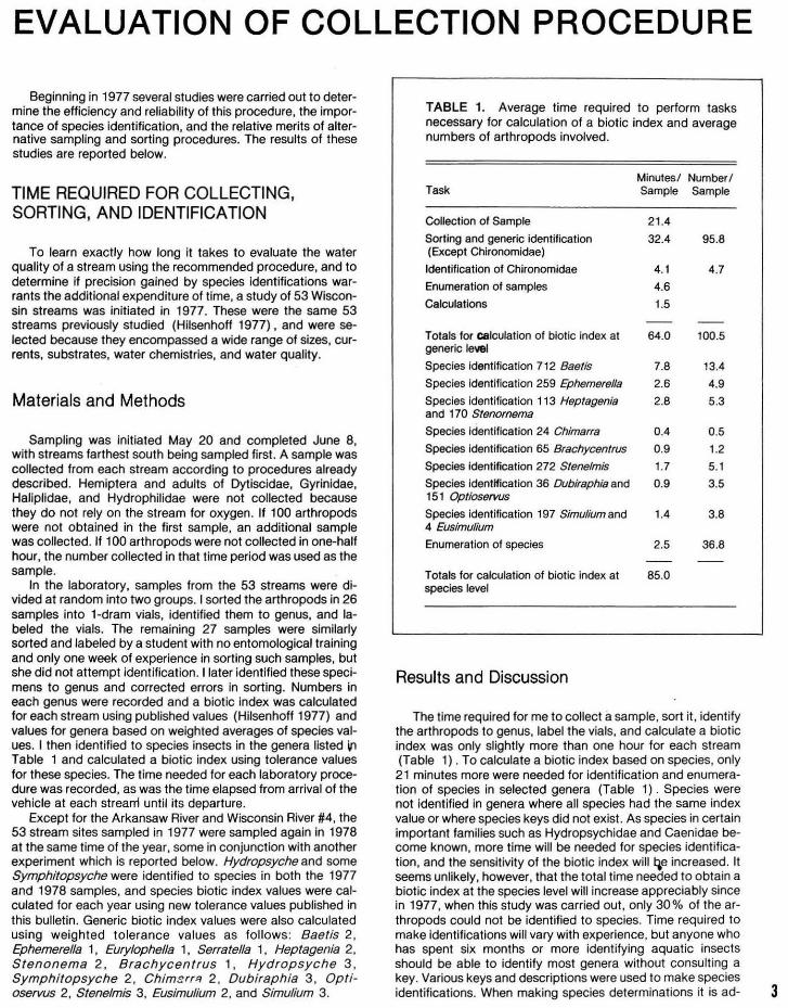
TABLE 1. Average time required to perform tasks necessary for calculation of a biotic index and average numbers of arthropods involved.

Minutes/ Number/ Task Sample Sample

Collection of Sample 21.4

Sorting and generic identification 32.4 95.8 (Except Chironomidae)

Identification of Chironomidae 4.1 4.7

Enumeration of samples 4.6

Calculations 1.5

Totals for calculation of biotic index at 64.0 100.5 generic level

Species identification 712 Baetis 7.8 13.4

Species identification 259 £phemerella 2.6 4.9

Species identification 113 Heptagenia 2.8 5.3 and 170 Stenornema

Species identification 24 Chimarra 0.4 0.5

Species identification 65 Brachycentrus 0.9 1.2

Species identification 272 Stenelmis 1.7 5.1

Species identification 36 Dubiraphia and 0.9 3.5 151 Optioservus

Species identification 197 Simulium and 1.4 3.8 4 Eusimulium

Enumeration of species 2.5 36.8

Totals for calculation of biotic index at 85.0 species level

Results and Discussion

The time required for me to collect a sample, sort it, identify the arthropods to genus, label the vials, and calculate a biotic index was only slightly more than one hour for each stream (Table 1) . To calculate a biotic index based on species, only 21 minutes more were needed for identification and enumera­tion of species in selected genera (Table 1). Species were not identified in genera where all species had the same index value or where species keys did not exist . As species in certain important families such as Hydropsychidae and Caenidae be­come known, more time will be needed for species identifica­tion, and the sensitivity of the biotic index will ~e increased. It seems unlikely, however, that the total time needed to obtain a biotic index at the species level will increase appreciably since in 1977, when this study was carried out, only 30% of the ar­thropods could not be identified to species. Time required to make identifications will vary with experience, but anyone who has spent six months or more identifying aquatic insects should be able to identify most genera without consult ing a key. Various keys and descriptions were used to make species identifications. When making species determinations it is ad- 3

4

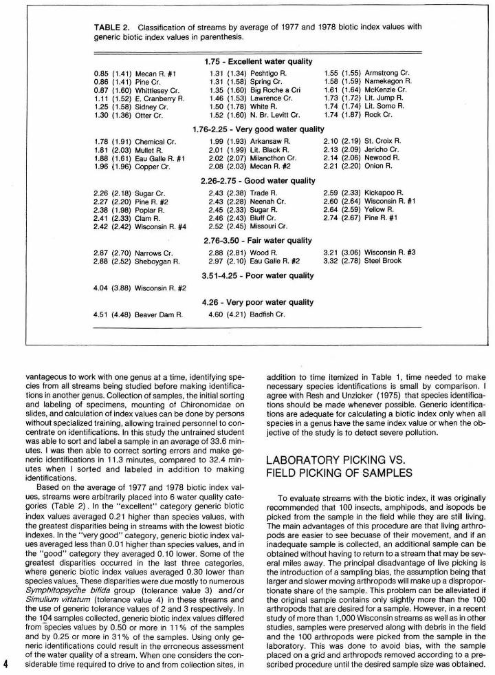
TABLE 2. Classification of streams by average of 1977 and 1978 biotic index values with generic biotic index values in parenthesis.

0.85 (1 .41) Mecan R. #1 0.86 (1.41) Pine Cr.

1.75- Excellent water quality

1.31 (1 .34) Peshtigo R. 1.55 (1.55) Armstrong Cr. 1.58 ( 1.59) Namekagon R. 1.61 (1.64) McKenzie Cr. 1.73 (1.72) Lit. Jump R. 1.74 (1 .74) Lit. Somo R. 1.74 (1 .87) Rock Cr.

1.31 ( 1.58) Spring Cr. 0.87 ( 1.60) Whittlesey Cr. 1.1 1 ( 1.52) E. Cranberry R. 1.25 ( 1.58) Sidney Cr.

1.35 ( 1.60) Big Roche a Crl 1.46 (1 .53) Lawrence Cr. 1.50 ( 1.78) White R.

1.30 (1.36) Otter Cr. 1.52 ( 1.60) N. Br. Levitt Cr.

1. 76-2.25 - Very good water quality

1.78 (1 .91) Chemical Cr. 1.81 (2.03) Mullet R. 1.88 (1.61) Eau GalleR. #1 1.96 (1.96) Copper Cr.

1.99 (1.93) Arkansaw R. 2.01 (1.99) Lit. Black R. 2.02 (2.07) Milancthon Cr. 2.08 (2.03) Mecan R. #2

2.10 (2.19) St. Croix R. 2.13 (2.09) Jericho Cr. 2.14 (2.06) Newood R. 2.21 (2.20) Onion R.

2.26 (2.18) Sugar Cr. 2.27 (2.20) Pine R. #2 2.38 (1 .98) Poplar R. 2.41 (2.33) Clam R.

2.26-2.75- Good water quality

2.43 (2.38) Trade R. 2.59 (2.33) Kickapoo R. 2.60 (2.64) Wisconsin R. #1 2.64 (2.59) Yellow R.

2.43 (2.28) Neenah Cr. 2.45 (2.33) Sugar R. 2.46 (2.43) Bluff Cr. 2.74 (2.67) PineR. #1

2.42 (2.42) Wisconsin R. #4 2.52 (2.45) Missouri Cr.

2.87 (2.70) Narrows Cr. 2.88 (2.52) Sheboygan R.

2. 76-3.50 - Fair water quality

2.88 (2.81) Wood R. 3.21 (3.06) Wisconsin R. #3 3.32 (2. 78) Steel Brook 2.97 (2.10) Eau GalleR. #2

3.51-4.25 - Poor water quality

4.04 (3.88) Wisconsin R. #2

4.51 (4.48) Beaver Dam R.

4.26 - Very poor water quality

4.60 (4.21) Badfish Cr.

vantageous to work with one genus at a time. identifying spe­cies from all streams being studied before making identifica­tions in another genus. Collection of samples. the initial sorting and labeling of specimens, mounting of Chironomidae on slides, and calculation of index values can be done by persons without specialized training, allowing trained personnel to con­centrate on identifications. In this study the untrained student was able to sort and label a sample in an average of 33.6 min­utes. I was then able to correct sorting errors and make ge­neric identifications in 11.3 minutes, compared to 32.4 min­utes when I sorted and labeled in addition to making identifications.

Based on the average of 1977 and 1978 biotic index val­ues, streams were arbitrarily placed into 6 water quality cate­gories (Table 2). In the "excellent" category generic biotic index values averaged 0.21 higher than species values, with the greatest disparities being in streams with the lowest biotic indexes. In the "very good" category, generic biotic index val­ues averaged less than 0.01 higher than species values, and in the " good" category they averaged 0.10 lower. Some of the greatest disparities occurred in the last three categories. where generic biotic index values averaged 0.30 lower than species values. These disparities were due mostly to numerous Symphitopsyche bifida group (tolerance value 3) and/or Simulium vittatum (tolerance value 4) in these streams and the use of generic tolerance values of 2 and 3 respectively. In the 104 samples collected, generic biotic index values differed from species values by 0.50 or more in 11 % of the samples and by 0.25 or more in 31% of the samples. Using only ge­neric identifications could result in the erroneous assessment of the water quality of a stream. When one considers the con­siderable time required to drive to and from collection sites, in

addition to time itemized in Table 1, time needed to make necessary species identifications is small by comparison. I agree with Resh and Unzicker (1975) that species identifica­tions should be made whenever possible. Generic identifica­tions are adequate for calculating a biotic index only when· all species in a genus have the same index value or when the ob­jective of the study is to detect severe pollution.

LABORATORY PICKING VS. FIELD PICKING OF SAMPLES

To evaluate streams with the biotic index, it was originally recommended that 100 insects, amphipods, and isopods be picked from the sample in the field while they are still living. The main advantages of this procedure are that living arthro­pods are easier to see becuase of their movement, and if an inadequate sample is collected, an additional sample can be obtained without having to return to a stream that may be sev­eral miles away. The principal disadvantage of live picking is the introduction of a sampling bias, the assumption being that larger and slower moving arthropods will make up a dispropor­tionate share of the sample. This problem can be alleviated if the original sample contains only slightly more than the 100 arthropods that are desired for a sample. However, in a recent study of more than 1,000 Wisconsin streams as well as in other studies, samples were preserved along with debris in the field and the 100 arthropods were picked from the sample in the laboratory. This was done to avoid bias, with the sample placed on a grid and arthropods removed according to a pre­scribed procedure until the desired sample size was obtained.

A study was carried out to determine how the two methods of picking affect biotic index values.

Materials and Methods

Six samples of 100 arthropods were collected from each of 5 Wisconsin streams in late June 1981 to determine if bias is present in the two sampling procedures and to estimate the efficiency of each procedure. The samples were alternately picked in the field or preserved in alcohol and returned to the laboratory for picking. Because of the scarcity of arthropods, 12 samples of 50 arthropods were collected from Armstrong Creek. The time required to remove arthropods from a sample in the laboratory, sort them into labeled vials, and identify them to genus was recorded so that it could be compared with the t ime needed to sort and identify field-picked samples in a previous experiment (Table 1). Biotic index values were cal­culated for all samples and compared with a t test. Numbers of individuals collected in each of the 17 most prevalent groups of arthropods were tabulated and compared to deter­mine if a sorting bias existed.

Results and Discussion

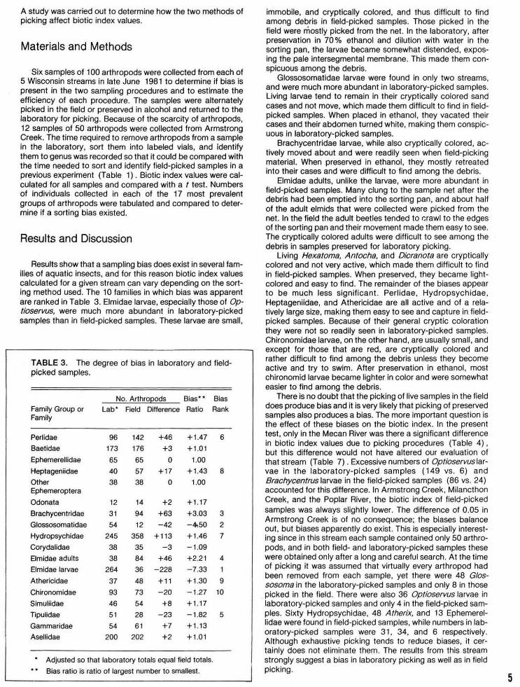
Results show that a sampling bias does exist In several fam­ilies of aquatic insects, and for this reason biotic index values calculated for a given stream can vary depending on the sort­ing method used. The 10 families in which bias was apparent are ranked in Table 3. Elmidae larvae, especially those of Op­tioservus, were much more abundant in laboratory-picked samples than in field-picked samples. These larvae are small,

TABLE 3. The degree of bias in laboratory and field-picked samples.

No. Arthro~ods Bias* • Bias Family Group or Lab* Field Difference Ratio Rank Family

Perlidae 96 142 +46 +1.47 6

Baelidae 173 176 +3 + 1.01

Ephemerellidae 65 65 0 1.00

Heptageniidae 40 57 +17 + 1.43 8

Other 38 38 0 1.00 Ephemeroptera Odonata 12 14 +2 + 1.17

Brachycentridae 31 94 +63 +3.03 3

Glossosomatidae 54 12 - 42 -4..50 2

Hydropsychidae 245 358 +1 13 +1.46 7

Corydalidae 38 35 -3 - 1.09

Elmidae adults 38 84 +46 +2.21 4

Elmidae larvae 264 36 - 228 - 7.33 1

Athericidae 37 48 +11 +1 .30 9

Chironomidae 93 73 -20 -1.27 10

Simuliidae 46 54 +8 +1 .17

Tipulidae 51 28 -23 -1 .82 5

Gammaridae 54 61 +7 +1 .13

Asellidae 200 202 +2 +1 .01

. Adjusted so that laboratory totals equal field totals . Bias ratio is ratio of largest number to smallest.

immobile, and cryptically colored, and thus difficult to find among debris in field-picked samples. Those picked in the field were mostly picked from the net. In the laboratory, after preservation in 70 % ethanol and dilution with water In the sorting pan, the larvae became somewhat distended, expos­ing the pale intersegmental membrane. This made them con­spicuous among the debris.

Glossosomatidae larvae were found in only two streams, and were much more abundant in laboratory-picked samples. living larvae tend to remain in their cryptically colored sand cases and not move, which made them difficult to find in field­picked samples. When placed in ethanol, they vacated their cases and their abdomen turned white, making them conspic­uous in laboratory-picked samples.

Brachycentridae larvae, while also cryptically colored, ac­tively moved about and were readily seen when field-picking material. When preserved in ethanol, they mostly retreated into their cases and were difficult to find among the debris.

Elmidae adults, unlike the larvae, were more abundant in field-picked samples. Many clung to the sample net after the debris had been emptied into the sorting pan, and about half of the adult elmids that were collected were picked from the net. In the field the adult beetles tended to r.rawl to the edges of the sorting pan and their movement made them easy to see. The cryptically colored adults were difficult to see among the debris in samples preserved for laboratory picking.

living Hexatoma, Antocha, and Dicranota are cryptically colored and not very active, which made them difficult to find in field-picked samples. When preserved, they became light­colored and easy to find. The remainder of the biases appear to be much less significant. Perlidae , Hydropsychidae, Heptageniidae, and Athericidae are all active and of a rela­tively large size, making them easy to see and capture in field­picked samples. Because of their general cryptic coloration they were not so readily seen in laboratory-picked samples. Chironomidae larvae, on the other hand, are usually small, and except for those that are red, are cryptically colored and rather difficult to find among the debris unless they become active and try to swim. After preservation in ethanol, most chironomid larvae became lighter in color and were somewhat easier to find among the debris.

There is no doubt that the picking of live samples in the field does produce bias and it is very likely that picking of preserved samples also produces a bias. The more important question is the effect of these biases on the biotic index. In the present test, only in the Mecan River was there a significant difference in biotic index values due to picking procedures (Table 4), but this difference would not have altered our evaluation of that stream (Table 7) . Excessive numbers of Optioservuslar­vae in the laboratory-picked samples ( 149 vs. 6) and Brachycentrus larvae in the field-picked samples (86 vs. 24) accounted for this difference. In Armstrong Creek, Milancthon Creek, and the Poplar River, the biot ic index of field-picked samples was always slightly lower. The difference of 0.05 in Armstrong Creek is of no consequence; the biases balance out, but biases apparently do exist. This is especially interest­ing since in this stream each sample contained only 50 arthro­pods, and in both field- and laboratory-picked samples these were obtained only after a long and careful search. At the time of picking it was assumed that virtually every arthropod had been removed from each sample, yet there were 48 Glos­sosoma in the laboratory-picked samples and only 8 in those

. picked in the field. There were also 36 Optioservus larvae in laboratory-picked samples and only 4 in the field-picked sam­ples. Sixty Hydropsychidae, 48 Atherix, and 13 Ephemerel­lidae were found in field-picked samples, while numbers in lab­oratory-picked samples were 31 , 34, and 6 respectively. Although exhaustive picking tends to reduce biases, it cer­tainly does not eliminate them. The results from this stream strongly suggest a bias in laboratory picking as well as in field picking.

5

6·

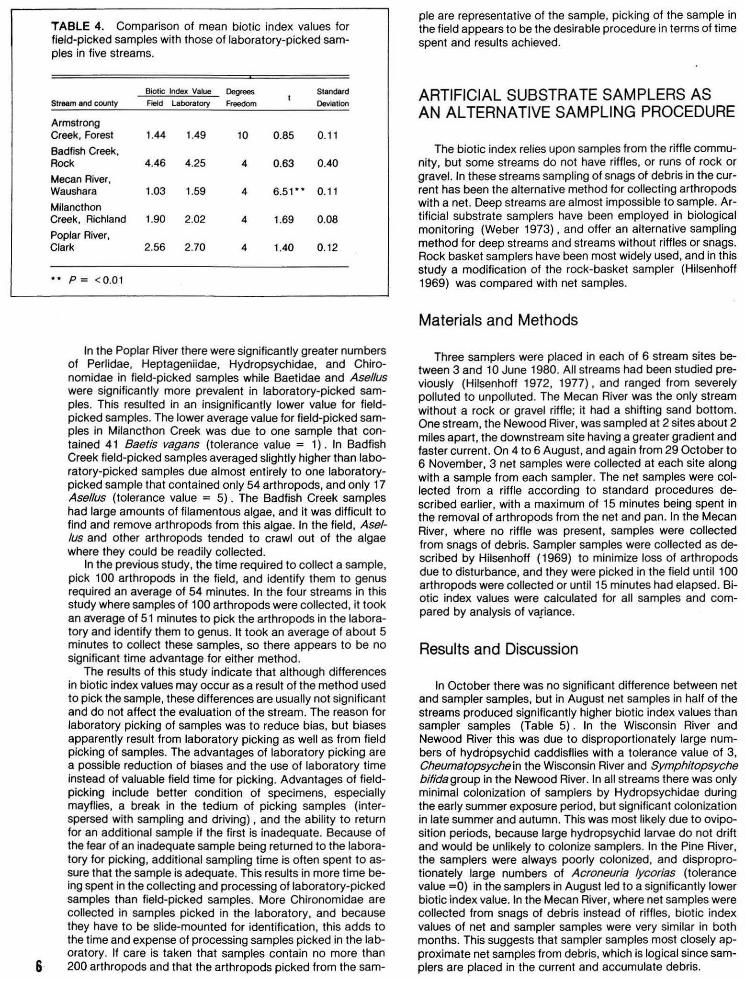
TABLE 4. Comparison of mean biotic index values for field-picked samples with those of laboratory-picked sam­ples in five streams.

Biotic Index Value Degrees Standard

Stream and county Field Laboratory Freedom Deviation

Armstrong Creek, Forest 1.44 1.49 10 0.85 0. 11

Badfish Creek, Rock 4.46 4.25 4 0.63 0.40

Mecan River, Waushara 1.03 1.59 4 6.51** 0.11

Milancthon Creek, Richland 1.90 2.02 4 1.69 0.08 Poplar River, Clark 2.56 2.70 4 1.40 0.12

•• p = < 0.01

In the Poplar River there were significantly greater numbers of Perlidae, Heptageniidae, Hydropsychidae, and Chiro­nomidae in field-picked samples while Baetidae and Asellus were significantly more prevalent in laboratory-picked sam­ples. This resulted in an insignificantly lower value for field­picked samples. The lower average value for field-picked sam­ples in Milancthon Creek was due to one sample that con­tained 41 Baetis vagans (tolerance value = 1) . In Bad fish Creek field-picked samples averaged slightly higher than labo­ratory-picked samples due almost entirely to one laboratory­picked sample that contained only 54 arthropods, and only 17 Asellus (tolerance value = 5). The Badfish Creek samples had large amounts of filamentous algae, and it was difficult to find and remove arthropods from this algae. In the field, Asel­/us and other arthropods tended to crawl out of the algae where they could be readily collected.

In the previous study, the time required to collect a sample, pick 100 arthropods in the field, and identify them to genus required an average of 54 minutes. In the four streams in this study where samples of 100 arthropods were collected, it took an average of 51 minutes to pick the arthropods in the labora­tory and identify them to genus. It took an average of about 5 minutes to collect these samples, so there appears to be no significant time advantage for either method.

The results of this study indicate that although differences in biotic index values may occur as a result of the method used to pick the sample, these differences are usually not significant and do not affect the evaluation of the stream. The reason for laboratory picking of samples was to reduce bias. but biases apparently result from laboratory picking as well as from field picking of samples. The advantages of laboratory picking are a possible reduction of biases and the use of laboratory time instead of valuable field time for picking. Advantages of field­picking include better condition of specimens, especially mayflies, a break in the tedium of picking samples (inter­spersed with sampling and driving) , and the ability to return for an additional sample if the first is inadequate. Because of the fear of an inadequate sample being returned to the labora­tory for picking, additional sampling time is often spent to as­sure that the sample is adequate. This results in more time be­ing spent in the collecting and processing of laboratory-picked samples than field-picked samples. More Chironomidae are collected in samples picked in the laboratory. and because they have to be slide-mounted for identification, this adds to the time and expense of processing samples picked in the lab­oratory. If care is taken that samples contain no more than 200 arthropods and that the arthropods picked from the sam-

pie are representative of the sample, picking of the sample in the field appears to be the desirable procedure in terms of time spent and results achieved.

ARTIFICIAL SUBSTRATE SAMPLERS AS AN ALTERNATIVE SAMPLING PROCEDURE

The biotic index relies upon samples from the riffle commu­nity, but some streams do not have riffles, or runs of rock or gravel. In these streams sampling of snags ot debris in the cur­rent has been the alternative method for collecting arthropods with a net. Deep streams are almost impossible to sample. Ar­tificial substrate samplers have been employed in biological monitoring (Weber 1973), and offer an alternative sampling method for deep streams and streams without riffles or snags. Rock basket samplers have been most widely used, and in this study a modification of the rock-basket sampler (Hilsenhoff 1969) was compared with net samples.

Materials and Methods

Three samplers were placed in each of 6 stream sites be­tween 3 and 10 June 1980. All streams had been studied pre­viously (Hilsenhoff 1972, 1977), and ranged from severely polluted to unpolluted. The Mecan River was the only stream without a rock or gravel riffle; it had a shifting sand bottom. One stream, the Newood River, was sampled at 2 sites about 2 miles apart, the downstream site having a greater gradient and faster current. On 4 to 6 August, and again from 29 October to 6 November, 3 net samples were collected at each site along with a sample from each sampler. The net samples were col­lected from a riffle according to standard procedures de­scribed earlier, with a maximum of 15 minutes being spent in the removal of arthropods from the net and pan. In the Mecan River, where no riffle was present, samples were collected from snags of debris. Sampler samples were collected as de­scribed by Hilsenhoff (1969) to minimize loss of arthropods due to disturbance, and they were picked in the field until 100 arthropods were collected or until 15 minutes had elapsed. Bi­otic index values were calculated for all samples and com­pared by analysis of variance.

Results and Discussion

In October there was no significant difference between net and sampler samples, but in August net samples in half of the streams produced significantly higher biotic index values than sampler samples (Table 5) . In the Wisconsin River and Newood River t his was due to disproportionately large num­bers of hydropsychid caddlsflies with a tolerance value of 3, Cheumatopsyche in the Wisconsin River and Symphitopsyche bifidagroup in the Newood River. In all streams there was only minimal colonization of samplers by Hydropsychidae during the early summer exposure period, but significant colonization in late summer and autumn. This was most likely due to ovipo­sition periods, because large hydropsychid larvae do not drift and would be unlikely to colonize samplers. In the Pine River, the samplers were always poorly colonized, and dispropro­tionately large numbers of Acroneuria lycorias (tolerance value =0) in the samplers in August led to a significantly lower biotic index value. In the Mecan River, where net samples were collected from snags of debris instead of riffles, biotic index values of net and sampler samples were very similar in both months. This suggests that sampler samples most closely ap­proximate net samples from debris, which is logical since sam­plers are placed in the current and accumulate debris.

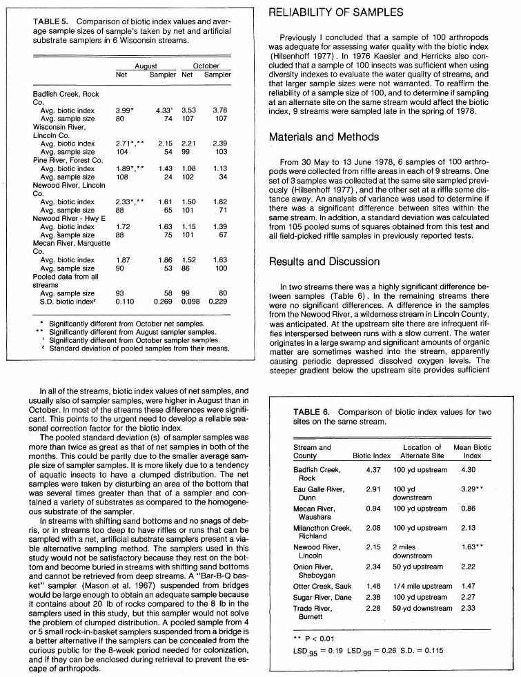
TABLE5. Comparison of biotic index values and aver-age sample sizes of sample's taken by net and artificial substrate samplers in 6 Wisconsin streams.

August October" Net Sampler Net Sampler

Badfish Creek, Rock Co.

Avg. biotic index 3.99* 4.33' 3.53 3.78 Avg. sample size 80 74 107 107

Wisconsin River, Lincoln Co.

Avg. biotic index 2.71*,** 2.15 2.21 2.39 Avg. sample size 104 54 99 103

Pine River, Forest Co. Avg. biotic index 1.89*,** 1.43 1.08 1.13 Avg. sample size 108 24 102 34

Newood River, Lincoln Co.

Avg. biotic index 2.33* ,*. 1.61 1.50 1.82 Avg. sample size 88 65 101 71

Newood River - Hwy E Avg. biotic index 1.72 1.63 1.15 1.39 Avg. Sample size 88 75 101 67

Mecan River, Marquette Co.

Avg. biotic index 1.87 1.86 1.52 1.63 Avg. sample size 90 53 86 100

Pooled data from all streams

Avg. sample size 93 58 99 80 S.D. biotic index• 0.110 0.269 0.098 0.229

* Significantly different from October net samples. Significantly different from August sampler samples.

1 Significantly different from October sampler samples. 2 Standard deviation of pooled samples from their means.

In all of the streams, biotic index values of net samples, and usually also of sampler samples, were higl:ler in August than in October. In most of the streams these differences were signifi­cant. This points to the urgent need to develop a reliable sea­sonal correction factor for the biotic index.

The pooled standard deviation (s) of sampler samples was more than twice as great as that of net samples in both of the months. This could be partly due to the smaller average sam­ple size of sampler samples. It is more likely due to a tendency of aquatic insects to have a clumped distribution . The net samples were taken by disturbing an area of the bottom that was several times greater than that of a sampler and con­tained a variety of substrates as compared to the homogene­ous substrate of the sampler.

In streams with shifting sand bottoms and no snags of deb­ris, or in streams too deep to have riffles or runs that can be sampled with a net, artificial substrate samplers present a via­ble alternative sampling method. The samplers used in this study would not be satisfactory because they rest on the bot­tom and become buried in streams with shifting sand bottoms and cannot be retrieved from deep streams. A "Bar-B-O bas­ket'' sampler (Mason et al. 1967) suspended from bridges would be large enough to obtain an adequate sample because it contains about 20 lb of rocks compared to the 8 lb in the samplers used in this study, but this sampler would not solve the problem of clumped distribution. A pooled sample from 4 or 5 small rock-in-basket samplers suspended from a bridge is a better alternative if the samplers can be concealed from the curious public for the 8-week period needed for colonization, and if they can be enclosed during retrieval to prevent the es­cape of arthropods.

RELIABILITY OF SAMPLES

Previously I concluded that a sample of 100 arthropods was adequate for assessing water quality with the biotic index (Hilsenhoff 1977) . In 1976 Kaesler and Herricks also con­

cluded that a sample of 1 00 insects was sufficient when using diversity indexes to evaluate the water quality of streams, and that larger sample sizes were not warranted. To reaffirm the reliability of a sample size of 100, and to determine if sampling at an alternate site on the same stream would affect the biotic index, 9 streams were sampled late in the spring of 1978.

Materials and Methods

From 30 May to 13 June 1978, 6 samples of 100 arthro­pods were collected from riffle areas in each of 9 streams. One set of 3 samples was collected at the same site sampled previ­ously (Hilsenhoff 1977), and the other set at a riffle some dis­tance away. An analysis of variance was used to determine if there was a significant difference between sites w ithin the same stream. In addition, a standard deviation was calculated from 105 pooled sums of squares obtained from this test and all field-picked riffle samples in previously reported tests.

Results and Discussion

In two streams there was a highly significant difference be­tween samples (Table 6) . In the remaining streams there were no significant differences. A difference in the samples from the Newood River, a wilderness stream in Lincoln County, was anticipated. At the upstream site there are infrequent rif­fles interspersed between runs with a slow current. The water originates in a large swamp and significant amounts of organic matter are sometimes washed into the stream, apparently causing periodic depressed dissolved oxygen levels. The steeper gradient below the upstream site provides sufficient

TABLE 6. Comparison of biotic index values for two sites on the same stream.

Stream and Location of Mean Biotic County Biotic Index Alternate Site Index

Badfish Creek, 4.37 1 00 yd upstream 4.30 Rock

Eau Galle River, 2.91 100 yd 3.29** Dunn downstream

Mecan River, 0.94 100 yd upstream 0.86 Waushara

Milancthon Creek, 2.08 100 yd upstream 2.13 Richland

Newood River, 2.15 2 miles 1.63** Lincoln downstream

Onion River, 2.34 50 yd upstream 2.22 Sheboygan

Otter Creek, Sauk 1.48 1 I 4 mile upstream 1.47

Sugar River, Dane 2.38 100 yd upstream 2.27

Trade River, 2.28 SO·yd downstream 2.33 Burnett

•• p < 0.01

LSD.95 = 0.19 LSD.99 = 0.26 S.D. = 0.115

8

riffles and oxygen to reaerate the stream at the sampling site 2 miles downstream, accounting for a much lower biotic index at that site. The phenomenon of occasionally elevated biotic in­dex values resulting from depressed oxygen levels in wilder­ness streams that originate in swamps was noted previously by Joe Eilers (pers. comm.) . It most frequently occurs after periods of heavy rain and flooding .

A highly significant difference in biotic index was also en­countered in the Eau Galle River in Dunn County, and this was not expected. This sampling site on the Eau Galle River is about 100 yd below a hydroelectric dam, where there is sig­nificant aeration of the water as it passes through turbines or over a high spillway. Effects of decomposition of organic mat­ter produced in the impoundment would be more prominent farther downstream, and would account for a significantly higher biotic index at the downstream site.

The standard deviation from pooled sums of squares in this and all other replicated experiments in which 100 arthropods were collected with a net and picked in the field , was 0.098. This means that 95% of biotic indexes calculated from a sam­ple of 100 arthropods should be within 0.19 of the true index value, and 99% should be within 0.25.

A previous test in which field-picked samples were com­pared with laboratory-picked samples provided the only set of samples with replicates of 50 arthropods instead of 100. There were 6 replicates of 50 in the samples from Armstrong Creek, and the data from these replicates were combi_ned in all possi­ble combinations to produce sample sizes of 100, 150, and 200. Biotic index values were calculated for all sample sizes. In the field-picked samples the standard deviation was com­pared for all sample sizes and it was 0.071 for replicates of 50, and 0.035, 0.031 and 0.026 tor replicates of 100, 150, and 200 respectively. This indicates that a sample size of 50 ar­thropods is only half as reliable as the standard sample of 100, and reaffirms that the additional time needed to collect and process larger samples Is probably not justified because sam­ple sizes of 150 or 200 did not significantly increase the relia­bility of the sample.

PROBLEMS

The biotic index has been shown to be a rapid, sensitive, and reliable method for evaluating the water quality of streams, but there are problems involved with its use and they must be considered when interpreting results. Solutions to some of the problems are forthcoming, while others may not be realized for several years. Three of the problems I consider major, and will discuss them first.

Need for Keys to Species. In several genera of aquatic in­sects, especially in the Ephemeroptera, Trichoptera, and Dip­tera, it is not yet possible to identify larval stages beyond ge­nus. In genera where all species have the same tolerance value, this is of no consequence, but in genera where toler­ance values of the species differ, it is important to be able to recognize each species. In the mayfly genus Caenis and the caddisfly genera Cheumatopsyche and Symphitopsyche we have several species that cannot be separated , and it is obvi­ous from our experience In collecting these genera that toler­ance values of the various species range from 1 to 4 within each genus. Presently all unidentifiable species in these gen­era have been assigned a value of 3, which tends to raise cal­culated biotic index values of clean streams and lower calcu­lated biotic index values of polluted streams. Since all of these genera frequently occur as a dominant segment of a stream's fauna, the problem is serious. In the genus Symphitopsyche, it is only species in the bifida group that cannot be identified, and Patricia Schetter, a graduate student at the University of Toronto, plans to publish keys to species within a year. Cheu­matopsyche larvae on the other hand seem to present a more

serious challenge to taxonomists. Several efforts have been made to develop larval keys, but no one has succeeded and nobody is presently working on this problem. A study of Caenis mayfly larvae was initiated recently by Arwin Provonsha at Purdue University, but it may be several years before a species key can be developed. Taxonomic problems exist in many other genera, but only on the rare oc­casions when these genera are .a dominant segment of the fauna may these problems significantly affect calculated biotic index values.

Correction Factors for Current and Temperature. It has been shown in laboratory studies (Lloyd Lueschow, DNR, pers. comm.) that increased current and lowered water tem­perature enhance an arthropod's ability to withstand de­creased dissolved oxygen levels. At lower water temperatures the metabolism of arthropods is slowed and their need for oxy­gen is decreased, thus they can tolerate lower levels of dis­solved oxygen. Similarly, as current is increased, more water passes over the respiratory organs of arthropods, exposing them to more dissolved oxygen, and this enables them to sur­vive at lower levels of dissolved oxygen. Correction factors for maximum water temperature and maximum current at the sampling site need to be developed to better relate biotic in­dex values to minimum oxygen levels and water quality. The critical time for both parameters is usually midsummer.

Seasonal correction factors. After sampling 53 streams 4 times during a year, a seasonal correction factor was sug­gested (HIIsenhoff 1977). but it needs refinement. In the study in which the use of samplers was tested (Table 5) , bi­otic index values obtained by net samples were always higher for August than October, and in two-thirds of the streams the differences were statistically significant. The average differ­ence of 0.59 is of such a magnitude that it would seriously jeopardize interpretation of results if seasonal differences in biotic index values were not taken into consideration. Sea­sonal variations in the biotic index are probably mostly a func­tion of water temperature, which affects emergence, egg hatching, diapause, and other parts of the life cycle of aquatic insects. In summer, when dissolved oxygen levels tend to be lowest, resistant species and resistant life stages tend to predominate. Life cycles are related to seasonal temperature patterns, which do not always proceed on the same schedule every year, and thus seasonal correction factors must be tied to phenological events rather than to the calendar. Since streams have wide daily temperature fluctuations, the water temperature of large monomictic lakes appears to be the best phenological event upon which to base a seasonal correction factor.

Assignment of tolerance values. Tolerance values were in­itially assigned to each species empirically, and adjustments were made when studies of groups of streams suggested they were necessary. An insect species with an assigned tolerance value of 0 that is found frequently in streams in which all other species have a value above 2 obviously has an erroneous value that must be changed. Many such changes were made after a study of data from 563 streams that were sampled in the spring and autumn of 1979. An additional 455 streams were sampled in the spring and autumn of 1980, and the data from all 1,018 streams should be computerized to facilitate the adjustment of tolerance values assigned to each species. This may also make it possible to refine the index by expanding the present 0-5 scale to 0-10.

Other considerations. Several other factors may affect the biotic index, and although these effects presently appear to be minor, future research may prove otherwise. Adjustments or correction factors may be needed when evaluating laboratory­picked samples, samples collected with artificial substrates, or samples collected from snags of debris instead of from a riffle. Corrections may also be needed for various substrates that make up the riffle, stream size. shaded vs. open streams, stream depth, and perhaps other factors not yet considered.

RECOMMENDED SAMPLING PROCEDURE

1. With a D-frame aquatic net, sample a site where flow is most rapid and the substrate is composed of gravel or small stones. This is best accomplished by placing the net against the substrate and disturbing the substrate imme­diately upstream from the net.

2. Sample until you have collected somewhat in excess of 100 arthropods, but be careful not to collect more than 200 because large numbers will tend to bias the sample when sorting.

3. Place the contents of the net in a shallow pan with a small amount of water.

4. Remove arthropods clinging to the net. Do not bias the sample by collecting more than 20 arthropods from the net.

5. Remove arthropods from the pan with a curved forceps until you have collected 100, including those removed from the net. Strive for variety; do not pick certain types of arthropods to the exclusion of others. Do not collect He­miptera or Coleoptera, except Gyrinidae larvae and Dryo­poidea. Do not collect individuals less than 3 mm long, except Hydroptilidae larvae and Elmidae adults.

6. Preserve all arthropods in 70% alcohol for identification to genus or species in the laboratory.

7. If an area of gravel or small stones cannot be found for collection of the sample, sample debris in the fastest cur­rent. Leaves, grasses and other debris clinging to branches or snags are very good sources of arthropods.

8. If the original sample does not contain 100 arthropods, collect a second sample, but do not spend more than 30 minutes collecting and picking samples. A complete ab-

IDENTIFICATION

Insect genera can be identified by using the keys in Aquatic Insects of Wisconsin (Hilsenhoff 1981) . and references to the most recent species keys will also be found in that publication. However, since many of the species keys are not readily avail­able, those that are needed for biotic index calculations have been modified for Wisconsin and are reproduced here. Amphi­pods may be identified by using Holsinger (1972), and iso­pods by using Williams ( 1972) .

sence of arthropods in a stream that contains good habitat is an indication of severe pollution.

9. Streams with no perceptible current cannot be evaluated with the biotic index at this time. Streams that cannot be sampled because of their depth or lack of suitable sub­strate can be sampled with artificial substrate samplers. Suspend rock-in-basket samplers from bridges or over­hanging tree branches, and leave them in the stream at least 8 weeks. They should be hidden from the curious public, and before removing them they must be enclosed to prevent the escape of arthropods.

Alternative Procedure for Steps 3-5

Alternative Step 3 - Place the contents of the net in a pint jar and cover with 80% alcohol as a preservative. Include all ar­thropods clinging to the net. Alternative Step 4 - In the laboratory place the contents of the jar in a large pan marked with a grid, and spread the contents evenly over the bottom of the pan. Alternative Step 5 - Systematically remove arthropods from the grid, section by section, removing all arthropods from a section before removing any from the next. Remove and pre­serve 100 arthropods. Do not collect Hemiptera or Coleop­tera, except Gyrinidae larvae and Dryopoidea. Do not collect individuals less than 3 mm long, except Hydroptilidae larvae and Elmidae adults.

KEY TO NYMPHS OF PERL/NELLA

1 Anterior ocellus absent or indicated by a slight depression; anal gills small; entire insect a uniform light brown ........ ..... ... ................................. ephyre

Anterior-ocellus present, although inconspicuous in small nymphs; anal gills long; head and thorax in-distinctly patterned ......................... .... ........ drymo 9

RECOMMENDED SAMPLING PROCEDURE

1. With a D-frame aquatic net, sample a site where flow is most rapid and the substrate is composed of gravel or small stones. This is best accomplished by placing the net against the substrate and disturbing the substrate imme­diately upstream from the net.

2. Sample until you have collected somewhat in excess of 100 arthropods, but be careful not to collect more than 200 because large numbers will tend to bias the sample when sorting.

3. Place the contents of the net in a shallow pan with a small amount of water.

4. Remove arthropods clinging to the net. Do not bias the sample by collecting more than 20 arthropods from the net.

5. Remove arthropods from the pan with a curved forceps until you have collected 100, including those removed from the net. Strive for variety; do not pick certain types of arthropods to the exclusion of others. Do not collect He­miptera or Coleoptera, except Gyrinidae larvae and Dryo­poidea. Do not collect individuals less than 3 mm long, except Hydroptilidae larvae and Elmidae adults.

6. Preserve all arthropods in 70% alcohol for identification to genus or species in the laboratory.

7. If an area of gravel or small stones cannot be found for collection of the sample, sample debris in the fastest cur­rent. Leaves, grasses and other debris clinging to branches or snags are very good sources of arthropods.

8. If the original sample does not contain 100 arthropods, collect a second sample, but do not spend more than 30 minutes collecting and picking samples. A complete ab-

IDENTIFICATION

Insect genera can be identified by using the keys in Aquatic Insects of Wisconsin (Hilsenhoff 1981) . and references to the most recent species keys will also be found in that publication. However, since many of the species keys are not readily avail­able, those that are needed for biotic index calculations have been modified for Wisconsin and are reproduced here. Amphi­pods may be identified by using Holsinger (1972), and iso­pods by using Williams ( 1972) .

sence of arthropods in a stream that contains good habitat is an indication of severe pollution.

9. Streams with no perceptible current cannot be evaluated with the biotic index at this time. Streams that cannot be sampled because of their depth or lack of suitable sub­strate can be sampled with artificial substrate samplers. Suspend rock-in-basket samplers from bridges or over­hanging tree branches, and leave them in the stream at least 8 weeks. They should be hidden from the curious public, and before removing them they must be enclosed to prevent the escape of arthropods.

Alternative Procedure for Steps 3-5

Alternative Step 3 - Place the contents of the net in a pint jar and cover with 80% alcohol as a preservative. Include all ar­thropods clinging to the net. Alternative Step 4 - In the laboratory place the contents of the jar in a large pan marked with a grid, and spread the contents evenly over the bottom of the pan. Alternative Step 5 - Systematically remove arthropods from the grid, section by section, removing all arthropods from a section before removing any from the next. Remove and pre­serve 100 arthropods. Do not collect Hemiptera or Coleop­tera, except Gyrinidae larvae and Dryopoidea. Do not collect individuals less than 3 mm long, except Hydroptilidae larvae and Elmidae adults.

KEY TO NYMPHS OF PERL/NELLA

1 Anterior ocellus absent or indicated by a slight depression; anal gills small; entire insect a uniform light brown ........ ..... ... ................................. ephyre

Anterior-ocellus present, although inconspicuous in small nymphs; anal gills long; head and thorax in-distinctly patterned ......................... .... ........ drymo 9

10

KEY TO NYMPHS OF ISOPERLA

1 Second tooth of lacinia absent (Fig. 1-A) ....... nana Second tooth of lacinia p~esent ........................... .. 2

2 (1) Truncate distal end of lacinia covered with a dense brush of setae (Fig. 1-8) ; abdominal markings, if present, longitudinal and never transverse ..... .. lata

Lacinia variable, but without a dense brush of setae distally .............. .... ..................................... 3

3 (2) Lacinia with a tuft of setae below second tooth (Figs. 1-C,D) ........... ...... ..................................... 4

Lacinia with setae scattered below second tooth, none clustered in a tuft (Figs. 1~E.F) .................. 6

4 (3) First tooth of lacinia about as long as outer edge of ovate basal portion of lacinia (Fig. 1-C); no paired dark spots on abdominal or thoracic terga .................. ................................... ................ cotta

First tooth of lacinia much shorter than outer edge of elongate basal portion (Fig. 1-D); paired dark spots on either abdominal or thoracic terga ........ 5

5 (4) Eight dark spots on each abdominal tergum; thoracic terga mottled with light and dark areas; dark bar on anterior portion of frontoclypeus en­closing a light area just anterior to median ocellus ............. ................................... ........ ... richardsoni

Dark spots absent from abdominal terga; each thoracic tergum pale with paired dark spots; no dark bar on anterior portion of frontoclypeus .................................................................... frisoni

6 (3) Abdominal terga transversely banded or pale anteriorly and dark posteriorly, especially on pos­terior terga (telescoping of segments may give false appearance of banding) ; rarely dark nymphs are evenly colored, but dark pigment ex­tends ventrally well down ·onto posterior margin of 9th sternum ....... .................................................. 7

Abdomen with longitudinal stripes, light spots, or evenly colored; if evenly colored, dark pigment does not extend onto 9th sternum .............. ........ 8

7 (6) Distal end of lacinia truncate with several strong setae (Fig. 1-E) ........................... ........... marlynia

•

FIGURE 1. /soper/a. Lacinia of: A - I. nana; B - I. lata; C - I. cotta; D - I. richardsoni; E - I. marlynia; F - I. signata.

Distal end of lacinia not at all truncate, with only a few strong setae on margin (Fig. 1-F) .. .... signata

8 (6) Large, quadrate, nearly square light area anterior to median ocellus; dark bands on femur and tibia near their articulation ......... .................... slossonae

Light area anterior to median ocellus, if present, rounded or W-shaped; no dark bands on femur and tibia near their articulation ... ......... ................ 9

9 (8) Distinct W-shaped pale area anterior to median ocellus, extending almost to antennae, and often posteriorly to lateral ocelli and compound eyes; abdominal terga each with eight white spots or solidly colored ................................................. clio

Pale area near median ocellus rounded, indistinct, or absent, but never distinctly W-shaped; abdom­inal terga with longitudinal stripes, except on very immature nymphs ........................................... ... 10

10 (9) Pale mark immediately anterior to median ocellus indistinct or lacking; numerous conspicuous freckle-like spots on abdomen, especially on pos­terior sterna; dark longitudinal abdominal stripes with very narrow pale borders .................... . dica/a

Distinct pale mark immediately anterior to median ocellus; conspicuous freckle-like spots absent; longitudinal stripes, if present, with wide pale borders ...... .................... ................. ................... 11

11 (10) Wingpads with dark, conspicuous setae; veins In wingpads colored similarly to background; dark spots on abdominal terga lacking or inconspicuous ............................. ....... transmarina

Wingpads with pale inconspicuous setae; pale veins visible in dark-colored areas of wingpads; 8 dark spots on each abdominal tergum .. .. bilineata

KEY TO NYMPHS OF BAETIS

1 Nymph with only two caudal filaments ......... amp/us Nymph with three caudal filaments, the middle one

often shorter ................... ................... .. .. ...... ........ 2 2 (1) Caudal filaments uniformly colored, without bands ..

.......... ........ .............................................. ............ 3 Caudal filaments with light or dark bands at middle

or apex ...................................................... .... ...... 4 3 (2) Abdominal terga brown, often with a pale median

stripe; abdominal terga 10 and sometimes 5 may be pale .. ........................................... brunneico/or

Abdominal terga without a pale median stripe; terga 5, 9 and sometimes 10 are usually paler than other terga ........................................ vagans

4 (2) Caudal filaments with dark crossbands at or near middle ..................................................... ............ 5

Caudal filaments without dark crossbands at or near middle .... .. ..................... ............................ 11

5 (4) Tibia with a wide dark band at middle; gills on abdominal segment 7 lanceolate (Figs. 2-A, B) .. ..................... .......................................... ........... 6

Tibia unbanded or banded only at apex; gills on abdominal segment 7 rounded .... ............. ........... 7

6 (5) Gills on segment 7 sharply pointed at apex, very narrow (Fig. 2-A) ................................ pygmaeus

Gills on segment 7 elongate, but not sharply pointed (Fig. 2-8) ......... ................ macdunnoughi

7 (5) Abdominal terga uniformly dark, each with an interior and posterior median white dash forming an interrupted or continuous pale median line on abdomen (Fig. 2-C) .................... .... ...... .fronda/is

Abdomen usually with some pale terga, if uniformly dark, without a pale interrupted median line on abdomen ... ................................. ......................... 8

~ I

E

FIGURE 2. Baetis. Seventh abdominal gill of: A - B. pygmaeus; 8 - B. macdunnoughi. Abdominal terga 4, 5, and. 6 of: C - B. fronda/is; D - B. interca/aris; E - B. flavistriga; F - B. propinquus; G - B. longipalpus.

8 (7) Cerci banded at or near apex; a dark band at articulation of tarsi and tibiae .............................. 9

Cerci not banded near apex; tarsi and tibiae without dark marks ............................................ 10

9 (8) Abdominal tergum 10 and posterior of 5 often pale; abdominal terga with distinct mid-anterior paired, pale, oblique dashes and dots, often obscure in terga 1, 9, and 10 and in darkly pigmented speci­mens (Fig. 2-D) ; tarsi not banded at apex ............................. ......................... ...... intercalaris

Abdominal tergum 9 usually pale; mid-anterior paired, pale, oblique dashes and dots indistinct or absent, when present a faint longitudinal line often between paired dashes and dots (Fig. 2-E); a dark band at apex of tarsi .................. flavistriga

10 (8) Abdominal terga uniformly dark, 10 sometimes pale; large, paired, pale dashes and dots in basal half of each tergum and usually a darkened area in between (Fig . 2-F); gills tracheated with some branching .............................. .... ......... propinquus

Abdominal tergum 7 often pale like segment 1 0; only very tiny pale dashes and dots in basal half of each abdominal tergum, with a median pale spot at posterior margin (Fig. 2-G) ; gills without trachea or with only a hint of tracheation .. ................. ..................... .. .............. .. . /ongipa/pus

11 (4) Caudal filaments tan, with a dark brown apical band on cerci; gills absent from abdominal seg-ment 1 ..... ......................... .......................... hageni

Caudal filaments brown, with a white apical band; gills on abdominal segments 1-7 ........ ... Species C

KEY TO NYMPHS OF CLOEON

All gills single, without a recurved dorsal flap ............ ....................................... .... .. ..... alamance

At least basal pairs of gills with a recurved dorsal flap .................................. ........ (all other species)

KEY TO NYMPHS OF PSEUDOCLOEON

1 Cerci alternately banded light and dark; terga tan with central white dash and usually also sub-median white dots on anterior ................ parvulum

Cerci unbanded or banded at middle; terga marked otherwise ............ .................... ........ .. .... ............... 2

2 (1) Cerci unbanded ...... .............................. ................. 3 Cerci banded at middle and usually also at tip ..... .4

3 (2) Short, chunky species with broad thorax; abdominal terga tan, lighter posteriorly, especially on segments 9 and 1 0 ...... ...... .................. carolina

Elongate species; abdominal terga 4 and 8-10 paler than other terga ......... ................. cingulatum

4 (2) Abdominal tergum 5 and sometimes 9 much darker than other terga; other terga pale, with 1 and 6-9 sometimes darker .................................. Species A

Abdominal tergum 5 not darker than other terga .. 5 5 (4) Abdominal terga similarly colored and usually with

a median longitudinal pale stripe; terga usually with 2 pairs of submedian dark spots; abdominal sterna often with a black median spot; gills well trachea ted ..................... ................... punctiventris

Abdominal terga without a pale median stripe; black spots never present in middle of abdominal sterna, but basal brown or purple spots may be present ........ ..... ............... ........ ............................ 6

6 (5) Male with abdominal terga 3, 4 and 8-10 pale; female uniformly tan with a pair of submedial white spots and a pale central spot on each mid-dle abdominal tergum ............ ................... dubium

Abdominal terga 1-2 and 6-7 dark with a pair of posterior submedian white spots; other terga pale with two pairs of submedian dark spots ... myrsum

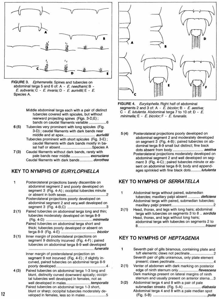
KEY TO NYMPHS OF EPHEMERELLA

Middle abdominal terga each with a pair of prominent upward projecting spines (Figs. 3-

, A ,8) .................... .. .......................................... 2 Middle abdominal terga without such spines, at

most a very small pair of posterior projecting spines (Fig. 3-C) .... ........................................ 3

2 ( 1) Spines long, sharp, and found on segments 1-8 (Fig. 3-A); a pale stripe on abdomen between spines .................... .... ........ ................ needhami

Spines moderately long, sharp, and found on segments 2-9 (Fig. 3-8) ; abdomen without a longitudinal pale stripe .. ....................... sub varia

3 (1) Middle abdominal terga with paired tubercles that often result in a small spine or rearward projec­tion on posterior margin of each tergum ........ .4

Middle abdominal terga without paired tubercles; posterior margin of each tergum straight or evenly curved ................................................. . 7

4 (3) Tibiae and tarsi without dark bands; tail filaments without dark bands ....... ....................... catawba

Tibiae and tarsi with dark bands; tail filaments with or without dark bands ............................. ........ 5

5 (4) Middle abdominal terga each with a pair of small tubercles from which a tiny spine projects rear­ward (Fig. 3-C); caudal filaments with dark bands near middle and at apex ............... ..... ........ ...... ........... in varia or rotunda

(Spines more prominent in rotunda, extremely small in invaria) 11

12

'• II

--..,-------.....,-~~~ /.11 . ( I I 1 1 _ · ,'/; ,),! ~

D E

FIGURE 3. Ephemerel/a. Spines and tubercles on abdominal terga 5 and 6 of: A - E needham/; B -

E subvaria; C - E invaria; 0 - E aurivi/1/i; E - E Species A.

Middle abdominal terga each with a pair of distinct tubercles covered with spicules, but without rearward projecting spines (Figs. 3-D,E) ; bands on caudal filaments variable ................. 6

6 (5) Tubercles very prominent with long spicules (Fig. 3-0) ; caudal filaments with dark bands near middle and at apex ... ............................ aurivillii

Tubercles prominent with short spicules (Fig. 3-E) ; caudal filaments with dark bands mostly in ba-sal half or absent.. ............................. Species A

7 (3) Caudal filaments without dark bands, rarely with pale bands near middle .......... ......... excrucians

Caudal filaments with dark bands ...... ....... dorothea

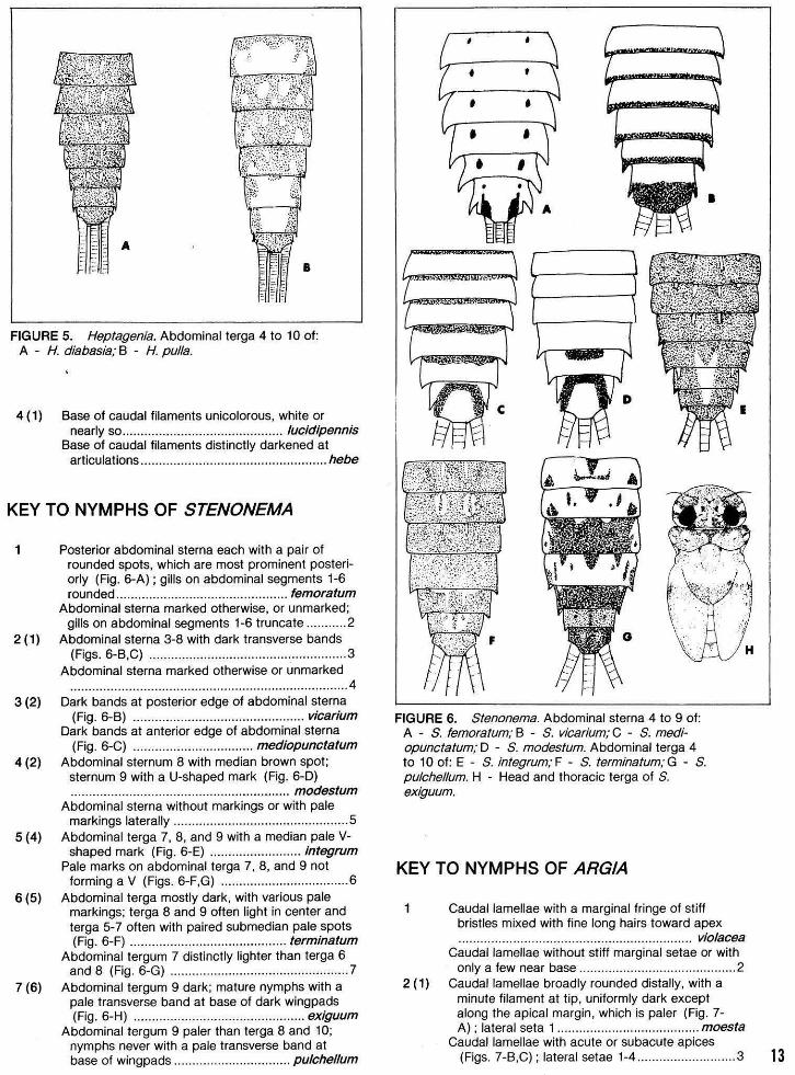
KEY TO NYMPHS OF EURYLOPHELLA

1 Posterolateral projections barely discernible on abdominal segment 2 and poorly developed on segment 3 (Fig. 4-A) ; occipital tubercles minute or absent in both sexes ....................................... 2

Posterolateral projections poorly developed on abdominal segment 2 and very. well developed on segment 3 (Fig. 4-B,C) .................. .................... 3

2 (1) Paired tubercles on abdominal terga long and thin; tubercles moderately developed on terga 8-9 (Fig. 4-0) ....................................... ...... minime/la

Paired tubercles on abdominal terga short and thick; tubercles poorly developed or absent on terga 8-9 (Fig. 4-E) .................................. bico/or

3 (1) Inner margin of posterolateral projections on segment 9 distinctly incurved (Fig. 4-F) ; paired tubercles on abdominal terga 8-9 well developed ...................... ........ .... .............................. funera/is

Inner margin of posterolateral projection on segment 9 not incurved (Fig. 4-E) ; if slightly in­curved, paired tubercles on abdominal terga 8-9 poorly developed .... ..... .... .............. .............. ..... ... 4 .

4 (3) Paired tubercles on abdominal terga 1-3 long and blunt, distinctly curved downward apically; occipi­tal tubercles well developed in females, not as well developed in males ........................ temporalis

Paired tubercles on abdominal terga 1-3 short, blunt or sharp; occipital tubercles moderately de-veloped in females, less so in males .................... 5

I

E

c

FIGURE 4. Eury/ophel/a. Right half of abdominal segments 2 and 3 of: A - E blcolor; B - E aestiva; C - E /utulenta. Abdominal terga 7 to 10 of: 0 - E min/mel/a; E - E bico/or; F - E funeralis.

5 (4) Posterolateral projections poorly developed on abdominal segment 2 and moderately developed on segment 3 (Fig. 4-B) ; paired tubercles on ab­dominal terga 8-9 small but distinct; fine back dots absent from body .............................. aestiva

Posterolateral projections moderately developed on abdominal segment 2 and well developed on seg­ment 3 (Fig. 4-C) ; paired tubercles minute or ab­sent on abdominal terga 8-9; body and append-ages sprinkled with fine black dots .......... lutu/enta

KEY TO NYMPHS OF SERRA TELLA

1 Abdominal terga without paired, submedian tubercles; maxillary pal pi absent ............ de fie/ens

Abdominal terga with paired, submedian tubercles; maxillary pal pi present. .................................. ...... 2

2 ( 1) Head, thorax, and legs with long hairs; abdominal terga with tubercles on segments 3 to 8 .. sordida

Head, thorax, and legs without long hairs; abdominal terga with tubercles on segments 2 to 8 .......................... ..................................... ... frlsoni

KEY TO NYMPHS OF HEPTAGENIA

1 Seventh pair of gills biramous, containing plate and tuft elements; claws not pectinate .. .............. ....... 2

Seventh pair of gills uniramous, only plate element present; claws pectinate ...................................... 4

2 (1) Venter of abdomen with dark marking on posterior edge of ninth sternum only ................... flavescens

Dark markings present on lateral margins of ninth sternum and usually present on anterior sterna ... 3

3 (2) Abdominal terga 4 and 8 with a pair of pale submedian streaks (Fig. 5-A) .............. ... diabasia

Abdominal terga 4 and 8 with a pale median spot (Fig. 5-B) .................. ...... ............... .............. pu/la

A

FIGURE 5. Heptagenia. Abdominal terga 4 to 10 of: A - H. diabasia; B - H. pulla.

4 (1) Base of caudal filaments unicolorous, white or nearly so............................................ lucidipennis

Base of caudal filaments distinctly darkened at articulations ................................................... hebe

KEY TO NYMPHS OF STENONEMA

1 Posterior abdominal sterna each with a pair of rounded spots, which are most prominent posteri­orly (Fig. 6-A); gills on abdominal segments 1-6 rounded ............................................... femora tum

Abdominal sterna marked otherwise, or unmarked; gills on abdominal segments 1-6 truncate ........... 2

2 (1) Abdominal sterna 3-8 with dark transverse bands

(Figs. 6-B,C) ······································:···············3 Abdominal sterna marked otherwise or unmarked

............................................ ..... ........................... 4 3 (2) Dark bands at posterior edge of abdominal sterna

(Fig. 6-B) ...................... ......................... vicarium Dark bands at anterior edge of abdominal sterna

(Fig. 6-C) ................................. mediopunctatum 4 (2) Abdominal sternum 8 with median brown spot;

sternum 9 with a U-shaped mark (Fig. 6-D) ................ ............................................ modestum

Abdominal sterna without markings or with pale markings laterally .... ................... ........ ................. 5

5 (4) Abdominal terga 7, 8, and 9 with a median pale V-shaped mark (Fig. 6-E) ......................... integrum

Pale marks on abdominal terga 7, 8, and 9 not forming a V (Figs. 6-F,G) ............................ ....... 6

6 (5) Abdominal terga mostly dark, with various pale markings; terga 8 and 9 often light in center and terga 5-7 often with paired submedian pale spots (Fig. 6-F) ............................ ............... terminatum

Abdominal tergum 7 distinctly lighter than terga 6 and 8 (Fig. 6-G) ................................................ . 7

7 (6) Abdominal tergum 9 dark; mature nymphs with a pale transverse band at base of dark wingpads (Fig. 6-H) .............. ............... .................. exiguum

Abdominal tergum 9 paler than terga 8 and 10; nymphs never with a pale transverse band at base of wing pads ... ...... ............... ........ pu/chellum

FIGURE 6. Stenonema. Abdominal sterna 4 to 9 of: A - S. femora tum; B - S. vicarium; C - S. medi­opunctatum; D - S. modestum. Abdominal terga 4 to 10 of: E - S. integrum; F - S. terminatum; G - S. pulchellum. H - Head and thoracic terga of S . exiguum.

KEY TO NYMPHS OF ARGIA

1 Caudal lamellae with a marginal fringe of stiff bristles mixed with fine long hairs toward apex ......... ....................................................... violacea

Caudal lamellae without stiff marginal setae or with only a few near base .... .. .. ................................... 2

2 (1) Caudal lamellae broadly rounded distally, with a minute filament at tip, uniformly dark except along the apical margin , which is paler (Fig. 7-A) ; lateral seta 1 ...... ................................. moesta

Caudal lamellae with acute or subacute apices (Figs. 7-B,C); lateral setae 1-4 ................. ......... . 3 13

14

• FIGURE 7. Argia. Lateral caudal lamella of: A - A.

moesta; B - A. apicalis; C - A. tibialis.

3 (2) Lateral setae 2-4; lateral lamellae widest in the middle (Fig. 7-B) ...................................... apica/is

Lateral seta 1; lateral lamellae widest beyond middle (Fig. 7-C) ....................................... tibialis

KEY TO NYMPHS OF NEUROCORDULIA

Pyramidal horn on front of head ................. molest a No distinct horn on front of head ................ ........... 2

2 ( 1) Lateral spines on abdominal segment 9 greatly surpass tips of paraprocts; dorsal hooks blunt and erect ................................................. obso/eta

Lateral spine on abdominal segment 9 barely reaching tips of paraprocts; dorsal hooks blunt and low, slanting to the rear ......... yamaskanensis

KEY TO LARVAE OF BRACHYCENTRUS

1 Head entirely dark ................................................. 2 Head with distinct light markings (Figs. 8-A.B) ..... 3

2 ( 1) First abdominal sternum with 4 setae; metacoxal lobe surrounded by more than 30 setae ...... .................................................... occidentalis

First abdominal sternum with 2 setae; metacoxal lobe surrounded by about 11 setae .... americanus

FIGURE 8. Brachycentrus. Dorsal view of head of: A - B. latera/is; B - B. numerosus.

3 ( 1) Head pale with dark stripes paralleling epicranial sutures, and a median dark stripe on frons (Fig. 8-A) ; pronotum with an anterior dark stripe and a dark stripe along transverse fold .............. latera/is

Front of head mostly dark, with large pale marks laterally on frons (Fig. 8-B); pronotum without distinct transverse stripes .................... numerosus

KEY TO LARVAE OF MICRASEMA

Head dark with pale stripes along frontal sutures and behind eyes; mesonotum with a single seta at SA-1 ... .................... ........ ............................ kluane

Head pale with darker muscle scars; mesonotum with a row of several setae at SA-1 ..................... 2

2 (1) Case of sand grains; head with distinct, dark, rounded muscle scars on back of head, most nearly as large as eye; one or two pairs of pale spots usually on anterior of frontoclypeus (Fig. 9-A) .......... ..................... ............................ rusticum

FIGURE 9 . Micrasema. Dorsal view of head of: A -M. rusticum; B - M. wataga.

Case of fibers of vegetation; muscle scars on back of head highly variable in size and shape, fre­quently contiguous, and often indistinct; anterior of frontoclypeus without large pale spots (Fig. 9-B) ............................................................. wataga

KEY TO LARVAE OF CHIMARRA

Apex of frons with a pair of large. rounded lobes (Fig. 10-A) ..................................... ......... obscura

Apex of frons with smaller lobes, the left lobe not rounded .................................... ........................... 2

2 (1) Basal notch of right mandible very deep, with basal and apical side of notch subequal in length (Fig. 10-E) ; apex of frons with a small, rounded right lobe (Fig. 10-B) ........................................... soc/a

Basal notch of right mandible with apical side much shorter than basal side (Figs. 10-F,G); right lobe on apex of frons larger (Figs. 10-C,D) .. ...... ........................................ .. .... .... ................ .... 3

3 (2) Basal notch of right mandible shallow and forming a right angle (Fig. 10-F); apex of frons usually with a broad notch to the left of the right lobe (Fig. 10-C) ............................................. aterrima

Basal notch of right mandible acute and deep (Fig. 10-G); apex of frons usually with an indistinct or narrow notch to the left of the right lobe (Fig. 10-D) .......... ..................................... .............. .... . feria

KEY TO LARVAE OF HYDROPSYCHE

1 Frontoclypeus with 2 large upturned teeth on anterior margin (Figs. 11-A,B) ........................... 2

Frontoclypeus without 2 large upturned teeth on anterior margin .................................................... 3

2 ( 1) Posterior of head yellow with only a very narrow dark line on stem of epicranial suture (Fig. 11-A); frontoclypeus with a V-shaped pale mark ...... orris

Posterior of head with a broad dark mark along stem of epicranial suture (Fig. 11-B) ; frontoc­lypeus with 2 large anterolateral pale spots ...................................... ....................... ...... bidens

FIGURE 10. Chimarra. Apex of frons of: A - C. ob­scura; 8 - C. socia; C - C. aterrima; D - C. feria. Dorsal view of right mandible of: E - C. socia; F -

C. aterrima; G - C. feria.

3 (1) Anterior edge of frontoclypeus produced (Fig. 11-C); head pattern as in Fig. 11-C ........... phalerata

Anterior edge of frontoclypeus straight or broadly rounded; head pattern otherwise ......................... 4

4 (3) Large spine-like setae, similar to those on sclerotized area of abdominal sternum 9, on ven-ter of anal legs ..................................................... 5

Large spine-like setae absent from venter of anal legs ............................... ...... ................... .. ........ .... 9

5 (4) Frontoclypeus mostly dark, with at most small pale spots (Figs. 11-D,E) .... ...... .. ............................... 6

Frontoclypeus with large pale areas anteriorly (Figs. 11-F,G) .................................................... 8

6 (5) Frontoclypeus brown with 2 pairs of distinct pale spots (Fig. 11-D) ; numerous dark, bristle-like se-tae on posterior of frontoclypeus .. .............. valanis

Frontoclypeus mottled brown with indistinct pale spots (Fig. 11-E) or light brown without spots; pale, spine-like setae on frontoclypeus ................ 7

7 (6) Frontoclypeus mottled brown with indistinct pale spots (Fig. 11-E) ; posterolateral and ventral areas of head pale, with rows of muscle scars be­hind eyes; pronotum with distinct dark areas at base of pale spinelike setae and with large pale muscle scars laterally ............................... sca/aris

Frontoclypeus not mottled with indistinct pale spots; entire head light brown without distinct muscle scars, but with a patch of darker setae

between eye and occiput; pronotum light brown without lateral muscle scars and insertions of pale spine-like setae only slightly darker than background ............................... probably placoda

8 (5) Head with a brown patch on stem of epicranial suture; dark areas of frontoclypeus contiguous (Fig. 11-F); spine-like setae on anal legs same size as those on 9th abdominal sternum .... aerata

FIGURE 11. Hydropsyche. Dorsal view of head of: A - H. orris; 8 - H. bidens; C - H. phalerata; D -

H. valanis; E - H. scalaris; F - H. aerata; G - H. frisoni; H - H. cuanis; I - H. dicantha; J - Lateral view of head of H. Ieonardi. Dorsal view of head of: K - H. Ieonardi; L - H. simulans; M - H. arinale. 15

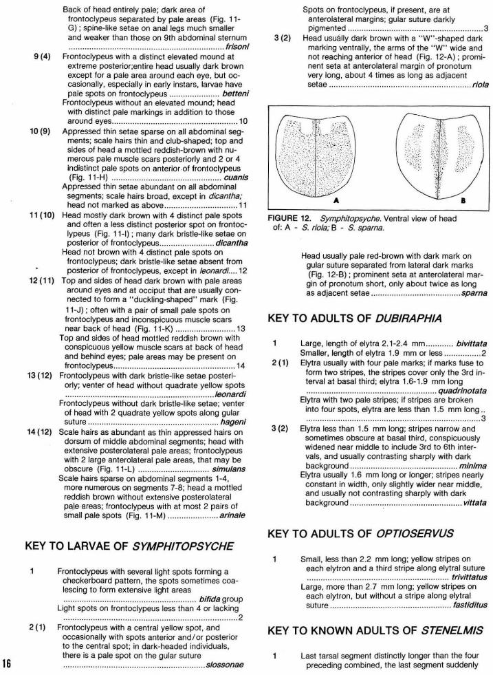
16

Back of head entirely pale; dark area of frontoclypeus separated by pale areas (Fig. 11-G) ; spine-like setae on anal legs much smaller and weaker than those on 9th abdominal sternum .................................................................... frisoni

9 (4) Frontoclypeus with a distinct elevated mound at extreme posterior;entire head usually dark brown except for a pale area around each eye, but oc­casionally, especially in early ins tars, larvae have pale spots on frontoclypeus ... ................... betteni

Frontoclypeus without an elevated mound; head with distinct pale markings in addition to those around eyes .................. ..................... ........ ........ 10

10 (9) Appressed thin setae sparse on all abdominal seg-ments; scale hairs thin and club-shaped; top and sides of head a mottled reddish-brown with nu­merous pale muscle scars posteriorly and 2 or 4 indistinct pale spots on anterior .of frontoclypeus (Fig. 11-H) ................... ............................. cuanis

Appressed thin setae abundant on all abdominal segments; scale hairs broad, except in dicantha; head not marked as above ................................ 11

11 (10) Head mostly dark brown with 4 distinct pale spots and often a less distinct posterior spot on frontoc­lypeus (Fig. 11-1) ; many dark bristle-like setae on posterior of frontoclypeus ........................ dicantha

Head not brown with 4 distinct pale spots on frontoclypeus; dark bristle-like setae absent from posterior of frontoclypeus, except in Ieonardi .... 12

12 ( 11) Top and sides of head dark brown with pale areas around eyes and at occiput that are usually con­nected to form a "duckling-shaped" mark (Fig. 11-J); often with a pair of small pale spots on frontoclypeus and inconspicuous muscle scars near back of head (Fig. 11-K) .............. ............ 13

Top and sides of head mottled reddish brown with conspicuous yellow muscle scars at back of head and behind eyes; pale areas may be present on frontoclypeus ............................... .................. .... 14

13 (12) Frontoclypeus with dark bristle-like setae posteri­orly; venter of head without quadrate yellow spots ..... ............... ......................................... .. .. Ieonardi

Frontoclypeus without dark bristle-like setae; venter of head with 2 quadrate yellow spots along gular suture ......................................................... hagen/

14 (12) Scale hairs as abundant as thin appressed hairs on dorsum of middle abdominal segments; head with extensive posterolateral pale areas; frontoclypeus with 2 large anterolateral pale areas, that may be obscure (Fig. 11-L) ........ ....................... simulans

Scale hairs sparse on abdominal segments 1-4, more numerous on segments 7 -8; head a mottled reddish brown without extensive posterolateral pa!e areas; frontoclypeus with at most 2 pairs of small pale spots (Fig. 11-M) ...................... arinale

KEY TO LARVAE OF SYMPHITOPSYCHE

Frontoclypeus with several light spots forming a checkerboard pattern, the spots sometimes coa­lescing to form extensive light areas ................................ ............ .... .......... bifid a group

Light spots on frontoclypeus less than 4 or lacking ...... ........ ...................... ............... ........................ . 2

2 (1) Frontoclypeus with a central yellow spot, and occasionally with spots anterior and I or posterior to the central spot; in dark-headed individuals, there is a pale spot on the gular suture ......................................... ..................... slossonae

Spots on frontoclypeus, if present, are at anterolateral margins; gular suture darkly pigmented ........... .... ............................................ 3

3 (2) Head usually dark brown with a "W"-shaped dark marking ventrally, the arms of the "W" wide and not reaching anterior of head (Fig. 12-A) ; promi­nent seta at anterolateral margin of pronotum very long, about 4 times as long as adjacent setae .............. ................. .. ......... ............... ..... rio/a

FIGURE 12. Symphitopsyche. Ventral view of head of: A - S. rio/a; 8 - S. sparna.

Head usually pale red-brown with dark mark on gular suture separated from lateral dark marks (Fig. 12-8); prominent seta at anterolateral mar­gin of pronotum short, only about twice as long as adjacent setae ...... ................................. spa rna

KEY TO ADULTS OF DUBIRAPHIA

Large, length of elytra 2.1-2.4 mm ............ blvittata Smaller, length of elytra 1.9 mm or less ................ 2

2 ( 1) Elytra usually with four pale marks; if marks fuse to form two stripes, the stripes cover only the 3rd in­terval at basal third; elytra 1.6-1.9 mm long ......................................................... quadrinotata

Elytra with two pale stripes; if stripes are broken into four spots, elytra are less than 1.5 mm long .. oooooo ooooooooooo oOOO oooooooooo•ooo ooooooooooooooooOOOOO OOOOOOooOOOo oooo••••3

3 (2) Elytra less than 1o5 mm long; stripes narrow and sometimes obscure at basal third, conspicuously widened near middle to include 3rd to 6th inter­vals, and usually contrasting sharply with dark background 0. 0 ............... 0. 0 ................ ........ 0 0 minima

Elytra usually 1.6 mm long or longer; stripes nearly constant in width, only slightly wider near middle, and usually not contrasting sharply with dark background ............ 00 : .... ....... ...................... 0 vittata

KEY TO ADULTS OF OPT/OSERVUS

1 Small, less than 202 mm long; yellow stripes on each elytron and a third stripe along elytral suture . 0 0 ........ 0 ... 0. 0. 0. 0. 0 ...... 0 0 0. 0. 0 0 ................... 0 0 0 0. trivittatus

Large, more than 2.7 mm long; yellow stripes on each elytron, but without a stripe along elytral suture ...... 0. 0 .... 0. 0. 0 ... .. 0 .... 0. 0 0 ............ 0 ........ fastlditus

KEY TO KNOWN ADULTS OF STENELM/S

1 Last tarsal segment distinctly longer than the four preceding combined, the last segment suddenly

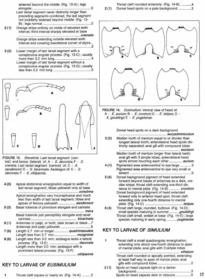
widened beyond the middle (Fig. 13-A); legs elongate .............................................................. 6

Last tarsal segment never distinctly longer than preceding segments combined, the last segment not suddenly widened beyond middle (Fig. 13-B) ; legs normal ................................................... 2

2 ( 1) Orange stripe entirely on inside of elevated sixth interval; third interval sharply elevated at base .............. .. ................................................ cremata

Orange stripe extending outside elevated sixth interval and covering basolateral corner of elytra .. ............................................................................ 3

3 (2) Lower margin of last tarsal segment with a conspicuous angular process (Fig. 13-C); usually more than 3.2 mm long ............................. ........ .4

Lower margin of last tarsal segment without a conspicuous angular process (Fig. 13-D); usually less than 3.2 mm long ........................................ 5

v. E

FIGURE 13. Stenelmis. Last tarsal segment (ven­tral) and tarsus (lateral) of: A - S. decorata; F - S. crena/a. Last tarsal segment (ventral) of: C - S. sandersom;· D - S. bicarinata. Aedeagus of: E - S. decorata; F - S. vittipennis.

4 (3) Apical abdominal emargination equal to width of last tarsal segment; tibiae yellowish only at base ....... .... .... ........ ........ ...... ............. ............. concinna

Apical emargination very inconspicuous and much less than width of last tarsal segment; tibiae and apices of femora yellowish .................. sandersoni

5 (3) Basal tubercle of pronotum elongate and carinate ..................................................................... mera

Basal tubercle just perceptibly elongate and never carinate ................................................ bicarinata

6 (1) Antennae or pal pi, or both, dark brown or black ... 7 Antennae and palpi yellowish ................................ 8

7 (6) Length 2.7 mm or longer ............... quadrimaculata Length less than 2.7 mm ........................ musgravei

8 (6) Length less than 3.0 mm; aedeagus lacks a lateral process (Fig. 13-E) ......... .... ................. . decorata

Length more than 3.0 mm; aedeagus with a prominent lateral process (Fig. 13-F) . . . . . . . . . . . . . . . . . . . . . . . . . . . . . . . . . . . . . . . . . . . . . . . . . . . . . . . . . . . . . vittipennis

KEY TO LARVAE OF EUSIMUL/UM

1 Throat cleft square or nearly so (Fig. 14-A} ......... 2

Throat cleft rounded anteriorly (Fig. 14-B) .......... .4 2 ( 1) Dorsal head spots on a pale background .............. 3

FIGURE 14. Eusimulium. Ventral view of head of: A - E aurium; B - E croxtoni; C - E talipes; D -

E gouldingi; E - E pugetense.

Dorsal head spots on a dark background ....................... ........................... euryadminiculum

3 (2) Median tooth of mentum equal to or shorter than longest lateral tooth; anterolateral head spots dis­tinctly separated; anal gill with compound lobes ................................................................ excisum

Median tooth of mentum longer than lateral teeth; anal gill with 3 simple lobes; anterolateral head spots almost touching each other ............. aurium

4 (1) Pigmented area anteroventral to eye large .. .......... 5 Pigmented area anteroventral to eye very small or

absent ................................................................. 6 5 (4) Dorsal background pigment of head extended

forward beyond bases of antennae as a dark, me­dian stripe; throat cleft extending one-third dis-tance to mental plate (Fig. 14-B) ........... croxtoni

Dorsal background pigment of head extended forward only to anterior head spot; throat cleft extending only one-fourth distance to mental plate (Fig. 14-C) ....................................... latipes

6 (4) Throat cleft large, rounded, bulbous (Fig. 14-D) ; small species maturing in summer .......... gouldingi

Throat cleft small, widest at base (Fig. 14-E); large species maturing in early spring ........... pugetense

KEY TO LARVAE OF SIMULIUM

1 Throat cleft a small quadrangular emargination, extending only about one-fourth distance to apex of mental plate; anal gills with 3 simple lobes .............. ........... ...................................... . vittatum

Throat cleft rounded or apically pointed, extending at least half way to apex of mental plate; anal gills with compound lobes ............ ........ ........ .. ..... 2

2 ( 1) Spots on head capsule light on a darker background .............................. ........ ....... ............ 3

Spots on head capsule dark or obscure ................ 5 17

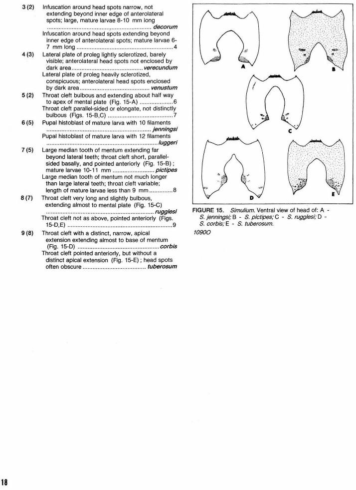
18

3 (2) lnfuscation around head spots narrow, not extending beyond inner edge of anterolateral spots; large, mature larvae 8-10 mm long .... ................................ ............. .............. decorum

lnfuscation around head spots extending beyond inner edge of anterolateral spots; mature larvae 6-7 mm long .......................................................... 4

4 (3) Lateral plate of proleg lightly sclerotized, barely visible; anterolateral head spots not enclosed by dark area ........................................... verecundum

Lateral plate of proleg heavily sclerotized, conspicuous; anterolateral head spots enclosed by dark area ........................ ...... ............ venus tum

5 (2) Throat cleft bulbous and extending about half way to apex of mental plate (Fig. 15-A) ............. .. ..... 6

Throat cleft parallel-sided or elongate, not distinctly bulbous (Figs. 15-B,C) ................... ............ ........ 7

6 (5) Pupal histoblast of mature larva with 10 filaments ............................ ................................... jennings!

Pupal histoblast of mature larva with 12 filaments ........... ........................................................ lugger!

7 (5) Large median tooth of mentum extending far beyond lateral teeth; throat cleft short, parallel­sided basally, and pointed anteriorly (Fig. 15-B) ; mature larvae 10-11 mm ......................... pictipes

Large median tooth of mentum not much longer than large lateral teeth; throat cleft variable; length of mature larvae less than 9 mm ............. . 8

8 (7) Throat cleft very long and slightly bulbous, extending almost to mental plate (Fig. 15-C) ............................. .................................... rugglesi

Throat cleft not as above, pointed anteriorly (Figs. 15-D,E) ............................................... ................ 9

9 (8) Throat cleft with a distinct, narrow, apical extension extending almost to base of mentum (Fig. 15-D) ............................ ..................... corbis

Throat cleft pointed anteriorly, but without a distinct apical extension (Fig. 15-E) ; head spots often obscure ........................... .......... . tuberosum

FIGURE 15. Simulium. Ventral view of head of: A -S. jennings!; B - S. plctipes; C - S. rugglesi; D -S. corbis; E - S. tuberosum.

10900

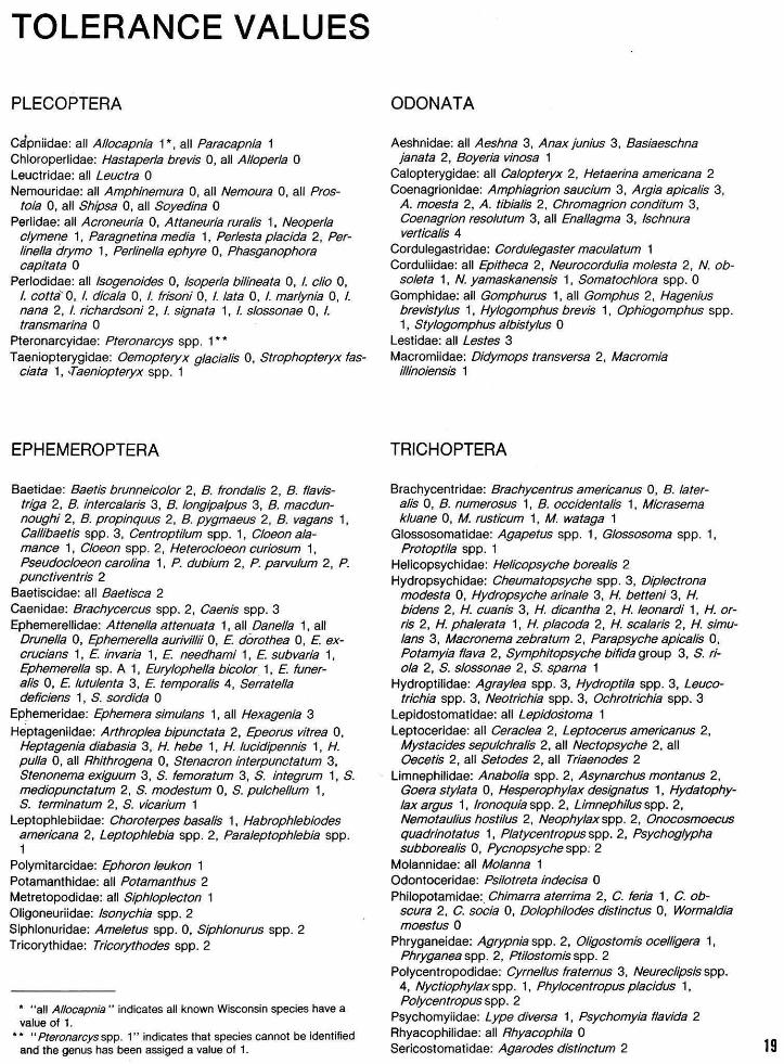
TOLERANCE VALUES

PLECOPTERA

Cdpniidae: all Al/ocapnia 1 *, all Paracapnia 1 Chloroperlidae: Hastaperla brevis 0, all Alloperla 0 Leuctridae: all Leuctra 0 Nemouridae: all Amphinemura 0, all Nemoura 0, all Pros­

toia 0, all Shipsa 0, all Soyedina 0 Perlidae: all Acroneuria 0, Attaneuria ruralis 1, Neoperla

clymene 1, Paragnetina media 1, Perlesta placida 2, Per­linella drymo 1, Perlinella ephyre 0, Phasganophora capitata 0

Perlodidae: all lsogenoides 0, !soper/a bilineata 0, I. clio 0, I. cotta' 0, I. dicala 0, I. frisoni 0, I. lata 0, I. mar/ynia 0, I. nana 2, /. richardsoni 2, /. signata 1, I. slossonae 0, I. transmarina 0

Pteronarcyidae: Pteronarcys spp. 1 * * Taeniopterygidae: Oemopteryx glacia/is 0, Strophopteryx fas­

ciata 1, -Taeniopteryx spp. 1

EPHEMEROPTERA

Baetidae: Baetis brunneicolor 2, B. frondalis 2, B. f/avis­triga 2, B. interca/aris 3, B. longipalpus 3, B. macdun­noughi 2, B. propinquus 2, B. pygmaeus 2, B. vagans 1, Callibaetis spp. 3, Centroptilum spp. 1, C/oeon ala­mance 1, Cloeon spp. 2, Heterocloeon curiosum 1, Pseudocloeon carolina 1, P. dubium 2, P. parvulum 2, P. punctiventris 2

Baetiscidae: all Baetisca 2 Caenidae: Brachycercus spp. 2, Caenis spp. 3 Ephemerellidae: Attenella attenuata 1, all Danella 1, all

Drunella 0, Ephemerella aurivillii 0, £ dorothea 0, £ ex­crucians 1 , £ invaria 1 , £ needhami 1, £ subvaria 1 , Ephemerel/a sp. A 1, Eurylophel/a bico/or 1, £ tuner­a/is 0, £ lutulenta 3 , £ temporalis 4, Serratella deficiens 1, S. sordida 0

Ephemeridae: Ephemera simulans 1, all Hexagenia 3

Heptageniidae: Arthroplea bipunctata 2, Epeorus vitrea 0, Heptagenia diabasia 3, H. hebe 1, H. lucidipennis 1, H. pul/a 0, all Rhithrogena 0, Stenacron interpunctatum 3, Stenonema exiguum 3, S. femoratum 3, S. integrum 1, S. mediopunctatum 2, S. modestum 0, S. pulchellum 1, S. terminatum 2, S. vicarium 1

Leptophlebiidae: Choroterpes basalis 1, Habrophlebiodes americana 2, Leptophlebia spp. 2, Paraleptophlebia spp. 1

Polymitarcidae: Ephoron leukon 1 Potamanthidae: all Potamanthus 2 Metretopodidae: all Siphloplecton 1 Oligoneuriidae: lsonychia spp. 2 Siphlonuridae: Ameletus spp. 0, Siph/onurus spp. 2 Tricorythidae: Tricorythodes spp. 2

* "all Allocapnia " indicates all known Wisconsin species have a value of 1.

* * "Pteronarcys spp. 1" indicates that species cannot be identified and the genus has been assiged a value of 1.

ODONATA

Aeshnidae: all Aeshna 3, Anax junius 3, Basiaeschna janata 2, Boyeria vinosa 1

Calopterygidae: all Calopteryx 2, Hetaerina americana 2 Coenagrionidae: Amphiagrion saucium 3, Argia apicalis 3,

A. moesta 2, A. tibialis 2, Chromagrion conditum 3, Coenagrion resolutum 3 , all Enallagma 3, lschnura vertica/is 4

Cordulegastridae: Cordulegaster maculatum 1 Corduliidae: all Epitheca 2, Neurocordu/ia mo/esta 2, N. ob­

soleta 1, N. yamaskanensis 1, Somatoch/ora spp. 0 Gomphidae: all Gomphurus 1, all Gomphus 2, Hagenius

brevistylus 1, Hylogomphus brevis 1, Ophiogomphus spp. 1, Stylogomphus albisty/us 0

Lestidae: all Lestes 3 Macromiidae: Didymops transversa 2, Macromia

illinoiensis 1

TRICHOPTERA

Brachycentridae: Brachycentrus americanus 0, B. later­a/is 0, B. numerosus 1. B. occidentalis 1, Micrasema kluane 0, M. rusticum 1, M. wataga 1

Glossosomatidae: Agape/us spp. 1, G/ossosoma spp. 1, Protoptila spp. 1

Helicopsychidae: Helicopsyche borealis 2 Hydropsychidae: Cheumatopsyche spp. 3, Diplectrona

modes/a 0, Hydropsyche arinale 3, H. betteni 3, H. bidens 2, H. cuanis 3, H. dicantha 2, H. Ieonardi 1, H. or­ris 2, H. phalerata 1, H. placoda 2, H. scalaris 2, H. simu­lans 3, Macronema zebratum 2, Parapsyche apicalis 0, Potamyia flava 2, Symphitopsyche bifida group 3, S. ri­o/a 2, S. slossonae 2, S. sparna 1

Hydroptilidae: Agray/ea spp. 3, Hydroptila spp. 3, Leuco­trichia spp. 3, Neotrichia spp. 3, Ochrotrichia spp. 3

Lepidostomatidae: all Lepidostoma 1 Leptoceridae: all Ceraclea 2, Leptocerus americanus 2,

Mystacides sepulchralis 2, all Nectopsyche 2, all Oecetis 2, all Setodes 2, all Triaenodes 2

Limnephilidae: Anabo/ia spp. 2, Asynarchus montanus 2, Goera stylata 0, Hesperophylax designatus 1, Hydatophy­lax argus 1, lronoquia spp. 2, Limnephi/us spp. 2, Nemotau/ius hostilus 2, Neophy/ax spp. 2, Onocosmoecus quadrinotatus 1, Platycentropus spp. 2, Psychog/ypha subborealis 0, Pycnopsyche spp: 2

Molannidae: all Molanna 1 Odontoceridae: Psilotreta indecisa 0 Philopotamidae:. Chimarra aterrima 2, C. feria 1, C. ob­

scura 2, C. socia 0, Dolophilodes distinctus 0, Wormaldia moestus 0

Phryganeidae: Agrypniaspp. 2, 0/igostomis ocelligera 1, Phryganea spp. 2, Ptilostomis spp. 2

Polycentropodidae: Cyme/Ius fraternus 3, Neureclipsis spp. 4, Nyctiophylax spp. 1, Phy/ocentropus placidus 1, Po/ycenuopusspp.2

Psychomyiidae: Lype diversa 1, Psychomyia flavida 2 Rhyacophilidae: all Rhyacophila 0 Sericostomatidae: Agarodes distinctum 2 19

20

MEGALOPTERA

Corydalidae: all Chauliodes 2, Corydalis cornutus 2, Nigronia serricornis 1

Sialidae: Sialis spp. 2

LEPIDOPTERA

Pyralidae: Neocatac/ysta spp. 1, Nymphula spp. 1, Paraponyx spp. 1, Parargyractis spp. 2

COLEOPTERA

Dryopidae: all Helichus 2 Elmidae: Ancyronyx variegata 2, Dubiraphia bivittata 2, D.

minima 3, D. quadrinotata 3, D. vittata 3, Dubiraphia lar­vae 3, Macronychus glabratus 2, Microcy/loepus pusillus 1, Optioservus fastiditus 2, 0. trivittatus 1, Optioservus larvae 2, Stenelmis bicarinata 2, S. crenata 3, S. decorata 2, S. musgravei 3, S. sanderson/ 2, S. vittipen­nis 2, Stenelmis larvae 3

Gyrinidae: Dineutus larvae 2, Gyrinus larvae 2 (Do not count adults)

Psephenidae: Ectopria spp. 2, Psephenus herrick/ 2 (Do not include adults or larvae of Dytiscidae, Haliplidae or Hydrophilidae)

DIPTERA

Athericidae: Atherlx variegate 2 Blepharoceridae: 8/epharocera spp. 0 Ceratopogonidae: Atrichopogon spp. 1, Bezzia spp. 3, Cu/i­

coides spp. 4, Monohelea spp. 3, Palpomyia spp. 3, Probezzia spp. 3

Chaoboridae: all Chaoborus 4 Chironomidae: Ablabesmyia spp. 3, Acricotopus spp. 4,

Brill/a spp. 3, Cardiocladius spp. 3 , Chaetocladius spp. 3, Chironomus spp. 5, Cladopelma spp. 4, C/adotanytarsus spp. 3, Cllnotanypus spp. 3, Coelotanypus spp. 2, Cordites spp. 2, Corynoneura spp. 2, Cricotopus spp. 4, Cryptochironomus spp. 4, Cryptotendipes spp. 3, Demicryptochironomus spp. 3 , Diamesa spp. 2, Dicrotendipes spp. 4 Diploe/ad/us spp. 4, Einfeldia spp. 5, Endochironomus spp. 3, Epoicocladius spp. 2, Eukieffer­iella spp. 2, Glyptotendipes spp. 5, Guttipelopia spp. 3, Harnischia spp. 4, Heterotrissocladius spp. 2,

Hydrobaenus spp. 2, Kiefferulus spp. 4, Larsia spp. 3, Limnophyes spp. 3, Microchironomus spp. 4, Microcricotopus spp. 3, Micropsectra spp. 3, Microtendipes spp. 3, Nanocladius spp. 1, Natarsia spp. 3, Nilotanypus spp. 3, Odontomesa spp. 2, Orthocladius spp. 3, Pagastia spp. 2, Parachironomus spp. 4, Parac/adopelma spp. 3, Para/auterborniella spp. 3 , Parametriocnemus spp. 3, Pamtanytarsus spp. 3, Paratendipes spp. 2, Pentaneura spp. 2 , Phaenopsectra spp. 4, Polypedilum spp. 3, Potthastia spp. 2, Procladius spp. 3, Prodiamesa spp. 2, Psectrocladius spp. 2, Psec­trotanypus spp. 3, Pseudochironomus spp. 3, Pseudorthocladius sp. 2, Rheocricotopus spp. 3, Rhe­otanytarsus spp. 3, Saetheria spp. 2, Smittia spp. 4, Stempellina spp. 2, Stempellinella spp. 2, Stenochiro­nomus spp. 2, Stictochironomus spp. 3, Sympotthastia spp. 2 , Tanypus spp. 4, Tanytarsus spp. 3, Thienemanniel­/a spp. 2, Thienemannimyia complex 3, Xenochironomus spp. 2, Zalutschia spp. 2, Zavrelimyia spp. 4

Dolichopodidae: all genera 2 Empididae: all genera 3 Ephydridae: all genera 3 Muscidae: all genera 2 Psychodidae: Pericoma spp. 5, Psychoda spp. 5 Ptychopteridae: Ptychoptera spp. 3 Simuliidae: Cnephia dacotensis 1, Ectemnia taeniatifrons 1,

Eusimulium aurium 2, E croxtoni 1, E eury-adminiculum 1, E johannseni 1, E /at/pes 2, all Prosimu­lium 1, Simulium corbis 0, S. jennings/ 2, S. lugger/ 1, S. tuberosum 2, S. venustum 3, S. verecundum 3, S. vii­tatum 4, Stegopterna mutata 2

Syrphidae: Chrysogasterspp. 5, Eristalisspp . 5, Helophilus spp. 5

Tabanidae: Chrysopsspp. 3, Tabanusspp . 3 Tipulidae: Antocha spp. 2, Dicranota spp. 2, Erioptera spp.

3, He/ius spp. 3, Hesperoconopa spp. 1, Hexatoma spp. 3, Limon/a spp. 2, Limnophila spp. 2, Pedicia spp. 2, Pi/aria spp. 3, Pseudolimnophila spp. 1, Tlpu/a spp. 2

(Do not include Culicidae, Dixidae, or Stratiomyidae)

AMPHIPODA

Gammaridae: Crangonyx gracilis 4, Gammarus pseudolimneus 2

Talitridae: Hyallela azteca 4

ISOPODA

Asellidae: Asel/us intermedius 5

I

RECENT SYNONYMS

EPHEMEROPTERA

ODONATA

TRICHOPTERA

DIPTERA

New Name

Baetis flavistriga Baetis longipa/pus Baetis propinquus Macdunnoa persimplex Stenonema femoratum Stenonema modestum Stenonema terminatum Stenonema vicarium Attenella attenuata Danella Drunella Eurylophella Serrate/fa

Epitheca

Symphitopsyche

Athericidae Brundinella C/adopelma

Hydrobaenus Macropelopia Microchironomus Nanocladius Prodiamesinae Zalutschia Ectemnia taeniatifrons Stegopterna

Old Name

Baetis lev/tans or Baetls phoebus Baetis propinquus Baetis spinosus Stenonema persimplex Stenonema tripunctatum Stenonema rubrum Stenonema bipunctatum Stenonema fuscum Ephemerella attenuata Ephemerella (in part) Ephemerella (In part) Ephemerella (In part) Ephemerella (in part)

Epicordulia or Tetragoneuria

Hydropsyche (In part)

Rhagionldae Psectrotanypus (in part) Cryptocladopelma (in part) Harnischia (in part) Trlssocladius Psectrotanypus Cladopelma Plecopteraco/uthus Diameslnae (in part) Rheocricotopus (in part) Cnephia taeniatifrons Cnephia (in part)

CALCULATION AND EVALUATION OF BIOTIC INDEX VALUES

After all the necessary identifications have been com­pleted, the number of arthropods in each species (or genus) is multipled by the tolerance value for the species (or genus), and the sum of these products is divided by the number of arthropods in the entire sample to obtain the biotic index for the stream

N

Samples obtained between October and May give the most reliable values and can be evaluated according to Table 7 . Accurate correction factors for values obtained from summer samples have not yet been worked out , but the results in Ta­ble 5 suggest that subtracting 0.6 from biotic index values ob­tained in July and August is not unreasonable. A smaller cor­rection factor will be needed for June and September samples.

TABLE 7. Evaluation of water quality using biotic in­dex values of samples collected between October and May.

Biotic Index Water Quality Degree of Organic Pollution

0.00 - 1. 75 Excellent 1.76- 2.25 Very good 2.26 - 2.75 Good 2.76- 3.50 Fair 3.51 - 4.25 Poor 4.26 - 5.00 Very Poor

No organic pollution Possible slight organic pollution Some organic pollution Significant organic pollution Very significant organic pollution Severe organic pollution

The occur renee of several Caenis spp., Cheumatopsycne spp., and Symphitopsyche bifida group, all of which have a tolerance value of 3, will produce abnormally high biotic index values for very clean streams .Calculation of a second biotic index after excluding these three genera is recommended, and if it is below 2.00 it should be used to evaluate the stream. 21

I

RECENT SYNONYMS

EPHEMEROPTERA

ODONATA

TRICHOPTERA

DIPTERA

New Name

Baetis flavistriga Baetis longipa/pus Baetis propinquus Macdunnoa persimplex Stenonema femoratum Stenonema modestum Stenonema terminatum Stenonema vicarium Attenella attenuata Danella Drunella Eurylophella Serrate/fa

Epitheca

Symphitopsyche

Athericidae Brundinella C/adopelma

Hydrobaenus Macropelopia Microchironomus Nanocladius Prodiamesinae Zalutschia Ectemnia taeniatifrons Stegopterna

Old Name

Baetis lev/tans or Baetls phoebus Baetis propinquus Baetis spinosus Stenonema persimplex Stenonema tripunctatum Stenonema rubrum Stenonema bipunctatum Stenonema fuscum Ephemerella attenuata Ephemerella (in part) Ephemerella (In part) Ephemerella (In part) Ephemerella (in part)

Epicordulia or Tetragoneuria

Hydropsyche (In part)

Rhagionldae Psectrotanypus (in part) Cryptocladopelma (in part) Harnischia (in part) Trlssocladius Psectrotanypus Cladopelma Plecopteraco/uthus Diameslnae (in part) Rheocricotopus (in part) Cnephia taeniatifrons Cnephia (in part)

CALCULATION AND EVALUATION OF BIOTIC INDEX VALUES

After all the necessary identifications have been com­pleted, the number of arthropods in each species (or genus) is multipled by the tolerance value for the species (or genus), and the sum of these products is divided by the number of arthropods in the entire sample to obtain the biotic index for the stream

N

Samples obtained between October and May give the most reliable values and can be evaluated according to Table 7 . Accurate correction factors for values obtained from summer samples have not yet been worked out , but the results in Ta­ble 5 suggest that subtracting 0.6 from biotic index values ob­tained in July and August is not unreasonable. A smaller cor­rection factor will be needed for June and September samples.

TABLE 7. Evaluation of water quality using biotic in­dex values of samples collected between October and May.

Biotic Index Water Quality Degree of Organic Pollution

0.00 - 1. 75 Excellent 1.76- 2.25 Very good 2.26 - 2.75 Good 2.76- 3.50 Fair 3.51 - 4.25 Poor 4.26 - 5.00 Very Poor

No organic pollution Possible slight organic pollution Some organic pollution Significant organic pollution Very significant organic pollution Severe organic pollution

The occur renee of several Caenis spp., Cheumatopsycne spp., and Symphitopsyche bifida group, all of which have a tolerance value of 3, will produce abnormally high biotic index values for very clean streams .Calculation of a second biotic index after excluding these three genera is recommended, and if it is below 2.00 it should be used to evaluate the stream. 21

LITERATURE CITED

Beck, W.M. Jr. 1955. Suggested method for reporting biotic data. Sewage Ind. Wastes 27:1193-7.

• Cairns, J. Jr. and K.L. Dickson (Eds.) 1973. Biological meth­ods for the assessment of water quality. Spec. Tech. Publ. Am. Soc. for Testing and Materials. No. 528. Philadelphia. vii

256 pp.

Caspers, M. and L. Karbe 1966. Trophie und Saprobitat als Stoffwechseldynamischer Komplex. Gesichtspuncte fur die Definition der Saprobitatsstufen. Arch. Hydrobiol. 61 :453-70.

1 Chandler, J.R. 1970. A biological approach to water quality managment. Water Poll. Control 4:415-22.

Chutter, F.M. 1972. An empirical biotic index of the quality of water in South African streams and rivers. Water Resour. 6:19-30.

. ... / 1 Cook, S.E.K. 1976. Quest for an index of community structure sensitive to water pollution. Environ. Poll. 11 :269-88.

I Gaufin, A.A. 1973. Use of aquatic invertebrates in the assess­ment of water quality. pp. 96-116 in Cairns and Dickson 1~73).

Hilsenhoff, W.L. 1969. An artificial substrate device for sam­pling benthic stream invertebrates. Limnol. Oceanog. 14:465-71 . 1972. Aquatic insects of the Pine-Popple River, Wisconsin. I. Sampling sites and procedures. Wis. Dep. Nat. Resour. Tech. Bull. No. 54:2-8.

-=- 1 1977. Use of arthropods to evaluate--water quality of streams. Wis. Dep. Nat. Resour. Tech. Bull. No. 100:1-15. 1981 . Aquatic insects of Wisconsin 1 Keys to Wisconsin gen­era and notes on biology, distribution and species. Publ. Nat. Hist. Council Univ. Wis.-Madison No. 2. 60 pp.

22

Holsinger, J.R. 1972. The freshwater amphipod crustaceans (Gammaridae) of North America. Biota of freshwater eco­systems, U.S. Envir. Prot. Agency ldent. Man. No. 5. Wash­ington, D.C. 89 pp.

Howmiller, R.P. and M.A. Scott. 1977. An environmental index based on relative abundance of oligochaete species. J. Water Poll. Cont. Fed. 49:809-15.

Hughes, B.D. 1978. The influence of factors other than pollu­tion on the value of Shannon's diversity index for benthic macro-invertebrates in streams. Water. Res. 12:359-64.

I Hynes, H.B.N. 1960. The biology of polluted waters. Univ. To­ronto Press, Toronto and Buffalo. xiv 202 pp.

Kaesler, R.L. and E.E. Herricks. 1976. Analysis of data from biological surveys of streams: diversity and sample size. Water Resour. Bull. 12 (6) :125-35.

Mason, W.T., Jr., J.B. Anderson, and G.E. Morrisson. 1967. Limestone-filled, artificial substrate sampler-float unit for col­lecting macroinvertebrates in large streams. Prog. Fish-Cult. 29:74.

Murphy, P.M. 1978. The temporal variability in biotic indices. Envir. Poll. 17:227-36.

Pantie, A. and H. Buck. 1955. Die Biologische uberwachund der Gewasser und die Darstellung der Ergebnisse. Gas und Wasserfach. 96:604.

Resh, V.H. and J.D. Unzicker. 1975. Water quality monitoring and aquatic organisms: the importance of species identifica­tion. J. Water Poll. Cont. Fed. 47:9-19.

Roback, S.S. 1974. Chapter 10, Insects (Arthropoda: In­secta). pp. 313-76 in C. W. Hart, Jr. and L.M. Fuller. Eds. 1974. Pollution ecology of freshwater invertebrates. Acad. Press, N.Y., San Francisco, London. 389 pp.

Sladecek, V. 1973. System of water quality from the biological point of view. Ergebnisse der Limnologie 7:1-218.

Weber, C.l. (Ed.) 1973. Biological field and laboratory meth­ods for measuring the quality of surface waters and effluents. U.S. Env. Prot. Agency 67014-73-001 Macroinvertebrates pp. 10-11 .

Wilhm, J.L. 1970. Range of diversity index in benthic macroinvertebrate populations. J. Water Poll. Cont. Fed. 42:A 221-24.

Williams, W.D. 1972. Freshwater isopods (Asellidae) of North America. Biota of freshwater ecosystems, U.S. Env. Prot. Agency ldent. Man. No.7. Washington, D.C. 45 pp.

t Winget; R.N. and F.A. Mangum. 1979. Biotic condition index: integrated biological, physical and chemical stream parame­ters for management. U.S. For. Serv. Intermountain Reg. pp. 1-51.

Zand, S.M. 1976. Indexes associated with information theory in water quality. J. Water Poll. Cont. Fed. 48:2020-31 .

/

89063452734

JJ~~~~mll~~~~~~~~~ b89063452734a

DATE DUE

·- L

nc:T'1R\CAl soc\Eif 1>11'11. c f W15CO~ [:>IN ......

.. ' lb :>~=, .. .: 1.~06 -··-· ·~

- = -

JAN 2~ 1987 lllN R Rf.:f' 'fl

. ' . :".A'! .1 • ~., ,:1 ·~

- :·::{:" .......

MAR ' ,. t': .•• ~

' l1E'& C) C) 1DQ~ I.,..,.. kl-

. . \'"' MAY ~i ,·.;:;,;,

_2ft'f : ii ~'..' ' ~ '! 'lS99 .L.

J

, DEMCO 38-297

ACKNOWLEDGMENTS

Research supported by the College of Agricultural and Life Sciences, University of Wisconsin, Madison, and by the Wis­consin Department of Natural Resources in cooperation with the U.S. Environmental Protection Agency.

About the Author Dr. Hilsenhoff is Professor of Entomology, University of

Wisconsin, Madison.

Production Credits:

Ruth L. Hine, Editor Jane Ruhland and Lori Goodspeed, Copy Editors Richard G. Burton, Layout Artist Susan Steinhoff, Word Processor

TECHNICAL BULLETINS (1977- 1982) 111111111111111 111111 111111 1111 111 1111111

88906345273·

No. 96 Northern pike production in managed spawning and rearing marshes. (1977) Don M. Fago

No. 98 Effects of hydraulic dredging on the ecology of na­tive trout populations in Wisconsin spring ponds. (1977) Robert F. Carline and Oscar M. Brynildson

No. 101 Impact upon local property taxes of acquisitions within the St. Croix River State Forest in Burnett and Polk counties. (1977) Monroe H. Rosner

No. 103 A 15-year study of the harvest, exploitation, and mortality of fishes in Murphy Flowage, Wisconsin. (1978) Howard E. Snow

No. 104 Changes in population density, growth, and har­vest of northern pike in Escanaba Lake after im­plementation of a 22-inch size limit. (1978) James J. Kempinger and Robert F. Carline

No. 105 Population dynamics, predator-prey relationships and management of the red fox in Wisconsin. (1978) Charles M. Pils and Mark A. Martin

No. 106 Mallard population and harvest dynamics in Wis­consin. (1978) James R. March and Richard A. Hunt

No. 107 Lake sturgeon populations, growth, and exploita­tion in Lakes Poygan, Winneconne, and Lake Butte des Morts, Wisconsin. (1978) Gordon R. Priegel and Thomas L. Wirth

No. 109 Seston characterization of major Wisconsin rivers (slime survey). (1978) Joseph R. Ball and David W. Marshall

No. 110 The influence of chemical reclamation on a small brown trout stream in southwestern Wisconsin. (1978) Eddie L. Avery

No. 112 Control and management of cattails in southeast­ern Wisconsin wetlands. (1979) John D. Beule

No. 113 Movement and behavior of the muskellunge de­termined by radio-telemetry. (1979) Michael P. Dombeck

No. 115 Removal of woody stream bank vegetation to im­prove trout habitat. (1979) Robert L. Hunt

No. 116 Characteristics of scattered wetlands in relation to duck production in southeastern Wisconsin. (1979) William E. Wheeler and James R. March

No. 117 Management of roadside vegetative cover by se­lective control of undesirable vegetation. (1980) Alan J. Rusch, Donald R. Thompson, and Cyril Kabat

Copies of the above publications and a complete list of all technical bulletins in the series are available from the Bu­reau of Research, Department of Natural Resources, Box 7921, Madison, WI 53707.

No. 118 Ruffed grouse density and habitat relationships in Wisconsin. (1980) John F. Kubisiak, John C. Moulton, and Keith R. McCaffery

No. 119 A successful application of catch and release regu­lations on a Wisconsin trout stream. (1981) Rob­ertL. Hunt

No. 120 Forest opening construction and impacts in north­ern Wisconsin. (1981) Keith R. McCaffery, James E. Ashbrenner, and John C. Moulton

No. 121 Population dynamics of wild brown trout and as­sociated sport fisheries in four central Wisconsin streams. (1981) Ed L. Avery and Robert L. Hunt

No. 122 Leopard frog populations and mortality in Wis­consin, 1974-76. (1981) Ruth L. Hine, Betty L. Les, and Bruce F. Hellmich

No. 123 An evaluation of Wisconsin ruffed grouse surveys. (1981) Donald R. Thompson and John C. Moulton

No. 124 A survey of Unionid mussels in the Upper Missis­sippi River (Pools 3 through 11). (1981) Pamella A. Thiel

No. 125 Harvst, age structure, survivorship, and produc­tivity of red foxes in Wisconsin, 1975-78. (1981) Charles M. Pils, Mark A. Martin, and Eugene L. Lange

No. 126 Artificial nesting structures for the double-crested cormorant. (1981) Thomas I. Meier

No. 127 Population dynamics of young-of-the-year blue­gill. (1982) Thomas D. Beard

No. 128 Habitat development for bobwhite quail on pri­vate lands in Wisocnsin. (1982) Robert T. Dumke

No. 129 Status and management of black bears in Wiscon­sin. (1982) Bruce E. Kohn

No. 130 Spawning and early life history of yellow perch in the Lake Winnebago system. (1982) John J. Weber and Betty L. Les

No. 131 Hypotehtical effects of fishing regulations in Mur­phy Flowage, Wisconsin (1982) Howard E. Snow

No. 132 Using a biotic index to evaluate water quality in streams. (1982) William L. Hilsenhoff

No. 133 Streams classification guidelines in Wisconsin (1982) Joe Ball.